Embed Size (px)
Citation preview

University of Kentucky University of Kentucky
UKnowledge UKnowledge
Theses and Dissertations--Plant and Soil Sciences Plant and Soil Sciences
2019
SPATIAL ESTIMATION OF HYDRAULIC PROPERTIES IN SPATIAL ESTIMATION OF HYDRAULIC PROPERTIES IN
STRUCTURED SOILS AT THE FIELD SCALE STRUCTURED SOILS AT THE FIELD SCALE
Xi Zhang University of Kentucky, [email protected] Author ORCID Identifier:
https://orcid.org/0000-0002-6519-4569 Digital Object Identifier: https://doi.org/10.13023/etd.2019.243
Right click to open a feedback form in a new tab to let us know how this document benefits you. Right click to open a feedback form in a new tab to let us know how this document benefits you.
Recommended Citation Recommended Citation Zhang, Xi, "SPATIAL ESTIMATION OF HYDRAULIC PROPERTIES IN STRUCTURED SOILS AT THE FIELD SCALE" (2019). Theses and Dissertations--Plant and Soil Sciences. 117. https://uknowledge.uky.edu/pss_etds/117
This Doctoral Dissertation is brought to you for free and open access by the Plant and Soil Sciences at UKnowledge. It has been accepted for inclusion in Theses and Dissertations--Plant and Soil Sciences by an authorized administrator of UKnowledge. For more information, please contact [email protected].

STUDENT AGREEMENT: STUDENT AGREEMENT:
I represent that my thesis or dissertation and abstract are my original work. Proper attribution
has been given to all outside sources. I understand that I am solely responsible for obtaining
any needed copyright permissions. I have obtained needed written permission statement(s)
from the owner(s) of each third-party copyrighted matter to be included in my work, allowing
electronic distribution (if such use is not permitted by the fair use doctrine) which will be
submitted to UKnowledge as Additional File.
I hereby grant to The University of Kentucky and its agents the irrevocable, non-exclusive, and
royalty-free license to archive and make accessible my work in whole or in part in all forms of
media, now or hereafter known. I agree that the document mentioned above may be made
available immediately for worldwide access unless an embargo applies.
I retain all other ownership rights to the copyright of my work. I also retain the right to use in
future works (such as articles or books) all or part of my work. I understand that I am free to
register the copyright to my work.
REVIEW, APPROVAL AND ACCEPTANCE REVIEW, APPROVAL AND ACCEPTANCE
The document mentioned above has been reviewed and accepted by the student’s advisor, on
behalf of the advisory committee, and by the Director of Graduate Studies (DGS), on behalf of
the program; we verify that this is the final, approved version of the student’s thesis including all
changes required by the advisory committee. The undersigned agree to abide by the statements
above.
Xi Zhang, Student
Dr. Ole Wendroth, Major Professor
Dr. Mark Coyne, Director of Graduate Studies

SPATIAL ESTIMATION OF HYDRAULIC PROPERTIES IN STRUCTURED SOILS AT THE FIELD SCALE
________________________________________
DISSERTATION ________________________________________
A dissertation submitted in partial fulfillment of the requirements for the degree of Doctor of Philosophy in the
College of Agriculture, Food and Environment at the University of Kentucky
By Xi Zhang
Lexington, Kentucky
Director: Dr. Ole Wendroth, Professor of Soil Physics
Lexington, Kentucky
2019
Copyright © Xi Zhang 2019

ABSTRACT OF DISSERTATION
SPATIAL ESTIMATION OF HYDRAULIC PROPERTIES IN STRUCTURED SOILS AT THE FIELD SCALE
Improving agricultural water management is important for conserving water during dry seasons, using limited water resources in the most efficient way, and minimizing environmental risks (e.g., leaching, surface runoff). The understanding of water movement in different zones of agricultural production fields is crucial to developing an effective irrigation strategy. This work centered on optimizing field water management by characterizing the spatial patterns of soil hydraulic properties. Soil hydraulic conductivity was measured across different zones in a farmer’s field, and its spatial variability was investigated by using geostatistical techniques. Since direct measurement of hydraulic conductivity is time-consuming and arduous, pedo-transfer functions (PTFs) have been developed to estimate hydraulic conductivity indirectly through more easily measurable soil properties. Due to ignoring soil structural information and spatial covariance between soil variables, PTFs often perform unsatisfactorily when field-scale estimations of hydraulic conductivity are needed. The performance of PTFs in estimating hydraulic conductivity in the field was therefore critically evaluated. Due to the presence of structural macro-pores, saturated hydraulic conductivity (Ks) showed high spatial heterogeneity, and this variability was not captured by texture-dominated PTF estimates. However, the general spatial pattern of near-saturated hydraulic conductivity can still be reasonably generated by PTF estimates. Therefore, the hydraulic conductivity maps based on PTF estimates should be evaluated carefully and handled with caution. Recognizing the significant contribution of macro-pores to saturated water flow, PTFs were further improved by including soil macro-porosity and were proven to perform much better in estimating Ks compared with established PTFs tested in this study. Additionally, the spatial relationship between hydraulic conductivity and its potential influencing factors were further quantified by the state-space approach. State-space models outperformed current PTFs and effectively described the spatial characteristics of hydraulic conductivity in the studied field. These findings provided a basis for modeling water/solute transport in the vadose zone, and site-specific water management.

KEYWORDS: Hydraulic properties, Spatial variability, Geostatistics, Macro-pores, Pedo-transfer functions (PTFs), State-space model
Xi Zhang (Name of Student)
06/07/2019
Date

SPATIAL ESTIMATION OF HYDRAULIC PROPERTIES IN STRUCTURED SOILS AT THE FIELD SCALE
By
Xi Zhang
Dr. Ole Wendroth Director of Dissertation
Dr. Mark Coyne
Director of Graduate Studies
June 13, 2019 Date

To my beloved family and friends

iii
ACKNOWLEDGMENTS
This dissertation, while an individual work, benefited from the insights and
direction of several people. I am especially indebted to Dr. Ole Wendroth for his guidance,
assistance, and support on this project. I have benefited greatly from his profound
knowledge and skills in soil physics during the last four years. He is not only the advisor
but also a friend of mine. His professionalism will always inspire me throughout my
career. I am really grateful for the opportunity of working with him.
My committee members provided timely and instructive comments and evaluation
at every stage of the dissertation process, allowing me to complete this project on schedule.
Special thanks are due to Dr. Christopher Matocha for providing me with the opportunity
to be a teaching assistant and constantly helping me improve teaching skills. I would like to
appreciate Dr. Junfeng Zhu for providing insights and comments that guided and challenged
my thinking, substantially improving the finished products. I would also like to thank Dr.
Dwayne Edwards for his advice throughout my dissertation process. I am sincerely grateful
to Dr. Mark Coyne, our director of graduate study, for his invaluable advice on graduate
school life and career preparation. I want to thank Dr. Wei Ren for her suggestions and
words of encouragement during my study.
The help and technical assistance of Riley Jason Walton in both field and laboratory
experiments are sincerely appreciated. I would like to thank the Division of Regulatory
Services for soil analysis. My gratitude is also extended to all administrative staff members
in the Department of Plant and Soil Sciences for their support and help during my work.

iv
It has never been easy to study in a completely new environment, however, my dear
colleagues and friends’ help, companionship and encouragement have made this journey
meaningful and memorable. They are Zeinah Baddar, Ann Freytag, Yawen Huang, Shuang
Liu, Javier Reyes, Saadi Shahadha, Xi Wang, and Yanjun Yang.
This work would not have been possible without the financial support of Department
of Plant and Soil Sciences, United States Geological Survey, Kentucky Water Resources
Research Institute, Southern Soybean Research Program, Kentucky Small Grain Growers’
Association, Kentucky Soybean Board, and Kentucky Corn Growers’ Association.
Last, but certainly not least, I would like to thank my parents, Ting Zhang and
Xiaoqin Shi, for their endless love, understanding, and encouragement during my odyssey
in Kentucky. I could not have gone this far without their unconditional support. I would also
like to extend my sincere gratitude to my friends in China for their reassurance and constant
support through this process: Chenxin Hu, Wuyi Li, Wen Wang, Yuan Wang, and Long
(Kevin) Zhao. There's no way I could make it without them.
v
TABLE OF CONTENTS
ACKNOWLEDGMENTS ................................................................................................. iii
LIST OF TABLES ............................................................................................................ vii
LIST OF FIGURES ......................................................................................................... viii
Chapter 1 Introduction ........................................................................................................ 1
Chapter 2 Assessing field-scale variability of soil hydraulic conductivity at and near saturation............................................................................................................................................. 7
2.1 Introduction ............................................................................................................... 7 2.2 Materials and Methods ............................................................................................ 11
2.2.1 Site description and soil sampling .................................................................... 11 2.2.2 Laboratory analysis ........................................................................................... 11 2.2.3 Estimates with pedo-transfer functions ............................................................ 15 2.2.4 Geostatistical analysis....................................................................................... 17
2.3 Results and Discussion ............................................................................................ 22 2.3.1 Spatial structure of hydraulic conductivity ....................................................... 22 2.3.2 Spatial distribution of hydraulic conductivity .................................................. 27
2.4 Conclusions ............................................................................................................. 32
Chapter 3 Effect of macro-porosity on pedo-transfer function estimates at the field scale........................................................................................................................................... 34
3.1 Introduction ............................................................................................................. 34 3.2 Materials and Methods ............................................................................................ 38
3.2.1 Site description and soil sampling .................................................................... 38 3.2.2 Laboratory analysis ........................................................................................... 39 3.2.3 Evaluation of published pedo-transfer functions .............................................. 41 3.2.4 Development of pedo-transfer functions .......................................................... 42
3.3 Results and Discussion ............................................................................................ 44 3.3.1 Soil water retention curve ................................................................................. 44 3.3.2 Descriptive statistics of soil properties ............................................................. 46 3.3.3 Evaluation of established pedo-transfer functions ............................................ 49 3.3.4 Factors influencing saturated hydraulic conductivity ....................................... 54 3.3.5 Pedo-transfer function development ................................................................. 60
3.4 Conclusions ............................................................................................................. 66

vi
Chapter 4 Estimating soil hydraulic conductivity at the field scale with a state-space modeling approach ............................................................................................................ 69
4.1 Introduction ............................................................................................................. 69 4.2 Materials and Methods ............................................................................................ 71
4.2.1 Site description and soil sampling .................................................................... 71 4.2.2 Laboratory analysis ........................................................................................... 72 4.2.3 Theory of state-space modeling ........................................................................ 73
4.3 Results and discussion ............................................................................................. 76 4.4 Conclusions ............................................................................................................. 89
Chapter 5 Conclusions ...................................................................................................... 90
References ......................................................................................................................... 93
VITA ............................................................................................................................... 103

vii
LIST OF TABLES
Table 2.1 Descriptive statistics for observed and Rosetta estimated hydraulic conductivity, and basic soil physical properties over the field (N= 48). ................................. 13
Table 3.1 Selection of widely applied pedo-transfer functions for the prediction of saturated hydraulic conductivity. ..................................................................................... 42
Table 3.2 Descriptive statistics for soil hydraulic conductivity and other physical properties over all depths (N= 41). .................................................................................... 48
Table 3.3 Pearson correlation coefficients between saturated hydraulic conductivity and soil physical properties. ........................................................................................... 58
Table 3.4 Component loadings for soil physical properties and eigenvalues of the principal components (PCs). ............................................................................................ 59
Table 3.5 Correlation coefficients and correlation sums for highly weighted variables under first principal component (PC1) with high factor loadings. .............................. 59
Table 3.6 Correlation coefficients and correlation sums for highly weighted variables under second principal component (PC2) with high factor loadings. ......................... 60
Table 4.1 Descriptive statistics for soil hydraulic conductivity and basic soil properties over the field (N= 48). .............................................................................................. 76
Table 4.2 Pearson correlation coefficients between soil hydraulic conductivity and selected soil properties ................................................................................................... 78
Table 4.3 State-space analysis of soil hydraulic conductivity using silt, clay, and macro-porosity. ........................................................................................................... 81
Table 4.4 Linear regression analysis of soil hydraulic conductivity using silt, clay, and macro-porosity. ............................................................................................... 88

viii
LIST OF FIGURES
Figure 2.1 Study area and sampling locations. ................................................................. 12 Figure 2.2 Textural composition of soils investigated in this study. ................................ 14 Figure 2.3 Semivariograms for measured hydraulic conductivity and apparent electrical
conductivity. ................................................................................................... 24 Figure 2.4 Semivariograms for estimated hydraulic conductivity with ROSETTA ......... 26 Figure 2.5 Spatial patterns of hydraulic conductivity based on measured (a-d) and predicted
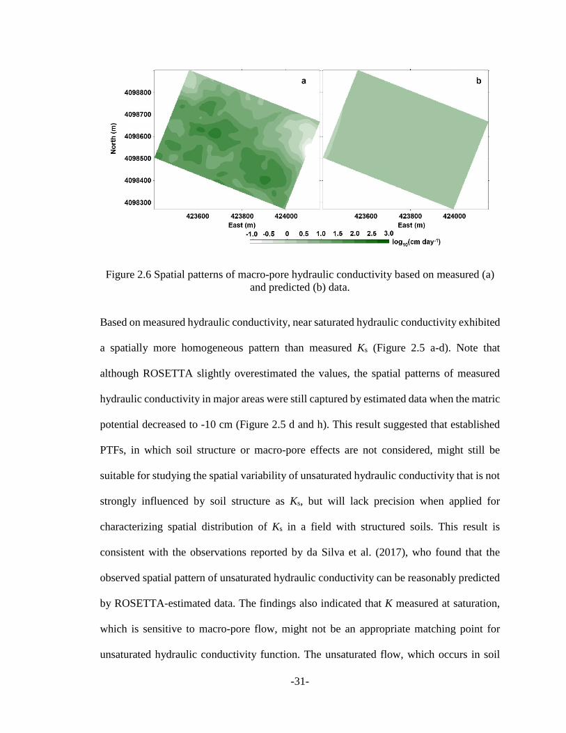
(e-h) data…………………………………………………………………..…30 Figure 2.6 Spatial patterns of macro-pore hydraulic conductivity based on measured (a)
and predicted (b) data. .................................................................................... 31 Figure 3.1 Soil water retention data of four soils with macro-pores in this study. ........... 46 Figure 3.2 Textural composition of soils investigated in this study. ................................ 48 Figure 3.3 Measured and estimated saturated hydraulic conductivity, Ks, for the seven PTF
models investigated.………… …………………………………………….....51 Figure 3.4 Estimated saturated hydraulic conductivity for the field samples on different
methods. ......................................................................................................... 52 Figure 3.5 Decrease in relative hydraulic conductivity as a function of soil water pressure
head. ................................................................................................................ 53 Figure 3.6 Distributions of model coefficients (clay and macro-porosity) and intercept
based on 100 times of simulation. ................................................................. 61 Figure 3.7 Distributions of root mean square error (RMSE), Nash-Sutcliffe efficiency (NSE)
and coefficient of determination (R2) based on 100 validation runs. .............. 61 Figure 3.8 Average regression coefficient of each variable (left) and training error (right)
related to number of realizations. .................................................................. 63 Figure 3.9 The performance of pedo-transfer functions based on 100 validation runs. ... 66 Figure 4.1 Sampling grid and array of data for state-space modeling. ............................. 72 Figure 4.2 Spatial distributions of soil hydraulic conductivity and physical properties across
the field. .......................................................................................................... 77 Figure 4.3 Autocorrelation functions (ACF) for soil hydraulic conductivity. .................. 79 Figure 4.4 Cross-correlation functions (CCF) for soil hydraulic conductivity and physical
properties. ...................................................................................................... 80 Figure 4.5 Bivariate state-space analysis of saturated hydraulic conductivity (Ks) and macro-
porosity (φ) using all Ks observations (a) and 50% of the Ks observations (b), respectively. ..................................................................................................... 81
Figure 4.6 Multivariate state-space analysis of near-saturated hydraulic conductivity (K-10), silt content, clay content, and macro-porosity (φ) using all K-10 observations (a) and 50% of the K-10 observations (b), respectively. ......................................... 83

ix
Figure 4.7 Multivariate state-space analysis of near-saturated hydraulic conductivity (K-10), silt content, and clay content using all K-10 observations (a) and 50% of the K-10 observations (b), respectively. ......................................................................... 84
Figure 4.8 Autoregressive prediction of saturated hydraulic conductivity (Ks), based on Ks and macro-porosity (φ). Autoregression coefficients were obtained from state-space analysis (Figure 4.5). ............................................................................. 85
Figure 4.9 Autoregressive prediction of near-saturated hydraulic conductivity (K-10), based on K-10, silt content, clay content, and macro-porosity (φ). Autoregression coefficients were obtained from state-space analysis (Figure 4.6). ................ 86
Figure 4.10 Autoregressive prediction of near-saturated hydraulic conductivity (K-10), based on K-10, silt content, and clay content. Autoregression coefficients were obtained from state-space analysis (Figure 4.7). ......................................... 87

-1-
Chapter 1 Introduction
Irrigation is vital to our food production and food security. Irrigated areas are expected to
rise in forthcoming years whereas fresh water will be increasingly diverted to meet the
increasing demand of domestic and industrial use (Evans and Sadler, 2008; Bianchi et al.,
2017). Society faces a critical challenge in the future: increasing agricultural production
using limited water resources and maintaining healthy ecosystems at local and global scales.
Kentucky is perceived as a “water-rich” state with a moderate humid subtropical climate
and abundant rainfall (average annual precipitation varies from 1060 mm in the north to
1502 mm in the southwest of the state) (Chattopadhyay and Edwards, 2016). However,
Kentucky can experience extended periods of dry weather ranging from single-season
events to multi-year events (e.g., disastrous droughts in 2007 and 2012) (Kentucky Energy
and Environment Cabinet, 2008). Western Kentucky is projected to see a moderate summer
drought in the following decades (Cook et al., 2015). Due to a limited water supply in many
parts of Kentucky, irrigation has always been limited (Murdock, 2000). Following the
drought in the year 2012, many farmers installed center pivot irrigation systems in their
fields. Although interest in irrigation is gaining momentum among Kentucky farmers, little
research has been conducted on water-efficient irrigation in Kentucky. The development
of effective field water resources management is crucial to conserve water during drought
mainly through avoiding over-irrigation and using limited water resources in the most
efficient way.
Conventional uniform irrigation management, which ignores the considerable inherent soil
spatial variability in physical and hydraulic properties, treats the field homogeneously in
-2-
terms of water application amount and intensity and might result in both excessive and
deficit water availability at some specific areas in the field, and lead to yield and nutrient
losses (King et al., 2006; Liang et al., 2016). One approach for optimizing field water
management is site-specific irrigation management, which aims at applying water in
accordance with the spatial heterogeneity of soil properties in the field. Such management
practice requires quantification of soil spatial variability across the field (Mzuku et al.,
2005; Sadler et al., 2005).
Infiltration variability across a field plays an important role in irrigation management and
in turn affects crop yields and farm economics (Jaynes and Clemmens, 1986; Wallender
and Rayej, 1987; Hoover and Jarrett, 1989; Jaynes and Hunsaker, 1989). Infiltration refers
to the soil’s ability to allow water moving into and through the soil profile. Due to
variations in soil hydraulic properties and topography as well as external factors such as
compaction and tillage practices, infiltration rate and resulting water movement vary
among locations within the field after one irrigation event (Evans and Sadler, 2008). Soil
hydraulic conductivity (K), especially saturated hydraulic conductivity (Ks), is a crucial
property governing soil water dynamics including infiltration and percolation (Huang et al.,
2016). Therefore, accurate knowledge of saturated hydraulic conductivity and its spatial
variability in an irrigated field is important for developing site-specific irrigation
management and provides essential parameters for water balance and solute transport
models (Bevington et al., 2016).
Using representative soil samples from the study area, saturated hydraulic conductivity is
measured with widely used techniques, such as borehole infiltrometer and Amoozemeter,
in the field, or with constant/falling head permeameter in the laboratory (Klute and Dirksen,

-3-
1986; Amoozegar, 1989; Stephens, 1992). However, Ks often exhibits high spatial
heterogeneity (Nielsen et al., 1973; Schaap and Leij, 1998b). Large numbers of soil
samples are generally required to derive the average Ks in a study area and even more
samples may be necessary to accurately characterize the spatial variability of Ks in that area.
For example, Vieira et al. (1981) characterized the spatial variability of infiltration rate
based on 1280 measurements. By comparing different scenarios, they found that at least
128 field-measured values were required in order to obtain useful spatial information in a
field with an area of 0.88 ha (Vieira et al., 1981). Since direct measurements of Ks are
labor-intensive and time-consuming, the evaluation of spatial heterogeneity of Ks based on
measured data is prohibitive for field or larger research scales. Therefore, predicting Ks
from more easily measured soil properties (e.g., soil texture, bulk density, organic matter,
or electrical conductivity) has become an active research area (Wang et al., 2012a; Rezaei
et al., 2016; Zhao et al., 2016). The functions that link soil hydraulic properties with more
readily available soil properties are defined as pedo-transfer functions (PTFs) (Bouma and
Lanen, 1987).
Pedo-transfer functions can be developed either from multiple regression methods (Cosby
et al., 1984; Puckett et al., 1985; Saxton et al., 1986; Vereecken et al., 1990; Merdun et al.,
2006), regression and classification trees (Lilly et al., 2008; Jorda et al., 2015), and artificial
neural network (Schaap et al., 2001; Zhao et al., 2016). In the past decades, PTFs have
been widely used as an alternative approach to estimate the spatial variability of hydraulic
conductivity at different research scales. In a combination of PTFs and geostatistical
methods, a Ks map of Spain was successfully constructed (Ferrer Julià et al., 2004). Pedo-
transfer functions were applied to studying the spatial variability of Ks across China (Dai

-4-
et al., 2013). In a recent research, ROSETTA PTF was used to characterize the Ks at global
scale (Montzka et al., 2017). However, the application of PTFs in estimating the spatial
variability of Ks at the field scale is rarely reported (Parasuraman et al., 2006). Pedo-
transfer functions were usually derived at a large scale using large datasets, and soil texture,
bulk density as well as organic matter were commonly used as input variables. The spatial
behavior of Ks and its influencing factors may change with increase or decrease in the
domain of investigation (Wang et al., 2013). At large scales (e.g., the domain of a continent
or a country), soil texture might be a dominant factor of the magnitude and spatial variation
of Ks. On the other hand, at the small scale of a farmer’s field, the spatial heterogeneity of
Ks due to soil texture variation can be masked by soil structure as well as landscape position,
topography-related hydrologic conditions and agricultural management (Zimmermann et
al., 2013). Therefore, a PTF that is valid for a large area is not necessarily able to model
small scale phenomena well (Vereecken et al., 2010). The application of PTFs to describe
the spatial variability of Ks at the field scale needs to be critically evaluated. Inclusion of
important soil structural information might be beneficial to developing PTFs for estimating
Ks at the field scale. However, mainly owing to soil structure is relatively difficult to
measure, little progress has been made in improving PTFs by incorporating quantitative
soil structural information.
In addition, current PTFs overlook the spatial covariance between soil properties and
assume that all the soil variables are spatially independent from each other. Therefore, these
PTFs often perform unsatisfactorily when field-scale estimations of hydraulic properties
are needed (Nielsen and Alemi, 1989; Yang and Wendroth, 2014). Most recently, a state-
space modeling approach, which considers the spatial dependencies between variables, was

-5-
used to develop models to estimate hydraulic properties, and has been demonstrated to be
a more effective tool for quantifying the relationships between hydraulic properties and
other soil variables compared with the equivalent linear regression equations and artificial
neural network models (Comegna et al., 2010; Zhao et al., 2017; Qiao et al., 2018a; Qiao
et al., 2018b). However, the application of state-space models in spatially estimating soil
hydraulic properties, such as Ks, has not been adequately studied (Yang et al., 2018).
Guided by the above information, this study aims at improving field water management
through characterization of the spatial variability of saturated hydraulic conductivity and
its influencing factors in a farmer’s field located in western Kentucky. The specific
objectives of this study were to (1) critically evaluate the performance of PTFs in
estimating the spatial variability of hydraulic conductivity at and near saturation in a
farmland, (2) quantify the contribution of structural macro-pores to saturated water flow in
the studied field, (3) examine if the estimation of Ks at the field scale with PTFs can be
improved by including quantitative soil structural information (such as macro-porosity),
and (4) make an attempt to quantify the spatial relationships between hydraulic
conductivity and other soil physical properties by state-space modeling approach.
In Chapter 2, the spatial pattern of hydraulic conductivity was created with co-
regionalization analysis and compared with the spatial variability of hydraulic conductivity
predicted with PTFs. Macro-pore hydraulic conductivity was calculated and used to
identify the structural macro-pore effects in this no-till agricultural land. The purpose of
this study was to answer the question whether the spatial pattern of hydraulic conductivity
in structural soil can be reasonably captured by existing PTFs. According to Chapter 2, soil
structural information is important for predicting Ks. In Chapter 3, soil macro-porosity was

-6-
calculated from soil water retention curve and used as a structural parameter in developing
a new PTF. The performance of new PTF in estimating Ks at the field scale was then
evaluated by comparing with established PTFs, in which soil structural information was
excluded. In Chapter 4, a pioneering research approach using autoregressive state-space
analysis to estimate the spatial variation of hydraulic conductivity across a field was
conducted. This chapter tried to characterize the spatial correlations of hydraulic
conductivity with the soil physical properties, and evaluate if the spatial pattern of
hydraulic conductivity can be better described by state-space modeling compared with
current PTFs that ignore the spatial dependence between soil variables. Results from
studies presented in this dissertation provide a basis for modeling water/solute transport in
the vadose zone, and site-specific resources management.
Copyright © Xi Zhang 2019

-7-
Chapter 2 Assessing field-scale variability of soil hydraulic conductivity at and near saturation
2.1 Introduction
Hydraulic conductivity at and near saturation of the soil surface layer plays an important
role in partitioning precipitation or irrigation water into surface runoff and soil water, and
regulating water transport in the vadose zone (Børgesen et al., 2006; Jarvis et al., 2013;
Dingman, 2015; Ugarte Nano et al., 2015; Gadi et al., 2017). Soil saturated hydraulic
conductivity (Ks), which determines the maximum capacity of soil to transmit water, is a
crucial hydraulic parameter for hydrological models (e.g., HYDRUS, RZWQM2)
(Mallants et al., 1997; Zhao et al., 2016). In many field soils, Ks is strongly influenced by
soil structure and macro-pores, and exhibits high spatial heterogeneity (Jarvis et al., 2002;
Strudley et al., 2008). Due to the high spatial variability of Ks, the optimum application
rate and amount of irrigation water differs between specific areas within the same field (Al-
Karadsheh et al., 2002). Accurate characterization of the spatial variation of Ks at the field
scale is therefore important for precision irrigation management and identification of local
management zones (Gumiere et al., 2014). A map of the spatial distribution of Ks can
become useful for guiding site-specific irrigation, helping farmers apply the right amount
of water in the right areas at the right intensity and time while minimizing the potentially
environmental risks, e.g., leaching, surface runoff, oxygen deficiency through over-
irrigation, and plant-water stress and yield loss through under-irrigation.
Saturated hydraulic conductivity can be measured either in the field with in-situ methods
(e.g., borehole infiltrometer, Amoozemeter) or in the laboratory with a permeameter (Klute
and Dirksen, 1986; Amoozegar, 1989; Stephens, 1992). However, Ks is a parameter that
-8-
exhibits enormous spatial variability (Nielsen et al., 1973; Schaap and Leij, 1998b). Large
numbers of soil samples are generally required to accurately characterize Ks in a study area
(Yao et al., 2015). Accurate characterization of Ks using direct measurements, therefor, are
arduous, time-consuming, and expensive (Li et al., 2007; Wang et al., 2012a). To overcome
these limitations and to characterize the spatial variability of Ks for large regions, alternative
approaches have been developed to estimate Ks indirectly through more easily measurable
soil properties that may already exist from soil surveys or from existing soil databases.
Among these alternative approaches, pedo-transfer functions (PTFs) have been developed
and are increasingly being used to estimate Ks (Wösten et al., 2001; Pachepsky et al., 2006;
McBratney et al., 2011). In the past decades, the accuracy and reliability of PTFs for
estimating Ks have been critically evaluated (Tietje and Hennings, 1996; Schaap and Leij,
1998a; Wagner et al., 2001; Alvarez-Acosta et al., 2012; Yao et al., 2015). The PTF
estimate at a single point is usually compared with the measured value at the same location.
Although estimation of Ks at a single point is necessary for modeling water flow and solute
transport in a soil profile, a detailed description of the spatial variability or distribution of
Ks is needed for field water management with distributed hydrological models (Liao et al.,
2011). Several authors have studied the spatial characterization of unsaturated hydraulic
conductivity (soil water pressure, h, less than -10 cm) by using both measured data and
PTF predictions (e.g., Romano, 2004; da Silva et al., 2017), however, far fewer studies
investigated the performance of PTFs in describing spatial structure or characterizing
spatial pattern of Ks in a field and the results are inconsistent (Springer and Cundy, 1987;
Leij et al., 2004). For unsaturated hydraulic conductivity, although PTF estimates revealed
stronger spatial dependence than measured data and the generated spatial pattern of

-9-
hydraulic conductivity depended on the choice of PTFs, kriged maps of hydraulic
conductivity based on measurements and on PTF estimates showed similarities in their
spatial variations. (Romano, 2004; da Silva et al., 2017).
Unsaturated water flow at h ≤ -10 cm mainly occurs in the soil matrix, and soil texture
places a significant impact on unsaturated hydraulic conductivity (Lin et al., 1999b; Schaap
and Leij, 2000). For saturated water flow (h = 0 cm), the behavior differs. Hydraulic
conductivity at saturation is sensitive to even small volumes of macro-pores, which are
affected by agricultural management and biological activities (Rienzner and Gandolfi,
2014). In field soils with structural macro-pores, a large decrease (e.g., several orders of
magnitude) in hydraulic conductivity is often observed as water pressure head even slightly
drops from saturation to near saturated conditions (-10 cm < h < 0 cm) (Jarvis and Messing,
1995; Jarvis et al., 2002; Braud et al., 2017). Near saturated hydraulic conductivity is
therefore used to identify macro-pore effects in a field. The influence of basic soil physical
properties (e.g., texture, bulk density, and organic matter content), which are common PTF
predictors, on Ks is usually masked by macro-pore effects (Buttle and House, 1997).
However, soil structure or macro-pore information is not included in most published PTFs
(Lin et al., 1999b; Weynants et al., 2009; Vereecken et al., 2010). Models that relate Ks to
basic soil physical properties alone may therefore not accurately predict Ks for soils with
pronounced structure (Lin et al., 1999a). Since PTF predictors (i.e. basic soil physical
properties) can be only sampled for a limited number of points in an area, PTF estimates
at these points have to be combined with spatial interpolation to make predictions at
unsampled locations with the result that the estimated spatial variability less reflects the
behavior of the target variable than that of the PTF input variables. At each sampled

-10-
location, the uncertainty (e.g., measurement errors) in the input variables also causes
uncertainty in the PTF estimates. This uncertainty is further propagated to the interpolated
points and it is larger the farther away an interpolated point is located from the next
measured point (Chirico et al., 2007). Moreover, the spatial interpolation of PTF-predicted
data is dominated by the spatial variability pattern of the underlying predictors, which may
deviate from the spatial variability pattern of measured hydraulic conductivity data,
especially if soil structural features affect their magnitude, such as macro-pores. Springer
and Cundy (1987) compared measurements of Ks with the predicted data obtained from
two published PTFs at the field scale, and the semivariogram of the measured data was
well reproduced by one of the PTFs. They also found that the correlation length was short
for the field-measured data. Leij et al. (2004) did similar work in a field with structural soil,
however, their findings were discouraging. All the selected PTFs failed to capture the
spatial structure of observed Ks. Furthermore, Pringle et al. (2007) emphasized that PTFs
are scale-dependent. PTF-estimated data is unable to provide a reasonable portrayal of the
spatial variations exhibited by measured data at all spatial scales (Pringle et al., 2007).
These studies indicate that there are still significant uncertainties about whether the spatial
variability of Ks observed in a field can be captured by PTF predicted data. Therefore,
characterizing the field-scale spatial pattern of Ks predicted with a PTF still needs to be
critically evaluated. To this end, the primary objective of this study was to characterize the
spatial variability of hydraulic conductivity at and near saturation in an agricultural field
by geostatistical analysis using both measured and PTF estimated data.

-11-
2.2 Materials and Methods
2.2.1 Site description and soil sampling
This research was conducted in a farmland (~30 ha) located in Caldwell County, Kentucky,
United States (37°1′42″-37°1′58″N, 87°51′11″-87°51′33″W) (Figure 2.1). At this area, the
mean annual precipitation is 1300 mm with a mean annual temperature of 15 °C (US
Climate Data, 2016). Wheat/ double-crop soybean/ corn rotation is practiced in this field.
Undisturbed soil cores were sampled in a 71 m by 71 m grid of 48 locations from 7-13 cm
depth by using cutting rings (diameter: 8.4 cm, height: 6 cm, volume: 332 cm3). Bulk soil
samples were also collected from each point. Soil cores were used to measure saturated
and near-saturated hydraulic conductivity, and bulk density. Disturbed soil samples were
air-dried and passed through a 2-mm sieve for other soil physical property analyses.
2.2.2 Laboratory analysis
Soil texture was determined by the sieving and the pipette method (Gee and Or, 2002).
According to USDA textural classification, three textural classes (silt, silty loam and silty
clay loam) were observed in the field (Figure 2.2). Silty loam was the predominant soil
texture. The core method was used to measure bulk density (ρb) (Grossman and Reinsch,
2002). The bulk density ranged from 1.33 to 1.77 g cm-3 (Table 2.1). Soil organic matter
(SOM) was measured with the combustion method (Nelson and Sommers, 1982). The range
of SOM was between 0.70 and 2.38% (Table 2.1).

-12-
Figure 2.1 Study area and sampling locations.

-13-
Table 2.1 Descriptive statistics for observed and Rosetta estimated hydraulic conductivity, and basic soil physical properties over the field (N= 48).
Variables † Maximum Minimum Mean S.D. ‡ K-S ‡ Observed data
Ks, cm day-1 16307 0.02 31* 2815 0.40 K-1, cm day-1 217 0.07 3.80* 37 0.33 K-5, cm day-1 26 0.06 1.40* 4.97 0.30 K-10, cm day-1 5.66 0.04 0.79* 1.09 0.19
Ks, log10 (cm day-1) 4.21 -1.80 1.49 1.36 0.08 K-1, log10 (cm day-1) 2.34 -1.15 0.58 0.74 0.14 K-5, log10 (cm day-1) 1.42 -1.22 0.15 0.54 0.07 K-10, log10 (cm day-1) 0.75 -1.40 -0.10 0.44 0.11
Sand, % 11 2 4 1 0.14 Silt, % 85 57 79 6 0.15 Clay, % 33 10 17 5 0.18 ρb, g cm-3 1.77 1.33 1.61 0.07 0.10
ECa, mS m-1 8.40 2.80 4.64 1.23 0.09 SOM, % 2.38 0.70 1.38 0.31 0.09
ROSETTA estimated data Ks, log10 (cm day-1) 1.49 0.37 0.87 0.22 0.12 K-1, log10 (cm day-1) 1.46 0.26 0.82 0.24 0.11 K-5, log10 (cm day-1) 1.40 0.13 0.73 0.25 0.12 K-10, log10 (cm day-1) 1.35 0.02 0.65 0.26 0.12
† Ks, saturated hydraulic conductivity; K-1 K-5 and K-10, hydraulic conductivity at potentials of -1 cm, -5 cm and -10 cm; ρb, bulk density; ECa, apparent electrical conductivity; SOM, soil organic matter.
‡ S.D., standard deviation; K-S, Kolmogorov–Smirnov test for normality (for α=5%, critical value is 0.196).
* Geometric mean.

-14-
Figure 2.2 Textural composition of soils investigated in this study.
Saturated hydraulic conductivity (Ks) was determined using a laboratory permeameter
(Eijkelkamp, Netherlands) based on Darcy’s law under either constant or falling head
conditions depending on the individual percolation rate of each sample (Klute and Dirksen,
1986). Near-saturated hydraulic conductivity is useful in studying the influence of soil
structural macro-pores on hydraulic conductivity and rapid infiltration (Jarvis et al., 2013).
Hydraulic conductivity at potentials of -1 cm (K-1), -5 cm (K-5) and -10 cm (K-10) were
therefore measured with a self-developed double pressure plate-membrane apparatus with
two tension plates at the upper and lower ends of the soil core, which are similar to those
used with tension infiltrometer (Wendroth and Simunek, 1999). The computation of K(h)
is based on Buckingham-Darcy’s law. The ranges of Ks, K-1, K-5, and K-10 were between 0.02
and 16307, 0.07 and 217, 0.06 and 26, and 0.04 and 5.66 cm day-1, respectively. Hydraulic
conductivity data (cm day-1) was further log-transformed (Table 2.1). The ranges of log10 Ks,

-15-
log10 K-1, log10 K-5, and log10 K-10 were between -1.80 and 4.21, -1.15 and 2.34, -1.22 and
1.42, and -1.40 and 0.75, respectively. For several soil samples with low Ks, the near-
saturated hydraulic conductivity was slightly higher than Ks. Those slight inconsistencies
in the data might be introduced by different measurement methods (Vereecken et al., 2010).
The relatively low conductivity of some samples changed little regardless whether the
sample was measured under saturated or slightly unsaturated conditions since these
samples remain fully saturated due to capillary forces even under slightly negative pressure,
and our measurement results obtained with different methods just reflected measurement
uncertainty. For soil samples with low permeability, the falling head method was used to
measure Ks. During this process, evaporation cannot be completely avoided. This might
also cause underestimation in Ks.
2.2.3 Estimates with pedo-transfer functions
Over the past three decades, a large number of PTFs have been developed to estimate
hydraulic conductivity. Soil texture, bulk density and organic matter were widely used as
input data in these established PTFs (Wösten et al., 2001). Among these published PTFs,
ROSETTA (derived from North American and European soils) and HYPRES (derived
from European soils) are the most widely used PTFs (Wösten et al., 1999; Schaap et al.,
2001; McBratney et al., 2011). ROSETTA was developed based on artificial neural
network analysis and includes five hierarchical models (H1 - H5) (see Schaap et al., 2001
for detail). The hierarchical structure in ROSETTA provides users with flexibility towards
available input data. ROSETTA is able to estimate Ks as well as unsaturated hydraulic
conductivity function parameters for the Mualem-van Genuchten model. A user-friendly
computer program was developed to make the estimation with ROSETTA even more

-16-
convenient. Therefore, ROSETTA was selected as an example to investigate whether PTFs
reliably describe the spatial variability of hydraulic conductivity observed in a field. Based
on available measured soil physical properties, the H3 model (sand, silt, clay, and bulk
density) was used to predict hydraulic conductivity in this study. Note that an external PTF
might lose its validity if it is used for soils that fall outside the textural range of data
originally used to derive the PTF. The estimation of hydraulic properties based on PTFs
should be restricted to soils that fall within the range of soil textures that were used to
develop the PTFs (Wösten, 1997). In this study, local soil properties are within the range
of the dataset that was used to derive ROSETTA.
Saturated hydraulic conductivity was indirectly estimated from ROSETTA. Mualem-van
Genuchten model parameters were predicted by ROSETTA and near saturated hydraulic
conductivity (h = -1, -5, -10 cm) was calculated by Eq. 2.1 (van Genuchten, 1980):
𝐾𝐾(ℎ) = 𝐾𝐾s�1−|𝛼𝛼ℎ|𝑛𝑛−1[1+|𝛼𝛼ℎ|𝑛𝑛]−𝑚𝑚�2
[1+|𝛼𝛼ℎ|𝑛𝑛]𝑚𝑚/2 (2.1)
where Ks (cm day-1) is the ROSETTA-estimated saturated hydraulic conductivity, h (cm) is
soil water pressure, α (cm-1) is related to the inverse of the air-entry pressure head, m (-) and
n (-) are empirical shape parameter (m=1- 1/n). α and n were also predicted by ROSETTA.
ROSETTA estimated hydraulic conductivity data (cm day-1) was also log-transformed
(Table 2.1). The ranges of log10 Ks, log10 K-1, log10 K-5, and log10 K-10 were between 0.37
and 1.49, 0.26 and 1.46, 0.13 and 1.40, and 0.02 and 1.35, respectively.
-17-
2.2.4 Geostatistical analysis
Hydraulic properties in field soils are highly variable, and any individual measurement can
only provide information about the immediate vicinity of the sampled location. Information
about hydraulic properties at places where no measurements are taken has to be inferred
from the known values at the sampled points since only a limited number of measurements
can be taken in an area (Nielsen et al., 1973; Jury and Horton, 2004). Various strategies
(e.g., inverse distance weighting, kriging, cokriging) can be used to interpolate spatial data
(Webster and Oliver, 2007). Geostatistics (e.g., kriging and cokriging) is generally
considered as the best method for spatial interpolation and has been successfully used in
studying the spatial variation of soil hydraulic properties (Vieira et al., 1981; Vauclin et al.,
1983; Goovaerts, 1999; Ferrer Julià et al., 2004; Romano, 2004; Iqbal et al., 2005; Wang
et al., 2013; Fu et al., 2015). Kriging is a linear interpolation that utilizes a semivariogram
to estimate a variable at an unsampled location using weighted neighboring measured
values (Nielsen and Wendroth, 2003). The performance of kriging in interpolating spatial
data greatly depends on the quantity and quality of the measurements and their spatial
continuity (Miller et al., 2007) as well as their behavior in the scale-triplet (Blöschl and
Sivapalan, 1995). However, only limited Ks data are available since the cost and labor of
intensively measuring Ks in a field is prohibitive (Alemi et al., 1988). In a field with high
spatial variability of Ks, it can be a challenge to create a set of measured Ks at a resolution
that reveals a satisfactory variability structure to support kriged estimates of Ks at
unsampled locations with acceptable accuracy. When Ks is undersampled and the identified
variability structure is weak, kriging is not well supported, and the uncertainty of estimation
poses a challenge as well (Ersahin, 2003). Alternatively, cokriging utilizes spatial

-18-
information of two or more variables (one is the primary variable, the other is the ancillary
variable) along with spatial cross-correlation between the two variables to estimate the
undersampled variable (i.e., primary variable) at unobserved locations. The ancillary
variable is spatially correlated with the variable of interest, and can be easily measured and
densely sampled (Alemi et al., 1988; Nielsen and Wendroth, 2003). By using clay content
(Alemi et al., 1988), bulk density (Ersahin, 2003) or water-stable aggregates (Basaran et
al., 2011) as ancillary variable, cokriging has been proven to be superior to kriging in
characterizing the spatial variability of Ks when Ks is only sparsely sampled in an area.
Although apparent electrical conductivity has not been used as an ancillary variable in
cokriging to estimate Ks, investigating the spatial association of Ks to apparent electrical
conductivity might be another promising way to estimate the spatial distribution of Ks
across a field. Apparent electrical conductivity (ECa) is a simple, efficient and inexpensive
measurement, and can be densely measured over large areas (Sudduth et al., 2005). Similar
to water flow in soil, apparent electrical conduction (mainly through electrolyte in
sufficiently moist soil) occurs in the same network of pores and channels (Corwin and
Lesch, 2003; Doussan and Ruy, 2009). ECa is influenced by a variety of soil properties
including soil clay content, porosity, pore connectivity, moisture, salinity, and organic
matter (Corwin and Lesch, 2005; Doussan and Ruy, 2009; Chaplot et al., 2010). These
factors influencing ECa also have effects on soil hydraulic conductivity. In recent studies,
ECa was successfully used as a predictor in linear regression PTFs to calculate Ks (Chaplot
et al., 2011; Rezaei et al., 2016). Therefore, ECa can be considered as an ancillary variable
and was used in cokriging to facilitate the estimation of Ks in this research.

-19-
Soil apparent electrical conductivity (ECa) at shallow depth (0-30 cm) was densely
measured in the field (Figure 2.1) (the distance between two neighboring transects was
about 17 m and the distance between two neighboring points along each transect was
approximately 2 m) using a Veris 3150 (Reyes et al., 2018). Apparent electrical
conductivity and hydraulic conductivity were not measured at exactly the same coordinates.
In order to perform classic cross semivariogram, the values of ECa points (3~5 points)
located within a radius of 2 m around each hydraulic conductivity sampling location were
averaged and this average value was used as ECa value in the point of hydraulic
conductivity. ECa values at the points of hydraulic conductivity ranged from 2.80 to 8.40
mS m-1 with a mean of 4.64 mS m-1 (Table 2.1).
Geostatistical analysis was then conducted to characterize the spatial pattern of hydraulic
conductivity and to assess the capability of ROSETTA in describing the spatial variability
of hydraulic conductivity in the field. Prior to geostatistical analysis, Kolmogorov-Smirnov
(K-S) test (at the 5% significance level) was used to evaluate the normality of each data
distribution (Bitencourt et al., 2016). The K-S test quantifies the maximum difference
between the observed distribution function of the sample and the theoretical distribution
function (Massey, 1951). All the data passed the K-S test, since the calculated maximum
differences were below the critical value at the 5% significance level (Table 2.1). The result
indicated that log-transformed measured hydraulic conductivity, ROSETTA estimated
hydraulic conductivity, and basic soil physical properties tended to follow the normal
distribution. Note that ECa data (N = 48) at the locations of hydraulic conductivity was a
subset of all ECa measurements (N= 7416) in the study field. Apparent electrical
conductivity data including all the points failed the K-S test as a result of the huge number

-20-
of samples considerably reducing the critical value (for α= 5%, critical value is 1.36/√𝑁𝑁).
Since ECa data (N = 48) had the same number of observations as hydraulic conductivity
data and was normally distributed, ECa data (N= 7416) distribution can still be considered
as a normal distribution (Reyes et al., 2018).
Experimental semivariograms and cross semivariograms were calculated to describe the
spatial variance structure and identify the input parameters for cokriging spatial
interpolation (Nielsen and Wendroth, 2003). The semivariogram and cross semivariogram
were computed by Eq. 2.2 and Eq. 2.3, respectively.
𝛾𝛾(ℎ) = 12𝑁𝑁(ℎ)
∑ [𝑍𝑍𝑖𝑖(𝑥𝑥𝑖𝑖) − 𝑍𝑍𝑖𝑖(𝑥𝑥𝑖𝑖 + ℎ)]2𝑁𝑁(ℎ)𝑖𝑖=1 (2.2)
𝛤𝛤(ℎ) = 12𝑁𝑁(ℎ)
∑ [𝐴𝐴𝑖𝑖(𝑥𝑥𝑖𝑖) − 𝐴𝐴𝑖𝑖(𝑥𝑥𝑖𝑖 + ℎ)][𝐵𝐵𝑖𝑖(𝑥𝑥𝑖𝑖) − 𝐵𝐵𝑖𝑖(𝑥𝑥𝑖𝑖 + ℎ)]𝑁𝑁(ℎ)𝑖𝑖=1 (2.3)
where h is the separation distance or lag distance, N(h) is the number of data pairs for the
separation distance h, Zi(xi) is a measured variable at spatial location xi, Zi(xi + h) is a
measured variable at spatial location xi + h, Ai and Bi indicate the primary and the ancillary
variables, respectively. The shape of semivariogram depends upon the nature of the spatial
variability, number and spacing of the observations, and lag class interval length. In order
to obtain a semivariogram revealing obvious spatial structure, different lag class interval
lengths were used in the calculation. The lag class interval length was 50 m for Ks and K-10,
while the lag class interval length was 40 m for K-1 and K-5.
Experimental semivariograms and cross semivariograms were fitted to an empirical model
including an exponential component and a Gaussian component (Eq. 2.4) (Oliver and
Webster, 2014) on top of the nugget contribution to variance.

-21-
𝛾𝛾(ℎ) = 𝐶𝐶0 + 𝐶𝐶1 �1 − exp �− ℎ𝑎𝑎1�� + 𝐶𝐶2 �1 − exp �− ℎ2
𝑎𝑎22�� (2.4)
where C0 represents the nugget effect; C1 and C2 are the partial sills of exponential and
Gaussian components, respectively, and sill (total variation) equals to C0+C1+C2; a1 and a2
are the ranges of exponential and Gaussian components, respectively; h is the lag distance.
The two model functions were selected and determined principally on sum of square
residuals (SSR), coefficient of determination (r2) as well as visual fit (Cambardella et al.,
1994; Wang et al., 2013).
The spatial distribution maps of hydraulic conductivity were generated using fitted
semivariogram and cross semivariogram parameters through cokriging, which estimated
the values of hydraulic conductivity at unobserved locations by utilizing Eq. 2.5.
𝐴𝐴∗(𝑥𝑥0) = ∑ 𝜆𝜆𝐴𝐴𝑖𝑖𝐴𝐴𝑖𝑖(𝑥𝑥𝑖𝑖) + ∑ 𝜆𝜆𝐵𝐵𝐵𝐵𝐵𝐵𝐵𝐵(𝑥𝑥𝐵𝐵)𝑞𝑞𝐵𝐵=1
𝑝𝑝𝑖𝑖=1 (2.5)
where A*(x0) is the value of primary variable to be estimated at the location of x0, Ai(xi) is the
known value of primary variable at the sampling site xi, Bj(xj) is the known value of ancillary
variable at the sampling site xj, λAi and λBj are weights (∑ 𝜆𝜆𝐴𝐴𝑖𝑖 = 1𝑝𝑝𝑖𝑖=1 , ∑ 𝜆𝜆𝐵𝐵𝐵𝐵 = 0𝑞𝑞
𝐵𝐵=1 ), p and
q are the number of observed sites around x0 that are within the zone of correlation.
All the data analyses and visualization were accomplished by libraries (Gstat and Nortest)
included in the R statistics environment, ArcGIS 10.4.1, and Microsoft Office Excel 2016.

-22-
2.3 Results and Discussion
2.3.1 Spatial structure of hydraulic conductivity
Semivariograms and cross semivariograms based on measured and ROSETTA estimated
data are shown in Figure 2.3 and 2.4. A nested model including an exponential and a
Gaussian component was used to fit the experimental semivariograms and cross
semivariograms. Theoretically, semivariogram increases with distance between sample
locations to a plateau or constant value (total semivariance) that is found for a given
separation distance (the range of spatial dependence) (Trangmar et al., 1986). Samples
separated by distances less than the range are spatially correlated, while those separated by
distances beyond the range are not spatially correlated (Wang et al., 2013). The range
indicates the maximum distance over which neighboring observations are spatially related.
Beyond the range, lag distances should be disregarded for interpolation (Nielsen and
Wendroth, 2003). The shorter the range, the more heterogeneous the variable; while the
longer the range, the more homogeneous or spatially continuous the variable behaves
(Marín-Castro et al., 2016). The non-zero semivariance at lag distance of zero is called
nugget semivariance (C0), which represents measurement errors or microvariability of the
variable occurring over smaller distance than the sampling interval (Trangmar et al., 1986;
Nielsen and Wendroth, 2003). The ratio between nugget and total semivariance (or relative
nugget effect, RNE) was used to evaluate the strength of spatial dependence: strong if the
ratio was less than 25%, moderate if the ratio was between 25% and 75%, and weak if the
ratio was greater than 75% (Cambardella et al., 1994).
The measured Ks was weakly spatially dependent (RNE= 81%), while measured near
saturated hydraulic conductivity was moderately spatially dependent with the relative

-23-
nugget effect ranging from about 46% to 48% (Figure 2.3 a-d). Saturated hydraulic
conductivity revealed a high relative nugget effect, which means Ks might exhibit strong
spatial dependence at a scale smaller than the sampling interval. Short range effect or
microheterogeneity of Ks was predominant in the field and could not be detected at the
scale of sampling (Trangmar et al., 1986). In Figure 2.3, note that the range values for near
saturated hydraulic conductivity were significantly larger than the range for Ks. This result
indicated that the spatial distribution of Ks was more heterogeneous than the spatial
distribution of near saturated hydraulic conductivity. The high heterogeneity of Ks might
be caused by macro-pore effects. At saturation, all pores conduct water and macro-pores
greatly contribute to water flow. The presence of one single macro-pore is barely
manifested in the total porosity, however, can greatly contribute to Ks if the pore is
continuous and even more if it is connected to other pores. As the water potential decreases,
the water-transmitting pores are those with smaller diameters (meso- and micro-pores).
Since macro-pores are mainly created by biological activity, their variation would be larger
than that of smaller pores inherent in the soil matrix (Mohanty et al., 1994). Saturated
hydraulic conductivity is highly sensitive to macro-pores. The inherent relationship
between Ks and macro-pores is therefore critical for the spatial structure of Ks at the field
scale (Marín-Castro et al., 2016).

-24-
Figure 2.3 Semivariograms for measured hydraulic conductivity and apparent electrical conductivity.
(a-d: semivariograms of measured hydraulic conductivity, e-h: semivariograms of apparent electrical conductivity, i-l: cross semivariograms of measured hydraulic
conductivity and apparent electrical conductivity)

-25-
For the ROSETTA-estimated hydraulic conductivity under saturated and near saturated
conditions, the corresponding relative nugget effect ranged from 28% to 32% (Figure 2.4).
Therefore, ROSETTA-estimated hydraulic conductivity showed a moderate spatial
dependence that is more pronounced than that of the measured hydraulic conductivity,
especially for Ks. Semivariances for hydraulic conductivity predicted by ROSETTA were
consistently smaller than those for measured hydraulic conductivity. Also, the range values
for ROSETTA-predicted data were larger than those for measured data. These results
indicated that ROSETTA-estimated hydraulic conductivity was more homogeneous or
continuous than measured data in the field. This phenomenon might be a result of the
estimates being calculated mainly based on soil texture-related properties. The spatial
structure of ROSETTA-estimated hydraulic conductivity followed the spatial structure of
clay content in the same field (Reyes et al., 2018). The spatial variability exhibited by
ROSETTA-estimates was therefore dominated by textural properties, which represented
the intrinsic variation (e.g., texture, mineralogy) inherited from soil genesis. However, in
many field soils, wet-range hydraulic conductivity is rather sensitive to soil structure,
which is strongly influenced by extrinsic variations (e.g., biological activity, agricultural
management) (Jarvis et al., 2002). Therefore, both intrinsic and extrinsic factors dominated
the semivariograms based on measurements, whereas only intrinsic factors influenced the
semivariograms of PTF estimates and the resulting interpolated maps. Compared with
intrinsic factors, extrinsic factors show much more spatial heterogeneity (Cambardella et
al., 1994; Romano, 2004). Therefore, measured hydraulic conductivity exhibited more
heterogeneity and weaker spatial dependence than ROSETTA estimates.

-26-
Figure 2.4 Semivariograms for estimated hydraulic conductivity with ROSETTA
Based on measured data, there was a good spatial correlation (RNE ranged from about 8%
to 42%) between hydraulic conductivity and apparent electrical conductivity (Figure 2.3 i-
l). This spatial relationship was represented by a rapidly decreasing cross semivariance
calculated between hydraulic conductivity and ECa values, which indicated that high values
of hydraulic conductivity corresponded to low values of ECa, and vice versa. This result
suggested that ECa could be used as an ancillary variable to predict the spatial distribution
of saturated and near saturated hydraulic conductivity with co-regionalization analysis in
the field. This approach would be preferred, as ECa is easily and accurately determined.
-27-
2.3.2 Spatial distribution of hydraulic conductivity
The fitted semivariogram and cross semivariogram models for measured hydraulic
conductivity were used in cokriging to generate hydraulic conductivity maps with a
resolution of 2 × 2 m2. Based on measured data, Ks showed very strong spatial variability
and was markedly different from the spatial patterns of near saturated hydraulic
conductivity (Figure 2.5 a-d). As soil water pressure approached zero, hydraulic
conductivity may depend to a large extent on small numbers of large pores (Bodhinayake
and Si, 2004). Soil pores with equivalent diameter larger than 300 μm (i.e., soil water
pressure of -10 cm) have profound influence on water movement in a field with well-
structured soils (Jarvis et al., 2002; Jarvis, 2007). Hydraulic conductivity at or close to
saturation (h ≥ -10 cm) is therefore important to illustrate the effects of soil macro-pores.
A significant drop in hydraulic conductivity near saturation is always observed in soils with
macro-pores when these pores drain under slight pressure decrease and do not participate
in flow anymore (Bouma, 1981; Jarvis et al., 2002; Børgesen et al., 2006). The difference
between Ks and K-10, i.e., Ks - K-10, is considered as macro-pore hydraulic conductivity
(Jarvis et al., 2013). By comparing measured hydraulic conductivity maps, a large reduction
(~95%) in hydraulic conductivity was observed in the field when soil water pressure
dropped from 0 to -10 cm. The drop in hydraulic conductivity was caused by emptying of
macro-pores. The spatial pattern of macro-pore hydraulic conductivity (Ks - K-10) in the field
was further characterized and is shown in Figure 2.6. The macro-pore hydraulic
conductivity calculated from measured data also exhibited high heterogeneity in the field
(Figure 2.6 a). Note that the Ks map and macro-pore hydraulic conductivity map generated
from measured data showed similarity for major areas in the field. This result indicated that

-28-
the macro-pore effect was predominant in the studied field and had a great contribution to
Ks. The presence of large pores increased the spatial variability of Ks in the field.
The spatial patterns of hydraulic conductivity in the same field were also generated with
ROSETTA-predicted data (Figure 2.5 e-h). The ROSETTA-estimated Ks map behaved
similar to the corresponding spatial distributions of estimated near saturated hydraulic
conductivity. Compared with measured data, the Ks map obtained using PTF-estimated
data showed less heterogeneity. Also, the macro-pore hydraulic conductivity calculated
based on PTF estimates was more homogeneous than the macro-pore hydraulic
conductivity calculated based on measured data in the field and had relatively small
magnitude (Figure 2.6 b). Actually, the predicted macro-pore hydraulic conductivity varied
by less than half-order of magnitude. This result indicated that ROSETTA is incapable of
identifying the macro-pore effects observed in the field. PTFs developed from large
databases like ROSETTA, by their nature, tend to smooth the spatial behavior of data. In
the field investigated, soil texture related properties reveal a relatively narrow range, much
narrower than the range represented in databases that were used for developing ROSETTA.
The influence of soil texture on hydraulic conductivity was masked by local processes,
such as soil structure. The variance of Ks observed in this field was therefore significantly
underestimated by ROSETTA, which is a texture-dominated PTF. Soil structural
information is particularly important in the wet range of the hydraulic conductivity function
(Weynants et al., 2009). Although soil structure is manifested to some degree in particle-
size distribution, it cannot be predicted solely from textural properties (Reynolds and
Zebchuk, 1996; Lin et al., 1999a; Ghafoor et al., 2013). Even if dry bulk density as a soil
structural parameter is included in the ROSETTA estimation, it is hardly correlated with

-29-
hydraulic conductivity at saturation because a few continuous macro-pores are hardly
causing a measurable difference in bulk density or total porosity but have a huge influence
on wet range hydraulic conductivity. However, soil structure or macro-pore information is
rarely incorporated in established PTFs, since it is difficult to quantify and unavailable in
most databases. Therefore, these models that relate soil Ks to textural properties and bulk
density alone cannot correctly predict Ks for soils with a pronounced structure and with a
hierarchical pore organization such as aggregated soils, e.g., many soils under no-till.

-30-
Figure 2.5 Spatial patterns of hydraulic conductivity based on measured (a-d) and
predicted (e-h) data.
-31-
Figure 2.6 Spatial patterns of macro-pore hydraulic conductivity based on measured (a) and predicted (b) data.
Based on measured hydraulic conductivity, near saturated hydraulic conductivity exhibited
a spatially more homogeneous pattern than measured Ks (Figure 2.5 a-d). Note that
although ROSETTA slightly overestimated the values, the spatial patterns of measured
hydraulic conductivity in major areas were still captured by estimated data when the matric
potential decreased to -10 cm (Figure 2.5 d and h). This result suggested that established
PTFs, in which soil structure or macro-pore effects are not considered, might still be
suitable for studying the spatial variability of unsaturated hydraulic conductivity that is not
strongly influenced by soil structure as Ks, but will lack precision when applied for
characterizing spatial distribution of Ks in a field with structured soils. This result is
consistent with the observations reported by da Silva et al. (2017), who found that the
observed spatial pattern of unsaturated hydraulic conductivity can be reasonably predicted
by ROSETTA-estimated data. The findings also indicated that K measured at saturation,
which is sensitive to macro-pore flow, might not be an appropriate matching point for
unsaturated hydraulic conductivity function. The unsaturated flow, which occurs in soil
-32-
matrix, might be overestimated by using measured Ks as matching point for hydraulic
conductivity function. Hydraulic conductivity measured at slightly unsaturated condition
or PTFs-estimated Ks might be a better alternative to be used as a matching point (Ehlers,
1977; Schaap and Leij, 2000; Jarvis et al., 2002).
2.4 Conclusions
In this study, the spatial variability of wet range hydraulic conductivity observed in a no-
till farmland was characterized with co-regionalization analysis and compared with the
spatial variability of the results simulated with the ROSETTA PTF. According to
semivariograms, near saturated hydraulic conductivity showed stronger spatial structure
than Ks and Rosetta estimated hydraulic conductivity had more pronounced spatial
dependence than measured data at the sampling scale used. Sampling at closer intervals is
required to obtain a more informative semivariogram of measured Ks. From cross
semivariograms, good spatial relationship between measured hydraulic conductivity and
ECa was found, which suggested that ECa could be used as an ancillary variable to predict
the spatial distribution of hydraulic conductivity in the field. Based on cokriged maps using
measured data, Ks showed high spatial heterogeneity, which means water management
strategies should be adapted to different zones within the field. However, the strong spatial
variation of measured Ks, which was caused by a macro-pore effect, observed in the field
was not captured by PTF estimates. The results indicated that texture-dominated PTFs, in
which soil structure was not taken into account, might be useful in characterizing the spatial
patterns of unsaturated hydraulic conductivity rather than Ks influenced by macro-pores.
The Ks map based on PTF estimates should be evaluated carefully and handled with caution,
especially when the map is used for precision resources management. This study also

-33-
reinforces the question whether K functions computed based on pore size distributions
should be matched for K measured under unsaturated conditions rather than at saturation.
Copyright © Xi Zhang 2019

-34-
Chapter 3 Effect of macro-porosity on pedo-transfer function estimates at the field scale
Reproduced with permission from Zhang, X., J. Zhu, O. Wendroth, C. Matocha and
D. Edwards. 2019. Effect of macro-porosity on pedo-transfer function estimates at the
field scale. Vadose Zone Journal. DOI: 10.2136/vzj2018.08.0151. Copyright © Soil
Science Society of America 2019
3.1 Introduction
Hydraulic conductivity, K, as a function of soil water pressure head h [K(h)] or of soil water
content θ [K(θ)] is one of the crucial hydraulic property functions for assessing water and
solute transport in soil, deriving irrigation strategies, and predicting infiltration and runoff
(Aimrun et al., 2004; Jarvis et al., 2013; Yao et al., 2015; Ghanbarian et al., 2017). As the
matching point for the unsaturated hydraulic conductivity function, saturated hydraulic
conductivity (Ks) is an essential input parameter for hydrological models (Schaap and Leij,
2000). Accurate characterization of Ks is therefore important for agricultural and
environmental management, as well as for the description of water flow at the soil surface
in land surface models (Montzka et al., 2017). However, Ks often exhibits heterogeneous
spatial and temporal patterns and scale dependency (Nielsen et al., 1973; Sobieraj et al.,
2004; Santra and Das, 2008). Depending on the measurement method and the scale of the
measurement, different results for Ks can be obtained for the same area and even for the
same sample (Tietje and Hennings, 1996; Fuentes and Flury, 2005; Braud et al., 2017).
Large numbers of soil samples are generally required to derive the average Ks in a study
area and even more samples may be necessary to accurately characterize the spatial

-35-
variability of Ks in that area. Direct measurements of Ks are often arduous, time-consuming,
and expensive (Wösten et al., 2001; Li et al., 2007). To overcome these limitations and the
lack of measured data and to obtain estimates of Ks for large regions, pedo-transfer
functions (PTFs) have been developed and are increasingly being used as an alternative
approach to estimate Ks indirectly through more easily measurable soil properties that may
already exist from soil surveys or existing soil databases (Wösten et al., 2001; Pachepsky
et al., 2006; McBratney et al., 2011).
The concept of pedo-transfer functions, which link soil hydraulic properties with more
readily available soil properties, e.g., texture, bulk density, or organic matter, was first
introduced by Bouma and van Lanen (1987). In the past three decades, a number of PTFs
have been developed to estimate Ks (Wösten et al., 2001). PTFs can be developed either
from e.g., multiple regression (Cosby et al., 1984; Puckett et al., 1985; Saxton et al., 1986;
Vereecken et al., 1990; Wösten, 1997; Wösten et al., 1999; Wang et al., 2012a), regression
and classification trees (Lilly et al., 2008; Jorda et al., 2015), artificial neural network
(Schaap et al., 2001; Zhao et al., 2016), support vector algorithms (Khlosi et al., 2016), or
k-nearest neighbor (Nemes et al., 2006) methods. Many software packages, such as
ROSETTA (Schaap et al., 2001) or SOILPAR (Acutis and Donatelli, 2003), make the
estimation of important hydraulic parameters, such as Ks, convenient. The accuracy of
prediction is usually compromised for convenience and this convenience results in the
temptation to just accept and use them without much critique.
Although PTFs have been used for many years, there is very little information on where
they can be applied and their performance is overly optimistic (McBratney et al., 2011).
The performance of PTFs is influenced by the dataset used for calibration and evaluation
-36-
(Schaap and Leij, 1998). A PTF may perform well in the region for which it was developed
and is most sensitive to those properties that exhibit the largest variation in that region and
at the particular scale. However, its application in other regions does not always yield
satisfactory results, and therefore, the reliability of PTFs needs to be critically examined
(Tietje and Hennings, 1996; Wagner et al., 2001). Furthermore, PTFs were developed at
various research scales, including regional (Puckett et al., 1985), national (Saxton et al.,
1986), international (Wösten et al., 1999), and intercontinental (Schaap et al., 2001) scales.
Although most agricultural and environmental management (e.g., irrigation, drainage,
fertilizer and pesticide application) occurs at the field scale, the application of PTFs for
estimating Ks at the field scale is still rarely reported (Parasuraman et al., 2006). Spatial
variation of Ks and its influencing factors may change with increasing or decreasing the
scale of consideration. Factors such as soil texture, soil structure, topographic attributes,
vegetation that may dominate processes at one scale may not have a significant effect at
other scales (Zeleke and Si, 2005; Wang et al., 2013). At large scales, e.g., the domain of
a continent or a country, soil texture might be a dominant factor for the magnitude and
spatial variation of Ks, although local scale factors, such as soil structure, may still play a
role in describing the spatial variability of Ks. On the other hand, at the small scale of a
farmer’s field, the spatial heterogeneity of Ks caused by the soil textural variation can be
masked by soil structure as well as landscape position, topography-related hydrologic
conditions and agricultural management (Zeleke and Si, 2005; Montzka et al., 2017).
In many field soils, it is commonly observed that hydraulic conductivity changes
dramatically across a small pressure range near saturation, e.g., between pressure heads of
-10 and 0 cm, due to the presence of macro-pores (Booltink and Bouma, 2002; Jarvis et al.,

-37-
2002; Børgesen et al., 2006). Soil structural pores are manifested to some degree in
particle-size distribution, however, it cannot be predicted solely from textural properties
(Lin et al., 1999a). Therefore, models that relate soil Ks to textural properties alone cannot
correctly predict Ks for soils with a pronounced structure and a hierarchical pore
organization such as in aggregated soils and many soils under no-till management (Wagner
et al., 2001; Weynants et al., 2009; Rahmati et al., 2018). Even if dry bulk density as a soil
structural parameter is included in a PTF, it is hardly correlated with Ks or K close to water
saturation because a few continuous macro-pores are hardly causing a difference in bulk
density or total porosity but have a huge impact on hydraulic conductivity at and near
saturation (Beven and Germann, 1982).
However, few established PTFs, which were derived at a large scale using large datasets,
incorporated important soil structural information because soil structure is difficult to
quantify and this information is unavailable in these databases (Weynants et al., 2009; Van
Looy et al., 2017; Weihermüller et al., 2017; Rahmati et al., 2018). Some attempts have
been made to include effective porosity, which was calculated by using saturated
volumetric soil water content (or total porosity) minus the value of volumetric water
content at field capacity, in PTFs to predict Ks (Ahuja et al., 1984; Aimrun et al., 2004;
Yao et al., 2015). However, the effects of soil structural pores can be identified until a soil
water pressure head of about -40 cm (Schaap and van Genuchten, 2006), which is much
higher than the pressure head at field capacity (h= -100 or -330 cm) in previous studies.
The application of PTFs in estimating Ks at a specific site that contains structured soil in
the sense of a diverse and hierarchical pore system might yield results with very limited
accuracy and relevance if these structural features are disregarded (Lin et al., 1999b;

-38-
Vereecken et al., 2010). These PTFs might be of limited use for estimating water transport
at a specific field or even a specific zone within a field (Parasuraman et al., 2006).
Therefore, for field scale application purposes, developing PTFs from a small set of
relevant site-specific data may turn out more successful than using PTFs derived from a
large but more general dataset where locally specific conditions such as structural features
might get lost (Nemes et al., 2003). Soil structural information, i.e., volume and geometry
of macro-pores, which is not reflected by texture, bulk density, and organic matter, is
therefore essential in PTF development (Lin et al., 1999a; Lin et al., 1999b; Wösten et al.,
2001; Pachepsky and Rawls, 2003; Vereecken et al., 2010; Arrington et al., 2013; Van
Looy et al., 2017; Rahmati et al., 2018).
The objectives of this study were to evaluate the performance of established PTFs in
estimating Ks in zones of different soil type and structure within a specific field and to
examine if the estimation of Ks at the field scale with PTFs can be improved by including
soil structural information.
3.2 Materials and Methods
3.2.1 Site description and soil sampling
This research was conducted in a no-till farmland (~30 ha) located in Caldwell County,
Kentucky, United States (37°1′42″~37°1′58″N, 87°51′11″~87°51′33″W). In this region,
the mean annual precipitation is 1300 mm with a mean annual air temperature of 15°C (US
Climate Data, 2016). Wheat/ double-crop soybean/ corn rotation is practiced in the
particular field of this study. Ten locations of soil samples across the field were selected
by considering diverse conditions with regard to soil clay content based on the clay map in

-39-
this field (Reyes et al., 2018). At each site, a soil pit was dug from the surface to 1 m depth
(20 cm depth increment, five depths). Undisturbed soil cores from the middle 6 cm at each
of the five depths (7-13, 27-33, 47-53, 67-73, and 87-93 cm) were collected using cutting
rings (diameter: 8.4 cm, height: 6 cm, volume: 332 cm3). For three of the ten locations,
undisturbed soil cores were only taken from the upper two depths because the soil was too
clayey and too wet at greater depths to obtain undisturbed core samples. Bulk soil samples
were also collected from each point. Undisturbed soil cores were used to measure saturated
and near-saturated hydraulic conductivity, soil water retention in the wet range, and bulk
density. Disturbed soil samples were air-dried and passed through a 2-mm sieve for other
soil physical property analyses.
3.2.2 Laboratory analysis
Soil textural composition was determined with the sieving and the pipette method (Gee and
Or, 2002). The core method was used to measure bulk density (ρb) (Grossman and Reinsch,
2002). Soil organic matter (SOM) was measured with the combustion method (Nelson and
Sommers, 1982).
Saturated hydraulic conductivity (Ks) was determined using a permeameter (Eijkelkamp,
Netherlands) based on Darcy’s law under constant and falling head conditions depending
on the individual percolation rate of each sample (Klute and Dirksen, 1986). Near-saturated
hydraulic conductivity is useful in studying the influence of soil structural macro-pores on
hydraulic conductivity and rapid infiltration (Jarvis et al., 2013). Hydraulic conductivity at
potentials of -1 cm (K-1), -5 cm (K-5), and -10 cm (K-10) was therefore measured with a self-
developed double pressure plate-membrane apparatus with two tension plates at the upper
and lower end of the soil core (Wendroth and Simunek, 1999), which are similar to those

-40-
used with tension infiltrometers. The computation of K(h) is based on Buckingham-
Darcy’s law.
The soil water retention curve (-650 cm < h < 0 cm) of each sample was measured using a
slow evaporation method (Wendroth et al., 1993; Wendroth and Wypler, 2008). The
measured matric potential-water content (h-θ) data (-650 cm < h < 0 cm) was fitted to the
van-Genuchten (1980) water retention equation (1) by optimizing θs, θr, α, and n.
𝜃𝜃 = 𝜃𝜃𝑟𝑟 + 𝜃𝜃𝑠𝑠−𝜃𝜃𝑟𝑟[1+(𝛼𝛼|ℎ|)𝑛𝑛]1−1/𝑛𝑛 (3.1)
where θr (cm3 cm-3) is the residual water content, θs (cm3 cm-3) is the saturated water content,
h (cm) is soil water pressure head, α (cm-1) is related to the inverse of the air-entry pressure
head, and n (-) is an empirical shape parameter. The fitted water retention equation parameters
were used in the following soil water content and macro-pore volume calculations.
Soil water content at potentials of -100 cm (θ-100) and -330 cm (θ-330) were calculated from
the water retention curve because water contents at these pressure heads are widely applied
as field capacity water content. Soil water content at the permanent wilting point (h= -15000
cm, θ-15000) was measured with a pressure plate apparatus (Soilmoisture, CA). In Kentucky,
field capacity is considered as water content held by soil at a potential of -100 cm (Wendroth
et al., 2018). Therefore, plant available water (PAW) equals to θ-100 – θ-15000.
The soil pore diameter d (μm) can be associated with pressure head h (cm) with the
equation of d=3000/|h| (Hillel, 1980). Soil macro-porosity (φ) can be measured from the
volume of water drained between saturation and a certain potential (McIntyre and Sleeman,
1982). For example, if h= -40 cm is used as delimitation for the macro-pore effect region,
macro-pores are assumed to have noticeable contribution to soil water flow for pressure

-41-
head above -40 cm. The pores having a diameter larger than 75 μm have significant impacts
on hydraulic conductivity. The macro-porosity is therefore equal to θs - θ(-40 cm). There is
no defined h because the classification of macro-pore size is arbitrary. According to
different researchers, equivalent diameters larger than 1000, 80, 75, 60, and 10 μm were
considered as macro-pores (Luxmoore, 1981; Bouma, 1991; Singer and Munns, 2002;
Vereecken et al., 2010; Arrington et al., 2013; Voroney and Heck, 2015; Weil and Brady,
2016). Several investigations found that although macro-pores have the most significant
contribution to hydraulic conductivity between -3 and 0 cm, the effects of macro-porosity
can be identified above a matric potential of about -40 cm (Mohanty et al., 1997; Schaap
and van Genuchten, 2006). Therefore, diameters of 1000 μm (h= -3 cm) and 75 μm (h= -
40 cm) were considered as delimitations of macro-pores in this study. Here, we must point
out that soil water content at the potential of -3 cm was actually calculated from the
extrapolated part of soil water retention curve (see section 3.3.1 for details).
3.2.3 Evaluation of published pedo-transfer functions
Based on available soil data in this study, seven widely used PTFs (Table 3.1) were selected
to assess their performance in estimating Ks and compared to measured Ks for the soil cores
collected in the field. Three statistical parameters (root mean square error, RMSE; Nash-
Sutcliffe efficiency, NSE; and coefficient of determination, R2) were considered as
evaluation criteria (Nash and Sutcliffe, 1970; Haghverdi et al., 2014).
RMSE=�1𝑞𝑞∑ (𝑚𝑚𝑖𝑖 − 𝑝𝑝𝑖𝑖)2𝑞𝑞𝑖𝑖=1 (3.2)
NSE=1 − �∑ (𝑚𝑚𝑖𝑖−𝑝𝑝𝑖𝑖)2𝑞𝑞𝑖𝑖=1
∑ (𝑚𝑚𝑖𝑖−𝑚𝑚� )2𝑞𝑞𝑖𝑖=1
� (3.3)

-42-
R2= �∑ (𝑚𝑚𝑖𝑖−𝑚𝑚� )(𝑝𝑝𝑖𝑖−�̅�𝑝)𝑞𝑞𝑖𝑖=1
�∑ (𝑚𝑚𝑖𝑖−𝑚𝑚� )2 𝑞𝑞𝑖𝑖=1 ×�∑ (𝑝𝑝𝑖𝑖−�̅�𝑝)2𝑞𝑞
𝑖𝑖=1
�
2
(3.4)
where q is the number of observations, mi and pi are the ith measured and predicted Ks
values, respectively, 𝑚𝑚� is mean of measured Ks, and �̅�𝑝 is mean of predicted Ks. RMSE
should be as low as possible. NSE ranges from −∞ to 1 and should be close to 1. R2 ranges
from 0 to 1 and should be close to 1.
Table 3.1 Selection of widely applied pedo-transfer functions for the prediction of saturated hydraulic conductivity.
Pedo-transfer functions Region Number of
Samples Input data†
Cosby et al. 1984 United States 1448 Sand, Clay
Puckett et al. 1985 Alabama, United States 42 Clay
Saxton et al. 1986 United States 5371 Sand, Clay, θs
Vereecken et al. 1990 Belgium 182 Sand, Clay, ρb, OM
Wӧsten 1997 The Netherlands 620 Clay, ρb, OM
Wӧsten et al. 1999 Europe 1136 Silt, Clay, ρb, OM, Topsoil/Subsoil
Schaap et al. 2001 (Rosetta)
United States and Europe 1306
Class PTFs: Textural class Continuous PTFs: Sand, Silt, Clay, ρb, θ-330, θ-15000
† θs, saturated water content; ρb, bulk density; OM, organic matter; θ-330 and θ-15000, soil water content at potentials of -330 cm and -15000 cm.
3.2.4 Development of pedo-transfer functions
Before a new PTF was developed, the factors influencing Ks in the field were identified
using principal component analysis (PCA) and Pearson correlation coefficients. All the
data was transformed to be normally distributed using Box-Cox normal transformation
(Box and Cox, 1964) prior to PCA and Pearson correlation analysis.

-43-
Based on a correlation matrix, PCA describes the interrelationships among a set of
variables by linearly combining original variables to create a new set of uncorrelated
variables, i.e., principal components (PCs). Those variables with high factor loadings in
the PCs with high eigenvalues were considered as dominant factors. Only PCs with
eigenvalues greater than 1 were retained in this study (Yao et al., 2015). For each PC, only
those variables with absolute factor loading values within 10% variation of the highest
absolute factor loading value were selected (Mandal et al., 2008). The strength of the
interrelationships among factors were determined using Pearson correlation coefficients.
For the prediction of Ks, the multiple linear regression (MLR) method was more suitable
and convenient compared with other development methods (Merdun et al., 2006; Wang et
al., 2012a; Zhao et al., 2016). The new PTF was derived based on the most significant
variables using the MLR equation of the form (Santra and Das, 2008):
y= a0+ ∑ 𝑎𝑎𝑖𝑖𝑥𝑥𝑖𝑖𝑚𝑚𝑖𝑖=1 (3.5)
where y is the dependent variable (Ks); a0 is the intercept; ai is the ith regression coefficient; xi is
the ith independent variable (influencing factors); and m is the number of independent variables.
The dataset was randomly divided into training and validation subsets. The training dataset
had 27 records (67% of the total dataset), while the validation dataset had 14 records (33%
of the total dataset). The number of realizations needed for developing a stable model
cannot be predetermined. A total of 100 realizations, which were similar to the development
of ROSETTA, were generated to evaluate the uncertainty of parameters due to their bias
towards any particular training-validation dataset pairs. Therefore, 100 MLR equations
were obtained. The intercepts and coefficients in the final equation were obtained from the
-44-
arithmetic average of 100 intercepts and coefficients, respectively, i.e., a0= ∑ 𝑎𝑎0𝑗𝑗100𝑗𝑗=1
100 and ai=
∑ 𝑎𝑎𝑖𝑖𝑗𝑗100𝑗𝑗=1
100. The accuracy of the new PTF was evaluated using the RMSE, NSE, and R2.
All the data analyses were accomplished with JMP® 12.1 (SAS Institute Inc.) and R Studio
(R Development Core Team, 2016).
3.3 Results and Discussion
3.3.1 Soil water retention curve
In general, the van Genuchten (1980) model fitted the water retention data in our study
very well. The mean error of all the samples approximated to zero. The RMSE of most soil
samples was below 0.002 cm3 cm-3, and for several additional samples it was below 0.004
cm3 cm-3. The van Genuchten (1980) function reflects unimodal pore-size distribution. The
readers should be aware of the fact that the van Genuchten (1980) model parameterization
might not be accurate in describing hydraulic functions for structural soil with multimodal
pore-size distribution. Overall, soils in the field investigated showed macroporous soil
structure to some extent, which was confirmed by a sharp decrease in hydraulic
conductivity that was observed when soil water pressure dropped from 0 to -10 cm (Figure
3.5, see section 3.3.3 for details). Water retention curves of four soils showing a macro-
pore effect are presented in Figure 3.1. The RMSEs of the four soils were 0.0039, 0.0015,
0.0010, and 0.0009 cm3 cm-3, respectively. Although slight deviations between measured
retention data and the fitted retention curve were identified in some soil samples due to
heterogeneous pore size distributions (e.g., Figure 3.1A), for practical purposes, this does
not restrict the usefulness of the van Genuchten (1980) function as an empirical model for

-45-
the retention curve in our research. Note that the water retention curve in the range near
saturation (-3 and 0 cm) was obtained by extrapolating retention data from lower water
contents. Therefore, the pore-size distribution in the high water content range might not be
precisely described. In order to depict the pore system in the large pore diameter range,
measurements close to saturation should be taken at small pressure intervals and as
accurately as possible which is experimentally difficult due to the influence of gravity
changing the equilibrium pressure in a soil core with depth in the soil core. Therefore,
precisely and reproducibly determining the soil water content and describing the water
retention curve at high pressure heads near saturation remain a challenge (Durner, 1994;
Vereecken et al., 2010). The soil water content within this range (h higher than -5 cm)
cannot be captured by the evaporation method used in this study. Pragmatically, Corey
(1992) suggested that it is reasonable to describe the secondary pore system in the large
pore range by extrapolating the retention curve from lower water contents to saturation. In
this study, water content at the pressure head of -3 cm was calculated from the extrapolated
part of the soil water retention curve and used to estimate macro-porosity (pores having
diameter larger than 1000 μm). Mohanty et al. (1997) found that soil water content changed
very little in the range near saturation even in structural soils with macro-pores. Therefore,
as a proximate approach, we assumed here that this method was a valid alternative to
measuring macro-porosity for practical purposes. Notice, this macro-porosity (d ≥ 1000
μm) is not strictly determined and uncertainties existed in this calculation.
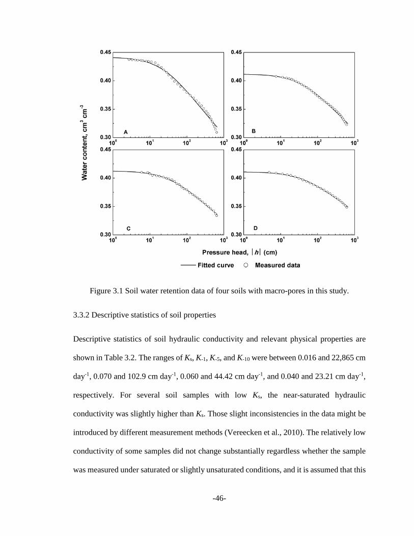
-46-
Figure 3.1 Soil water retention data of four soils with macro-pores in this study.
3.3.2 Descriptive statistics of soil properties
Descriptive statistics of soil hydraulic conductivity and relevant physical properties are
shown in Table 3.2. The ranges of Ks, K-1, K-5, and K-10 were between 0.016 and 22,865 cm
day-1, 0.070 and 102.9 cm day-1, 0.060 and 44.42 cm day-1, and 0.040 and 23.21 cm day-1,
respectively. For several soil samples with low Ks, the near-saturated hydraulic
conductivity was slightly higher than Ks. Those slight inconsistencies in the data might be
introduced by different measurement methods (Vereecken et al., 2010). The relatively low
conductivity of some samples did not change substantially regardless whether the sample
was measured under saturated or slightly unsaturated conditions, and it is assumed that this

-47-
measurement result reflected measurement uncertainty and the absence of macro-pores.
Another explanation could be that soil pores were rinsed out or eroded during the
experiment, since measuring low-permeability soil samples took a long time. For soil
samples with low permeability, the falling head method was used to measure Ks. During
this process, evaporation cannot be completely avoided, which may also cause
underestimation in Ks. The coefficients of variation (CV) indicated that hydraulic
conductivity, especially Ks, was more variable than other physical properties. The high
degree of variation between different soil cores in saturated and near-saturated hydraulic
conductivity was possibly caused by the influence of soil macro-pores. In this no-till soil,
high spatial variation in soil macro-porosity was observed. For instance, macro-porosity
(pores having equivalent diameter larger than 1000 μm) exhibited a CV of 90.7%.
Although, macro-pores account for only a small volume fraction (less than 4% in this
research), they have important influence on soil saturated and near-saturated hydraulic
conductivity (Beven and Germann, 1982) due to their size and geometry (Ehlers et al.,
1995). Two textural classes (silt loam and silty clay loam) were observed in the field
investigated here (Figure 3.2). Silt loam was determined as the predominant soil texture.
The average bulk density was 1.604 g cm-3, while the mean organic matter content was
0.75%. Soil water contents at matric potentials of -100, -330, and -15000 cm had mean
values of 0.408, 0.383, and 0.238 cm3 cm-3, respectively, and the average plant available
water capacity was 0.170 cm3 cm-3.

-48-
Figure 3.2 Textural composition of soils investigated in this study.
Table 3.2 Descriptive statistics for soil hydraulic conductivity and other physical properties over all depths (N= 41).
Variables† Maximum Minimum Mean Geometric mean S.D. ‡ CV, % ‡
Ks, cm day-1 22,865 0.016 662.5 5.094 3572 539 K-1, cm day-1 102.9 0.070 9.256 2.181 19.42 210 K-5, cm day-1 44.42 0.060 4.728 1.263 9.996 211 K-10, cm day-1 23.21 0.040 1.862 0.625 4.223 227
Sand, % 15.69 1.157 4.363 3.588 3.059 70.1 Silt, % 84.05 53.18 71.25 70.91 6.854 9.62 Clay, % 33.94 14.13 24.39 23.76 5.446 22.3 ρb, g cm-3 1.738 1.392 1.604 1.602 0.076 4.74 SOM, % 2.290 0.240 0.751 0.603 0.532 70.8
φ (d ≥1000 μm), % 0.664 0.004 0.158 0.103 0.143 90.7 φ (d ≥75 μm), % 4.002 0.201 1.628 1.316 1.002 61.5 θ-100, cm3 cm-3 0.509 0.366 0.408 0.407 0.025 6.23 θ-330, cm3 cm-3 0.499 0.338 0.383 0.382 0.030 7.74 θ-15000, cm3 cm-3 0.428 0.117 0.238 0.230 0.061 25.7 PAW, cm3 cm-3 0.284 0.081 0.170 0.163 0.047 27.9
† Ks, measured saturated hydraulic conductivity; K-1 K-5 and K-10, hydraulic conductivity at potentials of -1 cm -5 cm and -10 cm; ρb, bulk density; SOM, soil organic matter; φ (d ≥1000 μm) and φ (d ≥75 μm), macro-porosity of pores having equivalent diameter greater than 1000 μm and 75 μm; θ-100 θ-330 and θ-15000, soil water content at potentials of -100 cm -330 cm and -15000 cm; PAW, plant available soil water content.
‡ S.D. standard deviation, CV coefficient of variation (S.D. and CV were computed based on non-transformed data)

-49-
3.3.3 Evaluation of established pedo-transfer functions
The reliability of the most widely used PTFs in estimating Ks at the field scale was
evaluated and compared to locally measured data (Figure 3.3). The predicted Ks values
from the PTFs were weakly related to measured Ks values based on high RMSE, and low
NSE and R2 values. In fact, the predicted Ks values varied by 2 orders of magnitude whereas
measured Ks data varied by 5 orders of magnitude. All PTFs, by their very nature, tend to
smooth data to some degree (Pringle et al., 2007). This might also explain why PTFs
systematically overestimated low measured Ks and underestimated high Ks for this field. In
general, only the mean level (based on log-transformed data) of estimated Ks for PTFs
(except Saxton and Vereecken PTFs) represented the mean (based on log-transformed data)
of measured values (t-test at the 5% significance level) (Figure 3.4). Although it has been
recommended that a given PTF should not be used beyond the geomorphological/pedoclimatic
region or soil type from which it was derived, the differences and similarities between the
development and application datasets in the data range as well as the underlying correlation
patterns have more significant impacts on the reliability of a PTF (Wösten et al., 1997;
Nemes, 2015; Van Looy et al., 2017). In this study, local soil properties are covered by all
databases that were used to derive selected PTFs. In this field where two soil types were
found, the range of soil texture related properties was much narrower than the range
represented in databases that were used for developing PTFs. The variation of Ks was not
sufficiently reflected by the variation of soil texture, bulk density, and organic matter,
which are commonly used to predict Ks in PTFs developed for soils distributed over regions
larger than in this study. Therefore, these texture-dominated PTFs underestimated the
variance of Ks observed in this field due to processes dominant at smaller scales, such as

-50-
soil structure development. It is possible, however, that other soil properties that are
relevant at the given scale might help improve the prediction. The relatively poor Ks
prediction performance might be caused by possible macro-pore effects in the farmland,
since bulk density and organic matter can only partially reflect soil structure (Wagner et
al., 2001). The volume and geometry of large soil pores, which may not be correlated with
the properties of the bulk soil, greatly influence saturated and near-saturated hydraulic
conductivity (Ghafoor et al., 2013). The presence of large pores increases the uncertainty
and complicates the prediction of Ks using published PTFs (Arrington et al., 2013).
Therefore, the established PTFs, in which a macro-pore effect was not considered, might
be suitable for predicting Ks for soil with pore systems dominated by matrix flow, but will
lack precision when applied to structured soils that are influenced by macro-pores (Lin et
al., 1999b). Even inclusion of one or two soil water content points in PTFs like done in
ROSETTA did not improve the prediction of Ks, since water contents at field capacity and
permanent wilting point are decoupled from the macro-pore region. Therefore, the
influence of macro-pores on saturated water flow was further explored.

-51-
Figure 3.3 Measured and estimated saturated hydraulic conductivity, Ks, for the seven
PTF models investigated. (See Table 3.1 for variable definitions.)

-52-
Figure 3.4 Estimated saturated hydraulic conductivity for the field samples on different methods. (Mean ± S.D., number over the symbol is the mean based on non-transformed data, cm day-1)
1-Measured data, 2-Rosetta (sand, silt and clay), 3-Rosetta (sand, silt, clay and ρb), 4-Rosetta (sand, silt, clay, ρb and θ-330), 5-Rosetta (sand, silt, clay, ρb, θ-330 and θ-15000),
6-Cosby et al. 1984, 7-Puckett et al. 1985, 8-Saxton et al. 1986, 9-Vereecken et al. 1990, 10-Wӧsten 1997, 11-Wӧsten et al. 1999.
Hydraulic conductivity at or close to saturation (h ≥ -10 cm) is important to illustrate the
effects of soil macro-pores. A significant drop in hydraulic conductivity is always observed
in soils with macro-pores when pressure head slightly changes in the range near saturation
because these macro-pores drain under even small pressure decrease and do not participate
in water flow anymore (Bouma, 1981). The difference between K measured at saturation
and at h = -10 cm, i.e., Ks - K-10, is therefore considered as macro-pore hydraulic
conductivity (Jarvis et al., 2013). Hydraulic conductivity followed a log-normal
distribution according to the Kolmogorov-Smirnov test at the 5% significance level. The
geometric means for hydraulic conductivity at potentials of 0, -1, -5, and -10 cm were 5.094,
2.181, 1.263, and 0.625 cm day-1, respectively. Based on geometric means, relative
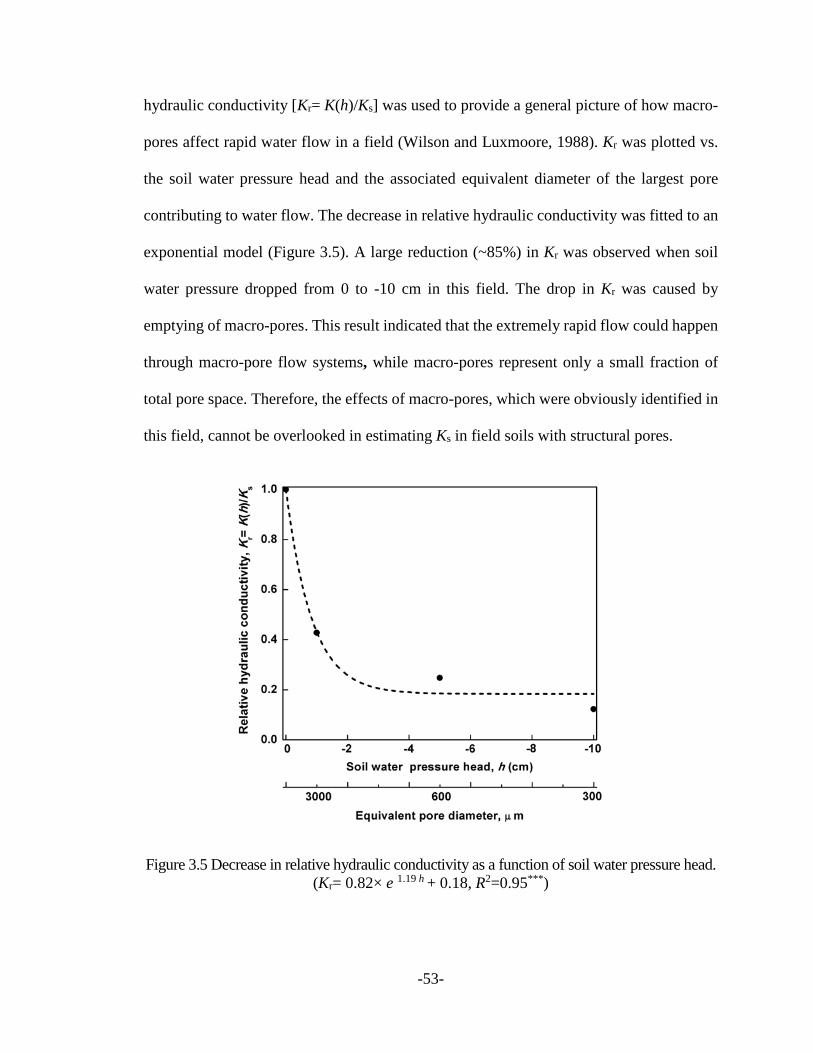
-53-
hydraulic conductivity [Kr= K(h)/Ks] was used to provide a general picture of how macro-
pores affect rapid water flow in a field (Wilson and Luxmoore, 1988). Kr was plotted vs.
the soil water pressure head and the associated equivalent diameter of the largest pore
contributing to water flow. The decrease in relative hydraulic conductivity was fitted to an
exponential model (Figure 3.5). A large reduction (~85%) in Kr was observed when soil
water pressure dropped from 0 to -10 cm in this field. The drop in Kr was caused by
emptying of macro-pores. This result indicated that the extremely rapid flow could happen
through macro-pore flow systems, while macro-pores represent only a small fraction of
total pore space. Therefore, the effects of macro-pores, which were obviously identified in
this field, cannot be overlooked in estimating Ks in field soils with structural pores.
Figure 3.5 Decrease in relative hydraulic conductivity as a function of soil water pressure head. (Kr= 0.82× e 1.19 h + 0.18, R2=0.95***)

-54-
3.3.4 Factors influencing saturated hydraulic conductivity
Before the new PTF was developed, the relationships between measured Ks and other soil
physical properties were investigated. The shape of the soil hydraulic conductivity curve
can be estimated from soil water retention curve parameters. In previous studies, fitted or
optimized van Genuchten (1980) water retention model parameters were successfully used
as predictors of the relative hydraulic conductivity function and then combined with an
estimate of Ks for matching the unsaturated hydraulic conductivity function (Schaap and
Leij, 2000; Minasny et al., 2004). Therefore, the correlations between measured Ks and
water retention curve parameters were also briefly studied in this research. The degree of
linear association of Ks with relevant physical properties was determined using Pearson
correlation analysis (Table 3.3). High positive correlations were found between Ks and silt
content, macro-porosity for pores having diameter larger than 1000 μm [φ (d ≥1000 μm)],
macro-porosity for pores having diameter larger than 75 μm [φ (d ≥75 μm)], and α. Ks was
significantly negatively correlated with clay content, θ-100, θ-330, and θ-15000. Although, sand,
bulk density, and organic matter were widely used as input in some established PTFs
(Vereecken et al., 1990; Wösten et al., 1999), the correlations of Ks with sand, ρb, and SOM
were generally weak in this study probably because the range of variation within our field
site is smaller than the range obtained for large regions. Ks was strongly correlated with
macro-porosity rather than with bulk density which is a proxy for total porosity. This result
is consistent with the observations reported by Ahuja et al. (1984 and 1989), who found
that there was a poor relationship between Ks and total porosity, compared to the
relationship between Ks and macro-porosity (d ≥ 10 μm). It is obvious that macro-pores are
the key in determining rapid water infiltration and drainage in soil, although, total pore

-55-
space remains important (Voroney and Heck, 2015). Ks showing strong positive correlation
with α also confirmed this point. Parameter α is related to the air entry pressure and is an
indicator of soil pore size. Higher α means larger radius of the largest pore in the system
(Schaap and Leij, 2000).
The PCA of fifteen soil physical properties resulted in four PCs, which had eigenvalues
greater than 1 and accounted for 83% of the variance in the measured soil properties (Table
3.4). The first PC explained 37% of the variance. It had high positive loadings on clay
content, soil water content at potentials of -330 cm and -15000 cm, as well as high negative
loading on silt content. Based on Pearson correlation, θ-330, and θ-15000 were significantly
correlated with clay and silt content (p< 0.001). Therefore, PC1 was identified as soil
texture related component. The second PC explained 24% of the variance with high
loadings on φ (d ≥1000 μm), φ (d ≥75 μm), and α. The latter was highly correlated with macro-
porosity (p< 0.001). Thus, PC2 was named as soil structure or macro-porosity component.
The third PC, which was dominated by bulk density only, explained 13% of the variance.
Since bulk density influences soil total porosity, PC3 can be termed as another soil structure
related component. The fourth PC, which was dominated by residual water content (θr),
only explained 9% of the variance. θr is generally influenced by soil texture. For example,
clayey soil usually has higher θr compared with sandy soil (van Genuchten, 1980). PC4
was referred to as another soil texture related component. PCA indicated that the soil
physical properties explaining Ks in the field could be grouped into two dominating factors,
i.e., soil texture and soil structure. Soil structure, especially soil macro-pores, significantly
influence Ks. Soil macro-pores are beneficial in characterizing hydraulic behavior in soils
with structural features (Lin et al., 1999b; Arrington et al., 2013). However, this factor is

-56-
missing in most PTFs, which might explain the unsatisfactory performance of selected
PTFs in estimating Ks when applied to small domains such as our field site with soils that
obviously show structural features of a hierarchical pore space organization (Wagner et al.,
2001; Weynants et al., 2009).
Based on PCA and correlation analysis, silt, clay, θ-330, θ-15000, φ (d ≥1000 μm), φ (d ≥75 μm), and
α were potential predictors in PTF development. Bulk density and organic matter were
thought to be useful predictors for Ks and important in PC3 and PC5 (not shown, because
eigenvalues for PC5-PC15 were less than 1). However, their Pearson correlation
coefficients were not significant. Similar to bulk density and organic matter, residual water
content was important in PC4. However, it had a weak correlation with Ks. These properties
were therefore not considered in the development of a new PTF. The coefficients in a
multiple linear regression model indicate the effect of a predictor on the response after
adjusting for all other predictors in the model. It is possible for a predictor that seems to be
significant in a simple bi-variate linear regression to become non-significant in multiple
linear regression if the effect that variable has on the response is better explained by one or
more of the other variables in the model. This is called multicollinearity, which occurs
when regressing several highly correlated variables. This problem can be solved by
developing a model with fewer independent variables. Therefore, it is crucial to select
proper variables to form a subset of variables for model development. In the first PC, silt,
clay, θ-330 and θ-15000 were important factors, and all the four variables were highly
correlated with each other (p< 0.001). To select variables within this highly correlated
group and reduce redundancy, the absolute values of the bivariate correlation coefficients
for these variables – as the only criterion to select input variables – were summed. The

-57-
variable having the highest sum of absolute correlation coefficients was considered to
represent the group best (Andrews and Carroll, 2001; Wang et al., 2012b). Despite the
approach taken, the selection of representative variables remains somewhat subjective.
There are chances that choosing other representative variables with a similar sum of
correlation coefficients may yield similar results. Based on correlation coefficients, clay
content was considered as the most representative factor of PC1 (Table 3.5). The three
important factors in PC2, i.e., φ (d ≥1000 μm), φ (d ≥75 μm), and α, were also highly correlated (p<
0.001). Since φ (d ≥75 μm) had the highest correlation sum (Table 3.6) and a strong relationship
with Ks, it was considered as the better or more representative factor within PC2.
Considering both Ks and φ (d ≥75 μm) being log-normally distributed (Kolmogorov–Smirnov
test at the 5% significance level), the original data were log-transformed for the
multivariate regression. Thus, clay content and log10 φ (d ≥75 μm) were used as predictors in
the new PTF development.

-58-
Table 3.3 Pearson correlation coefficients between saturated hydraulic conductivity and soil physical properties.
Variable† Ks ρb Sand Silt Clay SOM φ(d ≥1000 μm) φ(d ≥75 μm) θ-100 θ-330 θ-15000 PAW α n θs θr
Ks 1.00
ρb -0.14 1.00
Sand -0.29 -0.15 1.00
Silt 0.54*** -0.13 -0.56*** 1.00
Clay -0.55*** 0.29 0.22 -0.91*** 1.00
SOM 0.19 -0.29 -0.30 0.39* -0.41** 1.00
φ(d ≥1000 μm) 0.43** -0.27 -0.06 0.17 -0.18 -0.20 1.00
φ(d ≥75 μm) 0.55*** -0.37* -0.09 0.27 -0.29 0.00 0.90*** 1.00
θ-100 -0.63*** -0.16 0.30 -0.58*** 0.55*** -0.25 -0.12 -0.28 1.00
θ-330 -0.66*** 0.00 0.32* -0.70*** 0.70*** -0.40* -0.12 -0.32* 0.95*** 1.00
θ-15000 -0.42** 0.28 0.28 -0.78*** 0.82*** -0.58*** -0.02 -0.14 0.56*** 0.70*** 1.00
PAW 0.21 -0.07 -0.28 0.69*** -0.69*** 0.41** -0.01 0.07 -0.49** -0.62*** -0.87*** 1.00
α 0.44** -0.20 -0.02 0.02 0.01 -0.23 0.85*** 0.90*** -0.16 -0.10 0.14 -0.24 1.00
n 0.03 -0.11 -0.08 0.23 -0.24 0.46** -0.63*** -0.31 -0.24 -0.35* -0.32* 0.26 -0.43** 1.00
θs -0.26 -0.49** 0.30 -0.38* 0.30 -0.16 0.32* 0.29 0.81*** 0.70*** 0.40* -0.40* 0.28 -0.30 1.00
θr -0.04 -0.21 0.13 -0.07 0.06 -0.04 -0.39* -0.15 0.02 0.00 0.05 -0.14 -0.09 0.75*** 0.02 1.00
† See Table 3.2 for variable definitions. θr, θs, α, and n are van-Genuchten equation parameters (θr, residual water content; θs, saturated water content; α, related to the inverse of the air-entry pressure head; n, empirical shape parameter).
*, **, *** significant at the 0.05, 0.01, 0.001 probability levels, respectively.

-59-
Table 3.4 Component loadings for soil physical properties and eigenvalues of the principal components (PCs)†.
Soil basic property‡ PC1 PC2 PC3 PC4 Factor loading
ρb 0.10 -0.32 -0.84 0.09 Sand 0.46 -0.04 0.24 0.14 Silt -0.88 0.16 0.04 -0.14 Clay 0.85 -0.17 -0.20 0.14 SOM -0.56 -0.19 0.36 -0.27
φ(d ≥1000 μm) -0.03 0.98 -0.04 0.01 φ(d ≥75 μm) -0.20 0.91 0.16 0.24 θ-100 0.80 -0.09 0.35 -0.41 θ-330 0.90 -0.09 0.16 -0.30 θ-15000 0.90 0.00 -0.20 0.23 PAW -0.80 -0.05 0.03 -0.31 α 0.07 0.88 0.00 0.39 n -0.40 -0.65 0.45 0.39 θs 0.62 0.38 0.58 -0.26 θr 0.02 -0.41 0.54 0.67
Eigenvalue 5.55 3.52 1.97 1.42 Difference 2.03 1.55 0.55 0.49
Variance explained 37% 24% 13% 9%
† The principal components have small variances and eigenvalues (PC5~PC15) were not listed.
‡ See Table 3.2 and Table 3.3 for variable definitions.
Table 3.5 Correlation coefficients and correlation sums for highly weighted variables under first principal component (PC1) with high factor loadings.
PC1 variables† Clay Silt θ-330 θ-15000 Clay - -0.91 0.70 0.82 Silt -0.91 - -0.70 -0.78 θ-330 0.70 -0.70 - 0.70 θ-15000 0.82 -0.78 0.70 -
Correlation sum 2.43 2.39 2.10 2.30
† See Table 3.2 and Table 3.3 for variable definitions.

-60-
Table 3.6 Correlation coefficients and correlation sums for highly weighted variables under second principal component (PC2) with high factor loadings.
PC2 variables† φ(d ≥75 μm) φ(d ≥1000 μm) α φ(d ≥75 μm) - 0.90 0.90 φ(d ≥1000 μm) 0.90 - 0.85
α 0.90 0.85 - Correlation sum 1.80 1.75 1.75
† See Table 3.2 and Table 3.3 for variable definitions.
3.3.5 Pedo-transfer function development
Multiple linear regression analysis was performed to develop the new PTF using clay
content and macro-porosity as predictors. In general, the performance of a PTF is
influenced by the selection of a dataset used to develop the PTF and the validation dataset.
One hundred random realizations were carried out to generate 100 equations to obtain an
information on parameter uncertainties. The distributions of 100 intercepts and 100
coefficients corresponding to each variable are shown in Figure 3.6. Each of the 100
equations was then tested against the corresponding validation dataset to evaluate PTF
reliability. The distributions of evaluation criteria (RMSE, NSE, and R2) are shown in
Figure 3.7. All the distributions were approximately normal (Kolmogorov–Smirnov test at
the 5% significance level).
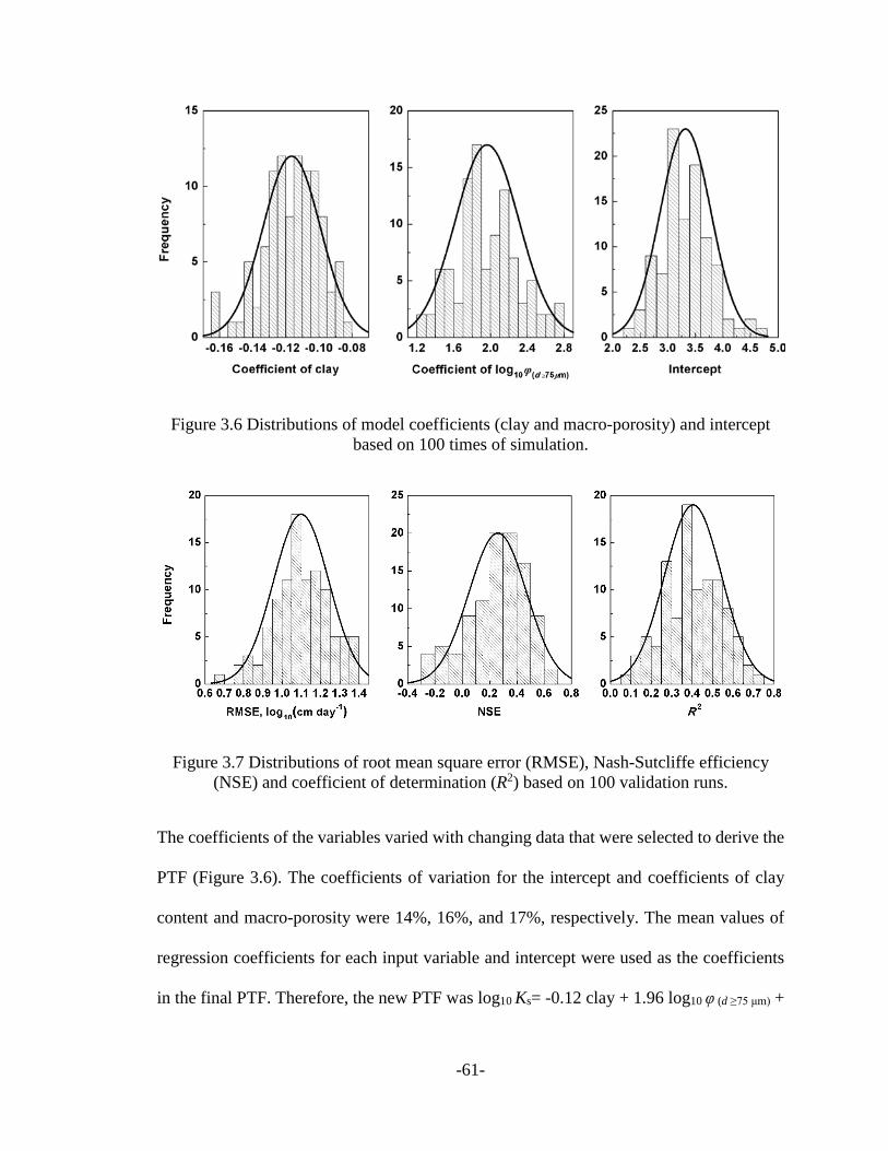
-61-
Figure 3.6 Distributions of model coefficients (clay and macro-porosity) and intercept based on 100 times of simulation.
Figure 3.7 Distributions of root mean square error (RMSE), Nash-Sutcliffe efficiency (NSE) and coefficient of determination (R2) based on 100 validation runs.
The coefficients of the variables varied with changing data that were selected to derive the
PTF (Figure 3.6). The coefficients of variation for the intercept and coefficients of clay
content and macro-porosity were 14%, 16%, and 17%, respectively. The mean values of
regression coefficients for each input variable and intercept were used as the coefficients
in the final PTF. Therefore, the new PTF was log10 Ks= -0.12 clay + 1.96 log10 φ (d ≥75 μm) +

-62-
3.32. Note that a bimodal pattern was identified in each of the graphs in Figure 3.6. This
observation indicated that the averaged coefficients were likely not the most optimal ones
and that this PTF development process still needs further improvements. However, for the
purpose of analysis and comparison in this study, we assumed here that the mean values
were the actual coefficients and used in this PTF. The distributions of RMSE, NSE, and R2
showed that the PTF performance changed significantly for different validation datasets
(Figure 3.7). Increasing the number of realizations from 1 to 100 resulted in variations in
the average regression coefficient of each variable and training error (RMSE) (Figure 3.8).
The average training error generally stabilized with an increasing number of realizations.
A similar trend was also found by Baker and Ellison (2008). When the number of
realizations increased to approximately 70, the training error became stable. For the
regression coefficient of each variable, a significant fluctuation was identified when the
number of realizations was less than 30. When the number of realizations was greater than
40, there was no obvious difference between different numbers of realizations. Therefore,
the results suggest that the regression coefficients of the 100 realizations were sufficient to
generate a stable and reliable PTF in this study. This number of realizations is in agreement
with the results reported by Schaap et al. (2008). Therefore, it was concluded that the
quality of the new PTF greatly depended on the selection of training and validation dataset,
which are highly random for a single realization, especially for relatively small datasets
like ours. Lilly et al. (2008) utilized a resampling technique to derive PTFs showing that
RMSE varied over a wide range using a resampled subset of the same master database. In
our study, it was crucial to repeatedly develop and validate the PTF using a resampling

-63-
method to evaluate the stability of the PTF and obtain a prediction model with relatively
high estimation quality.
Figure 3.8 Average regression coefficient of each variable (left) and training error (right) related to number of realizations.
Although, porosity of macro-pores having a diameter larger than 75 μm was chosen as the
factor representing soil structure and used in the development of new PTF, it is worthwhile
to discuss the influence of different macro-pore delimitations on the performance of PTFs
based on this dataset. Therefore, another PTF using clay and log10 φ (d ≥1000 μm) was derived
using the same method. Both PTFs had similar performance (t-test at the 5% significance
level) while the PTF using macro-pores having diameters larger than 75 μm was slightly
better than the PTF based on macro-pores with diameters larger than 1000 μm (Figure 3.9).
In this local dataset, soil samples were taken from different soil depths. Macro-pores having
diameters greater than 1000 μm, which are mainly earthworm channels or cracks, might be
more pronounced in surface soil than subsoil. Earlier research has found that pores having
a diameter larger than 1000 μm exhibit the most significant influence on Ks. However,
pores having diameters between 75 and 1000 μm still contribute considerably to rapid
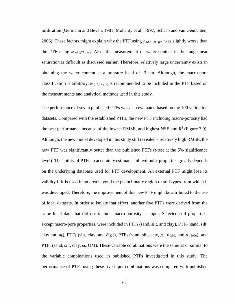
-64-
infiltration (Germann and Beven, 1981; Mohanty et al., 1997; Schaap and van Genuchten,
2006). These factors might explain why the PTF using φ (d ≥1000 μm) was slightly worse than
the PTF using φ (d ≥75 μm). Also, the measurement of water content in the range near
saturation is difficult as discussed earlier. Therefore, relatively large uncertainty exists in
obtaining the water content at a pressure head of -3 cm. Although, the macro-pore
classification is arbitrary, φ (d ≥75 μm) is recommended to be included in the PTF based on
the measurements and analytical methods used in this study.
The performance of seven published PTFs was also evaluated based on the 100 validation
datasets. Compared with the established PTFs, the new PTF including macro-porosity had
the best performance because of the lowest RMSE, and highest NSE and R2 (Figure 3.9).
Although, the new model developed in this study still revealed a relatively high RMSE, the
new PTF was significantly better than the published PTFs (t-test at the 5% significance
level). The ability of PTFs to accurately estimate soil hydraulic properties greatly depends
on the underlying database used for PTF development. An external PTF might lose its
validity if it is used in an area beyond the pedoclimatic region or soil types from which it
was developed. Therefore, the improvement of this new PTF might be attributed to the use
of local datasets. In order to isolate that effect, another five PTFs were derived from the
same local data that did not include macro-porosity as input. Selected soil properties,
except macro-pore properties, were included in PTF1 (sand, silt, and clay), PTF2 (sand, silt,
clay and ρb), PTF3 (silt, clay, and θ-330), PTF4 (sand, silt, clay, ρb, θ-330, and θ-15000), and
PTF5 (sand, silt, clay, ρb, OM). These variable combinations were the same as or similar to
the variable combinations used in published PTFs investigated in this study. The
performance of PTFs using these five input combinations was compared with published

-65-
PTFs and the local PTF that included macro-porosity as input. Figure 3.9 shows that the
estimation of Ks using PTF1, PTF2, PTF3, PTF4, and PTF5 was no better than the prediction
by some widely used established PTFs derived from the same or similar input combinations
(t-test at the 5% significance level). However, the new PTF including macro-porosity
performed significantly better than PTF1, PTF2, PTF3, PTF4, and PTF5 (t-test at the 5%
significance level). These results confirm that although using a local dataset may play a
role in improving the performance of a new PTF, soil macro-porosity was the crucial
component that greatly improved the performance of the new PTF. Therefore, the PTF,
which was developed based on a small but relevant dataset and which took the effect of
macro-pore volume on Ks into account, was more suitable in estimating Ks for different
locations within a specific field than for any of the examined existing PTFs that did not
account for macro-porosity. Soil textural properties were not sufficient to compensate for
the lack of information on macro-porosity to predict Ks in this field with structured soil.

-66-
Figure 3.9 The performance of pedo-transfer functions based on 100 validation runs. (Box and Whisker plots show the mean, 1st, 25th, 50th, 75th and 99th percentile of the distributions.) 1-New PTF (clay and log10 φ[d ≥75 μm]), 2-New PTF (clay and log10 φ[d ≥1000 μm]), 3-PTF1 (sand, silt, and clay), 4-PTF2 (sand, silt, clay and ρb), 5-PTF3 (silt, clay, and θ-330), 6-PTF4 (sand, silt, clay, ρb, θ-330, and θ-15000), 7-PTF5 (sand, silt, clay, ρb, OM), 8-Rosetta (sand, silt and clay), 9-Rosetta (sand, silt, clay and ρb), 10-Rosetta (sand, silt, clay, ρb and θ-330), 11-Rosetta (sand, silt, clay, ρb, θ-330 and θ-15000), 12-Cosby et al. 1984, 13-Puckett et al. 1985, 14-Saxton et al. 1986, 15-Vereecken et al. 1990, 16-Wӧsten 1997, 17-Wӧsten et al. 1999.
3.4 Conclusions
In this study, local measurements taken from a farmer’s field were used to evaluate the
performance of established PTFs in estimating Ks in a specific site. The strong spatial
variation of measured Ks, which was caused by the presence of macro-pores, observed in
-67-
the field was not reflected by the predicted values. These classical PTFs, which utilize
particle-size distribution, dry bulk density, and organic matter as predictors, should be used
with caution and their limitations discussed in this study should be kept in mind when
predicting the spatial variability of Ks at the field scale. Principal component analysis and
correlation analysis were performed to identify the influencing factors of Ks in the field.
Fifteen variables were grouped into two most influencing components (soil texture related
component and macro-pore component), which explained more than 60% of the variance.
Clay content and macro-porosity for pores having diameters larger than 75 μm were
selected to represent each component and used as predictors in the new PTF. The new PTF,
which was developed by multiple linear regression, performed much better compared with
established PTFs tested in this study. This finding indicated that taking soil macro-pore
effects into account improved the prediction of Ks. The selection of calibration-validation
data subsets also impacted PTF performance, therefore resampling and subsequent
uncertainty analysis was necessary during the PTF development process.
The ability of PTFs to accurately predict soil properties often greatly depends on the
underlying data. The pedoclimatic region, soil types, as well as land use and management
practices in this field do not vary or vary within a narrow range. Therefore, similarly to
many PTFs that were developed for specific regions, the new PTF presented in this research
should be applied to other fields with great caution and needs validation in other domains.
Furthermore, an important aim of this study was to improve the estimation of Ks with PTFs
at the field scale by taking into account soil structural information, such as macro-porosity.
For the advancement of knowledge, this research highlighted the importance of soil
structural information in characterizing soil hydraulic properties and proved that including

-68-
soil structural pores information in PTFs improved the estimation of Ks. However, an
effective means of quantifying soil structural information remains elusive. It was difficult
to either quantify soil macro-porosity or identify macro-pores effects by measuring soil
near saturated hydraulic conductivity. With the development of novel indirect
measurement or imaging techniques, quantitative soil structural information will
increasingly become available. The benefit of using quantitative soil structural information
in PTFs should be widely pursued in the future.
Copyright © Xi Zhang 2019

-69-
Chapter 4 Estimating soil hydraulic conductivity at the field scale with a state-space modeling approach
4.1 Introduction
Quantification of soil hydraulic properties is vitally important for understanding and
describing water/solute transport in the soil, which are essential for the management of
surface-applied water and agrochemicals as well as improvement of crop production (Yang
and Wendroth, 2014; Qiao et al., 2018a). Saturated hydraulic conductivity (Ks) is one of
the most important hydraulic properties influencing water/solute movement through soil
under saturated condition. In addition, Ks coupled with more easily measured soil water
retention function is often used to predict unsaturated hydraulic conductivity, since the
complete unsaturated hydraulic conductivity function is difficult to measure directly (van
Genuchten and Nielsen, 1985). However, Ks is sensitive to structural macropores (e.g., bio-
pores created by plant root and fauna activity), and might be completely unrelated with
hydraulic conductivity under unsaturated condition [K(h)] (Schaap and Leij, 2000; Wuest,
2001; Libohova et al., 2018). Therefore, using Ks as a matching point might overestimate
unsaturated hydraulic conductivity since unsaturated water flow takes place in the soil
matrix (Schaap and Leij, 2000). Although the effects of macropores on water flow can be
identified until matric potential of about -40 cm, the contribution of macropores to the
hydraulic conductivity is most significant when matric potential is above -10 cm (Schaap
and van Genuchten, 2006; Jarvis, 2007; Weynants et al., 2009). By excluding the
substantial effects of macropores, using hydraulic conductivity under slightly unsaturated
condition would provide more reliable estimations of unsaturated hydraulic conductivity
(Schaap and Leij, 2000; Jarvis et al., 2002). The hydraulic conductivity at a matric potential

-70-
of -10 cm is recommended to be used as a matching point and defined as saturated matrix
hydraulic conductivity (Jarvis et al., 2002). Hydraulic conductivity exhibits highly spatial
variability at the field scale mainly due to the heterogeneity in soil physical characteristics
(Ersahin, 2003). Therefore, knowledge of the spatial variability of saturated hydraulic
conductivity (Ks) and matrix saturated hydraulic conductivity (K-10) is critical in describing
field-scale water/solute flow processes in both the macropores and the soil matrix pores.
Accurate assessment of spatial variability of soil hydraulic conductivity requires a large
number of soil samples and therefore can only be conducted for limited areas (Comegna et
al., 2010). To overcome this limitation, more attention has been attracted to using more
easily available soil properties (e.g., soil texture, organic matter and bulk density) as a basis
for estimating hydraulic conductivity and characterizing its spatial variability (Wösten et
al., 2001; Ferrer Julià et al., 2004; Montzka et al., 2017). There are many methods (e.g.,
stepwise multiple linear regression and artificial neural network) that can be used to
quantify the relationship between the variable of interest and its influencing factors. Linear
regression is the most commonly used method in developing prediction models for
hydraulic conductivity (Merdun et al., 2006; Wang et al., 2012a; Zhao et al., 2016).
However, linear regression modeling ignores the spatial dependence of variables and
thereby often generates unsatisfied results (Nielsen and Alemi, 1989).
During the last three decades, state-space modeling approach has been used to analyze spatial
series of soil data (Morkoc et al., 1985). State-space modeling considers the spatial
dependences between variables. In an autoregressive state-space model, the variable of
interest is related to the same and a set of other variables at the previous location(s), and the
regression coefficient of each variable reflects its contribution to the estimate (Nielsen and

-71-
Wendroth, 2003; Yang and Wendroth, 2014). Using autoregressive state-space model,
Morkoc et al. (1985) successfully described the spatial relationship between soil water content
and soil temperature. Timm et al. (2004) quantified the spatial correlations between soil
physical and chemical properties with state-space model. Wendroth et al. (2006) utilized state-
space model to investigate the spatial association of soil hydraulic properties, soil texture, and
geoelectrical resistivity. State-space model was also successfully used in estimating soil
organic carbon contents based on silt content and bulk density (Liu et al., 2012). State-space
modeling has been demonstrated to be a more effective method for analyzing the spatial
relationships among variables compared with the equivalent linear regression equations (Jia
et al., 2011; She et al., 2014; Duan et al., 2016). However, few state-space models of hydraulic
conductivity at and near saturation have been developed and presented (Qiao et al., 2018a).
To this end, the objectives of this study were (1) to determine the spatial patterns of hydraulic
conductivity, and quantify the relationships between hydraulic conductivity and other soil
properties by a state-space model; (2) to evaluate the performance of transition coefficients
obtained from state-space models in ordinary autoregressive models without any stochastic
filtering and updating; and (3) to compare the results obtained from state-space approach with
pedo-transfer functions based on classical linear regression.
4.2 Materials and Methods
4.2.1 Site description and soil sampling
This research was conducted in a farmland (~30 ha) located in Caldwell County, Kentucky,
United States (37°1′42″-37°1′58″N, 87°51′11″-87°51′33″W) (Figure 4.1). At this area, the
mean annual precipitation is 1300 mm with a mean annual temperature of 15 °C (US
Climate Data, 2016). Wheat/ double-crop soybean/ corn rotation is practiced in this field.

-72-
Undisturbed soil cores were sampled in a 71 m by 71 m grid of 48 locations from 7-13 cm
depth by using cutting rings (diameter: 8.4 cm, height: 6 cm, volume: 332 cm3). Soil cores
were used to measure saturated and near-saturated hydraulic conductivity, soil water
retention at the wet range, and bulk density. Disturbed soil samples were air-dried and
passed through a 2-mm sieve for other soil physical property analyses.
Figure 4.1 Sampling grid and array of data for state-space modeling.
4.2.2 Laboratory analysis
Soil texture was determined by the sieving and the pipette method (Gee and Or, 2002).
According to USDA textural classification, three textural classes (silt, silty loam and silty clay
loam) were observed in the field. Silty loam was determined as the predominant soil texture.
The core method was used to measure bulk density (ρb) (Grossman and Reinsch, 2002). Soil
organic matter (SOM) was measured by the combustion method (Nelson and Sommers, 1982).
Saturated hydraulic conductivity (Ks) was determined using a permeameter (Eijkelkamp,
Netherlands) based on Darcy’s law under constant and falling head conditions depending
on the individual percolation rate of each sample (Klute and Dirksen, 1986). Hydraulic

-73-
conductivity at a potential of -10 cm (K-10) was measured with a self-developed double
pressure plate-membrane apparatus with two tension plates at the upper and lower end of
the soil core, which are similar to those used with tension infiltrometers (Wendroth and
Simunek, 1999). The computation of K(h) was based on Buckingham-Darcy’s law.
Soil macro-pores have a significant impact on saturated and near-saturated water flow, and
are important to predict hydraulic conductivity at and near saturation (Jarvis et al., 2002;
Vereecken et al., 2010; Arrington et al., 2013). Soil macro-porosity (φ) was therefore
measured in this study. Soil pore diameter (d, μm) can be associated with pressure head (h,
cm) with the equation of d=3000/ǀhǀ (Hillel, 1980). Soil macro-porosity can be measured
from the volume of water drained between saturation and a certain potential (McIntyre and
Sleeman, 1982). The classification of macro-pore size is arbitrary (Allaire et al., 2009).
According to different researchers, equivalent diameters larger than 1000, 80, 75, 60, and
10 μm were considered as macro-pores (Luxmoore, 1981; Bouma, 1991; Singer and Munns,
2002; Vereecken et al., 2010; Arrington et al., 2013; Voroney and Heck, 2015; Weil and
Brady, 2016). In the present study, soil water content at potential of -50 cm was measured
with a pressure plate apparatus (Soilmoisture, CA). Therefore, diameter of 60 μm was
considered as delimitation of macro-pores. As a proximate approach, macro-porosity (φ)
was calculated by φ = θs- θ (h= -50cm) (θs is the saturated soil water content, cm3 cm−3).
4.2.3 Theory of state-space modeling
As state-space analysis is designed for observations taken in one dimension, the
experimental data sampled across the field was arrayed in a spatial series (beginning in the
upper right-hand corner of the field and leading to the lower right-hand corner of the field)
that allows the application of state-space analytical tools (Figure 4.1). Although the spatial

-74-
direction of data series was certainly changed, spatial distances remain as if observations
were taken along one line with regular sampling intervals (Wendroth et al., 2003).
The autoregressive state-space model, which consists of a state equation and an observation
equation, describes how the state of the variable of interest at the ith location is correlated
with the state of the same variable and other related variables at the (i – 1)th location
(Nielsen and Wendroth, 2003; Qiao et al., 2018b). In a commonly used first-order
autoregressive state-space model, the state equation is described as
Zi = ΦZi-1 + ωi (4.1)
where Zi is the state vector (of a set of p variables) at the ith location, Φ is a 𝑝𝑝 × 𝑝𝑝 transfer
matrix consisting of autoregression coefficients, and ωi is uncorrelated zero mean model
error vector with a common q × q covariance matrix Q. Units of Q are variance per length
in space, and depend on the interval between observations.
The state equation is solved simultaneously with the observation equation, which is
described as
Yi = MiZi + υi (4.2)
the observation vector Yi is associated with the true state vector Zi through a measurement
matrix Mi and an uncorrelated zero mean measurement error vector υi. The observation
vector, Yi, does not represent the real state but is only an indirect reflection of the state. The
state-space model, in this study, was solved using Kalman filtering (Kalman, 1960) and the
expectation maximization algorithm (Shumway and Stoffer, 1982) within an iterative
procedure, during which the iteration was terminated once the relative convergence limit
of 0.005 was reached.

-75-
To remove differences in magnitude, it is necessary to scale the data before state-space
analysis. When the variables are in the same order of magnitude, their relative contributions
to the estimate are reflected in their transition coefficients in the corresponding state-space
model. The relative contribution of each variable can be calculated by dividing the
corresponding transition coefficient over the sum of coefficients in the respective equation
(Nielsen and Wendroth, 2003; Yang and Wendroth, 2014). The scaling procedure can be
performed by the following equation
xi' = 𝑥𝑥𝑖𝑖−(�̅�𝑥−2𝜎𝜎)4𝜎𝜎
(4.3)
where xi' is the scaled value, xi is the measured value, �̅�𝑥 is the mean value, and σ is the
standard deviation. The scaled data series have a mean of 0.5 and a standard deviation of
0.25. In this study, all the hydraulic conductivity data was log-transformed prior to being
scaled by equation (4.3).
In order to evaluate the resulting transition coefficients from state-space analysis, these
coefficients were applied in simple autoregressive models, where only the first hydraulic
conductivity (K) in the data series is known, and all following values are predicted from the
previous one and those from the underlying variables included in the corresponding state
vector. The average of squared deviations (SQDavg) between measured hydraulic conductivity
(Kmea) and estimated hydraulic conductivity (Kest) was calculated with equation (4.4) before
the updating step and used as a criterion for prediction quality (Wendroth et al., 2003).
SQDavg = 1𝑛𝑛∑ (𝐾𝐾mea − 𝐾𝐾est)2𝑛𝑛𝑖𝑖=1 (4.4)
in which n is the number of observations.

-76-
4.3 Results and discussion
The spatial distribution of soil hydraulic conductivity across the 48 locations arrayed in
one dimension is shown in comparison to sand content, silt content, clay content, bulk
density (ρb), soil organic matter (SOM), and macro-porosity (φ) (Figure 4.2). Although
several extreme values were identified in the field, sand, silt, clay, bulk density and organic
matter were relatively more stable compared with soil hydraulic conductivity (Table 4.1).
Ks values ranged from 0.02 to 16307 cm day-1, while K-10 values ranged from 0.04 to 5.66
cm day-1. Both Ks (CV= 286%) and K-10 (CV= 91%) had strong variation throughout the
field. At the small research scale of a farmer’s field, wet-range hydraulic conductivity is
rather sensitive to soil structure, which is strongly influenced by extrinsic variations (e.g.,
biological activity, agricultural management) (Jarvis et al., 2002; Zeleke and Si, 2005). In
this no-till soil, high variation (CV= 67%) in soil macro-porosity, which is an indirect
indicator for soil structure, was also observed. This might explain the strong variation in
hydraulic conductivity.
Table 4.1 Descriptive statistics for soil hydraulic conductivity and basic soil properties over the field (N= 48).
Variables † Maximum Minimum Mean S.D. ‡ CV, % ‡ Skewness Ks, (cm day-1) 16307 0.02 983 2815 286 4.02
K-10, (cm day-1) 5.66 0.04 1.20 1.09 91 1.92 Sand, % 11 2 4 1 32 2.36 Silt, % 85 57 79 6 7 -1.88 Clay, % 33 10 17 5 29 1.38 ρb, g cm-3 1.77 1.33 1.61 0.07 4 -1.37 SOM, % 2.38 0.70 1.38 0.31 22 0.59 φ, % 6.51 0.41 2.04 1.36 67 1.46
†Ks, saturated hydraulic conductivity; K-10, hydraulic conductivity at potential of -10 cm; ρb, bulk density; SOM, soil organic matter; φ, macro-porosity.
‡ S.D., standard deviation; CV, coefficient of variation.

-77-
Figure 4.2 Spatial distributions of soil hydraulic conductivity and physical properties
across the field.
Pearson’s correlation analysis was conducted to determine the strengths of the linear
associations between the hydraulic conductivity and other soil physical properties (Table
4.2). K-10 was positively correlated with the silt content, but negatively correlated with clay
content and bulk density. Although, sand, silt, clay, bulk density, and organic matter were
widely used as input in some established PTFs to estimate Ks (Wösten et al., 1999), the
correlations of Ks with these properties were generally weak in this study probably because
the variation of these properties within this field site is small. Both Ks and K-10 were
significantly correlated with the macro-porosity, thereby indicating the importance of
macro-porosity for the spatial distribution of hydraulic conductivity. Variables that
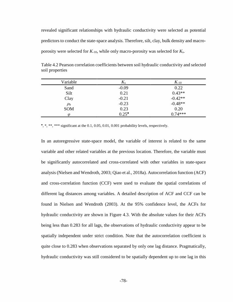
-78-
revealed significant relationships with hydraulic conductivity were selected as potential
predictors to conduct the state-space analysis. Therefore, silt, clay, bulk density and macro-
porosity were selected for K-10, while only macro-porosity was selected for Ks.
Table 4.2 Pearson correlation coefficients between soil hydraulic conductivity and selected soil properties
Variable Ks K-10 Sand -0.09 0.22 Silt 0.21 0.43** Clay -0.21 -0.42** ρb -0.23 -0.48**
SOM 0.23 0.20 φ 0.25● 0.74***
●, *, **, *** significant at the 0.1, 0.05, 0.01, 0.001 probability levels, respectively.
In an autoregressive state-space model, the variable of interest is related to the same
variable and other related variables at the previous location. Therefore, the variable must
be significantly autocorrelated and cross-correlated with other variables in state-space
analysis (Nielsen and Wendroth, 2003; Qiao et al., 2018a). Autocorrelation function (ACF)
and cross-correlation function (CCF) were used to evaluate the spatial correlations of
different lag distances among variables. A detailed description of ACF and CCF can be
found in Nielsen and Wendroth (2003). At the 95% confidence level, the ACFs for
hydraulic conductivity are shown in Figure 4.3. With the absolute values for their ACFs
being less than 0.283 for all lags, the observations of hydraulic conductivity appear to be
spatially independent under strict condition. Note that the autocorrelation coefficient is
quite close to 0.283 when observations separated by only one lag distance. Pragmatically,
hydraulic conductivity was still considered to be spatially dependent up to one lag in this

-79-
study. The ACF results indicated that hydraulic conductivity should be sampled at closer
intervals to obtain more spatial information.
Figure 4.3 Autocorrelation functions (ACF) for soil hydraulic conductivity.
The spatial cross-correlations differed in various directions as well as the lags between
hydraulic conductivity and selected variables according to the results of the CCF analysis
(Figure 4.4). K-10 was significantly cross-correlated with silt and clay contents up to only
one lag. Cross-correlograms also indicated a strong spatial dependence between macro-
porosity and hydraulic conductivity up to one lag. However, there was no significant cross-
correlation between K-10 and bulk density. Therefore, bulk density was removed from the
subsequent state-space analysis. The results obtained from the cross-correlation functions
showed that it was possible for the selected variables (i.e., silt, clay and φ) to be used to
describe soil hydraulic conductivity in the first-order autoregressive state-space analysis.

-80-
Figure 4.4 Cross-correlation functions (CCF) for soil hydraulic conductivity and physical properties.
The state-space model quantified the relationships between soil hydraulic conductivity and
other variables in the neighborhood. The state-space equations for different variable
combinations as well as their coefficient of determination (R2) are shown in Table 4.3. In
order to evaluate the results, the state-space models with the best performance for Ks and
K-10 were tested in two different scenarios (using all the hydraulic conductivity
measurements and 50% of the hydraulic conductivity measurements).

-81-
Table 4.3 State-space analysis of soil hydraulic conductivity using silt, clay, and macro-porosity.
No. State-space model SQDavg R2 M1 (Ks)i = 0.379 (Ks)i-1 + 0.598 (φ)i-1 + ωi 0.019 0.69 M2 (K-10)i = 0.087 (K-10)i-1 + 0.857 (silt)i-1 + ωi 0.006 0.90 M3 (K-10)i = 0.734 (K-10)i-1 + 0.246 (clay)i-1 + ωi 0.018 0.71 M4 (K-10)i = 1.444 (K-10)i-1 – 0.521 (φ)i-1 + ωi 0.020 0.69 M5 (K-10)i = 0.029 (K-10)i-1 + 0.725 (silt)i-1 + 0.236 (clay)i-1 + ωi 0.002 0.96 M6 (K-10)i = 0.093 (K-10)i-1 + 0.617 (silt)i-1 + 0.230 (φ)i-1 + ωi 0.011 0.82 M7 (K-10)i = 0.587 (K-10)i-1 + 0.392 (clay)i-1 – 0.002 (φ)i-1 + ωi 0.005 0.92 M8 (K-10)i = -0.339 (K-10)i-1 + 0.696 (silt)i-1 + 0.167(clay)i-1
+0.466(φ)i-1+ ωi 0.001 0.98
Figure 4.5 Bivariate state-space analysis of saturated hydraulic conductivity (Ks) and macro-porosity (φ) using all Ks observations (a) and 50% of the Ks observations (b), respectively.
The 95% confidence interval limits of estimation are displayed in both cases.
For Ks, the bivariate state-space model equation included macro-porosity (M1) had an R2
value of 0.69. The neighboring Ks contributed about 40% to the estimated value.

-82-
Nevertheless, the majority of the estimated value (~60%) was derived from the strong
spatial cross-correlation between Ks and macro-porosity. The general trend of Ks across the
field was well captured by the state-space model (Figure 4.5a). When 50% of the Ks
observations were not considered for the estimation, the coefficients in the equation
changed considerably (Figure 4.5b). This implied that the weights of different variables
that contribute to the estimation are depended on the available data (Wendroth et al., 2001).
In the second scenario, some of the measured values of Ks fell outside the area of the 95%
confidence interval, and the value of R2 was only 0.41. When using 50% of the data, the
contribution from neighboring Ks to the estimate of Ks significantly increased to about 60%.
Excluding half of the measured data is therefore worsened the prediction of Ks with state-
space model. Note that the width of the 95% confidence interval was slightly narrower in
the second scenario. In addition, the spatial process of Ks was rather smooth in the second
scenario, which means local fluctuations cannot be preserved when 50% of the
measurements were removed. These results might be explained by the omission of some
extremely high and low values (Wendroth et al., 2003).
When all variables were used (M8), the state-space analysis provided an extremely accurate
estimate of the observed K-10 distribution (Figure 4.6a). Note in this case, the neighboring
K-10 contributed about 20% to the estimate of K-10. Excluding silt content in the analysis
(M7) substantially increased the contribution of the neighboring K-10 (~60%) to the estimate
of K-10, and excluding silt and clay contents (M4) further increased the contribution of the
neighboring K-10 to about 73%. In addition, the value of the neighboring K-10 contributed
very little (less than 5%) to the estimate of K-10 in M5, which included only silt and clay
contents. These results indicated that the cross-correlations between K-10 and soil texture

-83-
were sufficiently strong to estimate K-10 with little contribution from the K-10 neighbor
(Figure 4.7a). Therefore, both M5 and M8 were considered as models with the best
performance in this study and further tested in two different scenarios.
Figure 4.6 Multivariate state-space analysis of near-saturated hydraulic conductivity (K-10), silt content, clay content, and macro-porosity (φ) using all K-10 observations (a) and 50% of the K-10 observations (b), respectively. The 95% confidence interval limits of estimation
are displayed in both cases.
In general, the spatial pattern of K-10 across the field was well captured by both state-space
models in the two different scenarios (Figure 4.6 and 4.7). In both scenarios, the
contributions of the neighboring variables in M5 and M8 to the estimate of K-10 remained
relatively stable. Note that the 95% confidence interval of the estimation slightly increased

-84-
in the second scenario (Figure 4.6b and 4.7b), where less observations of hydraulic
conductivity became available for updating.
Figure 4.7 Multivariate state-space analysis of near-saturated hydraulic conductivity (K-10),
silt content, and clay content using all K-10 observations (a) and 50% of the K-10 observations (b), respectively. The 95% confidence interval limits of estimation are
displayed in both cases.
Note that the hydraulic conductivity measurements had to be included in the state-space
estimation procedure in order to determine underlying processes. However, direct
measurements of hydraulic conductivity are often arduous, time-consuming, and expensive
(Wösten et al., 2001). We are interested in how well the results from state-space analysis
can be applied to a scenario that the hydraulic conductivity data is not available. Therefore,
the transition coefficients from state-space equations obtained above (Figure 4.5, 4.6 and

-85-
4.7) were further evaluated through application in ordinary autoregressive models, where
only the initial hydraulic conductivity value at position 1 is available.
Autoregressive Ks predictions were based on transition coefficients obtained from two
different scenarios above (Figure 4.5a and b). The average squared deviation (SQDavg)
between prediction and observation is 0.065 if transition coefficients were based on the
scenario using all observations, and 0.062 if transition coefficients were based on the
scenario with only 50% of the observations, respectively. Both scenarios have similar
prediction quality. Although the precise estimation of Ks magnitude was unsatisfied, the
relative spatial process of Ks was obtained from this autoregressive prediction (Figure 4.8).
Figure 4.8 Autoregressive prediction of saturated hydraulic conductivity (Ks), based on Ks and macro-porosity (φ). Autoregression coefficients were obtained from state-space
analysis (Figure 4.5).

-86-
Autoregressive K-10 predictions based on transition coefficients obtained from state-space
analysis in Figure 4.6 and 4.7 were shown in Figure 4.9 and 4.10, respectively. According
to SQDavg, all the four autoregressive prediction procedures exhibited similar prediction
quality. In general, the spatial pattern of K-10 was well captured by this autoregressive
prediction (Figure 4.9 and 4.10), although the magnitudes of K-10 at several points were not
predicted accurately. Results from the autoregressive prediction of K-10 are encouraging.
K-10 is commonly recommended to be used as a matching point for the unsaturated
hydraulic conductivity function. Therefore, an accurately spatial characterization of K-10
can still be useful for studying soil water flow.
Figure 4.9 Autoregressive prediction of near-saturated hydraulic conductivity (K-10),
based on K-10, silt content, clay content, and macro-porosity (φ). Autoregression coefficients were obtained from state-space analysis (Figure 4.6).

-87-
Figure 4.10 Autoregressive prediction of near-saturated hydraulic conductivity (K-10), based on K-10, silt content, and clay content. Autoregression coefficients were obtained
from state-space analysis (Figure 4.7).
Moreover, the state-space models were compared with multiple linear regression models.
The multiple linear regression analysis results for different combinations of variables are
shown in Table 4.4. It should be noted that all the classical linear models were developed
on scaled data series and all the data passed Kolmogorov-Smirnov test for normality (at
the 5% significance level). The variables related to the best performance for K-10 were
similar to those determined by the state-space analysis. Namely, for classic linear
regression analysis and state-space analysis, the model including both soil textural (silt and
clay) and structural information (macro-porosity) has the best performance. State-space
modeling described the spatial relationship between hydraulic conductivity and soil
physical properties much better than classic linear regression analysis. The autoregressive

-88-
state-space approach takes advantage of the spatial correlation inherent in observations and
analyzes how the change in one variable from one location to the next is related to the
change in the other variables. The classical regression analysis, on the contrary, is based on
the assumption that all the observations are independent from each other and ignores the
local spatial cross-correlations between variables within the field. Therefore, classic
regression analysis often fails at the field scale due to the measurements are usually spatially
correlated (Nielsen and Alemi, 1989; Timm et al., 2004; Yang and Wendroth, 2014).
Table 4.4 Linear regression analysis of soil hydraulic conductivity using silt, clay, and macro-porosity.
Linear regression model SQDavg R2 Ks = 0.374 + 0.252 (φ) 0.059 0.06 K-10 = 0.287 + 0.427 (silt) 0.051 0.18 K-10 = 0.708 – 0.416 (clay) 0.052 0.17 K-10 = 0.131 + 0.738 (φ) 0.028 0.54 K-10 = 0.295 + 0.419 (silt) – 0.009 (clay) 0.051 0.18 K-10 = 0.048 + 0.234 (silt) + 0.671 (φ) 0.025 0.59 K-10 = 0.281 – 0.238 (clay) + 0.675 (φ) 0.025 0.60 K-10 = 0.258 + 0.024 (silt) – 0.215 (clay) + 0.675 (φ) 0.025 0.60
In the bivariate linear regression, the model including macro-porosity alone had good
performance (R2 = 0.54) in estimation of K-10 and adding soil texture to the model only
slightly improved the prediction (R2 = 0.60). However, the state-space model including soil
texture alone (M5) had sufficient accuracy in estimating K-10 and adding macro-porosity
(M8) to the model only improved the performance marginally. Unlike classic regression
analysis, the strongest contributing variable that was identified in state-space analysis was
soil texture. The results from state-space analysis are promising, since soil texture is an
easily measured property, while soil structural information is more difficult to characterize.
-89-
However, the validity of the state-space models presented in this study have to be further
examined in other fields.
4.4 Conclusions
Knowledge of the spatial variability of saturated hydraulic conductivity (Ks) and matrix
saturated hydraulic conductivity (K-10) is critical in describing field-scale water flow
processes. This study investigated the spatial distributions of hydraulic conductivity, and
quantified the spatial relationship between hydraulic conductivity and its potential
influencing factors by using a state-space approach at the field scale. All the state-space
models well described the spatial characteristics of hydraulic conductivity and results
obtained from ordinary autoregressive models are encouraging. Due to the sampling interval,
spatial autocorrelations were not high for hydraulic conductivity. Future work should focus
on the effect of sampling density on state-space modeling in terms of variables that are
included in the model and the model accuracy. Compared to ordinary correlation analysis,
state-space analysis resulted in a different answer which variables were helpful in estimating
K-10. Unlike classic regression analysis, the strongest contributing variable that was identified
in state-space analysis was soil texture. Moreover, all the derived state-space models
described the relationships between hydraulic conductivity and other variables better than
the equivalent linear regression models. Although the state-space models developed in this
study need to be further validated in other fields, the state-space approach proved to be a
more effective tool for better describing the spatial variability of hydraulic conductivity.
Copyright © Xi Zhang 2019

-90-
Chapter 5 Conclusions
Knowledge of the spatial variability of hydraulic conductivity at and near saturation is
critical in describing field-scale water flow processes and important for improving field
water management. The research presented in this dissertation attempted to validate and
improve the application of PTFs to estimate the spatial variability of hydraulic conductivity
at the field scale.
The spatial variability of wet range hydraulic conductivity in a no-till farmland was
characterized with geostatistical techniques and compared with the spatial variability
obtained from PTFs estimates. Owing to the presence of structural macro-pores, Ks showed
high spatial heterogeneity and this variability was not captured by PTF estimates. However,
the general spatial pattern of near-saturated hydraulic conductivity can still be reasonably
generated by PTF estimates. These classical PTFs in which soil structural information was
not included should be used with caution when studying the spatial variability of Ks at the
field scale.
In the studied field site, macro-pore effects were predominant and had a great contribution
to saturated water flow. Therefore, PTFs were further improved by including soil macro-
porosity and had been proven to perform much better compared with established PTFs
tested in this study. However, an effective means of quantifying soil structure information
remains a challenge. With the development of novel indirect measurement or imaging
techniques, quantitative soil structural information will increasingly become available and
affordable. The benefit of using quantitative soil structural information in PTFs should be
widely assessed in the future.

-91-
Additionally, the spatial relationships between hydraulic conductivity and its potential
influencing factors, which are overlooked in current PTFs, were further quantified with a
state-space approach. All the derived state-space models performed better than the
equivalent linear regression models contained in current PTFs in estimating hydraulic
conductivity. Unlike classic regression analysis (soil macro-pore was an important
variable), the strongest contributing variable for K-10 in state-space analysis was soil texture.
This finding was promising, since soil texture is a more easily measurable property. The
state-space analysis exhibited great capability in characterizing the spatial features of
hydraulic conductivity. Moreover, the spatial processes of hydraulic conductivity,
especially for K-10, can be effectively described by ordinary autoregressive models, which
utilized transition coefficients from state-space equations. An appropriate estimation of
near-saturated hydraulic conductivity, such as K-10, can still be useful in studying soil
water/solute transport and irrigation management practices, since K-10, to a great extent,
excludes the macro-pore flow, and is well known as matrix saturated hydraulic
conductivity and is commonly recommended to be used as a matching point for the
unsaturated hydraulic conductivity function. However, the performance of state-space
analysis depends on the spatial structure of the target variables. Note that the spatial
autocorrelations were low for hydraulic conductivity due to the sampling interval. Future
work should focus on the effect of sampling density on state-space modeling in terms of
variables that are included in the model and the model accuracy.
The research showed that hydraulic conductivity exhibited strong spatial heterogeneity in
a no-till agricultural field, which means water management strategies should be adapted to
different zones within the field. The spatial covariance and spatial relationships between

-92-
soil properties, as well as soil structural information should be taken into consideration in
the improvement of PTFs in characterizing the spatial variability of hydraulic conductivity.
Copyright © Xi Zhang 2019

-93-
References
Acutis, M., Donatelli, M., 2003. SOILPAR 2.00: software to estimate soil hydrological parameters and functions. Eur. J. Agron. 18, 373-377.
Ahuja, L.R., Cassel, D.K., Bruce, R.R., Barnes. B.B., 1989. Evaluation of spatial distribution of hydraulic conductivity using effective porosity data. Soil Sci. 148, 404-411.
Ahuja, L.R., Naney, J.W., Green, R.E., Nielsen, D.R., 1984. Macroporosity to characterize spatial variability of hydraulic conductivity and effects of land management. Soil Sci. Soc. Am. J. 48, 699-702.
Aimrun, W., Amin, M.S.M., Eltaib, S.M., 2004. Effective porosity of paddy soils as an estimation of its saturated hydraulic conductivity. Geoderma 121, 197-203.
Al-Karadsheh, E., Sourell, H., Krause, R., 2002. Precision irrigation: new strategy irrigation water management. Proceedings of Conference on International Agricultural Research for Development. Witzenhausen, Germany, pp. 1-7.
Alemi, M.H., Shahriari, M.R., Nielsen, D.R., 1988. Kriging and cokriging of soil water properties. Soil Technol. 1, 117-132.
Allaire, S.E., Roulier, S., Cessna, A.J., 2009. Quantifying preferential flow in soils: a review of different techniques. J. Hydrol. 378, 179-204.
Alvarez-Acosta, C., Lascano, R.J., Stroosnijder, L., 2012. Test of the ROSETTA pedotransfer function for saturated hydraulic conductivity. Open J. Soil Sci. 2, 203-212.
Amoozegar, A., 1989. A compact constant-head permeameter for measuring saturated hydraulic conductivity of the vadose zone. Soil Sci. Soc. Am. J. 53, 1356-1361.
Andrews, S.S., Carroll, C.R., 2001. Designing a soil quality assessment tool for sustainable agroecosystem management. Ecol Appl. 11, 1573-1585.
Arrington, K.E., Ventura, S.J., Norman, J.M., 2013. Predicting saturated hydraulic conductivity for estimating maximum soil Infiltration rates. Soil Sci. Soc. Am. J. 77, 748-758.
Baker, L., Ellison, D., 2008. Optimisation of pedotransfer functions using an artificial neural network ensemble method. Geoderma 144: 212-224.
Basaran, M., Erpul, G., Ozcan, A.U., Saygin, D.S., Kibar, M., Bayramin, I., Yilman, F.E., 2011. Spatial information of soil hydraulic conductivity and performance of cokriging over kriging in a semi-arid basin scale. Environ. Earth Sci. 63, 827-838.
Beven, K., Germann, P., 1982. Macropores and water flow in soils. Water Resour. Res. 18, 1311-1325.
Bevington, J., Piragnolo, D., Teatini, P., Vellidis, G., Morari, F., 2016. On the spatial variability of soil hydraulic properties in a Holocene coastal farmland. Geoderma 262, 294-305.
Bianchi, A., Masseroni, D., Thalheimer, M., Medici, L.O.D., Facchi, A., 2017. Field irrigation management through soil water potential measurements: a review. Ital. J. Agrometeorol. 22, 25-38.
Bitencourt, D.G.B., Barros, W.S., Timm, L.C., She, D., Penning, L.H., Parfitt, J.M.B., Reichardt, K., 2016. Multivariate and geostatistical analyses to evaluate lowland soil levelling effects on physico-chemical properties. Soil Till. Res. 156, 63-73.
Blöschl, G., Sivapalan, M., 1995. Scale issues in hydrological modelling: a review. Hydrol. Process. 9, 251-290.

-94-
Bodhinayake, W., Si, B.C, 2004. Near-saturated surface soil hydraulic properties under different land uses in the St Denis National Wildlife Area, Saskatchewan, Canada. Hydrol Process. 18, 2835-2850.
Booltink, H.W.G., Bouma, J., 2002. Steady flow soil column method. in: Dane, J.H., Topp, C.G. (Eds.), Methods of Soil Analysis. Part 4-Physical Methods. Soil Science Society of America, Madison, WI, pp. 812-815.
Børgesen, C.D., Jacobsen, O.H., Hansen, S., Schaap, M.G., 2006. Soil hydraulic properties near saturation, an improved conductivity model. J. Hydrol. 324, 40-50.
Bouma, J., 1981. Soil morphology and preferential flow along macropores. Agr. Water Manage. 3, 235-250.
Bouma, J., 1991. Influence of soil macroporosity on environmental quality. Adv. Agron. 46, 1-37.
Bouma, J., van Lanen, H.A.J., 1987. Transfer functions and threshold values: from soil characteristics to land qualities. in: Beek, K.J., Burrough, P.A., MacCormack, D.E. (Eds.), Proceedings of the International Workshop on Quantified Land Evaluation Procedures. Washington, DC, pp. 106-110.
Box, G.E.P., Cox, D.R., 1964. An analysis of transformations. J. Roy. Stat. Soc. B Met. 26, 211-252.
Braud, I., Desprats, J.F., Ayral, P.A., Bouvier, C., Vandervaere, J.P., 2017. Mapping topsoil field-saturated hydraulic conductivity from point measurements using different methods. J. Hydrol. Hydromech. 65, 264-275.
Buttle, J.M., House, D.A., 1997. Spatial variability of saturated hydraulic conductivity in shallow macroporous soils in a forested basin. J. Hydrol. 203, 127-142.
Cambardella, C.A., Moorman, T.B., Parkin, T.B., Karlen, D.L., Novak, J.M., Turco, R.F., Konopka, A.E., 1994. Field-scale variability of soil properties in central Iowa soils. Soil Sci. Soc. Am. J. 58, 1501-1511.
Chaplot, V., Jewitt, G., Lorentz, S., 2011. Predicting plot-scale water infiltration using the correlation between soil apparent electrical resistivity and various soil properties. Phys. Chem. Earth, Parts A/B/C 36, 1033-1042.
Chaplot, V., Lorentz, S., Podwojewski, P., Jewitt, G., 2010. Digital mapping of A-horizon thickness using the correlation between various soil properties and soil apparent electrical resistivity. Geoderma 157, 154-164.
Chattopadhyay, S., Edwards, D., 2016. Long-term trend analysis of precipitation and air temperature for Kentucky, United States. Climate 4.
Chirico, G.B., Medina, H., Romano, N., 2007. Uncertainty in predicting soil hydraulic properties at the hillslope scale with indirect methods. J. Hydrol. 334, 405-422.
Comegna, A., Coppola, A., Comegna, V., Severino, G., Sommella, A., Vitale, C.D., 2010. State-space approach to evaluate spatial variability of field measured soil water status along a line transect in a volcanic-vesuvian soil. Hydrol. Earth Syst. Sci. 14, 2455-2463.
Cook, B.I., Ault, T.R., Smerdon, J.E., 2015. Unprecedented 21st century drought risk in the American Southwest and Central Plains. Sci. Adv. 1.
Corey, A.T. 1992. Pore size distribution. in: van Genuchten, M.T., Leij, F.J. (Eds), Proceedings of the International Workshop on Indirect Methods for Estimating the Hydraulic Properties of Unsaturated Soils. Riverside, CA, pp. 37-44.
Corwin, D.L., Lesch, S.M., 2003. Application of soil electrical conductivity to precision agriculture. Agron. J. 95, 455-471.

-95-
Corwin, D.L., Lesch, S.M., 2005. Characterizing soil spatial variability with apparent soil electrical conductivity: I. Survey protocols. Comput. Electron. Agr. 46, 103-133.
Cosby, B.J., Hornberger, G.M., Clapp, R.B., Ginn, T.R., 1984. A statistical exploration of the relationships of soil moisture characteristics to the physical properties of soils. Water Resour. Res. 20, 682-690.
da Silva, A.C., Armindo, R.A., Brito, A.D.S., Schaap, M.G., 2017. An assessment of pedotransfer function performance for the estimation of spatial variability of key soil hydraulic properties. Vadose Zone J. 16.
Dai, Y., Shangguan, W., Duan, Q., Liu, B., Fu, S., Niu, G., 2013. Development of a China dataset of soil hydraulic parameters using pedotransfer functions for land surface modeling. J. Hydrometeorol. 14, 869-887.
Dingman, S.L., 2015. Physical Hydrology. 3rd ed. Waveland Press, Long Grove, IL. Doussan, C., Ruy, S., 2009. Prediction of unsaturated soil hydraulic conductivity with
electrical conductivity. Water Resour. Res. 45, W10408. Duan, L., Huang, M., Zhang, L., 2016. Use of a state-space approach to predict soil water
storage at the hillslope scale on the Loess Plateau, China. Catena 137, 563-571. Durner, W., 1994. Hydraulic conductivity estimation for soils with heterogeneous pore
structure. Water Resour. Res. 30, 211-223. Ehlers, W., 1977. Measurement and calculation of hydraulic conductivity in horizons of
tilled and untilled loess-derived soil, Germany. Geoderma 19, 293-306. Ehlers, W., Wendroth, O., de Mol, F., 1995. Characterizing pore organization by soil
physical parameters. in: Hartge, K. H., Stewart, B. A. (Eds), Soil Structure: Its Development and Function. CRC Press, Boca Raton, FL, pp. 257-275.
Ersahin, S., 2003. Comparing ordinary kriging and cokriging to estimate infiltration rate. Soil Sci. Soc. Am. J. 67, 1848-1855.
Evans, R.G., Sadler, E.J., 2008. Methods and technologies to improve efficiency of water use. Water Resour. Res. 44, W00E04.
Ferrer Julià, M., Estrela Monreal, T., Sánchez del Corral Jiménez, A., Garcı́a Meléndez, E., 2004. Constructing a saturated hydraulic conductivity map of Spain using pedotransfer functions and spatial prediction. Geoderma 123, 257-277.
Fu, T., Chen, H., Zhang, W., Nie, Y., Wang, K., 2015. Vertical distribution of soil saturated hydraulic conductivity and its influencing factors in a small karst catchment in Southwest China. Environ. Monit. Assess. 187, 92-104.
Fuentes, J.P., Flury, M., 2005. Hydraulic conductivity of a silt loam soil as affected by sample length. T. ASAE 48, 191-196.
Gadi, V.K., Tang, Y.R., Das, A., Monga, C., Garg, A., Berretta, C., Sahoo, L., 2017. Spatial and temporal variation of hydraulic conductivity and vegetation growth in green infrastructures using infiltrometer and visual technique. Catena 155, 20-29.
Gee, G.W., Or, D., 2002. Particle-size analysis. in: Dane, J.H., Topp, C.G. (Eds.), Methods of Soil Analysis. Part 4-Physical Methods. Soil Science Society of America, Madison, WI, pp. 255-293.
Germann, P., Beven, K., 1981. Water flow in soil macropores I. An experimental approach. J. Soil Sci. 32: 1-13.
Ghafoor, A., Koestel, J., Larsbo, M., Moeys, J., Jarvis, N., 2013. Soil properties and susceptibility to preferential solute transport in tilled topsoil at the catchment scale. J. Hydrol. 492, 190-199.

-96-
Ghanbarian, B., Taslimitehrani, V., Pachepsky, Y.A., 2017. Accuracy of sample dimension-dependent pedotransfer functions in estimation of soil saturated hydraulic conductivity. Catena 149 Part 1, 374-380.
Goovaerts, P., 1999. Geostatistics in soil science: state-of-the-art and perspectives. Geoderma 89, 1-45.
Grossman, R.B., Reinsch, T.G., 2002. Bulk density and linear extensibility. in: Dane, J.H., Topp, C.G. (Eds.), Methods of Soil Analysis. Part 4-Physical Methods. Soil Science Society of America, Madison, WI, pp. 201-228.
Gumiere, S.J., Lafond, J.A., Hallema, D.W., Périard, Y., Caron, J., Gallichand, J., 2014. Mapping soil hydraulic conductivity and matric potential for water management of cranberry: characterisation and spatial interpolation methods. Biosyst. Eng. 128, 29-40.
Haghverdi, A., Öztürk, H.S., Cornelis, W.M., 2014. Revisiting the pseudo continuous pedotransfer function concept: impact of data quality and data mining method. Geoderma 226-227, 31-38.
Hillel, D., 1980. Fundamentals of Soil Physics. Academic Press, New York, NY. Hoover, R.J., Jarrett, R.A., 1989. Field evaluation of shallow subsurface drains to vent soil
air, improve infiltration, and reduce runoff. T. ASAE 32, 1358-1364. Huang, M., Zettl, J.D., Barbour, S.L., Pratt, D., 2016. Characterizing the spatial variability
of the hydraulic conductivity of reclamation soils using air permeability. Geoderma 262, 285-293.
Iqbal, J., Thomasson, J.A., Jenkins, J.N., Owens, P.R., Whisler, F.D., 2005. Spatial variability analysis of soil physical properties of alluvial soils. Soil Sci. Soc. Am. J. 69, 1338-1350.
Jarvis, N., Koestel, J., Messing, I., Moeys, J., Lindahl, A., 2013. Influence of soil, land use and climatic factors on the hydraulic conductivity of soil. Hydrol. Earth Syst. Sci. 17, 5185-5195.
Jarvis, N.J., 2007. A review of non-equilibrium water flow and solute transport in soil macropores: principles, controlling factors and consequences for water quality. Eur. J. Soil Sci. 58, 523-546.
Jarvis, N.J., Messing, I., 1995. Near-saturated hydraulic conductivity in soils of contrasting texture measured by tension infiltrometers. Soil Sci. Soc. Am. J. 59, 27-34.
Jarvis, N.J., Zavattaro, L., Rajkai, K., Reynolds, W.D., Olsen, P.A., McGechan, M., Mecke, M., Mohanty, B., Leeds-Harrison, P.B., Jacques, D., 2002. Indirect estimation of near-saturated hydraulic conductivity from readily available soil information. Geoderma 108, 1-17.
Jaynes, B.D., Hunsaker, J.D., 1989. Spatial and temporal variability of water content and infiltration on a flood irrigated field. T. ASAE 32, 1229-1238.
Jaynes, D.B., Clemmens, A.J., 1986. Accounting for spatially variable infiltration in border irrigation models. Water Resour. Res. 22, 1257-1262.
Jia, X., Shao, M.A., Wei, X., Horton, R., Li, X., 2011. Estimating total net primary productivity of managed grasslands by a state-space modeling approach in a small catchment on the Loess Plateau, China. Geoderma 160, 281-291.
Jorda, H., Bechtold, M., Jarvis, N., Koestel, J., 2015. Using boosted regression trees to explore key factors controlling saturated and near-saturated hydraulic conductivity. Eur. J. Soil Sci. 66, 744-756.
Jury, W.A., Horton, R., 2004. Soil Physics. 6th ed. John Wiley & Sons Inc., Hoboken, NJ.

-97-
Kalman, R.E., 1960. A new approach to linear filtering and prediction problems. J. Basic Eng. 82, 35-45.
Kentucky Energy and Environment Cabinet. 2008. Kentucky Drought Mitigation and Response Plan. Frankfort, KY.
Khlosi, M., Alhamdoosh, M., Douaik, A., Gabriels, D., Cornelis, W.M., 2016. Enhanced pedotransfer functions with support vector machines to predict water retention of calcareous soil. Eur. J. Soil Sci. 67, 276-284.
King, B.A., Stark, J.C., Wall, R.W., 2006. Comparison of site-specific and conventional uniform irrigation management for potatoes. Appl. Eng. Agric. 22, 677-688.
Klute, A., Dirksen, C., 1986. Hydraulic conductivity and diffusivity: laboratory methods. in: Klute, A. (Ed.), Methods of Soil Analysis: Part 1-Physical and Mineralogical Methods. 2nd ed. Soil Science Society of America, American Society of Agronomy, Madison, WI, pp. 687-734.
Leij, F.J., Romano, N., Palladino, M., Schaap, M.G., Coppola, A., 2004. Topographical attributes to predict soil hydraulic properties along a hillslope transect. Water Resour. Res. 40, W02407.
Li, Y., Chen, D., White, R.E., Zhu, A., Zhang, J., 2007. Estimating soil hydraulic properties of Fengqiu County soils in the North China Plain using pedo-transfer functions. Geoderma 138, 261-271.
Liang, X., Liakos, V., Wendroth, O., Vellidis, G., 2016. Scheduling irrigation using an approach based on the van Genuchten model. Agr. Water Manage. 176, 170-179.
Liao, K.H., Xu, S.H., Wu, J.C., Ji, S.H., Lin, Q., 2011. Assessing soil water retention characteristics and their spatial variability using pedotransfer functions. Pedosphere 21, 413-422.
Libohova, Z., Schoeneberger, P., Bowling, L.C., Owens, P.R., Wysocki, D., Wills, S., Williams, C.O., Seybold, C., 2018. Soil systems for upscaling saturated hydraulic conductivity for hydrological modeling in the critical zone. Vadose Zone J. 17.
Lilly, A., Nemes, A., Rawls, W.J., Pachepsky, Y.A., 2008. Probabilistic approach to the identification of input variables to estimate hydraulic conductivity. Soil Sci. Soc. Am. J. 72, 16-24.
Lin, H.S., McInnes, K.J., Wilding, L.P., Hallmark, C.T., 1999a. Effects of soil morphology on hydraulic properties I. Quantification of soil morphology. Soil Sci. Soc. Am. J. 63, 948-954.
Lin, H.S., McInnes, K.J., Wilding, L.P., Hallmark, C.T., 1999b. Effects of soil morphology on hydraulic properties II. Hydraulic pedotransfer functions. Soil Sci. Soc. Am. J. 63, 955-961.
Liu, Z.P., Shao, M.A., Wang, Y.Q., 2012. Estimating soil organic carbon across a large-scale region: a state-space modeling approach. Soil Sci. 177, 607-618.
Luxmoore, R.J., 1981. Micro-, meso- and macroporosity of soil. Soil Sci. Soc. Am. J. 45, 671. Mallants, D., Mohanty, B.P., Vervoort, A., Feyen, J., 1997. Spatial analysis of saturated
hydraulic conductivity in a soil with macropores. Soil Technol. 10, 115-131. Mandal, U.K., Warrington, D.N., Bhardwaj, A.K., Bar-Tal, A., Kautsky, L., Minz, D.,
Levy, G.J., 2008. Evaluating impact of irrigation water quality on a calcareous clay soil using principal component analysis. Geoderma 144, 189-197.

-98-
Marín-Castro, B.E., Geissert, D., Negrete-Yankelevich, S., Gómez-Tagle Chávez, A., 2016. Spatial distribution of hydraulic conductivity in soils of secondary tropical montane cloud forests and shade coffee agroecosystems. Geoderma 283, 57-67.
Massey, F.J., 1951. The Kolmogorov-Smirnov test for goodness of fit. J. Am. Stat. Assoc. 46, 68-78.
McBratney, A.B., Minasny, B., Tranter, G., 2011. Necessary meta-data for pedotransfer functions. Geoderma 160, 627-629.
McIntyre, D., Sleeman, J., 1982. Macropores and hydraulic conductivity in a swelling soil. Soil Res. 20, 251-254.
Merdun, H., Çınar, Ö., Meral, R., Apan, M., 2006. Comparison of artificial neural network and regression pedotransfer functions for prediction of soil water retention and saturated hydraulic conductivity. Soil Till. Res. 90, 108-116.
Miller, J., Franklin, J., Aspinall, R., 2007. Incorporating spatial dependence in predictive vegetation models. Ecol. Model. 202, 225-242.
Minasny, B., Hopmans, J.W., Harter, T., Eching, S.O., Tuli, A., Denton, M.A., 2004. Neural networks prediction of soil hydraulic functions for alluvial soils using multistep outflow data. Soil Sci. Soc. Am. J. 68, 417-429.
Mohanty, B.P., Ankeny, M.D., Horton, R., Kanwar, R.S., 1994. Spatial analysis of hydraulic conductivity measured using disc infiltrometers. Water Resour. Res. 30, 2489-2498.
Mohanty, B.P., Bowman, R.S., Hendrickx, J.M.H., van Genuchten, M.T., 1997. New piecewise-continuous hydraulic functions for modeling preferential flow in an intermittent-flood-irrigated field. Water Resour. Res. 33, 2049-2063.
Montzka, C., Herbst, M., Weihermüller, L., Verhoef, A., Vereecken, H., 2017. A global data set of soil hydraulic properties and sub-grid variability of soil water retention and hydraulic conductivity curves. Earth Syst. Sci. Data 9, 529-543.
Morkoc, F., Biggar, J.W., Nielsen, D.R., Rolston, D.E., 1985. Analysis of soil water content and temperature using state-space approach. Soil Sci. Soc. Am. J. 49, 798-803.
Murdock, L., 2000. Irrigated field crop acres in Kentucky. Soil Sci. News Views 21. Mzuku, M., Khosla, R., Reich, R., Inman, D., Smith, F., MacDonald, L., 2005. Spatial
variability of measured soil properties across site-specific management zones. Soil Sci. Soc. Am. J. 69, 1572-1579.
Nash, J.E., Sutcliffe, J.V., 1970. River flow forecasting through conceptual models part I - A discussion of principles. J. Hydrol. 10, 282-290.
Nelson, D.W., Sommers, L.E., 1982. Total carbon, organic carbon, and organic matter. in: Page, A.L. (Ed.), Methods of Soil Analysis. Part 2-Chemical and Microbiological Properties. 2nd ed. American Society of Agronomy, Soil Science Society of America, Madison, WI, pp. 539-579.
Nemes, A. 2015. Why do they keep rejecting my manuscript - do’s and don’ts and new horizons in pedotransfer studies. Agrokem. Talajtan 64, 361-371.
Nemes, A., Rawls, W.J., Pachepsky, Y.A., van Genuchten, M.T., 2006. sensitivity analysis of the nonparametric nearest neighbor technique to estimate soil water retention. Vadose Zone J. 5, 1222-1235.
Nemes, A., Schaap, M.G., Wösten, J.H.M., 2003. Functional evaluation of pedotransfer functions derived from different scales of data collection. Soil Sci. Soc. Am. J. 67, 1093-1102.
-99-
Nielsen, D., Biggar, J., Erh, K., 1973. Spatial variability of field-measured soil-water properties. Hilgardia 42, 215-259.
Nielsen, D.R., Alemi, M.H., 1989. Statistical opportunities for analyzing spatial and temporal heterogeneity of field soils. Plant Soil 115, 285-296.
Nielsen, D.R., Wendroth, O., 2003. Spatial and Temporal Statistics: Sampling Field Soils and Their Vegetation. Catena Verlag, Reiskirchen, Germany.
Oliver, M.A., Webster, R., 2014. A tutorial guide to geostatistics: computing and modelling variograms and kriging. Catena 113, 56-69.
Pachepsky, Y.A., Rawls, W.J., 2003. Soil structure and pedotransfer functions. Eur. J. Soil Sci. 54, 443-452.
Pachepsky, Y.A., Rawls, W.J., Lin, H.S., 2006. Hydropedology and pedotransfer functions. Geoderma 131, 308-316.
Parasuraman, K., Elshorbagy, A., Si, B.C., 2006. Estimating saturated hydraulic conductivity in spatially variable fields using neural network ensembles. Soil Sci. Soc. Am. J. 70, 1851-1859.
Pringle, M.J., Romano, N., Minasny, B., Chirico, G.B., Lark, R.M., 2007. Spatial evaluation of pedotransfer functions using wavelet analysis. J. Hydrol. 333, 182-198.
Puckett, W.E., Dane, J.H., Hajek, B.F., 1985. Physical and mineralogical data to determine soil hydraulic properties. Soil Sci. Soc. Am. J. 49, 831-836.
Qiao, J., Zhu, Y., Jia, X., Huang, L., Shao, M.A., 2018a. Estimating the spatial relationships between soil hydraulic properties and soil physical properties in the critical zone (0-100 m) on the Loess Plateau, China: a state-space modeling approach. Catena 160, 385-393.
Qiao, J., Zhu, Y., Jia, X., Huang, L., Shao, M.A., 2018b. Factors that influence the vertical distribution of soil water content in the critical zone on the Loess Plateau, China. Vadose Zone J. 17.
Rahmati, M., Weihermüller, L., Vanderborght, J., Pachepsky, Y.A., Mao, L., Sadeghi, S.H., et al. 2018. Development and analysis of the soil water infiltration global database. Earth Syst. Sci. Data 10, 1237-1263.
Reyes, J., Wendroth, O., Matocha, C.J., Zhu, J., Ren, W., Karathanasis, A.D., 2018. Reliably mapping clay content coregionalized with electrical conductivity. Soil Sci. Soc. Am. J. 82, 578-592.
Reynolds, W.D., Zebchuk, W.D., 1996. Hydraulic conductivity in a clay soil: two measurement techniques and spatial characterization. Soil Sci. Soc. Am. J. 60, 1679-1685.
Rezaei, M., Saey, T., Seuntjens, P., Joris, I., Boënne, W., Van Meirvenne, M., Cornelis, W., 2016. Predicting saturated hydraulic conductivity in a sandy grassland using proximally sensed apparent electrical conductivity. J. Appl. Geophys. 126, 35-41.
Rienzner, M., Gandolfi, C., 2014. Investigation of spatial and temporal variability of saturated soil hydraulic conductivity at the field-scale. Soil Till. Res. 135, 28-40.
Romano, N., 2004. Spatial structure of PTF estimates. Dev. Soil Sci. 30, 295-319. Sadler, E.J., Evans, R.G., Stone, K.C., Camp, C.R., 2005. Opportunities for conservation
with precision irrigation. J. Soil Water Conserv. 60, 371-378. Santra, P., Das, B.S., 2008. Pedotransfer functions for soil hydraulic properties developed
from a hilly watershed of Eastern India. Geoderma 146, 439-448.

-100-
Saxton, K.E., Rawls, W.J., Romberger, J.S., Papendick, R.I., 1986. Estimating generalized soil-water characteristics from texture. Soil Sci. Soc. Am. J. 50, 1031-1036.
Schaap, M.G., Leij, F.J., 1998a. Database-related accuracy and uncertainty of pedotransfer functions. Soil Sci. 163, 765-779.
Schaap, M.G., Leij, F.J., 1998b. Using neural networks to predict soil water retention and soil hydraulic conductivity. Soil Till. Res. 47, 37-42.
Schaap, M.G., Leij, F.J., 2000. Improved prediction of unsaturated hydraulic conductivity with the Mualem-van Genuchten model. Soil Sci. Soc. Am. J. 64, 843-851.
Schaap, M.G., Leij, F.J., van Genuchten, M.T., 2001. ROSETTA: a computer program for estimating soil hydraulic parameters with hierarchical pedotransfer functions. J. Hydrol. 251, 163-176.
Schaap, M.G., van Genuchten, M.T., 2006. A modified Mualem-van Genuchten formulation for improved description of the hydraulic conductivity near saturation. Vadose Zone J. 5, 27-34.
She, D., Xuemei, G., Jingru, S., Timm, L.C., Hu, W., 2014. Soil organic carbon estimation with topographic properties in artificial grassland using a state-space modeling approach. Can. J. Soil Sci. 94, 503-514.
Shumway, R.H., Stoffer, D.S., 1982. An approach to time series smoothing and forecasting using the em algorithm. J. Time Ser. Anal. 3, 253-264.
Singer, M.J., Munns, D.N., 2002. Soils: An Introduction. 5th ed. Prentice Hall, Upper Saddle River, NJ.
Sobieraj, J.A., Elsenbeer, H., Cameron, G., 2004. Scale dependency in spatial patterns of saturated hydraulic conductivity. Catena 55, 49-77.
Springer, E.P., Cundy, T.W., 1987. Field-scale evaluation of infiltration parameters from soil texture for hydrologic analysis. Water Resour. Res. 23, 325-334.
Stephens, D.B., 1992. Application of the borehole permeameter. in: Topp, G.C., Reynolds, W.D., Green, R.E. (Eds.), Advances in Measurement of Soil Physical Properties: Bringing Theory into Practice. Soil Science Society of America, Madison, WI, pp. 43-68.
Strudley, M.W., Green, T.R., Ascough II, J.C., 2008. Tillage effects on soil hydraulic properties in space and time: state of the science. Soil Till. Res. 99, 4-48.
Sudduth, K.A., Kitchen, N.R., Wiebold, W.J., Batchelor, W.D., Bollero, G.A., Bullock, D.G., Clay, D.E., Palm, H.L., Pierce, F.J., Schuler, R.T., Thelen, K.D., 2005. Relating apparent electrical conductivity to soil properties across the north-central USA. Comput. Electron. Agr. 46, 263-283.
Tietje, O., Hennings, V., 1996. Accuracy of the saturated hydraulic conductivity prediction by pedo-transfer functions compared to the variability within FAO textural classes. Geoderma 69, 71-84.
Timm, L.C., Reichardt, K., Oliveira, J.C.M., Cassaro, F.A.M., Tominaga, T.T., Bacchi, O.O.S., Dourado-Neto, D., Nielsen, D.R., 2004. State-space approach to evaluate the relation between soil physical and chemical properties. Rev. Bras. Cienc. Solo 28, 49-58.
Trangmar, B.B., Yost, R.S., Uehara, G., 1986. Application of geostatistics to spatial studies of soil properties. Adv. Agron. 38, 45-94.
Ugarte Nano, C.C., Nicolardot, B., Ubertosi, M., 2015. Near-saturated hydraulic conductivity measured on a swelling silty clay loam for three integrated weed management based cropping systems. Soil Till. Res. 150, 192-200.

-101-
U.S. Climate Data. 2016. Climate of Princeton, Kentucky. U.S. Climate Data v.2.3. van Genuchten, M.T., 1980. A closed-form equation for predicting the hydraulic
conductivity of unsaturated soils. Soil Sci. Soc. Am. J. 44, 892-898. van Genuchten, M.T., Nielsen, D.R., 1985. On describing and predicting the hydraulic
properties of unsaturated soils. Ann. Geophys. 3, 615-628. Van Looy, K., Bouma, J., Herbst, M., Koestel, J., Minasny, B., Mishra, U., et al. 2017.
Pedotransfer functions in earth system science: challenges and perspectives. Rev. Geophys. 55, 1199-1256.
Vauclin, M., Vieira, S.R., Vachaud, G., Nielsen, D.R., 1983. The use of cokriging with limited field soil observations. Soil Sci. Soc. Am. J. 47, 175-184.
Vereecken, H., Maes, J., Feyen, J., 1990. Estimating unsaturated hydraulic conductivity from easily measured soil properties. Soil Sci. 149, 1-12.
Vereecken, H., Weynants, M., Javaux, M., Pachepsky, Y., Schaap, M.G., van Genuchten, M.T., 2010. Using pedotransfer functions to estimate the van Genuchten–Mualem soil hydraulic properties: a review. Vadose Zone J. 9, 795-820.
Vieira, S.R., Nielsen, D.R., Biggar, J.W., 1981. Spatial variability of field-measured infiltration rate. Soil Sci. Soc. Am. J. 45, 1040-1048.
Voroney, R.P., Heck, R.J., 2015. The soil habitat. in: Paul, E. (Ed.), Soil Microbiology, Ecology and Biochemistry. 4th ed. Academic Press, Boston, MA, pp. 15-39.
Wagner, B., Tarnawski, V.R., Hennings, V., Müller, U., Wessolek, G., Plagge, R., 2001. Evaluation of pedo-transfer functions for unsaturated soil hydraulic conductivity using an independent data set. Geoderma 102, 275-297.
Wallender, W.W., Rayej, M., 1987. Economic optimization of furrow irrigation with uniform and nonuniform soil. T. ASAE 30, 1425-1429.
Wang, Y., Shao, M.A., Liu, Z., 2012a. Pedotransfer functions for predicting soil hydraulic properties of the Chinese Loess Plateau. Soil Sci. 177, 424-432.
Wang, Y., Shao, M.A., Liu, Z., Horton, R., 2013. Regional-scale variation and distribution patterns of soil saturated hydraulic conductivities in surface and subsurface layers in the loessial soils of China. J. Hydrol. 487, 13-23.
Wang, Y., Shao, M.A., Liu, Z., Warrington, D.N., 2012b. Investigation of factors controlling the regional-scale distribution of dried soil layers under forestland on the Loess Plateau, China. Surv. Geophys. 33, 311-330.
Webster, R., Oliver, M.A., 2007. Geostatistics for Environmental Scientists. 2nd ed. John Wiley & Sons Ltd., Chichester, England.
Weil, R.R., Brady, N.C., 2016. The Nature and Property of Soils. 15th ed. Pearson, Upper Saddle River, NJ.
Wendroth, O., Ehlers, W., Kage, H., Hopmans, J.W., Halbertsma, J., Wösten, J.H.M., 1993. Reevaluation of the evaporation method for determining hydraulic functions in unsaturated soils. Soil Sci. Soc. Am. J. 57, 1436-1443.
Wendroth, O., Jürschik, P., Kersebaum, K.C., Reuter, H., van Kessel, C., Nielsen, D.R., 2001. Identifying, understanding, and describing spatial processes in agricultural landscapes - four case studies. Soil Till. Res. 58, 113-127.
Wendroth, O., Koszinski, S., Pena-Yewtukhiv, E., 2006. Spatial association among soil hydraulic properties, soil texture, and geoelectrical resistivity. Vadose Zone J. 5, 341-355.

-102-
Wendroth, O., Reuter, H.I., Kersebaum, K.C., 2003. Predicting yield of barley across a landscape: a state-space modeling approach. J. Hydrol. 272, 250-263.
Wendroth, O., Simunek, J., 1999. Soil hydraulic properties determined from evaporation and tension infiltration experiments and their use for modeling field moisture status. in: van Genuchten, M.T., Leij, F.J., Wu, L. (Eds.), Proceedings of the International Workshop on "Characterization and Measurement of the Hydraulic Properties of Unsaturated Porous Media". Riverside, CA, pp. 737-748.
Wendroth, O., Wypler, N., 2008. Unsaturated hydraulic properties: laboratory evaporation. in: Carter, M.R., Gregorich, E.G. (Eds.), Soil Sampling and Methods of Analysis. 2nd ed. Canadian Society of Soil Science. CRC Press, Boca Raton, FL, pp. 1089-1106.
Wendroth, O., Zhang, X., Reyes, J., Knott, C., 2018. Irrigation: basics and principles of an approach involving soil moisture measurements. in: Knott, C. (Ed.), A Comprehensive Guide to Soybean Management in Kentucky. University of Kentucky, Lexington, KY, pp. 74-80.
Weynants, M., Vereecken, H., Javaux, M., 2009. Revisiting Vereecken pedotransfer functions: introducing a closed-form hydraulic model. Vadose Zone J. 8, 86-95.
Wilson, G.V., Luxmoore, R.J., 1988. Infiltration, macroporosity, and mesoporosity distributions on two forested watersheds. Soil Sci. Soc. Am. J. 52, 329-335.
Wösten, J.H.M., 1997. Pedotransfer functions to evaluate soil quality. Dev. Soil Sci. 25, 221-245.
Wösten, J.H.M., Lilly, A., Nemes, A., Le Bas, C., 1999. Development and use of a database of hydraulic properties of European soils. Geoderma 90, 169-185.
Wösten, J.H.M., Pachepsky, Y.A., Rawls, W.J., 2001. Pedotransfer functions: bridging the gap between available basic soil data and missing soil hydraulic characteristics. J. Hydrol. 251, 123-150.
Wuest, S.B., 2001. Soil biopore estimation: effects of tillage, nitrogen, and photographic resolution. Soil Till. Res. 62, 111-116.
Yang, Y., Wendroth, O., 2014. State-space approach to analyze field-scale bromide leaching. Geoderma 217-218, 161-172.
Yang, Y., Jia, X., Wendroth, O., Liu, B., 2018. Estimating saturated hydraulic conductivity along a south-north transect in the Loess Plateau of China. Soil Sci. Soc. Am. J. 82:1033-1045.
Yao, R.J., Yang, J.S., Wu, D.H., Li, F.R., Gao, P., Wang, X.P., 2015. Evaluation of pedotransfer functions for estimating saturated hydraulic conductivity in coastal salt-affected mud farmland. J. Soils Sediments 15, 902-916.
Zeleke, T.B., Si, B.C., 2005. Scaling relationships between saturated hydraulic conductivity and soil physical properties. Soil Sci. Soc. Am. J. 69, 1691-1702.
Zhao, C., Shao, M.A., Jia, X., Nasir, M., Zhang, C., 2016. Using pedotransfer functions to estimate soil hydraulic conductivity in the Loess Plateau of China. Catena 143, 1-6.
Zhao, C., Shao, M.A., Jia, X., Zhu, Y., 2017. Estimation of spatial variability of soil water storage along the south-north transect on China’s Loess Plateau using the state-space approach. J. Soils Sediments 17, 1009-1020.
Zimmermann, A., Schinn, D.S., Francke, T., Elsenbeer, H., Zimmermann, B., 2013. Uncovering patterns of near-surface saturated hydraulic conductivity in an overland flow-controlled landscape. Geoderma 195-196, 1-11.

-103-
VITA
EDUCATION 2015-2019 Ph.D. in Soil Science (concentration in soil physics) (expected) University of Kentucky, Lexington, KY 2016 Graduate Certificate in Applied Statistics
University of Kentucky, Lexington, KY 2010-2013 M.S. in Environmental Engineering (concentration in soil microbiology) Zhejiang University, Hangzhou, China 2006-2010 B.S. in Environmental Engineering
Anhui University of Science and Technology, Huainan, China
PROFESSIONAL EXPERIENCE 2018-2019 Teaching Assistant and Lab Instructor (Fundamentals of Soil Science)
University of Kentucky, Lexington, KY 2015-2019 Research Assistant, Department of Plant and Soil Sciences
University of Kentucky, Lexington, KY 2010-2013 Research Assistant, Department of Environmental Engineering
Zhejiang University, Hangzhou, China AWARDS 2018 Thermo-TDR Sensors Short Course Travel Awards, National Science Foundation 2017 104B Research Grant, U.S. Geological Survey and Kentucky Water
Resources Research Institute 2017 Department of Plant and Soil Sciences Travel Award, University of Kentucky 2016 Graduate School Travel Award, University of Kentucky 2016 Department of Plant and Soil Sciences Travel Award, University of Kentucky
PUBLICATIONS 1. Zhang, X., O. Wendroth, C. Matocha, J. Zhu and J. Reyes. Assessing field-scale
variability of soil hydraulic conductivity at and near saturation. CATENA. (in revision) 2. Zhang, X., O. Wendroth, C. Matocha and J. Zhu. Estimating the spatial relationships
between soil hydraulic conductivity and soil physical properties across a landscape: a state-space modeling approach. Science of the Total Environment. (to be submitted)
3. Zhang, X., J. Zhu, O. Wendroth, C. Matocha and D. Edwards. 2019. Effect of macro-porosity on pedo-transfer function estimates at the field scale. Vadose Zone Journal. (accepted, in press)
4. Wendroth, O., X. Zhang, J. Reyes and C. Knott. 2018. Irrigation basics and principles of an approach involving soil moisture measurements. In: C. Knott and C. Lee, editors, A Comprehensive Guide to Soybean Management in Kentucky. University of

-104-
Kentucky, College of Agriculture, Food and Environment, Cooperative Extension Service, Lexington, KY. 74-80.
5. Liu, T., F. Li, X. Zhang, H. Zhang, D. Duan, C. Shen, M.Z. Hashmi and J. Shi. 2014. Tracing intracellular localization and chemical forms of copper in Elsholtzia splendens with cluster analysis. Biological Trace Element Research 160 (3): 418-426.
6. Zhang, X., F. Li, T. Liu, C. Xu, D. Duan, C. Peng, S. Zhu and J. Shi. 2013. The variations in the soil enzyme activity, protein expression, microbial biomass, and community structure of soil contaminated by heavy metals. ISRN Soil Science (11): 1-12.
7. Zhang, X., F. Li, T. Liu, C. Peng, D. Duan, C. Xu, S. Zhu and J. Shi. 2013. The influence of polychlorinated biphenyls contamination on soil protein expression. ISRN Soil Science (10): 1-6.
8. Zhang, X., F. Li, T. Liu and Y. Chen. 2012. Applications of soil metaproteomics in soil pollution assessment: a review. Chinese Journal of Applied Ecology 23(10): 2923-2930.
9. Liu, T., F. Li, X. Zhang, J. Shi and Y. Chen. 2012. The number and survival rate of corn root border cells under the stress of copper ions. Plant Physiology Journal 48 (7): 669-675.
PRESENTATIONS (* denotes presenter) 1. Zhang, X.*, and O. Wendroth. Spatial characterization of soil saturated and near-
saturated hydraulic conductivity at the field scale. Kentucky Water Resources Annual Symposium, Lexington, KY. Mar. 19, 2018. (Poster)
2. Zhang, X.*, and O. Wendroth. Spatial variability of wet range soil hydraulic conductivity at the field scale. W-3188 Western Regional Soil Physics Project Annual Meeting, Las Vegas, NV. Jan. 2-4, 2018. (Oral)
3. Zhang, X.*, J. Reyes and O. Wendroth. Field scale characterization of soil hydraulic conductivity and its implication for water movement. ASA-CSSA-SSSA Annual Meeting, Tampa, FL. Oct. 22-25, 2017. (Oral)
4. Wendroth, O., Y. Yang, J. Reyes and X. Zhang. New paradigms for environmental and agronomic research and education. ASA-CSSA-SSSA Annual Meeting, Tampa, FL. Oct. 22-25, 2017. (Oral)
5. Wendroth, O., J. Reyes, X. Zhang and Y. Yang. Soil and crop sensing for diagnosing spatio-temporal variability of field soils and management decisions. Canadian Society of Soil Science Annual Meeting, Peterborough, ON. Jun. 10-14, 2017. (Oral)
6. Zhang, X.*, and O. Wendroth. Field scale characterization of soil hydraulic conductivity and its implication for irrigation management. Kentucky Water Resources Annual Symposium, Lexington, KY. Mar. 20, 2017. (Oral)
7. Zhang, X.*, J. Reyes and O. Wendroth. Application of pedo-transfer functions for estimating soil water permeability at field scale: a case study in western Kentucky. W-3188 Western Regional Soil Physics Project Annual Meeting, Las Vegas, NV. Jan. 2-4, 2017. (Oral)
8. Zhang, X.*, J. Reyes and O. Wendroth. Pedo-transfer functions at the field scale: true or false? ASA-CSSA-SSSA Annual Meeting, Phoenix, AZ. Nov. 6-9, 2016. (Oral)

-105-
9. Zhang, X.*, J. Reyes and O. Wendroth. Measuring and estimating soil hydraulic property in a farmer’s field, western Kentucky. ASA-CSSA-SSSA Annual Meeting, Phoenix, AZ. Nov. 6-9, 2016. (Poster)
10. Wendroth, O., J. Reyes and X. Zhang. Applying the RZWQM2 in a spatial variability study of a 4-year crop rotation. ASA-CSSA-SSSA Annual Meeting, Phoenix, AZ. Nov. 6-9, 2016. (Poster)
11. Wendroth, O., Y. Yang, J. Dörner, Q. de Jong van Lier, R.A. Armindo, M. Ceddia, L.C. Timm, J. Reyes and X. Zhang. Opportunities for agro-ecosystem research: lessons from spatio-temporal field observations. 21st Latin American Soil Science Congress, Quito, Ecuador. Oct. 24-28, 2016. (Oral)
12. Wendroth, O., J. Reyes and X. Zhang. Soil water, crop and remote sensing measurements for irrigation management. Corn, Soybean and Tobacco Field Day, Princeton, KY. Jul. 28, 2016. (Oral)
13. Zhang, X.*, and O. Wendroth. Characterization of soil hydraulic properties within soil profile. S-1048 Southern Regional Soil Physics Project Annual Meeting, Oxford, MS. Jun. 2-3, 2016. (Oral)