Spatial Effects and House Price Dynamics in the U.S.A. · PDF fileSpatial Effects and House Price Dynamics ... submarket within an MSA and the return at ... diffusion patterns exist

Spatial Effects and House Price Dynamics in the U.S.A.

Jeffrey Cohen1

Yannis M. Ioannides2

and

Win (Wirathip) Thanapisitikul3 February 17, 2015 Abstract

This paper examines spatial effects in house price dynamics. Using panel data from 363 US Metropolitan Statistical Areas for 1996 to 2013, we find that there are spatial diffusion patterns in the growth rates of urban house prices. Lagged price changes of neighboring areas show greater effects after the 2007-08 housing crash than over the entire sample period of 1996-2013. In general, the findings are robust to controlling for potential endogeneity, and for various spatial weights specifications (including contiguity weights and migration flows). These results underscore the importance of considering spatial spillovers in MSA-level studies of housing price growth.

1 Center for Real Estate, University of Connecticut. [email protected] 2 Department of Economics, Tufts University. [email protected] 3 Associated with Tufts University, when the research started, now with Lazada.co.th

mailto:[email protected]

Introduction

Spatial effects in economic processes have recently attracted particular attention

by economists. For instance, during period of housing booms, house prices in

metropolitan areas in the Northeast of the U.S. show distinct patterns as they appreciated

at similarly high rates, while house prices in metropolitan areas in the Midwest did not

experience comparably high appreciation rates during those same periods. Thus, house

price dynamics might have spatial features. Spatial features of the housing bust

associated with the Great Recession of 2007-2009 are currently receiving particular

attention. This paper looks empirically at such spatial aspects in house price dynamics in

more detail and by utilizing data that include several housing market booms and busts

including the Great Recession.

Economists have accounted for the role of space in house price dynamics at

various levels of aggregation. Some studies look at spatial effects at the level of

submarkets within a particular Metropolitan Statistical Area (MSA for short). The fact

that different urban neighborhoods are often developed at the same time, and dwellings in

them may share similar structural characteristics and that neighborhoods may offer

similar amenities suggest that house prices may react similarly to exogenous shocks.

Basu and Thibodeau (1998) confirm this intuition by using data from submarkets within

metropolitan Dallas. Also working at a similar local level, Clapp and Tirtiroglu (1994)

estimate a spatial diffusion process in house price for towns in the Hartford, CT, MSA.

They find that lagged house price changes in a submarket affect the current house price

of a contiguous submarket positively and more strongly than the lagged house price

changes for noncontiguous submarkets. However, such evidence of spatial effects at the

submarket level of aggregation may be MSA-specific, and the conclusions for a single

MSA may not necessarily be valid for other MSAs. Further, there could be spatial effects

between submarkets that are geographically contiguous and belong to the same economic

area and housing market, but not in the same MSA.

A second level of aggregation at which economists have examined spatial effects

is at the Census division. Pollakowski and Ray (1997) find that although house prices in

one division are affected by lagged house prices in other divisions, there is no clear

spatial diffusion pattern that describes such processes. That is, lagged house price

changes of adjacent Census divisions do not provide greater explanatory power in

explaining current house prices than those in non-adjacent divisions. However, when

those authors look at house prices within the greater New York’s primary metropolitan

statistical areas (PMSAs), they find evidence of spatial pattern consistent with that by

Clapp and Tirtiroglu (1994).

Given mixed results from previous research on spatial diffusion patterns in house

prices at different aggregation levels, this paper has the following aims; one, to examine

house price interactions at the MSA level of aggregation across the entire continental

U.S; two, to bring geographic distances into the analysis in addition to adjacency as

measures of proximity. The paper employs the consolidated house price index, which has

been published (since March 1996) by the Office of Federal Housing Enterprise

Oversight (OFHEO). The data cover almost 400 MSAs across the entire U.S., with data

for many MSAs going back to as early as 1975 (Calhoun, 1996). We use these data

along with appropriate geographic information to study house price dynamics across the

entire U.S. at the MSA level of aggregation and to compare the results with other levels

of aggregation.

The organization of this paper is as follows: section 1 reviews the existing

literature; section 2 introduces the econometric models used in this study; section 3

describes the data and methodology; section 4 presents the results, section 5 estimates

impulse response functions, and section 6 concludes.

1. Literature Review

The modern view of housing emphasizes its role as an asset in household

portfolios [Henderson and Ioannides (1983)]. Economists predict that asset prices in

informationally efficient markets react rapidly to new information. Over the last twenty

years, however, empirical studies have established that this might not be the case for

housing markets (Rayburn et al., 1987, Guntermann and Norrbin, 1991). Economists

have come to believe that households may be backward-looking in housing markets.

Therefore, past house price changes can be used to explain future prices changes. Case

and Shiller (1989) use their own house price indices for four major cities and find that

one-year house price lag in a city is statistically and economically significant in

forecasting that city’s current house price.

Informational inefficiency in housing markets, as exhibited by temporal and

spatial persistence in house prices, is not surprising when one considers the potential

frictions affecting real estate markets. For instance, real estate markets do not clear

immediately after a shock to the economy. The process of matching buyers with sellers

of existing houses takes time. It also takes time for developers to bring new houses to the

market, after an increase in demand, and to liquidate inventories when demand weakens.

Speculative inventory holding is very costly. Transaction costs in housing markets are

also higher than other asset markets. Case et al. (2005) find that selling costs, such as five

to six percent brokerage fees typically charged in the U.S., are high. In addition, both the

physical and the psychological costs of moving (e.g. moving across neighborhoods and

changing schools) are high. Such high transaction costs limit arbitrage opportunities for

rational investors, and thus lead to pricing inefficiencies.

Brady (2014) reviews some recent studies on spatial aspects of housing prices that

have incorporated Vector Autoregressions (VAR) as an approach to model simultaneity.4

In earlier work, Anselin (2001) and Pace et al. (1998) introduce general methodologies

for incorporating the time dimension in spatial models.5 These papers followed Clapp

and Tirtiroglu (1994), which was one of the pioneering works on spatial effects in house

price dynamics that we referred to earlier, using house price data from Hartford, CT.

These authors regress excess returns, defined as the difference between the return of a

submarket within an MSA and the return at the MSA level, on the lagged excess returns

of a group of neighboring towns and on a “control group” of non-neighboring towns. The

authors find that estimated coefficients were significant for excess returns in neighboring

towns, but insignificant for non-neighboring towns. Their results suggest that house price

diffusion patterns exist within an MSA and are consistent with one form of a positive

feedback hypothesis, where individuals would be expected to place more weight on past

4 These include Pesaran and Chudik (2010), Holly et al (2011), Beenstock and Felsenstein (2007), and Kuethe and Pede (2011). 5 One advantage of our approach over the approaches of Pace et al (1998), Anselin (2001), and others that utilize a VAR approach is that ours is well-suited for a study where contemporaneous spatial lags are not present. Our approach is also parsimonious, which is helpful in estimating versions of the model with time lags that contain several types of spatial lags.

price changes in their own and neighboring submarkets and less weight on those further

away.

Pollakowski and Ray (1997) also examine house price spatial diffusion patterns,

but at a much higher aggregation level. Using vector autoregressive models with

quarterly log house price changes from the nine U.S. Census divisions, these authors are

unable to identify a clear spatial diffusion pattern. Past growth rates in neighboring

Census divisions were correlated with a particular division’s current growth rates for

some divisions. However, upon examining neighboring PMSAs within the greater New

York CMSA, like Clapp and Tirtiroglu (1994), the authors find evidence in support of a

positive feedback hypothesis. Shocks in housing prices in one metropolitan area are

likely to Granger-cause subsequent shocks in housing prices in other metropolitan areas.

More recently, Brady (2008), using spatial impulse response function and VAR

models, finds that spatial autocorrelations in house prices across counties in California

are highly persistent over time. The average housing price in a Californian county is

positively affected by bordering counties for up to 30 months. Brady (2011) examines

how fast and how long a change in housing prices in one region affect its neighbors.

Using an impulse response function with a panel of California counties, he finds that the

diffusion of regional housing prices across space lasts up to two and half years. Brady

(2014) estimates the spatial diffusion of housing prices across U.S. states over 1975-

2011 using a single equation spatial autoregressive model. He shows that for the 1975 to

2011 period spatial diffusion of housing prices is statistically significant and persistent

across US states and so is in the four US Census regions for the United States. He shows

that the persistence of spatial diffusion may be more pronounced after 1999 than before.

Holly et al. (2010) also find spatial correlations in both housing prices across the

eight Bureau of Economic Analysis (BEA) regions and housing prices across the

contiguous states within the U.S. They find evidence of house price departures from the

long run growth rates for markets in California, Massachusetts, New York, and

Washington, even after accounting for spatial effects between states. Holly et al. (2010)

work with data for the UK, but also allow for spillover from the US economy in order to

explain the spatial and temporal diffusion of shocks in real house prices within the UK

economy at the level of regions to illustrate its use. They model shocks that involve a

region specific and a spatial effect. By focusing on London they allow for lagged effects

to echo back to London, which in turn is influenced by international economic conditions

via its link to New York and other financial centers. They show that New York house

prices have a direct effect on London house prices. Their use of generalized spatio-

temporal impulse responses allows them to highlight the diffusion of shocks both over

time and over space.

An interesting recent development in this literature is the utilization of data on

individual transactions. DeFusco et al. (2013) use micro data on the complete set of

housing transactions between 1993 and 2009 in 99 US metropolitan areas to investigate

contagion in the last housing cycle. By defining contagion as the price correlation

between two different housing markets following a shock to one market that is above and

beyond that which can be justified by common aggregate trends, their estimations allow

them to determine the timing of local housing booms in a non-ad hoc way. The evidence

for contagion is strong during the boom but not the bust phase of the cycle. They show

that these effects are due to interactions between closest neighboring metropolitan area,

with the price elasticity ranging from 0.10 to 0.27. The impact of larger markets on

smaller markets imply greater elasticities. They show local fundamentals and

expectations of future fundamentals are limited in accounting for their estimated effects,

suggesting a potential role for non-rational forces.

Bayer et al. (2014) utilize data from a detailed register of housing transactions in

the greater Los Angeles metropolitan Area from 1988 to 2012. Properties in their data set

contain full geographic information, which allows them to readily merge with 2011

county tax assessor data and obtain information on property attributes, and for some of

the data, additional information may be obtained from the Home Mortgage Disclosure

Act (HMDA) forms on purchaser/borrower income and race. Bayer et al. find evidence

of strong spillovers within neighborhoods: homeowners were much more likely to

speculate both after a neighbor had successfully “flipped” a home and when a home had

been successfully flipped in their neighborhood. Social contagion appears to be at work

and to involve amateur investors, whose share of the market reached a record high at the

same time as the market reached its peak, with equity losses following in the ensuing

crash.

2. Econometric Models

As should be apparent in the above literature survey, one can postulate that housing

prices (in our case, at the MSA level) in a given period depend on lagged housing prices,

and MSA specific effects. By differencing the housing prices, we are left with a

dependent variable of the annual house price growth rate of MSAi at year t.6 We utilize

this measure to calculate one-year through four-year lagged house prices growth of MSAi

in year t. Similarly, we calculate the one-year, two-year, three-year, and four-year time

lags of the spatial lags of the dependent variable. These spatial lags are obtained using the

contiguity neighbor weights, the inverse distance weights for several distance intervals,

and the migration weights. The results presented in the tables are for the growth-rate

regressions, and the growth-rate regressions with the spatial lags for the adjacent weights,

due to potential multicollinearity concerns between the inverse distance weighted house

price lags for various intervals that lead to many insignificant t-statistics.

The growth rate of house prices in MSAi is defined in the standard fashion as the

difference in logs, Gi,t = log ( HPI i,t ) – log ( HPI i,t-1 ). We compute the annual growth

rate, Gi,t, by using values for each year’s first quarter. It is important to note that such

differencing eliminates unobserved additive heterogeneity at the log house price levels.

Baseline Model: Own-Lag Effects

We use a autoregressive model up to order 4, AR(4), for the house price annual

growth rates as a baseline for comparison against spatial effects. The yearly growth rates

Gi,t are regressed against their four own lags,

Gi,t = β 0 + β 1Gi,t-1 + β 2Gi,t-2 + β 3Gi,t-3 + β 4Gi,t-4 + εi,t , (1)

where εi,t , the error term, may include MSA-specific time-invariant fixed effects. Our

choice of 4-year lags is based on the literature discussed above where other researchers

6 The MSA fixed effects would then drop out, although for completeness we present two sets of results – one with and one without MSA fixed effects.

have found significant correlation between lagged and current growth-rates. In our

estimation of model (1), all four lags are statistically significant; our results based on the

Akaike Information Criterion (AIC) imply the four lag specification is preferred over

models with additional lags.7

Incorporating Geography into the Model by Means of Cross-Lag Effects

We control for spatial effects in several ways. First, we add as a regressor in the

r.h.s. of (1) the average annual growth rate in the HPI of all MSAs that border MSAi at

time period t, Ai,t, and up to four of its lags.8 That is, we estimate dynamic fixed effect

spatial autoregressive models up to order 4, SAR(4):9

Gi,t = η + β φ

i,t + λ δ

i,t + εi,t , (2)

where η is a constant intercept, φ

i,t is a vector of four own-lag growth rates, δ

i,t is a

vector of the four lags of the mean annual growth rate of all MSAs that border MSAi, and

β and λ are the respective vectors of parameters.

Second, we introduce physical distances between MSAs in order to examine

whether spatial dependence in MSA house prices is related to distance among them. For

each MSAi, we group the remaining 362 MSAs into 5 groups. Group 1 includes all MSAs

that are less than 100 km away from MSAi, Group 2 includes all MSAs that are between

100 km and under 200 km from MSAi, and Groups 3, 4, and 5 include MSAs that are

between [200 km to 350 km), [350 km to 500 km), and [500 km to 1000 km) from MSAi,

7 One could argue that the lagged dependent variables can give rise to time series autocorrelation. It is for this reason that we have utilized the Heteroskedasticity Autocorrelation Consistent (HAC) estimator. 8 Using adjacency as a measure of geographical proximity has also been used in previous literature. Dobkins and Ioannides (2001) use adjacency for comparing MSA population growth rates. Pollakowski and Ray (1997) and Holly et al. (2011) use it at the regional and the state level, respectively. 9 Anselin (2001) and Pace et al (1998) provide overviews of space-time models.

respectively. The inverse distance weighted (IDW) growth rates for each of the 5

intervals for each MSAi at time period t are calculated. The use of inverse distance

weights imposes a particular spatial attenuation of interactions. The lagged IDW growth

rates for each of the 6 intervals are then incorporated into (1), such that we have,

Gi,t = η + β φ

i,t + λ δ

i,t + µ ω

i,t + εi,t , (3)

where ω

i,t is a vector of the four lags for the annual inverse distance weighted growth

rate of all MSAs in each of the 5 distance intervals relative to MSA i.

Finally, we add an additional set of spatial weights based on migration data.

Specifically, we denote the (i,j) element of α i,t as ψ t Gi,t , where ψ t is a 363 by 363

matrix in year t of the total migration – the sum of migration inflows and outflows –

between MSAj and MSAi. We then modify equation (3) to incorporate the time lags of

the migration weighted housing price growth rates:

Gi,t = η + β φ

i,t + λ δ

i,t + µ ω

i,t + γ α i,t + εi,t , (4)

In this specification, the time period of our analysis covers 1996-2011, because these are

the years covered by the migration data set.

Given the potential for multicolinearity among the inverse distance spatial lags

(since one might speculate greater migration flows occur between larger cities that are far

away), we estimate an alternative to equation (4). This estimation equation includes

spatial lags for contiguous neighbors and for migration spatial lags:

Gi,t = η + β φ

i,t + λ δ

i,t + γ α i,t + εi,t , (5)

MSA-specific effects

The housing literature suggests that it may be important to consider MSA-specific

effects in house prices dynamics. We recall the maxim “location-location-location” in

connection with real estate and apply it at the MSA level. Indeed, intuitively, growth

rates in house prices in MSA’s in a relatively warm state such as California could have

different fundamental characteristics than houses in colder MSA’s in New England. In

addition, Gyourko et al. (2006) identify “superstar cities,” defined as cities with

extraordinarily high growth in real income and fixed housing supply, whose housing

prices exhibit greater volatility and faster appreciation rates. There may well be

unobservable idiosyncratic differences among different MSAs. Further, results reported

in Thanapisitikul (2008) suggest widely varying patterns in boom and bust periods of the

housing price cycle across MSAs. In addition to estimating these models without fixed

effects, we also adopt fixed effects in the stochastic structure of Equations (2), (3), and

(4) because such effects could capture MSA-specific patterns that may be correlated with

other regressors.

Since the own-lags of the dependent variable are included as regressors, our

model is susceptible to endogeneity bias. This is in principle quite important, especially

because we use annual growth rates and not longer time unit of analysis such as five-year

growth rates in house prices. Such bias may be due to a common component in the

current period, which may arise from an exogenous shock in the previous period.

Following Arellano and Bond (1991) and Glaeser and Gyourko (2006), we use the

Arellano-Bond estimator. Briefly, this procedure utilizes the generalized method of

moments (GMM) to instrument the dependent variable’s own lag, Gi,t-1, with Gi,t-2. This

process is repeated for the dependent variable’s own second, third, and fourth lags. That

is, Gi,t-2 is instrumented by Gi,t-3, Gi,t-3 by Gi,t-4, and Gi,t-4 by Gi,t-5. The same procedure is

repeated for the possibly endogenous spatial regressors.

It is important to note that the Arellano-Bond estimator, like all instrumental

estimation methods, hinges on two assumptions. First, Gi,t-h must be correlated with

Gi,t-h-1, where h denotes a lag. Second, the instrument, Gi,t-h-1, must be uncorrelated with

the model’s error term.10 One potential problem that may arise is when the instruments of

the spatial regressors are correlated with the time lag of the dependent variable, which

could result in multicollinearity. As discussed in Brady (2008), this issue is less of a

concern when there is high variability in the dependent variable. Since we use data from

363 MSAs, in which the variability in house price growth rates is high, this helps mitigate

the problem of multicollinearity in the instruments and the in time lags of the dependent

variable.

3. Data Description11

House Price Data

House price data are taken from the Office of Federal Housing Enterprise

Oversight (OFHEO). We define a panel dataset that is comprised of annual (based on 1st

quarter) house price indices from 363 MSAs within the continental U.S. The panel data

run from the first quarter of 1975 until the first quarter of 2013 and they were first

10 We examined the correlation between the instruments and the error term for the AB estimation of equation (1) below. The correlations range from 5.79x10^-19 to 1.07x10^-16. These correlations appear sufficiently small that we are confident the errors are uncorrelated with the instruments. 11 See Table 1 for the complete list of MSAs included in this study, which are based on the U.S. Census Bureau’s 2009 MSA definitions; and the summary statistics.

published in March of 1996. However, because OFHEO requires that an MSA must have

at least 1,000 total transactions before the MSA’s Housing Price Index (HPI) may be

published, the panel is unbalanced, with only roughly half of the 363 MSAs have HPIs

that begin in 1975. We are able to obtain a balanced panel beginning in 1995 through

2013. We use the first quarter data from each year during this period to construct the

balanced panel. A map of the U.S. and all of the 363 MSA’s is in Figure 1, and a list of

the 363 MSA’s is in Table 1.12

Spatial Data

We use three measures of spatial proximity. The first is a contiguity or adjacency

matrix, W (363x363), and the second is a matrix of physical distances among metro areas,

D (363x363).13 The third is a set of migration weights with migration data. Provided by

the Internal Revenue Service and compiled by Telestrian.

For the contiguity weights, any pair of MSAs that border one another, the value

“1” is entered into W, otherwise the default value is “0”. W is normalized such that the

sum of each row equals one.

For the distance matrix, the U.S. Census Bureau provides centroids (reference

points at the center of each polygon) for all of the 363 MSAs. The physical distances,

measured in kilometers, between any pair of centroids define the entries in D.

12 Note that since we focus on the continental U.S., Figure 1 includes some MSA’s that we did not include in our sample, such as those in Alaska, Hawaii, and Puerto Rico. Also, Figure 1 shows Micropolitan Statistical Areas, but we restrict our attention to the MSA’s due to data consistency and availability over our entire sample period of 1996-2013. 13 All spatial distance data are calculated based on 2009 Tiger Line files from the U.S. Census Bureau, which include latitude and longitude for the MSA centroids. We use the Haversine distance formula to calculate the distances between each pair of MSA’s. For the contiguity matrix, an ArcGIS script is used to identify whether any polygons (MSA boundary) pairs border one another.

The migration data are annual, covering the period 1996-2011 (16 years). The

migration weights that MSA j have on MSA i in a given year are based on the sum of

migration inflows and outflows between i and j in that year. Since our annual migration

data cover the period 1996-2011, we construct a separate migration weights matrix for

each of these years. We then row-normalize this migration weights matrix, and place

them into a larger, block diagonal matrix that is dimension (16 times 363) by (16 times

363).

Consumer Price Index Data: The Consumer Price Index (CPI) data are taken

from the Bureau of Labor Statistics (BLS). The data are the Urban Consumer CPI for All

Items from 1995 to 2013, for each of 4 regions in the U.S. Each MSA is classified into

one of these 4 regions, then the appropriate regional CPI is used to deflate its HPI. Using

these regional CPI deflators avoids some limitations with the MSA-level CPI data that

are noteworthy. First, the BLS only publishes CPI data for 27 metropolitan areas.14

There are only 39 MSAs that fall inside (completely and partially) the boundaries of the

27 metropolitan areas. Therefore only 39 MSAs have an associated CPI, while many of

the 39 MSAs also share common CPI. Second, the frequency of the published CPI varies

(monthly, bimonthly, and semiannually) for different metropolitan areas. These variations

do not necessary coincide with the timing of OFHEO’s HPI, which is reported on a

quarterly basis.

Descriptive statistics for the housing price growth and spatial lags of housing

price growth are presented in Table 2. The typical MSA experienced year-over-year

mean price growth of approximately 0.4%. Its neighbors’ house price growth ranged

from an average (mean and median) of between 2% and 3%, depending on the definitions

14 See www.bls.gov for the list of the 27 metropolitan areas.

of neighbors. The largest year-over-year increase in an MSA over the years 1996-2013

was 28%, while the largest drop was 45%. This range is somewhat smaller for the

neighboring MSA’s maximum and minimum year-over-year price growth.

4. Empirical Results

4.1 Own-Lag Effects: Baseline Results

For our entire sample of 1996-2013, we first report the results of the own-lags

regression.

Table 3 reports the baseline results from estimating equation (1) with only own-

lags effects and MSA fixed effects, for the real (i.e., deflated) housing price growth

regression. Column 1, Table 3, reports the coefficient estimates of the own-lagged model

with fixed effects. The coefficients on the first 2 lags are positive, less than 1, and

statistically significant. The coefficients on the 3 year and 4 year lags are negative, less

than 1 in absolute value, and statistically significant. The sign of the one-year lag

coefficient is consistent with previous literature, suggesting that the first own-lag of

house prices has explanatory power in forecasting the next period’s house prices. Since

the third, and fourth own-lags are all also highly statistically significant but negative,

once again this may suggest mean reversion.

Column 1 of Table 6 reports the results using the Arellano-Bond correction (and

Table 4 presents results for the corresponding estimation approach including fixed

effects). The signs for the first and third lag coefficients remain unchanged but the

magnitudes are somewhat larger than those in column 1.15 The 4-period lagged growth

rate coefficient is now positive. All four coefficient estimates are highly statistically

significant once again.

We introduce four time lags of the spatially lagged growth rates of all MSAs

adjacent to MSAi as additional regressors, as in equation (2). We perform a likelihood

ratio test between the restricted model (OLS estimates of own-lags without the presence

of adjacent spatial regressors) and the unrestricted models (equation (2)). The LR test

statistic is approximately equal to 100, while the χ2 statistic (critical value) with 4 degrees

of freedom is 9.49. Hence, the LR test strongly rejects the null hypothesis at all levels of

statistical significance that spatial dependence is not present in the residuals.

Column 3 of Table 3 presents the growth rates with fixed effects regression

results, for the estimated coefficients of lags of contiguity weights spatial regressors. The

first 3 of these coefficients are positive, while the second and fourth time lags are

statistically significant at all significance levels.

A number of remarks are in order. First, spatial effects from growth rates of

housing prices in neighboring MSAs are clearly present. Second, in general, lagged house

price growth rates for adjacent MSAs have a comparable degree of explanatory power

relative to the own-lags in explaining MSAi’s current growth rates. Third, including fixed

effects does not substantially affect the estimates.16 And fourth, the own-lag effects and

15Although the magnitude of the coefficient on the one-year lag is greater than 1.0, it is not statistically significantly greater than 1.0. 16 For completeness, we include the fixed effects estimates in Table 3. Obviously, if the original model is a fixed effects specification with the house price index in levels, these fixed effects would drop out when obtaining the first differences.

cross-lag effects could be co-determined. Accordingly, we re-estimate these models with

the Arellano-Bond estimator, which accounts for potential endogeneity of the regressors.

Column 3 of Table 4 reports the results including both the own-lags and the time

lags of the spatial variables with the Arellano-Bond estimator. Here the first and third

year time lags of the own lags are significant, and lag four of the spatial lags is negative

and significant.17

We also estimated models where we add time lags of inverse distance weights

spatial lags, as in equation (3). Once again, all four of the own-price lags are statistically

significant, but all of the contiguity neighbor spatial lags, and all of the inverse distance

spatial lags with the exception of the second and fourth year lags of the 500 to 1000 km

spatial lags, are statistically insignificant. The results for equation (3) with the Arellano-

Bond estimator are much worse, with none of the parameter estimates significant. We

examined the correlations between the various inverse distance and contiguity spatial lag

variables, and find that there is likely a high degree of multicollinearity that is leading to

insignificant parameter estimates. Given the lack of significance of most of the

parameters when we include inverse distance weighted spatial lags, we omit those results

from the tables.18

Finally, we add time lags of spatial lags using migration weights, as in equation

(5).19 Since our migration data covers the years 1996-2011, we estimate equation (5) for

this time period. Column 5 of Tables 3 and 4 present the results for equation (5)

estimated by OLS and using the Arellano-Bond estimator, respectively, both including

17 The one-period lag on both the own-lag and the spatial lag are greater than 1.0 in magnitude, but not statistically significantly greater than 1.0. 18 These results are available from the authors upon request. 19 We omit the inverse distance weighted spatial lags from this specification, due to severe multicolinearity among the inverse distance spatial lags.

fixed effects. In the OLS case for the time lags of the spatially lagged migration weights,

the second time lag is positive and significant, while the fourth time lag is negative and

significant; the other two time lags are insignificant. Given our earlier concerns of

potential endogeneity, we re-estimated equation (5) using the Arellano-Bond estimator.

Once again, all parameter estimates are highly insignificant. While one might anticipate

that there can be persistence over time in MSA-to-MSA migration that leads to time

series autocorrelation and contributing to the high standard errors (and in turn, low t-

statistics), all of these estimates are based on Heteroskedasticity and Autocorrelation

Consistent (HAC) standard errors. Thus, it is likely in the full sample that when we

include time lags of both types of spatial lags and control for potential endogeneity, there

is little evidence of spatial spillovers. One might conjecture, however, that this result does

not hold during the period following a “bust”, so we turn our attention to the post-2007

period.

4.2.2 Post-2007 Results

Since one might expect the results to differ after the bust of 2007-08, we re-

estimated the models described above, for the period 2008-2013 (and for equation (5), for

the period 2008-2011).

For the model with both spatial lags and own-lags (equation 2) where we estimate

using the Arellano-Bond procedure (column 4 of Table 4), 3 out of 4 of the own-lags in

the post-2007 period are larger in magnitude than for the entire sample. More

importantly, there is no immediate spatial contagion in this post-2007 model, since the

one-, two-, and four-period lags of the spatial lag are insignificant, but the three-period

lag of the spatial lag is significant.20 This implies that contagion was more important after

the crisis of 2007-08.

For the time lags of the migration weighted spatial lags estimated with the

Arellano-Bond approach in equation (5), shown in column 6 of Table 4, the own-price

lags are insignificant, but the two- and three-period lagged migration weighted prices are

significant. Since virtually all MSA fixed effects are highly insignificant, we estimated

equation (5) again without fixed effects, in column 6 of Table 6. In this model, 3 out of

the 4 migration lags are significant, and the first two own-price lags are significant. 21

5. Impulse Response Functions

Given the significance of several of the time lags of the spatial lags, an

examination of the impulse responses allows us to generate insights on the adjustment

process to shocks with and without consideration of spatial spillovers. Here we report two

sets of simulations that utilize the results from the previous section in order to help us

conceptualize how a unit shock (100 percent) on house prices in one area propagates

across time and space, ceteris paribus. The first set of simulations examine how house

prices in one area respond to a shock in the same area, considering the spatial structure of

the models and based on parameter estimates from the 1996-2013 regressions. The results

from the first simulation will serve as a benchmark against the results based on parameter

20 None of the four spatial lags are statistically significant in the full sample, while one of the spatial lags are statistically significant in the post-2007 sample. 21 With the inverse distance weights model in equation (3) for post-2007, only 3 of the time-lagged inverse distance spatial lags are significant, and all of the own time lags are statistically significant. This is a slight improvement over the results for the entire sample, but still somewhat disappointing, likely due to the multicollinearity between the inverse distance-weighted spatial lags. In the version of the model with the Arellano-Bond estimator for post-2007, the one-year and two-year own time lags are the only two statistically significant variables in the model. These detailed coefficient estimates are available from the authors upon request.

estimates from the post-2007 period, which is the focus of the second simulation. Both

sets of simulations focus on the house price dynamics in a particular MSA. One considers

the situation where there are no spatial effects and the second simulation is based on

regression parameter estimates where there are a variety of types of spatial effects.

Simulation 1: 1996-2013

We report the impulse response function of house prices in an MSA, to an

exogenous unit shock that occurred in X, and follow the effect the shock has on house

prices in X over time.22 These impulse responses are based on several different model

specifications presented above, using the 1996-2013 data. These impulse response

functions are presented in Figure 2a (based on the model with only own time-lag effects),

Figure 2b (based on the model with own time-lag effects and lagged neighbor effects),

and Figure 2c (based on the model with own time-lag effects, lagged neighbor-effects,

and lagged migration weighted spillover effects). These impulse response functions

demonstrate that the adjustment to the unit shock is smaller when based on the model

without spatial effects (0.79) compared with the model with contiguity neighbor spatial

effects (0.83) and both contiguity and migration spatial effects (0.84). Also, in all cases,

home prices overreact positively to an exogenous positive shock on house prices, and

then the positive reactions turn negative, before becoming positive again and finally

returning to equilibrium growth rates. But in the simulations based on the parameter

estimates from the models with spatial effects, this process is slightly faster, with the

prices becoming negative more quickly, and a more rapid return to equilibrium.

22 We also include confidence intervals, for two standard deviations, in these impulse response figures.

Simulation 2: 2008-2013

In this second simulation, we use the parameter estimates based on estimation covering

the period 2008-2013, for the model with no spatial effects, and separately, for the model

with lagged contiguity neighbor spatial effects, and separately with both lagged

contiguity and lagged migration spatial effects.23 There is a stark difference in the own-

lag effect simulation (Figure 3a), with a very precipitous fall-off in the response in the

first few periods. When we consider the spatial effects in our estimation, the

corresponding impulse responses are much smoother. In other words, based on post-2007

estimations with spatial effects, the impulse responses exhibit greater persistence. This is

in contrast with the impulse responses from the estimates on the entire 1996-2013 period,

where the differences in the impulse responses based on the spatial and non-spatial

models are small but not very pronounced. Clearly, considering spatial effects during

periods of a bust is more important than when considering all parts of the housing cycle.

By ignoring spatial effects in examining the impacts of a shock during a “bust”, one

misses the persistence in this shock (as in Figures 3b and 3c) that otherwise may not be

apparent.

6. Conclusions

We find that studying house price dynamics at low levels of aggregation such as

the MSA level can be more informative than those at the national and the Census region

levels. This is because at the large level of aggregation the regional own-lag effects

23 Since the migration data ends in 2011, the estimation for the spatial model including the migration weights for post-2007 covers the period 2008-2011.

obscure the own-lag effects and spatial effects of MSAs within the respective Census

division.

Using panel data from 363 MSAs across the U.S. from 1996 to 2013, we find that

there is a notable spatial diffusion pattern in inter-MSAs house prices. Specifically,

information on lagged price changes in neighboring (i.e., contiguous) MSAs, in addition

to an MSA’s own time-lagged price changes, help explain current house price changes.

Consideration of migration flows can also be a driver for spatial interconnectivity in

housing prices across MSA’s. Such spatial attenuation is intuitively appealing, but has

not been documented in earlier research. We use our estimation results to obtain impulse

response functions for the house price dynamics.

Overall, we find that spatial effects play a significant role in explaining house

prices even after controlling for own-lag effects. These spatial effects are particularly

pronounced when considering the post-2007 sample period. In other words, our results

imply greater spatial contagion following the 2007-08 crisis.

Our finding of very significant spatial effects underscores the need to incorporate

the spatial dimension into existing house price dynamic equilibrium models, such as

Glaeser and Gyourko’s (2006). A worthwhile direction for future research is full

structural form estimations of house price dynamics, with key regressors such as income,

mortgage rates and interest rates, taxes, and housing supply changes.

The spatial threshold effects in spatial house price interactions that we identify

suggest that policy makers and economic agents must take into account spatial

attenuation and interactions when making economic decisions. For instance, it may be

important to consider the spatial diffusion pattern in inter-MSAs house prices when

formulating business development policies as the impact of such policy in some areas

may spillover into the housing markets of neighboring areas.

Our results on the richness of the dynamics in house prices are relevant in

assessing arguments about housing price bubbles. Consider Robert Shiller’s New York

Times article “How a Bubble Stayed under the Radar,” [Shiller (2008)] on detecting

housing bubbles. Shiller argues that the fundamental problem in verifying the existence

of a housing market bubble is that

“[the] information obtained by any individual — even one as well-placed as the chairman of the Federal Reserve — is bound to be incomplete. If people could somehow hold a national town meeting and share their independent information, they would have the opportunity to see the full weight of the evidence. Any individual errors would be averaged out, and the participants would collectively reach the correct decision.”

Shiller goes on to state that

“Of course, such a national town meeting is impossible. Each person makes decisions individually, sequentially, and reveals his decisions through actions — in this case, by entering the housing market and bidding up home prices” [ibid.]

Our paper provides some evidence on Shiller’s argument. Specifically, information from

neighboring areas is very important. Naturally, overreactions are smaller when people

can share information, even if the combined information is still incomplete.

References

Anselin, Luc. 2001. Spatial econometrics. A companion to Theoretical Econometrics, 310330.

Arellano, Manuel, and Stephen Bond. 1991. “Some Tests of Specification for Panel Data: Monte Carlo Evidence and an Application to Employment Equations,” Review of Economic Studies. 58(2):277-97.

Bayer, Patrick, Kyle Mangum, and James Roberts. 2014. “Speculative Fever: Micro Evidence for Investor Contagion in the Housing Bubble.” Duke working paper, preliminary. June.

Basu, Sabyasachi, and Thomas G. Thibodeau. 1998. “Analysis of Spatial Autocorrelation in House Prices,” Journal of Real Estate Finance and Economics. 17: 61-85.

Beenstock, Michael, and Daniel Felsenstein. 2007. “Spatial Vector Autoregressions.” Spatial Economic Analysis 2(2): 167-196.

Brady, Ryan B. 2008. “Measuring the Persistence of Spatial Autocorrelation: How Long does the Spatial Connection between Housing Markets Last?” United States Naval Academy Department of Economics Working Papers 2008-19.

Brady, Ryan B. 2011. “Measuring the Diffusion of Housing Prices across Space and over Time.” Journal of Applied Econometrics, 26: 213-231.

Brady, Ryan B. 2014. “The Spatial Diffusion of Regional Housing Prices across U.S. States.” Regional Science and Urban Economics. 46:150-166.

Calhoun, Charles A. 1996. “OFHEO House Price Indexes: HPI Technical Description.” Office of Federal Housing Enterprise Oversight.

Case, Karl E., and Robert J. Shiller. 1989. “The Efficiency of the Market for Single-Family Homes,” American Economic Review. 79(1):125-37.

Case, Karl E., John M. Quigley, and Robert J. Shiller. 2005. "Stock Market Wealth, Housing Market Wealth, Spending and Consumption", working paper, http://www.escholarship.org/uc/item/28d3s92s .

http://www.escholarship.org/uc/item/28d3s92s

Clapp, John M., and Dogan Tirtiroglu. 1994. “Positive Feedback Trading and Diffusion of Asset Price Changes: Evidence from Housing Transactions.” Journal of Economic Behavior and Organization. 24(3):337-55.

Cutler, David M., James M. Poterba, and Lawrence H. Summers. 1991. “Speculative Dynamics and the Role of Feedback Traders,” American Economic Review. 80(2): 63-68.

DeFusco, Anthony, Wenjie Ding, Fernando Ferreira, and Joseph Gyourko. 2013. “The Role of Contagion in the Lst American Housing Cycle.” Wharton School working paper.

Dobkins, Linda H., & Ioannides, Yannis M. Ioannides. 2001. “Spatial Interactions among US Cities: 1900–1990” Regional Science and Urban Economics. 31(6): 701-731.

Glaeser, Edward L., and Joseph Gyourko. 2006. “Housing Dynamics,” National Bureau of Economic Research, Inc, NBER Working Paper No. W12787.

Guntermann, Karl L., and Stefan C. Norrbin. 1991. Empirical Tests of Real Estate Market Efficiency,” Journal of Real Estate Finance and Economics, 4(3): 297-313.

Henderson, J. Vernon, and Yannis M. Ioannides. 1983. “A Model of Housing Tenure Choice,” American Economic Review. 73(1): 98-113.

Holly, Sean, M. Hashem Pesaran, and Takashi Yamagata. 2011. “Spatial and Temporal Diffusion of House Prices in the UK.” Journal of Urban Economics. 69(1):2-23.

Holly, Sean, M. Hashem Pesaran, and Takashi Yamagata. 2010. “A Spatio-Temporal Model of House Prices in the USA.” Journal of Econometrics. 158:160-173.

Kuethe, Todd H., and Valerien O. Pede, 2011. Regional housing price cycles: a spatio-temporal analysis using US state-level data. Regional Studies. 45(5):563-574.

Pace, R. Kelley, Ronald Barry, John M. Clapp, and Mauricio Rodriquez. 1998. “Spatial Temporal autoregressive Models of Neighborhood Effects.” Journal of Real Estate Finance and Economics, 17(1): 15-33.

Pesaran, M. Hashem, and Alexander Chudik. 2010. “Econometric Analysis of High Dimensional VARs Featuring a Dominant Unit” ECB Working Paper No. 1194.

Pollakowski, Henry O., and Traci S. Ray. 1997. “Housing Price Diffusion Patterns at Different Aggregation Levels: An Examination of Housing Market Efficiency.” Journal of Housing Research. 8(1):107-24.

Rayburn, William, Michael Devaney, and Richard Evans. 1987. “A Test of Weak-Form Efficiency in Residential Real Estate Returns,” American Real Estate and Urban Economics Association Journal. 15(3):220-33.

Shiller, Robert J. 2008. “How a Bubble Stayed Under the Radar,” The New York Times, p. B1, March 2.

Thanapisitikul, Wirathip. 2008. “U.S. House Prices: Dynamics and Spatial Interactions, 1975-2007,” B.S. Thesis, Tufts University.

Figure 1 – Metropolitan Statistical Areas of the U.S. (2009 definitions), U.S. Census Bureau

Figure 2a: Impulse Response, Own Time-lags only, Full Sample Regressions

-0.5

0.0

0.5

1.0

1.5

2 4 6 8 10 12 14 16 18 20 22 24

Impulse Response ± 2 S.E.

0.8

1.2

1.6

2.0

2.4

2.8

2 4 6 8 10 12 14 16 18 20 22 24

Accumulated Response ± 2 S.E.

Figure 2b: Impulse Response, Own-Time-lags and Time-lags of Contiguous Neighbors, Full Sample Regressions

-0.5

0.0

0.5

1.0

1.5

2 4 6 8 10 12 14 16 18 20 22 24


0.8

1.2

1.6

2.0

2.4

2.8

2 4 6 8 10 12 14 16 18 20 22 24


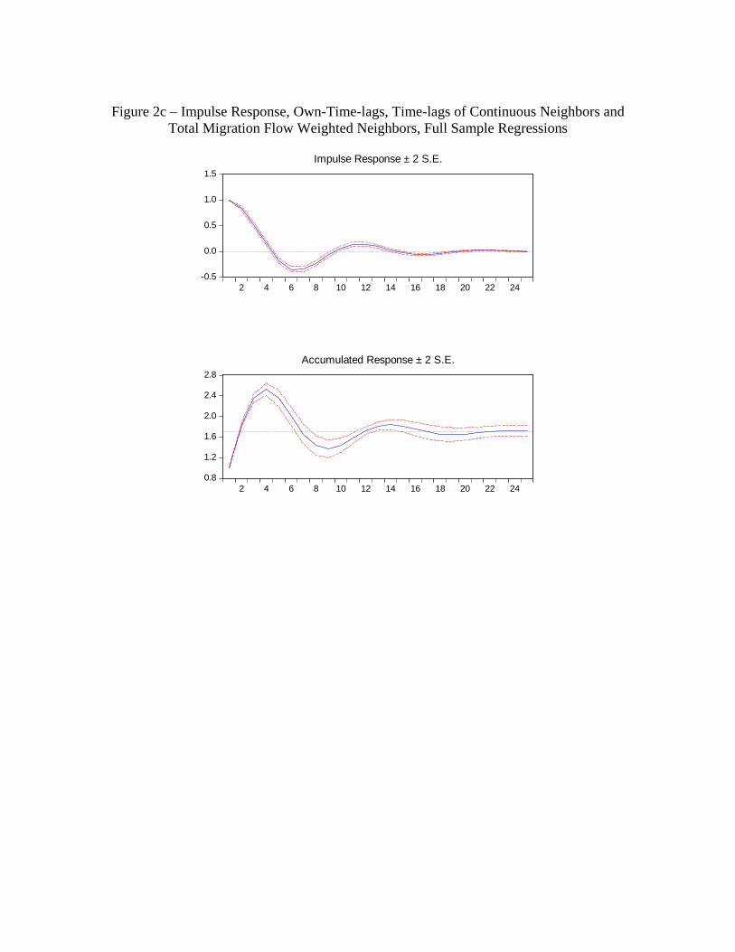
Figure 2c – Impulse Response, Own-Time-lags, Time-lags of Continuous Neighbors and

Total Migration Flow Weighted Neighbors, Full Sample Regressions

-0.5

0.0

0.5

1.0

1.5

2 4 6 8 10 12 14 16 18 20 22 24


0.8

1.2

1.6

2.0

2.4

2.8

2 4 6 8 10 12 14 16 18 20 22 24


Figure 3a: Impulse Response, Own Time-lags only, Post-2007 Regressions

-0.4

0.0

0.4

0.8

1.2

2 4 6 8 10 12 14 16 18 20 22 24


0.4

0.6

0.8

1.0

1.2

1.4

2 4 6 8 10 12 14 16 18 20 22 24


Figure 3b: Impulse Response, Own-Time-lags and Time-lags of Contiguous Neighbors, Post-2007 Regressions

-0.4

0.0

0.4

0.8

1.2

2 4 6 8 10 12 14 16 18 20 22 24


0.8

1.2

1.6

2.0

2 4 6 8 10 12 14 16 18 20 22 24


Figure 3c: Impulse Response, Own-Time-lags, Time-lags of Continuous Neighbors and

Total Migration Flow Weighted Neighbors, Post-2007 Regressions

-0.5

0.0

0.5

1.0

1.5

2 4 6 8 10 12 14 16 18 20 22 24


0.5

1.0

1.5

2.0

2.5

2 4 6 8 10 12 14 16 18 20 22 24


Table 1: 363 MSA’s in the continental U.S. (2009 U.S. Census Delineations)

Abilene, TX Denver-Aurora-Broomfield, CO Lancaster, PA Akron, OH

Des Moines-West Des Moines, IA Lansing-East Lansing, MI Racine, WI

Albany, GA

Detroit-Warren-Livonia, MI Laredo, TX

Rapid City, SD Albany-Schenectady-Troy, NY Dothan, AL

Las Cruces, NM

Reading, PA

Albuquerque, NM

Dover, DE

Las Vegas-Paradise, NV

Redding, CA Alexandria, LA

Dubuque, IA

Lawrence, KS

Reno-Sparks, NV

Allentown-Bethlehem-Easton, PA-NJ Duluth, MN-WI

Lawton, OK

Richmond, VA Altoona, PA

Durham-Chapel Hill, NC

Lebanon, PA

Riverside-San Bernardino-Ontario, CA

Amarillo, TX

Eau Claire, WI

Lewiston, ID-WA

Roanoke, VA Ames, IA

El Centro, CA

Lewiston-Auburn, ME

Rochester, MN

Anderson, IN

El Paso, TX

Lexington-Fayette, KY

Rochester, NY Anderson, SC

Elizabethtown, KY

Lima, OH

Rockford, IL

Ann Arbor, MI

Elkhart-Goshen, IN

Lincoln, NE

Rocky Mount, NC Anniston-Oxford, AL

Elmira, NY

Little Rock-North Little Rock-Conway, AR Rome, GA

Appleton, WI

Erie, PA

Logan, UT-ID

Sacramento--Arden-Arcade--Roseville, CA Asheville, NC

Eugene-Springfield, OR

Longview, TX

Saginaw-Saginaw Township North, MI

Athens-Clarke County, GA Evansville, IN-KY

Longview, WA

Salem, OR Atlanta-Sandy Springs-Marietta, GA Fargo, ND-MN

Los Angeles-Long Beach-Santa Ana, CA Salinas, CA

Atlantic City-Hammonton, NJ Farmington, NM

Louisville-Jefferson County, KY-IN Salisbury, MD Auburn-Opelika, AL

Fayetteville, NC

Lubbock, TX

Salt Lake City, UT

Augusta-Richmond County, GA-SC Fayetteville-Springdale-Rogers, AR-MO Lynchburg, VA

San Angelo, TX Austin-Round Rock, TX

Flagstaff, AZ

Macon, GA

San Antonio, TX

Bakersfield, CA

Flint, MI

Madera-Chowchilla, CA

San Diego-Carlsbad-San Marcos, CA Baltimore-Towson, MD

Florence, SC

Madison, WI

San Francisco-Oakland-Fremont, CA

Bangor, ME

Florence-Muscle Shoals, AL Manchester-Nashua, NH

San Jose-Sunnyvale-Santa Clara, CA Barnstable Town, MA

Fond du Lac, WI

Manhattan, KS

San Luis Obispo-Paso Robles, CA

Baton Rouge, LA

Fort Collins-Loveland, CO Mankato-North Mankato, MN Sandusky, OH Battle Creek, MI

Fort Smith, AR-OK

Mansfield, OH

Santa Barbara-Santa Maria-Goleta, CA

Bay City, MI

Fort Walton Beach-Crestview-Destin, FL McAllen-Edinburg-Mission, TX Santa Cruz-Watsonville, CA Beaumont-Port Arthur, TX Fort Wayne, IN

Medford, OR

Santa Fe, NM

Bellingham, WA

Fresno, CA

Memphis, TN-MS-AR

Santa Rosa-Petaluma, CA Bend, OR

Gadsden, AL

Merced, CA

Savannah, GA

Billings, MT

Gainesville, FL

Miami-Fort Lauderdale-Pompano Beach, FL Scranton--Wilkes-Barre, PA Binghamton, NY

Gainesville, GA

Michigan City-La Porte, IN Seattle-Tacoma-Bellevue, WA

Birmingham-Hoover, AL

Glens Falls, NY

Midland, TX

Sebastian-Vero Beach, FL Bismarck, ND

Goldsboro, NC

Milwaukee-Waukesha-West Allis, WI Sheboygan, WI

Blacksburg-Christiansburg-Radford, VA Grand Forks, ND-MN

Minneapolis-St. Paul-Bloomington, MN-WI Sherman-Denison, TX Bloomington, IN

Grand Junction, CO

Missoula, MT

Shreveport-Bossier City, LA

Bloomington-Normal, IL

Grand Rapids-Wyoming, MI Mobile, AL

Sioux City, IA-NE-SD Boise City-Nampa, ID

Great Falls, MT

Modesto, CA

Sioux Falls, SD

Boston-Cambridge-Quincy, MA-NH Greeley, CO

Monroe, LA

South Bend-Mishawaka, IN-MI Boulder, CO

Green Bay, WI

Monroe, MI

Spartanburg, SC

Bowling Green, KY

Greensboro-High Point, NC Montgomery, AL

Spokane, WA Bradenton-Sarasota-Venice, FL Greenville, NC

Morgantown, WV

Springfield, IL

Bremerton-Silverdale, WA Greenville-Mauldin-Easley, SC Morristown, TN

Springfield, MA Bridgeport-Stamford-Norwalk, CT Gulfport-Biloxi, MS

Mount Vernon-Anacortes, WA Springfield, MO

Brownsville-Harlingen, TX Hagerstown-Martinsburg, MD-WV Muncie, IN

Springfield, OH Brunswick, GA

Hanford-Corcoran, CA

Muskegon-Norton Shores, MI St. Cloud, MN

Buffalo-Niagara Falls, NY Harrisburg-Carlisle, PA

Myrtle Beach-North Myrtle Beach-Conway, SC St. George, UT Burlington, NC

Harrisonburg, VA

Napa, CA

St. Joseph, MO-KS

Burlington-South Burlington, VT Hartford-West Hartford-East Hartford, CT Naples-Marco Island, FL

St. Louis, MO-IL Canton-Massillon, OH

Hattiesburg, MS

Nashville-Davidson--Murfreesboro--Franklin, TN State College, PA

Cape Coral-Fort Myers, FL Hickory-Lenoir-Morganton, NC New Haven-Milford, CT

Stockton, CA Cape Girardeau-Jackson, MO-IL Hinesville-Fort Stewart, GA New Orleans-Metairie-Kenner, LA Sumter, SC Carson City, NV

Holland-Grand Haven, MI New York-Northern New Jersey-Long Island, NY-NJ-PA Syracuse, NY

Casper, WY

Hot Springs, AR

Niles-Benton Harbor, MI

Tallahassee, FL Cedar Rapids, IA

Houma-Bayou Cane-Thibodaux, LA Norwich-New London, CT Tampa-St. Petersburg-Clearwater, FL

Champaign-Urbana, IL

Houston-Sugar Land-Baytown, TX Ocala, FL

Terre Haute, IN Charleston, WV

Huntington-Ashland, WV-KY-OH Ocean City, NJ

Texarkana, TX-Texarkana, AR

Charleston-North Charleston-Summerville, SC Huntsville, AL

Odessa, TX

Toledo, OH Charlotte-Gastonia-Concord, NC-SC Idaho Falls, ID

Ogden-Clearfield, UT

Topeka, KS

Charlottesville, VA

Indianapolis-Carmel, IN

Oklahoma City, OK

Trenton-Ewing, NJ Chattanooga, TN-GA

Iowa City, IA

Olympia, WA

Tucson, AZ

Cheyenne, WY

Ithaca, NY

Omaha-Council Bluffs, NE-IA Tulsa, OK Chicago-Naperville-Joliet, IL-IN-WI Jackson, MI

Orlando-Kissimmee, FL

Tuscaloosa, AL

Chico, CA

Jackson, MS

Oshkosh-Neenah, WI

Tyler, TX Cincinnati-Middletown, OH-KY-IN Jackson, TN

Owensboro, KY

Utica-Rome, NY

Clarksville, TN-KY

Jacksonville, FL

Oxnard-Thousand Oaks-Ventura, CA Valdosta, GA Cleveland, TN

Jacksonville, NC

Palm Bay-Melbourne-Titusville, FL Vallejo-Fairfield, CA

Cleveland-Elyria-Mentor, OH Janesville, WI

Palm Coast, FL

Victoria, TX Coeur d'Alene, ID

Jefferson City, MO

Panama City-Lynn Haven-Panama City Beach, FL Vineland-Millville-Bridgeton, NJ

College Station-Bryan, TX Johnson City, TN

Parkersburg-Marietta-Vienna, WV-OH Virginia Beach-Norfolk-Newport News, VA-NC Colorado Springs, CO

Johnstown, PA

Pascagoula, MS

Visalia-Porterville, CA

Columbia, MO

Jonesboro, AR

Pensacola-Ferry Pass-Brent, FL Waco, TX Columbia, SC

Joplin, MO

Peoria, IL

Warner Robins, GA

Columbus, GA-AL

Kalamazoo-Portage, MI

Philadelphia-Camden-Wilmington, PA-NJ-DE-MD Washington-Arlington-Alexandria, DC-VA-MD-WV Columbus, IN

Kankakee-Bradley, IL

Phoenix-Mesa-Scottsdale, AZ Waterloo-Cedar Falls, IA

Columbus, OH

Kansas City, MO-KS

Pine Bluff, AR

Wausau, WI Corpus Christi, TX

Kennewick-Pasco-Richland, WA Pittsburgh, PA

Weirton-Steubenville, WV-OH

Corvallis, OR

Killeen-Temple-Fort Hood, TX Pittsfield, MA

Wenatchee-East Wenatchee, WA Cumberland, MD-WV

Kingsport-Bristol-Bristol, TN-VA Pocatello, ID

Wheeling, WV-OH

Dallas-Fort Worth-Arlington, TX Kingston, NY

Port St. Lucie, FL

Wichita Falls, TX Dalton, GA

Knoxville, TN

Portland-South Portland-Biddeford, ME Wichita, KS

Danville, IL

Kokomo, IN

Portland-Vancouver-Beaverton, OR-WA Williamsport, PA Danville, VA

La Crosse, WI-MN

Poughkeepsie-Newburgh-Middletown, NY Wilmington, NC

Davenport-Moline-Rock Island, IA-IL Lafayette, IN

Prescott, AZ

Winchester, VA-WV Dayton, OH

Lafayette, LA

Providence-New Bedford-Fall River, RI-MA Winston-Salem, NC

Decatur, AL

Lake Charles, LA

Provo-Orem, UT

Worcester, MA Decatur, IL

Lake Havasu City-Kingman, AZ Pueblo, CO

Yakima, WA

Deltona-Daytona Beach-Ormond Beach, FL Lakeland-Winter Haven, FL Punta Gorda, FL

York-Hanover, PA

Youngstown-Warren-Boardman, OH-PA

Yuba City, CA

Yuma, AZ

Table 2: Descriptive Statistics, Year-Over-Year Housing Price Growth and Spatial Lags, 1996-2013

Table 3 - Full Sample, 1996-2013*, MSA Fixed Effects (FE), HAC consistent std errors

Dependent Variable: House Price Index Growth between year t and t-1, for MSA i

FE FE post-2007 FE FE post-2007 FE FE, post-2007

constant 0.001337 -0.09922 0.001428 -0.102672 0.002258 -0.104176

0.067945 -6.627418 0.141102 -7.085534 0.225425 -6.72806

Lagged Growth (t-1) 0.664548 0.084501 0.654179 0.098031 0.6436 -0.008955

18.075 3.878959 48.45978 4.236311 44.90283 -0.302542

Lagged Growth (t-2) 0.137151 0.134437 0.117916 0.045018 0.088253 -0.06233

3.45083 7.44445 7.437054 2.303653 5.194735 -2.405071

Lagged Growth (t-3) -0.2712 -0.223971 -0.279876 -0.169536 -0.279778 -0.079483

-9.952059 -12.11822 -17.82169 -8.654643 -16.53972 -3.554155

Lagged Growth (t-4) -0.110793 -0.289164 -0.087911 -0.328221 -0.056998 -0.426242

-4.281305 -16.78527 -6.285872 -18.50129 -3.906895 -21.39453

Spatial Lag Growth (t-1) 0.013824 -0.092147 -0.001834 -0.139438

0.80296 -3.224093 -0.081042 -3.364402

Spatial Lag Growth (t-2) 0.077745 0.262061 -0.018413 0.017818

3.725996 10.97481 -0.63989 0.456435

Spatial Lag Growth (t-3) 0.036482 -0.103675 0.023508 0.02102

1.723244 -4.256112 0.788195 0.614495

Spatial Lag Growth (t-4) -0.131844 0.01562 0.011832 -0.045569

-6.753995 0.686782 0.44643 -1.511414

Spatial Migration Growth (t-1) 0.022077 0.245658

0.789402 6.136838


5.157995 11.23098

Spatial Migration Growth (t-3) 0.02896 -0.152578

0.784019 -3.296313

Spatial Migration Growth (t-4) -0.303739 0.017718

-8.718272 0.428054

R-squared 0.502698 0.689281 0.509927 0.711546 0.520496 0.735662

Numbers in italics are t-statistics

*regressions using migration data cover the years 1996-2011

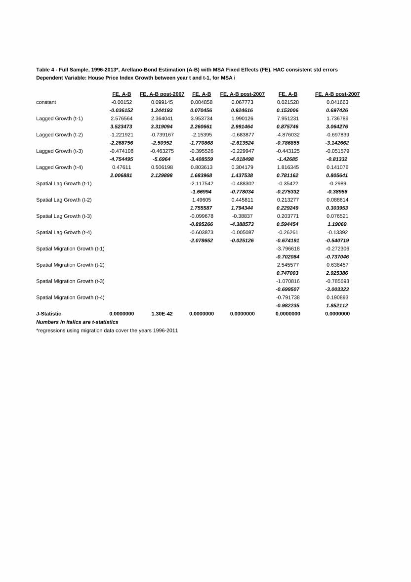
Table 4 - Full Sample, 1996-2013*, Arellano-Bond Estimation (A-B) with MSA Fixed Effects (FE), HAC consistent std errors


FE, A-B FE, A-B post-2007 FE, A-B FE, A-B post-2007 FE, A-B FE, A-B post-2007

constant -0.00152 0.099145 0.004858 0.067773 0.021528 0.041663

-0.036152 1.244193 0.070456 0.924616 0.153006 0.697426

Lagged Growth (t-1) 2.576564 2.364041 3.953734 1.990126 7.951231 1.736789

3.523473 3.319094 2.260661 2.991464 0.875746 3.064276

Lagged Growth (t-2) -1.221921 -0.739167 -2.15395 -0.683877 -4.876032 -0.697839

-2.268756 -2.50952 -1.770868 -2.613524 -0.786855 -3.142662

Lagged Growth (t-3) -0.474108 -0.463275 -0.395526 -0.229947 -0.443125 -0.051579

-4.754495 -5.6964 -3.408559 -4.018498 -1.42685 -0.81332

Lagged Growth (t-4) 0.47611 0.506198 0.803613 0.304179 1.816345 0.141076

2.006881 2.129898 1.683968 1.437538 0.781162 0.805641

Spatial Lag Growth (t-1) -2.117542 -0.488302 -0.35422 -0.2989

-1.66994 -0.778034 -0.275332 -0.38956

Spatial Lag Growth (t-2) 1.49605 0.445811 0.213277 0.088614

1.755587 1.794344 0.229249 0.303953

Spatial Lag Growth (t-3) -0.099678 -0.38837 0.203771 0.076521

-0.895266 -4.388573 0.594454 1.19069


-2.078652 -0.025126 -0.674191 -0.540719

Spatial Migration Growth (t-1) -3.796618 -0.272306

-0.702084 -0.737046


0.747003 2.925386


-0.699507 -3.003323


-0.982235 1.852112

J-Statistic 0.0000000 1.30E-42 0.0000000 0.0000000 0.0000000 0.0000000



Table 5 - Full Sample, 1996-2013*, HAC consistent standard errors


no FE no FE, post-2007 no FE no FE, post-2007 no FE no FE, post-2007

constant 0.00382 -0.021939 0.004607 -0.023936 0.0060640 -0.02122

3.487911 -11.64791 4.37067 -13.48862 6.010982 -12.93094512

Lagged Growth (t-1) 0.672533 0.478725 0.664584 0.540908 0.655723 0.602968

18.70821 10.82139 17.67518 11.85372 16.12177 11.51922068

Lagged Growth (t-2) 0.136279 0.122189 0.117397 0.034178 0.089001 -0.05131

3.556629 2.747557 3.059331 0.717341 2.131005 -0.927563456

Lagged Growth (t-3) -0.270765 -0.307033 -0.278418 -0.231338 -0.277587 -0.1602

-10.26015 -10.63542 -9.8116 -6.937455 -8.964133 -4.201234687

Lagged Growth (t-4) -0.100301 -0.133555 0.076787 -0.145981 -0.044938 -0.158747

-4.012427 -4.768795 3.090475 -5.590306 -1.746022 -6.021921589

Spatial Lag Growth (t-1) 0.008156 -0.242515 -0.004862 -0.121056

0.376996 -7.707917 -0.196076 -3.972923108

Spatial Lag Growth (t-2) 0.07703 0.259168 -0.015511 0.062557

2.703624 7.022555 -0.486195 1.640124166

Spatial Lag Growth (t-3) 0.034513 -0.131958 0.023463 0.035289

1.295186 -3.702765 0.842933 0.979088223

Spatial Lag Growth (t-4) -0.134064 -0.049341 0.009566 -0.058565

-5.431445 -1.879395 0.365081 -2.187505119


0.430273 -3.929054637


3.393715 5.811981821


0.564772 -4.980840253


-6.189478 -0.437442712

R-squared 0.497454 0.516028 0.504427 0.542619 0.514814 0.558572



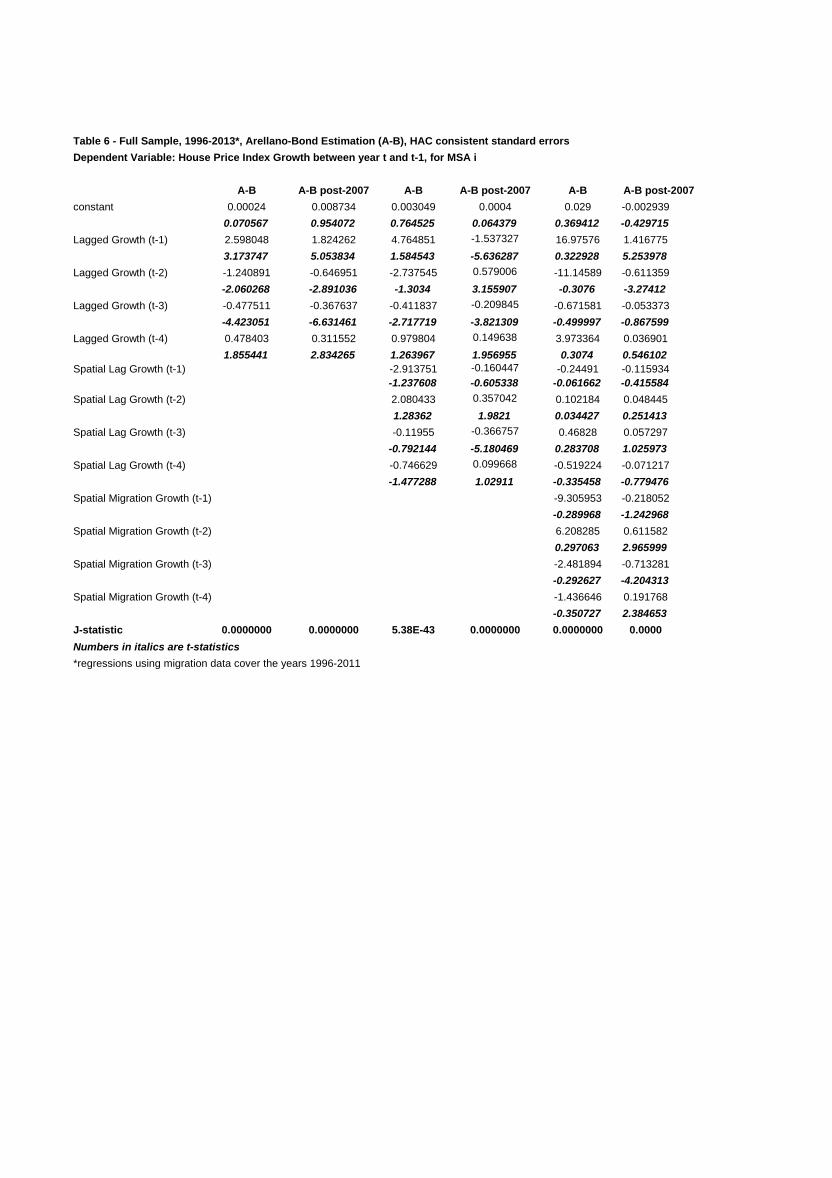
Table 6 - Full Sample, 1996-2013*, Arellano-Bond Estimation (A-B), HAC consistent standard errors


A-B A-B post-2007 A-B A-B post-2007 A-B

constant 0.00024 0.008734 0.003049 0.0004 0.029 -0.002939

0.070567 0.954072 0.764525 0.064379 0.369412 -0.429715

Lagged Growth (t-1) 2.598048 1.824262 4.764851 -1.537327 16.97576 1.416775

3.173747 5.053834 1.584543 -5.636287 0.322928 5.253978

Lagged Growth (t-2) -1.240891 -0.646951 -2.737545 0.579006 -11.14589 -0.611359

-2.060268 -2.891036 -1.3034 3.155907 -0.3076 -3.27412

Lagged Growth (t-3) -0.477511 -0.367637 -0.411837 -0.209845 -0.671581 -0.053373

-4.423051 -6.631461 -2.717719 -3.821309 -0.499997 -0.867599

Lagged Growth (t-4) 0.478403 0.311552 0.979804 0.149638 3.973364 0.036901

1.855441 2.834265 1.263967 1.956955 0.3074 0.546102


-1.237608 -0.605338 -0.061662 -0.415584

Spatial Lag Growth (t-2) 2.080433 0.357042 0.102184 0.048445

1.28362 1.9821 0.034427 0.251413

Spatial Lag Growth (t-3) -0.11955 -0.366757 0.46828 0.057297

-0.792144 -5.180469 0.283708 1.025973

Spatial Lag Growth (t-4) -0.746629 0.099668 -0.519224 -0.071217

-1.477288 1.02911 -0.335458 -0.779476


-0.289968 -1.242968


0.297063 2.965999


-0.292627 -4.204313


-0.350727 2.384653

J-statistic 0.0000000 0.0000000 5.38E-43 0.0000000 0.0000000 0.0000



A-B post-2007

Documents

Spatial Effects and House Price Dynamics in the U.S.A. · PDF fileSpatial Effects and House Price Dynamics ... submarket within an MSA and the return at ... diffusion patterns exist