Spatial distribution of glacial erosion rates in the St. Elias

Spatial distribution of glacial erosion rates in the St. Elias range,Alaska, inferred from a realistic model of glacier dynamics

Rachel Headley,1,2 Bernard Hallet,1 Gerard Roe,1 Edwin D. Waddington,1 and Eric Rignot3,4

Received 29 November 2011; revised 29 June 2012; accepted 11 July 2012; published 8 September 2012.

[1] Glaciers have been principal erosional agents in many orogens throughout much of therecent geological past. A modern example is the St. Elias Mountains in southeasternAlaska; it is a highly convergent, complex orogen, which has been glaciated for much of itshistory. We examine the Seward-Malaspina Glacier system, which comprises two of thelargest temperate glaciers in the world. We focus on the pattern of erosion within its narrowpassage through the St. Elias Mountains, the Seward Throat. Measured glacier surfacevelocities and elevations provide constraints for a full-stress numerical flowband modelthat enables us to quantitatively determine the glacier thickness profile, which is not easilymeasured on temperate glaciers, and the basal characteristics relevant for erosion. Thesecharacteristics at the bed, namely the water pressure, normal and shear stresses, and slidingvelocity, are then used to infer the spatial variation in erosion rates using several commonlyinvoked erosion laws. The calculations show that the geometry of the glacier basin exerts afar stronger control on the spatial variation of erosion rates than does the equilibrium linealtitude, which is often assumed to be important in studies of glaciated orogens. The modelprovides a quantitative basis for understanding why erosion rates are highest around theSeward Throat, which is generally consistent with local and large-scale geologicalobservations and thermochronologic evidence. Moreover, model results suggest howglacier characteristics could be used to infer zones of active or recent uplift in ice-mantledorogens.

Citation: Headley, R., B. Hallet, G. Roe, E. D. Waddington, and E. Rignot (2012), Spatial distribution of glacial erosion rates inthe St. Elias range, Alaska, inferred from a realistic model of glacier dynamics, J. Geophys. Res., 117, F03027,doi:10.1029/2011JF002291.

1. Introduction

[2] The interactions among surface processes, climate, andtectonics in active orogens have been at the forefront ofEarth science research in recent decades [e.g., Molnar andEngland, 1990; Beaumont et al., 1992; Koons, 1995;Zeitler et al., 2001; Wobus et al., 2003; Bookhagen et al.,2005]. There is considerable interest in glacial erosion intectonically active mountain ranges [e.g., Tomkin and

Braun, 2002; Herman and Braun, 2008; Yanites andEhlers, 2012] because erosion by temperate glaciers, espe-cially those in Alaska, can be exceptionally fast and tends tobe an important or dominant exhumation agent in activeorogens through the Quaternary [Hallet, 1996; Delmas et al.,2009; Koppes and Montgomery, 2009]. While modeling therole of glaciers in orogenic development has yielded usefulinsights [Tomkin, 2007; Herman and Braun, 2008], much isto be learned from glaciologically focused studies of cur-rently glaciated, tectonically active regions.[3] The St. Elias Mountains constitute a prime example of

an active, compressional orogen being impacted by climate,through the erosion by the large glaciers in the region [e.g.,Meigs and Sauber, 2000; Spotila et al., 2004]. The large-scale patterns (both temporal and spatial) of tectonic devel-opment, exhumation, and sedimentation have been identi-fied through diverse studies of the structural geology,thermochronology, and offshore geophysics [Jaeger et al.,1998; Bruhn et al., 2004; Berger et al., 2008; Chapmanet al., 2008; Enkelmann et al., 2010]. Across the glaciersin southern Alaska, recent basin-averaged erosion rates havebeen estimated from glacier sediment output [Humphrey andRaymond, 1994; Hallet, 1996; Koppes and Hallet, 2006] and

1Department of Earth and Space Sciences, University of Washington,Seattle, Washington, USA.

2Now at Institut für Geowissenschaften, Universität Tübingen,Tübingen, Germany.

3Department of Earth System Science, University of California, Irvine,California, USA.

4Jet Propulsion Laboratory, California Institute of Technology,Pasadena, California, USA.

Corresponding author: R. Headley, Institut für Geowissenschaften,Universität Tübingen, Wilhelmstrasse 56, D-72074 Tübingen, Germany.([email protected])

©2012. American Geophysical Union. All Rights Reserved.0148-0227/12/2011JF002291

JOURNAL OF GEOPHYSICAL RESEARCH, VOL. 117, F03027, doi:10.1029/2011JF002291, 2012

F03027 1 of 16

offshore sediment volumes [Jaeger et al., 1998; Sheaf et al.,2003]. While large-scale exhumation patterns and basin-averaged erosion rates are informative of the dynamics of theorogen, details of how the erosion rate varies over thelandscape requires a closer look at specific glaciers.[4] We consider an exceptionally fast-moving portion of

one the region’s principal glacier systems, the SewardThroat of the Seward-Malaspina system. This work capita-lizes on empirical data available for this glacier and uses a2D full-stress numerical model of glacier flow to define thespatial variability of the ice thickness and basal character-istics. While we focus on a specific glacier, the methodcould be used on any glacier for which sufficient data existto constrain the model. For many temperate glaciers, the icethickness and basal properties are not easily measured. Overthe Seward Throat, airborne radar measurements of glacierthickness have been largely unsuccessful because the glacieris thick and heavily crevassed. We start off by determiningthe ice thickness using the numerical model constrained byobserved surface velocities and elevations. We then calcu-late the basal characteristics relevant for erosion, includingthe sliding velocity, water pressure, and normal and shearstresses. From these properties, we infer the spatial variationin erosion rates and discuss it in the context of empirical data

defining the spatial variation of rates of exhumation andcrustal deformation in the region.

2. Setting

2.1. Glaciological Setting

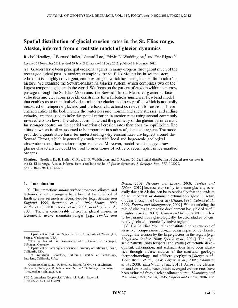
[5] The Seward-Malaspina Glacier system is in southeast-ern coastal Alaska and extends into the southwestern cornerof the Yukon Territory in Canada, east of Mt. St. Elias(Figure 1). It covers around 3900 km2 and originates in theSaint Elias Mountains and on the Mount Logan massif,where peaks exceed 5500 m above sea level and precipitationis high. The nearest long-term meteorological measurementsare from Yakutat, a coastal town around 40 km to the SE andacross Yakutat Bay; the annual precipitation and temperatureaverage 5 m and 4�C, respectively (http://www.wrcc.dri.edu/summary/yak.ak.html; accessed November 2008). From theSeward Ice Field, which is an accumulation area exceeding60 km in width, the ice funnels through the mountains in a 4–6 km wide passage, which drops steeply from approximately1500 m to 600 m above sea level (Figure 1). This narrowpassage, the Seward Throat, is the focus of this paper. Southof the Seward Throat, the glacier spreads out in a largepiedmont lobe, forming the main portion of Malaspina

Figure 1. Entire Seward-Malaspina glacier system; inset shows location in Alaska. The Seward Throat isoutlined in red. The major faults are labeled in italics, including the principal thrust faults, the Chugach St.Elias fault and the Malaspina fault [Enkelmann et al., 2008].

HEADLEY ET AL.: SEWARD THROAT GLACIAL EROSION RATES F03027F03027

2 of 16

Glacier. This lobe is also fed from the west by Agassiz Gla-cier and from the east by several smaller glaciers. The dis-tinctive piedmont lobe of Malaspina Glacier has beenextensively investigated [e.g., Sharp, 1951; Allen and Smith,1953; Ford et al., 2003], while the Seward Throat hasreceived considerably less attention due largely to the rug-gedness and inaccessibility of the terrain.[6] Glacial coverage has been continuous in the St. Elias

Mountains from the Pliocene to the present [Péwé, 1975].Offshore sediments indicate that Malaspina Glacier waslikely a tidewater glacier that extended perhaps 100 km ontothe continental shelf at the Last Glacial Maximum [Molnia,1986; W. F. Manley and D. S. Kaufman, Alaska PaleoGla-cier Atlas: Institute of Arctic and Alpine Research: AGeospatial Compilation of Pleistocene Glacier Extents,2002, http://instaar.colorado.edu/QGISL/ak_paleoglacier_atlas/, hereinafter referred to as Manley and Kaufman, onlinedata, 2002]. While there is currently little or no calving, forthe last century Malaspina Glacier has terminated at or nearthe Pacific coast [Porter, 1989].[7] This region is one of few where orogen-scale and

basin-averaged glacial erosion rates have been extensivelystudied. Averaged over the length of the entire St. Eliasrange, offshore sedimentation rates imply erosion rates of5.1 mm yr�1 for the past 104 years [Sheaf et al., 2003] andsimilar rates for the last century [Jaeger et al., 1998]. Thebasin-wide erosion rate has been estimated for glaciersadjacent to, and within similar climatic and structural set-tings as, the Seward-Malaspina system. This rate averagesover 9 mm yr�1 for Tyndall Glacier in Icy Bay over the lastcenturies [Koppes and Hallet, 2006] and around 11 mm yr�1

for Hubbard Glacier [Trusel et al., 2008].

2.2. Geological Setting

[8] This region’s glaciological and geological histories aretightly intertwined, with evidence (particularly ice-rafteddebris in the Pacific) of syn-collisional glacier cover anderosion starting as early as 5.6Ma [Plafker, 1987; Lagoe et al.,1993; Plafker et al., 1994]. The tectonic setting of the Seward-Malaspina system has been dominated by convergencebetween the Yakutat terrane and North America since 5–10 Ma [Plafker et al., 1994; Meigs et al., 2008]. Many majorfaults traverse this region, including the Chugach St. Eliasthrust fault and Contact Fault, which is completely underglacial cover (Figure 1) but can be been inferred from geodeticmeasurements, structural analysis of the surrounding region,and geological observations on isolated nunataks [e.g., Bruhnet al., 2004; Chapman et al., 2008; Elliott et al., 2010]. TheSeward and Malaspina glaciers cover many of these majorfaults and associated ancillary structures, both active andinactive (Figure 1).[9] Currently, geodetic studies show overall NW-SE

crustal convergence between the Yakutat Block and south-ern Alaska; 37 mm yr�1 of convergence occurs mainlybetween the coast and the Bagley and Seward Ice Fields, adistance of around 70 km [Elliott et al., 2010; Elliott, 2011].For comparison, the corresponding strain rate, assuming aconservative estimate of 20 mm yr�1 across the 70 km dis-tance, is slightly higher than that occurring in the Himalaya,which is 15�20 mm yr–1 [Zhang et al., 2004] over a dis-tance of about 100 km. Seismic studies of the St. Elias rangeare consistent with geodetic observations and also highlight

a region of enhanced activity situated between the coast andice fields [Pavlis et al., 2008]. Thus, the Seward Throat cutsacross a zone of exceptionally active crustal convergence,where rapid and variable rock uplift is expected and isreflected in the extreme topography, including Mt. St. Elias,the third highest peak in North America.

2.3. Data Coverage

[10] Over the past decade, satellite and airborne instru-ments have provided invaluable surface-elevation, thickness,and velocity measurements for many ice masses, includingthe Seward-Malaspina system. Here we use high-resolutiondigital elevation models (DEMs) of the ice and surroundingregion derived from the Shuttle Radar Topography Mission(SRTM) measurements; they were acquired during winter2000, at 30 m resolution over most of the glacier system,with vertical accuracy of about 16 m [Muskett et al., 2008].Part of the accumulation area lies above 60.5�N, where thereis no SRTM coverage, but this portion is not considered inthis work. While the surface elevation of Malaspina Glaciercan change rapidly from both surging [Muskett et al., 2008]and mass loss due to a warming climate [Sauber et al.,2005], the ice surface through the Seward Throat appearsto have lowered fairly uniformly by less than a few meterssince 2000 based on comparisons of the SRTM measure-ments with more recent airborne laser profiles [Arendt et al.,2008].[11] Compared to the elevation of the ice surface, the

glacier thickness in the study region is essentially unknown.Conway et al. [2009] conducted an airborne ice-penetratingradar survey, in 2005, to determine glacier thicknesses in theregion. The measurements were successful over sections ofMalaspina Glacier but not through the Seward Throat, likelydue to severe surface crevassing [Conway et al., 2009].However, these measurements still provide important con-straints for determining the ice thickness, as describedbelow. Uncertainties for these ice thickness measurementsare small, generally less than 18 m [Conway et al., 2009].[12] In contrast to the ice thickness, high-resolution sur-

face velocity measurements are available and are presentedin Figure 2. The data used to generate this velocity map(Figure 2) were acquired by the Canadian Space Agency’sRADARSAT-1 synthetic aperture radar, which operates atC-band frequency (5.6 GHz), with horizontal transmit andreceive polarization. We combined orbits 25333 and 25676acquired in fine beam mode F1 on, respectively, 9/11/2000and 10/5/2000, i.e., 24 days apart. The data were processedusing a speckle tracking algorithm [Michel and Rignot,1999] and assuming surface parallel flow to obtain a three-dimensional vector of ice flow. The data effectively repre-sent the average speed of the ice over a 24-day period.SRTM is used for topographic control. The pixel spacing ofthe radar data is 7.5 m on the ground in the radar-lookingdirection, and 6.1 m in the along track direction. Measure-ment noise is nominally about 1/100th of a pixel, which isequivalent to approximately 1 m yr�1. In practice, thevelocity measurements have a precision of a few meters peryear, which is small compared to the speed of the glacier(1 km yr�1). Good measurements are obtained in the SewardThroat. Data quality degrades on the Malaspina lobe due torapid surface melting, and in the upper reaches of the glacierdue to surface weathering and lower signal-to-noise ratio.


3 of 16

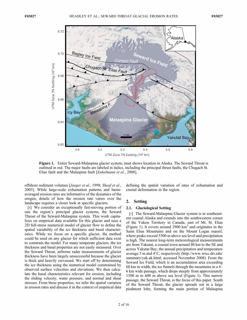
[13] As ice funnels from the Seward Ice Field through theSeward Throat, surface velocities increase, over tens ofkilometers, from less than 0.5 km yr�1 to over 1.8 km yr�1

(Figure 2). Point measurements of surface velocity in the

lower section of the Seward Throat made by Austin Post inthe summer of 1971 (unpublished) and by Headley et al.[2007] in the summer of 2007 are similar, suggesting thatthe overall spatial pattern of surface velocity is stable over atleast a few decades. Because mass balance has little

Figure 2. (a) The Seward Throat surface velocities and flow vectors (section 2.3). The maximum veloc-ities approach 2 km yr�1. The flowband, defined by the flow vectors, used in the analysis is highlighted inwhite. Ice thickness was measured at the pink star. (b) Surface profile (black line) and bed profiles (blueand red lines), with no vertical exaggeration. Red line is the initial bed found from simple mass conserva-tion (equation (1)) and shallow-ice approximations; the blue line is the best fit bed using the full-stressmodel constrained by measured surface topography and velocity. Red vertical bars correspond to thered flowband gates in Figure 2a. (c) Measured surface velocity in black (left axis; dashed where observa-tions were missing and have been interpolated). The standard deviation of the mean velocity is less than10% over the profile. Range of seasonal and inter-annual variation over a few years is shown in light graybased on Burgess et al. [2010]. Flowband widths are shown in green (right axis). In the 5-to-10 km reachnear the entrance of the Throat, where insufficient velocity data exist to constrain the width, three interpo-lations are shown: the flowband shown in Figure 4a (long-dashes), spline fit between 6 and 11 km (short-dashes), and a spline fit between 3 and 11 km (dots).


4 of 16

influence on flow through the Seward Throat, as discussedin Section 3.1, surface elevation is controlled primarily bythe ice flux entering from the ice field above. Using thisassumption, to transit the 40 km length of the Seward Throatat an average speed of 1 km yr�1 takes about 40 years, whichcan be interpreted as a characteristic time to change thesurface elevation. Since observations are available from over40 years ago, we determine that large but slow thicknesschanges are not ongoing. Although the overall pattern isfairly robust, annual and seasonal variations in speed dooccur. Burgess et al. [2010] found such variations in thesurface velocity, with the largest variation near the surfacevelocity peaks around down-glacier distances 20 km and27–31 km (Figure 2c). Temporal changes in subglacialhydrology are the most likely causes for these velocity var-iations [e.g., Gordon et al., 1998; Harper et al., 2005]. Thesensitivity of the modeled basal sliding to the basal waterpressure is explored in Section 3.4. Despite these variations,however, the overall observed spatial distribution of velocityis robust and provides a sound empirical basis for definingthe bed by estimating ice thickness.

3. Determining the Bed Topography

[14] The glacier thickness is addressed along a two-dimensional section (Figure 2) defined by a flowbandextending down the center of the Seward Throat. To mini-mize sidewall effects and define a region of conserved iceflow, the boundaries of this flowband (Figure 2a) areinferred from flow lines defined by the InSAR surfacevelocity vectors, which are interpolated on a 50 m by 50 mgrid. In order to minimize the effects of uncertainty in anygiven vector, the minimum width of the flowband has beenchosen to be around an order of magnitude larger than thisgrid spacing. This width ranges from about 0.3 to 1.4 km(Figure 2c). Because the velocities in the reach between 6and 11 km are poorly defined, uncertainties in the width ofthe flow band in this region are significantly larger than forthe rest of the Seward Throat; the width through this reach isinferred using a smooth function to interpolate the velocities(Figure 2c shows three possibilities). For the remainder ofthe analysis, we use the velocity, and elevations of the icesurface and of the bed averaged across this single, centralflowband (Figures 2b and 2c).[15] In order to find the ice thickness, the following steps

are undertaken: Initial estimates for the glacier thickness arefound using a simple mass conservation method. The bedfrom this method is then evaluated within a 2D full-stressglacier flow line model, and considerable discrepanciesbetween observed and modeled surface velocities are foundover a large section of the Seward Throat. Finally, we refinethe calculated bed elevation to provide a closer matchbetween measured surface velocities and values modeledusing the full stress model.

3.1. Initial Thickness Estimate

[16] For other large Alaskan glaciers, a mass conservationmethod based upon the shallow ice approximation (SIA) hasbeen used to find the ice thickness [e.g., Rasmussen, 1989;O’Neel et al., 2005]. The SIA neglects the effects of thelongitudinal stresses relative to the shear stresses, so that ice

motion is dependent only upon local topographic effects[Paterson, 1994], and the mass conservation methodassumes that the ice flux and the surface velocity are definedat all points along the glacier. The ice flux is the product ofice thickness H, the flow-band width, W, and ū, the depth-averaged velocity, which can be related to the surfacevelocity (usurf) by ū = a usurf. The flux is thus defined byF = a usurf HW. For the shallow ice approximation, a with avalue of 0.8 represents only deformation with no sliding, anda with a value of 1.0 is all sliding. Empirical values of a of0.8 or more are not uncommon for fast-moving, temperateglaciers [Paterson, 1994, p. 135].[17] For the Seward Throat, the flux can be defined where

x0 = 36 km along the glacier length (Figure 2), where radarmeasurements [Conway et al., 2009] define the ice thick-ness: H(x0) = 800 m. Following O’Neel et al. [2005], weassume that a does not vary spatially in this initial estimateof the thickness, so that a cancels out when comparing theflux between any two locations. With the additionalassumption that the flux is spatially uniform, the thickness asa function of distance downglacier can be estimated from:

H xð Þ ¼ H x0ð ÞW x0ð Þusurf x0ð ÞW xð Þusurf xð Þ ; ð1Þ

where usurf (x) is based on the satellite radar measurementsand W(x) is determined from the local width of the chosenflowband (Figures 2a and 2c). The small effect of ice lossdue to ablation on the ice flux through this short reach isneglected in this calculation, though it could be readilyincorporated [e.g., O’Neel et al., 2005]. Mass balanceobservations in the region are sparse [Sharp, 1951;Meier andPost, 1962; Tangborn, 1999]. Assuming a liberal 2 m yr�1 ofablation over the 40 km length of the Seward Throat, themass balance accounts for a loss of 8� 104 m2 yr�1 averagedover the width, compared to a conservative width-averagedaverage flux of 8 � 105 m2 yr�1 from 800 m thick icemoving at 1 km yr�1. From this calculation, ablational lossthrough the Seward Throat is around 10% of the ice flux andis thus considered negligible in this context.[18] Using equation (1), we calculate the ice thickness

along the flowband at uniform distance increments of 200 m.The 18 m uncertainty in the thickness measurement has anegligible (less than 2%) effect on the calculated thicknessprofile. We solve for thickness at each point locally usingequation (1), so that transient effects or errors in the surfacetopography directly translate to the bed. In order to focusonly on the broader features of the topography under the ice,the resulting bed profile is smoothed using a first-orderButterworth filter, which maintains locations of major fea-tures and the general shape of the bed but filters out higher-frequency roughness. The averaging length-scale of thisfilter is comparable to the typical longitudinal-coupling scaleof 4–5 ice thicknesses for valley glaciers [Echelmeyer andKamb, 1986; Kamb and Echelmeyer, 1986]. In the result-ing bed profile (Figure 2b), the ice thicknesses are compa-rable to those of similar glaciers in Alaska, such as thosederived from airborne ice-penetrating radar on the adjacentBering glacier [Conway et al., 2009] and bathymetric mea-surements in the bay formerly covered by Columbia Glacier[O’Neel et al., 2005].


5 of 16

3.2. Evaluation and Improvementof the Thickness Estimate

[19] To refine the ice thickness estimate, as well as todefine the basal properties relevant for erosion, a full-stressflowband model has been developed using the commercial,finite element software package COMSOL Multiphysics®.The basic model uses the plane strain momentum equationsfor nonlinear, temperate ice, based on the work of Johnsonand Staiger [2007] and Campbell [2009]. While concernshave been raised about the model of Johnson and Staiger[2007], specifically of how their model generates velocitiesthat are low over steep, shallow reaches [Kavanaugh et al.,2009; Golledge and Levy, 2011], the incorporation ofwidth variations following Pattyn [2002] and sliding(equation (A12)) within our model directly addresses manyof these issues. The model is described in detail in AppendixA and parameters are given in Table 1.[20] Using the initial thickness profile described in

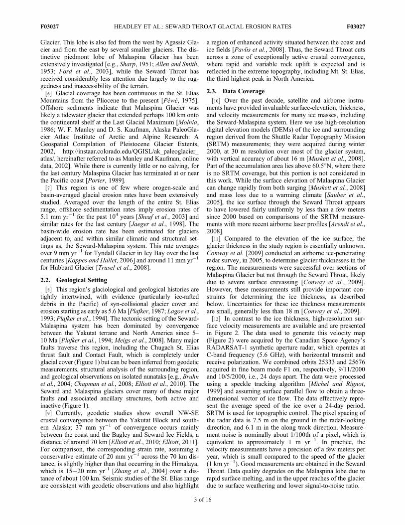
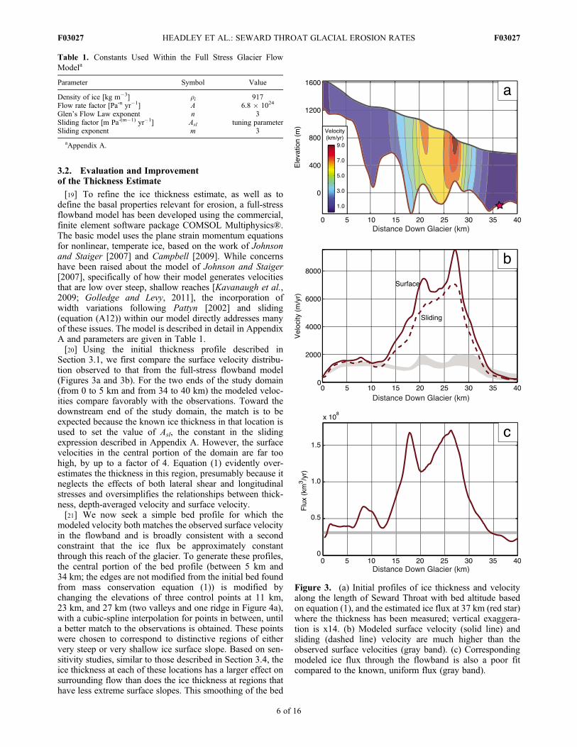
Section 3.1, we first compare the surface velocity distribu-tion observed to that from the full-stress flowband model(Figures 3a and 3b). For the two ends of the study domain(from 0 to 5 km and from 34 to 40 km) the modeled veloc-ities compare favorably with the observations. Toward thedownstream end of the study domain, the match is to beexpected because the known ice thickness in that location isused to set the value of Asl, the constant in the slidingexpression described in Appendix A. However, the surfacevelocities in the central portion of the domain are far toohigh, by up to a factor of 4. Equation (1) evidently over-estimates the thickness in this region, presumably because itneglects the effects of both lateral shear and longitudinalstresses and oversimplifies the relationships between thick-ness, depth-averaged velocity and surface velocity.[21] We now seek a simple bed profile for which the

modeled velocity both matches the observed surface velocityin the flowband and is broadly consistent with a secondconstraint that the ice flux be approximately constantthrough this reach of the glacier. To generate these profiles,the central portion of the bed profile (between 5 km and34 km; the edges are not modified from the initial bed foundfrom mass conservation equation (1)) is modified bychanging the elevations of three control points at 11 km,23 km, and 27 km (two valleys and one ridge in Figure 4a),with a cubic-spline interpolation for points in between, untila better match to the observations is obtained. These pointswere chosen to correspond to distinctive regions of eithervery steep or very shallow ice surface slope. Based on sen-sitivity studies, similar to those described in Section 3.4, theice thickness at each of these locations has a larger effect onsurrounding flow than does the ice thickness at regions thathave less extreme surface slopes. This smoothing of the bed

Table 1. Constants Used Within the Full Stress Glacier FlowModela

Parameter Symbol Value

Density of ice [kg m�3] ri 917Flow rate factor [Pa-n yr�1] A 6.8 � 1024

Glen’s Flow Law exponent n 3Sliding factor [m Pa-(m�1) yr�1] Asl tuning parameterSliding exponent m 3

aAppendix A.

Figure 3. (a) Initial profiles of ice thickness and velocityalong the length of Seward Throat with bed altitude basedon equation (1), and the estimated ice flux at 37 km (red star)where the thickness has been measured; vertical exaggera-tion is x14. (b) Modeled surface velocity (solid line) andsliding (dashed line) velocity are much higher than theobserved surface velocities (gray band). (c) Correspondingmodeled ice flux through the flowband is also a poor fitcompared to the known, uniform flux (gray band).


6 of 16

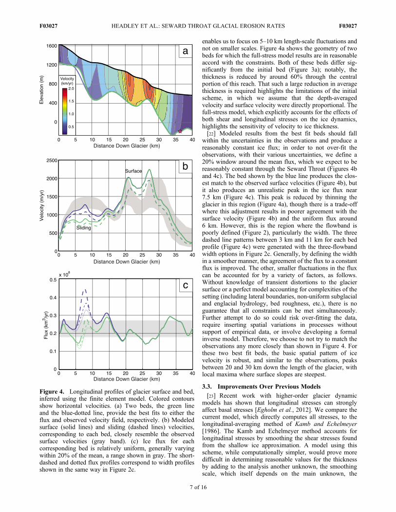
enables us to focus on 5–10 km length-scale fluctuations andnot on smaller scales. Figure 4a shows the geometry of twobeds for which the full-stress model results are in reasonableaccord with the constraints. Both of these beds differ sig-nificantly from the initial bed (Figure 3a); notably, thethickness is reduced by around 60% through the centralportion of this reach. That such a large reduction in averagethickness is required highlights the limitations of the initialscheme, in which we assume that the depth-averagedvelocity and surface velocity were directly proportional. Thefull-stress model, which explicitly accounts for the effects ofboth shear and longitudinal stresses on the ice dynamics,highlights the sensitivity of velocity to ice thickness.[22] Modeled results from the best fit beds should fall

within the uncertainties in the observations and produce areasonably constant ice flux; in order to not over-fit theobservations, with their various uncertainties, we define a20% window around the mean flux, which we expect to bereasonably constant through the Seward Throat (Figures 4band 4c). The bed shown by the blue line produces the clos-est match to the observed surface velocities (Figure 4b), butit also produces an unrealistic peak in the ice flux near7.5 km (Figure 4c). This peak is reduced by thinning theglacier in this region (Figure 4a), though there is a trade-offwhere this adjustment results in poorer agreement with thesurface velocity (Figure 4b) and the uniform flux around6 km. However, this is the region where the flowband ispoorly defined (Figure 2), particularly the width. The threedashed line patterns between 3 km and 11 km for each bedprofile (Figure 4c) were generated with the three-flowbandwidth options in Figure 2c. Generally, by defining the widthin a smoother manner, the agreement of the flux to a constantflux is improved. The other, smaller fluctuations in the fluxcan be accounted for by a variety of factors, as follows.Without knowledge of transient distortions to the glaciersurface or a perfect model accounting for complexities of thesetting (including lateral boundaries, non-uniform subglacialand englacial hydrology, bed roughness, etc.), there is noguarantee that all constraints can be met simultaneously.Further attempt to do so could risk over-fitting the data,require inserting spatial variations in processes withoutsupport of empirical data, or involve developing a formalinverse model. Therefore, we choose to not try to match theobservations any more closely than shown in Figure 4. Forthese two best fit beds, the basic spatial pattern of icevelocity is robust, and similar to the observations, peaksbetween 20 and 30 km down the length of the glacier, withlocal maxima where surface slopes are steepest.

3.3. Improvements Over Previous Models

[23] Recent work with higher-order glacier dynamicmodels has shown that longitudinal stresses can stronglyaffect basal stresses [Egholm et al., 2012]. We compare thecurrent model, which directly computes all stresses, to thelongitudinal-averaging method of Kamb and Echelmeyer[1986]. The Kamb and Echelmeyer method accounts forlongitudinal stresses by smoothing the shear stresses foundfrom the shallow ice approximation. A model using thisscheme, while computationally simpler, would prove moredifficult in determining reasonable values for the thicknessby adding to the analysis another unknown, the smoothingscale, which itself depends on the main unknown, the

Figure 4. Longitudinal profiles of glacier surface and bed,inferred using the finite element model. Colored contoursshow horizontal velocities. (a) Two beds, the green lineand the blue-dotted line, provide the best fits to either theflux and observed velocity field, respectively. (b) Modeledsurface (solid lines) and sliding (dashed lines) velocities,corresponding to each bed, closely resemble the observedsurface velocities (gray band). (c) Ice flux for eachcorresponding bed is relatively uniform, generally varyingwithin 20% of the mean, a range shown in gray. The short-dashed and dotted flux profiles correspond to width profilesshown in the same way in Figure 2c.


7 of 16

thickness. However, the full-stress model can provide ameans for evaluating this smoothing scale for a given glacialgeometry, which can be compared to the expected scales forglaciers [Kamb and Echelmeyer, 1986]. We find that in thiscase, when applying a smoothing length of 4 or 5 icethicknesses (the commonly assumed values for valley gla-ciers), the resulting basal shear stress pattern fluctuates bymore than 20% around that calculated directly from thenumerical model (Figure 5). Even using 10 thicknesses forthe smoothing scale produces more spatial variability in thebasal shear stress than does the full-stress model. For theSeward Throat, the smoothing scale would need to exceed10 ice thicknesses, which is more similar to that of icestreams [Kamb and Echelmeyer, 1986] (Figure 5). For thesereasons, plus the relative ease with which COMSOL Multi-physics® can be used, we calculated the full-stress solutiondirectly.

3.4. Sensitivity to Geometry and Basal Hydrology

[24] We now address the sensitivity of the modeledvelocity and flux to the ice thickness and variations in thesubglacial water pressure. Figure 6 shows the changes insurface velocity and flux resulting from changes to the bedprofiles in sensitive regions, generally where the glaciersurface is steep. The sensitivity to even small changes ishigh: elevating or depressing major transverse ridges by just50 m, where the ice is around 500 m thick, changes thevelocity by over 30% and the flux by over 50%. Similarly,moving the ridges horizontally by 1 km impacts the surfacevelocity by over 50% and the flux by almost 80%. This largesensitivity increases our confidence in our ice thicknessprofile, especially in key regions of rapid ice motion. Sincethese profiles yield surface-velocity and ice-flux patternsthat generally fit our criteria to within 20%, we are capturingthe ice-thickness profile at the kilometer scale.

Figure 5. Heavy black solid and dashed lines show thebasal shear stress as modeled in COMSOL Multiphysics®for the best fit bed, respectively without accounting for waterpressure effects (solid blue line in Figure 4b), and with theseeffects (solid gray line in Figure 7). These basal stresses arecompared to those from the shallow ice approximation (thinblack line), and those using this approximation smoothedover 5 and 10 glacier thicknesses.

Figure 6. (a) Horizontal (solid gray lines) and vertical(dashed gray lines) bed adjustments for sensitivity analysis;ice surface and reference bed (black lines). (b) The resultingsurface velocities (with respective line styles) from each pro-file are compared to the observed surface velocity distribu-tion (gray band). (c) The resulting depth-averaged fluxesare compared with a 20% envelope around the initial flux(gray band). Horizontal shifts under shallow ice generallylead to steeper or shallower beds downstream, stronglyaffecting the surface velocity.


8 of 16

[25] We now explore potential effects of the basalhydrology, simply abstracted, on the dynamics of this glacierthrough the study reach. Subglacial water is driven by thehydraulic potential gradient rf (e.g., Shreve, 1972):r f = r pw + rwg r zb, where zb is the bed elevation andrw is the density of water. Velocity distributions from twodifferent water-pressure patterns are compared to the best fitprofile shown in blue in Figure 4. For each of these water-pressure distributions, a constant hydraulic gradient is cho-sen to ensure that any water entering the Seward Throat mustexit. Two gradients, both of which separately meet this cri-terion, are chosen in order to explore the sliding response toa range of corresponding water pressures, from pw close to 0to pw close to ice pressure pi (Figures 7a and 7b). The ratio ofpw to pi can be used to visualize this response (Figure 7a),because it emphasizes these end-member cases. Where thewater pressure approaches the ice pressure (pi = pw), theglacier nears flotation, and the sliding velocity increasesdramatically.[26] To focus on the pattern of velocity instead of its

absolute magnitude, the value of Asl in equation (A12) isrescaled for each calculation, so that the modeled surfacevelocity matches the observed surface velocity averaged overthe reach. High water pressures induce large peaks in velocity(Figures 7a–7c), particularly around 8–9 km. Although thistreatment of basal hydrology is very simple and neglectsspatial variations in hydrologic impedance in the conduits, inthe forms of sub-glacial and englacial drainages, and in waterflux, it is still instructive. First, temporal variations in the sub-glacial water table, on the scale of those presented, couldreadily account for the seasonal and interannual variability inobserved surface velocities (represented by the gray band inFigure 7c). Second, while more complex hydrology mightaffect the absolute magnitude of the velocity, the generalpattern and the positions of the maxima and minima in sur-face velocities are not significantly impacted between dif-ferent patterns of basal hydrology, likely due to the strongcontrols of the geometry.

4. Erosion Patterns

[27] The full-stress numerical flow line model of the gla-cier guided by surface data now enables us to quantitativelyassess glacier variables that are likely to control erosion rates.We use these estimates to determine the spatial variation ofglacial erosion with more confidence than models that useonly the shallow ice approximation and lack constraintsderived from glaciological measurements.[28] Several equations have been proposed to represent

glacial erosion rate; we use three of them. Most commonly,erosion rate _E is proportional to some power of the slidingvelocity usl [e.g., Harbor et al., 1988; Humphrey andRaymond, 1994]:

_E ¼ K uslj jl; ð2Þ

where K is an erodibility factor dependent upon bedrockproperties and basal conditions, and l is the exponent. Sparseempirical sediment-yield data from a glacier undergoinglarge changes in velocity suggest that this exponent is closeto unity [Humphrey and Raymond, 1994]. Theoretical stud-ies of the abrasion process suggest that the abrasion rate

Figure 7. (a) The ratio of pw to the overburden ice pressurepi for two end-member hydraulic gradients (gray solid anddashed lines). (b) The resulting surface velocities (withrespective line styles) from each profile are compared tothe observed surface velocity distribution (gray band). (c)The resulting depth-averaged fluxes are compared with a20% envelope around the initial flux (gray band). The mod-eled sliding velocity is sensitive to effective pressure, espe-cially when it is very low (<20% of the overburdenpressure).


9 of 16

scales with the sliding velocity squared [Hallet, 1979, 1981].Because using larger exponents would not change the loca-tions of maximum and minimum erosion, we investigateonly l = 1 and focus our attention on the overall pattern oferosion, which is identical to the pattern of basal shear stress.[29] Another form of the erosion rule holds that erosion

rate scales with ice discharge (i.e., flux) per unit width,which is the depth-averaged velocity ū multiplied by the icethickness [e.g., Kessler et al., 2008]:

_E ¼ Kf �uH ; ð3Þ

where Kf is an erodibility factor with units m�1 and plays asimilar role as K in equation (2). Although the depth-averaged velocity does not scale directly with the slidingvelocity, the advantage of this formulation is that climaticvariables determining mass balance and associated balanceflux can be easily linked to erosion.[30] The rate at which energy is used in moving rocks in

frictional contact with the bed determines abrasion rates[Hallet, 1979]. Generalizing to other erosion processes, therate of energy dissipation, the power, at the glacier bed islikely to control glacial erosion rates. This glacier power hasbeen used to compute erosion rates in large-scale ice sheetmodels [e.g., Pollard and DeConto, 2007]. It scales with theproduct of the sliding velocity and basal shear stress (tb),which has the advantage of taking into account the strengthof the coupling between the ice and the bed, as well as thesliding velocity. For example, in cases where the iceapproaches flotation, sliding tends to be fast, while erosioncan be slow or vanishing because the ice-bed coupling is

weak or non-existent. The erosion-power relationship can beexpressed using another erodibility constant, Kp (Pa

�1):

_E ¼ Kpusltb: ð4Þ

Figure 8 compares the spatial distribution of erosion ratesbased on these different erosion laws for the best fit bed bothwith and without the influence of water pressure-gradients(Figures 4a, 7a, and 7b, respectively). The profiles are nor-malized to their respective maximum erosion rate. Theoverall erosion-rate pattern is similar with all three erosionlaws, because all the erosion laws depend on combinationsof the velocity and basal shear stress. Highest erosion ratesoccur in the reach extending from 20 to 35 km, with a sec-ondary maximum between 5 and 10 km.[31] Relative to the Seward Ice Field and the Malaspina

lobe, which both have significantly lower surface velocities,erosion is expected to be rapid over much of the SewardThroat (between 5 and 35 km), with two prominent peakswithin the central portion (Figure 8). Glacier width can be astrong control on patterns of erosion rates [e.g., Andersonet al., 2006], and this effect is evident where large volumes ofice are funneled through this narrow breach in the high rangeseast of Mt. St. Elias. As climate and glacier lengths fluctuateover time, the Seward Throat would likely remain the locus ofrapid erosion because of this funneling effect, sustaining rapiderosion influenced by the steep surface gradients and fastsliding.[32] Finally, the numerical results show that the location of

regions of rapid glacial erosion may be quite unrelated to theequilibrium line altitude (ELA). Lacking detailed glaciologicalinformation, it is commonly assumed that glacial erosionpeaks at or near the ELA because the ice flux is largest there [e.g., Andrews, 1972; Brozovic et al., 1997; Berger et al., 2008].While the regional, modern ELA (within the range of 1000–1100 m) [Meier et al., 1972; Péwé, 1975] coincides generallywith regions of fast erosion (from about 17 to 22 km inFigure 8), this was not the case throughout much of the Qua-ternary. For example, Péwé [1975] estimated that during theLast Glacial Maximum, the ELA was around 300 to 600 mlower than today. During this and comparable glaciations,glaciers were much thicker and longer, reaching the edge ofthe continental shelf, over 100 km south of the moderncoastline [Mann and Hamilton, 1995; Kaufman and Manley,2004; Reece et al., 2011; Manley and Kaufman, online data,2002]. Due to the shallow surface gradients and the substantialthickness of these glaciers, vertical changes in the ELA ofhundreds of meters correspond to horizontal shifts in theequilibrium line along the ice surface of order of 100 km, asseen in numerical models of ice sheet fluctuations (for exam-ple, Hooke and Fastook [2007, Figure 4]). Specifically, theintersection of the Quaternary-average ELA with the ice sur-face likely occurred tens of kilometers south of the currentshoreline. Therefore, we see no causative relation between theposition of the modern ELA and the rapid exhumation in thisregion as suggested by Berger et al. [2008]. Moreover, in thisregion, that relation has also been questioned based on areevaluation of thermochronometry data [Enkelmann et al.,2010]. Rather, we suggest that the modern ELA and rapiderosion both reflect the rapid, localized uplift and the currentclimate and thus occur in the same area. The modern ELA and

Figure 8. The longitudinal distribution of erosion rate, nor-malized to its maximum value, based on the sliding veloci-ties from the best fit bed without water pressure effects(dark gray lines corresponding to green line in Figure 4)and with water pressure effects (light gray lines as inFigure 7). Results from assuming different dominant con-trols on erosion: sliding velocity (equation (2); solid lines),flux per unit width (equation (3); short-dashed lines), andbasal power (equation (4); long-dashed lines). The gray ver-tical band shows broadly the location of the modern ELA[Meier et al., 1972; Péwé, 1975]; it is notable that theregions of fastest erosion for all dominant controls on ero-sion barely overlap the ELA band.


10 of 16

freezing level generally parallel the mountains only a few tensof kilometers north of the coastline, since the mean annualtemperature at sea level (+4�C) in this region is close tofreezing. As the St. Elias Mountains rise sharply from thecoastline, reflecting the interactions of the localized uplift anderosion, this is also exactly where there is sufficient relief tofocus ice flow from large accumulation areas into narrowbreaches through the mountains.

5. Implications for the Local Tectonic Setting

[33] The extensive geological and geophysical data setsavailable for the study area can be used to explore the rela-tionship between the overall patterns of ongoing convergenceand glacial erosion. Currently, based on GPS measurementsof crustal motion, most of the 37 mm yr�1 plate convergencebetween the Yakutat block and southern Alaska is accom-modated in a 70 km-wide zone south of the Seward Ice Field[Elliott et al., 2010; Elliott, 2011]. This crustal deformation islocalized on the multiple active faults that cut through theSeward Throat (Figure 1). Contemporary basin-wide erosionrates likely average between 5 and 10 mm yr�1 for theSeward-Malaspina glacier system [Jaeger et al., 1998; Sheafet al., 2003]. As these rates average over the entire glacierbasin, considerably higher rates through the Seward Throatare expected, possibly reaching 20 mm yr�1 or more, due tothe exceptionally rapid, energetic sliding in this region(Figure 8). While modern erosion rates are not necessarilyrepresentative of rates on longer time scales, the relativelysteady rates of offshore sedimentation over the Holocenesuggest that the Seward-Malaspina glacier system and otherglaciers in this coastal region have sustained erosion ratescomparable to modern rates for at least 10000 years [Jaegeret al., 1998; Sheaf et al., 2003].[34] Within the Seward Throat, it is difficult to relate spe-

cific structures to the subglacial topography and spatial patternof erosion rates, because the location of structures is poorlyknown; the region is difficult to access and exposures areextremely limited due to the extensive cover of thick ice andsnow. However, a striking feature of the reconstructed bedprofiles (Figure 4a) is the presence of relatively narrow 50 to100 m-high transverse ridges (for example at 15 km and27 km). They are a robust feature in our analyses of icethickness and are necessary for the flow model to match theobserved surface velocities. We provide three hypotheses forwhy these ridges exist despite the extreme local erosion ratesexpected there (Figure 8). First, the ridges may be ephemeral,and we are just seeing a snapshot of the rapidly evolvingtopography, perhaps initiated by a recent pulse of local upliftdue to folding or faulting. If this were the case, erosion ratesapproaching 20 mm yr�1 would eliminate a 100 m high ridgein just over 5000 years, which is an instant on the time scalesof the orogen (>5 Ma). Second, the bedrock comprising theridges may resist erosion more effectively than the bedrock inadjacent domains (i.e., via variations in K in (2)). Within theSeward Throat region, however, rock types do not vary con-siderably; generally, they are composed of the sedimentarycover of the Yakutat terrane, which is an unlikely candidate forerosion-resistant bedrock [Plafker, 1987; Plafker et al., 1994].The erodibility would have to vary by over an order of mag-nitude to render the erosion rates relatively uniform; otherwisethe subglacial ridges under sustained erosion would still be

ephemeral features. Third, the ridges might be sustained bylocalized uplift that keeps pace with the rapid localized erosionof the ridges.While a transverse ridge approaching steady statein this zone of rapid crustal convergence and erosion is anappealing concept, sustained uplift rates substantially exceed-ing 10 mm yr�1 seem unlikely. Corresponding exhumationrates on this scale have not been seen in thermochronologystudies, though sampling has been sparse and could easilymiss localized regions of rapid exhumation. Further geologicor geodetic study of the regions adjacent to the Seward Throatis needed to reveal which of these hypotheses, or whichcombination of them, best describes the nature of the topog-raphy below the glacier.[35] Over the width of the full orogeny, which extends

from the coast to the high mountains, there are significantvariations in the lithologies and exhumational historiesof the different terranes. Therefore, the erodibility (K inequation (3)) of the bedrock is also likely to vary signifi-cantly. Enkelmann et al. [2010] concluded that there must bea broad region of rapid uplift and exhumation below the iceof the Seward accumulation area, north of the Contact Fault,while Spotila and Berger [2010] postulated a more localizeduplifting sliver (a few kilometers wide) in this region, withaverage erosion rates between 5 and 10 mm yr�1. Relativelyrapid erosion could occur in a region of slower and lessenergetic sliding, provided that the bedrock is particularlyvulnerable to erosion (influencing K in equation (3)), per-haps because it is extensively strained and pervasivelyfractured [e.g., Molnar et al., 2007]. This may well be thecase for this region because it is centered on the transitionfrom strike-slip to convergence at the NE corner of theYakutat plate [e.g., Meigs and Sauber, 2000; Enkelmannet al., 2008; Koons et al., 2010].[36] Based on existing observations, the general pattern of

rapid erosion localized through the more mountainousregion surrounding the Seward Throat is still expected basedon geological and geophysical work. While the modernerosion rates likely exceed the Quaternary average [Koppesand Montgomery, 2009], reported exhumation rates in theorogen peak in the area surrounding the Seward Throat,ranging from 2 to 5 mm yr�1 over much of the orogen’sdevelopment [Berger and Spotila, 2008]. For the major,highly erosive glaciers in the region, including the Seward-Malaspina System, the Icy Bay glaciers and Bering Glacierto the west, and glaciers terminating near Yakutat Bay to theeast, erosion must generally match the uplift of the sur-rounding terrain to sustain both the topography and theglaciers. If erosion significantly outpaced rock uplift in thelong-term, the high topography of the St. Elias Mountainswould not persist, and the marine record would not show thedistinct signal of continuous glaciation since 5.6 Ma[Plafker, 1987; Lagoe et al., 1993; Plafker et al., 1994;Reece et al., 2011]. On the other hand, the Seward Throatcould not persist as a major ice passage if erosion did notkeep up with uplift. The rising mountains south of theSeward Ice Field would quickly block ice flow through theSeward Throat; for example, if we simply assume they rise5 mm yr�1 and that erosion is negligible, they would form akm-high barrier in just 200,000 years.[37] The localization of erosion and uplift has been shown

to arise spontaneously in a large-scale, geodynamic model ofcoastal Alaska. Using a simple erosion rule where mass is


11 of 16

removed to maintain a constant elevation, Koons et al.[2010] found a large zone of localized uplift (and erosion)in a distinct region corresponding to the St. Elias Mountains.These results, along with the record of continuous andsteady offshore sedimentation [Jaeger et al., 1998] reinforcethe idea of the Seward Throat as a region of localized andsustained erosion that is necessary for the maintenance ofboth the topography and offshore sedimentation.

6. Summary

[38] Observations of surface velocity, surface elevationand slope for the Seward-Malaspina glacier system are usedwith a full-stress glacier flow model both to estimate glacierthickness and to infer the spatial variability of glacial erosionrates in a tectonically active setting. As glacier thickness isdifficult to measure under temperate ice, a robust method fordetermining the thickness is important, not only for under-standing the basal processes but also for determining thesubglacial topography and ice volumes that can helpquantify the contribution of alpine glaciers to sea level rise[e.g., Ackerly, 1989; Farinotti et al., 2009; Fischer, 2009;Scherler et al., 2010]. For the Seward Throat, a simple massconservation scheme for determining the ice thicknessproves inadequate when the observed ice-surface velocitiesare compared to those derived from the higher-order model.Using the full-stress model and manual adjustments on thebed profile, we are able to define the glacier bed profile overlength scales of several ice thickness, with observed velocityand flux constraints satisfied to within about 20%. Thesensitivity of the model to a simple idealization of subglacialhydrology shows that the observed temporal variations caneasily be accounted for by changes in subglacial waterpressure, although complex subglacial conditions (such astransient hydrology or spatial heterogeneity in bed rough-ness) are beyond the scope of this analysis. On the otherhand, the sensitivity of the model to slight changes to the bedtopography underscores the robustness of our reconstructedbed profile.[39] Using modeled glaciological variables relevant to

erosion (basal shear stress, sliding velocity, and subglacialice and water pressure), we examine the contemporary spa-tial variation of the glacial erosion rate along the length ofthe glacier. This is then interpreted within the geologic andgeodynamic setting. Calculated erosion is fastest within thenarrowest portion of the Seward Throat as basin geometryand valley width are the dominant controls on the erosionrates; the location of the ELA, which has significantly variedover the Quaternary, has little relevance. The overall patternof ongoing crustal convergence and uplift, based on geody-namic modeling and geological and geophysical observa-tions, is consistent with the broad region of relatively rapiderosion identified here. Our results may help guide morelocalized structural and geodetic research; steep and fastreaches of glaciers could serve as useful indicators of zonesof active or recent uplift in regions where ice masses concealthe bedrock. The combination of detailed glacier measure-ments with a model well suited for complex glacier geom-etry and highly variable longitudinal stresses (and strainrates) is a powerful tool for realistically inferring the spatial

variation of erosion rates and for assessing broader geo-dynamic and tectonic concepts often used in interpretingglaciated orogens.

Appendix A: Full-Stress, Flow Line Model Setup

A1. Glacier Flow Physics

[40] The glacier model solves equations for conservationof mass, momentum, and energy for prescribed materialproperties of ice and boundary conditions. For temperateglaciers, the temperature is at the pressure-melting pointthroughout, making the temperature dependence of anyproperties negligible. With this simplification, the glacierdynamics can then be described completely by conservationof mass and momentum. The coordinates for the glacier aredefined by the unit vectors î in the x direction along thelength of the glacier, ĵ in the y direction, across the width ofthe glacier; and z in the k direction on the vertical dimensionof the glacier. The velocity is defined as u ¼ ui þ vj þ wkwhere u, v, and w are the velocity magnitudes. Most of thisanalysis, however, will be restricted to the along-flow linedimension defined by the xz plane down the center of theglacier, where sidewall drag is minimized. Therefore, thegradient vector is defined r ¼ ∂

∂x i þ ∂∂z k .

A1.1. Field Equations

[41] The conservation equations for mass and momentumare written

r � u ¼ 0; ðA1Þand

dudt

¼ r � s þ rig: ðA2Þ

For ice, the acceleration term (dudt

in equation (A2)) is

assumed to be negligible, so that r � s = � rig.[42] The general constitutive equation for glacier ice is

commonly defined by Glen’s Law of ice flow [Paterson,1994, p. 85]

_ɛ ¼ Asn; ðA3Þ

where A and n are constants determined empirically forpolycrystalline ice. A is generally a function of temperature,and n is generally equal to 3 [Paterson, 1994, p. 85].However, in the context of only temperate ice, A can betreated as a constant: A = 6.8 � 1024 Pa�3 yr�1 [Paterson,1994, p. 97].[43] More generally, we can define the relationship

between stress (s’ij is the deviatoric stress tensor) and strainrate, _ɛij as a viscous flow equation

s′ij ¼ 2h _ɛij; ðA4Þ

where the viscosity h can be defined in terms of Glen’s Law(A4)

h ¼ 1

2A�1

n _ɛ1�nn ; ðA5Þ


12 of 16

and the second invariant of the strain rate is

_ɛ2 ¼ 1

2∑ij _ɛ ij _ɛij: ðA6Þ

The strain rates are defined by the velocity gradients as such

_ɛxx _ɛxz_ɛzx _ɛzz

� �¼

∂u∂x

1

2

∂u∂z

þ ∂w∂x

� �1

2

∂u∂z

þ ∂w∂x

� �∂w∂z

0BB@

1CCA: ðA7Þ

Substituting equation (A7) into equation (A5) yields thedynamic viscosity as a function of only the velocity gra-dients and constants:

h ¼ 1

2A�1

n∂u∂x

� �2

þ 1

4

∂u∂z

þ ∂w∂x

� �2 !1�n

2n

: ðA8Þ

A1.2. Width Variations

[44] The model considered so far has been a 2D flow linewhere the flow neither diverges nor converges. In order toaccurately model even a 2D cross section from a glacier withvariable width, incorporating effects on the flux per unitwidth, and on the dynamic viscosity due to convergence anddivergence are required.[45] For a flowband with varying width, W(x), the equa-

tions of mass conservation can be modified to incorporatethe transverse divergence of flow (nonzero ∂v

∂y ). FollowingPattyn [2002], transverse velocity gradients follow the widthvariations, such that ∂v∂y ¼ u

W∂W∂x

� �. With this incorporated into

the conservation of mass, equation (A1) is modified suchthat

∂u∂x

þ u

W

∂W∂x

� �þ ∂w

∂z¼ 0: ðA9Þ

In turn the dynamic viscosity is redefined to incorporatethese changes.

h ¼ 1

2A�1

n∂u∂x

� �2

þ u

W

∂W∂x

� �� 2

þ u

W

∂u∂x

∂W∂x

þ 1

4

∂u∂z

þ ∂w∂x

� �2 !1�n

2n

:

ðA10Þ

A shape factor is also incorporated to account for the grav-itational force that is partially supported by the valley walls[Paterson, 1994, pp. 267–270]. Nye [1965] and Budd [1969]found analytical solutions for the shape factor due to avariety of different valley cross-section shapes, includingrectilinear, parabolic, and semi-circular. For our model, aparabolic valley profile is assumed, and the shear stressmodifier, Fs(x), can be found from the ratio of the valleywidth (Wv) to the ice thickness (H) at any point along theprofile, using a simple lookup table based upon Paterson[1994, Table 11.3, p. 269]. This is directly applied to theshear stress such that txz ¼ 2Fsh _ɛxz.

A1.3. Sliding, Calibration, and OtherBoundary Conditions

[46] Boundary conditions are applied to the top and bot-tom surfaces of the glacier as well as perpendicular to theflow at the entrance and exit of the flow band. The uppersurface of the glacier is stress free such that

�pIþ h ruþ ruð ÞT� �h i

n ¼ 0; ðA11Þ

where I is the identity matrix and n is a normal vectorpointing out of the boundary. The bottom of the glacier canbe sliding, at a speed that is given by the commonly acceptedrule [Budd et al., 1979; Bindschadler, 1983; Anderson et al.,2004]:

usl ¼ Asltmb

pi � pw; ðA12Þ

where m is a sliding exponent (Table 1), tb is the basal shearstress calculated in the model, and the denominator, whichis commonly known as the effective pressure peff, is thedifference between ice overburden pressure pi and waterpressure pw [e.g., Budd et al., 1979; Bindschadler, 1983;Anderson et al., 2004]. Except for the sensitivity studies, dis-cussed in Section 3.3, a simplified version of equation (A12)is used such that usl = Asltb

m. Asl is a sliding factor that isassumed constant over the length of the glacier. We deter-mine Asl by assuming that, at x = 36 km where the thicknesswas measured (Figure 2), the difference between theobserved surface velocity and the modeled deformationalvelocity (udef) evaluated at the surface is the sliding velocity,then Asl is solved found from equation (A12) such thatAsl = (uobs � udef (zs))(pi � pw)tb

�m. Where water pressure isnot considered, this becomes Asl = (uobs � udef(zs))tb

�m. Asudef is influenced by the sliding velocity, the model wasmanually iterated using different values of Asl until the totalsurface velocity matched the observed surface velocity atx = 36 km.[47] For modeling a specific reach within a glacier, the

vertical edges are set up so that an input velocity, uin(x0,z), isgiven at the upstream boundary, and an output velocity,uout(xL,z), is given at the downstream boundary, with theflow specified perpendicular to the boundaries. In general,the model has been found to be rather insensitive to thelateral boundary conditions, so the simplest assumption ofplug flow is used, though depth-variable velocity profileshave also been tested. For regions farther than 5 km fromthese boundaries, the velocity distributions were not foundto be influenced by these conditions. For the rest of theprofile, the velocity at the lower boundary (sliding velocity)is calculated within the model. For the velocity profiles(Figures 3, 4, 6, and 7), the uin and uout are assumed to be90% of the observed surface velocity: uin(x0,z) = 0.9 usurf(x0)and uout(xL,z) = 0.9 usurf(xL).

A2. COMSOL Multiphysics® Setup

[48] A commercial finite element package, COMSOLMultiphysics®, is used for modeling glacier flow by solvingthe momentum conservation equations for a given geometry


13 of 16

and boundary conditions to extend the work of Johnson andStaiger [2007] and Campbell [2009]. The finite elementmethod (FEM) is well suited to the complex geometries ofglaciers, because a regular mesh is not needed. COMSOLuses Lagrange quadratic elements for accurate computing ofthe second derivative of velocity [Johnson and Staiger,2007]. Due to the viscosity (equation (A10)), this is a non-linear system, which is solved within COMSOL using themodified Newton iterative solver [Deuflhard, 1974]. Theresulting linear system is solved by the UMFPACK linearsolver [Davis, 2004].[49] Within the COMSOL environment, the built-in

meshing algorithms were used. No scaling of the glacierphysics is needed, which is a departure from other models[Pattyn, 2002]. The mesh is chosen to be a physics-gener-ated (General Physics) mesh of “Normal” size. However,because the glacier thickness is significantly less than itswidth or span, the mesh is scaled to be finer in the verticaldimension than in the horizontal by a factor of 10. For thebest fit bed profile (blue line in Figure 4), there are 5502triangular elements, including 496 edge elements and 442vertex elements.

[50] Acknowledgments. This material is based upon work supportedby the National Science Foundation under grant 0409884 and EAR-0735402 within the St. Elias Erosion and Tectonics Project (STEEP). Wegladly thank Howard Conway for providing data on the ice thickness, EvanBurgess for discussing the temporal variation of the velocity through theSeward Throat, Adam Campbell and Bruce Finlayson for invaluable helpwith the COMSOL Multiphysics® modeling environment, and Julie Elliotfor discussions about the St. Elias geodetics. Finally, we thank FredericHerman, Dylan Ward, Nicholas Golledge, and the JGR editor, Bryn Hub-bard, for very helpful and in-depth reviews.

ReferencesAckerly, S. C. (1989), Reconstructions of mountain glacier profiles, north-eastern United States, Geol. Soc. Am. Bull., 101(4), 561–572,doi:10.1130/0016-7606(1989)101<0561:ROMGPN>2.3.CO;2.

Allen, C. R., and G. I. Smith (1953), Seismic and gravity investigations onthe Malaspina Glacier, Alaska, Eos Trans. AGU, 34(5), 755–760.

Anderson, R. S., S. P. Anderson, K. R. MacGregor, E. D. Waddington,S. O’Neel, C. A. Riihimaki, and M. G. Loso (2004), Strong feedbacksbetween hydrology and sliding of a small alpine glacier, J. Geophys.Res., 109, F03005, doi:10.1029/2004JF000120.

Anderson, R. S., P. Molnar, and M. A. Kessler (2006), Features of glacialvalley profiles simply explained, J. Geophys. Res., 111, F01004,doi:10.1029/2005JF000344.

Andrews, J. T. (1972), Glacier power, mass balances, velocities and erosionpotential, Z. Geomorphol., 13, 1–17.

Arendt, A. A., S. B. Luthcke, C. F. Larsen, W. Abdalati, W. B. Krabill, andM. J. Beedle (2008), Validation of high-resolution GRACE mascon esti-mates of glacier mass changes in the St Elias Mountains, Alaska, USA,using aircraft laser altimetry, J. Glaciol., 54(188), 778–787, doi:10.3189/002214308787780067.

Beaumont, C., P. Fullsack, and J. Hamilton (1992), Erosional control ofactive compressional orogens, in Thrust Tectonics, edited by K. R.McClay, pp. 1–18, Chapman and Hall, New York, doi:10.1007/978-94-011-3066-0_1.

Berger, A. L., and J. A. Spotila (2008), Denudation and deformation in a gla-ciated orogenic wedge: The St. Elias orogen, Alaska, Geology, 36(7),523–526, doi:10.1130/G24883A.1.

Berger, A. L., et al. (2008), Quaternary tectonic response to intensified gla-cial erosion in an orogenic wedge, Nat. Geosci., 1(11), 793–799,doi:10.1038/ngeo334.

Bindschadler, R. (1983), The importance of pressurized subglacial water inseparation and sliding at the glacier bed, J. Glaciol., 29(101), 3–19.

Bookhagen, B., R. C. Thiede, and M. R. Strecker (2005), Late Quaternaryintensified monsoon phases control landscape evolution in the northwestHimalaya, Geology, 33(2), 149–152, doi:10.1130/G20982.1.

Brozovic, N., D. W. Burbank, and A. J. Meigs (1997), Climatic limitson landscape development in the northwestern Himalaya, Science,276(5312), 571–574, doi:10.1126/science.276.5312.571.

Bruhn, R. L., T. L. Pavlis, G. Plafker, and L. Serpa (2004), Deformationduring terrane accretion in the Saint Elias orogen, Alaska, Geol. Soc.Am. Bull., 116(7–8), 771–787, doi:10.1130/B25182.1.

Budd, W. F. (1969), The dynamics of ice masses, Sci. Rep. 108, Aust. Natl.Antarct. Res. Exped., Melbourne.

Budd, W. F., P. L. Keage, and N. A. Blundy (1979), Empirical studies of icesliding, J. Glaciol., 23(89), 157–170.

Burgess, E., R. Forster, and D. Hall (2010), Regional Observations ofAlaska Glacier Dynamics, Abstract C23A-0582 presented at 2010 FallMeeting, AGU, San Francisco, Calif., 13–17 Dec.

Campbell, A. J. (2009), Numerical Model investigation of Crane Glacierresponse to collapse of the Larsen B ice shelf, Antarctic Peninsula, MSthesis, Dep. of Geol., Portland State Univ., Portland, Oreg.

Chapman, J. B., et al. (2008), Neotectonics of the Yakutat collision:Changes in deformation driven by mass redistribution, in Active Tectonicsand Seismic Potential of Alaska, Geophys. Monogr. Ser., vol. 179, editedby J. T. Freymueller et al., pp. 65–81, AGU, Washington, D.C.,doi:10.1029/179GM04

Conway, H., B. Smith, P. Vaswani, K. Matsuoka, E. Rignot, and P. Claus(2009), A low-frequency ice-penetrating radar system adapted for usefrom an airplane: Test results from Bering and Malaspina Glaciers,Alaska, Ann. Glaciol., 50, 93–97, doi:10.3189/172756409789097487.

Davis, T. (2004), A column pre-ordering strategy for the unsymmetric- pat-tern multifrontal method, AMS Trans. Math. Software, 30, 165–195.

Delmas, M., M. Calvet, and Y. Gunnet (2009), Variability of Quaternaryglacial erosion rates: A global perspective with special reference to theEastern Pyrenees, Quat. Sci. Rev., 28(5–6), 484–498, doi:10.1016/j.quascirev.2008.11.006.

Deuflhard, P. (1974), A modified Newton method for the solution of ill-conditioned systems of nonlinear equations with application to multipleshooting, Numer. Math., 22, 289–315.

Echelmeyer, K. A., and B. Kamb (1986), Stress-gradient coupling in glacierflow: II. Longitudinal averaging of the flow response to small perturba-tions in ice thickness and surface slope, J. Glaciol., 32, 285–298.

Egholm, D. L., V. K. Pedersen, M. F. Knudsen, and N. K. Larsen (2012), Onthe importance of higher order ice dynamics for glacial landscape evolution,Geomorphology, 141–142, 67–80, doi:10.1016/j.geomorph.2011.12.020.

Elliott, J. (2011), Active tectonics in southern Alaska and the role of theYakutat Block constrained by GPS measurements, PhD thesis, Geophys.Inst., Univ. of Alaska Fairbanks, Fairbanks.

Elliott, J. L., C. F. Larsen, J. T. Freymueller, and R. J. Motyka (2010), Tec-tonic block motion and glacial isostatic adjustment in southeast Alaskaand adjacent Canada constrained by GPS measurements, J. Geophys.Res., 115, B09407, doi:10.1029/2009JB007139.

Enkelmann, E., J. I. Garver, and T. L. Pavlis (2008), Rapid exhumation ofice-covered rocks of the Chugach–St. Elias orogen, Southeast Alaska,Geology, 36(12), 915–918, doi:10.1130/G2252A.1.

Enkelmann, E., P. K. Zeitler, J. I. Garver, T. L. Pavlis, and B. P. Hooks(2010), The thermochronological record of tectonic and surface processinteraction at the Yakutat-North American collision zone in southeastAlaska, Am. J. Sci., 310(4), 231–260, doi:10.2475/04.2010.01.

Farinotti, D., M. Huss, A. Bauder, M. Funk, and M. Truffer (2009), A methodto estimate the ice volume and ice-thickness distribution of alpine glaciers,J. Glaciol., 55(191), 422–430, doi:10.3189/002214309788816759.

Fischer, A. (2009), Calculation of glacier volume from sparse ice-thicknessdata, applied to Schaufelferner, Austria, J. Glaciol., 55(191), 453–460,doi:10.3189/002214309788816740.

Ford, A. L. J., R. R. Forster, and R. L. Bruhn (2003), Ice surface velocity pat-terns on Seward Glacier, Alaska-Yukon, and their implications for regionaltectonics in the Saint Elias Mountains, Ann. Glaciol., 36, 21–28,doi:10.3189/172756403781816086.

Golledge, N. R., and R. H. Levy (2011), Geometry and dynamics of anEast Antarctic Ice Sheet outlet glacier, under past and present climates,J. Geophys. Res., 116, F03025, doi:10.1029/2011JF002028.

Gordon, S., M. Sharp, B. Hubbard, C. Smart, B. Ketterling, and I. Willis(1998), Seasonal reorganization of subglacial drainage inferred from mea-surements in boreholes, Hydrol. Processes, 12(1), 105–133, doi:10.1002/(SICI)1099-1085(199801)12:1<105::AID-HYP566>3.0.CO;2-#.

Hallet, B. (1979), A theoretical model of glacial abrasion, J. Glaciol.,23(89), 39–50.

Hallet, B. (1981), Glacial abrasion and sliding: their dependence on thedebris concentration in basal ice, Ann. Glaciol., 2, 23–28.

Hallet, B. (1996), Glacial quarrying: A simple theoretical model, Ann.Glaciol., 22, 1–8.


14 of 16

Harbor, J. M., B. Hallet, and C. F. Raymond (1988), A numerical model oflandform development by glacial erosion, Nature, 333(6171), 347–349,doi:10.1038/333347a0.

Harper, J. T., N. F. Humphrey, W. T. Pfeffer, T. Fudge, and S. O’Neel(2005), Evolution of subglacial water pressure along a glacier’s length,Ann. Glaciol., 40, 31–36, doi:10.3189/172756405781813573.

Headley, R., B. Hallet, and E. Rignot (2007), Measurements of fast ice flowof the Malaspina glacier to explore connections between glacial erosionand crustal deformation in the St. Elias Mountains, Alaska, Eos Trans.AGU, 88(52), Fall Meet. Suppl., Abstract C41A-0050.

Herman, F., and J. Braun (2008), Evolution of the glacial landscape of theSouthern Alps of New Zealand: Insights from a glacial erosion model,J. Geophys. Res., 113, F02009, doi:10.1029/2007JF000807.

Hooke, R. L. B., and J. Fastook (2007), Thermal conditions at the bedof the Laurentide ice sheet in Maine during deglaciation: Implicationsfor esker formation, J. Glaciol., 53(183), 646–658, doi:10.3189/002214307784409243.

Humphrey, N. F., and C. F. Raymond (1994), Hydrology, erosion and sed-iment production in a surging glacier: Variegated Glacier, Alaska,1982–83, J. Glaciol., 40(136), 539–552.

Jaeger, J. M., C. A. Nittrouer, N. D. Scott, and J. D. Milliman (1998), Sed-iment accumulation along a glacially impacted mountainous coastline:North-east Gulf of Alaska, Basin Res., 10(1), 155–173, doi:10.1046/j.1365-2117.1998.00059.x.

Johnson, J. V., and J. W. Staiger (2007), Modeling long-term stability of theFerrar Glacier, East Antarctica: Implications for interpreting cosmogenicnuclide inheritance, J. Geophys. Res., 112, F03S30, doi:10.1029/2006JF000599.

Kamb, B., and K. A. Echelmeyer (1986), Stress-gradient coupling in glacierflow: I. Longitudinal averaging of the influence of ice thickness and sur-face slope, J. Glaciol., 32, 267–284.

Kaufman, D. S., and W. F. Manley (2004), Pleistocene maximum and LateWisconsinan glacier extents across Alaska, USA, in Quaternary Glacia-tions: Extent and Chronology, Part II: North America, Dev. in Quat. Sci.,vol. 2, edited by J. Ehlers and P. L. Gibbard, pp. 427–445, Elsevier,Amsterdam.

Kavanaugh, J. L., K. M. Cuffey, D. L. Morse, H. Conway, and E. Rignot(2009), Dynamics and mass balance of Taylor Glacier, Antarctica: 1. Geom-etry and surface velocities, J. Geophys. Res., 114, F04010, doi:10.1029/2009JF001309.

Kessler, M. A., R. S. Anderson, and J. P. Briner (2008), Fjord insertion intocontinental margins driven by topographic steering of ice, Nat. Geosci.,1(6), 365–369, doi:10.1038/ngeo201.

Koons, P. O. (1995), Modeling the topographic evolution of collisionalbelts, Annu. Rev. Earth Planet. Sci., 23(1), 375–408, doi:10.1146/annurev.ea.23.050195.002111.

Koons, P. O., B. P. Hooks, T. Pavlis, P. Upton, and A. D. Barker (2010),Three-dimensional mechanics of Yakutat convergence in the southern Alas-kan plate corner, Tectonics, 29, TC4008, doi:10.1029/2009TC002463.

Koppes, M., and B. Hallet (2006), Erosion rates during rapid deglaciationin Icy Bay, Alaska, J. Geophys. Res., 111, F02023, doi:10.1029/2005JF000349.

Koppes, M. N., and D. R. Montgomery (2009), The relative efficacy of flu-vial and glacial erosion over modern to orogenic timescales, Nat. Geosci.,2(9), 644–647, doi:10.1038/ngeo616.

Lagoe, M. B., C. H. Eyles, N. Eyles, and C. Hale (1993), Timing of lateCenozoic tidewater glaciation in the far North Pacific, Geol. Soc. Am.Bull., 105(12), 1542–1560, doi:10.1130/0016-7606(1993)105<1542:TOLCTG>2.3.CO;2.

Mann, D. H., and T. D. Hamilton (1995), Late Pleistocene and Holocenepaleoenvironments of the North Pacific coast, Quat. Sci. Rev., 14(5),449–471, doi:10.1016/0277-3791(95)00016-I.

Meier, M. F., and A. S. Post (1962), Recent variations in mass net budgetsof glaciers in western North America, Int. Assoc. Hydrol. Sci., 58, 63–77.

Meier, M. F., W. V. Tangborn, and L. R. Mayo (1972), Combined ice andwater balances of Gulkana and Wolverine glaciers, Alaska, and SouthCascade glacier, Washington; 1965 and 1966 Hydrologic Years, U.S.Geol. Surv. Prof. Pap., 715-A, 23, doi:10.1017/S001675680003987X.

Meigs, A., and J. Sauber (2000), Southern Alaska as an example of thelong-term consequences of mountain building under the influence of glaciers,Quat. Sci. Rev., 19(14–15), 1543–1562, doi:10.1016/S0277-3791(00)00077-9.

Meigs, A., S. Johnston, and J. Garver (2008), Crustal-scale structural archi-tecture, shortening, and exhumation of an active, eroding orogenic wedge(Chugach/St Elias Range, southern Alaska), Tectonics, 27, TC4003,doi:10.1029/2007TC002168.

Michel, R., and E. Rignot (1999), Flow of Glaciar Moreno, Argentina, fromrepeat-pass Shuttle Imaging Radar images: Comparison of the phase cor-relation method with radar interferometry, J. Glaciol., 45(149), 93–100.

Molnar, P., and P. England (1990), Late Cenozoic uplift of mountain rangesand global climate change: Chicken or egg?, Nature, 346(6279), 29–34,doi:10.1038/346029a0.

Molnar, P., R. S. Anderson, and S. P. Anderson (2007), Tectonics, fractur-ing of rock, and erosion, J. Geophys. Res., 112, F03014, doi:10.1029/2005JF000433.

Molnia, B. F. (1986), Glacial history of the northeastern Gulf of Alaska; asynthesis, in Glaciation in Alaska–The Geologic Record, edited by T. D.Hamilton, K. M. Reed, and R. M. Thorson, pp. 219–235, Alaska Geol.Soc., Anchorage, AK.

Muskett, R. R., C. S. Lingle, J. M. Sauber, A. S. Post, W. V. Tangborn, andB. T. Rabus (2008), Surging, accelerating surface lowering and volumereduction of the Malaspina Glacier system, Alaska, USA, and Yukon,Canada, from 1972 to 2006, J. Glaciol., 54, 788–800, doi:10.3189/002214308787779915.

Nye, J. F. (1965), The flow of a glacier in a channel of rectangular, ellipticor parabolic cross-section, J. Glaciol., 5(41), 661–690.

O’Neel, S., W. T. Pfeffer, R. Krimmel, and M. Meier (2005), Evolving forcebalance at Columbia Glacier, Alaska, during its rapid retreat, J. Geophys.Res., 110, F03012, doi:10.1029/2005JF000292.

Paterson, W. S. B. (1994), Physics of Glaciers, 3rd ed., Butterworth-Heinemann, Burlington, Mass

Pattyn, F. (2002), Transient glacier response with a higher-order numer-ical ice-flow model, J. Glaciol., 48(162), 467–477, doi:10.3189/172756502781831278.

Pavlis, G. L., N. A. Ruppert, R. A. Hansen, and A. Panessal (2008), Seis-micity of southeast Alaska: Links between fault geometry and glaciers,Eos Trans. AGU, 89(53), Fall Meet. Suppl., Abstract T53B-1946.

Péwé, T. L. (1975), Quaternary geology of Alaska, U.S. Geol. Surv. Prof.Pap., 835, 139 pp.

Plafker, G. (1987), Regional geology and petroleum potential of the northernGulf of Alaska continental margin, in Geology and Resource Potential ofthe Continental Margin of Western North America and Adjacent OceanBasins—Beaufort Sea to Baja California, Earth Sci. Ser., vol. 6, editedby D. W. Scholl, A. Grantz, and J. G. Vedder, pp. 229–268, Circum-Pac. Counc. for Energy and Min. Resour., Houston, Tex.

Plafker, G., J. C. Moore, and G. R. Winkler (1994), Geology of the southernAlaska margin, in The Geology of Alaska, Geol. of North Am., vol. G-1,edited by G. Plafker and H. C. Berg, pp. 389–450, Geol. Soc. Am.,Boulder, Colo.

Pollard, D., and R. M. R. M. DeConto (2007), A coupled ice-sheet/ice-shelf/sediment model applied to a marine-margin flow line: Forced andunforced variations, Glacial Sediment. Processes Prod., 39, 37–52,doi:10.1002/9781444304435.ch4.

Porter, S. C. (1989), Late Holocene fluctuations of the fiord glacier systemin Icy Bay, Alaska, U.S.A, Arct. Alp. Res., 21(4), 364–379, doi:10.2307/1551646.

Rasmussen, A. L. (1989), Surface velocity variations of the lower part ofthe Columbia Glacier, Alaska, 1977–1981, U.S. Geol. Surv. Prof. Pap.,1258-H, 52 pp.

Reece, R. S., S. P. S. Gulick, B. K. Horton, G. L. Christeson, and L. L.Worthington (2011), Tectonic and climatic influence on the evolutionof the Surveyor Fan and Channel system, Gulf of Alaska, Geosphere,7, 830–844, doi:10.1130/GES00654.1.

Sauber, J., B. Molnia, C. Carabajal, S. Luthcke, and R. Muskett (2005), Iceelevations and surface change on the Malaspina Glacier, Alaska,Geophys.Res. Lett., 32, L23S01, doi:10.1029/2005GL023943.

Scherler, D., D. Farinotti, R. S. Anderson, and M. R. Strecker (2010),Numerical modeling of a remote Himalayan glacier constrained by satel-lite data, Geophys. Res. Abstr., 12, EGU10494.

Sharp, R. P. (1951), Accumulation and ablation on the Seward-Malaspinaglacier system Canada-Alaska, Geol. Soc. Am. Bull., 62(7), 725–744,doi:10.1130/0016-7606(1951)62[725:AAAOTS]2.0.CO;2.

Sheaf, M. A., L. Serpa, and T. L. Pavlis (2003), Exhumation rates in the St.Elias Mountains, Alaska, Tectonophysics, 367(1–2), 1–11, doi:10.1016/S0040-1951(03)00124-0.

Shreve, R. L. (1972), Movement of water in glaciers, J. Glaciol., 11, 205–214.Spotila, J. A., and A. L. Berger (2010), Exhumation at orogenic indentorcorners under long-term glacial conditions: Example of the St. Elias oro-gen, Southern Alaska, Tectonophysics, 490(3–4), 241–256, doi:10.1016/j.tecto.2010.05.015.

Spotila, J. A., J. T. Buscher, A. J. Meigs, and P. W. Reiners (2004), Long-term glacial erosion of active mountain belts: Example of the Chugach-St.Elias Range, Alaska, Geology, 32(6), 501–504, doi:10.1130/G20343.1.


15 of 16

Tangborn, W. (1999), A mass balance model that uses low-altitude meteoro-logical observations and the area-altitude distribution of a glacier, Geogr.Ann., Ser. A, 81, 753–765, doi:10.1111/j.0435–3676.1999.00103.x.

Tomkin, J. H. (2007), Coupling glacial erosion and tectonics at active oro-gens: A numerical modeling study, J. Geophys. Res., 112, F02015,doi:10.1029/2005JF000332.

Tomkin, J. H., and J. Braun (2002), The influence of alpine glaciation on therelief of tectonically active mountain belts, Am. J. Sci., 302, 169–190,doi:10.2475/ajs.302.3.169.

Trusel, L. D., B. A. Willems, R. D. Powell, and L. A. Mayer (2008),Quantification of glacimarine sediment yields using multibeam sonarin Alaskan fjords, Eos Trans. AGU, 89(53), Fall Meet. Suppl., AbstractC11B-0508.

Wobus, C. W., K. V. Hodges, and K. X. Whipple (2003), Has focuseddenudation sustained active thrusting at the Himalayan topographic front?Geology, 31(10), 861, doi:10.1130/G19730.1.

Yanites, B. J., and T. A. Ehlers (2012), Global climate and tectonic controls onthe denudation of glaciated mountains, Earth Planet. Sci. Lett., 325–326,63–75, doi:10.1016/j.epsl.2012.01.030.

Zeitler, P. K., et al. (2001), Crustal reworking at Nanga Parbat, Pakistan:Metamorphic consequences of thermal-mechanical coupling facilitatedby erosion, Tectonics, 20(5), 712–728, doi:10.1029/2000TC001243.

Zhang, P. Z., et al. (2004), Continuous deformation of the Tibetan Plateaufrom global positioning system data, Geology, 32(9), 809–812,doi:10.1130/G20554.1.


16 of 16

Documents

Spatial distribution of glacial erosion rates in the St. Elias