Embed Size (px)
Citation preview
Spatial Dependence in Commercial Real Estate
Andrea M. Cheguta, Piet M. A. Eichholtza, Paulo Rodriguesa, Ruud Weerts
aMaastricht University School of Business and Economics, P.O. Box 616, 6200 MD, Maastricht, TheNetherlands
Abstract
Omitting the contemporaneous spatial dependence between transaction prices in a com-mercial real estate environment may lead to mis-pricing building attributes in real estatevaluation. This paper investigates whether spatial dependence is a significant pricing com-ponent of the largest commercial real estate markets globally, London, Paris and Frankfurt.Using cross-sectional transaction data for these markets we test for spatial dependence usingtwo distinct spatial autoregressive model frameworks, across three different weight matrixspecifications and two different estimation procedures. Compared to previous work in thecommercial real estate literature, we find a very small spatial dependence parameter forthe London, Paris and Frankfurt markets. Importantly, these results are based on marketswhere buildings are very heterogeneous and traded in a global environments where institu-tional investors are able to make comparisons across markets. Consequently, in older moreheterogeneous markets spatial dependence may not play as significant a role for commercialreal estate asset pricing.
Keywords: Spatial dependence, Commercial real estate, Spatial autoregressive model,Hedonic model
Please contact author before citing manuscript.
∗Corresponding author:Email address: [email protected] (Andrea M. Chegut)
1

1. Introduction
The market value of a commercial real estate asset may depend on the value of comparable
real estate assets within the same markets. This may be a result of asset managers look-
ing to their local competitors to incorporate similar building technologies; building codes
may mandate homogeneous requirements; real estate growth during a particular cohort may
lead to an expansive commercial building stock of one generation. Thus, when conventional
models aim to price commercial real estate assets omitting spatial dependence may fail to
represent the extent to which the building’s prices are already correlated (Anselin, 1988;
LeSage and Pace, 2010). Statistically, the t-statistics and F-statistics of these pricing mod-
els could be biased and economic inferences based on a building’s characteristics may be
erroneous (Downs and Slade, 1999). Moreover, any index derived from explaining commer-
cial real estate attributes, like in the hedonic model, may be biased, especially if time effects
are correlated with spatial dependence.
Consequently, this paper investigates whether there is economically significant spatial
dependence in commercial real estate pricing models. Importantly, spatial analysis in this
literature will have consequences for valuation of commercial real estate. In turn, future
theoretical and empirical models for commercial real estate markets may require further
consideration of the extent of spatial dependence.
Spatial dependence has been tested in commercial real estate markets in the past, but
the extent of the work is limited. Tu et al. (2004) investigated spatial dependence for
the Singapore office market using a Spatial Temporal Autoregressive model. Their results
indicate that the spatial dependence parameter is large, positive and statistically significant
at the five percent level. Moreover, these results are reported for strata-tiled office properties
in Singapore, which are a more homogenous and new office product in Asian markets.
(Nappi-Choulet and Maury, 2009) studied the spatial dependence of the Paris office market
where they found evidence of large, positive and statistically significant spatial dependence.
Paris is an old office market with a large number of heterogenous assets geographically
distributed across a very large mega-city. The methodology for both analysis is derived from
2

(Pace et al., 1998) housing study implementing the first Spatial Temporal Autoregressive
model.
However, there is some debate within the spatial econometrics literature as to what is the
correct functional form for incorporating the spatial dependence parameter. In the above lit-
erature, the spatial-temporal model estimated via a bayesian procedure with heteroskedastic
errors. However, other spatial literature does not incorporate a temporal dependence pa-
rameter, where the transactions in one period would be correlated with the transactions in
previous periods. Moreover, there is an additional filter for a spatial temporal dependence
parameter; a so-called interaction of time and space. Thus, it is unclear whether the spatial
dependence parameter is significant alone or only in addition to time. Consequently, there
has been little application of this model in the commercial real estate literature.
Moreover, there may be reasons grounded in the real estate economics literature that
question the significance of the spatial dependence parameter altogether. (Geltner and Pol-
lakowski, 2007) noted that spatial dependence may not be a significant factor in commercial
real estate indices as the level of heterogeneity between buildings in commercial real estate
markets is very high. In turn, we question whether spatial dependence is an important asset
pricing variable for commercial real estate.
Spatial dependence may arise in both the model and the disturbance structure. Spatial
dependence empirically appears in the form of a spatial lag, which captures the spatial
autocorrelation. And can be thought of as analogous to autocorrelation in time series, where
the spatial matrix depicts the relationships between objects in space. In this case, the metric
is physical space, but can be measured through other exogenous factors like time or money
(Baltagi and Li, 2001; Baltagi et al., 2003). The spatial autoregressive (SAR) model captures
spatial dependence by interacting the dependent variable with its spatial relations (LeSage
and Pace, 2010). Additionally, spatial dependence could arise in the disturbance structure in
the form of heteroskedasticity, caused by the heterogeneous nature of real estate assets and
spatially correlated unobserved variables. The implementation of the spatial dependence in
the disturbance structure is new in the application of spatial econometrics in commercial
real estate. Due to the heterogeneous nature of commercial real estate assets, this form
3

of dependence is likely to appear in the residuals. The spatial autoregressive model with
autoregressive disturbances (SARAR) captures the spatial dependence in both the model
and the disturbance structure (Kelejian and Prucha, 2010).
Thus, to test for economically significant spatial dependence, we employ a Cliff-Ord type
SAR model and a Kelejian-Prucha type SARAR model. Our empirical specifications are
applied to the Frankfurt, London and Paris commercial office markets using transaction data
provided by Real Capital Analytics. In Europe, these three markets are ranked in the top
6 of markets with the lowest yields and in the top 5 of markets with the highest investment
volume1. And according to Real Capital Analytics, London and Paris are in the top five of
total transaction volume
Elhorst et al. (2012) documents that the specification of the weight matrix has signifi-
cance in identifying spatial dependence. Consequently, the spatial weight matrix is specified
in three ways. First, the spatial matrix is specified as a contiguity matrix. The applica-
tion of this specification results in a spatial effect that looks only at the spatial dependence
between neighbouring assets. Secondly, the matrix is specified as an inverse distance ma-
trix. In this specification the distance is computed between all observations. The inverse
distance ensures that the spatial dependence becomes smaller when the distance becomes
larger. Thirdly, the matrix is an inverse distance matrix with a cut-off. This specification
is similar to the second, but the distance equals zero when the distance is larger than a
specified threshold. Finally, we benchmark these models and spatial matrices to a standard
OLS hedonic framework employed in the commercial real estate literature.
Results indicate that spatial dependence in these markets as estimated by two spatial
auto-regressive models is limited and the spatial dependence in the disturbance structure
is not always significant. However, the coefficients and t-statistics of other parameters are
affected by modeling the spatial dependence in the disturbance structure. Importantly,
compared to previous work in the commercial real estate literature, we find a very small
spatial dependence parameter for the London, Paris and Frankfurt markets. Importantly,
1The market research in the report ’European Office Market 2012’ published by BNP Paribas revealsnew insights regarding the latest developments of the office markets in Europe.
4

these results are based on markets where buildings are very heterogeneous and traded in
a global environments where institutional investors are able to make comparisons across
markets. It appears that the current literature in commercial real estate already prefers a
spatio-temporal based autoregressive model. This may be due to the findings of a strong
and significant spatial dependence parameter in these models. However, it appears for the
Paris, London and Frankfurt empirical specifications that the spatial dependence parameter
does not have the magnitude previously expected. Thus, going forward, it may not be
models that incorporate spatial-dependence alone, which implies that for understanding the
“spatial dependence” in European commercial real estate markets more work in space and
time interactions should be done.
The remainder of this paper is structured as follows. Section two reviews the litera-
ture on spatial analysis and commercial real estate with an emphasis on understanding the
motivation including spatial dependence in real estate analysis. Section three contains the
estimation strategy, SAR and SARAR operational models and estimation procedures. Part
four covers the results of the analysis, including the regression outputs of the SAR, SARAR
and OLS models and the transaction price indices of each market. Section six contains
robustness checks. Section seven provides a discussion and and concludes.
2. Spatial Dependence in Commercial Real Estate
On the one hand, commercial real estate is characterized by its high level of heterogeneity
(Miles and McCue, 1984). Construction processes are time varying. New modes of travel
and commerce are dynamic. Both construction and economic development are influencing
where consumption, business and productivity agglomerate in cities. On the other hand,
commercial real estate can have features of homogeneity similar to that of housing. Fisher
et al. (1994) find significant factors that the functionality of the property and the quality
to be a standard pricing characteristic. Colwell et al. (1998) find significant locational
factors and conclude that the transaction prices of office buildings located in the official
employment area of the city, the change in population, the net average income per square
foot and the average annual capital improvement are significantly and positively related to
5

the transaction price. Moreover, neighborhood effects like train station proximity, a nearby
subway system or a connection to major roads and interstate highway system has been shown
to influence price(Debrezion et al., 2007). Finally, in addition to neighborhood elements
there are structural properties of commercial real estate assets that determine value. Nappi-
Choulet et al. (2007) show that the size is the most important structural factor. Besides,
size it appears that the performance of a renovation clearly affects the transaction price
positively (Nappi-Choulet and Maury, 2009). There are numerous hedonic properties such
as age, quality, number of floors, etc. that could affect the transaction price.
2.1. Empirical Tests of Spatial Dependence in Commercial Real Estate
Spatial econometric models are an extension of conventional regression models. The
models are extended by including a spatial component that is able to capture the potential
dependence caused by the location of the observation and the interaction with neighbouring
observations. This form of dependence is often found in data regarding observations that
are characterized by their location (Anselin, 1988; LeSage and Pace, 2010).
There are multiple motivations for using this type of model. First, if spatial depen-
dence is present, the outcomes of a conventional regression model are biased. Hence, it
is important to take the potential dependence into account. Pace et al. (2000) finds that
the correlation between the housing assets and the reference group decreases substantially,
almost to zero, while there is still correlation present when the non-spatial model regression
model is applied. Additionally, the standard error is smaller (Pace et al., 2000). Second,
se Can and Megbolugbe (1997) show that there is spatial dependence in the housing market
and determine that this is potentially a structural parameter driven by spatial externali-
ties or locational effects. Third, LeSage and Pace (2008) find an econometric motivation
that is twofold for the use of spatial regression models that incorporate spatial lags of the
dependent variable. On the one hand spatial dependence can be viewed as the long-run
equilibrium of an underlying spatio-temporal process. This is explained by the definition of
the cross-sectional spatial temporal autoregressive models. These have no explicit role for
the passage of time an the models therefore reflect an equilibrium outcome or a steady state
6

(LeSage and Pace, 2008). Lastly, there is an omitted variable bias which arises when the
data exhibits spatial dependence that is not captured by the model.
Thus far, there has been very little academic or practical evidence on the use of traditional
Cliff-Ord type spatial models in commercial real estate.Tu et al. (2004) apply the spatial
regression methodology to the construction of a commercial real estate index in Singapore.
They argue that the previous literature based on non-spatial models encounters three major
problems. Firstly, there is no uniform proxy to measure location attributes, factors related to
the discounted cash-flow and/or lease structure. Secondly, spatial and temporal correlation
can impair the power of the traditional hedonistic model due to omitted variable bias.
Thirdly, office properties are less frequently traded than residential properties. The use of a
spatial component in the regression could capture these anomalies. There results indicated
that by allowing for spatial dependence in their hedonic model the spatial based index
of the office market in Singapore captures standard hedonic properties as well as spatial
dependence for the market. Nappi-Choulet and Maury (2009) apply this methodology on
the office market in Paris. This study focuses on the two main business district in Paris
and finds significant spatial dependence. A limitation of this study that is addressed by
this study is that the potential heteroskedasticity is poorly modelled (Nappi-Choulet and
Maury, 2009). Still, the spatial dependence tends to be more significant than the temporal
dependence and the resulting index differs substantially form the traditional hedonic-based
index.
2.2. Spatial Econometric Methods for Empirical Tests in Commercial Real Estate
In addition to minimal to evidence in the commercial real estate literature there is
some debate on the functional form of commercial real estate. Developments within the
spatial econometrics literature regarding the spatial dependence in the disturbances make it
interesting to compare the models to test the application on commercial real estate. So far
the models have not been compared for the commercial real estate market and the effect of
the allowance of known form heteroskedasticity is unclear.
7

LeSage and Pace (2010) extend the conventional regression model by implementing a
spatial weight matrix. The matrix is defined so that each element in row i of the matrix W
contains values of zero for regions that are not neighbour to i. By multiplying the spatial
matrix with the dependent variable, the spatial correlation coefficient can be estimated
(LeSage and Pace, 2010, p. 357). This extension of the regression model is called the spatial
lag. By including the spatial lag in the regression model the SAR model is constructed. This
model allows for spatial autocorrelation. Spatial autocorrelation is likely to be present in
the commercial real estate market when the transaction price of one building is related to
the transaction price of buildings that are close.
The estimation of the parameters of the regression problem can be achieved via maximum
likelihood estimation (MLE). The MLE method is a consistent estimator for the estimation
of spatial autoregressive models (Lee, 2004). Moreover, LeSage and Pace (2010) stress
that the use of maximum likelihood is advisable as other models suffer from deficiencies
regarding the estimation of the correlation parameter and the sensitivity of the model to the
dependence between the parameters. Thus, LeSage and Pace (2010) clearly argue for the
use of maximum likelihood. The maximum likelihood estimation assumes, however, that the
error term is normally distributed. If spatial dependence is present in the error structure,
the outcomes of the model are biased.
Kelejian and Prucha (1997) show the derivation of a spatial econometric model based
on the generalised least square (GLS) method. A similar approach was chosen to deal with
the potential asymmetric spatial weight matrix which makes the estimation via maximum
likelihood not feasible (Kelejian and Prucha, 1999). Additionally, there could be spatial
dependence in the disturbances (se Can and Megbolugbe, 1997). This would cause a violation
of the assumption regarding the normally distributed error structure. More specifically,
spatial dependence in the disturbance structure implies that there is spatial dependence
in the unobserved variables such as amenities and other factors that are not captured by
the hedonic vector. This form of dependence may result in heteroskedasticity. This model
is estimated via a GLS estimator which leads to consistent estimates of the parameters
(Kelejian and Prucha, 2010).
8

Thus, from a modelling point of view, there is a clear motivation for the use of spatial
econometrics. Firstly, commercial real estate assets are characterised by their location.
Secondly, spatial dependence can solve many problems regarding missing variables in the
data such as data regarding amenities. Thirdly, the F- and t-statistics are biased if spatial
dependence is present in the data. Fourthly, the spatial models reflect an equilibrium state
of the market. Lastly, there is an omitted variable bias if the spatial dependence is present.
Spatial dependence can, however, appear in different forms (Anselin, 1988; LeSage and
Pace, 2010; Kelejian and Prucha, 2010). Therefore it is necessary to know what kind of
spatial dependence can arise and which estimation methods are available to capture such
dependence.
3. Estimation Strategy
From our review of the academic literature on transaction based commercial property valu-
ation with spatial dependence we can start by applying a hedonic estimation strategy. The
method uses multi-variate controls for hedonic, location or neighborhood characteristics in
a transaction event. In addition, we operationalize a mixed regressive-spatial autoregressive
model, which is denoted as the SAR-model and the mixed-regressive-spatial autoregressive
model with a spatial autoregressive disturbance structure, which is specified as the SARAR-
model.
3.1. Hedonic Analysis
The hedonic technique is a multi-variate cross-sectional analysis of transaction prices,
which relates prices of goods to their bundle of components. For commercial real estate
prices, a buildings fundamental characteristics and the services it provides, e.g., size, age,
location, etc.. It is also customary to add controls for time and neighborhood effects that can
accrue cross-sectionally. The standard hedonic framework as originally specified by Rosen
(1974) is as follows:
9

logPi,t = Xi,tβ + Ttδt + εi,t (1)
where P is an nx1 vector of logged property transaction prices, Xi is an nxk matrix of (ex-
ogenous) hedonic property characteristics; βi is a kx1 parameter vector; εi is the nx1 vector
of regression disturbances. Anti-loged parameter estimates from the time effect dummies
are used to form the base of the index values.
3.2. Spatial Analysis
The spatial approach is a multi-variate cross-sectional analysis of transaction prices. Unlike
the standard hedonic approach, the spatial temporal function also incorporates a spatial
weights matrix into a standard multi-variate analysis of transaction prices. Thus, the trans-
action prices are a function of building hedonic characteristics, spatial dependence. There is
a simple breakdown relating to the spatial autoregressive process to correct for spatial au-
tocorrelation of the error term. The standard spatial autoregressive SAR-model is specified
as follows:
logPi,t = α +Xi,tβ + λn∑
i=1
Wi,jPi,t + εi,t (2)
where P is an nx1 vector of logged property transaction prices, X is an nxk matrix of
(exogenous) hedonic property characteristics; and β is a kx1 vector of parameters; W is an
nxn spatial weight matrix with nonnegative spatial characteristics on the off diagonal and
zero elements on the diagonal and W=W ; ε is the nx1 of regression disturbances, λ is the
spatial autoregressive parameter.
3.3. The Spatial Weight Matrix
The spatial weight matrix specifies the spatial relation in the econometric model. The
three matrices specified as M1, M2 and M3 are implemented in the spatial regression models
10

to test whether the spatial effect is robust to the specification of the spatial weight matrix
We employ three different specifications of the weight matrix, M1, Binary contiguity matrix
(normalized), M2, Symmetric normalized inverse distance matrix, M3, Symmetric normal-
ized inverse distance matrix with a cut-off. Generally, a spatial weight matrix is an N ×N
matrix that describes the spatial arrangement of the spatial units (Elhorst, 2001). More
specifically, the elements contain the spatial relation between observation i and j. This
relationship can be an exogenous specification of distance between two observations or sim-
ply specify whether the observations are neighbours. For robustness, we will test various
specifications of the spatial weight matrix (Elhorst, 2010a).
The binary contiguity matrix distinguishes only between neighbouring observations and
non-neighbouring observations. The binary contiguity matrix is constructed so that each
neighbouring observation is defined by wij = 1. Consequently, the remaining observations
are zero because they are not assumed to be neighbours and so are the elements on the
diagonal because one observation cannot be a neighbour of itself (Elhorst, 2010a). This
specification results in the spatial weight matrix W0 as shown in Equation 3. The matrix is
named W0 to emphasise that it is not standardised.
W0 =
0 w1,2 · · · w1,N
w2,1 0 · · · w2,N
......
. . ....
wN,1 wN,2 · · · 0
, were (3)
wij =
1 if i is a neighbour of j
0 otherwise
The standardised contiguity matrix is similar to the non-standardised matrix. However,
the difference is that each row sums up to 1 which ensures the normalisation. An example
of this procedure when N = 3 is shown in Equation 4, which shows the non standardised
11

matrix and Equation 5, which shows the standardised matrix.
W0 =
0 1 0
1 0 1
0 1 0
(4)
W =
0 1 0
1/2 0 1/2
0 1 0
(5)
The symmetric normalized inverse distance matrix is based on actual distances between
observation i and j in the sample. The diagonal elements are equal to zero because the
observation cannot be a neighbour of its own and consequently the distance is zero. The
normal procedure is that the rows of the matrix are standardised so that they sum up to
1. However, this is not possible in this specification as the scaling causes this matrix to
lose its economic interpretation of distance decay (Elhorst, 2001, p. 134). Therefore, the
standardisation is achieved by setting its largest characteristic root equal to 1 (wmax = 1).
Consequently the spatial response parameters lie between 1/wmin and 1. The result of this
specification is shown in Equation 6.
wij =1/wij
max(minrc), i 6= j (6)
The variable wij represents the euclidean space measured in actual distance between ob-
servation i and j. The inverse relation shows that the closest observations are given more
weight in the spatial matrix. Furthermore, the inverse distance is divided by the maximum
of the minimum of the sum of the rows and the sum of the columns in the normalisation
procedure. The economic intuition is that this is largest direct distance between observation
i and j in a region (Elhorst, 2010b). Thus, although the normalisation cannot be achieved
by setting the sum of N -rows equal to 1, it is still possible to normalise the matrix.
The symmetric normalized inverse distance matrix with a cut-off is similar as the one
12
shown above. The key difference is that not only the diagonals are zero but also the obser-
vations that are located further than the specified distance. This can be seen as a cut-off in
the matrix as it does not allow for spatial dependence between all observations.
3.4. Estimation Procedure
Different estimation strategies have been proposed in the spatial literature. Pace et al.
(1998) employ a maximum-likelihood procedure and due to their sparse matrices technique
the procedure becomes feasible for even large sample sizes. While there are numerous esti-
mation methods available, LeSage and Pace (2010) choose to apply the maximum likelihood
because this is a consistent estimation method for data that contain spatial dependence
(Lee, 2004). The implementation of the maximum likelihood estimation seems to be appro-
priate for the spatial regression model. However, the implementation of maximum likelihood
requires the assumption regarding the disturbance structure. More specifically, the distur-
bance vector is assumed to be normally distributed.
Kelejian and Prucha (1999) propose this approach because of its flexibility regarding
the specification of the spatial weight matrix. In addition, this estimation method does
not require the assumption that the error term is normally distributed. This makes it
possible to allow for heteroskedasticity (Kelejian and Prucha, 2010).Thus, we employ a so-
called Generalized Spatial Two Stage Least Squares (GS2SLS) estimation procedure, with
corrections for autoregressive and heteroskedastic disturbances (Kelejian and Prucha, 2010).
Thus, the regression disturbances in Equation 2 are modeled as follows:
εi,t = ρn∑
i=1
Wi,jεi,t + γi,t (7)
where again W is an nxn spatial weight matrices with nonnegative spatial characteristics
on the off diagonal and zero elements on the diagonal and W=W ; ε is the nx1 vector of
regression disturbances, γ is a vector of innovations; ρ is the spatial autoregressive parameter
in the residuals.
13

The second estimation procedure has three steps: the model is first estimated by two
stage least squares using the instruments Hn, which are a subset of the linearaly independent
columns of (X,WX,W 2X2,....), in the second step a GM estimator for the autoregressive
parameter ρi is estimated using the 2SLS residuals εi from the first step, and lastly the
regression model is re-estimated by 2SLS after transforming the model through a Cochrane-
Orcutt procedure to account for spatial correlation.
3.5. Expectations
Ex- ante we have the following expectations for the comparison of the two models.
Table 1 outlines the hypothesis where the parameter ρ captures the spatial dependence in
the econometric model. The hypothesis is rejected when ρ > 0. This implies that the spatial
lag exists and there is spatial dependence present in the model. The parameter λ captures
the spatial dependence in the disturbance structure. Again, the hypothesis is rejected when
λ > 0, which implies that there is spatial dependence in the disturbance structure.
[Table 1 about here.]
In addition, the model specification must consider varying relationships of spatial depen-
dence. Firstly, the symmetric normalized inverse distance matrix (spatial matrix A), the
symmetric normalized inverse distance matrix with n neighbours (spatial matrix B) and the
normalized binary contiguity matrix (spatial matrix C). We anticipate that the results of
the estimation shows to what extent the estimation is sensitive to the specification of the
spatial weight matrix.
4. The London, Paris and Frankfurt Commercial Office Markets
To execute our empirical analysis of spatial dependence we use data from Real Capital
Analytics (RCA). 2 We examine three international property markets, London, Paris and
Frankfurt.
2Real Capital AnalyticsRCA is an international company that is engaged in property research with themain focus on the investment market for commercial real estate. RCA started to track the transactions ofcommercial real estate in the US. Yet, they expanded rapidly and start to track the transactions all overthe world and by 2007 they achieved to cover all markets globally.
14

4.1. The Office Market in Frankfurt
The office market in Frankfurt is a major investment location. This market is known for
its high turnover. The vacancy rates remained relatively constant over the period and so
did the rents. The office market in Frankfurt is a very stable market. The highest demand
is driven by banks, other services and consultancy firms. This follows from the fact that the
service sector is traditionally strong in Frankfurt. Compared to London and Paris, Frankfurt
contains the smallest office market, which is divided in the city center, the proper market
and the suburbs. The city center contains all the buildings located in the center of Frankfurt.
The proper market contains the high quality buildings. The suburbs contain the buildings
located around the city center of Frankfurt. After the exclusion of the missing properties,
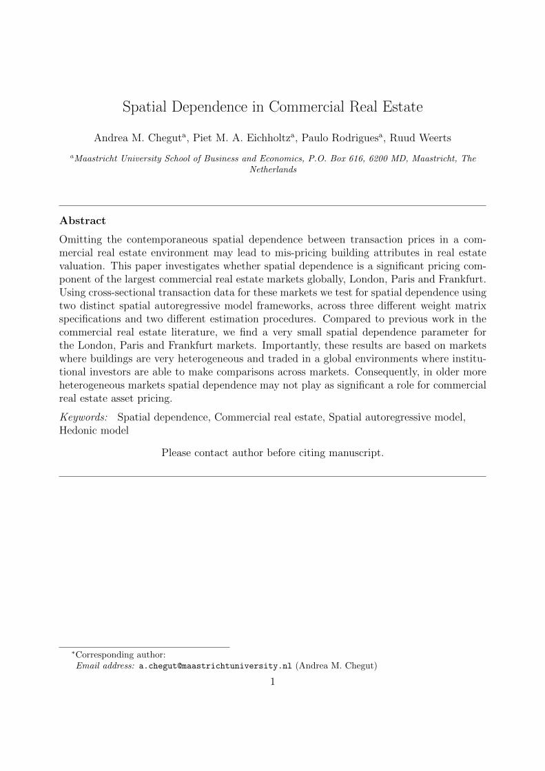
there are 242 observations. The map of these properties is shown in Figure 1.
[Figure 1 about here.]
Most of the office buildings are situated in the center. The remaining office buildings are
located in small clusters around the city center and only few buildings are is isolated from
the others. It is therefore likely to expect that most spatial dependence arises in the city
center. The office buildings in the suburbs are unlikely to show much spatial dependence as
the distance between the center and the suburbs is relatively large. The descriptive statistics
for the office market in Frankfurt are shown in Table 2.
[Table 2 about here.]
The average price of an office building in Frankfurt is e85.5 M. The most expensive build-
ings are located in the proper market, where also the largest transaction took place. The
transaction of almost 1 billion Euro is a large huge multi-tenant building sold by Morgan
Stanley in 2007. The largest transaction in 2011 was the Deutsche Bank Twin Towers. The
average value of an office building in the suburbs is with e41.7 M substantially less than the
value of the office buildings in both the city center and the proper market. Moreover is the
average size relatively smaller in this area. Most notably are the number of transactions over
the years. RCA registered the most transactions in 2006 and 2007, a period that was known
15

at the top of the market. The number of transactions decreased to 7 in 2009, which can
be directly related to the consequences of the financial crisis. The number of transactions
increases from 2010. Besides this, the average value of a transacted asset increases as well
in 2010, implying that only the most valuable assets tended to transact in this period of
uncertainty.
4.2. The Office Market in London
The London office market is characterized by its dynamics. This can be seen by the
year to year differences in take-up, supply, prime rent, investment yield, etc. The office
market relies heavily on foreign investors and is therefore heavily exposed to global economic
conditions. In 2012, the yields are at an all time low3. This implies that the London
office market is considered safe during these times of financial distress. The financial sector
dominated the office market until 2011, the year that the TMT-sector4 became a larger
occupier of the London office buildings.
The office market in London is the largest market under scrutiny. The London market
is divided into 10 sub-markets. The immense size of the office market in London makes
it harder to define the actual city center as there are more important centralized locations
that contain many office buildings. In fact, the city center in London contains three central
points where multiple office buildings tend to cluster. This is shown in Figure 2.
[Figure 2 about here.]
Clearly, most buildings in the database are located in West End. However, there is another
cluster in the market City Core. The remaining assets are more or less equally divided in
distance around the city center. Based on this map, it is likely to expect that the spatial
dependence arises in the city center. The buildings are situated close to each other and
therefore the value of the assets are likely to be influenced by the value of neighbouring assets.
Also, the value of the buildings around the city center are not likely to affect the value of the
3Market data can be found in ’European Office Market 2012’, BNP Parisbas4Technology, Media, Telecommunication sector
16

buildings in the city center for two reasons. Firstly, the distance is relatively large. Spatial
models are based on, among others, the assumption that the spatial dependence shows a
decay when the distance becomes larger. Secondly, they are not located in clusters which
implies that they do not face direct competition from their neighbouring assets. Hence, the
spatial dependence is more likely to stay in the city center itself. The descriptive statistics
are shown in Table 3.
[Table 3 about here.]
The market in London shows a lot of variation in the observations. The smallest trans-
action value is approximately e750k while the largest transaction value is almost e1.8 Bln,
which is a large shopping center in the UK partly owned by the Dutch pension fund APG.
West End is by farthest the market and contains 528 transactions. City Core contains 338
transactions, which is the second largest amount. Most notably is the average transaction
value in the Docklands. This market contains only 26 transaction but the average value is
close to e270 Mln. This can be explained by the fact that this was once the largest dock
in the world. The main docks are now no longer situated in the city center and conse-
quently this area emerged as the central business area after the immense redevelopment of
the area. The first peak of the number of transactions is in 2007. After 2007 the number of
transactions decreases substantially but the market shows a quick recovery. The number of
transaction becomes even larger in 2010 and 2011. The market in London shows signs of a
dynamic market and there is likely to be spatial dependence in the central areas. The main
activity takes place in the City Core and West End.
4.3. The Office Market in Paris
The office market in Paris is known for its dynamics. Yet, the prime rents remain
relatively stable. The take up follows the economic business cycle naturally, which is a sign
that the market is relatively liquid. Lately, the market has become a safe haven for cash
rich investors such as insurance companies and pension funds. The decline after the crisis
hit Europe is less severe than the other two markets of interest. This might imply that the
17
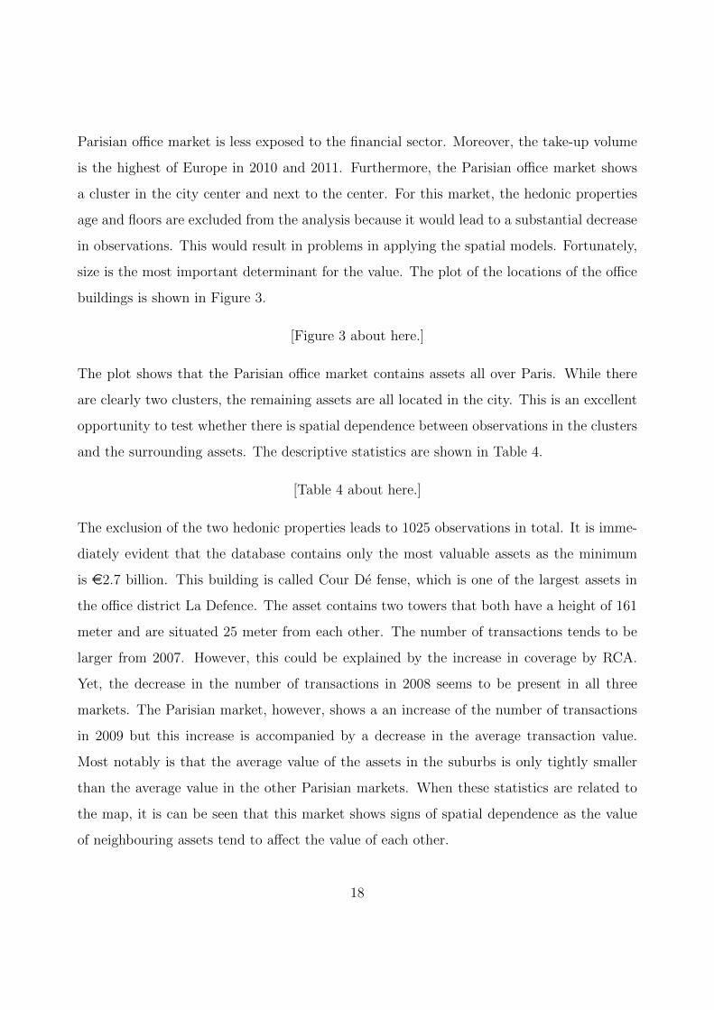
Parisian office market is less exposed to the financial sector. Moreover, the take-up volume
is the highest of Europe in 2010 and 2011. Furthermore, the Parisian office market shows
a cluster in the city center and next to the center. For this market, the hedonic properties
age and floors are excluded from the analysis because it would lead to a substantial decrease
in observations. This would result in problems in applying the spatial models. Fortunately,
size is the most important determinant for the value. The plot of the locations of the office
buildings is shown in Figure 3.
[Figure 3 about here.]
The plot shows that the Parisian office market contains assets all over Paris. While there
are clearly two clusters, the remaining assets are all located in the city. This is an excellent
opportunity to test whether there is spatial dependence between observations in the clusters
and the surrounding assets. The descriptive statistics are shown in Table 4.
[Table 4 about here.]
The exclusion of the two hedonic properties leads to 1025 observations in total. It is imme-
diately evident that the database contains only the most valuable assets as the minimum
is e2.7 billion. This building is called Cour De fense, which is one of the largest assets in
the office district La Defence. The asset contains two towers that both have a height of 161
meter and are situated 25 meter from each other. The number of transactions tends to be
larger from 2007. However, this could be explained by the increase in coverage by RCA.
Yet, the decrease in the number of transactions in 2008 seems to be present in all three
markets. The Parisian market, however, shows a an increase of the number of transactions
in 2009 but this increase is accompanied by a decrease in the average transaction value.
Most notably is that the average value of the assets in the suburbs is only tightly smaller
than the average value in the other Parisian markets. When these statistics are related to
the map, it is can be seen that this market shows signs of spatial dependence as the value
of neighbouring assets tend to affect the value of each other.
18

5. Results
Results for the transaction based SAR model and the SARAR model for the Frankfurt,
London and Paris office markets are reported below. We operationalize the models using
three different specifications of the spatial weight matrix.
5.1. Frankfurt
The dataset of the office market in Frankfurt is the smallest sample of the three markets
under scrutiny. Due to the small amount of observations in 2000, 2001 and 2002 and the
lack of observations in 2003 and 2004 it is only possible to construct an index from 2005 till
2012. Table 5 contains the results of the office market in Frankfurt.
[Table 5 about here.]
The results in Table 5 show that all the models have a relatively high explanatory power
according to the R2 measure. Most notably are the results of the SARAR model with the
spatial weight matrix specified as the contiguity matrix. The R2 is substantially smaller and
the variance is higher than the other specifications, which indicates that this combination
performs worse in explaining the transaction price.
Not all the time dummies are significant, which is against the expectations. Especially
the years 2007 and 2008 are problematic. The remaining years have a higher explanatory
power, implying that the models are able to explain the transaction prices better for these
years.The location dummies are only significant and negative for the suburbs.
The spatial dependence is limited in the present results. In the SAR-model with the
inverse distance matrix with no cut off the spatial dependence is slightly negative and sig-
nificant. This is also true for the SARAR-model with the similar matrix. This finding implies
that the spatial dependence is related to the distance. When the distance becomes larger,
the transaction value is positively affected. This makes intuitively sense as the value is likely
to depend on the buildings that are relatively close. The SARAR-model with the contiguity
matrix finds spatial dependence in the disturbance structure, which is both significant and
19

unstable. This implies that the unobserved variables affect the value of neighbouring ob-
servations but do not converge to a certain constant distribution. Consequently the results
cannot be used for either forecasting purposes or the construction of an index. The other
specifications of the spatial weight matrices are able to deal with this dependence in such a
way that the dependence arises in the spatial lag, which implies that there is weak evidence
of spatial autocorrelation.
Compared to the estimation via OLS, only the SARAR model seems to be substantially
different. Yet, the difference is mainly in the t-statistics and not in the coefficients. Based
on these results it is clear that, considering the explanatory power, the variance and the
coefficients that the spatial weight matrix, when specified as the inverse distance matrix
with no cut-off, performs better than the other specifications.
5.2. London
The sample of the office market in London is the largest of all three markets. This sample
is sufficient to construct an index that starts in 2001 and ends in 2012. The results in Table
6 show the outcomes of the regression models as laid out in the methodology.
[Table 6 about here.]
The results in Table 6 indicate that all the models with the respective specification of the
spatial weight matrix have similar explanatory power according to the R2 measure and the
variances. Yet, the estimation via OLS seems to suffer from the fact that only one hedonic
property has been taken into account. This results in insignificant parameters, even for the
time dummies. The spatial models, however, seem to find that all the year dummies are
significant.The locational dummies behave as expected, considering that the city center is
chosen as the reference location. The output shows that the Docklands is the most expensive
location while the outer region of London is the cheapest.
The spatial dependence in London is limited. Only the SAR model in combination with
the spatial weight matrix with no cut-off finds significant spatial dependence. The parameter
is, however, close to zero. The combination of the SARAR-model and the contiguity matrix
20

results again in significant spatial dependence in the disturbance structure5.
5.3. Paris
Table 7 shows the results of the Parisian market from 2001 till 2012. The sample of
the Parisian market is a little bit smaller than the sample of the London market. Yet,
this market is convenient to analyse the differences of the models in their behaviour in the
analysis of larger samples.
[Table 7 about here.]
The results in Table 7 indicate that all the models have a relatively low R2 around
the 0.40. This is due to the inclusion of only one hedonic property, the size. Again, the
coefficients for the time dummies are considerably larger in the spatial models, implying
that these models handle the small quantity of hedonic properties better. The locational
dummies behave as expected. The assets in the suburbs have a significant lower transaction
value than the assets in the suburbs. The proper market is again not significant. The
transaction value is as expected lower in the suburbs.
The spatial dependence is present in both models. In the SAR-model with the spatial
weight matrix, specified as the inverse distance matrix with no cut-off, the spatial lag is
significant and negative. This implies that there is a slight dispersion between the spatial
component and the transaction price. In other words, when the distance becomes larger the
value increases as well. The negative sign is due to the inverse distance matrix. The spatial
effect in the disturbance structure of the SARAR-model with the matrix M2 is significant
and unstable. This again reveals the problem regarding the high level of heterogeneity in
the real estate market.
5When the estimation is performed using only the office buildings in the database, the coefficient becomeslarger than 2 and thereby violating the stability condition. This again indicates that the variance does notconverge to a constant variance and the model is unstable. This is consistent with the findings in Frankfurtand indicates a large extent of heterogeneity.
21
6. Comparative Model Specifications
Both models capture spatial dependence in two distinct ways. First, the SAR has a
spatial lag. In contrast, the SARAR model contains not only the spatial lag but also
a spatial component in the disturbance structure. The significance of the parameters of
these components determines to what extent the components affect the estimation of the
parameters of the explanatory variables. When for example the parameter of the spatial
component in the disturbance structure is insignificant but the coefficient of the spatial lag is,
the SARAR model is essentially similar to the SAR model. In the case where coefficients of
the spatial lag are similar in both models, the parameters should be equal as the underlying
data is exactly the same.
6.1. Spatial Weight Matrices
The specification of the spatial weight matrices seems to affect the estimation. First,
the contiguity matrix is not able to capture the spatial dependence in the form of a spatial
lag very well. The parameters are either insignificant or the parameter is significant but
has a value close to zero. The contiguity matrix is, however, able to capture significant
spatial dependence in the disturbance structure. In fact, the use of the contiguity matrix
not only results in significant spatial dependence in the disturbance structure, but also is
significant for the spatial dependence in the spatial lag. Yet, the parameter is greater than
1 in absolute value and therefore not stable. Second, the inverse distance matrix with no
cut-off seems to perform consistently in the analysis. Both models find parameters that
are quite similar to each other. Only the parameter of the spatial lag in the model used
for the market in Frankfurt varies slightly. This seems to affect the coefficients for the
explanatory variables in the model as well. The coefficients for the explanatory variables are
slightly smaller when the SARAR model is used. Overall, the inverse distance matrix with
no cut-off performs well in capturing the spatial dependence. Thirdly, the inverse distance
matrix with a cut-off performs different than the other two specifications. The cut-off only
takes the office buildings within a circle of 5 miles into account. The parameter for the
spatial lag is insignificant for the market in Frankfurt, but is significant for the markets in
22

London and Paris. The negative sign implies that the value of an asset increases when the
distance to other assets becomes larger, which is a relevant effect as it is robust with the
other specifications.
6.1.1. The robustness of the econometric specifications
To compare the two model specifications it is convenient to look at the explanatory
power, the variances and the signs of the parameters. Comparing the results of the three
different markets it is shown that the explanatory power is approximately equal for both
models in the respective market. Additionally, the variances are approximately similar as
well. The coefficients are not only similar in sign but also in magnitude. This implies that
both models perform similar in capturing the affect of the explanatory variables. Thus,
considering the results in the preceding section it is shown that the models are robust to
each other. However, if the models perform exactly the same they would result in exactly
the same coefficients and consequently in similar indices as well. Yet, besides the small
differences, all the models seem to result in a similar path. Thus, based on the coefficients
and the indices it can be concluded that all the models are able to give some credence for
incorporating spatial dependence, but keeping in mind that the parameters are very small
for these markets.
7. Conclusion
Compared to previous work in the commercial real estate literature, we find a very small
spatial dependence parameter for the London, Paris and Frankfurt markets. Importantly,
these results are based on markets where buildings are very heterogeneous and traded in
a global environments where institutional investors are able to make comparisons across
markets. Consequently, in older more heterogeneous markets spatial dependence may not
play as significant a role for commercial real estate asset pricing.
However, consistent with LeSage and Pace (2008); Tu et al. (2004) the findings here
indicate that the coefficients in particular, are enhanced by the inclusion of the spatial de-
pendence parameter. Indicating that spatial dependence parameter is potentially an omitted
23

variable. However, the spatial dependence parameter has a very small coefficient in all mar-
kets, across all models and weight matrix specifications. Furthermore, Tu et al. (2004)
acknowledge that the lack of transactions can be problematic. Within this sample, data
problems became evident in the application of the spatial models on the office market in
Frankfurt in two forms. Firstly, the lack of transactions required the exclusion of the years
2000-2005. Secondly, the results regarding the temporal effects were weak. The problem
was also evident in the Parisian office market but only in the earlier years 2000-2004. The
remaining data was sufficient to analyse the remaining years.
Nappi-Choulet and Maury (2009) find strong evidence of spatial dependence in the
Parisian office market. Their research was, however, limited to the central business dis-
trict and La Defence. By taking the whole Parisian office market into account, the evidence
of spatial dependence was limited here. The analysis using the SARAR-model addresses
this issue by modelling spatial dependence in the error structure. Although this appears
to be a problem when the contiguity matrix is used, it cannot be responsible for the huge
differences between the findings of Nappi-Choulet and Maury (2009) and these results be-
cause the parameter of the spatial lag is similar in the SAR model. The largest difference
is from the focusNappi-Choulet and Maury (2009) on the two main business districts while
this empirical work focuses on the whole Parisian office market.
In addition, Tu et al. (2004) find differences in the indices between an OLS estimation and
the spatial model are not constant. This is consistent with the findings here and implies that
the spatial bias is not constant. This implies that the transaction value of office buildings is
different affected by the location in space across time. It is possible to allow for time-varying
parameter to take this phenomenon into account (Kuethe et al., 2008). Additionally, small
samples can impact the estimation as well. This is in line with the findings of Wong et al.
(2012) who show that spatial dependence varies with trading volume.
Future research should test an additional model, it appears that the current literature in
commercial real estate already prefers a spatio-temporal based autoregressive model. This
may be due to the findings of a strong and significant spatial dependence parameter in
these models. However, it appears for these empirical specifications that spatial dependence
24

does not have the magnitude previously expected. Thus, going forward comparisons across
three models may be important for understanding the “spatial dependence” in European
commercial real estate markets.
25

References
Anselin, L., 1988. Spatial Econometrics: Methods and Models. Studies in Operational Regional Science.
Springer.
Baltagi, B. H., Li, D., 2001. Lm tests for functional form and spatial error correlation. International Regional
Science Review 24 (2), 194–225.
Baltagi, B. H., Song, S. H., Koh, W., 2003. Testing panel data regression models with spatial error correla-
tion. Journal of econometrics 117 (1), 123–150.
Colwell, P. F., Munneke, H. J., Trefzger, J. W., 1998. Chicago’s office market: Price indices, location and
time. Real Estate Economics 26 (1), 83–106.
Debrezion, G., Pels, E., Rietveld, P., 2007. The impact of railway stations on residential and commercial
property value: A meta-analysis. The Journal of Real Estate Finance and Economics 35 (2), 161–180–.
URL http://dx.doi.org/10.1007/s11146-007-9032-z
Downs, D. H., Slade, B. A., 1999. Characteristics of a full-disclosure, transaction-based index of commercial
real estate. Journal of Real Estate Portfolio Management 5 (1), 95 – 104.
Elhorst, J. P., 2001. Dynamic models in space and time. Geographical Analysis 33 (2), 119–140.
Elhorst, J. P., 2010a. Applied spatial econometrics: Raising the bar. Spatial Economic Analysis 5 (1), 9–28.
Elhorst, J. P., 2010b. Spatial panel data models. In: Fischer, M. M., Getis, A. (Eds.), Handbook of Applied
Spatial Analysis. Springer Berlin Heidelberg, pp. 377–407.
Elhorst, J. P., Lacombe, D. J., Piras, G., 2012. On model specification and parameter space definitions in
higher order spatial econometric models. Regional Science and Urban Economics 42 (1), 211–220.
Fisher, J. D., Geltner, D. M., Webb, R. B., 1994. Value indices of commercial real estate: A comparison of
index construction methods. The Journal of Real Estate Finance and Economics 9, 137–164.
Geltner, D., Pollakowski, H., September 2007. A set of indexes for trading commercial real estate based on
the real capital analytics transaction prices database, release 2.
Kelejian, H. H., Prucha, I. R., 1997. Estimation of spatial regression models with autoregressive errors by two
stage least squares procedures: A serious problem. Electronic working papers, University of Maryland,
Department of Economics.
Kelejian, H. H., Prucha, I. R., 1999. A generalized moments estimator for the autoregressive parameter in
a spatial model. Electronic Working Papers 95-001, University of Maryland, Department of Economics.
Kelejian, H. H., Prucha, I. R., 2010. Specification and estimation of spatial autoregressive models with
autoregressive and heteroskedastic disturbances. Journal of Econometrics 157 (1), 53 – 67.
Kuethe, T. H., Foster, K. A., Florax, R. J., 2008. A spatial hedonic model with time-varying parameters: A
new method using flexible least squares. 2008 Annual Meeting, July 27-29, 2008, Orlando, Florida 6306,
American Agricultural Economics Association (New Name 2008: Agricultural and Applied Economics
26

Association).
Lee, L.-F., November 2004. Asymptotic distributions of quasi-maximum likelihood estimators for spatial
autoregressive models. Econometrica 72 (6), 1899–1925.
LeSage, J. P., Pace, R. K., 2008. Spatial econometric modeling of origin-destination flows*. Journal of
Regional Science 48 (5), 941–967.
LeSage, J. P., Pace, R. K., 2010. Spatial econometric models. In: Fischer, M. M., Getis, A. (Eds.), Handbook
of Applied Spatial Analysis. Springer Berlin Heidelberg, pp. 355–376.
Miles, M., McCue, T., 1984. Commercial real estate returns. American Real Estate and Urban Economics
Association Journal 12 (3), 355 – 377.
Nappi-Choulet, I., Maleyre, I., Maury, T., 2007. A hedonic model of office prices in paris and its immediate
suburbs. Journal of Property Research 24 (3), 241–263.
Nappi-Choulet, I., Maury, T.-P., 2009. A spatiotemporal autoregressive price index for the paris office
property market. Real Estate Economics 37 (2), 305–340.
Pace, R. K., Barry, R., Clapp, J. M., Rodriquez, M., 1998. Spatiotemporal autoregressive models of neigh-
borhood effects. The Journal of Real Estate Finance and Economics 17 (1), 15–33.
URL http://dx.doi.org/10.1023/A:1007799028599
Pace, R. K., Barry, R., Gilley, W., Sirmans, C., 2000. A method for spatial-temporal forecasting with an
application to real estate prices. International Journal of Forecasting 16 (2), 229 – 246.
Rosen, S., 1974. Hedonic prices and implicit markets: Product differentiation in pure competition. Journal
of Political Economy 82 (1), 34–55.
URL http://ideas.repec.org/a/ucp/jpolec/v82y1974i1p34-55.html
se Can, A., Megbolugbe, I., 1997. Spatial dependence and house price index construction. The Journal of
Real Estate Finance and Economics 14, 203–222, 10.1023/A:1007744706720.
Tu, Y., Yu, S.-M., Sun, H., 2004. Transaction-based office price indexes: A spatiotemporal modeling ap-
proach. Real Estate Economics 32 (2), 297–328.
Wong, S., Yiu, C., Chau, K., 2012. Trading volume-induced spatial autocorrelation in real estate prices. The
Journal of Real Estate Finance and Economics, 1–13.
27

List of Figures
1 Frankfurt office market . . . . . . . . . . . . . . . . . . . . . . . . . . . . . . 292 London office market . . . . . . . . . . . . . . . . . . . . . . . . . . . . . . . 303 Parisian office market . . . . . . . . . . . . . . . . . . . . . . . . . . . . . . . 31
28

Figure 1: Frankfurt office market
29

Figure 2: London office market
30

Figure 3: Parisian office market
31

List of Tables
1 The general null-hypotheses . . . . . . . . . . . . . . . . . . . . . . . . . . . 332 The office market in Frankfurt . . . . . . . . . . . . . . . . . . . . . . . . . 343 The office market in London . . . . . . . . . . . . . . . . . . . . . . . . . . 354 The office market in Paris . . . . . . . . . . . . . . . . . . . . . . . . . . . . 365 The office market in Frankfurt . . . . . . . . . . . . . . . . . . . . . . . . . 376 The office market in London . . . . . . . . . . . . . . . . . . . . . . . . . . 387 The office market in Paris . . . . . . . . . . . . . . . . . . . . . . . . . . . . 39
32

Table 1: The general null-hypotheses
Hypothesis Formulation
H1 The parameter ρ is zero.H2 The parameter λ is zero.H3 The parameters βn are zero.
33

Table 2: The office market in Frankfurt
Variable Mean Sigma Min Max n
TotalPrice 85,455,294 135,089,430 2,925,902 956,422,074 242Size(sq ft) 188,953 222,204 11,291 1,959,032 242
Submarkets (Prices)City center 97,959,529 127,139,507 5,468,678 744,833,433 68Proper 113,547,394 172,125,953 2,960,367 956,422,074 93Suburbs 42,704,019 63,799,781 2,925,902 455,196,341 81
Time (prices)2006 65,436,296 85,792,849 2,960,367 513,267,792 682007 93,410,372 152,188,315 2,925,902 956,422,074 1002008 52,079,942 45,525,376 8,705,319 198,937,032 202009 61,739,976 76,150,549 3,318,175 235,248,950 72010 123,415,968 172,481,934 5,691,450 744,833,433 182011 137,911,008 224,649,845 6,488,453 853,591,989 162012 75,971,816 57,982,689 12,483,857 214,928,084 13
34

Table 3: The office market in London
Variable Mean Sigma Min Max nTotalPrice 62,056,665 105,375,944 746,776 1,742,999,999 1,284Size 102,570 157,970 107 1,899,800 1,284
Sub-markets (Prices)City Core 81,409,140 87,654,824 1,236,286 669,175,522 338City Fringe 93,723,752 228,209,472 4,073,505 1,742,999,999 66Docklands 270,339,810 345,873,170 8,659,347 1,111,900,000 26Midtown 61,755,465 68,028,395 1,450,000 302,500,000 95North Central 32,682,227 54,131,527 1,100,000 235,000,000 24Outer 25,266,281 33,100,810 3,000,000 230,000,000 91South central 55,511,333 56,001,551 5,075,000 300,000,000 47Southern Fringe 27,949,914 17,831,471 6,400,000 60,000,000 8West Central 34,608,680 65,480,137 2,800,000 480,000,000 61West End 47,454,035 68,222,336 746,776 862,693,541 528
Time (prices)2001 39,712,539 42,856,098 5,100,000 246,500,000 702002 58,464,379 65,499,265 4,753,200 238,000,000 422003 67,201,811 61,455,520 4,400,000 239,500,000 422004 87,512,716 144,057,052 4,461,841 1,111,900,000 712005 74,660,728 57,740,281 1,471,898 230,666,667 812006 74,959,575 95,158,610 2,800,000 527,000,000 972007 88,334,835 162,170,046 1,236,286 1,093,452,610 1152008 62,383,761 105,157,818 746,776 838,000,000 712009 60,845,491 70,304,067 2,465,501 445,000,000 972010 51,745,253 87,779,661 1,780,000 862,693,541 2712011 52,651,462 126,651,733 3,250,000 1,742,999,999 2512012 57,403,342 82,820,197 4,410,000 470,000,000 76
35

Table 4: The office market in Paris
Variable Mean Sigma Min Max nTotalPrice 72,823,926 130,964,036 73,134 2,747,359,885 1,025Size 109,938 208,387 126 3,713,580 1,025
Submarkets (Prices)City center 68,599,658 92,263,407 162,797 574,727,811 281Proper 78,241,290 205,305,685 204,271 2,747,359,885 212Suburbs 72,896,367 108,312,559 73,134 764,999,229 532
Time (prices)2005 61,589,965 94,031,137 2,730,022 363,630,251 912006 81,826,770 95,866,076 265,356 466,350,231 782007 100,113,497 227,809,586 146,387 2,747,359,885 1932008 53,986,118 65,429,472 182,441 341,225,662 1592009 62,462,413 89,268,202 275,142 565,360,000 1132010 63,862,630 119,873,616 73,134 764,999,229 1302011 74,981,764 92,702,938 73,781 519,076,210 1902012 72,460,875 100,651,659 3,704,001 44,4480,123 71
36

Table 5: The office market in Frankfurt
SAR SARAR OLSM1 M2 M3 M1 M2 M3 -
R-squared 0.7617 0.7666 0.7621 0.7354 0.7661 0.7621 0.7618Rbar-squared 0.7525 0.7575 0.7529 0.7251 0.757 0.7529 0.7525σ2 0.3525 0.3456 0.3521 0.3917 0.3462 0.3521 0.3678Nobs 242 242 242 242 242 242 242Nvars 10 10 10 11 11 11 10log-likelihood -133.3502 -130.9495 -133.22033Variable Coefficients (t-stat) Coefficients (t-stat) Coeff.(t-st.)
M1 M2 M3 M1 M2 M3 -constant 5.55 5.55 5.56 5.71 5.61 5.55 5.59
(10.87) (11.99) (11.79) (9.78) (10.04) (9.43) (11.71)Size 1.03 1.03 1.03 1.04 1.03 1.03 1.03
(25.18) (25.64) (25.31) (21.88) (21.64) (20.57) (24.82)2007 0.01 0.00 0.01 0.01 0.00 0.01 0.01
(1.34) (0.29) (1.36) (2.03) (0.22) (1.61) (1.31)2008 0.00 0.00 0.00 -0.01 0.00 0.00 0.00
(-0.32) (-0.43) (-0.30) (-1.01) (-0.36) (-0.21) (-0.32)2009 0.01 0.02 0.01 0.00 0.02 0.01 0.01
(1.05) (1.12) (1.06) (-0.05) (0.74) (0.70) (1.01)2010 0.02 0.02 0.02 0.01 0.02 0.02 0.02
(2.07) (2.06) (1.89) (0.81) (2.65) (2.11) (2.02)2011 0.02 0.02 0.02 0.00 0.02 0.02 0.02
(1.68) (1.74) (1.71) (-0.16) (2.05) (1.95) (1.65)2012 0.02 0.02 0.02 0.01 0.02 0.02 0.02
(1.96) (2.02) (1.98) (0.83) (1.83) (1.69) (1.91)Proper -0.01 -0.01 -0.01 -0.01 -0.01 -0.01 -0.01
(-0.91) (-1.12) (-0.91) (-1.38) (-1.19) (-0.94) (-0.91)Suburbs -0.04 -0.04 -0.04 -0.06 -0.04 -0.04 -0.04
(-6.13) (-6.39) (-5.95) (-4.34) (-6.89) (-6.21) (-6.00)ρ 0.00 0.03 0.01 0.00 0.04 0.01 -
(0.19) (2.20) (0.55) (0.19) (4.14) (0.59) -λ - - - 1.70 -1.57 -0.04 -
- - - (4.88) (-0.52) (-0.18) -
37

Table 6: The office market in London
SAR SARAR OLSM1 M2 M3 M1 M2 M3 -
R-squared 0.5961 0.5971 0.595 0.595 0.5522 0.595 0.5452Rbar-squared 0.5893 0.5904 0.5882 0.5883 0.5995 0.5882 0.5391σ2 0.5411 0.5395 0.5422 0.5422 0.5462 0.5423 0.6175Nobs 1284 1284 1284 1284 1284 1284 1284Nvars 22 22 22 23 23 23 22log-likelihood -982.6565 -980.7239 -983.98475 - - - -Variable Coefficients (t-stat) Coefficients (t-stat) Coeff. (t-st.)
M1 M2 M3 M1 M2 M3 -constant 11.33 11.35 11.26 11.26 11.53 11.27 12.29
(67.89) (68.40) (69.20) (46.37) (52.02) (47.20) (87.13)Size 0.60 0.60 0.60 0.61 0.59 0.60 0.61
(35.77) (35.26) (35.79) (20.97) (21.05) (20.80) (35.12)2002 0.04 0.04 0.04 0.04 -0.04 0.04 -0.02
(4.95) (4.98) (5.07) (5.00) (5.12) (5.26) (-2.05)2003 0.04 0.05 0.05 0.042 0.05 0.05 -0.01
(5.31) (5.49) (5.49) (5.56) (5.94) (5.79) (-1.34)2004 0.05 0.05 0.05 0.04 0.05 0.05 -0.01
(6.37) (6.85) (6.75) (6.45) (7.10) (6.94) (-1.32)2005 0.05 0.06 0.05 0.05 0.06 0.05 0.00
(7.94) (8.12) (7.94) (7.54) (8.22) (8.09) (-0.17)2006 0.05 0.06 0.06 0.05 0.06 0.06 0.00
(7.94) (8.79) (8.50) (7.76) (8.51) (8.34) (-0.12)2007 0.05 0.06 0.06 0.05 0.06 0.06 0.00
(8.10) (9.08) (8.72) (7.76) (8.70) (8.54) (-0.15)2008 0.05 0.05 0.05 0.05 0.05 0.05 -0.01
(6.38) (7.14) (6.85) (6.50) (7.32) (6.90) (-1.20)2009 0.05 0.05 0.05 0.05 0.06 0.05 -0.01
(7.19) (7.77) (7.41) (7.34) (8.16) (7.58) (-1.22)2010 0.06 0.07 0.06 0.06 0.08 0.06 -0.01
(11.23) (10.91) (11.09) (9.66) (9.53) (9.59) (-2.18)2011 0.07 0.08 0.07 0.07 0.08 0.07 0.02
(11.41) (10.77) (11.28) (10.05) (9.59) (10.05) (2.40)2012 0.06 0.07 0.06 0.06 0.07 0.06 -0.01
(8.89) (9.14) (8.74) (8.94) (8.94) (8.65) (-2.04)City Fringe -0.01 -0.01 -0.01 -0.01 -0.01 -0.01 -0.02
(-1.00) (-1.05) (-1.08) (-0.92) (-1.95) (-1.07) (-2.50)Docklands 0.02 0.02 0.02 0.02 0.02 0.02 -0.04
(2.50) (2.47) (2.47) (2.15) (2.01) (2.44) (-8.09)Midtown 0.00 0.00 0.00 0.00 -0.01 0.00 -0.01
(-0.21) (-0.35) (-0.36) (-0.06) (-1.55) (-0.42) (-1.10)North Central -0.02 -0.02 -0.02 -0.02 -0.03 -0.02 -0.04
(-2.26) (-2.39) (-2.43) (-1.48) (-2.42) (-1.93) (-2.36)Outer -0.04 -0.04 -0.04 -0.04 -0.05 -0.04 -0.01
(-7.86) (-7.72) (-7.92) (-6.10) (-7.43) (-6.55) (-1.54)South Central 0.00 0.00 0.00 0.00 -0.01 0.00 0.00
(-0.13) (-0.20) (-0.09) (-0.33) (-0.98 ) (-0.11) (-0.11)Southern Fringe -0.04 -0.04 -0.04 -0.04 -0.04 -0.03 -0.03
(-2.43) (-2.44) (-2.24) (-3.75) (-4.09) (-3.05) (-3.05 )West Central -0.01 -0.01 -0.01 -0.01 -0.01 -0.01 -0.01
(-1.03) (-1.24) (-1.21) (-1.56) (-1.96) (-1.04) (-1.04)West End 0.01 0.01 0.01 0.01 -0.04 0.01 0.01
(2.84) (2.73) (2.72) (2.52) (-2.69) (2.93) (2.93)ρ -0.01 -0.03 -0.02 -0.01 -0.04 -0.03 -
(-1.75) (-2.64) (-0.65) (-1.74) (-2.67) (-0.91) -λ - - - 0.30 0.29 0.33 -
- - - (4.16) (0.83) (0.45) -
38

Table 7: The office market in Paris
SAR SARAR OLSM1 M2 M3 M1 M2 M3 -
R-squared 0.4064 0.4142 0.4076 0.4064 0.4101 0.4076 0.4064Rbar-squared 0.4006 0.4084 0.4017 0.4005 0.4042 0.4018 0.4006σ2 1.1717 1.1576 1.1693 1.1717 1.1645 1.1694 1.1844Nobs 1025 1025 1025 1025 1025 1025 1025Nvars 11 11 11 12 12 12 11log-likelihood -1180.3667 -1174.1686 -1179.3332 - - - -Variable Coefficients (t-stat) Coefficients (t-stat) Coeff.(t-st.)
M1 M2 M3 M1 M2 M3 -constant 9.95 10.13 9.91 10.05 9.66 9.90 9.95
(30.89) (34.67) (34.06) (26.34) (24.59) (27.16) (34.24)Size 0.58 0.58 0.59 0.58 0.61 0.59 0.58
(21.97) (22.14) (22.11) (16.01) (15.86) (16.19) (21.96)2006 0.07 0.07 0.07 0.07 0.08 0.07 0.07
(7.88) (7.85) (7.91) (7.35) (6.61) (7.41) (7.84)2007 0.10 0.11 0.10 0.10 0.12 0.10 0.10
(13.15) (13.65) (13.20) (12.29) (11.14) (12.53) (13.09)2008 0.06 0.06 0.06 0.06 0.08 0.06 0.06
(7.22) (7.78) (7.26) (6.76) (6.83) (6.82) (7.19))2009 0.07 0.07 0.07 0.07 0.08 0.07 0.07
(7.82) (8.16) (7.92) (7.65) (7.30) (7.88) (7.80)2010 0.06 0.06 0.06 0.06 0.07 0.06 0.06
(6.57) (6.96) (6.62) (6.25) (6.49) (6.40) (6.59)2011 0.08 0.09 0.08 0.08 0.10 0.08 0.08
(10.01) (10.68) (10.08) (9.34) (8.87) (9.42) (10.01)2012 0.07 0.08 0.07 0.07 0.09 0.07 0.07
(7.26) (7.80) (7.27) (7.43) (7.31) (7.47) (7.24)Proper 0.00 0.00 0.00 0.00 0.00 0.00 0.00
(-0.44) (-0.45) (-0.23) (-0.53) (-0.69) (-0.24) (-0.44)Suburbs -0.02 -0.02 -0.02 -0.02 -0.02 -0.02 -0.02
(-3.55) (-3.49) (-3.58) (-3.70) (-3.98) (-3.74) (-3.53)ρ 0.00 -0.08 -0.04 0.00 -0.07 -0.05 -
(0.00) (-3.53) (-1.44) (-0.74) (-2.03) (-1.93) -λ - - - 0.01 1.98 -0.39 -
- - - (0.10) (3.75) (-0.44) -
39