Spatial Clustering of Myelodysplastic Syndromes (MDS) in ...authors.fhcrc.org/445/1/DeRoosACCCManuscript080610.pdfSpatial Clustering of Myelodysplastic Syndromes (MDS) in the Seattle-Puget

1

Spatial Clustering of Myelodysplastic Syndromes (MDS) in the Seattle-Puget Sound Region of Washington State

Michelle E Ross1, Jon Wakefield1,4, Scott Davis2,3, Anneclaire J De Roos2,3

1Department of Biostatistics, University of Washington, Seattle, WA 2Division of Public Health Sciences, Fred Hutchinson Cancer Research Center, Seattle, WA 3Department of Epidemiology, University of Washington, Seattle, WA 4Department of Statistics, University of Washington, Seattle, WA Corresponding Author: Anneclaire J. De Roos 1100 Fairview Avenue N, M4-B874 Seattle, WA 98109-1024 Phone: 206-667-7315 Fax: 206-667-4787 email : [email protected] Abbreviated title: Spatial clustering of myelodysplastic syndromes Acknowledgement of financial support: This work was supported through a contract with the Surveillance, Epidemiology, and End Results (SEER) program of the National Cancer Institute (NO1-PC-55020-20). Michelle Ross and Jon Wakefield were supported by grant R01 CA095994 from the National Institutes of Health.

2

ABSTRACT

Objectives. Incidence of myelodysplastic syndromes (MDS) has been described in the United

States since its inclusion in the Surveillance, Epidemiology, and End Results (SEER) program in

2001, and the Seattle-Puget Sound region of Washington State has among the highest rates of

the registries. In this investigation, we described small-scale incidence patterns of MDS within

the Seattle-Puget Sound region from 2002 to 2006 and identified potential spatial clusters to

inform planning of future studies of MDS etiology.

Methods. We used a spatial disease mapping model to estimate smoothed relative risks for

each census tract and to describe the spatial component of variability in the incidence rates.

We also used two methods to describe the location of potential MDS clusters: the approach of

Besag and Newell and the Kulldorff spatial scan statistic.

Results. Our findings from all three approaches indicated the most likely areas of increased

MDS incidence were located on Whidbey Island in Island County.

Conclusion. Interpretation is limited because our data are based on the residential location of

the MDS case at the time of diagnosis only. Nevertheless, inclusion of identified cluster regions

in future population-based research and investigation of individual-level exposures could shed

light on environmental risk factors for MDS.

Key words: myelodysplastic syndromes, cancer cluster, cancer registry

3

INTRODUCTION

The myelodysplastic syndromes (MDS) are a group of clonal proliferative bone marrow

disorders that result in dysmyelopoiesis and peripheral blood cytopenias [1]. The course of

disease is characterized by gradual and cumulative damage inflicted by persistent cytopenias

which may result in resistance to transfusions and an overall deterioration of the immune

system [2]. In approximately 30% of patients, MDS transforms to acute myeloid leukemia

(AML).

Despite the serious health outcomes of MDS, little is known about its causes. The few

known risk factors include radiation or chemotherapy treatment for a previous malignancy, and

occupational exposure to benzene [3,4]. It has also been suggested that the initial event in

MDS may be infectious [2]. There have been very few epidemiologic studies of MDS, primarily

because of its previous non-inclusion in population-based cancer registries; however, recent

changes in MDS reporting have facilitated identification of MDS cases for research. Starting in

2001, a requirement was put in place for reporting of MDS to cancer registries of the

Surveillance, Epidemiology, and End Results (SEER) program of the United States. Since that

time, the incidence of MDS was estimated from U.S. cancer registry data at approximately 3.3

incident cases per 100,000 persons per year for 2001-2003 [5].

There has been considerable geographic variability of estimated MDS incidence

between the SEER 9 registries, with the age-sex-race-adjusted annual incidence rate of MDS in

2001-2006 ranging from 2.8-2.9 per 100,000 (Hawaii, San Francisco-Oakland SMSA and

Atlanta Metropolitan) to 5.9-6.2 per 100,000 (Detroit Metropolitan and Seattle-Puget Sound) [6].

Differential reporting completeness likely plays a role in the geographic discrepancies; however,

true regional differences in incidence are also possible and could result from differing lifestyle or

spatially-determined exposure to environmental or infectious agents. Within-region small-scale

geographic clustering identified through surveillance may suggest specific geographic areas for

further investigation. This approach has been pursued to only a limited extent. For example, a

4

significant geographic cluster of MDS involving 41 MDS cases diagnosed from 2001-2003 within

46 census tracts was detected in western Connecticut using a spatial scan statistic [7]; however,

potential causes of this cluster were not investigated.

The aims of our study were to investigate geographic clustering of incident MDS and to

identify the location of potential clusters, among cases reported to the SEER program in the

Seattle-Puget Sound region of Washington State. To this end, we identified potential spatial

clusters using several methods and carried out regression analyses to explore ecological

associations of MDS incidence with census variables. The overall purpose of our analysis was

to describe small-scale spatial incidence patterns of MDS within our region and to identify

potential clusters of MDS in order to inform planning of future population-based studies of MDS

etiology.

MATERIALS AND METHODS

Data Description

We obtained data from the Cancer Surveillance System of the SEER program on

incident cases of MDS diagnosed in 13 counties of the Seattle-Puget Sound region in 2002-

2006. Although MDS was reportable starting in 2001, we did not include 2001 in our analysis

because the number of cases increased considerably from 2001 than 2002 (by 28%), indicating

a possible lag in acclimating to the reporting requirement – a point that has also been noted at

the national level [5]. MDS cases were identified by ICD-O-3 code [8], and included the

histologic subtypes refractory anemia (RA, ICD-O-3 9980), refractory anemia with sideroblasts

(RAS, ICD-O-3 9982), refractory anemia with excess blasts (RAEB, ICD-O-3 9983), refractory

anemia with excess blasts in transformation (RAEB-t, ICD-O-3 9984), refractory cytopenia with

multilineage dysplasia (RCMD, ICD-O-3 9985), MDS with 5q deletion (5q- syndrome, ICD-O-3

9986), therapy-related MDS, NOS (ICD-O-3 9987), and MDS, NOS (ICD-O-3 9989).

5

The dataset for the cluster investigation consisted of 1238 cases, among whom there

was adequate residential information with which to assign census tract for 1225 cases; these

cases comprised the study population for our analysis. Case counts within each of the 887 U.S.

Census tracts in the study area were stratified by sex, age (<50, 50-54, 55-59, 60-64, 65-69, 70-

74, 75-79, 80-84, ≥85), and race (white versus non-white). The case counts data were

combined with U.S. Census data from 2000 [9] of population counts within each census tract

stratified by age, sex and race in the same categories as the cases.

Statistical Analysis

We investigated clustering among all MDS cases and among first primary MDS cases

(i.e., MDS cases with no previous cancer diagnosis), separately, because of the possibility that

spatially-determined environmental and/or infectious exposures may be more etiologically

relevant for first primary MDS than for all MDS (a group which includes MDS cases with

previous cancer diagnoses, whose incident MDS may or may not have been caused by

previous chemotherapy and/or radiation treatment). Nevertheless, we considered both

analyses in line with the aims of our investigation, as spatially-dependent exposures could

theoretically contribute to MDS etiology, regardless of whether a person had a previous cancer

diagnosis – particularly for those with longer latency between their previous cancer and MDS

diagnosis. It was not our intention to test differences in the results for all MDS and first primary

MDS, as one is a large subset of the other; rather, we sought to describe MDS clustering to

guide future research. We also conducted post hoc analyses of clustering within the subgroup

of MDS patients with a previous cancer (identified based on information reported to SEER), to

glean the extent to which clusters identified among both all MDS and first primary MDS were

due solely to patterns among first primary MDS. However, we did not seek to identify new

clusters among MDS patients with a previous cancer, because this group was small and thus

power was limited.

6

Our study is exploratory in nature and we consequently employed complementary

methods to investigate clustering of MDS cases and to identify the location of geographic

clusters. The spatial modeling was carried out using the WinBUGS software [10], and cluster

detection was conducted using the R software version 2.4.1.

Disease mapping (ICAR)

We used a popular disease mapping approach that allows both examination of spatial

clustering of incident disease, and the incorporation of potential predictor variables using an

intrinsic conditional autoregressive (ICAR) model. The basic model for the case counts is

defined as:

( )i i iY Poisson Eθ , (1)

where iY is the number of cases in area i, iE is the number of expected cases in area i, and iθ

is the relative risk of disease associated with area i. The maximum likelihood estimate (MLE)

/ ,i i iY Eθ = corresponds to the standardized incidence ratio (SIR) and gives an estimate of the

area-level (census-tract-level) relative risk in area i. The variance of the MLE is proportional to

1/ iE and so areas with small expected numbers can show large variability in their relative risk

estimates. To overcome this instability, we specified a random effects model in which we

allowed both global and local smoothing. Specifically the model was given by:

0log ,i i iU Vθ β= + + (2)

where global shrinkage was achieved through the independent random effects,

2(0, )i ind VV N σ , and the Ui were random effects with a spatial structure. We modeled

1( , , )nU U U= K with a so-called intrinsic conditional autoregressive (ICAR) prior:

2| , ( , / ),ii j i U iU U j N U mδ ω∈

7

where iδ was the set of neighbors (census tracts) of area i, im was the number of

neighbors,⎯ iU was the mean of the spatial random effects of the neighbors, and 2Uω was the

conditional variance whose magnitude determined the amount of spatial variation. This model

imposes smoothing by assuming that the spatial effect in a particular area is similar to the mean

of the spatial effects in close-by areas, with the strength of similarity determined by the number

of neighbors (so that the similarity imposed is stronger for an area with more neighbors). In our

analysis, census tracts i and j were defined to be neighbors if they share a common boundary.

With this definition and based on the distance between certain areas located in the Seattle-

Puget Sound region and separation by bodies of water, we defined census tracts located in San

Juan County to only have neighbors in San Juan County. In addition, census tracts located in

Island County with neighboring relationships that crossed the Admiralty Inlet (which lies

between Whidbey Island and the northeastern mainland of the Olympic Peninsula) were broken.

We conducted post hoc exploratory analyses using an alternative neighborhood structure in the

ICAR model which retained neighbor links between census tracts located on islands and on the

mainland. This dramatically reduced the proportion of the variability that was spatial in nature

as well as the standard deviation of the spatial random effects. However, it did not substantially

change the range of the residual relative risks for MDS incidence, nor the locations of elevated

relative risks; therefore, we only present results from our neighborhood structure defined a

priori.

There are two variances in the random effects model, one spatial and one non-spatial,

but they are not directly comparable since 2Uω is a conditional variance while 2

Vσ is a marginal

variance. To make the variances comparable, we calculated an approximate spatial marginal

variance, 2Uσ . As in Wakefield (2007) [11], we placed the inverse gamma prior with parameters

8

1 and 0.026 on the total variance distribution, 2 2U Vσ σ+ , and a uniform prior on the proportion of

variance that is spatial,

p= 2Uσ /( 2 2

U Vσ σ+ ).

This inverse gamma prior ensures that the residual relative risks, exp( )i iU V+ , fall between 0.5

and 2, with 95% probability. Once fitted, model (2) may inform on the level of geographical

residual risk in area i through examination of Ui and Vi, the absolute amount of residual

variability through 2 2U Vσ σ+ , the proportion of the total variability that is spatial via the estimate of

p, and the location of areas with increased risk. Areas with potentially increased risk were

highlighted as those in which the posterior probability (pp) that the relative risk (RR) exceeded

1.2 in the census tract was greater than 0.7.

We further investigated potential ecologic determinants of the geographical distribution

of MDS cases by carrying out ecological spatial regression using several census-tract-level

demographic variables from the 2000 U.S. Census [9]; namely, median household income

(scaled and continuous), education (proportion of population with a bachelor’s degree), race

(proportion white, black, Asian, other), Hispanic ethnicity (proportion), housing density (scaled

and continuous), and urbanicity (Rural-Urban Continuum Code [RUCA] code categorized as

urban=1-3, suburban=4-6, rural=7-10). The regression was carried out by extending the

disease mapping described above via

0log Ti i i iX U Vθ β β= + + + ,

where the iX are a vector of area-level risk factors associated with census tract i, and exp( )β

are the corresponding ecological relative risks. We evaluated associations between the census

variables and MDS incidence rates by examination of the log relative risks and 95% intervals.

9

Cluster detection

We used two methods to investigate whether there were clusters present, one due to

Besag and Newell [12], and one due to Kulldorff [13]. A number of approaches to cluster

detection have been proposed, the most popular of which is that of Kulldorff, due in no small

part to the availability of the user-friendly SatScan software. We chose to additionally apply the

method of Besag and Newell since it has the ability to detect rural clusters that may be missed

by the Kulldorff method, due to the sparse populations in rural areas. In each method, circles

are centered upon census tract centroids [9], and the significance of the number of cases within

each circle is determined. The methods differ in the manner in which the circles are defined and

in the way they report clusters, as we now describe.

Besag and Newell. In the method of Besag and Newell (1991) [12], circles are defined

by containing a number, k, of cases, and all circles containing that number of cases are drawn.

In the version we implement we use each census tract as a circle center, regardless of whether

the census tract contains a case or not. As the circle expands to contain the required number of

cases, a census tract is included in the circle if its centroid lies within the circle, so that jagged

circles result. The number of expected cases is then derived, based on the observed

population, and a p-value is calculated assuming the cases within the circles follow a Poisson

distribution by summing over areas. Hence, a cluster size, k, needs to be decided upon. The

method of Besag and Newell was originally designed for finding small clusters. In the example

considered in Besag and Newell [12], there were 496 cases in 16183 areas, and the authors

chose to search for potential clusters of sizes k=2,4,6,8. We have more cases (1225 MDS

cases) in fewer areas (887 census tracts); however, the total population sizes are similar.

Hence, we chose k=10. The Besag and Newell method does not control for multiple testing, so

we did not want to consider more than one value of k.

Due to the large multiple testing problem with the Besag and Newell method, we chose a

significance threshold of 0.005 – lower than that conventionally chosen. Given that there are

10

887 geographic areas, this means that if all nulls were true (i.e., the cases are randomly

distributed across the study region within each of the strata of the study population), the

expected number of falsely identified clusters would be 4. There is an additional problem of

non-independence of tests, which is not dealt with by the method. In general, positive

dependence in test statistics leads to a conservative test, with a loss of power.

Spatial scan statistic. In the spatial scan statistic approach to cluster detection

described by Kulldorff [13], circles are centered on the centroids of each census tract, and are

defined in differing sizes defined by inclusion of different proportions of the underlying

population, ranging between zero and the specified maximum of up to 50% of the population.

For each circle, the observed and expected numbers of cases inside and outside the circle are

calculated. A likelihood ratio statistic is calculated based on the null hypothesis that the relative

risk of disease inside the circle is the same as that outside the circle and the alternative

hypothesis that the relative risk of disease inside the circle is greater than that outside the circle

(a Poisson likelihood is assumed). The maximum of these statistics (i.e., the most likely of all

the clusters) is then used as the overall test statistic, and we assess its significance level using

a Monte Carlo procedure in which we simulate data under the null [7]. We performed 99,999

replications for each test. Hence, in contrast to the Besag and Newell method, the multiple

testing and dependency issues are addressed via the Monte Carlo procedure. The Kulldorff

method cannot formerly address whether secondary clusters are significant, however.

RESULTS

The 13-county study area that comprises the SEER Seattle-Puget Sound region in Western

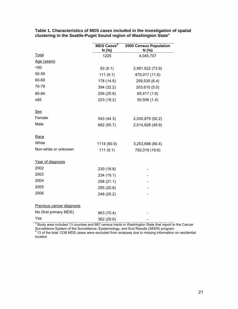
Washington is shown in Figure 1. Characteristics of the 1225 MDS cases and the general

population in the study area are shown in Table 1. MDS cases were generally age 70 or older

(71.3%) and white (90.9%). The age distribution of the general population was considerably

younger than MDS cases. The general population was also more likely to be of nonwhite or

11

unknown race compared to MDS cases. Of the MDS patients, 362 had been diagnosed with a

previous cancer (29.6%), and 863 (70.4%) had not (first primary MDS).

All MDS

There was not a great deal of residual variability in relative risk estimates for MDS

incidence using the disease mapping (ICAR) approach, indicating that there is not a large

amount of excess Poisson variation, spatial or otherwise (a 95% range for the residual relative

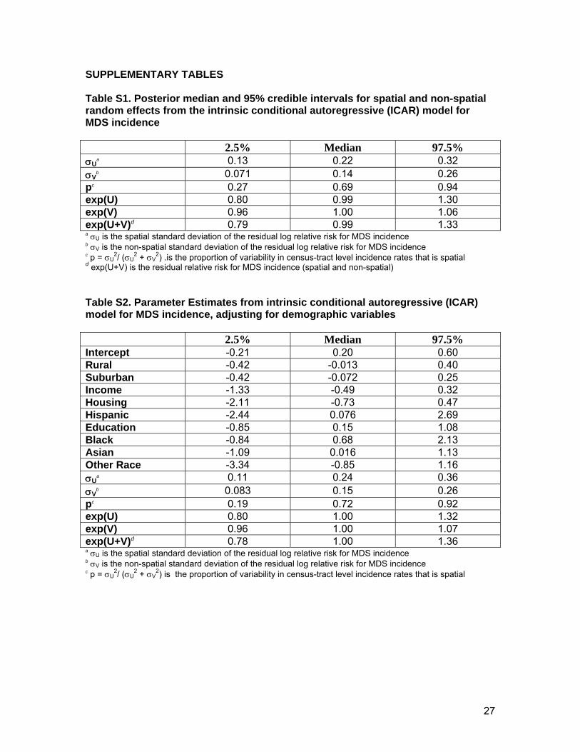
risk is: [0.79, 1.33]). Tables S1 and S2 in the supplementary material contain summaries of the

residual relative risk estimates, total residual variability, and the decomposition into non-spatial

and spatial components – both before and after the inclusion of census-tract-level demographic

covariates in the model. The proportion of the total variability in MDS incidence that is spatial in

nature was estimated to be 69% in unadjusted analyses using the disease mapping approach.

The 95% interval for the census-tract-level spatial residual relative risk for MDS incidence was

(0.80, 1.30), which is larger than the corresponding interval for the non-spatial residual relative

risk (0.96, 1.06). This indicates greater spatial variability than non-spatial variability in relative

risks for MDS incidence; however, the magnitude of the tract-level increases in MDS incidence

are generally not large (e.g., a residual relative risk of 1.30 indicates 30% increased MDS

incidence in a particular tract). The proportion of the total variability in MDS incidence that was

estimated to be spatial in nature increased slightly, to 72%, after inclusion of the demographic

covariates. There was no evidence that any of the covariates was associated with census-tract

level MDS incidence, as evidenced by inclusion of 1 in the 95% intervals for the relative risks,

exp( )β ,associated with the covariates.

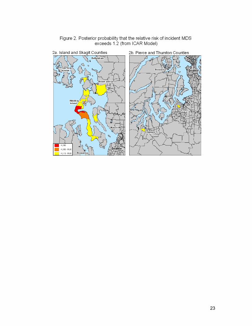
There were 13 census tracts with posterior probabilities greater than 0.70 for relative risk

of MDS incidence exceeding 1.2; these areas were located in Island, Pierce, Skagit, and

Thurston Counties. The identified areas were essentially unchanged in the analysis that

12

adjusted for the demographic covariates. Figure 2a focuses on the census tracts with the

highest posterior probabilities for relative risks exceeding 1.2 (based on the unadjusted

analysis). The census tract with the highest posterior probability (pp=0.96) was located on

Whidbey Island in Island County, with an estimated relative risk of 2.12. Several other identified

tracts were also located on Whidbey Island, as well as in nearby Skagit County. Other identified

areas, shown in Figure 2b, are a census tract located in Tacoma in Pierce County (RR=1.45,

pp=0.79) and a tract in Olympia, Thurston County (RR=1.41, pp=0.71).

There were 13 unique (although sometimes overlapping) clusters of incident MDS (p <

0.005) identified using the Besag and Newell method with k=10 cases. These were located in

Island, Pierce and Thurston counties. With this significance level, we would expect to see 4

clusters due to random chance; hence, there were more clusters than expected. The cluster

locations identified using the Besag and Newell method are displayed in Figure 3a; note that

where clusters overlap, the cluster with the lowest p-value is displayed. The potential cluster

with the lowest p-value (p=0.0006), included two census tracts on Whidbey Island in Island

County. Figure 3b shows the identified cluster locations in Pierce (in and near Tacoma) and

Thurston Counties (Olympia).

The most likely cluster of MDS identified using the spatial scan statistic included 106

cases and encompassed 47 census tracts located in Island, Skagit, Snohomish, San Juan, and

Whatcom Counties; however, this “cluster” was not significant at conventional levels (p = 0.062;

not shown in figures).

First primary MDS

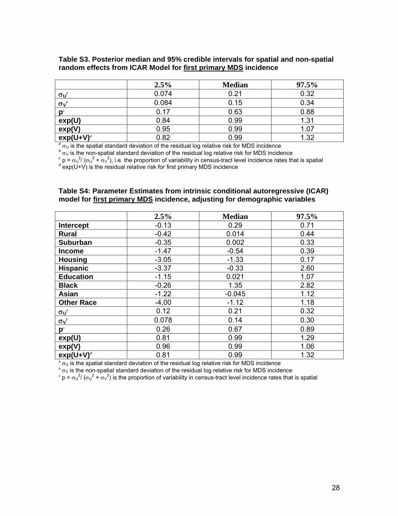
As with all MDS, there was not a great deal of residual variability in relative risk

estimates for first primary MDS incidence (a 95% interval for the residual relative risk is [0.82,

1.32]) in spatial modeling using the disease mapping (ICAR) approach. The proportion of the

total variability that is spatial in nature was estimated to be 63% in the unadjusted analysis, and

13

67% in the analysis adjusting for census-tract-level demographic covariates (supplementary

tables S3 and S4). A 95% interval for the spatial residual relative risks for first primary MDS

incidence is (0.84, 1.31), which is larger than the corresponding interval for non-spatial residual

relative risks (0.95, 1.07). None of the demographic covariates was statistically significantly

associated with census-tract-level incidence rates of first primary MDS.

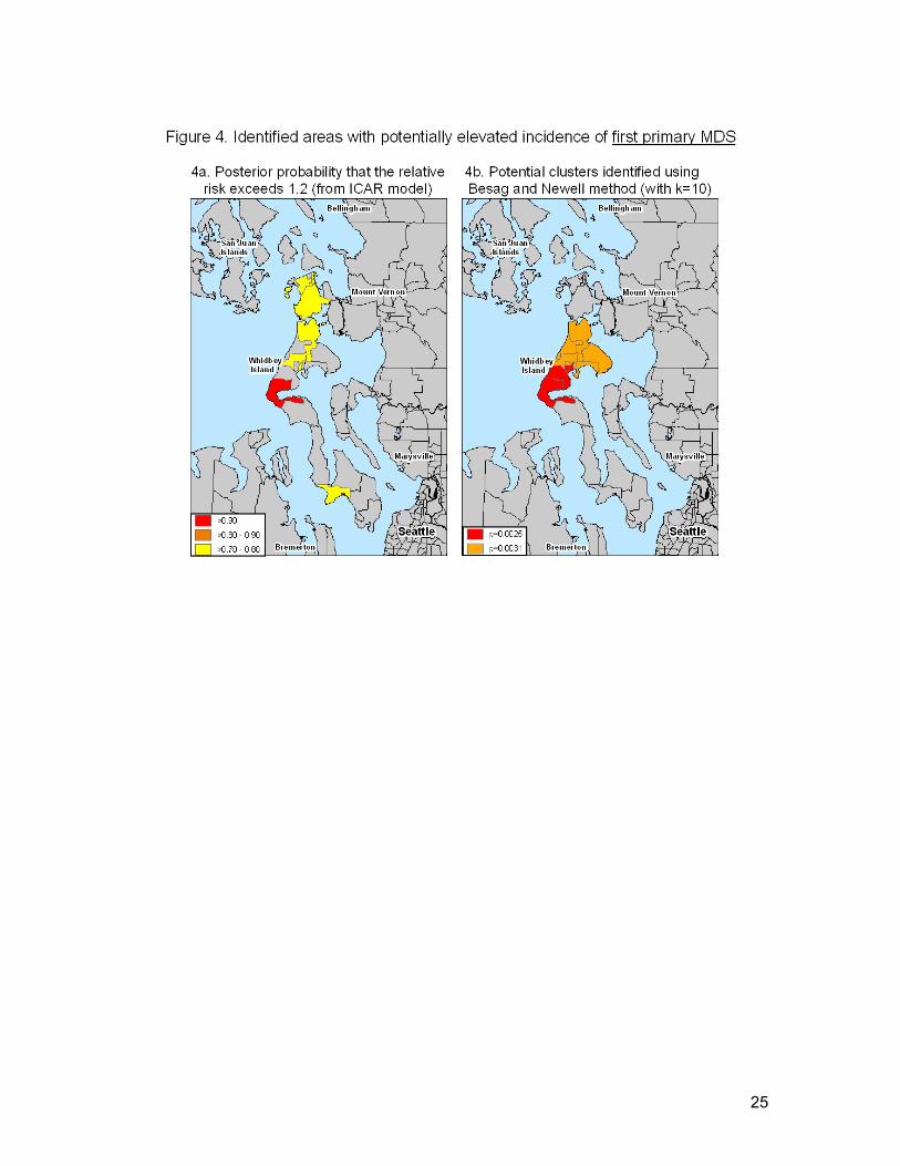
There were 9 census tracts with posterior probabilities greater than 0.70 for relative risks

exceeding 1.2 in unadjusted analyses of first primary MDS, and they were located in Island and

Skagit Counties (Figure 4a). The census tract with the highest posterior probability (pp=0.94)

for an estimated relative risk exceeding 1.2 was the same tract on Whidbey Island in Island

County as that identified for all MDS, and had an estimated relative risk of 2.13.

There were 10 unique (although sometimes overlapping) clusters of first primary MDS

with a significance level of 0.5% identified using the Besag and Newell method with k=10 cases,

which were located in Island, King, and Pierce Counties. As for all MDS, there was a slightly

greater number of clusters detected for first primary MDS than would be expected due to

random chance. The cluster of incident first primary MDS with the lowest p-value (p=0.003) is

shown in Figure 4b, in addition to an overlapping potential cluster. Not shown are two identified

potential clusters in Tacoma, Pierce County (p=0.0034) and near Kent in King County

(p=0.004).

The most likely cluster of first primary MDS identified using a spatial scan statistic

included 67 cases and 39 census tracts located in Island, Skagit, and Snohomish counties (not

shown in figures). This “cluster” was not statistically significant at conventional levels (p =

0.091).

Summary of results across different methods and by definition of MDS

Table 2 shows a summary of results for the disease mapping (ICAR), Besag and Newell,

and Kulldorff methods by definition of MDS. Census tracts on Whidbey Island in Island County

14

were identified as having potentially elevated incidence of all MDS using each of the three

methods, either as individual tracts or contained within a larger cluster including multiple tracts

(Kulldorff method). Essentially the same areas were identified with increased incidence when

restricting to first primary MDS; however, the elevations were not observed in post hoc analyses

restricted to MDS following a previous cancer. MDS incidence was elevated in a census tract in

Tacoma, Pierce County in both the disease mapping (ICAR) and Besag and Newell analyses.

This same census tract in Tacoma was not elevated in analyses restricted to first primary MDS,

but was identified when restricting analyses to MDS following a previous cancer (either

individually or contained within a larger cluster). The Besag and Newell analysis also identified

a second cluster of all MDS in Pierce County, in the Parkland area (suburb of Tacoma), which

included four census tracts. This cluster was adjacent to a potential cluster of first primary MDS

identified using the Besag and Newell method. Areas of potentially elevated incidence in

Olympia, Thurston County were identified for all MDS in the ICAR and Besag and Newell

analyses; these areas were not elevated for first primary MDS but were elevated for MDS

following a previous cancer. The only cluster identified in King County was of first primary MDS,

identified using the Besag and Newell method. This cluster was located south of the city of

Seattle near Kent, Washington.

DISCUSSION

Our analyses did not indicate strong spatial dependence (clustering) either among all MDS

cases or among first primary MDS, as reflected by the relatively narrow 95% intervals for the

estimated census-tract-specific spatial residual relative risks for MDS incidence. Despite little

evidence of overall spatial dependence of MDS incidence across the study region, there was

evidence for specific areas of elevated incidence (clusters). In all three statistical methods, the

highlighted areas tended to overlap. All three methods identified the most likely clusters of all

MDS and first primary MDS in (or including) Whidbey Island in Island County. Significant

15

clusters were also identified in Skagit, Pierce, Thurston, and King Counties. These results

suggest that there may be localized regional environmental exposures causing increased

incidence of MDS, though studies such as these are always subject to drawbacks that make

interpretation difficult, as we detail shortly

We used three methods to identify localized areas with elevated incidence rates, since

each has the ability to detect clusters of different types. For example, the Besag and Newell

method may detect clusters in sparsely populated areas since the population subgroups tested

are selected based on the number of cases, rather than the size of the underlying population (as

in the Kulldorff spatial scan statistic method). For this reason, the spatial scan statistic method

tends to detect larger clusters than Besag and Newell. However, the Kulldorff spatial scan

statistic method more effectively adjusts for multiplicity and dependence of tests than the Besag

and Newell method, generally leading to detection of fewer false clusters, though the inability to

formally assess secondary clusters is a drawback. A major difficulty with both the Besag and

Newell, and the Kulldorff methods is the difficulty in specifying a threshold for deciding upon

whether a p-value is significant. Ideally, a threshold would be dependent on the power (and in

particular on the sizes the expected numbers), but no guidelines are available. A solution for

the method is to simply view the p-values as a means by which regions may be ranked.

The disease mapping (ICAR) model provides more reliable estimates of disease excesses, by

reducing the variance of the estimates through shrinkage towards global- and local averages.

However, such shrinkage can result in missing “high” extremes in disease incidence, since the

extremes tend to undergo the most shrinkage, particularly when the underlying population in

sparse. The specific census tracts on Whidbey Island in Island County that were identified as

having higher-than-expected MDS incidence using both the disease mapping (ICAR) and Besag

and Newell approaches were not specifically singled out using the spatial scan statistic

(Kulldorff method); rather, a 47-tract region inclusive of Whidbey Island was identified as the

16

most likely cluster of MDS (p=0.06). The different results between these approaches may be

due to the relative sparseness of underlying populations in the identified census tracts.

Our study was not designed to identify causal agents, and can only identify geographic

regions for future research of potential causes of MDS. Whidbey Island, where clusters of MDS

and first primary MDS (but not MDS following a previous cancer) were identified, is a relatively

rural, sparsely-populated area of the Seattle-Puget Sound region. Whidbey Island Naval Air

Station is a major employer on the island, and the economy of the island also relies on tourism,

small-scale agriculture, and the arts. Tacoma, Pierce County, is an urban port city, and the

identified regions of elevated MDS incidence in both the ICAR and Besag and Newell methods

are located near the manufacturing/industrial center of the city. In addition to the port, major

industries in the area include paper manufacturing and oil refining. While spatial clusters may

indicate localized environmental causes of MDS, it is also possible that such clusters could arise

due to localized patterns of occupational exposures (e.g., a large industry employer in the area),

lifestyle practices (e.g., higher rates of smoking in the area), or other factors that we could not

adjust for in our investigation. It would be important for future research to obtain individual-level

information on these different types of potential risk factors.

Cancer cluster investigations such as the one presented here are limited when the

case’s location is based on the residential location at the time of diagnosis. This location may

be more or less important for MDS etiology depending on the person’s length of residence in the

home at the time of diagnosis, because long-term exposures or exposures in the distant past

may be more relevant than recent exposure to development of MDS or other cancers.

Nevertheless, the relevant timing of exposure is likely to differ by the specific exposure (e.g., the

type of chemical, physical, or infectious agent). The relevant timing of exposure may also differ

based on previous exposures; for example, recent environmental exposures could

hypothetically be important for MDS following a previous cancer, if previous

chemotherapy/radiation treatment has increased the person’s susceptibility to develop MDS

17

from late-stage carcinogens. Our approach, using residential location at the time of diagnosis

for cases diagnosed from 2002 through 2006 is most appropriate for identifying clusters caused

by a relatively constant exposure that was present in the region during the entire study period

and which acts etiologically in the late stages of carcinogenesis for MDS – for example, during

the year or two before diagnosis. Our approach is less likely to capture clusters due to transient

exposures (e.g., an infectious disease epidemic lasting <1 year) or exposures that act early in

the etiology of MDS (e.g., with a long latency time), due to the limitations of the residential data.

An ideal approach for identifying clusters would be to obtain lifetime residential histories from

MDS cases and a control group. With this type of data, spatial clustering of cases can be

evaluated for specific calendar time periods during which a transient exposure may have

occurred (e.g., multiple cases lived in a local area during the same calendar year), as well as for

time periods defined to account for expected latency of exposure effects (e.g., limiting potential

clustering to residential locations in which the person lived at least 10 years before diagnosis).

The distribution of MDS cases in the Seattle-Puget Sound region likely reflects

underreporting by some local hospitals and more complete reporting by others. However, active

case finding methods employed by the SEER Cancer Surveillance System in Seattle-Puget

Sound are likely to partially resolve localized discrepancies in reporting. Active case-finding

methods include searching hospital disease index codes (ICD-9 codes), pathology reports,

cytogenetics test results, and death certificates in order to find potential cases. Nevertheless, it

is also possible that under certain circumstances MDS would not be detected even with active

case finding. For example, patients who are diagnosed outside of a hospital setting and are not

treated are likely to be missed, as are patients who do not receive definitive diagnostic testing

(i.e., bone marrow biopsy). Incomplete ascertainment of MDS would affect the results of our

spatial analysis of incident MDS if the ‘selection’ of MDS cases into the study population was

differential according to local geographic area. Hypothetically, if MDS cases were

underreported in all other areas outside of Island County, then our results would be spurious;

18

however, this is not a likely scenario given the active case finding methods applied to the entire

region.

MDS comprises a heterogeneous group of histologies, for which risk factors may differ.

A large proportion (35.3%) of the MDS cases in the Seattle-Puget Sound region from 2002-2005

were recorded as MDS, NOS (ICD-O-3 9989). Although cluster investigation for specific MDS

histologic subtypes would be of interest for honing in on the nature of any increased disease

risk, the high proportion of cases in our study with the MDS, NOS subtype raises concerns

about the validity of the ICD-O-3 classification of these cases and therefore limits any

investigation of similarities or differences between MDS subtypes in spatial clustering. Future

studies of MDS in the Seattle-Puget Sound region would benefit from a centralized review of

MDS case pathology.

Despite the limitations of the SEER data, this resource has allowed us to conduct a

spatial analysis in order to identify local regions of interest for future investigation of

environmental or infectious agents as risk factors for MDS in the Seattle-Puget Sound region of

Washington State. Our findings indicate the most likely areas of increased MDS incidence and

first primary MDS incidence located in Island County, and additional potential clusters in Skagit,

Pierce, Thurston, and King Counties. As noted above, our methods are limited based on the

lack of complete residential histories. Nevertheless, inclusion of identified cluster regions in

future population-based research and investigation of individual-level exposures within those

regions could potentially shed light on environmental risk factors for MDS.

19

REFERENCES

1. Schumacher HR, Nand S. Myelodysplastic Syndromes: Approach to Diagnosis and

Treatment. New York: IGAKU-SHOIN Medical Publishers, 1995.

2. Raza A, Mundle SD. Myelodysplastic Syndromes & Secondary Acute Myelogenous

Leukemia: Directions for the New Millennium. Boston: Kluwer Academic Publishers, 2001.

3. Detailed Guide: Myelodysplastic Syndrome. What Are the Key Statistics About

Myelodysplastic Syndromes? American Cancer Society . 2-16-2005 4-11-2005.

4. Lynge E, Anttila A, Hemminki K (1997) Organic solvents and cancer. Cancer Causes

Control 8:406-419.

5. Rollison DE, Howlader N, Smith MT et al. (2008) Epidemiology of myelodysplastic

syndromes and chronic myeloproliferative disorders in the United States, 2001-2004,

using data from the NAACCR and SEER programs. Blood 112:45-52.

6. Surveillance, Epidemiology, and End Results (SEER) Program (www.seer.cancer.gov)

SEER*Stat Database: Incidence - SEER 17 Regs Public-Use, Nov 2005 Sub (2000-2003)

- Linked To County Attributes - Total U.S., 1969-2003 Counties, National Cancer Institute,

DCCPS, Surveillance Research Program, Cancer Statistics Branch, released April 2006,

based on the November 2005 submission.

7. Ma X, Selvin S, Raza A, Foti K, Mayne ST (2007) Clustering in the incidence of

myelodysplastic syndromes. Leuk Res 31:1683-1686.

20

8. International Classification of Diseases for Oncology, 3rd Edition. Fritz A, Percy C, Jack A,

Shanmugaratnam K, Sobin L, Parkin DM, Whelan S, editors. 2000 Geneva, World Health

Organization.

9. US Census Bureau. Census 2000 Summary File 1 - Washington State.

http://www2.census.gov/census_2000/datasets/Summary_File_1/Washington/ . 2002

Washington, DC.

10. Spiegelhalter DJ, Thomas A, Best NG. WinBUGS User Manual, version 1.1.1. Cambridge:

1998.

11. Wakefield J (2007) Disease mapping and spatial regression with count data. Biostatistics

8:158-183.

12. Besag J, Newell J (1991) The Detection of Clusters in Rare Diseases. Journal of the Royal

Statistical Society Series A-Statistics in Society 154:143-155.

13. Kulldorff M. A spatial scan statistic. Communications in Statistics: Theory and Methods 26,

1481-1496. 1997

21

Table 1. Characteristics of MDS cases included in the investigation of spatial clustering in the Seattle-Puget Sound region of Washington Statea MDS Casesb

N (%) 2000 Census Population

N (%) Total 1225 4,045,707 Age (years) <50 63 (5.1) 2,991,622 (73.9) 50-59 111 (9.1) 470,017 (11.6) 60-69 178 (14.5) 259,535 (6.4) 70-79 394 (32.2) 203,610 (5.0) 80-84 256 (20.9) 65,417 (1.6) ≥85 223 (18.2) 55,506 (1.4) Sex Female 543 (44.3) 2,030,879 (50.2) Male 682 (55.7) 2,014,828 (49.9) Race White 1114 (90.9) 3,253,688 (80.4) Non-white or unknown 111 (9.1) 792,019 (19.6) Year of diagnosis 2002 230 (18.8) - 2003 234 (19.1) - 2004 258 (21.1) - 2005 255 (20.8) - 2006 248 (20.2) - Previous cancer diagnosis No (first primary MDS) 863 (70.4) - Yes 362 (29.6) - a Study area included 13 counties and 887 census tracts in Washington State that report to the Cancer Surveillance System of the Surveillance, Epidemiology, and End Results (SEER) program b 13 of the total 1238 MDS cases were excluded from analyses due to missing information on residential location

22

23

24

25

26

Table 2. Western Washington Counties identified as having census tracts with increased MDS incidence* All MDS

(N=1225) First primary MDS (n=863)

MDS following a previous cancer (n=362)

Disease mapping (ICAR) (posterior probability >0.70 that RR>1.2 for any specific tract)

Island (Whidbey) (pp=0.96, RR=2.12) Pierce (Tacoma) Skagit Thurston (Olympia)

Island (Whidbey) (pp=0.94, RR=2.13) Skagit

San Juan (pp=0.76, RR=2.02) Pierce (Tacoma)

Besag and Newell (k=10) (clusters w/ p<0.005)

Island (Whidbey) (p=0.0006) Thurston (Olympia) Pierce (Tacoma, Parkland)

Island (Whidbey) (p=0.0025) King (Kent) Pierce (Parkland)

Pierce (Tacoma) (p=0.00017) Thurston (Olympia) King (Kent)

Kulldorff scan statistic (most likely cluster)

Island, Skagit, Snohomish, San Juan, and Whatcom (includes 106 cases, 47 tracts, p=0.062)

Island, Skagit, and Snohomish (includes 67 cases, 39 tracts, p=0.092)

Grays Harbor, Mason, Pierce, and Thurston (includes 101 cases, 167 tracts, p=0.215)

*Counties listed within each table cell are ordered based on the importance of the identified clusters within the county, with the most significant on top to least significant on bottom.

27

SUPPLEMENTARY TABLES

Table S1. Posterior median and 95% credible intervals for spatial and non-spatial random effects from the intrinsic conditional autoregressive (ICAR) model for MDS incidence 2.5% Median 97.5% σU

a 0.13 0.22 0.32 σV

b 0.071 0.14 0.26 pc 0.27 0.69 0.94 exp(U) 0.80 0.99 1.30 exp(V) 0.96 1.00 1.06 exp(U+V)d 0.79 0.99 1.33 a σU is the spatial standard deviation of the residual log relative risk for MDS incidence b σV is the non-spatial standard deviation of the residual log relative risk for MDS incidence c p = σU

2/ (σU2 + σV

2) .is the proportion of variability in census-tract level incidence rates that is spatial d exp(U+V) is the residual relative risk for MDS incidence (spatial and non-spatial) Table S2. Parameter Estimates from intrinsic conditional autoregressive (ICAR) model for MDS incidence, adjusting for demographic variables 2.5% Median 97.5% Intercept -0.21 0.20 0.60 Rural -0.42 -0.013 0.40 Suburban -0.42 -0.072 0.25 Income -1.33 -0.49 0.32 Housing -2.11 -0.73 0.47 Hispanic -2.44 0.076 2.69 Education -0.85 0.15 1.08 Black -0.84 0.68 2.13 Asian -1.09 0.016 1.13 Other Race -3.34 -0.85 1.16 σU

a 0.11 0.24 0.36 σV


2/ (σU2 + σV

2) is the proportion of variability in census-tract level incidence rates that is spatial

28

Table S3. Posterior median and 95% credible intervals for spatial and non-spatial random effects from ICAR Model for first primary MDS incidence 2.5% Median 97.5% σU

a 0.074 0.21 0.32 σV


2/ (σU2 + σV

2), i.e. the proportion of variability in census-tract level incidence rates that is spatial d exp(U+V) is the residual relative risk for first primary MDS incidence Table S4: Parameter Estimates from intrinsic conditional autoregressive (ICAR) model for first primary MDS incidence, adjusting for demographic variables 2.5% Median 97.5% Intercept -0.13 0.29 0.71 Rural -0.42 0.014 0.44 Suburban -0.35 0.002 0.33 Income -1.47 -0.54 0.39 Housing -3.05 -1.33 0.17 Hispanic -3.37 -0.33 2.60 Education -1.15 0.021 1.07 Black -0.26 1.35 2.82 Asian -1.22 -0.045 1.12 Other Race -4.00 -1.12 1.18 σU

a 0.12 0.21 0.32 σV


2/ (σU2 + σV

2) is the proportion of variability in census-tract level incidence rates that is spatial

Documents

Spatial Clustering of Myelodysplastic Syndromes (MDS) in ...authors.fhcrc.org/445/1/DeRoosACCCManuscript080610.pdfSpatial Clustering of Myelodysplastic Syndromes (MDS) in the Seattle-Puget