1

Spatial Autocorrelation

Daniel A. Griffith

Department of Geography, Syracuse University

_____________________________________________________________________________

I. Introduction

II. Definition of Notation

III. Conceptual Meanings of Spatial Autocorrelation

IV. Estimators of Spatial Autocorrelation

V. Theoretical Statistical Properties of Spatial Autocorrelation

VI. Common Probability Model Specifications with Spatial Autocorrelation

VII. What Should an Applied Spatial Scientist Do?

_____________________________________________________________________________

Glossary

auto- model A statistical model whose associated probability density/mass function contains a

linear combination of the dependent variable values at nearby locations.

correlation A description of the nature and degree of a relationship between a pair of

quantitative variables.

covariance matrix A square matrix whose diagonal entries are the variances of, and whose off-

diagonal entries are the covariances between, the row/column labeling variables.

estimator A statistic calculated from data to estimate the value of a parameter.

geographic connectivity/weights matrix An n-by-n matrix with the same sequence of row and

column location labels, whose entries indicate which pairs of locations are neighbors.

geostatistics A set of statistical tools used to exploit spatial autocorrelation contained in

georeferenced data usually for spatial prediction purposes.

2

Moran scatterplot A scatterplot of standardized versus summed nearby standardized values

whose associated bivariate regression slope coefficient is the unstandardized Moran Coefficient.

semivariogram plot A scatterplot of second-order spatial dependence exhibited in

georeferenced data.

spatial autoregression A set of statistical tools used to accommodate spatial dependency effects

in conventional linear statistical models.

spatial statistics A more recent addition to the statistics literature that includes geostatistics,

spatial autoregression, point pattern analysis, centrographic measures, and image analysis.

_____________________________________________________________________________

Spatial autocorrelation is the correlation among values of a single variable strictly attributable

to their relatively close locational positions on a two-dimensional surface, introducing a

deviation from the independent observations assumption of classical statistics.

I. Introduction

Social scientists often study the form, direction and strength of the relationship exhibited by two

quantitative variables measured for a single set of n observations. A scatterplot visualizes this

relationship, with a conventional correlation coefficient describing the direction and strength of a

straight-line relationship of the overall pattern. A variant of conventional correlation is serial

correlation, which pertains to the correlation between values for observations of a single variable

according to some ordering of these values. Its geographic version is spatial autocorrelation (auto

meaning self), the relationship between a value of some variable at one location in space and

nearby values of the same variable. These neighboring values can be identified by an n-by-n

binary geographic connectivity/weights matrix, say, C; if two locations are neighbors, then cij =

1, and if not, then cij = 0 (see Figure 1, in which two areal units are deemed neighbors if they

share a common non-zero length boundary).

3

********** FIGURE 1 about here **********

Positive spatial autocorrelation means that geographically nearby values of a variable tend to be

similar on a map: high values tend to be located near high values, medium values near medium

values, and low values near low values. Most social science variables tend to be moderately

positively spatially autocorrelated because of the way phenomena are geographically organized.

Demographic and socio-economic characteristics like population density and house price are

good examples of variables exhibiting positive spatial autocorrelation. Neighborhoods tend to be

clusters of households with similar preferences. Families tend to organize themselves in a way

that concentrates similar household attributes on a map—creating positive spatial autocorrelation

amongst many variables—with government policies and activities, such as city planning and

zoning, reinforcing such patterns.

A. Why measure and account for spatial autocorrelation?

Spatial analysis frequently employs model-based statistical inference, the dependability of which

is based upon the correctness of posited assumptions about a model's error term. One principal

assumption states that individual error terms come from a population whose entries are

thoroughly mixed through randomness. Moreover, the probability of a value taken on by one of a

model's error term entries does not affect the probability of a value taken on by any of the

remaining error term entries (i.e., the independent observations assumed in classical statistics).

Non-zero spatial autocorrelation in georeferenced data violates this assumption and is partly

responsible for geography existing as a discipline. Without it few variables would exhibit a

geographic expression when mapped; with it most variables exhibit some type of spatial

organization across space. Zero spatial autocorrelation means geographically random phenomena

and chaotic landscapes!

4

Therefore, there are two primary reasons to measure spatial autocorrelation. First, it indexes the

nature and degree to which a fundamental statistical assumption is violated, and, in turn,

indicates the extent to which conventional statistical inferences are compromised when non-zero

spatial autocorrelation is overlooked. Autocorrelation complicates statistical analysis by altering

the variance of variables, changing the probabilities that statisticians commonly attach to making

incorrect statistical decisions (e.g., positive spatial autocorrelation results in an increased

tendency to reject the null hypothesis when it is true). It signifies the presence of and quantifies

the extent of redundant information in georeferenced data, which in turn affects the information

contribution each georeferenced observation makes to statistics calculated with a database.

Accordingly, more spatially autocorrelated than independent observations are needed in

calculations to attain an equally informative statistic.

Second, the measurement of spatial autocorrelation describes the overall pattern across a

geographic landscape, supporting spatial prediction and allowing detection of striking deviations.

Cressie (1991) notes that in many situations spatial prediction is as important as temporal

prediction/forecasting. He further notes that explicitly accounting for it tends to increase the

percentage of variance explained for the dependent variable of a predictive model and does a

surprisingly good job of compensating for unknown variables missing from a model

specification. Griffith and Layne (1999) report that exploiting it tends to increase the R-squared

value by about 5%, and obtaining 5% additional explanatory power in this way is much easier

and more reliably available than getting it from collecting and cleaning additional data or from

using different statistical methods.

B. Graphical portrayals of spatial autocorrelation

By graphically portraying the relationship between two quantitative variables measured for the

same observation, a scatterplot relates to the numerical value rendered by a correlation

5

coefficient formula. Not surprisingly, then, specialized versions of this scatterplot are closely

associated with measures of spatial autocorrelation.

The Moran scatterplot is one such specialized version. To construct it, first values of the

georeferenced variable under study, say Y, are converted to z-scores, say zY. Next, those adjacent

or nearby z-score values of Y are summed; this can be achieved with the matrix product CZY,

where ZY is the vector concatenation of the individual zY values. Finally, the coordinate pairs

(zY,i, ∑=

n

1jYjijzc ), i=1, 2, …, n, are plotted on the graph whose vertical axis is CZY and whose

horizontal axis is ZY. This construction differs from that proposed by Anselin (1995), who uses

matrix W, the row-standardized stochastic version of matrix C, to define the vertical axis. An

example of this graphic illustrates a case of positive spatial autocorrelation (Figure 1).

Another specialized scatterplot is the semivariogram plot, which is comprehensively described

by Cressie (1991). To construct it, first, for each pair of georeferenced observations both the

distance separating them and the squared difference between their respective attribute values are

calculated. Next, distances are grouped into G compact ranges preferably having at least 30

paired differences, and then group averages of the distances and of the squared attribute

differences are computed. Semivariance values equal these squared attribute differences divided

by 2. Finally, on a graph whose vertical axis is average semivariance and whose horizontal axis

is average distance, the following coordinate pairs are plotted: (∑∑ −δ= =

n

1i

n

1jg

2jiij )K2/()yy( ,

∑∑δ= =

n

1i

n

1jgijij K/d ), where Kg is the number of i-j pairs in group g— ∑

=

G

1ggK = n(n!1)—dij is the

distance separating locations i and j, and δij is a binary 0/1 variable denoting whether or not both

locations i and j belong to group g. The steep slope in Figure 1 indicates very strong positive

autocorrelation that is due, in part, to a geographic trend in the data.

6

C. Autoregressive and geostatistical perspectives on spatial autocorrelation

Treatments of georeferenced data focus on either spatial autocorrelation (addressed in

geostatistics) or partial spatial autocorrelation (addressed in spatial autoregression). The two

classic works reviewing and extending spatial statistical theory are by Cliff and Ord (1981), who

have motivated research involving spatial autoregression, and Cressie (1991), who has

summarized research involving geostatistics. These two subfields have been evolving

autonomously and in parallel, but they are closely linked through issues of spatial interpolation

(e.g., the missing data problem) and of spatial autocorrelation. They differ in that geostatistics

operates on the variance-covariance matrix while spatial autocorrelation operates on the inverse

of this matrix. More superficial differences include foci on more or less continuously occurring

attributes (geostatistics) versus aggregations of phenomena into discrete regions (i.e., areal units)

(spatial autoregression); and, on spatial prediction (geostatistics) versus enhancement of

statistical description and improvement of the inferential basis for statistical decision making

(i.e., increasing precision) (spatial autoregression). Griffith and Layne (1999), among others,

present graphical, numerical and empirical findings that help to articulate links between

geostatistics and spatial autoregression (see § V).

II. Definition of notation

One convention employed here denotes matrices with bold letters; another denotes names by

subscripts. Definitions of notation used throughout appear in Table 1.

********** TABLE 1 about here **********

III. Conceptual meanings of spatial autocorrelation

Spatial autocorrelation can be interpreted in different ways.

As a nuisance parameter spatial autocorrelation is inserted into a model specification because its

presence is necessary for a good description, but it is not of interest and only "gets in the way" of

7

estimating other model parameters. In fact, if the value of this parameter were known, resulting

statistical analyses would be much simpler and more powerful. Nonspatial analysts especially

view spatial autocorrelation as an interference. They study the relationship between two

quantitative variables that happen to be georeferenced, with spatial autocorrelation lurking in the

background. Mean response and standard errors improve when spatial autocorrelation is

accounted for, while conventional statistical theory could be utilized if the value of this

parameter were known or set to 0. Ignoring latent spatial autocorrelation results in increased

uncertainty about whether findings are attributable to assuming zero spatial autocorrelation (i.e.,

misspecification).

As self-correlation spatial autocorrelation is interpreted literally: correlation arises from the

geographic context within which attribute values occur. As such it can be expressed in terms of

the Pearson product moment correlation coefficient formula, but with neighboring values of

variable Y replacing those of X:

∑∑

∑

==

=

−−

−−

n

1i

2i

n

1i

2i

n

1iii

n/)yy(n/)xx(

n/)yy)(xx( becomes

∑∑

∑∑ ∑∑

==

= = = =

−−

−−

n

1i

2i

n

1i

2i

n

1i

n

1j

n

1i

n

1jijjiij

n/)yy(n/)yy(

c/)yy)(yy(c . (1)

The left-hand expression converts to the right-hand one by substituting ys for xs in the right-hand

side, by computing the numerator term only when a 1 appears in matrix C, and by averaging the

numerator cross-product terms over the total number of pairs denoted by a 1 in matrix C. The

denominator of the revised expression (1) is the sample variance of Y, 2Ys . Coupling this with

part of the accompanying numerator term renders Y

jn

1jij

Y

i

s)yy(

cs

)yy( −− ∑=

, where this summation

term is the quantity measured along the vertical axis of the modified Moran scatterplot; the right-

hand part of expression (1) is known as the Moran Coefficient (MC). Accordingly, positive

8

spatial autocorrelation occurs when the scatter of points on the associated Moran scatterplot

reflects a straight line sloping from the lower left-hand to the upper right-hand corner: high

values on the vertical axis tend to correspond with high values on the horizontal axis, medium

values with medium values, and low values with low values (see Figure 1). Negligible spatial

autocorrelation occurs when the scatter of points suggests no pattern: high values on the vertical

axis correspond with high, medium and low values on the horizontal axis, as would medium and

low values on the vertical axis. Negative spatial autocorrelation occurs when the scatter of points

reflects a straight line sloping from the upper left-hand to the lower right-hand corner: high

values on the vertical axis tend to correspond with low values on the horizontal axis, medium

values with medium values, and low values with high values. These patterns are analogous to

those for two different quantitative attribute variables—X and Y—rendering, respectively, a

positive, zero, and negative Pearson product moment correlation coefficient value.

The semivariogram is based upon squared paired comparisons of georeferenced data values.

Emphasizing variation with distance rather than only with nearby values, the numerator of

expression (1) may be replaced by ]c2/[)yy(cn

1i

n

1j

n

1i

n

1jij

2jiij∑∑ ∑∑

= = = =

− , converting this measure to

the Geary Ratio (GR) when the unbiased sample variance is substituted in the denominator.

As map pattern spatial autocorrelation is viewed in terms of trends, gradients or mosaics across a

map. This more general meaning can be obtained by studying the matrix form of the MC,

specifically the term YT(I ! 11T/n)C(I ! 11T/n)Y corresponding to the first summation in

expression(1), where I is an n-by-n identity matrix, 1 is an n-by-1 vector of ones, T is the matrix

transpose operation, and (I ! 11T/n) is the projection matrix commonly found in conventional

multivariate and regression analysis that centers the vector Y. The extreme eigenvalues of matrix

expression (I ! 11T/n)C(I ! 11T/n) determine the range of the modified correlation coefficient,

9

MC; therefore, MC is not restricted to the range [!1, 1]. Furthermore, Tiefelsdorf and Boots

(1995) show that the full set of n eigenvalues of this expression establishes the set of distinct MC

values associated with a map, regardless of attribute values. The accompanying n eigenvectors

represent a kaleidoscope of orthogonal and uncorrelated map patterns of possible spatial

autocorrelation:

The first eigenvector, say E1*, is the set of numerical values that has the largest MC achievable by any

set, for the spatial arrangement defined by the geographic connectivity matrix C. The second eigenvector

is the set of values that has the largest achievable MC by any set that is uncorrelated with E1*. This

sequential construction of eigenvectors continues through En*, which is the set of values that has the

largest negative MC achievable by any set that is uncorrelated with the preceding (n!1) eigenvectors.

As such, Griffith (2000) argues that these eigenvectors furnish distinct map pattern descriptions

of latent spatial autocorrelation in georeferenced variables.

As a diagnostic tool spatial autocorrelation plays a crucial role in model-based inference, which

is built upon valid assumptions rather than upon the outcome of a proper sampling design.

Sometimes spatial autocorrelation is used as a diagnostic tool for model misspecification, being

viewed as an artifact of overlooked nonlinear relationships, nonconstant variance or outliers.

Cliff and Ord (1981) furnish an excellent example with their empirical analysis of the

relationship between percentage change in population and arterial road accessibility across the

counties of Eire. MC = 0.1908 for residuals obtained from a bivariate regression using these two

variables; MC = 0.1301 for residuals obtained from a bivariate regression applying a logarithmic

transformation to each of these two variables. Yet, Griffith and Layne (1999) determine and then

employ an optimal Box-Tidwell linearization transformation for these data, which renders MC =

!0.0554 for the residuals, a value that suggests the absence of spatial autocorrelation. In other

10

words, the weak positive spatial autocorrelation detected by Cliff and Ord is due solely to a

nonlinear model misspecification.

As redundant information spatial autocorrelation represents duplicate information contained in

georeferenced data, linking it to missing values estimation as well as to notions of effective

sample size and degrees of freedom. For normally distributed variables these latter two quantities

establish a correspondence between n spatially autocorrelated and, say, n* zero spatial

autocorrelation (i.e., independent) observations. Richardson and Hémon (1981) promote this

view for correlation coefficients computed for pairs of geographically distributed variables.

Haining (1991) demonstrates an equivalency between their findings and the results obtained by

removing spatial dependency effects with filters analogous to those used in constructing time

series impulse-response functions.

Inference about a geographic variable mean when non-zero spatial autocorrelation is present: is

impacted upon by a variance inflation factor (VIF), and has n* # n. The respective matrix

formulae—where TR denotes the matrix trace operation and Vσ!2 denotes the n-by-n inverse

variance-covariance matrix capturing latent spatial autocorrelation effects—are VIF = TR(V!1)/n

and n* = nHTR(V!1)/ 1V!11. Selected results for these two formulae appear in Table 2, where

ρ̂ SAR denotes estimated spatial autocorrelation using a simultaneous autoregressive (SAR) model

specification (see §IV), and suggest that: on average roughly two-thirds of the information

content is redundant; spatial autocorrelation is at least doubling the variance; and, for example, a

cluster of about 10 additional census tracts needs to be acquired for Houston before as much new

information is obtained as is contained in a single, completely isolated census tract in this

metropolitan region.

********** TABLE 2 about here **********

11

As a missing variables indicator/surrogate spatial autocorrelation accounts for variation

otherwise unaccounted for because of variables missing from a regression equation. This

perspective is particularly popular among spatial econometricians (e.g., Anselin, 1988). In

essence, autocorrelation effects latent in predictor variables match autocorrelation effects in Y.

For instance, one well-known covariate of population density is distance from the central

business district (CBD). For Adair (Table 2), a bivariate regression analysis reveals that this

variable accounts for about 91% of the variation in population density across the county, while

ρ̂ SAR decreases to 0.33686 and the total percentage of variance accounted for increases slightly

to about 92%. (The trend contributes considerably to the nature of the semivariogram plot curve

appearing in Figure 1.) For Chicago, a bivariate regression analysis reveals that this variable

accounts for about 42% of the variation in population density across the city, while ρ̂ SAR

decreases to 0.76994 and the total percentage of variance accounted for remains at roughly 68%.

As a spatial spillover effect spatial autocorrelation results from effects of some phenomenon at

one location "spilling over" to nearby locations, much like a flooding river overflowing its banks.

Pace and Barry (1997) furnish an empirical example of house price spillover: the value of a

house is a function of both its dwelling attributes and the value of surrounding houses. They

study 20,640 California blockgroups having houses, and report ρ̂ SAR = 0.8536, indicating the

presence of strong positive spatial autocorrelation, with inclusion of the autoregressive term

increasing the percentage of variance explained by 25%.

As a spatial process mechanism spatial autocorrelation is viewed as the outcome of some course

of action operating over a geographic landscape. The contagious spread of disease, the

dissemination of information or ideas, and spatial competition illustrate this viewpoint, while an

auto-logistic model (see §VI) describes it: 1 denotes the presence and 0 denotes the absence of

some phenomenon at different locations in a geographic landscape.

12

As an outcome of areal unit demarcation spatial autocorrelation relates to the modifiable areal

unit problem (MAUP), whereby results from statistical analyses of georeferenced data can be

varied at will simply by changing the surface partitioning to demarcate areal units. In an analysis

of variance framework, devising areal units in a way that manipulates attribute differences within

and between them impacts upon the nature and degree of measured spatial autocorrelation. If this

practice is executed in a gerrymandering fashion, a range of possible spatial autocorrelation,

from positive to negative, materializes. In part, accounting for detected spatial autocorrelation in

statistical analyses attempts to neutralize such outcomes.

IV. Estimators of spatial autocorrelation

Spatial autocorrelation may be indexed, quantified by including an autoregressive parameter in a

regression model, or filtered from variables.

Spatial autocorrelation can be quantified with indices. Expression (1) furnishes the MC index,

which also can be rewritten in terms of the regression coefficient affiliated with a Moran

scatterplot. Its range is roughly "1; more precisely, it is [ ∑∑= =

λn

1i

n

1jijmin c/n , ∑∑

= =

λn

1i

n

1jijmax c/n ],

where λmin and λmax are the extreme eigenvalues of matrix (I!11T/n)C(I!11T/n). As MC

approaches this upper limit, the paired values (ZY, CZY) in a Moran scatterplot increasingly

align with a straight line having a positive slope; as MC approaches this lower limit, the

alignment is with a straight line having a negative slope. As MC approaches !1/(n!1) (its

expected value indicating zero spatial autocorrelation) the paired values should resemble a

random scatter of points. The standard error of this statistic is approximately ∑∑= =

n

1i

n

1jijc/2 ; in

terms of practical importance, modest levels of positive spatial autocorrelation begin at

13

0.5MC/MCmax, whereas moderate levels begin at 0.7MC/MCmax, and substantial levels begin at

0.9MC/MCmax.

One variation of this index is the GR, which replaces the numerator of expression (1) with a

squared paired comparison and the denominator with the unbiased sample variance estimate.

This index roughly ranges from 0 (i.e., yi = yj), indicating perfect positive spatial autocorrelation,

to 2, strong negative spatial autocorrelation; now 1 indicates zero spatial autocorrelation. GR is

inversely related to MC. The extreme values are more precisely given by

[ ∑∑= =

−λ−n

1i

n

1jij1n c/)1n( , ∑∑

= =

λ−n

1i

n

1jijmax c/)1n( ], where λn!1 and λmax are the second smallest and the

largest eigenvalues of matrix (<1TC>diagonal ! C), where <1TC>diagonal is a diagonal matrix whose

diagonal entries are the row sums of C. This feature highlights that GR emphasizes edges and

numbers of neighbors far more than MC does.

Another variation is the triplet of join count statistics used to analyze 0/1 binary georeferenced

data, conveniently coded as 1 denoting black (B) and 0 denoting white (W). The number of

neighboring pairs of 1s on a map equals 2BB, the number of neighboring pairs of 0s equals

2WW, and the number of 1s with neighboring 0s equals 2BW; BB + BW + WW = ∑∑= =

n

1i

n

1jijc /2,

where n1 is the number of 1s. These quantities can be interpreted in terms of binomial random

variables. The numerator of the MC reduces to ∑∑= =

n

1i

n

1jij

21 cn /n2 + 2(1!n1/n)BB ! 2(n1/n)BW.

Spatial autocorrelation can be quantified by including an autoregressive parameter in a model

specification. Regression becomes autoregression, as is demonstrated by Griffith and Layne

(1999), with the most common specifications being the SAR (Y = ρSARWY + (I ! ρSARWY)Xß +

ε), the AR (Y = ρARWY + Xß + ε), and the CAR (Y = Xß + (I!ρARC)!1/2ε) model, where ß is a

vector of regression coefficients and ε is a vector of independent and identically distributed

14

random error terms. These are popular among spatial statisticians, spatial econometricians and

image analysts, respectively. The SAR model specifies spatial autocorrelation as being in the

error term, with the attribute error at location i being a function of the average of nearby error

values: E(Y) = Xß, VAR(Y) = σ2[(I ! ρSARWT)(I ! ρSARW)]!1, where E denotes the calculus of

expectation operator. The AR model specifies spatial autocorrelation as being a direct

dependency among the Y values: E(Y) = (I ! ρARW)!1Xß, VAR(Y) = σ2[(I ! ρARWT)(I !

ρARW)]!1. The CAR model specifies spatial autocorrelation as being in the error term, with a

weaker degree and smaller spatial field than the SAR model, and with the attribute error at

location i being a function of the sum of nearby error values: E(Y) = Xß, VAR(Y) = σ2(I !

ρCARC)!1. Parameters of these models must be estimated using maximum likelihood techniques.

Parameterizing spatial autocorrelation through the semivariogram plot involves modeling the

relationship between semivariance, γ, and distance, d. Dozens of specifications—most of which

are inventoried in Cressie (1991) and Griffith and Layne (1999)—may be employed, all

describing spatial autocorrelation as a nonlinear decreasing function of distance. The most

popular ones are the spherical, the exponential and the Gaussian; one that should grow in

popularity is the Bessel function. The empirical semivariogram in Figure 1 is best described by a

Bessel function, K1, both before and after adjusting for the underlying distance decay trend. Each

semivariogram model describes the decline in spatial autocorrelation with increasing distance in

terms of an intercept (nugget), a slope, and an implicit/explicit range of spatial dependency. For

Adair County population density (Figure 1), γ̂ = 0.13 + 14.07[1 ! (d/0.25)K1(d/0.25)].

Summarizing the variance-covariance matrix with this type of equation allows new variance-

covariance matrices to be constructed for locations whose attribute values are unknown,

permitting sensible predictions of their values.

15

Spatial filters remove spatial autocorrelation from variables by casting it as redundant

information or as an outcome of map pattern. This former interpretation is employed by Haining

(1991) and renders a spatial linear operator filter (I ! ρ̂ SARW); this latter interpretation renders

predictor variables, such as the battery of eigenvectors Ej*, that capture locational information

summarized by a spatial autocorrelation parameter like ρ̂ SAR. Of note is that Getis (1990)

suggests an alternative form of these spatial filters. For Adair County (Figure 1), the correlation

between log-distance and log-density is !0.936; the spatial linear operator filter results based on

an SAR model ( ρ̂ SAR = 0.95298; Table 2) are !0.985. Eigenfunction filtering identifies two

eigenvectors (MC = 0.76 and 0.47) that account for the residual spatial autocorrelation and

increase the variance accounted for in log-population density by about 4%.

V. Theoretical statistical properties of spatial autocorrelation

Classical statistics establishes the quality of parameter estimators with specific properties that

discriminate between useful and useless ones. Four of these properties are described here.

An unbiased estimator's sampling distribution arithmetic mean equals its corresponding

population parameter value. This property is evaluated with the calculus of expectations. In

general, in the presence of non-zero spatial autocorrelation conventional estimators for first-order

moments are unbiased while those for second-order moments are biased. For example, for linear

regression, E(Y) = E(Xß + V!1/2εσ) = Xß. Similarly, E(b) = E[(XTX)!1XY] = ß, where b is the

ordinary least squares (OLS) regression coefficients estimator. But, E[(Y ! Xß)T(Y ! Xß)/n] =

σ2TR(V)/n, which reduces to σ2 only when V = I. Griffith and Lagona (1998) report that

misspecifying matrix C, of which matrix V is a function, results in b remaining unbiased and s2

remaining biased when autocorrelation is accounted for.

An efficiency estimator is an unbiased estimator whose sampling distribution has the smallest

possible variance, maximizing its reliability. Cordy and Griffith (1993) find that in the presence

16

of non-zero spatial autocorrelation, the biased OLS variance estimator negates much of its

computational simplicity advantage. Consequently, the OLS standard error estimator tends to

underestimate the true standard error when positive spatial autocorrelation prevails. By

accounting for latent spatial autocorrelation, gains in efficiency increase as both its magnitude

and n increase. With regard to the aforementioned VIF and n*: E[( y ! µY)2] = (1TV!11/n)(σ2/n);

and, E[(Y ! µY1)T(Y ! µY1)/n] = [TR(V!1)](σ2/n). These results reduce to their respective

standard results of σ2/n and σ2 only when V = I. A measure of OLS efficiency when spatial

autocorrelation is non-zero is given by n2/[1TV!111TV1]; when spatial autocorrelation is zero,

this quantity equals 1, whereas when perfect positive spatial autocorrelation exists, it is 0.

Griffith and Lagona (1998) report that misspecifying matrix C results in b being asymptotically

efficient and s2 remaining inefficient when autocorrelation is accounted for.

A consistent estimator's sampling distribution concentrates at the corresponding parameter value

as n increases. Considering situations in which the maximum number of neighbors for any given

location is finite: when sample size increases by increasing the size of a region to an unbounded

surface (i.e., increasing domain asymptotics), consistency of the mean and variance estimators is

attained; when sample size increases by partitioning a region into an increasingly finer

tessellation (i.e., infill asymptotics), consistency is lost. Griffith and Lagona (1998) report that

misspecifying matrix C in a typical situation results in b and s2 being consistent, with the

autocorrelation parameter failing to converge to its true value.

A sufficient estimator utilizes all of the pertinent information content of a sample needed to

estimate a particular parameter. This property is established using the factorization criterion for a

likelihood function. A likelihood can be rewritten as the product of a term that depends on the

sample only through the value of the parameter estimator and of a term independent of the

corresponding parameter. The importance of this property is twofold: (1) estimating missing

17

georeferenced data requires imputation of the complete-data sufficient statistics, which in the

case of an auto-normal probability model involves a spatial autocorrelation term; and, (2) the

Markov Chain Monte Carlo (MCMC) procedure used to estimate the auto-logistic and auto-

binomial models requires the sufficient statistics, again one being a spatial autocorrelation term.

VI. Common auto- probability model specifications

The normal distribution is the base of much statistical analysis of continuous data. The binomial

distribution plays the same role for binary variables and percentages, while the Poisson

distribution plays the same role for counts. Auto- specifications of these models almost always

have pairwise-only spatial dependence.

The auto-Gaussian model specification yields the likelihood function

L = constant ! (n/2)LN(σ2) + (1/2)LN[det(V!1)] ! (Y!Xß)TV(Y!Xß)/(2 σ2) ,

where LN denotes the natural logarithm, and det denotes the matrix determinant operation. The

normalizing constant, (1/2)LN[det(V!1)], complicates calculation of the maximum likelihood

estimates of parameters because it involves an n-by-n matrix. For the CAR model, V!1 = (I !

ρCARC), while for the SAR model, V!1 = (I ! ρCARW)T(I ! ρSARW).

The auto-logistic model for a pure spatial autoregressive situation involves estimating the

parameters of the following probability function:

E[Yi = 1| CiY] = exp(αi + jn

1jijycρ∑

=)/[1 + exp(αi + j

n

1jijycρ∑

=)] ,

where αi is the parameter capturing large-scale variation (and hence could be specified in terms

of vector Xi), ρ is the spatial autocorrelation parameter, and Ci is the ith row-vector of matrix C.

Spatial autocorrelation may be measured with the join count statistics. Parameters can be

estimated with MCMC techniques; ∑ ∑= =

n

1ij

n

1jiji 2/ycy = BB (the join count statistic) is the sufficient

statistic for spatial autocorrelation. The model for percentages is very similar.

18

The auto-Poisson model for a pure spatial autoregressive situation involves evaluating the

following log-probability mass function term:

∑=

n

1iii nα ! ∑

=

n

1ii )!LN(n + ∑∑

= =

n

1iji

n

1jij nncρ .

where ni are the counts for areal unit i, and Besag (1974) shows that ρ in this specification is

restricted to being negative. Parameters can be estimated with MCMC techniques here, too. Or,

the estimate of ρ could be driven to zero by introducing judiciously selected spatial

autocorrelation filtering variables, such as the aforementioned eigenvectors.

VII. What should an applied spatial scientist do?

To ignore spatial autocorrelation effects when analyzing georeferenced data may be tempting,

but it is ill-advised. Assuming independent observations—the atypical in a geographic world—is

merely for the convenience of mathematical statistical theory. Introducing a spatial

autocorrelation parameter into a model specification, which indeed results in more complicated

statistical analyses, produces better statistical practice and results: auto- models furnish clearer

data descriptions, parameter estimators exhibit better statistical properties and behavior, and data

analysis results can be more easily interpreted. Modern statistics supplies the necessary

estimation tools, and standard commercial statistical software packages supply the capability for

executing this estimation.

When studying a georeferenced dataset, the applied spatial scientist should: first compute a

spatial autocorrelation index; second, estimate an auto- model keeping conventional regression

analysis in mind; and, third, inspect local spatial autocorrelation statistics, like the one proposed

by Getis and Ord (1992), as part of the battery of model diagnostics. Conventional regression

model analysis protocol offers a guide here because both the Moran scatterplot and the MC link

directly to regression analysis. During this pursuit, computations like effective sample size may

19

help determine whether collecting supplemental data is worthwhile; more precise standard errors

may help determine whether two variables are significantly correlated; a sizeable quantity of

variance explained by spatial autocorrelation may help determine whether variables are missing

from a model specification. And, marked levels of spatial autocorrelation could be exploited for

spatial interpolations and small geographic area estimations, furnishing the scientist with a

window into the unknown. Moreover, accounting for spatial autocorrelation latent in

georeferenced data has the capacity to increase our understanding of the social world.

20

Bibliography

Anselin, L. (1988). Spatial Econometrics. Kluwer, Boston.

Anselin, L. (1995). Local indicators of spatial association—LISA. Geographical Analysis 27, 93-

115.

Besag, J. (1974). Spatial interaction and the statistical analysis of lattice systems. J. of the Royal

Statistical Society 36 (Series B), 192-225.

Cliff, A., and J. Ord. (1981). Spatial Processes. Pion, London.

Cordy, C., and D. Griffith. (1993). Efficiency of least squares estimators in the presence of

spatial autocorrelation. Communications in Statistics 22 (Series B), 1161-1179.

Cressie, N. (1991). Statistics for Spatial Data. Wiley, New York.

Getis, A. (1995). Spatial filtering in a regression framework, experiments on regional inequality,

government expenditures, and urban crime. In New Directions in Spatial Econometrics (L.

Anselin and R. Florax, eds.) pp. 172-188. Springer-Verlag, Berlin.

Getis, A., and J. Ord. (1992). The analysis of spatial association by use of distance statistics.

Geographical Analysis 24, 189-206.

Griffith, D. (2000). A linear regression solution to the spatial autocorrelation problem. J. of

Geographical Systems 2, 141-156.

Griffith, D., and L. Layne. (1999). A Casebook for Spatial Statistical Data Analysis. Oxford,

New York.

Griffith, D., and F. Lagona. (1998). On the quality of likelihood-based estimators in spatial

autoregressive models when the data dependence structure is misspecified. J. of Statistical

Planning and Inference 69, 153-174.

Haining, R. (1991). Bivariate correlation and spatial data. Geographical Analysis 23, 210-27.

21

Pace, R., and R. Barry. (1997). Sparse spatial autoregressions. Statistics & Probability Letters

33, 291-297.

Richardson, S., and D Hémon. (1981). On the variance of the sample correlation between two

independent lattice processes. J. of Applied Probability 18, 943-48.

Tiefelsdorf, M., and B. Boots. (1995). The exact distribution of Moran's I. Environment and

Planning A 27, 985-999.

22

TABLE 1. Symbols used

BB, BW, WW Join count statistics: respectively, the number of neighboring ones,

ones with zeroes, and zeroes

CAR Abbreviation for the conditional autoregressive model

d Distance separating two locations

det Determinant of a matrix

E(X) Expectation of the random variable X

exp Inverse of the natural logarithm

Γ Semivariance

G The number of location pair groups in a semivariogram plot

GR Abbreviation for the Geary Ratio index

Kg Number of distance pairs in group g for a semivariance plot

LN Natural logarithm

MC Abbreviation for the Moran Coefficient index

MCMC Abbreviation for the Markov Chain Monte Carlo

n Number of locations in a georeferenced sample

n* Equivalent number of independent locations in a georeferenced

sample

OLS Abbreviation for ordinary least squares

s2 Conventional sample variance

SAR Abbreviation for the simultaneous autoregressive model

σ2 Population variance

VIF Abbreviation for the variance inflation factor

23

αi Population mean response

cij Row i and column j entry of matrix C

δij Binary 0-1 variable indicating membership of distance between

locations i and j in semivariance grouping

λmax Maximum eigenvalue of a matrix

λmin Minimum eigenvalue of a matrix

MCmax Maximum possible Moran Coefficient value

µY Population mean of variable Y

nk! Factorial calculation for number of entries in k-th group

ρj Spatial autoregressive parameter for model j

yi Value of variable Y for i-th observation

zY,i Z-score of variable Y for i-th observation

1 N-by-1 vector of ones

ß P-by-1 vector of regression parameters

b P-by-1 vector of regression parameter estimates

C N-by-n geographic weights matrix

CZY Matrix summation of neighboring z-scores of variable Y

ε N-by-1 vector of random error terms

Ej* j-th eigenvector of matrix (I - 11T/n)C(I - 11T/n)

I N-by-n identity matrix

Vσ-2 N-by-n inverse-covariance matrix

W Row-standardized version of the n-by-n geographic weights matrix

X N-by-p matrix of predictor variables

ZY N-by-1 vector of z-scores for variable Y

24

Yi s/)yy( − Z-score for the i-th value of variable Y

<1TC>diagonal N-by-n diagonal matrix with diagonal entries of ∑=

n

1jijc

TR(V!1)/n Equation for the variance inflation factor

nHTR(V!1)/ 1V!11 Equation for the equivalent number of independent locations

n2/[1TV-111TV1] Equation for measuring the efficiency of OLS estimators in the

presence of non-zero spatial autocorrelation

(I - 11T/n) Projection matrix that centers vector Y

(I - 11T/n)C(I - 11T/n) Modified connectivity matrix appearing in the Moran Coefficient

numerator

∑=

n

1jijc

Sum of i-th row entries of matrix C

∑=

n

1jYjijzc

Sum of neighboring z-score values, zY,i

∑=

−−n

1iii n/)yy)(xx(

Conventional sample covariation between variables X and Y

∑=

−n

1i

2i n/)yy(

Conventional sample standard deviation of variable Y

∑∑= =

n

1i

n

1jijc

Sum of the cell entries of matrix C

∑∑= =

−−n

1i

n

1jjiij )yy)(yy(c

Covariation of neighboring Y values

∑∑= =

−n

1i

n

1j

2jiij )yy(c

Sum of squared differences of neighboring Y values

∑∑δ= =

n

1i

n

1jgijij K/d

Average distance for a given semivariance distance grouping

25

∑∑ −δ= =

n

1i

n

1jg

2jiij )K2/()yy(

Semivariance estimate for a given distance grouping

TABLE 2. Redundant information measures for selected georeferenced population density

datasets

dataset MC GR ρ̂ SAR n VIF n̂ * % of variance

accounted for

Adair County, MO blockgroups 0.62035 0.30765 0.95298 26 20.77 1.1 88.8

Syracuse census tracts 0.68869 0.28128 0.82722 208 3.08 17.9 71.9

Houston census tracts 0.55780 0.40129 0.77804 690 2.16 70.5 59.6

Chicago census tracts 0.68267 0.30973 0.87440 1,754 3.24 85.5 68.6

Coterminous US counties 0.62887 0.28247 0.84764 3,111 2.68 186.6 68.7

26

27

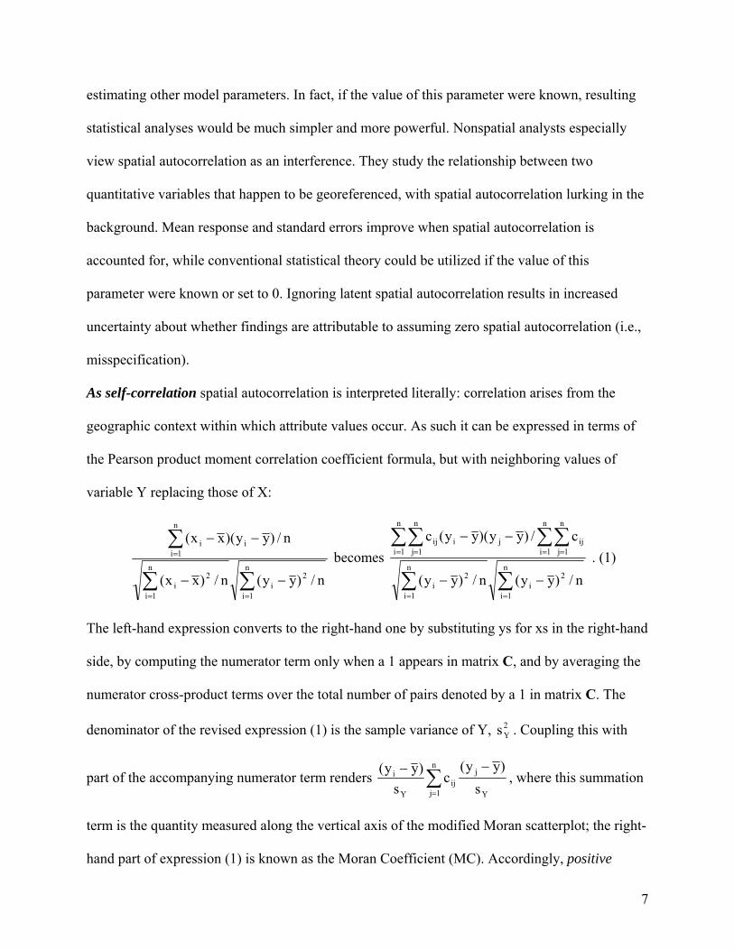
Figure 1. Adair County, Missouri, 1990 population density and census block areal units. Upper

left: binary geographic connectivity matrix C. Upper right: geographic distribution of population

density (with Kirkville as an inset). Lower left: Moran scatterplot for population density (cross)

and LN(population density + 164) (•). Lower right: semivariogram plot for LN(population

density + 164) (•) and its Bessel function predicted values (cross).