Embed Size (px)
Citation preview

Spatial and temporal variation in Kemp’s ridley abundance:
Patterns, mechanisms, and implications
Nathan F. PutmanLGL Ecological Research Associates Bryan, Texas USA
Outline
The migration triangle: linkages between life-stages
Mechanisms driving spatial variation in abundance
Mechanisms driving temporal variation in abundance Strandings as a possible recruitment index Can trends in strandings provide an indication of future nesting output?
Next steps needed
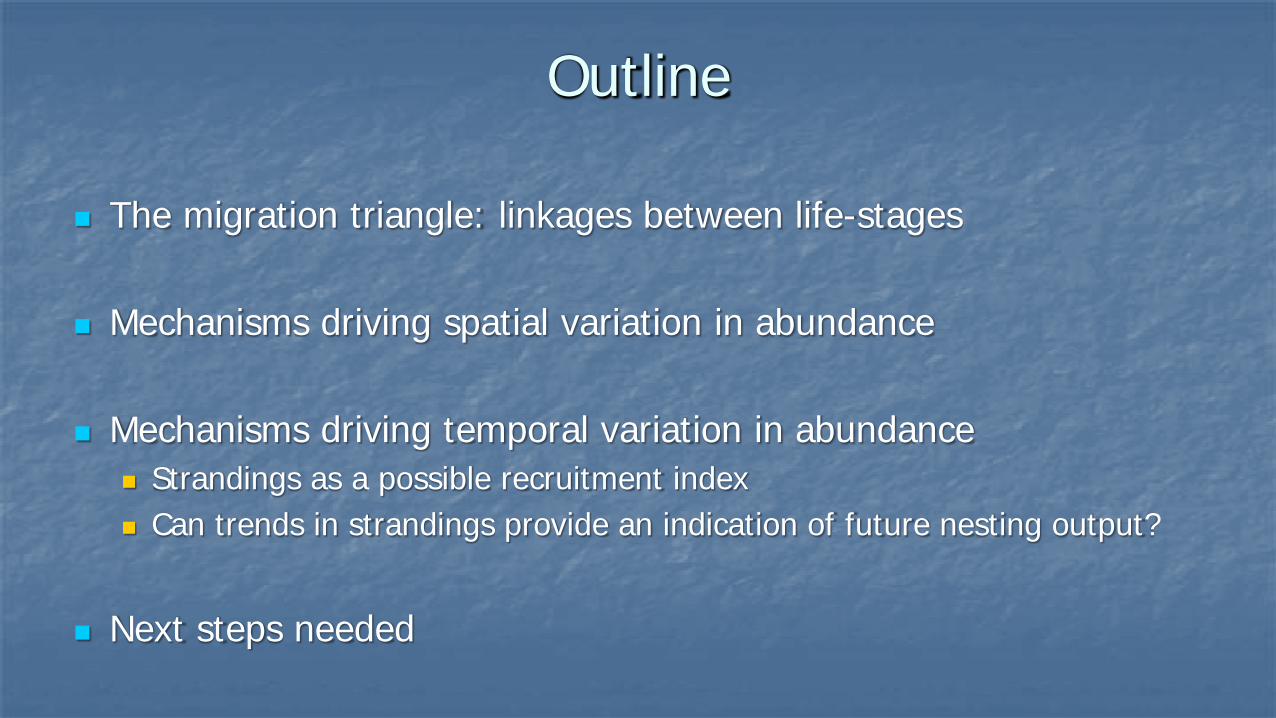
The migration triangle: linking life-stages
Reproductive Area
Nursery Grounds
Adult Foraging Grounds
Recruitment
Dispersal
Homing
Post-reproductivemovement
Adapted from Harden Jones 1968, Fish Migration
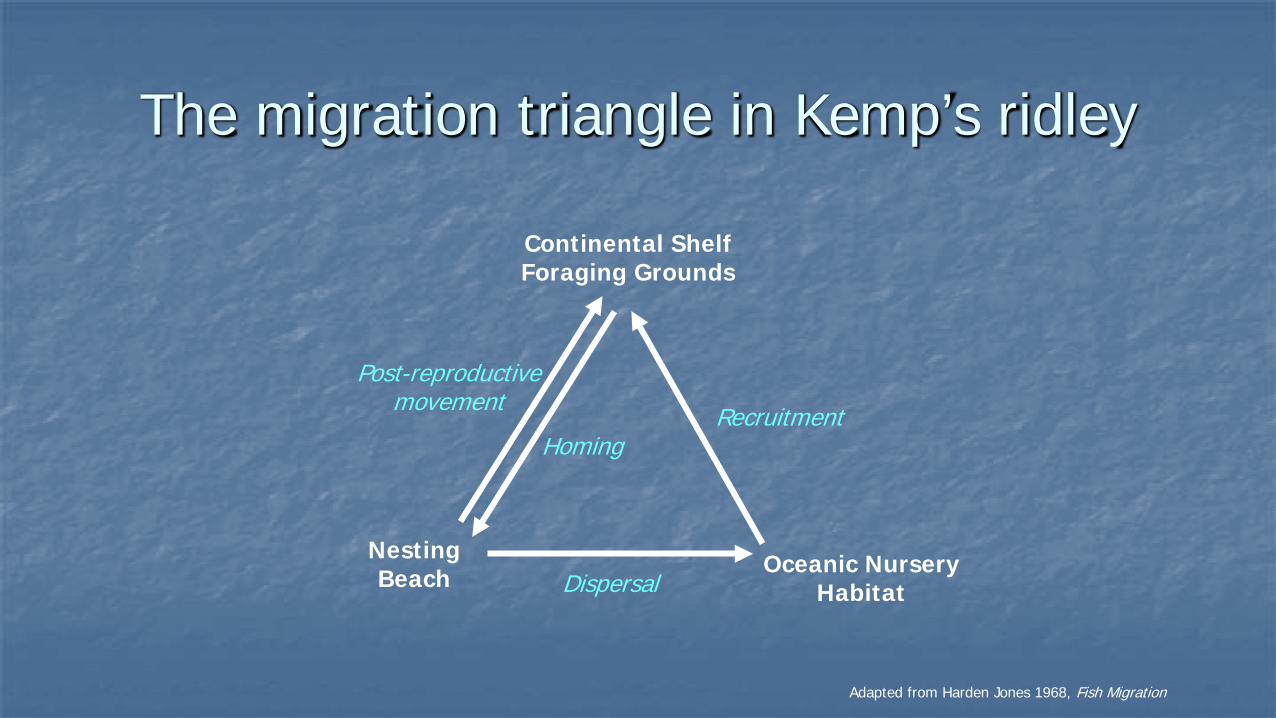
The migration triangle in Kemp’s ridley
Nesting Beach Oceanic Nursery
Habitat
Continental Shelf Foraging Grounds
Recruitment
Dispersal
Homing
Post-reproductivemovement
Adapted from Harden Jones 1968, Fish Migration

Putman et al. 2013, Biology Letters
The reproductive areas of Kemp’s ridley
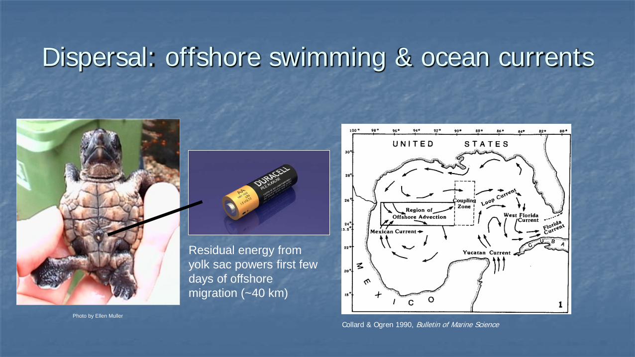
Collard & Ogren 1990, Bulletin of Marine Science
Dispersal: offshore swimming & ocean currents
Photo by Ellen Muller
Residual energy from yolk sac powers first few days of offshore migration (~40 km)

Dispersal & Recruitment: ocean currentsPredicted turtle density Predicted turtle age
Putman et al. 2013, Biology Letters
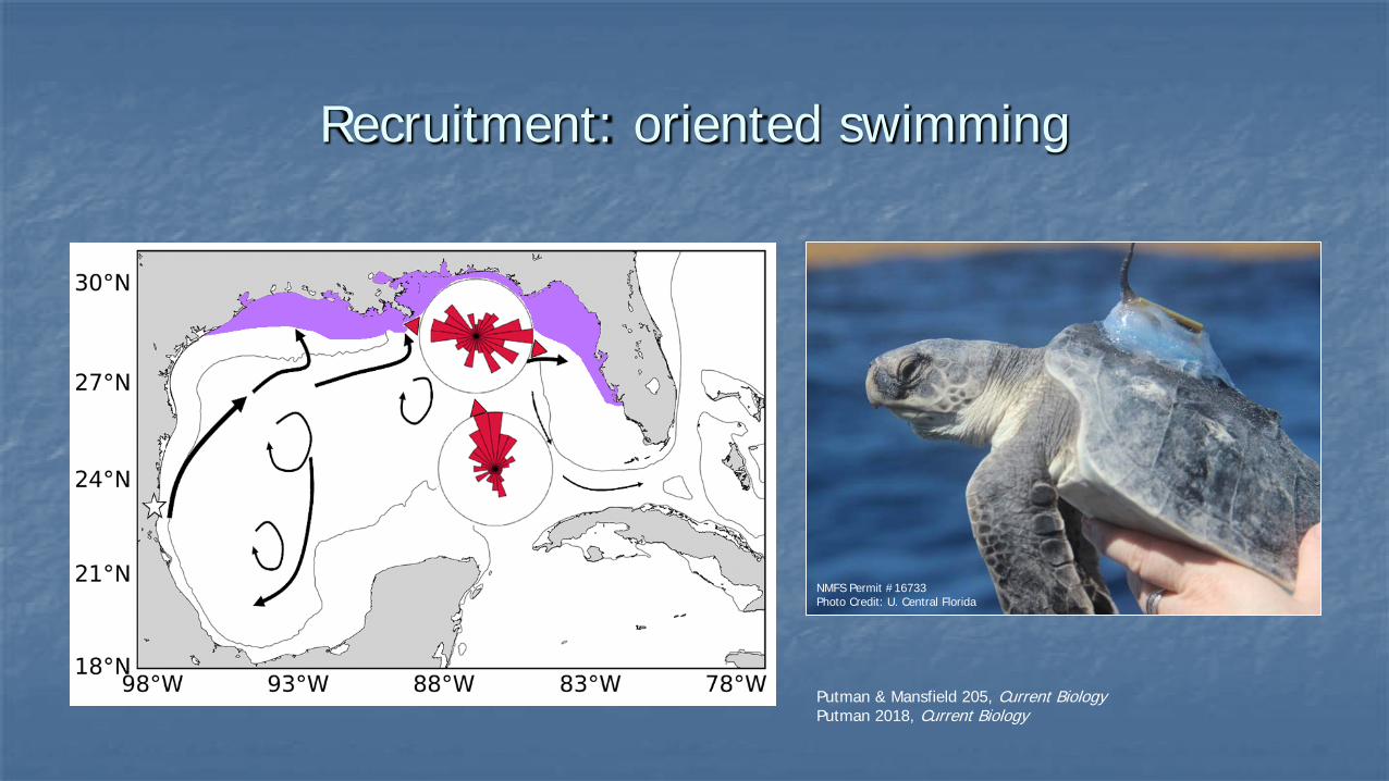
Recruitment: oriented swimming
NMFS Permit #16733Photo Credit: U. Central Florida
Putman & Mansfield 205, Current BiologyPutman 2018, Current Biology
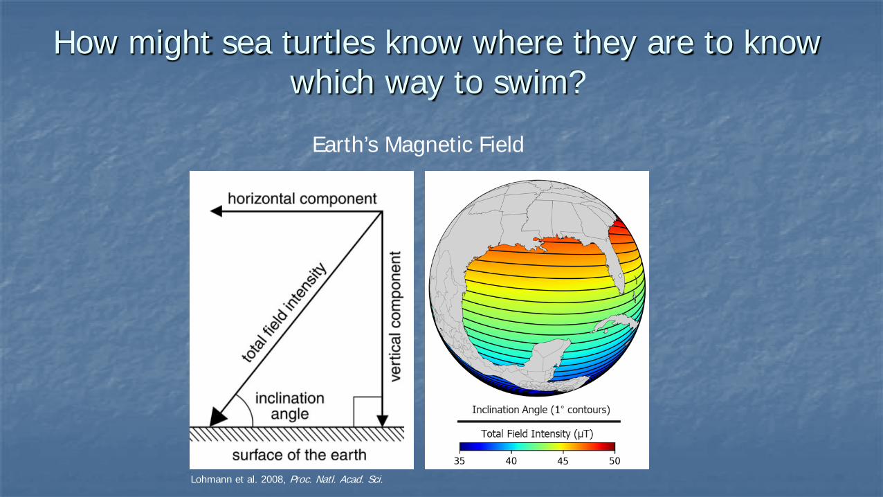
How might sea turtles know where they are to know which way to swim?
Lohmann et al. 2008, Proc. Natl. Acad. Sci.
Earth’s Magnetic Field
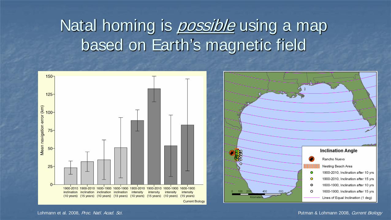
Natal homing is possible using a mapbased on Earth’s magnetic field
Putman & Lohmann 2008, Current BiologyLohmann et al. 2008, Proc. Natl. Acad. Sci.

Using the migration triangle in Kemp’s ridley to understand mechanisms of spatiotemporal variation in abundance
Ocean currents dominate movement; compass cues are most important
Swimming dominates movement; map cues are most important Swimming behavior and ocean
currents are important; map cues become increasingly important

Mean percentage of Kemp’s ridley nesting by state (2009-2011)
Putman 2018, Current Biology
Spatial variation in nest abundance is related to how well offshore conditions facilitate dispersal to nursery habitat
0
10
20
30
40
50
60
70
80
90
100
Texas Tamaulipas Veracruz
Nest
Abu
ndan
ce (%
)
Kemp’s ridley nesting regions

Is temporal variability in nest abundance related to recruitment dynamics?
0
5,000
10,000
15,000
20,000
25,000Kemp's ridley nest counts
Tamaulipas Texas Veracruz
Caillouet et al. 2018, Chelonian Conservation & BiologyShaver & Caillouet 2015, Herpetological Conservation & Biologyhttp://www.saveloraturtles.org/Jaime Pena

Using the migration triangle in Kemp’s ridley to understand mechanisms of spatiotemporal variation in abundance
Ocean currents dominate movement; compass cues are most important
Swimming dominates movement; map cues are most important Swimming behavior and ocean
currents are important; map cues become increasingly important
Does hatchling production predict future nesting?
Does recruitment predict future nesting?
~2 years
~10 years

The more hatchlings that were produced 12 years ago, the more nests now
Hatchlings Released: Spearman r = 0.870, p = 0.000000032
y = 6126.9ln(x) - 61359R² = 0.6774
0
5,000
10,000
15,000
20,000
25,000
30,000
0 200,000 400,000 600,000 800,000
Nes
ts
Hatchling Production

Can strandings data be used to estimate recruitment?
Research Team: Erin E. Seney, Melissa Cook, Allen M. Foley, Donna J. Shaver, Wendy G. Teas, Mandy C. Tumlin, and Katherine L. Mansfield
“New” Recruits: 21.3 – 42.5 cm CCL
0
50
100
150
200
250
Num
ber o
f Str
andi
ngs
Years
Tx_All La-Al_All Fl_AllAvens et al. 2017, PLoS One

Use strandings across Texas, Louisiana-Alabama, and Florida to predict nesting in Tamaulipas
Rationale: Anthropogenic drivers (e.g., bycatch) are certainly an issue, but we assume
variation in strandings is driven primarily by variation in abundance of turtles entering a region
Thus, we might expect the number of turtles that strand in a given year (at a size of 21.3 – 42 cm CCL) to correlate with the number of nests deposited 10 years later Oceanic dispersal stages ~ 2 years (< 21.3 cm CCL) Age at sexual maturity ~ 12 years (64.8 cm CL) i.e., 1985 strandings predict 1995 nesting… 2008 strandings predict 2018 nesting
Use non-parametric correlations (Spearman) to assess whether relationship exists between strandings and nesting
Use regression models to produce equations to “forecast” Kemp’s ridley nesting (2019 – 2024)
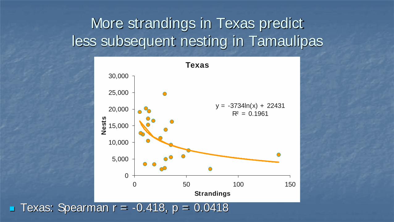
More strandings in Texas predict less subsequent nesting in Tamaulipas
Texas: Spearman r = -0.418, p = 0.0418
y = -3734ln(x) + 22431R² = 0.1961
0
5,000
10,000
15,000
20,000
25,000
30,000
0 50 100 150
Nes
ts
Strandings
Texas

No relationship between strandings in Louisiana-Alabama and nesting in Tamaulipas
Louisiana – Alabama: Spearman r = -0.141, p = 0.5113
y = -41.314x + 11929R² = 0.0216
0
5,000
10,000
15,000
20,000
25,000
30,000
0 20 40 60 80 100
Nes
ts
Strandings
Louisiana-Alabama

Florida: Spearman r = 0.823 , p = 0.000000782
More strandings in Florida predict more subsequent nesting in Tamaulipas
y = 221.53x + 3363.2R² = 0.5658
0
5,000
10,000
15,000
20,000
25,000
30,000
0 20 40 60 80 100
Nes
ts
Strandings
Florida

Forecasting Kemp’s ridley nesting
0
5000
10000
15000
20000
25000
30000
Nest
Cou
nts

Forecasting Kemp’s ridley nesting:Hatchling Production
0
5000
10000
15000
20000
25000
30000
Nest
Cou
nts
R2 = 0.67P = 0.0000008N=23

Forecasting Kemp’s ridley nesting:Recruitment to Florida (strandings)
0
5000
10000
15000
20000
25000
30000
Nest
Cou
nts
R2 = 0.56P = 0.000022N = 23

Forecasting Kemp’s ridley nesting:Production + Recruitment
0
5000
10000
15000
20000
25000
30000
Nest
Cou
nts
R2 = 0.78Production, P = 0.00016Recruitment, P = 0.0043N = 23

Possible Implications
Some regions are more suitable than others for maturing Kemp’s ridley in the northern Gulf. Fitness (survival, fecundity) is increased for juvenile turtles reaching
Florida and thus reproductive output increases. Kemp’s ridley reaching Texas arrive “too early” and are subject to higher
mortality than those recruiting at more eastern regions. Fairly robust statistical relationship between hatchling production
+ strandings and nesting suggests a 9 year forecast to set expectations for future population dynamics.
Next Steps Needed Build in corrections based on differences in probability of
strandings (e.g., observer coverage, wind/current conditions).
Consider correcting for anomalous occurrences (e.g., cold stuns, DWH oil spill)
Incorporate into a full population demographic model to account for the contributions of other age classes to nesting (e.g., previous strong/weak cohorts).

Next Steps NeededFocusing on the mechanisms that drive of spatial and temporal variation in abundance
is essential to understanding population dynamics of Kemp’s ridley

Acknowledgements
Erin E. SeneyKatherine L. MansfieldBenny J. GallawayCharles W. CaillouetMelissa CookAllen M. FoleyDonna J. Shaver Wendy G. Teas Mandy C. Tumlin

Sanity Check: Do juvenile Kemp’s ridley strandings correlate with
environmental data as expected?
Anthropogenic drivers (e.g., bycatch) are certainly an issue, but we assume variation in strandings is driven primarily by variation in abundance of turtles entering a region and not susceptibility to mortality
Simple Ocean Data Assimilation model (SODA)1980-2017 at 0.5° resolution
Monthly means for environmental variables that may influence probability of stranding (e.g., ocean currents, wind stress) and sea turtle occurrence/habitat (temperature, salinity, sea surface height, and mixed layer depth)

Months with more eastward wind predict fewer strandings; months with more northward wind predict greater strandings
Eastward wind stress vs. Texas strandings Northward wind stress vs. Texas strandings
Map coloration shows correlation coefficient for monthly winds at each Gulf of Mexico grid point and monthly strandings of juveniles in Texas (1980-2014, n = 420).