Dominik Wiedenhofer

Spatial and Socio-economic Drivers of Direct and

Indirect Household Energy Consumption in

Australia

S O C I A L E C O L O G Y W O R K I N G P A P E R 1 3 3

Dezember 2011 ISSN 1726-3816

Dominik Wiedenhofer, 2011: Spatial and Socio-economic Drivers of Direct and Indirect Household Energy

Consumption in Australia

Social Ecology Working Paper Number 133 Vienna, December 2011

ISSN 1726-3816

Institute of Social Ecology IFF - Faculty for Interdisciplinary Studies (Klagenfurt, Graz, Vienna) Alpen-Adria-Universitaet

Schottenfeldgasse 29 A-1070 Vienna

www.aau.at/socec workingpaper@aau.at

© 2011 by IFF – Social Ecology

Spatial and Socio-economic Drivers of Direct and Indirect Household Energy Consumption in

Australia*

Von

Dominik Wiedenhofer

* Masterarbeit verfasst am Institut für Soziale Ökologie (IFF-Wien), Studium der Sozial- und Humanökologie. Diese Arbeit wurde von Dr. Julia K. Steinberger betreut.

1

Abstract:

In this working paper the results of an investigation of the direct and indirect primary energy requirements of Australian households are presented. Urban, suburban and rural consumption patterns as well as inter- and intra-regional levels of inequality are analyzed and discussed. The drivers of energy consumption for different categories of energy requirements are identified and quantified. Conclusions about the relationship between energy requirements, household characteristics, urban form and urbanization processes in the Australian context are drawn.

Zusammenfassung:

Der Inhalt dieser Master Arbeit umfasst eine Untersuchung des direkten und indirekten Primärenergieverbrauchs australischer Haushalte. Urbane, suburbane und rurale Konsummuster wurden verglichen, sowie inter- und intra- regionale Ungleichheiten quantifiziert. Unter Anwendung eines multivariaten Regressionsansatzes konnten die unterschiedlichen räumlichen und sozio-ökonomischen Einflussfaktoren auf die Energieverbrauchsmuster identifiziert und quantifiziert werden. Basierend auf den Ergebnissen der Analysen lassen sich Schlussfolgerungen über den Zusammenhang von Energieverbrauch, Haushaltscharakteristika, urbaner Form und Urbanisierungsprozessen im Australischen Kontext ziehen. Acknowledgements

Many thanks go to Julia Karen Steinberger, who supervised me with great enthusiasm and patience and successfully guided me through the trials of advanced statistics, as well as giving some important nudges at several stages of the whole project. Manfred Lenzen also proved to be a great inspiration and support and I thank him for the generous amount of time he spent with me discussing various aspects of this work and Input-Output approaches in general. Christoph Plutzar played an important role in the beginning of this work and his GIS support is highly valued. Shonali Pachauri gave valuable comments on an early draft, which are highly appreciated. Furthermore I thank the University of Klagenfurt for supporting me with a travel grant, without which my stay at the University of Sydney would not have been possible. Any errors and gaps in the research presented in the remainder of this work are solely the responsibility of the author.

2

Table of Contents

1. Introduction ........................................................................................................................ 4

Research questions addressed in this study ......................................................................................... 5

2. What do we know about the Energy Requirements of Household Consumption? ............ 6

Defining System Boundaries and the Allocation of Indirect Requirements ....................................... 6

Studying Industrial Interdependence using Input-Output Analysis and Environmental Extensions .. 9

Overview of current Findings on Energy Requirements of Household Consumption ...................... 11

Discussion of the Drivers of Energy Requirements of Household Consumption ............................. 16

Critical Remarks and Research Gaps in the Literature ..................................................................... 18

3. Sustainability and Urban Form(s) .................................................................................... 19

The Importance of Cities ................................................................................................................... 19

Urban Form: Definitions, Ideals and Political Planning ................................................................... 19

4. Methodology and Data Sources ....................................................................................... 21

Data Sources ...................................................................................................................................... 24

Methodological and Data Limitations ............................................................................................... 25

5. Discussion of Results ....................................................................................................... 26

Regional Inequalities in Income and Energy Requirements ............................................................. 28

Cross-correlations of Socio-Economic and Spatial Variables ........................................................... 29

6. Discussion and Conclusions ............................................................................................ 33

7. References ........................................................................................................................ 35

8. Appendices ....................................................................................................................... 46

Appendix 1: Household Expenditure Survey Data and the Combination with Environmentally

Extended Input – Output derived Energy Intensities ........................................................................ 46

Appendix 2: GIS, digital boundaries and the districts of interest ...................................................... 47

Appendix 3: Weather Data, Heating Degree Days and GIS procedures ........................................... 50

Appendix 4: Calculation Method for the Area-based Gini coefficients of Energy Requirements .... 53

Appendix 5: The Household Expenditure Survey and Socio-Demographic Data – preparing for

statistical analysis .............................................................................................................................. 55

Appendix 6: Household Expenditure data by Australian and New Zealand Standard Industry

Classification (ANZSIC) ................................................................................................................... 55

Appendix 7: Composition of energy requirement categories for statistical analysis ........................ 64

3

List of Tables

Table 1: Correlation of socio-demographic attributes and energy requirements .................................. 23

Table 2: Spatial differences in per capita energy requirements (GJ/cap) and income .......................... 27

Table 3: AR-Gini coefficients for income and energy requirements .................................................... 29

Table 4: Regression models for total, indirect and direct requirements ................................................ 30

Table 5: Regression results for private and public transport, residential and food-related energy requirements .......................................................................................................................................... 31

Table 6: Overview of officical statistical districts and districts used in the study ................................ 47

Table 7: Districts were HDD values had to be approximated from weather stations in the vicinity .... 51

List of Figures

Figure 1: Global GHG emissions attributable to Investments, Government and Household Consumption (Hertwich, Peters, 2009) ................................................................................................... 9

Figure 2: Energy requirements of household consumption from 21 studies, (Hertwich, 2011), 1 kW = 30,7584 GJ ............................................................................................................................................ 11

Figure 3: Relationship between expenditure and energy requirements of Australian households in 1999 (Lenzen et al. 2008) ............................................................................................................................... 13

Figure 4: Energy intensities of consumption, by Income (Lenzen, 1998a: S. 511) .............................. 14

Figure 5: Relationship of expenditure and energy intensities of consumption, for 12 countries (Lenzen et al., 2006) ............................................................................................................................................ 15

Figure 6: Heating degree days for Australia's 85 regions (own calculations) ....................................... 25

Figure 7: Population density of Australia's south-east .......................................................................... 26

Figure 8: Regional profiling on socio-demographic variables .............................................................. 28

Figure 9: Spatial distribution of weather stations from which HDD values were derived .................... 51

Figure 10: 30 year average of annual HDD from the Australian Bureau of Meterology ...................... 52

Figure 11: Area based Lorenz curves I.................................................................................................. 54

Figure 12: Area based Lorenz curves II ............................................................................................... 54

List of Equations

(Equation 1) ............................................................................................................................................. 8

(Equation 2) ........................................................................................................................................... 21

(Equation 3) ........................................................................................................................................... 21

(Equation 4) ........................................................................................................................................... 21

(Equation 5) ........................................................................................................................................... 22

(Equation 6) ........................................................................................................................................... 22

(Equation 7) ........................................................................................................................................... 22

(Equation 8) ........................................................................................................................................... 50

(Equation 9) ........................................................................................................................................... 53

4

1. Introduction

The growing consumption of fossil fuels is one of the principal threats to global sustainability. Concurrently it has also been argued that the exponential increase in global primary energy consumption over the last century is directly linked to the functioning of the social and economic system (Sieferle, 1997; Fischer-Kowalski, Haberl, 2007; Fischer-Kowalski et al., 2011). The changes which have been induced by this energetic social metabolism at all scales and in all the regions of the world are unparalleled in human history (McNeill, 2000). Serious concerns have also been raised about the global production of conventional oil peaking now or in the next 10-30 years (Sorrell et al., 2010a, 2010b). Furthermore climate change can ultimately be expected to have dire consequences for ecological and social systems if the long term trend of increasing fossil fuel use does not change dramatically (Lynas, 2008). Some even argue that to some extent these outcomes cannot be avoided anymore, because of the inertia of political systems, individual consumer psychology and identity and strong time lags between cause and effect (Hamilton, 2010). Even more so it is highly desirable to achieve a thorough understanding of the structure, patterns and drivers of energy consumption, since they can indicate possibilities and barriers for change (Hertwich, 2005b). In this work, two different strands of research are being brought together to possibly shed some light on some of these issues. One important perspective on energy use in modern economies can already be found in Adam Smith’s writing (1776), stating that “Consumption is the sole end and purpose of all production” (cited in Lenzen et al. 2004). With this quote in mind, it becomes clear that all economic activities and especially energy use at all the stages of the economic process are ultimately aimed at final consumption. This fruitfully expands the notion of energy use from the conceptually straightforward usage of fuel or electricity, towards an understanding that all goods and services, actually every single consumption activity required energy to be used at some or several stage(s) of the economic process. This notion is highly important in times of green consumerism advocating some sort of ‘shopping our way out of environmental problems’, which does not seem to live up to its promise if dealt with in a perspective formally incorporating the indirect or embodied energy requirements of consumption (Alfredsson, 2004). Rather more this understanding of the complexity and interdependencies of modern production processes can contribute to a more substantial understanding of the challenges and possibilities for change, leading to a notion of a sustainable lifestyle transition (Lenzen et al., 2008). The second line of research on which this study draws has focused on structural and spatial determinants of energy use in two specific areas. Firstly, the influence of spatial configurations of settlements and cities on individual mobility behavior and the subsequent transportation energy use (Newman, Kenworthy, 1991; Kennedy et al., 2009). Secondly, issues around the quality and quantity of the housing stock influencing the residential energy use for heating and cooling. Both areas connect to the wider debate around the sustainability of ongoing urbanization around the globe, as well as possibilities for strategic interventions and economies of scale provided by cities (Jenks et al., 2000; Weisz, Steinberger, 2010). Furthermore this area provides a close link to the first strand of research mentioned above, insofar as it strives to improve our understanding of the physical barriers and eventual ‘promotors’ of a sustainable lifestyle transition. A third line of research, which would be highly relevant for the research questions laid out in the next section and the issues touched upon above encompasses more of a sociological,

5

psychological and institutional understanding of the ‘willingness to consume’ as a driving force of consumption (Röpke, 1999; Hamilton, 2010). The spatial configuration of residential and other land-uses can also be understood as a product of sociological and economic dynamics, for example as seen in such phenomena as residential self-selection (Knox, Pinch, 2006; Cao et al., 2009). Furthermore a cognitive geography approach could also shed additional light on the afore mentioned aspects by explicitly dealing with the way people perceive and make sense of their surroundings, for example when it comes to making choices on travel mode, extent and number of trips (Weichhart, 2008). Attempts to integrate some of these aspects empirically have been presented by (Wier et al., 2001) and (Abrahamse, Steg, 2009). Unfortunately explicitly dealing with these aspects of the research questions laid out in the next section cannot be incorporated into this study because they go well beyond the scope of a single master’s thesis. Further research would definitely be interesting in this context and could definitely add to the debate.

Research questions addressed in this study

For this study, the goal is to undertake a consistent, consumption-based and spatially explicit study of direct and indirect energy requirements of Australian households. After contrasting urban, suburban and rural consumption patterns we identify the drivers of energy requirements to gain additional insights into the patterns of energy requirements of consumption and possibilities for intervention. The research focus of this thesis lies with the following five questions guiding the rest of this work.

- What are the levels and composition of direct and indirect energy requirements of Australian households?

- What influence do spatial considerations, such as urban form and urban-rural separation, have on the direct and indirect energy requirements of Australian households?

- What are the most important spatial and socio-economic factors influencing the energy requirements of Australian households?

- Can we distinguish typologies of direct and indirect energy requirements of households and urban form of Australian cities?

- What insights can be gained for guiding future urbanization and urban planning?

A theoretical discussion of existing findings from the literature in relation to the research focus will be followed by a brief treatment of the methodology applied. A longer discussion and analysis of results will then culminate in a tentative attempt to answer the fifth and arguable broadest research question.

6

2. What do we know about the Energy Requirements of Household

Consumption?

The goal of this section is to briefly discuss the basic assumptions of this perspective, give an overview of the most important findings in the current literature, critically evaluate these insights and identify relevant research gaps. From a consumption perspective, the primary energy supply of an economy, as well as the respective emissions caused and resources used, can be differentiated into the following two categories. Firstly, households, governments and businesses consume energy carriers in the form of heating and cooking fuels, electricity as well as petrol through driving a vehicle. These are usually defined as direct requirements. Secondly, the environmental pressure and resource depletion caused through the consumption of goods and services, which required energy and other resources for their production and delivery, are called indirect requirements

(Lenzen et al., 2008). Another commonly used term is embodied (Peters, Hertwich, 2008; Liu et al., 2010). These indirect requirements are generally understood to be of “infinite order”. “This means that they, in the case of the provision of a train journey for example, not only include environmental pressure caused by the very train journey, but also through assembling the train and running the stations, producing the steel for the train and the concrete for the station buildings, producing the materials for the steel and concrete factories, the machines to mine the iron ore, sand, etc, the steel to produce the mining equipment, and so on. This process of industrial interdependence proceeds infinitely in an upstream direction through the whole upstream life cycle of all products, like the branches of an infinite tree” (Lenzen et al., 2004). The sum of these direct and indirect requirements of resources, pollutants and energy is called total requirements.

The prinicipal method to investigate direct and indirect requirements and the underlying industrial interdependence is input-output analysis, as developed by Leontief (1936; 1970, among many other publications on the subject). For a general discussion of this approach, see section 0. For a more detailed description of the application in this study, see section 4. Another indicator on household consumption, which also has been developed early on, is the energy intensity of consumption. Energy intensity is defined as the fraction of energy requirements per currency unit spent, for example in GJ / Euro. The underlying interest is the fact, “that a consumer’s dollar [or Euro] can be spent with significantly different energy impact […]” (Herendeen, 1978). In effect, energy intensities of various expenditure categories are one of the most useful outcomes of input-output studies. This measure allows the investigation of the consequences of different consumption patterns as well as possibilities for reductions in total energy requirements through shifts in these patterns.

Defining System Boundaries and the Allocation of Indirect Requirements

One of the implicit starting points in all studies on energy / resource / emissions requirements of consumption is the way system boundaries are defined and whom the respective indirect requirements are being allocated to. Because of the large implications of differing system boundaries for the methodological effort as well as the scope of any investigation, this issue has received a lot of attention in the literature and policy arena (Lenzen, 1998a; Bastianoni et al., 2004; Munksgaard et al., 2005a). Three concepts have been put forward in this regard,

7

namely producer, consumer and recently also shared responsibility (Munksgaard, Pedersen, 2001; Lenzen et al., 2007a; Lenzen, 2007; Andrew, Forgie, 2008). In the producer perspective administrative and territorial borders (nations, states, regions) are defined as the relevant system boundaries. Therefore all resource and energy use as well as emissions resulting from activities within a given country are being allocated to that nation. This principle is currently the basis for national emissions accounting under the Kyoto Protocol and also underlies various initiatives targeted at the household or municipal level, like the Cities for Climate Protection program (CCP) or the International Council for Local Environmental Initiatives (ICLEI). Although a production based accounting scheme is conceptually and methodologically more straightforward, it suffers from the fact that it cannot take into account the upstream or indirect requirements of the activities happening in that given nation. This lead to concerns regarding ‘carbon leakage’ either in its weak form between annex B countries1, or even more importantly, as strong leakage from annex B countries to non-Annex2 countries (Hertwich, Peters, 2009). Especially strong carbon leakage can significantly undermine efforts to reduce the total GHG emissions of the world economy by allowing annex B countries to reach their GHG mitigation goals by effectively net importing embodied emissions, instead of reaching absolute reductions. Furthermore strong leakage can lead to economic inefficiencies, because emissions are potentially not abated where most cost effective, but by outsourcing production activities (Peters, Hertwich, 2006). (Weber, Matthews, 2008) estimated that in 2004 about 30% of the carbon emissions of US household consumption actually occurred outside the national borders. Australia ranks as a net exporter of CO2 emissions, with a 20% difference between the consumption and production accounting perspectives (Peters, Hertwich, 2008). These issues are even more pronounced at the sub-national level when comparisons are made between cities or regions (Weisz, Steinberger, 2010). Because cities are highly open economies and are inherently dependent on their hinterlands (Kennedy et al., 2007; Lenzen, Peters, 2010), a territorial or producer based accounting of indirect requirements cannot adequately capture the industrial interdependencies and different layers of production facilitating the consumption of goods and services in a city or region. Distinguishing between emissions and resource use occurring in a local area, with those resulting from the activities required to support the local population therefore again turns into the question of producer versus consumer responsibility (Munksgaard et al., 2005b). One interesting example for this issue is reported in (Lenzen et al., 2004): using the ICLEI-CCCP methodology3, the population of the city of Melbourne (including the CBD), has annual per capita emissions of 102 tons of CO2 equivalents. But the inhabitants of Frankston, a municipality in Melbourne, are only being estimated at 14 tons of CO2 equivalents. “This difference is however primarily due to the nature of the accounting of indirect emissions: people who happen to live in the CBD are largely not responsible for the large electricity use of that area which is required to service the businesses there.” (Lenzen et al., 2004). A territorial (production based) scheme of emissions accounting like the ICLEI-CCP results in the emissions being attributed to the resident population of that area, whether or not they actually benefit from these activities. If one is interested in a consistent investigation of the total requirements of consumption, it becomes therefore necessary to apply a strict consumption based accounting of energy and resource use as well as of the resulting emissions. This approach builds on Adam Smith’s

1 Annex B of the Kyoto Protocol contains a list of signatory nations which have agreed to legally binding GHG reduction goals 2 Non-Annex countries are developing and emerging economies of the Global South which did not agree to any binding GHG mitigation obligations under the Kyoto Protocol. 3 Australian Greenhouse Office and International Council for Local Environmental Initiatives 2000

8

(1776) notion, that “Consumption is the sole end and purpose of all production” (cited in Lenzen et al., 2004). This includes acknowledging that the majority of upstream production processes are ultimately intended and aimed at final consumption (Lenzen, 1998b). It then is plausible to fully assign the indirect requirements to the final consumers of the respective goods and services. Besides households, two other ‘final’ consumers are usually differentiated in macro-economics, namely government entities and investment activities of businesses. Different practices of accounting for the total requirements of these two other ‘final’ consumers can be found in the literature. On the one hand, it is sometimes argued that governments act for the people (by providing infrastructure, running public health systems, maintaining order and a legal system, ..) and that investments are necessary to maintain production (and consequently also consumption), so therefore households ultimately benefit from both (Lenzen, 1998a, 2001; Lenzen et al., 2004; Moll et al., 2005). In this view these requirements can be distributed equally among the population. This approach is seen as being better than not accounting for capital formation at all, but implicitly assuming a steady-state economy “is not entirely satisfying because capital expenditure varies annually, and a given year may not contain investment in new aluminum factories or automobile plants” (Hertwich, 2005b). On the other hand various authors do not include government consumption and investments in their analysis at all, or kept it as entirely separate categories (Herendeen, 1978; Vringer, Blok, 1995a; Weber, Matthews, 2008; Kerkhof et al., 2009; Hertwich, Peters, 2009; Shammin et al., 2010). Shammin et al. (2010) state that, “because taxes are a population’s collective input to government expenditures, and therefore it would not be justifiable to assign to individual consumers the energy burden resulting from the public expenditure of tax revenues”. This line of argument is based on the idea that household consumption is related to individual (consumer) choice and that the expenditures of governments and investments cannot be directly linked to the individual person, so therefore should not be assigned to his/her consumption pattern. As Herendeen (1978) puts it, “the dilemma therefore seems to be that this allocation appears different as viewed by the individual consumer looking out at the rest of society and the citizen looking in at his society”. Analytically this issue can be seen as the question what the ‘total cost of living’ for each citizen actually contains, which is ultimately an issue of definitions and research interest if all three terms are to be included (Equation 1, (expanded from Herendeen, 1978).

(Equation 1)

(Hertwich, Peters, 2009) results on the size of these three terms indicate, that this question is not just a matter of accounting principles (Figure 1). According to their estimate 72% of the global greenhouse gas emissions are related to household consumption, 10% to government consumption and 18% to investments.

9

Figure 1: Global GHG emissions attributable to Investments, Government and Household

Consumption (Hertwich, Peters, 2009)

Regarding a fair allocation of responsibility for energy use or greenhouse gas emissions, the concept of shared responsibility has recently been advanced. Neither a full producer nor consumer responsibility perspective seems perfectly appropriate when accounting for indirect requirements with the aim of enabling abatement activities under a post-Kyoto framework. To overcome this issue a consistent approach covering the complete life-cycle of all products and services, while avoiding problems of double-counting, has been formulated (Gallego, Lenzen, 2005; Lenzen, Murray, 2010). In this approach responsibilities for indirect requirements are shared between consumer and producer, either half / half or in relation to the value added, thereby explicitly linking responsibility with economic influence. For a longer discussion of the issues connected with shared responsibility and various stakeholder views, see (Lenzen et al., 2007b). In conclusion it is clear that assigning responsibility over the total requirements of goods, services and household consumption is not completely straightforward. Value judgments as well as different perspectives and scientific interests shape the definitions of system boundaries and the allocation procedures. For this work, following the research questions layed out in section 0 and the previous discussion, we are interested in a consistent, consumption-based perspective on the total energy requirements of Australian households. A discussion of the further implications and relations to the research focus of this study follows in the next sections.

Studying Industrial Interdependence using Input-Output Analysis and

Environmental Extensions

The study of industrial interdependence, using input-output methodology, goes back to the pioneering work of Wassily Leontief (1936; 1970, among many other publications), who developed and applied this method in a number of fields, thereby contributing richly to the

10

development of economics as a science and in its application to policy issues, projections, modeling exercises and other research areas (Duchin, 1992; Dorfman, 1995; Duchin, 1995; Augusztinovics, 1995; Rose, 1995). The notion of industrial interdependence is based on the fact that any given economic sector requires a multitude of different inputs, usually called intermediate demand, to produce its goods and services. “Input-output analysis describes and explains the level of output of each sector of a given national economy in terms of its relationships to the corresponding levels of activities in all the other sectors” (Leontief, Ford, 1970: S. 262). Because a large fraction of the economic activity of an economy is actually directed towards other sectors, it is highly important to incorporate these intermediate outputs into any analysis of the total requirements of production and consumption. “The implications of industrial interdependence, be it via sales (forward linkage) or purchases (backward linkage), are often crucial to the understanding of the effects of changes in economic circumstances both on particular industries and on the economy as a whole” (Dixon, 1996: S. 327). Direct requirements in this context refer to all the goods and services bought by a given sector from other sectors to produce its output. But every one of the supplying sectors also need intermediate inputs, which are again linked to the outputs of other sectors, and so forth. These upstream linkages towards all other sectors constitute the indirect requirements and are generally understood to be of infinite order (Lenzen et al., 2004). When the economic process is viewed in this fashion, it becomes clear that all sectors are directly or indirectly interconnected and that changes in any sector or of final demand, to some extent affect all other sectors as well. With this approach it is possible to model the total economic effects of for example changes in household final demand (Alfredsson, 2004; Abrahamse, Steg, 2009), government outlay options (Lenzen, Dey, 2002), different production technologies and price effects (Duchin, Lange, 1995), international trade patterns (Hertwich, Peters, 2009), distribute environmental responsibility for production and consumption activities equitably among different actors (see discussion on shared responsibility in section 0), assess individual and systems level rebound effects (Alfredsson, 2004; Hertwich, 2005a), investigate aspects of waste generation and treatment (Dietzenbacher, 2005) and many others. For a collection of recent applications and advances in the application of Input-Output economics in the field of Industrial Ecology, see (Suh, 2010). Any Input-Output analysis is based on a matrix representation of the inter-industry transactions in a given year. These are usually compiled by Statistical Offices and contain a complete table off all the monetary flows between sectors and to final demand (see for example ABS 2009 for Australian data). “These tables quantify for a given year the flows of goods and services, and of capital and labor, from one sector the other sectors and to final users” (Duchin, 1992: S. 852). To incorporate biophysical relevant information into these monetary models, so called environmental extensions are frequently used. These extensions, often compiled by statistical offices (for example NAMEA in the European Union), contain information on sectoral energy use, emissions, waste production and other relevant parameters. These can be coupled with monetary IO tables, thereby constituting for example direct and indirect energy intensities of sectoral production (or final consumption) (Lenzen, 2001). These can then be used to study the environmental impacts of different sectors and changes in the production outputs. The field of Environmentally Extended Input-Output analysis (EE-IO) has seen a rapid increase of publications since the mid 1990s (Hoekstra, 2010). See (Lenzen, 2001) for a thorough mathematical treatment of the formulation of a current EE-IO model, incorporating primary energy requirements as well as GHG emissions from other sources. For an overview of recent trends and developments in the field of EE-IO, see (Hoekstra, 2010).

11

Overview of current Findings on Energy Requirements of Household

Consumption

Since the pioneering studies of the 1970’s conducted by Herendeen and colleagues, a substantial body of research has been accumulated on household energy requirement patterns, the energy intensity of different consumption categories and the respective total costs of living. These early publications already present some important findings, for example that the indirect fraction ranged from one third to half of the total energy requirements of household consumption in the US and Norway of the 1970s (Herendeen, 1978; Herendeen et al., 1981). More recent studies have shown that in industrialized countries the fraction of indirect requirements has increased and is now on a par with, or even greater than direct energy requirements (Figure 2) and (Lenzen, 1998a; Moll et al., 2005; Hertwich, 2005b; Jackson, Papathanasopoulou, 2008). For those developing countries which have been investigated yet, indirect requirements are found to be on par or slightly below direct energy use (Pachauri, Spreng, 2002; Pachauri, 2004; Cohen et al., 2005; Park, Heo, 2007). Figure 2: Energy requirements of household consumption from 21 studies, (Hertwich, 2011), 1

kW = 30,7584 GJ

Furthermore large variations in total per capita primary energy requirements between countries can be observed, ranging from 283 GJ for the USA (in 2002), to 138 GJ for the UK (in 1996), to 12 GJ in India (in 1993-95) (Figure 2, own calculations). Moll et al. (2005) find per capita requirements of 112 GJ for the Netherlands, 135 GJ for the UK, 123 GJ for Sweden and 130 GJ for Norway. From Figure 2 it becomes furthermore clear that household energy (residential), vehicle fuel and other mobility (transportation requirements) and food compromise the largest fractions of the total energy requirements of households. Regarding energy intensity, most studies find that transportation, housing and food are the most energy intense consumption categories (Lenzen, 1998a; Moll et al., 2005). (Tukker, Jansen, 2006) furthermore corroborated this finding in their meta-study and conclude that these three

12

categories are responsible for 70% of the environmental impacts of final consumption in the EU, while only representing 55% of the expenditure (measured as energy use, CO2 equivalents, resource use, land use, acidification and smog formation). The dominant fraction in transportation energy requirements is direct energy use in the form of fuels for cars, motorbikes, etc. These end-user fuels like petrol also have a small indirect component to them, mainly from processing and distribution activities. The energy requirements of public transportation (fuel for buses, electricity for subways, etc) also fall under this category. Thirdly the smallest fraction, which is not always being included, is the embodied or indirect energy requirements of cars, buses and the relevant services like mechanics. Hertwich (2011) found in his meta-review across a large number of studies that mobility, including vehicle purchase and public transportation accounts for 23 +/- 8 % of the total requirements of average households. Housing or residential primary energy requirements include direct energy use for heating and cooling purposes, as well as electricity use in the home. All of these also have indirect components from their relevant production process, delivery and so forth. Hertwich (2011) also includes the indirect energy component from the construction, maintenance and furnishing of homes in his analysis and finds that all of these amount to 44 +/-9% of the total energy requirements of households. Food has both nutritional and indirect energy components: a 3000 kcal/day diet corresponds to 4.5 GJ per year in ‘nutritional’ energy per person. For this study the interest lies with the commercial primary energy required to produce, distribute and store food products. It can range from 2.5 to 4 GJ per capita per year for Indian urban households and 6 to 30 GJ for Brazilian urban households (where the ranges correspond to low and high income brackets) to around 40 GJ per capita per year for European households (Vringer, Blok, 1995b; Pachauri, 2004; Cohen et al., 2005). On average, food accounts for 15 +/- 4% of the energy requirements of per capita consumption (Hertwich, 2011). Because most energy use for food production happens outside city boundaries, this is also an example of the importance of an end-use consumer perspective. Besides the above discussed aspects it is also quite interesting to investigate the composition of consumption patterns of different income groups. Such an analysis has already been conducted in the early stages of this field (Herendeen, 1978; Herendeen et al., 1981). Current studies reconfirm the observation that with rising income, direct energy requirements increase only weakly, while most of the additional expenditures are used for more goods and services (=indirect requirements) Figure 3 and (Reinders et al., 2003a; Moll et al., 2005). The same effect interestingly also holds for urban households in Brazil (Cohen et al., 2005).

13

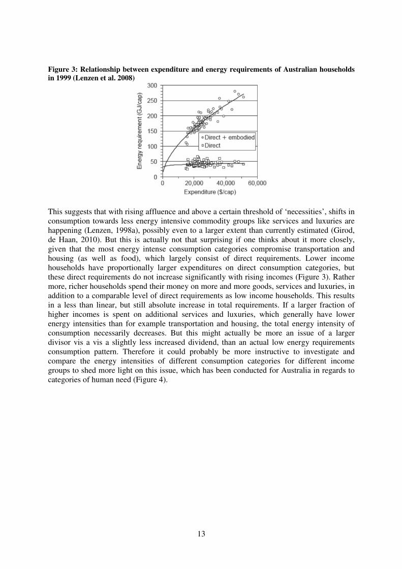
Figure 3: Relationship between expenditure and energy requirements of Australian households

in 1999 (Lenzen et al. 2008)

This suggests that with rising affluence and above a certain threshold of ‘necessities’, shifts in consumption towards less energy intensive commodity groups like services and luxuries are happening (Lenzen, 1998a), possibly even to a larger extent than currently estimated (Girod, de Haan, 2010). But this is actually not that surprising if one thinks about it more closely, given that the most energy intense consumption categories compromise transportation and housing (as well as food), which largely consist of direct requirements. Lower income households have proportionally larger expenditures on direct consumption categories, but these direct requirements do not increase significantly with rising incomes (Figure 3). Rather more, richer households spend their money on more and more goods, services and luxuries, in addition to a comparable level of direct requirements as low income households. This results in a less than linear, but still absolute increase in total requirements. If a larger fraction of higher incomes is spent on additional services and luxuries, which generally have lower energy intensities than for example transportation and housing, the total energy intensity of consumption necessarily decreases. But this might actually be more an issue of a larger divisor vis a vis a slightly less increased dividend, than an actual low energy requirements consumption pattern. Therefore it could probably be more instructive to investigate and compare the energy intensities of different consumption categories for different income groups to shed more light on this issue, which has been conducted for Australia in regards to categories of human need (Figure 4).

14

Figure 4: Energy intensities of consumption, by Income (Lenzen, 1998a: S. 511)

Lenzen (1998a: S. 511) concludes that this “[…] means that the commodities which are purchased by high income households but not by low income households are less energy intensive than the commodities purchased by both types of household. In other words, necessities are on average more energy intensive than luxuries, and the decrease of energy intensity with income is due to a saturation of necessities”. This indication of a curvature of total household requirements at higher income levels (Figure 3) and the decreases in energy intensity with higher incomes (Figure 4) lead to a revival of the Environmental Kuznets Curve (EKC) hypothesis. The EKC postulates that with rising incomes (or GPD or expenditure) at first environmental pressure increases, but at a certain turning point it starts to decrease again. This is presumably because “ […] (1) environmental quality is a luxury good, or results from (2) structural changes in the economy […], (3) equalizing income distribution, democracy and civil rights, or 4) technological progress (cleaner production and end-of-pipe technology, pollution prevention, material and energy efficiency)” (Lenzen et al., 2006: S. 184). In a multi-country study the relationship between energy intensity and different income levels has been investigated and it has become clear that with rising expenditure the energy intensity of consumption does decrease (Figure 5) (Lenzen et al., 2006).

15

Figure 5: Relationship of expenditure and energy intensities of consumption, for 12 countries

(Lenzen et al., 2006)

An attempt to calculate a hypothetical EKC turning point based on these decreases in total energy intensities and a slight saturation effect for total requirements, failed to produce any results anywhere close to observed levels of income (Lenzen et al., 2006). These results suggest that there is no EKC for the primary energy requirements of household consumption, now or in the near future. The total costs of living for urban versus rural households in relation to issues of urban sprawl have also been investigated early on. Herendeen et al. (1981: S. 72f) reported suburban and rural live in the USA and Norway to be 10% more energy intense than urban living in the 1960-70’s. This has been confirmed with similar results for Australia in the 1990s (Lenzen, 1998a; Lenzen et al., 2004) and the US for 2003 (Shammin et al., 2010). This means “[…] that the average person in a rural household spends their money on more energy intensive commodities than a person living in a city” (Lenzen, 1998a: S. 505). Based on various environmental pressure indicators Munksgaard et al. (2005a: S. 180) conclude that “[…] families living in rural houses perform the worst in terms of environmental friendliness, based on their relatively high consumption of [residential] energy and transportation.” Both consumption categories (as well as food) have been identified as most environmentally problematic (see above Tukker, Jansen, 2006). On the other hand, urban households show consistently higher levels of total energy and CO2 requirements than suburban or rural households, largely because of their higher incomes (Lenzen, 1998a; Wier et al., 2001; Lenzen et al., 2004). Concluding this suggests that, when differences in income are being controlled for, rural and sprawl living is comparatively more resource and energy intensive than urban lifestyles, mostly because of the larger share of transportation and residential energy requirements. This necessarily raises serious questions about the sustainability of urban sprawl and rural living in general and the respective possibilities for change. For urban dwellers the situation is slightly different, where structural aspects lead to lower direct energy use and lower energy intensities of consumption, but these inherently positive aspects are negated by significantly higher incomes and a generally more affluent lifestyle (Lenzen et al., 2008). But overall it becomes clear that serious progress in reducing total energy requirements

16

could be achieved by increasing the need for transportation and / or making it more energy efficient. The same goes for residential energy requirements.

Discussion of the Drivers of Energy Requirements of Household Consumption

Based on this overview of existing findings on energy requirements of household consumption, the respective drivers and influencing factors shall now be discussed. Across all studies, income / expenditure has been identified as the main determinant of total energy consumption (Herendeen, 1978; Reinders et al., 2003a; Moll et al., 2005; Lenzen et al., 2006). Expenditure is usually preferred to income as a predictor, because it corresponds more closely to what households actually consume (Wier et al., 2001). Expenditure includes social benefit transfers and various non-consumption expenses are already deducted, for example savings, taxes, donations and fines. Data on income levels on the other hand is much more readily available, for example from census data or international studies. This allows easier comparisons to other studies. Generally income / expenditure are much stronger causal variables regarding indirect than direct energy requirements (Figure 3) and (Reinders et al., 2003a; Lenzen et al., 2004). Another income/expenditure related variable is education. Usually education exhibits strong correlations with income (Lenzen et al., 2004). Using multivariate frameworks it has been shown that when expenditure is controlled for, weak negative influences on total requirements exist for Australia and the UK, while no significant impact has been found for Japan and Denmark (Lenzen et al., 2006; Baiocchi et al., 2010). For some this indicates possibilities for educated ‘green consumerism’ (Baiocchi et al., 2010), while Abrahamse and Steg (2009) point out, that while existing requirement patterns are explained quite well by socio-economic variables, energy savings and changes in consumption are much more associated with psychological factors. They conclude that “contextual variables such as income shape households’ opportunities for energy consumption, whereas reductions in energy use require conscious efforts to change behaviours/adopt energy-saving measures” (Abrahamse, Steg, 2009: S. 719). Unfortunately the variable education is not included in their statistical model, leaving the question unanswered what the exact link between these psychological factors and education is and if measures of levels of formal education could serve as a reliable proxy. Interestingly for developing countries like India and Brazil a positive link between education and total requirements has been reported (Cohen et al., 2005; Lenzen et al., 2006), where it has been hypothesized that especially urban educated individuals emulate a western consumerist lifestyle, which includes an ongoing accumulation of household stocks and consumer goods. Another important factor in understanding energy use is household composition and size – with more persons and especially more children resulting in reduced per capita consumption (Lenzen, 1998a; Wier et al., 2001; Lenzen et al., 2006). Because the energy intensities are the same for different household types, it can be deducted that the average composition of consumption stays the same (Lenzen, 1998a). Increased sharing of commodities therefore leads to lower per capita requirements, rather than a significantly different consumption pattern of different household types. Furthermore gender differences in energy requirement patterns of single men and women have been reported for four European countries. Single “women consistently used more energy than men […] [for] food, hygiene, household effects and health although differences are rather small.” (Räty, Carlsson-Kanyama, 2010: S. 648). Regarding transportation requirements and the category ‘restaurants, alcohol and tobacco’ men consumed considerably more energy. Furthermore significantly larger total requirements of men than women were found (Räty, Carlsson-Kanyama, 2010), although the authors unfortunately do not control for

17

income disparities statistically. Using data with several household types (not only singles), the independent effect of gender disappears (Abrahamse, Steg, 2009), but a significant correlation of gender and income is noted. This leaves the question unanswered if gender independently leads to significantly differing total requirements because of differences in expenditure patterns, or if this is a reflection of the general income disparities between men and women. Another influential demographic factor is age, which is found to have a positive effect on total requirements (Lenzen et al., 2006). Firstly, age is correlated with education and income, but even when these factors are controlled for, a small positive effect remains. Various explanations have been put forward, ranging from higher automobile mobility of independent retirees in Australia (NSW Department of Transport 2001, cited in Lenzen et al., 2006) to larger residential energy requirements because of relatively more time spent at home compared to working age persons, combined with possibly higher indoor temperatures to achieve comfort levels in seasonally cold countries. Regarding climatic influences, a close relationship with residential energy requirements for thermal comfort has been documented (Kennedy et al., 2009; Wang et al., 2010). Large variations besides climatic effects exist, which are related to the specific building envelope construction, heating system typology, thermal efficiency, controls, annual hours of use and highly important, occupant behavior (Balaras et al., 2005). In the context of direct and indirect requirements the influence of climate has not been quantified yet. Reinders et al. (2003b) do correct for it, but then only apply a univariate analysis with expenditure as explanatory variable, therefore not statistically capturing the independent effect of climate. Another study even failed to find a significant effect associated with climate variables, but as the author notes, this could also be the case of a spatially restricted sample (Sydney only) which could lead to climatic effects misleadingly being attributed to other variables (Rickwood, 2009) or simply not showing up because of a lack of variation in the data. For the variable population density a weak negative influence on total household energy requirements has been found for several countries, even when expenditure is being controlled for (Lenzen et al., 2006). Many urban energy studies have noted the importance of high population density as a factor in reducing private transport energy requirements (Newman, Kenworthy, 1991; Brown et al., o. J.; Kennedy et al., 2009). Dense urban form is also a prerequisite for an efficient and attractive public transportation system, as well as greater possibilities for walking and cycling because of shorter distances (Grazi et al., 2008). In response it has been argued that this influence might actually be more of an issue of attitude induced residential self-selection4, rather than an actual influence of the built environment on individual decision making. In a meta-review across 38 studies, Cao et al. (2009) found strong evidence suggesting that the built environment does indeed influence travel behavior, even when self-selection processes are controlled for. Furthermore higher density urban form also means more attached dwellings and especially flats and less separate houses. This potentially leads to lower residential energy requirements because of shared walls, smaller living space per capita and potentially also more efficient heating technology such as district heating or natural gas – although these possibilities are not always fully realized (Rickwood, 2009). Furthermore, it has also been suggested that above a certain threshold, densification might lead to disproportionately large increases in embodied energy for infrastructure and dwelling constructions (Rickwood et al., 2008). But this issue is still topic of ongoing research. For a further discussion on issues of urban form see section 3.

4 Self-selection describes the phenomena that people tend to choose their residential location based on their

preferred travel modes and needs. For a further discussion see the review by (Cao et al., 2009).

18

Another variable which is related to population density is ‘house type’, which is an index based on the local composition of flats, semi-detached dwellings and separate houses (from high to low index in the same order) used in various publications from Lenzen and colleagues. For Brazil, Denmark and India a positive relationship between total requirements and this house type index has been found, independent of income levels (Lenzen et al., 2006). To some extent this is an effect of this index serving as a proxy for the actual living space per capita - which means more space needing heating and light as well as possible efficiency gains for attached dwellings and flats (shared walls, etc) (Rickwood, 2009). Furthermore it has to be noted that this discussion of different drivers of energy requirements might implicitly suggest possibilities for change leading to savings in total energy requirements, for example due to lower private transportation requirements or intra-household sharing. But it is important to keep in mind that these changes do not automatically translate to proportionally lower total energy requirements, because of the well known rebound effect, also known as Jevon’s paradox (Hertwich, 2005a). This issue will be discussed further in the concluding section.

Critical Remarks and Research Gaps in the Literature

From this overview of the existing literature it becomes quite clear that some findings, like the relationship between direct and indirect energy requirements or the importance of income/expenditure, have been established quite well in the field. Others are still under debate, for example the exact impact of gender, nationally differing influences for education and also the exact role of population density. While income and expenditure elasticities of consumption have been a wide and fruitful topic of research, driving factors beside income/expenditure have only been investigated in some cases. Most studies only apply univariate methods, thereby possibly missing out on other influential variables, like those discussed in section 0. To investigate these impacts requires a multivariate regression methodology, coupled with enough data to make statistical statements viable. Furthermore rarely are more disaggregated consumption categories besides total, direct and indirect requirements being interrogated regarding their driving factors, which might be interesting to shed some light on different specific possibilities and barriers for change.

19

3. Sustainability and Urban Form(s)

The purpose of this section is to draw together points from the literature reviewed so far and put them into the context of the debates on the sustainability of cities and different settlement patterns in general.

The Importance of Cities

Cities are inherently dependent on their hinterlands (Bai, 2007a; Kennedy et al., 2007; Lenzen, Peters, 2010) and constitute an important nexus of production and consumption (Weisz, Steinberger, 2010). In connection with ongoing urbanization trends around the globe this has led to a surge of research activities in the relationship between cities and sustainability issues (Simon, 2007). Although cities are constrained by international economic processes, they can play a critical role within a multi-level governance approach necessary to effectively tackle issues of global climate change (Bulkeley, Betsill, 2005). Cities are furthermore places where resource and energy use meets local government capacities and therefore constitute one of the major avenues for the implementation and formulation for effective sustainability and climate policy (Bulkeley, Betsill, 2003). Policy instruments can generally be categorized as carrots (economic incentives), sticks (regulatory approaches) and sermons (information and educational instruments) (Bemelmans-Videc et al., 1998). For more detailed discussions on policy instruments on the urban level I have to refer the reader to the literature, for example in regard to transportation (Grazi, van den Bergh, 2008), urban energy policy options and its implications (Keirstead, Schulz, 2010), GHG mitigation in a suburban setting (Knuth, 2010) and for a more general treatment of the obstacles and beneficial pathways for the integration of different types of environmental concerns into urban management strategies (Bai, 2007b). A detailed discussion of energy requirements and the role of urban planning in combination with other policy instruments in the Australian context can be found in (Gray, Gleeson, 2007).

Urban Form: Definitions, Ideals and Political Planning

One of the widely discussed aspects of cities in the context of sustainability and climate policy relates to their physical structure, or urban form (various contributions in Jenks et al., 2000; Buxton, Scheurer, 2005; Gray, Gleeson, 2007; Grazi, van den Bergh, 2008). The term urban form and structure “[…] covers such aspects as density, geometric shape, use of land (residential, industrial) and infrastructure (road, rail, waterway), with implications for indicators such as density, fragmentation and accessibility” (Grazi et al., 2008: S. 97). Furthermore it “[…] refers to the arrangement of the larger functional units of a city, reflecting both the historical development of the city and its more recent planning history […]” (Rose, 1967). Urban form can be measured as population density (Newman, Kenworthy, 1991; Grazi et al., 2008; Kennedy et al., 2009). Generally more complex land-use indicators would be desirable, but are very complicated to construct, mostly only feasible for intra-city research and can rarely be used in international comparative studies (Rickwood, Glazebrook, 2009). They (2009) furthermore show that density can serve as useful proxy for more complex indicators. The impact of population density on different categories energy requirements has been discussed in section 0. The broader debate on the ideal urban form dates back to the early 19th century and most of the protagonists can be categorized as either ‘decentrist’ (dispersed and decentralized living) or ‘centrist’ (high density living) (Breheny, 1998). Breheney (1998) traces the origins of the debate in concerns about the effects of industrialization on cities in the 19th and early 20th

20

century and documents the renewed interest in large scale planning interventions with the birth of ‘sustainable development’ in the 1980s. Based on a review of the whole debate (up to the publication of book) he furthermore suggests a middle ground, incorporating the merits of all positions: “From the centrist case it can adopt continued, indeed tougher, containment, urban regeneration strategies, and a whole range of new intra-urban environmental initiatives. There will be environmental gains, but not at the expense of quality of life. From the decentrist case it can allow for the controlled direction of inevitable decentralization – to suburbs and towns able to support a full range of facilities and public transport, and to sites that cause the least environmental damage. It takes account of the grain of the market, without being subservient to it. It might allow for some development in the form of environmentally-conscious new settlements” (Breheny, 1998: S. 32). In connection it has been noted that the whole debate on sustainable cities is fraught with interests and values on what a city should be (Bulkeley, Betsill, 2003) and that strong ideological positions towards urban living strongly influences the various positions taken in the debate (Breheney 1998). Recent work has also argued for an understanding that there does not exist one ideal form, but many, depending on the local context, existing urban structure and political possibilities (Guy, Marvin, 2000). Forster (2006), based on a review of existing planning strategies throughout Australia concludes that the current ‘official’ vision of future urban structure in 20-30 years is one of “limited suburban expansion, a strong multi-nuclear structure with high density housing around centres and transport corridors, and infill and densification throughout the current inner and middle suburbs. Residents will live closer their work in largely self-contained suburban labour sheds, and will inhabit smaller, more energy-efficient and water–efficient houses. The percentage of trips using public transport, walking or cycling will have doubled. Regeneration programs will have broken up large concentrations of disadvantage, and […] low-income households will be able to find affordable dwellings […] within consolidation developments” (Forster, 2006: S. 179). These planning visions have been critiqued heavily for their overly narrow focus, based on the increasing geographical complexity of urban life in Australia (Forster, 2006). For further contributions on the implications and prospects for urban consolidation in the Australian context, see (Randolph, 2006; Buxton, Scheurer, 2005; Forster, 2006; Dodson, Sipe, 2008). The two consumption areas directly connected to urban form and structure are mobility and housing as well as their respective energy and resource requirements (Rickwood et al., 2008). Incidentally these have also been identified as the most energy intense and environmentally problematic consumption categories (see section 0 and (Moll et al., 2005; Tukker, Jansen, 2006). “The physical infrastructure of a particular neighborhood could be one key determinant of lifestyle-related emissions that could also act as a barrier to lifestyle change. Such potential infrastructure bottlenecks to emission reductions are still relatively little understood and are one important avenue of research […].” (Baiocchi et al., 2010: S. 67).

21

4. Methodology and Data Sources

In this study, input-output analysis coupled with spatially resolved household expenditure information is used to analyze the total primary energy consumption of households throughout Australia (see annex 0, 0). Environmentally extended input-output analysis can be used to model industrial interdependence and estimate the physical requirements of final demand in an economy (see also the discussion in section 0); for example, for energy, greenhouse gas emissions, pollutant emissions, nitrogen flows, water or ecological footprints (Leontief, Ford, 1970; Duchin, 1992; Dixon, 1996; Carter, Petri, 1989; Forssell, Polenske, 1998). This method was pioneered for energy in the 1970s (Herendeen, Sebald, 1975; Bullard, Herendeen, 1975; Herendeen, Tanaka, 1976) and has since been applied to many countries: Australia (Lenzen, 2001; Lenzen et al., 2008), Japan (Aoyagi et al., 1995), the Netherlands (Vringer, Blok, 1995b; Biesiot, Noorman, 1999; Weber, Perrels, 2000), Brazil (Cohen et al., 2005), Denmark (Munksgaard et al., 2000; Wier et al., 2001), the USA (Herendeen et al., 1981; Shammin et al., 2010) and India (Pachauri, Spreng, 2002). Three recent studies (Centre for Integrated Sustainability Analysis, Australian Conservation Foundation, 2007; Dey et al., 2007; Lenzen, Peters, 2010) achieved a complete household expenditure input-output map for energy, water and ecological footprints in Australia, which can be viewed on-line in the Australian Environmental Atlas, <http://www.acfonline.org.au>. Further explanations of the relevance of combining input-output methods and tables (ABS, 2009), energy statistics (ABS, 2003) and household expenditure data for the understanding of urban energy metabolisms can be found in Lenzen et al. (2008). Given this wealth of prior work, the standardization of the methodology and the scope of this study, the description of the methodology will be kept brief and the reader is referred to the existing literature, for example (Lenzen, 2001; Kok et al., 2006; Suh, 2010). Furthermore also annex 0 contains more detailed information. In essence, the national Australian input-output tables T (ABS 2009) and Australian energy statistics Q (ABARE, 2008) are combined in a generalized input-output analysis, national electricity data is replaced with region-specific values, and energy multipliers are calculate

(Lenzen, 2001), where holds gross economic output, and I is the identity matrix. (Equation 2) These multipliers are then applied to spatially disaggregated household expenditure data y from the Australian Household Expenditure Survey (HES, ABS, 2009), to yield indirect energy requirements. (Equation 3) Adding direct energy requirements Edir yield total energy requirements Etot.

(Equation 4)

The energy requirements for different categories of household expenditure, and for each spatial region of Australia, are then available for analysis. The HES also contains a range of socio-economic-demographic variables s, which we first submit to a correlation analysis in order to control for multicollinearity (Table 1, see also annex 0 for more information). For example, separate houses and the share of under 18-year-olds are closely correlated (0.8), which indicates that both variables express the same underlying issues and therefore possibly

22

lead to model misspecification when used simultaneously. These socio-economic, demographic and spatial variables are then used as explanatory variables in various multiple regression exercises of the form:

(Equation 5)

Given that

(Equation 6)

and in line with previous assessments (for example Wier et al., 2001), we interpret the ββββi coefficients as consumption-elasticities of energy requirements with respect to their socio-economic drivers si: as:

(Equation 7)

The interpretation of these elasticities is particularly straightforward: a 1% increase in the

explanatory variable si will result in a βi% change in energy consumption. Furthermore if ββββi

=1, the relationship is exactly proportional, if ββββi <1, the relationship is said to be inelastic, if ββββi

>1, the relationship is elastic (if ββββi <0, the same terms hold for - ββββi and the inverse of the socio-economic variable). The size of the respective student t – test additionally conveys information about the statistical significance of the interaction, with higher values indicating a stronger relationship. The goodness-of-fit statistic R

2 also contains valuable information insofar as it indicates what fraction of the variation found in the sample can be modeled by the regression.

23

Table 1: Correlation of socio-demographic attributes and energy requirements

n = 85 1 2 3 4 5 6 7 8 9 10 11

Income per capita 1 -0.56 0.50 0.52 -0.57 0.67 -0.18 0.47 -0.53 -0.27 -0.05 Separate dwellings 2 -0.56 -0.66 -0.76 0.80 -0.57 0.46 -0.40 0.83 0.41 0.17

Medium density 3 0.50 -0.66 0.65 -0.51 0.47 -0.24 0.63 -0.52 -0.35 -0.16

Apartments 4 0.52 -0.76 0.65 -0.65 0.45 -0.38 0.51 -0.64 -0.40 -0.25

Under 18-year-olds 5 -0.57 0.80 -0.51 -0.65 -0.61 0.60 -0.42 0.58 0.17 -0.02

18–64 years 6 0.67 -0.57 0.47 0.45 -0.61 -0.08 0.36 -0.46 -0.35 -0.15

Household size 7 -0.18 0.46 -0.24 -0.38 0.60 -0.08 -0.03 0.33 -0.13 -0.01

Population density 8 0.47 -0.40 0.63 0.51 -0.42 0.36 -0.03 -0.22 -0.20 0.02

To work by car 9 -0.53 0.83 -0.52 -0.64 0.58 -0.46 0.33 -0.22 0.62 0.22

Car ownership 10 -0.27 0.41 -0.35 -0.40 0.17 -0.35 -0.13 -0.20 0.62 0.35 Heating degree days 11 -0.05 0.17 -0.16 -0.24 -0.02 -0.15 -0.01 0.02 0.22 0.35

Total energy 12 0.80 -0.51 0.37 0.48 -0.57 0.47 -0.32 0.31 -0.53 -0.16 0.09

Indirect energy 13 0.82 -0.58 0.50 0.59 -0.58 0.53 -0.27 0.47 -0.59 -0.27 -0.05

Direct energy 14 0.05 0.21 -0.32 -0.31 -0.02 -0.06 -0.16 -0.42 0.18 0.29 0.42

Private transport 15 -0.17 0.29 -0.43 -0.41 0.13 -0.09 0.00 -0.46 0.28 0.31 0.18

Public transport 16 0.45 -0.43 0.62 0.52 -0.32 0.32 -0.11 0.72 -0.39 -0.38 0.01 Residential energy 17 0.29 -0.03 -0.03 -0.01 -0.21 0.07 -0.24 -0.13 -0.05 0.09 0.45 Food-related energy 18 0.72 -0.55 0.46 0.50 -0.63 0.54 -0.23 0.33 -0.51 -0.23 -0.06

Note: Values below 0.5 are printed in grey, values above 0.7 in bold for ease of reading

These socio-economic, demographic and spatial variables are then used as explanatory variables in various stepwise multiple regression analyses to identify the most relevant variables in the explanations of levels of energy consumption and to eliminate less significant influences which could potentially confuse the regression estimation. Therefore a cut-off point of t = 2.2 (~95% significance) has been chosen for model building. To avoid the omitted

variable bias, which occurs when relevant regressors are not included in the model, or issues of overfitting, which means that too many correlated variables are used for modelling, extensive testing has been conducted (Verbeek, 2008). Different variable combinations have been tried against relevant diagnostic statistics (students’ t tests, F tests between models, not using highly collinear variables simultaneously), theoretical expectations and the clustering of variables to find the most stable models and therefore relevant drivers.

Data Sources

The assembly of an Australian input-output table has been thoroughly described elsewhere, also the derivation of the respective energy intensities (Lenzen, 2001; Lenzen et al., 2004). The Australian Bureau of Statistics conducts regular household expenditure surveys (ABS 2000) whose data are released as average annual household expenditure per statistical district. For this work, a national dataset disaggregated into 85 districts is used where about half cover the major urban centres (Perth, Melbourne, Adelaide, Sydney and Brisbane) and the other half the rest of Australia. Heating degree days (HDD) were chosen as a proxy for climatic conditions They are frequently used for building energy demand management and approximate the heating needs of buildings in relation to a specified base temperature (Day, 2006; Kennedy et al., 2009; Hillman, Ramaswami, 2010). Data from 782 weather stations which are operated by the Australian Bureau of Meteorology were used to extrapolate average annual HDD for all 85 regions (see Figure 6 and annex 0 for more information). For comparison, Vienna has 1596, London 1053, New York 1238, Barcelona 368 and Tokyo 589 HDD. Generally the Australian climate is dominated by three climatic zones: tropical in the north-east, arid in the centre and western areas and temperate in the south-east (Peel et al., 2007). This roughly corresponds to the steadily increasing HDD values when moving from north to south(east).

25

Figure 6: Heating degree days for Australia's 85 regions (own calculations)

Methodological and Data Limitations

For a thorough treatment of the uncertainties and limitations of input-output models and survey data, see (Lenzen, 1998b; Lenzen et al., 2004; Kok et al., 2006; Girod, de Haan, 2010). Spatial datasets pose additional problems (Páez, Scott, 2005; Getis, 2007). First, the Modifiable Area Unit Problem relates to issues with the definition of boundaries for spatial districts and the subsequent process of aggregation (Openshaw, 1984; Atkinson, 2005). All studies based on spatially defined datasets (such as census data), are influenced by the underlying system of zoning and aggregation, which introduces additional uncertainties. The suggestions from the literature (using several different aggregation schemes, rastering of zonal data, individual level data) are not always possible and are still being researched. Second, geo-referenced variables often exhibit spatial autocorrelation, which means that not all observations in a spatial dataset can be assumed to be independent, violating the basic assumptions of any statistical analysis (Cliff, Ord, 1970; Páez, Scott, 2005; Getis, 2007). Moran’s I index is commonly estimated in order to address this issue, where the residuals of a regression analysis are tested to check if the regression model properly captures all spatial effects (Getis 2007). Moran’s I ranges from -1 to +1, where values around 0 indicate no spatial autocorrelation, while -1 / +1 means that there is perfect negative / positive autocorrelation.

26

5. Discussion of Results

As a first step, population density patterns have been used to divide Australia into three broad human settlement categories – urban, suburban and rural – as a basis for examining the differences and similarities in energy requirements between the residents of these regions. Secondly, the area-resource inequalities in energy requirements and income on a national level, and within the urban, suburban and rural classifications were quantified. Finally, multivariate regressions, using socio-economic and spatial variables to model nationwide energy requirements to identify the dominant drivers have been conducted. Differences and Similarities in Energy Requirements of Urban, Suburban and Rural Households At the time of census (2001) about 11.2 million people, or 64% of the population, lived in major urban centres (ABS, 2003). Melbourne, Sydney and Brisbane (Figure 2) are home to about 9 million people. The statistical district of Sydney has a population density of 3,291 persons / km², Melbourne 1,218 persons / km², Brisbane 3,483 persons / km², Perth 2,488 persons / km² and Adelaide 5,871 persons / km². Comparing these figures with population densities listed in Kennedy et al. (2009) indicates that Australian urban areas lie between the lower densities of North America (Denver 1,460, Los Angeles 905 and Toronto 772 persons / km²) and European cities (Barcelona 16,056 and London 4,664 persons / km²). Generally, in the Australian context, population density follows a steep gradient from high density areas in inner city districts to very low densities in suburban and rural areas (Figure 7). Figure 7: Population density of Australia's south-east

27

For the purpose of this study, urban areas are defined as districts with a population density of more than 1,000 persons/km², suburban areas with 1,000 to 100 persons/km² and rural areas with less than 100 persons/km². These ranges are based on two requirements: that districts with very low densities be clustered, and that districts connected with the CBDs of all five major cities be included in the ‘urban’ category. The remaining districts of these five major cities were defined as suburban. Based on these definitions, 24% of the Australian population lives in urban, 40% in suburban and 36% in rural areas (Table 2). To ensure that small modifications in the definition of the urban/suburban/rural boundaries do not lead to significant changes in the results, sensitivity analyses have been conducted. This is necessary to ensure that there are no districts close to the boundaries which strongly influence the results (for example with a population density of 999 persons / km² but a strongly different consumption pattern than all other suburban districts). The results shown below are robust under this sensitivity analysis, and therefore I am confident in the validity of our interpretations. Table 2: Spatial differences in per capita energy requirements (GJ/cap) and income

n = 85 Urban (n = 18) Suburban (n = 30) Rural (n = 37)

Annual income per capita

A$21,003 (4,798) A$17,729 (2,994) A$15,456 (2,766)

Annual income per household

A$51,572 (8,245) A$48,449 (9,696) A$39,978 (8,517)

Household size 2.5 (0.3) 2.74 (0.35) 2.58 (0.21)

Total energy 243 (34.7) 100% 218 (23.1) 100% 213 (20.5) 100%

Indirect energy 180 (30.9) 74% 152 (21.4) 70% 143 (18.2) 67%

Direct energy 63 (7.3) 26% 65 (7.8) 30% 69 (8.4) 33%

Private transport (direct)

25 (3.8) 10% 27 (3.9) 13% 30 (5.5) 14%

Public transport (direct)

2 (0.9) 1% 0.9 (0.6) 0.4% 0.5 (0.5) 0.2%

Residential energy (direct)

38 (4.9) 16% 37 (5.9) 17% 38 (6.2) 18%

Food-related (indirect)

21 (3) 9% 19 (2.1) 9% 18 (2) 8%

Population (%) 24% 40% 36%

Note: Figures in brackets are standard deviations

Annual per capita income is highest in urban areas, significantly less in the suburbs and lowest in rural areas: a 26 % decrease from urban to rural areas. For household income, the same trend is visible, namely 23% lower household incomes in rural areas, compared to the average urban households. The differences in total energy consumption are about half the income differences: a 12% decrease from urban to rural districts. Moreover, indirect energy is the dominant share in total consumption for all areas, representing over two-thirds of the total. Levels of direct consumption increase slightly from urban to rural, principally because of changes in transport energy requirements, with the more sparsely settled (and public transport poor) suburban and rural areas more dependent on private transportation. Residential energy

28

consumption is roughly the same for all three regional groupings, constituting a certain basic level of consumption which in relation to human needs could be interpreted as ‘necessities’ (Lenzen 1998a) – at least for the current Australian context, which is obviously not the worldwide norm. Food-related (indirect) energy is highest for the average urban inhabitant, with slightly lower levels for suburban and rural areas. Looking at the demographics of the urban/suburban/rural categories (Figure 8), shows that the shares of under 18-year-olds are significantly higher in suburban and rural areas than in urban areas. The strong population density gradient between urban and rural areas (Figure 7) is also evident in the shares of housing types, with significantly higher levels of flats and semi-detached houses in urban areas. The attributes relating to personal mobility reveal that the inhabitants of urban areas own significantly fewer cars and also use them less to get to work, compared to people living in suburban and rural areas. Figure 8: Regional profiling on socio-demographic variables

Regional Inequalities in Income and Energy Requirements

To further investigate urban/suburban/rural differences, area-resource (AR) Gini coefficients are calculated in order to quantify levels of inequality between districts (Druckman, Jackson, 2008b; Steinberger et al., 2010). The AR-Gini employs geographical distribution rather than income cohorts to measure inequalities, and can be used for energy or resource use as well as income (see annex 0 for more details).

29

Table 3: AR-Gini coefficients for income and energy requirements

National Urban Suburban Rural

Income per capita 0.32 0.20 0.31 0.33

Total energy 0.30 0.20 0.30 0.33

Indirect energy 0.32 0.18 0.32 0.34

Direct energy 0.28 0.23 0.25 0.31

Private transport 0.30 0.24 0.27 0.34

Public transport 0.46 0.24 0.43 0.51

Residential energy 0.27 0.22 0.25 0.29

Food-related energy 0.31 0.20 0.30 0.34 Note: 0 = perfect equality, 1 = total inequality

Nationwide income inequalities between districts reveal an AR-Gini coefficient of 0.32 (Table 3) The geographical distribution of the different categories of energy requirements is about as unequal as the income distribution, with the significant exception of public transport, with a much higher AR-Gini coefficient of 0.46. Because of the novelty of an area-resource Gini calculation, no international comparisons can be made at this point. When performing the same analysis on the subsets of urban, suburban and rural districts, the levels of intra-urban, intra-suburban and intra-rural inequalities are obtained. Typically, inequalities within more homogeneous areas are expected to be lower than nationwide. Indeed, ‘urban’ inequalities are much lower in all categories. For suburban areas they are only slightly below national levels. AR-Gini coefficients for rural areas are all somewhat higher than nationwide results. These elevated intra-rural inequalities are a sign that this regional category is more heterogeneous than either urban or suburban, which is not surprising: it encompasses rich coastal settled areas to the south-east as well as low income northern outback regions. (The attentive reader may have noticed that, upon first sight, this is in contradiction with the higher standard deviations for income found for urban areas (Table 2); this can be attributed to lower sample sizes for urban (n=18) than for suburban (n=30) and rural (n=37) areas, rather than inconsistencies in results.)

Cross-correlations of Socio-Economic and Spatial Variables

Additional insights into determinants of regional energy requirements and its spatial variability can be gained by isolating the effects of various explanatory factors utilizing a multivariate regression approach. For this purpose an analysis of the relationships between the explanatory variables and the energy consumption categories has been conducted (see Table 1). These interpretations could also be used to derive a typology of “typical” urban / suburban / rural average households. Generally the results confirm the socio-demographic consumption patterns of affluent inner urban dwellers vs car-dependent suburban and rural families. The first clustering of correlations can be identified around the variables semi-detached houses and flats which are predominantly found in inner urban areas, namely, income (+), population density (+), working age population (+), household size (-), to work by car and car ownership (-) as well as total, indirect, public transport and food-related energy requirements (+). A second clustering around the variable separate houses with income (-), population density (-), under 18-year-olds (+), household size (+), to work by car and car ownership (+) and total, indirect and food-related (-), but direct and private transport energy requirements (+) can also be found.

30

As expected, population density correlates positively with total, indirect and public transport energy consumption, and negatively with direct and private transport requirements. HDD also show the expected positive relationship with direct and residential energy requirements. Quantifying the Drivers of Energy Requirements through Multivariate Regression Analysis Income has a significant and strong influence on levels of total, direct and indirect energy requirements (Table 4). Comparing the β regression coefficients for income shows that this influence is not uniform, but much stronger for indirect than for direct requirements, while for total energy consumption the impact of income falls in between. Because the β regression coefficients can be interpreted like consumption-elasticities (see methods section), this means that changes in income levels can be expected to have the strongest influence on indirect energy requirements, and the least on direct energy consumption. Table 4: Regression models for total, indirect and direct requirements

n = 85 Total energy requirements

Indirect energy requirements

Direct energy requirements

β | t | β | t | β | t |

Income per capita 0.41 11.8 0.51 9.8 0.20 3.8

Household size -0.19 2.9 - - - -

Population density - - - - -0.02 6.4

To work by car - - -0.28 3.1 - - Heating degree days - - - - 0.03 5.4

R² 0.67 0.70 0.45

adj. R² 0.66 0.69 0.43

F stat 81.9 96.0 60.9

Moran’s I 0.02 -0.01 0.04 Note: Blank fields indicate that the variable was omitted in this model for reasons of colinearity or lack of

significance. The R2, F stat, t-statistic and Moran’s I are all described in the methodology section.

Household size has a significant negative influence on total energy requirements, possibly due to economies of scale caused by increased sharing of space and appliances among household members. This would lead to lower per capita expenditure on the goods and services affected by such household economies of scale. However, the shares of expenditures on various commodities do not change between large and smaller households, and the energy intensity of these consumption patterns is similarly unchanged (Lenzen 1998a). Indeed, it is surprising that the household size variable is only significant for total energy requirements, because other studies also identified it for direct and indirect energy requirements, although the strength of the effect tends to be much smaller than the one identified here (Wier et al., 2001; Lenzen et al., 2004; Cohen et al., 2005; Druckman, Jackson, 2008a). However, since I was using a different set of variables than the previous studies, it is possible that the household size influence seen in other studies appears in this work through these other variables. For instance the variable ‘travel to work by car’ is positively correlated with household size (Table 1) and its negative influence on indirect energy requirements could be seen by other studies with different variable sets as a household size effect. Indeed, our analysis reveals a negative influence of ‘travel to work by car’ on indirect energy requirements, even when controlling for differences in income levels between districts (Table 4). This means that independent of average incomes, higher shares of commuting by car are associated with lower average indirect energy consumption. This effect can be understood as a combination of car dependency, oil price vulnerability and high shares of mortgage financed

31

housing especially in suburban and rural districts having a strong adverse impact on household spending (Dodson, Sipe, 2007, 2008). As expected, heating degree days and population density have very significant, albeit weak, negative influences on direct energy requirements. Both are consistent with previous findings and are discussed below. A further disaggregation of direct (private and public transport as well as residential energy requirements) and indirect (food-related) consumption should yield additional insights (see Table 5). Table 5: Regression results for private and public transport, residential and food-related energy

requirements

n = 85 Private transport Public transport Residential Food-related

β | t | β | t | β | t | β | t |

Income per capita - - - - 0.35 5.0 0.31 6.3

Under 18-year-olds - - - - - - -0.15 3.9

Population density -0.02 4.3 0.2 9.0 -0.02 3.8 - -

Car ownership 0.38 2.4 -1.96 3.3 - - - -

Heating degree days - - - - 0.04 5.6 - -

R² 0.26 0.57 0.41 0.6

adj. R² 0.25 0.56 0.38 0.59

F stat 14.6 54.5 18.5 60.9

Moran’s I 0.15 -0.01 0.25 -0.01

The modelling suggests that income does not play a significant role for the determination of public or private transport energy requirements. Using the variables at our disposal, private transport energy requirements is best explained by population density and car ownership, although these only explain 25% of the variation in the data. The remaining spatial autocorrelation indicates that there are spatial processes at work which, with the variables at hand, cannot be captured properly (see Moran’s I, Table 5). The same variables, however with much higher coefficients and opposite signs, explain 55% of the variation in public transport energy requirements, with no spatial autocorrelation remaining in the model residuals. The connection between population density and levels of private transport energy requirements has been well documented (Newman, Kenworthy, 1991; Camagni et al., 2002; Grazi et al., 2008; Rickwood, Glazebrook, 2009). However, it is still not exactly clear what the causal links between population density and private transport are, besides the obvious shorter average distances travelled and greater public transport availability (Cameron et al., 2003). Car ownership rates can be understood as a combination of behavioural response to infrastructural issues (or urban form), social aspirations and income (Lenzen et al., 2008). Beyond private transport, the public transport result points to the same phenomenon: that mobility behaviour depends on availability and access to public transport infrastructure as well as broader issues related to urban form (such as mixed vs single use areas), spatial distribution of workplaces, facilities and shops, as well as individual preferences regarding automobile ownership and use (Camagni et al., 2002; Buxton, Scheurer, 2005; Grazi et al., 2008). Residential energy requirements can be modeled by income, population density and heating degree days, although these variables are still far from providing a satisfactory fit or removing the spatial autocorrelation from the data. The effects of income on this category are likely related to appliance ownership rates, floor sizes as well as individual heating behaviour. The negative influence of population density can be understood by less per capita floor space in

32

higher density residential areas where flats and semi-detached houses are dominant, which also tend to be more energy-efficient than separate houses. The effects of heating degree days are consistent with other findings (Kennedy et al. 2009). I find that the variable ‘under 18-year-olds’ exhibits a negative influence on food-related energy requirements, even when controlling for household income. Two explanations are possible here. First, lower dietary requirements of children compared to adults could lead to significantly less spending on food by the average family. Second, young families with children often live in car-dependent, mortgage-financed separate houses in suburban areas, which again leads to smaller per capita budgetary options for food (Dodson and Sipe 2007, 2008). Further research with household-level data and complementary information would be needed to explore either of these interpretations.

33

6. Discussion and Conclusions

To overcome some of the methodological and data limitations of this study, more detailed datasets, especially at an individual household level, are required. The limitations of averaged household data (Firebaugh, 2001) allows us to only draw general conclusions, in particular when it comes to potentials for intervention and changes at the individual level. More spatially disaggregated data would also yield more detailed insights into the relationship between urban form and different energy requirement categories and would almost definitely refine the results. This work has revealed significant differences in per capita energy requirement patterns for average urban, suburban and rural households throughout Australia. The results are consistent with earlier findings for Sydney (Lenzen et al. 2004): in the more urban and wealthier districts, indirect and total energy requirements are highest, while direct energy requirements is lowest compared to average suburban and rural households. Public transport energy requirements decrease steadily when moving from urban to rural districts, while private transport energy requirements increase. At equal incomes, districts with high levels of car dependency have lower levels of indirect energy requirements. Additionally, the lowest area-based inequalities for all energy requirement categories were found for urban districts, indicating more uniform consumption patterns than nationwide or in suburban and rural areas, which all have quite similar levels of inequality of energy requirements. The drivers of different energy requirement categories were explored using a combination of spatial and socioeconomic variables. Interestingly, income is far from playing a uniform role, since the income elasticities of energy consumption vary greatly: highest for indirect energy, and smallest for direct energy, with residential and food-related energy requirements between the two. Private and public transport energy requirements even seem to be independent of income and best modeled by car ownership and population density. There is a negative relationship between high rates of car ownership and lower average incomes (Table 1), while population density is positively correlated with higher incomes. This means that rising fuel costs are going to impact car-dependent and on average less affluent districts, such as most of the suburbs and rural Australia, much more than already wealthy urban areas, where there are also more possibilities and resources for adaptation, for instance, increased public transport use (Dodson and Sipe, 2008). In particular, suburban areas in their current form are locked into an energy intensive, automobile-dependent lifestyle built on uncontrolled low-density urban sprawl (Buxton, Scheurer, 2005; Gleeson, 2006; Frost, O’Hanlon, 2009; Spearritt, 2009). Policies which aim to decrease car use for the sake of the environment or public health have therefore to be carefully targeted so as not to disproportionately burden the lower income households through increasing prices. More importantly, issues of urban form have to be also taken into account, meaning that there need to be viable alternatives to automobile-based mobility such as serviceable public transportation systems, car sharing initiatives and alternative forms of transport to make changes possible. This is going to be a large challenge for most parts of Australia, especially outside the five major cities, where current very low density settlement patterns developed in combination with easy and cheap private automobile mobility. Furthermore, as our analysis shows, lowering private transportation energy requirements for environmental reasons may not be as effective as expected. In order to make these changes politically and socially viable, they would probably need to be cost saving in comparison to private car use, which in turn would lead to increases in indirect energy consumption (Table 4). This is an example of the household-level indirect rebound effect (Hertwich, 2005a). Although expenditure on indirect energy requirements is likely to be less energy intensive

34

than car use (Lenzen, 1998a), shifts in expenditure patterns from automobile use to other goods and services will lead to significantly lower reductions in total energy requirements than expected from the decrease in car use alone. The small but very significant influence of climatic conditions on residential energy requirements will have an increasing importance under future climate change, with increased pressure of the existing housing stock on local energy systems to be expected (Wang et al., 2010). Mitigation strategies need to take high efficiency standards for new buildings, improvements of the existing housing stock and future temperature levels as well as increased variability into account, so as not to overestimate potential gains (Wang et al., 2011). Following from all this, a new form of urbanism and human settlement patterns are necessary to enable households to actually decrease their total energy requirements. However, current developments in Australian urban and transport policy seem to keep focusing on large infrastructure projects as well as unchecked and hardly discussed (sub)urban sprawl (Dodson, 2009; Spearritt, 2009). Overall, it is also clear that the reductions required for serious climate change mitigation will be only possible with much more systemic and fundamental changes of production and consumption patterns than indicated here – a challenge faced by all developed and developing societies.

35

7. References

ABARE (2008): „Australian Energy Statistics: Australian Energy Update 2008“. Australian Government Retrieved am 23.05.2011 from http://www.abare.gov.au/interactive/energyUPDATE08/index.html.

Abrahamse, Wokje; Steg, Linda (2009): „How do socio-demographic and psychological factors relate to households’ direct and indirect energy use and savings?“. In: Journal

of Economic Psychology. 30 (5), pp. 711-720, doi: 10.1016/j.joep.2009.05.006.

ABS (2009): 1998-99 Household expenditure survey: detailed expenditure items. Canberra, Australia: Australian Bureau of Statistics.

ABS (2003): 2001 Census Household Sample File (CURF). Canberra, Australia: Australian Bureau of Statistics.

ABS (2000): Household Expenditure Survey: Summary of Results. Canberra, Australia: Australian Bureau of Statistics.

ABS (2001a): „Household income, living standards and financial stress“. In: Australian

Economic Indicators, June 2001. Canberra, Australia: Australian Bureau of Statistics.

ABS (2001b): Statistical Geography: Volume 1 Australian Standard Geographical

Classification (ASGC). Canberra, Australia: Australian Bureau of Statistics.

Alfredsson, E. C. (2004): „“Green” consumption--no solution for climate change“. In: Energy. 29 (4), pp. 513-524, doi: 10.1016/j.energy.2003.10.013.

Andrew, Robbie; Forgie, Vicky (2008): „A three-perspective view of greenhouse gas emission responsibilities in New Zealand“. In: Ecological Economics. 68 (1-2), pp. 194-204, doi: 10.1016/j.ecolecon.2008.02.016.

Aoyagi, M; Moriguchi, Y; Kondo, Y; et al. (1995): „Characteristics of household’s energy consumption“. In: Energy and Resources. (16), pp. 59-67.

Atkinson, Peter M. (2005): „Spatial Scale, Problems of“. In: Encyclopedia of Social

Measurement. New York: Elsevier pp. 639-648. — ISBN: 978-0-12-369398-3

Augusztinovics, Maria (1995): „What Input-Output is about“. In: Structural Change and

Economic Dynamics. 6 (3), pp. 271-277, doi: 10.1016/0954-349X(95)00016-G.

Bai, X. (2007a): „Industrial Ecology and the Global Impacts of Cities“. In: Journal of

Industrial Ecology. 11 (2), pp. 1-6.

Bai, Xuemei (2007b): „Integrating Global Environmental Concerns into Urban Management: The Scale and Readiness Arguments“. In: Journal of Industrial Ecology. 11 (2), pp. 15-29, doi: 10.1162/jie.2007.1202.

Baiocchi, Giovanni; Minx, Jan; Hubacek, Klaus (2010): „The Impact of Social Factors and Consumer Behavior on Carbon Dioxide Emissions in the United Kingdom“. In:

36

Journal of Industrial Ecology. 14 (1), pp. 50-72, doi: 10.1111/j.1530-9290.2009.00216.x.

Balaras, Constantinos A.; Droutsa, Kalliopi; Dascalaki, Elena; et al. (2005): „Heating energy consumption and resulting environmental impact of European apartment buildings“. In: Energy and Buildings. 37 (5), pp. 429-442, doi: 10.1016/j.enbuild.2004.08.003.

Bastianoni, Simone; Pulselli, Federico Maria; Tiezzi, Enzo (2004): „The problem of assigning responsibility for greenhouse gas emissions“. In: Ecological Economics. 49 (3), pp. 253-257, doi: 10.1016/j.ecolecon.2004.01.018.

Bemelmans-Videc, Marie-Louise.; Rist, Ray C.; Vedung, Evert (1998): Carrots, sticks, &

sermons: policy instruments & their evaluation. New Brunswick, N.J.; London: Transaction Publishers. — ISBN: 1560003383 9781560003380

Biesiot, Wouter; Noorman, Klaas Jan (1999): „Energy requirements of household consumption: a case study of The Netherlands“. In: Ecological Economics. 28 (3), pp. 367-383, doi: 10.1016/S0921-8009(98)00113-X.

Breheny, M (1998): „Centrists, Decentrists and Compromisers: Views on the Future of Urban Form“. In: Jenks, Mike; Burton, Elizabeth; Williams, Katie (eds.) The compact city: a

sustainable urban form? London, New York: E & FN Spon.

Brown, Marilyn, A.; Southworth, Frank; Sarzynski, Andrea (o. J.): Shrinking the carbon

footprint of metropolitation America. Washington, D.C.: Brookings Institution, 2008. (Metropolitatn Policy Program at Brookings).

Bulkeley, H.; Betsill, M. (2003): Cities and climate change: urban sustainability and global

environmental governance. New York: Routledge.

Bulkeley, Harriet; Betsill, Michele (2005): „Rethinking Sustainable Cities: Multilevel Governance and the “Urban” Politics of Climate Change“. In: Environmental Politics. 14 (1), pp. 42-63.

Bullard, Clark W.; Herendeen, Robert A. (1975): „The energy cost of goods and services“. In: Energy Policy. 3 (4), pp. 268-278, doi: 10.1016/0301-4215(75)90035-X.

Buxton, Michael; Scheurer, Jan (2005): The expanding urban frontier: urban form in

Melbourne’s growth areas. Melbourne, Australia: RMIT Publishing.

Camagni, Roberto; Gibelli, Maria Cristina; Rigamonti, Paolo (2002): „Urban mobility and urban form: the social and environmental costs of different patterns of urban expansion“. In: Ecological Economics. 40 (2), pp. 199-216, doi: 10.1016/S0921-8009(01)00254-3.

Cameron, I.; Kenworthy, J. R.; Lyons, T. J. (2003): „Understanding and predicting private motorised urban mobility“. In: Transportation Research Part D: Transport and

Environment. 8 (4), pp. 267-283, doi: 10.1016/S1361-9209(03)00003-8.

37

Cao, Xinyu; Mokhtarian, Patricia L.; Handy, Susan L. (2009): „Examining the Impacts of Residential Self-Selection on Travel Behaviour: A Focus on Empirical Findings“. In: Transport Reviews: A Transnational Transdisciplinary Journal. 29 (3), pp. 359-395.

Carter, Anne P.; Petri, Peter A. (1989): „Leontief’s contribution to economics“. In: Journal of

Policy Modeling. 11 (1), pp. 7-30, doi: 10.1016/0161-8938(89)90022-7.

Centre for Integrated Sustainability Analysis; Australian Conservation Foundation (2007): „ACF Consumption Atlas“. Retrieved am 23.05.2011 from http://www.acfonline.org.au/consumptionatlas/.

Cliff, Andrew D.; Ord, Keith (1970): „Spatial Autocorrelation: A Review of Existing and New Measures with Applications“. In: Economic Geography. 46 , pp. 269-292.

Cohen, Claude; Lenzen, Manfred; Schaeffer, Roberto (2005): „Energy requirements of households in Brazil“. In: Energy Policy. 33 (4), pp. 555-562, doi: 10.1016/j.enpol.2003.08.021.

Day, T (2006): Degree days: theory and application. London, UK: Chartered Institution of Building Services Engineers.

Dey, Christopher; Berger, Charles; Foran, Barney; et al. (2007): „Household environmental pressure from consumption: an Australian environmental atlas“. In: Birch, Gavin. (ed.) Water wind art and debate : how environmental concerns impact on disciplinary

research. Sydney: Sydney University Press. — ISBN: 9781920898656 1920898654

Dietzenbacher, Erik (2005): „Waste treatment in physical input-output analysis“. In: Ecological Economics. 55 (1), pp. 11-23, doi: 10.1016/j.ecolecon.2005.04.009.

Dixon, Robert (1996): „Inter-Industry Transactions and Input-Output Analysis“. In: Australian Economic Review. 29 (3), pp. 327-336, doi: 10.1111/j.1467-8462.1996.tb00939.x.

Dodson, Jago (2009): „The “Infrastructure Turn” in Australian Metropolitan Spatial Planning“. In: International Planning Studies. 14 (2), pp. 109-123.

Dodson, Jago; Sipe, Neil (2007): „Oil Vulnerability in the Australian City: Assessing Socioeconomic Risks from Higher Urban Fuel Prices“. In: Urban Studies. 44 (1), pp. 37 -62, doi: 10.1080/00420980601023810.

Dodson, Jago; Sipe, Neil (2008): „Shocking the Suburbs: Urban Location, Homeownership and Oil Vulnerability in the Australian City“. In: Housing Studies. 23 , pp. 377-401, doi: 10.1080/02673030802015619.

Dorfman, Robert (1995): „In appreciation of Wassily Leontief“. In: Structural Change and

Economic Dynamics. 6 (3), pp. 305-308, doi: 10.1016/0954-349X(95)00019-J.

Druckman, A.; Jackson, T. (2008a): „Household energy consumption in the UK: A highly geographically and socio-economically disaggregated model“. In: Energy Policy. 36 (8), pp. 3177-3192, doi: 10.1016/j.enpol.2008.03.021.

38

Druckman, A.; Jackson, T. (2008b): „Measuring resource inequalities: The concepts and methodology for an area-based Gini coefficient“. In: Ecological Economics. 65 (2), pp. 242-252, doi: doi: 10.1016/j.ecolecon.2007.12.013.

Druckman, A.; Jackson, T. (2008c): „Measuring resource inequalities: The concepts and methodology for an area-based Gini coefficient“. In: Ecological Economics. 65 (2), pp. 242-252, doi: 10.1016/j.ecolecon.2007.12.013.

Duchin, F (1992): „Industrial input-output analysis: implications for industrial ecology“. In: Proceedings of the National Academy of Sciences. 89 (3), pp. 851 -855.

Duchin, Faye (1995): „In honor of Wassily Leontief’s 90th birthday“. In: Structural Change

and Economic Dynamics. 6 (3), pp. 267-269, doi: 10.1016/0954-349X(95)00015-F.

Duchin, Faye; Lange, Glenn-Marie (1995): „The choice of technology and associated changes in prices in the U.S. economy“. In: Structural Change and Economic Dynamics. 6 (3), pp. 335-357, doi: 10.1016/0954-349X(95)00023-G.

Firebaugh, G. (2001): „Ecological Fallacy, Statistics of“. In: International Encyclopedia of

the Social & Behavioral Sciences. Oxford: Pergamon pp. 4023-4026. — ISBN: 978-0-08-043076-8

Fischer-Kowalski, Marina; Haberl, Helmut. (2007): „Socioecological transitions and global change trajectories of social metabolism and land use“. Retrieved am from http://site.ebrary.com/id/10328516.

Fischer-Kowalski, Marina; Mayer, Andreas; Schaffartzik, Anke (2011): „Zur sozialmetabolischen Transformation von Gesellschaft und Soziologie“. In: Handbuch

Umweltsoziologie. VS Verlag für Sozialwissenschaften pp. 97-120-120. — ISBN: 978-3-531-93097-8

Forssell, Osmo; Polenske, Karen R. (1998): „Introduction: Input-Output and the Environment“. In: Economic Systems Research. 10 (2), pp. 91-97.

Forster, Clive (2006): „The Challenge of Change: Australian Cities and Urban Planning in the New Millennium“. In: Geographical Research. 44 (2), pp. 173-182, doi: 10.1111/j.1745-5871.2006.00374.x.

Frost, L.; O’Hanlon, S. (2009): „Urban History and the future of australian cities“. In: Australian Economic History Review. 49 (1), pp. 1-18, doi: 10.1111/j.1467-8446.2008.00246.x.

Gallego, Blanca; Lenzen, Manfred (2005): „A consistent input–output formulation of shared producer and consumer responsibility“. In: Economic Systems Research. 17 (4), pp. 365-391.

Getis, Arthur (2007): „Reflections on spatial autocorrelation“. In: Regional Science and

Urban Economics. 37 (4), pp. 491-496, doi: 10.1016/j.regsciurbeco.2007.04.005.

39

Girod, Bastien; de Haan, Peter (2010): „GHG reduction potential of changes in consumption patterns and higher quality levels: Evidence from Swiss household consumption survey“. In: Energy Policy. 37 (12), pp. 5650-5661, doi: 10.1016/j.enpol.2009.08.026.

Gleeson, Brendan (2006): Australian heartlands making space for hope in the suburbs. [S.l.]: Allen & Unwin. — ISBN: 174115698X 9781741156980

Goodman, A; Oldfield, Z (2004): Permanent Differences? Income and Expenditure Inequality

in the 1990s and 2000s. London, UK: The Institute for Fiscal Studies.

Gray, Rowan; Gleeson, Brendan (2007): „Energy Demands of Urban Living: What Role for Planning?“. In: Adelaide, SA, Australia.

Grazi, F.; van den Bergh, J.C.J.M.; van Ommeren, J.N. (2008): „An empirical analysis of urban form, transport, and global warming“. In: Energy Journal. 29 (4), pp. 97-122.

Grazi, Fabio; van den Bergh, Jeroen C.J.M. (2008): „Spatial organization, transport, and climate change: Comparing instruments of spatial planning and policy“. In: Ecological

Economics. 67 (4), pp. 630-639, doi: 10.1016/j.ecolecon.2008.01.014.

Guy, S; Marvin, S (2000): „Models and Pathways: the diversity of sustainable urban futures“. In: Achieving sustainable urban form. London; New York: E & FN Spon. — ISBN: 0419244506 9780419244509

Hamilton, Clive. (2010): Requiem for a species: why we resist the truth about climate change. London; Washington, DC: Earthscan. — ISBN: 9781849710817 1849710813

Herendeen, Robert (1978): „Total energy cost of household consumption in Norway, 1973“. In: Energy. 3 (5), pp. 615-630, doi: 10.1016/0360-5442(78)90077-4.

Herendeen, Robert A.; Ford, Charlotte; Hannon, Bruce (1981): „Energy cost of living, 1972-1973“. In: Energy. 6 (12), pp. 1433-1450, doi: 10.1016/0360-5442(81)90069-4.

Herendeen, Robert; Sebald, A (1975): „Energy, employment and dollar impacts of certain consumer options“. In: Williams, R H (ed.) The energy conservation papers. Cambridge, Mass: Ballinger pp. 131-170.

Herendeen, Robert; Tanaka, Jerry (1976): „Energy cost of living“. In: Energy. 1 (2), pp. 165-178, doi: 10.1016/0360-5442(76)90015-3.

Hertwich, E. G. (2005a): „Consumption and the Rebound Effect: An Industrial Ecology Perspective“. In: Journal of Industrial Ecology. 9 (1-2), pp. 85-98, doi: 10.1162/1088198054084635.

Hertwich, Edgar G. (2005b): „Life Cycle Approaches to Sustainable Consumption: A Critical Review“. In: Environmental Science & Technology. 39 (13), pp. 4673-4684, doi: 10.1021/es0497375.

Hertwich, Edgar G. (2011): „The Life Cycle Environmental Impacts of Consumption“. In: Economic Systems Research. 23 (1), pp. 27-47.

40

Hertwich, Edgar G.; Peters, Glen P. (2009): „Carbon Footprint of Nations: A Global, Trade-Linked Analysis“. In: Environmental Science & Technology. 43 (16), pp. 6414-6420, doi: 10.1021/es803496a.

Hillman, Tim; Ramaswami, Anu (2010): „Greenhouse Gas Emission Footprints and Energy Use Benchmarks for Eight U.S. Cities“. In: Environmental Science & Technology. 44 (6), pp. 1902-1910, doi: 10.1021/es9024194.

Hoekstra, Rutger (2010): „(Towards) a complete database of peer-reviewed articles on environmentally extended input-output analysis“. In:

Jackson, Tim; Papathanasopoulou, Eleni (2008): „Luxury or “lock-in”? An exploration of unsustainable consumption in the UK: 1968 to 2000“. In: Ecological Economics. 68 (1-2), pp. 80-95, doi: 10.1016/j.ecolecon.2008.01.026.

Jenks, M.; Williams, Katie; Burton, Elizabeth (2000): Achieving sustainable urban form. London; New York: E & FN Spon. — ISBN: 0419244506 9780419244509

Keirstead, James; Schulz, Niels B. (2010): „London and beyond: Taking a closer look at urban energy policy“. In: Energy Policy. 38 (9), pp. 4870-4879, doi: 10.1016/j.enpol.2009.07.025.

Kennedy, Christopher; Cuddihy, John; Engel-Yan, Joshua (2007): „The Changing Metabolism of Cities“. In: Journal of Industrial Ecology. 11 (2), pp. 43-59.

Kennedy, Christopher; Steinberger, Julia; Gasson, Barrie; et al. (2009): „Greenhouse Gas Emissions from Global Cities“. In: Environmental Science & Technology. 43 (19), pp. 7297-7302, doi: 10.1021/es900213p.

Kerkhof, Annemarie C.; Benders, Ren M.J.; Moll, Henri C. (2009): „Determinants of variation in household CO2 emissions between and within countries“. In: Energy

Policy. 37 (4), pp. 1509-1517, doi: 10.1016/j.enpol.2008.12.013.

Knox, Paul Leslie; Pinch, Steven. (2006): Urban social geography : an introduction. New York: Pearson Education. — ISBN: 0131249444 9780131249448

Knuth, Sarah E. (2010): „Addressing place in climate change mitigation: Reducing emissions in a suburban landscape“. In: Applied Geography. 30 (4), pp. 518-531, doi: 10.1016/j.apgeog.2010.01.001.

Kok, Rixt; Benders, Ren M.J.; Moll, Henri C. (2006): „Measuring the environmental load of household consumption using some methods based on input-output energy analysis: A comparison of methods and a discussion of results“. In: Energy Policy. 34 (17), pp. 2744-2761, doi: 10.1016/j.enpol.2005.04.006.

La Cava, Gianni; Simon, John (2005): „Household Debt and Financial Constraints in Australia“. In: Australian Economic Review. 38 (1), pp. 40-60, doi: 10.1111/j.1467-8462.2005.00351.x.

Lenzen, Manfred (2001): „A Generalized Input–Output Multiplier Calculus for Australia“. In: Economic Systems Research. 13 (1), pp. 65-92.

41

Lenzen, Manfred (2007): „Aggregation (in-)variance of shared responsibility: A case study of Australia“. In: Ecological Economics. 64 (1), pp. 19-24, doi: 10.1016/j.ecolecon.2007.06.025.

Lenzen, Manfred (1998a): „Energy and greenhouse gas cost of living for Australia during 1993/94“. In: Energy. 23 (6), pp. 497-516, doi: 10.1016/S0360-5442(98)00020-6.

Lenzen, Manfred (1998b): „Primary energy and greenhouse gases embodied in Australian final consumption: an input-output analysis“. In: Energy Policy. 26 (6), pp. 495-506, doi: 10.1016/S0301-4215(98)00012-3.

Lenzen, Manfred; Dey, Christopher J. (2002): „Economic, energy and greenhouse emissions impacts of some consumer choice, technology and government outlay options“. In: Energy Economics. 24 (4), pp. 377-403, doi: 10.1016/S0140-9883(02)00007-5.

Lenzen, Manfred; Dey, Christopher; Foran, Barney (2004): „Energy requirements of Sydney households“. In: Ecological Economics. 49 (3), pp. 375-399, doi: 10.1016/j.ecolecon.2004.01.019.

Lenzen, Manfred; Murray, Joy (2010): „Conceptualising environmental responsibility“. In: Ecological Economics. 70 (2), pp. 261-270, doi: 10.1016/j.ecolecon.2010.04.005.

Lenzen, Manfred; Murray, Joy; Sack, Fabian; et al. (2007a): „Shared producer and consumer responsibility -- Theory and practice“. In: Ecological Economics. 61 (1), pp. 27-42, doi: 10.1016/j.ecolecon.2006.05.018.

Lenzen, Manfred; Murray, Joy; Sack, Fabian; et al. (2007b): „Shared producer and consumer responsibility -- Theory and practice“. In: Ecological Economics. 61 (1), pp. 27-42, doi: doi: DOI: 10.1016/j.ecolecon.2006.05.018.

Lenzen, Manfred; Peters, Greg M. (2010): „How City Dwellers Affect Their Resource Hinterland“. In: Journal of Industrial Ecology. 14 (1), pp. 73-90, doi: 10.1111/j.1530-9290.2009.00190.x.

Lenzen, Manfred; Wier, Mette; Cohen, Claude; et al. (2006): „A comparative multivariate analysis of household energy requirements in Australia, Brazil, Denmark, India and Japan“. In: Energy. 31 (2-3), pp. 181-207, doi: 10.1016/j.energy.2005.01.009.

Lenzen, Manfred; Wood, Richard; Foran, Barney (2008): „Direct versus Embodied Energy - The Need for Urban Lifestyle Transitions“. In: Urban Energy Transition. Amsterdam: Elsevier pp. 91-120. — ISBN: 978-0-08-045341-5

Leontief, Wassily W. (1936): „Quantitative Input and Output Relations in the Economic Systems of the United States“. In: The Review of Economics and Statistics. 18 (3), pp. 105-125.

Leontief, Wassily; Ford, D. (1970): „Environmental Repercussions and the Economic Structure: An Input-Output Approach“. In: The Review of Economics and Statistics. 52 (3), pp. 262-271.

42

Liu, Hongtao; Xi, Youmin; Guo, Ju’e; et al. (2010): „Energy embodied in the international trade of China: An energy input-output analysis“. In: Energy Policy. 38 (8), pp. 3957-3964, doi: 10.1016/j.enpol.2010.03.019.

Lynas, Mark (2008): Six degrees: our future on a hotter planet. Washington, D.C.: National Geographic. — ISBN: 9781426202131 142620213X 1426203853 9781426203855

McNeill, John. (2000): Something new under the sun: an environmental history of the world

in the twentieth-century. London: Allen Lane. — ISBN: 0713994622 9780713994629

Moll, H. C.; Noorman, K. J.; Kok, R.; et al. (2005): „Pursuing More Sustainable Consumption by Analyzing Household Metabolism in European Countries and Cities“. In: Journal

of Industrial Ecology. 9 (1-2), pp. 259-275.

Munksgaard, J.; Wier, M.; Lenzen, M.; et al. (2005a): „Using Input-Output Analysis to Measure the Environmental Pressure of Consumption at Different Spatial Levels“. In: Journal of Industrial Ecology. 9 (1-2), pp. 169-185.

Munksgaard, J.; Wier, M.; Lenzen, M.; et al. (2005b): „Using Input-Output Analysis to Measure the Environmental Pressure of Consumption at Different Spatial Levels“. In: Journal of Industrial Ecology. 9 (1-2), pp. 169-185.

Munksgaard, Jesper; Pedersen, Klaus Alsted (2001): „CO2 accounts for open economies: producer or consumer responsibility?“. In: Energy Policy. 29 (4), pp. 327-334, doi: 10.1016/S0301-4215(00)00120-8.

Munksgaard, Jesper; Pedersen, Klaus Alsted; Wien, Mette (2000): „Impact of household consumption on CO2 emissions“. In: Energy Economics. 22 (4), pp. 423-440, doi: 10.1016/S0140-9883(99)00033-X.

Newman, Peter W. G; Kenworthy, Jeffrey R (1991): „Transport and urban form in thirty-two of the world’s principal cities“. In: Transport Reviews: A Transnational

Transdisciplinary Journal. 11 (3), pp. 249 - 272.

Openshaw, S (1984): „Ecological fallacies and the analysis of areal census data“. In: Environment and Planning A. 16 (1), pp. 17-31.

Pachauri, Shonali (2004): „An analysis of cross-sectional variations in total household energy requirements in India using micro survey data“. In: Energy Policy. 32 (15), pp. 1723-1735, doi: 10.1016/S0301-4215(03)00162-9.

Pachauri, Shonali; Spreng, Daniel (2002): „Direct and indirect energy requirements of households in India“. In: Energy Policy. 30 (6), pp. 511-523, doi: 10.1016/S0301-4215(01)00119-7.

Páez, Antonio; Scott, Darren (2005): „Spatial statistics for urban analysis: A review of techniques with examples“. In: GeoJournal. 61 (1), pp. 53-67, doi: 10.1007/s10708-005-0877-5.

43

Park, Hi-Chun; Heo, Eunnyeong (2007): „The direct and indirect household energy requirements in the Republic of Korea from 1980 to 2000--An input-output analysis“. In: Energy Policy. 35 (5), pp. 2839-2851, doi: 10.1016/j.enpol.2006.10.002.

Peel, M.C.; Finlayson, B.L.; McMahon, T.A. (2007): „Updated world map of the Köppen-Geiger climate classification“. In:

Peters, Glen P.; Hertwich, Edgar G. (2008): „CO2 Embodied in International Trade with Implications for Global Climate Policy“. In: Environmental Science & Technology. 42 (5), pp. 1401-1407, doi: 10.1021/es072023k.

Peters, Glen P.; Hertwich, Edgar G. (2006): „Structural analysis of international trade: Environmental impacts of Norway“. In: Economic Systems Research. 18 (2), pp. 155-181.

Randolph, Bill (2006): „Delivering the Compact City in Australia: Current Trends and Future Implications“. In: Urban Policy and Research. 24 (4), pp. 473-490.

Räty, R.; Carlsson-Kanyama, A. (2010): „Energy consumption by gender in some European countries“. In: Energy Policy. 38 (1), pp. 646-649, doi: 10.1016/j.enpol.2009.08.010.

Reinders, A. H. M. E.; Vringer, K.; Blok, K. (2003a): „The direct and indirect energy requirement of households in the European Union“. In: Energy Policy. 31 (2), pp. 139-153, doi: 10.1016/S0301-4215(02)00019-8.

Reinders, A. H. M. E.; Vringer, K.; Blok, K. (2003b): „The direct and indirect energy requirement of households in the European Union“. In: Energy Policy. 31 (2), pp. 139-153, doi: doi: DOI: 10.1016/S0301-4215(02)00019-8.

Rickwood, Peter (2009): „Residential Operational Energy Use“. In: Urban Policy and

Research. Volume 27 (Number 2), pp. 137-155(19), doi: 10.1080/08111140902950495.

Rickwood, Peter; Glazebrook, Garry (2009): „Urban Structure and Commuting in Australian Cities“. In: Urban Policy and Research. 27 (2), pp. 171-188.

Rickwood, Peter; Glazebrook, Garry; Searle, Glen (2008): „Urban Structure and Energy—A Review“. In: Urban Policy and Research. 26 (1), pp. 57 - 81.

Röpke, Inge (1999): „The dynamics of willingness to consume“. In: Ecological Economics. 28 (3), pp. 399-420, doi: 10.1016/S0921-8009(98)00107-4.

Rose, Adam (1995): „Input-output economics and computable general equilibrium models“. In: Structural Change and Economic Dynamics. 6 (3), pp. 295-304, doi: 10.1016/0954-349X(95)00018-I.

Rose, Allen James. (1967): Patterns of cities. Melbourne, Australia: Nelson (Nelson’s Australasian paperbacks).

Shammin, Md. R.; Herendeen, Robert A.; Hanson, Michelle J.; et al. (2010): „A multivariate analysis of the energy intensity of sprawl versus compact living in the U.S. for 2003“.

44

In: Ecological Economics. 69 (12), pp. 2363-2373, doi: 10.1016/j.ecolecon.2010.07.003.

Sieferle, Rolf Peter (1997): Rückblick auf die Natur: eine Geschichte des Menschen und

seiner Umwelt. München: Luchterhand. — ISBN: 3630879934 9783630879932

Simon, David (2007): „Cities and global environmental change: exploring the links“. In: Geographical Journal. 173 (1), pp. 75-79, doi: 10.1111/j.1475-4959.2007.232_1.x.

Sorrell, Steve; Miller, Richard; Bentley, Roger; et al. (2010a): „Oil futures: A comparison of global supply forecasts“. In: Energy Policy. 38 (9), pp. 4990-5003, doi: 10.1016/j.enpol.2010.04.020.

Sorrell, Steve; Speirs, Jamie; Bentley, Roger; et al. (2010b): „Global oil depletion: A review of the evidence“. In: Energy Policy. 38 (9), pp. 5290-5295, doi: 10.1016/j.enpol.2010.04.046.

Spearritt, P. (2009): „The 200km city: brisbane, the gold coast and the sunshine coast“. In: Australian Economic History Review. 49 (1), pp. 87-106.

Steinberger, Julia K.; Krausmann, Fridolin; Eisenmenger, Nina (2010): „Global patterns of materials use: A socioeconomic and geophysical analysis“. In: Ecological Economics. 69 (5), pp. 1148-1158, doi: 10.1016/j.ecolecon.2009.12.009.

Suh, Sangwon. (2010): Handbook on input-output economics for industrial ecology. Dordrecht; London: Springer. — ISBN: 9781402061547 1402061544

Tukker, Arnold; Jansen, Bart (2006): „Environmental Impacts of Products: A Detailed Review of Studies“. In: Journal of Industrial Ecology. 10 (3), pp. 159-182, doi: 10.1162/jiec.2006.10.3.159.

Verbeek, Marno. (2008): A guide to modern econometrics. Chichester, England; Hoboken, NJ: John Wiley & Sons. — ISBN: 9780470517697 0470517697

Vringer, Kees; Blok, Kornelis (1995a): „The direct and indirect energy requirements of households in the Netherlands“. In: Energy Policy. 23 (10), pp. 893-910, doi: doi: DOI: 10.1016/0301-4215(95)00072-Q.

Vringer, Kees; Blok, Kornelis (1995b): „The direct and indirect energy requirements of households in the Netherlands“. In: Energy Policy. 23 (10), pp. 893-910, doi: 10.1016/0301-4215(95)00072-Q.

Wang, Xiaoming; Chen, Dong; Ren, Zhengen (2010): „Assessment of climate change impact on residential building heating and cooling energy requirement in Australia“. In: Building and Environment. 45 (7), pp. 1663-1682, doi: 10.1016/j.buildenv.2010.01.022.

Wang, Xiaoming; Chen, Dong; Ren, Zhengen (2011): „Global warming and its implication to emission reduction strategies for residential buildings“. In: Building and Environment. 46 (4), pp. 871-883, doi: 10.1016/j.buildenv.2010.10.016.

45

Weber, Christoph; Perrels, Adriaan (2000): „Modelling lifestyle effects on energy demand and related emissions“. In: Energy Policy. 28 (8), pp. 549-566, doi: 10.1016/S0301-4215(00)00040-9.

Weber, Christopher L.; Matthews, H. Scott (2008): „Quantifying the global and distributional aspects of American household carbon footprint“. In: Ecological Economics. 66 (2-3), pp. 379-391, doi: 10.1016/j.ecolecon.2007.09.021.

Weichhart, Peter. (2008): Entwicklungslinien der Sozialgeographie: von Hans Bobek bis

Benno Werlen. Stuttgart: Steiner. — ISBN: 9783515087988 3515087982

Weisz, Helga; Steinberger, Julia K (2010): „Reducing energy and material flows in cities“. In: Current Opinion in Environmental Sustainability. 2 (3), pp. 185-192, doi: 10.1016/j.cosust.2010.05.010.

Wier, Mette; Lenzen, Manfred; Munksgaard, Jesper; et al. (2001): „Effects of Household Consumption Patterns on CO2 Requirements“. In: Economic Systems Research. 13 (3), pp. 259 - 274.

46

8. Appendices

Appendix 1: Household Expenditure Survey Data and the Combination with

Environmentally Extended Input – Output derived Energy Intensities

The Household Expenditure Survey is a nationwide questionnaire conducted by the Australian Bureau of Statistics (ABS), where expenditure information from 6,893 households is collected in the time period from June 1998 – July 1999. Access to this dataset is only possible in the form of Confidentialised Unit Record Files (CURF), which means that for privacy reasons only average household expenditure per statistical district is available (ABS, 2000). Because for some districts the sample size would be too low to ensure statistical reliability and also confidentiality of household information, a selection of 23 districts were merged by the ABS to form 11 larger units (all rural areas) (see table in appendix two). A short description of the structure of statistical geographical data released by the Australian Bureau of Statistics is also presented there. Manfred Lenzen and his team at the Institute of Integrated Sustainability Analysis (ISA) used these CURF datasets for a range of other publications and also provided them for this study (Lenzen et al., 2004; Cohen et al., 2005; Dey et al., 2007). A description of this process can be found in Dey et al. (2007). An extensive treatment of uncertainties and methodological issues relating to the combination of Input-Output Data with household expenditure data can be found in (Lenzen, 2001; Lenzen et al., 2004; Kok et al., 2006) (also see methods section). The data received contained the average household expenditure on 344 commodity groups in 1999 $ AUD for 90 districts, covering the complete Australian continent (see appendix 5). These 344 commodity groups are based on the Australian and New Zealand Standard Industry

Classification (ANZSIC). Because the major urban centres (Sydney, Brisbane, Melbourne, Adelaide and Perth) are included in the data set in an aggregated (SD level) and in a disaggregated level (SSD level), the five entries relating to these cities at the SD level were removed as well (see appendix 2). This leaves 85 districts, covering the whole country, for this study. To calculate the primary energy requirements of Australian households, three steps had to be taken. Firstly the indirect energy requirements are calculated by transforming household expenditure in $ AUD into GJ primary energy, using input-output derived energy intensities,

which were also provided by Manfred Lenzen and his team (Lenzen 2001). These intensities represent the amount of primary energy (in GJ) per $ AUD (GJ / $), used in the economic system for the production and provision of the respective commodity group. Secondly the energy content of fuel, natural gas and electricity consumed directly by the households was estimated (see Lenzen et al., 2004). Thirdly, not only households but also government consumption and investment activities are final consumers in an economy. Based on input-output tables (Lenzen, 2001; ABS, 2009) and the already mentioned energy intensities, the energy requirements of government consumption and investments were calculated and evenly allocated to all Australian households (see section 0 for a discussion of system boundaries). By combining these three steps, it becomes possible to allocate all primary energy requirements of the Australian society to household consumption patterns. To check the reliability of the results, comparisons with previous publications were conducted (Dey et al., 2007; Lenzen et al., 2004). This highly disaggregated data of energy requirements was then aggregated for further analysis (see appendix 5 and appendix 6).

47

Appendix 2: GIS, digital boundaries and the districts of interest

For the purpose of spatial investigation, calculating HDD values (appendix 3) and mapping results, a geographic information system (GIS) was used. A digital map of Australia was provided by the Australian Bureau of Statistics. These maps are all based on census units, where the following structure is used to aggregate the data while having complete coverage of Australia at every level (ABS, 2001b) (see figure):

Because the household expenditure data is released as a combination of SD and SSDs, the respective districts had to be identified and combined into one digital GIS map (see table below). This was done using database queries in GIS, as well as the application of the spatial join tool to merge the appropriate districts (see appendix one on why this had to be done). The result is one GIS map including all SDs and SSDs for which there is household expenditure data available. After addressing for the districts to be merged, individual numerical codes were also assigned to the final study districts to ensure data consistency and enable data import into the GIS environment. Districts with IDs from 1 - 44 refer to rural areas and city SDs. Districts with an ID of 45 – 90 are covering the five major cities: Sydney, Melbourne, Brisbane, Adelaide and Perth. For further analysis the five SDs covering the major cities were also removed (ID 1, 13, 22, 30, 35), because these cities are available at a higher resolution (SSDs 45-90) and having both spatial levels in the dataset would constitute double counting. Table 6: Overview of officical statistical districts and districts used in the study

District name District-ID Official nomenclature from the ABS districts merged

Sydney 1 105 Sydney (Statistical Division) Hunter 2 110 Hunter (Statistical Division) Illawarra 3 115 Illawarra (Statistical Division) Richmond-Tweed 4 120 Richmond-Tweed (Statistical Division) Mid-North Coast 5 125 Mid-North Coast (Statistical Division) Northern 6 130 Northern (Statistical Division) North Western 7 135 North Western (Statistical Division) Central West 8 140 Central West (Statistical Division) South Eastern 9 145 South Eastern (Statistical Division) Murrumbidgee 10 150 Murrumbidgee (Statistical Division) Murray 11 155 Murray (Statistical Division) Far West 12 160 Far West (Statistical Division) Melbourne 13 205 Melbourne (Statistical Division) Barwon 14 210 Barwon (Statistical Division)

9 States and Territories

66 Statistical Districts (SD)

207 Statistical Subdivisions (SSD)

1,353 Statistical Local Areas (SLA)

37,209 Census Collection Districts

48

Western District 15 215 Western District (Statistical Division) Central Highlands 16 220 Central Highlands (Statistical Division) Wimmera & Mallee 17 225 Wimmera (Statistical Division) 230 Mallee (Statistical Division)

Loddon 18 235 Loddon (Statistical Division) Goulburn 19 240 Goulburn (Statistical Division)

Ovens-Murray & East Gippsland 20 245 Ovens-Murray (Statistical Division) 250 East Gippsland (Statistical Division)

Gippsland 21 255 Gippsland (Statistical Division) Brisbane 22 305 Brisbane (Statistical Division) Moreton 23 310 Moreton (Statistical Division) Wide Bay-Burnett 24 315 Wide Bay-Burnett (Statistical Division) Darling Downs 25 320 Darling Downs (Statistical Division)

South West, Fitzroy & Central West

26 325 South West (Statistical Division) 330 Fitzroy (Statistical Division) 335 Central West (Statistical Division)

Mackay 27 340 Mackay (Statistical Division) Northern 28 345 Far North & North West 29 350 355

Perth 30 505 Perth (Statistical Division) South West 31 510 South West (Statistical Division) Lower Great Southern & Upper Great Southern

32 520 Upper Great Southern (Statistical Division)

Midlands & South Eastern 33 525 Midlands (Statistical Division) 530 South Eastern (Statistical Division)

Central, Pilbara & Kimberley 34 535 Central (Statistical Division) 540 Pilbara (Statistical Division) 545 Kimberley (Statistical Division)

Adelaide 35 405 Adelaide (Statistical Division)

Outer Adelaide 36 410 Outer Adelaide (Statistical Division)

Murray Lands & South East 37 420 Murray Lands (Statistical Division) 425 South East (Statistical Division)

Yorke and Lower North, Eyre & Northern

38 415 Yorke and Lower North (Statistical Division) 430 Eyre (Statistical Division) 435 Northern (Statistical Division)

Greater Hobart 39 605 Greater Hobart (Statistical Division) Northern 40 615 Northern (Statistical Division) Southern & Mersey-Lyell 41 610 Southern (Statistical Division) 620 Mersey-Lyell (Statistical Division)

Darwin 42 705 Darwin (Statistical Division) Northern Territory - Balance 43 710 Northern Territory - Bal (Statistical Division) Canberra 44 805 Canberra (Statistical Division) Inner Sydney 45 10505 Inner Sydney Eastern Suburbs 46 10510 Eastern Suburbs St George - Sutherland 47 10515 St George-Sutherland Canterbury - Bankstown 48 10520 Canterbury-Bankstown (Statistical Subdivision) Fairfield - Liverpool 49 10525 Fairfield-Liverpool (Statistical Subdivision)

Outer South Western Sydney 50 10530 Outer South Western Sydney (Statistical Subdivision)

Inner Western Sydney 51 10535 Inner Western Sydney (Statistical Subdivision) Central Western Sydney 52 10540 Central Western Sydney (Statistical Subdivision) Outer Western Sydney 53 10545 Outer Western Sydney (Statistical Subdivision) Blacktown - Baulkham Hills 54 10553 Blacktown (Statistical Subdivision) Lower Northern Sydney 55 10555 Lower Northern Sydney (Statistical Subdivision)

Hornsby - Ku-ring-gai 56 10560 Central Northern Sydney (Statistical Subdivision)

49

Northern Beaches 57 10565 Northern Beaches (Statistical Subdivision) Gosford - Wyong 58 10570 Gosford-Wyong (Statistical Subdivision) Inner Melbourne 59 20505 Inner Melbourne (Statistical Subdivision) Western Melbourne 60 20510 Western Melbourne (Statistical Subdivision) Melton-Wyndham 61 20520 Melton-Wyndham (Statistical Subdivision) Moreland 62 20525 Moreland City (Statistical Subdivision)

Northern Middle Melbourne 63 20530 Northern Middle Melbourne (Statistical Subdivision)

Hume City 64 20535 Hume City (Statistical Subdivision)

Northern Outer Melbourne 65 20540 Northern Outer Melbourne (Statistical Subdivision)

Boroondara 66 20545 Boroondara City (Statistical Subdivision)

Eastern Middle Melbourne 67 20550 Eastern Middle Melbourne (Statistical Subdivision)

Eatern Outer Melbourne 68 20555 Eastern Outer Melbourne (Statistical Subdivision)

Yarra Ranges 69 20560 Yarra Ranges Shire Part A (Statistical Subdivision)

Southern Melbourne 70 20565 Southern Melbourne (Statistical Subdivision) Greater Dandenong City 71 20575 Greater Dandenong City (Statistical Subdivision)

South East Outer Melbourne 72 20580 South Eastern Outer Melbourne (Statistical Subdivision)

Frankston 73 20585 Frankston City (Statistical Subdivision)

Mornington Peninsula 74 20590 Mornington Peninsula Shire (Statistical Subdivision)

Brisbane City 75 30505 Brisbane City (Statistical Subdivision) Gold Coast City Part A & Beaudesert Shire Part A

76 30510 30515 Beaudesert Shire Part A (Statistical Subdivision)

Caboolture Shire Part A 77 30520 Caboolture Shire Part A (Statistical Subdivision)

Ipswich City (Part in BSD) 78 30525 Ipswich City (Part in BSD) (Statistical Subdivision)

Logan City 79 30530 Logan City (Statistical Subdivision) Pine Rivers Shire 80 30540 Pine Rivers Shire (Statistical Subdivision)

Redcliffe City & Redland Shire 81 30545 Redcliffe City (Statistical Subdivision) 30550 Redland Shire (Statistical Subdivision)

Central Metropolitan Perth 82 50505 Central Metropolitan (Statistical Subdivision) East Metropolitan Perth 83 50510 East Metropolitan (Statistical Subdivision) North Metropolitan Perth 84 50515 North Metropolitan (Statistical Subdivision) South West Metropolitan Perth 85 50520 South West Metropolitan (Statistical Subdivision) South East Metropolitan Perth 86 50525 South East Metropolitan (Statistical Subdivision) Northern Adelaide 87 40505 Northern Adelaide (Statistical Subdivision) Western Adelaide 88 40510 Western Adelaide (Statistical Subdivision) Eastern Adelaide 89 40515 Eastern Adelaide (Statistical Subdivision) Southern Adelaide 90 40520 Southern Adelaide (Statistical Subdivision)

50

Appendix 3: Weather Data, Heating Degree Days and GIS procedures

As described in the methods section, Heating Degree Days (HDD) are frequently used as a proxy for weather conditions. There are different approximation methods for the calculation of HDD values (Day, 2006). The one used for this study is the most exact and is based on the daily average of the difference between hourly temperature readings and a specified base temperature, see (Equation 8). 12°C were used as a base temperature, which is the standard offered by the Australian Bureau of Meteorology.

(Equation 8) Weather Records for the whole of Australia were requested at the Australian Bureau of Meteorology for the time from 1.6.1998 to 1.7.1999. This exact time frame was chosen to ensure the exact matching of calculated HDD with the coverage of the household expenditure survey. Data was delivered in a notepad file and had to be converted into excel files. Maximum and minimum daily temperature readings were provided, as well as an average daily temperature and pre-calculated HDD values. Furthermore GPS coordinates for all stations were also provided, which allowed us to import all the data into a GIS system (see Figure 9 on the spatial distribution of weather stations). The spatial distribution of weather stations on the Australian continent is quite heterogeneous, with more stations close to the major urban centres and more densely settled areas (as indicated in the map). Even so, coverage of remote Australia still seems satisfactorily for reliable statements about weather patterns for this study, especially in the light of very low population densities in these areas (especially the centre of the continent). As a next step, average annual HDD values for all districts had to be calculated (see methods section and appendix 2 for a description of the respective districts). Using GIS tools, all stations were matched with the respective districts they fall in. Based on this, average annual HDD for every district were calculated.

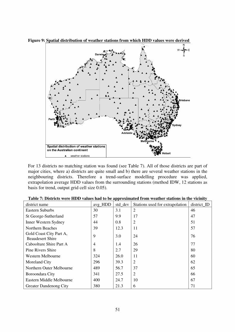
51

Figure 9: Spatial distribution of weather stations from which HDD values were derived

For 13 districts no matching station was found (see Table 7). All of those districts are part of major cities, where a) districts are quite small and b) there are several weather stations in the neighbouring districts. Therefore a trend-surface modelling procedure was applied, extrapolation average HDD values from the surrounding stations (method IDW, 12 stations as basis for trend, output grid cell size 0.05). Table 7: Districts were HDD values had to be approximated from weather stations in the vicinity

district name avg_HDD std_dev Stations used for extrapolation district_ID

Eastern Suburbs 30 3.1 2 46

St George-Sutherland 57 9.9 17 47

Inner Western Sydney 44 0.8 2 51

Northern Beaches 39 12.3 11 57

Gold Coast City Part A, Beaudesert Shire

9 3.0 24 76

Caboolture Shire Part A 4 1.4 26 77

Pine Rivers Shire 8 2.7 29 80

Western Melbourne 324 26.0 11 60

Moreland City 296 39.3 2 62

Northern Outer Melbourne 489 56.7 37 65

Boroondara City 341 27.5 2 66

Eastern Middle Melbourne 400 24.7 10 67

Greater Dandenong City 380 21.3 6 71

52

The final results of these procedures can be viewed in the methods section (Figure 6). As a comparison the official 30 years HDD average calculated by the Australian Bureau of Meteorology is presented in Figure 10. A comparison of both figures (Figure 6 and Figure 10) shows a good agreement between the 1999 values and the 30 year average. Figure 10: 30 year average of annual HDD from the Australian Bureau of Meterology

53

Appendix 4: Calculation Method for the Area-based Gini coefficients of Energy

Requirements

Gini coefficients were originally developed to quantify levels of income inequality in any given population. They are obtained from Lorenz curves, which plot the cumulative population fractions on the horizontal axis, sorted by the special per capita value of interest, with respect to cumulative fractions of interest on the vertical axis. The Gini coefficient then measures the Lorenz curve's deviation from the diagonal of perfect equality and ranges from zero to one, where zero indicates total equality and one total inequality. This measurement is usually applied to quantify income or wealth distributions in an economy. Goodman and Oldfield (2004) argued for the extension of the Gini coefficient to measure expenditure inequality, as it may reflect long-run differences in people’s circumstances much better than income, which can exhibit short term fluctuations. These are usually smoothed out by the use of savings – or more recently by increasing debt-based consumption (La Cava, Simon, 2005). Therefore focusing on expenditure inequalities can potentially mask long term trends in socio-economic inequalities (Druckman, Jackson, 2008c). Recently the Gini coefficient indicator has been modified to investigate “a wide variety of other kinds of area-based resource and associated emissions inequalities” (Druckman, Jackson, 2008b: S. 242). Various authors deployed Gini coefficients to investigate national inequalities in energy consumption at the household or at the per capita level (Herendeen 1974; Kok et al. 2003; Papathanasopoulou and Jackson 2009). Gini coefficients G are formally calculated as presented in (Equation 9. � = 1

2�² ∗ ���

���

��� − ��� (Equation 9)

where yi and yj are the incomes of the ith and jth household, � represents the average income and there are n households (Barr 1998). When the formula is adapted to calculate the AR-Gini coefficient, yi and yj represent the average amount of resources/energy/emissions used in the ith and jth district or region, n stands for the number of districts in the sample and � is the average resource use across all districts (Druckman and Jackson, 2008b). The empirical basis for the application presented by Druckman and Jackson (2008b) is the average resource use by districts, which are established on account of their socio-economic homogeneity. For the application in this study, only 85 rather large districts could be utilized (see appendix 2 for more details). This potentially decreases the absolute levels of inequality observable in this approach, because small pockets of very high / low levels of energy requirements could get lost in the process of aggregation and averaging. More detailed studies at several scales and different levels of spatial aggregation would be necessary to investigate the size of this effect. This goes beyond the scope of this study. Another important point raised in the literature relates to the fact that “it is possible to have two economies that have the same Gini coefficient but have different income distributions. [...] This ambiguity occurs when the Lorenz curves intersect” (Druckman, Jackson, 2008c: S. 244). When conducting a visual investigation of the Lorenz curves for energy requirements as well as income levels no case of intersection can be found. Therefore the application and interpretation of the AR-Gini is quite straightforward (see results chapter).

54

Figure 11: Area based Lorenz curves I

Figure 12: Area based Lorenz curves II

55

Appendix 5: The Household Expenditure Survey and Socio-Demographic Data –

preparing for statistical analysis

For the application of statistical methods, including multivariate regression analysis, socio-demographic information about the 85 districts of interest (appendix 1 and 2) is necessary. This data was supplied in the form of supplemental data (ABS, 2000), as well as census data (ABS, 2003). Based on previous work (Dey et al., 2007), these data sources were combined and prepared for statistical analysis. For this study, further data was added (HDD – see appendix 0). All statistical analysis presented in this work has undergone extensive model testing and statistical reliability checks (see methods section).

Appendix 6: Household Expenditure data by Australian and New Zealand

Standard Industry Classification (ANZSIC)

ISA-ID ANZSIC-ID ANZSIC-Abbrevation

Agriculture, Forestry, Fishing

1 0101000 She Sheep and lambs

2 0101001 Woo Shorn wool

3 0102000 Oat Oats, sorghum and other cereal grains

4 0102001 Wht Wheat

5 0102002 Bar Barley

6 0102003 Ric Rice

7 0102004 Osd Oilseeds

8 0102005 Leg Legumes

9 0103000 Bfc Beef cattle

10 0104000 Umk Untreated milk

11 0104001 Dyc Dairy cattle

12 0105000 Pig Pigs

13 0106000 Pty Poultry

14 0106001 Egg Eggs

15 0107000 Veg Vegetables

16 0107001 Frt Fruit

17 0107002 Nur Plant nurseries

18 0107003 Flo Flowers

19 0107004 Gra Grapes for wine

20 0107005 Hor Horses

21 0107006 Dee Deer

22 0107007 Pet Pet breeding

23 0107008 Suc Sugar cane

24 0107009 Cot Unginned cotton

25 0107010 Hop Hops

26 0107011 Grs Grass seed

27 0107012 Hay Hay

28 0107013 Rub Natural rubber

29 0200000 Skn Skins and other agricultural services

30 0200001 Ctg Ginned cotton

56

31 0200002 Cts Cotton seed

32 0200003 Shs Sheap shearing

33 0200004 Aea Aerial agriculture

34 0300000 Fop Other forest products

35 0300001 For Forestry

36 0300002 Swd Softwoods

37 0300003 Hwd Hardwoods

38 0400000 Ssq Services to fishing and squid jigging

39 0400001 Rlo Rock lobsters

40 0400002 Pra Prawns

41 0400003 Raf Raw fish

42 0400004 Oys Shellfish

43 0400005 Aqc Aquaculture

Mining

44 1100001 Blc Black coal

45 1100002 Brc Brown coal

46 1100003 Oil Crude oil

47 1100004 Ngs Natural gas

natural gas direct (energy content)

48 1100005 Lpg LPG, LNG

LPG; LNG direct (energy content)

49 1100006 Cog Other coal, oil and gas

50 1301000 Iro Iron ores

51 1302000 Nfo Other non-ferrous ores

52 1302001 Bxt Bauxite

53 1302002 Cop Copper concentrates and ores

54 1302003 Gol Gold

55 1302004 Ilm Ilmenite and Leucoxene

56 1302005 Rut Rutile

57 1302006 Msd Other mineral sands

58 1302007 Nic Nickel

59 1302008 Lea Lead

60 1302009 Siz Silver and zinc

61 1302010 Tin Tin

62 1302011 Urn Uranium

63 1302012 Man Manganese

64 1400000 Ggs Gemstones, gypsum, silica

65 1400001 Grv Gravel

66 1400002 San Sand

67 1400003 Dst Dimension stone

68 1400004 Cmt Construction materials nec

69 1400005 Lst Limestone

70 1400006 Cly Clays

71 1400007 Sal Salt

57

Manufacturing

74 2101000 Mep Meat products

75 2101001 Mea Fresh meat

76 2101002 Off Offal, hides, skins, blood meal

77 2101003 Pts Poultry, slaughtered

78 2102000 Dap Dairy products remainder

79 2102001 Tmk Treated milk

80 2102002 Chs Cheese

81 2102003 Bto Butter oil

82 2102004 But Butter

83 2103000 Vpr Vegetable products

84 2103001 Fpr Fruit products

85 2104000 Oif Oils and fats

86 2105000 Rip Rice products

87 2105001 Wfl Wheat flour

88 2105002 Fod Fodder and feed

89 2105003 Cer Flour mill products nec

90 2105004 Glt Gluten

91 2105005 Brf Breakfast foods

92 2105006 Flr Flour

93 2105007 Cak Cakes

94 2105009 Pas Pasta

95 2106000 Pcb Pies, cakes, biscuits

96 2106001 Brd Bread and bread rolls

97 2107000 Con Confectionery

98 2108000 Ofd Other food products

99 2108001 Rsg Raw sugar

100 2108002 Sug Refined sugar

101 2108003 Fis Fish

102 2108004 Lob Lobster

103 2108005 Sef Processed seafoods

104 2108006 Anf Animal food

105 2109000 Sfd Soft drinks

106 2110000 Bee Beer and malt

107 2111000 Spi Spirits

108 2111001 Win Wine

109 2112000 Tob Tobacco

110 2121000 Wsc Wool scouring

111 2122000 Hmf Human-made fibres

112 2123000 Cof Cotton fabrics

113 2124000 Wof Wool fabrics

114 2125000 Txf Textile finishing

115 2202000 Txp Textile products

116 2202001 Tcb Textile and canvas bags

117 2203000 Knm Knitting mill products

118 2204000 Clo Clothing

119 2205000 Ftw Footwear

58

120 2206000 Lth Leather products

121 2301000 Saw Sawmill products

122 2301001 Ust Undressed sawn timber

123 2301002 Scp Softwood woodchips

124 2301003 Rst Undressed resawn timber

125 2301004 Hcp Hardwood woodchips

126 2303000 Ppp Pulp, paper and paperboard

127 2311000 Mfw Manufactured wood

128 2312000 Joi Joinery products

129 2313000 Pac Paper containers

130 2314000 Pap Paper products

131 2401000 Prn Printing

132 2401001 Tad Trade advertising

133 2402000 Pub Recorded media and publishing nec

134 2402001 Nad Newspaper advertising

135 2402002 New Newspapers

136 2402003 Per Periodicals

137 2402004 Bok Books, maps, magazines

138 2501000 Pcp Petroleum and coal products

139 2501001 Ptr Petrol

Petrol direct (energy content)

140 2501002 Ker Kerosene

141 2501003 Gfo Gas oil or fuel oil

142 2501004 Bit Bitumen

143 2501005 Rlp Refinery LPG

144 2502000 Bcm Basic chemicals

145 2502001 Gas Gases

146 2503000 Pnt Paints

147 2504000 Pim Pesticides, insecticides and medicinal goods

148 2504001 Pha Pharmaceutical goods for human use

149 2505000 Sod Soap and other detergents

150 2506000 Cos Cosmetics and toiletry preparations

151 2507000 Chp Other chemical products

152 2507001 Exp Explosives and matches

153 2507002 Mun Munitions

154 2507003 Ink Inks

155 2507004 Glu Glue

156 2508000 Rup Rubber products

157 2508001 Tyr Tyres

158 2508002 Ret Retreading strips

159 2509000 Plp Plastic products

160 2511001 Sph Superphosphate

161 2511002 Mfe Mixed fertilisers

162 2511003 Cfe Other Chemical fertilisers

163 2601000 Glp Glass products

164 2602000 Crp Ceramic products

165 2603000 Cml Cement, lime

166 2603001 Rmc Ready-mixed concrete

59

167 2604000 Ccp Concrete products

168 2604001 Pls Plaster boards and plaster

169 2605000 Miw Other non-metallic mineral products

170 2605001 Stn Worked monumental or building stone

171 2605002 Glf Glass fibre and glass wool products

172 2605003 Gmn Ground minerals

173 2701000 Ist Iron and steel semi-manufactures

174 2702000 Nfs Non-ferrous non-aluminium semi-manufactures

175 2702001 Csl Copper, silver, lead, zinc

176 2702002 Ala Alumina

177 2702003 Alm Aluminium

178 2702004 Nik Nickel

179 2702005 Prm Precious metals

180 2702006 Als Aluminium semi-manufactures

181 2702007 Alf Aluminium foil

182 2703000 Stm Structural metal products

183 2703001 Fcs Fabricated construction steel

184 2703002 Rrd Reinforcing rods

185 2703003 Ald Aluminium doors

186 2703004 Aal Architectural aluminium

187 2703005 Smr Structural metal products repairing

188 2704000 Shm Sheet metal products

189 2705000 Fbm Fabricated metal products

190 2705001 Fir Firearms

191 2705002 Fmr Fabricated metal products repairing

192 2801000 Par Motor vehicle parts

193 2801001 Car Finished cars

194 2801002 Trk Trucks

195 2801003 Mvr Motor vehicle repairing

196 2802000 Shp Ships and boats

197 2802001 Sbr Ships and boat repairing

198 2803000 Rwy Railway equipment

199 2803001 Rwr Railway equipment repairing

200 2804000 Aic Aircraft

201 2804001 Acr Aircraft repairing

202 2805000 Pse Photographic and scientific equipment

203 2805001 Meq Surgical and medical

204 2805002 Sgl Spectacles and sunglasses

205 2806000 Enq Electronic equipment

206 2806001 Gam Gaming and vending machines

207 2807000 Hha Household appliances

208 2807001 Htg Space heaters, gas

209 2807002 Hte Space heaters, electric

210 2807003 Drf Domestic refrigerators

211 2807004 Rac Room air con

212 2807005 Crf Commercial refrigerators

213 2807006 Clw Clothes washing machines

214 2807007 Whs Water heater, solar

60

215 2807008 Whn Water heater, non-electric

216 2807009 Whe Water heater, electric

217 2808000 Elq Other electrical equipment

218 2809000 Cnm Construction machinery

219 2809001 Lif Hoists, cranes, lifting and loading machinery

220 2809002 Cgm Machinery for crushing, grinding, mixing

221 2809003 Drl Mining or drilling machinery and parts

222 2809004 Elv Elevators and escalators

223 2810000 Inm Industrial machinery and equipment

224 2810001 Pmp Pumps

225 2810002 Acn Air conditioning

226 2811001 Lwm Lawn mowers

227 2811002 Til Tillage, seeding, planting and fertilising equipment

228 2811003 Har Harvesting, haymaking and silage making equipment

229 2811004 Trc Agricultural tractors

230 2811005 Irr Irrigation equipment

231 2811006 Agm Agricultural machinery and parts nec

232 2901000 Pfb Prefabricated buildings

233 2902000 Fur Furniture

234 2902001 Wfn Wooden furniture

235 2902002 Mfn Sheet metal furniture

236 2902003 Mat Mattresses

237 2903000 Mmf Miscellaneous manufacturing

238 2903001 Jew Jewellerey

239 2903002 Sig Advertising signs

Electricity, Gas and Water Supply

240 3601000 Els Electricity supply

241 3602000 Gss Gas supply indirect

Gas supply direct (energy content)

242 3701000 Wts Water supply; sewerage and drainage services

Construction

243 4101000 Rsm Residential building repair and maintenance

244 4101001 Rsc Residential building construction

245 4102001 Nrc Non-residential building construction

246 4102002 Nrm Non-residential building repair and maintenance

247 4102003 Rdb Roads and bridges

248 4102004 Nbc Non-building construction

249 4102005 Nbm Non-building repair

Retail Trade

250 4501000 Wst Wholesale trade

251 5101000 Rtt Retail trade

252 5401000 Mlr Motor vehicle and lawn mower repairs

253 5401001 Imr Industrial machinery repairs

254 5402000 Bmr Business machines and equipment repairing and services

61

255 5402001 Wsr Wholesale repair and servicing

256 5402002 Hha Household elec applicances repair and service

257 5402003 Rtr Retail repair and service

Accommodation, Cafes and Restaurants

258 5701000 Hoc Hotels, clubs, restaurants and cafes

259 5701002 Acc Accommodation

Transport and Storage

260 6101000 Rdf Road freight

261 6101002 Bus Bus and tramway

262 6101003 Tax Taxi and hire car

263 6201001 Rwf Railway freight transport services

264 6201003 Rwp Railway passenger transport services

265 6201004 Ppt Pipeline transport

266 6201005 Tra Transport services nec

267 6301000 Wtt Water transport

268 6401000 Ast Air and space transport

269 6601001 Prk Parking services

270 6601002 Srd Services to road transport

271 6601003 Swt Services to water transport

272 6601006 Sai Services to air transport

273 6601007 Tag Travel and tourist agency services

274 6601008 Rff Road freight forwarding

275 6601009 Fwa Forwarding agencies

276 6601010 Cus Customs agencies

277 6601011 Sto Storage

Communication Services

278 7101000 Otc Overseas communication services and Pay TV

279 7101001 Pos Postal services

280 7101002 Cou Courier services

281 7101003 Dtc Domestic telecommunication services

Finance and Insurance

282 7301000 Bnk Banking

283 7302000 Nbk Non-bank finance

284 7401000 Ins Insurance

285 7401001 Lin Life insurance

286 7401002 Hin Health insurance

287 7401003 Pli Public liability

288 7501000 Sbd Security broking and dealing

289 7501001 Sfi Services to finance and investment

290 7501002 Sin Services to insurance

Property and Business Services

291 7701000 Odw Ownership of dwellings

62

292 7702000 Apb Other property services

293 7702001 Pod Property operator and developer services

294 7702003 Rea Real estate agent services

295 7702005 Mvh Motor vehicle hire

296 7702007 Plh Plant leasing, hiring and renting services

297 7801000 Coc Scientific research, technical and computer services

298 7801001 Res Research and meteorology services

299 7801002 Ars Architectural services

300 7801003 Svs Surveying services

301 7801004 Tcs Technical services nec

302 7801005 Dps Data processing services

303 7802001 Lgs Legal services

304 7802002 Acs Accounting services

305 7802003 Adv Advertising services

306 7802004 Mbs Market research and other business management services

307 7803001 Plc Employment placement

308 7803002 Tcm Typing, copying and mailing

309 7803003 Sec Security and investigation

310 7803004 Pcs Pest control

311 7803005 Cls Cleaning

312 7803006 Pak Packing

313 7803007 Cre Collecting and credit reporting

314 7803008 Bss Business services nec

Government Administration and Defence

315 8101000 Jud Judicial services

316 8101001 Fed Federal government

317 8101002 Sta State government

318 8101003 Loc Local government

319 8201000 Def Defence

Education

320 8401000 Edu Education

Health and Community Services

321 8601000 Hth GPs, dentists, optometrists, ambulance

322 8601001 Hos Hospitals and nursing homes

323 8601002 Chc Community health centres

324 8601003 Vet Veterinary services

Cultural and Recreational Services

325 9101000 Pic Motion pictures

326 9101001 Rtv Radio and television stations

327 9201001 Lib Library, museum and art gallery services

328 9201002 Pbz Parks, botanical gardens and zoos

329 9201003 Mus Music and theatre production

63

330 9201004 Art Creative arts

331 9201005 Nws News reporting

332 9201006 Ent Entertainment

333 9301001 Lot Lottery

334 9301002 Gmb Gambling

335 9301003 Tab TAB agencies

336 9301005 Spo Sport and recreation services (incl horse and dog racing, sports grounds, services)

Personal and Other Services

337 9501000 Psv Personal services

338 9501001 Phf Photographic film processing

339 9601001 Csr Community services and religious organisations

340 9601002 Int Interest groups and community organisations

341 9601003 Pol Police

342 9601004 Cor Corrective centres

343 9601005 Fbg Fire brigade

344 9601006 Gar Sanitary and garbage disposal

64

Appendix 7: Composition of energy requirement categories for statistical analysis

ISA-ID Total energy requirements

All categories

Direct energy requirements

47 Natural gas direct, indirect

48 LPG & LNG direct, indirect

139 Petrol direct, indirect

140 Kerosene

141 Gas oil or fuel oil

240 Electricity supply,

241 Gas supply direct, indirect

Indirect energy requirements

total - direct requirements

Private transportation requirements

48 LPG & LNG direct, indirect

139 Petrol direct, indirect

262 Taxi and hire car

Public transportation requirements

261 Bus and Tramway

264 Railway passenger

Residential direct requirements

47 Natural gas direct, indirect

240 Electricity supply,

241 Gas supply direct, indirect

Food related requirements (indirect)

1 Sheep and lambs

2 Shorn wool

3 Oats, sorghum and other cereal grains

4 Wheat

5 Barley

6 Rice

7 Oilseeds

8 Legumes

9 Beef cattle

10 Untreated milk

11 Dairy cattle

12 Pigs

13 Poultry

14 Eggs

15 Vegetables

16 Fruit

19 Grapes for wine

65

21 Deer

23 Sugar cane

25 Hops

39 Rock lobsters

40 Prawns

41 Raw fish

42 Shellfish

43 Aquaculture

74 Meat products

75 Fresh meat

76 Offal, hides, skins, blood meal

77 Poultry, slaughtered

78 Dairy products remainder

79 Treated milk

80 Cheese

81 Butter oil

82 Butter

83 Vegetable products

84 Fruit products

85 Oils and fats

86 Rice products

87 Wheat flour

88 Fodder and feed

89 Flour mill products nec

90 Gluten

91 Breakfast foods

92 Flour

93 Cakes

94 Pasta

95 Pies, cakes, biscuits

96 Bread and bread rolls

97 Confectionery

98 Other food products

99 Raw sugar

100 Refined sugar

101 Fish

102 Lobster

103 Processed seafoods

104 Animal food

105 Soft drinks

106 Beer and malt

107 Spirits

108 Wine

WORKING PAPERS SOCIAL ECOLOGY

Band 1 Umweltbelastungen in Österreich als Folge mensch-lichen Handelns. Forschungsbericht gem. m. dem Öster-reichischen Ökologie-Institut. Fischer-Kowalski, M., Hg. (1987) Band 2 Environmental Policy as an Interplay of Professionals and Movements - the Case of Austria. Paper to the ISA Conference on Environmental Constraints and Opportu-nities in the Social Organisation of Space, Udine 1989. Fischer-Kowalski, M. (1989) Band 3 Umwelt &Öffentlichkeit. Dokumentation der gleichnami-gen Tagung, veranstaltet vom IFF und dem Österreichi-schen Ökologie-Institut in Wien, (1990) Band 4 Umweltpolitik auf Gemeindeebene. Politikbezogene Weiterbildung für Umweltgemeinderäte. Lackner, C. (1990) Band 5 Verursacher von Umweltbelastungen. Grundsätzliche Überlegungen zu einem mit der VGR verknüpfbaren Emittenteninformationssystem. Fischer-Kowalski, M., Kisser, M., Payer, H., Steurer A. (1990) Band 6 Umweltbildung in Österreich, Teil I: Volkshochschulen. Fischer-Kowalski, M., Fröhlich, U.; Harauer, R., Vymazal R. (1990) Band 7 Amtliche Umweltberichterstattung in Österreich. Fischer-Kowalski, M., Lackner, C., Steurer, A. (1990) Band 8 Verursacherbezogene Umweltinformationen. Bausteine für ein Satellitensystem zur österr. VGR. Dokumentation des gleichnamigen Workshop, veranstaltet vom IFF und dem Österreichischen Ökologie-Institut, Wien (1991) Band 9 A Model for the Linkage between Economy and Envi-ronment. Paper to the Special IARIW Conference on Environmental Accounting, Baden 1991. Dell'Mour, R., Fleissner, P. , Hofkirchner, W.,; Steurer A. (1991) Band 10 Verursacherbezogene Umweltindikatoren - Kurzfassung. Forschungsbericht gem. mit dem Österreichischen Öko-logie-Institut. Fischer-Kowalski, M., Haberl, H., Payer, H.; Steurer, A., Zangerl-Weisz, H. (1991) Band 11 Gezielte Eingriffe in Lebensprozesse. Vorschlag für verursacherbezogene Umweltindikatoren. For-schungsbericht gem. m. dem Österreichischen Ökologie-Institut. Haberl, H. (1991) Band 12 Gentechnik als gezielter Eingriff in Lebensprozesse. Vorüberlegungen für verursacherbezogene Umweltindi-katoren. Forschungsbericht gem. m. dem Österr. Ökolo-gie-Institut. Wenzl, P.; Zangerl-Weisz, H. (1991)

Band 13 Transportintensität und Emissionen. Beschreibung ös-terr. Wirtschaftssektoren mittels Input-Output-Mo-dellierung. Forschungsbericht gem. m. dem Österr. Öko-logie-Institut. Dell'Mour, R.; Fleissner, P.; Hofkirchner, W.; Steurer, A. (1991) Band 14 Indikatoren für die Materialintensität der österreichischen Wirtschaft. Forschungsbericht gem. m. dem Österreichi-schen Ökologie-Institut. Payer, H. unter Mitarbeit von K. Turetschek (1991) Band 15 Die Emissionen der österreichischen Wirtschaft. Syste-matik und Ermittelbarkeit. Forschungsbericht gem. m. dem Österr. Ökologie-Institut. Payer, H.; Zangerl-Weisz, H. unter Mitarbeit von R.Fellinger (1991) Band 16 Umwelt als Thema der allgemeinen und politischen Er-wachsenenbildung in Österreich. Fischer-Kowalski M., Fröhlich, U.; Harauer, R.; Vymazal, R. (1991) Band 17 Causer related environmental indicators - A contribution to the environmental satellite-system of the Austrian SNA. Paper for the Special IARIW Conference on Envi-ronmental Accounting, Baden 1991. Fischer-Kowalski, M., Haberl, H., Payer, H., Steurer, A. (1991) Band 18 Emissions and Purposive Interventions into Life Pro-cesses - Indicators for the Austrian Environmental Ac-counting System. Paper to the ÖGBPT Workshop on Ecologic Bioprocessing, Graz 1991. Fischer-Kowalski M., Haberl, H., Wenzl, P., Zangerl-Weisz, H. (1991) Band 19 Defensivkosten zugunsten des Waldes in Österreich. Forschungsbericht gem. m. dem Österreichischen Insti-tut für Wirtschaftsforschung. Fischer-Kowalski et al. (1991) Band 20* Basisdaten für ein Input/Output-Modell zur Kopplung ökonomischer Daten mit Emissionsdaten für den Bereich des Straßenverkehrs. Steurer, A. (1991) Band 22 A Paradise for Paradigms - Outlining an Information System on Physical Exchanges between the Economy and Nature. Fischer-Kowalski, M., Haberl, H., Payer, H. (1992) Band 23 Purposive Interventions into Life-Processes - An Attempt to Describe the Structural Dimensions of the Man-Animal-Relationship. Paper to the Internat. Conference on "Science and the Human-Animal-Relationship", Am-sterdam 1992. Fischer-Kowalski, M., Haberl, H. (1992) Band 24 Purposive Interventions into Life Processes: A Neglected "Environmental" Dimension of the Society-Nature Rela-tionship. Paper to the 1. Europ. Conference of Sociology, Vienna 1992. Fischer-Kowalski, M., Haberl, H. (1992)

WORKING PAPERS SOCIAL ECOLOGY

Band 25 Informationsgrundlagen struktureller Ökologisierung. Beitrag zur Tagung "Strategien der Kreislaufwirtschaft: Ganzheitl. Umweltschutz/Integrated Environmental Pro-tection", Graz 1992. Steurer, A., Fischer-Kowalski, M. (1992) Band 26 Stoffstrombilanz Österreich 1988. Steurer, A. (1992) Band 28 Naturschutzaufwendungen in Österreich. Gutachten für den WWF Österreich. Payer, H. (1992) Band 29 Indikatoren der Nachhaltigkeit für die Volkswirt-schaftliche Gesamtrechnung - angewandt auf die Region. Payer, H. (1992). In: KudlMudl SonderNr. 1992:Tagungsbericht über das Dorfsymposium "Zukunft der Region - Region der Zukunft?" Band 31 Leerzeichen. Neuere Texte zur Anthropologie. Macho, T. (1993) Band 32 Metabolism and Colonisation. Modes of Production and the Physical Exchange between Societies and Nature. Fischer-Kowalski, M., Haberl, H. (1993) Band 33 Theoretische Überlegungen zur ökologischen Bedeutung der menschlichen Aneignung von Nettoprimärprodukti-on. Haberl, H. (1993) Band 34 Stoffstrombilanz Österreich 1970-1990 - Inputseite. Steu-rer, A. (1994) Band 35 Der Gesamtenergieinput des Sozio-ökonomischen Sys-tems in Österreich 1960-1991. Zur Erweiterung des Be-griffes "Energieverbrauch". Haberl, H. (1994) Band 36 Ökologie und Sozialpolitik. Fischer-Kowalski, M. (1994) Band 37 Stoffströme der Chemieproduktion 1970-1990. Payer, H., unter Mitarbeit von Zangerl-Weisz, H. und Fellinger, R. (1994) Band 38 Wasser und Wirtschaftswachstum. Untersuchung von Abhängigkeiten und Entkoppelungen, Wasserbilanz Österreich 1991. Hüttler, W., Payer, H. unter Mitarbeit von H. Schandl (1994) Band 39 Politische Jahreszeiten. 12 Beiträge zur politischen Wen-de 1989 in Ostmitteleuropa. Macho, T. (1994) Band 40 On the Cultural Evolution of Social Metabolism with Nature. Sustainability Problems Quantified. Fischer-Kowalski, M., Haberl, H. (1994) Band 41 Weiterbildungslehrgänge für das Berufsfeld ökologischer Beratung. Erhebung u. Einschätzung der Angebote in Österreich sowie von ausgewählten Beispielen in Deutschland, der Schweiz, Frankreich, England und europaweiten Lehrgängen. Rauch, F. (1994)

Band 42 Soziale Anforderungen an eine nachhaltige Entwicklung. Fischer-Kowalski, M., Madlener, R., Payer, H., Pfeffer, T., Schandl, H. (1995) Band 43 Menschliche Eingriffe in den natürlichen Energiefluß von Ökosystemen. Sozio-ökonomische Aneignung von Nettoprimär-produktion in den Bezirken Österreichs. Haberl, H. (1995) Band 44 Materialfluß Österreich 1990. Hüttler, W., Payer, H.; Schandl, H. (1996) Band 45 National Material Flow Analysis for Austria 1992. Socie-ty’s Metabolism and Sustainable Development. Hüttler, W. Payer, H., Schandl, H. (1997) Band 46 Society’s Metabolism. On the Development of Concepts and Methodology of Material Flow Analysis. A Review of the Literature. Fischer-Kowalski, M. (1997) Band 47 Materialbilanz Chemie-Methodik sektoraler Materialbilan-zen. Schandl, H., Weisz, H. Wien (1997) Band 48 Physical Flows and Moral Positions. An Essay in Memory of Wildavsky. A. Thompson, M. (1997) Band 49 Stoffwechsel in einem indischen Dorf. Fallstudie Merkar. Mehta, L., Winiwarter, V. (1997) Band 50+ Materialfluß Österreich- die materielle Basis der Österrei-chischen Gesellschaft im Zeitraum 1960-1995. Schandl, H. (1998) Band 51+ Bodenfruchtbarkeit und Schädlinge im Kontext von Ag-rargesellschaften. Dirlinger, H., Fliegenschnee, M., Kraus-mann, F., Liska, G., Schmid, M. A. (1997) Band 52+ Der Naturbegriff und das Gesellschaft-Natur-Verhältnis in der frühen Soziologie. Lutz, J. Wien (1998) Band 53+ NEMO: Entwicklungsprogramm für ein Nationales Emis-sionsmonitoring. Bruckner, W., Fischer-Kowalski, M., Jorde, T. (1998) Band 54+ Was ist Umweltgeschichte? Winiwarter, V. (1998)

Mit + gekennzeichnete Bände sind unter http://www.uni-klu.ac.at/socec/inhalt/1818.htm

Im PDF-Format downloadbar.

WORKING PAPERS SOCIAL ECOLOGY

Band 55+ Agrarische Produktion als Interaktion von Natur und Gesellschaft: Fallstudie SangSaeng. Grünbühel, C. M., Schandl, H., Winiwarter, V. (1999) Band 57+ Colonizing Landscapes: Human Appropriation of Net Primary Production and its Influence on Standing Crop and Biomass Turnover in Austria. Haberl, H., Erb, K.H., Krausmann, F., Loibl, W., Schulz, N. B., Weisz, H. (1999) Band 58+ Die Beeinflussung des oberirdischen Standing Crop und Turnover in Österreich durch die menschliche Gesell-schaft. Erb, K. H. (1999) Band 59+ Das Leitbild "Nachhaltige Stadt". Astleithner, F. (1999) Band 60+ Materialflüsse im Krankenhaus, Entwicklung einer Input-Output Methodik. Weisz, B. U. (2001) Band 61+ Metabolismus der Privathaushalte am Beispiel Öster-reichs. Hutter, D. (2001) Band 62+ Der ökologische Fußabdruck des österreichischen Au-ßenhandels. Erb, K.H., Krausmann, F., Schulz, N. B. (2002) Band 63+ Material Flow Accounting in Amazonia: A Tool for Sus-tainable Development. Amann, C., Bruckner, W., Fischer-Kowalski, M., Grünbühel, C. M. (2002) Band 64+ Energieflüsse im österreichischen Landwirtschaftssektor 1950-1995, Eine humanökologische Untersuchung. Dar-ge, E. (2002) Band 65+ Biomasseeinsatz und Landnutzung Österreich 1995-2020. Haberl, H.; Krausmann, F.; Erb, K.H.;Schulz, N. B.; Adensam, H. (2002) Band 66+ Der Einfluss des Menschen auf die Artenvielfalt. Gesell-schaftliche Aneignung von Nettoprimärproduktion als

Pressure-Indikator für den Verlust von Biodiversität. Haberl, H., Fischer-Kowalski, M., Schulz, N. B., Plutzar, C., Erb, K.H., Krausmann, F., Loibl, W., Weisz, H.; Sauberer, N., Pollheimer, M. (2002)

Band 67+ Materialflussrechnung London. Bongardt, B. (2002) Band 68+ Gesellschaftliche Stickstoffflüsse des österreichischen Landwirtschaftssektors 1950-1995, Eine humanökologi-sche Untersuchung. Gaube, V. (2002) Band 69+ The transformation of society's natural relations: from the agrarian to the industrial system. Research strategy for an empirically informed approach towards a Europe-an Environmental History. Fischer-Kowalski, M., Krausmann, F., Schandl, H. (2003) Band 70+ Long Term Industrial Transformation: A Comparative Study on the Development of Social Metabolism and Land Use in Austria and the United Kingdom 1830-2000. Krausmann, F., Schandl, H., Schulz, N. B. (2003)

Band 72+ Land Use and Socio-economic Metabolism in Pre-industrial Agricultural Systems: Four Nineteenth-century Austrain Villages in Comparison. Krausmann, F. (2008)

Band 73+ Handbook of Physical Accounting Measuring bio-physical dimensions of socio-economic activities MFA – EFA – HANPP. Schandl, H., Grünbühel, C. M., Haberl, H., Weisz, H. (2004) Band 74+ Materialflüsse in den USA, Saudi Arabien und der Schweiz. Eisenmenger, N.; Kratochvil, R.; Krausmann, F.; Baart, I.; Colard, A.; Ehgartner, Ch.; Eichinger, M.; Hempel, G.; Lehrner, A.; Müllauer, R.; Nourbakhch-Sabet, R.; Paler, M.; Patsch, B.; Rieder, F.; Schembera, E.; Schieder, W.; Schmiedl, C.; Schwarzlmüller, E.; Stadler, W.; Wirl, C.; Zandl, S.; Zika, M. (2005) Band 75+ Towards a model predicting freight transport from mate-rial flows. Fischer-Kowalski, M. (2004) Band 76+ The physical economy of the European Union: Cross-country comparison and determinants of material con-sumption. Weisz, H., Krausmann, F., Amann, Ch., Eisen-menger, N., Erb, K.H., Hubacek, K., Fischer-Kowalski, M. (2005) Band 77+ Arbeitszeit und Nachhaltige Entwicklung in Europa: Ausgleich von Produktivitätsgewinn in Zeit statt Geld? Proinger, J. (2005) Band 78+ Sozial-Ökologische Charakteristika von Agrarsystemen. Ein globaler Überblick und Vergleich. Lauk, C. (2005) Band 79+ Verbrauchsorientierte Abrechnung von Wasser als Wa-ter-Demand-Management-Strategie. Eine Analyse anhand eines Vergleichs zwischen Wien und Barcelona. Machold, P. (2005) Band 80+ Ecology, Rituals and System-Dynamics. An attempt to model the Socio-Ecological System of Trinket Island. Wildenberg, M. (2005) Band 81+ Southeast Asia in Transition. Socio-economic transi-tions, environmental impact and sustainable develop-ment. Fischer-Kowalski, M., Schandl, H., Grünbühel, C., Haas, W., Erb, K-H., Weisz, H., Haberl, H. (2004) Helmut Haberl Band 83+ HANPP-relevante Charakteristika von Wanderfeldbau und anderen Langbrachesystemen. Lauk, C. (2006) Band 84+ Management unternehmerischer Nachhaltigkeit mit Hilfe der Sustainability Balanced Scorecard. Zeitlhofer, M. (2006) Band 85+ Nicht-nachhaltige Trends in Österreich: Maßnahmenvor-schläge zum Ressourceneinsatz. Haberl, H., Jasch, C., Adensam, H., Gaube, V. (2006) Band 87+ Accounting for raw material equivalents of traded goods. A comparison of input-output approaches in physical, monetary, and mixed units. Weisz, H. (2006)

WORKING PAPERS SOCIAL ECOLOGY

Band 88+ Vom Materialfluss zum Gütertransport. Eine Analyse anhand der EU15 – Länder (1970-2000). Rainer, G. (2006) Band 89+ Nutzen der MFA für das Treibhausgas-Monitoring im Rahmen eines Full Carbon Accounting-Ansatzes; Feasi-bilitystudie; Endbericht zum Projekt BMLFUW-UW.1.4.18/0046-V/10/2005. Erb, K.-H., Kastner, T., Zandl, S., Weisz, H., Haberl, H., Jonas, M., (2006) Band 90+ Local Material Flow Analysis in Social Context in Tat Hamelt, Northern Mountain Region, Vietnam. Hobbes, M.; Kleijn, R. (2006) Band 91+ Auswirkungen des thailändischen logging ban auf die Wälder von Laos. Hirsch, H. (2006) Band 92+ Human appropriation of net primary produktion (HANPP) in the Philippines 1910-2003: a socio-ecological analysis. Kastner, T. (2007) Band 93+ Landnutzung und landwirtschaftliche Entscheidungs-strukturen. Partizipative Entwicklung von Szenarien für das Traisental mit Hilfe eines agentenbasierten Modells. Adensam, H., V. Gaube, H. Haberl, J. Lutz, H. Reisinger, J. Breinesberger, A. Colard, B. Aigner, R. Maier, Punz, W. (2007) Band 94+ The Work of Konstantin G. Gofman and colleagues: An early example of Material Flow Analysis from the Soviet Union. Fischer-Kowalski, M.; Wien (2007) Band 95+ Partizipative Modellbildung, Akteurs- und Ökosystemana-lyse in Agrarintensivregionen; Schlußbericht des deutsch-österreichischen Verbundprojektes. Newig, J., Gaube, V., Berkhoff, K., Kaldrack, K., Kastens, B., Lutz, J., Schlußmeier B., Adensam, H., Haberl, H., Pahl-Wostl, C., Colard, A., Aigner, B., Maier, R., Punz, W.; Wien (2007) Band 96+ Rekonstruktion der Arbeitszeit in der Landwirtschaft im 19. Jahrhundert am Beispiel von Theyern in Nie-derösterreich. Schaschl, E.; Wien (2007) Band 98+ Local Material Flow Analysis in Social Context at the forest fringe in the Sierra Madre, the Philippines. Hobbes, M., Kleijn, R. (Hrsg); Wien (2007) Band 99+ Human Appropriation of Net Primary Production (HANPP) in Spain, 1955-2003: A socio-ecological analysis. Schwarzlmüller, E.; Wien (2008) Band 100+ Scaling issues in long-term socio-ecological biodi-versity research: A review of European cases. Dirn-böck, T., Bezák, P., Dullinger S., Haberl, H., Lotze-Campen, H., Mirtl, M., Peterseil, J., Redpath, S., Singh, S., Travis, J., Wijdeven, S.M.J.; Wien (2008)

Band 101+ Human Appropriation of Net Primary Production (HANPP) in the United Kingdom, 1800-2000: A socio-ecological analysis. Musel, A.; Wien (2008) Band 102 + Wie kann Wissenschaft gesellschaftliche Verände-rung bewirken? Eine Hommage an Alvin Gouldner, und ein Versuch, mit seinen Mitteln heutige Klima-politik zu verstehen. Fischer-Kowalski, M.; Wien (2008) Band 103+ Sozialökologische Dimensionen der österreichischen Ernährung – Eine Szenarienanalyse. Lackner, M.; Wien (2008) Band 104+ Fundamentals of Complex Evolving Systems: A Primer. Weis, E.; Wien (2008) Band 105+ Umweltpolitische Prozesse aus diskurstheoretischer Perspektive: Eine Analyse des Südtiroler Feinstaubprob-lems von der Problemkonstruktion bis zur Umsetzung von Regulierungsmaßnahmen. Paler, M.; Wien (2008) Band 106+ Ein integriertes Modell für Reichraming. Partizipative Entwicklung von Szenarien für die Gemeinde Reich-raming (Eisenwurzen) mit Hilfe eines agentenbasierten Landnutzungsmodells. Gaube, V., Kaiser, C., Widenberg, M., Adensam, H., Fleissner, P., Kobler, J., Lutz, J., Smetschka, B., Wolf, A., Richter, A., Haberl, H.; Wien (2008) Band 107+ Der soziale Metabolismus lokaler Produktionssysteme: Reichraming in der oberösterreichischen Eisenwurzen 1830-2000. Gingrich, S., Krausmann, F.; Wien (2008) Band 108+ Akteursanalyse zum besseren Verständnis der Entwick-lungsoptionen von Bioenergie in Reichraming. Eine sozialökologische Studie. Vrzak, E.; Wien (2008) Band 109+ Direktvermarktung in Reichraming aus sozial-ökologischer Perspektive. Zeitlhofer, M.; Wien (2008) Band 110+ CO2-Bilanz der Tomatenproduktion: Analyse acht ver-schiedener Produktionssysteme in Österreich, Spanien und Italien. Theurl, M.; Wien (2008) Band 111+ Die Rolle von Arbeitszeit und Einkommen bei Rebound-Effekten in Dematerialisierungs- und Dekarbonisierungs-strategien. Eine Literaturstudie. Bruckner, M.; Wien (2008) Band 112+ Von Kommunikation zu materiellen Effekten - Ansatzpunkte für eine sozial-ökologische Lesart von Luhmanns Theorie Sozialer Systeme. Rieder, F.; Wien (2008) Band 113+ (in Vorbereitung)

WORKING PAPERS SOCIAL ECOLOGY

Band 114+ Across a Moving Threshold: energy, carbon and the efficiency of meeting global human development needs. Steinberger, J. K., Roberts, .J.T.; Wien (2008) Band 115 Towards a low carbon society: Setting targets for a re-duction of global resource use. Krausmann, F., Fischer-Kowalski, M., Steinberger, J.K., Ayres, R.U.; Wien (2010) Band 116+ Eating the Planet: Feeding and fuelling the world sus-tainably, fairly and humanely - a scoping study. Erb, K-H., Haberl, H., Krausmann, F., Lauk, C., Plutzar, C., Steinberger, J.K., Müller, C., Bondeau, A., Waha, K., Pollack, G.; Wien (2009) Band 117+ Gesellschaftliche Naturverhältnisse: Energiequellen und die globale Transformation des gesellschaftlichen Stoff-wechsels. Krausmann, F., Fischer-Kowalski, M.; Wien (2010) Band 118+ Zurück zur Fläche? Eine Untersuchung der biophysi-schen Ökonomie Brasiliens zwischen 1970 und 2005. Mayer, A.; Wien (2010) Band 119+ Das nachhaltige Krankenhaus: Erprobungsphase. Weisz, U., Haas, W., Pelikan, J.M., Schmied, H., Himpelmann, M., Purzner, K., Hartl, S., David, H.; Wien (2009) Band 120+ LOCAL STUDIES MANUAL A researcher’s guide for investigating the social metabolism of local rural systems. Singh, S.J., Ringhofer, L., Haas, W., Krausmann, F., Fischer-Kowalski, M.; Wien (2010) Band 121+ Sociometabolic regimes in indigenous communities and the crucial role of working time: A comparison of case studies. Fischer-Kowalski, M., Singh, S.J., Ringhofer, L., Grünbühel C.M., Lauk, C., Remesch., A.; Wien (2010) Band 122+ Klimapolitik im Bereich Gebäude und Raumwärme. Entwicklung, Problemfelder und Instrumente der Länder Österreich, Deutschland und Schweiz. Jöbstl, R.; Wien (2010) Band 123+ Trends and Developments of the Use of Natural Re-sources in the European Union. Krausmann, F., Fischer-Kowalski, M., Steinberger, J.K., Schaffartzik, A., Eisenmenger, N, Weisz, U.; Wien (2011) Band 126+ Masterstudium "Sozial- und Humanökologie": Selbstevaluation 2005-2010. Schmid, M., Mayer A., Miechtner, G.; Wien (2010) Band 127 + Bericht des Zentrums für Evaluation und Forschungsbe-ratung (ZEF). Das Masterstudium „Sozial- und Human-ökologie“. Mayring, P., Fenzl, T.; Wien (2010)

Band 128+ Die langfristigen Trends der Material- und Energieflüsse in den USA in den Jahren 1850 bis 2005. Gierlinger, S.; Wien (2010)

Band 129+ Die Verzehrungssteuer 1829 – 1913 als Grundlage einer umwelthistorischen Untersuchung des Metabolismus der Stadt Wien. Hauer, F.; Wien (2010)

Band 130+ Human Appropriation of Net Primary Production in South Africa, 1961- 2006. A socio-ecological analysis. Niedertscheider, M.; Wien (2011) Band 131+ The socio-metabolic transition. Long term historical trends and patterns in global mate-rial and energy use. Krausmann, F. (Editor); Wien (2011) Band 132 „Urlaub am Bauernhof“ oder „Bauernhof ohne Urlaub“? Eine sozial-ökologische Untersuchung der geschlechts-spezifischen Arbeitsteilung und Zeitverwendung auf landwirtschaftlichen Betrieben in der Gemeinde Andels-buch, Bregenzerwald. Winder, M.; Wien (2011) Band 133 Spatial and Socio-economic Drivers of Direct and Indirect Household Energy Consumption in Australia Wiedenhofer, D.; Wien (2011)