Sparse Latent Semantic Analysis

Xi Chen∗ Yanjun Qi † Bing Bai† Qihang Lin ‡ Jaime G. Carbonell§

Abstract

Latent semantic analysis (LSA), as one of the most pop-ular unsupervised dimension reduction tools, has a widerange of applications in text mining and information re-trieval. The key idea of LSA is to learn a projectionmatrix that maps the high dimensional vector spacerepresentations of documents to a lower dimensional la-tent space, i.e. so called latent topic space. In this pa-per, we propose a new model called Sparse LSA, whichproduces a sparse projection matrix via the `1 regu-larization. Compared to the traditional LSA, SparseLSA selects only a small number of relevant words foreach topic and hence provides a compact representationof topic-word relationships. Moreover, Sparse LSA iscomputationally very efficient with much less memoryusage for storing the projection matrix. Furthermore,we propose two important extensions of Sparse LSA:group structured Sparse LSA and non-negative SparseLSA. We conduct experiments on several benchmarkdatasets and compare Sparse LSA and its extensionswith several widely used methods, e.g. LSA, SparseCoding and LDA. Empirical results suggest that SparseLSA achieves similar performance gains to LSA, but ismore efficient in projection computation, storage, andalso well explain the topic-word relationships.

1 Introduction

Latent Semantic Analysis (LSA) [5], as one of the mostsuccessful tools for learning the concepts or latent topicsfrom text, has widely been used for the dimension reduc-tion purpose in information retrieval. More precisely,given a document-term matrix X ∈ RN×M , where Nis the number of documents and M is the number ofwords, and assuming that the number of latent top-ics (the dimensionality of the latent space) is set asD (D ≤ min{N,M}), LSA applies singular value de-composition (SVD) to construct a low rank (with rank-D) approximation of X: X ≈ USVT , where the col-umn orthogonal matrices U ∈ RN×D (UTU = I) andV ∈ RM×D (VTV = I) represent document and word

∗Machine Learning Department, Carnegie Mellon University†NEC Lab America‡Tepper School of Business, Carnegie Mellon University§Language Technology Institute, Carnegie Mellon University

embeddings into the latent space. S is a diagonal ma-trix with the D largest singular values of X on the di-agonal 1. Subsequently, the so-called projection matrixdefined as A = S−1VT provides a transformation map-ping of documents from the word space to the latenttopic space, which is less noisy and considers word syn-onymy (i.e. different words describing the same idea).However, in LSA, each latent topic is represented byall word features which sometimes makes it difficult toprecisely characterize the topic-word relationships.

In this paper, we introduce a scalable latent topicmodel that we call “Sparse Latent Semantic Analysis”(Sparse LSA). Different from the traditional LSA basedon SVD, we formulate a variant of LSA as an optimiza-tion problem which minimizes the approximation errorunder the orthogonality constraint of U. Based on thisformulation, we add the sparsity constraint of the pro-jection matrix A via the `1 regularization as in the lassomodel [23]. By enforcing the sparsity on A, the modelhas the ability to automatically select the most relevantwords for each latent topic. There are several importantfeatures of Sparse LSA model:

1. It is intuitive that only a part of the vocabulary canbe relevant to a certain topic. By enforcing sparsityof A such that each row (representing a latenttopic) only has a small number nonzero entries(representing the most relevant words), Sparse LSAcan provide us a compact representation for topic-word relationship that is easier to interpret.

2. With the adjustment of sparsity level in projectionmatrix, we could control the granularity (“level-of-details”) of the topics we are trying to discover,e.g. more generic topics have more nonzero entriesin rows of A than specific topics.

3. Due to the sparsity of A, Sparse LSA providesan efficient strategy both in the time cost of theprojection operation and in the storage cost of theprojection matrix when the dimensionality of latentspace D is large.

1Since it is easier to explain our Sparse LSA model in terms ofdocument-term matrix, for the purpose of consistency, we intro-duce SVD based on the document-term matrix which is differentfrom standard notations using the term-document matrix.

4. Sparse LSA could project a document q into asparse vector representation q where each entry ofq corresponds to a latent topic. In other words,we could know the topics that q belongs to directlyform the position of nonzero entries of q. Moreover,sparse representation of projected documents willsave a lot of computational cost for the subsequentretrieval tasks, e.g. ranking (considering computingcosine similarity), text categorization, etc.

Furthermore, we propose two important extensionsbased on Sparse LSA:

1. Group Structured Sparse LSA: we add group struc-tured sparsity-inducing penalty as in [24] to selectthe most relevant groups of features relevant to thelatent topic.

2. Non-negative Sparse LSA: we further enforce thenon-negativity constraint on the projection matrixA. It could provide us a pseudo probabilitydistribution of each word given the topic, similaras in Latent Dirichlet Allocation (LDA) [3].

We conduct experiments on four benchmark datasets, with two on text categorization, one on breastcancer gene function identification, and the last oneon topic-word relationship identification from NIPSproceeding papers. We compare Sparse LSA and itsvariants with several popular methods, e.g. LSA [5],Sparse Coding [16] and LDA [3]. Empirical resultsshow clear advantages of our methods in terms ofcomputational cost, storage and the ability to generatesensible topics and to select relevant words (or genes)for the latent topics.

The rest of this paper is as follows. In Section 2, wepresent the basic Sparse LSA model. In Section 3, weextend Sparse LSA to group structured Sparse LSA andnon-negative Sparse LSA. Related work is discussed inSection 4 and the empirical evaluation of the models isin Section 5. We conclude the paper in Section 6.

2 Sparse LSA

2.1 Optimization Formulation of LSA We con-sider N documents, where each document lies in an M -dimensional feature space X , e.g. tf-idf [1] weights of thevocabulary with the normalization to unit length. Wedenote N documents by a matrix X = [X1, . . . , XM ] ∈RN×M , where Xj ∈ RN is the j-th feature vector for allthe documents. For the dimension reduction purpose,we aim to derive a mapping that projects input fea-ture space into a D-dimensional latent space where Dis smaller than M . In the information retrieval content,each latent dimension is also called an hidden “topic”.

Motivated by the latent factor analysis [9], weassume that we have D uncorrelated latent variablesU1, . . . , UD, where each Ud ∈ RN has the unit length,i.e. ‖Ud‖2 = 1. Here ‖ · ‖2 denotes the vector `2-norm.For the notation simplicity, we put latent variablesU1, . . . , UD into a matrix: U = [U1, . . . , UD] ∈ RN×D.Since latent variables are uncorrelated with the unitlength, we have UTU = I, where I is the identitymatrix. We also assume that each feature vector Xj canbe represented as a linear expansion in latent variablesU1, . . . , UD:

(2.1) Xj =D∑

d=1

adjUd + εj ,

or simply X = UA + ε, where A = [adj ] ∈ RD×Mgives the mapping from the latent space to the inputfeature space and ε is the zero mean noise. Our goal isto compute the so-called projection matrix A.

We can achieve this by solving the following opti-mization problem which minimizes the rank-D approx-imation error subject to the orthogonality constraint ofU:

minU,A12‖X−UA‖2F(2.2)

subject to: UTU = I,

where ‖ · ‖F denotes the matrix Frobenius norm. Theconstraint UTU = I is according to the uncorrelatedproperty among latent variables.

At the optimum of Eq. (2.2), UA leads to the bestrank-D approximation of the data X. In general, largerthe D is, the better the reconstruction performance.However, larger D requires more computational costand large amount memory for storing A. This is theissue that we will address in the next section.

After obtaining A, given a new document q ∈ RM ,its representation in the lower dimensional latent spacecan be computed as:

(2.3) q = Aq.

2.2 Sparse LSA As discussed in the introduction,one notable advantage of sparse LSA is due to itsgood interpretability in topic-word relationship. SparseLSA automatically selects the most relevant words foreach latent topic and hence provides us a clear andcompact representation of the topic-word relationship.Moreover, for a new document q, if the words in q hasno intersection with the relevant words of d-th topic(nonzero entries in Ad, the d-th row of A), the d-thelement of q, Adq, will become zero. In other words,the sparse latent representation of q clearly indicatesthe topics that q belongs to.

Another benefit of learning sparse A is to save com-putational cost and storage requirements when D islarge. In traditional LSA, the topics with larger sin-gular values will cover a broader range of concepts thanthe ones with smaller singular values. For example, thefirst few topics with largest singular values are oftentoo general to have specific meanings. As singular val-ues decrease, the topics become more and more spe-cific. Therefore, we might want to enlarge the numberof latent topics D to have a reasonable coverage of thetopics. However, given a large corpus with millions ofdocuments, a larger D will greatly increase the compu-tational cost of projection operations in traditional LSA.In contrary, for Sparse LSA, projecting documents via ahighly sparse projection matrix will be computationallymuch more efficient; and it will take much less memoryfor storing A when D is large.

The illustration of Sparse LSA from a matrix fac-torization perspective is presented in Figure 1(a). Anexample of topic-word relationship is shown in Figure1(b). Note that a latent topic (“law” in this case) isonly related to a limited number of words.

In order to obtain a sparse A, inspired by the lassomodel in [23], we add an entry-wise `1-norm of A as theregularization term to the loss function and formulatethe Sparse LSA model as:

minU,A12‖X−UA‖2F + λ‖A‖1(2.4)

subject to: UTU = I,

where ‖A‖1 =∑Dd=1

∑Mj=1 |adj | is the entry-wise `1-

norm of A and λ is the positive regularization parameterwhich controls the density (the number of nonzeroentries) of A. In general, a larger λ leads to a sparser A.On the other hand, a too sparse A will miss some usefultopic-word relationships which harms the reconstructionperformance. Therefore, in practice, we need to try toselect larger λ to obtain a more sparse A while stillachieving good reconstruction performance. We willshow the effectiveness of λ in more details in Section5.

2.3 Optimization Algorithm In this section, wepropose an efficient optimization algorithm to solveEq. (2.4). Although the optimization problem isnon-convex, fixing one variable (either U or A), theobjective function with respect to the other is convex.Therefore, a natural approach to solve Eq. (2.4) is bythe alternating approach:

1. When U is fixed, let Aj denote the j-th column ofA; the optimization problem with respect to A:

minA

12‖X−UA‖+ λ‖A‖1,

(a)

(b)

Figure 1: Illustration of Sparse LSA (a) View of MatrixFactorization, white cells in A indicates the zero entries(b) View of document-topic-term relationship.

can be decomposed in to M independent ones:(2.5)

minAj

12‖Xj −UAj‖22 + λ‖Aj‖1; j = 1, . . . ,M.

Each subproblem is a standard lasso problem whereXj can be viewed as the response and U as thedesign matrix. To solve Eq. (2.5), we can directlyapply the state-of-the-art lasso solver in [7] whichis essentially a coordinate descent approach.

2. When A is fixed, the optimization problem isequivalent to:

minU12‖X−UA‖2F(2.6)

subject to: UTU = I.

The objective function in Eq. (2.6) can be furtherwritten as:

12‖X−UA‖2F

=12

tr((X−UA)T (X−UA))

= −tr(ATUTX) +12

tr(XTX) +12

tr(ATUTUA)

= −tr(ATUTX) +12

tr(XTX) +12

tr(ATA),

where the last equality is according to the con-straint that UTU = I. By the fact that

tr(ATUTX) ≡ tr(UTXAT ), the optimizationproblem in Eq. (2.6) is equivalent to

maxU tr(UTXAT )(2.7)subject to: UTU = I.

Let V = XAT . In fact, V is the latent topicrepresentations of the documents X. Assumingthat V is full column rank, i.e. with rank(V) = D,Eq. (2.7) has the closed form solution as shown inthe next theorem:

Theorem 2.1. Suppose the singular value decom-position (SVD) of V is V = P∆Q, the optimalsolution to Eq. (2.7) is U = PQ.

The proof of the theorem is presented in appendix.Since N is much larger than D, in most cases, V isfull column rank. If it is not, we may approximateV by a full column rank matrix V = P∆Q. Here∆dd = ∆dd if ∆dd 6= 0; otherwise ∆dd = δ, whereδ is a very small positive number. In the latercontext, for the simplicity purpose, we assume thatV is always full column rank.

It is worthy to note that since D is usually muchsmaller than the vocabulary size M , the computa-tional cost of SVD of V ∈ RN×D is much cheaperthan SVD of X ∈ RN×M in LSA.

As for the starting point, any A0 or U0 stratifying(U0)TU0 = I can be adopted. We suggest a very simpleinitialization strategy for U0 as following:

(2.8) U0 =(

ID0

),

where ID the D by D identity matrix. It is easy toverify that (U0)TU0 = I.

The optimization procedure can be summarized inAlgorithm 1.

As for the stopping criteria, let ‖ · ‖∞ denote thematrix entry-wise `∞-norm, for the two consecutiveiterations t and t+1, we compute the maximum changefor all entries in U and A: ‖U(t+1) − U(t)‖∞ and‖A(t+1)−A(t)‖∞; and stop the optimization procedurewhen both quantities are less than the prefixed constantτ . In our experiments, we set τ = 0.01.

3 Extension of Sparse LSA

In this section, we propose two important extensions ofSparse LSA model.

3.1 Group Structured Sparse LSA Althoughentry-wise `1-norm regularization leads to the sparse

Algorithm 1 Optimization Algorithm for Sparse LSAInput: X, the dimensionality of the latent space D,regularization parameter λ

Initialization:U0 =(

ID0

),

Iterate until convergence of U and A:

1. Compute A by solving M lasso problems as in Eq.(2.5)

2. Project X onto the latent space: V = XAT .

3. Compute the SVD of V: V = P∆Q and letU = PQ.

Output: Sparse projection matrix A.

projection matrix A, it does not take advantage of anyprior knowledge on the structure of the input features(e.g. words). When the features are naturally clusteredinto groups, it is more meaningful to enforce the spar-sity pattern at a group level instead of each individualfeature; so that we can learn which groups of featuresare relevant to a latent topic. It has many potential ap-plications in analyzing biological data. For example, inthe latent gene function identification, it is more mean-ingful to determine which pathways (groups of geneswith similar function or near locations) are relevant toa latent gene function (topic).

Inspired by the group lasso [24], we can encode thegroup structure via a `1/`2 mixed norm regularizationof A in Sparse LSA. Formally, we assume that the set ofgroups of input features G = {g1, . . . , g|G|} is defined asa subset of the power set of {1, . . . ,M}, and is availableas prior knowledge. For the purpose of simplicity, weassume that groups are non-overlapped. The groupstructured Sparse LSA can be formulated as:

minU,A12‖X−UA‖2F + λ

D∑

d=1

∑

g∈Gwg‖Adg‖2(3.9)

subject to: UTU = I,

where Adg ∈ R|g| is the subvector of A for the latentdimension d and the input features in group g; wg is thepredefined regularization weight each group g, λ is theglobal regularization parameter; and ‖ · ‖2 is the vector`2-norm which enforces all the features in group g for thed-th latent topic, Adg, to achieve zeros simultaneously.A simple strategy for setting wg is wg =

√|g| as in [24]

so that the amount of penalization is adjusted by thesize of each group.

To solve Eq. (3.9), we can adopt the alternatingapproach as described in Section 2.3. When A is

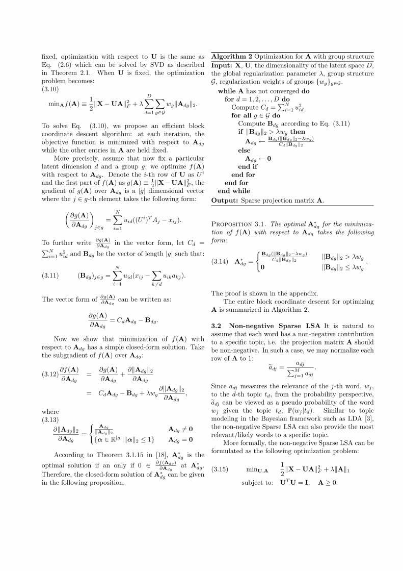
fixed, optimization with respect to U is the same asEq. (2.6) which can be solved by SVD as describedin Theorem 2.1. When U is fixed, the optimizationproblem becomes:(3.10)

minAf(A) ≡ 12‖X−UA‖2F + λ

D∑

d=1

∑

g∈Gwg‖Adg‖2.

To solve Eq. (3.10), we propose an efficient blockcoordinate descent algorithm: at each iteration, theobjective function is minimized with respect to Adg

while the other entries in A are held fixed.More precisely, assume that now fix a particular

latent dimension d and a group g; we optimize f(A)with respect to Adg. Denote the i-th row of U as U i

and the first part of f(A) as g(A) ≡ 12‖X−UA‖2F , the

gradient of g(A) over Adg is a |g| dimensional vectorwhere the j ∈ g-th element takes the following form:

(∂g(A)∂Adg

)

j∈g=

N∑

i=1

uid((U i)TAj − xij).

To further write ∂g(A)∂Adg

in the vector form, let Cd =∑Ni=1 u

2id and Bdg be the vector of length |g| such that:

(3.11) (Bdg)j∈g =N∑

i=1

uid(xij −∑

k 6=duikakj).

The vector form of ∂g(A)∂Adg

can be written as:

∂g(A)∂Adg

= CdAdg −Bdg.

Now we show that minimization of f(A) withrespect to Adg has a simple closed-form solution. Takethe subgradient of f(A) over Adg:

∂f(A)∂Adg

=∂g(A)∂Adg

+∂‖Adg‖2∂Adg

(3.12)

= CdAdg −Bdg + λwg∂‖Adg‖2∂Adg

,

where(3.13)

∂‖Adg‖2∂Adg

=

{Adg

‖Adg‖2 Adg 6= 0

{α ∈ R|g||‖α‖2 ≤ 1} Adg = 0

According to Theorem 3.1.15 in [18], A∗dg is the

optimal solution if an only if 0 ∈ ∂f(Adg)∂Adg

at A∗dg.Therefore, the closed-form solution of A∗dg can be givenin the following proposition.

Algorithm 2 Optimization for A with group structureInput: X, U, the dimensionality of the latent space D,the global regularization parameter λ, group structureG, regularization weights of groups {wg}g∈G .

while A has not converged dofor d = 1, 2, . . . , D do

Compute Cd =∑Ni=1 u

2id

for all g ∈ G doCompute Bdg according to Eq. (3.11)if ‖Bdg‖2 > λwg then

Adg ← Bdg(‖Bdg‖2−λwg)Cd‖Bdg‖2

elseAdg ← 0

end ifend for

end forend while

Output: Sparse projection matrix A.

Proposition 3.1. The optimal A∗dg for the minimiza-tion of f(A) with respect to Adg takes the followingform:

(3.14) A∗dg =

{Bdg(‖Bdg‖2−λwg)

Cd‖Bdg‖2 ‖Bdg‖2 > λwg

0 ‖Bdg‖2 ≤ λwg.

The proof is shown in the appendix.The entire block coordinate descent for optimizing

A is summarized in Algorithm 2.

3.2 Non-negative Sparse LSA It is natural toassume that each word has a non-negative contributionto a specific topic, i.e. the projection matrix A shouldbe non-negative. In such a case, we may normalize eachrow of A to 1:

adj =adj∑Mj=1 adj

.

Since adj measures the relevance of the j-th word, wj ,to the d-th topic td, from the probability perspective,adj can be viewed as a pseudo probability of the wordwj given the topic td, P(wj |td). Similar to topicmodeling in the Bayesian framework such as LDA [3],the non-negative Sparse LSA can also provide the mostrelevant/likely words to a specific topic.

More formally, the non-negative Sparse LSA can beformulated as the following optimization problem:

minU,A12‖X−UA‖2F + λ‖A‖1(3.15)

subject to: UTU = I, A ≥ 0.

According to the non-negativity constraint of A, |adj | =adj and Eq. (3.15) is equivalent to:

minU,A12‖X−UA‖2F + λ

D∑

d=1

J∑

j=1

adj(3.16)

subject to: UTU = I, A ≥ 0.

We still apply the alternating approach to solve Eq.(3.16). When A is fixed, the optimization with respectto U is the same as that in Eq. (2.6). When U isfixed, following in the same strategy as in Section 2.3,the optimization over A can be decomposed in to Mindependent subproblems, each one corresponds to acolumn of A:

(3.17) minAj≥0

f(Aj) =12‖Xj −UAj‖+ λ

D∑

d=1

adj .

We still apply the coordinate descent method tominimize f(Aj): we fix a dimension of the latent spaced; optimize f(Aj) with respect to adj while keep otherentries in f(Aj) fixed and iterate over d. More precisely,for a fixed d, the gradient of f(Aj) with respect to adj :

(3.18)∂f(Aj)∂adj

= cdadj − bd + λ,

where cd =∑Ni=1 u

2id,

bd =N∑

i=1

uid(xij −∑

k 6=duikakj).

It is easy to verify that when bd > λ, setting adj = bd−λcd

will make ∂f(Aj)∂adj

= 0. On the other hand, if bd ≤ λ,∂f(Aj)∂adj

≥ 0 for all adj ≥ 0, which further implies thatf(Aj) is a monotonic increasing function with adj andthe minimal is achieved when adj = 0. We summarizethe optimal solution a∗dj in the following proposition.

Proposition 3.2. The optimal a∗dj for the minimiza-tion f(Aj) with respect to adj takes the following form:

(3.19) a∗dj =

{bd−λcd

bd > λ

0 bd ≤ λ.

4 Related Work

There exist numerous related works in a larger contextof the matrix factorization. Here, we briefly reviewthose work mostly related to us and point out thedifference from our model.

4.1 PCA Principal component analysis (PCA) [9],which is closely related to LSA, has been widely appliedfor the dimension reduction purpose. In the contentof information retrieval, PCA first center each docu-ment by subtracting the sample mean. The resultingdocument-term matrix is denoted as Y. PCA com-putes the covariance matrix Σ = 1

NYTY and per-forms SVD on Σ keeping only the first D eigenvalues:Σ ≈ P∆D×DPT . For each centered document y, itsprojected image is PTy. In recent years, many variantsof PCA, including kernel PCA [21], sparse PCA [26],non-negative sparse PCA [25], robust PCA [14], havebeen developed and successfully applied in many areas.

However, it is worthy to point out that the PCAbased dimension reduction techniques are not suitablefor the large text corpus due to the following tworeasons:

1. When using English words as features, the textcorpus represented as X is a highly sparse matrixwhere each rows only has a small amount of nonzeroentries corresponding to the words appeared in thedocument. However, by subtracting the samplemean, the centered documents will become a densematrix which may not fit into memory since thenumber of documents and words are both verylarge.

2. PCA and its variants, e.g. sparse PCA, rely on thefact that YTY can be fit into memory and SVD canbe performed on it. However, for large vocabularysize M , it is very expensive to store M by Mmatrix and computationally costly to perform SVDon YTY.

In contrast with PCA and its variants (e.g. sparsePCA), our method directly works on the original sparsematrix without any standardization or utilizing thecovariance matrix, hence is more suitable for the textlearning task.

4.2 Sparse Coding Sparse coding, as another un-supervised learning algorithm, learns basis functionswhich capture higher-level features in the data and hasbeen successfully applied to image processing [19] andspeech recognition [8]. Although the original form ofsparse coding is formulated based on the term-documentmatrix, for the easy of comparison, in our notations,sparse coding [16] can be modeled as:

minU,A12‖X−UA‖2F + λ‖U‖1(4.20)

subject to: ‖Aj‖22 ≤ c, j = 1, . . .M,

where c is a predefined constant, A is called dictionaryin sparse coding context; and U are the coefficients.

Instead of projecting the data via A as our method,sparse coding directly use U as the projected image ofX. Given a new data q, its projected image in the latentspace can be computed by solving the following lassotype of problem:

(4.21) minbq

12‖q −AT q‖+ λ‖q‖1.

In the text learning, one drawback is that since thedictionary A is dense, it is hard to characterize thetopic-word relationships from A. Another drawback isthat for each new document, the projection operationin Eq. (4.21) is computationally very expensive.

4.3 LDA Based on the LSA, probabilistic LSA [10]was proposed to provide the probabilistic modeling, andfurther Latent Dirichlet Allocation (LDA) [3] provides aBayesian treatment of the generative process. One greatadvantage of LDA is that it can provide the distributionof words given a topic and hence rank the words fora topic. The non-negative Sparse LSA proposed inSection 3.2 can also provide the most relevant words toa topic and can be roughly viewed as a discriminativeversion of LDA. However, when the number of latenttopics D is very large, LDA performs poorly and theposterior distribution is almost the same as prior. Onthe other hand, when using smaller D, the documentsin the latent topic space generated by LDA are notdiscriminative for the classification or categorizationtask. In contrast, as we show in experiments, ourmethod greatly outperforms LDA in the classificationtask while providing reasonable ranking of the wordsfor a given topic.

4.4 Matrix Factorization Our basic model is alsoclosely related to matrix factorization which finds thelow-rank factor matrices U, A for the given matrix Xsuch that the approximation error ‖X−UA‖2F is mini-mized. Important extensions of matrix factorization in-clude non-negative matrix factorization [15], which en-forces the non-negativity constraint to X, U and A;probabilistic matrix factorization [20], which handlesthe missing values of X and becomes one of the most ef-fective algorithms in collaborative filtering; sparse non-negative matrix factorization [11, 13], which enforcessparseness constraint on either U or A; and orthogo-nal non-negative matrix factorization [6], which enforcesthe non-negativity and orthogonality constraints simul-taneously on U and/or A and studies its relationshipto clustering.

As compared to sparse non-negative matrix factor-ization [11, 13], we add orthogonality constraint to theU matrix, i.e. UTU = I, which enforces the soft clus-

tering effect of the documents. More specifically, eachdimension of the latent space (columns of U) can beviewed as a cluster and the value that a document hason that dimension as its fractional membership in thecluster. The orthogonality constraint tries to clusterthe documents into different latent topics. As comparedto orthogonal non-negative matrix factorization [6], in-stead of enforcing both non-negativity and orthogonal-ity constraints, we only enforce orthogonality constrainton U, which further leads to a closed-form solution foroptimizing U as shown in Theorem 2.1. In summary,based on the basic matrix factorization, we combine theorthogonality and sparseness constraints into a unifiedframework and use it for the purpose of semantic analy-sis. Another difference between Sparse LSA and matrixfactorization is that, instead of treating A as factor ma-trix, we use A as the projection matrix.

5 Experimental Results

In this section, we conduct several experiments on realworld datasets to test the effectiveness of Sparse LSAand its extensions.

5.1 Text Classification Performance In this sub-section, we consider the text classification performanceafter we project the text data into the latent space. Weuse two widely adopted text classification corpora, 20Newsgroups (20NG) dataset 2 and RCV1 [17]. For the20NG, we classify the postings from two newsgroupsalt.atheism and talk.religion.misc using the tf-idf of thevocabulary as features. For RCV1, we remove the wordsappearing fewer than 10 times and standard stopwords;pre-process the data according to [2] 3; and convert itinto a 53 classes classification task. More statistics ofthe data are shown in Table 1.

We evaluate different dimension reduction tech-niques based on the classification performance of linearSVM classifier. Specifically, we consider

1. Traditional LSA;2. Sparse Coding with the code from [16] and the reg-

ularization parameter is chosen by cross-validationon train set;

3. LDA with the code from [3];4. Sparse LSA;5. Non-negative Sparse LSA (NN Sparse LSA).

After projecting the documents to the latent space,we randomly split the documents into training/testing

2See http://people.csail.mit.edu/jrennie/20Newsgroups/3See http://www.csie.ntu.edu.tw/∼cjlin/libsvmtools/

datasets/multiclass.html#rcv1.multiclass

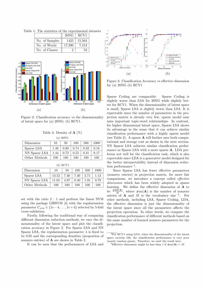
Table 1: The statistics of the experimental datasets20NG RCV1

No. of Samples 1425 15,564No. of Words 17,390 7,413No. of Classes 2 53

10 50 100 500 1000

0.6

0.65

0.7

0.75

0.8

0.85

0.9

0.95

1

1.05

1.1

Dimension of latent space

Cla

ssific

ation A

ccura

cy

Sparse LSA+SVMNN Sparse LSA+SVMLSA+SVMSparse Coding+SVMLDA+SVM

10 50 100 500 10000.4

0.5

0.6

0.7

0.8

0.9

1

Dimension of latent space

Cla

ssific

ation A

ccura

cy

Sparse LSA+SVMNN Sparse LSA+SVMLSA+SVMSparse Coding+SVMLDA+SVM

(a) (b)

Figure 2: Classification accuracy vs the dimensionalityof latent space for (a) 20NG; (b) RCV1.

Table 2: Density of A (%)(a) 20NG

Dimension 10 50 100 500 1000

Sparse LSA 1.48 0.80 0.74 0.32 0.18NN Sparse LSA 1.44 0.72 0.55 0.31 0.17Other Methods 100 100 100 100 100

(b) RCV1

Dimension 10 50 100 500 1000

Sparse LSA 13.52 7.46 7.40 2.71 1.13NN Sparse LSA 11.65 4.97 0.40 1.91 0.79Other Methods 100 100 100 100 100

set with the ratio 2 : 1 and perform the linear SVMusing the package LIBSVM [4] with the regularizationparameter Csvm ∈ {1e−4, . . . , 1e+4} selected by 5-foldcross-validation.

Firstly, following the traditional way of comparingdifferent dimension reduction methods, we vary the di-mensionality of the latent space and plot the classifi-cation accuracy in Figure 2. For Sparse LSA and NNSparse LSA, the regularization parameter λ is fixed tobe 0.05 and the corresponding densities (proportion ofnonzero entries) of A are shown in Table 2.

It can be seen that the performances of LSA and

10−2

10−1

100

101

102

103

0.5

0.55

0.6

0.65

0.7

0.75

0.8

0.85

0.9

0.95

1

Effective Dimension

Cla

ssifi

catio

n A

ccu

racy

Sparse LSA+SVMNN Sparse LSA+SVMLSA+SVMSparse Coding+SVMLDA+SVM

10−1

100

101

102

103

0.2

0.3

0.4

0.5

0.6

0.7

0.8

0.9

1

Effective Dimension

Cla

ssific

atio

n A

ccu

racy

Sparse LSA+SVMNN Sparse LSA+SVMLSA+SVMSparse Coding+SVMLDA+SVM

(a) (b)

Figure 3: Classification Accuracy vs effective dimensionfor (a) 20NG (b) RCV1

Sparse Coding are comparable. Sparse Coding isslightly worse than LSA for 20NG while slightly bet-ter for RCV1. When the dimensionality of latent spaceis small, Sparse LSA is slightly worse than LSA. It isexpectable since the number of parameters in the pro-jection matrix is already very few, sparse model maymiss important topic-word relationships. In contrast,for higher dimensional latent space, Sparse LSA showsits advantage in the sense that it can achieve similarclassification performance with a highly sparse model(see Table 2). A sparse A will further save both compu-tational and storage cost as shown in the next section.NN Sparse LSA achieves similar classification perfor-mance as Sparse LSA with a more sparse A. LDA per-forms not well for the classification task, which is alsoexpectable since LDA is a generative model designed forthe better interpretability instead of dimension reduc-tion performance 4.

Since Sparse LSA has fewer effective parameters(nonzero entries) in projection matrix, for more faircomparisons, we introduce a concept called effectivedimension which has been widely adopted in sparselearning. We define the effective dimension of A tobe #nz(A)

M , where #nz(A) is the number of nonzeroentries of A and M is the vocabulary size 5. Forother methods, including LSA, Sparse Coding, LDA,the effective dimension is just the dimensionality ofthe latent space since all the parameters affects theprojection operation. In other words, we compare theclassification performance of different methods based onthe same number of learned nonzero parameters for theprojection.

4For RCV1 using LDA, when the dimensionality of the latentspace exceeds 100, the classification performance is very poor(nearly random guess). Therefore, we omit the result here.

5Effective dimension might be less than 1 if #nz(A) < M .

Table 3: Computational Efficiency and Storage(a) 20NG

Proj. Time (ms) Storage (MB)

Sparse LSA 0.25 (4.05E-2) 0.6314

NN Sparse LSA 0.22 (2.78E-2) 0.6041

LSA 31.6 (1.10) 132.68

Sparse Coding 1711.1 (323.9) 132.68

Density of Proj. Doc. (%) Acc. (%)

Sparse LSA 35.81 (15.39) 93.01 (1.17)

NN Sparse LSA 35.44 (15.17) 93.00 (1.14)

LSA 100 (0) 93.89 (0.58)

Sparse Coding 86.94 (3.63) 90.54 (1.55)

(b) RCV1

Proj. Time (ms) Storage (MB)

Sparse LSA 0.59 (7.36E-2) 1.3374

NN Sparse LSA 0.46 (6.66E-2) 0.9537

LSA 13.2 (0.78) 113.17

Sparse Coding 370.5 (23.3) 113.17

Density of Proj. Doc. (%) Acc. (%)

Sparse LSA 55.38 (11.77) 88.88 (0.43)

NN Sparse LSA 46.47 (11.90) 88.97 (0.49)

LSA 100 (0) 89.38 (0.58)

Sparse Coding 83.88 (2.11) 88.79 (1.55)

The result is shown in Figure 3. For Sparse LSAand NN Sparse LSA, we fix the number of latent topicsto be D = 1000 and vary the value of regularizationparameter λ from large number (0.5) to small one (0)to achieve different #nz(A), i.e. different effectivedimensions. As we can see, Sparse LSA and NN SparseLSA greatly outperform other methods in the sense thatthey achieve good classification accuracy even for highlysparse models. In practice, we should try to find a λwhich could lead to a sparser model while still achievingreasonably good dimension reduction performance.

In summary, Sparse LSA and NN Sparse LSAshow their advantages when the dimensionality of latentspace is large. They can achieve good classificationperformance with only a small amount of nonzeroparameters in the projection matrix.

5.2 Efficiency and Storage In this section, we fixthe number of the latent topics to be 1000, regulariza-tion parameter λ = 0.05 and report the projection time,storage and the density of the projected documents for

different methods in Table 36. The Proj. time is com-puted as the CPU time for the projection operation andthe density of projected documents is the proportionof nonzero entries of q = Aq for a document q. Bothquantities are computed for 1000 randomly selected doc-uments in the corpus. Storage is the memory for storingthe A matrix.

For Sparse LSA and NN Sparse LSA, although theclassification accuracy is slightly worse (below 1%), theprojection time and memory usage are smaller by ordersof magnitude than LSA and Sparse Coding. In practice,if we may need to project millions of documents, e.g.web-scale data, into the latent space in a timely fashion(online setting), Sparse LSA and NN Sparse LSA willgreatly cut computational cost. Moreover, given a newdocument q, using Sparse LSA or NN Sparse LSA, theprojected document will also be a sparse vector.

5.3 Topic-word Relationship In this section, wequalitatively show that the topic-word relationshiplearned by NN Sparse LSA as compared to LDA. Weuse the benchmark data: NIPS proceeding papers7 from1988 through 1999 of 1714 articles, with a vocabulary13,649 words. We vary the λ for NN Sparse LSA so thateach topic has at least ten words. The top ten wordsfor the top 7 topics 8 are listed in Table 4.

It is very clear that NN Sparse LSA capturesdifferent hot topics in machine learning community in1990s, including neural network, reinforcement learning,mixture model, theory, signal processing and computervision. For the ease of comparison, we also list the top 7topics for LDA as in Table 5. Although LDA also givesthe representative words, the topics learned by LDA arenot very discriminative in the sense that all the topicsseems to be closely related to neural network.

5.4 Gene Function Identification with GeneGroups Information For text retrieval task, it isnot obvious to identify the separated group structuresamong words. Instead, one important application forthe group structured Sparse LSA is in gene-set identifi-cations associated to hidden functional structures insidecells. Genes could be naturally separated into groups ac-cording to their functions or locations, known as path-ways. We use a benchmark breast cancer dataset from[12], which includes a set of cancer tumor examples andeach example is represented by a vector of real values,

6“Proj.”, “Doc”, “ACC.” are abbreviations for “projec-tion/projected”, “document” and “classification accuracy”, re-spectively.

7Available at http://cs.nyu.edu/∼roweis/data/8We use D = 10. However, due to the space limit, we report

the top 7 topics.

Table 4: Topic-word learned by NN Sparse LSA

Topic 1 Topic 2 Topic 3 Topic 4

network learning network modelneural reinforcement learning datanetworks algorithm data modelssystem function neural parametersneurons rule training mixtureneuron control set likelihoodinput learn function distributionoutput weight model gaussiantime action input emsystems policy networks variablesTopic 5 Topic 6 Topic 7

function input imagefunctions output imagesapproximation inputs recognitionlinear chip visualbasis analog objectthreshold circuit systemtheorem signal featureloss current figuretime action inputsystems policy networks

e.g. the quantities of different genes found in the dataexample. Essentially, group structured Sparse LSA an-alyzes relationships between the cancer examples andgenes they contain by discovering a set of “hidden genefunctions” (i.e. topics in text case) related to the cancerand the gene groups. And it is of great interest for biol-ogists to determine which sets of gene groups, instead ofindividual genes, associate to the same latent functionsrelevant to a certain disease.

Specifically, the benchmark cancer data consistsof gene expression values from 8141 genes in 295breast cancer examples (78 metastatic and 217 non-metastatic). Based each gene’s associated “biologicalprocess” class in the standard “gene ontology” database[22], we split these 8141 genes into 1689 non-overlappedgroups, which we use as group structures in applyinggroup structured Sparse LSA.

We set the parameter λ = 1.2 and select the firstthree projected “functional” components which are rele-vant to 45 gene groups totally. The selected gene groupsmake a lot of sense with respect to their association withthe breast cancer disease. For instance, 12 gene groupsare relevant to the second hidden “function”. One se-

Table 5: Topic-word learned by LDA

Topic 1 Topic 2 Topic 3 Topic 4learning figure algorithm singledata model method generalmodel output networks setstraining neurons process timeinformation vector learning maximumnumber networks input paperalgorithm state based ratesperformance layer function featureslinear system error estimatedinput order parameter neuralTopic 5 Topic 6 Topic 7

rate algorithms functionunit set neuraldata problem hiddentime weight networksestimation temporal recognitionnode prior outputset obtain visualinput parameter noiseneural neural parametersproperties simulated references

lected group covering 10 gene variables involves in theso called “cell cycle M phase”. The cell cycle is a vitalprocess by which a single-celled fertilized egg developsinto a mature organism, or by which hair, skin, bloodcells, and some internal organs are renewed. Cancer isa disease where regulation of the cell cycle goes wrongand normal cell growth and behavior is lost. Whenthe cells multiply uncontrollably, there forms a tumor.Thus, the association of this important process to can-cer seems very reasonable. Other chosen groups involvefunctional enrichments of “cytoskeleton organization”,“regulation of programmed cell death” or “microtubule-based process”, etc. Clearly this hidden function (the2nd projection) space involves the critical “cell cycle”components relevant to important regulatory changesleading to characteristic cell grow and death. With sim-ilar analyses, we found that the first projection maps tothe space of “immune system” processes (e.g. responseto hormone stimulus ) and the third hidden function fac-tor involves in the “extracellular matrix space” amongwhich gene products are not uniformly attached to thecell surface.

Alternatively, we also perform the dimension reduc-

tion on this cancer data using the basic Sparse LSAwithout considering the group structures among genes.The resulting functional components could not be ana-lyzed as clear and as easy as the group structured SparseLSA case. The reason of the difficulty is that the dis-covered gene functions are quite large gene groups (i.e.more than 100 genes involved). They represent rela-tively high level biological processes which are essentialfor cells in any case, but not necessarily limited to thecertain cancer disease this data set is about. It is hardto argue the relationship between such a large amountof genes to the target “breast cancer” cause.

6 Conclusion

In this paper, we introduce a new model called SparseLatent Semantic Analysis, which enforces the sparsityon the projection matrix based on LSA using the`1 regularization. Sparse LSA could provide a morecompact and precise projection by selecting only a smallnumber of relevant words for each latent topic. Wefurther propose two important extensions of SparseLSA, group structured LSA and non-negative SparseLSA. A simple yet efficient alternating algorithm isadopted to learn the sparse projection matrix for allthese models. We conduct experiments on several real-world datasets to illustrate the advantages of our modelfrom different perspectives. In the future, we plan toimprove the scalability of Sparse LSA. One possibledirection is to utilize the online learning scheme to learnweb-scale datasets.

References

[1] R. Baeza-Yates, B. Ribeiro-Neto, et al. Modern in-formation retrieval. Addison-Wesley Harlow, England,1999.

[2] R. Bekkerman and M. Scholz. Data weaving: Scalingup the state-of-the-art in data clustering. In Proceed-ings of ACM International Confernece on Informationand Knowledge Management, 2008.

[3] D. Blei, A. Ng, and M. Jordan. Latent dirichletallocation. Journal of Machine Learning Research,3:993–1022, 2003.

[4] C. Chang and C. Lin. LIBSVM: a library for supportvector machines, 2001. Software available at http:

//www.csie.ntu.edu.tw/∼cjlin/libsvm.[5] S. Deerwester, S. T. Dumais, G. W. Furnas, T. Lan-

dauer, and R. Harshman. Indexing by latent semanticanalysis. Journal of the American Society for Informa-tion Science, 41, 1990.

[6] C. Ding, T. Li, W. Peng, and H. Park. Orthogonalnonnegative matrix tri-factorizations for clustering. InACM SIGKDD, 2006.

[7] J. Friedman, T. Hastie, and R. Tibshirani. Regularized

paths for generalized linear models via coordinatedescent. Journal of Statistical Software, 33(1), 2010.

[8] S. Garimella, S. Nemala, M. Elhilali, T.Tran, andH. Hermansky. Sparse coding for speech recognition.In IEEE International Confernece on Acoustics, Speechand Signal Processing, 2010.

[9] T. Hastie, R. Tibshirani, and J. Friedman. TheElements of Statistical Learning. Springer, 2001.

[10] T. Hofmann. Probabilistic latent semantic analysis.In Proceedings of Uncertainty in Artificial Intelligence,pages 289–296, 1999.

[11] P. Hoyer. Non-negative matrix factorization withsparseness constraints. Journal of Machine LearningResearch, 5:1457–1469, 2004.

[12] L. Jacob, G. Obozinski, and J.-P. Vert. Group lassowith overlap and graph lasso. In Proceedings of Inter-national Conference on Machine Learning, 2009.

[13] H. Kim and H. Park. Sparse non-negative matrix fac-torizations via alternating non-negativity-constrainedleast squares for microarray data analysis. Bioinfor-matics, 23:1495–1502, 2007.

[14] F. D. la Torre and M. Black. Robust principal com-ponent analysis for computer vision. In InternationConference on Computer Vision, 2001.

[15] D. Lee and H. S. Seung. Algorithms for non-negativematrix factorization. In Advances in Neural Informa-tion Processing Systems (NIPS), 1999.

[16] H. Lee, A. Battle, R. Raina, and A. Ng. Efficient sparsecoding algorithms. In Advances in Neural InformationProcessing Systems (NIPS), 2007.

[17] D. Lewis, Y.Yang, T. Rose, and F. Li. Rcv1: A newbenchmark collection for text categorization. Journalof Machine Learning Research, 5:361–397, 2004.

[18] Y. Nesterov. Introductory lectures on convex optimiza-tion: a basic course. Kluwer Academic Publishers,2003.

[19] B. A. Olshausen and D. J. Field. Sparse coding withan overcomplete basis set: A strategy employed by v1?Vision Research, 37:3311–3325, 1997.

[20] R. Salakhutdinov and A. Mnih. Probabilistic matrixfactorization. In Advances in Neural InformationProcessing Systems (NIPS), volume 20, 2007.

[21] B. Scholkopf, A. J. Smola, and K.-R. Muller. Kernelprincipal component analysis. In Advances in KernelMethods—Support Vector Learning. MIT Press, 1999.

[22] The Gene Ontology Consortium. Gene ontology:tool for the unification of biology. Nature Genetics,25(1):25–9, 2000.

[23] R. Tibshirani. Regression shrinkage and selection viathe lasso. Journal of the Royal Statistical Society,Series B, 58:267–288, 1996.

[24] M. Yuan and Y. Lin. Model selection and estimationin regression with grouped variables. Journal of theRoyal Statistical Society: Series B, 68:49–67, 2006.

[25] R. Zass and A. Shashua. Nonnegative sparse pca. InAdvances in Neural Information Processing Systems(NIPS), 2007.

[26] H. Zou, T. Hastie, and R. Tibshirani. Sparse principal

component analysis. Journal of Computational andGraphical Statistics, 15, 2004.

7 Appendix

7.1 Proof of Theorem 2.1 The vector form ofoptimization problem in Eq. (2.7) is:

minU −D∑

d=1

(Ud)TVd(7.22)

subject to: (Ud)TUd = 1, d = 1, . . . , D(7.23)(Uk)TUl = 0 k 6= l(7.24)

Associate the Lagrangian multipliers θdd to the con-straints in (7.23) and θkl to the constraints (7.24). Sup-pose U∗ is the optimal solution to Eq. (7.22), accordingto the KKT condition, we have

(7.25)∂L

∂Ud|U=U∗= 0, d = 1, . . . , D,

where

L = −D∑

d=1

(Ud)TVd+D∑

d=1

θdd((Ud)TUd−1)+∑

k 6=lθkl(Uk)TUl.

And Eq. (7.25) gives

Vd =D∑

k=1

θdkU∗k , d = 1, . . . D

or simply V = U∗Θ, where Θkl = θlk. According thesymmetry that (Uk)TUl = (Ul)TUk, Θ is a symmetricmatrix. Since U∗ and V are all full column rank, Θis invertible. By the assumption that V = P∆Q withPTP = QQT = I, U∗ = VΘ−1 = P∆QΘ−1. So weonly need to obtain Θ to get the optimal U∗.

To compute Θ, plugging U∗ = P∆QΘ−1 andV = P∆Q back into the original optimization problemin Eq. (2.7), the objective now becomes:

tr((U∗)TV) = tr(Θ−1QT∆PTP∆Q)(7.26)= tr(Θ−1QT∆2Q)= tr(QΘ−1QT∆2)

Define R ≡ QΘ−1QT , Eq. (7.26) becomes:

tr((U∗)TV) = tr(R∆2) =D∑

d=1

rddδ2dd.

According to the constraint that (U∗)TU∗ = I:

I = QIQT = Q(U∗)TU∗QT(7.27)= QΘ−1QT∆PTP∆QΘ−1QT

= RT∆2R

From Eq. (7.27), for any d, we have∑Dk=1 r

2dkδ

2kk = 1

which further implies that:

(7.28) r2ddδ

2dd ≤

D∑

k=1

r2dkδ

2kk = 1.

Therefore we have rddδdd ≤ 1 and upper bound of theobjective value is:

tr((U∗)TV) =D∑

d=1

rddδ2dd ≤

D∑

d=1

δdd,

The equality holds if and only if for any d = 1, . . . , D,Eq. (7.28) holds as equality which further implies R isdiagonal and R = ∆−1.

According to the definition of R, QΘ−1 = RQ =∆−1Q and the optimal solution

U∗ = P∆QΘ−1 = P∆∆−1Q = PQ.

7.2 Proof of Proposition 3.1 According to Theo-rem 3.1.15 in [18], Adg is the optimal solution if an onlyif

(7.29) 0 ∈ ∂f(Adg)∂Adg

= CdAdg −Bdg + λwg∂‖Adg‖2∂Adg

.

Assume Adg 6= 0, plugging ∂‖Adg‖2∂Adg

= Adg

‖Adg‖2 intoEq. (7.29), we have:

(7.30) Adg(Cd + λwg1

‖Adg‖2 ) = Bdg

Taking the vector `2-norm on both side of Eq. (7.30):

(7.31) ‖Adg‖2 =‖Bdg‖2 − λwg

Cd.

Since Adg 6= 0, ‖Adg‖2 should be a positive real value,which requires that ‖Bdg‖2 > λwg. Plugging Eq. (7.31)back into Eq. (7.30), we obtain that if the condition‖Bdg‖2 > λwg holds:

Adg =Bdg(‖Bdg‖2 − λwg)

Cd‖Bdg‖2 .

On the other hand, if ‖Bdg‖2 ≤ λwg, plugging Adg = 0into Eq. (7.29), we obtain that ∂‖Adg‖2

∂Adg= Bdg

λwg. It is

easy to verify that Bdgλwg

is a valid subgraident of ‖Adg‖2when Adg = 0 since ‖Bdg‖2 ≤ λwg.