Spaceborne Power Systems Preference Analyses - NASA · JPL Publication 85-5 Spaceborne Power Systems Preference Analyses Volume II: Decision Analysis J.H. Smith A. Feinberg R.F. Miles,

JPL Publication 85-5

Spaceborne Power Systems Preference Analyses Volume II: Decision Analysis ,

J.H. Smith A. Feinberg R.F. Miles, Jr.

January 15, 1985

Prepared for Defense Advanced Research Projects Agency Through an Agreement with National Aeronautics and Space Administration

by Jet Propulsion Laboratory Califomia Institute of Technology Pasadena, California

https://ntrs.nasa.gov/search.jsp?R=19850016207 2018-11-08T14:22:43+00:00Z

JPL Publication 85-5

Spaceborne Power Systems Preference Analyses Volume II: Decision Analysis

J.H. Smith A. Feinberg R.F. Miles, Jr.

January 15, 1985

Prepared for Defense Advanced Research Projects Agency Through an Agreement with National Aeronautics and Space Administration

Jet Propulsion Laboratory California Institute of Technology Pasadena, California

by

0352034

The research described in this publication was carried out by the Jet Propulsion Laboratory, California Institute of Technology and was sponsored by the Defense Advanced Research-Project Agency through an agreement with the National Aeronautics and Space Administration (NASA Task RE-182, Amendment 268; DARPA Order No. 9043).

Reference to any specific commercial product, process, or service by trade name or manufacturer does not necessarily constitute an endorsement by the United States Government, the sponsor, or the Jet Propulsion Laboratory, California Institute of Technology.

ABSTRACT

Sixteen alternative spaceborne nuclear power system concepts were ranked using multiattribute decision analysis. identify promising concepts for further technology development and the issues associated with such development.

The purpose of the ranking was to

Eleven individuals representing four groups were successfully interviewed to obtain their preferences. The four groups were: safety, systems definition and design, technology assessment, and mission analysis.

The ranking results were consistent from group to group and for different utility function models for individuals. The highest ranked systems were the heat-pipe thermoelectric systems, heat-pipe Stirling, in-core thermionic, and liquid-metal thermoelectric systems. The next group contained the liquid-metal Stirling, heat-pipe AMTEC (Alkali Metal Thermoelectric Converter), heat-pipe Brayton, liquid-metal out-of-core thermionic, and heat-pipe Rankine systems. The least preferred systems were the liquid-metal AMTEC, heat-pipe thermophotovoltaic, liquid-metal Brayton and Rankine, and gas-cooled Brayton. Although the R6D community subsequently discounted the heat-pipe reactor systems, the three non-heat-pipe technologies selected matched the top three non-heat-pipe systems ranked by this study (liquidmetal thermoelectric, in-core thermionic, and liquid-metal Stirling).

The multiattribute decision analysis process was viewed as a useful exercise for identifying options which needed further development. The analysis highlighted the need for additional and higher quality technical data as well as a need to provide an on-line capability to display source calculations interactively. An approach was suggested for displaying such traceability.

iii

FOREWORD

The Defense Advanced Projects Research Agency, together with the U.S. Department of Energy and NASA, established the Space Power-100 Devel- opment Project to assess the potential and demonstrate the feasibility of developing a nuclear power system for operation in space. The SP-100 R&D Project Office was given the responsibility to assess the state of the required technologies and make recommendations for research in support of such a development from a systems perspective. Therefore, the objectives of the assessment were to characterize and give priority to the various subsystem technologies and system concepts through the use of simulation, based on projections of the subsystem capabilities.

This report describes the multiattribute decision analysis that ranked 16 power system concepts using the preferences of 11 individuals, all knowledgeable in advanced nuclear reactor and power-conversion technologies. The advanced system concepts were designed to meet a 100-kW power requirement, 3000-kg mass requirement, and 7-year lifetime.

The report is divided into two volumes. Volume I is a summary of the multiattribute decision analysis. Volume I1 describes the multiattribute decision analysis and provides detailed technical information on the methodology and system concepts.

iv

ACKNOWLEDGMENTS

This work could not have been completed without the support of many individuals who gave generously of their time. Laboratory, the authors wish to thank Vince Truscello, Jim French, Jack Mondt, and Tosh Fujita. interviewed as to their preferences for the attributes of the systems that were evaluated.

At the Jet Propulsion

Considerable thanks are due to those individuals who were

Those organizations whose representatives participated are:

Organization Locat ion

Air Force Weapons Laboratory Jet Propulsion Laboratory Los Alamos National Laboratories NASA Lewis Research Center

Albuquerque, New Mexico Pasadena, California Albuquerque, New Mexico Cleveland, Ohio

A very special thanks is owed t o Fran Mulvehill who patiently and cheerfully typed this manuscript with its many difficult tables. Notwithstanding the help of these individuals above, the responsibility for this report rests with the authors.

This work was conducted by the Jet Propulsion Laboratory's SP-100 Project, which is a tri-agency agreement under the Defense Advanced Projects Research Agency, U.S. Department of Energy, and NASA.

V

I .

I1 .

CONTENTS

INTRODUCTION . . . . . . . . . . . . . . . . . . . . . . . . . . 1-1

A . INTRODUCTION . . . . . . . . . . . . . . . . . . . . . . . . 1-1

B . INTERVIEWS . . . . . . . . . . . . . . . . . . . . . . . . . 1-1

C . RANKINGS . . . . . . . . . . . . . . . . . . . . . . . . . . 1-3

1) . CONCORDANCE AMONG KANKINGS . . . 0 1-4

E . REPOKT . . . . . . . . . . . . . . . . . . . . . . . . . . . 1-4

METHODOLOGY . . . . . . . . . . . . . . . . . . . . . . . . . . . 2-1

A . MULTIATTRIBUTE D E C I S I O N ANALYSIS . . . . . . . . . . . . . . 2-1

B . R I S K ANALYSIS . . . . . . . . . . . . . . . . . . . . . . . 2-13

C . CONCORDANCE . . . . . . . . . . . . . . . . . . . . . . . . 2-14

I11 . OBJECTIVES. CRITERIA. AND ATTRIBUTES . . . . . . . . . . . . . . 3-1

A . INTRODUCTION . . . . . . . . . . . . . . . . . . . . . . . . 3-1

B . HIERARCHY OF OBJECTIVES. CRITERIA. AND ATTRIBUTES . . . . . 3-1

C . OBJECTIVES FOR ASSESSING SYSTEM CONCEPT ALTERNATIVES . . . . 3-2

D . OBJECTIVES. CRITERIA. AND ATTRIBUTE S E T S . . . . . . . . . . 3-4

E . DISCUSSION OF ATTRIBUTES . 3-5

F . DETERMINATION OF ATTRIBUTE SCALES . . . . . . . . . . . . . 3-7

I V . ALTERNATIVES AND STATE DATA . . . 4-1

A . INTRODUCTION . . . . . . . . . . . . . . . . . . . . . . . . 4-1

B . ALTERNATIVE SYSTEM CONCEPTS . . . . . . . . . . . . . . . . 4-1

C . SYSTEM CONCEPT ATTRIBUTE STATE DATA . . . . . . . . . . . . 4-2

vii

V . INTERVIEWS . . . . . . . . . . . . . . . . . . . . . . . . . . . 5-1

A INTRODUCTION . . . . . . 5-1

Be INTERVIEWEES . . . 5-1

C . INTERVIEW PROCESS . . . . . . . 5-2

De SAMPLE QUESTIONS . . . 5-4

E . INTERVIEW PROCESS REFERENCES . . . . . . . . . . . . . . . . 5-4

F . INTERVIEW RESULTS . . . . . . . . . . . . . . . . . . . . . 5-4

V I . RANKING ANALYSIS AND DISCUSSION . . . . . . . . . . . . . . . . . 6-1

A . OVERVIEW O F THE: DECISION ANALYSIS RESULTS . . . . . . . . . 6-1

B . MATEUS COMPUTER RUNS . . . . . . . . . . . . . . . . . . . . 6-1

C . MULTIATTRIBUTE RESULTS FOR NOMINAL ATTRIBUTE DATA . . . . . 6-3

D . RESULTS O F VARIATIONS ON MULTIATTRIBUTE NOMINAL DATA . . . . 6-3

E . GENERAL CONCLUSIONS . . . . . . . . . . . . . . . . . . . . 6-12

F . CRITIQUE OF MULTIATTRIBUTE D E C I S I O N ANALYSIS METHODOLOGY . . . . . . . . . . . . . . . . . . . . . . . . 6-12

V I 1 . CONCORDANCE O F RANKINGS . . . . . . . . . . . . . . . . . . . . . 7-1

A . INTRODUCTION . . . . . . . . . . . . . . . . . . . . . . . . 7-1

V I 1 1 . REFERENCES . . . . . . . . . . . . . . . . . . . . . . . . . . . 8-1

Figures

1.1 . R a n k i n g Methodology F l o w D i a g r a m . . . . . . . . . . . . . . 1-2

2.1 . R e l a t i o n s h i p b e t w e e n S y s t e m V a l u e Models . . . . . . . . . . 2-3

2.2 . T y p i c a l D e c i s i o n Tree . . . . . . . . . . . . . . . . . . . 2-5

2.3 H i e r a r c h y of O b j e c t i v e s . C r i t e r i a . and A t t r i b u t e s . 2-7

2.4 . E x a m p l e s of Increasing U t i l i t y Funct ions f o r D i f f e r e n t R i s k A t t i t u d e s . . . . . . . . . . . . . . . . . . 2-15

v i i i

3.1 . Hierarchy of Objectives. Subobjectives. Criteria. and Attributes for Spaceborne Power System Concepts . . . . . . 3-6

5.1 . Decision-Analysis Interview Flow Chart . . . . . . . . . . 5-3 5.2 . Sample Interview Question. Radiator Area . . . . . . . . . 5-5 5.3 . Sample of Interview Question. Order of

Attribute Importance . . . . . . . . . . . . . . . . . . . 5-6 5.4 . Sample of Interview Question. Importance of

Radiator Area . . . . . . . . . . . . . . . . . . . . . . . 5-7

Tables

2.1 . Table of Critical Values of "S" in the Kendall Coefficient of Concordance . . . . . . . . . . . . . . . . 2-16

3.1 . Requirements for Space Power Concepts . . . . . . . . . . . 3-4 3.2 . Attributes with Ranges for Cost and Performance . . . . . . 3-8 4.1 . Alternative System Concepts with Abbreviations . . . . . . 4-1 4.2 . Attribute State Data for the Sixteen Alternative

System Concepts . . . . . . . . . . . . . . . . . . . . . . 4-3

4.3 . Attributes within Range x 10% of Most Preferred State . . . . . . . . . . . . . . . . . . . . . . 4-4

5.1 . Preference Data for All Interviews . . . . . . . . . . . . 5-8 5.2 . Preference Data For Interviews by Group

(a) Safety Area . . . . . . . . . . . . . . . . . . . . . 5-9

(b) System Definition and Design Area . . . . . . . . . . 5-10 (c> Technology Assessment Area . . . . . . . . . . . . . . 5-11

5.3 . Preference Data from Interviews. Importance of Attributes . . . . . . . . . . . . . . . . . . . . . . . . 5-12

5.4 . Ranking of Attribute Importance . . . . . . . . . . . . . . 5-13 6.1 . Rankings for All Individuals f o r Set 1 . . . . . . . . . . 6-4 6.2 . Multiattribute Decision Analysis: Summary of Advanced

Vehicle Rankings Using Nominal States. Multiplicative Model. 5-pt Utilities . . . . . . . . . . . . . . . . . . . 6-5

6.3 . Rankings by Each of the Eight Attributes . . . . . . . . . 6-6

ix

6-4(a) Multiattribute Decision Analysis: Summary of System Concept Rankings; Results for Safety Group . . . . . . . . 6-7

6-4(b) Multiattribute Decision Analysis: Summary of System Concept Rankings; Results for Systems Definition and Design Group . . . . . . . . . . . . . . . . 6-8

6-4(c) Multiattribute Decision Analysis: Summary of System Concept Rankings; Results for Technology Assessment Group . . . . . . . . . . . . . . . . . . . . . 6-9

7-1. Summary of Kendall's Coefficient of Concordance (W) and the Associated Chi-square Values (X2) for all Runs: Individuals Within Groups . . . . . . . . . . . . . . . . . 7-2

7-2. Summary of Kendall's Coefficient of Concordance (W) and the Associated Chi-square Values ( X 2 ) for all Runs: Group Decision Rules . . . . . . . . . . . . . . . . . . . 7-3

APPENDICES

A. QUESTIONNAIRE USED FOR INTERVIEWS . . . . . . . . . . . . . A-1 B. COMPUTER PROGRAMS USED . . . . . . . . . . . . . . . . . . B-1

X

SECTION I

INTRODUCTION AND SUXMARY

A. INTRODUCTION

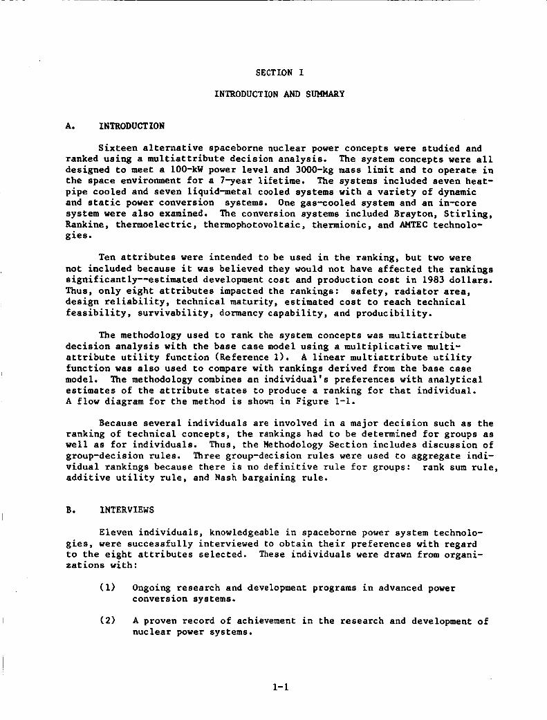
Sixteen alternative spaceborne nuclear power concepts were studied and ranked using a multiattribute decision analysis. The system concepts were all designed to meet a 100-kW power level and 3000-kg mass limit and to operate in the space environment for a 7year lifetime. The systems included seven heat- pipe cooled and seven liquid-metal cooled systems with a variety of dynamic and static power conversion One gas-cooled system and an in-core system were also examined. The conversion systems included Brayton, Stirling, Rankine, thennoelectric, thermophotovoltaic, thermionic, and AMTEC technologies.

systems.

Ten attributes were intended to be used in the ranking, but two were not included because it was believed they would not have affected the rankings significantly-estimated development cost and production cost in 1983 dollars. Thus, only eight attributes impacted the rankings: safety, radiator area, design reliability, technical maturity, estimated cost to reach technical feasibility, survivability, dormancy capability, and producibility.

The methodology used to rank the system concepts was multiattribute decision analysis with the base case model using a multiplicative multiattribute utility function (Reference 1). A linear multiattribute utility function was also used to compare with rankings derived from the base case model. The methodology combines an individual's preferences with analytical estimates of the attribute states to produce a ranking for that individual. A flow diagram for the method is shown in Figure 1-1.

Because several individuals are involved in a major decision such as the ranking of technical concepts, the rankings had to be determined for groups as well as for individuals. Thus, the Methodology Section includes discussion of group-decision rules. Three group-decision rules were used to aggregate individual rankings because there is no definitive rule for groups: additive utility rule, and Nash bargaining rule.

rank sum rule,

B. INTERVIEWS

Eleven individuals, knowledgeable in spaceborne power system technolo-

These individuals were drawn from organi- gies, were successfully interviewed to obtain their preferences with regard to the eight attributes selected. zations with:

(1) Ongoing research and development programs in advanced power conversion systems.

(2 ) A proven record of achievement in the research and development of nuclear power systems.

1- 1

SPECIFY ALTERNATIVES

ESTABLISH ATTRIBUTES

OBTAIN INDIVIDUAL PREFERENCES

PREPARE DATA FOR RANKING

RANK & ANALYZE ALTERNATIVES r- BY INDIVIDUAL

RANK & ANALYZE ALTERNATIVES

BY GROUP

DOCUMENT RESULTS

OBTAIN ATTRIBUTE STATE DATA

I

Figure 1-1. Ranking Methodology Flow Diagram

1-2

(3) An understanding of space environment issues which have direct impact on developing nuclear power technologies for space applications.

These individuals represented four distinct groups:

Safety Group. issues from ground development through launch, on-orbit operation, and re-entry.

This group was concerned with a range of safety

Systems Definition and Design Group. This group was concerned with the design issues and options involved in the development and deployment of the technology.

Technology Assessment Working Group. This group was involved in assessing the technical issues facing the demonstration of technical feasibility for such power systems.

Mission Analysis Group. possible mission users who would utilize the system concepts.

This area involved the concerns of

C. RANKINGS

Rankings were calculated for the 11 individuals successfully interviewed and for the four groups that they represented. Rankings for the individuals were calculated using several different multiattribute utility models and with each of the attributes removed. Rankings for the groups were calculated using three different group decision rules.

The ranking results were quite consistent from group to group and for different utility function models for individuals. Generally, the rankings fell into four areas: most preferred concepts (those high-ranking systems whose rankings were unchanged by various assumptions about the multiattribute decision model), preferred (those systems whose (high) rankings varied with changes in the multiattribute decision model assumptions but remained clustered together near the high end of the rankings), intermediate (those systems whose rankings varied with changes in the multiattribute decision model assumptions but remained clustered together near the low end of the rankings), and least preferred (those low-ranking systems whose rankings were virtually unchanged by various assumptions about the multiattribute decision model). The most preferred systems were the heat-pipe thermoelectrics (HTEP, HTEPa). The preferred systems were the heat-pipe Stirling (HSH), in-core thermionic (ICT) , and liquidmetal thermoelectric (LTEP) . The intermediate systems were the liquid-metal Stirling (LSH), heat-pipe AMTEC (HAP), heat-pipe Brayton (HBO), liquidrnetal out-of-core thermionic (LOCTP), and heat-pipe Rankine (HRL). The least preferred concepts were the liquid-metal AMTEC (LAP), heat-pipe thermophotovoltaic (HTPVP) , liquid-metal Brayton (LBO), liquid-metal Rankine (LRL), and gas-cooled Brayton (GBH).

The above rankings were used to initiate planning for the technical development of promising options within the project time frame. ticular, the rankings were used to identify technology areas for more

In par-

1-3

comprehensive research. nated almost a l l of t h e heat-pipe concepts as being r i s k i e r than previous ly thought w i th a l imi ted ope ra t iona l database. a n a l y s i s had a d i r e c t impact on t h e l i s t of systems which were candida tes f o r t h i s downscoping e f f o r t . t h e remaining sys t ems ( a f t e r removing t h e heat-pipe systems) was substan- t i a l l y t h e same wi th t h e pre l iminary resu l t s obta ined here in .

A subsequent technology downscoping e v a l u a t i o n e l imi -

The r e s u l t s of t h e present

It should be noted t h a t t h e rank o rde r ing of

D. CONCORDANCE AMONG RANKINGS

The concordance o r agreement among the rankings was c a l c u l a t e d f o r i nd iv idua l s within groups, d i f f e r e n t group d e c i s i o n r u l e s , and d i f f e r e n t m u l t i a t t r i b u t e u t i l i t y models. ou t t o a s c e r t a i n how robus t t h e rankings were. I n gene ra l , t h e rankings were h ighly concordant ac ross ind iv idua l s , d i f f e r e n t group d e c i s i o n r u l e s , and d i f f e r e n t m u l t i a t t r i b u t e u t i l i t y models, implying t h a t t h e rankings were indeed robus t .

The concordance c a l c u l a t i o n s were c a r r i e d

The robustness of t h e rankings w a s due t o (1 ) a gene ra l consensus regard ing t h e importance of t h e s a f e t y and t e c h n i c a l ma tu r i ty a t t r i b u t e s ; and (2) t h e dominance of t h e system d a t a i n pre-determining t h e high and low end rankings.

E. REPORT

This Volume c o n s i s t s of seven s e c t i o n s : an i n t r o d u c t i o n (Sec t ion I>; methodology (Sect ion 1 1 ) ; d e s c r i p t i o n of t h e a t t r i b u t e s (Sec t ion 111); l i s t i n g of t h e a l t e r n a t i v e s and s t a t e d a t a (Sec t ion IV); summary of t h e in te rv iews and preference d a t a (Sec t ion V); p r e s e n t a t i o n and a n a l y s i s of t h e rankings and resu l t s (Sec t ion V I ) ; and summary of t h e concordance of rankings (Sec t ion VII).

1-4

SECTION I1

METHODOLOGY

This section describes and illustrates the methodology used to evaluate and compare alternative spaceborne power concepts. of a number of steps which, in short, characterize the alternative approaches under different design options and operating environments, assign utility values to the alternatives, and rank the alternatives based on these utilities. methodologies, and attribute sets were carried out and are discussed in Section VII.

The methodology consists

Tests of concordance of the rankings for different individuals, groups,

The evaluation methodology may be summarized as follows. The process begins with the selection of a set of descriptive but quantifiable attributes designed to characterize each system. Values for this set of attributes are then generated for each alternate approach that specify its response (e.g., performance or cost) under different design options and operating environments. (The attributes are discussed in Section 111.1 A decision tree can be constructed to relate economic, technological, and environmental uncertainties (i.e., the operating environment) to the cost and performance outcomes (i.e., attribute values) of the alternative power concepts. Multiattribute utility functions that reflect the preferences and perceptions of knowledgeable individuals are generated, based on interviews with selected personnel. tions are then employed to generate a multiattribute utility value for each system, based on its characteristics under the scenarios reflected within the decision tree. utility value €or each alternative, the expected value being taken over the scenario probability distribution. Alternative systems are ranked according to this expected multiattribute utility value.

The func-

The decision tree is used to compute an expected multiattribute

A. MULTIATTRIBUTE DECISION ANALYSIS

1. Overview

Multiattribute decision analysis is a methodology for providing information to decisionmakers for comparing and selecting from among complex alternative systems in the presence of uncertainty. The methodology of multiattribute decision analysis is derived from the techniques of operations research, statistics, economics, mathematics, and psychology. Thus, research- ers from a wide range of disciplines have participated in the development of multiattribute decision analysis. The first books and papers on the subject appeared in the late 1960s (References 2 through 5 ) . The most practical, extensive, and complete presentation of an approach to multiattribute decision analysis is given in the 1976 work of Keeney and Raiffa (see Reference 1). Although several approaches to multiattribute decision analysis have been developed (References 6 through 191, the method used in this report corresponds to an abbreviated form of that of Keeney and Raiffa. A brief introduction to multiattribute decision analysis, discussing primarily the Keeney and Raiffa methodology, is given in Feinberg and Miles (Reference 20). The assumptions needed for the abbreviated form used here are discussed at the end of subsection A-4.

2-1

Every systems analysis involving the preference ranking of alternative systems, whatever the specific methodology, requires two kinds of models. is a "system model'' and is representative of the alternative systems (including any uncertainties) under consideration. The other is a "value model'' and is representative of the preference structure of the decisionmakers whose preferences are being assessed.

One

The system model describes the alternative systems available to the decision-makers in terms of the risk and possible outcomes that could result from each system. associated with each alternative system and from the uncertain environment in which the systems would be required to perform. possible consequences of the alternative systems. risk, the selection of a specific system does not in general guarantee a specific outcome, but rather results in a probabilistic situation in which only one of several outcomes may occur. attributes, then form the input to the value model. The value model assesses the outcomes in terms of the preferences of the decision-makers for the various outcomes. The measurable attributes of the outcomes are aggregated algebrai- cally in a formula (called a multiattribute utility function) whose functional form and parameters are determined by the preference structure of the decision- makers. value for each outcome (outcome utility). back into the system model where an alternative system utility can be calculated for each alternative system simply by taking the expected utility value of the outcomes associated with each alternative system. These alternative system utilities then define a preference ranking over the alternative systems, with greater alternative system utilities being more preferred.

Risk arises from the technological and economic uncertainty

The outcomes describe the Because of the element of

These outcomes, with their measurable

The output of the value model is a multiattribute utility function These outcome utilities are entered

The relationship between the system model and the value model is illustrated in Figure 2-1, which shows that the combination of a selected system and a realized state of uncertainty results in the output from the system model to the value model of a specific outcome. The output of the value model is an outcome utility. The probabilistic combination of the outcome utilities of the outcomes associated with a specific alternative system determine an alternative system utility in the system model. Comparison of the alternative system utilities for all the alternative systems under consideration results in an alternative system ranking as the output from the system model.

2. Decision Trees

Decision trees are used to represent the system model and the inputs to the system model at the gross €eve1 required for the decision analysis. sented by squares), with alternative paths emanating from them; and by chance nodes (represented by circles), with probabilistic paths emanating from them. All paths either terminate at another node or terminate at an outcome, which is a description of the consequence of traversing a specific set of paths and nodes through the decison tree from beginning to end. There can be only one originating node (either a decision node or a chance node). There can be many outcomes terminating the decision tree, depending on the complexity of the decision tree.

Decision trees are graphically depicted by decision nodes (repre-

2- 2

UNCERTAINTY

L ALTERNATIVE ALTERNATIVE SYSTEMS

OUTCOME DESCRIPTIONS

SYSTEM MODEL

VALUE MODEL

SYSTEM RANKING

I

OUTCOME UTlLlT IES

I I

Figure 2-1. Relat ionship Between System Value Models

2-3

Figure 2-2 shows a typical decision tree, terminating in 10 outcomes. The symbols "Di" stand for the ith decision node ("D" for decision). symbols "Pj" stand for the jth cGnce node (I'P'' for probabilistic). symbols "Ck'l stand for the k z outcome ("C" for consequence). emanating from a decision node corresponds to an alternative that the decisionmakers can select, where "A~R" stands for the at the ith decision node. path at each decision node. corresponds to one of the uncertain and uncontrollable chance states that can occur at that node, where p state will be realized at the jl!! chance node. The pjms must obey the laws of probability theory. from a chance node, and the pjms must sum to 1.0.

The

Every path The

alternative selected The decision-makers can select one and only one Every path Pjm emanating from a chance node

is the probability that the m g chance

Thus, o z and only one chance path can be realized

The chance nodes and their associated chance paths and probabilities are This report shall refer to called "gambles" or "lotteries" in the literature.

them as gambles. An example of a gamble would be a flip of a coin, which could be expected to come up heads 50% of the time and tails 50% of the time. Graphically, such a gamble would be displayed as:

HEADS

TAILS

Figure 2-2 has an example of every kind of node-path-outcome relationship. There are examples of decision-node to decision-node paths, decision- node to chance-node paths, decision-node to outcome paths, chance-node to decision-node paths, chance-node to chance-node paths, and chance-node to outcome paths.

As an example of how the decision tree might be traversed, imagine that the decision-maker selects Alternative Path A12 at Decision Node D1, where he must start. This leads to Chance Node PI where Chance Path Pi3 is realized, leading to Chance Node P3, where Chance Path P32 is realized, and terminates with Outcome (210.

3. Objectives Hierarchy

The outcomes that terminate the decision tree are to be described in terms of an objectives hierarchy that (1) expresses the preference structure of the decision-makers, and (2 ) is constructed in a manner compatible with the quantification and mathematical conditions required by a multiattribute utility function of the value model. The objectives hierarchy expresses the preference structure of the decisionmakers in ever increasing detail as one proceeds down through the hierarchy from overall objective to a lower-level hierarchy of subobjectives. Below the subobjectives are "criteria." The criteria must permit

2-4

w w w I I I I- I - 1 I- .. .. ..

N I

N

2-5

the quantification of performance of the alternatives with respect to the subobjectives. Associated with each criterion is an "attribute," a quantity that can be measured and for which the decision-makers can express preferences for its various states. Figure 2-3 shows an objectives hierarchy with the associated attributes.

The set of attributes must satisfy the following requirements for the value model to be a valid representative of the preference structure of the decision-makers:

Completeness: the factors to be considered in the decisionmaking process.

The set of attributes should characterize all of

Comprehensiveness: its associated criterion.

Each attribute should adequately characterize

Importance: rion in the decisionmaking process, at least in the sense' that the

Each attribute should represent a significant crite-

attribute has the potential for affecting the preference ordering of the alternatives under consideration.

Measurability: tively or subjectively quantified; technically, this requires that it be possible to establish an attribute utility function for each attribute.

Each attribute should be capable of being objec-

Familiarity: decision-makers in the sense that they should be able to identify preferences for different states of the attribute for gambles over the states of the attribute.

Each attribute should be understandable to the

Nonredundancy: Two attributes should not measure the same criterion, thus resulting in double counting.

Independence: The value model should be so structured that changes within certain limits in the state of one attribute should not affect the preference ordering for states of another attribute or the preference ordering for gambles over the states of another attribute.

Attribute Utility Functions and the Multiattribute Utility Function

The set of attributes associated with the objectives' hierarchy must satisfy the aforementioned measurability and mathematical requirements. If it satisfies these requirements, then it is possible to formulate a mathematical function (called a multiattribute utility function) that will assign numbers (called outcome utilities) to the set of attribute states characterizing an outcome. of Keeney and Raiffa (Reference 1). Keeney and Raiffa multiattribute utility function have the properties of Von Neumann and Morgenstern utilities (Reference 231, that is:

The multiattribute utility function that was used is that The outcome utilities generated by the

2-6

1-r I--€ -€ €I

1

1 1

4J

Y

rl $4 V

s 0 rw 0

2 $4 9) rl X

m I

N

2-7

(1) Greater outcome utility values correspond to more preferred ou t c ome s .

( 2 ) 'The utility value to be assigned to a gamble is the expected value of the outcome utilities of the gamble.

The mathematical axioms that must be valid for these two properties to hold were first derived by Von Neumann and Morgenstern (see Reference 2 3 ) . Elementary expositions of these axioms are given in Hadley (Reference 24) and Luce and Raiffa (Reference 25). DeGroot (Reference 26). An advanced exposition is given in Fishburn (Reference 27) .

An intermediate exposition is given in

To every outcome "C," an N-dimensional vector of attributes x = (xi, ..., XN) Most of the attribute requirements are

will be associated, the set of which satisfy the attribute requirements presented in the preceding subsection. self-evident. The seventh requirement, that of attribute independence, is a condition that makes it possible to consider preferences between states of a specific attribute, without consideration of the states of the other N-1 attributes. It is thus possible to construct an attribute utility function that is independent of the other attribute states, and which, like the outcome utility function, satisfies the Von Neumann and Morgenstern properties for utility functions. This condition of independence, or some equivalent mathematical condition (see Reference 1 for alternative formulations), is necessary for the Keeney and Raiffa methodology. is valid in practice, or more correctly, to test and identify the bounds of its validity.

It is necessary to verify that this condition

To continue the discussion from this point on, it is necessary to introduce some mathematical notation:

xn = The state of the nth - attribute.

xg = The least-preferred state to be considered for the nfi attribute.

xi = The most-preferred state to be considered for the n G attribute.

x = The vector (xi, ..., XN) of attribute states characterizing a specific outcome.

xo = An outcome constructed from the least preferred states of all 0 the attributes. xo = (xl, ..., xi).

* x = An outcome constructed from the most preferred states of all * * attributes. x* = (XI, ..., XN). -

(Xn, x:) = An outcome in which all attributes except the n e attribute are at their least-preferred state.

un(xn> = The attribute utility of the nth - attribute. u(x) = The outcome utility of the outcome x.

kn = The attribute scaling constant for the n 3 attribute. * kn = u(xn, xg).

k The master scaling constant for the multiattribute utility equation. It is an algebraic function of the kns.

With this mathematical notation, the discussion can proceed to how attribute utility functions and the attribute scaling functions are assessed. The mathematics permit the arbitrary assignments:

un<xg> = 0.0

and

* un(xn) = 1.0

Thus, the attribute utility function values will range from 0.0 to 1.0. Attribute utilitx function values for attribute states xn intermediate between x$ and xn are assessed by determining a value of pn such that the decision makers or their designated experts are indifferent between receiving xn for sure - or a gamble that yields xg with probability Pn or xn with probability 1-pn. Graphically, assess pn, so that: *

where "-" means indifference. It follows from the mathematics that:

This indifference relation is repeated for various attribute states until either a continuous utility function can be approximated or enough discrete points have been assessed for the attribute states under consideration in the analysis.

A similar approach is used t o assess the scaling constants k,. for kn is assessed such that the following indifference relationship holds:

A value

2-9

With this assessed information, the multiattribute utility equation can be solved to yield an outcome utility value for any outcome under consideration. The multiattribute utility function can now be stated:

If N

n=l kn # 1.0

then

N

n= 1 u(x) = [l + k k n n n u (x )] - 11

where the master scaling constant k is solved for from the equation:

N

n-1 l + k = ( l + k k n )

If

2 kn = 1.0 n-1

then there is an additive utility function,

N u(x> = kn un(xn)

n=l

The outcome utility function values, like the attribute utility function values, will all range from 0.0 to 1.0 with u(xo) = 0.0 and u(x*) = 1.0. Although the mathematical equations appear complex, they can be easily solved, and the information required in the interviews with the decision-makers can be minimized. An extended discussion of these equations, their solution, and the assessment of the required data, together with examples taken from actual applications, is given in Keeney and Raiffa (see Reference 1).

2-10

In this study, an abbreviated form of Keeney and Raiffa's methodology was used to reduce the interview time for the interviewee. made that utility independence of each attribute implies pair-wise utility independence (i.e., the attributes exhibit utility independence when taken two at a time). This assumption allows the use of Formulation ( 4 ) of Theorem 6.2 of Keeney and Raiffa (see Reference 1). Given single-attribute utility independence, the authors could not construct a realistic example where pair-wise utility independence would be violated.

An assumption was

The abbreviated form satisfies the multilinear model shown in Theorem 6 . 3 of Keeney and Raiffa. However, the multilinear form requires the assessment of 2n-2 scaling constants, where n is the number of attributes. With n = 8 attributes, 254 scaling constants would be needed, requiring extensive time for both the interviewer and interviewee.

5. Ranking the Alternative Systems

The steps needed prior to ranking the alternatives are: the development of a decision tree, the determination of probabilities for the decision of an objectives hierarchy, the quantification of the criteria in terms of measurable attributes, and the determination of a multiattribute utility function with attribute utility functions and attribute scaling constants corresponding to the preference structure of the decision makers. The ranking of the alternative systems proceeds as follows (see Figure 2-2):

(1) Use the multiattribute utility function to calculate outcome utilities for all of the outcomes of the decision tree.

(2) Calculate a utility value to be assigned to all chance nodes by taking the expected utility value of the utilities assigned to the termination of the chance paths of the chance nodes. The chance paths may terminate at outcomes, other chance nodes, decision nodes, or a combination of these.

(3 ) Calculate a utility value for all decision nodes by selecting the decision path that terminates in an outcome, chance node, or decision node with the highest utility value. value assigned to the decision node.

The utility value of that path shall be the utility

The decision tree for this study has an originating decision node whose decision paths correspond to the alternative systems under consideration. Steps (1) through ( 3 ) are performed by starting with the outcomes as shown in Figure 2-2 and assigning utility values to these outcomes. Then Steps (2) and ( 3 ) are performed by a "folding back" process, proceeding from right to left, and assigning utility values to the chance nodes and the decision nodes. Finally, utility values are assigned to the decision paths emanating from the orginating decision node on the left. These utility values are the ones assigned to the alternative systems. Because greater utility values correspond to more preferred systems, a rank order in preference for the alternative system can be assigned in correspondence with the utility values. able and tangible measure of the strength of preference between the alternative

A quantifi-

2-1 1

sys t ems can be obtained by r e fe renc ing each a l t e r n a t i v e system t o a se t of sys t ems where only one a t t r i b u t e , such as i n i t i a l c o s t , i s v a r i e d (References 30 and 31). The d i f f e r e n c e s i n t h e a t t r i b u t e s ta tes of t h i s one a t t r i b u t e va r i ed i n order t o o b t a i n i n d i f f e r e n c e t o each of t h e a l t e r a t i v e s y s t e m s w i l l provide a tangib le measure of t h e s t r e n g t h of preference between t h e a l t e r n a t i v e systems.

6. Group Decision Models

Throughout t h i s s e c t i o n , "decision-makers" has been c o n s i s t e n t l y d iscussed i n the p l u r a l . It i s t r u e t h a t i n American s o c i e t y , co rpora t e and government (execut ive branch) d e c i s i o n s are u l t i m a t e l y t h e r e s p o n s i b i l i t y of one person, though t h e same cannot be s a i d f o r e i t h e r t h e l e g i s l a t i v e branch of government o r t h e vo t ing publ ic . Thus, depending upon t h e con tex t , i t may be more appropr ia te t o speak of decis ion-maker i n t h e s ingu la r . Never the less , when one person holds the u l t i m a t e r e s p o n s i b i l i t y f o r t h e dec i s ion , t h i s person may e l e c t t o de lega te the decision-tnaking r e s p o n s i b i l i t y t o a group, o r a t l e a s t cons ide r t h e preferences of s e v e r a l o t h e r s p r i o r t o making t h e dec is ion .

Unfortunately, t h e r e p re sen t ly e x i s t no a n a l y t i c a l models f o r group d e c i s i o n making t h a t do not v i o l a t e some i n t u i t i v e l y d e s i r a b l e condi t ions . Arrow (Reference 30) was the f i r s t t o demonstrate t h i s f a c t . Extensive d i scuss ions of group dec i s ion making can be found i n Fishburn (Reference 311, Luce and Rai f fa ( s e e Reference 251, and Sen (Reference 32). The b e s t t h a t can be done i s t o look a t a range of group d e c i s i o n models, and where consensus o f the/models i s found, d e f i n e t h a t as t h e consensus of t h e group (References 33 and 34).

The three group d e c i s i o n r u l e s t h a t w i l l be considered i n t h i s r e p o r t are t h e Rank Sum Rule, t he Nash Bargaining Rule, and the Addit ive U t i l i t y R u l e . (The Majority Decis ion Rule, which o r i g i n a l l y w a s considered f o r use i n t h i s a n a l y s i s , was not employed because of unsolved t h e o r e t i c a l problems t h a t a r i s e when more than two a l t e r n a t i v e s are involved) .

The Rank Sum R u l e (References 30 and 35) i n t h e s l i g h t l y modified form proposed he re , r e q u i r e s t h e c a l c u l a t i o n of t h e sum of t h e o r d i n a l ranks f o r each a l t e r n a t i v e , wi th t h e a l t e r n a t i v e r ece iv ing t h e lowest rank sum being most p re fe r r ed . Young (Reference 36) has s t a t e d f o u r axioms t h a t are neces- s a r y and s u f f i c i e n t f o r any c o l l e c t i v e choice r u l e t o be equ iva len t t o t h e Borda Rule.

The Nash Bargaining Rule c a l c u l a t e s t h e product of t h e u t i l i t i e s ass igned by a l l t h e ind iv idua l s t o a n a l t e r n a t i v e . The a l t e r n a t i v e s wi th g r e a t e r u t i l i t y product are more p r e f e r r e d , and from t h i s a group p re fe rence o rde r can be es tab l i shed . The Nash Bargaining Rule s a t i s f i e s Nash's f o u r axioms of "fairness" (Reference 37). A s t h e number of decision-makers inc rease , t h e Nash u t i l i t i e s decrease because t h e i n d i v i d u a l u t i l i t i e s equa l 1.0. Hence, for even t e n decision-makers, t h e Nash u t i l i t i e s are small . Without l o s s of g e n e r a l i t y , the Nash u t i l i t i e s can be re-scaled by t ak ing t h e n t h r o o t of t h e product of t h e i n d i v i d u a l u t i l i t i e s , where n i s t h e numbeyof dec i s ionmaker s i n the group.

2-12

The modern formulation of the Additive Utility Rule is that of Harsanyi (Reference 38). assigned by the individuals to each alternative, with higher average utility values being more preferred.

The Additive Utility Rule averages the utility values

It should be re-emphasized that there is no theoretically compelling reason to use the results of any of these group decision rules, but they do provide information concerning the collective preferences of the decision- makers.

B. RISK ANALYSIS

1. Introduction

Another element of the sensitivity analysis effort is that of risk analysis. Risk is defined as the possibility of loss or injury. This subsection explains and illustrates the elements of risk analysis and describes how risk analysis is incorporated into the multiattribute decision model and into the sensitivity analysis.

2. Risk-Analysis Elements

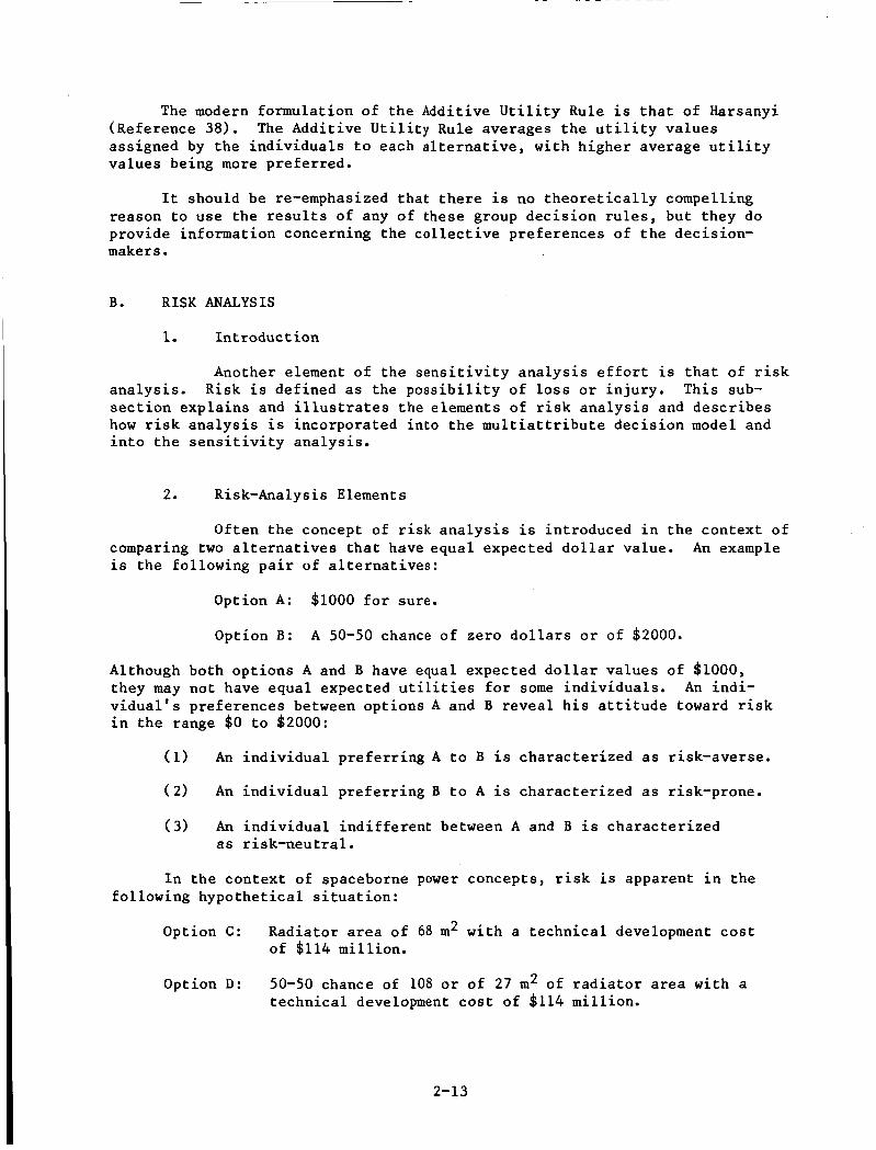
Often the concept of risk analysis is introduced in the context of comparing two alternatives that have equal expected dollar value. is the following pair of alternatives:

An example

Option A: $1000 for sure.

Option B: A 50-50 chance of zero dollars or of $2000.

Although both options A and B have equal expected dollar values of $1000, they may not have equal expected utilities for some individuals. vidual's preferences between options A and B reveal his attitude toward risk in the range $0 to $2000:

An indi-

(1) An individual preferring A to B is characterized as risk-averse.

( 2 ) An individual preferring B to A is characterized as risk-prone.

( 3 ) An individual indifferent between A and B is characterized as risk-neutral.

In the context of spaceborne power concepts, risk is apparent in the following hypothetical situation:

Option C: Radiator area of 68 m2 with a technical development cost of $114 million.

Option D: 50-50 chance of 108 or of 27 m2 of radiator area with a technical development cost of $114 million.

2-13

Although both options C and D have equal expected radiator area and equal development costs, individuals may exhibit different preferences, as with the previous dollar example. characterized as risk-averse, etc.

An individual preferring Option C to Option D is

Risk attitude implies a certain shape of the individual's utility function and vice versa (see References 1 and 3 ) . A risk-averse attitude for an attribute is equivalent to a concave utility function for that attribute. Also, risk-proneness is equivalent to a convex utility function; and finally, risk-neutrality is equivalent to a linear utility function. All three of these shapes are illustrated in Figure 2-4 for an increasing utility function. An increasing utility function exists for an attribute for which the decisionmaker prefers higher values to lower values.

The attitude of an individual toward risk varies with the range of outcomes. $1,000,000 for sure for a 50-50 chance at zero or $2,000,000. variation in individual attitude toward risk is evidenced by many motorists who drive from Los Angeles to Las Vegas to gamble (risk-prone), yet carry insurance on their automobiles (risk-averse).

For example, few of us who would prefer Option B above would give Nevertheless,

3. Incorporation of Risk in Multiattribute Decision-Making

Risk has usually been incorporated in multiattribute decision I

making by taking the individual decision-maker's utility functions and probabilities of various outcomes and combining them to obtain an expected multiattribute utility for each decision alternative. be ranked in order of expected multiattribute utility with the higher expected utility being the more preferred. The incorporation of risk in such a ranking occurs because the individual's attitude toward risk is embodied in the utility functions used to calculate expected utility. If he is risk-averse, then his multiattribute utility function will yield lower utility values for riskier alternatives. Similarly, if he is risk-prone, riskier alternatives will have higher utility values.

Alternatives can then

C. CONCORDANCE

It is important to determine the extent of agreement among interviewees as to the ranking of the alternative systems. as Kendall's Coefficient of Concordance was employed. between zero and one, with one corresponding to exact agreement among the judges and lower values indicating a greater degree of disagreement. The statistic has a known probability distribution. Thus, tests of significance can be performed.

To this end a statistic known This statistic varies

In the current analysis, the hypothesis that the set of rankings pro- duced by a number of judges are independent was tested. if accepted, would imply disagreement among judges. rejects this null hypothesis, the greater is the agreement, or concordance, among the judges.

The null hypothesis, The more decisively one

2-14

( x = Technical Maturity of Development)

Figure 2-4. Examples of Increasing Utility Functions for Different Risk Attitudes

Kendall's Coefficient of Concordance, W, is given by the following equations:

S w - 1 2 3 k - k (N-N) - k Ti 12 i=l

where

T. = f (t;j - tij) /12 j=1 1

and N = Number of alternatives.

k Number of judges.

Rj = The sum of the ranks assigned to alternative j.

ti, = Number of tied observations for rank j and judge i.

The ranks, Rj, of tied observations are taken as equal to the average of the ranks they would have been assigned had no ties occurred. suppose five alternatives, a through e , are ranked (from best to worst) d, a, C, e, b, with c and e tied. Ranks would be assigned as follows: d-1, a-2, c-3.5, e-3.5, b-5.

For example,

2-15

Table 2-1 gives the 5% and 1% significance points for S (the unnormal- ized statistic) and various values of k and N. When N 2 7 one can use the fact that k(N - 1)W has, approximately, a chi-square distribution with N - 1 degrees-of-freedom. When k(N - 1)W exceeds the critical significance point, the null hypothesis of independence of rankings, or lack of concordance among the judges is rejected.

Table 2-1. Table of Critical Values of "S" in the Kendall Coefficient of Concordancea

N Additional values

for N = 3

k 3 4 5 6 7 k 5

Values at the 0.05 Level of Significance

3 4' 5 6 8

10 15 20

64.4 49.5 88.4 62.6 112.3 75.7 136.1

48.1 101.7 183.7 60.0 127.8 231.2 89.8 192.9 349.8 119.7 258.0 468.5

130.9 143.3 182.4 221.4

376.7 570.5 764.4

299.0

157.3 9 54.0 217.0 12 71.9 276.2 14 83.8 335.2 16 95.8 453.1 18 107.7 571.0 864.9 1158.7

Values at the 0.01 Level of Significance

3 4 61.4 5 80.5 6 99.5 8 66.8 137.4 10 85.1 175.3 15 131.0 269.8 20 177.0 364.2

75.6 109.3 142.8 176.1 242.7 309.1 475.2 641.2

122.8 176.2 229.4 282.4 388.3 494.0 758.2 1022.2

185.6 9 75.9 265.0 12 103.5 343.8 14 121.9 422.6 16 140.2 579.9 18 158.6 737.0 1129.5 1521.9

aSource: Sidney Siegel, Nonparametric Statistics, McGraw-Hill, 1956; p. 286 (Reference 39).

2-1 6

SECTION I11

OBJECTIVES, CRITERIA, AND ATTRIBUTES

A. INTRODUCTION

I n t h i s s e c t i o n , t h e h i e ra rchy of o b j e c t i v e s , c r i t e r i a , and a t t r i b u t e s f o r e v a l u a t i n g and ranking a l t e r n a t i v e spaceborne power system concepts i s presented. Des i rab le p r o p e r t i e s of a t t r i b u t e s are desc r ibed , followed by a s ta tement of t h e o r i g i n a l o b j e c t i v e s to be used i n e v a l u a t i n g a l t e r n a t i v e spaceborne power system concepts. Candidates f o r t h e o b j e c t i v e s , c r i t e r i a , and a t t r i b u t e s are given. Some comments on s t e p s toward a choice of t h e f i n a l a t t r i b u t e set and toward determinat ion of s c a l e s f o r t h e s e l e c t e d a t t r i b u t e d set conclude t h i s s e c t i o n .

There are s e v e r a l purposes to which t h i s s e c t i o n i s d i r e c t e d . The f i r s t

A second purpose i s i s t o e x p l a i n t h e concept of a hierarchy of o b j e c t i v e s , c r i t e r i a , and a t t r i - bu tes , and what p r o p e r t i e s are des i red of t h i s h ie rarchy . t o provide background information i n t h e form of t h e o r i g i n a l SP-100 P r o j e c t s ta tement of o b j e c t i v e s f o r t h e advanced concept a l t e r n a t i v e s . A f i n a l purpose i s t o d e t a i l t he necessary s t e p s t o s e l e c t t h e a t t r i b u t e se t and i t s s c a l e s f o r use i n t h e dec i s ion model.

B. HIERARCHY OF OBJECTIVES, CRITERIA, AND ATTRIBUTES

There i s a s t r u c t u r e t h a t permits t h e t r a n s i t i o n from a broad s ta tement of o b j e c t i v e s t o s p e c i f i c , measurable a t t r i b u t e s t h a t meet t h e needs of t h e d e c i s i o n model used t o rank t h e a l t e r n a t i v e s ( s e e Figure 2-3). Included i n the h i e ra rchy are an o v e r a l l ob jec t ive , subob jec t ives , c r i t e r i a and a t t r i b u t e s .

Seve ra l p r o p e r t i e s are d e s i r e d of t h i s h ie rarchy . F i r s t , and most impor- t a n t , t h e h i e ra rchy should lead t o an appropr i a t e ranking of a l t e r n a t i v e s , which i s one t h a t a c c u r a t e l y r e f l e c t s t h e preferences of t h e dec i s ionmaker . Second, t h e h i e ra rchy should be reasonably easy t o use. c r i t i c a l i n o r d e r f o r t h e ranking t o be achieved wi th in t i m e and c o s t l i m i t a t i o n s . Some a s p e c t s of ease of u s e inc lude :

Ease of use i s

( 1 ) Ease of response f o r those requi red t o provide p re fe rences f o r t h e d e c i s i o n model.

( 2 ) Ease of ob ta in ing performance d a t a f o r a l t e r n a t i v e s wi th regard t o t h e a t t r i b u t e s .

( 3 ) Ease of c a r r y i n g ou t t h e s e n s i t i v i t y ana lys i s .

The top l e v e l i n t h e h i e ra rchy is an o v e r a l l s ta tement of t h e o b j e c t i v e

The o v e r a l l o b j e c t i v e f o r the p r o j e c t w a s t o a s s e s s t h e p o t e n t i a l of f o r t h e power system concept a l t e r n a t i v e s ( p r i m a r i l y i n terms of b a s i c requi re - ments). developing a nuc lea r powered source of energy f o r space a p p l i c a t i o n s .

3- 1

The subobjectives provide distinct categories for the components of the These components are chosen to facilitate further refine- overall objective.

ment of the hierarchy. Suggested categories for the subobjectives include economic, operational and technical objectives.

The level below subobjectives contains criteria. The criteria must permit the quantification of performance of the alternatives with respect to the subobjectives. In other words, the criteria are the highest level elements in the hierarchy that are designed to be, or intended to be, quantifiable. For example, cost is a logical candidate for the criterion related to the economic subobjective.

At the lowest level in the hierarchy are the attributes, which measure the extent to which each of the criteria are satisfied. To give an example, technical maturity may be an attribute to measure technical development requirements with respect to a risk criterion.

The set of attributes to be employed when ranking advanced system alternatives must meet several technical requirements. It must be complete enough to include all of the factors that could significantly influence the decision, yet not so large as to overburden those who must provide preferences. counting of the system characteristics. The attributes selected should differentiate between systems by measuring only important advantages and disad- vantages inherent in the different types of technologies being considered. For instance, many of the cost factors may be represented by initial cost and life-cycle cost. Other attributes should measure major indicators such as technical, operational and organizational factors that impinge on the choice of advanced system alternatives.

Attributes should be carefully selected to avoid redundancy or double

C. OBJECTIVES FOR ASSESSING SYSTEM CONCEPT ALTERNATIVES

Four specific objectives of the MDA (Multiattribute Decision Analysis) are listed

(1)

( 2 )

(3 )

( 4 )

below. They are:

Determination of the spaceborne power system attribute values and relative weightings that reflect the preferences of decision makers in the public and private sectors relative to the nuclear industry (e.g., safety, cost).

Rank the system alternatives with respect to the overall objectives and attributes, based on the system and subsystem assessments.

Perform a sensitivity analysis on the rankings with regard to the system concept attribute values and the relative weightings.

Provide insights about possible combinations of nuclear technologies toward construction of a proof-of-technology plan to carry out development of most promising technologies.

3-2

As a guideline for developing the attributes for the first objective, a list of requirements have been developed. Because many power system configura- tions and subsystem alternatives were being considered to overcome deficiencies of the baseline concepts, a comparison of system candidates on any meaningful basis requires equalizing as many of the external variables as possible. the SP-100 Requirements were developed, which specify the system capabilities in terms of its size, power levels, mass, lifetime, and a number of other criteria. the aid of models, the alternative system concepts evaluated. figurations are a result of the system requirements, subsystem characteristics, and control strategy trade-offs. The general SP-100 requirements are shown in Table 3-1.

Thus

These requirements were used as design goals to synthesize, with The final con-

Perhaps the most critical parameters, in terms of the system design, were mass, temperature, and power level. Various parametric relationships between mass, power level, and temperature were used to define the various materials used and identify the feasible combinations of reactors, heat exchangers, and power conversion subsystems. Mass is obviously critical because of its sensitivity to a variety of design variables. Changes in temperature or materials can imply dramatic differences in mass. Because the power level was so interrelated with the other parameters, the assumption of a 100-kW level was made to provide a design baseline for the comparisons. system, the synthesis of the systems was greatly simplified. On the other hand, issues such as growth capability were not included due to the lack of mission definition coupled with the assumption that a number of these 100-kW units could possibly be linked together to obtain higher power levels. Tem- perature was a key parameter since changes in hot-side temperatures define not only the mass, but the technology development. Increasing the operating temperatures for whatever benefits, in general, requires increasingly complex and longer-range technology development efforts to prove the concept.

By fixing the mass, and thus fixing a key dimension of the

The design lifetime was also assumed to be 7 years in the analysis. However, in evaluating the choices among the alternative system concepts, the values associated with each alternative were in some cases related to the probable impact on lifetime. For example, in considering multiple start-up capabilities, some of the technical systems are more amenable to this capability than other due to coolant freezing. In this sense, the alternative concepts were measured against their ability to meet the requirement.

The safety requirements are a key concern and are stated in reference to a more detailed analysis of safety than presented here. Safety in this analysis was defined as a multiple range o f scenarios which at one extreme exceed the safety levels of current launch preparation, on-orbit operation, and at the other end are below these safety levels.

A number of additional requirements were also considered but are not detailed here. These included load following capability, start-up, autonomy, reliability, survivability, dormancy, interfaces, reactor-induced and power- system-induced radiation, and size.

3-3

Table 3-1. Primary System Concept Requirements

Requirements Value

(1) System Mass

(2) Design Lifetime

(3) Safety

3000 kilograms

7 years Shall meet all defined requirements

( 4 ) Power Output 100 kilowatts

Additional Requirements

(5) Power Distribution ( 6 ) Load Following Capability

(7) Start-up Characteristics

( 8 ) Autonomy of System

( 9 ) Reliability

(10) Survivability

(11) Dormancy

(12) Interfaces (Electrical, Command/ Da t a/ Te lec ommun ic a t ions

(13) Reactor-Induced Radiation to Payload (14) Power-System-Induced Thermal Radiation

(15) Size

The SP-100 requirements list was used to begin to define the heirarchy of objectives, criteria, and attributes for ranking alternatives. The first task was to separate the objectives to be used in the ranking methodology for alternatives from those objectives that are fixed requirements or constraints.

Good candidates for constraints included requirements (11, (21, (41 , (151, and (12) through (14). They could be treated as constraints by requiring any system concept to meet them before being accepted for ranking with regard to the remaining objectives. Good candidates for attributes included requirements ( 3 ) and ( 6 ) through (11) because they can be used effectively to differentiate between alternative systems.

The objectives of cost minimization, high technical maturity, safety, and performance were also candidates to aid in the definition of the hierarchy. Objectives, criteria, and attribute sets are discussed below.

D. OBJECTIVES, CRITERIA, AND ATTRIBUTE SETS

Several sets of candidates for use a s objectives, criteria, and attributes were developed. While reviewing these sets, it was noted that there were two possibly conflicting objectives for the set chosen for use with the

3-4

decision model. The criteria and attribute set had to be complete enough to capture the reality of the problem, yet not so large that it overburdened those people who had to provide their preferences nor those who exercised the decision model and carried out the sensitivity analysis.

The candidate sets of objectives, criteria, and attributes were reviewed by Project staff at JPL and representatives from Los Alamos National Labora- tories and NASA Lewis Research Center. After several iterations, a set for use in the ranking was chosen.

The hierarchy chosen is shown in Figure 3-1. This set includes a single overall objective, eight subobjectives (safety, payload, survivability, operational, technical, schedule, and economic), eight criteria, and eight attributes. With eight attributes, the ranking and sensitivity analysis proved manageable. Also, after the interviews, no significant attribute was found to be missing from the set chosen, based on the information available at that time. Estimated development cost and production cost were deemed to be desirable, but insufficient information was available for estimating these elements and so they were not included in the formal analysis.

E. DISCUSSION OF ATTRIBUTES

Safety was characterized in terms of a scenario scale that ranged from 0 - 10 where each point on the scale is described by a brief statement regard- ing that safety level. In the best case, the safety level would exceed that of present launch vehicles. The scale itself was divided into a number of subdimensions including pre-launch, launch, on-orbit operation, and re-entry.

Survivability was characterized in terms of a scenario scale attribute called estimated likelihood of surviving threats at required levels. The primary concern here was for man-made threats as opposed to those in the natural environment, such as meteorites. It was assumed that all the systems were comparable in terms of armor to protect against meteorites.

The operational aspects of the system concepts were captured with three attributes: dormancy capability, radiator area, and likelihood of meeting the reliability requirements. Again, both dormancy capability and likelihood of meeting the reliability requirements were measured, using a scenario scale from 0 - 10. The radiator area was measured in terms of square meters.

The technical elements of the comparison were characterized by another descriptive measure called producibility. Producibility measures the modu- larity, fabricability, and level of interfacing involved in the construction of the system. The producibility was measured on a 1 - 10 scale in a similar manner to technical maturity with points on the scale described with brief statements.

The schedule elements of the evaluation were characterized using a descriptive measure called technical maturity. The technical maturity was characterized in terms of a 0 - 10 scale where points on the scale are represented by brief statements describing each level.

3 -5

:E E

1

3-6

Three cost measures were identified: estimated cost to prove technical feasibility (at a pre-defined level), development cost, and production cost. Development cost was desired because it tends to scope the overall project cost. Production cost was of interest due to the economies of scale possible with the production of large numbers of power systems and the fact that large development costs could possibly be outweighed by low unit costs. earlier, development cost and production cost were not believed to be significant in affecting the overall rankings and thus were not included. The key cost attribute used was the estimated cost to prove technical feasibility. This value was more appropriate because the overall scope of this effort was to provide input into the development of a plan to demonstrate technical feasibility. The costs were measured in 1983 dollars because all of the interviews were conducted in 1983. This cost attribute was considered most directly related to the ranking of a system concept.

As mentioned

F. DETERMINATION OF ATTRIBUTE SCALES

In order for the decision model to be applied in the ranking effort, a scale for each attribute used had to be developed. Each scale required a unit measure and upper and lower bounds. For example, the attribute estimated cost to prove technical feasibility, 1983 dollars was the unit of measure, and $114 million and $240 million dollars were the lower and upper bounds. Because the nature of the task involved technology assessment and the synthesis of con- ceptual representations of these systems, only subsystem parametric data were available for the most part. As a result, the majority of attributes were characterized, using descriptive scenario scales to develop the ranges necessary to discriminate between systems. The list of attributes chosen with the ranges for cost and performance is given in Table 3-2.

The upper and lower bounds €or each attribute had to be determined so that all alternatives had performance levels that fit within these bounds. If a performance level had fallen outside one of these bounds, the utility of that performance level could not have been calculated.

3- 7

Table 3-2. Attributes with Their Ranges

At tributea Range

(1) Safety

( 2 ) Radiator Areab

(3) Design Reliability

(4) Technical Maturity

(5) Estimated Cost to Reach Technical Feasibility

( 6 ) Survivabi 1 it y

(7) Dormancy CapabilityC

( 8) Producibil i ty

Level 3 t o 8 (scenario)

27 to 108 m2

Level 2 to 10 (scenario)

Level 3.8 to 7.8 (scenario)

$114 to 240 million (1983 dollars)


Level 2 t o 10 (scenario)


aSee Appendix A for the scale definitions for attributes (l), (31, (4) , and ( 6 ) through (8).

bAssumes larger radiators deployable.

CLoad following comparable for all systems via shunt.

SECTION IV

ALTERNATIVES AND STATE DATA

A. INTRODUCTION

This section briefly lists the sixteen alternative system concepts ranked by this study and gives the state data for each concept for the eight attributes. The attributes are described in Section 111.

B. ALTERNATIVE SYSTEM CONCEPTS

The systems included seven heat-pipe cooled and seven liquid-metal cooled systems with a variety of dynamic and static power conversion systems. One gas-cooled system and an in-core system were also examined. sion systems included Brayton, Stirling, Rankine, thermoelectric, thermophotovoltaic, thermionic, and AMTEC technologies. The sixteen system concepts are listed in Table 4-1 along with their acronyms used to identify the systems in the interview process questionnaire (Appendix A) and in the tables of ranking results (Section VI), respectively. Performance requirements for all sixteen systems are given in Table 3-1.

The conver-

Table 4-1. Alternative System Concepts with Abbreviations

System Concept System Concept Abbreviation

1.

2.

3.

4. 5. 6. 7.

8. 9. 10.

11.

12.

13.

14. 15. 16.

Liquid-metal cooled/out-of-core thermionic

Liquid-metal cooled/Brayton

Liquid-metal cooled/Stirling

Liquid-metal cooled/Rankine

Liquid-metal cooled/AMTEC

Liquid-metal cooled/Thermoelectric

Ga s -c oo 1 e d /B r ay t on

Heat-pipe cooled/out-of-core thermionic Heat-pipe cooled/Brayton

Heat-pipe cooled/Stirling

Heat-pipe cooled/Rankine

Heat-pipe cooled/AMTEC

Heat-pipe cooled/thermophotovoltaic

Heat-pipe cooled/thermoelectric (1380K)

Heat-pipe cooled/thermoelectric (1250K)

In-c o r e - th e rm ion i c

LOCTP

LB 0

LS H

LRL

LAP

LTE P GBH

HOCTP HBO

HS H HRL

HAP

HTPVP

HTE P

HTEPa

ICT

4- 1

C. SYSTEM CONCEPT ATTRIBUTE STATE DATA

The attribute state data for the sixteen concepts were developed in June and July 1983. The data are presented in Table 4-2. The details of the subjective scales for safety, technical maturity, design reliability, dormancy, survivability, and producibility are given in Section 111. those concepts that perform well irrespective of the relative importance of the attributes, consider Table 4-3. of the best state of each attribute are marked. If all the attributes were equally important, the systems with the most checkmarks would be the preferred concepts. Table 4-3 shows, independent of the value model, that the heat-pipe thermoelectrics (HTEP, HTEPa) and Stirling concepts (HSH, LSH) rate highly on a number of attributes. This table is helpful in explaining the results of the ranking procedure.

To illustrate

The attributes within 10% (of the range)

These data were the culmination of effort by the SP-100 Technology Assessment Working Group of the SP-100 Project and reflect a detailed analysis of each of the major subsystems and their components. much of the data collected were of a parametric form that were used with models and the requirements to synthesize the sixteen systems presented here. It should be noted that these values reflect a great deal of technical judgment because the majority of scales were subjective. values among the system concepts are believed to be valuable information. The major difficulties occurred with the assessments of cost and technical maturity. because the totals were dominated by the reactor development costs. technical maturity of each system was determined by assigning weights to each of the major components within each subsystem and then each subsystem. component and subsystem was then assigned a technical maturity value from the scale in Appendix A and a linear weighting was performed to calculate an overall technical maturity value assigned to the system as a whole.

As mentioned earlier,

However, the relative

There were a large number of uncertainties in the cost estimates The

Each

4-2

Attribute Est. Cost/

Alternative Radiator Design Technical Tech. Feas. System Concept a Safety Area Reliab. Maturity $1111 Survivability Dormancy Producibility

LOCTP

LBO

LSH

LRL

LAP

LTEP

GBH

HOCTP

HBO

HSH

HR t

HAP

HTPVP

HTEP

HTEPa

I C 1

7

7

7

7

7

7

3

8

8

8

8

8

8

8

8

6

42

100

31

27

60

80

50

42

107

31

27

60

108

67

80

38

8

6

7

4

4

9

2

8

7

8

5

5

5

I O

I O

7

6.0

7.0

7.8

6.9

6.9

7.2

3.8

6.0

7.0

7.8

6.9

6.7

3.9

6.3

7.4

7.6

193

198

124

140

114

143

21 3

200

190

124

160

114

240

135

135

170

7

6

7

5

6

8

5

8

7

8

6

7

5

10

10

9

4

4

4

2

2

5

9

8

8

8

4

4

9

10

10

10

6

4

5

3

5

8

4

6

4

5

3

5

7

8

8

7

alOCTP = Liquid-metal cooledlout-of-core thermionic LBO = liquid-metal cooledlBrayton LSH = Liquid-metal cooledlStirling LRL = liquid-metal cooledlllankine LAP = liquid-metal cooledlAMTEC LTEP = liquid-metal cooledlthermoelectric GBH = Gat-cooledlBrayton HOCTP = Heat-pipe cooledlout-of-core thermionic HBO = Heat-pipe CooledlBrayton HSH = Heat-pipe cooledlStirling HRl = Heat-pipe cooledlllankine HAP = Heat-pipe cooledlAMTEC HTPVP = Heat-pipe cooledlthermophotovoltaic HTEP = Heat-pipe cooledlthermoelectric (1 380K) HTEPa = Heat-pipe cooledlthermoelectric (1 250K) ICT = In-core thermionic

Table 4-2. System Database f o r S i x t e e n System Concepts

4- 3

X

PI w & I4

X FQ c3

4 -4

X

X

X

X

X cn X

X

X

r7 er; X

X

X

X

X

X

PI w 2

X

X

X

X

X

X

0 PI w & X

X

X

& V W

0 l-l

0

X

0) u m U cn u m Ll

-

s” I

a, U a U rJY

U m a,

FQ

v)

m a 0) C -rl ru 0) a

OS? 0

X Q) M C

-

l-l

2 a

SECTION V

INTERVIEWS

A. INTRODUCTION

The methodology described in Section I1 requires preference information from individuals as well as attribute state data to produce a ranking of systems. The preference information required for each individual interviewed includes a scaling constant and a utility function for each attribute. viewees were sought who had significant knowledge of, and interest in, spaceborne nuclear power system concepts and who were regarded as decision makers within their organizations.

Inter-

This section lists the organizations interviewed to obtain preference data and gives examples of the questions posed to them. tions is contained in Appendix A) given in this section.

(The full set of ques- A summary of the interview results is also

B. INTERVIEWEES

The desired interviewees were persons who would either have a direct role in the ultimate development of the concepts or who acted as advisors in the decision-making process. Representatives were sought from a variety of organizations with:

(1) Ongoing research and development programs in advanced power conversion systems.

(2) A proven record of achievement in the research and development of nuclear power systems.

( 3 ) An understanding of space environment issues that have direct impact on developing nuclear power technologies for space applications.

These individuals represented four distinct areas:

Safety. This group was concerned with a range of safety issues from ground development through launch, on-orbit operation, and re-entry.

Systems Definition and Design. This group was concerned with the design issues and options involved in the development and deployment of the technology.

Technology Assessment. technical issues facing the demonstration of technical feasibility for such power systems.

This group was involved in assessing the

5- 1

( 4 ) Mission Analysis. This area involved the concerns of possible mission users who would utilize the system concepts.

Altogether, 11 people were interviewed between July 7, 1983, and July 22, 1983. The organizations represented included the Air Force Weapons Laboratory, Jet Propulsion Laboratory, Los Alamos National Laboratories, and NASA-Lewis Research Center. They included four individuals from the safety area, three from the systems definition and design category, three from the technology assessment working group, and one from the mission analysis category. Accordingly, 11 complete interviews form the corpus of the analysis.

The representation of members in the sample was constituted from an initial survey of representatives derived from conference agendas, personal con- tacts, and referrals. This "snowball" sampling approach was further refined during the interviews as additional recommendations were made. These recommendations were then reviewed for inclusion in the study. While this sample is not a random one, there were numerous individuals who simply had to be included because they had played a key role in some aspect of the advanced research. Using a random sampling design and possibly omitting them from the survey would have left serious gaps in the results of the study. Furthermore, a larger, random sample would tend to move the results toward some ''average" set of responses. the advanced concepts development to obtain an informed, critical response as opposed to an average or typical response. Although more interviews might have been desirable, the time and resources to accomplish them were not available.

The aim of this study was to survey those at the leading edge of

C. INTERVIEW PROCESS

The selected personnel were asked to provide their inputs to the rankings during one-hour interviews although, in fact, the interviews ranged from 60 to 100 min with an average of 75 min and a median of 75 min. These sessions were structured to acquire the interviewee's utility functions and scaling constants with regard to the attributes chosen for the purpose of ranking alternative advanced vehicle systems.

There were five steps in the decision-analysis interview, as shown in Figure 5-1. The first step provided an introduction to the interview and afforded the opportunity to have the interviewee's questions about the process answered. Next, the interviewee's utility function for each attribute was obtained by asking a series of preference questions. Following that, independence was checked by asking if the responses to those questions would vary with changes in the levels of the other attributes (i.e., attributes other than the one whose utility function was being assessed). step in the interview involved having the interviewee rank the attributes in order of importance. step, the acquisition of the interviewee's scaling constant for each attribute. on scaling constants.

The fourth

This provided a consistency check to aid with the final

The ranking of attributes helped guide the responses to the questions

5-2

r - ASSESS ASSESS INTRODUCTION II) UT I L ITY

FUNCTIONS INDEPENDENCE - i &

I ASSESS SCALING CON STA NT S

RANK ORDER ATTRIBUTES Y

Figure 5-1. Decision-Analysis Interview Flow Chart

5-3

D. SAMPLE QUESTIONS

Sample questions for the interviews are illustrated by Figures 5-2, 5-3, and 5-4. Figure 5-2 contains a sample question used to obtain information that enabled the construction of the individual's utility function for the attribute "radiator area." Figure 5-3 contains a sample question for the ranking of attributes in order of importance, while Figure 5-4 shows a sample question for obtaining the scaling constant for an attribute. The full questionnaire used is contained in Appendix A in of this report.

E. INTERVIEW PROCESS REFERENCES

The use of interviews in the decision analysis process is well established and documented. Excellent descriptions of decision analysis with interviews are provided by Raiffa, Schlaifer, and Winkler (see References 3 , 5 , and 2 4 ) . References on decision-analysis interviews particulary well-suited to the manager include Brown, Kahr, and Peterson (see Reference 21) and Huber (Reference 42). Chapter 4 of Huber's recent book (Reference 4 2 ) contains two case studies involving multiattribute decision-king. by Keeney and Raiffa (see Reference 1) contains a variety of case studies in multiattribute decision-making. Most of these cases are in Chapter 7 , but one, involving airport development, described in detail in Chapter 8, includes responses to interview questions on utilities, independence, and scaling constants. Additional cases can be found in Feinberg, et al. (References 4 0 and 41).

The authoritative book

F. INTERVIEW RESULTS

On the whole, the interviews went rather smoothly. All interviewees were able to provide the information needed to form their attribute utility functions and scaling constants. The average length of the interview was 75 min with the longest session completed in 100 min and the shortest in 60 min. There were five interviews (46%) that took 70 min or less; four interviews ( 3 6 % ) between 70 and 85 min; and two interviews (18%) that took 100 min. All 11 interviews were completed within 100 min, with nine (82%) less than 90 min.

The responses for the interviewees to the questions designed to elicit information needed to determine their attribute utility functions are summarized in Table 5-1 for the entire sample. results by group (the mission analysis results are not shown because one person represented that area). As shown, there was a willingness in many cases to take a risk to obtain good (rather than average) technical maturity and safety levels. The safety group tended to be risk-averse to large radiator areas, poor technical maturity, and survivability. The systems area was risk-averse to low technical maturity and low survivability. The technology assessment area was generally neutral about cost, safety, and radiator area with different risk attitudes for survivability, dormancy, and producibility.

Table 5-2 (a through c) shows the

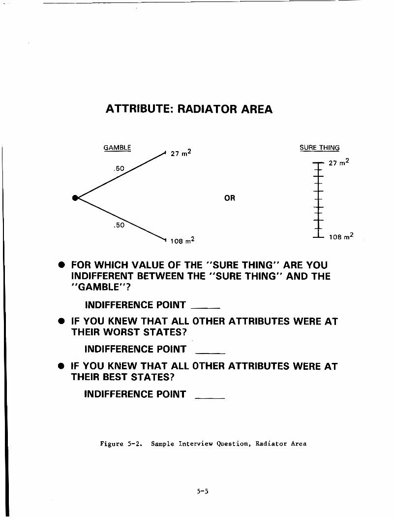
ATTRIBUTE: RADIATOR AREA

27 rn2

108 m2

OR

SURE THING

27 m2

108 m2

e FOR WHICH VALUE OF THE "SURE THING" ARE YOU INDIFFERENT BETWEEN THE "SURE THING" AND THE "GAMBLE"?

INDIFFERENCE POINT

THEIR WORST STATES?

INDIFFERENCE POINT

e IF YOU KNEW THAT ALL OTHER ATTRIBUTES WERE AT

e IF YOU KNEW THAT ALL OTHER ATTRIBUTES WERE AT THEIR BEST STATES?

INDIFFERENCE POINT

Figure 5-2. Sample Interview Question, Radiator Area

5-5

4r

M

N

0 d N

00

M

N

00 0 rl

M

4r

5-6

LL

. b I

a a

= c w

w z c z !l

z Ei k n I a

s m c

Y

0 * w s &

hl E I- N -

s

U a

W

0 P

0 c

5 d

* c P

z

0 c

N E b N

00

..

s

U z

(3

N

Y)

E 0 d N *

as m

N

N E 00 0 F

(3

.. c cn 0 a s

5- 7

W

5 *d 3 b a, U C H d d m b 0 w

m U m

a, u C a, b a,

4-r a, b PI

n

I4 I In

a, I-l P (D c-c

I

a, SVJ W b

a, p ? ; ? c

h U u c c c a ,

a, W C a J O M a c W m up?; cd

m

m

m

In

In

00

I- I m

a0 I

m

h U 0) w m CA

4

4

m

In

00 \o

In m

I I- hl

hl E

Qo 0 d

I b hl

(D aJ 2 b 0 U m .d a m Pz

In

.j

N

In I-

In

0

b I 00

m

00

I- I 00

m

h U .PI

b 7 U m E:

m V

.rl C c u a, c-c

d

m

In

m

m In

Q\ I m

0

I N

M

h 0 C m

0 E n

In

m

0

In

In

00

I- I In

m

5-8

a, rn ca, O M a c a m a d d

hl

rl

rl

0

A

m

N E c o r n

m h l I-

. .

N E In m

I - I I O m 4

N

03 I

m

h U al

vc a v1

E co 0 rl I I- N

m al

2 $4 0 U a .I4 -0 m er;

0

m

d

\D

03 I *

0 A I cu

h U *rl I+ .d P m .rl I+ a, e: C 80 Id rn a, n

d

0

m

03 VI

* I- I e e

03

b I 03

m

h U -!-I

$4 3 U (d E d m U

.A C s U al P

l-l

d

e4

a,

rl

VI

03 I m

0 l-l I

N

h 2

0 n

5-9

G C a J (d4d

d c d c d a u 3

N

0

rl

N

0

d

C O N

a m 9

- a

N

m o . a l

m m

a

? A

hl a 00 0

00 I m

h u al y-r (d cn

d I I- N

cd aJ 2 b 0 U cd d

2

0

d

hl

m

I- I

m

0 d I N

h u d d d P (d d d

I2 c M .d

i

0

0

rr)

9

al

In

0 d

I m

h U 4 d 4 P (d 3 4

E 3 m

5-10

rl

d

d

m In

al

I- I U

00 I m

h U d 4 d

U 7 a 0 Ll ec

5

O b 4

W

al

0

hl

rl

0

hl

rl

rl

rl

rl

In

h

a3

a

0 rl I In

h U d rl d

(d 3 d 3 b 1

v3

n

rl

rl

rl

\o

m I m

0 rl I

N

h

b ii a”

rl

4

rl

In

In

In

h

A m

a3 I rr)

h U d rl d

d 0 1 a 0 Ll PI

n

5-1 1

Responses to the questions asking interviewees to rank the importance of

The ranking for each group was determined by taking the sum of the each of the attributes are summarized for each group and the entire sample in Table 5-3. individual rankings within that group and placing the lowest sum as first in rank, the next lowest sum second, and so on.

Overall, initial safety and technical maturity were most important, and radiator area and cost least important (see also Table 5-4). to note that some individuals ranked safety much lower than other attributes. This was due (primarily) to the perception that safety is a secondary issue (or non-issue) until it can be shown that the system is technically feasible. The mission analysis area (representing users to some extent) was less inter- ested in cost and technical maturity than the more operational attributes like reliability, survivability, and producibility.

It is interesting

Table 5-3. Preference Data from Interviews, Importance of Attributes

Rank Sum Rule Rankings

Attribute Safety Systems Definition Technology Mission Area and Design Area Assessment Analysis

Safety Radiator Area

Des ign Re 1 iab i 1 it y Technical Maturity

Estimated Cost to

Reach Technical

Feas ib i 1 i ty Survivability

Dormancy

Producib i lity

1

7-8

3

2

7-8

5 6

4

6- 7

4-5 6-7

4-5

2-3

6-8

2-3 1

6-8

5

6-8

4

1

4-6

2-3 7-8

7-8

4-6 4-6 2-3

5-12

Table 5-4. Ranking of Attribute Importance

Number of Times Rated

Attribute Most Imp0 rt an t Least Important

Safety 7 1 Radiator Area

Design Reliability

0

0

4

0

Technical Maturity 4 0

Estimated Cost to Prove Technical Feasibility

Surv ivab i 1 it y Dormancy

Produc ib ility

5 0

2

1

5-13

SECTION VI

RANKING ANALYSIS AND DISCUSSION

A. OVERVIEW OF THE DECISION ANALYSIS RESULTS

The results of 11 successfully conducted interviews were analyzed by several different methods. Preference data were elicited from the interviewees on eight attributes for use in a multiattribute decision-analysis model.

The 11 interviews were classified into four areas, with three to four interviews in a group. individual.

The mission analysis area was represented by one The four areas were generically classified as:

Group 1: Safety

Group 2: Systems Definition and Design

Group 3: Technology Assessment

Group 4 : Mission Analysis

The rankings were developed by interviewee and by group. Three group decision rules were used for the groups: Bargaining Rule, and ( 3 ) The Rank Sum Rule.

(1) The Additive Rule, (2) The Nash

B. MATEUS COMPUTER RUNS

A total of 40 MATEUS (MultiATtribute Evaluation of Utilitiez) runs were made to calculate preferences froFthe data of the multiattribute decision analysis interviews. The MATEUS Computer Program is given in Appendix B. The runs calculated both individual and group preferences. ted the preferences for a single group and for each of the interviewees of that group. The 40 MATEUS runs were composed of four runs of the nominal data and twelve variations (three runs each) on the nominal data. Comparable runs for the fourth group were not made because only one individual represented that group. However, a fourth run was included using the baseline nominal data (see Set 1 below).

A single run calcula-

The 40 runs, in sets of three for the three groups, are identified as follows :

(1) Set 1 is the set of runs with the nominal data and are referred to as the NOM/5/MULT Set. The attribute scaling constants are determined with the other attributes set at nominal states, 5 points are used for the piece-wise linear fit to the attribute utility functions, and the multiplicative form of the Keeney-Raiffa methodology is used.

6-1

Set 2 is identified as the NOM/5/LIN Set. Set 2 is identical t o the NOM/5/MULT Set (Set 11, except that the attribute scaling constants are normalized so that their sum is 1.0, and the Linear Form of the Keeney-Raiffa methodology is used.

I 6-2

Set 3 is identified as the NOM/3/MULT Set. Set 3 is identical to the NOM/5/MULT Set (Set 11, except that a 3-point fit rather than a 5-point fit is used for the piece-wise linear fit to the attribute utility functions.

Set 4 is identified as the WORST/3/MULT Set. Set 4 is identical to the NOM/3/MULT Set (Set 31, except that the attribute utility functions were elicited with the other attributes set at their wors t stat e s . Set 5 is identified as the BEST/3/MULT Set. Set 5 is identical to the NOM/3/MULT Set (Set 31, except that the attribute utility functions were elicited with the other attributes set at their best states . Set 6 is identified as the SAFETY Set. Set 6 is identical to the NOM/S/MULT Set (Set l), except that the attribute state for safety (Attribute fl) is fixed at 3 for all systems. of fixing an attribute at its worst state is to remove it, and its contribution, from the analysis. This reveals the sensitivity of the rankings to the attribute.

The effect

Set 7 is identified as the RADAREA Set. Set 7 is identical to the NOM/5/MULT Set (Set 11, except that the attribute state for radiator area (Attribute 4/21 is fixed at 108m2 for all systems.

Set 8 is identified as the DESREL Set. Set 8 is identical to the NOM/5/MULT Set (Set l), except that the attribute state for design reliability (Attribute 113) is fixed at 2 for all systems.

Set 9 is identified as the TECHMAT Set. Set 9 is identical to the NOM/5/M€JLT Set (Set 11, except that the attribute state for technical maturity (Attribute 1/41 is fixed at 3.8 for all systems.

Set 10 is identified as the FEASCOST Set. Set 10 is identical to the NOM/5/MULT Set (Set 11, except that the attribute state for estimated cost to prove technical feasibility (Attribute 1/51 is fixed at $240 million for all systems.

Set 11 is identified as the SURV Set. Set 11 is identical to the NOM/5/MULT Set (Set 11, except that the attribute state for survivability (Attribute 116) is at 5 for all systems.

Set 12 is identified as the DORMANCY Set. Set 12 is identical to the NOM/5/MULT Set (Set l), except that the attribute state for dormancy (Attribute 7) is fixed at 2 for all systems.

(13) Set 13 is identified as the PRODUC Set. Set 13 is identical to the NOM/5/MULT Set (Set l ) , except that the attribute state for producibility (Attribute 8) is fixed at 3 for all systems.

C. MULTIATTRIBUTE RESULTS FOR NOMINAL ATTRIBUTE DATA

Preference data was elicited from the interviewees on eight attributes for use in a multiattribute decision analysis, with twelve variations on the nominal data to examine the robustness of the multiattribute states on the rankings. The methodology for the multiattribute decision analysis model is the Keeney-Raiffa Methodology, which is discussed in Section 11. Section VI discusses the multiattribute results specifically for the nominal data. The nominal data is defined to be the data gathered in the interviews with the 5-point piece-wise linear fit to the interviewee utility functions, the scaling constants determined with the other attributes at nominal states, and the alternative system data unmodified (Set 1: NOM/5/MULT).

Table 6-1 gives the rankings for the system concepts for all 11 interviewees for Set 1 (NOM/5/MULT). Table 6-1 shows that the heat-pipe thermoelectric reactor systems (HTEP, HTEPa) were preferred followed by the heat- pipe Stirling (HSH) system and then a split over the in-core thermionic (ICT) versus the heat-pipe out-of-core thermophotovoltaic (HOCTP) for fourth place. The liquid-metal thermoelectric (LTEP) and Stirling (LSH) are next followed by the heat-pipe AMTEC (HAP). Brayton (LBO), liquid-metal Rankine (LRL), and gas-cooled Brayton (GBH) system.

The least preferred systems are the liquidmetal

When the individual rankings are aggregated into group rankings, the rank order becomes somewhat more apparent. structed from the results of the three group decision rules. thermoelectrics (HTEP, HTEPa) still rank first followed by the heat-pipe Stirling (HSH), the in-core thermionic (ICT) and heat-pipe out-of-core thermionic (HOCTP). The least preferred systems are still the liquid-metal Brayton (LBO), liquid-metal Rankine (LRL), and gas-cooled Brayton (GBH).

See Table 6-2, which was con- The heat-pipe

Table 6-3 gives the rank ordering for the alternative systems according to each of the eight attributes. Each of the attributes was varied in developing the designs that determined the attribute states of the sixteen alternative systems. It is not apparent from Table 6-3 that any one of the attributes can account for the multiattribute results with the nominal data. design reliability, survivability, dormancy, and producibility appear to have the greatest effect in the contributions to the upper-level rankings.

D. RESULTS OF VARIATIONS ON MULTIATTRIBUTE NOMINAL DATA

Runs with thirteen variations on the multiattribute nominal data (Sets 2 through 13) were made to examine the variations of the results to the multiplicative model form, to the preferences of the interviewees, and to the specified states of the alternative systems. will be discussed because the variations are all of second order, and the group decision rules best summarize the variations in the rankings. comparisons are summarized in Tables 6-4a, b, and c.

Only the group decision results

The

6- 3

Table 6-1. Rankings for All Individuals for Set 1 (NOM/5/MULT)

Area la Area 2 Area 3 Area 4

Interview No. System 5 10 2 1 8 6 9 4 7 3 11 Concep tb

LOCTP 10 11 10 9 12 10 13 11 8 12 12 ~~

LBO 14 13 14 14 14 13 14 14 14 14 15

LSH 7 8 8 5 8 5 7 8 6 6 11 ~

LRL 13 15 15 13 15 14 15 13 13 15 14

LAP 12 14 13 11 13 12 12 12 12 13 13

LTE P 5 4 5 6 1 0 6 4 6 4 8 9

GBH 16 16 16 16 16 16 16 16 16 16 16

HOCTP 4 5 6 7 4 7 6 4 7 5 4 ~

HBO 9 9 7 1 0 6 8 9 9 10 9 5

HS H 2 2 3 3 3 2 3 3 5 3 3

HRL 11 11 11 12 9 11 10 7 11 11 6

HAP 8 8 9 8 7 9 5 5 9 7 7

HTPVP 15 15 12 15 11 15 11 15 15 10 8

HTE P 3 - 3 2 2 2 3 2 2 2 2 2

HTEPa 1 1 1 1 1 1 1 1 1 1 1 ~~

ICT 6 6 4 4 5 4 8 1 0 3 4 10

aSee page 6-1 for group names. bSee Table 4-1 on page 4-2 for system names.

6-4

c e t l i r 0

m

N I a

cn

1 I

I

I

I

I

I

I

I

I

0)

a Y KE

a

.4

d a Y 0) E v .* .d cl

U

d

N

m i

I N d

aD

m

m

\o d

e m

N .d

VI d I U 3

e

U d

I m d

3 3

c oc .d m QI n

VI

3

N

m 3

I m d

aD

0 3

m

m

00

U

\D 3

- I U

N d

U ,-I

I m 3

I \o

In 3 I

U 4

3 d

%&l u c 0 0 )

3 E O m c m s0) v m r”t

6- 5

Table 6-3. Rankings by Each of Eight A t t r ibu te s

~ ~~~ ~~ ~

Rad. Design Tech. Feas. System Safety Area Reliab. Maturity Cost Surviv. Dorman. Prod.

LOCTP 9-14 6- 7 4-6 13-14 1 2 7-10 10-14 6- 7

LBO 9-14 14 10 6- 7 13 11-13 10-14 12-14

LSH 9-14 3-4 7-9 1-2 3-4 7-10 10-14 8-1 1

LRL 9- 14 1-2 14-15 8-10 7 14- 16 15-16 15-16 ~~~ ~~ ~ ~~

LAP 9-14 9-10 14-15 8-10 1-2 11-13 15-16 8-1 1

LTEP 9-14 12-13 3 5 8 4- 6 9 1-3 ~~

GBH 16 8 16 ~

16

HOCTP 1-8 6-7 4-6 13-14 14 4- 6 6-8 6- 7

HBO 1-8 15 7-9 6-7 11 7-10 6-8 12-14

HSH 1-8 3-4 4-6 1-2 3-4 4-6 6-8 8-1 1

HRL 1-8 1-2 11-13 8-10 9 11-13 10-14 15-16

HAP 1-8 9-10 11-13 11 1-2 7-10 10-14 8-11

HTPVP 1-8 16 11-13 15 16 14-16 4-5 4-5

HTE P 1-8 11 1-2 1 2 5-6 1-2 1-3 1-3

HTEPa 1-8 12-13 1-2 4 5-6 1-2 1-3 1-3

I CT 15 5 7-9 3 10 3 1-3 4- 5

6-6

\o

d

N

N r(

r.

0 d

m

m

In

U

9 d

rr\

Q

c) d

n -I

n

0 4

4 -I

-I

5 2 7 e

. 4 r)

'J m

d

N

In 4

U

N d

I d

d

P m

0 d

r.

e r(

In

N

I d

d d

U 3

\o

0 d

m

. -4 m- 3

2" ;E .w $ 3 . 9

U

3

N

m d

r. I In

0 - m N

U

r. In

rc d

r. In

d d

U d

03

In d

N d

.N + E?"

:i . 2 m 2 g n d

r.

I

N

In d

m I-

d 4

m

0 I

QI

d

\o

In

\c d

U

N 4

U d

I 0 d

In

0 d

0 d

m

. :N

5 w

28 hi . 4 . Y

6- 7

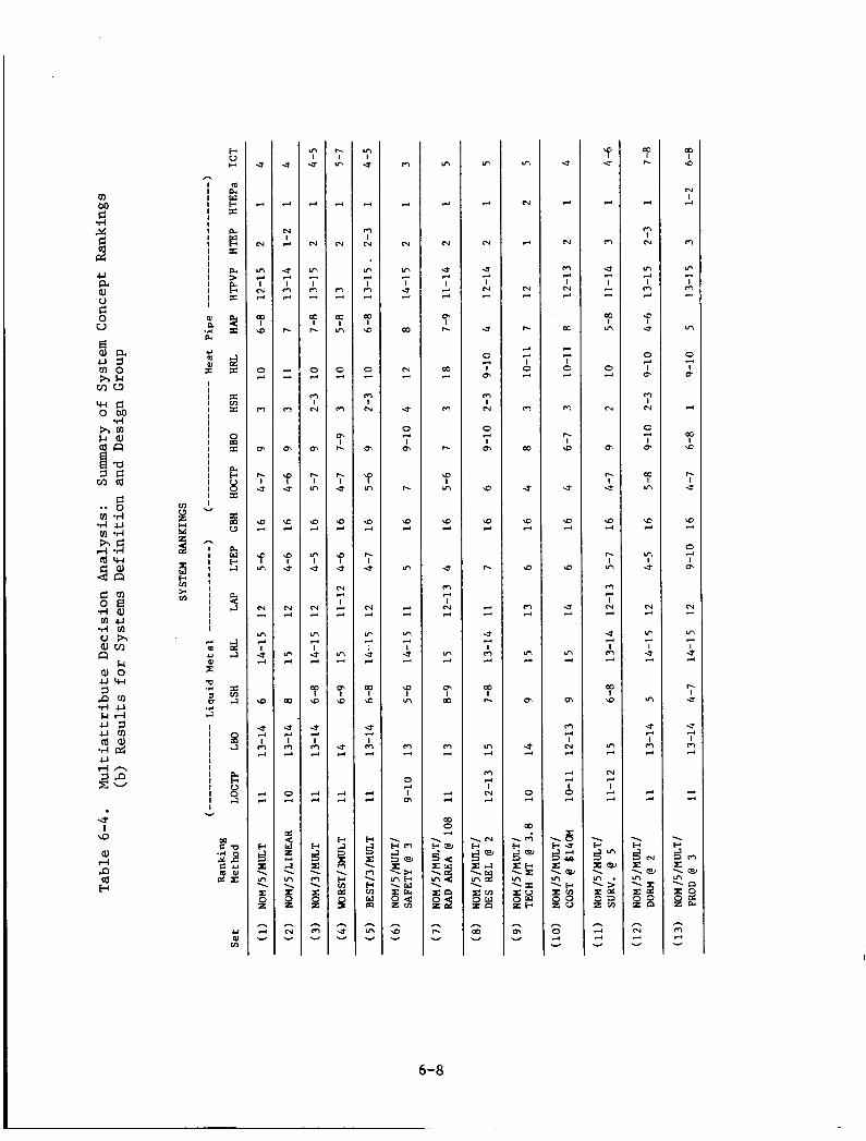
.. g m -rl

u

e I

\o

a, rl P a I3

c V w

h

1 4

i & i z I z I

1 2

I I & I >

I Z I F

I I

$ d 2" u c . 1

U

3

N

m d

I N 3

00

\o

0 3

m

m

r.

U

\o 3

'f m

N 3

m d I

2

2 0 3

d d

s z \ In 1

s z n d W

U

3

N I 3

U d I 0 d

I-

d 3

0

m

\o

U

rc d

\o

U

N d

m d

03

U d I 0 r(

0 3

4 w z c.l

a \ In 1

P h

W pll

In

U

3

N

y.) 3

I m 3

m r.

0 3

0

N

m

r. m

\o d

m *

N 3

m d I

2 m \o

s m 3

d 3

2 X \

m \ z P - m v

r. Ln

3

N

m 3

m m

c 3

m

m r.

r.

U

\o d

'p U

N d

I 3 3

m d

m .D

U d

d d

c 2

z m \

a

E s cz

n 4 W

m U

d

m N

m 3

I m 3

m

0 3

m N

m

'f m

\o 3

r.

U

N d

m .? 4 $4

m \o

U 3

I m d

d d

s z \

0 \ c, m W Q

n m W

m

d

N

m d

I U 3

m

N d

U

0 3

m

r.

\o d

m

3 3

m 3 I

2 \o

m

m d

0 I 3

m

1 w m c.1 a w 4 r

8 % Inc \ W

z m

n .D W

m

d

N

U 3 I 3 3

m r.

m d

m

r.

\o

m

\o d

U

m 3 I N 3

In d

m m

0 3

d 3

m 0

W W

d \

\ $ 2 m \ =La P d n rz v

m

3

N

U 3 I

N 3

U

0 3

m

m N

0 3

m

\o

\o 3

r.

3 3

* 3

I m d

m r.

m 3

m d I N d

\ N

2 - 5 ; In

$ i \

h

OD v

U

3

N

0 3 I

N d

oc

3 3 I 0 d

m

r. \o

U

\o d

\o

* 3

m r(

m

m 3 I N 3

d d I 0 3

18 $2

Pt,

e*

z 1 w

g g h

0 3 v

\o

U

d

m

U I 3

3 3

00

m

0 3

N

m

r.

U

2

r. I In

m 3 I hl d

U d

I m d

m \o

m 3

N 3

I d

d

\

Lim z w

Z d

\

P; PZ n d 4 v

m r.

3

m N

Ln 3

m d

a * 0 3

0.

0

N

0 3

m

m m

.D d

m U

N 3

lP 3 I U d

m

U 3 I m d

d d

\ w z d N

1 3 P B

\ w In

h N 3 w

m \c1

N I 3

m

m 3

I m e

m

0

I m 3

3

m a

r. I *

\o d

0 d I m

N d

m 3 I 2

r.

U

* 3

m 3

d i

\ t,

I: 9.- 1@ In \ a

E h m 3 W

6-8

6 .. m

1 \D

al I4 P (d E-l

n

I

I

I

0)

.d a

m

n

U

e .- I

I I I I I

I 1

I

I I

I

I v

n I

I

I 1 I I I

I I

d 4 &I P) E a .a 3 0. .d

cl I

I

1

I I I I I I v

U

9

I-

N

In d

1 m d

h

2

m

m

? U

\o 4

'f -3

N d

s m d

m 9

In d I ::

r( r(

H -1 a

n z

4

2 . -4 4

4

U

r

N

U

I (CI 3

3

03

m

d d I 0 d

m

P h

m I-

\o 3

U

N d

In d

a \o

U d

I m d

0 d

CO 0

4,

d . !C 5 8 2 4

53 . . 4

a U

r

CI

U r

I P- r

I.

U

C c

F I N

Q1

m U

\o d

VI

U

N d

U d I 0 d

h

\o

In d

I U d

4 A

. 4

J V I

? m 2; $ 5 c v ) . -4 -4 .

U

&

m

In d

U d

I-

* 0

I m d

N

s' m

m h

d

Q.

\o

N d

r? d

In

U

In d

s

d d

. 4

$0

5 ,

!$ -0 E O

T 9 -4 .

6-9

The data for Set 2 (NOM/5/LIN) were derived from the data of Set 1 (NOM/5/MULT) by normalizing the sum of the attribute scaling constants to 1.0 for all interviewees. This reduces the Keeney Multiplicative Form to the Linear Form, where the attributed scaling constants are simple weighting factors, and the multiattribute model is just the weighted sum of the attribute utilities. Linearizing the model makes a significant difference in the form of the model because the sum of the attribute scaling constants for the nominal data for the 11 interviewees range from a low of 2.70 (master scaling constant = -0.9657911 to a high of 4.80 (master scaling constant = -0.999696) with a mean value of 3.516. Even with this significant change in the scaling constants, the results prove to be very robust, with very little change in ranking as shown in Table 6-4.

The data for Set 3 (NOM/3/MULT) were derived from the data of Set 1 (NOM/5/MULT) by using only the end points and the midpoint of the attribute utility functions. The results of using Set 3 serve two purposes: (1) to examine the sensitivity of the results to the coarseness of the piece-wise linear approximation to what is almost certainly a smooth function, and ( 2 ) to use as a reference for examining the results from using the data of Set 4 and Set 5. The results of using the data for Set 3 are shown in Table 6-4. The results of using the data for Set 3 are virtually identical to the results of using the data for Set 1, with only small changes in ranking for a few applications of the group decision rules.

The data for Set 4 (WORST/3/MULT) were derived from the interview data, using the attribute utility functions obtained when the interviewees were asked to assume that all other attributes were at their worst states. Placing the other attributes at their worst states made some of the alternative systems so undesirable that some interviewees were unable to respond with answers that could be translated into attribute utility functions. Where runs could be made to determine rankings with the group decision rules, once again only minor changes in ranking for a few applications of the group decision rules occurred (Table 6-41.

The data for Set 5 (BEST/3/MULT) were derived from the interview data, using the attribute scaling constants obtained when the interviewees were asked to assume that all other attributes were at their best (most-preferred) states. Where runs could be made to determine rankings with the group decision rules, once again only as much as a one-place change in ranking for a few applications of the group decision rules occurred (Table 6-4). Thus the results for Set 4 (WORST/S/MULT) and Set 5 (BEST/3/MULT) indicate that the assumptions made by the interviewees about other attribute states when assessing a utility function for an attribute did not significantly affect the rankings, at least at the group decision level of aggregation.

Several variations on the nominal data were made to examine the effects of specific attributes on the rankings. derived from Set 1 (NOM/5/MULT) by fixing the attribute state for safety (Attribute #1) at 3 for all systems. The results are shown in Table 6-4. results are essentially identical to the results for Set 1, thus eliminating the difference in safety as a sole factor in determining the rankings.

The data for Set 6 (SAFETY) were

The

The

6-10

in-core thermionic (ICT) rises 2 places because i t i s no longer pena l ized f o r a (h igh ly weighted) s a f e t y r a t i n g of 6. The l i q u i d cooled out-of-core thermionic (LOCTP) drops 2 p l a c e s because i t s h ighe r s a f e t y r a t i n g supported i t s somewhat lower sco re on t h e o t h e r a t t r i b u t e s . With s a f e t y removed, i t dropped i n t h e rankings.

The d a t a f o r Se t 7 (RADAREA) were der ived from S e t 1 (NOM/5/MULT) by f i x i n g t h e a t t r i b u t e s t a t e f o r r a d i a t o r area ( A t t r i b u t e #2) a t 108m2 f o r a l l systems. The r e s u l t s are shown i n Table 6-4. The heat-pipe Brayton (HBO) and heat-pipe thennophotovol ta ic (HTPVP) r ise 2 p laces s i n c e t h e i r l a r g e r a d i a t o r areas no longer pena l i ze them. r e s u l t s f o r S e t 1, thus e l i m i n a t i n g the d i f f e r e n c e i n r a d i a t o r a r e a as t h e s o l e f a c t o r i n determining t h e rankings.

The r e s u l t s are e s s e n t i a l l y i d e n t i c a l t o t h e

The d a t a f o r Se t 8 DESREL were der ived from Se t 1 (NOM/5/ MULT) by f i x i n g t h e a t t r i b u t e s t a t e f o r des ign r e l i a b i l i t y ( A t t r i b u t e #3) a t 2 f o r a l l sys t ems . The r e s u l t s are shown i n Table 6-4. The r e s u l t s are e s s e n t i a l l y i d e n t i c a l t o t h e r e s u l t s f o r S e t 1, t h u s e l imina t ing t h e d i f f e r e n c e i n des ign r e l i a b i l i t y as t h e s o l e f a c t o r i n determining t h e rankings.

The d a t a f o r Se t 9 (TECHMAT) were der ived from S e t 1 (NOM/5/MULT) by f i x i n g t h e a t t r i b u t e s t a t e f o r technica l ma tu r i ty ( A t t r i b u t e # 4 ) a t 3.8 f o r a l l systems. The r e s u l t s are shown i n Table 6-4. The r e s u l t s a r e e s s e n t i a l l y i d e n t i c a l t o t h e r e s u l t s f o r S e t 1, except t h e heat-pipe the rmoe lec t r i c s (HTEP, HTEPa) r eve r se o r d e r and t h e l iquid-metal cooled S t i r l i n g (LSH) drops 3 posi- t i o n s because i t l o s e s i t s h igh advantage i n t e c h n i c a l ma tu r i ty con t r ibu t ion .

The d a t a f o r Se t 10 (FEASCOST) were der ived from Se t 1 (NOM/5/MULT) by f i x i n g t h e a t t r i b u t e s t a t e f o r c o s t ( A t t r i b u t e #5) a t $240 m i l l i o n f o r a l l systems. The r e s u l t s are shown i n Table 6-4. The r e s u l t s a r e e s s e n t i a l l y i d e n t i c a l t o t h e r e s u l t s f o r Se t 1, except f o r t h e l i q u i d - m e t a l S t i r l i n g (LSH) which drops t h r e e p l a c e s because it loses i t s advantage of having a r e l a t i v e l y low c o s t while t h e heat-pipe Brayton (BO) r i s e s i n t h e rankings due t o i t s pena l ty f o r a somewhat high c o s t .

The d a t a f o r S e t 11 (SURVIV) were der ived from S e t 1 (NOM/5/MULT) by f i x - ing t h e a t t r i b u t e s t a t e f o r s u r v i v a b i l i t y ( A t t r i b u t e f 6 ) a t 5 f o r a l l systems. The r e s u l t s are shown i n Table 6-4. L i t t l e change i s observed, even f o r t h e low s u r v i v a b i l i t y systems because they tend t o have o t h e r low a t t r i b u t e va lues holding them down i n t h e rankings.

The d a t a f o r S e t 12 (DORMAN) were der ived from S e t 1 (NOM/5/MULT) by f i x i n g t h e a t t r i b u t e s t a t e f o r dormancy ( A t t r i b u t e #7) a t two f o r a l l systems. The r e s u l t s a r e shown i n Table 6-4. The in-core thermionic (ICT) drops i n p o s i t i o n when dormancy i s removed because i t s h igh s c o r e ( a 10) i s removed.

The d a t a f o r Se t 13 (PRODUC) were der ived from S e t 1 (NOM/5/MULT) by f i x i n g t h e a t t r i b u t e s t a t e f o r p roduc ib i l i t y ( A t t r i b u t e 1 8 ) a t t h r e e f o r a l l systems. The r e s u l t s are e s s e n t i a l l y i d e n t i c a l t o t h e r e s u l t s f o r S e t 1, except f o r t h e l i q u i d - m e t a l cooled thermoelec t r ic (LTEP) , which drops t h r e e p o s i t i o n s i n t h e ranking because it relies heav i ly on i t s high p r o d u c i b i l i t y f o r i t s p o s i t i o n .

6-11

I E. GENERAL CONCLUSIONS

I F. CRITIQUE OF MULTIATTRIBUTE DECISION ANALYSIS METHODOLOGY

The general conclusions can be made from Table 6-4, which summarizes the results from the application of the group decision rules to the baseline data of Set 1 (NOM/5/MULT). All other runs resulted in only minor variations on the rankings of Table 6-4 . thermoelectrics (HTEP, HTEPa). The third place ranking usually went to the heat-pipe Stirling (HSH), followed by fourth and fifth place with the in-core thermionic (ICT) and heat-pipe out-of-core thermionic (HOCTP). Sixth through tenth place went to the liquid-metal thermoelectric (LTEP) and Stirling (LSH), followed by the heat-pipe AMTEC (HAP), Brayton (HBO), and Rankine (HRL). The least preferred systems were the liquidmetal out-of-core thermionic (LOCTP) liquid-metal AMTEC (LAP), heat-pipe thermophotovoltaic (HTPVP), liquid-metal Brayton (LBO) and Rankine (LRL), and the gas-cooled Brayton (GBH).

First and second rankings always went to heat-pipe

Variations on the baseline data of Set 1 (NOM/S/MULT), as made in data Set 2 through Set 5, made at most a two-place change in the rankings as determined by the group decision rules, with typically no change. Data Set 6 and Set 13 fixed each of the attribute states and made changes in the ranking as compared to the baseline data of Set 1 (NOM/5/MULT) of as much as three places in ranking. (ICT) by 2 places because of a lower safety rating on that system, which was not counted against it in Set 11. Data Set 7, where radiator area is dropped as an attribute, improved the heat-pipe Brayton and heat-pipe thermophotovoltaic (HTPVP) by two places due to their large radiator areas. Data Set 9, where technical maturity is dropped, causes the liquid-metal Stirling (LSH) to drop three places due to its high reliance on technical maturity. The liquid- metal Stirling (LSH) also relies on low cost for a high ranking. When cost is eliminated as an attribute, as in data Set 10, the liquid-metal Stirling drops three places in the rankings. In data Set 13, where producibility is dropped, the liquid-metal cooled thermoelectric (LTEP) drops three places due to its reliance on high producibility in the scoring.

Data Set 6 improved the preference for the in-core thermionic

It was not possible to rank the alternative systems on the basis of any one attribute.

In summary, the top three rated systems were virtually unchanged with all twelve variations in assumptions across groups. trics (HTEP, HTEPa) and heat-pipe Stirling (HSH) were the top three systems. Some shifting occurred in the fourth place although the in-core thermionic (ICT) tended to come up most often.

The decision analysis process was viewed as useful for (1) reducing the large number of subsystem combinations to a manageable number; (2 ) characterizing and communicating the alternatives; and (3) providing the rationale and support for R6D planning to carry forward with the more promising technologies.

The heat-pipe thermoelec-

The multiattribute decision analysis methodology was successful in all of the 11 interviews in ranking all the alternative system concepts. The

group decision rules were capable of aggregating preferences by groups, and, in general, the three group decision rules were in agreement.

The multiattribute decision analysis was a deterministic analysis, as contrasted with a probabilistic analysis, and so did not completely reveal the technical experts' opinion as to the attribute states of the alternative systems. had been estimated probabilistically. a Monte Carlo simulation model, using subjectively estimated cumulative probability distributions for the attribute states of the alternative systems, would have been sufficient data for a probabilistic analysis. The present analysis does not incorporate the uncertainties in the attribute state estimates. As a result, the process highlighted the need for more technical information about the systems and the degree of confidence to be placed on such information.

A better analysis could have been undertaken if the attribute states Either a discrete probability tree or

The interview times could have been shortened if only three-point rather than five-point estimates had been made of the attribute utility functions. With the worst-state and the best-state used for two of the three points, questions for only one-attribute utility value need be asked in the interviews. Comparison of Tables 6-1 and Table 6-4 show that only minor differences in the rankings would have resulted in the group decision rules. and monotonicity of preferences can be assumed for the attribute states, an attribute utility function of the "constant risk aversion'' form:

Because continuity

u(x> = a + beCX

would have sufficed. Given the high premium for short interview times, it is recommended that in the future, unless there is strong reason to believe that the utility function is not represented by such a function with sufficient accuracy, the attribute utility functions be derived from three-point estimates.

It was difficult for some, and impossible for others, of the interviewees to assess gambles with respect to the set of attributes at their worst states. Had the system concepts been determined further in advance, the attribute worst states could have been made more desirable. It is highly recommended, in future multiattribute decision analyses, that the system states be determined before the interviews are conducted. This will also preclude the unfortunate situation in which the system states are ultimately determined to lie outside the range of the assessed attribute states.

During the course of the process, the need for displaying the source calculations of the rankings was identified. Forays into piles of computer listings, no matter how comprehensive, were deemed insufficient. Although such transparency can be shown to some extent with summary graphics, an interactive version of the model to allow display of both intermediate and summary calculations is needed.

6-13

SECTION VI1

CONCORDANCE OF RANKINGS

A. INTRODUCTION

This section presents and discusses the results of concordance calculations for the rankings presented in Section VI (see subsection C in Section I1 for a discussion of concordance statistics). dances were calculated and analyzed:

Two different types of concor-

(1) Individual rankings within groups.

( 2 ) Group rankings with different group decision rules.

The purpose of these concordance calculations and analyses was to ascertain how robust, or conversely, how sensitive the rankings were to: differences among individuals within groups and differences in group decision rules. general, the rankings were highly concordant across individuals within groups and across different group decision rules, implying that the rankings presented in Section VI were indeed robust.

In

The concordance of the rankings given to the sixteen alternative system concepts by individuals within the three groups was examined in two ways: (1) by comparing the individual rankings within groups (Table 7-11 for each of the 40 runs previously described in Section VI; and ( 2 ) by comparing the group rankings according to the additive, Nash, and rank sum rules (Table 7-21. The following observations can be made:

There is not, of course, perfect agreement throughout the ranking.

There are several instances in which the ranks assigned to several alternatives by one interviewee in a group seem to be at variance from those given by the other interviewees in the group.

The concordance measures in every instance, however, are highly significant. Each of them is significant well below the 1% level; many are significant below the 0.1% level.

Accordingly, by each of the comparison methods, there is substan- tial agreement as to the rankings of the sixteen alternative systems within each of the three groups of interviewees.

The chi-square values corresponding to the coefficients of concordance indicate no instances in which there is no significance at a minimum 1% level. The other 78 chi-square values are significant well beyond the 5% level. This indicates excellent agreement among interviewees and among group decision rules. Although it is possible to examine concordance among different methods, this was not done, due to time constraints. The majority of lower concordance values occurred within Group 2 - Systems Definition due to different weightings of certain attributes which have moderate impacts (cost, design reliability, survivability, producibility) on ranking.

7-1

Table 7-1. Summary of Kendall's Coefficient of Concordance (W) and the Associated Chi-square Values (X2) for all Runs: Within Groups

Individuals

1 2 3

RUNS METHOD W X2 W X2 W X2

1-3 5- 7 9-1 1

17-19 21-23 25-27

NOM/ 5 /MULT NOM/ 5 / LIN NOM/ 3 /MULT

WORST/ 3 /MULT BEST/3/MULT

NOM/ 5 /MULT SAFETY @ 3 NOM/ 5/MULT RAD AREA @ 108

NOM/ 5 /MULT DES REL @ 2

NOM/ 5 /MULT TECH MT @ 3.8

NOM/ 5 /MULT COST @ $240M

NOM/ 5 /MULT SURV @ 5

NOM/5/MULT DORM @ 2

NOM/ 5 /MULT PROD @ 3

0.9596 57.57 0.9750 58.50

0.9647 57.88

0.9588 43.15 0.9647 57.88

0.9314 0.9366

0.9294

0.8725 0.9268

41.91

42.15

41.82

39.26 41.71

0.9072 0.9784

0.9327

0.9046 0.9242

40.82 44.03

41.97

40.71 41.59

0.9784 44.03 0.9665 57.99 0.9647 43.41

29-31 0.9732 58.39 0.9163 41.24 0.9092 40.91

33-35 0.8908 40.09 0.9449 56.69 0.8556 38.50

37-39 0.9246 55.48 0.9144 41.15 0.8974 40.38

41-43 0.9621 57.73 0.8791 39.56 0.9131 41.09

45-47 0.9137 41.12 0.9441 56.65 0.8693 39.12

49-51 0.9346 42.06 0.9399 42.29 0.9511 57.07

53-55 0.9408 56.45 0.8876 39.94 0.9229 41.53

7-2

Table 7-2. Summary of Kendall's Coefficient of Concordance (W) and the Associated Chi-square Values (X2) for all Runs: Decision Rules

Group

1 2 3

RUNS METHOD W X2 W X2 W X2

1-3

5-7

9-1 1

17-19

21-23

25-2 7

29-31

33-35

41-43

45-4 7

49-51

53-55

NOM/5/MULT NOM/5/LIN

NOM/3/MULT

WORST/3/MULT

BEST/3/MULT

NOM/5/MULT SAFETY @ 3

NOM/S/MULT RAD AREA @ 108

NOM/5/MULT DES REL @ 1

NOM/5/MULT COSTS @ $240M NOM/5/MULT SURV @ 5

NOM/5/MULT DORM @ 2 NOM/5/MULT PROD @ 3

0.9987 44.94 0.9984 44.93

0.9987 44.94 0.9922 44.65

0.9980 44.91

0.9974 44.88

0.9984 44.93

0.9948 44.76

0.9935 44.71

0.9944 44.75

0.9967 44.85

0.9987 44.94

0.9902 0.9964

0.9895 0.9738

0.9833

0.9971

0.9915

0.9948

0.9971

0.9739

0.9843

0.9774

44.56 44.84 44.53 43.82

44.25

44.87

44.62

44.76

44.87

43.82

44.29

43.98

0.9869

0.9971

0.9889

0.9926

0.9816

0.9969

0.9863

0.9862

0.9817

0.9758

0.9912

0.9859

44.41 44.87

44.50 44.67

44.17

44.86

44.38

44.38

44.18

43.91

44.60

44.37

7-3

SECTION VI11

REFERENCES

1. Keeney, R. L., and Raiffa, H., Decisions with Multiple Objectives: Preferences and Value Tradeoffs, John Wiley, New York, 1976.

2.

3.

4.

5.

6.

7.

8.

9.

10.

11.

12.

13.

"Special Issue on Decision Analysis," IEEE Transactions on Systems Science and Cybernetics (R. A. Howard, Ed.), Vol. SSC-4, No. 3, pp. 199-366, September 1968.

Raiffa, H., Decision Analysis: Introductory Lectures on Choices Under Uncertainty, Addison-Wesley, Reading, Massachusetts, 1968.

Raiffa, H., Preferences for Multi-Attributed Alternatives, RM-5686- DOT/RC, The Rand Corporation, Santa Monica, California, 1969.

Schlaifer, R., Analysis of Decisions Under Uncertainty, McGraw-Hill, New York, 1969.

Boyd, D. W., A Methodology for Analyzing Decision Problems Involving Com- plex Preference Assessments, Decision Analysis Group, Stanford Research Institute, Menlo Park, California, 1970.

Edwards, W., "Social Utilities," The Engineering Economist, Summer Symposium Series, No. 6, pp. 119-129, 1971.

Edwards, W., Guttentag, M., and Snapper, N., "Effective Evaluation: A Decision Theoretic Approach," in Streuning, E. L., and Guttentag, M., Eds., Handbook of Evaluation Research, Beverly Hills, California, Sage Publications, 1975.

Edwards, W., "How to Use Multiattribute Utility Measurement for Social Decisionmaking," IEEE Transactions on Systems, Man, and Cybernetics, Vol. SMC-7, No. 5, pp. 326-340, May 1977.

Fischer, G. W., Four Methods for Assessing Multi-Attribute Utilities: An Experimental Validation, Report 037230-6-T, Engineering Psychology Laboratory, The University of Michigan, Ann Arbor, Michigan.

Gardiner, P. C., and Edwards, W., "Public Values': Multiattribute Utility Measurement for Social Decision Making," Human Judgment and Decision Processes (S. Schwartz and M. Kaplan, Eds.), Academic Press, New York, 1975.

Geoffrion, A. M., Dyer, J. S., and Feinberg, A., "An Interactive Approach for Multi-Criterion Optimization with an Application to the Operation of an Academic Department," Management Science, Vol. 19, No. 4, pp. 357-368, 1972.

Krantz, D. M., et al., Foundations of Measurement, Vol. I, Academic Press, New York, 1971.

8-1

14.

15.

16.

17.

18.

19.

20.

21.

22.

23.

24.

25.

26.

27.

Lee, S. M., Goal Programming for Decision Analysis, Auerback Publishers, Phi lade lphia, Pennsylvania, 1972.

MacCrimmon, K. R., Decision Making Among Multiple-Attribute Alternatives: A Survey and Consolidated Approach, RM-4823-ARPA, The Rand Corporation, Santa Monica, California, December 1968.

Multiple Criteria Decision Making, Vol. 6 of Studies in the Management Sciences (M. K. Starr and Milan Zeleny Eds.), North-Holland Publishing Co., New York, 1977.

Winterfeldt D. V., and Fisher, G. W., Multi-Attribute Utility Theory: Models and Assessment Procedures, Technical Report 011313-7-T, Engi- neering Psychology Laboratory, The University of Michigan, Ann Arbor, Michigan, November 1973.

Multiple Criteria Decision Making: Kyoto 1975, Vol. 23 of Lecture Notes in Economics and Mathematical Systems (M. Zeleny, Ed.), Springer- Verlag, New York, 1976.

"Multiple Criteria Problem Solving: Proceedings, Buffalo, N.Y. ( U . S . A . ) , 1977," Vol. 155 of Lecture Notes in Economics and Mathematical Systems (S. Zionts Ed.), Springer-Verlag, New York, 1978.

Feinberg, A,, and Miles, R. F., Jr., A Brief Introduction to Multi- Attribute Decision Analysis, JPL Internal Document 5030-222, June 1978, reissued as Volume I of JPL Internal Document 5103-47, Decision Analysis for Evaluating and Ranking Small Solar Thermal Power System Technolo- ogies, January 1979.

Brown, R. V., Kahr, A. S., and Peterson, C., Decision Analysis for the Manager, Holt, Rinehart and Winston, New York, 1974.

Winkler, R. L., Introduction to Bayesian Inference and Decision, Holt, Rinehart and Winston, New York, 1974.

von Neumann, J., and Morgenstern, O., Theory of Games and Economic Behavior, John Wiley, New York, 3rd Ed., 1967 (1st Ed., Princeton University Press, Princeton, New Jersey, 1944).

Hadley, G., Introduction to Probability and Statistical Decision Theory, Holden-Day, San Francisco, California, 1967.

Luce, R. D., and Raiffa, H., Games and Decisions, John Wiley, New York, 1957.

DeGroot, M., Optimal Statistical Decisions, McGraw-Hill, New York, 1970.

Fishburn, P. C., Utility Theory for.Decision Making, John Wiley, New York, 1970.

8-2

28.

29.

30.

31.

32.

33.

34.

35.

36.

37.

38.

39.

40.

41.

42.

Keeney, R. L., and Wood, E. F., "An Illustrated Example of the Use of Multiattribute Utility Theory for Water Resource Planning," Water Resources Research, Vol. 13, No. 4, pp. 705-712, August 1977.

Keeney, R. L., "Evaluation of Proposed Storage Sites," Operations Research, Vol. 27, No. 1, pp. 48-64, January-February 1979.

Arrow, K. J., Social Choice and Individual Values, Yale University Press, New Haven, 2nd Ed., 1963 (1st Ed., 1951).

Fishburn, P. C., The Theory of Social Values, Princeton University Press, Princeton, New Jersey, 1973.

Sen, A. K., Collective Choice and Social Welfare, Holden-Day, San Francisco, California, 1970.

Dyer, J. S., and Miles, R. F., Jr., A Critique and Application of Collective Choice Theory: JupiterISaturn 1977 Project, JPL Internal Document 900-777, California, February 1977.

Trajectory Selection for the Mariner

Dyer, J. S., and Miles, R. F., Jr., "An Actual Application of Collective Choice Theory to the Selection of Trajectories for the Mariner Jupiter/ Saturn 1977 Project," Operations Research, Vol. 24, No. 2, pp. 220-224, March-April 1976.

de Borda, Jean-Charles, "Memoire sur les elections au scrutin," Histoire de 1'Academie Royale des Sciences, 1781.

Young, H. P . , I1 An Axiomatization of Borda's Rule," Journal of Economic Theory, Vo1. 9, pp. 43-52, 1974.

Nash, J. F., Jr., "The Bargaining Problem," Econometrica, Vol. 18, pp. 155-162, April 1950.

Harsanyi, J. C., "Cardinal Welfare, Individualistic Ethics, and Inter- personal Comparison of Utility,'' Journal of Political Economy, Vol. 63, pp. 309-321, 1955.

Siegel, S., Nonparametric Statistics, McGraw Hill, New York, 1956.

Feinberg, A . , R. F. Miles, Jr., J. H. Smith, and E. M. Scheuer, Advanced Vehicle Preference Analysis, Volumes I and 11, JPL Document 5030-566, Jet Propulsion Laboratory, Pasadena, CA, September 1983.

Feinberg, A., R. F. Miles, Jr., et al., FBI Fingerprint Identification Automation Study: Final Report, Volume I: Ranking and Sensitivity Analysis, JPL Internal Document 5030-517-1, Jet Propulsion Laboratory, Pasadena, California, December, 1981.

Huber, G. P., Managerial Decision Making, Scott, Foresman and Company, Glenview, Illinois, 1980.

8- 3

APPENDIX A

QUESTIONNAIRE USED FOR INTERVIEWS

A-1

A-3

w

> d w s z

H

W

c4 0

W cn 0

d 3 a

A-4

n

n cn f- z W r: W d

3 W W d

H

-cn- z s

B U

Y

r w f- cn $. VI

d W L 0 a W U

4 a cn

a

z5 Y

n w z z H

a s m

2 s 0

u

A-5

SAFETY

B e s t 10 safety l e v e l exceeds normal s a f e t y exceeds s a f e t y exceeds Case pre-f l ight precaut ions due cu r ren t launch/ cu r ren t d i sposa l

t o na ture of power system f l i g h t standards p rac t i ces / co re w i l l --remains s u b c r i t . disperse safely i n if immersed i n event of r een t ry water

7 low r i s k of exposure i n event low risk of of p r e - f l i g h t acc ident ; problems i n event o b j e c t s reaching safety l e v e l comparable t o of abort--remains t h e ground current practice s u b c r i t i c a l i f

low r i s k of large

immersed i n water

3 some risk of r a d i a t i o n some r i s k of prob- some r i s k of large exposure i n event of pre- f l i gh t acc ident abort t h e ground

lems i n event of objects reaching

Worst 0 pre-f l i g h t acc ident p l aus ib l e scena r ios large rad ioac t ive Case could lead t o c r i t i c a l i t y f o r c r i t i c a l i t y / objects reach t h e

and/or r a d i a t i o n dosage explosion i n event ground t o personnel of water immersion

,very large o b j e c t s reaching t h e ground, o r loss of coolant after deployment

A-6

DESIGN RELIABILITY

B e s t 10 C a s e

8

6

4

2

Worst 0 Case

Very high-tolerant t o single po in t and mu1 t i p l e f a i l u r e s wi th g race fu l degradation I n performance.

H igh- - to l e ran t t o s i n g l e p o i n t f a i l u r e s w i t h g r a c e f u l d e g r a d a t i o n I n performance. T o l e r a n t wi th in c e r t a i n l i m i t s t o mu1 t ip le -poin t failures.

ModerateA: t o l e r a n t to single po in t f a i l u r e s w i t h g race fu l degradat ion i n performance--low risk of s y s t e m f a i l u r e . Moderate t o l e r a n c e t o mu1 t i p l e f a i l u r e s . Moderate-B: more l i m i t e d tolerance t o single po in t f a i l u r e s w i t h more dramatic degradat ion i n system p e r f o r m a n c e o v e r time--some r i s k of sys t em f a i l u r e . Low to l e rance t o mul t ip le f a i l u r e s

Moderate-C: l o w e r t o l e r a n c e t o s i n g l e p o i n t f a i l u r e s and v e r y low t o l e r a n c e t o m u l t i p l e f a i l u r e s with moderate r i s k of system f a i l u r e .

Low-susceptable t o s i n g l e p o i n t f a i l u r e s wh ich p r o p a g a t e I n t o o v e r a l l s y s t e m f a i l u r e ( t h r o u g h l o s s of c o o l a n t or damage t o c o n t r o l sys tem) . S i m i l a r l y , m u l t i p l e f a i l u r e s r e s u l t i n sys t em f a l l u r e .

A- 7

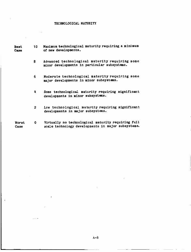
TECHNOLOGICAL MATURITY

Best 10 Case

8

6

4

2

Worst 0 Case

Maximum techno log ica l m a t u r i t y r e q u i r i n g a minimum of new developments.

Advanced t e c h n o l o g i c a l m a t u r i t y r e q u i r i n g some minor developments i n p a r t i c u l a r subsystems.

Moderate t e c h n o l o g i c a l m a t u r i t y r e q u i r i n g some major developments i n minor subsystems.

Some t echno log ica l m a t u r i t y r e q u i r i n g s i g n i f i c a n t developments i n minor subsystems.

Low t e c h n o l o g i c a l m a t u r i t y r e q u i r i a g s i g n i f i c a n t developments i n major subsystems.

V i r tua l ly no t echno log ica l m a t u r i t y r e q u i r i n g f u l l scale technology developments i n major subsystems.

A-8

S U R V I V A B I L I T Y

Best 10

7

3

Wors 0

Very h igh l i ke l ihood of surviving m i l i t a r y threats a t r e q u i r e d l e v e l s and h i g h e r w i t h o u t l o s s of performance. Also a high likelihood of surv iv ing meteor i te impacts without loss of performance.

Likely t h a t system w i l l survive designed l e v e l s of m i l i t a r y threat and meteorite hazard without loss of performance.

Moderate l ike l ihood of surviving designed l e v e l s o f m i l i t a r y th rea t and m e t e o r i t e hazard w i t h o u t loss of performance.

Low l i k e l i h o o d o f s u r v i v i n g m i l i t a r y t h rea t s a t d e s i g n l e v e l s . High r i s k of s y s t e m f a i l u r e in e v e n t of m e t e o r i t e impact o r m i l i t a r y induced damage.

A- 9

beAB -FBttQWfNWDOIWANCY CAPABILITY

B e s t 10

7

3

Worst 0 Case

Mu1 t i p l e restart c a p a b i l i t y t h r o u g h o u t m i s s i o n l i f e t ime w i t h h i g h d e g r e e of load f o l l o w i n g c a p a b i l i t y u s i n g e l ec t r i ca l s w i t c h i n g t o fo l low load c l o s e l y i n s t e p s and r e s p o n d i n g q u i c k l y t o r a p i d d r o p s i n load. Minimal power s t o r a g e requirements for s t a r t u p enabling long per iods of dormancy .

Mu1 t i p l e res t a r t c a p a b i l i t y th roughou t m i s s i o n l ifetime. Moderate power s t o r a g e r e q u i r e d f o r r e s t a r t s due t o power requirements t h u s dormancy per iod is shor t e r t h a n i n b e s t case. Moderate load f o l l o w i n g c a p a b i l i t y due t o gas v a l v i n g system for dumping excess energy.

M u l t i p l e r es ta r t c a p a b i l i t y th roughou t m i s s i o n l i fe . High power r e q u i r e m e n t s f o r s t a r t u p . Reduced l o a d f o l l o w i n g c a p a b i l i t y due t o vapor va lv ing f o r dumping e x c e s s energy.

Poor load f o l l o w i n g c a p a b i l i t y - s y s t e m r u n s a t f u l l power and vents excess heat us ing an unvalved s y s t e m o r one w i t h e l e c t r i c shunt . No dormancy c a p a b i l i t y o t h e r t h a n l aunch p e r i o d p r i o r t o i n i t i a l s t a r t and no a b i l i t y t o shutdown a f t e r s t a r tup .

A-10

B e s t 10 Case

7

3

Worst 0 Case

PRODUCPBILITY/PRACTICALITX

Hig h l y m o d u l a r i z e d i n d epend e n t s u b s y s tem s w i t h simple in t e r f aces . E a s i l y manufactured materials, p a r t s , a n d assemblies a n d no e x t r a o r d i n a r y t o o l i n g / f a c i l i t i e s required. A l l components can b e p r e - f l i g h t t e s t e d i n d e p e n d e n t l y w i t h o u t assembling the whole system.

System i s somewhat m o d u l a r w i t h some complex in t e r f aces . The fabr icabi l i ty is similar t o other spaceb or ne s y s tem s w i t h com parabl e f a b r i c a t i o n problems. The subsystems are, f o r t h e most par t , testable independently.

M i n i m a l modular i ty wi th complex i n t e r f a c e s between most of t h e subsystems. The fabr icabi l i ty is more d i f f i c u l t t h a n comparable s p a c e b o r n e sys tems r e q u i r i n g some s p e c i a l m a t e r i a l s . Some of t h e subsystems are d i f f i c u l t t o test wi thout a vacuum environment.

V i r t u a l l y n o m o d u l a r i ty-system is an i n t e g r a t e d w h o l e w i t h c o m p l e x i n t e r f a c e s . I t i s v e r y d i f f i c u l t t o manufacture s ince special materials, t o o l i n g , and f a c i l i t i e s are r e q u i r e d . Major subsystems are n o t testable and may r e q u i r e space testing t o determine f l i g h t worthiness.

A-11

k

M

- - a

W W ,

c 2

e W 0 z W U W L L

5

E z -

A-12

F a W U : cn W + 3

C c m w

t

k

: W rr

m W

ce: 0

A-13

U 0

O C

L z w O W

1 .

A-14

N E 00 0 r(

c: 0

-1

N E

00 0 rl

e

W

& U 0-

I- z ij e W 0 z w ct W L u, - n 2 I

+ W a a 2i v) W I- 3 P

I- z k U w I I- O d d

e

c z e W 0 2 w Dt W LL L

ij

E z 0

A-15

CL: 0

m .

W c W 0 2

ee: 0

0 .

w I- 3 m - ce: I- k

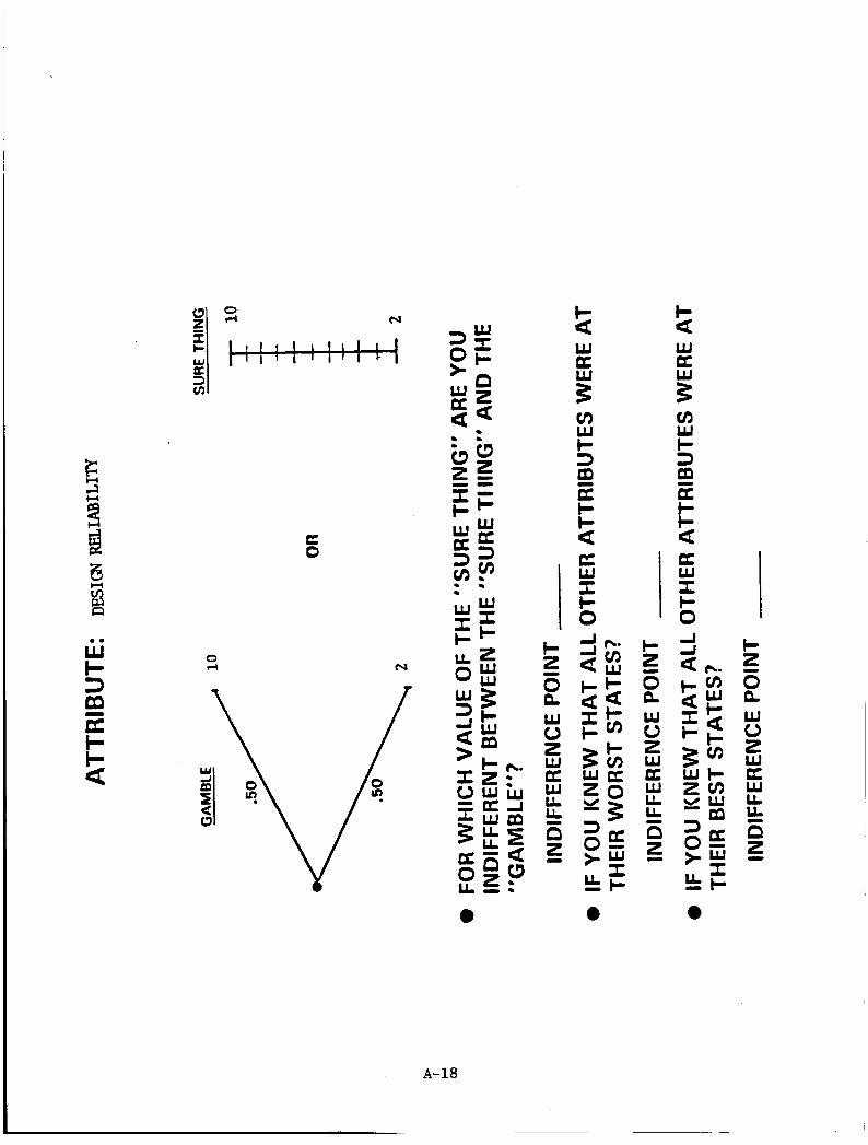
.e

W 0 d

m m m

u 5 O W

k W cc w 9 v) W I- 3

I- I-

p: W

m z a

f z

0

LI- a a Irc

I- 2 0 e W u I W K W L U

-

- P 2 -

k W ce : cn w I- 3

ce I- I-

m - a

I- z e W 0 2 W x W U LL

5

i5 z -

A-18

U 0

2 5 e W 0 2 W U w LL LL i3 3 w

A-19

ir W

e m

W I-

I

I- I

e 5 W 0

w U

A-20

W c 5 m z c c a

E 0

so M

f = CI-

W w , aft

- - a

W W ,

I- 2

e W 0 z W U W LL L

5

Es 2 I

k I- a

m W I- 3 P

I- E

k a W I I- O

A-21

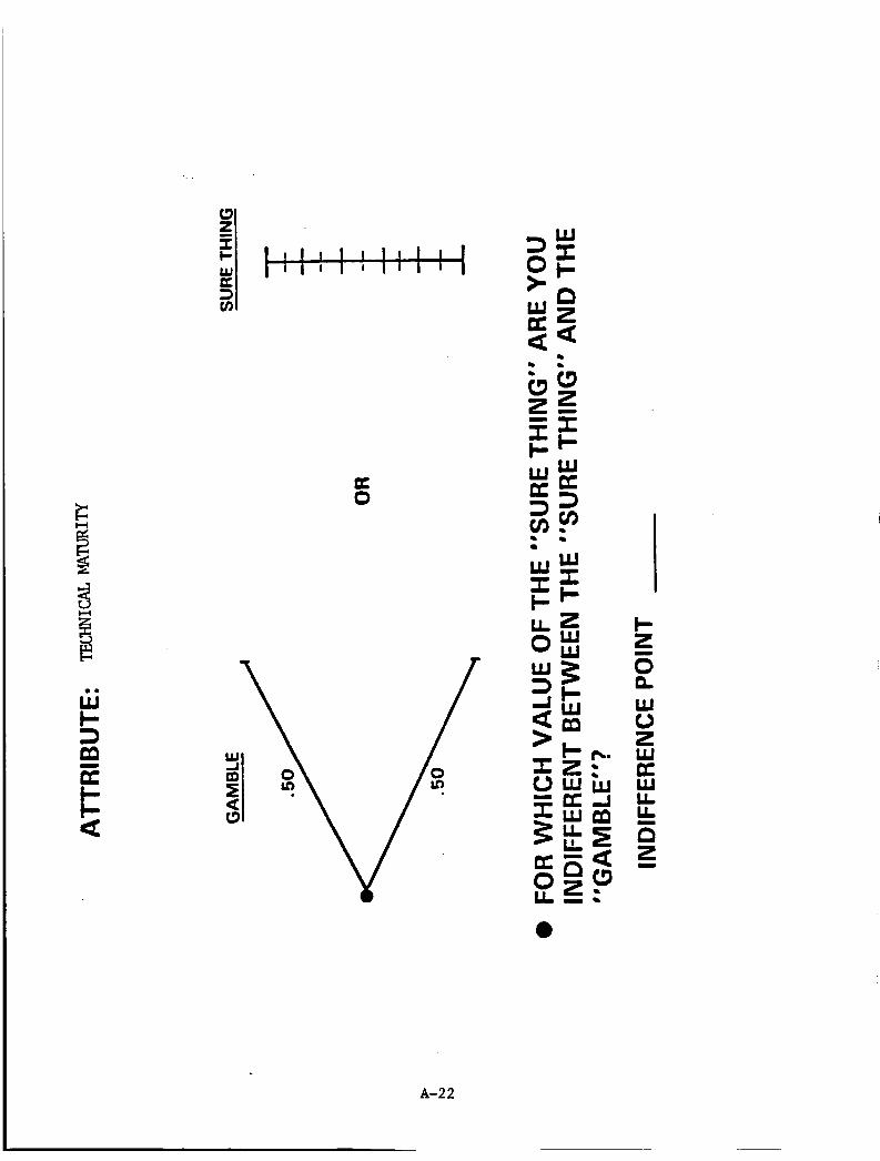
W tL: a

I- a 0

W I I-

c

LL$ O W

+ 2

e 5 W 0

A-22

3 z

Y

if

W 0

A-23

d w z

t-.

U 3

0 d N w

E 0

W E U

I- 2

e W 0 2 W U W U U

5

Ei z -

I- a W U w

I-+ a g

a

I-

w U

a

:

A-24

€3

E;; w

m m

w

c 2 I

0 e W 0 2 W U w u, u, E 2 -

A-25

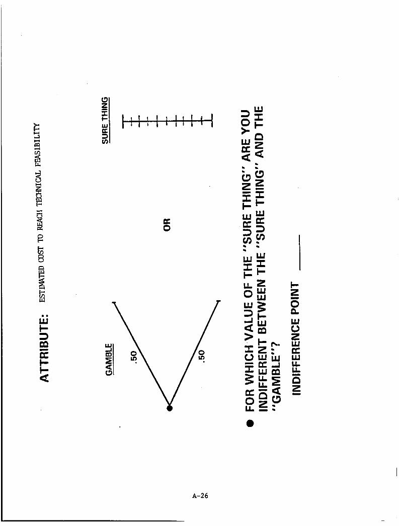
E 8

I- C Q

ct 0

- w E U I

A-26

a .

W

a

0 rl

3 rl m

a 0

m

W I c P z a b f z c W ec 3 cn W I t 2 W

-

: c w

I- 2 w U W LL LL

m

E z -

-. v) W I- < I- v)

c cn U s U i3 I I-

I-

w U

a

: cn W c 3 P

c c E

a a w I I- O mJ

2 k I c s W 2 x 3 0 * u, -

-* cn W I- c cn t m W

pc W I c

a

m -

A-27

a 0

L 0 W 2

I 0 - 5 K 0 LL

3r W u z c w m c z w U w LL LL

W 0

A-28

t 2

e W 0 2 W U W L L

5

- P I 0

A-29

w ii 2 3

m m

W + 3

U c m - c

N

E 0

N

CI-

. w w T X CI-

I- a w w a s cn w I- 3

E: c- c

m - a

L c - a 2 I I-*

A kc- e

I- 2 0 e W 0 z W EL W LL U

-

Ei 2 I

A-30

I- 2

e W 0 2 W U W LL LL

zs

Ei 7 -

A-32

M Q)

t l f I t I l l I ' 1 ' 1 ' 4 ' 1 '

c= 0

M

- - a

c z e W 0 z W U W U u,

5

E 2 -

I- 3

c c

m z a w I 6

e

I- z 0 e W 0 z W U w u, U

-

is 2 m

w U

5

cc w I I- O

I- z e W 0 2 W Et W U

5

5 z -

A-33

iG f i H

m H u

m a

W t- 3

t- k

I- 2

e W 0 2 W U W LL LL

25

Ei 2 w

A-34

a 0

A-35

n c4 . ..r4

n

00 M

0 * PJ

0 rl

In

d r-l r(

0 e N

00

M

0 4

N

Q) 0 rl

A-36

00 b

0 .

L.

0.

t M c= :

A-37

LL

. t 5 t c

. . w X c L Y

E c

U 0

1

00

-

P

s

M

N

Ln

8 d N c4

00

M

N

N E 00 0 rl

M

.. Ly

..

A-39

M

N E 00 0 4 - M

- m.

si

is

M

tu

L n

E 0 -3 N w

00

M

N

N E 00 0 4

M

A-40

0 0 0 0 0 0 oacD*N

I I e

a

E d 4 4 4e - 00

t- .

- 00 M

0 4 N

- N

E co 0 4 - M

N

N E b N

- 00

-

N E

Qo 0 4 - M

-

Fd E

e.

..

A-4 1

U 0

2

si

M

N

.. 9 4

r 0 d r\l #

00 M

N

N E 00 0 r(

M

0 .

w u

w 35 c 3: w z L.. iu m c

e

U

L LL 0

Ei F: s

n w LT

A-42

2

53

M

w

L n

E 0 d N fft

00

M

N

N E 00 3 4

U

!I e

P 8

ei

M

A-4 3

0 .

e

APPENDIX B

FLOW CHART OF INFORMATION FLOWS AND MATEUS PROGRAM

USED TO CALCULATE RANKINGS WITH SAMPLE RUNS

B - 1

The MATEUS Computer Program

The Computer Program MATEUS: K u l t i a t r i b u t e Eva lu t ion of U t i l i t i e s was used t o p r o c e s s t h e i n t e r v i e w d a t a and t o d e t e r m i n e o r d i n a l and c a r d i n a l r a n k i n g s o f t h e a l t e r n a t i v e s y s t e m s f o r i n d i v i d u a l and g r o u p p r e f e r e n c e s . MATEUS is p r e s e n t l y w r i t t e n i n Mic roSof t FORTRAN-80, Release 3.4, December 1980, and w i l l r un on any MicroSoft FORTRAN-80 compatible microcomputers ( w i t h 8080, 8085, 280, 8086, and 8088 m i c r o p r o c e s s o r s ) . M i c r o S o f t FORTRAN-80 is e s s e n t i a l l y e q u i v a l e n t t o FORTRAN I V , and w i t h o n l y minor m o d i f i c a t i o n ( p r i n c i p a l l y in t h e READ and WRITE s ta tements ) should r u n on any computer w i t h a FORTRAN processor. (See also Figure B-1.)

MATEUS does t h r e e m a j o r c o m p u t a t i o n s : ( 1 ) It c a l c u l a t e s t h e m u l t i a t t r i b u t e u t i l i t i e s of outcomes based on t h e Keeney M u l t i p l i c a t i v e Model for m u l t i a t t r i b u t e d e c i s i o n ana lys i s , (2) it c a l c u l a t e s u t i l i t i e s and rankings of a l t e r n a t i v e sys tems based on t h e t h e m u l t i a t t r i b u t e u t i l i t ies of outcomes and a d i s c r e t e p r o b a b i l i t y t ree , and ( 3 ) i t c a l c u l a t e s g r o u p p r e f e r e n c e s corresponding t o three group dec is ion ru l e s .

MATEUS comprises t e n modules, each module p a r t i t i o n e d i n t o lower- leve l modules. F igure B-2 is a Program Tier Chart f o r MATEUS. The number above t h e upper r i g h t corner of a module g ives the calling module. A number preceded by an "SW above t h e upper l e f t corner of a module i n d i c a t e s t h a t t h e module is a subrou t ine called a t more than one place i n t h e Program. Module S1 is called by Module 1.8 and Module 1.1 1. F i g u r e B-3 is a Top-Level Program F l o w c h a r t f o r MATEUS. The top- leve l flowchart h a s a D b l o o p t h a t p rocesses t h e data for each i n d i v i d u a l . Table B-1 g i v e s t h e p r i n c i p a l v a r i a b l e , array, and a r r a y index d e f i n i t i o n s for MATEUS.

Module WAINw is t h e Main Routine for MATEUS and is t h e c a l l i n g r o u t i n e f o r a l l o t h e r r o u t i n e s . It i n i t i a l i z e s t h e d i m e n s i o n s of a l l a r r ays , and c o n t a i n s t h e s t r u c t u r e of t h e DO-loop t h a t p r o c e s s e s t h e da t a f o r e a c h ind iv idua l .

Module 'I)ATAln is called by t h e M A I N Module. It i n p u t s t h e data f o r t he . p r o b a b i l i t i e s of t h e d e c i s i o n tree and t h e a t t r i b u t e states f o r a l l outcomes.

I n t h e a p p l i c a t i o n of MATEUS t o t h e e v a l u a t i o n and r a n k i n g o f E l e c t r i c and Hybr id Vehicles, no p r o b a b i l i s t i c a n a l y s i s was u n d e r t a k e n , so t h a t a l l p r o b a b i l i t y nodes had o n l y o n e path e m a n a t i n g from them, each w i t h a n associated p r o b a b i l i t y of 1 .O.

Module 'I)ATMn is called by t h e M A I N Module. It i n p u t s t h e data f o r t h e c a l c u l a t i o n s f o r e a c h i n d i v i d u a l . The data comprises t h e a t t r i b u t e s c a l i n g c o n s t a n t s and (x ,y) p a i r s of data p o i n t s f o r p i e c e - w i s e l i n e a r f i t s t o t h e a t t r i b u t e u t i l i t y funct ions. I n t h e a p p l i c a t i o n of MATEUS t o t h e eva lua t ion and ranking o f Electric and Hybrid Vehicles, both three-poin t and f ive-poin t fits t o t h e a t t r i b u t e u t i l i t y func t ions were used.

B-3

INTE RV I Ev S

DATA CODING FORMS

CALUC

I)

DECLARES ARRAY SIZES, CALLS ALL SUBROUTINES

PROB

READS ATTRIBUTE DATA, UTILITY FUNCTION PARAMETERS, PERFORMANCE AND WORKLOAD PROBABILITIES

OUTPUT

CALCULATES MASTER SCALING OONSTANT OF MULTIATTRIBUTE UTILITY FUNCTIONS

CONCRD COWUTES GROUP

CALCULATES UTILITIES OF EACH ATTRIBUTL FOR EACH PERFORMANCE-VORKmAD SCENARIO AND FOR EACH INDIVIDUAL

c A

QNIBINES ATTRIBUTE UTILITIES INTO OUTCOME UTILITIES FOR EACH PERFORMANCE- WORKLOAD SCENARIO AND EACH INDIVIDUAL

CONCORDANCE MEASURE

IUNIPUIATES PROBABILITIES ASSIGNED TO PERFORMANCE WHEN PERFORMING SENSITIVITY ANALYSIS (FRACTIONAL FACTORIAL DESIGN)

COMBINES OUTCOME UTILITlES, USING PERFORMANCE AND WORKLOAD PROBMILITICS, INTO SYSTEM UTILITIES FOR EACH INDIVIDUAL, ASSIGNS INDIVIDUAL RANKS TO SYSTEMS

COMPUTES CROUP RANKS USING DECISION RULES

WRITES OUTPUT

Figure B-1. Information Flows and Relevant Computer Programs Used to Rank Alternatives

TIER 1

u DATA 1

u DATA 2

-r----"l -a CALUAT a CALUO

€3 OUTPUT

u CONCRD

TIER 2

F i g u r e B-2. MATEUS P r o g r a m T i e r Chart

B-5

I

I INITIALIZE

I DATA 1 I I 1

CALUAT

E 3 CALUO

+ t

$.

I

I

GROUP 1

1

CONCRD ( GROUP

OUTPUT

+ (-)

F i g u r e B-3. MATEUS T o p - L e v e l P r o g r a m F l o w c h a r t

The MATEUS Computer Program

Module nCALXKM" is called by the M A I N module. It c a l c u l a t e s t h e master s c a l i n g c o n s t a n t f o r t h e K e e n e y M u l t i p l i c a t i v e F o r m u l a t i o n of t h e m u l t i a t t r i b u t e d e c i s i o n a n a l y s i s model, g iven t h e a t t r i b u t e scaling c o n s t a n t s of a n i n d i v i d u a l . It has been proven by Keeney t h a t t h e master s c a l i n g c o n s t a n t mus t be g r e a t e r t h a n -1.0, and t h a t f o r t h e sum of t h e s c a l i n g c o n s t a n t s less than 1.0, t he master sca l ing cons t an t must be greater than 0.0, f o r t h e sum o f t h e s c a l i n g c o n s t a n t s e q u a l t o o n e t h e M u l t i p l i c a t i v e Formulat ion is replaced by a Linear Formulation, and t h a t f o r the sum of t h e scaling c o n s t a n t s greater than 1.0, t h e master s c a l i n g c o n s t a n t must be less t h a n 0.0. T h i s i n f o r m a t i o n is used t o d e t e r m i n e a s t a r t i n g p o i n t f o r a Newton-Raphson i t e r a t i o n f o r t he master scaling constant .

E.

Module CALUAT is called by t h e M A I N Module. It c a l c u l h t e s t h e a t t r i b u t e u t i l i t y f u n c t i o n va lues f o r t h e a t t r i b u t e s of each outcome g iven t h e outcome states and t h e i n d i v i d u a l u t i l i t y functions. .

F. - Module CALUO is c a l l e d by t h e M A I N Module. It c a l c u l a t e s t h e outcome

u t i l i t y f u n c t i o n va lues f o r an i nd iv idua l f o r t h e outcomes, g iven t h e outcone a t t r i b u t e u t i l i t y f u n c t i o n v a l u e s , and t h e i n d i v i d u a l master and a t t r i b u t e scal ing cons tan ts .

Module CALUS is called by t h e M A I N Module. It c a l c u l a t e s t h e a l t e r n a t i v e (system) u t i l i t y f u n c t i o n va lue f o r each a l t e r n a t i v e g iven t h e outcome u t i l i t y f u n c t i o n v a l u e s and t h e p r o b a b i l i t i e s of t h e d e c i s i o n tree. I n t h e a p p l i c a t i o n of MATEUS t o t h e e v a l u a t i o n and r a n k i n g of E l e c t r i c and Hybr id Vehicles, t h e a n a l y s i s was d e t e r m i n i s t i c and the dec i s ion tree de fau l t ed t o p r o b a b i l i t y nodes w i t h one path emanating w i t h p r o b a b i l i t y 1.0.

Module GROUP is ca l l ed by t h e M A I N Module. It c a l c u l a t e s t h e g r o u p d e c i s i o n r u l e v a l u e s f o r three g r o u p d e c i s i o n r u l e s : ( 1 ) The A d d i t i v e Rule , (2) t he Nash Bargaining Rule, and (3) t he Rank Sum Rule.

Module CONCRD is called twice by t h e M A I N Module-once for t h e i n d i v i d u a l rankings and once for the three group d e c i s i o n ru les . It c a l c u l a t e s Kendall 's C o e f f i c i e n t of Concordance.

F i l e ARRAYOFOR is nINCLUDEnd a t c o m p i l e time f o r t h e M A I N Rout ine. It a l loca tes memory space f o r a l l arrays w i t h FORTRAN w D I M E N S I O l w A N D "DOUBLE

B- 7

The MATEXJS Computer Program

PRECISION" statements. the maximum s ize of arrays.

It is t h e only f i l e that has to be modified to change

B-8

I A I C

I D I G I P IS na

J R U N I D

J D I A G

N I A N I C NID N I P NIS

AT( IS, IP, IA)

C H I S Q R ( 1 W ) IRS( 11, IS) I R G ( I G , IS) JDF(1W) PROB ( IS, I P 1 RG ( I G , IS

RS( 11, IS) UAT( IS,IP, IA)

UATC ( I A , I C )

U A T D O A , ID)

US(I1,IS) V G ( I G , I S ) XK( I f , I A ) X K M ( I 1 )

Index f o r A t t r ibu te s . Index U t i l i t y Data. I C = 1 ,.. . , N I C . Index f o r A t t r i b u t e U t i l i t y Data. ID = l , . . . ,NID. Index f o r Group Decision Rules. I G = 1,...,3. Index f o r P r o b a b i l i t y Node Paths. I P = l,...,NIP. Index f o r Systems o r Al te rna t ives . IS = l,...,NIS. Index f o r Kendal l ' s Coe f f i c i en t o f Concordance Group. I W =1,2

I A = l , . . . , N I A . f o r Coeff ic ien ts o f piece-wise l i n e a r f i t t o A t t r i b u t e

I n t e g e r I d e n t i f i e r for t h e Input and Output Data of t h e MATEUS run. Integer Level of Diagnost ic d i s p l a y du r ing run. ( Mot implemented i n Version 1.1.)

Number of A t t r i b u t e s . Number of Coef f i c i en t s . N I C = NID - 2. Number of A t t r i b u t e Data Values. Number o f P r o b a b i l i t y Paths. Number of Systems o r Al te rna t ives .

A t t r i b u t e S t a t e f o r A t t r i b u t e I A of t h e Outccme of P r o b a b i l i t y Path I P for System IS. CHI-Square S ta t i s t ic f o r Group I W . Array RS(I1,IS) converted from real t o i n t e g e r datz type. Array RG(I1,IS) converted from real t o i n t e g e r data type . Degrees of Freedom f o r Group I W . P r o b a b i l i t y ass igned to P r o b a b i l i t y Pa th I P f o r System IS. Preference Rank assigned t o System IS by Group Decis ion Rule I G . Preference Rank assigned t o System IS by Ind iv idua l 11. U t i l i t y ass igned t o Attrdbute I A f o r Outcome o f P r o b a b i l i t y Path I P (by sone Indiv idua l 11). U t i l i t y Coeff icent I C of piece-wise l i n e a r f i t t o U t i l i t y of A t t r i b u t e I A ( f o r some I n d i v i d u a l 11). U t i l i t y Data I D f o r A t t r i b u t e I A (assessed by some I n d i v i d u a l 11). U t i l i t y ass igned t o Outcome o f P r o b a b i l i t y Path I P f o r System IS by I n d i v i d u a l 11. U t i l i t y ass igned to System IS by Ind iv idua l 11. Value ass igned t o System IS by Group Decis ion Rule I C . Scaling Constant assigned t o A t t r i b u t e I A by Ind iv idua l 11. Master Scaling Constant for Ind iv idua l 11.

Table B-1. P r i n c i p a l Variable, Array, and Array Index D e f i n i t i o n s f o r HATEUS.

B-9

File: B:MAIN.FOR

~.+4*..*..tt*+*+.t***+4+4+*++****+*4*ff4+4+++++4**ff**+**+++*+*******+*~

C PROGRAM MATEUS C C THIS IS THE PROGRAM MATEUS: MULTIATT'RIBUTE EVALUATION OF UTILITIES. C I T IS WRITTEN I N MICROSOFT FORTRAN-80, RELEASE 3.4, DECEMBER 1980. C I N GENERAL, FORTRAN PROCESSORS WILL REQUIRE THAT MINOR MODIFICATIONS C BE W E TO THE PROGRAM. C C PROGRAMMER: R. F. MILES, J R . C JET PROPULSION LABORATORY C PASADENA, CALIFORNIA 91009 C C VERSION: 1 . lx l 7/21/83. ~*+..****+tt4t*4.+**4++44+ff*+4*+*4**++4*+*+4+*4*?**4+ff*++4*4*4*44****~

C THIS IS THE M A I N ROUTINE OF THE PROGRAM MATEUS. ~.4***4..*+tt+.+.*ffff*+4a++*++4+*++*+*+***ff*******t***4*ff+*++**+*ff++++~

C THIS IS THE M A I N ROUTINE. I T DECLARES THE SIZES OF THE ARRAYS. I T C IS THE M A I N CALLING ROUTINE FOR ALL SUBROUTINES. I T CONTAINS THE DO C LOOP FOR INDIVIDUALS, I1 = l , . . . , N I I . I T E??DS THE PROGRAM. c-----------------------------------------------------o-------------- C C***C DIMENSION THE ARRAYS.

c--------------------------------------------------------------o-----c C***C INITIALIZATION. {MODULE 21 C

1 0 0 FORMAT ( ' START M A I N ROUTINE' C

110 FORMAT ( / / lX ,7110) C

c--------------------------------------------------------------------c C***C WRITE TITLE TO TERMINAL AND DISK. C C TERMINAL (JUNIT = 5 ) AND D I S K (JUNIT = 8 FOR FILE FORT08.DAT). C

C INSERT "20H" FOR PRINTER AND "OAH" FOR FILE.

{MODULE 1 ) INCLUDE B: ARRAY .FOR

WRITE ( 5 , 1 0 0

READ ( 7 , 1 1 0 ) JRUNID,JDIAG,NII,NIS,NIP,NIA,NID

N I C = N I D - 2

{MODULE 31

DO 150 IU=1,2

I F (IU .€Q. 1 ) LF t 2'20' I F (IU .EQ. 1 ) JUNIT t 5 I F (IU .EQ. 2) LF = Z'OA' I F (IU .EQ. 2) JUNIT = 8

C C *** PROGRAM TITLE ***

WRITE (JUNIT, 120) 120 FORMAT (1X,35X, 'MATEUS')

WRITE (JUNIT,130) LF,LF 130 FORMAT ( A l , 2 O X , 'MULTIATTRIBUTE €VALUATION OF UTILITIES' /Al) C C *** PROGRAM INITIALIZATION PARAMETERS ***

WRITE (JUNIT, 1 4 0 LF, LF, J R U N I D , LF, J D I A G , LF, N I I , LF, NIS, LF, NIP, 1 LF,NIA,LF,NID,LF

140 FORMAT ( A l / A l , 'RUN IDENTIFICATION NUMBER: ',15,/ 1 A1,'DIAGNOSTIC DISPLAY LEVEL: ' ,151

File: B:MAIN.FOR - .

2 A1 , "UMBER OF INDIVIDUALS: ' ,151 3 A1 ,"UMBER OF SYSTEMS: ' ,151 5 AI , "UMBER OF ATTRIBUTES: ' ,151 4 A1 , "UMBER OF PROBABILITY PATHS: *,I51

6 A1 , "UMBER OF ATTRIBUTE DATA: ' , 151A1) 150 CONTINUE C C @++ DELAY TO READ TERMINAL a+*

DELAY = DELAY + 1 .O DO 160 I=l,5000

160 CONTINUE ~ ~ . . ~ . ~ ~ ~ ~ ~ ~ ~ ~ ~ ~ ~ o - ~ ~ - ~ ~ - ~ . o . . ~ ~ ~ ~ ~ ~ ~ ~ ~ ~ ~ ~ - ~ ~ o ~ ~ - ~ ~ o ~ ~ ~ ~ ~ ~ ~ ~ ~ . ~ ~ . . ~ o ~ ~

C+++C INPUT DATA FOR PROBABILITIES AND ATTRIBUTE STATES. C

CALL DATA1 (PROB,AT,NIS,NIP,NIA) c---------------------o------------------o-o-------------------------c C+++C DO LOOP FOR INDIVIDUAL CALCULATIONS. C

{MODULE 4)

{MODULE 5)

DO 180 II=1 ,NII WRITE (5,170) I1

170 FORMAT (/lX,'CALCULATIONS FOR INDIVIDUAL ',I31 c--------------------------.--o--------------------------------------c C@**C INPUT DATA FOR SCALING CONSTANTS AND ATTRIBUTE UTILITY C+++C FUNCTIONS FOR INDIVIDUAL 11. {MODULE 61 C

c-----------------------------------------------o-------------------- C C+*+C CALL SUBROUTINES FOR INDIVIDUAL I1 CALCULATIONS. {MODULE 7) C

CALL DATA2(XK,UATD,II,NII,NIA,NID)

CALL CALXKM(XK,XKM,II,NII,NIA) CALL CALUAT(AT,UATD,UATC,UAT,II,NIS,NIP,NIA,NID,NIC) CALL CALUO(XK,XKM,UAT,UO,II,NII,NIS,NIP,NIA) CALL CALUS(PROB,UO,US,RS,IRS,II,NII,NIS,NIP) c----.----------------------.-----------------------------o----------c

C+++C END DO LOOP FOR INDIVIDUAL CALCULATIONS. {MODULE 5) C 180 CONTINUE c-----------------------------o--.-------o------------.-------------oc C+++C CALCULATE INDIVIDUAL CONCORDANCE. C

c------------------------------o---.----------------------o--------.-c C+++C END CALCULATIONS FOR INDIVIDUALS. C

200 ~ . ~ ~ o . ~ ~ ~ ~ ~ ~ o ~ ~ o ~ ~ o ~ ~ ~ ~ ~ ~ ~ ~ ~ ~ ~ ~ ~ ~ ~ ~ ~ ~ ~ ~ ~ ~ ~ - - - - - - - - - - - - - - ~ ~ - - - - - - - - ~ - ~ ~

C++@C CALCULATIONS FOR GROUP RULES. C

~ ~ . ~ ~ ~ o ~ ~ ~ ~ ~ ~ ~ ~ ~ ~ ~ ~ ~ ~ ~ ~ ~ ~ ~ ~ ~ o ~ ~ ~ ~ ~ ~ . ~ - - - - - - - - - - - - - - - - - - - - - o o - - - ~ o o - . . ~

C@++C CALCULATE GROUP CONCORDANCE. C

1 MODULE 8)

CALL CONCRD(RS,SRX,TIES,STIES,W,CHISQR,JDF, 1 ,NII,NIS)

{MODULE 9 )

WRITE (5,200) FORMAT (/lX,tEND CALCULATIONS FOR INDIVIDUALS'/)

{MODULE 10)

CALL GROUP( US, AS, IRS,VG, RG IRG, NII, NISI

{MODULE 1 1 )

File: B:MAIN.FOR

Fi le : B:DATAl .FOR ~ ~~ ~ ~~~~~

~..4***+i*.i.**.....***+****++++*++++*****+*~******++*++*4*4**+*+44*+~

C SUBROUTINE DATAl 9/5/82 ~.*.4+**...*.+*+..+.++?*?*+****+*++++ff****+ff*+*+4******ff*ff~+++*+*+4ff*~

C SUBROUTTNE DATA1 INPUTS THE DATA FOR PROBABILITIES AND ATTRIBUTE C STATES. ~*..4*+*.*.*..***.***+***?+*+**+*44++**+4*++*+*44*++*++**~***+**++4+*~

SUBROUTINE DATAl(PROB,AT,NIS,NIP,NIA) CI*++4i.+++*4+4ffff**+*9******4**4*+*++*******+*+*0ff*ff+****4*+*4**+**4+C

c***C INITIALIZE. {MODULE 11 C

DIMENSION PROB(NIS,NIP) ,AT(NIS,NIP,NIA) WRITE ( 5 , 1 0 0 )

100 FORMAT ( / ' ENTER SUBROUTINE DATAl 1)

~ ~ ~ ~ ~ ~ ~ ~ ~ ~ ~ ~ o ~ ~ - o ~ ~ ~ ~ ~ ~ ~ - - - - ~ - - ~ ~ ~ ~ ~ o ~ . ~ ~ ~ ~ ~ ~ ~ ~ ~ ~ ~ ~ ~ ~ . o ~ ~ ~ ~ . ~ ~ ~ ~ ~ . . ~ ~ ~

C***C READ & WRITE PROBABILITY DATA PROB(NIS,NIP). {MODULE 21 C

DO 150 IS=l,NIS READ ( 7 , 1 1 0 )

READ (7,120) (PROB( IS, I P ) , I P = l , N I P ) FORMAT ( 1 X , 1 OF7.4 WRITE ( 5 , 1 3 0 ) IS FORMAT ( / l X , 'PROBABILITY DATA FOR OUTCOMES ( I S , I P ) OF SYSTEM',

WRITE ( 5 , 1 4 0 ) (PROB(IS ,XP) , IP= l ,NIP) FORMAT ( l X , 1 OF7.4

110 FORMAT ( 1 x 1

120

130 1 ' ( I S = ' , 1 3 , ' ) ' )

1 4 0 150 CONTINUE c.--------o-------------------------o------------------------o-------c C***C READ & WRITE ATTRIBUTE DATA A T ( I S , I P , I A ) FOR OUTCOMES ( I S , I P ) . C {MODULE 31 C

DO 200 IS=1 ,NIS DO 200 I P = 1 ,NIP

READ ( 7 , 1 6 0 )

READ ( 7 , 1 7 0 ) ( A T ( I S , I P , I A ) , I A = 1 ,NIA) FORMAT ( 5 ( l X , El 4 .4) WRITE ( 5 , 1 8 0 ) I S , I P FORMAT ( 1 X , 'ATTRIBUTE DATA FOR OUTCOME ' , WRITE ( 5 , 1 9 0 ) ( A T ( I S , I P , I A ) , I A = l ,NIA) FORMAT ( 5( 1 X , 1 PE14.4

160 FORMAT (1x1

170

1 80 1 ' ( I S = ' ,13, ' , I P = ' , 1 3 , ' ) ' )

190 200 CONTINUE ~ ~ . ~ ~ ~ ~ ~ ~ ~ ~ ~ ~ o ~ ~ ~ ~ ~ ~ ~ ~ ~ ~ ~ ~ . o ~ ~ ~ ~ . o ~ ~ ~ - ~ - - . - ~ ~ - ~ - ~ - - - - . o - - . - - - - - - - - . ~ ~ ~

C***C EXIT SUBROUTINE DATAl. {MODULE 41 C

999 FORMAT ( ' EXIT SUBROUTINE DATAl '1 C

C

~ + * * 4 * + ~ * * * + + + + * * * * + 4 f f * * f f * * * + + + + * * + + f f * * * * * 4 4 * * * + * ? * * * + + * * ~ * 4 + + * + * 4 + + * ~

WRITE ( 5 , 9 9 9 )

RETURN

END

B-13

Fi l e : B:DATM.FOR

~~*~~*~~~~~*t**.+~~~***************t*************************t*******~

C S U B R O U T I N E D A T A 2 8/28/ 82 ~***********t***+****************************+******t******+*********~

C S U B R O U T I N E D A T A 2 I N P U T S THE DATA F O R THE C A L C U L A T I O N S F O R EACH C I N D I V I D U A L 11. C******t****t******.**********************************************+**~

. . . . . . . . . . . . . . . . . . . . . . . . . . . . . . . . . . . . . . . . . . . . . . . . . . . . . . . . . . . . . . . . . . . . . . S U B R O U T I N E DATA2(XK,UATD,II,NII,NIA,NID)

C*+*C I N I T I A L I Z E . {MODULE 11 D I M E N S I O N XK ( N I I , N I A ) , UATD ( N I A , N I D W R I T E (5,100)

100 FORMAT ( / * E N T E R S U B R O U T I N E D A T U ' ) co---~--.o-*-.. --..--- o~~~~~...~~~~.~~oo~.~~~~~..~....~~o~.~-..~..~.~

C***C READ DATA F O R I N D I V I D U A L (11) {MODULE 2) C

105 FORMAT ( / l X ) READ (7,110) ( X K ( I I , I A ) , I A = l , N I A )

110 FORMAT ( l X , l O F 7 . 4 ) W R I T E (5,120) ( X K ( I 1 , I A ) , I A = l , N I A )

120 FORMAT ( l X , ' S C A L I N G CONSTANTS X K ( I 1 , I A ) '

C READ A T T R I B U T E U T I L I T Y DATA U A T D ( I A , I D ) F O R I N D I V I D U A L (11).

130 FORMAT (1x1

140

READ S C A L I N G C O N S T A N T S XK( 11, I A ) READ (7,105)

1 / ( l X , 1 O F 7 . 4 1 1

READ (7,130)

W R I T E (5,140) FORMAT ( l X , ' A T T R I B U T E U T I L I T Y DATA U A T D ( I A , I D ) ' ) D O 180 I A = 1 , N I A

READ (7,145) 145 FORMAT ( 1x1

READ (7,150) ( U A T D ( I A , I D ) ,ID=l , N I D I 150 FORMAT ( 3( 1 X , El 6.4, F7.4 1

W R I T E (5,160) I A 160 FORMAT ( 1 X , ' A T T R I B U T E ' , I3 )

W R I T E (5,170) ( U A T D ( I A , I D ) ,ID=1 , N I D I 170 FORMAT ( 3( 1 X , 1 PE16.4 , O P F 7 . 4 1 1 180 C O N T I N U E ~ ~ ~ ~ ~ ~ ~ o ~ ~ . o ~ ~ ~ o ~ - ~ ~ ~ ~ ~ ~ ~ ~ ~ ~ ~ . ~ ~ ~ ~ ~ ~ ~ ~ ~ ~ ~ ~ o o ~ ~ ~ ~ ~ - - - o - - - ~ - - - o ~ - - o - - - - ~

C***C E X I T S U B R O U T I N E D A T A 2 . {MODULE 99)

999 FORMAT ( ' E X I T S U B R O U T I N E D A T U ' ) C

C

C*******t***++********************************t***t********t*********~

W R I T E ( 5,999 1

RETURN

E N D

B-14

Fi le : B:CALXKM.FOR

C4+++4++4++++++4+++4++t++++*+4+*++ttt+4++++++++++++4+++++4*+++4*+4+++c

2/6/ 83 C S U B R O U T I N E CALXKM ~4++++.++++++++++++.+**44++++4+4*+t+t+++4+*4+*+++++4+4++44+++++44++++~

C S U B R O U T I N E CALXKM C A L C U L A T E S THE MASTER S C A L I N G CONSTANT X K M ( I 1 ) . C4++++4++++++.+ff+++*4++++4+4+++4+*+te+++++4++++++++++++*++++++++*+4+4~

~*.+++++4+++.++++++++++*+4++44++++4+t++*4++++4++++4*+++4++++*++++++++~ S U B R O U T I N E CALXKM(XK,XKM,II,NII,NIA)

C4.W I N I T I A L I Z E . {MODULE 1 } C

DOUBLE P R E C I S I O N X K M ( N 1 I ) ,FG,G,DG,XKML D I M E N S I O N XK ( N I I , N I A ) W R I T E (5,100)

100 FORMAT ( / ' E N T E R S U B R O U T I N E CALXKM') C C a44 W R I T E S C A L I N G CONSTANTS X K ( N I 1 , N I A ) ++4

1 1 0 W R I T E (5,110) 11 FORMAT ( / 1 X , ' S C A L I N G CONSTANTS XK ( 11, I A ) F O R I N D I V I D U A L ( II= ' , W R I T E (5,120) ( X K ( I 1 , I A ) , I A = l , N I A )

1 13 , ' ) ' )

120 FORMAT ( l X , l O F 7 . 4 )

C4a.C TEST F O R S I G N O F X W i ( I 1 ) . C

c--------------------------------------------------------------------c {MODULE 2)

S X K = 0.0 DO 130 I A = l , N I A

S X K = S X K + X K ( I I , I A ) 130 CONTINUE C

W R I T E (5.140) I I . S X K 140 FORMAT ( l X , ' S U M OF A T T R I B U T E SCALIMG C O N S T A N T S F O R I N D I V I D U A L ',

1 ' (II= ' , I3 , ' ) IS: ' ,F8.4) C

I F ( A B S ( S X K - 1 . 0 ) .LT. 1.OE-3) GO T O 160 I F ( S X K .GT. 1.0) G O T O 150 I F ( S X K .LT. 1.0) GO T O 170

~ ~ ~ ~ ~ ~ ~ o ~ ~ ~ ~ ~ ~ ~ ~ ~ ~ ~ ~ ~ ~ ~ ~ ~ ~ ~ ~ ~ ~ ~ o ~ ~ o ~ ~ o ~ ~ ~ ~ ~ ~ ~ - ~ - - ~ ~ ~ ~ - - ~ ~ - ~ - - ~ o ~ ~ ~ ~ ~ ~ ~

C 4 + 4 C I N I T I A L I Z E X K M ( I 1 ) . {MODULE 31 C C @.4 I N I T I A L XKM < 0 4++ 150 X K M ( I 1 ) = -1.0

C C I N I T I A L XKM = 0 a+* 160 X K M ( I 1 ) = 0.0

C C *a* D E T E R M I N E I N I T I A L XKM > 0. I T E R A T I O N R E Q U I R E D +a+ 170 C O N T I N U E

X K M ( I 1 ) = 1.0 F G = 0.0

180 C O N T I N U E X K M ( I 1 ) = 2 + X K M ( I I ) WRITE (5,185) II,XKM(II) ,FG

G O TO 200

G O TO 230

185 FORMAT ( l X , ' I T E R A T E F O R X K M ( I I : ' , I 3 , ' ) > 0.0. XKM =',F11.8, 1 ' F G = ' , lPE16.8)

B-15

Fi le : B:CALXKM.FOR

C 200 C

21 0

220

225

C O N T I N U E

G = 1.0 D O 210 I A = l , N I A

C O N T I N U E F G = l . O + X K M ( I I ) - G DG = 0.0 D O 220 IA=1 , N I A

C O N T I N U E DG = 1.0-DG XKML = X K M ( I 1 ) XKM( 11) = XKM( 1 1 ) - F G / D G W R I T E (5,225) I I , X K M ( I I ) FORMAT ( lX, 'NEWTON-RAPHSON I T E R A T I O N . X K M ( I I = ' , I 3 , * ) =',F11.8)

G O T O 230

G = G+( 1 . O + X K M ( I I ) * X K ( I I , I A ) )

DG = DG+(XK(II,IA)/(l.O+XKM(II)*XK(II,IA)))+G

I F ( D A B S ( X K M ( I I ) - X K M L ) .GT. 1 . O E - 8 ) G O T O 200

c-----------------------------------------------------------------oo-c C++*C W R I T E X K M ( I 1 ) F O R I N D I V I D U A L (11). {MODULE 51 C 230 C O N T I N U E C

240

~ ~ ~ ~ ~ ~ o ~ ~ ~ ~ ~ ~ ~ ~ ~ ~ ~ ~ ~ ~ ~ ~ ~ ~ ~ ~ ~ ~ ~ ~ ~ ~ ~ ~ ~ ~ ~ ~ ~ ~ ~ . o ~ ~ ~ ~ ~ ~ ~ o ~ ~ ~ ~ ~ - ~ ~ - ~ o o - - . - - ~

C + + W W R I T E X K ( I I , I A ) , S X K , AND X K M ( I 1 ) T O D I S K . {MODULE 61 C

C C +*+ W R I T E A T T R I B U T E S C A L I N G C O N S T A N T S XK( N I I , N I A ) **+ 250 FORMAT ( A l / A l , ' A T T R I B U T E S C A L I N G C O N S T A N T S X K ( I 1 , I A ) F O R ', C

W R I T E (5,240) I I , X K M ( I I ) FORMAT ( l X , ' M A S T E R S C A L I N G CONSTANT F O R I N D I V I D U A L (11=',13,

1 '1 IS: t ,Fl l .8)

LF = Z'OA'

W R I T E (8,250) LF,LF,II

1 'INDIVIDUAL ( II= 9 ,13,* 1 * 1

D O 270 I A H = l , N I A , 1 0 I A N = I A M + 9 I F ( I A N .GE. N I A ) I A N = N I A W R I T E (8,260) LF, ( X K ( I 1 , I A ) , I A = I A M , I A N )

I F ( I A N .EQ. N I A ) G O TO 280 26 0 FORMAT ( A 1 ,10F7.4)

270 C O N T I N U E 280 C O N T I N U E C

B-16

~ ~~

File: B:CALXKM.FOR

C

290 FORMAT (A1 , 'SUM O F A T T R I B U T E SCALING CONSTANTS FOR I N D I V I D U A L ', C C *** W R I T E MASTER SCALING CONSTANT X K ( I 1 ) *** 300

*** W R I T E SUM O F A T T R I B U T E SCALING CONSTANTS SXK *** W R I T E (8,290) L F , I I , S X K

1 (II= ', 13, ' 1 IS: ' , F 8 . 4 )

W R I T E (8,300) L F , I I , X K M ( I I ) FORMAT (A1 , 'MASTER S C A L I N G CONSTANT F O R I N D I V I D U A L (11=c,13,c)c,

1 I S : * , F 1 1 . 8 ) c------------------..--------.-----------.----.----.-----~-------.~--c C***C E X I T SUBROUTINE CALXKM. C

999 FORMAT ( / ' E X I T SUBROUTINE CALXKM') C

C

~*.+*.+.*t*+.+**.*+.+**+ff***+*****+*~tff********ffff***t**+**ff44****+ff**~

{MODULE 7)

W R I T E ( 5 , 999 1

RETURN

END

B-17

F i l e : B : CALUAT. F O R

......................................................................

...................................................................... C S U B R O U T I N E CALUAT 2/7/83

C S U B R O U T I N E CALUAT C A L C U L A T E S T H E A T T R I B U T E U T I L T I m F U N C I O N V A L U E S C U A T ( I S , I P , I A ) F O R T H E A T T R I B U T E S I A O F EACH OUTCOME ( I S , I P ) F O R EACH C I N D I V I D U A L 11. C++++++++++++++++++++++++++++++++++++++++++++++++++++++++++++++++~+++~

...................................................................... S U B R O U T I N E CALUAT(AT,UATD,UATC,UAT,II,NIS,NIP,NIA,ND,NIC)

C+++C I N I T I A L I Z E . {MODULE 11

1 A T ( N I S , N I P , N I A ) , D I M E N S I O N

2 UATD( NIA, NIDI ,UATC( NIA, NIC) ,UAT( NIS, NIP, NIA) W R I T E (5,100)

100 FORMAT ( / ' E N T E R S U B R O U T I N E CALUAT')

C+++C W R I T E A T T R I B U T E U T I L I T Y DATA F O R I N D I V I D U A L (11).

110

c--------------------.--------------o-------------.--------o--------oc {MODULE 2)

W R I T E (5,110) I1 FORMAT ( / l X , ' A T T R I B U T E U T I L I T Y DATA U A T D ( I A , I D ) F O R I N D I V I D U A L ' ,

DO 140 IA=1 , N I A 1 (11=' ,13, ' ) ' )

W R I T E (5,120) I A

W R I T E (5,130) ( U A T D ( I A , I D ) , I D = l , N I D I F O R K A T ( 3( 1 X , 1 PE16.4 , O P F 7 . 4 1 1

120 FORMAT ( l X , ' A T T R I B U T E ',I31

130 140 C O N T I N U E c------------------------------------------.-------------------------c C + + + C CALCULATE A T T R I B U T E U T I L I T Y F U N C T I O N C O E F F I C I E N T S U A T C ( I A , I C ) C F O R I N D I V I D U A L (11). {MODULE 3)

N I C C = N I C - 1 DO 170 IA=l , N I A

DO 170 I C = l , N I C C , 2 A T 1 = U A T D ( I A , I C ) A T 2 = U A T D ( I A , I C + 2 ) U T I L 1 = UATD( I A , I C + 1 ) U T I L 2 = U A T D ( I A , I C + 3 ) I F (AT2 .NE. A T 1 1 GO T O 150 A = 0.0 B = 0.0 GO TO 160

150 C O N T I N U E A = ( U T I L 2 - U T I L l ) / ( A T 2 A T 1 ) B = UTILl - A T l + A

160 C O N T I N U E U A T C ( I A , I C ) = A U A T C ( I A , I C + l ) = B

170 C O N T I N U E

CwclclC W R I T E A T T R I B U T E U T I L I T Y F U N C T I O N C O E F F I C I E N T S U A T C ( I A , I C ) C F O R I N D I V I D U A L (11). {MODULE 4)

180 FORMAT ( / l X , ' A T T R I B U T E U T I L I T Y F U N C T I O N C O E F F I C I E N T S ',

G-----------o------o---------------------------------------ooo------C

W R I T E (5,180) I f

1 'UATC( I A , I C ) F O R I N D I V I D U A L ( 11= ' ,13, ' ' D O 210 I A = l , N I A

W R I T E (5,190) I A

B-18

File: B:CALUAT.FOR

190 FORMAT (lX,'ATTRIBUTE ',I3)

200 FORMAT (5(1X,lPE14.4)) 210 CONTINUE ~ ~ ~ ~ ~ ~ ~ ~ ~ o ~ ~ - ~ ~ ~ . - - - ~ . o - - - - - - - . o - o ~ ~ o o ~ ~ ~ ~ ~ ~ ~ ~ ~ o o ~ ~ . ~ ~ ~ ~ ~ . ~ ~ ~ ~ ~ o ~ o - o . ~

C+++C WRITE ATTRIBUTE DATA AT(IS,IP,IA) FOR OUTCOMES (IS,IP). C {MODULE 5)

220 FORMAT (lX/lX,'ATTRIBUTE DATA AT(IS,IP,IA)')

WRITE (5,200) (UATC(IA,IC),IC=I,NIC)

WRITE ( 5,220)

DO 250 IS=l,NIS DO 250 IP=l ,NIP WRITE (5,230) IS,IP FORMAT ( lX, 'ATTRIBUTE DATA FOR OUTCOIE ' ,

' (IS= ' ,I3, ' , IP= ' ,I3, ' ) ' ) WRITE (5,240) (AT(IS,IP,IA) ,IA=l ,NIA)

230 1

240 FORMAT (5(1X,lPE14.4)) 250 CONTINUE ~ ~ ~ ~ ~ ~ ~ ~ ~ ~ ~ ~ ~ ~ ~ ~ o ~ ~ ~ ~ ~ ~ ~ ~ - - - ~ ~ ~ ~ ~ ~ o ~ ~ ~ ~ ~ ~ ~ ~ ~ ~ ~ ~ ~ ~ ~ ~ ~ ~ o ~ ~ ~ o ~ o ~ o ~ ~ ~ ~ o ~ ~ ~ ~

C+*+C CALCULATE ATTRIBUTE UTILITIES UAT(IS, IP, IA) . {MODULE 6 1 DO 260 IS=1 ,NIS

DO 260 IP=l,NIP DO 260 IA=l ,NIA

DO 258 ID=3,NID,2 IF ((UATD(IA,l) .LT. UATD(IA,3))

1 .AND. (AT(IS,IP,IA) .GT. UATD(IA,ID))) 2 GO TO 258

IF ((UATD(IA,l) .GT. UATD(IA,3)) 1 .AND. (AT(IS,IP,IA) .LT. UATD(IA,ID))) 2 GO TO 258

I C = I D - 2 UAT(IS,IP,IA) = UATC(IA,IC)+AT(IS,IP,IA)

GO TO 260 1 + UATC(IA, IC+1)

258 CONTINUE

260 CONTINUE ~ ~ ~ ~ ~ ~ ~ ~ ~ ~ ~ ~ ~ . ~ o ~ ~ ~ ~ ~ ~ o ~ ~ ~ ~ ~ ~ ~ ~ o ~ o ~ ~ ~ ~ ~ ~ ~ ~ ~ ~ ~ ~ ~ ~ ~ ~ o ~ ~ ~ ~ ~ ~ ~ ~ ~ ~ ~ o o ~ ~ ~ ~ o ~

C*+*C WRITE ATTRIBUTE UTILITIES UAT(IS,IP,IA) FOR ALL OUTCOMES C (IS,IP). {MODULE 7)

265 WRITE (5,265) I1 FORMAT (/lX,'ATTRIBUTE UTILITIES FOR INDIVIDUAL (II=',I3,')') DO 290 IS=1 ,NIS DO 290 IP=1 ,NIP WRITE (5,270) IS,IP FORMAT (lX,'ATTRIBUTE UTILITIES UAT(IS,IP,IA) FOR ',

1 'OUTCOME (IS= ' ,I3, ' , IPn ' ,I3, ' ' WRITE (5,280) (UAT(IS,IP,IA) ,IA=l ,NIA) FORMAT ( lX, 1 OF7.4)

270

280 290 CONTINUE ~ooI~o~~o~o~.o~~~o~...~oooo..~~o~~~~ - ~ ~ ~ o ~ - ~ o . o ~ o - - ~ ~ ~ o . ~ ~ ~ ~ o . ~ ~ o o ~ ~ o ~

Car% EXIT SUBROUTINE CALUAT. {MODULE 99)

999 FORMAT ( / ' EXIT SUBROUTINE CALUAT') C

WRITE (5,999)

RETURN

F i l e : B : CALUAT. FOR

C

...................................................................... END

B-20

File: B:CALUO.FOR

~*+.+ff+.+++*ff*+.++*.?4+**+*+*+4++4ff+ff+*+*++*+44++++++4+4#++++4+*+++ff~

2/6/ 83 C SUBROUTINE CALUO ~++*++++++4*++++4.4++++*+++*+++*+*+*ff+44++++++**++4++++*+ff+ffff+++*4++~

C SUBROUTINE CALUO CALCULATES THE OUTCOME U T I L I T Y FUNCTION VALUE C U O ( I S , I P ) FOR EACH OUTCOME ( I S S I P ) FOR EACH I N D I V I D U A L (11). ~*+**++*+..++*+..*t@+*+*++**+++*4**++t**+++++4++*+*+4+4+*++++44++*#+4~

SUBROUTINE CALUO(XK,XK4,UAT,UO,II,NII, N I S , N I P , N I A ) ~i++t.+.+i++++.*+**.+*+*+++*44+*+*+++++*++++++*++++4+++++**+++44****+~

C**@C I N I T I A L I Z E . {MODULE 1 ) DOUBLE P R E C I S I O N X K M ( N I I ) , PROD DIMENSION XK(NII,NIA),UAT(NIS,NIP,NIA),UO(NIS,NIP) W R I T E (5,100)

100 FORMAT ( / ' m T E R SUBROUTINE CALUO')

C***C W R I T E SUBROUTINE I N P U T ARRAYS.

110

...................................................................... {MODULE 2 )

W R I T E (5,110) I1 FORMAT ( / l X , ' A T T R I B U T E SCALING CONSTANTS FOR I N D I V I D U A L (II=',

W R I T E (5,120) ( X K ( I 1 , I A ) , I A = l , N I A )

W R I T E (5,130) I I , X K M ( I I ) FORMAT ( l X , ' M A S T E R S C A L I N G CONSTANT FOR I N D I V I D U A L ( I I = * , I 3 , ' ) ' ,

W R I T E (5,140) I1 FORMAT ( / l X , * A T T R I B U T E U T I L I T I E S FOR I N D I V I D U A L (11= ' ,13 , ' ) ' ) DO 170 I S = l , N I S

1 13 , ' ) ' )

120 FORMAT ( 1 0 ( 1 X , F 7 . 4 ) )

130 1 IS: * ,F11.8)

140

DO 170 I P = l , N I P W R I T E (5,150) I S , I P

150 FORMAT ( l X , ' A T T R I B U T E U T I L I T I E S U A T ( I S , I P ) FOR ', W R I T E (5,160) (UAT(IS,IP,IA),IA=l,NIA) FORMAT ( 1 X , 1 O F 7 . 4

1 'OUTCOME (IS= ' , I3 , * , IP= * , I3, ' ' 1

160 170 CONTINUE ~ ~ ~ ~ ~ ~ ~ ~ ~ ~ ~ ~ ~ . ~ . . ~ ~ ~ o ~ ~ ~ ~ ~ ~ ~ ~ ~ ~ ~ ~ ~ ~ ~ - ~ o . ~ ~ - o ~ ~ ~ - - - - - . . - - - - - - . - - - - o . - ~ ~

C4*4C TEST FOR A D D I T I V E OR M U L T I P L I C A T I V E U T I L I T Y FUNCTION. C**+C {MODULE 3)

I F ( X K M ( I 1 ) .EQ. 0 . 0 ) GO TO 180 I F ( X K M ( I 1 ) .NE. 0 . 0 ) GO T O 210

c------------..-.---------------------------------------------.--...-c C***C CALCULATE A D D I T I V E U T I L I T I E S U O ( I S , I P ) FOR OUTCOMES (IS, I P ) . C***C {MODULE 4) 180 CONTINUE

DO 200 I S = l , N I S DO 200 IP=1 , N I P

U O ( I S , I P ) = 0.0 DO 1 90 I A r l , N I A

uo( IS, IP) = uo( IS, IP) + XK (11, IA) *UAT( IS, IP, IA) 190 CONTINUE 200 CONTINUE

c- .----~----..--.-------..----..----------------.----.----...--.-..-.c C***C CALCULATE M U L T I P L I C A T I V E U T I L I T I E S U O ( I S , I P ) FOR OUTCOMES C*+*C (IS,IP). {MODULE 51 210 CONTINUE

GO TO 235

DO 230 I S = l , N I S

B-2 1

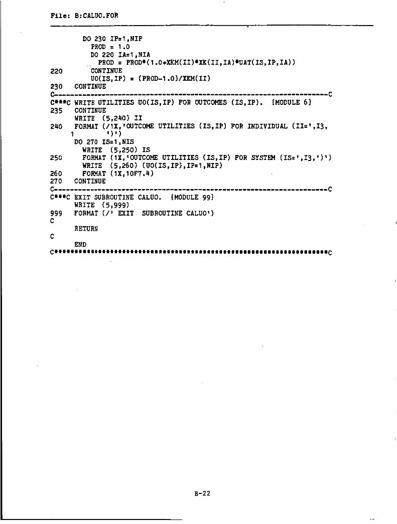
I Fi l e : B:CALUO.FOR

DO 230 IP=I ,NIP PROD = 1.0 DO 220 I A = l , N I A

PROD = PROD+(l.O+XKM(II)~XK(II,IA)*UAT(IS,IP,IA~~ 220 CONTINUE

U O ( I S , I P ) = (PROD-1 . O ) / X K M ( I I ) 230 CONTINUE ~ o o ~ ~ ~ ~ ~ ~ ~ ~ ~ . ~ ~ ~ ~ o ~ ~ ~ ~ ~ - . ~ ~ . ~ ~ o o o . ~ ~ o ~ ~ ~ . ~ o ~ ~ o o ~ ~ . o ~ . ~ . ~ o ~ o ~ . ~ ~ ~ ~ o . ~ ~

C*+4C W R I T E U T I L I T I E S U O ( I S , I P ) FOR OUTCOMES ( IS , IP ) . 235 CONTINUE

240

{MODULE 61

W R I T E (5,240) I1 FORMAT ( / lX ,*OUTCOME U T I L I T I E S ( I S , I P ) FOR I N D I V I D U A L (11=',13,

DO 270 IS=1 , N I S 1 '1 ')

WRITE (5,250) IS FORMAT ( lX , 'OUTCOME U T I L I T I E S ( I S , I P ) FOR S Y S T E N ( IS= ' , I3 , ' ) ' ) WRITE (5,260) ( U O ( I S , I P ) , I P = l , N I P ) FORMAT ( l X , 1 OF7.4

250

26 0 270 CONTINUE ~ ~ ~ ~ ~ ~ ~ ~ ~ ~ ~ ~ ~ ~ ~ ~ ~ ~ ~ ~ - ~ ~ ~ ~ ~ ~ ~ ~ ~ ~ ~ ~ ~ ~ . ~ ~ ~ ~ ~ ~ ~ ~ ~ ~ ~ ~ ~ . o ~ . . o o . ~ . ~ . ~ . ~ ~ ~ o o . ~

C+++C E X I T SUBROUTINE CALUO. {MODULE 99)

999 FORMAT (/I E X I T SUBROUTINE CALUO') C

C

C++++++++++i++++++++~++++++++4+++++++++++++++++++++++++++++++++++++++C

W R I T E ( 5,999 1

RETURN

END

Fi l e : B:CALUS.FOR

~+++++.++.++*++.++.++4++++*++4*++++*+44*+++++?++++++++*++++++++++++++~

C SUBROUTINE CALUS 9/ 8/ 82 ......................................................................

C SUBROUTINE CALUS CALCULATES THE SYSTEl UTILITY FUNCTION VALUE C US(I1,IS) FOR EACH SYSTPl ( IS ) FOR EACH I N D I V I D U A L (11). C++*+++*+++.+++++++++++++~+++++++++++++++++*++++++++++*4+4++4++++++++~

C+++++++++++.++++i++++++++++++++4++++4+++++++++++++++++++++++++*++++4c SUBROUTINE CALUS(PROB,UO,US,RS,IRS,II,NII,NIS,NIP)

C*++C INITIALIZE. {MODULE 1 ) C

DIMENSION 1 PROB(NIS,NIP),UO(NIS,NIP), 2 US ( N I I , NIS , RS( N I I , NIS , I R S( NII , NIS )

WRITE (5,100) FORMAT ( / ' ENTER SUBROUTINE CALUS' ) 100

~ ~ ~ o o ~ ~ ~ ~ ~ o ~ ~ ~ ~ ~ o ~ o ~ ~ ~ ~ ~ ~ ~ ~ o o ~ ~ ~ ~ o ~ ~ ~ ~ ~ ~ o ~ ~ o o ~ ~ ~ ~ ~ ~ ~ o . o o ~ ~ . ~ o ~ ~ o o ~ ~ o ~ ~

C+++C WRITE SUBROUTINE INPUT ARRAYS. C

110

{MODULE 2)

WRITE (5,110) FORMAT (/lX,'PROBABILITIES PROB(IS,IP) FOR OUTCOMES ( I S , I P ) ' ) DO 140 IS=1 ,NIS

WRITE (5,120) IS FORMAT ( 1 X , ' PROBABILITIES PROB( IS , I P

WRITE (5,130) (PROB(IS,IP),IP=l ,NIP)

120 FOR OUTCOMES ( IS, I P ) ' , 1 'FOR SYSTEN ( I S = ' , 1 3 , ' ) ' )

130 FORMAT (lX,lOF7.4) 140 CONTINUE C

150 WRITE (5,150) I1 FORMAT (/lX,'OUTCOME UTILITIES ( IS , IP ) FOR I N D I V I D U A L (11=',13,

DO 180 IS=l ,NIS 1 '1')

WRITE (5,160) I S FORMAT ( 1 X, ' OUTCOME UTILITIES ( IS , I P ) FOR SYSTEM (IS= ' , I3, ' '

FORMAT ( 1 X, 1 OF7.4

160

170 180 CONTINUE

WRITE (5,170) (UO(IS,IP),IP=l,NIP)

- C++*C CALCULATE UTILITIES US(I1,IS) FOR SYSTEMS ( IS ) . {MODULE 3) C

DO 200 IS=1 ,NIS US(I1,IS) = 0.0 DO 190 IP=l ,NIP

US( 11, IS) = US( 11, IS) + PROB( IS, I P ) *UO( IS, IP) 190 CONTINUE 200 CONTINUE ~ ~ ~ ~ o . . ~ ~ o ~ o ~ . o ~ ~ ~ ~ ~ ~ ~ ~ o ~ o ~ ~ ~ ~ ~ ~ ~ o ~ ~ - ~ ~ o ~ ~ ~ ~ ~ ~ o ~ - - - - - - - ~ o - o . o ~ o ~ ~ ~ . . o ~

C*++C WRITE UTILITIES US(I1,IS) FOR SYSTDS ( I S ) FOR I N D I V I D U A L ( I f ) . C*+*C {MODULE 4) C

210

220 FORMAT (lX,lOF7.4) c ~ o ~ o ~ o ~ ~ ~ o ~ ~ o ~ ~ ~ ~ ~ ~ ~ ~ ~ ~ ~ o ~ o o ~ ~ o ~ o ~ - - - - - ~ . - - - - - ~ - ~ ~ - o o - o o ~ ~ ~ ~ ~ o ~ ~ ~ ~ ~ ~ ~

WRITE (5,210) I1 FORMAT (/lX,'UTILITIES US(I1,IS) FOR I N D I V I D U A L ( I I = ' , I 3 , ' ) * ) WRITE (5,220) (US(II,IS),IS=l,NIS)

B-23

File: B:CALUS.FOR

C**+C CALCULATE RANKS RS(I1,IS) OF ALTERNATIVE SYSTEHS ( IS ) . C***C {MODULE 51 C

DO 240 IS=1 ,NIS RS(I1,IS) = 0.5 DO 230 IIS=I ,NIS

I F (US(I1,IS) .EQ. US(I1,IIS)) RS(I1,IS) = RS(I1,IS) + 0.5 I F (US(I1,IS) .LT. US(I1,IIS)) RS(I1,IS) = RS(I1,IS) + 1.0

230 CONTINUE 240 CONTINUE ~------------------.----~-----.-----~~~~~o~..~o~~~~~~~..---.-o-~o-~~~

C***C WRITE RANKS RS(I1,IS) FOR SYSTPiS (IS) FOR I N D I V I D U A L (11). C***C {MODULE 61 C

250 FORMAT (/lX,*SYSTEM RANKS RS(I1,IS) FOR I N D I V I D U A L (11=* ,13 ,* )* )

260 FORMAT (lX,lOF7.4) c---------------------------------o---------------------o---.--------c C*++C CALCULATE INTEGER RANKS IRS(I1,IS) OF ALTERNATIVE SYSTEMS ( IS ) . C***C {MODULE 71 C

WRITE (5,250) I1

WRITE (5,260) (RS(I1,IS) ,IS=l ,NISI

DO 280 IS=l,NIS IRS(I1,IS) = 1 DO 270 IIS=l ,NIS

I F (US(I1,IS) .LT. US(I1,IIS)) IRS(I1,IS) = IRS(I1,IS) + 1 27 0 CONTINUE 280 CONTINUE c-----o---------------------------------------..-.---------o---------c C**+C WRITE INTEGER RANKS IRS(I1,IS) FOR SYSTEMS ( IS) FOR I N D I V I D U A L C***C (11). {MODULE 81 C

WRITE (5,290) I1 290 FORMAT (/lX,'SYSTEM INTECER RANKS IRS(I1,IS) FOR I N D I V I D U A L *,

1 *(II=* ,13,* ) * ) WRITE (5,300) (IRS(I1,IS) ,IS=l ,NISI

300 FORMAT (lX,lOI7) c-------------------.-.-------o----------------.---------------------c C***C EXIT SUBROUTINE CALUS. {MODULE 9 ) C

999 FORMAT ( / * EXIT SUBROUTINE CALUS') C

C

C+****ff+4*+++ff+*++++********++**+**+***ff**~*4*+*+4+*+****ff~***ff***ff**C

WRITE ( 5,999 1

RETURN

END

B-24

~ ~ ~ ~~

Fi l e : B:GROUP.FOR

C WRITE UTILITIES US(11,IS) FOR SYSTEMS ( IS ) FOR INDIVIDUALS (11) . WRITE (5,110)

110 FORMAT (/lX,'SYSTEM UTILITIES US(I1,IS) FOR INDIVIDUALS (11) ' ) DO 140 I I = l , N I I

WRITE (5,120) I1 FORMAT ( l X , 'UTILITIES US( 11, IS) FOR I N D I V I D U A L (II= ' , 13, ' ' WRITE (5,130) (US(I1,IS) ,IS=l ,NIS)

120

130 FORMAT (lX,lOF7.4) 140 CONTINUE C C

150

WRITE SYSTEM RANKS RS(I1,IS) FOR INDIVIDUALS (11). WRITE (5,150) FORMAT (/lX,'SYSTEM RANKS RS(I1,IS) FOR INDIVIDUALS (11) ' ) DO 180 II=l,NII

WRITE (5,160) I1 FORMAT (lX,'SYSTm RANKS RS(I1,IS) FOR I N D I V I D U A L ( I I = ' (13,

WRITE (5,170) (RS(I1,IS) ,IS=1 ,NISI FORMAT ( 1 X , 1 OF7.4)

160 1 '1')

170 180 CONTINUE C C

190

WRITE SYSTEM INTEGER RANKS IRS(I1,IS) FOR INDIVIDUALS (11) . WRITE (5,190) FORMAT ( l X , ' SYSTPl INTEGER RANKS IRS( 11, IS) FOR INDIVIDUALS ' , DO 220 II=l , N I I

1 ' (11) ' )

WRITE (5,200) I1 FORMAT (lX, 'SYSTEM INTEGER RANKS IRS( 11, IS) FOR I N D I V I D U A L ' , WRITE (5,210) (IRS(I1,IS) ,Ibl ,NISI FORMAT ( l X , 1017)

200 1 ' ( I & ' , 13, ' 1 ' )

21 0 220 CONTINUE

C***C CALCULATION FOR ADDITIVE UTILITY RULE (IG = 1) . C

c ~ ~ ~ ~ o ~ ~ ~ ~ - - ~ ~ ~ ~ - - o ~ ~ ~ ~ ~ ~ ~ ~ ~ ~ ~ ~ ~ ~ o ~ o ~ ~ ~ ~ ~ ~ ~ ~ o ~ ~ ~ . ~ ~ o o . ~ ~ ~ ~ ~ ~ o ~ ~ . ~ o o ~ ~ ~ {MODULE 3)

B-25

F i l e : B:GROUP.FOR

C CALCULATE G R O U P V A L U E S VG( 1 ,IS). D O 240 IS=l , N I S

SUM = 0.0 D O 230 II=l , N I I

SUM = SUM + U S ( I 1 , I S ) 230 C O N T I N U E

240 C O N T I N U E C C CALCULATE G R O U P RANKS R G ( 1 , I S ) .

V G ( 1 , I S ) = S U W N I I

DO 260 IS=1 , N I S R G ( 1 , I S ) = 0.5 D O 250 11s =1 , N I S

I F ( A B S ( V G ( 1 ,IS) - V G ( 1 , I IS )> .LE. 0.5E-4) 1 R G ( 1 , I S ) = R G ( 1 , I S ) + 0.5

I F ( A B S ( VG( 1 ,IS) - VG( 1 VIIS) ) .LE. 0.5E-4) G O T O 250 I F ( V G ( 1 , I S ) .LT. V G ( 1 , I I S ) ) R G ( 1 , I S ) = R G ( 1 , I S ) + 1.0

250 C O N T I N U E 260 C O N T I N U E C C CALCULATE G R O U P I N T E G E R RANKS I R G ( 1 , IS) .

DO 280 IS=l , N I S I R G ( 1 , I S ) = 1 D O 270 11s =1 , N I S

I F ( A B S ( V G ( 1 , I S ) - V G ( 1 , I I S ) ) .LE. 0.5E-4) G O T O 270 I F ( V G ( 1 , I S ) .LT. V G ( 1 , I I S ) ) I R G ( 1 , I . S ) = I R G ( 1 , I S ) + 1

270 C O N T I N U E 280 C O N T I N U E c-----------------------o---------------------o---------------------- C C***C CALCULATION F O R NASH B A R G A I N I N G R U L E ( I C = 2) C C

{MODULE 41

CALCULATE G R O U P V A L U E S V G ( 2 , IS) . DO 300 IS=I ,NIS

PROD = 1.0 DO 290 Ik l , N I I

PROD = PRODBUS( I1 , IS) 290 CONTINUE

PROD = A B S ( P R 0 D ) VG( 2 , IS) = PROD**( 1 . O / N I I )

300 C O N T I N U E C C CALCULATE G R O U P RANKS RG( 2, IS) .

D O 320 IS=1 , N I S R G ( 2 , I S ) = 0.5 D O 310 11s = l , N I S

I F ( A B S ( V G ( 2 , I S ) - V G ( 2 , I I S ) )

I F ( A B S ( V G ( 2 , I S ) - V G ( 2 , I I S ) ) .LE. 0.5C4) G O TO 310

.LE. 0.5C4) 1 R G ( 2 , I S ) = R G ( 2 , I S ) + 0.5

I F ( V G ( 2 , I S ) .LT. V G ( 2 , I I S ) ) R G ( 2 , I S ) = R G ( 2 , I S ) + 1.0 31 0 C O N T I N U E 320 C O N T I N U E C C CALCULATE G R O U P I N T E G E R RANKS I R G ( 2, IS) .

D O 340 IS=1 , N I S I R G ( 2 , I S ) I 1

B-26

File : B:GROUP. FOR

DO 330 11s = 1 ,NIS IF (ABS(VG(2,IS) - VG(2,IIS)) .LE. 0.5E-4) GO TO 330 IF (VG(2,IS) .LT. VG(2,IIS)) IRG(2,IS) = IRG(2,IS) + 1

330 CONTINUE 340 CONTINUE

C@@@C CALCULATION FOR RANK SUM RULE (IG = 3). C C

~ ~ o ~ ~ o ~ ~ ~ ~ ~ ~ ~ ~ ~ - - - o ~ - - ~ - ~ - ~ ~ ~ ~ ~ ~ ~ o ~ ~ o ~ ~ ~ ~ ~ ~ ~ ~ ~ o ~ - - ~ o - ~ ~ - o o ~ ~ - ~ ~ ~ o ~ - ~

{MODULE 5)

CALCULATE GROUP VALUES VG( 3, IS) DO 350 IS=l,NIS VG(3,IS) = 0.0 DO 350 II=1 ,NII VG(3,IS) = VG(3,IS) + RS(I1,IS)

350 CONTINUE DO 360 IS=l ,NIS VG(3,IS) = 1.0 - ((VG(3,IS) NII)/(NIS*NII - NIX))

360 CONTINUE C C CALCULATE GROUP RANKS RG( 3 , IS).

DO 380 IS=1 ,NIS RG(3,IS) = 0.5 DO 370 IIS=1 ,NIS IF (ABS(VG(3,IS) - VG(3,IIS)) .LE. 0.5E-4)

IF (ABS(VG(3,IS) - VG(3,IIS)) IF (VG(3,IS)

1 RG(3,IS) = RG(3,IS) + 0.5 .LE. 0.5E4) GO TO 370

.LT. VG(3,IIS)) RG(3,IS) = RG(3,IS) + 1.0 370 CONTINUE 380 CONTINUE C C CALCULATE GROUP INTEGER RANKS IRG( 3 , IS) .

DO 400 IS=l,NIS IRG(3,IS) = 1 DO 390 IIS=l ,NIS IF (ABS(VG(3,IS) - VG(3,IIS)) .LE. 0.5E-4) GO TO 390 IF (VG(3,IS) .LT. VG(3,IIS)) IRG(3,IS) = IRG(3,IS) + 1

3 90 CONTINUE 400 CONTINUE ~ ~ ~ ~ ~ ~ ~ ~ ~ ~ ~ ~ ~ ~ ~ ~ ~ ~ - ~ ~ ~ ~ ~ ~ ~ ~ ~ ~ ~ ~ ~ ~ ~ ~ ~ ~ o o - o - - - - - - o - o ~ - - - - - - - - - - - - - - ~ - ~ - c C*@*C WRITE GROUP CALCULATION RESULTS. C

410 FORMAT (//lX, 'SYSTEM ADDITIVE RULE NASH RULE

(MODULE 7)

WRITE (5,410) 1

9

1 ' RANK SUM RULE'/lX, ' (IS) VALUE RANK IRANK ' p

2 1 VALUE RmK IRANK VALUE RANK IRANK '/ 3 4

9 ~ ~ , ' o o ~ ~ ~ ~ o o ~ ~ ~ ~ ~ ~ ~ ~ ~ ~ ~ ~ ~ o o ~ o - - ~ - - - - - - - - - - - - - - - o = - - - ~ ~ ~

'1 '~-----~~o-~~--o----r

DO 430 IS=1 ,NIS WRITE (5,420) IS,VG(l,IS),RG(l ,IS),IRG(l,IS),VC(2,IS),

FORMAT ( 111, I3 ,3(F10 e 4 ,F7 -4 ,I5) I 1 RG ( 2, IS) IRG ( 2 9 IS I , VG( 3 IS RG ( 3 9 1s) 9 IRG ( 3 , 1s

420 430 CONTINUE

C@@@C EXIT SUBROUTINE GROUP. C

~ o o ~ ~ ~ ~ ~ ~ ~ ~ ~ ~ ~ o ~ ~ o ~ ~ ~ ~ ~ o ~ o ~ o ~ ~ ~ ~ ~ ~ ~ ~ ~ o o - - ~ - - o = - o - - o - - - - - - - - - - - - - - - - ~ ~ c fMODULE 8)

WRITE (5,999)

B-27

F i l e : B : GROUP. FOR

999 FORMAT ( / ' E X I T SUBROUTINE GROUP' 1 C

C RETURN

END ......................................................................

B-28

~

F i l e : B:CONCRD.FOR

~*.*.+...*....+.*+.+*+*****+**ff+ff*++*+****ff+**+**ff+**+4****4**ff+44+*+~

C S U B R O U T I N E CONCRD 7/21 / 83 ~**..*...*.*.44.**.**ff*+ff+ff******+*ff+****+*4++***++?*+***ffff+4*+******~

C S U B R O U T I N E CONCRD C A L C U L A T E S THE CONCORDANCE S T A T I S T I C S F O R C R A N K I N G S B Y I N D I V I D U A L S OR B Y GROUP D E C I S I O N RULES. ~*.**..*.+.*......++*+4+*4*+4*+**+*+*+****ff++**ff*+++*+ff+**+**?ff*fft4*+~

~ * ~ ~ * ~ ~ . * * * ~ * ~ * . ~ ~ ~ ~ ~ t * ~ + * * * ~ ~ ~ ~ ~ f f ~ f f * * * ~ ~ * ~ * ~ ~ f f * * ~ * * * * f f ~ f f * ~ * ~ * * ~ * ~ ~ * * ~

C***C I N I T I A L I Z E . {MODULE 1 ) C

S U B R O U T I N E CONCRD(RX,SRX,TIES,STIES, W, C H I S Q R , JDF, I W , N I I X , N I S )

D I M E N S I O N 1 R X ( N I I X , N I S ) , 2 S R X ( N 1 S ) , T I E S ( N I I X , N I S ) , S T I E S ( N I I X ) , 3 W(2) , C H I S Q R ( 2 ) , J D F ( 2 )

C

100 FORMAT ( / ' E N T E R S U B R O U T I N E CONCRD' C

110 FORMAT ( / l X , ' I W = ' , 1 1 , 5 X , ' N I I X = ' , 1 3 , 5 X t ' N I S = ' ,I31 C

W R I T E (5,100)

W R I T E (5,110) I W , N I I X , N I S

DO 140 II=1 , N I I X W R I T E (5,120) I1

120 FORMAT ( l X , ' R X ( I I , I S ) F O R I1 =' , I31 W R I T E (5,130) ( R X ( I I , I S ) , I S = l , N I S )

130 FORMAT ( 1 X , 5 F 1 0 . 4 ) 140 C O N T I N U E c------------------------------------------------------------------~---c C***C C A L C U L A T E SUMSQR = SUM O F SQUARES. {MODULE 2) C C

145

150 C

155

160 C C

170 C

1 80 C C

*** SUM OF R A N K I N G S BY S Y S T E M (IS) *** DO 145 IS=1 , N I S

S R X ( 1 S ) = 0.0 C O N T I N U E DO 150 I S = l , N I S

D O 150 II=1 , N I I X S R X ( 1 S ) = S R X ( 1 S ) + R X ( I 1 , I S )

C O N T I N U E

W R I T E (5,155) FORMAT ( / 1 X , ' S R X ( 1 S ) '1

FORMAT ( l X , 5 F 1 0 . 4 ) W R I T E (5,160) ( S R X ( 1 S ) ,IS=1 , N I S I

*** MEAN O F SUM O F R A N K I N G S *+* SRXM = 0.0 D O 170 I S = l , N I S

C O N T I N U E SRXM = SRXM + S R X ( I S ) / N I S

W R I T E (5,180) SRXM FORMAT ( / l X , ' SRXM = ' , 3 X , F 1 0 . 4 )

*** SUM OF S Q U A R E S *** SUMSQR = 0.0

B-29

File: B : CONCRD. FOR

DO l?O IS=1 ,NILS SUMSQR = SUMSQR + (SRX(1S) - SRXM)+*2

190 CONTINUE

C

204

206 C

C

C

C

C 21 0

C 220 C

23 0

C

240 250 26 0 C

270

2 80

DO 204 II=1 ,NIIX DO 204 IS =l ,NIS TIES(I1,IS) = 0.0

CONTINUE DO 206 II=l,NIIX

CONTINUE STIES(I1) = 0.0

DO 260 Ik l ,NIIX DO 250 IS=1 ,NIS

DO 220 IIS=1 ,NIS IF (11s .EQ. IS) GO TO 220

IF ((ABS(RX(I1,IIS) RX(I1,IS)) .LE. 0.53-4) 1 .AND. (11s .LT. IS)) GO TO 250

IF (TIES(I1,IS) .GT. 0.0) GO TO 210

IF (ABS(RX(II,IIS) - RX(II,IS)) .LE. 0.5~4) 1 TIES(I1,IS) = 2.0

GO TO 220

CONTINUE IF (ABS(RX(I1,IIS) RX(I1,IS)) .LE. 0.53-4)

1 TIES(I1,IS) = TIES(I1,IS) + 1.0

CONTINUE

WRITE (5,230) II,IS,TIES(II,IS) FORMAT (lX,'II = ',13,5X,'IS = ',13,lOX,

1 'TIES(I1,IS) = ',F10.4)

STIES( 11) = STIES( 11)

WRITE (5,240) II,STIES(II) FORMAT (lX,'II = ',13,5X,'STIES(II) = ',F10.4)

1 + (1.O/l2.O)*(TIES(II,IS)~~3 - TIES(I1,IS)) CONTINUE

CONTINUE

TTIES 0.0 DO 270 Ih1,NIIX TTIES = TTIES + STIES(I1)

CONTINUE WRITE (5,280) TTIES FORMAT (lX,'TTIES = ',F10.5)

B-30

C***C C***C C

C

C

C

290

CALCULATE W ( I W ) = CONCORDANCE, J D F ( I W ) = DEGREES OF FREEDOM, AND C H I S Q R ( I W ) = C H I SQUARE VALUE. {MODULE 4 )

W ( I w ) = SUMSQR/((l.0/12.O)*(NI~X**2)*(NIS**3 - N I S ) - N I I X * T T I E S )

J D F ( I W ) = N I S - 1

C H I S Q R ( I W ) = N I I X * ( N I S - l)*W(IW)

W R I T E (5 ,290) Iw,W(IW) , I W , C H I S Q R ( I W ) , I W , J D F ( I W ) FORMAT ( l X , ' W ( ' , I l ,'I = ',F10.4,10X,~CHISQR(t,11 , ' I = * , F 1 0 . 4 ,

1 l O X , ' J D F ( ' , I l , ' ) = ' , I S )

B-3 1

F i l e : B : OUTPUT. F O R

~*.*C...*..++*+*+ff+.4*+ff**+**4*9*+***++*~*4+**+4+4+4***++ff*++**ff**++*~

C S U B R O U T I N E OU T P U T 9/ 8/ 82 ~*.*..+*.4.++*+**+..+++++*++ff+*4+*+4*+++4+*ff*+44ffff*+++******+***+*ff*4~

C S U E R O U T I N E OUTPUT FORMATS AND O U T P U T S T H E R E S U L T S O F T H E C CALCULATIONS. ~*.*4*.**+.*++*.+*+.+**++***++*+*++4~+4+*4+*+*+4***ff***4**ff*+***44++ff~

~.****..++.*+++*++4.+++++++4+*+++4++4+++**t*+***4ff*++ff+ff**4**4+*4+44*~

C***C I N I T I A L I Z E . {MODULE 11

S U B R O U T I N E O U T P U T ( U S , I R S , V G , IRG,W,CHISQR,JDF,NII,NIS)

D I M E N S I O N 1 2 W ( 2 ) , C H I S Q R ( 2 ) , J D F ( 2 )

U S ( N I I , N I S ) , I R S ( N I I , N I S ) ,VG( 3, N I S I , I R G ( 3 , N I S I , W R I T E (5,100)

100 FORMAT ( / ' E N T E R S U B R O U T I N E O U T P U T ' ) c--------------------------------------.----.-------~-----~-~---------.c C***C D O LOOP F O R O U T P U T U N I T . {MODULE 21

DO 280 I U = 1 , 2 I F ( I U .W. 1 ) LF = 2'20' IF ( I U .EQ. 1 ) J U N I T = 5 I F ( I U .EQ. 2) LF = Z t O A t I F ( I U .EQ. 2 ) J U N I T = 8 W R I T E (5,110) J U N I T

110 FORMAT ( / l X , ' J U N I T = ' , 1 3 / 1 X ) c--------------------------------------------------------------------c C*+*C OUTPUT P R E F E R E N C E P A G E S B Y I N D I V I D U A L S (11). {MODULE 31 C

I S M = 1 I S N = 20 I F ( I S N .GT. N I S ) I S N = N I S I I M = 1 I I N = 5 I F ( I I N .GT. N I I ) I I N = N I I

C C **** P A G E HEADER *** C 120 C O N T I N U E

130 FORMAT (Al/A1,29X,'MULTIATTRIBUTE D E C I S I O N A N A L Y S I S ' / A 1 , 2 7 X , ' R A N K I N G O F A L T E R N A T I V E S Y S T E M S ( IS) ' /

W R I T E ( J U N I T , 1 30) LF, LF, LF, LF

1 2 A 1 , 3 5 X , ' B Y I N D I V I D U A L S (11)')

W R I T E ( J U N I T , 140) LF, LF, (11, I I = I I M , I I N ) 140 FORMAT ( A l / A l ,6X,~IS',5X,'II=',I~,4~8X,'II=',I3~~

W R I T E ( J U N I T , 1 5 0 ) LF 150 FORMAT ( A 1 , 8 X , 5 ( U T I L I T Y RANK' 1 C C **. I N D I V I D U A L P R E F E R E N C E S ( U S AND I R S ) *** C

D O 170 I S = I S M , I S N W R I T E ( J U N I T , 160) LF, LF, IS, ( U S ( 11, IS) , I R S ( 11, IS) , I I = I I M , I I N )

160 FORMAT (Al/A1,5X,13,2X,5(F6.4,2X,I3,3X)) 170 C O N T I N U E C C *** P A G E L O G I C *e4 C

I F ( I I N .EQ. N I I .AND. I S N .a. N I S ) GO TO 190

B-32

-- File: B:OUTPUT.FOR

IF (IIN .EQ. NII) GO TO 180

IIN = IIN+5 IF (IIN .GT. NII) IIN = NII GO TO 120

ISM = ISM +20 ISN = ISN+20 IF (ISN .GT. NISI ISN = NIS IIM = 1 IIN = 5 IF (IIN .GT. NII) IIN = NII GO TO 120

IIM = 11b5

1 80 CONTINUE 8

190 CONTINUE C C C

200

++a CONCORDANCE FOR INDIVIDUALS +++

WRITE (JUNIT,200) LF,LF,W(l),CHISQR(l),JDF(I) FORMAT (Al/Al ,'W = ',F6.4,10X,'CHI SQUARE = ',F10.2,10X,

1 'DF =',I31 ~ ~ ~ o ~ ~ ~ ~ ~ ~ ~ ~ ~ ~ ~ ~ ~ ~ ~ ~ ~ ~ ~ ~ ~ ~ o ~ ~ ~ ~ ~ ~ ~ ~ ~ ~ ~ ~ ~ ~ ~ ~ ~ ~ ~ ~ ~ ~ ~ ~ ~ o ~ ~ ~ o ~ ~ ~ ~ ~ ~ ~ o ~ ~ ~ ~ ~

C+++C C {MODULE 4) C

OUTPUT PREFERENCE PAGES BY GROUP DECISION RULES (IG).

I ISM = 1 ISN = 20 IF (ISN .GT. NISI ISN = NIS

C C a++ PAGE HEADER +++ C 21 0 CONTINUE

220 FORMAT (Al/A1,19X,'MULTIATTRIBUTE DECISION ANALYSIS'/ Al,17X, 'RANKING OF ALTERNATIVE SYSTR4S (IS) '/

WRITE ( JUNIT , 220 LF , LF , LF , LF 1 2 Al,21X, 'BY GROUP DECISION RULES (IG) '1

WRITE (JUNIT,230) LF,LF,LF,LF FORMAT (Al/A1,6X,'IS',7X,'IG = l',lOX,'IG = 2',10X,'IG = 3'/ 23 0

1 Al,14X,'ADDITTVE',lOX,'NASH' ,lOX,'RANK SUM'/ 2 Al,7X,3(6X,'VALUE RANK'))

C C GROUP PREFERENCES (VG AND RG) ++a C

DO 250 IS=ISM,ISN WRITE FORMAT (A1 /Al,6X, I2 , 4X, 3 (F6.4,2X, I2,6X)

(JUNIT,240) LF,LF,IS, (VG(IG,IS) ,IRG(IG,IS) ,IG=1,3) 240 - 250 CONTINUE C C a++ PAGE LOGIC +++ C

IF (ISN .EQ. NISI GO TO 260 ISM = ISM +20 ISN = ISN+20

GO TO 210 I IF (ISN .GT. NISI ISN = NIS

26 0 CONTINUE

I B-33

F i l e : B : OUTPUT. FOR

B-34

File: B:ARRAY.FOR

. . . . . . . . . . . . . . . . . . . . . . . . . . . . . . . . . . . . . . . . . . . . . . . . . . . . . . . . . . . . . . . . . . . . . . C ARRAY. FOR 6/25/83 . . . . . . . . . . . . . . . . . . . . . . . . . . . . . . . . . . . . . . . . . . . . . . . . . . . . . . . . . . . . . . . . . . . . . .

c**********************************************************************c

C THIS ROUTINE IS TO BE "INCLUDED" IX THE MAIN ROUTINE AT COMPILE C TIME. IT DIMENSIONS ALL THE ARRAYS,

C***C FORMAT FOR DIMENSIONING THE ARRAYS. ALL THE ARRAY DIMENSIONS C MUST BE REPLACED WITH NUMBERS. C C WHERE A "/" IS PRESENT, ENTER THE LARGER OF THE TWO VALUES ON C EITHER SIDE. C C DOUBLE PRECISION XKM(NI1) C DIMENSION C 1 PROB(NIS,NIP), AT(NIS,NIP,NAT), C 2 UATD(NAT,NID), UATC(NAT,NlC), UAT(NIS,NIP,NAT), C 3 XK(NII,NAT), C 4 UO(NIS,NIP), US(NII,NIS), RS(NII,NIS), C 5 VG(S,NIS), RG(3,NIS), C 6 IRS(NII,NIS), IRG(3,NIS), C C 8 W(2),CHISQR(2),.JDF(2) c- -_ - - - - - - -- - - .- ------I -- -- - - - - -- - -- - - -- .- - _. .- - - -. -_ - _- - - - ._ - - - - - - - __ _ _ - - - - - - - - c C***C DIMENSION THESE ARRAYS WITH NUMBERS. C

7 HX ( NI I /3, NI S ) , SRX ( NI S ) , TIES (NI T / 3 , N I S ) , STIES ( NI I /3 ) ,

DOUBTJ2 PREC IS ION XKM ( :10 ) DIMENSION

1 PHOB(18,1), AT(18,3,30), 2 UATD(lO,lO), UATC(10,8), UAT(18,1,10), 3 XK(5,10), 4 U0(18,1), US(5,18), RS(5,18), 5 VG(3,18), RG(3,18), 6 IRS(5,18). IRG(3,18), 7 RX(5,18),SRX(18),TIEs(5,38),STIES(5), 8 W(Z),CHISQR(2),JDF(Z)

c********************Y********* ARHAY.FOR ****************************C

8-35

F i l e : B:CASEINP.053

MATEUS RUN PARAMETERS .JHUN ii) .IDJAG XI I NIS NIP NIA NID

53 0 4 16 1 8 10 PROHAH;I,JTY DATA FOR OUTCOMES ( 'IS, IP) OF SYSTEM ( I S = l )

PROBABILITY DATA FOR OUTCOMES (IS,IP) OF SYSTEM (IS=2)


PRORABILITY DATA FOR OUTCOMES (IS, 1 P ) OF SYSTEM (IS-4)

PROBAR11,ITY DATA FOR OUTCOMES (IS, IP) OF SYSTEM (IS=5)

PKOHAHlLIlY UATA FOR OUTCOMES (IS, IP) OF SYSTEM (IS=6)

PROBAHILITY DATA FOR OL'TCOMES (TS,IP) OF SYSTEM (IS=7)

1 .ooo

1 .ooo

1 .ooo

1 , 0 0 0

1 .00G

1 .ooo

1 .000

1 . O O G

1 . O O G

1 .ooo

1 .ooo

1 .000

1.000

I. 000

1 .ooo

1 .000

PH~BABI L I TY DATA FOR OUTCOMES ( IS, I P OF sys'rm ( 1s=8

PROBAHTLITY DATA EOR OUTCOMES (IS, IP) OF SYSTEM (ISl.9)

PROBAB I I, I TY DATA FOR OUTCOMES ( IS , I P ) OF SYSTEM ( IS- 10 )

PKOBABILiTY DATA FOR OL'TCOMES (IS,IP) OF SYSTEM (IS=ll)


PROHABILITY DATA FOR Ol!T(:OMlCS ( i s , I P ) (::: SYSTEM (1S=l:3)

PHOBABILJTY DATA FOR OUTCOMES ( i S , I f ) OF SYSTEM (1S=14)


PKORABILITY DATA FOR OUTCOMES (IS,IP) OF SYSTEM (IS=16)

ATTRJBUTE DATA AT(IS,IP,IA) FOR OUTCOME (IS=l,ZP=I) 7 . O 42 .O 8.0 6.0 193.OE6 7.0 4.0 3.0

7.0 100.0 6.0 7.0 i 9 8 . O E f i 6.0 4.0 3.0

7.0 31.0 7 . O 7.8 124.OE6 7.0 4 . O 3.0

7 . 0 2 7 . 0 4 .0 6.9 i40.0r6 5.0 2 . 0 3.0

7 . 0 G0.C 4.0 6 . 9 114.OE6 6.0 2.0 3.0

7 . O 80.0 9.0 7.2 143.OE6 8.0 5.0 3.0

ATTRIRL'TE DATA AT(lS,IP,IA) FOR OUTCOME (IS=2,IP=1)

ATTRIBUTE DATA AT(IS,IP,IA) FOR OUTCOME (IS=3,1P=i)

ATTRlBLTTE DATA AT(IS,IP,IA) FOR OUTCOME (IS=4,1P=l)

ATTRIBUTE DATA AT(IS,IP,TA) FOR OUTCOME (IS=5,TY=1)

ATTRIBUTE DATA AT(IS,IP,IA) FOR OUTCOME (IS=G,IP=l)

B-36

Pile: B:CASEINP.053

ATTRIBUTE DATA AT(IS,IP,IA) FOR OUTCOME (IS=7,IP=1) 3.0 50 .0 2.0 3.8 5.0 9.0 3 . 0

8.0 42.0 8.0 6.0 8.0 8.0 3 . 0

8.0 100.0 7.0 7.0 7 .0 8.0 3.0

ATTRIBUTE DATA AT(LS,IP,IA) FOR OUTCOME (IS=lO,ZP=l) 8.0 31 .O 8 . 0 7.8 tl . 0 8.0 3.0

ATTRIBL'TE DATA AT(IS,IP,IA) FOR OUTCOME (IS=ll,IP=l) 8.0 27.0 5 . 0 6.9 6.0 4.0 3 . 0

ATTRIBUTE DATA AT(IS,IP,IA) FOR OUTCOMK (IS=12,IP=1) 8.0 45.0 5.0 7.1 7.0 4.0 3 . 0

ATTRIBL'TE DATA AT(IS,IP,IA) FOR OIJTCOME (IS=13,IP=l) 8.0 108.0 5 . 0 :3 . 9 5 . 0 9.0 3.0

ATTRIBUTE DATA A?'( IS, i P , i A ) %OH OUTCOME (IS=14,IP:l) 8.0 67.0 10.0 6.3

ATTRIBUTE DATA AT(IS,IP,IA) FOR OUTCOME (IS=lS,IP=l) 8 . 0 80.0 10.0 7.4

ATTKIHUTE DATA AT( IS, I P , IA) FOR OIJTCOME ( IS=-16, I F 1 ) 6.0 38.0 7.0 7.6 9.0 10.0 3 * 0

ATTRIBUTE DATA AT(IS,TP,TA) FOR OUTCOME (IS=8,1P=I)

ATTRIBUTE DATA AT(lS,IP,IA) FOR OUTCOME (IS=S,IP=l)

10.0 i3.0 3 . 0

10.0 10.0 3.0

SCALING CONSTANTS XK(I1,IA) FOR INTERVlEW 8 3 . i I = i

ATTRIBUTE UTILITY DATA UATD(IA,ID) FOR INTERVIEW %3. I i = l ATTRIBUTE 1

0.670 0.500 0.620 0.700 0.200 0.300 0.450 0.500

3.0 0.00 5 . 5 0.25 6.5 6.8 0 . 7 5 8.0 1.00

ATTRIBIJTE 2 i08.0 0.00 95.0 0.25 85.0 72.5 0.75 27.0 1 . o o

ATTRIBUTE 3 2 . 0 0.00 4.5 0.25 5 . 0 6.5 0.75 10.0 1.00

3 . 8 0.00 4.8 0.25 5 . 5 6.8 0.75 7.8 1 .oo

ATTRIBUTE 4

ATTRIBUTE 5

213.0E6

200.OE6

19O.OEti

l24.OE6

160.OE6

114.OE6

240. 0EO

135.OE6

135.OE6

170.OE6

0.50

0.50

0 . 5 0

0.50

240.0E6 0.00 195.OE6 0.25 1.70.0E6 0 . 5 0 140.0EG 0.75 1 1 4 . O E 6 1.0C

ATTRIBUTE 6 5.0 0 . 0 0 5 . 8 0.25 6.5 0.50 7.3 0.75 10.0 1 .00

B-37

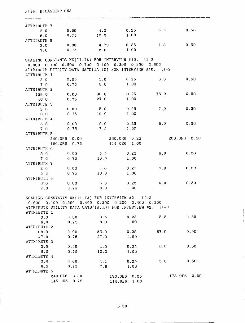
F i l e : B : C A S E I N P . 0 5 3

ATTRIBUTE 7 2 . 0 0 . 0 0 4 .2 0 . 2 5 5 . 5 0 . 5 0 6 . 0 c.75 1 0 . 0 1.00

3.0 0.00 4 .79 0 .25 4 . 8 0.50 7.0 0.75 8 . 0 1.00

ATTRIBUTE 8

SCALING CONSTANTS X K ( I 1 , I A ) FOR INTERVIEW # l o . T1-2

ATTRTBUTE UTILITY DATA l!ATD( I A , 7 1 3 ) FOR TNTERVTEW # l o . IT=2 ATTRIBUTE 1

0 .800 0,100 0.500 0 .700 0.100 0 . 3 0 0 0.200 O.600

3 . 0 G . 00 ,5 . 0 0 . 2 5 6 . 0 7 . 0 0.75 8.0 1 . o c

ATTRIBUTE 2 108.0 0 . 0 0 90.0 0 . 2 5 75.0 40.0 0 .75 27 . O 1.00

ATTHIBIJTE 3 2 * 0 0 .00 5 . 0 0 . 2 5 7 . 0 8 # 0 0 . 7 5 1 0 . 0 1 .00

3 . 8 0 . 0 0 5 . 0 0 .25 6 . 0 7 . 0 0.75 7 . 6 1 I 01:

ATTH I HUTE 4

ATTRIBUTE 5 240.OE6 0 . 0 0 2 3 0 . O E 6 0 . 2r5 200. 180.OE6 0 75 114.OE6 1.00

ATTH 1 BL'TE 6 5 . 0 0 . 00 5 . 5 0.25 6.0 7.0 0.75 10.0 1.00

2.0 0 .00 :: . 0 0 . 2 5 5 . 0 5.0 0.75 10.0 1 .oo

3 . 0 0 . 0 0 5 . 0 0 . 2 5 6 . 0 7 . 0 0.75 8 . 0 1.00

A'PTH T HUTE 7

ATTRIBUl'Z 8

0.50

0 .50

0.50

0 . 5 0

OE6 0 . 5 0

0 .50

0 . 5 0

0 . 5 0

SCALING COXSTANTS X K ( i I , I A ) FOR !ST;:HViIiW % 2 . 11--3

ATTRIBUTE UTILITY IjA'I'A UATl)( I A , 11)) FOR 1N'TF:NV;EW #2. 11-3 ATTRIBUTE 1

0 . 6 0 0 0 . 1 0 0 0.500 0.400 0 .200 0.200 0.400 0 .300

3.0 0.00 3 . 5 0 . 2 5 5.5 0.50 6 . 0 0.75 8.0 1.00

ATTHIBL'TE 2 i 0 8 . 0 0 . 0 0 8 5 . 0 0 . 2 5 67.0 0.50 4 7 . 0 0.75 27 . O 1 .oo

ATTRIBUTE 3 2 . 0 0 .00 4 . 0 0 . 2 5 6 . 0 0 .50 8 . 0 0.75 10.0 1 .00

3 . 8 0 . 0 0 4 . 4 0 . 2 5 5.0 0 . 5 0 6 . 5 0.75 7 . 8 1 . o o

ATTRIBUTE 4

ATTRIBUTE 5 240.0E6 0 . 0 0 1 9 0 . O E 6 0 . 2 5 175.OE6 0 . 5 0 145.0&6 0 . 7 5 114.OE6 1.00

E 3 8

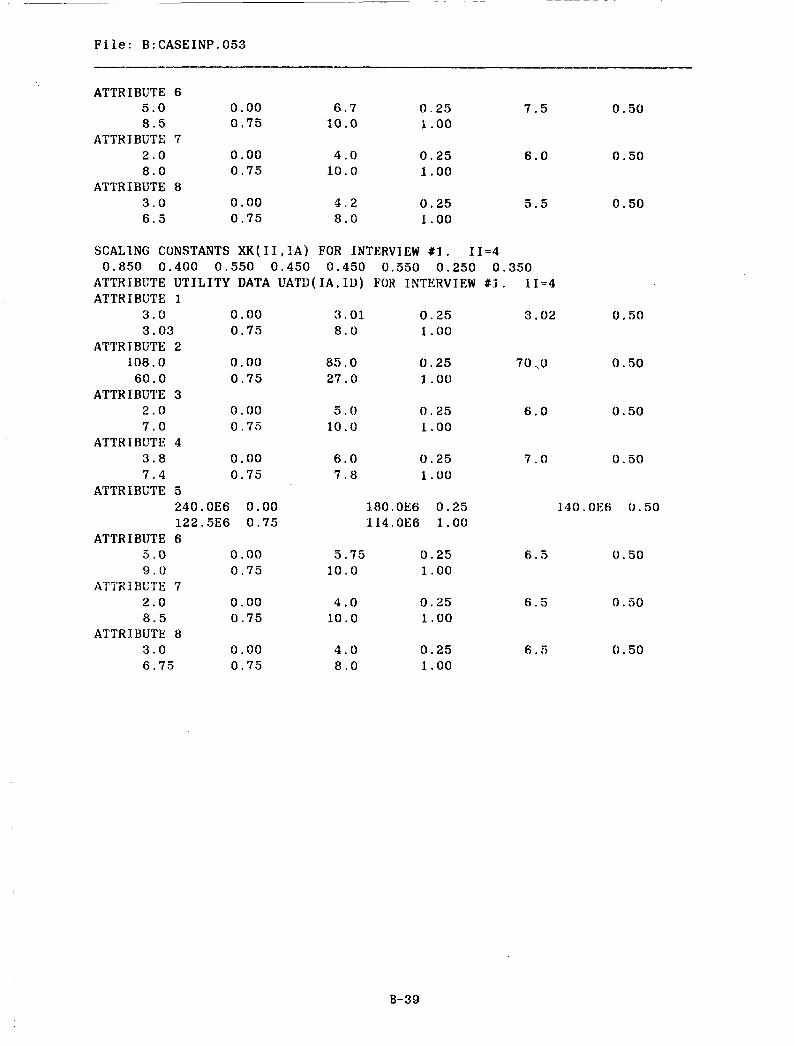
File: B:CASEINP.053

ATTRIBUTE 6 5.0 0.00 6.7 0.25 7.5 0.50 8 . 5 0 . 7 5 10.0 i .OO

2.0 0.00 4.0 0.25 6.0 0.50 8 . 0 0.75 10.0 1 .oo

3.0 0.00 4.2 0.25 5.5 0.50 6.5 0.75 8.0 1 .oo

ATTRIBUTE 7

ATTRIBUTE 8

SCALING CONSTANTS XK(I1,IA) FOR INTERVIEW # 3 . 11-4

ATTRIBUTE UTILITY DATA UATU(IA,ID) FOR INTERVIEW # I . 1I=4 ATTRIBUTE 1

0.850 0.400 0.550 0.450 0.450 0.550 0.250 0.350

3.0 0.00 3.01 0.25 3.02 0.50 3.03 0.75 8 . 0 1 .oo

ATTRIBUTE 2 108.0 0.00 85.0 0.25 70 ..O 0.50 60.0 0.75 27.0 1 .oo

ATTRIBUTE 3 2.0 0.00 5 . 0 0.25 6.0 0.50 7.0 0.75 10.0 1 .oo

3.8 0.00 6.0 0.25 7 . 0 0.50 7.4 0.75 7.8 1 .00

ATTHXHUTE 4

ATTKIRUTE 5 240.0E6 0.00 180.OE6 0.25 14O.OE6 0.50 122.5E6 0.75 114.OE6 1.00

ATTRIBUTE 6 9.0 0.00 5.75 0.25 6.5 0.50 9.0 0.75 10.0 1 .oo

2.0 0.00 4.0 0.25 6.5 0.50 8.5 0.75 10.0 1.00

3.0 0.00 4.0 0.25 6.5 0.50 6.75 0.75 8.0 1 .oo

ATTRIBUTE 7

ATTRIBUTE 8

B-39

File: B:CASEOUT.053

MATEUS

MULTIATTRJHUTE EVA1,UA'I'TON OF UTILITIES

RUN IDENTIFICATION NUMBER: 5 3 DIAGKOSTIC DISPLAY LEVEL: 0 NUMBER OF INDIVIDUALS: 4 NIJMBEN OF SYSTEMS : 16 NUMBER OF PROBABILl TY PATHS : 1 NUMBER OF ATTRIBUTES : 8 NUMBER OF ATTRIBCTE DArA: 10

ATTRIBLTE SCALING CONSTANTS X K ( 11, IB) FOR INDIVIDUAL ( I I = 1 ) .6700 .5000 .6200 .7000 .2000 .3303 .4500 .5000

SUM OF ATTRIBGTE SCALING CONSTANTS FOR INDIVIDUAL (I I = 1) 1s: 3 .9400 MASTER SCALiXG CONSTANT FOR INDlVlDS'AL (II= 1) IS: -.99702036 ATTRIBL"I"I' SCALIXG CONSTANTS XK(l7 ,TH) FOR INI)IViDL'A14 (IT= 2 )

.8000 . l o 0 0 .5000 .7000 . l o 0 0 .300C .2000 .6000 SIJM OF ATTRlBUTE SCALING CONS?'ANI'S FOR JNT)IVIDIJAL ( I I = 2 ) is 3.3000 MASTER SCALING CONSTANT FOR INDIVIDUAL (lI= 2) 1s: -.99424355

AT'I2iBl;TE SCAi* iXG CONSTAN'J'S XK( I1 , l a ) FOR 1NDIVI1)IJAL ( I I = 3 ) .6000 . l o00 .5000 .4000 .2000 .2000 .4000 .3000

SUM OF ATTRIRUTE SCALiNti CONSTANTS FOR lNDIVIDUA1, ( I 1 = 3 ) IS: 2.7000 MASTER SCALING CONSTANT FOR INDIVIDUAL ( l i = 3 ) IS: -.96579052 ATTRIRITE SCA1,ING CONSTANTS XK( JI , IH) FOR 1NI)IVIDlTAL ( I I= 4 )

.8500 .4000 .5500 ,4500 .4500 .5500 .2500 .3500 SKM 01: ATTRIBUTE SCALING CONSTANTS FOR INDIVIDUAL ( I ]= - 4) IS: 3.8500 MASTER SCALlNG CONSTANT FOR 1NDIVIDl:AL (II= 4) IS: -.99722735

MlJI,I'iATTKIBUTE; DECTSlON AXALYSTS RANKING OF ALTERNATIVE SYSTEMS ( I S )

BY 1NDIVIDUAI.S ( I I )

IS

1

2

3

4

5

6

7

8

11= 1 I i = 2 11= 3 11= UTILJTY RANK UTILITY RANK K'rIl,<'i'Y RANK tJ'l'11,ITY

.9549

.9153

.9807

.Y219

.92 16

.9726

.6848

,9812

11 .9045

14 .8924

5 .9526

12 .8546

13 .8730

7 .9501

16 .2747

4 .9601

11 ,856 i

12 .8178

7 .8976

15 .8016

13 .8096

8 -97 50

16 .4138

5 .9213

11 ,9664

12 .9278

8 .9856

15 .9376

13 .9586

6 .9748

16 .4969

5 .9793

4 11= HANK I;TTI,ITY RANK

10

14

4

13

12

8

16

7

B-40

File: B:CASEOUT.053

1. =

9

10

11

12

13

14

15

16

.9408

IS

1

2

3

4

5

6

7

8

9

10

:1 I

12

13

14

,9709

.9939

,9650

.9719

.8720

.9893

.9922

.9779

9

1

10

8

15

3

2

6

CH

,9621

.9859

.9492

.9577

.8617

.9758

.9860

.9276

4 .9074

2 .9559

9 .8662

6 .8860

14 .8032

3 .9710

1 .977 1

10 .9268

SQUARE = 56.45

7

3

10

9

14

2

1

4

MULTlATTRIBUTE L)l<CISlON ANALYSIS RANKING OF ALTERNATIVE SYSTEMS (IS)

RY GROUP DECISION RULES (IG)

IG = 1 ADDITIVE

VALUE RANK

.9205 11

.8883 13

.9541 5

.8789 14

.8907 12

.9531 7

.4675 16

.9605 4

.9520 8

.9821 2

.9359 10

.9488 9

.8590 15

.9819 3

IG = 2 XASH

VALUE RANK

.$I194 11

,8873 13

.95:35 5

.8772 14

.8889 12

.9528 7

.4435 16

.9602 4

.9516 8

.9820 2

.9350 10

.9480 9

.8582 15

.9818 3

,9675 9

.9927 2

.9630 11

.9795 6

,8989 15

.9913 3

.9928 1

.9822 5

DF = 15

IG = 3 XANK SUM

VALUE KANK

.3500 11

.2000 13

.6667 5

.1500 14

.2167 12

.5833 7

.oooo 16

.7267 4

-5833 7

.9333 2

.4ooo 10

.5833 7

.lo00 15

.8833 3

B-41

File: B:CASEOUT.053

15 .9870 1 .9870 1 .9833 1

i6 ,9537 6 ,9533 6 .e500 6

W = .9987 CHI SQUARE = 44.94 DF = 15

B-42

Documents

Spaceborne Power Systems Preference Analyses - NASA · JPL Publication 85-5 Spaceborne Power Systems Preference Analyses Volume II: Decision Analysis J.H. Smith A. Feinberg R.F. Miles,