SPACE-USE AND MOVEMENTS OF ADULT MALE WHITE …

SPACE-USE AND MOVEMENTS OF ADULT MALE WHITE-TAILED DEER IN

NORTHEASTERN LOUISIANA

by

TAYLOR NELSON SIMONEAUX

(Under the Direction of Michael J. Chamberlain and Karl V. Miller)

ABSTRACT

White-tailed deer (Odocoileus virginianus) are an important game species and the

number of adult males harvested has recently increased. Concurrently, increases in global

positioning system (GPS) technology for tracking animal movements have allowed detailed

studies of animal movements. Therefore, I used GPS-telemetry collars to investigate seasonal

and fine-scale movements and space use of adult male deer in northeastern Louisiana. I found

that males maintained largest space holdings in spring and fall/winter, followed by summer. I

also found that within the reproductive season, movements and space use were greatest during

the rut, followed by pre-rut and post-rut, and least during the non-breeding season. I modelled

movement rates and found that circadian period, breeding chronology, and refugia from hunting

were important variables for predicting movement rates. Finally, movement rates on a limited-

hunting refuge were more crepuscular than on open access hunting areas, suggesting deer may be

modifying behavior to avoid human predation.

INDEX WORDS: GPS, hunting pressure, Louisiana, movements, Odocoileus virginianus,

space use, white-tailed deer



by


B.S., B.S.F., Louisiana State University, 2012

A Thesis Submitted to the Graduate Faculty of The University of Georgia in Partial Fulfillment

of the Requirements for the Degree

MASTER OF SCIENCE

ATHENS, GEORGIA

2015

© 2015

Taylor Nelson Simoneaux

All Rights Reserved



by


Major Professor: Michael J. Chamberlain

Karl V. Miller

Committee: Robert G. Warren

John C. Kilgo

Electronic Version Approved:

Julie Coffield

Interim Dean of the Graduate School

The University of Georgia

May 2015

iv

DEDICATION

I would like to dedicate this thesis to those friends, family, scientists, and conservationists

who have made it possible for me to enjoy the great outdoors. The thrill of the hunt has

captivated countless generations of hunters and outdoorsman and I hope that those of us in the

present take the time to ensure that future generations are able to realize that same excitement.

With a little bit of luck, the information provided herein may prove useful to the completion of a

successful hunt.

v

ACKNOWLEDGEMENTS

First and foremost, I would like to thank my advisors, Dr. Michael Chamberlain and Dr.

Karl Miller. They have done more to advance my skills as a wildlife biologist and as a

professional than anyone else. Dr. Chamberlain especially has guided my education and career

since my undergraduate studies at LSU. Dr. Chamberlain, I certainly would not be where I am

now, nor going where I am in the future without your knowledge and support and for that, I

thank you. Additionally, Dr. Bradley Cohen has been invaluable in the completion of this thesis

and I thank him for the countless edits he made and the help he provided with data analysis.

David Osborn has become a close friend, and I certainly wouldn’t have been able to deal with all

of the logistics, paperwork, and red tape that he has helped with along the way. I would also like

to thank my committee members, Dr. Robert Warren and Dr. John Kilgo, who have helped

whenever called upon and Tom Prebyl for assistance in data analysis.

Special thanks to our funding sources, especially the Louisiana Department of Wildlife

and Fisheries. Mr. Scott Durham spent many hours trapping and assisting with various other

aspects of field work and his kindness and support is certainly appreciated. I would also like to

thank the Louisiana Wildlife and Fisheries Foundation, and the Central Louisiana and Northeast

Louisiana chapters of the Quality Deer Management Association. Finally, thanks to the United

States Fish and Wildlife Service, especially Kelly Purkey and John Dickson, for providing

housing, transportation, and allowing us access to a great field site.

Fellow researchers Elizabeth Cooney and Rebecca Shuman have played an integral role

in this project. They put up with me through years of field work in cramped quarters, in a remote

vi

location, and through seemingly endless difficulties and hard times. The shenanigans they

endured and oftentimes fueled (Cooney) certainly helped pass the time. The same thanks that

I’ve given them can also be applied to our field technicians. I wish Nathan Yeldell and Michael

Biggerstaff the best of luck as they are both pursuing their own master’s degrees. Zach

Haakonson and Jacob Thompson were always great help, and often the sources of great comedic

relief.

This project would have been impossible to complete without the help of local

landowners. Kirk Lee, Bruce McEarcharn, Ed Pardue, Ted Crawford, Randy and Ben Dukes, Dr.

Al Donald, Joe Scott, and Tracy Weems all graciously gave us access to their land for trapping

and monitoring of deer. I would like to thank all of the friends I made while I was doing field

work especially Miche Fandal and Curtis B. Their hospitality always came at an opportune time

and it was a pleasure getting to know them. Finally, the entire Norris family welcomed us in and

treated us like family. I only wish that I had met them sooner, and I hope that our friendship

continues for years to come.

I would be remiss if I did not mention my lab mates and friends I’ve made at UGA. Their

advice, encouragement, and most of all friendship has been a blessing. There are too many to list,

but they know who they are, and I am genuinely thankful for all they have done.

Last, but certainly not least, I would like to thank my family. I would not be the

outdoorsman that I am today without the knowledge of and exposure to the outdoors that my

cousins have afforded me since a young age. To everyone who took me hunting or fishing as a

child, especially Burchall, Arthur, and Bart Liles, and Joe Broyles, I can’t thank you enough. I’m

also thankful to those in my family who were close enough to my field site to welcome my

friends and me into their homes after long months in the field. My aunt, Susan, my grandmother,

vii

Emery, and my siblings Bradlee and Amanda have supported me with their love and support my

whole life and I can’t imagine where I would be without them. Finally, my deepest love and

thanks to my parents. While I’m sure they never understood it, they always encouraged me and

tolerated the numerous critters (both alive and dead) and mess associated with my love for the

outdoors. They have supported me in every way possible and have shaped me into the person I

am today.

viii

TABLE OF CONTENTS

Page

ACKNOWLEDGEMENTS .............................................................................................................v

LIST OF TABLES ...........................................................................................................................x

LIST OF FIGURES ....................................................................................................................... xi

CHAPTER

1 INTRODUCTION AND LITERATURE REVIEW .....................................................1

INTRODUCTION ...................................................................................................1

LITERATURE REVIEW ........................................................................................3

OBJECTIVES ..........................................................................................................8

STUDY AREA ........................................................................................................9

THESIS FORMAT ................................................................................................10

LITERATURE CITED ..........................................................................................11

2 SEASONAL AND FINE-SCALE MOVEMENTS AND SPACE-USE OF ADULT

MALE WHITE-TAILED DEER IN NORTHEASTERN LOUISIANA ....................19

ABSTRACT ...........................................................................................................20

INTRODUCTION .................................................................................................22

STUDY AREA ......................................................................................................24

METHODS ............................................................................................................25

RESULTS ..............................................................................................................28

DISCUSSION ........................................................................................................30

ix

MANAGEMENT IMPLICATIONS .....................................................................33


3 FINE-SCALE MOVEMENTS OF ADULT MALE WHITE-TAILED DEER IN

NORTHEASTERN LOUISIANA DURING THE HUNTING SEASON ..................48

ABSTRACT ...........................................................................................................49

INTRODUCTION .................................................................................................51

STUDY AREA ......................................................................................................53

METHODS ............................................................................................................54

RESULTS ..............................................................................................................60

DISCUSSION ........................................................................................................61

MANAGEMENT IMPLICATIONS .....................................................................63


x

LIST OF TABLES

Page

Table 2.1: Mean spring, summer, fall/winter, and annual 95% home range and 50% core area

size (ha) created using Kernel Density Estimators for adult male white-tailed deer in

northeastern Louisiana from 2013-2015 ............................................................................41

Table 2.2: Deer ID#, date of shift, and distance (km) between home range centroids for adult male

white-tailed deer exhibiting long-distance seasonal home range shifts in northeastern

Louisiana from 2013-2015 .................................................................................................41

Table 2.3: Excursions of adult male white-tailed deer outside of the 95% home range during the

spring and summer in northeastern Louisiana from 2013-2014 ........................................41

Table 3.1: Age distribution of collared adult male white-tailed deer included in the study. Data

collection occurred during the 2013-2014 and 2014-2015 hunting seasons in northeastern

Louisiana ............................................................................................................................72

Table 3.2: Mixed models used to evaluate relative importance of age class, period, macrohabitat,

hunting pressure and reproductive phase on the movement of adult male white-tailed deer

during the 2013-2014 and 2014-2015 hunting seasons in northeastern Louisiana ............72

Table 3.3: Akaike information criterion with small sample bias adjustment (AICc), number of

parameters (K), ∆AICc, Akaike weights (w) for candidate models (i) relating to variables

influencing step length of adult male white-tailed deer in northeastern Louisiana during

the 2013-2014 and 2014-2015 hunting seasons .................................................................73

xi

LIST OF FIGURES

Page

Figure 2.1: Weekly divisions, number of conceptions per week, and breeding status assigned to

each week of the hunting season used in calculations of weekly home ranges, core areas,

and movement rates of adult male white-tailed deer in northeastern Louisiana from 2013-

2015....................................................................................................................................42

Figure 2.2: Mean weekly home range ([ha] 95% utilization distribution, ± SE) calculated using

dynamic Brownian Bridge Movement Model for adult male white-tailed deer in northeastern

Louisiana during the 2013-2014 and 2014-2015 reproductive seasons............................42

Figure 2.3: Mean weekly core area ([ha] 50% utilization distribution, ± SE) calculated using


Louisiana during the 2013-2014 and 2014-2015 reproductive seasons.............................43

Figure 2.4: Mean weekly half-hour step lengths (± SE) for adult male white-tailed deer in

northeastern Louisiana during the 2013-2014 and 2014-2015 reproductive seasons ........43

Figure 2.5: Weekly 95% home range sizes calculated using DBBMM for adult male white-tailed

deer in northeastern Louisiana during the 2013-2014 and 2014-2015 reproductive

seasons. Note the variation in home range size, especially during the rut, and variation in timing

of home range size shifts....................................................................................................44

Figure 2.6: Weekly half-hour step lengths of adult male white-tailed deer in northeastern

Louisiana during the 2013-2014 and 2014-2015 reproductive seasons. Note the variation

in step lengths, especially during the rut, and variation in timing of shifts in step

xii

length..................................................................................................................................44

Figure 2.7: Seasonal 95% home range (Kernel) and weekly 95% home range and 50% core areas

(DBBMM) of two mature male white-tailed deer during the fall/winter of 2013-2014 in

northeastern Louisiana. Deer #33833’s weekly space use varied in both size and location

within his seasonal home range. Contrastingly, Deer #33829’s space use patterns

remained consistent throughout the season........................................................................45

Figure 2.8: An example of a long-distance seasonal home range shift by one adult male white-

tailed deer (ID# 33827) during the spring and summer of 2013 in northeastern Louisiana.

Concentric contours represent 95% and 50% Kernel home range estimates .....................46

Figure 2.9: Example of a non-breeding season excursion by an adult male white-tailed deer (ID#

35214) on March 28 and 29, 2014 in northeastern Louisiana. Green dots indicated

locations of the deer which show an excursion from his spring 95% Kernel home range

(green polygon) into his fall/winter home range (red polygon) .........................................47

Figure 3.1: Number of conceptions per week from October 1 to January 31 of 2013-2014 and

2014-2015. Based on these data, we assigned a reproductive phase to each day of our

study. We used this to calculate the effect of reproductive phase on the movements of 24

adult white-tailed deer in northeastern Louisiana during the 2013-2014 and 2014-2015

hunting seasons ..................................................................................................................74

Figure 3.2: Number of visitors based on self-clearing permits during the 2013-2014 and 2014-

2015 hunting seasons fitted to our predefined weeks using a 3 week moving window

analysis ...............................................................................................................................74

Figure 3.3: Map of the study area including the Tensas River National Wildlife Refuge (open-

access hunting), Greenlea unit (refuge), and adjacent private lands in northeastern

xiii

Louisiana. Locations (30-min) were obtained for 24 adult male white-tailed deer that

inhabited the area and movements were compared for movement within and outside the

Greenlea refuge ..................................................................................................................75

Figure 3.4: Mean (± SE) movement during crepuscular, day, and night periods for 24 adult male

white-tailed deer in northeastern Louisiana during the 2013-2014 and 2014-2015 hunting

seasons. We calculated movement as the linear distance between 2 consecutive 30 minute

locations .............................................................................................................................76

Figure 3.5: Mean (± SE) movements in different macrohabitats (agriculture, mature hardwoods,

and regenerating hardwoods) for 24 adult male white-tailed deer in northeastern

Louisiana during the 2013-2014 and 2014-2015 hunting seasons. We calculated

movement as the linear distance between 2 consecutive 30 minute locations ..................76

Figure 3.6: Mean (± SE) movements across the reproductive phase (non-breeding, pre-rut, rut,

and post rut sub-periods) for 24 adult male white-tailed deer in northeastern Louisiana

during the 2013-2014 and 2014-2015 hunting seasons. We calculated movement as the

linear distance between 2 consecutive 30 minute locations...............................................77

Figure 3.7: Mean (± SE) movements of different aged male white-tailed deer in northeastern

Louisiana during the 2013-2014 and 2014-2015 hunting seasons. We categorized deer as

adult (3.5 and 4.5 years old) and mature (5.5 years and older). We calculated movement

as the linear distance between 2 consecutive 30 minute locations ....................................77

Figure 3.8: Mean (± SE) movements in refuge and open-access hunting areas for adult male



locations .............................................................................................................................78

xiv

Figure 3.9: Movements of adult male deer during crepuscular, day, and night periods in open

access and refuge areas in northeastern Louisiana during the non-breeding, pre-rut, rut,

and post-rut reproductive phases in 2013-2014 and 2014-2015 hunting seasons as

predicted by our most parsimonious model .......................................................................78

Figure 3.10: Mean (±SE) percentage of time spent on refuge area (Greenlea) for harvested

(n=13) and un-harvested (n=11) adult male white-tailed deer in northeastern Louisiana

during the 2013-2014 and 2014-2015 hunting seasons .....................................................79

1

CHAPTER 1

INTRODUCTION AND LITERATURE REVIEW

INTRODUCTION

Understanding how animals maintain, traverse, and use space in their environment is a

prerequisite for successful wildlife management (Burt 1943, Fulbright and Ortega-Santos 2013).

The distribution of resources such as food, water, cover, and mates across a landscape influences

space use and movement patterns. The spatiotemporal dynamics of space use and movement

affect gene flow, population dynamics, disease transmission, and susceptibility to mortality

(Rosenberry et al. 1999, McCoy et al. 2005, Schauber et al. 2007, Karns et al. 2012).

Additionally, an understanding of space use can aid in determining species distributions (Araújo

and Guisan 2006), population estimates (Lancia et al. 2005), and resource use (Boyce et al.

2002).

Use of space and movements of white-tailed deer (Odocoileus virginianus; hereafter

deer) have been studied extensively. Published studies using very high frequency (VHF) radio-

telemetry data to calculate spatiotemporal dynamics of deer space use are extensive (Cochran

and Lord 1963, Tester et al. 1964, Beier and McCullough 1990, Kilpatrick et al. 2001, Brinkman

et al. 2005, Thayer et al. 2009). Although these studies have been insightful and set important

groundwork, VHF telemetry offers relatively low precision and sampling rates (Kochanny et al.

2009). As a result, phenomena occurring at finer temporal scales, such as seasonal home range

shifts and long distance movements of short duration, often go undetected (Kochanny et al.

2009). Technology for detecting animal locations using global positioning system (GPS)

2

technology has allowed detailed insights into these subtle changes in space use and movements

(Pépin et al. 2004, Frair et al. 2005, Sunde et al. 2009, Webb et al. 2010, Gulsby et al. 2011,

Karns et al. 2012, Little et al. 2014). For example, in a comparison of GPS and VHF technology

for determining the location of wild deer, Kochanny et al. (2009) found that home range size

calculations were influenced by differences in sampling intensity, wherein GPS collars recorded

locations that were missed using VHF telemetry. Further, these differences in sampling intensity

allowed more robust parameters and techniques to be used in home range size analyses

(Kochanny et al. 2009).

Deer movements and space use are affected by a multitude of environmental, ecological,

and anthropogenic factors (Kilpatrick et al. 2001, Brinkman et al. 2005, Kolodzinski et al. 2010,

Webb et al. 2010, Quinn et al. 2013, Tannenbaum et al. 2013). Perhaps most useful, studies

using GPS technology on cervids have revealed fine-scale changes in spatiotemporal dynamics

that could be useful in management. For example, studies examining responses to ephemeral

predation risk via hunter presence have found some cervids leave their home range and increase

their movements for short durations when disturbed (e.g., during “drive” hunts; Sunde et al.

2009), but do not exhibit this behavior under less-intensive hunting methods (e.g., during “stand”

hunts; Karns et al. 2012). Other studies have provided insight into common myths,

demonstrating neither localized weather events (precipitation, wind speed, etc.) nor moon phase

seem to affect fine-scale movements of deer (Webb et al. 2010).

Deer are the most popular game species in the United States with 11 million hunters

pursuing them and nearly $17 billion spent by big game hunters annually (U.S. Department of

the Interior 2011). For example, Louisiana deer hunters generate more than 50% of the total

economic effect and tax revenue collected by the state each year from recreational hunting

3

(Louisiana Department of Wildlife and Fisheries 2006). Therefore, funding for management

activities related to both game and nongame species depend on license sales and excise taxes on

deer hunters, making deer hunter satisfaction and participation critical to the management of

public and private lands. As more hunters target an older age class of male deer (Adams and

Ross 2014), it is increasingly important for biologists to understand the movement and space use

patterns of these mature males to enhance both management for these animals and the

satisfaction of those hunting them. Despite this importance, relatively few published studies have

explored the spatiotemporal dynamics of space use and movement of mature male deer. To better

manage the deer herds of tomorrow and their hunters, information on space use and fine scale

movements of mature male deer as they relate to breeding strategies, habitat preference, and the

impacts of hunting pressure, is needed.

LITERATURE REVIEW

An animal’s home range is defined as the area traversed by the individual in its normal

activities of food gathering, mating, and caring for young (Burt 1943). The concept of the home

range has been studied extensively, perhaps more than any other aspect of vertebrate ecology

(Stewart et al. 2011). Home ranges have been analyzed using a variety of methods, the most

common being minimum convex polygon and kernel density estimators (Fuller et al. 2005).

Minimum convex polygons are less accurate than kernel estimators, and neither takes into

account the temporal arrangement of spatial points (Kranstauber et al. 2012). With the recent

advances in GPS technology, acquisition of large data sets of animal locations is possible which

require new ways to analyze home ranges. For example, the dynamic Brownian bridge

movement model accounts for both location and time of the animal’s path, creating a utilization

distribution based on an animal’s activity (Kranstauber et al. 2012, Byrne et al. 2014).

4

Regardless of the method used to analyze deer home ranges, the habitat composition and

size of their home range is variable and seems dependent on a number of factors. Deer in

northern latitudes tend to have large seasonal shifts in home range location because temperature,

deer density, and snowfall can have a great effect on resource availability in northern climates

(Stewart et al. 2011). Conversely, southern latitudes have less environmental variation and as

such, sizes and location of deer home ranges tend to be more stable (Stewart et al. 2011). Males

tend to maintain larger home ranges, with expanded space use during the breeding season,

whereas females generally maintain smaller home ranges and reduce space use during parturition

(Ozoga et al. 1982, Beier and McCullough 1990, Sargent and Labisky 1995, D’Angelo et al.

2004, Webb et al. 2010). Age also seems to influence home range size, especially in males

(Webb et al. 2007, Hellickson et al. 2008). Older males generally have smaller home ranges than

young males (Hellickson et al. 2008), and yearlings often show long distance dispersal from their

natal home ranges, thereby greatly increasing their space use (Nelson and Mech 1984, McCoy et

al. 2005).

Previous studies in Louisiana using VHF telemetry (Thayer et al. 2009, Harrelson et al.

2012) found that home range sizes were largest in spring and smallest in summer. However,

these studies were not able to incorporate GPS technology, and despite the similarities in space

use observed, were conducted in different landscape types (Thayer et al. 2009, Harrelson et al.

2012). Whereas habitat is known to be one of the most important factors affecting deer

movements, (Beier and McCullough 1990, Vercauteren and Hygnstrom 1998, Lesage et al. 2000,

Brinkman et al. 2005, Long et al. 2005, Quinn et al. 2013), results from Thayer et al. (2009) and

Harrelson et al. (2012) suggest that space use may be more affected by other variables such as

age or sex. Although these results are useful, improvements in technology and methods of

5

analyzing data warrant revisiting space use patterns of deer in Louisiana. To date, there have

been no studies of adult male white-tailed deer space use in Louisiana or in the Lower

Mississippi Alluvial Valley using GPS collars.

Information detailing space use and movements of mature male deer is sparse, likely

because young males have traditionally been over-exploited leading to an under-representation

of mature males in many deer herds (Webb et al. 2007, Adams and Ross 2014, Olson 2014).

Advances in GPS technology have occurred simultaneously with an increase in the proportion of

mature male deer harvested (Clark et al. 2006, Kochanny et al. 2009, Adams and Hamilton 2011,

Adams and Ross 2014). As such, there have been recent studies using GPS telemetry to

investigate space use of mature male deer which have examined home range in relationship to

age (Webb et al. 2007), hunting pressure (Karns et al. 2012), breeding behavior (Tomberlin

2007, Basinger 2013, Olson 2014), and landscape structures (Quinn et al. 2013). Results from

these studies demonstrate that home range size varies temporally and spatially, as mature males

respond to changes in cover, forage availability, and biological cues (Webb et al. 2007, Karns et

al. 2012, Basinger 2013, Quinn et al. 2013, Olson 2014).

Understanding space use at fine temporal scales may be critical for informing deer

hunters of deer behavior during hunting season. Despite the fine spatial resolution of GPS

technology, little attention has been given to weekly shifts in spatial behavior by adult male

white-tailed deer. Female deer are in estrus for 24-48 hours (Knox et al. 1988), and in many

areas, initiation of estrus is often concentrated to a short (2-4 week) time period. As successful

males tend to females in estrus, increases in activity associated with breeding can change rapidly

due to searching, fighting, and pursuit of receptive females. For example, reported home range

size of adult males during the breeding season has ranged from 188 ha to 2,174 ha (Thayer 2009,

6

Foley 2011). These changes in movement patterns can have implications for deer observability

and harvest, deer-vehicle collisions (DVCs), crop damage, and gene flow (Vercauteren and

Hygnstrom 1998, Foley 2011, Gulsby et al. 2011, Little et al. 2014).

Burt (1943) excluded occasional movements outside of maintained areas from his

definition of home range. Both male and female deer are known to move outside of their home

ranges for brief periods (hereafter excursions). These excursions typically occur during the

breeding season and have been attributed to hunting pressure, mate searching, and/or breeding

activities (Tomberlin 2007, Kolodzinksi et al. 2010, Karns et al. 2011, Foley 2011, Basinger

2013). Excursions outside of the home range have potential to increase chances of mortality from

DVCs, hunter harvest, or disease transmission, have implications for gene flow, and are

important to understanding life history of the species. Olson et al. (2015) found that some adult

male deer also took excursions during spring and early summer in Pennsylvania. Specifically,

69% of males exhibited excursive behavior between April 6 and June 6, the cause of which was

unknown (Olson et al. 2015). Additionally, spring excursions have been found in white-tailed

deer populations in Georgia (D. Stone unpublished data) and Florida (Kilgo et al. 1996). The

paucity of research into this phenomenon, despite the wide geographical area it has been

documented across, requires a more detailed examination to further substantiate these spring-

time excursions.

As with space use, animal movements are influenced by the distribution of necessary

resources for that animal to survive and reproduce (Fuller et al. 2005). The coarse-scale data

available from VHF telemetry prevented detailed studies regarding movement patterns, as data

on a fine spatial and temporal scale are required. Movement patterns of deer are influenced by

many of the same factors as home range such as habitat, hunting pressure, and environmental

7

conditions, and are commonly analyzed using daily distance traveled and hourly movement rates

(D’Angelo et al. 2004, Pépin et al. 2004, Nelson et al. 2004, Webb et al. 2010, Basinger 2013).

However, detailed movement analyses such as cluster analysis, first passage time, and movement

models can be used to predict an animal’s behavior or to better delineate an animal’s response to

outside variables (Fauchald and Tveraa 2003, Nams 2005, Morales et al. 2004, Forester et al.

2007, Jonsen et al. 2007, Webb et al. 2009, Bacon et al. 2011, Foley 2011, Cristescu et al. 2014,

Little et al. 2014). The methods in the aforementioned studies have the ability to not only

describe movement patterns, but also to provide insight into the individual behavioral

characteristics of study animals and variation in responses across cohorts.

Studies using GPS telemetry have shown that deer movements change depending on

habitat, climate, season, and sex (Tomberlin 2007; Webb et al. 2009, 2010; Basinger 2013). For

example, in Oklahoma males moved more in spring during the 0500, 0600 and 1900 hours

compared to winter, but moved more during the 0900 and 1700 hours during winter than spring

(Webb et al. 2010). A study in southern Texas found that during the breeding season, males

revisited focal points once every 24 hours which were likely associated with female groups.

Apparently males were visiting these sites to assess receptiveness of females (Foley 2011).

Despite the study design or location, there has been a clear trend towards increased movements

of mature males during the rut, but previous studies have typically emphasized the average

movement, rather than variation of movements across individuals, despite a large standard error

often reported (Tomberlin 2007, Webb et al. 2009, 2010, Foley 2011, Basinger 2013, Olson

2014). Variations in movements may indicate differing behavioral characteristics of individual

deer such as mate searching, predator avoidance, and space holding tendencies (Brown 1974,

Foley 2011, Webb et al. 2007, Hellickson et al. 2008)

8

While many studies have described movement rates in regard to landscape features or

season, few have compared movements on areas of differing hunting pressure. Refuges which

limit or eliminate hunting on a particular area are often used in an attempt to protect deer

populations, and these refuges have been successful in doing so (Roseberry et al. 1969, Root et

al. 1988). Studies have shown that home range size and movement rates in refuge areas

decreased compared to their hunted counterparts (Kammermeyer and Marchinton 1976, Sargent

and Labisky 1995), although this trend has not been consistent across all studies, perhaps due to

availability of cover (Karns 2008). Despite the need to better understand deer movements in

relation to hunting pressure, relatively few studies using evolving technology have addressed this

subject. Studies using GPS telemetry to investigate hunting pressure on mature male deer have

not found hunting to affect deer home ranges, core areas, or excursions outside of the home

range in Maryland, although hunting pressure was possibly an influence on deer activity (Karns

et al. 2012). In another study investigating adult male response to hunting pressure in Oklahoma,

deer seemed to modify their behaviors to avoid detection by hunters (Little et al. 2014).

Additional research on the influence of hunting on fine-scale movements of mature male deer

may be an effective way to increase hunter efficiency and success through an improved

understanding of deer behavior.

OBJECTIVES

My objectives were to determine space use and movement patterns of adult male white-

tailed deer in northeastern Louisiana. Specifically, I investigated annual, seasonal and weekly

patterns of space use, non-breeding season excursions, and fine scale movements during the

reproductive season.

9

STUDY AREA

I conducted research on the Tensas River National Wildlife Refuge and adjacent private

lands located in northeastern Louisiana in the upper Tensas River Basin. The 30,750-ha refuge

was established in 1980 and was once predominately agriculture after being extensively logged.

Since acquisition by the United States Fish and Wildlife Service, forests on the refuge have been

allowed to grow into mature bottomland hardwood and swamps, and former agricultural fields

have been replanted in native hardwoods. The refuge was bordered almost entirely by agriculture

on all sides, making it an island of habitat for many species including deer and the federally

threatened Louisiana black bear (Ursus americanus luteolus).

The Tensas River and surrounding areas were once the location of the main channel of

the Mississippi River, and remains in the western Mississippi River floodplain. Topography on

the refuge was typical of a Mississippi River floodplain with ridge/swale, oxbow lakes, and

backwater swamps present. Overstory vegetation consisted of water oak (Quercus nigra), willow

oak (Q. phellos), hickory (Carya spp.), sweetgum (Liquidambar styraciflua), elm (Ulmus spp.),

ash (Fraxinus spp.), sugarberry (Celtis laevigata) with interspersed baldcypress (Taxodium

distichum) tupelo (Nyssa aquatica) swamps. The understory consisted of dwarf palmetto (Sabal

minor), poison ivy (Toxicodendron radicans), blackberry (Rubus spp.), trumpet creeper

(Campsis radicans), and greenbrier (Smilax spp.). Early to mid-successional hardwood plantings

were distributed throughout the refuge, which were established for carbon credits. These

hardwood plantings were initiated between 1985 and 2009 and comprised about 6,110 ha.

Agricultural crops grown on private lands surrounding the refuge included corn (Zea mays),

cotton (Gossypium hirsutum), soybeans (Glycine max) and rice (Oryza sp.). I concentrated

trapping efforts in the Greenlea Bend (hereafter Greenlea) closed area of the refuge. This area

10

was predominately planted hardwoods and agriculture, which was planted in milo (Sorghum sp.)

during the study period. Greenlea was closed to hunting with the exception of 3 staff-guided,

lottery deer hunts/year. Public access to Greenlea was restricted to a wildlife viewing drive

during daylight hours.

THESIS FORMAT

I have presented this thesis in manuscript format. Chapter 1 is an introduction and

literature review of white-tailed deer movement ecology. Chapter 2 is a descriptive study on the

space use and movement patterns of adult male white-tailed deer in northeastern Louisiana

including home ranges, core areas, and long-distance, fine-scale movements during the hunting

season, and long-distance, short-duration excursions outside of the home range. Chapter 3 is an

analysis of factors influencing fine-scale movement behavior of adult male white-tailed deer in

northeastern Louisiana.

11

LITERATURE CITED

Adams, K. and M. Ross. 2014. QDMA’s Whitetail Report 2014. Quality Deer Management

Association, Bogart, GA.

Adams, K. P., and R. J. Hamilton. 2011. Management history. Pages 355-377 in D.G. Hewitt,

editor. Biology and Management of White-tailed Deer, CRC Press, Boca Raton, FL.

Araújo, M. B., and A. Guisan. 2006. Five (or so) challenges for species distribution modelling.

Journal of Biogeography 33:1677-1688.

Bacon, M. M., G. M. Becic, M. T. Epp, and M. S. Boyce. 2011. Do GPS clusters really work?

Carnivore diet from scat analysis and GPS telemetry methods. Wildlife Society Bulletin

35:409-415.

Basinger, P. S. 2013. Rutting behavior and factors influencing vehicle collisions of white-tailed

deer in middle Tennessee. M.S. Thesis, University of Tennessee, Knoxville, 62 pp.

Beier, P., and D. R. McCullough. 1990. Factors influencing white-tailed deer activity patterns

and habitat use. Wildlife Monographs 109:1-51.

Boyce, M. S., P. R. Vernier, S. E. Nielsen, and F. K. Schmiegelow. 2002. Evaluating resource

selection functions. Ecological Modelling 157:281-300.

Brinkman, T. J., C. S. Deperno, J. A. Jenks, B. S. Haroldson, R. G. Osborn, and Hudson. 2005.

Movement of female white-tailed deer: effects of climate and intensive row-crop

agriculture. Journal of Wildlife Management 69:1099-1111.

Brown, B. A. 1974. Social organization in male groups of white-tailed deer. Pages 436-446 in V.

Geist and F. Walther, editors. The Behaviour of Ungulates and its Relation to

Management. Volume 1. International Union for the Conservation of Nature, Publication

24. Morges, Switzerland.

12

Burt, W. H. 1943. Territoriality and home range concepts as applied to mammals. Journal of

Mammalogy 24:346-352.

Byrne, M. E., J. C. McCoy, J. W. Hinton, M. J. Chamberlain, and B. A. Collier. 2014. Using

dynamic Brownian bridge movement modelling to measure temporal patterns of habitat

selection. Journal of Animal Ecology 83:1234-1243.

Clark, P. E., D. E. Johnson, M. A. Kniep, P. Jermann, B. Huttash, A. Wood, M. Johnson, C.

McGillivan, and K. Titus. 2006. An advanced, low-cost, GPS-based animal tracking

system. Rangeland Ecology and Management 59:334-340.

Cochran, W. W., and R. D. Lord, Jr. 1963. A radio-tracking system for wild animals. Journal of

Wildlife Management 27:9-24.

Cristescu, B., G. B. Stenhouse, and M. S. Boyce. 2014. Predicting multiple behaviors from GPS

radiocollar cluster data. Behavioral Ecology 2014:1-13

D'Angelo, G. J., C. E. Comer, J. C. Kilgo, C. D. Drennan, D. A. Osborn, and K. V. Miller. 2004.

Daily movements of female white-tailed deer relative to parturition and breeding.

Proceedings of the Southeastern Association of Fish and Wildlife Agencies 58:292–301.

Fauchald, P., and T. Tveraa. 2003. Using first-passage time in the analysis of area-restricted

search and habitat selection. Ecology 84:282-288.

Foley, A. M. 2011. Breeding behavior and secondary sex characteristics of male white-tailed

deer in southern Texas. Dissertation, Texas A&M University-Kingsville, 123 pp.

Forester, J. D., A. R. Ives, M. G. Turner, D. P. Anderson, D. Fortin, H. L. Beyer, D. W. Smith,

and M. S. Boyce. 2007. State-space models link elk movement patterns to landscape

characteristics in Yellowstone National Park. Ecological Monographs 77:285-299.

13

Frair, J. L., E. H. Merrill, D. R. Visscher, D. Fortin, H. L. Beyer, and J. M. Morales. 2005. Scales

of movement by elk (Cervus elaphus) in response to heterogeneity in forage resources

and predation risk. Landscape Ecology 20:273-287.

Fulbright, T. E., and J. A. Ortega-Santos. 2013. White-tailed Deer Habitat: Ecology and

Management on Rangelands. Texas A&M University Press. College Station, TX.

Fuller M. R., J. J. Millspaugh, K. E. Church, and R. E. Kenward. 2005. Wildlife Radiotelemetry.

Pages 377-417 in C.E. Braun, editor. Techniques for Wildlife Investigations and

Management. Sixth Edition. The Wildlife Society, Bethesda, Maryland, USA.

Gulsby, W. D., D. W. Stull, G. R. Gallagher, D. A. Osborn, R. J. Warren, K. V. Miller, and L. V.

Tannenbaum. 2011. Movements and home ranges of white‐tailed deer in response to

roadside fences. Wildlife Society Bulletin 35:282-290.

Harrelson, J. H., M. E. Byrne, M. J. Chamberlain, and S. Durham. 2012. Population

characteristics of a white-tailed deer herd in an industrial pine forest of north-central

Louisiana. Proceedings of the Southeastern Association of Fish and Wildlife Agencies

66:126-132.

Hellickson, M. W., T. A. Campbell, K. V. Miller, R. L. Marchinton, and C. A. DeYoung. 2008.

Seasonal ranges and site fidelity of adult male white-tailed deer (Odocoileus virginianus)

in southern Texas. Southwestern Naturalist 53:1-8.

Jonsen, I. D., R. A. Myers, and M. C. James. 2007. Identifying leatherback turtle foraging

behaviour from satellite telemetry using a switching state-space model. Marine Ecology

Progress Series 337:255-264.

14

Kammermeyer, K. E., and R. L. Marchinton. 1976. The dynamic aspects of deer populations

utilizing a refuge. Proceedings of the Southeastern Association of Game and Fish

Commissions 29:466-475.

Karns, G. R. 2008. Impact of hunting on adult male white-tailed deer behavior. M. S. Thesis,

North Carolina State University, Raleigh, 108 pp.

Karns, G. R., R. A. Lancia, C. S. DePerno, and M. C. Conner. 2011. Investigation of adult male

white-tailed deer excursions outside their home range. Southeastern Naturalist 10:39-52.

Karns, G. R., R. A. Lancia, C. S. DePerno, and M. C. Conner. 2012. Impact of hunting pressure

on adult male white-tailed deer behavior. Proceedings of the Southeastern Association of

Fish and Wildlife Agencies 66:120-125.

Kilgo, J. C., R. F. Labisky, and D. E. Fritzen. 1996. Directional long-distance movements by

white-tailed deer Odocoileus virginianus in Florida. Wildlife Biology 2:289-292.

Kilpatrick, H. J., S. M. Spohr, and K. K. Lima. 2001. Effects of population reduction on home

ranges of female white-tailed deer at high densities. Canadian Journal of Zoology 79:949-

954.

Knox, W. M., K. V. Miller, and R. L. Marchinton. 1988. Recurrent estrous cycles in white-tailed

deer. Journal of Mammalogy 69:384-386.

Kochanny, C. O., G. D. Delgiudice, and J. Fieberg. 2009. Comparing global positioning system

and very high frequency telemetry home ranges of white-tailed deer. Journal of Wildlife

Management 73:779-787.

Kolodzinski, J. J., L. V. Tannenbaum, L. I. Muller, D. A. Osborn, K. A. Adams, M. C. Conner,

W. M. Ford, and K. V. Miller. 2010. Excursive behaviors by female white-tailed deer

during estrus at two mid-Atlantic sites. American Midland Naturalist 163:366-373.

15

Kranstauber, B., R. Kays, S. D. LaPoint, M. Wikelski, and K. Safi. 2012. A dynamic Brownian

bridge movement model to estimate utilization distributions for heterogeneous animal

movement. Journal of Animal Ecology 81:738-746.

Lancia, R. A., W. L. Kendall, K. H. Pollock, and J. D. Nichols. 2005. Estimating the number of

animals in wildlife populations. Pages 106-153 in C. E. Braun, editor. Techniques for

Wildlife Investigations and Management. Sixth Edition. The Wildlife Society,

Bethesda, Maryland, USA.

Lesage, L., M. Crête, J. Huot, A. Dumont, and J. P. Ouellet. 2000. Seasonal home range size and

philopatry in two northern white-tailed deer populations. Canadian Journal of Zoology

78:1930-1940.

Little, A. R., S. Demarais, K. L. Gee, S. L. Webb, S. K. Riffel, J. A. Gaskamp, and J. L. Belant.

2014. Does human predation risk affect harvest susceptibility of white-tailed deer during

hunting season? Wildlife Society Bulletin 38:797-805.

Long, E. S., D. R. Diefenbach, C. S. Rosenberry, B. D. Wallingford, and M. D. Grund. 2005.

Forest cover influences dispersal distance of white-tailed deer. Journal of Mammalogy

86:623-629.

Louisiana Department of Wildlife and Fisheries. 2006. The economic benefits of fisheries,

wildlife and boating resources in the state of Louisiana. Baton Rouge, LA.

McCoy, J. E., D. G. Hewitt, and F. C. Bryant. 2005. Dispersal by yearling male white-tailed deer

and implications for management. Journal of Wildlife Management 69:366-376.

Morales, J. M., D. T. Haydon, J. Frair, K. E. Holsinger, and J. M. Fryxell. 2004. Extracting more

out of relocation data: building movement models as mixtures of random walks.

Ecology 85:2436-2445.

16

Nams, V. O. 2005. Using animal movement paths to measure response to spatial scale.

Oecologia 143:179-188.

Nelson, M. E., and L. D. Mech. 1984. Home-range formation and dispersal of deer in

northeastern Minnesota. Journal of Mammalogy 65:567-575.

Nelson, M. E., L. D. Mech, and P. F. Frame. 2004. Tracking of white-tailed deer migration by

global positioning system. Journal of Mammalogy 85:505-510.

Olson, A. K. 2014. Spatial use and movement ecology of mature male white-tailed deer in

northcentral Pennsylvania. Thesis, University of Georgia, Athens, 120 pp.

Olson, A. K., W. D. Gulsby, B. S. Cohen, M. E. Byrne, D. A. Osborn, and K. V. Miller. 2015.

Spring excursions of mature male white-tailed deer in north central Pennsylvania.

American Midland Naturalist in press.

Ozoga, J. J., L. J. Verme, and C. S. Bienz. 1982. Parturition behavior and territoriality in white-

tailed deer: impact on neonatal mortality. Journal of Wildlife Management 46:1-11.

Pépin, D., C. Adrados, C. Mann, and G. Janeau. 2004. Assessing real daily distance traveled by

ungulates using differential GPS locations. Journal of Mammalogy 85:774-780.

Quinn, A. C. D., D. M. Williams, and W. F. Porter. 2013. Landscape structure influences space

use by white-tailed deer. Journal of Mammalogy 94:398-407.

Root, B. G., E. K. Fritzell, and N. F. Giessman. 1988. Effects of intensive hunting on white-

tailed deer movement. Wildlife Society Bulletin 16:145-151.

Roseberry, J. L., D. C. Autry, W. D. Klimstra, and L. A. Mehrhoff, Jr. 1969. A controlled deer

hunt on Crab Orchard National Wildlife Refuge. Journal of Wildlife Management

33:791-795.

17

Rosenberry, C. S., R. A. Lancia, and M. C. Conner. 1999. Population effects of white-tailed deer

dispersal. Wildlife Society Bulletin 27:858-864.

Sargent, R. A., and R. F. Labisky. 1995. Home range of male white-tailed deer in hunted and

non-hunted populations. Proceedings of the Southeastern Association of Fish and

Wildlife Agencies 49:389-398.

Schauber, E. M., D. J. Storm, and C. K. Nielsen. 2007. Effects of joint space use and group

membership on contact rates among white‐tailed deer. Journal of Wildlife Management

71:155-163.

Stewart, K. M., R. T. Bowyer, and P. J. Weisberg. 2011. Spatial use of landscapes. Pages 181-

218. in D. G. Hewitt, editor. Biology and Management of White-tailed Deer. CRC Press,

Boca Raton, FL.

Sunde, P., C. R. Olesen, T. L. Madsen, and L. Haugaard. 2009. Behavioural responses of GPS-

collared female red deer Cervus elaphus to driven hunts. Wildlife Biology 15:454-460.

Tannenbaum, L. V., W. D. Gulsby, S. S. Zobel, and K. V. Miller. 2013. Where deer roam:

chronic yet acute site exposures preclude ecological risk assessment. Risk Analysis

33:789-799.

Tester, J. R., D. W. Warner, and W. W. Cochran. 1964. A radio-tracking system for studying

movements of deer. Journal of Wildlife Management 28:42-45.

Thayer, J. W., M. J. Chamberlain, and S. Durham. 2009. Space use and survival of male white-

tailed deer in a bottomland hardwood forest of southcentral Louisiana. Proceedings of the

Southeastern Association of Fish and Wildlife Agencies 63:1-6.

Tomberlin, J. W. 2007. Movement, activity, and habitat use of adult male white-tailed deer at

Chesapeake Farms, Maryland. Thesis, North Carolina State University, Raleigh, 104 pp.

18

U.S. Department of the Interior, U.S. Fish and Wildlife Service, and U.S. Department of

Commerce, U.S. Census Bureau. 2011 National Survey of Fishing, Hunting, and

Wildlife-Associated Recreation. http://www.census.gov/prod/2012pubs/fhw11-nat.pdf.

Vercauteren, K. C., and S. E. Hygnstrom. 1998. Effects of agricultural activities and hunting on

home ranges of female white-tailed deer. Journal of Wildlife Management 62:280-285.

Webb, S. L., D. G. Hewitt, and M. W. Hellickson. 2007. Scale of management for mature male

white- tailed deer as influenced by home range and movements. Journal of Wildlife


Webb, S. L., K. L. Gee, B. K. Strickland, S. Demarais, and R. W. DeYoung. 2010. Measuring

fine-scale white-tailed deer movements and environmental influences using GPS collars.

International Journal of Ecology 2010:1-12.

Webb, S. L., S. K. Riffell, K. L. Gee, and S. Demarais. 2009. Using fractal analyses to

characterize movement paths of white-tailed deer and response to spatial scale. Journal of

Mammalogy 90:1210-1217.

http://www.census.gov/prod/2012pubs/fhw11-nat.pdf

19

CHAPTER 2

SEASONAL AND FINE-SCALE MOVEMENTS AND SPACE-USE OF ADULT MALE

WHITE-TAILED DEER IN NORTHEASTERN LOUISIANA

Simoneaux, T. N, B. S. Cohen, E. A. Cooney, R. M. Shuman, M. J. Chamberlain and K. V.

Miller. To be submitted to Journal of Wildlife Management.

20

ABSTRACT

Although space use and movement patterns of white-tailed deer (Odocoileus virginianus)

have been studied extensively, investigations of fine-scale movements were not possible until the

development of global positioning system (GPS) technology. Further, relatively few studies have

investigated the movement ecology of mature male deer. Recent trends in hunter-harvest

selectivity have led to an increased representation of adult males in many populations and

management decisions affecting this segment of deer populations require an understanding of

their space use and movement ecology. Therefore, we obtained and analyzed GPS telemetry data

from 25 adult male deer (≥ 2.5 years old) in northeastern Louisiana to calculate annual, seasonal,

and weekly space use and movements. Annual home ranges and core areas averaged 484 ha (SE

= 105 ha) and 90 ha (SE = 22 ha), respectively. Males maintained larger home ranges during

spring (415 ± 91 ha) than fall/winter (333 ± 38 ha) or summer (208 ± 19 ha). During the rut,

mean weekly home range sizes varied from 38 ± 4 ha to 131 ± 20 ha and mean weekly core area

varied from 4.1 ± 0.5 ha to 15.4 ± 3.7 ha. Four of 25 adult males (16%) made non-breeding

season excursions outside of their home range and 4 adult males (16%) had distinct long-distance

shifts in home ranges among seasons. Although mean estimates of space use and movements are

similar to previous reports, we documented variation among individuals, particularly related to

rut-related movements and space use. Movements and space use of most males increased with

the onset of the breeding season, but decreased among other males. Further, weekly space use

shifted within the seasonal home range of some individuals but remained consistent among

others. Variation in movements and space use among individuals may reflect varied mate-

searching behaviors and social status and may impact susceptibility to harvest. These individual

21

variations may also confound camera survey population estimates and have implications for

management in areas of disease outbreak.

INDEX WORDS: GPS, Louisiana, movement, Odocoileus virginianus, space use, white-

tailed deer

22

INTRODUCTION

Understanding how animals maintain, traverse, and use space in their environment is a

prerequisite for successful wildlife management (Burt 1943, Fulbright and Ortega-Santos 2013).

Knowledge of space use can also aid in determining species distributions (Araújo and Guisan

2006), population estimates (Lancia et al. 2005), and resource use (Boyce et al. 2002). The

distribution of resources necessary for an animal to survive and reproduce influences space use

and movement patterns (Fuller et al. 2005). In white-tailed deer (Odocoileus virginianus;

hereafter deer), these spatio-temporal aspects of space use and movement affect population

dynamics, gene flow, and susceptibility to mortality (Rosenberry et al. 1999, McCoy et al. 2005,

Schauber et al. 2007, Little et al. 2014).

Space use and movements of deer have been characterized extensively. However, most

studies have been conducted using very high frequency (VHF) radio-telemetry on females or

immature males. While these studies have provided a foundational understanding of deer

movement ecology, VHF telemetry offers relatively low precision and sampling rates (Tester et

al. 1964, Beier and McCullough 1990, Kilpatrick et al. 2001, Brinkman et al. 2005, McCoy et al.

2005, Kochanny et al. 2009). Although recent trends in hunter-harvest selectivity have led to an

increased representation of adult males in many populations (Adams and Hamilton 2011, Adams

and Ross 2014), information detailing space use and movements of mature male deer is sparse,

likely because young males have traditionally been over-exploited leading to an under-

representation of mature males in many deer herds. Consequently, little attention has been given

to dynamic shifts in space use and movements of adult male white-tailed deer during the

breeding season, despite this time aligning with hunting season. Although space use and activity

are affected by many factors which can cause variation among individuals, adult males typically

23

increase their activity during the rut (Tomberlin 2007, Webb et al. 2009, 2010, Foley 2011,

Basinger 2013, Olson 2014). Movement patterns associated with the breeding season can change

rapidly as males establish dominance hierarchies, search for mates, and pursue and tend estrous

females. Climate, weather, age, and habitat also may affect the space use and activity of male

deer (Hirth 1977, Beier and McCullough 1990, Long et al. 2005, Hellickson et al. 2008, Webb et

al. 2010, Stewart et al. 2011, Quinn et al. 2013). These variables may influence activity patterns

across short temporal and spatial scales, affecting individual deer observability and harvest, deer-

vehicle collisions (DVCs), disease transmission, and gene flow (Vercauteren and Hygnstrom

1998, Schauber et al. 2007, Foley 2011, Gulsby et al. 2011, Little et al. 2014).

Both male and female deer have been reported to move outside of their home ranges for

brief periods (hereafter excursions). By definition, these movements are infrequent and are an

often overlooked aspect of movement ecology. Excursions typically occur during the breeding

season and are attributed to hunting pressure, mate searching, and/or breeding activities

(Tomberlin 2007, Kolodzinksi et al. 2010, Karns et al. 2011, Foley 2011, Basinger 2013).

Excursions may increase chances of mortality from DVCs or hunter harvest, contribute to

disease transmission, and have implications for gene flow. Excursions also may occur during

spring and early summer as a Pennsylvania study reported that 69% of collared males exhibited

excursive behavior between April 6 and June 6, the cause of which was unknown (Olson et al.

2015). Additionally, spring excursions have been found in white-tailed deer populations in

Georgia (D. Stone unpublished data) and Florida (Kilgo et al. 1996). The paucity of research into

this phenomenon, despite its widespread geographical representation, suggests that further

investigation is prudent.

24

As hunters increasingly desire opportunities to harvest mature male deer (Adams and

Ross 2014), it is important to understand the movement and space use patterns of this

demographic to enhance both management for these animals and the satisfaction of those hunting

them. Because movements and space holding tendencies of these animals can influence

individual and population-level characteristics such as observability, harvest susceptibility, and

potentially disease transmission, our objectives were to describe the seasonal and weekly space

use and movements of mature male deer on a study site in northeastern Louisiana.

STUDY AREA

We conducted research on the Tensas River National Wildlife Refuge and adjacent

private lands in northeastern Louisiana in the upper Tensas River Basin. The 30,750-ha refuge

was established in 1980 and was once predominately agriculture after being extensively logged.

Since acquisition by the United States Fish and Wildlife Service, forests on the refuge have been

allowed to grow into mature bottomland hardwood and swamps, and former agricultural fields

have been replanted in native hardwoods. The refuge was bordered almost entirely by agriculture

on all sides, making it an island of habitat for many species including deer and the federally

threatened Louisiana black bear (Ursus americanus luteolus).








25



were distributed throughout the refuge, which were established for carbon credits. These

hardwood plantings were initiated between 1985 and 2009 and comprised about 6,110 ha of the

refuge. During the study, agricultural crops grown on private lands surrounding the refuge

included corn (Zea mays), cotton (Gossypium hirsutum), and soybeans (Glycine max) and rice

(Oryza sp.).

METHODS

Data Collection

We captured 30 adult (≥2.5 years) male deer during January-March 2013 and 2014 using

a combination of drop nets (60’ x 60’ or 50’ x 50’), rocket nets (40’ or 60’) and free-range

darting with 3-ml Pneu-Dart transmitter darts (Pneu-Dart Inc., Williamsport, Pa and Daninject,

Børkop, Denmark). We anesthetized deer using a combination of ketamine (1.5 mg/kg)/xylazine

(2.5 mg/kg) when caught under a net or Telazol (5 mg/kg)/xylazine (2.5 mg/kg) when darting.

We estimated age by tooth wear and replacement (Severinghaus 1949). We fit deer with either

Lotek 7000mu GPS collars (Lotek Engineering, Ontario, Canada) or Followit Tellus® GPS

collars (Followit AB, Lindesberg, Sweden). Following instrumentation, we reversed anesthesia

using 3 ml of Tolazoline, half intravenously and half intramuscularly, and remained with animals

until ambulatory. Capture and handling protocol was approved by the University of Georgia

Institutional Animal Care and Use Committee, permit #A2012 06-006-Y3-A2.

Both types of collars allowed for remote data download via Ultra High Frequency (UHF)

signal. We programmed collars deployed in 2013 to collect locations at 13-hour intervals outside

of hunting season (Feb. 1-Sept. 30) and 30-minute intervals during the Louisiana state-wide

26

hunting season (Oct. 1-Jan. 31). This schedule allowed collars to retain sufficient battery life to

collect deer locations during both the 2013-2014 and 2014-2015 hunting seasons. We

programmed collars deployed in 2014 to collect locations every 13 hours (Lotek) or every 12

hours (Followit) from deployment to September 30 and every 30 minutes from October 1-

January 31. We chose to collect fine-scale location data during the hunting season as it

encompassed the reproductive season and we were interested in assessing space use and

movements relative to breeding activity. We monitored VHF signals once/week to determine

activity mode of the animal (active, mortality, low battery). We downloaded data from the

collars at the beginning and end of each hunting season.

Analysis of Space Use

We imported data into ArcGIS 10.2 (Environmental Systems Research Institute, Inc.,

Redlands, Ca) and projected locations in Universal Transverse Mercator (UTM) North American

Datum (NAD) 1983 zone 15N (meters). We censored data to eliminate non-fix and impossible

locations. We defined seasons as spring (Feb. 15-May 31), summer (June 1- Sept. 31), and

fall/winter (Oct. 1-Feb. 14). We chose these seasons based on deer biology (pre-fawning,

fawning, and breeding seasons, respectively; see Thayer et al. 2009). We used all locations taken

from capture in the late fall/winter or early spring through the end of the following fall/winter

season to calculate annual home ranges and core areas; however, we selected a subset of fine-

scale data taken during the fall/winter to match data acquisition rates during other seasons.

Because we were interested in short temporal shifts in space use and movement

associated with breeding behavior, we divided the reproductive season into weekly periods, from

October 1-7 through January 27-31. We classified these weekly intervals relative to rutting

27

activity (non-breeding, pre-rut, rut or post-rut), based on conception dates determined from

concurrent research on the same study site (Figure 2.1).

We calculated annual and seasonal 95% home ranges and 50% core areas for each year

using 12- or 13-hour location data using Kernel Density Estimator (KDE) in program R, version

3.0.2 (R Core Team 2013), package “adehabitat” (Calenge 2006). If we had 2 years of data for a

deer, we used the home range and core area for each year to calculate a mean for that deer. We

then calculated a mean and standard error for annual and seasonal home ranges and core areas

for all deer. To describe behavior of deer that made long-distance seasonal home range shifts, we

measured the distance between home range centroids and calculated the mean distance between

centroids for any deer whose home ranges between seasons were separated by at least 1.6 km.

For deer with bi-modal home ranges which shifted during a predefined season (spring, summer,

or fall/winter), a home range was generated for each cluster of points, which were then combined

to calculate a composite home range size for that deer during that season.

We used locations recorded every 30 minutes to calculate weekly home ranges and core

areas during the reproductive season. We used a dynamic Brownian bridge movement model

(DBBMM, Kranstauber et al. 2012) to estimate utilization distributions (UD) and construct

weekly home ranges and core areas (95% and 50% UD isopleth) during the reproductive season

using the R package “move” (Kranstauber and Smolla 2015). A UD is a spatial probability

distribution that describes the probability of an animal occurring in a specific location during the

sampling period. Because the Brownian-bridge-based UD estimation is based on the movement

trajectory and behavior of an individual, these methods perform well on high volume GPS

datasets that often violate the independence assumptions underlying traditional UD estimation

methods (e.g., kernel density method) which are based solely on the spatial pattern of relocations

28

(Horne et al. 2007). We used a margin size, window size, and dimension size of 5, 21, and 85,

respectively, for DBBMM based on suggestions by Kranstauber et al. (2012). We calculated

mean and standard error each week for both home range and core area. As some deer were lost

because of harvest, we only calculated weekly home ranges and core areas using complete weeks

leading up to their harvest.

Analysis of Movements and Excursions

We calculated half-hour step length (the linear distance between consecutive points) for

each deer during each week between October 1 and January 31 using the command “movement

pathmetrics” in Geospatial Modeling Environment (GME), version 0.7.3.0 (Beyer 2012). We

calculated mean step length for each deer per week, and then summarized the sample data as

mean and standard error step length per week. As some deer were lost to harvest, we only

calculated step lengths up to the day before harvest.

To describe non-breeding season excursions, we used a methodology similar to that

outlined in Olson et al. (2015). Specifically, we defined excursions as a movement ≥ 1.6 km

outside of the 95% seasonal kernel home range for >13 hours and <7 days. This framework

allowed us to identify excursions while ensuring ≥2 locations (13-hour data locations) were

taken to minimize the chance of an erroneous GPS location being identified as an excursion.

RESULTS

We captured 14 adult males in 2013 and 16 in 2014. We lost 5 deer to mortality or collar

malfunction, resulting in 25 data-sets. We monitored 8 deer during both years of the study,

providing us with a total sample of 24-25 deer depending on season.

Mean annual home range was 484 ± 105 ha (range 188-2,659 ha), whereas mean annual

core area was 90 ± 22 ha (range 22-551 ha). Mean seasonal home range size was largest in

29

spring (415 ± 91 ha, range 92-2,167 ha) followed by fall/winter (333 ± 38 ha, range 30-853 ha)

and summer (208 ± 19 ha, range 76-407 ha). Likewise, core areas were largest in spring (87 ± 20

ha, range 21-470 ha) followed by fall/winter (73 ± 9 ha, range 6-221 ha) and summer (44 ± 5 ha,

range 15-87 ha; Table 2.1).

Mean weekly home range size during the reproductive season was 77 ± 7 ha. Mean

weekly home range was smallest during the non-breeding season (Week 2; 38 ± 4 ha, range 17-

99 ha) and largest during rut (Week 14; 131 ± 20 ha, range 22-456 ha; Figure 2.2). Mean weekly

core area size averaged 8.4 ± 1.0 ha. Mean weekly core area also was smallest during the non-

breeding season (week 1; 4.1 ± 0.5 ha, range 1-12 ha) and largest during the rut (week 14; 15.4 ±

3.7 ha, range 3-62 ha; Figure 2.3). Likewise, mean weekly step length was least during the non-

breeding season (week 2; 57 ± 3 m) and greatest during the rut (week 12; 125 ± 11 m) with an

overall mean half hour step length of 83 ± 5 m (Figure 2.4).

We identified 4 distinct behavioral patterns in movements and space use that differed

among individuals: temporal variation in weekly home range sizes and movement rates, spatial

variation in weekly home ranges, long-distance seasonal home range shifts, and non-breeding

season excursions. Weekly home range sizes and movement rates showed a pronounced degree

of individual variation. While weekly space use and movements generally increased during the

rut, the timing of these increases were inconsistent across individuals and some animals

decreased their movement rates and home range sizes during the rut (Figures 2.5 and 2.6).

Among individuals, the weekly patterns of space use within their seasonal home ranges differed.

Space use by some individuals shifted spatially throughout the reproductive season, whereas

others were consistent in their space use throughout the reproductive season (Figure 2.7).

30

Four deer demonstrated long-distance seasonal home range shifts averaging 9.58 km.

One of these deer (ID# 33827) maintained 2 distinct seasonal home ranges, 10.7 km apart, during

each of the 2 years he was monitored. Following capture in February 2013, he maintained a

home range size of 175 ha until March 18. By March 19 he moved northeast 10.7 km and

remained there until August 6. On August 7, he moved southeast back to his original area and

remained there from August 9 to March 8, 2014. During 2014, this deer again traveled to his

summer range on March 18 and remained there until returning July 28 (Figure 2.8). Three other

deer demonstrated long-distance seasonal home range shifts on April 1, April 18, and November

5 averaging 8.19 km (Table 2.2).

Four of 25 deer (16%) took 5 non-breeding season excursions during the spring (n = 4)

and summer (n = 1). Mean excursion distance from the home range boundary was 3.05 km

(range 1.94-4.94 km). Mean total distance travelled per excursion was 6.73 km (range 5.06-10.12

km). Mean duration of excursions was 31 hours (range 13-52), although these excursions

occurred while collars were recording locations every 12 or 13 hours (Table 2.3). One excursion

was from a deer (ID# 35214) that had a bi-modal home range. This excursion occurred from the

spring home range into the fall/winter home range (Figure 2.9).

DISCUSSION

We observed annual home range and core area sizes of 484 ± 105 ha and 90 ± 22 ha,

respectively. We noted that space use fluctuated seasonally, with males maintaining larger spaces

during spring and fall/winter, and smaller spaces during summer. Additionally, 4 males (16%)

shifted the centroid of their home range at least 1.6 km between seasons. During the hunting

season, males increased space use and movements, both peaking during the rut. Lastly, 4 males

31

(16%) demonstrated excursive movements during the non-breeding seasons, averaging 3.05 km

from their home range boundary.

Our estimates of home range and core area size were within the reported home range

sizes of adult male deer (Webb et al. 2007, Tomberlin 2007, Hellickson et al. 2008, Karns 2008,

Foley 2011, Olson 2014). However, the individual variation in space use and movements we

observed across individuals was surprising. We found seasonal home ranges to be a minimum

size of 30 ha for an individual male in fall/winter up to a maximum of 2,167 ha for a different

male in spring. Additionally, annual home range sizes varied greatly among individuals, ranging

from 188 ha to 2,659 ha. Pronounced variation in space use and movements of deer are

commonly seen across cohorts or from studies across differing environmental conditions. For

example, Vercauteren and Hygnstrom (1998) reported a female deer in Nebraska with a home

range of 21 ha in an agricultural landscape before corn harvest and Lesage et al. (2000) reported

mean summer home range size of yearling males in Quebec to be up to 7,484 ha. However, the

variability we observed has rarely been reported within individual studies.

Whereas adult male deer generally increased space use and movements during the rut,

there also was a large amount of individual variation among deer during that time. Home range

sizes and movement rates were consistent among individuals during the non-breeding weeks

until late November/early December. However, males apparently responded differently to the

onset of the pre-rut and rut. Space use and movements by most males increased during the pre-

rut and rut, although the timing and magnitude of the increase varied among individuals.

Contrastingly, home range sizes of a subset of individuals decreased during the pre-rut and rut

and movement rates remained similar to rates during the non-breeding period. During the post-

rut, movements and space use appeared to converge toward non-breeding-phase rates. In addition

32

to inter-individual variation in space use and rate of movement, the location of weekly space use

within the seasonal home range changed frequently with some individuals but not with others.

For some males we observed little overlap in week-to-week space use; these males

variably vacated and occupied portions of their home range at intervals during the breeding

season. Inter-individual variations in movements and space use may be related to differing mate-

searching strategies, which may be linked to social status or shifting resource availability (Brown

1974, Hellickson et al. 2008, Foley 2011). Further, variable space use during the rut contrasts

with Foley’s (2011) observations from South Texas indicating that males often re-visited focal

points during the rut. In that study, focal points were often associated with supplemental feeders

and males presumably were shifting among female groups focused at these areas of concentrated

resource availability. Contrastingly, dispersed distribution of females would suggest that males

may variably concentrate movements associated with individual females or female groups within

their seasonal home range with the associated risk of encountering known or novel rival males.

Alternatively, males may focus space use on a small portion of their seasonal range, weighing

reduced access to females with reduced risk of encounters with rivals.

Little et al. (2014) used observability as a surrogate for harvest susceptibility and found

that increased movement rates of individual deer increased their observability. Likewise, the

weekly shifts in space use we observed may have implications for deer observability and harvest.

Additionally, increases or decreases in movements or space use may confound efforts to estimate

population abundance (Jacobson et al. 1997) and/or pattern deer movements for capture or

harvest. Finally, although Foley (2011) reported that 5% of deer had multiple home ranges in

Texas, southern deer are relatively sedentary. We observed a frequency of bi-modal home ranges

in males that has not been reported previously from southern regions.

33

Including our findings, non-breeding season excursions have now been observed in

Florida (Kilgo et al. 1996), Pennsylvania (Olson et al. 2015), Georgia (D. Stone unpublished

data), and Louisiana. Theories as to the cause of excursions include a return to natal range,

female aggression associated with parturition, and trips to mineral sites, although these causes

were deemed unlikely (Kilgo et al. 1996, Olson et al. 2015). We found no evidence suggesting

that the excursions we documented were influenced by any of these factors, although 1 excursion

was from a deer (deer ID# 35214) with a bi-modal home range. This spring-time excursion

occurred from the deer’s spring home range into the deer’s fall/winter home range (Figure 2.9).

It is likely that these excursions occur across the distribution of the white-tailed deer, but further

research into this phenomenon is needed.

High inter-individual variability in seasonal home range size, long-distance home range

shifts, and excursions may impact the success of deer management strategies. Data from studies

in South Texas suggest that space use by mature male deer is not consequential given their small

annual home ranges and relative stability of home ranges relative to land ownership patterns

(Webb et al. 2007). However, our data suggest that these trends are not ubiquitous and variability

in spatio-temporal movement behavior of mature male deer should be further investigated,

particularly in areas where public and private land ownership patterns are smaller and highly

fragmented.

MANAGEMENT IMPLICATIONS

Management for white-tailed deer often involves camera trapping to identify males,

estimate age and sex ratios, and determine population size or density (Jacobson et al. 1997).

Home range shifts and long distance movements by males may bias these calculations by

counting males during the survey that are would not be present during subsequent management

34

of the area. In addition, behaviors related to space use and movements can affect observability

and susceptibility to harvest (Little et al. 2014). Management strategies to increase representation

of mature males in deer herds are increasing in popularity (Adams and Hamilton 2011). The

variations in movements and space use we found among males suggest that in some regions, land

ownerships or small groups of ownerships may meet with marginal management success as the

animals they have been managing may be harvested on properties with differing management

strategies. Large-scale deer management cooperatives, or regulations at the county or deer

management unit level, may be necessary to envelop the range of variability in space use by

mature males that we observed.

A deer herd with a high percentage of wide-ranging adult males may have implications

for management in areas of disease outbreaks, especially chronic wasting disease (CWD). To

prevent the spread of this disease, populations are reduced to attempt to contain the outbreak of

CWD to a small area (Williams et al. 2002). Further research may be required in areas with

CWD to determine the extent of variations in movements, space use, and excursions. If long-

distance movements and shifts in space use occur, this may justify an increase in the size of these

containment zones for CWD. Further, state agencies may want to preemptively research deer

movement ecology locally in an attempt to have a plan in place should a CWD outbreak occur.

35

LITERATURE CITED

Adams, K. and M. Ross. 2014. QDMA’s whitetail report 2014. Quality Deer Management

Association, Bogart, Georgia.


editor. Biology and management of white-tailed deer, CRC Press, Boca Raton, FL.

Araújo, M. B., and A. Guisan. 2006. Five (or so) challenges for species distribution modelling.

Journal of Biogeography 33:1677-1688.

Basinger, P. S. 2013. Rutting behavior and factors influencing vehicle collisions of white-tailed

deer in middle Tennessee. M.S. Thesis, University of Tennessee, Knoxville.



Beyer, H. L. 2012. Geospatial Modelling Environment. Available at

http://www.spatialecology.com/gme.

Boyce, M. S., P. R. Vernier, S. E. Nielsen, and F. K. Schmiegelow. 2002. Evaluating resource

selection functions. Ecological Modelling 157:281-300.

Brinkman, T. J., C. S. Deperno, J. A. Jenks, B. S. Haroldson, and R. G. Osborn. 2005. Movement

of female white-tailed deer: effects of climate and intensive row-crop agriculture. Journal

of Wildlife Management 69:1099-1111.


Geist and F. Walther, editors. The behaviour of ungulates and its relation to management.

International Union Conservation of Nature Publications 24, Morges, Switzerland. pp.

436-446.

36

Burt, W. H. 1943. Territoriality and home range concepts as applied to mammals. Journal of

Mammalogy 24:346-352.

Calenge, C. 2006. The package adehabitat for the R software: a tool for the analysis of space and

habitat use by animals. Ecological Modelling 197:516-519.

Foley, A. M. 2011. Breeding behavior and secondary sex characteristics of male white-tailed

deer in southern Texas. Dissertation, Texas A&M University-Kingsville, 123 pp.

Fulbright, T. E., and J. A. Ortega-Santos. 2013. White-tailed deer habitat: ecology and

management on rangelands. Texas A&M University Press. College Station, TX.

Fuller M. R., J. J. Millspaugh, K. E. Church, and R. E. Kenward. 2005. Wildlife radiotelemetry.

Pages 377-417 in C.E. Braun, editor. Techniques for wildlife investigations and

management. Sixth Edition. The Wildlife Society, Bethesda, Maryland, USA.







Hirth, D. H. 1977. Social behavior of white-tailed deer in relation to habitat. Wildlife

Monographs 53:3-55.

Horne, J. S., E. O. Garton, S. M. Krone, and J. S. Lewis. 2007. Analyzing animal movements

using Brownian bridges. Ecology 88:2354-2363.

Jacobson, H. A., J. C. Kroll, R. W. Browning, B. H. Koerth, and M. H. Conway. 1997. Infrared-

triggered cameras for censusing white-tailed deer. Wildlife Society Bulletin 25:547-556.

37

Karns, G. R. 2008. Impact of hunting on adult male white-tailed deer behavior. M. S. Thesis,

North Carolina State University, Raleigh.

Karns, G. R., R. A. Lancia, C. S. DePerno, and M. C. Conner. 2011. Investigation of adult male

white-tailed deer excursions outside their home range. Southeastern Naturalist 10:39-52.

Kilgo, J. C., R. F. Labisky, and D. E. Fritzen. 1996. Directional long-distance movements by

white-tailed deer Odocoileus virginianus in Florida. Wildlife Biology 2:289-292.



954.

Knox, W. M., K. V. Miller, and R. L. Marchinton. 1988. Recurrent estrous cycles in white-tailed

deer. Journal of Mammalogy 69:384-386.

Kochanny, C. O., G. D. Delgiudice, and J. Fieberg. 2009. Comparing global positioning system

and very high frequency telemetry home ranges of white-tailed deer. Journal of Wildlife


Kolodzinski, J. J., L. V. Tannenbaum, L. I. Muller, D. A. Osborn, K. A. Adams, M. C. Conner,

W. M. Ford, and K. V. Miller. 2010. Excursive behaviors by female white-tailed deer

during estrus at two mid-Atlantic sites. American Midland Naturalist 163:366-373.

Kranstauber, B., R. Kays, S. D. LaPoint, M. Wikelski, and K. Safi. 2012. A dynamic Brownian

bridge movement model to estimate utilization distributions for heterogeneous animal

movement. Journal of Animal Ecology 81:738-746.

Kranstauber, B. and M. Smolla. 2015. Move: Visualizing and analyzing animal track data.

http://computational-ecology.com/main-move.html.

http://computational-ecology.com/main-move.html

38

Lancia, R. A., W. L. Kendall, K. H. Pollock, and J. D. Nichols. 2005. Estimating the number of

animals in wildlife populations. Pages 106-153 in C.E. Braun, editor. Techniques for

wildlife investigations and management. Sixth Edition. The Wildlife Society, Bethesda,

Maryland, USA.



78:1930-1940.






86:623-629.

McCoy, J. E., D. G. Hewitt, F. C. Bryant, and Morgart. 2005. Dispersal by yearling male white-

tailed deer and implications for management. Journal of Wildlife Management 69:366-

376.

Olson, A. K. 2014. Spatial use and movement ecology of mature male white-tailed deer in

northcentral Pennsylvania. Thesis, University of Georgia, Athens, 120 pp.

Olson, A. K., W. D. Gulsby, B. S. Cohen, M. E. Byrne, D. A. Osborn, and K. V. Miller. 2015.

Spring excursions of mature male white-tailed deer in north central Pennsylvania.

American Midland Naturalist in press.



39

R Core Team. 2013. R: a language and environment for statistical computing. R foundation for

Statistical Computing, Vienna, Austria.

Rosenberry, C. S., R. A. Lancia, and M. C. Conner. 1999. Population effects of white-tailed deer

dispersal. Wildlife Society Bulletin 27:858-864.

Severinghaus, C. W. 1949. Tooth development and wear as criteria of age in white-tailed deer.

Journal of Wildlife Management 13:195-216.



71:155-163.


218. in D.G. Hewitt, editor. Biology and management of white-tailed deer. CRC Press,

Boca Raton, Fl.



Thayer, J. W., M. J. Chamberlain, and S. Durham. 2009. Space use and survival of male white-

tailed deer in a bottomland hardwood forest of southcentral Louisiana. Proceedings of the

Southeastern Association of Fish and Wildlife Agencies 63:1-6.





40


white- tailed deer as influenced by home range and movements. Journal of Wildlife







Mammalogy 90:1210-1217.

Williams, E. S., M. W. Miller, T. J. Kreeger, R. H. Kahn, and E. T. Thorne. 2002. Chronic

wasting disease of deer and elk: a review with recommendations for management. The


41

Table 2.1. Spring, summer, fall/winter, and annual 95% home range (HR)and 50% core area

(CA) size (ha) created using Kernel Density Estimators for adult male white-tailed deer in

northeastern Louisiana from 2013-2015.

Spring Summer Fall/Winter Annual

Statistic HR CA HR CA HR CA HR CA

Mean 415 87 208 44 333 73 484 90

SE 91 20 19 5 38 9 105 22

n 25 25 25 25 24 24 25 25

Min 92 21 76 15 30 6 188 22

Max 2167 470 407 87 853 221 2659 551

Table 2.2. Deer ID#, date of shift, and distance (km) between home range centroids for adult

male white-tailed deer exhibiting long-distance seasonal home range shifts in northeastern

Louisiana from 2013-2015.

Deer ID# Date of Shift Distance Between Centroids

33827 3/18/2013 10.69

33827 8/7/2013 10.76

33827 3/18/2014 10.68

33827 7/28/2014 10.35

33837 4/1/2014 4.19

35214 11/5/2014 5.50

3598 4/18/2014 14.88

Mean 9.58

Table 2.3. Excursions of adult male white-tailed deer outside of the 95% home range during the

spring and summer in northeastern Louisiana from 2013-2014.

Deer

ID# Start Date End Date

Total

Time (hrs)

Distance from edge

95% HR (km)

Total path distance

traveled (km)

33840 3/27/2013 3/29/2013 52 1.94 5.57

33838 4/4/2013 4/5/2013 39 1.98 5.06

33830 4/9/2013 4/11/2013 39 3.03 6.07

33830 6/1/2013 6/1/2013 13 3.35 6.83

35214 3/28/2014 3/29/2014 13 4.94 10.12

Mean

31.2 3.05 6.73

42

Figure 2.1. Weekly divisions, number of conceptions per week, and breeding status assigned to

each week of the hunting season used in calculations of weekly home ranges, core areas, and

movement rates of adult male white-tailed deer in northeastern Louisiana from 2013-2015.

Figure 2.2. Mean weekly home range ([ha] 95% utilization distribution, ± SE) calculated using


Louisiana during the 2013-2014 and 2014-2015 reproductive seasons.

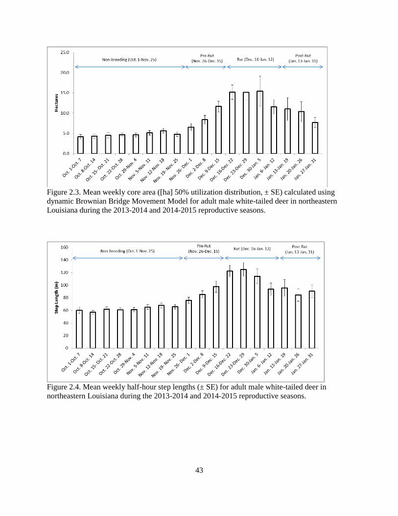
43

Figure 2.3. Mean weekly core area ([ha] 50% utilization distribution, ± SE) calculated using


Louisiana during the 2013-2014 and 2014-2015 reproductive seasons.

Figure 2.4. Mean weekly half-hour step lengths (± SE) for adult male white-tailed deer in

northeastern Louisiana during the 2013-2014 and 2014-2015 reproductive seasons.

44

Figure 2.5. Weekly 95% home range sizes calculated using DBBMM for adult male white-tailed

deer in northeastern Louisiana during the 2013-2014 and 2014-2015 reproductive seasons. Note

the variation in home range size, especially during the rut, and variation in timing of home range

size shifts.

Figure 2.6. Weekly half-hour step lengths of adult male white-tailed deer in northeastern

Louisiana during the 2013-2014 and 2014-2015 reproductive seasons. Note the variation in step

lengths, especially during the rut, and variation in timing of shifts in step lengths.

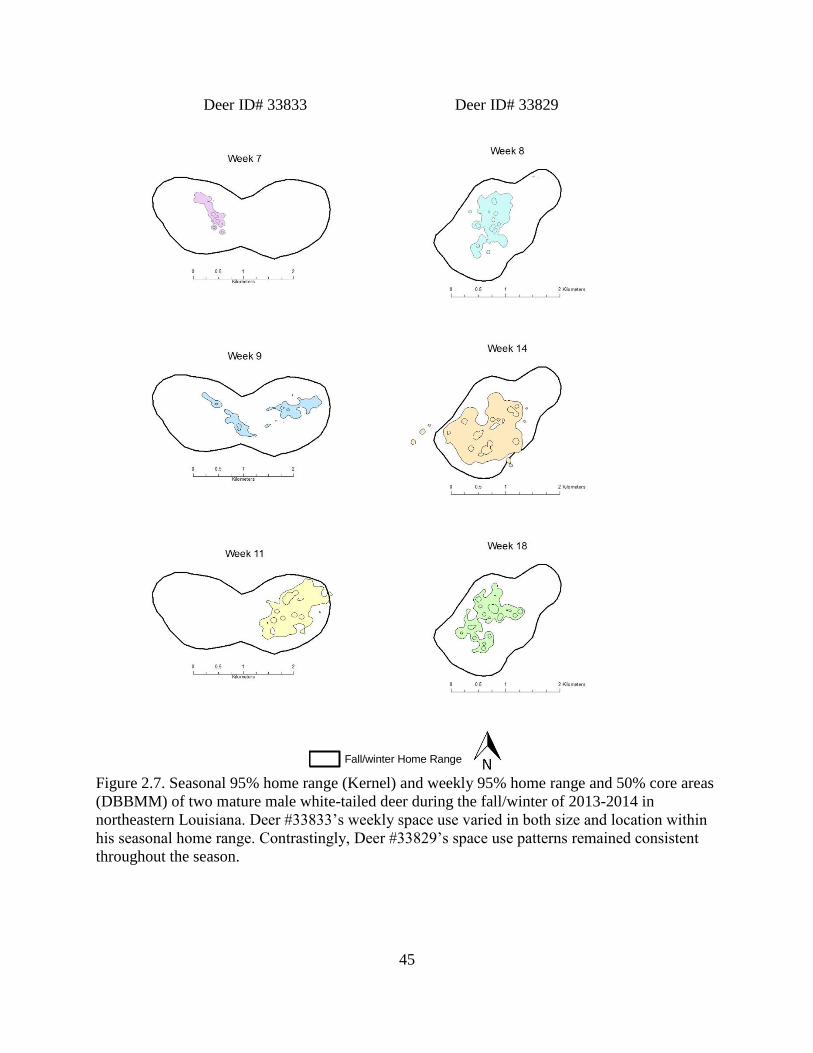
45

Deer ID# 33833 Deer ID# 33829

Figure 2.7. Seasonal 95% home range (Kernel) and weekly 95% home range and 50% core areas

(DBBMM) of two mature male white-tailed deer during the fall/winter of 2013-2014 in

northeastern Louisiana. Deer #33833’s weekly space use varied in both size and location within

his seasonal home range. Contrastingly, Deer #33829’s space use patterns remained consistent

throughout the season.

ÜFall/winter Home Range

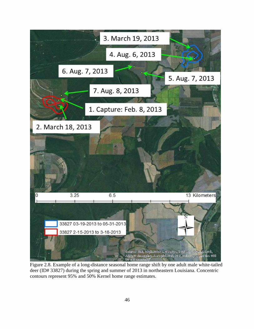
46

Figure 2.8. Example of a long-distance seasonal home range shift by one adult male white-tailed

deer (ID# 33827) during the spring and summer of 2013 in northeastern Louisiana. Concentric

contours represent 95% and 50% Kernel home range estimates.

47

Figure 2.9. Example of a non-breeding season excursion by an adult male white-tailed deer (ID#

35214) on March 28 and 29, 2014 in northeastern Louisiana. Green dots indicated locations of

the deer which show an excursion from his spring 95% Kernel home range (green polygon) into

his fall/winter home range (red polygon).

48

CHAPTER 3

FINE-SCALE MOVEMENTS OF ADULT MALE WHITE-TAILED DEER IN

NORTHEASTERN LOUISIANA DURING THE HUNTING SEASON

Simoneaux, T. N, B. S. Cohen, E. A. Cooney, R. M. Shuman, M. J. Chamberlain and K. V.

Miller. To be submitted to Journal of the Southeastern Association of Fish and Wildlife

Agencies.

49

ABSTRACT

An understanding of fine-scale movement patterns of adult male white-tailed deer

(Odocoileus virginianus) is critical to explaining population dynamics, competition and

predation interactions, gene flow, and disease and parasite spread of this demographic.

Relatively few studies have investigated movement ecology of mature male deer, although recent

trends in hunter-harvest selectivity have led to an increased representation of adult males in

many herds. Many factors influence deer movements, but individual deer should move at an

optimum rate to maximize individual health and fitness while minimizing high-risk encounters.

We obtained and analyzed GPS telemetry data from 24 adult male deer (≥ 2.5 years old) in

northeastern Louisiana to determine fine-scale movement patterns during the 2013-2014 and

2014-2015 hunting seasons. We calculated half-hour step lengths and used a generalized linear

mixed model to test the effects of habitat (agriculture, mature hardwoods, regenerating

hardwoods), age, breeding chronology (non-breeding, pre-rut, rut, post-rut), period (crepuscular,

day, night), and refugia from hunting (refuge or open access) on step length and used Akaike’s

information criterion (AIC) to test for model fit. We observed that interactions between period

and breeding chronology, along with the additive effect of refugia from hunting, were most

predictive of male movements. We conducted exploratory analyses to determine how each

variable influenced step length which indicated that movements were greater in agriculture and

mature hardwoods than regenerating hardwoods, and that males aged 5.5 years and older moved

less than males aged 3.5 and 4.5 years old. Likewise, movements were greatest during the rut and

least during the non-breeding period. Movements were greatest during crepuscular and night

hours, and least during the day. Male movements were greater in areas with open access to

hunting than in refuge areas. We observed that movements of mature males were greater during

50

crepuscular hours on the refuge and greater during day and night hours on open access areas,

suggesting that mature males were modifying movements to avoid hunter predation. Based on

the naïve prey theory, decreased disturbance from hunting may prevent deer from developing

antipredator behaviors, thereby facilitating successful harvest of these animals upon initiation of

hunting or deer movement outside of refuge boundaries.

INDEX WORDS: GPS, hunting pressure, Louisiana, movement, Odocoileus virginianus,

white-tailed deer

51

INTRODUCTION

Understanding animal movements is critical for explaining population dynamics,

competition and predation interactions, gene flow, and disease and parasite spread. Under the

optimality theory, animals should select behaviors which maximize individual fitness by

balancing increased movements to seek needed resources (e.g., food acquisition, mate finding)

with decreasing movements to avoid high-risk encounters such as predation (Reiss 1987).

Hunted animals encounter a perplexing situation as ephemeral predators (i.e., hunters) shift the

predation risk landscape both daily and seasonally. For many species, this process becomes more

dynamic as hunting season occurs during the peak of their breeding cycle. In hunted polygamous

species, males must balance the risk of natural and hunter-induced predation with increasing

movements to seek mates (Gude et al. 2006). In response, animals can shift the focus of their

movements to less risky areas (Burcham et al. 1999, Proffitt et al. 2009), times (Creel et al.

2008), or a combination which may differ among individuals (Bolnick et al. 2003).

The movement ecology of female and immature male white-tailed deer (Odocoileus

virginianus; hereafter deer) has been extensively characterized at varying spatial scales (Tester et

al. 1964, Beier and McCullough 1990, Kilpatrick et al. 2001, Brinkman et al. 2005, McCoy et al.

2005). However, recent trends in hunter-harvest selectivity have led to an increased

representation of adult males in many populations (Adams and Hamilton 2011, Adams and Ross

2014). Historic over-exploitation and under-representation in many deer herds has made studying

this demographic difficult. Consequently, little attention has been given to variables affecting

movement of adult male white-tailed deer during the breeding season, despite this time aligning

with hunting season.

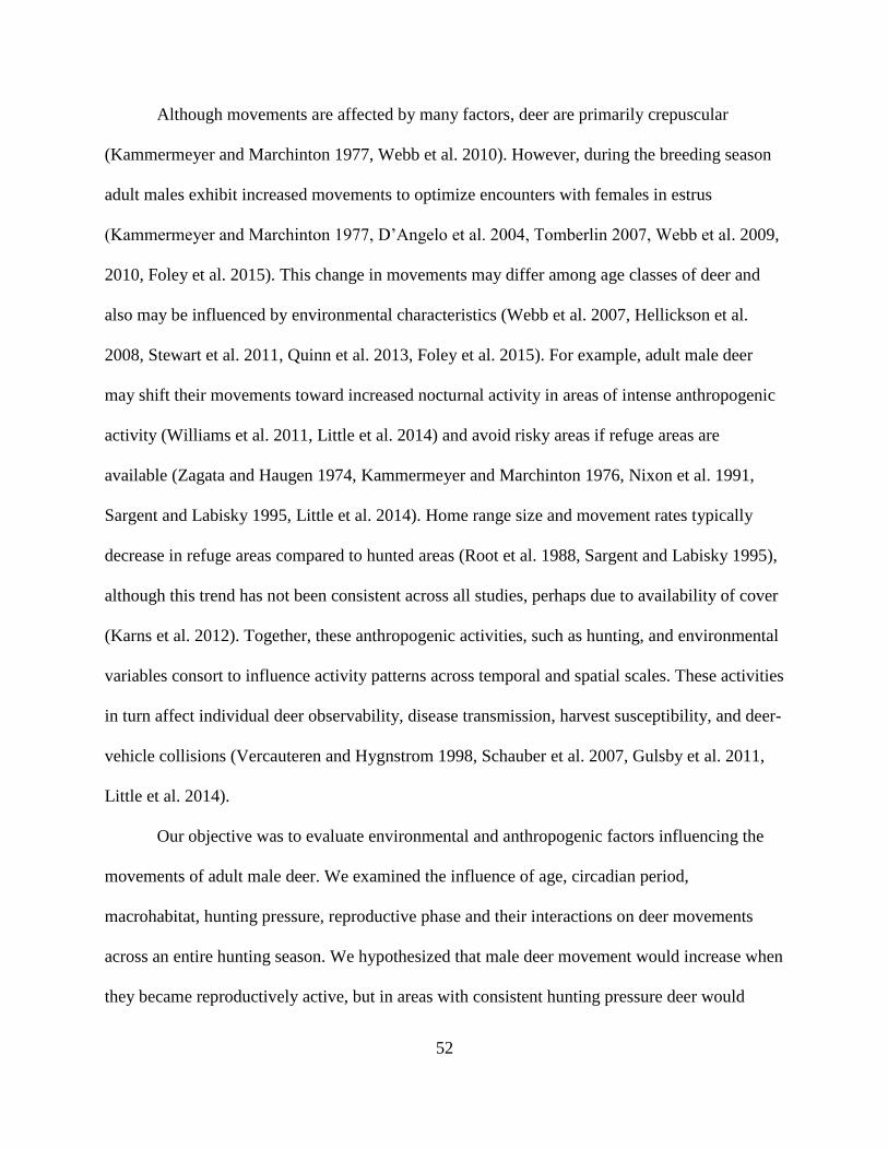
52

Although movements are affected by many factors, deer are primarily crepuscular

(Kammermeyer and Marchinton 1977, Webb et al. 2010). However, during the breeding season

adult males exhibit increased movements to optimize encounters with females in estrus

(Kammermeyer and Marchinton 1977, D’Angelo et al. 2004, Tomberlin 2007, Webb et al. 2009,

2010, Foley et al. 2015). This change in movements may differ among age classes of deer and

also may be influenced by environmental characteristics (Webb et al. 2007, Hellickson et al.

2008, Stewart et al. 2011, Quinn et al. 2013, Foley et al. 2015). For example, adult male deer

may shift their movements toward increased nocturnal activity in areas of intense anthropogenic

activity (Williams et al. 2011, Little et al. 2014) and avoid risky areas if refuge areas are

available (Zagata and Haugen 1974, Kammermeyer and Marchinton 1976, Nixon et al. 1991,

Sargent and Labisky 1995, Little et al. 2014). Home range size and movement rates typically

decrease in refuge areas compared to hunted areas (Root et al. 1988, Sargent and Labisky 1995),

although this trend has not been consistent across all studies, perhaps due to availability of cover

(Karns et al. 2012). Together, these anthropogenic activities, such as hunting, and environmental

variables consort to influence activity patterns across temporal and spatial scales. These activities

in turn affect individual deer observability, disease transmission, harvest susceptibility, and deer-

vehicle collisions (Vercauteren and Hygnstrom 1998, Schauber et al. 2007, Gulsby et al. 2011,

Little et al. 2014).

Our objective was to evaluate environmental and anthropogenic factors influencing the

movements of adult male deer. We examined the influence of age, circadian period,

macrohabitat, hunting pressure, reproductive phase and their interactions on deer movements

across an entire hunting season. We hypothesized that male deer movement would increase when

they became reproductively active, but in areas with consistent hunting pressure deer would

53

decrease crepuscular and daytime movements with the onset of hunting. In a refuge area where

hunter access was limited, we hypothesized that adult male circadian activity would not change

throughout the season.

STUDY AREA

We conducted research on the Tensas River National Wildlife Refuge (TRNWR) and

adjacent private lands located in northeastern Louisiana in the upper Tensas River Basin. The

30,750-ha refuge was established in 1980 and was once predominately agriculture after being

extensively logged. Since acquisition by the United States Fish and Wildlife Service, forests on

the refuge have grown into mature bottomland hardwood and swamps, and former agricultural

fields have been replanted in native hardwoods. The refuge was bordered almost entirely by

agriculture on all sides, making it an island of habitat for many species including deer and the

federally threatened Louisiana black bear (Ursus americanus luteolus).










established for carbon credits were distributed throughout the refuge. These hardwood plantings

were initiated between 1985 and 2009 and comprised about 6,110 ha of the refuge. During the

54

study, agricultural crops grown on private lands surrounding the refuge included corn (Zea

mays), cotton (Gossypium hirsutum), and soybeans (Glycine max) and rice (Oryza spp.).

Hunting pressure differed on the study area depending on whether deer were using public

or private lands, and whether deer on public lands were in areas open to hunting or in areas

generally closed to hunting. Although most of the study area was the TRNWR, deer we captured

spent time on both public and private lands. Deer hunting season on private land began with

archery hunting on October 1 and lasted until January 31 (123 days) with 20 days of primitive

weapon hunting and 65 days of modern firearms hunting. Although the general hunting season

on TRNWR began on October 1 (small game hunting), deer hunting began on November 2 and

consisted of 83 days of archery in 2013-14, or began on November 1 and consisted of 84 days of

archery during 2014-2015. Deer hunting season on TRNWR also included 7 days of modern

firearms hunting (2 days of youth only, 1 day antlerless only, 4 days of lottery hunts) and 2 days

of primitive weapons hunting. The Greenlea unit of the TRNWR was a 1066-ha area closed to

hunting with the exception of 3 days of staff-guided lottery deer hunts using modern firearms

on27 December 2013, 3 and 11 January 2014, 23 and 30December 2014, and 10 January 10

2015. Approximately 20 hunters were guided on each of these hunts.

METHODS

Data Collection

We captured adult (≥2.5 years) male deer during Jan.-March 2013 and 2014 using a

combination of drop nets (60’ x 60’ or 50’ x 50’), rocket nets (40’ or 60’) and free-range darting

with 3-ml Pneu-Dart transmitter darts (Pneu-Dart Inc., Williamsport, Pa and Daninject, Børkop,

Denmark). We anesthetized deer using a combination of ketamine (1.5 mg/kg)/xylazine (2.5

mg/kg) when caught under a net or Telazol (5 mg/kg)/xylazine (2.5 mg/kg) when darting. We

55

estimated age by tooth wear and replacement (Severinghaus 1949). We fit deer with either Lotek

7000mu GPS collars (Lotek Engineering, Ontario, Canada) or Followit Tellus® GPS collars

(Followit AB, Lindesberg, Sweden). Both types of collars allowed for remote data download via

Ultra High Frequency (UHF) signal. Following instrumentation, anesthesia was reversed using 3

ml of Tolazoline, half intravenously and half intramuscularly, and researchers remained with

animals until ambulatory. Capture and handling protocol was approved by the University of

Georgia Institutional Animal Care and Use Committee, permit #A2012 06-006-Y3-A2.

We programmed collars to collect 30-minute locations during the Louisiana state-wide

hunting season (Oct. 1 – Jan. 31). If a deer was captured in 2013 and survived to 2015, then

collars collected locations during both the 2013-2014 and 2014-2015 hunting seasons. We

monitored VHF signals once/week to determine activity mode of the collar (active, mortality,

low battery). We remotely downloaded data from collars at the end of each hunting season and

imported them to ArcGIS 10.2 (Environmental Systems Research Institute, Inc., Redlands, CA).

We censored data to eliminate non-fix and impossible locations.

Deer Movement

We calculated step lengths (the linear distance between consecutive points) for each 30

minute interval using the command “movement pathmetrics” in Geospatial Modeling

Environment (GME), version 0.7.3.0 (Beyer 2012). Hereafter, we refer to step length as

movement. In a mortality event, we calculated movement to the day before death. Two

movements were possible each hour.

Explanatory variables

We used National Oceanic and Atmospheric Administration sunrise and sunset tables to

divide days into 3 periods based on the amount of light available (Endler 1993). The crepuscular

56

period was the 6-hour period which included dawn (the hour bisected by sunrise and the hours

immediately before and after sunrise) and dusk (the hour bisected by sunset and the hours

immediately before and after sunset). The day period was the hours between dawn and dusk, and

night period was the hours between dusk and dawn.

To examine if macrohabitat features influenced the movement of deer, we created

broadly defined polygons for the study area. Because our study area was largely agriculture and

hardwoods, we confined our macrohabitat categories to agriculture (e.g. milo, corn, cotton,

soybeans, rice), regenerating hardwood (planted hardwoods), or mature hardwood. We assigned

each deer location as being present in agriculture, regenerating hardwood, or mature hardwood.

To examine the effect of reproductive phase on deer movement, we categorized each

movement based on the reproductive phase in which it occurred. Based on concurrent research at

our study area, the mode day of conception was December 20 and mode date of parturition was

July 8 (Figure 3.1). From these data, we divided the entire period of intensive monitoring, which

was centered on the hunting season, into 4 phases based on breeding phenology: non-breeding

(Oct. 1 - Nov. 25), pre-rut (Nov. 26 - Dec. 15), rut (Dec. 16 - Jan. 12), and post-rut (Jan. 13 - Jan.

31).

To examine the effect of age on deer movement, we assigned deer as 3.5, 4.5 or 5.5 and

older based on estimated age at time of capture. We conducted a preliminary analysis by

determining the mean movement of each deer per age and determining a mean and standard error

of movement for each age in our sample to determine if these ages could be combined into age

classes. Because our preliminary analysis suggested 3.5 and 4.5 year old deer had similar

average step lengths for our study, we combined ages into 2 classes: adult (3.5 and 4.5 years old)

57

or mature (≥ 5.5 years old; see results). If a deer was collared for 2 years, his age was

appropriately updated for the second hunting season (Table 3.1).

To examine the effect of hunting on deer movements, we categorized locations based on

hunting pressure. All visitors to TRNWR were required to check-in via self-clearing permits and

visitor numbers for each week of our study were provided to us by TRNWR staff. While the

specific activity for each visitor was not recorded, we assume most of this use was by hunters.

Because the summary data provided to us did not align with our predefined weeks, we calculated

a 3-week moving window average of visitor use as a surrogate for hunting pressure per week

(Figure 3.2). These data demonstrated that most land in the TRNWR received relatively

consistent hunting pressure. While we were unable to directly measure hunting pressure on

private lands, the primary use of those properties was deer hunting. Private lands and areas of

TRNWR open to hunting differed from the Greenlea Unit, which was only hunted for 3 days

annually and otherwise acted as a centrally located refuge in our study area (Figure 3.3).

Therefore, we assigned each deer location as occurring in open access (i.e., outside of Greenlea)

or refuge (i.e., inside of Greenlea).

Data Analysis

We first conducted exploratory analyses to determine how period, macrohabitat,

reproductive phase, age, and hunting pressure may influence movement. We categorized each

movement based on these aforementioned variables, then calculated a mean movement (i.e., step

length) for each individual deer based on each explanatory variable. This provided a sample

mean and standard error for movements to inform our modeling exercise. We conducted

statistical analyses using program R version 3.0.2 (R Core Team 2013).

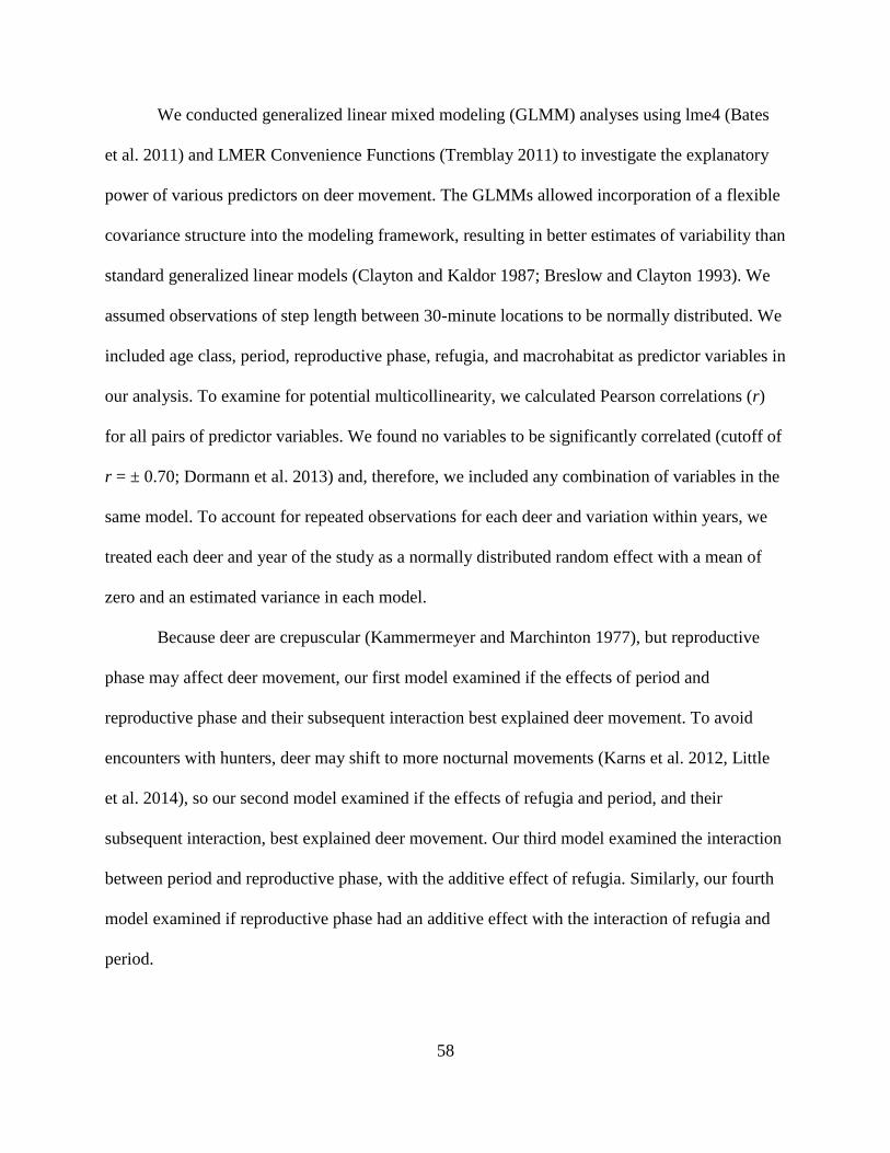
58

We conducted generalized linear mixed modeling (GLMM) analyses using lme4 (Bates

et al. 2011) and LMER Convenience Functions (Tremblay 2011) to investigate the explanatory

power of various predictors on deer movement. The GLMMs allowed incorporation of a flexible

covariance structure into the modeling framework, resulting in better estimates of variability than

standard generalized linear models (Clayton and Kaldor 1987; Breslow and Clayton 1993). We

assumed observations of step length between 30-minute locations to be normally distributed. We

included age class, period, reproductive phase, refugia, and macrohabitat as predictor variables in

our analysis. To examine for potential multicollinearity, we calculated Pearson correlations (r)

for all pairs of predictor variables. We found no variables to be significantly correlated (cutoff of

r = ± 0.70; Dormann et al. 2013) and, therefore, we included any combination of variables in the

same model. To account for repeated observations for each deer and variation within years, we

treated each deer and year of the study as a normally distributed random effect with a mean of

zero and an estimated variance in each model.

Because deer are crepuscular (Kammermeyer and Marchinton 1977), but reproductive

phase may affect deer movement, our first model examined if the effects of period and

reproductive phase and their subsequent interaction best explained deer movement. To avoid

encounters with hunters, deer may shift to more nocturnal movements (Karns et al. 2012, Little

et al. 2014), so our second model examined if the effects of refugia and period, and their

subsequent interaction, best explained deer movement. Our third model examined the interaction

between period and reproductive phase, with the additive effect of refugia. Similarly, our fourth

model examined if reproductive phase had an additive effect with the interaction of refugia and

period.

59

Because differing age classes of males may use different breeding strategies (Brown

1974, Webb et al. 2007, Hellickson et al. 2008, Foley et al. 2015), our fifth model examined if

the additive effect of age class and reproductive phase best predicted deer movement. Lastly,

because habitat may be one of the most influential variables on deer movement (Beier and

McCullough 1990, Vercauteren and Hygnstrom 1998, Lesage et al. 2000, Brinkman et al. 2005,

Long et al. 2005, Quinn et al. 2013) and likely has an additive effect with reproductive phase and

period, we examined if the combination of macrohabitat, reproductive phase, and period best

predicted deer movement. Because we believed a priori that all of these variables influenced

deer movement, we estimated effect sizes based on the additive effects of each of our fixed-

effect variables in a global model (Table 3.2).

While some debate remains about the appropriateness of information criteria approaches

with GLMMs (Vaida and Blanchard 2005), we conducted an exploratory analysis using Akaike's

information criterion (Akaike 1973) with small sample adjustment (AICc; Hurvich and Tsai,

1989) to determine which model best explained variation in movement. We compared our 7

predictive models with a global model consisting of all explanatory variables using deer and year

as random effects, and a null model consisting of an intercept estimate using deer and year as

random effects. We considered the model with the smallest AICc value to be the most plausible,

and models within a ∆AIC of less than 2 to be equally plausible. We calculated Akaike weights

(wi) to assess the empirical support for each model and select the most appropriate candidate

model. To examine the power of each model to predict movement, we also calculated marginal

R² (variability explained by only fixed-effects) and conditional R² (variability explained by both

fixed and random effects) in program R, package MuMIn (Nakagawa and Schielzeth 2013,

Johnson 2014). After selecting the most parsimonious mixed-effect model based on AICc, we

60

used the predict function (R Core Team 2013) to calculate expected movement values and 95%

confidence intervals based on the fixed effect variables.

We conducted a post hoc analysis to determine the percentage of time each deer spent on

the refuge, and to quantify potential differences in percent of time spent on the refuge between

harvested and non-harvested deer. We used a mean percentage of time on the refuge for each

deer to get a sample mean and standard error for harvested and non-harvested deer.

RESULTS

We captured 14 adult male deer in 2013, of which 14 survived to the 2013-2014 hunting

season and 8 survived to the 2014-2015 hunting season. We captured an additional 16 adult

males in 2014, of which 13 survived to the 2014-2015 hunting season. We lost data from 3 deer

because of collar malfunction, leaving us with 24 data-sets. We had 10 deer harvested during the

hunting season, resulting in 14-24 data-sets per week.

Movement was greatest during crepuscular hours (105 ± 5 m) and night (95 ± 5 m), and

least during the day (38 ± 3 m; Figure 3.4). Deer moved similarly in agriculture (92 ± 8 m) and

mature hardwoods (92 ± 6 m) but less in regenerating hardwood (69 ± 5 m; Figure 3.5).

Movements were greatest during the rut (120 ± 9 m) followed by pre-rut (89 ± 5 m), post-rut (90

± 10 m) and the non-breeding phase (63 ± 3 m; Figure 3.6). Adult males (82 ± 5 m) moved more

than mature males (69 ± 6 m; Figure 3.7). Lastly, deer tended to move more in areas with open

hunting (94 ± 7 m) than on the refuge area (75 ± 4 m; Figure 3.8).

Evidence from the global GLMM and model ranking suggested that reproductive phase

and period best predicted movements. The interaction between these 2 variables, and the additive

effect of hunting pressure, was the most parsimonious model and accounted for 52% of the

model weight. However, the model incorporating only reproductive phase and period had a

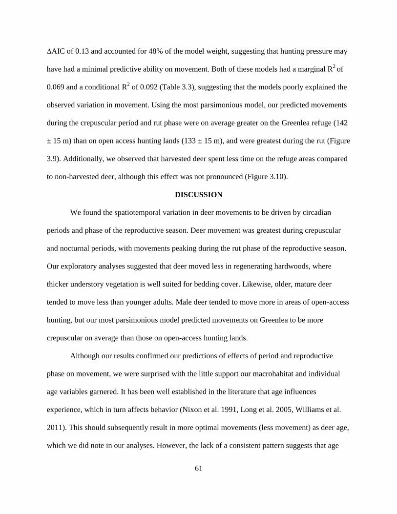
61

∆AIC of 0.13 and accounted for 48% of the model weight, suggesting that hunting pressure may

have had a minimal predictive ability on movement. Both of these models had a marginal R2

of

0.069 and a conditional R2 of 0.092 (Table 3.3), suggesting that the models poorly explained the

observed variation in movement. Using the most parsimonious model, our predicted movements

during the crepuscular period and rut phase were on average greater on the Greenlea refuge (142

± 15 m) than on open access hunting lands (133 ± 15 m), and were greatest during the rut (Figure

3.9). Additionally, we observed that harvested deer spent less time on the refuge areas compared

to non-harvested deer, although this effect was not pronounced (Figure 3.10).

DISCUSSION

We found the spatiotemporal variation in deer movements to be driven by circadian

periods and phase of the reproductive season. Deer movement was greatest during crepuscular

and nocturnal periods, with movements peaking during the rut phase of the reproductive season.

Our exploratory analyses suggested that deer moved less in regenerating hardwoods, where

thicker understory vegetation is well suited for bedding cover. Likewise, older, mature deer

tended to move less than younger adults. Male deer tended to move more in areas of open-access

hunting, but our most parsimonious model predicted movements on Greenlea to be more

crepuscular on average than those on open-access hunting lands.

Although our results confirmed our predictions of effects of period and reproductive

phase on movement, we were surprised with the little support our macrohabitat and individual

age variables garnered. It has been well established in the literature that age influences

experience, which in turn affects behavior (Nixon et al. 1991, Long et al. 2005, Williams et al.

2011). This should subsequently result in more optimal movements (less movement) as deer age,

which we did note in our analyses. However, the lack of a consistent pattern suggests that age

62

alone does not predict behavioral states, and experience may lead to individual specialization in

which manifested behaviors are more predicted based on past failures and successes than by age-

related experience (Bolnick et al. 2003). Alternatively, our observed similarities in movement

between age classes could be an artifact of our sample of deer being similarly aged. Had our

study encompassed immature deer as well as older, senescent deer, the impact of age may have

been more notable. The importance of habitat in behavioral processes is unquestionable, but the

scale of our macrohabitat variables may have been uninformative based on the fine-scale spatial

resolution of our data set.

Under the optimization theory, deer are predicted to increase movement rates in areas of

high predation risk as they look for safer areas (Reiss 1987). Supporting this theory, and similar

to others findings (Cleveland et al. 2012, Little et al. 2014), we noted that deer tended to move

more on average in open-access hunting lands compared to the Greenlea Unit. However, these

movements were largely during the night and day periods, suggesting deer in open access lands

may have moved less and spent time in safe patches during crepuscular periods. In many taxa,

increased movement rates result in lower survival and fitness (Biro et al. 2003), but for hunted

species such as deer, focusing these increased movements during nocturnal periods may offset

harvest-susceptibility. Deer in Greenlea were more crepuscular, further suggesting that open-

access hunting made deer more nocturnal. However, these patterns were not pronounced

suggesting that the degree of hunting pressure present on our study site may not have been

enough to warrant a major shift in behavior, similar to the findings of Karns et al. (2012).

Our regression analyses indicated that our models explained a relatively small amount of

movement variance, even when individual deer and years were included as random variables.

We offer that it is difficult to capture the diverse amount of environmental variables experienced

63

by an animal when measuring fine-scale movements. For example, weather patterns, local deer

density, and sex ratios may influence deer movements in conjunction (Beier and McCullough

1990, Sargent and Labisky 1995, Labisky and Fritzen 1998, D’Angelo et al. 2004, Webb et al.

2010, Williams et al. 2011), yet we could not quantify these parameters at an informative scale

for our data set. It is also possible that measurable variables are having less influence on deer

movement than previously suspected. For example, variations in behavior may be reflective of

individual specialization, making predictions to the general population difficult and tenuous

(Bolnick et al. 2003, Vander Zanden et al. 2010).

According to the naïve prey hypothesis, deer inhabiting a refuge would not develop

antipredator behaviors and, therefore, may be more susceptible to harvest should the deer move

outside of the refuge or upon initiation of hunting on the refuge (Martin 2014). Percentage of

time spent on the refuge between harvested and non-harvested deer was similar, suggesting that

although a deer may spend most of its time on a refuge, it is nearly as susceptible to harvest as

deer that spend most of their time in open access areas (Figure 3.10). This harvest susceptibility

occurred during times when deer ventured outside of the refuge and during the limited hunting

allowed on the refuge. This seems to support the naïve prey hypothesis, as it would be intuitive

to expect deer spending more time on the refuge to have higher survival. We offer that short,

intensive bursts of hunting may be equally effective as a liberal hunting framework for

harvesting deer, since deer in a refuge would not exhibit antipredator behavior typically

associated with greater predation risk.

MANAGEMENT IMPLICATIONS

Hunting pressure had relatively little effect on movement of adult males compared to

period and reproductive phase. The amount of escape cover available and degree of disturbance

64

influence response to hunting pressure (Karns et al. 2012). Most of our study area had dense

understory vegetation and most hunting pressure was from archery hunting. In areas with sparse

understory cover, a greater frequency of gun hunts, and/or higher hunter densities, the degree to

which hunting pressure influences movements would likely be different. Further research should

be conducted examining the impact of escape cover and the intensity of hunting pressure as it

relates to deer movement.

Although hunting pressure had a relatively small effect on movement compared to period

and reproductive phase, our results suggest that the naïve prey hypothesis comes into effect

regarding deer on a limited-hunting refuge. If the goal of a refuge is to protect deer to reach an

older age class, then the intensity of hunting without compromising that goal should be

considered. The size of the refuge should also be considered, as we reported that many deer spent

varying amounts of time on and off of the refuge. This suggests that deer on the Greenlea Unit

were still very susceptible to mortality despite the fact they spent most of their lives protected

from harvest. Additionally, if the goal of the refuge is to produce a quality hunting experience

with older age class of deer, then the intensity of hunting allowable before deer enact

antipredator behaviors should be examined.

65

LITERATURE CITED

Adams, K. and M. Ross. 2014. QDMA’s Whitetail Report 2014. Quality Deer Management

Association, Bogart, GA.


editor. Biology and Management of White-tailed Deer, CRC Press, Boca Raton, FL.

Akaike H. 1973. Information theory and an extension of the maximum likelihood principle.

Pages 267-281 in Petrov B. N. and F. Csaki, editors. Proceedings of the Second

International Symposium on Information Theory, Akademiai Kiado, Budapest, Hungary.

Bates D., M. Maechler, and Bolker B. M. 2011. lme4: Linear mixed-effects models using S4

classes version 0.999375-39. Available at http://CRAN.R-project.org/package5lme4.



Beyer, H. L. 2012. Geospatial Modelling Environment. Available at

http://www.spatialecology.com/gme.

Biro, P. A., J. R. Post, and E. A. Parkinson. 2003. From individuals to populations: prey fish

risk-taking mediates mortality in whole-system experiments. Ecology 84:2419-2431.

Bolnick, D. I., R. Svanback, J. A. Fordyce, L. H. Yang, J. M Davis, C. D. Hulsey, and M. L.

Forister. 2003. The ecology of individuals: incidence and implications of individual

specializations. American Naturalist 161:1-28.

Breslow N. E. and Clayton D. G. 1993. Approximate inference in generalized linear mixed

models. Journal of the American Statistical Association 88:9-25.

66

Brinkman, T. J., C. S. Deperno, J. A. Jenks, B. S. Haroldson, and R. G. Osborn. 2005. Movement

of female white-tailed deer: effects of climate and intensive row-crop agriculture. Journal

of Wildlife Management 69:1099-1111.


Geist and F. Walther, editors. The behaviour of ungulates and its relation to management.

International Union Conservation of Nature Publications 24, Morges, Switzerland. pp.

436-446.

Burcham, M., W. D. Edge, and C. L. Marcum. 1999. Elk use of private land refuges. Wildlife

Society Bulletin 27: 833-839.

Clayton D. and J. Kaldor. 1987. Empirical Bayes estimates of age-standardized relative risks for

use in disease mapping. Biometrics 43:871−681.

Cleveland, S. M., M. Hebblewhite, M. Thompson, and R. Henderson. 2012. Linking elk

movement and resource selection to hunting pressure in a heterogeneous landscape.

Wildlife Society Bulletin 36:658-668.

Creel, S., J. A. Winnie Jr., D. Christianson and S. Liley. 2008. Time and space in general models

of antipredator response: tests with wolves and elk. Animal Behaviour 76:1139-1146.

D'Angelo, G. J., C. E. Comer, J. C. Kilgo, C. D. Drennan, D. A. Osborn, and K. V. Miller. 2004.

Daily movements of female white-tailed deer relative to parturition and breeding.

Proceedings of the Southeastern Association of Fish and Wildlife Agencies 58:292-301.

Dormann C. F., J. Elith, S. Bacher, C.Buchmann, G. Carl, G. Carré, J. R. García Marquéz, B.

Gruber, B. Lafourcade, P. J. Leitão, et al. 2013. Collinearity: A review of methods to deal

with it and a simulation study evaluating their performance. Ecography 36:27–46.

67

Endler, J. A. 1993. The color of light in forests and its implications. Ecological Monographs

63:1-27.

Foley, A. M., R. W. DeYoung, D. G. Hewitt, M. W. Hellickson, K. L. Gee, D. B. Wester, M. A.

Lockwood, and K. V. Miller. 2015. Purposeful wanderings: mate-search strategies of

male white-tailed deer. Journal of Mammalogy: in press.

Gude, J. A., R. A. Garrott, J. J. Borkowski, and F. King. 2006. Prey risk allocation in a grazing

ecosystem. Ecological Applications 16:285-298.







Hurvich C. M., and C. L. Tsai. 1989. Regression and time series model selection in small

samples. Biometrika 76:297-307.

Johnson, P. C. D. 2014. Extension of Nakagawa & Schielzeth's R2

GLMM to random slopes

models. Methods in Ecology and Evolution 5:944-946.

Kammermeyer, K. E., and R. L. Marchinton. 1976. The dynamic aspects of deer populations

utilizing a refuge. Proceedings of the Southeastern Association of Game and Fish

Commissions 29:466-475.

Kammermeyer, K. E., and R. L. Marchinton. 1977. Seasonal change in circadian activity of

radio-monitored deer. Journal of Wildlife Management 41:315-317.

68

Karns, G. R., R. A. Lancia, C. S. DePerno, and M. C. Conner. 2012. Impact of hunting pressure

on adult male white-tailed deer behavior. Proceedings of the Southeastern Association of

Fish and Wildlife Agencies 66:120-125.



954.

Labisky, R. F., and D. E. Fritzen. 1998. Spatial mobility of breeding female white-tailed deer in a

low-density population. Journal of Wildlife Management 62:1329-1334.



78:1930-1940.






86:623-629.

Martin, C. W. 2014. Naïve prey exhibit reduced antipredator behavior and survivorship. PeerJ

2:e665; DOI 10.7717/peerj.665.

McCoy, J. E., D. G. Hewitt, and F. C. Bryant. 2005. Dispersal by yearling male white-tailed deer

and implications for management. Journal of Wildlife Management 69:366-376.

Nakagawa, S., and H. Schielzeth. 2013. A general and simple method for obtaining R^2 from

generalized linear mixed‐effects models. Methods in Ecology and Evolution 4:133-142.

69

Nixon, C. M., L. P. Hansen, P. A. Brewer, and J. E. Chelsvig. 1991. Ecology of white-tailed deer

in an intensively farmed region of Illinois. Wildlife Monographs 118:1-77.

Proffitt, K. M., J. L. Grigg, K. L. Hamlin, and R. A. Garrott. 2009. Contrasting effects of wolves

and human hunters on elk behavioral responses to predation risk. Journal of Wildlife




R Core Team. 2013. R: a language and environment for statistical computing. R foundation for

Statistical Computing, Vienna, Austria.

Reiss, M. J. 1987. Optimization theory in behavioural ecology. Journal of Biological Education

21:241-247.

Root, B. G., E. K. Fritzell, and N. F. Giessman. 1988. Effects of intensive hunting on white-

tailed deer movement. Wildlife Society Bulletin 16:145-151.

Sargent, R. A., and R. F. Labisky. 1995. Home range of male white-tailed deer in hunted and

non-hunted populations. Proceedings of the Southeastern Association of Fish and

Wildlife Agencies 49:389-398.



71:155-163.

Severinghaus, C. W. 1949. Tooth development and wear as criteria of age in white-tailed deer.


70


218. in D.G. Hewitt, editor. Biology and Management of White-tailed Deer. CRC Press,

Boca Raton, FL.





Tremblay, A. 2011. LMERConvenienceFunctions: A suite of functions to back-fit fixed effects

and forward-fit random effects, as well as other miscellaneous functions, Version 1.6.7.

http://CRAN.R-project.org/package5LMERConvenienceFunctions.

Vaida F., and S. Blanchard. 2005. Conditional Akaike information for mixed-effects models.

Biometrika 92:351-370.

Vander Zanden, H. B., K. A. Bjorndal, K. J. Reich, and A. B. Bolten. 2010. Individual specialists

in a generalist population: results from a long-term stable isotope series. Biology Letters

6:711-714.




white-tailed deer as influenced by home range and movements. Journal of Wildlife





71



Mammalogy 90:1210-1217.

Williams, D. M., A. C. Dechen Quinn, and W. F. Porter. 2011. Landscape effects on scales of

movement by white-tailed deer in an agricultural–forest matrix. Landscape Ecology

27:45-57.

Zagata, M. D. and A. O. Haugen. 1973. Pilot Knob State Park: a winter deer haven. Iowa State

Journal of Research 47:119-217.

72

Table 3.1. Age distribution of collared adult male white-tailed deer included in the study. Data

collection occurred during the 2013-2014 and 2014-2015 hunting seasons in northeastern

Louisiana.

Age 2013-2014 2014-2015

3.5 7 5

4.5 1 8

5.5+ 6 4

Table 3.2. Mixed models used to evaluate relative importance of age class, period, macrohabitat,

hunting pressure and reproductive phase on the movement of adult male white-tailed deer during

the 2013-2014 and 2014-2015 hunting seasons in northeastern Louisiana.

No. Model Name Hypothesis Models

1 Global All main effects at deer level will

change response parameter.

y = Age Class + Refugia

+ Period + Macrohabitat

+ Reproductive Phase +

Rja

2 Diel Movements

and Breeding

Response is dependent on the

interaction effect of breeding

chronology and time of day

y = Reproductive Phase

* Period + Rj

3 Predation

Avoidance


interaction of refugia and diel

movements.

y = Refugia * Period +

Rj

4

Diel Movements

and Breeding with

pressure



movements, with an additive effect of

refugia.

y = Reproductive Phase

* Period + Refugia + Rj

5

Predation

Avoidance with

Breeding



movements with an additive effect

from breeding chronology.

y = Refugia * Period +

Reproductive Phase + Rj

6

Age-related

Breeding

Strategies


additive effect of age class and

breeding chronology.

y = Age Class +

Reproductive Phase + Rj

7

Habitat and

Exploratory

Analysis


additive effects of habitat, breeding

chronology, and time of day.

y = Macrohabitat +

Reproductive Phase +

Period + Rj

8 Random Effects Response is dependent on random

variables deer and year. y = Rj

aRj = Random variables of individual and year of study.

73

Table 3.3. Akaike information criterion with small sample bias adjustment (AICc), number of

parameters (K), ∆AICc, Akaike weights (w) for candidate models (i) relating to variables

influencing step length of adult male white-tailed deer in northeastern Louisiana during the

2013-2014 and 2014-2015 hunting seasons.

Candidate Model Model

No. K AICc ∆AICc wi

Conditional

R2

Marginal

R2

Diel Movements and

Breeding with pressure 4 16 1926219 0 0.52 0.092 0.069

Diel Movements and

Breeding 2 15 1926219 0.13 0.48 0.092 0.069

Predation Avoidance

with Breeding 5 12 1926435 215.8 0 0.091 0.068

Global 1 13 1926444 224.85 0 0.093 0.069

Habitat and Exploratory

Analysis 7 11 1926452 232.74 0 0.091 0.068

Predation Avoidance 3 9 1929821 3601.64 0 0.068 0.046

Age-related Breeding

Strategies 6 8 1933738 7518.67 0 0.047 0.025

Random Effects 8 4 1937289 11069.24 0 0.022 0.000

74

Figure 3.1. Number of conceptions per week from October 1 to January 31 of 2013-2014 and

2014-2015. Based on these data, we assigned a reproductive phase to each day of our study. We

used this to calculate the effect of reproductive phase on the movements of 24 adult white-tailed

deer in northeastern Louisiana during the 2013-2014 and 2014-2015 hunting seasons.

Figure 3.2. Number of visitors based on self-clearing permits during the 2013-2014 and 2014-

2015 hunting seasons fitted to our predefined weeks using a 3 week moving window analysis.

75

Figure 3.3. Map of the study area including the Tensas River National Wildlife Refuge (open-

access hunting), Greenlea unit (refuge), and adjacent private lands in northeastern Louisiana.

Locations (30-min) were obtained for 24 adult male white-tailed deer that inhabited the area and

movements were compared for movement within and outside the Greenlea refuge.

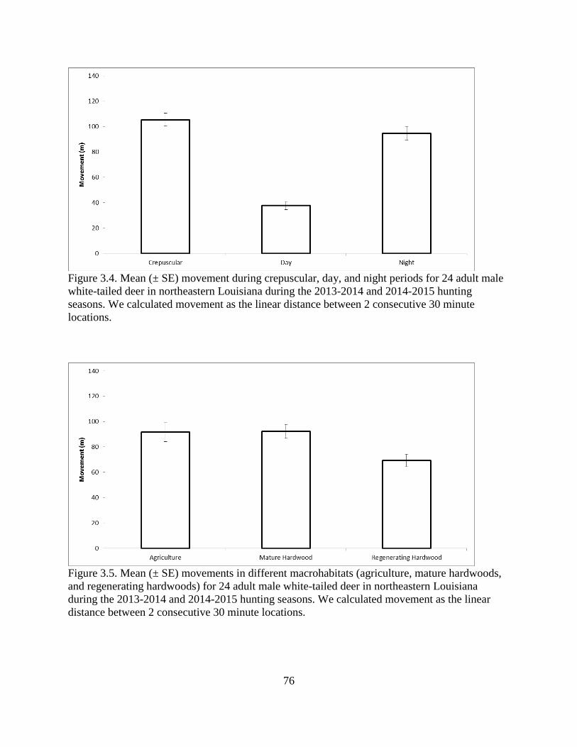
76

Figure 3.4. Mean (± SE) movement during crepuscular, day, and night periods for 24 adult male



locations.

Figure 3.5. Mean (± SE) movements in different macrohabitats (agriculture, mature hardwoods,

and regenerating hardwoods) for 24 adult male white-tailed deer in northeastern Louisiana

during the 2013-2014 and 2014-2015 hunting seasons. We calculated movement as the linear

distance between 2 consecutive 30 minute locations.

77

Figure 3.6. Mean (± SE) movements across the reproductive phase (non-breeding, pre-rut, rut,

and post rut sub-periods) for 24 adult male white-tailed deer in northeastern Louisiana during the

2013-2014 and 2014-2015 hunting seasons. We calculated movement as the linear distance

between 2 consecutive 30 minute locations.

Figure 3.7. Mean (± SE) movements of different aged male white-tailed deer in northeastern

Louisiana during the 2013-2014 and 2014-2015 hunting seasons. We categorized deer as adult

(3.5 and 4.5 years old) and mature (5.5 years and older). We calculated movement as the linear

distance between 2 consecutive 30 minute locations.

78

Figure 3.8. Mean (± SE) movements in refuge and open-access hunting areas for adult male



locations.

Figure 3.9. Movements of adult male deer during crepuscular, day, and night periods in open

access and refuge areas in northeastern Louisiana during the non-breeding, pre-rut, rut, and post-

rut reproductive phases in 2013-2014 and 2014-2015 hunting seasons as predicted by our most

parsimonious model.

79

Figure 3.10. Mean (±SE) percentage of time spent on refuge area (Greenlea) for harvested

(n=13) and un-harvested (n=11) adult male white-tailed deer in northeastern Louisiana during

the 2013-2014 and 2014-2015 hunting seasons.

Documents

SPACE-USE AND MOVEMENTS OF ADULT MALE WHITE …