AD-A247 463 "1I 10t it1l~ l t 111lll l NH tiP~lrllt tII

NAVAL POSTGRADUATE SCHOOLMonterey, California

OIL

Sp STAfte J

DTiC101A71 2 1992E

THESIS

FULL POSE AND PARTIAL POSE CALIBRATIONOF A SIX DEGREE OF FREEDOM

ROBOT MANIPULATOR ARM

by

Scott A. Potter

September 1991

Thesis Advisor: Morris R. Driels

Approved for public release; distribution is unlimited.

92-06410

, U1jIIIIq!!Iv ' I~

UnclassifiedSECURITY CLASSIFICATION OF THIS PAGE

REPORT DOCUMENTATION PAGEIa. REPORT SECURITY CLASSIFICATION lb. RESTRICTIVE MARKINGS

Unclassified2a. SECURITY CLASSIFICATION AUTHORITY 3. DISTRIBUTION. AVAILABILITY OF RLPORT

Approved for public relcase: distribution i unlimited.

4. PERFORMING ORGANIZATION REPORT NUMBER(S) 5. MONITORING ORGANIZATION REPORT NUMBER(S)

6a. NAME OF PERFORMING ORGANIZATION 6b. OFFICE SYMBOl 7a. NAME OF MONITORING ORGANIZATONNaval Postgraduate SchoolI (If ApplCalci Naval Postgraduate School

6c. ADDRESS (city, state and ZIP code) 7b. ADDRESS (city, state, and ZIP codejMonterey, CA 93943-5000 Monterey, CA 93943-5000

8a. NAME OF FUNDING/SPONSORING 6b. OFFICE SYMBOL 9. PROCUREMEN-I INSTRUMENT IDENTIF ICATO)N NUMBIkORGANIZATION (If Applicable)

8c. ADDRESS (city, state, and ZIP code) 10. SOURCE OF FUNDING NUMBERS

PROGRAM PROJEC'I TASK WORK UNITELEMENT NO. NO. NO. ACCESSION NO.

11. TITLE (Includ .ecurit. Ctacs:fl, ,ztaFULL POSE AND PARTIAL POSE CALIBRATION OF A SIX DEGREE OF FREEDOM ROBOT MANIPULATOR ARM

12. PERSONAL AUTHOR(S)

Potter, Scott Alton13a. TYPE OF REPORT 13b. TIME CE 14. DATE OFRPM (year, mont day.j 15. .PAGF COUNT

Master's Thesis FROM 1/91 TO 9/91 September 1991 13116. SUPPLEMENTARY NOTATION

The views expressed in this thesis are those of the author and do not reflect the official polic) or position of the Department ofDefense or the U.S. Government.

17. COSATI CODES lb. SUBJI'T TERMS (continue on reverse if nccessary and id'nttf% bi bh,'k numb,'r

FIELD GROUP SUBGROUP Robot Manipulator Calibration

19. ABSTRACT (Continue on reverse if necessary and idntif% by block number)

A six degree of freedom robot manipulator arm, a PUMA 560, is calibrated using full pose and partial pose methods inorder to improve the accuracy of the manipulator arm. The theory applicable to modeling of mechanisms is introduced. Athirty parameter kinematic model is developed for use in the full pose calibration method and a twenty-six parameterkinematic model is developed for the partial pose calibration. A simulation study is performed to determine the applicabilityand feasibility of each model. Experimental pose measurements are performed using each method to obtain data with whichto perform an actual calibration of the manipulator and compare with the predicted results. The effects of noise in eachmeasurement system employed and in the manipulator's joint position encoders are discussed. The measurement systemsemployed are examined in detail and a comparison between the two is performed.

The measured kinematic parameters of each model are presented as results.

20. DISTRIBUTIONAVAILABILITY OF ABSTRACT 21. ABSTRACT SECURITY CLASSIFICATION

X UNCLASSIFIED/UNLIMITED __ SAME AS RFPr , DTIC USERS Unclassified

M. NAME OF RESPONSIBLE INDIVIDUAL 0T P (Include Area Code) 22Yx OFFICE SYMBOLProfessor Morris R. Driels (408) 646-3383 69Dr

DD FORM 1473, b4 MAR 83 APR edition ma, be used until exhausted SIECURIT CLASSIIICATION OF TIllS PAii

All other editions are obsolele Unclassified

Approved for public release; distribution is unlimited.

Full Pose and Partial Pose Calibrationof a Six Degree of Freedom

Robot Manipulator Arm

by

Scott Alton PotterLieutenant, United States Navy

B.E., Vanderbilt University, 1986

Submitted in partial fulfillment of therequirements for the degree of

MASTER OF SCIENCE IN MECHANICALENGINEERING

from the

NAVAL POSTGRADUATE SCHOOLSeptember 1991

Author: _'1 _ _ _ _------Scott A. Potter

Approved by: : _ _ _ _ _ _ _ _ _ _Morris Driels, Thesis Advisor

Anthony J. l- aley, Chairmg /Department of Mechanical Engir96ring

ABSTRACT

A six degree of freedom robot manipulator arm, a PUMA 560, is calibrated using full

pose and partial pose methods in order to improve thc accuracy of the manipulator arm.

The theory applicable to modeling of mechanisms is introduced. A thirty parameter

kinematic model is developed for use in the full pose calibration method and a twenty-six

parameter kinematic model is developed for the partial pose calibration. A simulation study

is performed to determine the applicability and feasibility of each model. Experimental

pose measurements are performed using each method to obtain data N% Ith which to perform

an actual calibration of the manipulator and compare with the predicted results. The effects

of noise in each measurement system employed and in the manipulator's joint position

encoders are discussed. The measurement systems employed arc examined in detail and a

comparison between the two is performed.

The measured kinematic parameters of each model are presented as results.

Acoesslon For

J).' , tQ

iiIiJC I; uli;:;; :odes... D I s. L S v, 3 c a l

TABLE OF CONTENTS

I. INTRODUCTION ............................................................................. I

II. T H E O RY ........................................................................................ 5

A. MODELING .......................................................................... 5

1. Homogeneous Transformations ............................................. 5

2. Application of Basic Homogeneous Transformations to Simple Kinematic

Mechanisms ................................................................... 11

3. Links, Joints, and Assignment of Coordinate Frames ................... 13

4. The Denavit-Hartenburg Transformation ................................. 17

5. The Modified Denavit-Hartenburg Transformation ....................... 19

6. The Euler Transformation .................................................... 20

7. Application to the PUMA .................................................... 21

B. IDENTIFICATION METHODOLOGY ......................................... 27

1. Introduction ................................................................... 27

2. The IMSL routine ZXSSQ .................................................. 29

3. Application to the Calibration Process .................................... 33

III. FULL POSE CALIBRATION ............................................................. 35

A. THEORY .............................................................................. 35

1. Introduction ................................................................... 35

2. Full Model of the PUMA, World Coordinate Frame, and Coordinate

Measuring Machine ............................................................. 37

B. SIMULATION ........................................................................ 39

1. The Suite of Programs Used and the Strategy Involved ................... 39

a. The program JOINT .................................................. 41

iv

b. The program POSE .................................................... 41

C. ThL: piogram ID ........................................................ 43

d. The program VERIFY ................................................. 45

C. EXPERIMENTATION ............................................................... 46

1. The Tooling Ball End Effector ............................................. 46

2. The Coordinate Measuring Machine and World Coordinate Frame ...... 47

a. Construction ........................................................... 47

b. Data Acquisition Using the Coordinate Measuring Machine ........ 51

c. Identification of Actual Kinematic Parameters ........................ 53

IV. PARTIAL POSE CALIBRATION ...................................................... 55

A. THEORY ............................................................................... 55

1. Introduction ................................................................... 55

2. Full Model of the Puma and the Linear Slide .............................. 57

B. SIMULATION ..................................................................... 59

1. The Suite of Programs Used and the Strategy Involved ................ 59

a. The program LINSC .................................................. 60

b. The program ID6_LINSC ........................................... 61

C. EXPERIMENTATION ............................................................... 63

1. The Coordinate Measuring Machine as a Linear Slide .................... 63

a. Construction ........................................................... 63

b. Data Acquisition Using the Linear Slide .............................. 64

c. Identification of Actual Kinematic Parameters ..................... 65

V. DISCUSSION OF RESULTS ............................................................. 67

A. GENERAL OBSERVATIONS ...................................................... 67

B. COMPARATIVE OBSERVATIONS ........................................... 69

V

VI. CONCLUSIONS ............................................................. 75

APPENDIX A ..................................................................... 76

APPENDIX B ..................................................................... 78

APPENDIX C ..................................................................... 83

APPENDIX D ..................................................................... 86

APPENDIXE ................. I.................................................... 91

APPENDIX F ..................................................................... 98

APPENDIX G ................................................................... 102

APPENDIX H .................................................................. 109lo

APPENDIX I .................................................................... 11II

LIST OF REFERENCES .......................................................... 118

INITIAL DISTRIBUTION LIST................................................... 120

vi

LIST OF FIGURES

Figure 1. A Homogeneous Transformation ................................................ 5

Figure 2. Position of Point A with respect to a World Coordinate Frame ................. 6

Figure 3. Translation of a Point in Space from Point A to Point B ...................... 8

Figure 4. Rotation of Point A 90 Degrees about the Z-axis. Rot(z.90) ................ 10

Figure 5. A Multiple Translation and Rotation Transformation of Point A .............. 11

Figure 6. A Two-Link Kinematic Mechanism ............................................... 12

Figure 7. The Length, a, and Twist, a, of a Link .......................................... 13

Figure 8. Illustration of Link Dimensions a and a ........................................ 14

Figure 9. Link Parameters 0, d, a, and a ................................................... 15

Figure 10. Revolute Joint ....................................................................... 16

Figure 11. Prismatic Joint ..................................................................... 17

Figure 12. Homogeneous Transformation Loop ......................................... 22

Figure 13. Links and Joints of the PUMA 560 Robot Manipulator Arm ................. 23

Figure 14. PUMA Frame Allocation ....................................................... 24

Figure 15. Generic Function in the x-y Plane ............................................... 27

Figure 16. Example of Two-Variable Function G(x,y) ................................... 28

Figure 17. Flowchart of the Operation of ZXSSQ ........................................ 30

Figure 18. Determination of the Center of a Ball in Space ............................... 31

Figure 19. Base Transformations ............................................................ 36

Figure 20. Full Pose Calibration Apparatus: PUMA, World Coordinate Frame and

Coordinate Measuring Machine ................................................................ 38

Figure 21. Flowchart for Full Pose Simulation ............................................ 40

Figure 22. Tooling Ball End Effector .......................................................... 47

vii

Figure 23. Coordinate Measuring Machine ................................................ 48

Figure 24. The Full Pose World Coordinate Frame Cube ................................... 49

Figure 25. Linear Slide Transformations .................................................. 56

Figure 26. Partial Pose Calibration Apparatus: PUMA and Linear Slide ................. 57

Figure 27. Flowchart for Partial Pose Simulation ............................................ 59

Figure 28. Coordinate Measuring Machine as Linear Slide ................................. 64

Figure 29. The PUMA 560 in Lefty, Elbow Down Configuration ....................... 68

viii

LIST OF TABLES

Table 1. Nominal Kinematic Parameters for the PUMA 560 ............................ 26

Table 2. Nominal Kinematic Parameters for the Full Pose Calibration .................... 39

Table 3. Full Pose Identified Parameters ................................................... 54

Table 4. Nominal Kinematic Parameters for the Partial Pose Calibration ................ 58

Table 5. Partial Pose Identified Parameters ................................................. 66

Table 6. Comparison Between Full and Partial Pose Identified Kinematic Parameters. 70

ix

I. INTRODUCTION

In the calibration of a manipulator the desired result is to significantly improve the

manipulator's accuracy. Accuracy is defined as the ability of a robot to move to a

commanded pose defined in the manipulator's working volume IRef. 1]. Stated simply.

how accurately can the origin of a coordinate frame and the orientation of the coordinate

axes attached to the end effector of the manipulator arm, to be termed achieving a certain

pose, be positioned in relation to a commanded point and orientation in the manipulator's

working volume? Present experimentation shows that manipulators have an accuracy of

about 10.0 mm [Ref. 21.

Another indication of a manipulator's ability to achieve a pose is it's repeatability.

Repeatability is the ability of a manipulator to return to a previously achieved pose [Rcf. 3].

To illustrate repeatability, consider the following. A manipulator arm's end effector,

termed the tool. is moved to a certain position and orientation in the working volume. After

the position of each joint angle of the manipulator is recorded, the tool's position and

orientation is altered. The manipulator is commanded to assume the previously recorded

joint angles. Examination will reveal that the tool's position and orientation will differ from

the originally learned pose. This is the error in repeatability of a manipulator arm. Present

experimentation shows that manipulators have an repeatability of around 0.3 mm [Ref. 4].

To summarize, the fundamental difference between accuracy and repeatability is that

repeatability is the ability of the manipulator to return to a previously achieved pose and

accuracy is the ability of the manipulator to move to a pose that is specified in the working

volume and that may have never been previously reached. It is apparent that a more

accurate manipulator is desired over a more repeatable manipulator. The accurate

manipulator's working volume is unconstrained while the repeatable manipulator does not

I

have a working volume, only discrete positions which must be taught to the manipulator.

Correspondingly, the objective of the calibration process is to improve the accuracy of the

manipulator.

In order to understand how a calibration is performed on a manipulator one must

understand how a commanded pose would be achieved by any manipulator. When a

specific position and orientation is commanded to the manipulator, it must be specified

relative to a world coordinate frame defined by the user. To the manipulator this defined

world coordinate frame is, as described, the center of the universe. By means of several

mathematical operations the coordinate frame originally attached to the world coordinate

frame is moved from the world coordinate frame to the manipulator' base and through each

arm of the manipulator until it reaches the tool. This implies a knowledge of a mathematical

model of the manipulator which includes a world coordinate frame.

As it is prohibitively expensive to manufacture and assemble each manipulator to the

exact specifications required for desired accuracy, every manipulator built has a unique

geometry. Since each manipulator has this unique geometry, each will have a unique

mathematical model. The calibration process will identify the kinematic parameters

embedded within the manipulator in order that the individual mathematical model will

accurately represent the physical manipulator.

In the calibration process, several sequential steps enable the precise kinematic

parameters of the manipulator to be identified, leading to improved accuracy. These steps

are described as follows [Ref. 5]:

1. A kinematic model of the manipulator and calibration process is developed. The

resulting model is used to define a pose error quantity based on a nominal kinematic

parameter set, an unknown parameter set representing the true geometry of the manipulator

and a set of joint angles. The nominal kinematics would be supplied by the manufacturer of

2

the manipulator, while the unknown, actual parameter set will be identified in the

calibration process.

2. Experimental measurements of the robot pose, which could be either full pose

or partial pose. are taken in order to obtain data which correspond to the actual kinematic

parameters of the manipulator.

3. The actual kinematic parameters are identified by systematically changing the

nominal parameter set so as to reduce the error quantity defined in the modeling phase.

This is performed as a multidimensional optimization search in which the identified

kinematic parameters are changed in order to reduce an error function to a minimum

amount.

4. The final step involves incorporating the identified parameters into the actual

controlling software of the manipulator.

Once the calibration process is complete the next step is to implement the identified

kinematic parameters into the operation of the manipulator arm. In an operational setting

the required position and orientation of the manipulator arm's end effector would be input

to a controlling software program. This control program would perform an inverse

kinematic solution through the mathematical model of the manipulator encoded within the

control scheme, calculating the required joint angles to position and orient the end effector

as dictated by the operator.

This work addresses the issue of developing the kinematic model which represents

the PUMA manipulator arm and gathering the experimental data used in the calibration

process. Two methods will be described in this thesis: a full pose calibration process and a

partial pose calibration process.

The full pose calibration process will provide the benchmark calibration since the full

pose of the end effector will be measured in each observation.

3

Once the benchmark kinematic parameters are identified the second method of

calibration, the partial pose calibration wily be performed. The resuhling kinematic modcl

produced by this calibration will be contrasted with the values identified in the benchmark.

4

I1. THEORY

A. MODELING

The theory presented and several of the diagrams in this chapter follows closely that

presented by Paul [Ref. 6] in Chapters I through III. Also. several diagrams and

explanations in this chapter arc based on readings from Mooring. Roth. and Driels [Rcf.

71.

1. Homogeneous Transformations

The most basic premise on which the calibration process is associated is the

movement of a set of coordinate axes from one position and orientation in space to another

position and orientation, as illustrated in Figure 1. In Figure 1, the coordinate axes at point

A arc transformed, via translations and rotations, to point B.

Xl

k~y2

Sz2

Figure 1. A Homogeneous Transformation

In addition to the translation of the origin of the coordinate axes from one

position in spaccr O n th i,:r, i, ching, in 0A. oricntaion of thc coorjinie axes. ThL

process of the movement of the coordinate axes is known as a homogeneous

transformation. This homogeneous transformation is accomplished by a series of

translational transformations and rotational transformations.

The first type of transformation is the translational transformation. Given a

point in space, A, illustrated in Figure 2, the point's position is fixed and known relative to

a fixed, three axis coordinate frame, defined as the world coordinate frame, by means of

the following vector. u:

x

u=Yz

ZZ

Fir 2( )

y

U

Figure 2. Position of Point A with respect to a World Coordinate Frame

The matrix element w is any non-zero scale factor. In the applications reported

in this thesis w will be set equal to unity, producing the following vector:

6

x

(2)

The transformation from point A to point B, illustrated in Figure 3. requires the

transformation matrix H 1:

100a

H = Trans(x.y.z) = 01 h00 10001o (3)

The translation from point A to point B is represented h\ the \ cCtr v:

v = aI+hj+ck (4)

The transformed vector is the product of the transformation matrix. H. and the

original position vector, U.

v= H U

lOOa -x-OlOb yO01c z-0001 -1 (5)

The translation is to be interpreted as the summation of the vectors u and v.

This is illustrated in Figure 3 and described in equation form by equation (6).

7

y

II

Bz

Figure 3. Translation of a Point in Space from Point A to Point B

U+ '= _ + bj+cA (6)

The second type of transformation is the rotational transformation. Given the

fixed coordinate frame of the previously discussed translational transformation the

transformation corresponding to a rotation, 0, about the x-axis is:

1 0 0 0

Rot(xO) 0 cos(O) -sin(O) 0

0 sin(0) cos(O) 0

0 0 0 1 (7)

The transformation corresponding to a rotation, 0, about the y-axis is:

8

cos(O) 0 sin(O) 0

Rot ).0) 1 0 o

-sin(O) 0 cos(0) 0

0 0 0 1 (8)

The transformation corresponding to a rotation, 0. about the z-axis is:

cos(0) -sin(0) 0 0

sin(0) cos(0) 0 0Rot(z,0) =0 0 1 0

0 0 0 (

As an illustration of a rotational transformation consider the following. Given

another point in space, A. illustrated in Figure 4. if it was desired to rotate the point around

the z-axis by 90 degrees the Rot(z) matrix above would be used. The value for 0, 90

degrees, would be entered into the matrix, producing:

0-100Rot(z,90") = 1 0 0 0

0010-0001- (10)

This matrix would multiply the vector representing the original position of point

A:

=Y

.1_ (11)

producing the new position vector, v, of the point A.

0-100- -1 000 Y',0o010 z'

_0 001- -1- (12)

9

y

X

Figure 4. Rotation of Point A 90 Degrees about the Z-axis. Rot(z,90)

Translational and rotational transformations are performed right to left as they

are read, for example:

1 0 0 a 0 0 1 0 0-1 0 0

Trans(a,b,c)Rot(y,90)Rot(z,90) = 1 0 b 0 1 0 0 1 0 0 000 1 c -100 0 00 1 00 0 0 1 0 0 0 1 0 0 0 1 (13)

The transformation illustrated in Figure 5 is a a rotation of 90 degrees about the

z-axis, a rotation of 90 degrees about the y-axis, a translation of 'a' mm in the x direction,

of 'b' mm in the y direction, and of 'c' mm in the z direction.

10

Z

AY

* ~ //Ll

X

Figure 5. A Multiple Translation and Rotation Transformation of Point A

It is clear that an infinite number of translations or rotations are permitted. Each

transformation is simply represented b) another matrix multiplication operatio~n.

2. Application of Basic Homogeneous Transformations to Simple

Kinematic Mechanisms

Armed with the knowleIdge of homogeneous translations and rotations. a

genera. two link kinematic mechanism will be analyzed. When homogeneous

transformations are applied to the linkage shown in Figure 6. equations (3) and (9) will be

utilized to move coordinate frame 1, located at point 1, to coordinate frame 2, located at

point 2, by specifying the multiple transformation:

A = Trans(d ,0,0) Rot(z,01) Trans(d 2,0,0) (14)

11y

The product of the three matrix multiplications, a frame to frame homogeneous

transformation, is known as an A matrix. Referring to Figure 6, the coordinate frame at

point I has been assigned such that the x-axis lies along the centerline of link 1. As

illustrated in equation (14), the homogeneous transformation moves the coordinate frame

along the x-axis a distance d1, rotates the frame about the z-axis O1 degrees, and then

translates the coordinate frame a distance d2 along the newly rotated x-axis.

2, 2

y 1 ,

212

Figure 6. A Two-Link Kinematic Mechanism

For more general link structures, which most likely will be three dimensional,

the coordinate frame transformations are more complex than the example shown in Figure

6. Due to this complexity, a standardization of the allocation of coordinate frames and the

transformation process of the coordinate frames is required. These standardizations will be

discussed in the next section.

12

3. Links, Joints, and Assignment of Coordinate Frames

Any manipulator can be described as a series of links connected together by

joints. A coordinate frame is placed on each link in the manipulator and, as discussed

earlier, homogeneous transformations are used to describe the relative position and

orientation difference between two successive links. Each homogeneous transformation

matrix operation rotates or translates the coordinate frame to various positions in the

manipulator.

The base of a manipulator is defined to be link 0 and is not considered to be one

of the defined number of links composing the manipulator. In between the base of the

manipulator, link 0, and the first joint of the manipulator is link 1. Thus, link 0 is attached

to link 1 by joint 1. Link 2 is attached to link I by joint 2, and so on.

A link is characterized by two dimensions: the common normal distance, an,

and the angle. (In, between the axes in a plane perpendicular to an. The common normal

distance is known as the length of the link and the angle is known as the twist of the link.

These two link dimensions arc illustrated in Figure 7.

Joint n Joint n+1

Common norvroi d a

Figure 7. The Length, a, and Twist, i, of a Link

13

To aid in the visualization of these two parameters perform the following.

VisuIli/c a small diam tc'r Of rCas r , 'h lnth. At ca,'h end of thc bar is a joint ,,vhich

pivots. Now the bar looks like a goal post with short uprights and a long crossbar. Take

the uprights and bend them in. The bar will appear as Figure 8.

Figure 8. Illustration of Link Dimensions a and cx

The next step is to grasp the uprights and twist them in opposite directions. The

length of the line which connects the left upright to the right upright, while maintaining

right angles with each, is an. To visualize an, draw a line which is parallel to the left

upright through the point where the crossbar is attached to the right upright. The angle

between the line which has been drawn and the right upright is the angle of twist, Qn.

As stated earlier, any manipulator is composed of a series of links which are

attached by joints. The relationship between links is described using the distance and angle

between links. The distance between the links is defined as dn and the angle between two

successive links is defined as On. Refer to Figure 9 in the following discussion.

Two links will be connected at a joint. The joint will have a joint axis. around

which the two links will rotate. A normal from each link intersects the joint axis. The

relative position of two successive links is defined as dn, the distance separating the points

of intersection on the joint axis of the normals of the two links under consideration. Define

the normal of the link to the left of the joint as NI. Define the normal of the link to the right

14

of the joint as N2. Extend NI through the intersection of the joint axis. Draw a line

parallel and coplanar to N2 through the point of intersection of N1 with the joint axis. The

angle between the extension of N 1 and the line parallel to N2 is defined as On.

Joint n Joint n+I

Jre 9. Link n d

asge nto Link n+

Link n-2 r uan ad p

dn JZn- i

Figure 9. Link Parameters , d, a, and a

In order to describe the relationships between links, a coordinate frame will be

assigned to each link, based on the type of joint to which the link is attached. There are

two types of jo.ints, revolute and prismatic.

Consider a revolute joint, illustrated in Figure 10. Revolute joints are

characterized by On, the joint variable. The origin of the coordinate frame of link n is set to

be at the intersection of the common normal between the axes of joints n and n+1, which

will be the same line as the one measured for the length of link n, extended if necessary,

15

and the axis of joint n+1. In the case of intersecting joint axes. the origin is at the point of

intersection of the joint axes. If the axes are parallel the coordinate origin is not uniquely

defined if the above specifications are used, so the origin is chosen to make the joint

distance zero for the next link whose coordinate origin is defined. The z-axis for link n will

be aligned with the axis of joint n+1. The x-axis will be aligned with any common normal

which exists and is directed along the normal from joint n to joint n+l. In the case of

intersecting joints, the direction of the x-axis is parallel or antiparallel to the vector cross

product zn-1 X zn.

zt

Joi nt ' X,

wX

World

Figure 10. Revolute Joint

Now consider prismatic a joint, which is illustrated in Figure 11. A prismatic

joint is characterized by the distance dn being the joint variable. The direction of the joint

16

axis is the direction in which the joint moves. The direction of the axis is defined but,

unlike a revolute joint, the position in space is not defined. In the case of a prismatic joint

the link length, an, has no meaning and is sct to be zero. The origin ol the coordinate

frame for the prismatic joint is coincident with the next defined link origin. The z-axis of

the prismatic link is aligned with the axis of joint n+ 1. The xn-axis is parallel or antiparallel

to the vector cross product of the direction of movement of the prismatic joint and Zn.

ZId

zv.i

Y, y

XW World

Figure 11. Prismatic Joint

4. The Denavit-Hartenburg Transformation

Now that a coordinate frame has been assigned to each joint of the manipulator,

the next step is to develop the relationship between coordinate frames. The relationship

between coordinate frame n and n-1 will now be examined in detail. In the calibration

17

processes reported in this thesis two types of relationships will be used. They are known

as the moditied Dena, it-l-artcnburg (MDH) translormation, a frame to axis transformation,

and the Euler transformation, a frame to frame transformation.

The modified Dcnavit-Hartenburg transformation is a derivative of the standard

Denavit-Hartenburg transformation. The standard Denavit-Hartenburg (DH)

transformation incorporates the translations and rotations introduced earlier in the thesis,

and result in an A matrix of the following form:

An = Rot(z,0n) x Trans(z,dn) x Trans(x,an) x Rot(xan) (15)

This is to be interpreted as:

1. A rotation of angle On about the z-axis.

2. A translation of length dn along the z-axis.

3. A translation of length an along the newly rotated x-axis.

4. A rotation of angle cn about the newly rotated x-axis.

The standard Denavit-Hartenburg transformation is not implemented in the

modeling of manipulator arms for use in the calibration procedures described in this thesis.

As described earlier, the location of coordinate frames are functions of manipulator

geometry. Any variation in the manipulator geometry will cause a cascading change in the

positions of the coordinate frames. This results in three effects which are undesirable for

manipulator calibration:

1. Selection of the base frame is not arbitrary

2. The zero position of the manipulator is not arbitrary.

3. If two joints having nominally parallel axes are found to have non-parallel

axes, then the transformation parameters will dramatically change.

18

The third result is the most important. Man) manipulators are designed to have

consecutive parallel axes. In this case. there is no common normal between the two axes.

In conforming to the rules introduced earlier the coordinate frame is chosen such that the

joint distance will be zero for the next link whose coordinate link whose origin is defined.

In almost every calibration procedure a misalignment of the two nominally parallel joint

axes will be identified. A misaligned pair of joint axes produces a common normal

between them, and the common normal fixes the position of the coordinate frame. The

new, fixed position of the coordinate frame could be quite different from the user defined

position of the coordinate frame based on the joint distance being zero. This could cause a

cascading change in position of coordinate frames downstream of the coordinate frame in

question. Such significant changes in several positions of coordinate frames causes

difficulty in the kinematic parameter identification program.

The problem with the parallel axes is eliminated by using the MDH

transformation, which introduces a fifth matrix multiplication in the A matrix, as described

in the following section.

5. The Modified Denavit-Hartenburg Transformation

The MDH transformation is, as stated earlier, a frame to axis transformation and

is represented by the following A matrix,

An = Rot(Z,On) x Trans(z,dn) x Trans(x,an) x Rot(xczn) x Rot(yPn) (16)

This is to be interpreted as:

1. A rotation of angle On about the z-axis.

2. A translation of length dn along the z-axis.

3. A translation of length an along the newly rotated x-axis.

4. A rotation of angle an about the newly rotated x-axis.

19

5. A rotation of angle 1n about the newly rotated y-axis.

In reduced matrix form, for a rotational joint, the operation is as follows:

cos(O) -sin(O)cos(a) sin(O)sin(a) acos(O)

A sin(O) cos(O)cos(a) -cos(O)sin(a) asin(O)

0 sin(a) cos(ct) d

0 0 0 1 (17)

In reduced matrix form, for a prismatic joint, the operation is as follows:

cos(0) -sin(0)cos(ct) sin(O)sin(ai) 0

sin(0) cos(0)cos(Qx) -cos(0)sin((x) 0

0 sin(a) cos(a) d

o 0 0 (18)

6. The Euler Transformation

The Euler transformation is a frame to frame transform which requires six

parameters:

An= Rot(z,'Pn) x Rot(y,On) x Rot(x,qn) x Trans(p.,.py,,pzo) (19)

This will be interpreted as a rotation Pn about the z-axis, followed by a rotation

On about the newly rotated y-axis, followed by a rotation 1Pn about the newly rotated x-

axis. At the conclusion of these rotations the axes of frame n, the coordinate frame to

which the transform is occurring, will be perfectly aligned with the transforming coordinate

frame. The translations Px, Py, and Pz will move the aligned coordinate axes from the

origin of coordinate frame n-1 to coordinate frame n.

20

7. Application to the PUMA

It has been established that an A matrix is a homogeneous transformation from

one coordinate frame to the next. This A matrix can either be, in applications described in

this thesis, a modified Denavit-Hartenburg transformation matrix or an Euler

transformation matrix. Matrix A I will describe the position and orientation of the first

coordinate frame with respect to the world coordinate frame. The coordinate frame attached

to link 0 is translated and rotated such that it is aligned in the proper position and

orientation, in accordance with the rules described earlier, on link I of the manipulator.

Matrix A2 will describe the position and orientation of the second coordinate frame with

respect to the first coordinate frame. The coordinate frame attached to link I is translated

and rotated such that it is aligned in the proper position and orientation on link 2 of the

manipulator. Thus. the position and orientation of the second coordinate frame with

respect to the base coordinate frame is defined to be:

T 2 = A1 x A2 (20)

Since the PUMA 560 manipulator is a six link manipulator, the T6 matrix,

which the indicate the position and orientation of the tool frame with respect to the world

coordinate frame, will be represented by:

T6 = A, x A2 x A 3 x A 4 x A 5 x A 6 (21)

Figure 12 illustrates that any coordinate frame may be reached from an)' other

coordinate frame by executing the matrix multiplications between the initial coordinate

frame and the final coordinate frame, moving clockwise or counter-clockwise.

21

Figure 12. Homogeneous Transformation Loop

Moving clockwise would generate a forward kinematic solution, equivalent to

moving through the manipulator from, for example, coordinate frame 3 to the tool frame.

Moving counter-clockwise will generate an inverse kinematic solution. equivalent to

moving backwards through the manipulator from coordinate frame 4 to coordinate frame 2.

With the acquired knowledge of links, joints, how to assign reference frames

and transform from one reference frame to the next, the PUMA 560's coordinate frames

and the nominal kinematic parameters will be introduced.

Figure 13 illustrates individual links and joints of the PUMA 560.

22

l Link 2

Jon 2on 30Link I

JoLink 6 Joint

Link 0 L at e6n tLink 3

Link 4

f e gJoint 4 coorinat-frmesrVolloed

Link 5

Link 6 , Joint 6

+x/

+z

Figure 13. Links and Joints of the PUMA 560 Robot Manipulator Arm

If all of the rules governing the placement of coordinate frames are followed,

the position and orientation of the coordinate frame corresponding to each joint may be

displayed. Figure 14 illustrates the allocation of each coordinate frame.

23

b " d4 x 4

x2 3 4

Y2 ?5

x5x6 z 6

xw

zw

Figure 14. PUMA Frame Allocation

The internal kinematics of the PUMA will remain constant regardless of the

world coordinate frame used or type of measurement system employed. Refer to Figure 14

24

to follow the discussion of the transformation from the base coordinate frame of the

manipulator L) frinh. 5. N01. , th.: i, I iii0 O thc n;1,npuld,_r dC1i,: J II FI rL 14

does not show the manipulator in its zero position. The transforms which will be described

in the next paragraph will move from joint n-l's zero position to joint n's zero position.

All of the transformations within the PUMA are MDH transformations. In both of the

calibration procedures reported in this thesis the transformation from the world coordinate

frame to the base frame and the transformation from frame 5 to frame 6, the tool frame, is

an Euler transformation. The details of those transformations will be discussed during the

simulation phase of each calibration procedure.

1. Base frame, frame 0. to frame 1: No rotation about ZO. no translation along0

the Z0-axis, no translation along the XO-axis, rotate -90 about X0. This fixes coordinate

frame 1.

2. Frame I to frame 2: No rotation about Z1, no translation along the ZlI-axis,

translate along the XI-axis 431.85 mm, no rotation about X1. This fixes coordinate frame

2.

3. Frame 2 to frame 3: No rotation about Z2, translate along the Z2-axis0

149.09 mm, translate along the X2-axis -20.33 mm, rotate 90 about X2. This fixes

coordinate frame 3.

4. Frame 3 to frame 4: No rotation about Z3. translate along the Z3-axis 433.00

mm, no translation along the X3-axis, rotate -90 about X3. This fixes coordinate frame 4.

5. Frame 4 to frame 5: No rotation about Z4, no translation along the Z4-axis,0

no translation along the X4-axis, rotate 90 about X4. This fixes coordinate frame 5.

Since the coordinate frames have been assigned to each joint and the

relationship between each frame has been determined, a table of nominal kinematic

parameters may be constructed. Note that the transform from the base frame to frame I and

25

the transform from frame 5 to the tool frame are Euler transformations. All other

transformations are Modified Denavit-Hartenburg transformations. The bold entries arc

defined to be zero.

TABLE 1. NOMINAL KINEMATIC PARAMETERS FOR THE PUMA 560

0qt, Oh qb Pxb Pyb Pzb

degrees degrees degrees mm mm mm

180.0 0.0 90.0 -394.0 -383.0 474.0 1link A0i di ai ai Pi I

number degree.,, mm mm degrccs degrees

1 0 0 0.0 -90.0 0

2 0.0 0 431.85 0.0 0.0

3 0.0 149.09 -20.33 90.0 0

4 0.0 433.00 0.0 -90.0 0

5 0.0 0.0 0.0 90.0 0

0f q'6 Px6 Py6 pz6

degrees degrees degrees mm mm mm

90.0 0.0 0.0 0.0 0.0 134.0

At this point the concept of the forward kinematic solution and the inverse

kinematic solution will be introduced. A forward kinematic solution is necessary to

determine the position and orientation of the tool frame with respect to the world coordinate

frame if all six joint angles are known. Given six joint angles, the pose can be determined

using a forward kinematic solution. An inverse kinematic solution is necessary to

determine the six required joint angles which would place the the tool frame in a specified

position and orientation. Given the tool pose, the six joint angles can be determined using

an inverse kinematic solution.

26

B. IDENTIFICATION METHODOLOGY

1. Introductioh

Consider a generic function in the x-y plane, illustrated in Figure 15.

/_._ r~,e I 0' ,ve

Figure 15. Generic Function in the x-y Plane

If a relative maxima of the function was to be determined within a range of x

then the derivative of the function could be calculated at some x within that range. If the

derivative was positive then the maxima would be to the right of the x value and if the

derivative was negative then the maxima would be to the left. The x value would be

incremented and the derivative calculated until the the derivative equaled zero. The function

would be optimized at this point within the specified range of x.

This concept can be extended to surfaces. The problem of climbing a hill in the

most efficient manner is one example. Consider a generic two variable function illustrated

in Figure 16.

27

f C,

-( Op9'rr !r4r Process

Figure 16. Example of Two-Variable Function G(x,y)

It is desired to find maximum G. To determine the direction of maximum

increase of the function G at a specific point, calculate the gradient of the function and

evaluate the gradient at the point in question:

VG~xjy 'G + (dGVGaXlxylya ay/ x 1 (22)

Calculating the gradient provides the direction of maximum increase based on

(xl+Ax), (xl-Ax), (yl+Ay), and (yl-Ay).

A question arises: How is the gradient calculated if G(xy) is not specifically

known? The only way to determine the gradient is through a method of orderly estimation

and elimination. For a two-dimensional function this provides a challenge. If the problem

28

is extended to n-dimensional space the problem is extremely difficult to solve. The

difficulty in n-dimensional optimization is the development of an algorithm which will

change the n variables of the function in an efficiently and orderly manner in order that the

gradient can be determined.

2. The IMSL routine ZXSSQ

The optimization procedurc used in this thesis is an IMSL routine called

ZXSSQ. ZXSSQ is a routine which will vary the n variables of a function in order that the

function will be minimized. As a basic example of the operation of ZXSSQ consider the

following equation:

y =(Xix Z)+ sin (X2 X Z) (23)

This equation will be the model of some physical system. The parameters XI

and X2 are to bc determined based on the observation of y at incrcmental values of Z. The

following observations are taken:

Y= 1 + sin (1)+ (-0.1) = 1.74Y2= 2 + sin (2) + (0.1) = 3.00

y3 = 3 + sin (3) + (-0.1) = 3.04y4 = 4 + sin (4) + (0.1) = 3.34Y5 = 5 + sin (5) + (-0.1) = 3.94 (24)

which is:

y = X1 x Z + sin(X 2 X Z) ± 0.1 (25)

with:

X, =1X2= 1 (26)

The model predicts:

29

)- = 1 + sin (1)= 1.84

Y2 = 2 + sin (21 = 2.91)3 = ) -r Ninl 3)= 3.14

Y4= 4 + sin (4) = 3.24y5 = 5 + sin (5) = 4.04 (27)

ZXSSQ will not discriminate the addition or subtraction of 0.1. This is

equivalent to the presence of noise in a measurement system. So, ZXSSQ will use the

flowchart in Figure 17 to select the values of X1 and X2 which will best fit the above data.

select initialX, and X 2

Scalculate

I y i predictc d

select newX, and X.,

Fj = j Ymeasured - Ycalculated

noi i e print

SX, and X2

Figure 17. Flowchart of the Operation of ZXSSQ

30

The initial values of XI and X2 are defined by the user. For each observation,

producing a ) 'measured- an d a )'predicted v 11 bL ciculatdc bdsed on thL current XI and

X2. The difference between Yipredicted and Yimeasured will be calculated for each

observation and the sum of these differences will be calculated. If this sum is less than the

user defined convergence criteria the current values of X1 and X2 are acceptable. If not

ZXSSQ selects new values for X 1 and X2 and the process begins again. The process of

the selection of the values of X1 and X2 performed by ZXSSO is a mathematical

consideration which is not important to the results reported in this thesis, but it must be

understood that ZXSSQ makes the identification of the kinematic parameters of the PUMA

within a reasonable period period of time possible.

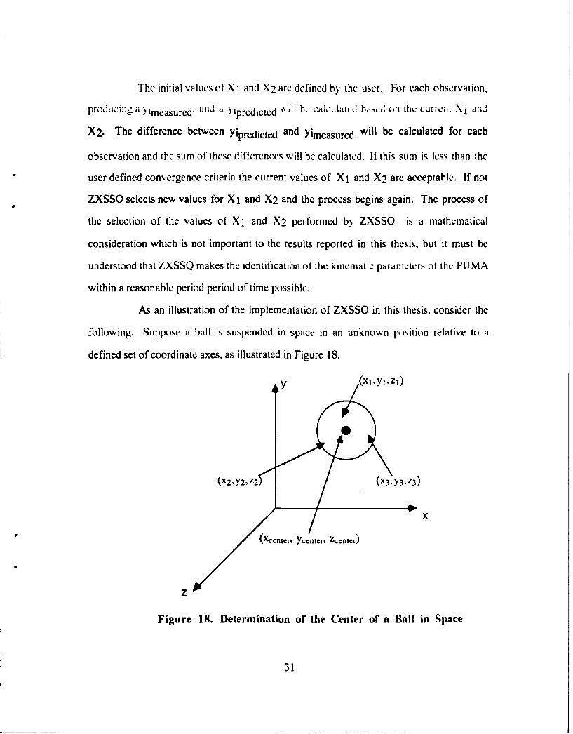
As an illustration of the implementation of ZXSSQ in this thesis, consider the

following. Suppose a ball is suspended in space in an unknown position relative to a

defined set of coordinate axes, as illustrated in Figure 18.

y (xi-y,.z 1 )

(x2-YY2Z2 , (x/ , yz-3)

* (Xcenter, Ycenter, Zcenter)

z

Figure 18. Determination of the Center of a Ball in Space

31

It is possible to use a touch probe to measure (xiYiZi), the coordinates of an A

position on the surface of the ball relative to the fixed coordinate frame. However. the exact

position of the center of the ball is required in order to assist in the determination of the

pose of the tool. ZXSSQ accepts the coordinates of at least three surface positions on the

ball and calculates the coordinates of the center of the ball. The procedure is as follows.

The end effector used in the experimental phase of the initial calibration has a

pattern of precision tooling balls which have a known radius, Rtb. The touch probe also

has a known radius, Rtp. That means that the center of the ball will be (Rtb + Rtp) from

each measured position of the touch probe. If only one touch probe measurement is made

the actual position of the center of the ball could be at any position on a sphere of (Rtb +

Rtp) radius surrounding the single measurement. As more measurements are taken the

position of the center of the ball can be determined more accurately. It has been determined

that a minimum of three touch probe measurements are required to accurately determine the

coordinates of the center of the ball. Each measurement produces an error function:

F, = (Rib + Rip)-\ (xC -x)2 + (C-Y- + (4 =z)2

F2 = (Rtb + Rip) - + (Y,-y2 + 1

F3 = (Rib + Rip)- (xc "X3j +(Yc "Y3) 2 + (: "z3)'z (28)

ZXSSQ will systematically vary (xc, yc,zc) until each Fi is minimized. If there

is no noise in the system, each Fi will be reduced to zero. If noise is present the best fit

(Xc.Yc,zc) will be calculated. Once the functions are minimized, the coordinates of the

center of the ball are known.

32

3. Application to the Calibration Process

The kinematic parameter identification of the PUMA 560 will be performed as a

multi-dimensional minimization process performed by ZXSSQ. The process will proceed

in the following manner.

1. Begin with the nominal set of kinematic parameters. This set will most

likely be the manufacturer's predicted parameters based on the design and construction of a

generic manipulator.

2. Select a set of six joint angles, 0 1 through 06. for the manipulator.

3. Perform a forward kinematic solution tor the PUMA. using the nominal set

of kinematic parameters. This will calculate the predicted pose of the end elector of the

manipulator.

4. Measure the actual pose of the end effector of the manipulator. In most

cases measured pose will be different from the predicted pose.

5. Modify the kinematic parameters such that the predicted pose, determined

by the forward kinematic solution using the modified kinematic parameters. matches the

measured pose [Ref. 8].

This process will be applied to several sets of joint angles. The number of

physical measurements, meaning the number of sets of joint angles required, must satisfy:

KP NxDf (29)

where: Kp = number of kinematic parameters to be identified

N = number of measurements (poses) taken

Df = number of degrees of freedom present in each measurement

Two calibration processes will be reported in this thesis. Each of the calibration

procedures will have a simulation phase and an experimental phase. The details of each

33

kinematic identification process will be described in each section of the appropriate

calibration procedure. Refer to the preceeding paragraph for a general explanation of the

kinematic parameter identification procedure.

34

III. FUI. POSF CALIBRATION

A. THEORY

1. Introduction

As stated earlier, the nominal coordinate transformations from the base frame to

frame 5 will not change, regardless of the type of calibration process used or the type of

measurement system used in the calibration. The transformation from the world coordinate

frame to the base frame is an Eulcr transform, as "ll as the transform from frame 5 to

frame 6, the tool frame.

The transformation from the world coordinate frame to frame I of the

manipulator needs to be carefully considered, since there arc potential parameter

dependencies if certain transforms are chosen. Consider Figure 19 which shows the world

coordinate frame xw,Yw,zw, frame xo,yozo, frame xb.Yb.zb, and frame xl,yl,zl.

Frame xo.Yo,zo is defined by a DH transform from the world frame to the first

joint axis of the manipulator, frame xb,Ybzb is the PUMA manufacturer's base frame and

frame x 1.Y 1.zl is the second DH frame of the manipulator. What are the minimum number

of parameters that are required to move from the world frame to frame x .y 1. z I ? There are

two transformation paths which will accomplish this transform [Ref. 9].

Path 1: A DH transform from the world coordinate frame to frame xo.yO.zo

involving four parameters followed by another DH from frame xo,yo,zo to frame xb,yb,zb

which will involve only two parameters0 and d in the transform:

T b = rot(zo,4')trans(z0,d') (30)

35

°° i/--.- p.,-

Figure 19. Base Transformations

Another DH transform from xb,yb,zb to xl,Yl,zl which involves four

parameters. Note that A01 and 4' both rotate about zo. That means that a rotation

A01 about the zo-axis is indiscernible. Any rotation about the z0-axis can be accomplished

using an infinite number of combinations of values of A01 and ', which means that

A01 and ' can not be identified independently. This leads to a conclusion that eight

independent kinematic parameters are required to move the coordinate frame from the world

frame to the first frame of the PUMA using this path.

Path 2: A transform can be defined directly from the world coordinate frame

xw,yw,Zw, to the base frame xb,Yb.zb. This is a frame to frame transform so an Euler

transform is required:

36

Ab = rot(z,4pb)rot(y,0t,)rot(xq,)trans(pxt,. P ," P) (31)

The DH transform from xb,Yb,zb to xl,Yl,zl which will follow would

normally involve four parameters, but there is another dependenc, involving A61 and

Ad,. A01 can be resolved into O.bl, and Ad, can be resolved into (PxbPytb.Pzb). This

reduces the number of parameters required for th. transform from the base frame to frame I

from four to two. Coupled with the six parameters required to transform from the world

frame to the base frame it is seen again that eight parameters are required to transform from

the world framc to tramc 1, but a different set of parameters than found in path 1. In this

simulation the second path is chosen.

The tool transform is an Euler transform, requiring the specification of six

parameters:

, = rot(z. o)rot(y.0 6)rot(x4q)6)trans(px 6,, p(,. P6) (32)

2. Full Model of the PUMA, Vorld Coordinate Frame, and

Coordinate Measuring Machine

Figure 20 shows the full pose calibration apparatus. The operation of the

coordinate measuring machine will be explained in the experimental section of this chapter.

37

Figure 20. Full Pose Calibration Apparatus: PUMA, World Coordinate

Frame and Coordinate Measuring Machine

Table 2 represents the kinematic parameters of the full pose model IRef. 10]. In

the full pose model all thirty parameters not previously defined to be zero, indicated in

boldface type, are able to be determined. Note the transform from the world coordinate

frame to the base frame of the PUMA.

38

TABLE 2. NOMINAL KINEMATIC PARAMETERS FOR THE FULL

POSE CALIBRATION

61, qIb Pxb Pyb Pzb

degrees degrees degrees mm mm mm

180.0 0.0 90.0 -394.0 -383.0 474.0

link AOi di ai a i Pi

number degrees mm mm degrees degrees

1 0 0 0.0 -90.0 02 0.0 0 431.85 0.0 0.0

3 0.0 149.09 -20.33 90.0 04 0.0 433.00 0.0 -90.0 0

5 0.0 0.0 0.0 90.0 0

66 0_ _6 Px6 Py6 Pz6

degrees degrees degrees mm mm mm

90.0 0.0 0.0 0.0 0.0 134.0

B. SIMULATION

I. The Suite of Programs Used and the Strategy Involved

In performing a simulation study of a proposed experimental calibration

procedure the objectives are to:

1. Confirm that the numerical algorithm proposed for the identification

converges to the correct values.

2. Predict the number of experimental poses required to identify the kinematic

parameters to a defined degree of accuracy.

3. Estimate the resulting accuracy of tht manipulator if the new kinematic

model was embedded in the control software of the manipulator [Ref. 11 .

39

Several computer programs were written to perform the simulation. These

programs. and their relationships to each other are shown in Figure 2 I.

PUMA-VAR.DAT

POSE -0

PUA-POS.DATE1 M 0

ID6 -

RESULT.DAT

vERIFY 1 POSVER.DAT

Figure 21. Flowchart for Full Pose Simulation

The complete simulation may be regarded as a tool to plan the experiment in

which the independent variables arc the number of observations and the range of joint

angles allowed by the common work volume of the PUMA and the coordinate measuring

machine, while the dependent variables are the accuracy of the parameter identification and

40

the resulting manipulator accuracy [Ref. 12]. A detailed explanation of each program

follows.

a. The program JOINT

Progra. i JOINT does not require an input data file.

Program JOINT generates sets of six joint angles which comprise a

simulated pose of the PUMA. The program can be modified such that the simulated

working volume of the PUMA is restricted from the maximum possible to either one-half

of one-quarter of the maximum volume.

The joint angles are selected using a random number generator. For

instance, if the working volume of the PUMA has been selected as the maximum possible,

the program takes the difference between the extreme joint angles possible, +180(-

180)=360, then multiplies this value by a number between 0 and 1. which has been

generated randomly. thus generating one joint angle. Since six independent joint angles are

required, six different random numbers and six different joint angles are generated for each

pose, or observation.

The output of program JOINT is a data file, PUMA-VAR.DAT PUMA-

VAR.DAT will have n sets of six joint angles, which comprise n simulated poses of the

PUMA. In the verification phase program JOINT is run again, with the output data file

being renamed POSEVER.DAT for use in program VERIFY.

b. The program POSE

Program POSE requires two input data files, PUMA-VAR.DAT, the

output data file from program JOINT, and INPUT.DAT, the nominal kinematic parameters

of the PUMA, listed in Table 1. POSE also inputs values "dangle" and "dlenth." The

value assigned to "dangle" is added to all of the angular parameters except for the ones

which are defined to be zero. The value assigned to "dlenth" is added to all of the length

41

parameters. Adding these values creates a manipulator which is significantly different from

the manipulator reflected in the nominal kinematic parameter table. and is equivalent to

supplying the kinematic identification program with pseudo-experimental data. Creating

this different manipulator tests the integrity of the kinematic parameter identification

program. Since the initial guess of the parameters will be the nominal parameters the

identification program must rigorously solve for the actual kinematic parameters, which

will be the nominal parameters plus "dangle" and "dlenth" as appropriate.

Program POSE generates a T6 matrix, representing the simulated position

and orientation of the tool frame of the PUMA. for each set of joint angles which were

generated by program JOINT.

When the joint angles are read from PUMA-VAR.DAT they are added to

the parameters read from the nominal kinematic table which apply to the individual joint.

For example, in POSE the variable THI equals the sum of DT1 and THETAL. DT1 is

input from the nominal kinematic table and THETAI has been generated by JOINT. The

nominal kinematic parameters are added to the simulated actual joint angles as any non-zero

THETA value at any joint represents a movement from the zero position of that joint.

Once the joint angles are calculated and the nominal kinematic parameters

are adjusted, a forward kinematic solution is calculated. This will produce one T6 matrix

for each set of joint angles. In order to accurately model an actual measurement in the

laboratory noise is added to the position vector of the T6 matrix and the six joint angles of

each simulated pose. The position noise arises from the uncertainty of the precision with

which the coordinate measuring machine and associated software is capable of identifying

the position of the center of a tooling ball. The position noise is generated by multiplying a

random number which is generated in the same manner as in JOINT by a number read from

INPUT.DAT "magnx." The joint angle noise, called the encoder error, is generated by

42

multiplying a random number by another value which is read from INPUTDAT. "magn I."

The position noise is 100 tims:- the: niagnit~u i of the cncoder noise.

The output of POSE will be the six joint angles for each simulated pose

and the corresponding T6 matrix for each set of joint angles. This data is stored in the

output file PUMA-POS.DAT.

c. The program ID6

Program I1D6 requires two input files, INPUT.DAT and PUMA-

POS.DAT. The nominal kinematic parameters are read from INPUT.DAT in order to

provide the kinematic parameter identification with a beginning point. The T6 matrices

contained in PUMA-POS.DAT which were generated by program POSE contain the

simulated poses with which the actual kinematic parameters will be identified in this

program.

ZXSSQ will perform the kinematic parameter identification. The function

to be minimized by ZXSSQ is actually an array of six functions. Each pose will have six

functions to be minimized, so if there are ten poses, or observations, ZXSSQ will have

sixty functions to minimize using thirty variables.

A subroutine within ZXSSQ, PUMAARM. calculates the T6 matrix

corresponding to the current kinematic parameters for each set of six joint angles input from

PUMA-POS.DAT The simulated measured T6 matrix read from PUMA-POS.DAT for

each set of joint angles is known. Since the original nominal kinematic parameters were

altered before the simulated measured T6 matrix was calculated, the simulated measured T6

matrix will be different from the T6 matrix calculated using the generated joint angles and

the nominal kinematic parameters. Also, the added measurement noise is present,

providing more of a difference in the two matrices. For each observation the array of six F

functions is calculated. After performing the matrix subtraction:

43

AT Tm,surcd' -Tcal,:, ,,',:d- (33)

the six F functions are determined for each observation:

F 1 = AT(1.4)

F 2 = AT(2.4)

F3 = AT(3,4)

F4 (AT(3.2) - AT(2.3))F4= ( _)2 x scaling factor

Fs-(AT(l,3) - AT(3,1))...... ..... .. .=× scaling factor

2

F6 = (AT(2,1) -AT(1,2)) x scaling factor2) (34)

The scaling factor which multiplies the functions in equation (34) is used

to remove the emphasis from the position error. The position error in a pose will be much

larger than the orientation error between two T6 matrices. For this reason the emphasis in

the optimization program will be on eliminating the position error. while largely ignoring

the orientation error. This is unacceptable, since the orientation error is equally important

as the position error. The scaling factor places the orientation error at the same level of

magnitude as the position error.

The F functions in equation (34) represent the error matrix [Ref. 13]:

0 -bz by d,

bz 0 -bx dy

-6) bX 0 d,

0 0 0 0 (35)

It must be noted that equation (35) can only be used when the two

matrices being subtracted are almost equal. In an actual experimental process the measured

poses usually significantly differ from the predicted pose. This difference causes the A

44

matrix, equation 35, to have relatively large elements. ZXSSO is often unable to converge

under these conditions. The different version of ID6 will be introduced in the Experimental

section of this chapter.

After all the observations have been calculated for each pose, ZXSSQ

compares each F value with a user defined convergence criteria. Convergence is defined

when the kinematic parameters selected from one iteration to the next agree to four

significant digits. If every F for each pose is less than this convergence criteria, then the

current kinematic parameters are saved as the correct parameters. If not. ZXSSQ changes

the thirty kinematic parameters and performs the process again until the convergence criteria

is satisfied.

The output of ID6 is RESULTDAT. The identified kinematic parameters

will be stored in the same format as INPUT.DAT. In the simulation the identified

kinematic parameters will be the parameters of INPUT.DAT plus dangle for orientation

parameters and dlenth for length parameters plus some small error value created by the

addition of the simulated measurement noise.

d. The program VERIFY

Program VERIFY requires three input programs. The first.

POSEVER.DAT, is the output from program JOINT, and includes sets of six joint angles.

The other two are kinematic parameters, INPUT.DAT and RESULT.DAT. INPUT.DAT,

as explained earlier, contains the nominal kinematic parameters, and RESULT.DAT

contains the kinematic parameters identified in program ID6.

VERIFY measures the position and orientation difference between poses

calculated using the nominal kinematic parameters and the nominal kinematic parameters.

For each set of joint angles, VERIFY calculates a forward kinematic solution using both the

nominal and identified kinematic parameters and takes the difference between the

45

corresponding T6 matrices. The position error and orientation error for all of the sets of

joint angles are added and these values are divided by the total number of sets of joint

angles. This will produce the total position error and total orientation error for a given

number of observations.

C. EXPERIMENTATION

1. The Tooling Ball End Effector

The tooling ball end effector is illustrated in Figure 22. Its' purpose is to

provide a means for determining the position and orientation of frame 6 of the PUMA. The

five balls attached to the effector are precision tooled to a radius of 6.35 mm. This known

radius, along with the known radius of the touch probe of the coordinate measuring

machine provides the essential information required for identification of the center of each

tooling ball by the routine BALL described earlier in the thesis. Also, each of the four

tooling balls contained in the plane normal to the axis of the effector are nominally 90

degrees apart, creating orthogonality between any two in series around the circumference of

the tool. The fifth tooling ball's center lies on an axis which passes the two lines which

attach balls on opposite sides of the tool, creating another orthogonality between the fifth

ball and each of the other four. The orientation of frame six is fixed on the tool and is

required information for the determination of the position and orientation of the tool frame

by program CMMPOSE.

46

Sz6

x 6 ," 6xY6

Figure 22. Tooling Ball End Effector

2. The Coordinate Measuring Machine and World Coordinate Frame

a. Construction

The coordinate measuring machine (CMM) used for data acquisition in

this thesis is illustrated in Figure 23.

47

Y Y -axris recep tacle

Z- axis receptacle

X-axis receptacle

Figure 23. Coordinate Measuring Machine

The x-axis lies on the base of the CMM. Rotating the x wheel will move

the x-axis receptacle to the left or right, changing the x-value displayed. The y-axis is

contained within a post which is attached to the slide that changes the x position. Rotating

the y wheel moves the y-axis receptacle up or down, changing the y-value displayed. The

z-axis is contained is the y-axis receptacle assembly. Rotating the z wheel moves the z

receptacle in or out, changing the z value displayed. Consider the point (1,1,1) relative to a

known world reference frame. Rotating the x wheel will produce a change in position

(Ax,1,1). Rotating the y wheel will produce a change in position (l,Ay,l). Rotating the z

48

wheel will produce a change in position (I,l,Az). It is clear that any point in the working

volume of the CMM may be reachcd by the touch probe.

A siLnific:nP. d\,intao' c t ( thi, C NII i, j1 , ahili!, to Zero :1 an\ pO.itio:.

Each axis may be zeroed independently or concurrently. This is important in identifying

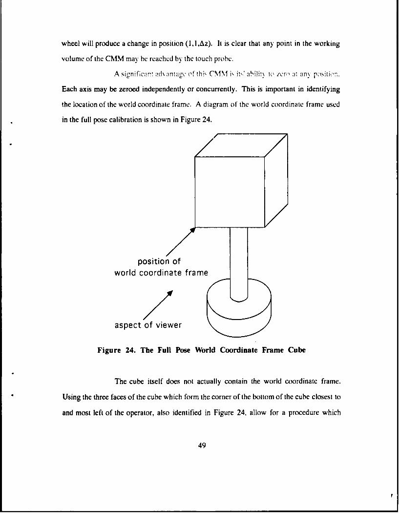
the location of the world coordinate frame. A diagram of the world coordinate frame used

in the full pose calibration is shown in Figure 24.

position ofworld coordinate frame

aspect of viewer

Figure 24. The Full Pose World Coordinate Frame Cube

The cube itself does not actually contain the world coordinate frame.

Using the three faces of the cube which form the corner of the bottom of the cube closest to

and most left of the operator, also identified in Figure 24, allow for a procedure which

49

identifies point (0,0,0) of the world coordinate frame. Once this point is identified, the

axes o1 the world coordinate trarmn match mc axes ot the CMM. The procedure ltr

identifying the world coordinate frame is as follows. Note that the order of the

identification process of the world coordinate frame is arbitrary.

1. The touch probe is positioned in area near the bottom, left, forward

face of the cube.

2. Activate the 'x-zero' mode of the CMM. Move, using all three axes

if necessary, the touch probe such that its' position is as close to the forward corner of the

bottom of the left face as possible. Slowly move the probe to the right, using the x-axis

wheel only, until contact is made with the forward face of the cube. When contact is made

the display unit (DU) will beep and the x position will indicate zero.

3. Activate the 'y-zero' mode of the CMM. Move. using all three axes

if necessary, the touch probe such that its' position is as close to the forward, left corner of

the bottom face of the cube as possible. Slowly move the probe upwards, using the y-axis

wheel only, until contact is made with the bottom of the cube. When contact is made the

DU will beep and the y position will indicate zero.

4. Activate the 'z-zero' mode of the CMM. Move, using all three axes

if necessary, the touch probe such that its' position is as close to the bottom. left corner of

the forward face of the cube as possible. Slowly move the probe towards the cube. using

the z-axis wheel only. until contact is made with the forward face of the cube. When

contact is made the DU will beep and the y position will indicate zero.

Once this procedure is completed a point in space located a distance equal

to the diameter of the touch probe along each axis, (diajYdia,J,jZdia,j), will be identified as

the location of the world coordinate frame. This process is easily repeatable and has a high

50

degree of accuracy, so for different sets of experimental measurements the position of the

world coordinate frame should not vary to a significant degree.

b. Data Acquisition Using the Coordinate Measuring Machine

Data acquisition using the coordinate measuring machine consists of a

repetitive measurement of the position of three different tooling balls on the end effector

illustrated in Figure 22. The PUMA is operated in joint mode. which allows each of the six

joints to be rotated independently. The end effector, which is attached to the tooling ball

assembly, is moved to a variety of positions. When the operator is satisfied with the

position of the tool, the measurement process begins.

Execution of the pose measurement program, CMMPOSE, begins by

inquiring which tooling ball on the tool is being measured. This information is required in

order to determine the orientation of frame 6. The touch probe of the CMM is moved

slowly towards the selected tooling ball. As the probe touches the surface of the ball the

display unit of the CNM beeps. The position displayed by the unit is the position of the

probe at the first instant that the probe touches the surface of the ball, and is displayed in

millimeters to two significant digits. If the probe slightly slides after initial contact the

displayed position will not change, remaining until one of the three axes of the CMM is

moved. CMMPOSE asks for three touch probe measurement sets per ball and determines

the center of each tooling ball using the procedure described in section II.B.2. Once the

center of each ball is calculated a residual error reflecting the uncertainty of the accuracy of

the predicted position of the center of the ball is displayed. An option of storing or purging

the data is given at this point. Based on the judgement of the operator, the data is sent for

further manipulation by CMMPOSE, or the data is purged and another set of ball

measurements is taken. An acceptable residual error has a value near 0.000001 mm. Once

the center of three of any of the five tooling balls, P1, P2, and P3, is determined, the

51

program synthesizes the position of the center of a fourth ball, P4. by calculating the vector

cross product [Ref. 141:

P4 = (P3 -P) X (P2 -PI) (36)

The relationship between the coordinates of the center of each ball

expressed in terms of the tool frame and the world coordinate frame is

P =.A IPj (37)

where Pi* is the 4x1 column vector of the coordinates of the ith ball

expressed with respect to the world frame, Pi is the 4xI column vector ol the coordinates

of the ith ball with respect to the tool frame, and A is the 4x4 homogeneous transformation

matrix from the world frame to the tool frame.

If Pi is known by precalibrating the tool. and Pi* is measured then A may

be calculated and used as the measured pose in the calibration process. The difficulty arises

in inverting equation (37) to obtain A. The following information is known:

~Pi = A"P 1 'P-= A -P2 '

:P;="A P3LP4J = [A} LP4. (38)

Algebraic manipulation produces:PP2 P3 P4 = 'A' Pi P2 'P3 P4 (39)

reducing:

LP=A P (40)

52

Since P*, A, and P are all 4x4 matrices, equation (40) can be inverted.

producing matrix A. the pose of thc tool:

AI =P' P'l (41)

Two operators can expect to measure one pose in ten minutes. One

operator will be utilized to move the PUMA and operate the CMM and the other operator

will input data as instructed by program CMMPOSE.

c. Identification of Actual Kinematic Parameterx

A modified version of program ID6 is used for the identification of the

actual kinematic parameters of the PUMA. The modification is in the functions which are

minimized by the IMSL routine ZXSSQ. As mentioned earlier, the delta matrix of equation

(35) is suitable for use only when the predicted pose and the measured pose are quite

close. Experimentation will usually produce matrices which arc dissimilar. For this

reason, each element of the matrix resulting from the difference between the predicted and

measured pose is minimized:

F1 F 4 F 7 Flo - a,1 a12 a13 a14 - all a12 a13 a14F2 F5 F8 F11 a21 a,, a23 a24 a21 a22 a23 a2 4F 3 F6 F 9 F 1 2 a3 1 a3 2 a3 3 a 3 4 a31 a3 2 a33 a3 4

0 0 0 1 0 0 0 1 -predicted 0 0 0 1 measured

(42)

This produces twelve functions which are to be minimized. This method

provides a more rigorous method for the identification of the kinematic parameters. Table 3

shows the kinematic parameters identified using the full pose calibration procedure [Ref.

155.

53

TABLE 3. FULL POSE IDENTIFIED PARAMETERS

Parameter Nominal Value Identified Value

9t 180.0 179.9579

61_ 0.0 1.5120

Tb 90.0 89.0219

Pxb -394.0 -393.9838

Pyb -383.0 -405.0608

Pzb 474.0 466.8381

a, 0.0 -0.0 923at1 -90.0 -89.9977

60, 0.0 -0.4888

a: 431.9 432.1216

Ct_ 0.0 .0.0303P_2 0.0 -0.01515

603 0.0 -1.2069

d, 149.1 149.1455

al -20.3 -19.2270

a, 90.0 90.0512

b 4 0.0 -0.9144

d4 433.0 432.8899

a4 0.0 0.0040

a4 -90.0 -89.9909

b0.s 0.0 2.2364

d s 0.0 -0.6629

as 0.0 -0.0258

a-s 90.0 89.9345

_ _ 90.0 91.2400

06 0.0 -0.0979

(P6 0.0 -0.0575

Px6 0.0 0.1863

P,6 1 0.0 -0.2329

pz6 134.0 133.1557

54

IV. PARTI MI POSE CALIBRATION

A. THEORY

1. Introduction

As stated earlier, the nominal coordinate transformations from the base frame of

the manipulator to frame 5 will not change. These transformations are inherent to the

manipulator and are independent of the pose measurement scheme being employed. The

transformations from the world coordinate frame to the base frame and from frame 5 to

frame 6 are the same transformations as employed in the full pose calibration.

The world coordinate frame is not in the same position, and is not defined in the

same manner, as it was in the full pose calibration. The partial pose calibration

measurement system uses a linear slide to which the tool frame of the manipulator is

attached. The only variable which is measured is the position of the slide relative to a zero

position defined at the beginning of each pose measurement session. The world frame is

defined as the T6 matrix of the tool when the slide's position on the slide equals zero. The

slide acts as a prismatic joint and hence is defined only in direction. The location of the

axis is undefined. The three translational components of the transform from frame five to

frame six, V15, are arbitrary and may be set equal to zero. This defines that the origins or

frame five and six are coincident, as shown in Figure 25. This will reduce the full thirty

parameter model to twenty-seven parameters.

The world coordinate frame's orientation is not known, either. The direction of

one axis is able to be defined. In this experiment the axis of the linear slide has been

defined as the x axis. The y and z axes of the world coordinate frame are orthogonal to the

55

x-axis, but their orientation relative to the x-axis is undefinable, arbitrary, and therefore set

equal to Lero. This lurther reduces the model to twcnt)-six parameters.

0 9o Axis of Lneor SI;Je

Figure 25. Linear Slide Transformations

The partial pose calibration model dictates that the tool frame pose is invariant.

Each pose will have the following orientation:1 00 X

0 0-1 00 1 0 00 0 0 1 (43)

This T6 matrix defines the x-axis of the tool frame to be in the same direction as

the x-axis of the world coordinate frame, the y-axis of the tool frame to be in the same

direction as the z-axis of the world coordinate frame, and the z-axis of the tool frame to be

in the same direction as the negative y-axis of the world coordinate frame. Also, the

56

position of the origin of frame six is at position (X,0,0), where X is the position of the

linear slide. Note that it is still not possible to uniouelv define the orientation of the world

coordinate frame with respect to any frame on the PUMA. It is only known that the

orientation of the world coordinate frame is consistently defined with respect to the

orientation of the tool frame.

2. Full Model of the Puma and the Linear Slide

Figure 26 shows the partial pose calibration apparatus. The operation of the

coordinate measuring machine as a linear slide will be explained in the experimental section

of this chapter.

Figure 26. Partial Pose Calibration Apparatus: PUMA and Linear Slide

57

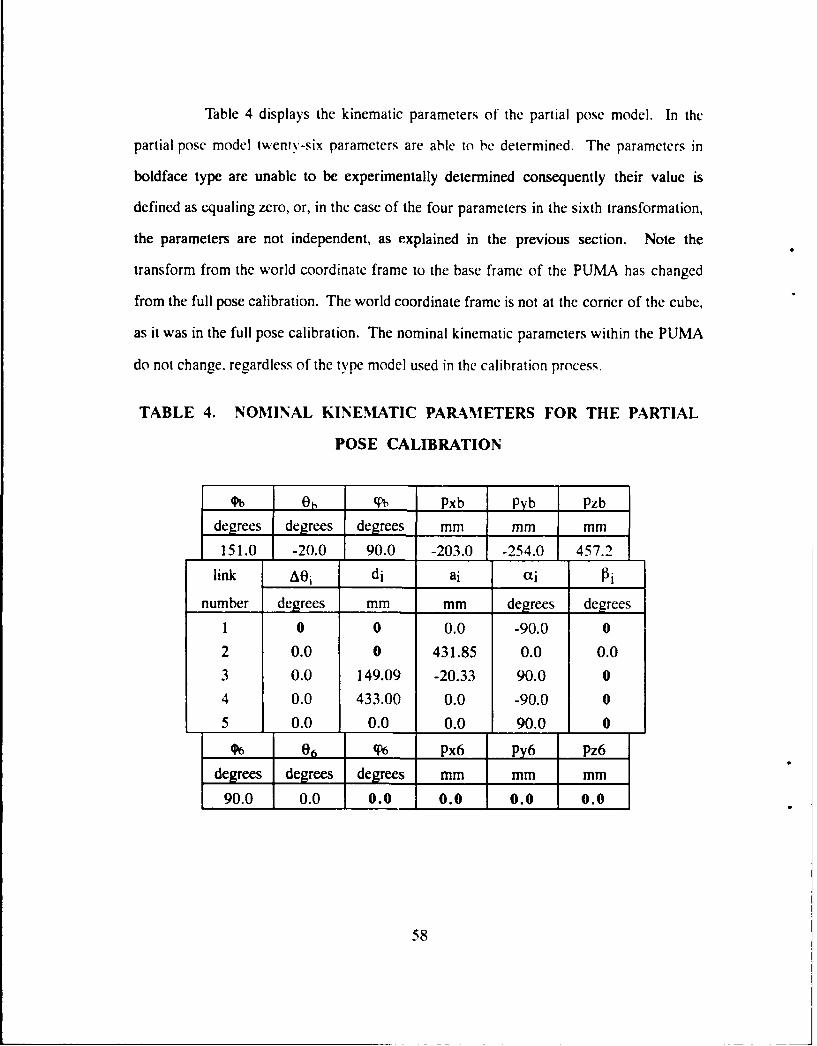
Table 4 displays the kinematic parameters of the partial pose model. In the

partial pose model twenty,-six parameters are able to be determined. The parameters in

boldface type are unable to be experimentally determined consequently their value is

defined as equaling zero, or, in the case of the four parameters in the sixth transformation,

the parameters are not independent, as explained in the previous section. Note the

transform from the world coordinate frame to the base frame of the PUMA has changed

from the full pose calibration. The world coordinate frame is not at the corner of the cube,

as it was in the full pose calibration. The nominal kinematic parameters within the PUMA

do not change. regardless of the type model used in the calibration process.

TABLE 4. NOMINAL KINEMATIC PARAMETERS FOR THE PARTIAL

POSE CALIBRATION

% 0 Tb Pxb Pyb Pzb

degrees degrees degrees mm mm mm

151.0 -20.0 90.0 -203.0 -254.0 457.2link Ae, di ai ai Pi

number degrees mm mm degrees degrees

1 0 0 0.0 -90.0 0

2 0.0 0 431.85 0.0 0.03 0.0 149.09 -20.33 90.0 04 0.0 433.00 0.0 -90.0 0

5 0.0 0.0 0.0 90.0 0

96 06 TP6 Px6 Py6 Pz6

degrees degrees degrees mm mm mm

90.0 0.0 0.0 0.0 0.0 0.0

58

B. SIMULATION

1. The Suite of Programs Lsed and the Strateg) Intoied

As stated earlier, the simulation study is performed to:

1. Confirm that the numerical algorithm proposed for the identification

converges to the correct values.

2. Predict the number of experimental poses required to identify the kinematic

parameters to a defined degree of accuracy.

3. Estimate the resulting accuracy of the manipulator if the new kinematic

model was embedded in the control software of the manipulator.

In the partial pose calibration, the forementioned "correct" values arc the

kinematic parameters identified using the full pose method. The computer programs

written, and their relationships, are illustrated in Figure 27.

LUNSC

ID6_linsc

RESULT.DAT

Figure 27. Flowchart for Partial Pose Simulation

59

The complete simulation may be regarded as a tool to plan the experiment in

which the independent variables are the number of observations and the range of joint

angles allowed by the common work volume of the PUMA and the linear slide, while the

dependent variables are the accuracy of the parameter identification and the resulting

manipulator accuracy. A detailed explanation of each program follows.

a. The program LINSC

Program LINSC requires the input file INPUTDAT, the nominal

kinematic data for the PUMA, which are listed in Table 1. LINSC also inputs values

"dangle" and "dlenth," as did program POSE in the simulation phase of the full pose

calibration. It will be instructive to reexamine the function of these two parameters. The

value assigned to "dangle" is added to all of the angular parameters except for the ones

which are defined to be zero. The value assigned to "dlenth" is added to all of the length

parameters. Adding these values creates a manipulator which is significantly different from

the manipulator reflected in the nominal kinematic parameter table. and is equivalent to

supplying the kinematic identification program with pseudo-experimental data. Creating

this different manipulator tests the integrity of the kinematic parameter identification

program. Since the initial guess of the parameters will be the nominal parameters the

identification program must rigorously solve for the actual kinematic parameters, which

will be the nominal parameters plus "dangle" and "dlenth" as appropriate.

Program LL\NSC generates six joint angles which will produce a T6

matrix with an orientation that is predefined and fixed and a position on the slide which has

been randomly generated. This is done by performing an inverse kinematic solution, since

the T6 matrix is known. The set of joint angles, when used with the nominal kinematic

parameters of the PUMA, which will produce the required T6 matrix is the required data.

The IMSL routine ZXSSQ is again used to make this determination.

60

ZXSSQ uses an initial guess of all six joint angles equaling zero. A

forward kincma"! *. , snlwi- is calcuhMld haicd on thCY,' jOirt anC(, ard the nominal

kinematic parameters plus dangle and dlenth. The difference between each element of the

calculated T6 matrix and the required T6 matrix is calculated. These elements represent the

functions to be minimized:

F 1 F 4 F 7 Flo all a12 a1 3 a1 4 all a 12 a1 3 a14

F 2 F 5 F 8 F11 a21 a2 2 a2 3 a2 4 a21 a2 2 a2 3 a24

F 3 F 6 F 9 F 1 2 a31 a3 2 a33 a34 a31 a32 a33 a34

0 0 0 1 0 0 0 1 -:predicted 0 0 0 1 -measured

(44)

ZXSSQ modifies the joint angle set until a convergence criteria is

satisfied. At convergence the required T6 matrix and the six joint angles are returned to the

main program.

It has been stated that in order to accurately model an actual measurement

in the laboratory noise must be added to the simulated T6 matrix and the six joint angles of

each pose. The position noise and encoder noise is generated in the same manner as in

program POSE in the full pose simulation. The position noise in the partial pose simulation

arises from the uncertainty in the measurement of the position of the slide. The orientation

error arises from inconsistencies in the bar supporting the slide. The bar almost certainly

will have elements of twist and bend in it. These elements will cause differences in

orientation as the slide moves along its' length.

After the noise is added to the T6 matrix and the joint angles, the data is

stored in the output file PUMA-POS.DAT.

b. The program ID6_,INSC

Program ID6_linsc requires two input files, INPUT.DAT and PUMA-

POS.DAT. The nominal kinematic parameters are read from INPUT.DAT in order to

61

provide the kinematic parameter identification with a beginning point. The T6 matrices and

associated joint angles contained in PUMA-PUS.DAI which were generated b) program

LINSC contain the simulated poses with which the actual kinematic parameters will be

identified in this program.

ZXSSQ will perform the kinematic parameter identification. Each element

of the matrix resulting from the difference between the predicted and measured pose is

minimized, as was done during the actual kinematic parameter identification of the full pose

calibration method. See equation (43) for the equation of the functions to be minimized.

This produces twelve functions which arc to be minimized. Subroutine

PUMAARM calculates the T6 matrix corresponding to the current kinematic parameters

for each set of six joint angles input from PUMA-POS.DAT The simulated measured T6

matrix read from PUMA-POS.DAT for each set of joint angles is known. Since the

original nominal kinematic parameters were altered before the simulated measured T6

matrix was calculated, the simulated measured T6 matrix will be different from the T6

matrix calculated using the generated joint angles and the nominal kinematic parameters.

Also, the added measurement noise is present, providing more of a difference in the two

matrices.

After all the observations have been calculated for each pose. ZXSSO

compares each F value with a user defined convergence criteria. Convergence is defined

when the kinematic parameters selected from one iteration to the next agree to four

significant digits. If every F for each pose is less than this convergence criteria, then the

current kinematic parameters are saved as the correct parameters. If not, ZXSSQ changes

the twenty-six available kinematic parameters and repeats the process until the convergence

criteria is satisfied.

62

The output of ID6_linsc is RESULTDAT. The identified kinematic

paramcten wil! hc stored in the same format a- INPI T.DAT. In the simulation the

identified kinematic parameters will be the parameters of INPUTDAT plus dangle for

orientation parameters and dlenth for length parameters plus some small error value created

by the addition of the simulated measurement noise.

C. EXPERIMENTATION

1. The Coordinate Measuring Machine as a Linear Slide

a. Construction

The coordinate measuring machine's base, which supports the x-axis, is

mounted on an incline, as illustrated in Figure 28. The incline is placed on the table on

which the PUMA is mounted, in an orientation which is significantly different from the x-

axis of the PUMA. This position, concurrent with the inclined mounting. provides for the

maximum possible joint rotation of all six joints of the PUMA.

63

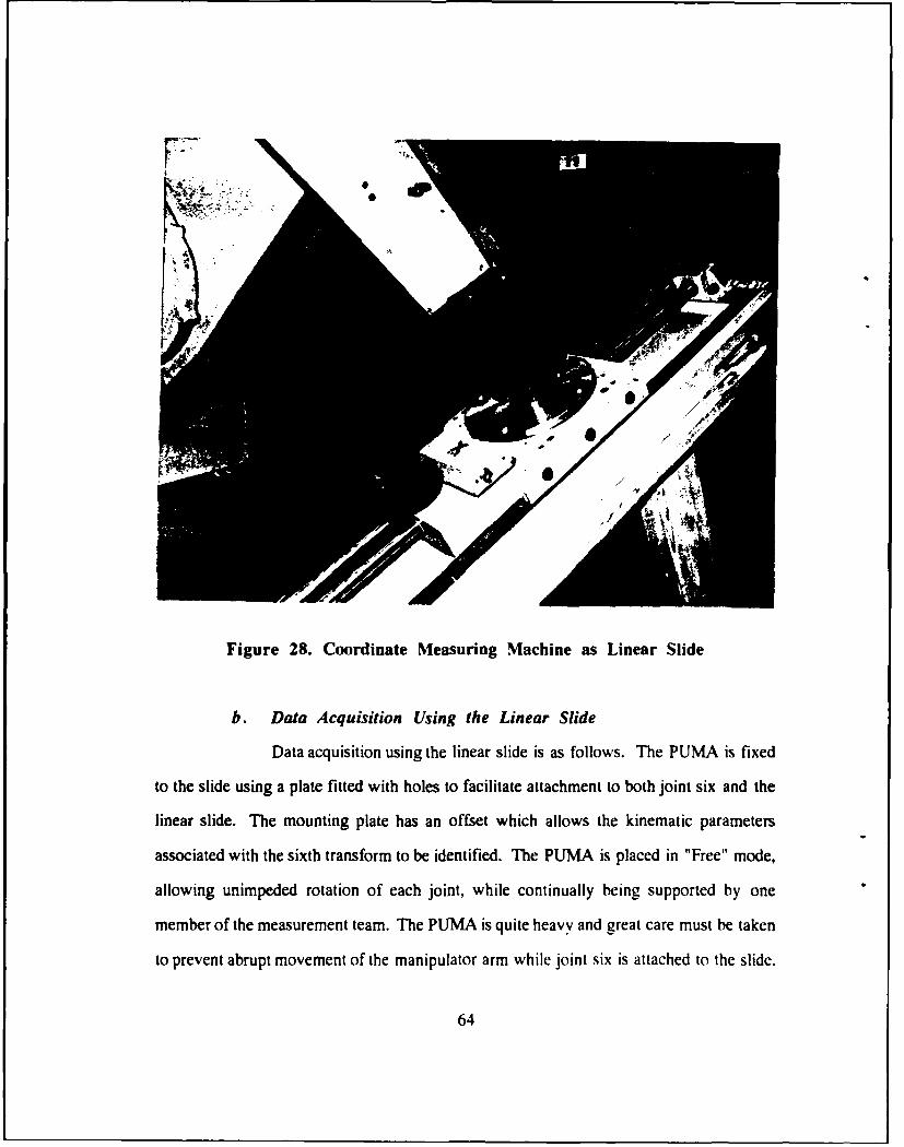
r7p

Figure 28. Coordinate Measuring Machine as Linear Slide

b. Data Acquisition Using the Linear Slide

Data acquisition using the linear slide is as follows. The PUMA is fixed

to the slide using a plate fitted with holes to facilitate attachment to both joint six and the

linear slide. The mounting plate has an offset which allows the kinematic parameters

associated with the sixth transform to be identified. The PUMA is placed in "Free" mode,

allowing unimpeded rotation of each joint, while continually being supported by one

member of the measurement team. The PUMA is quite heavy and great care must be taken

to prevent abrupt movement of the manipulator arm while joint six is attached to the slide.

64

The slide is moved to one end of the slide and the x-axis position indicator on the display

unit is zeroed. The slide should be positioned at the lower end of the slide when being

zeroed in order to have positive x-axis position indications on the display unit. The slide is

moved up the scale in incremental distances, and after each increment the six joint angle

positions of the PUMA and the x position of the slide is input using program ACDAT. The

position which has been input is stored with the orientation matrix, which will not change,

regardless of the position of the slide.

Two operators can expect to measure one pose in one minute. One

operator is utilized to move and support the PUMA while the other will input the position

of the slide and the joint angles of the PUMA, as directed by program ACDAT.

c. Identification of Actual Kinematic Parameters

The same version of program ID6_linsc which was used in the

identification of the kinematic parameters in the simulation phase of the partial pose

calibration is used in the identification of the actual kinematic parameters. Table 5 shows

the kinematic parameters identified using the full pose calibration procedure.

65

TABLE 5. PARTIAL POSE IDENTIFIED PARAMETERS

Parameter Nominal Value Identified Value

151.0 150.4016

0t -20.0 -18.1370

9b 90.0 90.1163

pxh -203.0 -167.1160

P vb -254.0 -382.9224

pzb 457.2 408.2330

al 0.0 0.3920

Ct . -90.0 -89.9778

60 2 0.0 -0.5600

a-) 431.85 431.9559

a. 0.0 -0.0648

p 2 0.0 0.0326

600.3 0.0 -1.0704

d3 149.1 149.4573

a. -20.3 -19.3452

_l 90.0 90.1312

60 4 0.0 -0.8549

d 4 433.0 433.0048

a4 0.0 0.6809

(14 -90.0 -89.5235

605 0.0 2.3123

ds 0.0 -0.3900

a5 0.0 -0.8460

as_ 90.0 89.5360

_ _ _ 90.0 78.6654

6 0.0 -0.1972

66

V. DISCUSSION OF RESULTS

A. GENERAL OBSERVATIONS

Both the full pose and partial pose calibration methods successfully provided

kinematic parameters which could be used in a control program to use the PUMA most

accurately. Each simulation predicted convergence to a unique set of kinematic parameters,

thirty for the full pose method and twenty-six for the partial pose method. Poses measured

in the laboratory provided the data which proved this prediction.

The results of the kinematic parameter identification using the full pose calibration

method indicates that the resulting accuracy of the manipulator is 0.3 mm. The

experimentally predicted accuracy was considerably larger than the predicted accuracy from

the simulation, which was approximately 0.15 mm. This is most likely attributed to a

higher magnitude of noise being present in the pose measurements than predicted in the

simulation. It may be concluded that using this type of calibration method will improve the

accuracy of the manipulator to about the same value of the manipulator repeatability [Ref.

16].

The results of the kinematic parameter identification using the partial pose calibration

method indicate that the resulting accuracy of the manipulator is 0.9 mm. It may be

concluded that using this type of calibration method will provide a manipulator which is

three times less accurate than a manipulator calibrated using the full pose method, but still

more accurate than an uncalibrated manipulator.

The method to determine accuracy of the partial pose calibration method is as follows.

A total of 42 poses were measured, 21 in lefty configuration, 21 in righty. The lefty and

righty configuration is a description of joint l's position. If, while the operator is facing

67

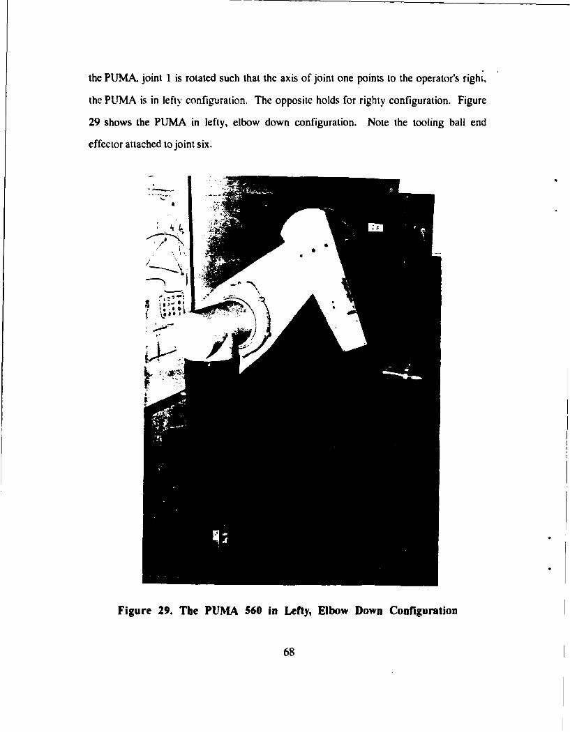
the PUMA, joint 1 is rotated such that the axis of joint one points to the operator's right,

the PUMA is in lefty configuration. The opposite holds for righty configuration. Figure

29 shows the PUMA in lefty, elbow down configuration. Note the tooling ball end

effector attached to joint six.

Figure 29. The PUMA 560 in Lefty, Elbow Down Configuration

68

While all 42 poses were used in the identification of the kinematic parameters shown

in Table 5, to determine the accuracy, the poses were divided. T-ic first ten poses

measured in the lefty and righty configuration were merged to form a set of twenty poses

which were used in program ID6_LINSC to determine a set of identified kinematic

parameters, an output file KINPARAM.DAT The last ten poses measured in the lefty and

righty configuration were merged into a data file, MEASURE.DAT, to act as the measured

poses. The program EFOR was executed, calculating the predicted poses based on the

actual joint angles of the PUMA, read from MEASURE.DAT, and the identified kinematic

parameters. read from KINPARAM.DAT. The result is two sets of "6 matrices, one the

actual measured T6 matrix, the other the predicted T6 matrix. Program COMP.FOR

calculates the RMS position difference and orientation difference between the two sets of

T6 matrices.

B. COMPARATIVE OBSERVATIONS

Table 6 shows the identified kinematic parameters for the PUMA using the full pose

calibration method and the partial pose calibration method. A comparison of the two

methods of calibration described in this thesis, along with an analysis of the identified

calibrated parameters, will follow.

69

TABLE 6. COMPARISON BETWEEN FULL AND PARTIAL POSE

IDENTIFIED KINEMATIC PARAMETERS

Parameter Nominal Value Identified Value Identified Value

___________ __________ FULL POSE PARTIAL POSE

al 0.0 -0.04923 0.3920

a, -90.0 -89.9977 -89.9778

602 0.0 -0.4888 -0.5600

a2 431.9 432.1216 431.9559

a' 0.0 -0.0303 -0.0648

02_______ 0.0 -0.015 15 0.03.26

60; 0.0 -1.2069 -1.0704

d_________ 149.1 149.1455 149.4573

a;________ -20.3 - 19. 227 0 -19.3452

___ _______ 90.0 90.0512 90.1312

604 0.0 -0.91 44 -0.8549

d4 433.0 432.8899 433.0048

a4 0.0 0.0040 0.6809

q 4 -90.0 -89.9909 -89.5235

605 0.0 2.2364 2.3123

__________ 0.0 -0.6629 -0.3900

a______5 __ 0.0 -0.0258 -0.8460

a___ -j____1 90.0 89.9345 1 89.5360 _

Most robot manipulator arms will be used in an industrial environment. While it is

important that the manipulator be properly calibrated, the amount of time the manipulator is

unavailable for operation due to the calibration process being performed is significant. The

experiments performed clearly have shown the full pose method takes considerably more

time to accomplish than the partial pose method. The full pose method takes approximately

70

ten minutes to make one pose measurement, while the partial pose measurement takes only

one minute to measure one pose. The amount of time required could be cut dramatically if

an intcrfd, ,: between the PUMA .on'..... con-,pi', c and the data acquisition computcr 'A r,

built. This interface would eliminate the need for manual entry of the six joint angles for

each pose. The relative difference in the amount of time required to measure one pose

would still be present.

The full pose calibration method provides for a more accurate calibration of the

manipulator. This fact arises from two considerations. First, more of the kinematic

parameters of the manipulator can be identified using the full pose method, thirty, than the

partial pose method. twenty-six. A thirt. parameter model is logically a more detailed

model of the manipulator than a twenty-six parameter model. Second, the full pose

calibration uses a working volume of the manipulator which is significantly larger than the

working volume used in the partial pose method. In actuality, the area used in the full pose

calibration is indeed a volume. The area used in the partial pose model is comprised of

only a line which is slightly longer than 900 mm. This thesis did not examine the validity

of the calibration of the PUMA once the PUMA operates outside the calibration volume. It

seems logical that if the tool of the PUMA was placed a considerable distance from the

region in which it was calibrated, the calibration becomes invalid.

Another difference between the full and partial pose methods is the association

between the number of poses required for a calibration. Each pose measured using the full

pose calibration provides six units of information: the position, (x6, Y6, z6), of the origin

of frame 6, and the orientation of frame 6, the direction cosines of each coordinate axis.

The full pose calibration determined thirty kinematic parameters. In the complete absence

of noise five poses would be required to identify the kinematic parameters, since thirty

unknowns require thirty units of information for a unique solution. Each pose measured

71

using the partial pose calibration provides two units of information, since the frame which

the pose is defined with respect to, is not known. Four units of information are required to

definc thc framn.. the s-,: 7 f 'white is six unit. , f informitio-, as is a'ai!aL L in the ful!

pose calibration. In the complete absence of noise fourteen poses would be required to

identify the kinematic parameters, since twenty-six unknowns require twenty-six units of

information for a unique solution.

The full pose calibration showed that it is very important to exercise all six of the

joints as much as possible during the pose measurement phase. This requirement arises

due to the presence of measurement noise [Ref. 17]. The simulation's level of

measurement noise was not as large as the noise determined to be present in the actual

measurement phase. This allowed for a unique solution in the simulation without large

joint rotations. The measured pose calibration process showed the increased amount of

noise being present, and it was determined that maximizing the joint rotation alleviated the

presence of the measurement noise in the coordinate measuring machine and in the

encoders within the joints of the PUMA. The PUMA was exercised by taking a series of

poses which would transcribe a cube in front of the PUMA, in elbow up and elbow down

(joint 3 is the elbow), and in lefty and right), configurations.

The problem of exercising the joints resurfaced in the partial pose calibration. The

slide's length and position relative to the PUMA prevented adequate exercising of the

joints. If poses which were taken in only one configuration, i.e. lefty or righty, were used

in a calibration attempt using ID6_LINSC, the identified kinematic parameters were found

to be significantly different from those identified using the full pose method, and were

disregarded as inaccurate. The presence of noise arising from the slide's flexure on its'

mount dominated in this case. The first slide used in the partial pose calibration process

had dramatic flexure, and was discarded in preference of the more stiff coordinate

72

measurement machine x-axis slide. Even with the reasonably stiff coordinate measuring

machine it was shown that regardless of how man' poses were measured in one

configuration, an accurate calibration was not possible. To conduct an accurate calibration,

a series of poses were measured along the length of the slide and then the PUMA was

disconnected from the slide. Joint 1 was rotated such that the configuration was reversed

from the lefty configuration to the righty configuration, the tool frame was reattached to the

slide, and another series of poses was measured along the length of the slide. It was not

possible to obtain poses in both the elbow up an elbow down configuration due to the

proximity of the PUMA to the slide. All of the poses were taken in the elbow up

configuration. Measuring poses in both the lefty and righty configuration countered the

presence of the measurement noise, but the resultant accuracy of the calibration still did not

match that of the full pose calibration.

The orientation of the slide presented a problem as well. Two calibration attcmprs

were attempted with the slide laying flat on the table on which the PUMA is mounted. It

was found that the orientation of the slide prevented the joint rotation necessary to

overcome the measurement noise present. The next attempt placed the slide on an incline c(f

about thirty degrees. The slide/incline apparatus was first oriented nominally in line with

the x-axis of the PUMA. Again, adequate joint rotation was not possible. The difficult

joints to move were the wrist joints, joints 4 through 6. Also, there was a problem with the

tool frame entering areas of singularity. The area is said to be singular if the tool frame can

be restrained in one position while a joint is moved freely. Simply stated, this means a

singular pose can be defined with several different sets of joint angles. To remove the

problem of singularity and to achieve the required joint rotation, the slide/inclinc apparatus

was placed at an angle from the x-axis of the PUMA. Using this orientation and the pose

73

measurement procedure described in the previous paragraph, the calibration was

completed.

74

VI. CONCLUSIONS

The results of the research reported in this thesis provide the following conclusions:

1. It is possible to improve the accuracy of a PUMA 560 robot manipulator to

significantly less than the current possible accuracy of 10.0 mm, and equal to the

repeatability, 0.3 mm.

2. Full pose calibration of the PUMA 560 is possible and will identify thirty

kinematic parameters, producing an accuracy of 0.3 mm.

3. Partial pose calibration of the PUMA 560 is possible and will idcntif, t', cnt\-

six kinematic parameters, producing an accuracy of 0.9 mm.

4. Obtaining the maximum possible joint rotation of all six joints is required for

robust convergence to the identified kinematic parameters of the manipulator.

5. Measuring poses in lefty, righty, elbow up, and elbow down configuration

facilitates maximum joint rotation and corresponding robust convergence.

6. The partial pose measurement phase showed that the orientation of the slide

relative to the PUMA is of paramount importance in the identification of the kinematic

parameters.

7. More information per pose is determined using the full pose calibration, but the

excessive time required. ten minutes per pose. detracts from the efficiency of the method.

8. To use the partial pose method of calibration requires that the manipulator have

a "Free" mode, in which each joint can be physically rotated.

9. The "Delta" matrix, showed in equation 35 should not be used as the functions

to be minimized in the calibration procedure. Each element of the T6 matrix should be used

as functions to be minimized.

75

APPENDIX A. PROGR-XM BL

Program BALL

c This program takes four sets of Cartesian coordinatesc assumed to be from a CMM touching the surface of a precision toolingc ball, and finds the center of the ball.

integer nm,umig,maxfn, iopt,i, infer, ier,ixjacreal*8 parm(4) ,x(3) ,f(4) ,xjac(4,3) ,work(29) ,eps,delta,

xjtj(6),y(4,3)external residcommon y

m=4

n=3ixjac=4nsig-3eps=0.0delta-0.0maxfn-500iopt=l

c get touch data

1000 do i=1,4write(6,*)'Move the CiM and type in data for point #',iread (5,*) y(i,l),y(i,2),y(i,3)enddo

c set up start point for identification

x(1)-y(1,l)

x(2)-y(l,2)x(3)-y(l,3)

call zxssq(resid,m,n,nsig,eps,delta,maxfn, iopt,parm,x,ssq, f,& xjac,ixjac,xjtj,work,infer,ier)

write(6,800) 'center (x,y,z) is:',x(1),x(2),x(3)write(6,-) 'residual error is:', ssq

800 format(lx,a,3f9.3)

end

c------------------------------------------------------------------

subroutine resid(x,m,n,f)

c This subroutine calculates the residual functions used by thec IMSL routine ZXSSQ, called from subroutine BALL.

integer m,nreal*8 x(n),f(m),y(4,3),res,re,rOcommon y

76

rO-7.85

do i-1, 4

r.-dsqrt ros)

enddo

tui-O.O0do i-1,4

* enddowrit*(6,j s'umreturn

77

APPENDIX B. PROGRAM CMMPOSE

Program CI9M'OSE

c This program accepts coordinate data fran the CtMt, togetherc with the tooling ball i.d. and generates a 4x4 pose matrixc corresponding to the pose. Four measurements on each of threec balls is required.

parameter (lda-4, ldainv-4 ,n-4, 143=3)

& pd4(4,4) ,pinv(4,4) ,t(4,4) ,sum,val,xl,yi~zl,& x2,y2,z2

integer id(3),f lagcharacter replyexternal. wrrrn

c Precalibration data for the tool (in column order)

data p/0.0,50.740,0.0,-50 .9 13,0.0,& 0.0,0.0,50.703,0.0,-50.988,& 51-111,0-0,0.0,0-0,0.0/

c open data file

open(9,name='posex.dat',status-'new')

c gather data from three balls

1000 do j=1,3write(6,*) 'Input ball reference number'read(5,*) id(j)call ball(z)

do k=1,3x(j,k)=z(k}enddo

enddo

c synthesize the fourth ball - measured

do j-1,3pa (j )-x (1, )pb(j)=x(2, j)pc (j )-x (3, j)enddo

xl-(pb(l)-pa(l) )/70.71yl-(pb(2)-pa(2) )/70.7lzl-(pb(3)-pa(3) )/70.71

x2-(pc(l)-pa(l) )/70.71y2-(pc(2)-pa(21 )/70.71z2in(pc(3)-pa(3) )/70.7l

78

pd(l )-(yl*z2-y2*zl) '70.71+pa( 1)pd(2 )(x2*zl-xl*z2 )*70.7l+pa(2)pd(3 )(xl*y2-x2*yl )*7O.7l+pa(3)

" compose the PD4 matrix

do i-1,3pd4 (i,l )-pa (i)pd4 (iD2 )-pb Ci)pd4(i,3=-pc(i)pd4 (i,4 'pd (i).nddo

do i-1,4

enddo,

" synthesize the fourth ball -tool

do j-1,3pa(j)-p(id(l) ,j)pb(j)-p(id(2) ,j)pC( J)=P~ id( 3 j~enddo

xl=(pb(l)-pa(l) )/70.71yl-(pb(2)-pa(2) )/70.71zl=(pb(3)-pa(3) )/7O.71

x2-(pc(lJ-pa(l) )/70.71y2=(pc(2)-pa(2) )/70.71z2=(pc(3)-pa(3) )/70.7l

pd(1 1=(yl*z2-y2*zl ?70.71+pa(l1pd(2 )(x2*zl-xl*z2)*7O.71+pa(2)pdC3(xly2-x2*yl ) *7.71+pa(3)

c compose the P4 matrix

do i-1,3p4 (i, 1)-pa (i)p4 (i, 2 pb (i)p4(i,3)-pc(i)p4(i,4)mpd(i)enddo

do i-1,41p4(4,i)-l.O*nddo

c calculate the T matrix

call dlinrg(ri,p4,lda,pinv,ldainv)call matmulc~t,pd4,pinv)call dwrrrn('T,n,n,t,ldainv,o)

c orthogonality and size check

flag-0SwninO.O

do j-1,3

79

sum-sum+t(j, lJ*t(j,2)enddoval-dabs (sum)write(6,*)'vali ,val

do j-1,3

enddoval-dabs (suLn)write(6,*)*val'',valif(val.gt.0.0l) flag-i

do j=1,3

enddo,val-dabs (sum)write(6,*'val=',valif(val.gt.0.01) flag-i

do i-1,3

do j-1,3

enddoval-dabs(sun-1.00000)write(6,*)'val&',valif(val.gt.0.0i) flag-i

enddo

if(flag.eq.l) thenwrite(6,*) 'orthogonality test: FAIL'

elsewrite(6,*) 'orthogonality test: PASS'

endif

" save data to file

do i-1,4write(9,700) t(i,l) ,t(i,2) ,t(i,3) ,t(i,4)enddo

700 format(4e17.8)write(9,*)

" reminder to get joint angles

write(6,*)'Type WHERE on the PUMA console'

" need more data ?

1020 write(6,*)'More data... (y.yes, n-no)*read (5,'(a)') replyif Creply.eq.'y') goto 1000if (repiy.eq. n') goto 1010goto 1020

1010 close (9)close(l0)end

80

C -- - - - - - - - - - - - - - - - - - - - - - - - - - - - - - - - - - - -

subroutine BALLI(x)

C This prograr take-- c:r f:..r scets ef CarteC: -a:. c:d'aec assumed to be from a CMN touching the surface of a precision toolingc ball, and finds the center of the ball.

external res idinteger nfm,nsig,makxfn,iopt,i,infer,ier,ixjacreal*8 parm(4),x(3),f(4),xjac(4,3),work(29),eps,delta,

* & xjtjc6hy(4,3)character replycommon y

open(10,name-'test.dat ,status-'old')

m-4n-3ixjac-4nsig-3eps=0.0delta-0.0maxfn-500iopt-l

c get touch data

1020 do i-1,4write(6,*)'Move the C?'M and type in data for point #',i

c read (10,*)y(i,l),y(i,2),y(i,3)read (5,*) y(i,l),y(i,2),y(i,3)

enddo

c setl up start point for identification

x(l)iny(l,l)x(2)-y(1,2)x(31'y(1,3j

call zxssqcresid,m,n,nsig,eps,delta,maxfn, iopt,parm,x,ssq, f,& xjac,ixjac,xjtj,work,infer,ier)

write(6,800) 'center (x,y,z) is:',x(l),x(2),x(3)write(6,*) 'residual error is:', ssq

800 format(lx,a,3f9.3)

1000 write(6,*) 'Keep this data (y.'yes, fl-lo)*

read (5,'(a)') replyif (reply..q. 'y') goto 1010if (roply..q. 'n) goto 1020goto 1000

1010 returnend

C----------------------------------------------------------------------------

subroutine resid(x,m,n,f)

81

c This subroutine calculates the residual functions used by thec IMSL routine ZXSSQ, called from~ subroutine BAL..

integer m,nrea?xr.,f(~v4,,err~'cumon y

r0-7.85do i-1,4

re-dsqrt res)f(i)-abs(re-rO)

*nddo

.um..do i-1,4

sum-sum+f (i)enddo

returnend

82

APPENDIX C PROGRAM JOINT

PROGRAM JOINT

c This program generates the six joint angles for thec PUMA manipulator arm for the simulation of the PUMA'sc calibration using the coordinate measurement machine.c The six joint angles are generated using a random numberc generator.

INTEGER I, J, K, NOBS, MAXNOBSPARAMETER (MAXNOBS=360)REAL Q(MAXNOBS,6), QMIN(6), QMAX(6)

COMON ICll Q, QMAX, QMIN

c In this section the working volume of the PUMA can be selected.c The working volume can be full, half, or one quarter, based onc extent of the allowed joint movement.

DATA QMIN/ -180.0, -180.0, -180.0, -180.0, -180.0, -180.0 /DATA QMAX/ 180.0, 180.0, 180.0, 180.0, 180.0, 180.0 /WRITE (6,*) 'Volume is F"ULL'

c DATA QMIN/ -90.0, -90.0, -90.C, -90.0, -90.0, -90.0 /C DATA QMAX/ 90.0, 90.0, 90.0, 90.0, 90.0, 90.0 /c WRITE (6,*) 'Volume is HALF'

c DATA QMIN/ -45.0, -45.0, -45.0, -45.0, -45.0, -45.0 /c DATA QMAX/ 45.0, 45.0, 45.0, 45.C, 45.0, 45.0 /c WRITE (6,*) 'Volume is QUARTER'

c Open the output data file, PUMA-VAR.DAT.

OPEN (8, NAME='PUMA-VAR.DAT', STATUS= 'NEW')

c Input the number of observations from the nominal kinematicc data file, INPUT.DAT.

OPEN (9, NAME='INPUT.DAT', STATUS='OLD')

DO 1-1,10READ (9,*)ENDDO

READ (9,*) NOBS

CLOSE (9)

c Call the random number generation routine to obtain a setc of six random joint angles.

CALL MSPREAD (NOBS)

c Save the joint variable data in the output file, PUMA-VAR.DAT.

83

DO II - 1, NOBSWRITE (8,*) Q(II,l),Q(II,2),Q(II,3),Q(II,4),Q(II,5),Q(II,6)ENDDO

CLOSE (8)

STOP

EN

c **SUBROUTINES**

C "SUBROUTINE 1**

SUBROUTINE MSPREAD (NOBS)

c This subroutine generates the six required joint anglesc by the Monte Carlo method. The six joint angles arec generated by using six independently randw, numbers.

INTEGER I, J, K, NOBS, MAXNOBSPARAMETER (MAXNOBS-360)REAL Q(MAXNOBS,6), QMIN(6), QMAX(6), MAGQ(6), NUM

INTEGER*4 ISEEDCOMON /Cl/ Q, QMAX, QMIN

c Obtaining the random number seed,

WRITE (6,*) 'Type in a 6-digit random, number seed'READ (5,*) ISEED

c Calculating the scaling factor for each joint angle.

DO I = 1, 6MAGQ(I) - QMAX(I)-QMIN(I)ENDDO

c Generating the six joint angles.

DO J 1 1, NOBS

DOI 1 , 6CALL RANDOM (ISEED,NUM)Q(J,I) - QMIN(I) + MAGQ(I) * NUM

ENDDODIDDO

RETURN

END

c **SUBROUTINE 2*

SUBROUTINE RANDOM (X,Z)

REAL FM, FX, ZINTEGER A, X, I, MDATA I/l/

84

Xr ( X .80. 0 ) 0O TO 10001-0W 2 ** 20FME mA- 2'10o + 3

1000 X- NOD( A-X ,H)Tx- x

85

APPENDIX D PROGRAM POSE

PROGRAM POSE

c This program generates a T6 matrix for each set of jointc angles which were generated using the program JOINT. The T6C matrix is calculated by performing a forward kinematic solutionc using the six joint angles which are read from PUMA-VAR.DATc and the nominal kinematic data which are read fram INPUT.DAT.

INTEGER*4 ISEEDINTEGER I, J, K, NOBS, MAXNOBS, N

REAL*8 RNX, RNY, RNZ, MAGNX, MAGNI, DANGLE, DLENTHREAL*8 RNl, RN2, RN3, RN4, RN5, RN6, PI

PARAMETER (PI=3.141592653589793)PARAMETER (MAXNOBS-360)

REAL*8 FIO, SIO, THO, PXO, PYO, PZOREAL*8 DT1, DT2, DT3, DT4, DT5REAL*8 DD1, DD2, DD3, DD4, DD5REAL*8 AA1, AA2, AA3, AA4, AA5REAL*8 ALl, AL2, AL3, AL4, AL5

REAL*8 BLI, BL2, BL3, BL4, BL5REAL*8 F16, TH6, S16, PX6, PY6, PZ6, DF6REAL*8 THETAI, THETA2, THETA3, THETA4, THETA5, THVTA6REAL*8 THI, TH2, TH3, TH4, TH5REAL*8 T0(4,4), Tl(4,4), T2(4,4), T3(4,4)REAL*8 T4(4,4), T5(4,4), T6(4,4), TRPY(4,4), TXYZ(4,4REAL*8 TIMAT(4,4), T(4,4)

c Initializing the TIMAT matrix to an identity matrix.

DATA TIMAT/,0,0,0,0,,0,0,0,0,,0,0,0,0, 1/

c Obtain a random number seed. This random number will be usedc later in the program to generate random noise which will modelc an actual measurement using the coordinate measurement machine.

WRITE (6,*) 'Type in a 6-digit random number seed.'READ (5,*) ISEED

c Open the two input files, PUMA-VAR.DAT and 1NPUT.DAT, andc the output data file, PUMA-POS.DAT, which will contain theo six previously determined joint angles and the correspondingc T6 matrix calculated in this program.

OPEN (8, NAME-'PUMA-VAR.DAT', STATUS-'OLD')OPEN (9, NAME-'PUMA-POS.DAT', STATUS-'NEW-)OPEN (10,NAME-'INPUT.DAT', STATUS-'OLD')

c Reading nominal kinematic parameters from INPUT.DAT.

read (10,*)

86

read (10,*) fiO,th0,si0,px0,py0,pz0read (10,*) dtl,ddl,aal,all,bllread (10,*) dt2,dd2,aa2,al2,bl2read (10,*) dt3,dd3,aa3,al3,bl3read (10,*) dt4,dd4,aa4,al4,bl4read (10,*) dt5,dd5,aa5,al5,bl5read (10,*)read (10,*) df6,th6,si6,px6,py6,pz6read (10,*)read (10,*) nobs,n,dangle,dlenth,magnx,magnl

c Adding encoder offsets and setting link parameters, creating

c a PUMA manipulator different from the manipulator representedc by the nominal kinematic parameters.

dtl = dtldt2 = dt2 + dangle

dt3 - dt3 + dangledt4 = dt4 + dangledt5 - dt5 + dangle

fi0 - fiO + danglethO = thO + danglesio - si0 + danglepx0 = pxO + dlenthpyO = py0 + dlenthpzO = pzO + dlenth

all - all + danglea12 = a12 + danglea13 = al13 + danglea14 - a14 + danglea15 - a15 + dangle

aal - aal + dlenthaa2 - aa2 + dlenthaa3 = aa3 + dlenthaa4 - aa4 + dlenthaa5 - aa5 + dlenth

ddl - ddldd2 = 0.0 1 defineddd3 = dd3 + dlenthdd4 = dd4 + dlenthdd5 - dd5 + dlenth

bli - bll I definedb12 - b12 + dangleb13 - b13 I definedb14 - b14 I definedb15 - b15 I defined

df6 - df6 + dangleth6 = th6 + danglesi6 - si6 + danglepx6 = px6 + dlenthpy6 - py6 + dlenthpz6 - pz 6 + dlenth

c Loop through the program, generating a T6 matrix for each

" set of 6 joint angles. The number of loops will be reflected

87

" by the entry "nobS" in the nominal kinematic parameter file,

" INPUT. DAT.

DO I - 1, NOBS

o Initializing the T matrix to an identity matrix.

DO J-1,4DO K-1,4T(J,K) = TIMAT(J,K)ENDDO

ENDDO

c Read the sets of six joint angles from the data file PUMA-VAR.DAT.

READ (8,*) THETAI, THETA2, THETA3, THETA4, THETA5, THETA6

THI = DTl + THETAlTH2 = DT2 + THETA2TH3 - DT3 + THETA3TH4 - DT4 + THETA4TH5 = DT5 + THETA5FI6 = DF6 + THETA6

c Computing the six individual T matrices, Tl thru T6.

CALL T3RPY ( FI0, THO, SI0, TRPYCALL T3XYZ ( PXO, PY0, PZO, TXYZCALL MATMULC ( TO, TRPY, TXYZ )

CALL TRANSFORM ( ALl, AA1, DDl, TH, BL1, T1CALL TRANSFORM ( AL2, AA2, DD2, TH2, BL2, T2CALL TRANSFORM ( AL3, AA3, DD3, TH3, BL3, T3CALL TRANSFORM ( AL4, AA4, DD4, TH4, BL4, T4CALL TRANSFORM ( AL5, AA5, DD5, TH5, BL5, T5

CALL T3RPY ( F16, TH6, S16, TRPYCALL T3XYZ ( PX6, PY6, PZ6, TXYZCALL MATMULC ( T6, TRPY, TXYZ )

c Computing the overall transformation, T.

CALL MATMULA T, TOCALL MATMULA T, TiCALL MATMULA T, T2CALL MATMULA T, T3CALL MATMULA T, T4CALL MATMULA T, T5CALL MATMULA T, T6

c Generating the random noise. This noise will be added toc the theoretical measurement data and the encoder readingsc to accurately simulate the actual measurements which willo be made in the lab.

CALL RANDOM( ISM,RNX)CALL RANDOM( ISEEDRNY)CALL RANDOM( ISEE,RNZ)

CALL RANDOH( ISEED,RNl)CALL RANDOM( ISM,RN2)

88

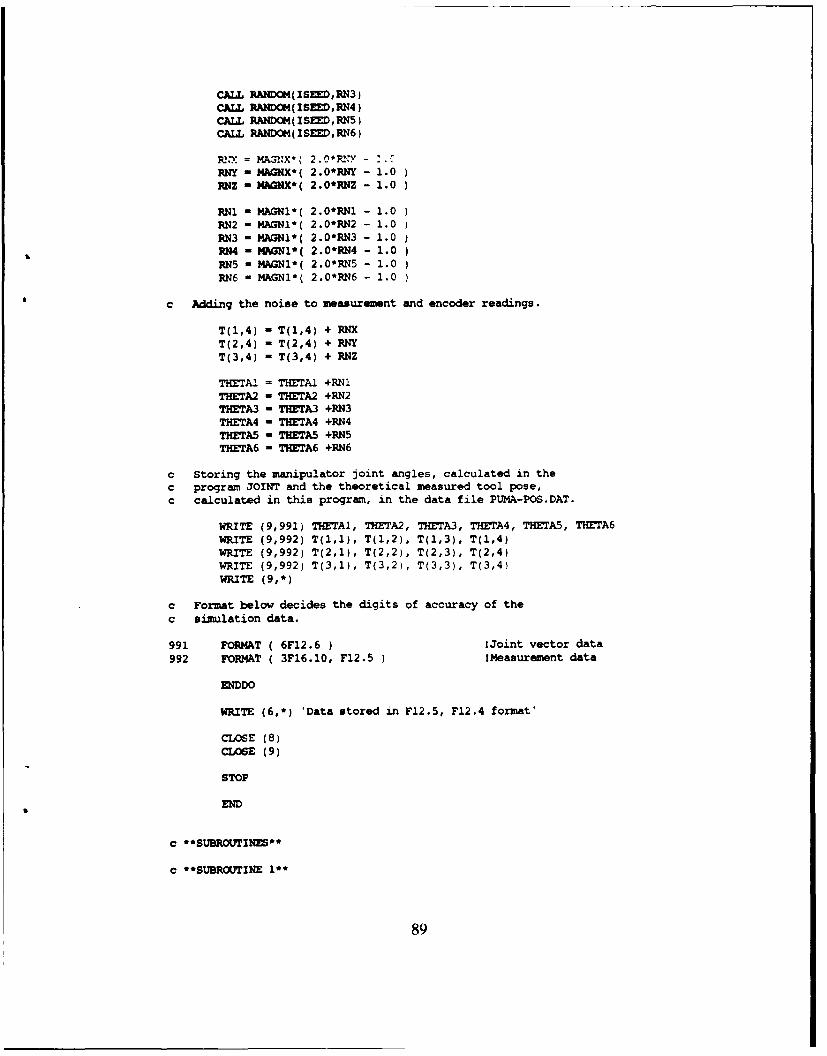
CALL RANDI(ISEED, RN3)CALL RANDOM( ISEED,RN4)CALL RANDOM( ISEED,RN5)CALL RANDOM(ISEED,RN6)

R-X = MA:X*( 2.0RhY -*RNY - MAGNX*( 2.0*RNY - 1.0

RNZ - MAGMX*( 2.0*RNZ - 1.0

RN1 - MAGN*( 2.0*RN1 - 1.0

RN2 - MAGNI( 2.0*RN2 - 1.0

RN3 - MAGN1*( 2.0*RN3 - 1.0RN4 - MAGN*( 2.0*RN4 - 1.0RN5 - MAGN1*( 2.0*RN5 - 1.0RN6 - MAGN1*( 2.0*RN6 - 1.0

c Adding the noise to measurement and encoder readings.

T(1,4) - T(1,4) + RNXT(2,4) - T(2,4) + RNYT(3,4) - T(3,4) + RNZ

THE:TAI = THETA1 +RNlTHETA2 - THETA2 +RN2THETA3 - THETA3 +RN3THETA4 - THETA4 +RN4THETA5 - THETA5 +RN5THETA6 - THETA6 +RN6

c Storing the manipulator joint angles, calculated in thec program JOINT and the theoretical measured tool pose,c calculated in this program, in the data file PUMA-POS.DAT.

WRITE (9,991) THETAI, THETA2, THETA3, THETA4, THETA5, THETA6WRITE (9,992) T(1,1), T(1,2). T(1,3), T(1,4)WRITE (9,992) T(2,1), T(2,2), T(2,3), T(2,4)

WRITE (9,992) T(3,1), T(3,2), T(3,3), T(3,4)WRITE (9,*)

c Format below decides the digits of accuracy of thec simulation data.

991 FORMAT ( 6F12.6 ) lJoint vector data992 FORMAT ( 3F16.10, F12.5 ) IMeasurement data

ENDDO

WRITE (6,*) 'Data stored in F12.5, F12.4 format'

CLOSE (8)CLOSE (9)

STOP

END

" **SUBROUTINES**

" **SUBROUTINE 1"*

89

SUBROUTINE RANDOM (X,Z)

REAL FM, FX, ZINTEGER A, X, I, MDATA ,

IF ( I .EQ. 0 ) GO TO 10001-01H= 2 ** 20FM- MA- 2**1O + 3

1000 X= MOD( A*X ,M)FX= XZ- FX/ FM

RETURN

END

90

APPENDIX E PROGRAM 1D6

PROGRAM ID6

c This is the pro-gram which identifies the kinematic parametersc of the simulated PUMA 560 manipulator using the Non-linear

b c Least Squares method in IMSL routine ZXSSQ using function" PUMAARM. The simulated poses are read from the data file" PUMA-POS.DAT

INI'MER LDFJAC, MM, M, NN, N~, NSIG, MAXFN, IOPT, IXJAC, INFER, IERINTEGER I, J, K, NOBS, MAXOBOS

REAL-8 FJAC(LDFJAC,NN), X3TJ( (NN+l) *NN/2)REAL-B PARM(4), F(LDFJAC), WORK((5*NN)+(2-MM.)+((NN+l)*NN/2flREAL*8 DANGLE, DLENTH, TQ, DQ, EPS, DELTA, SSQ, SQERR:I, SQER.2REAL*8 FIO, THO, 510, PXO, PYO, PZOREAL*8 DTl, DT2, DT3, DT4, DT5REAL*8 DDl, DD2, DD3, DD4, DD5REAL*8 AM1 AA2, AA3, AA4, AA5REAL*8 ALl, AL2, AL3, AL4, AL5REAL*8 BLl, BL2, BL3, BL4, BL5REL* DF6, TH6, S16, PX6, PY6, PZ6, F16REAL*8 TETi (MNOOBS), TET2 (MAXG4OBS), TET3 (MAXaNOBS)REL* TET4 (MAXG4OBSj, TET5 (MA)ONOBS), TET6 (MAXNOBS)REAL*a TM(3,4,MAXOBS), SCALE, X(NN)

PARAMETER (LDFJAC-6*36O, MM-LDFJAC, NN-30)

PARAMETER (MAXOIOBS=360)

EXTERNAL PUMA-ARM

COMMON /PDATA/ NOBS, TM, SCALE,

& TET1, TET2, TET3, TET4, TET5, TET6

c open data file for storage of output. This will be the identified" kinematic parameters.

OPEN (8, NAME-'RESULT.DAT, STATUS-'NEW')

" Open data file for the simulated poses. These were generated in" programi POSE.

OPEN (9, NAME- PUMA-POS .DAT*, STATUS- 'OLD-

c open data file of nominal kinematic parameters.

OPEN (10,NAME- INPUT.DAT', STATUS-'OLD-)

c Read nominal kinematic parameters from INPUT.*DAT.

read (10,*)read (l0,*) fiO,thO,si0,pxO,pyO,pzOread (10,*) dtl,ddl,aal,all,bllread (10,*) dt2,dd2,aa2,al2,b12

91

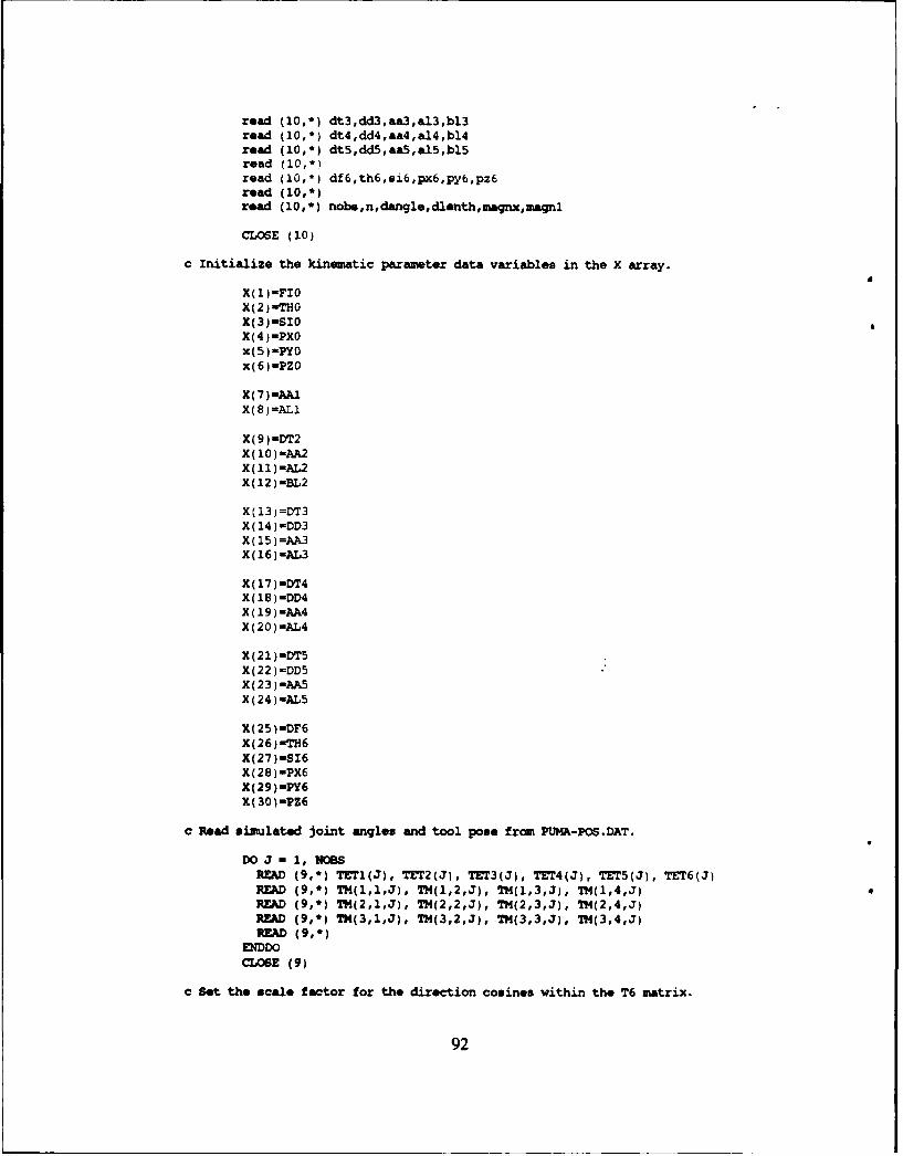
read (10,-) dt3,dd3,aa3,a13,b13read (10,*) dt4,dd4,aa4,a14,bl4read (10,') dt5,dd5,aa5,a15,b15read (10,*iread (10,*) df6,th6,si.6,px6,py6,pz6read (10,*)road (10,*) nobs,n,dangl.,dlenth,magnx,magnl

CLOSE (10)

c Initialize the kinematic parameter data variables in the X array.

X(1 )-FIX(2)-THOX(3)-SIOX(4)-PXOx (5) mPYOx(6)-PZO

X (7) -AA1X(8)=ALI

X( 9)-DT2X (10)-AA2X (11 )-AL2X(12)-BL2

X(13)=DT3X (14) -DP3XC 15) =AA3X (16)-AL3

X(17)-DT4X (18) -DD4X (19 =AA4X (20) AL4

X (21 ) DTSX(22)-D5X (23)-Ah5X (24) mAL5

X(25)-DF6X (26)-TH6X(27)-SI6X(28)-PX6X(29)-PY6X( 30)-PZ6

c Read simulated joint angles and tool pose from PUMA-POS .DAT.

DO J - 1, NOBSREAD (9'-) TET1(J), TET2(J), TET3(J), TET4(J), TET5(J), TET6(J)READ (9,') TM(1,1,J), TM(l,2,J), TM(1,3,J), TM(1,4,J)READ (9,') Th(2,1,J), TM(2,2,J), TM(2,3,J), 7M(2,4,J)READ (9,') Th(3,l,J), TM(3,2,J), Th(3,3,J), TM(3,4,J)READ (9,')

ENDDOCLIOSE (9)

" Set the scale factor for the direction cosines within the T6 matrix.

92

SCALEOO 0.0

" The following lines set the parameters necessary for the operationo of the IMSL routine, ZXSSQ, for identification of the kinematicC parameters.

o The subroutine which ZXSSQ is calling is PUMA_ARM.

NSIG-4EPS-0.0DELTA-0.0

* MA)CN:I500IOPT-lIXJAC-LDFJACH-6*NOBS

CALL ZXSSQ(PUMA _ARM,M,N,NSIG,EPS,DELTA,MAXFN, IOPT,& PARM,X,SSQ,F,FJAC,IXJAC,XJTJ,WORK, INFER, IER)

" Save identified kinematic parameters to data file RESULT.DAT.

WRITE (8,*)WRITE (8,*) 'FI0, THO, SI0, PXO, PYO, PZ0'WRITE (8,888) X(1), X(2), X(3), X(4), x(5), x(6)WRITE (8,*)WRITE (8,*) 'DT1, DD1, AAM, ALl, BLi'WRITE (8,888) 0.0, 0.0, X(7), X(8), 0.0WRITE (8,*)WRITE (8,*) 'DT2, DD2, AA2, AL2, BL2'WRITE (8,888) X(9), 0.0, X(10), X(11), X(12)WRITE (8,*)WRITE (8,*) 'DT3, DD3, AA3, AL3, BL3'WRITE (8,888) X(13), X(14), X(15), X(16), 0.0WRITE (8,*)WRITE (8,*) 'DT4, DD4, AA4, AL4, BL4'WRITE (8,888) X(17), X(18), X(19), X(20), 0.0WRITE (8,*)WRITE (8,*) 'DT5, DD5, AA5, AL5, BL5'WRITE (8,888) X(21), X(22), X(23), X(24), 0.0WRITE (8,*)WRITE (8,*) 'DF6, TH6, S16, PX6, PY6, PZ6'WRITE (8,889) X(25), X(26), X(27), X(28), X(29), X(30)

888 FORMAT ( 5F12.5889 FORMAT ( 6F12.5

" Calculate the root mean square error in identification of thec direction cosine and position parameters.

TQ - DANGLEDQ - DLENTH

" This calculates the error in identification of the directionc cosine parameters.

SQERR1 -& (FIO+TQ-X(l))**2+(TH0+TQ-X(2))**2+(SIO+TQ-X(3))**2& +(AL+TQ-X(8))**2+(DT2+TQ-X(9))**2+(AL2+TQ-X(lI))**2& +(BL2+TQ-X(12))**2+(DT3+TQ-X(13))**2+(AL3+TQ-X(16))**2& +(DT4+TQ-X(17) )**2+(AL4+TQ-X(20) )**2

93

&. +(DT5+TQ-X(21) )-2+(AL5+TQ-X(24) )*2

& +(DF6+TQ-X(25))**2+CTH6+TQ--X(26H"*2+(SI6+TQ-X(27fl"*2

SQER.1 - DSQRT( SQERl1/16

c This calculates the error in identification of the position" paramisters.

SQER.2& (PXO+DQ-X(4))**2+(FYO+DQ-X(5))**2+(PZO+DQ-X(6))-*2& *(AAl+DQ-X(7fl"*2+(AA2+DQ-X(1O))**2+(D03+DQ-X(l4))**2& +(AA3+DQ-X(15))**2+(DD4+DQ-X(18))**2+(AA4+DQ-X(19))**2& +(DD5+DQ-X(22) )-2+(A5+DQ-X(23) )"2& +(PX6+DQ-X(28))**2+(PY6+DQ-X(29))**2+(PZ6+DQ-X(30fl"*2

SQERR2 - DSQRT( SQERR2/14

c Write the position and orientation error to the data file" RESULT.DAT.

WRITE (8,')WRITE (8,') 'RHS PARMS (LENGTH), RMS PARMS (ANGLE)'WRITE (8,') SQERR2, SQERR1

" Write the position and orientation error to the screen.

WRITE (6,') 'RMS PARMS (LENGTH), RMS PARMS (ANGLE)'WRITE (6,') SQERR2,SQERR1

c Write the ZXSSQ convergence criteria to the data filec RESULT.DAT.

WRITE (8,')WRITE (9,*) 'INFER, IER, NOBS, NSIG'WRITE (8,') INFER, ZER, NOBS, NSIGWRITE (8,')

c Write the ZXSSQ convergence criteria to the screen.

WRITE (6,*) *INFIER, IER, NOSS, NSIG'WRITE (6,') INFER, IER, NOBS, NSIG

CLOSE (8)

END

" *URUIE*

" "SUBROUTINE 1"*

SUBROUTINE PUMh ARM (X, M, N, F)

" This subroutine calculates the non-linear function for the use ofc the IML routine ZXSSQ. It is the forward kinamatic solution forc the PUMA manipulator.

INTEGER M, N, 11, JJINTEGER 1, J, K, NOBS, MAJOIOBS

REAL'8 X(N)v F(M)REAL'8 FIO, THO, SIO, PXO, PYO, PZOREAL'S DT1, DT2, DT3, DT4, DT5

94

PEAL*8 DDl, DD2, DD3, DD4, DD5ilEAL*8 AJU, AA2, AA3, AM4, AA5REAL*8 AL1, AL2, AL3, AL4, AL5REA'!*P ELI, BL2, BL?, BL4, BicREAL*8 F16, TH6, S16, PX6, PY6, PZ6, DF6REAL*8 Till, TH2, TH3, TH4, TH5RERL*8 TO(4,4), Tl(4,4), T2(4,4), T3(4,4), T4(4,4)REAL*B T5(4,4), T6(4,4), TRPY(4,4), TXYZ(4,4)REAL*8 TIMAT(4,4), T(4,4)REAL-8 TINV(4,4), TMJ3(4,4), TDELTA(4,4)REAL-8 TETi (MAXNOBS), TET2 (MA)[NOBS), TET3 (MAXGNOBS)

* RAL*8 TET4 (MAXO4OBS), TET5 (MAXNOBS), TF'6 (MAXNOES)pEAL*8 TM(3,4,MAXNOBS), SCALE

* PARAMETER (MAXNOES-360)

COMMO4N /PDATA/ NOBS, TM, SCALE,

& TETi, TET2, TET3, TET4, TET5, TET6

"Initializing the TIMAT matrix to an identity matrix.

DATA TIMAT/1,O,0,0,0,1,0,0,O,0,1,0,0,O,O, 1/

" Assign kinematic parameters to the variable X array.

FIO = X(1)THO - X(2)SIO = X(3)PXO - X(4)PYO = x(5)PZO -x(6)

DTl - 0.0DDl - 0.0AA1 = X(7)ALl - X(8)ELi - 0.0

DT2 - X(9)DD2 = 0.0AA2 - X(10)AL2 - X(11)BL2 - X(12)

DT3 -X(13)DD3 - X(14)AA3 - X(15)AL3 - X(16)91.3 - 0.0

DT4 - X(17)DD4 - X(18)AU - X(19)AL4 -X(20)91.4 - 0.0

DT5 - X(21)DD5 - X(22)AA5 - X(23)AL5 - X(24)31.5 - 0.0

95

DF6 - X(25)TH6 - X(26)S16 = X(27)PX6 - X 26)PY6 - X(29)PZ6 X(30)

c Loop through NOBS times.

K-0DO J - 1, NOBS 0

c Initializing the T matrix to an identity mtrix.

DO II - 1,4DO JJ = 1,4T(II,JJ) - TIMAT(II,JJ)ENDDOEDDO

c Calculate the actual manipulator joint angles.

TH1 - DT1 + TETl(J)TH2 = DT2 + TET2(J)TH3 = DT3 + TET3(J)TH4 - DT4 + TET4(J)TH5 = DT5 + TET5(J)F16 - DF6 + TET6(J)

c Compute the T matrices, TI thru T6.

CALL T3RPY( FIO, THO, SI0, TRPYCALL T3XYZ( PXO, PYO, PZO, TXYZCALL MATMULC( TO, TRPY, TXYZ )

CALL TRANSFORM ( ALl, AA1, DDl, THI, BL1, TiCALL TRANSFORM ( AL2, AA2, DD2, TH2, BL2, T2CALL TRANSFORM ( AL3, AA3, DD3, TH3, BL3, T3CALL TRANSFORM ( AL4, AA4, DD4, TH4, BL4, T4CALL TRANSFORM ( AL5, AA5, DD5, TH5, BL5, T5

CALL T3RPY( FI6, TH6, S16, TRPYCALL T3XYZ( PX6, PY6, PZ6, TXYZCALL MATMULC(T6, TRPY, TXYZ )

" Compute the complete transformation from the base frame to" the tool frame.

CALL MATMULA ( T, TOCALL MATMULA ( T, TiCALL MATMULA ( T, T2CALL MATMULA ( T, T3CALL MATMULA (T, T4CALL MATMULA ( T, T5CALL MATMULA ( T, T6

c Read the simulated measured T matrix for this observation:

DO II 1,3

DO JJ - 1,4

96

TI4J(IIJJ) - T?4(IIJJJ)

ENDDOENDO

c Remember that row 4 is 0, 0, 0, 1.

TMJ(4,l) - 0.0TMJ(4,2) - 0.0TKJ(4,3) - 0.0

do c Compute the difference between the measured T matrix and the

c T matrix generated using the latest table of kinematic data.

CALL MATSUB ( TDELTA, TMJ, T)

c Calculate the function F (six rows at a time).

o First, position.

F = K+ 1F(K) = TDELTA(1,4)K-K +l1F(K) =TDEL.TA(2,4)T,= K+l1F(K) =TDELTA(3,4)

c Now orientation.

K = K+ 1F(K)- ((TDELTA(3t2)-TD.LTA(2,3))/2.0) * SCALEK-K + 1F(K) -((TDELTA(l,3)-TDETA(3,l))/2.0) *SCALEK-K + 1F(Y) = ((TDELTA(2,1)-TDELTA(l,2))/2.0) * SCALE

c Ending the DO loop f or J counter.

ENDDO

c Write PJMS error in function F.

xSSQ=0.0

DO II-1,6NOBSXSSQ=XSSQ+F(II) *F(II)

WNDDO

XER-SQRT (XSSQ)

c Write RMS error to the screen. This allows the operator

c to track how the identification process is proceeding.

WRITE(6,*) E

RETURN

END

97

APPENDIX F PROGRAM VERIFY

PROGRAM VERIFY

C This program generates the six-dof pose error for the PUMA manipulator.C It contains the identified calibration parameters and the exact parameter.C It uses a data file of verification joint angle sets POSEVER.DAT, and theC file RESULT.DAT from the program 1D6.e

INTEGER I, J, K, NPOSL:, N, nobREAL* 8 DAN GLE , DENTH

REAL*8 DT(5),dd(5),aa(5),al(5),bl(5)REAL*8 eDT(5) ,edd(5) ,eaa(5) ,eal(5) ,ebl(5)REAL*8 edf6, EF16, ETH6, ESI6, EPX6, EPY6, EPZ6REAL*8 EDFO, EFIO, ETHO, ESIG, EPXO, EP60, EPZOREAL*8 THETA(1000,6), TDELTA(4,4J

REAL*8 T4(4,4), T5(4,4), T6(4,4), TRPY(4,4), TXYZ(4,4)

REAL*8 TIMAT(4,4), T(4,4), et(4,4)

pRJ.L*8 DFO, DTO, DSO, PXO, PY0, PZ0RE&L*8 DT1, DT2, DT3, DT4, DT5REAL*8 DDI, DD2, DD3, DD4, D05REAL*8 AM1, AA2, AA3, AM, AM5REL* ALI, AL2, AL3, AL4, AL.5

REAL*8 BLI, BL2, BL3, BL4, BL5

REAL*8 DF6, DT6, DS6, PX6, PY6, PZ6

COM40N TIMATTTI'A

EXTERNAL FKS

C Initialize the TIMAT matrix to an I matrix:

DATA TIMAT/l,0,0,0,0, 1,0, 0,0,0,1,0,0,0,0,1/

C Open data file

OPEN (9, NAE-'posever.DAT,STATUSOLD')OPEN (10, NAME='input.DAT', STATUS-'OLD')OPEN (11, NAE=result.DAT', STATUS-'OLD')open (12, name'rror.dat',aecess-'append',status-unknown')

c Read input parameters

read (l0,*)read (lO,*) dfO,dtO,dsO,pxO,pyO,pzOread (l0,*) dtl,ddl,aal,all,bll

read (10,*) dt2,dd2,aa2,al2,b12read (10,*) dt3,dd3,aa3,a13,b13read (1O,*) dt4,dd4,aa4,a14,b14read (10,*) dt5,ddS,aa5,a15,b15road (lO,*)read (l0,*) df6,dt6,ds6,px6,py6,pz6read (10,*)

98

read (10,*) nobs,n,dangle,dlenth,magnx,magnl

CLOSE (10)

c Read in joint angle sets for verification poses

do i=l,nobsread(9,*)theta(i,l),theta(i,2),theta(i,3),theta(i,4),

theta(i,5),theta(i,6)enddoclose (9)

C Set exact link parameters for the manipulator:

DT(l)-0.0do i=2,5

dt(i)=dangleenddo

DFO = DFO + DangleDTO = DTO + DANGLEDSO = DSO + DANGLEPXO = PXO + DLENTHPY0 = PYO + DLENTHPZO = PZO + DLENTH

al(l) = all + DANGLEal(2) = a12 + DANGLEal(3) = a13 + DANGLEal(4) = a14 + DANGLEal(5) - a15 + DANGLE

AA(l) = aal + DLENTHAA(2) = aa2 + DLENTHAA(3) - aa3 + DLENTHAA(4) = aa4 + DLENTHAA(5) = aa5 + DLENTH

DD(l) - ddl I definedDD(2) - dd2 I definedDD(3) - dd3 + DLENTHDD(4) = dd4 + DLENTHDD(5) - dd5 + DLENTH

BL(l) - bll I definedBL(2) = b12 + DANGLEBL(3) = b13 I definedBL(4) - b14 I definedBL(5) - b15 I defined

DF6 - DF6 + DangleDT6 - DT6 + DANGLEDS6 - DS6 + DANGLEPX6 - PX6 + DLENTHPY6 - PY6 + DLENTHPZ6 - PZ6 + DLENTH

c Read in and set up estimated parameter table

99

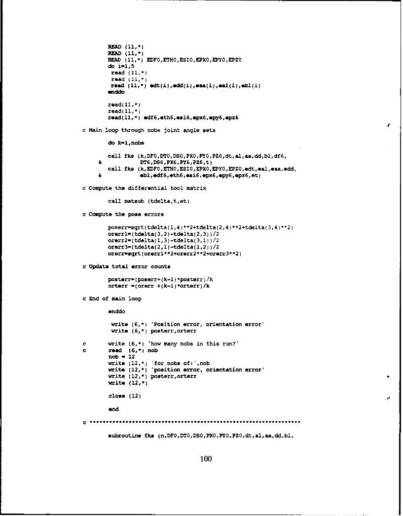
READ (11,)READ (11,*READ (ll,*) EDFO,ETHO,ESIO,EPXO,EPYO,EPZOdo i-1,5read (ll,*)read (11,*)read (1l,*) .dt(i),edd(ibaa(iJ,eal(i),.bl(i)

.nddo

read( 1, *)read( 11,*read(ll,*) edf6,eth6,esi6,epx6,*py6,epz6

c Main ioop through nobs joint angle sets

do k-l,nobe

call fks (k,DFO,DTO,DSO,PXO,YO,PZO,dt,al,aa,dd,bl,df6,& DT6,DS6,PX6,PY6,PZ6,t)call fka (k,EDFO,ETHO,ESIO,EPXO,EPYO,EPZO,edt,eal,eaa,edd,& ebl,edf6,eth6,esi6,epx6,epy6,epz6,et)

c Compute the differential tool matrix

call matsub (tdelta,t,et)

c Compute the pose errors

poserr-sqrt(tdelta(,4)**2+tdelta(2,4)**2+tdelta(3,4)**2)orerrl=(tdelta(3,2)-tdelta(2,3) )/2orerr2=(tdelta(l,3)-tdelta(3,l) )/2orerr3-(tdelta(2,l)-tdelta(l,2) )/2orerrmsqrt (orerrl**2+orerr2**2+orerr3**2)

c Update total error counts

posterr= (poserr+ (k-l )*posterr) 1korterr =(orerr +(k-l)*orterr)/k

c End of main loop

enddo,

write (6,*) 'Position error, orientation error'write (6,*) posterr,orterr

c write (6,*) 'how many mobs in this run?'C read (6,*) nob

mob - 12write (12,*) 'for mobs; of:',nobwrite C12,*) 'position error, orientation error'write (12,*) posterr,orterrwrite (12,*)

close (12)

end

c

subroutine fks (n,DFO,DTO,DSO,PXO,PYO,PZO,dt,al,aa,dd,bl,

100

df6,th6,si6,px6,py6,pz6,t)

REAL-8 TO(4,4), Ti(4,4), T2(4,4), T3(4,4)

REAL*B T4(4,4), T5(4,4), T6(4,4), TRPY(4,4), TXYZ(4,4jREAL*8 TIMAT(4,4), T(4,4). dt(5) ,al(5) ,aa(5) ,dd(5) ,bl(5)

re.a18 theta(1OOO,6), ang(6)c~n timat, theta

C Initialize the T matrix to an I matrix.

DO J-1,4DoK-1,4

T(J,K) - TIMAT(J,K)ENDDOENDDO

C Set up joint angles

do i-1,5ang(i)-theta(l,i)+dt(i)enddo

fi6-df6+theta(n, 6)

C Compute the T matrices, Ti thru T6:

CALL T3RPY (DFO,DTO,DSO,TRPY

CALL T3XYZ (pxO,pyO,pzO,TXYZCALL MATMULC ( TO, TRPY, TXYZ

CALL TRANSFORM (al(l),aa(l) ,dd(l),ang(l),bi(l),Tl)CALL TRANSFORM (ai(2),aa(2),dcf(2),ang(2),bl(2),T2)CALL TRANSFORM (al(3),aa(3),dd(3),ang(3),bl(3),T3)CALL TRANSFORM (al(4) ,aa(4) ,dd(4) ,ang(4) ,bl(4) ,T4)

CALL TRANSFORM (al(5) ,aa(5) ,dd(5) ,ang(5) ,bl(5) ,T5)

CALL T3RPY (fi6,th6,si6,TRPYCALL T3XYZ (px6,py6,pz6,TXYZCALL HATWULC (T6, TRPY, TXYZ

C Compute the overall transformation, T:

CALL MATMULA (T, TOCALL MATHULA T, TiCALL KPATMULA (T, T2CALL MhTMULA (T, T3CALL MAThULA (T, T4CALL MATMULA (T, T5CALL MATMULA (T, T6

returnend

101

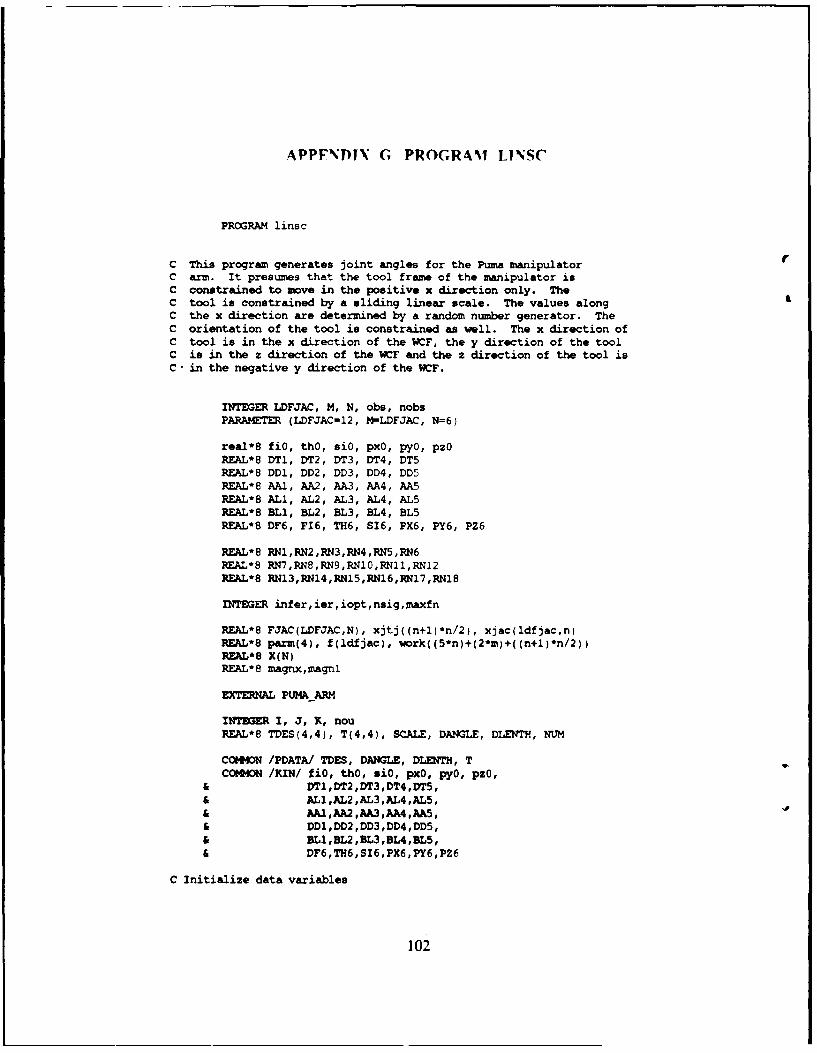
APPFNT)IN G PROGRAM LINSC

PROGRAM linsc

C This program generates joint angles for the Puma manipulator rC arm. It presumes that the tool frame of the manipulator isC constrained to move in the positive x direction only. TheC tool is constrained by a sliding linear scale. The values alongC the x direction are determined by a random number generator. TheC orientation of the tool is constrained as well. The x direction ofC tool is in the x direction of the WCF, the y direction of the toolC is in the z direction of the WCF and the z direction of the tool isC- in the negative y direction of the WCF.

INTEGER LDFJAC, M, N, obs, nobsPARAMETER (LDFJAC=12, M=-LDFJAC, N=6)

real*8 fiG, thO, siG, px0, pyO, pz0REAL*8 DTl, DT2, DT3, DT4, DT5REAL-8 DDl, DD2, DD3, DD4, DD5REAL*8 AAI, A&2, AA3, AA4, AA5REAL-8 ALl, AL2, ,AL3, AL4, AL5REAL*8 BLl, BL2, BL3, BL4, BL5REAL*8 DF6, F16, THE, S16, PX6, PY6, PZ6

REAL*8 RNl,RN2 ,RN3,Rk44,RN5,RN6REAL*8 R7,RN8,RN9,RNlO,RNll,RNI2REAL*8 RN13,RNl4,RNl5,RNl6,Rl7,R~l8

INTEGER infer,ier,iopt,nsig,maxfn

REAL*8 FJAC(LDFJAC,N), xjtj((n+l)*n/2), xjac(ldfjac,n)REAL*8 parm(4), f(ldfjac), work((5*n)+(2*m)+C(n+l)*n/2))REW*8 X(N)REAL*8 magnx,magnl

EXTERNAL PUMA-ARM

fITEGER1~ , J, K, nouREAL*8 TDES(4,4), T(4,4), SCALE, DANGLE, DLENTH, NUM

COMMON /PDATA/ TDES, DANGLE, DLENTN, TCOMMO0N /KINh/ fiG, thO, siG, px0, pyG, pz;0,

& DT1,DT2,DT3,DT4,VT5,& AL1,AL2,AL3,AL4,AL5,& AAl,AA2,AA3,AA4,Ah5,& DD1,DD2,DD3,DD4,DD5,& BL1,BL2,BL3,BL4,3L5,& DF6,TH6,SI6,PX6,PY6,PZ6

C Initialize data variables

102

obs-O

C Open data files for input

OPEN (IC, N!T='pmra-pc s.d*, STATUS '"EWOPEN (9, NAME-'input.dat', STATUS='OLD')

C Read input kinematic data

read (9,')read (9,') fiO,thO,siO,pxO,pyO,pzGread (9,') dtl,ddl,aal,all,bllread (9,') dt2,dd2,aa2,al2,bl2read (9,') dt3,dd3,aa3,a13,b13read (9,') dt4,dd4,aa4,al4,b14read (9,') dt5,dd5,aa5,a15,bl5read (9,')read (9,') df6,th6,si6,px6,py6,pz6read (9,')read (9,') nobs,nou,dangle,dlenth,magnx,magnl

close (9)

C Adjust nominal values

fiO=fiO+danglethO-thO+danglesiO-siO+danglepxO-pxO+dlenthpyO=pyO4-dlenthpzO-pzO+dlenth

dtl-O.Odt2-dt2+dangledt3-dt3+dangledt4-dt4+dangledt5-dt5+dangle

allu-all+danglea1l2-al2+danglea13-al3+dangleal4-a14+dangleal5=al54dangle

aal-aal+dlenthaa2=aa2+dlenthaa3-a&3+dlenthaa4=aa4+dlentha5-aa5+dlenth

ddlinO.0dd2-O.Odd3-dd3+dlenthdd4-dd4+dlenthdd5-dd5+dlenth

bli-blibl2-bl2+danqlebl3inbl3bl4Ubl4

103

bl5-bl5

df6-df6+dangleth6th6+dangle

c si6-i6+danglec px6-px6+dlerithc py6-py6dlenthc pz6-pz6+dlenth

C Get random number seed

write (6, *1 'Type in a 6-digit random number seed'

read (5,*) iseed

C Start of main loop

1010 cbuinobe+1

C Set joint angles to zero

do i=1,nx(i)0O.0.nddo

C Get random bar angles

1000 call random (iseed,nwn)nium-=rum*900 .0

C Establish desired tool pose

do ii-l,4do jj-l,4

TDES(ii,jj )0.0enddoenddo

TDES(l,4)- numTDES(4,4)- 1.0TPES(l,1)- 1.0TDES(3,2)- 1.0TDES(2,3)- -1.0

C Call IMSL ZXSSQ for inverse kinematic solution

nsig-4eps- 0.0

delta-0.0maxfnn500iopt-1ixjac-ldfjac

CALL ZXSSQ(puma_armn,m,n,nsig,eps,delta,maxfn,iopt,parnlx,ma,f,xjac,ixjac,xjtj,work,infer,ier)

C Check for singrularities

if (ssq Cgt. 0.00001) goto 1000

C Print results to 2 decimal places

104

write(6,*) obs,ssq

C Generate the random noise

CALL RAN-K*V. (IsE,:"CALL RANDOM (ISEED,RN2)CALL RANDOM (ISEED,RN3)CALL RANDOM (ISEED,RN4)CALL RANDOM (ISEED,RNS)CALL RANDOM (ISEED,RN6)CALL RANDOM (ISEED,RN7)CALL RANDOM (ISM,RN8)CALL RANDOM (ISEED,RN9)CALL RANDOM (ISEED,RNI0)CALL RANDOM (ISEED,RN11)CALL RANDOM (ISEE,RN12)CALL RANDOM (ISEED,RN13)CALL RANDOM (ISEED,RN14)CALL RANDOM (ISEED,RN15)CALL RANDOM (ISEED,RN16)CALL RANDOM (ISEED,RN17)CALL RANDOM (ISEED,RN!8)

RN1 - MAGNX * (2.0 * RN1 - 1.0)RN2 = MAGNX * (2.0 RN2 - 1.0)

RN3 MAGNX* (2.0 * RN3 - 1.0)

RN4 = MAGN1 * (2.0 * RN4 - 1.0)

RN5 = MAGNi * (2.0 * RN5 - 1.0)

RN6 = MAGN1 * (2.0 * RN6 - 1.0)

RN7 = MAGNI * (2.0 * RN7 - 1.0)

RN8 - MAGN1 * (2.0 * RN8 - 1.0)

RN9 - MAGNI * (2.0 * RN9 - 1.0)

RN10 = MAGN1 * (2.0 * RN10 - 1.0)

RN11 - MAGN1 * (2.0 * RN11 - 1.0)RN12 = MAGN1 * (2.0 * RN12 - 1.0)RN13 - MAGNI * (2.0 * RN13 - 1.0)

RN14 - MAGN1 * (2.0 * RN14 - 1.0)RN15 - MAGNI * (2.0 * RN15 - 1.0)RN16 - MAGN1 * (2.0 * RN16 - 1.0)

RN17 = MAGN1 * (2.0 * RN17 - 1.0)

RN18 - MAGN1 * (2.0 * RN18 - 1.0)

T(1,4) = T(1,4) + RN1T(2,4) - T(2,4) + RN2T(3,4) - T(3,4) + RN3

T(1,1) - T(1,1) + RN4T(1,2) = T(1,2) + RN5T(1,3) - T(1,3) + RN6

T(2,1) - T(2,1) + RN7T(2,2) - T(2,2) + RN8T(2,3) - T(2,3) + RN9

T(3,1) - T(3,1) + RN10T(3,2) - T(3,2) + RN11T(3,3) - T(3,3) + RN12

X(1) - X(1) + RN13X(2) - X(2) + RN14

105

X(3) - X(3) + RN15X(4) - X(4) + RN~16X(5) - X(5) + RN17X(6) - X(6) + RN18

write (10,0) X(l) ,X(2 J X(3) ,X(4) ,X(51 ,X(6)write (10.')write (10,') T(l,l),T(l,2),T(1,3bT(l,4)write (10,') T(2,l) ,T(2,2) ,T(2,3),T(2,4)write (10,') T(3,l) ,T(3,2) ,T(3,3),T(3,4)write (10,')

991 FORMAT (6F12.6 (992 FORMAT (3F16.10, F12.5

C Continue f or other bar angles

if (obs .1t. nobs) go to 1010

COSE (10)

END

C .*******************************

SUBROUTINE PUMAARM (X,M,N,F)

C This subroutine calculates the non-linear function for the use ofC the IML routine ZXSSQ. It is the forward kinematic solution forC the PUMA manipulator.

INTEGER M, NREAL'S Xcii), F(M)

INTEGER II, JJreal*S fi0, tho, si0, px0, pyO, pzaREAL'S DT1, DT2, DT3, DT4, DT5REAL'8 DD1, DD2, DD3, DD4, DD5REAL'S AA1, AA2, AA3, AA4, AMBREAL*S ALl, AL2, AL3, AL4, AL5REAL*8 BLi, DL2, BL3, BL4, BLj5REAL'S DF6, F16, TH6, S16, PX6, PY6, PZ6

REAL'S Till, TH2, TH3, TH4, TH5REAL*S TO(4,4), Tl(4,4), T2(4,4), T3(4,4), T4(4,4)REAL'S T5(4,4), T6(4,4), trpy(4,4), txyz(4,4)REAL'S TIMhT(4,4), T(4,4), td(4,4)

INTEGER 1, J, KREAL'S TDES(4,4), DANGLE, DLE2ITH,scale

COMMON /PDATA/ TDES, DANGLE, DLENTH, T4COMMON /KIN/ fiO,th0,siOpxO,pyO,pzO,

& DT1,DT2,DT3,DT4,DT5,& ALl,AL2,AL3,AL4,AL5,& AAl,AA2,AA3,AA4,AA5,& DD1,DD2,DD3,DD4,DD5,& DL1,BL2,BL3,BL4,BL5,& DF6,TH6,SI6,PX6,PY6,PZ6

C Initialize the TIMAT matrix to an I matrix:

106

DATA TIMAT/l,O,O,0, 0,1,0, 0,0, 0,1,0,0,0,0,1/

scale-100 .0

C Initialize the T matrix to an I matrix

DO 11 - 1,4DO) JJ - 1,4

T(II,JJ) = TIMAT(II,Jj)ENDDOENDDO

C Manipulator joint angles

TH1 - DT1 + X(1)TH2 - DT2 + X(2)TH3 - DT3 + X(3)TH4 - DT4 + X(4)TH5 - OTS + X(5)F16 - DF6 + X(6)

C Compute the T matrices, T1 thru T6:

call t3rpy (fi0,thO,si0, trpy)call t3xyz (px0,py0,pzO, txyz)call matznulc (tO,trpy,txyz)

CALL TRANSFORM (ALl, AJ2, DDl, THi, BLi, T1CALL TRANSFORM (AL2, AA2, DD2, TH2, BL2, T12CALL TRANSFORM ( L3, AA3, DD3, TH3, BL3, T3CALL TRANSFORM (AL4, AAM, DD4, TH4, BL4, T14CALL TRANSFORM (AL5, AA5, DD5, TH5, BL5, T15

CALL t3rpy (fi6, th6, si6, trpyCALL T3XYZ (PX6, PY6, PZ6, txyzCALL matmulc t6, trpy, txyz

C Compute the overall transformation, T1:

CALL MATMULA (T, TOCALL MATMULA (T, TiCALL MATMULA (T, T2CALL MATMULA (T, T3CALL MATMULA (T, T4CALL MATMULA (T, T15CALL MATMULA (T, T6

call matuub(td,tdes ,t)

C Calculate the function F

f (l1)-td (1,4)f(2)-td(2,4)f (3) -td (3,4)f(4)-td(1,1)*scalef(5)-td(1,2)*scalef(6)-td(1,3)*scalef(7)-td(2,1)*scalef(8)-td(2,2)*scalef(9)-td(2,3)*scale

107

f(10)-td(3,1)*scalef(11)-td(3,2)*scalef(12)-td(3,3)*scale

sum - 0.0do i-l,12xssq-sum+f(i)

enddoC write (6,*) xssq

RETURNEND 4

C ***...****************.e **** ******** *.************

SUBROUTINE RANDOM (x,z)

C This subroutine generates random numbers in the range 0-1C using a supplied seed x, the returned random number being z.

REAL FM, FX, ZINTEGER A, X, I, MDATA I/l/

IF ( I .EQ. 0 ) GO TO 1000I-0No 2 ** 20FM_ MA- 2*10 + 3

1000 X- MOD( A*X ,M)FX- XZ- FX/ FM

RETURNEND

108

APPENDIX H PROGRAM ACDAT

program acdat

C This program is the data acquisition program for the linearC slide version of the puzma manipulator calibration experiments.C It requirem that the value for the distance down the linearC slide and the six joint angles of the puma when it is in thatC configuration. The pose data is saved in the file "slide-pos.dat."C That file is set up in the append mode.

real*8 x, thl, th2, th3, th4, th5, th6real*8 tm(4,4)

open (10, name='slide-pos.dat',access='append',status='unknown')

C Inputting the distance down the linear slide.

100 write (6,*) 'input the value for x'read (6,*) x

C Inputting the six joint angles.

write (6,*) 'input the 6 joint angles'read (6,*J thl, th2, th3, th4, th5, th6

C This will set the T6 matrix for the value of x measured.

do ii-1,4do jj-l,4

tm(ii,jj )=0.0enddo

enddo

tm(1,4)= xtm(4,4)= 1.0tm(1,1)= 1.0t(3,2)- 1.0tm(2,3)" -1.0

C Writing the pose data to "slide-pos.dat"

write (10,991) thl, th2, th3, th4, th5, th6write (10,*)write (10,992) tm(1,1),tm(1,2),tm(1,3),tm(1,4)write (10,992) tm(2,1),tm(2,2),tm(2,3),tm(2,4)write (10,992) tm(3,1),tm(3,2),tm(3,3),tm(3,4)write (10,992) th(4,1),tm(4,2),tm(4,3),tm(4,4)write (10,*)

write (6,*)write (6,*) 'data saved'write (6,*)

109

write (6,*) 'do you wish to make another observation'write (6,*? 'enter a 1 for yes or a 0 for no'write (6,*)read (6,*) ane

if (an, .eq. 1) go to 100

991 FORMAT (U612.6992 FORMAT (3F16.10, F12.5

closeC 10)stop

end

110

APPENDIX I PROGRAM ID6-LINSC

PROGRAM ID6_LINSC

C Robot Identification using the Non-linear Least Squares method.C Simulation data is read for the PUMA manipulator from

-' C the data file PUMA-POS.DAT

C Change parameter LDFJAC to change the nu~mber of observations,C set WDFJAC - 6 * Numiber of observations

INTEGER LDFJAC, MM4, M, NN, N, NSIG, MAXFN, IOPT, IXJAC, INFER, IERPARAMETER (LDFJAC>l2 '42, MO4=LDFJAC, NN-2 6)

REAL*8 F3AC(LDFJAC,NN), XJTJ( (NN+l ) NN/2)pWE3,*8 PARM(4), F(LDFJAC), W0RK((5*NN)+(2-M)q1)+((NN+l)*NNI2))REA'8 X(NN)

EXTERNAL PUMAARM

REAL*8 DAN GLE , DLENTH, TQ, DQ, EPS, DEL~TA, SSQREAL*8 SQERR, SQERP.2

real*8 fiO,thO,si,pxO,pyO,pzOREAL*8 DTl, DT2, DT3, DT4, DT5REAL*S DD1, DD2, DD3, DD4, P05

PEAL'S AM., AA2, Ah3, AM4, AA5pRkTL*8 ALl, AL2, AL3, AL4, AL5

REAL*S BLI, BL2, BL3, BL4, BL5

REAL'S DF6, TH6, S16, PX6, PY6, PZ6, F16

INTEGER 1, J, K, NOBS, MA)X4OBSPARAMETER (MAXNOBS-36O)REAL'S TETi (MA)OIOBS), TET2 (MAXGbOBS), TET3 CMAXNOBS)REAL*8 TET4 (MAXOBOS), TEr5 (MAXONOBS), TET6 (MAXNOBS)

REAL'S TM(3,4,MAXNOBS), SCALECOMMON /PDATA/ NOBS, TM, SCALE,

& TET1, TET2, TET3, TET4, TET5, TET6

C open data files for inputs and results

OPEN (8, NAME-' RESULT .DAT', STATUS-'NEW')OPEN (9, NAME 'PUMA-POS .DAT*, STATUS- 'OLD')OPEN (10,NAME-'INPIYT.DAT', STATUS-'OLD')

c Read input parameters

read (10,')read (10,') fi0,th0,si0,pxc0,py0,pz0read (10,*) dtl,ddl,aal,all,bllread (10,') dt2,dd2,aa2,a12,b12read (10,') dt3,dd3,aa3,a13,b13road (10,') dt4,dd4,aa4,&14,bl4read (10,') dt5,dd5,aa5,a.15,bl5read (10,')

read (10,') df6,th6,si6,px6,py6,pz6

read (10, *)

read (10,*) nobs,n,dangle,dlenth,magnx,magni

CLOSE (10)

write (6,*) 'enter nobs'read (6,*) nob.

C Initialize data variables

X(l)=fi0X(2)-thOX(3)-siOX(4)-pxOx(5)-py0x(6).'PZO

X (7)-AMIX(8)-AL1

X (9) -DT2X (10) =AA2XC 11 )=AL2X(12)-BL2

XC 13) =DT3X(14)=DD3X( 15)-'AA3X(16)=AL3

X(17 )=DT4X (18) DD4X (19)-AA4XC 20) =AL4

X(2 )-DT5X(22)=DD5X (23) -AA5X(24)-AL5

x (25 )-df 6x(26)-th6

c x(27)-si6c x(28)-px6c x(29)=Wp6c x(30)-.pz6

C Read simulated joint data and tool pose

DO J - 1, NOBSREAD (9,-) TET1(J), TET2(J), TET3(J), TET4(J), TET5(J), TET6(J)road (9,*)

READ (9,*) TH(2,l,J), TM(1,2,J), TM(1,3,J), Th(2,4,J)READ (9,*) TM(2,l,J), TM(3,2,J), TM(23,J), TM(2,4,J)READ (9,*) T(,,) M32JT(,,) M34J

cREAD (9,*)

CLOSE (9)

C Initialize scale for the angular rows of the Jacobian

112

SCAL.E1l0.O0

C Call IMSL routine for non-linear identification

NS5IGin3EPS-o *

DELTA0. 0MAXFN=15 00IOPT~lIXJAC-LDFJAC

N M=12*NOBS

CALL ZXSSQ(PUA AM,M,N,NSIG,EPS,DELTA,MAXN,IOPT,& PARM,X,SSQ,F,FJAC,IXJAC,XJrJ,WORK,INF-ER,IER)

C Save results to data file

WRITE (8,*)WRITE (8,*) 'fiO, tho, ajo, pxo, pyo, pzo'WRITE (8,888) X(l), X(2), X(3), X(4), x(5), x(6)WRITE (8,*)WRITE (8,*) *DTl, DDl, AAM, ALl, BLiWRITE (8,888) 0.0, 0.0, X(7), X(8), 0.0WRITE (8,*)WRITE (8,*) 'DT2, DD2, AA2, AL2, BL2'WRITE (8,888) X(9), 0.0, X(10), X(11), X(12)WRITE (8,*)WRITE (8,*) 'DT3, DD3, AA3, AL3, BL3'WRITE (8,888) X(13), X(14), X(15), X(16), 0.0WRITE (8,*)WRITE (8,*) *DT4, DD4, AA4, AL4, BL4'WRITE (8,888) X(17), X(18), X(19), X(20), 0.0WRITE (8,*)WRITE (8,*) 'DT5, DD5, AA5, AL5, BL5'WRITE (8,888) X(21), X(22), X(23), X(24), 0.0WRITE (8,*)WRITE (8,*) 0DF6, TH6, S16, PX6, PY6, PZ6'WRITE (8,889) x(25),x(26), si6, px6, py6, pz6

888 FORMAT (5F12.5889 FORMAT (6F12.5

C Calculate root mean square error in identification

TQ - DA24GLDQ - DLENTH

C Error in identification (angular parameters)

SQERR1G (FIO+TQ-X(l))**2 +(THO+TQ-X(2) )*2 +(SI0+TQ.-X(3fl**2& +(DT34TQ-X(13))-*2 +(DT4+TQX(l7))-*2 +(DT54TQ-X(21))**2& +(AL1+TQ-X(8))**2 +(AL2+TQ-X(l))**2& +(AL3+TQX(16))**2 +(AL4+TQ-X(20))**2 +(AL5+TQ-X(24))**2& +(BL2+TQ-X(12))2 +(DT2+TQ-X(9).)**2& +(df6+tq-x(25) )**2 +(th6+tq-x(26) )**2

SQERR1 - DSQRT( SQERRl/15

C Error in identification (length parameters)

113

SQE=R =&(PXO+DQ-X(4fl**2 +(AAl+O.O+DQ-X(7))**2 *(AA2+DQ-X(10fl-2

& +(AA,3+DQ-X(15fl**2 +(AA4+DQ-X(l9fl**2 +(AA5+DQ-X(23fl'*2& +(PYO+DQ-X(5))**2 +(PZO+DQ-X(6))2

& 4~:~'Z-x4 :*2 ' D::-x2,;*SQERR2 - DSQRT( SQMR2/11

WRITE (81*)WRITE (8,*) PJAS PARMS (LENGTH), PlIS PARMS (ANGLE)'WRITE (8,*) SQERR2, SQERRIWRITE (6,*) PJ4S PARMS (LENGTH), RMS PARMS (ANGLE)WRITE (6,*) SQERP.2,SQER.I

WRITE (8,*)WRITE (8,*) 'IFER, IER,NOBS,NSIG'WRITE (8,-) INFER, IER,NOBS,NSIGWRITE (6,*) 'INFER, IER,NOBS,NSIG'WRITE (6,*) INFER, IER,NOBS,NSIG

WRITE (8,*)

CLOSE (8)

END

C *******************************

SUBROUTINE PUMA-AR.M (X, M, N, F)

C This subroutine calculates the non-linear function for the use ofC the INSL routine DtUhLSF. It is the forward kinematic solution forC the PUMA manipulator.

INTEGER M, NREAL*8 X(N), F(M)

INTEGER II, JJ

real*8 fiO,thO,siO,pxO,pyO,pzOREAL*8 DTl, DT2, DT3, DT4, DT5REAL*8 DD1, DD2, DD3, DD4, DD5REAL*8 AM1, AA2, AA3, AA4, AA.5REAL*8 ALl, AL2, AL3, AL4, AL5REAL*8 BLi, 3L2, BL3, BL4, BL5REAL*8 F16, TH6, SI6, PX6, PY6, PZ6, DF6

REAL-8 Till, TH2, TH3, TH4, Til5REAL*8 TO(4,4), Tl(4,4), T2(4,4), T3(4,4), T4(4,4)PW&J,*8 T5(4,4), T6(4,4), TRPY(4,4), TXYZ(4,4)REAL*8 TIMAT(4,4), T(4,4)REALe8 TINV(4,4), TN(4,4), TDELTA(4,4)

INTEGER 1, J, K, NOSS, MAXNOBS 1PARAMETER (MAJQIOBSin36O)REAL*8 TETi (NAXNOBS), TET2 (MAXOIOBS), TET3 (MAXOOBS)REAL-8 TEWI4 ( OIOSS), TET5 (MNGOBS), TET6 (MAXNOBS)REAL-9 TH(3,4,MkaO4OBS), SCALECOMMI /PDATA/ NOBS, TM, SCALE,& TETi, TET2, TET3, TET4, TET5, TET6

114

C Initialize the TIMAT matrix to an I matrix:

DATA TIMAT/1,0,0,0,0,1,0,0,0,0,1,0,0,0,0,1/

C Set paramete: fc.- the rip2latcr:

fio - X(1)thO - X(2)si0 - X(3)pxO - X(4)pyo = x(5)pzO - x(6)

DT1 = 0.0DD1 - 0.0AM1 = X(7)ALl - X(8)BLI = 0.0

DT2 - X(9)DD2 - 0.0AA2 = X(10)AL2 - X(11)BL2 - X(12)

DT3 = X(13)DD3 - X(14)AA3 - X(15)AL3 = X(16)BL3 = 0.0

DT4 = X(17)DD4 = X(18)AM - X(19)AL4 - X(20)BL4 = 0.0

DT5 - X(21)DD5 = X(22)AA5 - X(23)AL5 = X(24)BL5 - 0.0

DF6 = x(25)TH6 - x(26)S16 - 0.0 1x(27)

px6 - 0.0 1x(28)py6 - 0.0 1x(29)pz6 = 55.9 1x(30)

T C Loop NOSS times

K- 01DO J = 1, NOBS

C Initialize the T matrix to an I matrix

DO II - 1,3DO JJ - 1,4

T(II,JJ) - TIMAT(II,JJ)EDDDO

115

ENDDO

c Manipulator joint angles

Till DTl + TETl(J)TH DT: 4 rr

TH3 -DT3 + TET3(J)Til4 -DT4 + TETW()Ti15 V TS + TET5(J)F16 DF6 + TET6(J)

C Compute the T matrices, Ti thru T6:

call t3rpy~fiO,thO,siO, trpy)call t3xyz(pxO,PYO,PzC. txYz)call matmulc(tO,trpy,tXYZ)

cALL TRANSFORM (ALI, AAI, DDI, Till, BL1, TiCAML TRANISFORM4 AL2, MA2, DD2, TH2, BL2, T2CALL TRANSFORM CAL3, AA3, DD3, TH3, BL3, T3CALL TRANSFORM (AL4, AU4, DD4, TH4, BL4, T4CALL TRANSFORM (AL5, AA5, DD5, TH5, BL5, T5

CALL T3RPY CF16, TH6, S16, TRPYCALL T3XYZ ( X6, PY6, PZ6, TXYZCALL HATMULC (T6, TRPY, TXYZ

c cmpute the overall transformation, T:

CALL MPATMULA (T, TOCALL MATMt3LA (T, TlCALL MATMULA (T, T2CALL MRTMULA (T, T3CALL HATMULA (T, T4CALL MATMULA (T, T5CALL MATMULA (T, T6

C Got the "T-measured" matrix for this observation:

DO 11 - 1,4DO JJ - 1,4

TK7(11,JJ) =tm(ii,jj,j)

ENDDOENDDO

c tij(2,3)-l.0

TMJ(4,2) - 0.0TKT(4,3) - 0.0TY4J(4,4) - 1.0A

C Coute the elmants of the "delta-Tn":

CALL MRTSUD ( TDELTA, TIC, T )

C Calculate the function F (six rows at a time)

f(k+l)-td~lta(1,4)

f(k+2)-tdelta(2,4)

116

f(k+3)-tdelta(3,4)

f(k+4)mtdolta(1,1)*scalef(k+5)-tdolta(1,2 )*calef(k+6)-tdolta(1,3)*sCale

f(X+B)wtdselta(2,2)*DCale

f(k+l)-tdlta(3)scal*f(k+1l)-tdelta(3,2) *scalef(k+12 )-tdelta(3,2)*9cale

k-k+12

c End the do-loop for counter J

WNDDO

C Write RNS error in F

XSSQ-O.0Do 11-1,12*NOBSXSSQ-XSSQ+F( ii) F(II)

XER-SQRT(XSSQ)WRITE(6,*) E

END

117

LIST OF REFERENCES

1. Mooring, Roth, and Driels, Fundamentals of Manipulator Calibration, p. 5, JohnWiley and Sons, Inc., 1991.

2. Driels, M. R., Swayze, W, and Potter, S. A., "Full Pose Calibration of a RobotManipulator Using a Coordinate Measuring Machine," Submitted for Publication,p. 1, 1991.

3. Mooring, Roth, and Driels, Fundamentals of Manipulator Calibration, John Wileyand Sons, Inc., 1991.

4. Driels, M. R., Swayze, W, and Potter, S. A., "Full Pose Calibration of a RobotManipulator Using a Coordinate Measuring Machine," Submitted for Publication.p. 1, 1991.

5. Driels, M. R., "Using Passive End-Point Motion Constraints to CalibrateKinematic Mechanisms," Submitted for Publication, 1991.

6. Paul, Robot Manipulators: Mathematics, Programming and Control, Thc MITPress, 1982.

7. Mooring, Roth, and Driels, Fundamentals of Manipulator Calibration, John Wileyand Sons, Inc., 1991.

8. Driels, M. R., Swayze, W, and Potter, S. A., "Full Pose Calibration of a RobotManipulator Using a Coordinate Measuring Machine," Submitted for Publication,p. 5, 1991.

9. Driels, M. R., Swayze, W, and Potter, S. A., "Full Pose Calibration of a RobotManipulator Using a Coordinate Measuring Machine," Submitted for Publication,p. 4, 1991.

10. Driels, M. R., Swayze, W, and Potter, S. A., "Full Pose Calibration of a RobotManipulator Using a Coordinate Measuring Machine," Submitted for Publication,p. 12, 1991.

11. Driels, M. R., "Using Passive End-Point Motion Constraints to CalibrateKinematic Mechanisms,' Submitted for Publication, p. 7, 1991. 4

12. Driels, M. R., "Using Passive End-Point Motion Constraints to CalibrateKinematic Mechanisms,' Submitted for Publication, p. 9, 1991.

13. Paul, Robot Manipulators: Mathematics, Programming and Control, The MITPress, 1982.

118

14. Driels, M. R., Swayze, W, and Potter, S. A., "Full Pose Calibration of a RobotManipulator Using a Coordinate Measuring Machine," Submitted for Publication,p. 5-6, 190o.

15. Driels, M. R., Swayze, W, and Potter, S. A., "Full Pose Calibration of a RobotManipulator Using a Coordinate Measuring Machine," Submitted for Publication,p. 13, 1991.

16. Driels, M. R., Swayze, W, and Potter, S. A., "Full Pose Calibration of a RobotManipulator Using a Coordinate Measuring Machine," Submitted for Publication,p. 9, 1991.

17. Mooring, Roth, and Driels, Fundamentals of Manipulator Calibration, John Wile),and Sons, Inc., 1991.

119