Embed Size (px)
Citation preview

Prepared in cooperation with the Washington State Department of Ecology, Oregon State University, and the Portland District Army Corps of Engineers
Southwest Washington Littoral Drift Restoration: Beach and Nearshore Morphological Monitoring
Open-File Report 2012–1175
U.S. Department of the Interior U.S. Geological Survey

U.S. Department of the Interior KEN SALAZAR, Secretary
U.S. Geological Survey Marcia K. McNutt, Director
U.S. Geological Survey, Reston, Virginia: 2012
For more information on the USGS—the Federal source for science about the Earth, its natural and living resources, natural hazards, and the environment—visit http://www.usgs.gov or call 1–888–ASK–USGS
For an overview of USGS information products, including maps, imagery, and publications, visit http://www.usgs.gov/pubprod
To order this and other USGS information products, visit http://store.usgs.gov
Suggested citation: Stevens, A.W., Gelfenbaum, G., Ruggiero, P., and Kaminsky, G.M, 2012, Southwest Washington littoral drift restoration—Beach and nearshore morphological monitoring: US Geological Survey Open-File Report 2012-1175, 67 p.
Any use of trade, product, or firm names is for descriptive purposes only and does not imply endorsement by the U.S. Government.
Although this report is in the public domain, permission must be secured from the individual copyright owners to reproduce any copyrighted material contained within this report.
Contents Introduction .................................................................................................................................................................... 3 Methods ......................................................................................................................................................................... 3
Setting ........................................................................................................................................................................ 3 Nourishment and Survey Design ............................................................................................................................... 3 Equipment and Data Collection .................................................................................................................................. 3
Nearshore Bathymetry ........................................................................................................................................... 3 Beach Topography ................................................................................................................................................. 6
Horizontal and Vertical Accuracy ............................................................................................................................... 6 Data Analysis ............................................................................................................................................................. 9 Spatial and Temporal Survey Coverage .................................................................................................................... 9
Results ..........................................................................................................................................................................12 Nourishment Period ..................................................................................................................................................12 Winter Wave Response ............................................................................................................................................12 Summer Recovery ....................................................................................................................................................15
Discussion ....................................................................................................................................................................29 Cumulative Shoreline and Volume Change ..............................................................................................................29
Low Wave Energy during Nourishment Placement ...............................................................................................29 Rapid Erosion of the Nourishment from the Beach ...............................................................................................29 Alongshore Transport and Outer Bar Decay .........................................................................................................36
Long-Term Effect of Nourishment on Shoreline Change ...........................................................................................37 Summary ......................................................................................................................................................................40 Acknowledgments ........................................................................................................................................................40 References Cited ..........................................................................................................................................................41 Appendix A. Data Coverage and Personnel .................................................................................................................43 Appendix B. Data Tables ..............................................................................................................................................66
Figures Figure 1. Overview map showing location of the mouth of the Columbia River (MCR) and study area ........................ 2 Figure 2. Map showing survey design SWLDR) morphological monitoring program .................................................... 4 Figure 3. Photographs of the equipment used during field data collection .................................................................... 5 Figure 4. Example repeatability test between topographic data collected by two different survey operators ................ 7 Figure 5. Example repeatability test for bathymetric data collected by two different survey vessels ............................. 8 Figure 6. Maps showing examples of bathymetric and topographic data coverage during an individual survey. ........ 11 Figure 7. Time series of wave parameters from NDBC wave buoy 46029 .................................................................. 13 Figure 8. Time series of weekly averaged cross-shore wave energy flux, and cumulative alongshore wave energy flux
measured at NDBC buoy 46029 .................................................................................................................. 14 Figure 9. Combined bathymetry and topography data for the nourishment period ..................................................... 16 Figure 10. Example combined bathymetric and topographic profiles showing morphological change between survey
S01 (2010/07/11) and S06 (2010/09/22) ..................................................................................................... 17 Figure 11. Maps showing the position of subtidal sandbars during the nourishment period ....................................... 18 Figure 12. Metrics describing the morphology of the outer and middle sandbars during the nourishment period ....... 19 Figure 13. Results of morphological monitoring showing initial response of the nourishment to moderate wave
conditions ....................................................................................................................................................... 20

Figure 14. Results of combined bathymetry and topography surveys conducted between S06 and S10 (September 22 to December 5, 2010) ..................................................................................................................................... 21
Figure 15. Example combined bathymetric and topographic profiles showing morphological change between surveys S06 and S10 (September 22 to December 5, 2010) ....................................................................................... 22
Figure 16. Maps showing the position of subtidal sandbars from combined bathymetry and topography surveys S06, S07, S10 (September 22 to December 5, 2010) ............................................................................................. 23
Figure 17. Metrics describing the morphology of the outer and middle sandbars from combined bathymetry and topography surveys S06, S07, and S10 (September 22 to December 5, 2010) ............................................. 24
Figure 18. Results of combined bathymetry and topography surveys conducted between S10 and S18 ................... 25 Figure 19. Example combined bathymetric and topographic profiles showing morphological change between surveys
S10 and S18 ................................................................................................................................................. 26 Figure 20. Maps showing the position of subtidal sandbars from combined bathymetry and topography surveys S10,
S17, and S18 (December 5, 2010 to August 15, 2011) .................................................................................. 27 Figure 21. Metrics describing the morphology of the outer and middle sandbars from combined bathymetry and
topography surveys S10, S17, and S18 ......................................................................................................... 28 Figure 22. Maps of interpolated bathymetric and topographic data from surveys S01, S06, S10, and S18 ................ 30 Figure 23. Maps showing the elevation difference computed between interpolated surfaces for A, the nourishment
period, B, early winter, C, summer recovery, and D, cumulative change ........................................................ 31 Figure 24. Map showing the location of polygons used for volume change analysis .................................................. 32 Figure 25. Time series of cumulative volume change (103 m3) throughout the study area ......................................... 33 Figure 26. Map of the +2-m contour for each topographic survey ............................................................................... 35 Figure 27. Example topographic profiles from A, the northern (line 209), and B, the southern (line 219) portion of the
study area ....................................................................................................................................................... 36 Figure 28. Results of bar migration analysis for transect 216 ..................................................................................... 38 Figure 29. Maps of cumulative erosion and deposition for the subaerial beach .......................................................... 39 Figure A1. Maps of locations of nearshore bathymetric topographic data collected during survey S01 ..................... 45 Figure A2. Maps of locations of nearshore bathymetric topographic data collected during survey S02 ..................... 46 Figure A3. Maps of locations of nearshore bathymetric topographic data collected during survey S03 ..................... 47 Figure A4. Maps of locations of nearshore bathymetric topographic data collected during survey S04 ..................... 48 Figure A5. Maps of locations of nearshore bathymetric topographic data collected during survey S05 ..................... 49 Figure A6. Maps of locations of nearshore bathymetric topographic data collected during survey S06 ..................... 50 Figure A7. Maps of locations of nearshore bathymetric topographic data collected during survey S07 ..................... 51 Figure A8. Maps of locations of nearshore bathymetric topographic data collected during survey S08 ..................... 52 Figure A9. Maps of locations of nearshore bathymetric topographic data collected during survey S09 ..................... 53 Figure A10. Maps of locations of nearshore bathymetric topographic data collected during survey S10 ................... 54 Figure A11. Maps of locations of nearshore bathymetric topographic data collected during survey S11 ................... 55 Figure A12. Maps of locations of nearshore bathymetric topographic data collected during survey S12 ................... 56 Figure A13. Maps of locations of nearshore bathymetric topographic data collected during survey S13 ................... 57 Figure A14. Maps of locations of nearshore bathymetric topographic data collected during survey S14 ................... 58 Figure A15. Maps of locations of nearshore bathymetric topographic data collected during survey S15 ................... 59 Figure A16. Maps of locations of nearshore bathymetric topographic data collected during survey S16 ................... 60 Figure A17. Maps of locations of nearshore bathymetric topographic data collected during survey S17 ................... 61 Figure A18. Maps of locations of nearshore bathymetric topographic data collected during survey S18 ................... 62 Figure A19. Maps of locations of nearshore bathymetric topographic data collected during survey S19 ................... 63 Figure A20. Maps of locations of nearshore bathymetric topographic data collected during survey S20 ................... 64 Figure A21. Maps of locations of nearshore bathymetric topographic data collected during survey S21 ................... 65

Tables Table 1. Information about the benchmark used to establish geodetic control for SWLDR surveys .............................. 5 Table 2. List of survey numbers, survey dates, and profiles collected. ........................................................................ 10 Table 3. Environmental conditions during each bathymetric survey. ........................................................................... 11 Table 4. Cumulative volume change (103 m3) observed in different regions throughout the study area. ..................... 34 Table A1. List of survey numbers, survey dates, USGS field activity identification numbers, and webpage links where
metadata about each survey is archived. ....................................................................................................... 43 Table A2. List of personnel, affiliations, and the number of surveys each person participated in ................................ 44 Table B1. List of survey numbers, dates, type of survey, and digital data files available. ........................................... 67
Conversion Factors SI to Inch/Pound
Multiply By To obtain
Length
centimeter (cm) 0.3937 inch (in.)
meter (m) 3.281 foot (ft)
kilometer (km) 0.6214 mile (mi)
Area
square meter (m2) 0.0002471 acre
square kilometer (km2) 0.3861 square mile (mi2)
Volume
cubic meter (m3) 1.308 cubic yard (yd3) Temperature in degrees Celsius (°C) may be converted to degrees Fahrenheit (°F) as follows: °F=(1.8×°C)+32 Temperature in degrees Fahrenheit (°F) may be converted to degrees Celsius (°C) as follows: °C=(°F-32)/1.8 Vertical coordinate information is referenced to the North American Vertical Datum of 1988 (NAVD 88) Horizontal coordinate information is referenced to the North American Datum of 1983 (NAD 83) Altitude, as used in this report, refers to distance above the vertical datum.
Southwest Washington Littoral Drift Restoration: Beach and Nearshore Morphological Monitoring
By Andrew W. Stevens, Guy Gelfenbaum, Peter Ruggiero, and George M. Kaminsky
Introduction Beach nourishment projects have been
used widely to mitigate coastal erosion along sandy shorelines throughout the world (Dean, 2002; Hamm and others, 2002). Morphological monitoring is commonly performed in conjunction with beach nourishment projects to determine the fate of nourishment material and to assess the performance of the engineering design (Barnard and others, 2009; Yates and others, 2009). Morphological monitoring associated with nourishment projects has been performed in a variety of coastal settings from relatively low-energy systems with simple cross-shore morphology (Browder and Dean, 2000) to more complex systems with multiple bars (Grunnet and Ruessink, 2005; Ojeda and others, 2008). The persistence of nourishment material within the littoral zone has been documented for both large (Browder and Dean, 2000) and small (Yates and others, 2009) projects, suggesting that nourishment material can be a viable alternative to hard engineering structures in reducing erosion rates and protecting existing infrastructure along the coast.
Despite the common use of beach nourishment in coastal systems throughout the world, the ability of morphodynamic models to predict the fate of nourishment material is limited (for example, Grunnet and others, 2004). Data from morphological monitoring projects from a wide variety of coastal settings and nourishment designs (for example, shoreface versus subaerial placements) are therefore essential for calibration of existing models and development of new
models to improve their predictive capability. In this report, results from repeated surveys of beach topography and nearshore bathymetry are presented to document the placement and dispersal of a beach nourishment placed within a high-energy nearshore environment (Ruggiero and others, 2005) located within the Columbia River Littoral Cell (CRLC). The measurements presented in this report represent one component of a broader monitoring program designed to track the movement of nourishment material on the beach and shoreface, including continuous video monitoring (Argus), in situ measurements of hydrodynamics, and a physical tracer experiment. Field data from the monitoring program also will be used to test numerical models of hydrodynamics and sediment transport (Elias and others, 2011; Moerman, 2011), and to improve the capability of numerical models to support regional sediment management.
Methods Setting
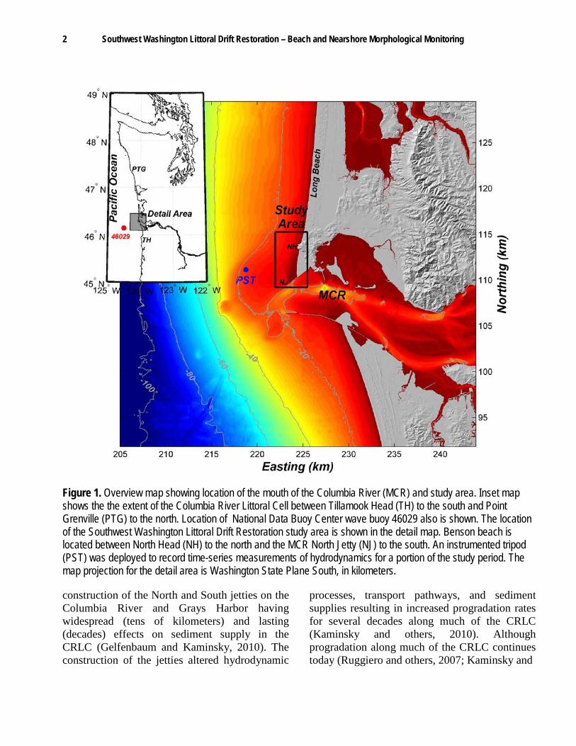
The CRLC extends from Tillamook Head, Oregon, to the south to Point Grenville, Washington, to the north (fig. 1). The beaches within the CRLC are sandy with broad surf zones and multiple sandbars (Ruggiero and others, 2005). Significant morphological change occurs over seasonal cycles because of variability in water levels and wave forcing throughout the year (Ruggiero and others, 2009). Over the past century, shoreline change within the CRLC has been dominated by human interventions, with the
2 Southwest Washington Littoral Drift Restoration – Beach and Nearshore Morphological Monitoring
Figure 1. Overview map showing location of the mouth of the Columbia River (MCR) and study area. Inset map shows the the extent of the Columbia River Littoral Cell between Tillamook Head (TH) to the south and Point Grenville (PTG) to the north. Location of National Data Buoy Center wave buoy 46029 also is shown. The location of the Southwest Washington Littoral Drift Restoration study area is shown in the detail map. Benson beach is located between North Head (NH) to the north and the MCR North Jetty (NJ) to the south. An instrumented tripod (PST) was deployed to record time-series measurements of hydrodynamics for a portion of the study period. The map projection for the detail area is Washington State Plane South, in kilometers.
construction of the North and South jetties on the Columbia River and Grays Harbor having widespread (tens of kilometers) and lasting (decades) effects on sediment supply in the CRLC (Gelfenbaum and Kaminsky, 2010). The construction of the jetties altered hydrodynamic
processes, transport pathways, and sediment supplies resulting in increased progradation rates for several decades along much of the CRLC (Kaminsky and others, 2010). Although progradation along much of the CRLC continues today (Ruggiero and others, 2007; Kaminsky and

Methods 3
others, 2010), erosion has been observed at several locations within the CRLC. One such area with pronounced erosion in recent years is Benson Beach.
Benson Beach is a 3-km stretch of coastline located between the mouth of the Columbia River (MCR) North Jetty to the south and North Head to the north (fig. 1) at the southern end of the Long Beach peninsula. Benson Beach formed as a direct result of the construction of the North Jetty between 1913 and 1917 (Kaminsky and others, 2010). The rapid progradation (as much as 54 m/yr) of Benson Beach continued until the 1950s when the shoreline began to erode (8.2 m/yr between the 1950s and 1999). Benson Beach is a popular recreation location that fronts the Cape Disappointment State Park and campground. The beach and shoreface also act as a barrier protecting the North Jetty infrastructure from damaging waves. Although a variety of factors contribute to the recent erosion at Benson Beach, the dominant factor is likely the loss of a sufficient local sediment supply from the depleted ebb-tidal delta. Another contributing factor appears to be regular maintenance dredging of the navigation channel at the MCR and offshore disposal, which has reduced the littoral sediment budget (Kaminsky and others, 2010). Based on trend analysis of historical shoreline change along Benson Beach between 1951 and 2001, Kaminsky and others (2003) predicted future erosion rates between 3 and 15 m/yr over the next 30 years. The direct placement of sand on the subaerial beach at Benson Beach thus should increase overall sediment supply and reduce local erosion.
Nourishment and Survey Design The Southwest Washington Littoral Drift
Restoration (SWLDR) project was carried out to assess the long-term viability of placing dredged material from the MCR directly on the beach to supplement the littoral sediment budget. Between July 13 and September 20, 2010, approximately 280,000 m3 of dredged sand from the MCR was
placed on Benson Beach (U.S. Army Corps of Engineers, written commun., 2010). Sediment dredged from the navigational channel in the MCR was hydraulically placed within a nominally rectangular permit area that extended roughly 275 m cross-shore and 400 m alongshore. The dredged material was placed from just seaward of the primary dune to the lower intertidal (approximately -1 m NAVD88), with the intention of forming a distinct morphological feature (salient) with a target thickness of about 2.5 m.
A morphological monitoring program was designed to document the condition of the beach immediately prior to the placement of nourishment material, and to characterize morphological change during and after the placement of nourishment material. Repeat surveys of nearshore bathymetry and beach topography were performed between July 11, 2010 and November 23, 2011. Bathymetric and topographic measurements were collected primarily along a series of cross-shore transects that extended from roughly the -10 m contour to just-landward of the primary dune crest (fig. 2). The survey design incorporated cross-shore transects that have been occupied annually since 1998 as part of the Southwest Washington coastal monitoring program (Ruggiero and others, 2005; Gelfenbaum and Kaminsky, 2010). Additional transects were inserted between the preexisting lines to achieve 50-m line spacing throughout the study area. The additional survey lines were approximately half as long as the long-term monitoring program lines, extending to roughly the -7 m depth contour. Surveys were conducted during spring tides with nearshore bathymetric measurements made during high tide, and topographic measurements collected during low tide to maximize coverage of the study area.
Equipment and Data Collection
Nearshore Bathymetry Nearshore bathymetry was measured
using single-beam sonar systems and GPS

4 Southwest Washington Littoral Drift Restoration – Beach and Nearshore Morphological Monitoring
Figure 2. Map showing survey design for the Southwest Washington Littoral Drift Restoration (SWLDR) morphological monitoring program (red lines) and base station used for geodetic control (magenta triangle). Locations of measurements made as part of the broader SWLDR monitoring program also are included— tracer deployment sites (black circles), tracer recovery sites (cyan squares), the North Head Argus camera (blue star), and locations of beach pods deployed to measure surf-zone hydrodynamics (blue circles). The location of the nourishment permit area is shown in yellow.
receivers mounted on personal watercraft (PWC) (fig. 3A). The number of PWCs used for each survey ranged from 2 to 4, depending on available personnel and equipment. The sonar systems consisted of an Odom© Echotrac CV-100 single-beam echosounder and 200 kHz transducer (9° beam angle). Raw acoustic backscatter returns were digitized by the echosounder with a vertical resolution of 1.25 cm. Depths from the echosounder were computed assuming a sound velocity of 1,500 m/s. The horizontal and vertical position of the survey vessels was determined at 20-Hz using Trimble® R7 GPS receivers with Zephyr 2 GPS antennas operating in real-time kinematic (RTK) mode. Differential corrections were transmitted to the PWC receivers at 1-Hz from a base station consisting of a Trimble® R7 receiver, a Trimble® L1/L2 GPS antenna, and a 35-watt Pacific Crest© radio transmitter. The base station was placed on a pre-existing benchmark (table 1; fig. 2) established as part of the Washington Coastal Geodetic Control Network (Daniels and others, 1999; Daniels and others, 2001). Output from the RTK-GPS and sonar systems were combined in real time on the PWC by a computer running HYPACK® hydrographic survey software. Electronic components of the survey systems were housed in water-tight cases and attached to the stern of the survey vessels. Navigation information was displayed on a video monitor, allowing PWC operators to navigate along survey lines at speeds of 2–3 m/s.
Bathymetric data were downloaded from the survey computers and post-processed using a custom Graphical User Interface (GUI) programmed with the computer program MATLAB®. Digitized depths were compared to the raw acoustic backscatter signal to ensure accuracy of depths produced by the echosounder, and the GUI was used to digitize the bottom by hand where the echosounder signal processing failed. This was common in the surf zone, where turbulence and bubbles in the water column added noise to the acoustic signal. After the raw depths were adjusted, a running mean with a

Methods 5
Table 1. Information about the benchmark used to establish geodetic control for Southwest Washington Littoral Drift Restoration surveys.
Property Value
Designation 944 0574 C Tidal National Geodetic Survey PID SD0297 Reference Frame NAD83 (1991) Latitude† N 46° 16’ 35.91561” Longitude† W 124° 03’ 59.09172” Northing (Washington State Plane South)† 111061.382 m Easting (Washington State Plane South)† 225226.997 m Ellipsoid Height -19.651 m Orthometric Height (NAVD88)* 4.678 m
*Orthometric height was determined by differential leveling and adjusted by the National Geodetic Survey (NGS) in 1991.
†Horizontal position of the benchmark was surveyed to first order standards as reported in Daniels and others (2001), but was not updated in the NGS database.
Figure 3. Photographs of the equipment used during field data collection showing A, personal watercraft (PWC) equipped with single-beam sonar system, RTK-GPS, and navigation computer, B, surveyor equipped with RTK-GPS mounted on a backpack, C, an all-terrain vehicle equipped with RTK-GPS, and D, PWC collecting data in the surf zone.

6 Southwest Washington Littoral Drift Restoration – Beach and Nearshore Morphological Monitoring
window length of 5–20 points (1–6 m distance) was used to remove high-frequency vertical fluctuations, such as those caused by pitch and roll of the survey vessels. Processed bathymetric data (x,y,z) from each survey line were exported as tab-delimited text files for further analysis.
Beach Topography The topographic beach measurements
were collected with RTK-GPS equipment identical to that described above in section, “Nearshore Bathymetry.” Cross-shore profiles were surveyed on foot with RTK-GPS equipment mounted on backpacks (fig. 3B). Small hand-held controllers were used to store the data and display real-time navigational information. Prior to data collection, vertical distances between the GPS antenna and the ground were measured by tape measure for each topographic surveyor. Cross-shore profiles were surveyed on the same series of transects as the nearshore bathymetry by walking with the rover unit from the landward edge of the primary dune, over the dune crest, to wading depth. Data for three-dimensional surface maps of the subaerial beach were collected using RTK-GPS equipment mounted on an all-terrain vehicle (ATV) (fig. 3C). The ATV was driven at different elevations on the beach until sufficient data were collected to determine both the alongshore and cross-shore morphologic variability. A typical survey at Benson Beach required roughly 45 km of ATV surveying. The combination of data from cross-shore profiles and surface maps resulted in an average point density of 0.046 ±0.007 elevation measurements/m2 on the beach over the entire monitoring program.
Horizontal and Vertical Accuracy Bathymetric and topographic elevation
measurements are subject to several sources of error, both random and systematic. The primary instruments for both bathymetric and topographic measurements in this study were the Trimble® R7 survey-grade GPS receivers. The random error associated with these units is approximately ±3 cm + 2 ppm in the horizontal and approximately
±5 cm + 2 ppm in the vertical while operating in RTK surveying mode, where ppm is relative to the distance (baseline) to the GPS base station (Trimble Navigation Limited, 2003). Baselines during this survey were less than 3 km, resulting in estimated horizontal uncertainty of ±4 cm, and vertical uncertainty of ±6 cm. In addition to random errors, GPS positions are subject to additional errors associated with multi-path, satellite obstructions, poor satellite geometry, and atmospheric conditions that can produce a systematic vertical GPS drift of as much as 10 cm (Sallenger and others, 2003). Ruggiero and others (2005) empirically estimated this systematic GPS drift to be approximately 4 cm.
Repeatability tests were performed to estimate the random uncertainty of elevation measurements collected by both bathymetric and topographic surveying platforms. Differences between topographic elevation measurements from walking surveys performed by different surveyors were quantified by comparing crossing points. Typically, root mean square (RMS) differences in elevation measurements for points collected within 1 m of each other by different surveyors and by the ATV were less than 5 cm (fig. 4). For bathymetric measurements, analysis of repeat bathymetric survey lines suggests RMS errors of vertical elevations measurements were typically less than 5 cm (fig. 5) for points within 1 m of each other. Mean offsets between survey vessels or surveyors on the beach were typically minimal (1–3 cm). Occasionally, static vertical adjustments were applied to data from a particular platform if mean offsets were greater than 3 cm.
Repeatability tests and comparison of nearshore bathymetry to overlapping topographic data suggests sub-decimeter vertical accuracy within a single bathymetric survey. However, variability in seawater temperature and salinity (not measured) affect the speed of sound in water, and thus the calculated depth for sonar measurements. Model output obtained from the calibrated 3-dimensional model, Virtual Columbia River (Baptista and others, 2005), were

Methods 7
Figure 4. Results of an example repeatability test between topographic data collected by two different survey operators. A, Map showing location of data collected by each surveyor and crossing points (shown in green), B, scatter plot showing a comparison of elevations obtained by Surveyor 1 versus Surveyor 2. Statistical measures defined in Willmott (1982) describing the difference between the two are provided, and C, histogram of residual elevations between Surveyor 1 and Surveyor 2.

8 Southwest Washington Littoral Drift Restoration – Beach and Nearshore Morphological Monitoring
Figure 5. Results of an example repeatability test for bathymetric data collected by two different survey vessels. A, Plot of elevation versus cross-shore distance showing location of data collected by each survey vessel, B, scatter plot showing a comparison of elevations obtained by Vessel 1 versus Vessel 2 for data points collected within 1 m of each other, and C, histogram of residual elevations between Vessel 1 and Vessel 2. Statistical measures describing the difference between the two are provided.

Methods 9
used to estimate how fluctuations in seawater properties would affect depth measurements on the days for which bathymetric surveys were conducted. These data suggest that variations in the speed of sound of seawater can alter depth estimates by approximately 1 percent of water depth in the study area. We therefore estimate the total uncertainty of bathymetric measurements, σtotal, by combining the random and depth-dependent components of uncertainty as follows (after Byrnes and others, 2002):
2 2
1
n
totaln
a n b d
(1)
where a is independent random components of uncertainty, b is the depth dependent uncertainty factor (0.01), and d is water depth. Assuming that the random uncertainty for the bathymetric measurements are equivalent to those of the topographic measurements estimated by Ruggiero and others (2005) (8 cm), equation 1 yields a total vertical uncertainty between 8 cm for topographic data and 26 cm for the deepest portions of the survey area.
Data Analysis Continuous surfaces were constructed
from processed bathymetric and topographic point data using linear interpolation with a grid resolution of 5 m. All available data were used to generate the gridded surfaces. The gridded surfaces were manually edited to ensure that the linear interpolation did not interpolate across areas not covered by field measurements. Changes in elevation and associated volume change within the study area were computed by calculating the difference between surveys at each grid point. Only elevation changes greater than the combined uncertainty for the two surveys being compared were included in the volume change analysis. The position of the shoreline was defined for each survey as the +2 m NAVD88 contour, which is roughly equivalent to mean high water at this location.
The movement of nearshore sandbars was quantified using several metrics of bar and trough morphology that were extracted in the following manner. Bathymetric and topographic data from each cross-shore profile were merged and interpolated at 5-m resolution. A Dean-type equilibrium cross-shore profile (Dean, 1991) was fit through the data, and the positions of bar crests and troughs were extracted by computing a local maximum and minimum on the elevation difference between survey data and the equilibrium profile. The bar positions were visually inspected and adjusted manually if the automatic algorithm failed to compute acceptable bar positions. Bar height was defined as the elevation difference between the bar crest and nearest landward trough. The bar depth was the elevation of the bar crest, and the distance from shore was calculated as the distance from the bar crest to the 3-m contour. Only subtidal bars, or those with bar depths deeper than approximately -0.5 m NAVD88, were quantified during this study.
Spatial and Temporal Survey Coverage Between July 11, 2010, and November
23, 2011, a total of 21 surveys were performed on Benson Beach. Eight surveys included both nearshore bathymetry and beach topography, and only topographic measurements were collected during the remaining 13 surveys (table 2). Survey S01 was conducted 20 days prior to commencement of sand-placement operations in order to characterize the morphology of the beach and nearshore prior to the nourishment. Surveys S02–S05 were conducted while sand was being placed on the beach, and survey S06 was conducted immediately following the completion of the beach nourishment. Surveys S07–S21 were conducted at roughly monthly intervals after completion of the nourishment.
Individual survey coverage varied depending on environmental conditions (tides and waves), equipment, and personnel availability. During favorable survey conditions (small waves and large tide range during daylight hours),

10 Southwest Washington Littoral Drift Restoration – Beach and Nearshore Morphological Monitoring
Table 2. List of survey identifications, survey dates, profiles collected and total linear distance covered for each survey.
Survey ID Survey Date
(YYYY/MM/DD) Topographic Data Bathymetric Data
Profiles Collected
Total Distance (km)
Profiles Collected Total Distance (km)
Nour
insh
men
t
S01 2010/07/11 61 84.5 66 110.0
S02 2010/08/10 67 75.0 67 75.2
S03 2010/08/25 53 33.7 0 0.0
S04 2010/09/01 60 46.1 0 0.0
S05 2010/09/10 62 81.8 0 0.0
S06 2010/09/22 62 94.2 78 92.0
Win
ter
S07 2010/10/06 60 39.7 63 48.2
S08 2010/10/27 60 36.6 0 0.0
S09 2010/11/04 60 55.7 0 0.0
S10 2010/12/05 60 75.3 66 68.8
S11 2011/01/20 60 69.9 0 0.0
S12 2011/02/17 60 70.6 0 0.0
S13 2011/03/23 60 67.2 0 0.0
S14 2011/04/19 61 81.3 0 0.0
Sum
mer
S15 2011/05/18 62 96.5 3 3.5
S16 2011/06/17 63 90.9 0 0.0
S17 2011/07/18 61 96.6 57 73.4
S18 2011/08/15 62 102.7 54 64.0
Win
ter S19 2011/09/29 62 94.4 0 0.0
S20 2011/10/27 61 68.4 0 0.0
S21 2011/11/04 60 69.7 0 0.0
overlap between bathymetric and topographic measurements resulted in complete cross-shore coverage of the beach and nearshore regions (fig. 6). Unfavorable survey conditions resulted in a gap between topographic and bathymetric measurements. For example, nearshore bathymetric coverage was limited in survey S07 (October 6, 2010) because of large waves (table 3) that prevented data collection in the shallow nearshore. Surveys conducted while sand was
being placed on the beach were limited in the area adjacent to the active sand placement operations due to unsafe working conditions. The bathymetric portion of survey S15 (May 19, 2011) was not completed because of damage sustained by one of the sonar systems. Maps showing data coverage for each survey are provided in appendix A.

Methods 11
Table 3. Environmental conditions during each bathymetric survey including wave height, wave period, wave direction, and wind speed measured at National Data Buoy Center buoy 46029. [Water temperature and salinity are from the calibrated operational model, Virtual Columbia River. For each parameter, the daily mean and standard deviation (in parenthesis) are provided] Survey Survey Date
(YYYY/MM/DD) Wave Height
(m) Wave Period
(s) Wave
Direction (°) Wind Speed
(m/s) Water Temp.
(°C) Salinity
(psu)
S01 2010/07/11 1.5 (0.07) 7.4 (0.30) 301.6 (4.28) 3.8 (1.81) 13.3 (1.5) 29.8 (5.2) S02 2010/08/10 1.1 (0.08) 11.5 (5.25) 249.5 (43.94) 3.6 (0.81) 13.6 (1.4) 29.0 (4.3) S06 2010/09/22 0.9 (0.08) 11.3 (0.54) 281.0 (5.43) 2.0 (1.01) 14.3 (0.6) 27.7 (3.6) S07 2010/10/06 2.0 (0.13) 11.1 (0.34) 285.4 (2.61) 4.0 (0.76) 14.0 (0.4) 28.1 (3.7) S10 2010/12/05 1.7 (0.13) 10.5 (0.44) 227.6 (24.56) 8.4 (0.96) 10.8 (0.8) 28.7 (4.1) S15 2011/05/18 1.5 (0.25) 8.5 (2.3) 283.5 (38.4) 7.7 (1.29) N/A N/A S17 2011/07/18 1.2 (0.15) 9.1 (0.53) 301.5 (16.3) 3.3 (2.47) 16.9 (0.8) 23.2 (6.1) S18 2011/08/15 0.9 (0.07) 13.5 (0.59) 272.3 (15.3) 1.2 (1.7) 15.1 (1.4) 28.6 (5.0)
Figure 6. Maps showing examples of A, bathymetric and topographic data coverage during an individual survey, B, processed data showing elevation of individual data points (color scale), and C, gridded elevation surface produced using linear interpolation with 5-m grid resolution.
12 Southwest Washington Littoral Drift Restoration – Beach and Nearshore Morphological Monitoring
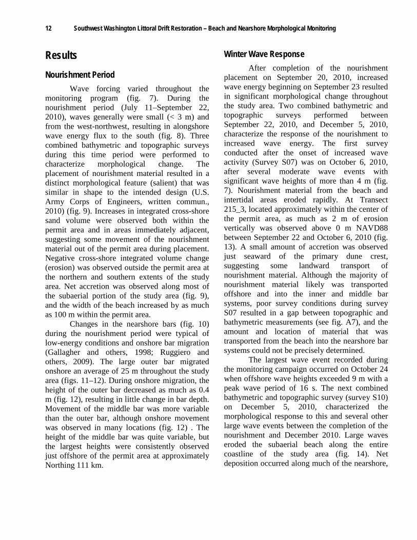
Results Nourishment Period
Wave forcing varied throughout the monitoring program (fig. 7). During the nourishment period (July 11–September 22, 2010), waves generally were small (< 3 m) and from the west-northwest, resulting in alongshore wave energy flux to the south (fig. 8). Three combined bathymetric and topographic surveys during this time period were performed to characterize morphological change. The placement of nourishment material resulted in a distinct morphological feature (salient) that was similar in shape to the intended design (U.S. Army Corps of Engineers, written commun., 2010) (fig. 9). Increases in integrated cross-shore sand volume were observed both within the permit area and in areas immediately adjacent, suggesting some movement of the nourishment material out of the permit area during placement. Negative cross-shore integrated volume change (erosion) was observed outside the permit area at the northern and southern extents of the study area. Net accretion was observed along most of the subaerial portion of the study area (fig. 9), and the width of the beach increased by as much as 100 m within the permit area.
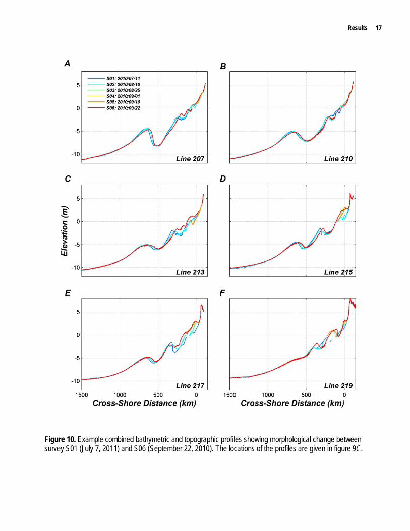
Changes in the nearshore bars (fig. 10) during the nourishment period were typical of low-energy conditions and onshore bar migration (Gallagher and others, 1998; Ruggiero and others, 2009). The large outer bar migrated onshore an average of 25 m throughout the study area (figs. 11–12). During onshore migration, the height of the outer bar decreased as much as 0.4 m (fig. 12), resulting in little change in bar depth. Movement of the middle bar was more variable than the outer bar, although onshore movement was observed in many locations (fig. 12) . The height of the middle bar was quite variable, but the largest heights were consistently observed just offshore of the permit area at approximately Northing 111 km.
Winter Wave Response After completion of the nourishment
placement on September 20, 2010, increased wave energy beginning on September 23 resulted in significant morphological change throughout the study area. Two combined bathymetric and topographic surveys performed between September 22, 2010, and December 5, 2010, characterize the response of the nourishment to increased wave energy. The first survey conducted after the onset of increased wave activity (Survey S07) was on October 6, 2010, after several moderate wave events with significant wave heights of more than 4 m (fig. 7). Nourishment material from the beach and intertidal areas eroded rapidly. At Transect 215_3, located approximately within the center of the permit area, as much as 2 m of erosion vertically was observed above 0 m NAVD88 between September 22 and October 6, 2010 (fig. 13). A small amount of accretion was observed just seaward of the primary dune crest, suggesting some landward transport of nourishment material. Although the majority of nourishment material likely was transported offshore and into the inner and middle bar systems, poor survey conditions during survey S07 resulted in a gap between topographic and bathymetric measurements (see fig. A7), and the amount and location of material that was transported from the beach into the nearshore bar systems could not be precisely determined.
The largest wave event recorded during the monitoring campaign occurred on October 24 when offshore wave heights exceeded 9 m with a peak wave period of 16 s. The next combined bathymetric and topographic survey (survey S10) on December 5, 2010, characterized the morphological response to this and several other large wave events between the completion of the nourishment and December 2010. Large waves eroded the subaerial beach along the entire coastline of the study area (fig. 14). Net deposition occurred along much of the nearshore,

Results 13
Figure 7. Time series of A, significant wave height, B, peak wave period, C, mean wave direction (the direction waves are coming from), and D, nourishment volume placed on the beach during the Southwest Washington Littoral Drift Restoration monitoring program. Wave parameters were obtained from National Data Buoy Center wave buoy 46029. See figure 1 for the location of buoy 46029 relative to the study site. Surveys 1-21 are indicated by red (combined bathymetry and topography) or blue (topography only) vertical lines through panels A-D.

14 Southwest Washington Littoral Drift Restoration – Beach and Nearshore Morphological Monitoring
Figure 8. Time series of A, weekly averaged cross-shore wave energy flux, and B, cumulative alongshore wave energy flux calculated from data at National Data Buoy Center buoy 46029 throughout the Southwest Washington Littoral Drift Restoration morphological monitoring program. In B, positive values denote cumulative northward wave energy flux and negative values denote cumulative energy flux to the south. See figure 1 for the location of buoy 46029 relative to the study site.

Results 15
suggesting that sediment from the beach was transported cross-shore and into the nearshore bars. Although large amounts of sediment were mobilized during this time period (gross volume change was 2 million m3), net volume change was minimal (-30,000 m3)(fig. 14D), suggesting that most of the morphological change was dominated by cross-shore sediment exchange.
Substantial changes to the position and morphology of the nearshore bars occurred during this time period of larger waves (figs. 15–17). Between surveys S06 and S07 (moderate wave conditions), the middle bar migrated offshore (see line 210, fig. 15). The outer bar continued to migrate onshore, and in the central portion of the study area, the height of the outer bar increased, resulting in a shoaling of the outer bar (fig. 17). Large waves (peak Hs > 9 m) that occurred between surveys S07 and S10 caused significant reorganization of the nearshore bars. In the central and southern parts of the study area (south of Northing 112 km), a three bar system developed where previously only two subtidal bars had been present (fig. 16). Shoaling of the outer bar trough (fig. 15) and offshore migration of the outer bar crest (fig. 17) suggest offshore movement of sediment during this time period.
A third combined bathymetric and topographic survey was attempted on May 18, 2011 (fig. 7), to characterize the bars at the end of the winter time period but was aborted due to damage to one of the sonar systems after collection of only three cross-shore profiles (table 2).
Summer Recovery Two combined bathymetric and
topographic surveys, S17 (July 18, 2011) and S18 (August 15, 2011), were conducted to characterize the morphological response of the beach and nearshore following a decrease in wave energy that occurred on April 2011. As a
result of a large gap in time between survey S17 and the previous successful combined bathymetry and topography survey (survey S10, December 5, 2010), the observed morphological change integrated over a wide range of forcing conditions. Following survey S10, wave energy remained high throughout the winter with frequent wave events with significant wave heights exceeding 4 m at the National Data Buoy Center (NDBC) wave buoy (fig. 7). Wave energy decreased in April and remained relatively low throughout the remainder of the summer (April 19, 2010–September 15, 2011). The subaerial beach experienced net erosion in the central portion of the study area and net accretion at the northern and southern extents (fig. 18). Accretion of the subaerial beach was particularly evident at the southern end of the study area where the +2-m contour was displaced seaward as much as 50 m away from the MCR North Jetty (fig. 18D). Cross-shore integrated volume change was negative along much of the study area, indicating net loss of sediment from the study area.
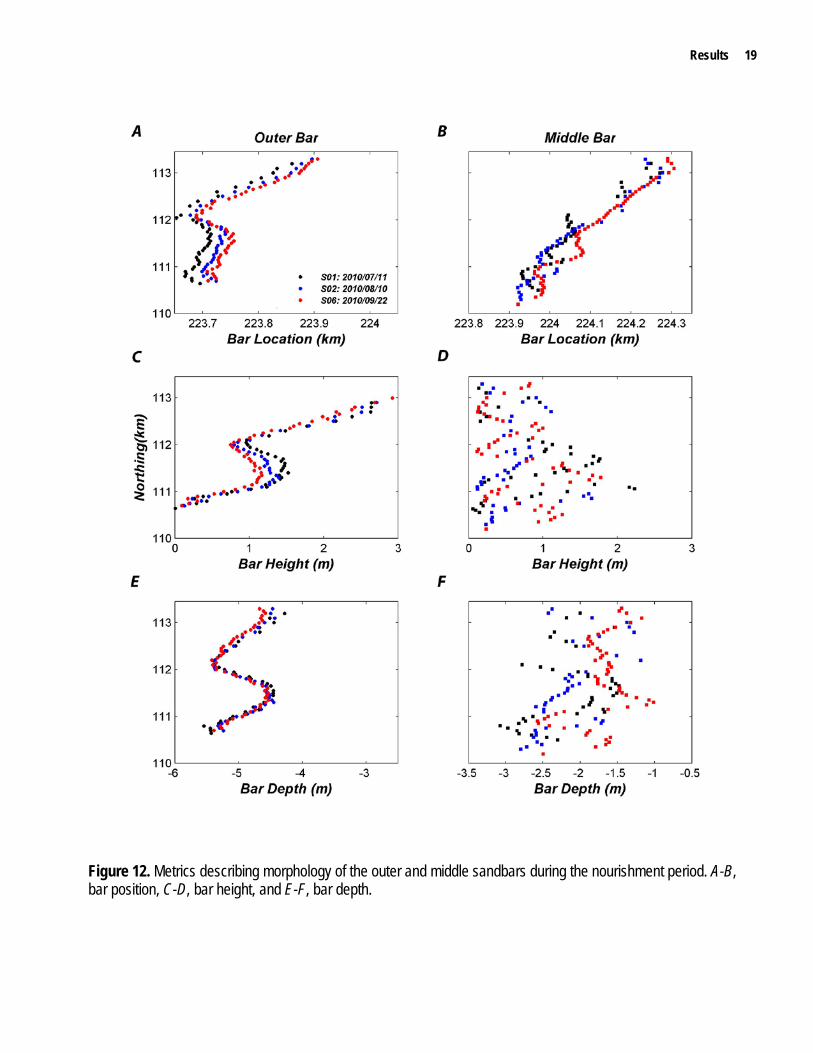
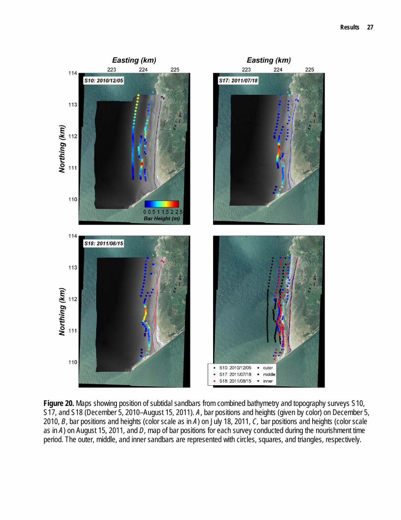
The pattern of erosion and deposition observed in figure 18C was largely related to changes in the nearshore bars (figs. 19–21). The nearshore, which had been characterized as a 2–3 subtidal bar system, changed primarily to a single bar system between December 5, 2010, and July 18, 2011. The outer bar that had been present throughout the SWLDR monitoring program disappeared completely (fig. 20). The outer bar during survey S17 was located more than 200 m landward of the outer bar position observed during survey S10, and outer bar depths changed from roughly -5.5 m to approximately -4 m (fig. 21).
Little morphologic change was observed between the two combined bathymetric and topographic surveys conducted during summer 2011 (surveys S17 and S18), and the changes primarily were associated with onshore bar migration (fig. 19).

16 Southwest Washington Littoral Drift Restoration – Beach and Nearshore Morphological Monitoring
Figure 9. Results of combined bathymetry and topography surveys conducted dring the nourishment period. A, gridded elevation surface for the pre-nourishment survey (S01) conducted on July 11, 2010, B, gridded elevation surface for the post-nourishment survey (S06) conducted on September 22, 2010, C, elevation difference between the two surveys, and D, cross-shore averaged volume change (gray bars) and shoreline change (red line) computed at 200-m intervals along the study area. The nourishment permit area polygon is included in A–C. The location of combined bathymetric and topographic profiles shown in figure 10 are given in C.
Results 17
Figure 10. Example combined bathymetric and topographic profiles showing morphological change between survey S01 (July 7, 2011) and S06 (September 22, 2010). The locations of the profiles are given in figure 9C.

18 Southwest Washington Littoral Drift Restoration – Beach and Nearshore Morphological Monitoring
Figure 11. Maps showing position of subtidal sandbars during the nourishment period. A, bar positions and heights (given by color) on July 11, 2010, B, bar positions and heights (color scale as in A) on August 10, 2010, C, bar positions and heights (color scale as in A) on September 22, 2010, and D, map of bar positions for each survey conducted during the nourishment time period. The outer, middle, and inner sandbars are represented with circles, squares, and triangles, respectively.
Results 19
Figure 12. Metrics describing morphology of the outer and middle sandbars during the nourishment period. A-B, bar position, C-D, bar height, and E-F, bar depth.

20 Southwest Washington Littoral Drift Restoration – Beach and Nearshore Morphological Monitoring
Figure 13. Results of morphological monitoring showing initial response of the nourishment to moderate wave conditions. A, Time-series of significant wave height measured at National Data Buoy Center buoy 46029. Surveys S06 and S07 (gray vertical lines) were conducted before and after the onset higher wave energy. B, Erosion and deposition measured between surveys S07 and S06. C, An example profile taken from the approximate center of the beach nourishment showing erosion of the subaerial beach, offshore bar migration of the middle bar, and onshore bar migration of the outer bar. The location of the profile is shown in B.

Results 21
Figure 14. Results of combined bathymetry and topography surveys conducted between surveys S06 and S10 (September 22–December 5, 2010). A, gridded elevation surface for survey S06 conducted on September 22, 2010, B, gridded elevation surface for the survey S10 conducted on December 5, 2010, C, elevation difference between the two surveys, and D, cross-shore averaged volume change (gray bars) and shoreline change (red line) computed at 200-m intervals along the study area. The nourishment permit area polygon is included in A-C. The location of combined bathymetric and topographic profiles shown in figure 15 are given in C.

22 Southwest Washington Littoral Drift Restoration – Beach and Nearshore Morphological Monitoring
Figure 15. Example combined bathymetric and topographic profiles showing morphological change between surveys S06 and S10 (September 22–December 5, 2010). The locations of profiles are given in figure 14C.

Results 23
Figure 16. Maps showing position of subtidal sandbars from combined bathymetry and topography surveys S06, S07, S10 (September 22–December 5, 2010). A, bar positions and heights (given by color) on September 22, 2010, B, bar positions and heights (color scale as in A) on October 6, 2010, C, bar positions and heights (color scale as in A) on December 5, 2010, and D, map of bar positions for each survey performed during the nourishment time period. The outer, middle, and inner sandbars are represented with circles, squares, and triangles, respectively.

24 Southwest Washington Littoral Drift Restoration – Beach and Nearshore Morphological Monitoring
Figure 17. Metrics describing morphology of the outer and middle sandbars from combined bathymetry and topography surveys S06, S07, and S10 (September 22–December 5, 2010). A–B, bar position, C–D, bar height, and E–F, bar depth.

Results 25
Figure 18. Results of combined bathymetry and topography surveys conducted between surveys S10 and S18 (December 5, 2010–August 15, 2011). A, gridded elevation surface for survey S10 conducted on December 5, 2010, B, gridded elevation surface for the survey S18 conducted on August 15, 2011, C, elevation difference between the two surveys, and D, cross-shore averaged volume change (gray bars) and shoreline change (red line) computed at 200-m intervals along the study area. The nourishment permit area polygon is included in A-C. The location of combined bathymetric and topographic profiles shown in figure 19 are given in C.
26 Southwest Washington Littoral Drift Restoration – Beach and Nearshore Morphological Monitoring
Figure 19. Example combined bathymetric and topographic profiles showing morphological change between surveys S10 and S18 (December 5, 2010–August 15, 2011). The locations of profiles are given in figure 18C.
Results 27
Figure 20. Maps showing position of subtidal sandbars from combined bathymetry and topography surveys S10, S17, and S18 (December 5, 2010–August 15, 2011). A, bar positions and heights (given by color) on December 5, 2010, B, bar positions and heights (color scale as in A) on July 18, 2011, C, bar positions and heights (color scale as in A) on August 15, 2011, and D, map of bar positions for each survey conducted during the nourishment time period. The outer, middle, and inner sandbars are represented with circles, squares, and triangles, respectively.

28 Southwest Washington Littoral Drift Restoration – Beach and Nearshore Morphological Monitoring
Figure 21. Metrics describing morphology of the outer and middle sandbars from combined bathymetry and topography surveys S10, S17, and S18 (December 5, 2010–August 15, 2011). A–B, bar position, C–D, bar height, and E–F, bar depth.

Discussion 29
Discussion Detectable changes in the elevation of the
beach and upper shoreface were observed throughout the study area during the SWLDR morphological monitoring program (figs. 22–23). In the discussion that follows, we present an initial interpretation of the observed morphological change to document the placement and dispersal of SWLDR nourishment and to characterize the physical environment in which it was placed. However, further insight into the processes responsible for the dispersal of the nourishment may be obtained by combining the morphological monitoring data with a hydrodynamic and sediment transport model constructed for the MCR (Elias and others, 2011), and with additional data from Argus video monitoring, nearshore and surf-zone hydrodynamic measurements, and a physical tracer experiment that were collected as part of the broader SWLDR monitoring program (fig. 2).
Cumulative Shoreline and Volume Change The study area was divided into three
regions in the alongshore and three regions in the cross-shore in order to track sediment movement within the study area (fig. 24). The alongshore regions were defined relative to the nourishment permit area: south, within the permit area, and north of the permit area. The cross-shore regions were defined based on the morphology of the initial survey: beach (above -1 m NAVD88), inner nearshore (including inner and middle sandbars), and outer nearshore (including the outer bar and seaward). Changes in sand volumes within each polygon were computed for all combined bathymetry and topography surveys relative to the pre-nourishment survey (S01). For the topography-only surveys, volume change was computed for three beach regions only.
Low Wave Energy during Nourishment Placement Net volume change within the defined
polygons occurred throughout the SWLDR
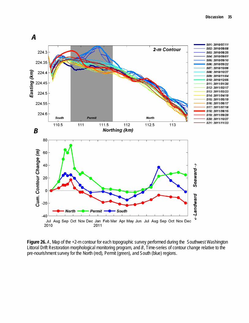
monitoring period (fig. 25). Between the initial survey and the completion of the nourishment, the three beach regions gained a total of 444,000 m3 of sediment with 61 percent (272,000 m3) of the observed sediment accumulation occurring within the nourishment permit area (table 4). Net accretion within the three beach polygons exceeded the total amount of nourishment material placed on the beach (280,000 m3). During placement of the nourishment, two natural processes likely contributed to the observed volume change. First, relatively low wave energy caused the inner and middle bars to migrate onshore (fig. 12), transporting material from the inner nearshore onto the subaerial beach. In addition to this cross-shore exchange, waves and tides forced some alongshore sediment transport during placement. Throughout the nourishment placement, offshore wave forcing was consistently from the northwest (fig. 8) and likely resulted in alongshore transport of both nourishment and native sediment to the south towards the MCR North Jetty. The total volume change within the inner nearshore and beach polygons was 274,000 m3, suggesting that most (more than 97 percent) of the nourishment remained within the beach and inner nearshore during placement. Net deposition of sediment on the subaerial beach resulted in seaward displacement of the 2-m contour (fig. 26). During the nourishment, the 2-m contour prograded an average of 25, 72, and 17 m for the South, Permit, and North regions, respectively.
Rapid Erosion of the Nourishment from the Beach Higher wave energy during the winter
resulted in rapid decreases in sediment volume within the three beach polygons (fig. 25A), and landward displacement of the 2-m contour (fig. 26). The moderate wave conditions that occurred between surveys S06 and S07 (2-week time period) resulted in a total of 211,000 m3 of erosion from the three beach polygons and landward displacement of the 2-m contour within the permit area by 36 m. The inner nearshore regions experienced increases in volume (total of

30 Southwest Washington Littoral Drift Restoration – Beach and Nearshore Morphological Monitoring
Figure 22. Maps of interpolated bathymetric and topographic data from surveys: A, S01: July 11, 2012, B, S06: September 22, 2010, C, S10: December 5, 2010, and D, S18: August 15, 2011.
A B
C D

Discussion 31
Figure 23. Maps showing elevation difference computed between interpolated surfaces for A, the nourishment period (S06-S01); B, early winter (S10-S06) , C, summer recovery (S18-S10), and D, cumulative change (S18-S01).
A B
C D

32 Southwest Washington Littoral Drift Restoration – Beach and Nearshore Morphological Monitoring
Figure 24. Map showing location of polygons used for volume change analysis. The study area was divided into three regions in the cross-shore (outer nearshore, inner nearshore, and beach) and three regions in the alongshore (north, permit, and south).

Discussion 33
Figure 25. Time series of cumulative volume change (103 m3) for the A, beach, B, inner nearshore, C, outer nearshore regions, and D, net change throughout the study area. For each cross-shore region, cumulative volume change for the North (red), Permit (green), and South (blue) polygons are shown. Total change for each cross-shore region is given in yellow. The volume of nourishment sand placed on the beach is provided in A.

34 Southwest Washington Littoral Drift Restoration – Beach and Nearshore Morphological Monitoring
Table 4. Cumulative volume change (103 m3) within the beach, inner nearshore and outer nearshore regions. [Differences were computed between the pre-nourishment survey (S01) and each subsequent survey. Net volume change is reported for combined topography and bathymetry surveys only. See figure 24 for the locations of the regions] Beach Inner Nearshore Outer Nearshore Net Survey Survey Date
(YYYY/MM/DD) North Permit South North Permit South North Permit South
Nour
insh
men
t S01 2010/07/11 - - - - - - - - - - S02 2010/08/10 10.9 85.0 45.7 -91.1 -11.8 -1.8 23.5 11.8 -15.4 56.8 S03 2010/08/25 21.6 154.2 44.2 - - - - - - - S04 2010/09/01 30.8 130.3 28.4 - - - - - - - S05 2010/09/10 51.4 213.5 75.2 - - - - - - S06 2010/09/22 87.9 272.2 83.9 -145.0 -6.0 -19.4 32.3 21.7 -56.9 270.5
Win
ter
S07 2010/10/06 6.3 187.4 39.0 -35.2* 52.2* 8.2* 21.4 7.1 -106.0 180.3* S08 2010/10/27 -57.2 91.5 13.6 - - - - - - - S09 2010/11/04 -57.1 98.0 2.2 - - - - - - - S10 2010/12/05 -106.6 98.8 -30.4 201.9 145.7 53.9 -46.2 -19.6 -115.4 182.2 S11 2011/01/20 -160.5 -0.3 -10.5 - - - - - - - S12 2011/02/17 -125.1 10.7 -33.0 - - - - - - - S13 2011/03/23 -197.4 -0.9 -27.1 - - - - - - - S14 2011/04/19 -220.6 5.8 -57.5 - - - - - - -
Sum
mer
S15 2011/05/18 -169.3 13.2 -29.0 - - - - - - - S16 2011/06/17 -157.1 35.2 -17.9 - - - - - - - S17 2011/07/18 -127.6 84.8 -5.9 232.4 205.0 -55.2 -352.6 -299.9 -138.0 -457.0 S18 2011/08/15 -58.7 143.9 37.0 222.9 189.6 -73.7 -329.1 -280.5 -166.9 -315.4
Win
ter S19 2011/09/29 -113.9 141.5 15.9 - - - - - - -
S20 2011/10/27 -103.6 169.3 2.5 - - - - - - - S21 2011/11/23 -131.5 108.6 -6.2 - - - - - - -
*Limited coverage of the Inner Nearshore Regions
196,000 m3) and the middle bar migrated seaward (fig. 17), suggesting that most of the nourishment material was transported into the nearshore bars. The salient created during the placement of the nourishment did not respond coherently to the increased wave energy. Rather, the nourishment material likely spread out as it was transported offshore into the inner and middle bars (fig. 13) and was no longer recognizable as a distinct feature on October 6, 2010, 16 days after the nourishment placement was complete.
After the initial wave response, the volume of sediment within the three beach polygons continued to decrease throughout the early winter, with a total loss of approximately 482,000 m3 of sand from the three beach polygons between surveys S06 and S10
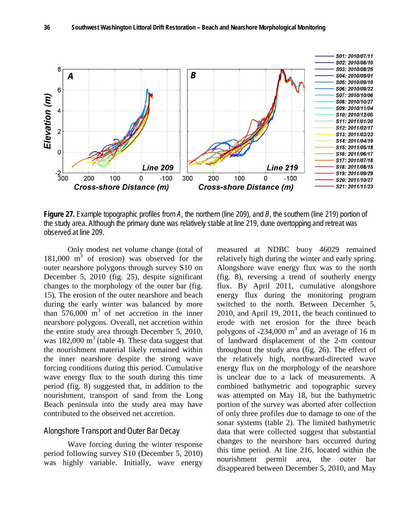
(September 22, 2010–December 5, 2011). Despite its rapid erosion, the nourishment appeared to have a buffering effect on beach erosion in the permit area and adjacent area to the south. The 2-m contour within the permit area remained near the postion of the pre-nourishment survey throughout the winter (fig. 26). In contrast, north of the permit area, net beach erosion and landward displacement of the 2-m contour was observed relative to pre-nourishment. Dune overtopping and retreat in the late winter and spring was limited to the northern part of the study area (fig. 27), although the lack of dune erosion in the permit and south regions may alternatively have been due to higher initial dune crests.
Discussion 35
Figure 26. A, Map of the +2-m contour for each topographic survey performed during the Southwest Washington Littoral Drift Restoration morphological monitoring program, and B, Time-series of contour change relative to the pre-nourishment survey for the North (red), Permit (green), and South (blue) regions.
36 Southwest Washington Littoral Drift Restoration – Beach and Nearshore Morphological Monitoring
Figure 27. Example topographic profiles from A, the northern (line 209), and B, the southern (line 219) portion of the study area. Although the primary dune was relatively stable at line 219, dune overtopping and retreat was observed at line 209.
Only modest net volume change (total of 181,000 m3 of erosion) was observed for the outer nearshore polygons through survey S10 on December 5, 2010 (fig. 25), despite significant changes to the morphology of the outer bar (fig. 15). The erosion of the outer nearshore and beach during the early winter was balanced by more than 576,000 m3 of net accretion in the inner nearshore polygons. Overall, net accretion within the entire study area through December 5, 2010, was 182,000 m3 (table 4). These data suggest that the nourishment material likely remained within the inner nearshore despite the strong wave forcing conditions during this period. Cumulative wave energy flux to the south during this time period (fig. 8) suggested that, in addition to the nourishment, transport of sand from the Long Beach peninsula into the study area may have contributed to the observed net accretion.
Alongshore Transport and Outer Bar Decay Wave forcing during the winter response
period following survey S10 (December 5, 2010) was highly variable. Initially, wave energy
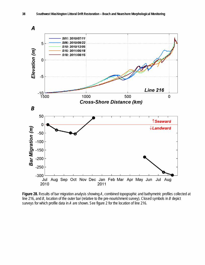
measured at NDBC buoy 46029 remained relatively high during the winter and early spring. Alongshore wave energy flux was to the north (fig. 8), reversing a trend of southerly energy flux. By April 2011, cumulative alongshore energy flux during the monitoring program switched to the north. Between December 5, 2010, and April 19, 2011, the beach continued to erode with net erosion for the three beach polygons of -234,000 m3 and an average of 16 m of landward displacement of the 2-m contour throughout the study area (fig. 26). The effect of the relatively high, northward-directed wave energy flux on the morphology of the nearshore is unclear due to a lack of measurements. A combined bathymetric and topographic survey was attempted on May 18, but the bathymetric portion of the survey was aborted after collection of only three profiles due to damage to one of the sonar systems (table 2). The limited bathymetric data that were collected suggest that substantial changes to the nearshore bars occurred during this time period. At line 216, located within the nourishment permit area, the outer bar disappeared between December 5, 2010, and May

Discussion 37
18, 2011. The new outer bar was located more than 250 m landward (fig. 28) of the position of the outer bar recorded on December 5, 2010.
The change in configuration of the nearshore bar system observed at line 216 was representative of morphological changes observed throughout the nearshore during the final two combined bathymetric and topographic surveys conducted in the summer 2011 (fig. 18). Throughout the study area, the outer bar had disappeared (fig. 20). The loss of the outer bar was accompanied by large net volume change within the study area, particularly in the three outer polygons, where net volume change was -609,000 m3 (fig. 25). Strong northward, alongshore wave-energy flux and net erosion in the study area suggests that wave-driven currents and alongshore sediment transport played an important role in the decay of the outer bar. These observations are consistent with recent modeling and field observations that have identified wave-driven alongshore current as a primary mechanism responsible for bar migration and decay (Walstra and others, 2012). Aagaard and others (2010) observed that bar decay at a site along the Danish North Sea coast was associated with local net sediment loss and collected direct measurements of boundary-layer hydrodynamics and sediment transport associated with bar decay. Their results suggested that the net loss of sediment was associated with alongshore-directed transport by processes not associated with breaking waves. The loss of the outer bar at Benson Beach likely is part of an interannual trend of offshore bar migration and decay that has been observed along many sandy coastlines (Ruessink and Kroon, 1994; Plant and others, 1999). Additional analysis of previous datasets would be needed to understand how the seasonal observations of bar migration and decay reported herein are related to longer term (interannual) time-scales at Benson Beach.
Long-Term Effect of Nourishment on Shoreline Change
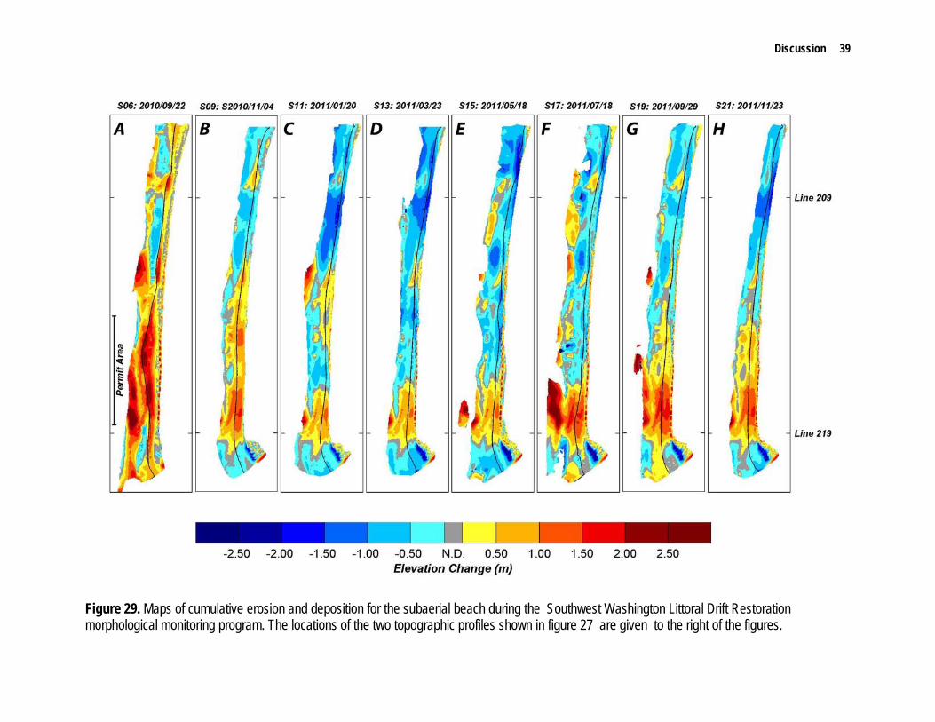
Wave-energy flux decreased significantly during the summer recovery period (April–August 2011) (fig. 8). The lower energy conditions resulted in net deposition within the three beach polygons (fig. 25) and seaward displacement of the 2-m contour (fig. 26). The recovery on the beach was most pronounced in the south and permit areas where seaward displacement of the 2-m contour was 52 and 25 m, respectively, at the end of the summer recovery (survey S18). Over the entire SWLDR monitoring program, net erosion was observed to the north of the permit area, although net deposition occurred within the permit area and the adjacent area to the south (fig. 29). This pattern of erosion and deposition may be due to natural gradients in alongshore transport causing net movement of sediment from north to south. Alternatively, nourishment material may have remained in the system and contributed to the enhanced recovery of the beach during the beach recovery the following summer. The long-term persistence of small nourishments in regions with large seasonal variability in wave forcing has been documented elsewhere (Yates and others, 2009). A small beach nourishment (160,000 m3) placed on Torrey Pines beach in southern California rapidly eroded in response to a storm with significant wave heights of 3 m (Seymour and others, 2005). During the storm, the nourishment material was transported offshore as an enhanced sandbar. Subsequent monitoring revealed that the nourishment material remained within the littoral system and was later transported onshore and contributed to increased rates of shoreline accretion relative to unnourished portions of the coast (Yates and others, 2009). The data collected at Benson Beach are consistent with this scenario and suggest a possible long-term (annual) benefit of the nourishment for reducing erosion rates locally.
38 Southwest Washington Littoral Drift Restoration – Beach and Nearshore Morphological Monitoring
Figure 28. Results of bar migration analysis showing A, combined topographic and bathymetric profiles collected at line 216, and B, location of the outer bar (relative to the pre-nourishment survey). Closed symbols in B depict surveys for which profile data in A are shown. See figure 2 for the location of line 216.
Discussion 39
Figure 29. Maps of cumulative erosion and deposition for the subaerial beach during the Southwest Washington Littoral Drift Restoration morphological monitoring program. The locations of the two topographic profiles shown in figure 27 are given to the right of the figures.

40 Southwest Washington Littoral Drift Restoration – Beach and Nearshore Morphological Monitoring
Summary A morphological monitoring program
documented the placement and initial dispersal of a nourishment (280,000 m3) placed on a high-energy, modally-dissipative coastline at Benson Beach in southwestern Washington State. The results of the monitoring program suggest that placement of the nourishment created a distinct morphological feature that was similar in shape and morphology to the intended design. During placement, southerly alongshore transport resulted in movement of nourishment material to the south towards the MCR North Jetty. Moderate wave conditions (Hs about 4 m) that occurred between the completion of the nourishment on September 20, 2010, and October 6, 2010, resulted in cross-shore sediment transport with most of the nourishment material transported into the nearshore bars, although some accretion also was observed landward at the toe of the primary dune. During the subsequent period of increased wave energy, the nourishment acted as a buffer to the more severe erosion, including dune overtopping and retreat, that was observed at the northern end of the study area. One year after placement of the nourishment, onshore transport and beach recovery was most pronounced within the permit area and to the south toward the MCR North Jetty. This suggests that there is some long-term benefit of the nourishment for reducing erosion rates locally, although the enhanced recovery also could be due to natural gradients in alongshore transport causing net movement of the sediment from north to south.
Measurements made during the morphological monitoring program documented the seasonal movement and decay of nearshore sand bars over the course of the year. Late summer, low-energy conditions resulted in onshore bar migration early in the monitoring program. Moderate wave conditions in the autumn resulted in offshore movement of the middle bar and continued onshore migration of the outer bar. High-energy wave conditions early
in the winter resulted in strong cross-shore transport and creation of a 3-bar system along portions of the coast. More southerly wave events occurred later in the winter and early spring and coincided with the complete loss of the outer bar and net loss of sediment from the study area. These data suggest that bar decay may be an important mechanism for exporting sediment from Benson Beach north to the Long Beach Peninsula.
Acknowledgments Funding for this work was provided by
the U.S. Army Corps of Engineers Portland District, the U.S. Geological Survey Coastal and Marine Geology Program, and from the Northwest Association of Networked Ocean Observing Systems (NANOOS). We thank Hans Rod Moritz from the Portland District Army Corps of Engineers for overall project coordination. This report would not have been possible without the hard work of many researchers, technicians, and graduate students who spent long hours on the beach and on the water collecting the field data. We acknowledge in particular the efforts of Andrew Schwartz from the Washington State Department of Ecology who kept the togpographic data collection machine functioning and Heather Baron from Oregon State University who, in addition to participating in most of the bathymetric surveys, coordinated the field work logistics among the participating groups. The rest of the field team (a.k.a the Nearshore All-Stars) included Erica Harris, Jeremy Mull, Jeff Wood, Katy Serafin, Diana DiLeonardo, Justin Brodersen, and Sarah Kassem from Oregon State University, Diana McCandless, Andrew Ryan, Gabrielle Stillwater, Grant Dunster, Brandt Lyse, Debra Molsberry, and Margo Mansfield from the Washington State Department of Ecology, and Josh Logan from the U.S. Geological Survey. An earlier version of this report was improved by reviews by David Thomson and Dan Hoover.

References Cited 41
References Cited Aagaard, T., Kroon, A., Greenwood, B., and
Hughes, M.G., 2010, Observations of offshore bar decay—Sediment budgets and the role of lower shoreface processes: Continental Shelf Research, v. 30, p. 1,497–1,510.
Baptista, A.M., Zhang, Y., Chawla, A., Zulauf, M., Seaton, C., Myers, E.P., III, Kindle, J., Wilkin, M., Burla, M., and Turner, P.J., 2005, A cross-scale model for 3D baroclinic circulation in estuary-plume-shelf systems—II. Application to the Columbia River: Continental Shelf Research, v. 25, p. 935–972.
Barnard, P.L., Erikson, L.H, and Hansen, J.E., 2009, Monitoring and modeling shoreline response due to shoreface nourishment on a high-energy coast: Journal of Coastal Research, v. SI56, p. 29–33.
Browder, A.E., and Dean, R.G., 2000, Monitoring and comparison to predictive models of the Perdido Key beach nourishment project, Florida, USA: Coastal Engineering, v. 39, p. 173–191.
Byrnes, M.R., Baker, J.L., and Li, Feng (2002), Quantifying potential measurement errors associated with bathymetric change analysis: ERDC/CHL CHETN-IV-50, U.S. Army Engineer Research and Development Center, Vicksburg, Miss. 17 p.
Daniels, R.C., Ruggiero, P., and Weber, L.E., 1999, Washington coastal geodetic control network— Report and station index: Washington Department of Ecology, Coastal Monitoring & Analysis Program, Publication #99-103, 268 p.
Daniels, R.C., McCandless, D.C., Huxford, R.H., Kingsley, E.D., and Ruggiero, P., 2001, Update to the Washington Coastal Geodetic Control Network: Washington State Department of Ecology, Coastal Monitoring and Analysis Program, Publication no. 01-06-013, 22 p.
Dean, R.G., 1991, Equilibrium beach profiles—Characteristics and applications: Journal of Coastal Research, v. 7, p. 53–84.
Dean, R.G., 2002, Beach Nourishment—Theory and Practice: River Edge, N.J., World Scientific, 399 p.
Elias, E., Gelfenbaum, G., van Ormondt, M., and Moritz, H.R., 2011, Predicting sediment transport patterns at the mouth of the Columbia River, in Rosati, J.D., Wang, P., and Roberts, T.M., eds., Proceedings of the Coastal Sediments, Hackensack, N.J., World Scientific Publishing, p. 588–601.
Gelfenbaum, G., and Kaminsky, G.M., 2010, Large-scale coastal change in the Columbia River littoral cell—An overview: Marine Geology, v. 273, p. 1–10.
Gallagher, E.L., Elgar, S., and Guza, R.T., 1998, Observations of sand bar evolution on a natural beach: Journal of Geophysical Research, v. 103, p. 3,203–3,215.
Grunnet, N.M., Walstra, D.J.R., and Ruessink, B.G., 2004, Process-based modeling of a shoreface nourishment: Coastal Engineering, v. 51, p. 581–607.
Grunnet, N.M., and Ruessink, B.G., 2005, Morphodynamic response of nearshore bars to a shoreface nourishment: Coastal Engineering, v. 52, p. 119–137.
Hamm, L., Capocianco, M., Dette, H.H., Lechuga, A., Spanhoff, R., Stive, M.J.F., 2002, A summary of European experience with shore nourishment: Coastal Engineering, v. 47, p. 237–264.
Kaminsky, G.M., Buijsman, M.C., McCandless, D., and Ruggiero, P., 2003, Erosion potential analysis of Benson Beach: Washington Department of Ecology, Coastal Monitoring and Analysis Program, Publication no. 05-06-101, 78 p.
Kaminsky, G.M., Ruggiero, P., Buijsman, M.C., McCandless, D., and Gelfenbaum, G., 2010, Historical evolution of the Columbia River littoral cell: Marine Geology, v. 273, p. 96–126.
Moerman, E., 2011, Long-term morphological modeling of the mouth of the Columbia River:, Delft University of Technology, Delft, The Netherlands, Masters thesis, 154 p.

42 Southwest Washington Littoral Drift Restoration – Beach and Nearshore Morphological Monitoring
Plant, N.G., Holman, R.A., Freilich, M.H., and Birkemeier, W.A., 1999, A simple model for interannual sandbar behavior: Journal of Geophysical Research, v. 104, p. 15,755–15,776.
Ruessink, B.G., and Kroon, A., 1994, The behavior of a multiple bar system in the nearshore zone of Terschelling, the Netherlands—1,965-1,993: Marine Geology, v. 121, p. 187–197.
Ruggiero, P., Kaminsky, G.M., Gelfenbaum, G., and Voigt, B., 2005, Seasonal to interannual morphodynamics along a high-energy dissipative littoral cell: Journal of Coastal Research, v. 21, p. 553–578.
Ruggiero, P., Eshleman, J.L., Kingsley, E., Thompson, D.M., Voigt, B., Kaminsky, G.M., and Gelfenbaum, G., 2007, Beach morphology monitoring in the Columbia River littoral cell—1997-2005: U.S. Geological Survey Data Series 260, 88 p.
Ruggiero, P., Walstra, D.J.R., Gelfenbaum, G., and van Ormondt, M., 2009, Seasonal-scale morphological evolution—Field observations and numerical modeling: Coastal Engineering, v. 56, p. 1,153–1,172.
Trimble Navigation Limited, 2003, Trimble R7/R8 GPS receiver user guide, 216 p.
Sallenger, A.H., Krabill, W.B., Swift, R.N., Brock, J., List, J., Hansen, M., Holman, R.A., Manizade, S., Sontag, J., Meredith, A., Morgan, K., Yunkel, J.K., Frederick, E.B., and Stockdon, H., 2003. Evaluation of airborne topographic lidar for quantifying beach changes: Journal of Coastal Research, v. 19, p. 125-133.
Seymour, R., Guza, R.T., O’Reilly, W., and Elgar, S., 2005, Rapid erosion of a small southern California beach fill: Coastal Engineering, v. 52, p. 151–158.
Walstra, D.J.R., Reniers, A.J.H.M., Ranasinghe, R., Roelvink, J.A., and Ruessink, B.G., 2012, On bar growth and decay during interannual net offshore migration: Coastal Engineering, v. 60, p. 190–200.
Willmott, C.J., 1982, Some comments on the evaluation of model performance: Bulletin of
the American Meteorological Society, v. 63, p. 1,309–1,313.
Yates, M.L., Guza, R.T., O’Reilly, W.C., and Seymour, R.J., 2009, Seasonal persistence of a small southern California beach fill: Coastal Engineering, v. 59, p. 559–564.

Appendix A. Data Coverage and Personnel 43
Appendix A. Data Coverage and Personnel Maps of data coverage for each survey performed during the Southwest Washington Littoral
Drift Restoration monitoring program are shown in figures A1-A21. Table A1 provides the USGS Field Activity and webpage link to metadata for each survey. Table A2 provides a list of personnel and affiliations for all participants in the field monitoring program.
Table A1. List of survey numbers, survey dates, USGS field activity identification numbers, and webpage links where metadata about each survey is archived.
Survey Date Field Activity ID
Metadata Webpage
S01 2010/07/11 W-1-10-WO http://walrus.wr.usgs.gov/infobank/w/w110wo/html/w-1-10-wo.meta.html S02 2010/08/08 W-2-10-WO http://walrus.wr.usgs.gov/infobank/w/w210wo/html/w-2-10-wo.meta.html S03 2010/08/25 W-S1-10-WA http://walrus.wr.usgs.gov/infobank/w/ws110wa/html/w-s1-10-wa.meta.html S04 2010/09/01 W-S2-10-WA http://walrus.wr.usgs.gov/infobank/w/ws210wa/html/w-s2-10-wa.meta.html S05 2010/09/10 W-S3-10-WA http://walrus.wr.usgs.gov/infobank/w/ws310wa/html/w-s3-10-wa.meta.html S06 2010/09/22 W-4-10-WO http://walrus.wr.usgs.gov/infobank/w/w410wo/html/w-4-10-wo.meta.html S07 2010/10/06 W-6-10-WO http://walrus.wr.usgs.gov/infobank/w/w610wo/html/w-6-10-wo.meta.html S08 2010/10/27 W-S4-10-WA http://walrus.wr.usgs.gov/infobank/w/ws410wa/html/w-s4-10-wa.meta.html S09 2010/11/04 W-S5-10-WA http://walrus.wr.usgs.gov/infobank/w/ws510wa/html/w-s5-10-wa.meta.html S10 2010/12/05 W-5-10-WO http://walrus.wr.usgs.gov/infobank/w/w510wo/html/w-5-10-wo.meta.html S11 2011/01/20 W-S1-11-WA http://walrus.wr.usgs.gov/infobank/w/ws111wa/html/w-s1-11-wa.meta.html S12 2011/02/17 W-S2-11-WA http://walrus.wr.usgs.gov/infobank/w/ws211wa/html/w-s2-11-wa.meta.html S13 2011/03/23 W-S3-11-WA http://walrus.wr.usgs.gov/infobank/w/ws311wa/html/w-s3-11-wa.meta.html S14 2011/04/19 W-S4-11-WA http://walrus.wr.usgs.gov/infobank/w/ws411wa/html/w-s4-11-wa.meta.html S15 2011/05/19 W-07-11-WO http://walrus.wr.usgs.gov/infobank/w/w0711wo/html/w-07-11-wo.meta.html S16 2011/06/17 W-S5-11-WA http://walrus.wr.usgs.gov/infobank/w/ws511wa/html/w-s5-11-wa.meta.html S17 2011/07/18 W-05-11-WO http://walrus.wr.usgs.gov/infobank/w/w0511wo/html/w-05-11-wo.meta.html S18 2011/08/15 W-06-11-WO http://walrus.wr.usgs.gov/infobank/w/w0611wo/html/w-06-11-wo.meta.html S19 2011/09/29 W-S6-11-WA http://walrus.wr.usgs.gov/infobank/w/ws611wa/html/w-s6-11-wa.meta.html S20 2011/10/27 W-S7-11-WA http://walrus.wr.usgs.gov/infobank/w/ws711wa/html/w-s7-11-wa.meta.html S21 2011/11/23 W-S8-11-WA http://walrus.wr.usgs.gov/infobank/w/ws811wa/html/w-s8-11-wa.meta.html

44 Southwest Washington Littoral Drift Restoration – Beach and Nearshore Morphological Monitoring
Table A2. List of personnel, affiliations, and the number of surveys each person participated in during the monitoring program.
Personnel Affiliation Number of Surveys
Guy Gelfenbaum U.S. Geological Survey 2
Andrew Stevens U.S. Geological Survey 6
Josh Logan U.S. Geological Survey 1
Peter Ruggiero Oregon State University 6
Heather Baron Oregon State University 6
Katy Serafin Oregon State University 3
Erica Harris Oregon State University 3
Justin Broderson Oregon State University 3
Jeremy Mull Oregon State University 3
Jeff Wood Oregon State University 4
Diana DiLeonardo Oregon State University 4
Sarah Kassem Oregon State University 1
George Kaminsky Washington State Department of Ecology 12
Diana McCandless Washington State Department of Ecology 14
Andrew Schwartz Washington State Department of Ecology 14
Andrew Ryan Washington State Department of Ecology 7
Gabrielle Stillwater Washington State Department of Ecology 6
Margot Mansfield Washington State Department of Ecology 1
Debra Molsberry Washington State Department of Ecology 1
Brandt Lyse Washington State Department of Ecology 1
Grant Dunster Washington State Department of Ecology 1

Appendix A. Data Coverage and Personnel 45
Figure A1. Maps of locations of nearshore bathymetric data (red) and topographic data (blue) collected during survey S01, July 11–12, 2010, showing the entire study area (at left) and the beach and shallow nearshore (at right).

46 Southwest Washington Littoral Drift Restoration – Beach and Nearshore Morphological Monitoring
Figure A2. Maps of locations of nearshore bathymetric data (red) and topographic data (blue) collected during survey S02, August 10, 2010, showing the entire study area (at left) and the beach and shallow nearshore (at right).

Appendix A. Data Coverage and Personnel 47
Figure A3. Maps of locations of topographic data (blue) collected during survey S03, August 25, 2010, showing the entire study area (at left) and the beach and shallow nearshore (at right).

48 Southwest Washington Littoral Drift Restoration – Beach and Nearshore Morphological Monitoring
Figure A4. Maps of locations topographic data (blue) collected during survey S04, September 1, 2010, showing the entire study area (at left) and the beach and shallow nearshore (at right).

Appendix A. Data Coverage and Personnel 49
Figure A5. Maps of locations topographic data (blue) collected during survey S05, September 10, 2010, showing the entire study area (at left) and the beach and shallow nearshore (at right).

50 Southwest Washington Littoral Drift Restoration – Beach and Nearshore Morphological Monitoring
Figure A6. Maps of locations of nearshore bathymetric data (red) and topographic data (blue) collected during survey S06, September 22, 2010, showing the entire study area (at left) and the beach and shallow nearshore (at right).

Appendix A. Data Coverage and Personnel 51
Figure A7. Maps of locations of nearshore bathymetric data (red) and topographic data (blue) collected during survey S07, October 6, 2010, showing the entire study area (at left) and the beach and shallow nearshore (at right).

52 Southwest Washington Littoral Drift Restoration – Beach and Nearshore Morphological Monitoring
Figure A8. Maps of locations of topographic data (blue) collected during survey S08, October 27, 2010, showing the entire study area (at left) and the beach and shallow nearshore (at right).

Appendix A. Data Coverage and Personnel 53
Figure A9. Maps of locations of topographic data (blue) collected during survey S09, November 4, 2010, showing the entire study area (at left) and the beach and shallow nearshore (at right).

54 Southwest Washington Littoral Drift Restoration – Beach and Nearshore Morphological Monitoring
Figure A10. Maps of locations of nearshore bathymetric data (red) and topographic data (blue) collected during survey S10, December 5, 2010, showing the entire study area (at left) and the beach and shallow nearshore (at right).

Appendix A. Data Coverage and Personnel 55
Figure A11. Maps of locations of topographic data (blue) collected during survey S11, January 20, 2011, showing the entire study area (at left) and the beach and shallow nearshore (at right).

56 Southwest Washington Littoral Drift Restoration – Beach and Nearshore Morphological Monitoring
Figure A12. Maps of locations of topographic data (blue) collected during survey S12, February 17, 2011, showing the entire study area (at left) and the beach and shallow nearshore (at right).
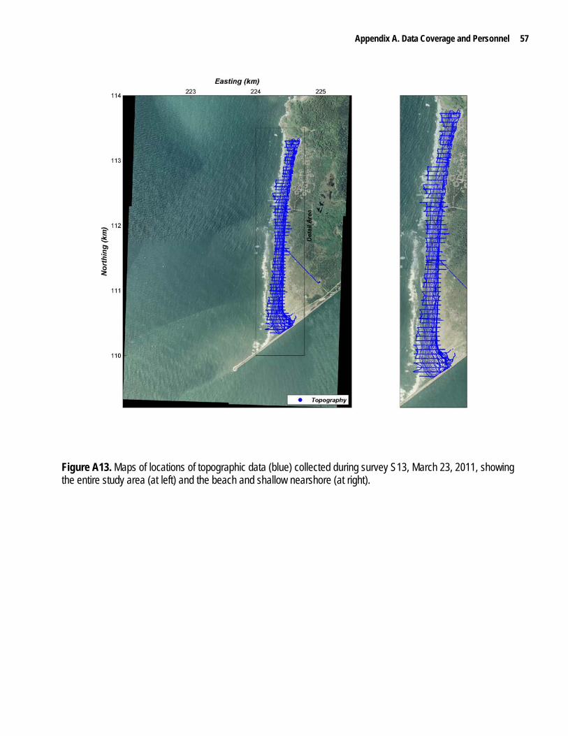
Appendix A. Data Coverage and Personnel 57
Figure A13. Maps of locations of topographic data (blue) collected during survey S13, March 23, 2011, showing the entire study area (at left) and the beach and shallow nearshore (at right).

58 Southwest Washington Littoral Drift Restoration – Beach and Nearshore Morphological Monitoring
Figure A14. Maps of locations of topographic data (blue) collected during survey S14, April 19, 2011, showing the entire study area (at left) and the beach and shallow nearshore (at

Appendix A. Data Coverage and Personnel 59
right).
Figure A15. Maps of locations of topographic data (blue) and bathymetric data (red) collected during survey S15, May 18, 2011, showing the entire study area (at left) and the beach and shallow nearshore (at right).

60 Southwest Washington Littoral Drift Restoration – Beach and Nearshore Morphological Monitoring
Figure A16. Maps of locations of topographic data (blue) collected during survey S16, June 17, 2011, showing the entire study area (at left) and the beach and shallow nearshore (at right).

Appendix A. Data Coverage and Personnel 61
Figure A17. Maps of locations of topographic data (blue) and bathymetric data (red) collected during survey S17, July 18, 2011, showing the entire study area (at left) and the beach and shallow nearshore (at right).
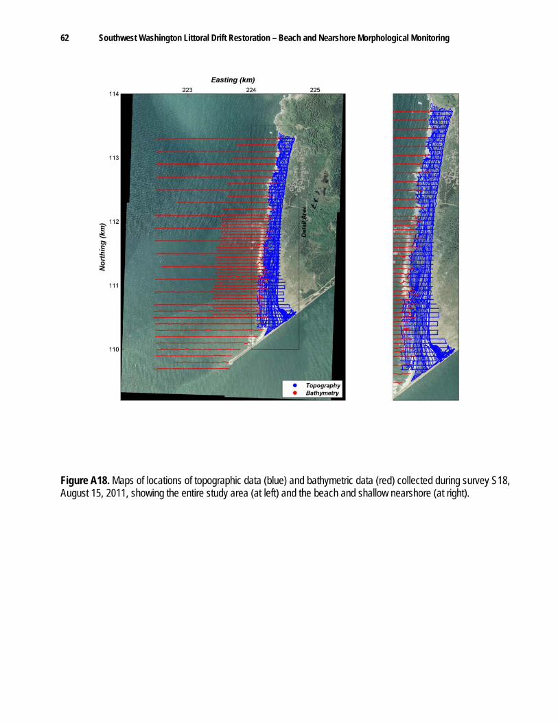
62 Southwest Washington Littoral Drift Restoration – Beach and Nearshore Morphological Monitoring
Figure A18. Maps of locations of topographic data (blue) and bathymetric data (red) collected during survey S18, August 15, 2011, showing the entire study area (at left) and the beach and shallow nearshore (at right).

Appendix A. Data Coverage and Personnel 63
Figure A19. Maps of locations of topographic data (blue) collected during survey S19, September 29, 2011, showing the entire study area (at left) and the beach and shallow nearshore (at right).
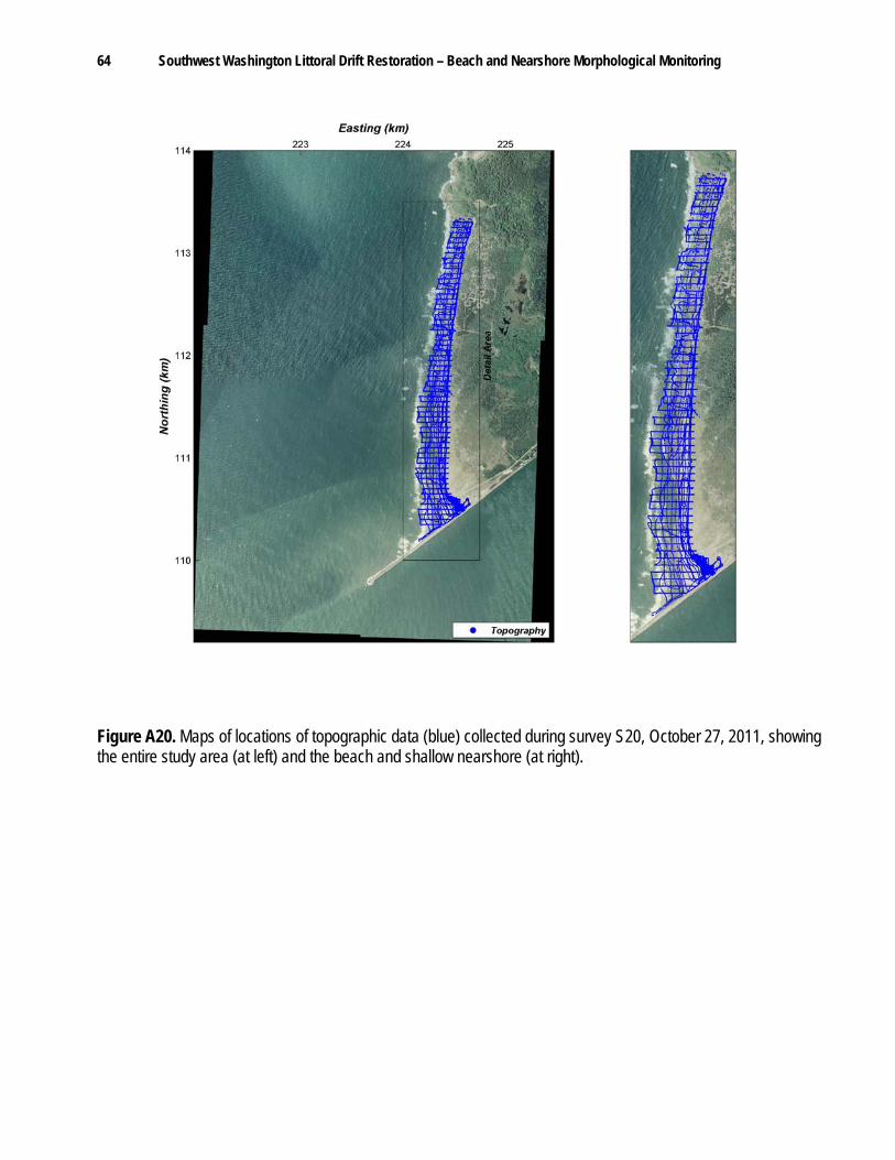
64 Southwest Washington Littoral Drift Restoration – Beach and Nearshore Morphological Monitoring
Figure A20. Maps of locations of topographic data (blue) collected during survey S20, October 27, 2011, showing the entire study area (at left) and the beach and shallow nearshore (at right).

Appendix A. Data Coverage and Personnel 65
Figure A21. Maps of locations of topographic data (blue) collected during survey S21, November 23, 2011, showing the entire study area (at left) and the beach and shallow nearshore (at right).

66 Southwest Washington Littoral Drift Restoration – Beach and Nearshore Morphological Monitoring
Appendix B. Data Tables Appendix B provides a description of the data provided from the Southwest Washington Littoral
Drift Restoration (SWLDR) morphological monitoring program. Elevations are provided in orthometric heights in the reference frame NAD83 (1991) and NAVD88. Horizontal positions are projected in the Washington State Plane South coordinate system, and all values (easting, northing, and elevation) are in meters. A zip file for each survey is provided (table B1) that includes elevation measurements in tab-delimited text files (*.txt) with easting, northing, elevation, and cross-shore transect identification number. Nearshore bathymetry and beach topography data are provided separately. Gridded data provided in ESRI ASCII GRID files (*.asc) and XYZ (*.xyz) formats, and FGDC compliant metadata in both text and .xml formats also are included in the zip files.
The ESRI ASCII GRID file consists of header information containing a set of six keywords, followed by cell values in row-major order. All gridded datasets provided for this study were interpolated with identical resolution and spatial extent, and therefore contain the same header information:
NCOLS 461 NROWS 981 XLLCORNER 222400.000 YLLCORNER 109650.000 CELLSIZE 5.000 NODATA_VALUE -999.999
The header is followed by a block of size (NROWS by NCOLS) of tab-delimited elevation data. Row 1 of the data is at the top of the grid, row 2 is just under row 1 and so on. The NODATA_VALUE is the value in the ASCII file to be assigned to those cells whose true value is unknown.
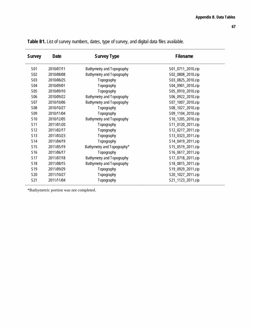
Appendix B. Data Tables
67
Table B1. List of survey numbers, dates, type of survey, and digital data files available.
Survey Date Survey Type Filename
S01 2010/07/11 Bathymetry and Topography S01_0711_2010.zip S02 2010/08/08 Bathymetry and Topography S02_0808_2010.zip S03 2010/08/25 Topography S03_0825_2010.zip S04 2010/09/01 Topography S04_0901_2010.zip S05 2010/09/10 Topography S05_0910_2010.zip S06 2010/09/22 Bathymetry and Topography S06_0922_2010.zip S07 2010/10/06 Bathymetry and Topography S07_1007_2010.zip S08 2010/10/27 Topography S08_1027_2010.zip S09 2010/11/04 Topography S09_1104_2010.zip S10 2010/12/05 Bathymetry and Topography S10_1205_2010.zip S11 2011/01/20 Topography S11_0120_2011.zip S12 2011/02/17 Topography S12_0217_2011.zip S13 2011/03/23 Topography S13_0323_2011.zip S14 2011/04/19 Topography S14_0419_2011.zip S15 2011/05/19 Bathymetry and Topography* S15_0519_2011.zip S16 2011/06/17 Topography S16_0617_2011.zip S17 2011/07/18 Bathymetry and Topography S17_0718_2011.zip S18 2011/08/15 Bathymetry and Topography S18_0815_2011.zip S19 2011/09/29 Topography S19_0929_2011.zip S20 2011/10/27 Topography S20_1027_2011.zip S21 2011/11/04 Topography S21_1123_2011.zip
*Bathymetric portion was not completed.