Thesis for the degree of Doctor of Philosophy

Source–Channel Coding in Networks

Niklas Wernersson

Communication TheorySchool of Electrical Engineering

KTH (Royal Institute of Technology)

Stockholm 2008

Wernersson, NiklasSource–Channel Coding in Networks

Copyright c©2008 Niklas Wernersson except whereotherwise stated. All rights reserved.

TRITA-EE 2008:028ISSN 1653-5146ISBN 978-91-7415-002-5

Communication TheorySchool of Eletrical EngineeringKTH (Royal Institute of Technology)SE-100 44 Stockholm, SwedenTelephone + 46 (0)8-790 7790

Abstract

The aim of source coding is to represent information as accurately as possible us-ing as few bits as possible and in order to do so redundancy from the source needsto be removed. The aim of channel coding is in some sense the contrary, namelyto introduce redundancy that can be exploited to protect the information when be-ing transmitted over a nonideal channel. Combining these two techniques leadsto the area of joint source–channel coding which in general makes it possible toachieve a better performance when designing a communication system than in thecase when source and channel codes are designed separately. In this thesis fourparticular areas in joint source–channel coding are studied: analog (i.e. continu-ous) bandwidth expansion, distributed source coding over noisy channels, multipledescription coding (MDC) and soft decoding.

A general analog bandwidth expansion code based on orthogonal polynomi-als is proposed and analyzed. The code has a performance comparable with otherexisting schemes. However, the code is more general in the sense that it is imple-mentable for a larger number of source distributions.

The problem of distributed source coding over noisy channels is studied. Twoschemes are proposed and analyzed for this problem which both work on a sampleby sample basis. The first code is based on scalar quantization optimized for acertain channel characteristics. The second code is nonlinear and analog.

Two new MDC schemes are proposed and investigated. The first is based onsorting a frame of samples and transmitting, as side-information/redundancy, anindex that describes the resulting permutation. In case that some of the transmit-ted descriptors are lost during transmission this side information (if received) canbe used to estimate the lost descriptors based on the received ones. The secondscheme uses permutation codes to produce different descriptions of a block ofsource data. These descriptions can be used jointly to estimate the original sourcedata. Finally, also the MDC method multiple description coding using pairwisecorrelating transforms as introduced by Wang et al. is studied. A modification ofthe quantization in this method is proposed which yields a performance gain.

A well known result in joint source–channel coding is that the performance ofa communication system can be improved by using soft decoding of the channeloutput at the cost of a higher decoding complexity. An alternative to this is toquantize the soft information and store the pre-calculated soft decision values in a

i

lookup table. In this thesis we propose new methods for quantizing soft channelinformation, to be used in conjunction with soft-decision source decoding. Theissue on how to best construct finite-bandwidth representations of soft informationis also studied.

Keywords: source coding, channel coding, joint source–channel coding, band-width expansion, distributed source coding, multiple description coding, soft de-coding.

ii

Acknowledgements

During my Ph.D. studies I have received a lot of help from various persons. Mostimportant by far has been the help from my supervisor Professor Mikael Skoglund.Mikael has been supportive since the day I started at KTH and he has always beenable to find time for our research discussions in his otherwise busy schedule. Hehas been actively interested in my work and always done his utmost in order toguide me. This has made him a great mentor and I would like to express mygratitude for all the help during these years.

I would further like to thank Professor Tor Ramstad for inviting me as a guestto NTNU. The visit at Tor’s research group was a great experience.

I devote special thanks to Tomas I Andersson, Johannes Karlsson and Pal An-ders Floor for work resulting in joint publications.

I would also like to thank all my current and past colleagues at KTH for all thevaluable support, both in a scientific way as well as a social way. In particular Iwould like to thank: Joakim for many interesting talks at KTH–hallen. Karl forteaching me about good manners as well as teaming up with me in F.E.M. Mats,Erik and Peter H for valuable research discussions. Svante for educating me aboutRansater. Magnus J and Per for XC–skiing inspiration. David and George forteaching me a thing or two about Stockholm. Xi and Peter v. W for inspiring meto smuggle a bike. Lei for always being so helpful. Patrick for many interestingmusic conversations. Tung for joining me in eating strange food in France. Henrikfor letting me make fun of his lunch habits. Nina and Niklas J for great parties.Tomas I and Marc for philosophical conversations. Bjorn L for all the never endinginformation at bonebanken. And finally, Karin, Marie and Annika for spreadinghappiness around the office with their positive way.

I further wish to thank the faculty opponent and the grading committee fortaking the time to be involved in the thesis defence.

Finally, I would like to thank my family back home (including grandmotherIngeborg and the Brattlofs; Greta and the Nordling families) since they have man-aged to support me during these years, although I have been at some distance away.The support was highly appreciated. Last but certainly not least, thank you Bar-bara for everything. Without you this journey would have been a lot tougher andfar less enjoyable.

iii

Contents

Abstract i

Acknowledgements iii

Contents v

I Introduction 1

Introduction 11 Source Coding . . . . . . . . . . . . . . . . . . . . . . . . . . . 2

1.1 Lossless Coding . . . . . . . . . . . . . . . . . . . . . . 31.2 Lossy Coding . . . . . . . . . . . . . . . . . . . . . . . . 3

2 Channel Coding . . . . . . . . . . . . . . . . . . . . . . . . . . . 93 The Source–Channel Separation Theorem . . . . . . . . . . . . . 104 Analog Source–Channel Coding . . . . . . . . . . . . . . . . . . 11

4.1 Analog Bandwidth Expansion . . . . . . . . . . . . . . . 124.2 Analog Bandwidth Compression . . . . . . . . . . . . . . 13

5 Distributed Source Coding . . . . . . . . . . . . . . . . . . . . . 145.1 Theoretical Results . . . . . . . . . . . . . . . . . . . . . 145.2 Practical Schemes . . . . . . . . . . . . . . . . . . . . . 18

6 Multiple Description Coding . . . . . . . . . . . . . . . . . . . . 196.1 Theoretical Results . . . . . . . . . . . . . . . . . . . . . 206.2 Practical Schemes . . . . . . . . . . . . . . . . . . . . . 21

7 Source Coding for Noisy Channels . . . . . . . . . . . . . . . . . 277.1 Scalar Source Coding for Noisy Channels . . . . . . . . . 287.2 Vector Source Coding for Noisy Channels . . . . . . . . . 297.3 Index Assignment . . . . . . . . . . . . . . . . . . . . . 31

8 Contributions of the Thesis . . . . . . . . . . . . . . . . . . . . . 31References . . . . . . . . . . . . . . . . . . . . . . . . . . . . . . . . . 36

v

II Included papers 45

A Polynomial Based Analog Source–Channel Codes A11 Introduction . . . . . . . . . . . . . . . . . . . . . . . . . . . . . A12 Problem Formulation . . . . . . . . . . . . . . . . . . . . . . . . A23 Orthogonal Polynomials . . . . . . . . . . . . . . . . . . . . . . A4

3.1 Definition . . . . . . . . . . . . . . . . . . . . . . . . . . A43.2 The recurrence formula and zeros . . . . . . . . . . . . . A43.3 Gram–Schmidt . . . . . . . . . . . . . . . . . . . . . . . A53.4 The Christoffel–Darboux identity . . . . . . . . . . . . . A6

4 Encoding and Decoding . . . . . . . . . . . . . . . . . . . . . . . A65 Analysis . . . . . . . . . . . . . . . . . . . . . . . . . . . . . . . A7

5.1 Distance . . . . . . . . . . . . . . . . . . . . . . . . . . . A75.2 Stretch . . . . . . . . . . . . . . . . . . . . . . . . . . . A85.3 Dimensions . . . . . . . . . . . . . . . . . . . . . . . . . A8

6 Simulations . . . . . . . . . . . . . . . . . . . . . . . . . . . . . A96.1 Choosing I . . . . . . . . . . . . . . . . . . . . . . . . . A96.2 Optimal companding and benchmark systems . . . . . . . A106.3 Results . . . . . . . . . . . . . . . . . . . . . . . . . . . A11

7 Conclusions . . . . . . . . . . . . . . . . . . . . . . . . . . . . . A13References . . . . . . . . . . . . . . . . . . . . . . . . . . . . . . . . . A13

B Distributed Quantization over Noisy Channels B11 Introduction . . . . . . . . . . . . . . . . . . . . . . . . . . . . . B12 Problem Formulation . . . . . . . . . . . . . . . . . . . . . . . . B2

2.1 Binary Symmetric Channel . . . . . . . . . . . . . . . . . B22.2 Gaussian Channel . . . . . . . . . . . . . . . . . . . . . . B3

3 Analysis . . . . . . . . . . . . . . . . . . . . . . . . . . . . . . . B43.1 Encoder for BSC . . . . . . . . . . . . . . . . . . . . . . B43.2 Encoder for Gaussian Channel . . . . . . . . . . . . . . . B53.3 Decoder . . . . . . . . . . . . . . . . . . . . . . . . . . . B63.4 Design algorithm . . . . . . . . . . . . . . . . . . . . . . B63.5 Optimal Performance Theoretically Attainable . . . . . . B7

4 Simulations . . . . . . . . . . . . . . . . . . . . . . . . . . . . . B74.1 Structure of the Codebook - BSC . . . . . . . . . . . . . B94.2 Structure of the Codebook - Gaussian Channel . . . . . . B94.3 Performance Evaluation . . . . . . . . . . . . . . . . . . B12

5 Conclusions . . . . . . . . . . . . . . . . . . . . . . . . . . . . . B14References . . . . . . . . . . . . . . . . . . . . . . . . . . . . . . . . . B16

vi

C Nonlinear Coding and Estimation for Correlated Data in WirelessSensor Networks C11 Introduction . . . . . . . . . . . . . . . . . . . . . . . . . . . . . C12 Problem Formulation . . . . . . . . . . . . . . . . . . . . . . . . C23 Discussion and Proposed Scheme . . . . . . . . . . . . . . . . . C3

3.1 σ2w > 0 and σ2

n → 0 . . . . . . . . . . . . . . . . . . . . C33.2 σ2

w = 0 and σ2n > 0 . . . . . . . . . . . . . . . . . . . . . C3

3.3 Objective . . . . . . . . . . . . . . . . . . . . . . . . . . C43.4 Analysis . . . . . . . . . . . . . . . . . . . . . . . . . . C53.5 Proposed Scheme . . . . . . . . . . . . . . . . . . . . . . C7

4 Performance Analysis . . . . . . . . . . . . . . . . . . . . . . . . C85 Simulations . . . . . . . . . . . . . . . . . . . . . . . . . . . . . C106 Conclusions . . . . . . . . . . . . . . . . . . . . . . . . . . . . . C12Appendix . . . . . . . . . . . . . . . . . . . . . . . . . . . . . . . . . C13References . . . . . . . . . . . . . . . . . . . . . . . . . . . . . . . . . C14

D Sorting–Based Multiple Description Quantization D11 Introduction . . . . . . . . . . . . . . . . . . . . . . . . . . . . . D12 Sorting-Based MDQ . . . . . . . . . . . . . . . . . . . . . . . . D13 Analysis . . . . . . . . . . . . . . . . . . . . . . . . . . . . . . . D44 Numerical Results . . . . . . . . . . . . . . . . . . . . . . . . . . D55 Conclusions . . . . . . . . . . . . . . . . . . . . . . . . . . . . . D8Appendix . . . . . . . . . . . . . . . . . . . . . . . . . . . . . . . . . D9References . . . . . . . . . . . . . . . . . . . . . . . . . . . . . . . . . D11Addendum to the Paper . . . . . . . . . . . . . . . . . . . . . . . . . . D12

E Multiple Description Coding using Rotated Permutation Codes E11 Introduction . . . . . . . . . . . . . . . . . . . . . . . . . . . . . E12 Preliminaries . . . . . . . . . . . . . . . . . . . . . . . . . . . . E23 Proposed MDC Scheme . . . . . . . . . . . . . . . . . . . . . . . E2

3.1 Calculating E[x|ij ] . . . . . . . . . . . . . . . . . . . . . E33.2 Calculating E[x|i1, · · · , iJ ] . . . . . . . . . . . . . . . . E43.3 The Effect of the Generating Random Matrices . . . . . . E6

4 Simulations . . . . . . . . . . . . . . . . . . . . . . . . . . . . . E64.1 Introducing More Design Parameters . . . . . . . . . . . E7

5 Conclusions . . . . . . . . . . . . . . . . . . . . . . . . . . . . . E8Appendix . . . . . . . . . . . . . . . . . . . . . . . . . . . . . . . . . E8Acknowledgments . . . . . . . . . . . . . . . . . . . . . . . . . . . . . E9References . . . . . . . . . . . . . . . . . . . . . . . . . . . . . . . . . E9

F Improved Quantization in Multiple Description Coding by Correlat-ing Transforms F11 Introduction . . . . . . . . . . . . . . . . . . . . . . . . . . . . . F12 Preliminaries . . . . . . . . . . . . . . . . . . . . . . . . . . . . F2

vii

3 Improving the Quantization . . . . . . . . . . . . . . . . . . . . . F44 Simulation Results . . . . . . . . . . . . . . . . . . . . . . . . . F65 Conclusions . . . . . . . . . . . . . . . . . . . . . . . . . . . . . F7References . . . . . . . . . . . . . . . . . . . . . . . . . . . . . . . . . F8

G On Source Decoding Based on Finite-Bandwidth Soft Information G11 Introduction . . . . . . . . . . . . . . . . . . . . . . . . . . . . . G12 Problem formulation . . . . . . . . . . . . . . . . . . . . . . . . G2

2.1 Re-Quantization of a Soft Source Estimate . . . . . . . . G32.2 Vector Quantization of the Soft Channel Values . . . . . . G42.3 Scalar Quantization of Soft Channel Values . . . . . . . . G5

3 Implementation of the Different Approaches . . . . . . . . . . . . G53.1 Re-Quantization of a Soft Source Estimate . . . . . . . . G63.2 Vector Quantization of the Soft Channel Values . . . . . . G63.3 Scalar Quantization of Soft Channel Values . . . . . . . . G7

4 Simulation results . . . . . . . . . . . . . . . . . . . . . . . . . . G84.1 SOVQ . . . . . . . . . . . . . . . . . . . . . . . . . . . . G84.2 COVQ . . . . . . . . . . . . . . . . . . . . . . . . . . . G9

5 Conclusions . . . . . . . . . . . . . . . . . . . . . . . . . . . . . G10References . . . . . . . . . . . . . . . . . . . . . . . . . . . . . . . . . G10

viii

Part I

Introduction

Introduction

In daily life most people in the world uses applications resulting from what todayis known as the areas of source coding and channel coding. These applicationsmay for instance be compact discs (CDs), mobile phones, MP3 players, digitalversatile discs (DVDs), digital television, voice over IP (VoIP), videostreamingetc. This has further lead to a great interest in the area of joint source–channelcoding, which in general makes it possible to improve the performance of sourceand channel coding by designing these basic building blocks jointly instead oftreating them as separate units. Source and channel coding is of interest when forinstance dealing with transmission of information, i.e. data. A basic block diagramof this is illustrated in Figure 1. Here Xn = (X1, X2, · · · , Xn) is a sequenceof source data, originating for instance from sampling a continuous signal, andinformation about this sequence is to be transmitted over a channel. In order todo so the information in Xn needs to be described such that it can be transmittedover the channel. We also want the receiver to be able to decode the receivedinformation and produce the estimate Xn = (X1, X2, · · · , Xn) of the originaldata. The task of the encoder is to produce a representation of Xn and the task ofthe decoder is to produce the estimate Xn based on what was received from thechannel. In source–channel coding one is in interested in how to design encodersas well as decoders.PSfrag replacements

Xn Xn

Encoder DecoderChannel

Figure 1: Basic block diagram of data transmission.

This thesis focuses on the area of joint source–channel coding and is basedon the publications [2–12]. An introduction to the topic is provided and seven ofthe produced papers are included (papers A-G). The organization is as follows:

2 INTRODUCTION

Part I contains an introduction where Section 1 explains the basics of source cod-ing. Section 2 discusses channel coding which leads to Section 3 where the use ofjoint source–channel coding is motivated. In Section 4 one particular area of jointsource–channel coding is discussed, namely analog bandwidth expansion which isalso the topic of Paper A. The basics of distributed source coding is briefly summa-rized in Section 5 and Papers B–C deal with distributed source coding over noisychannels. Another example of joint source–channel coding is multiple descriptioncoding which is introduced in Section 6 and further developed in Papers D, E andF. Section 7 and Paper G consider source coding for noisy channels. In Section 8the main contributions of Papers A–G will be summarized and finally, Part II ofthis thesis contains Papers A–G.

1 Source Coding

When dealing with transmission or storage of information this information gener-ally needs to be represented using a discrete value. Source coding deals with howto represent this information as accurately as possible using as few bits as possi-ble, casually speaking “compression.” The topic can be divided into two cases:lossless coding, which requires the source coded version of the source data to besufficient for reproducing an identical version of the original data. When dealingwith lossy coding this is no longer required and the aim here is rather to reconstructan approximated version of the original data which is as good as possible.

How to define “good” is not a trivial question. In source coding this is solvedby introducing some structured way of measuring quality. This measure is calleddistortion and can be defined in many ways depending on the context. See forinstance [13] for a number of distortion measures applied to gray scale imagecoding. However, when dealing with the more theoretical aspects of source codingit is well-established practice to use the mean squared error (MSE) as a distortionmeasure. The dominance of the MSE distortion measure is more likely to arisefrom the fact that the MSE in many analytical situations can lead to nice and closedform expressions rather than its ability to accurately model the absolute truth aboutwhether an approximation is good or bad. However, in many applications the MSEis a fairly good model for measuring quality and we will in this entire thesis useMSE as a distortion measure. Assuming the vector Xn contains the n source datavalues {Xi}ni=1 and the vector Xn contains the n reconstructed values {Xi}ni=1,the MSE is defined as

DMSE = E

[

1

n

n∑

i=1

(Xi − Xi)2

]

. (1)

1 SOURCE CODING 3

1.1 Lossless CodingAssume Xn, where the Xi’s now are discrete values, in Figure 1 describes forexample credit card numbers which are to be transmitted to some receiver. Inthis case it is crucial that the received information is sufficient to extract the exactoriginal data since an approximated value of a credit card number will not be veryuseful. This is hence a scenario where it is important that no information is lostwhen performing source coding which requires lossless coding.

It seems reasonable that there should exist some kind of lower bound on howmuch the information in Xn can be compressed in the encoder. This bound doesindeed exist and can be found by studying the entropy rate of the process that pro-duces the random vector Xn. Let X be a discrete random variable with alphabetAX and probability mass function p(x) = Pr{X = x}, x ∈ AX . The entropyH(X) of X is defined as

H(X) = −∑

x∈AX

p(x) log2 p(x). (2)

H(X) is mainly interesting when studying independent identically distributed(i.i.d.) variables. When looking at non–i.i.d. stationary processes the order-n en-tropy

Hn(Xn) = − 1

n

∑

xn∈AnX

p(xn) log2 p(xn) (3)

and the entropy rateH∞(X) = lim

n→∞Hn(Xn) (4)

are of greater interest. Note that all these definitions measures entropy in bitswhich is not always the case, see e.g. [14]. It turns out that the minimum expectedcodeword length, Ln, per coded symbol Xi, when coding blocks of length n,satisfies

Hn(Xn) ≤ Ln < Hn(Xn) +1

n(5)

meaning that by increasing n, Ln can get arbitrary close to the entropy rate of arandom stationary process. It can be shown that Hn+1(X

n+1) ≤ Hn(Xn) ∀n andhence, the entropy rate provides a lower bound on the average length of a uniquelydecodable code. For the case of non–stationary processes the reader is referredto [15].

There are a number of coding schemes for performing lossless coding; Huff-man coding, Shannon coding, Arithmetic coding and Ziv-Lempel coding are someof the most well known methods [14].

1.2 Lossy CodingAs previously stated when dealing with lossy coding we no longer have the re-quirement of reconstructing an identical copy of the original data Xn. Consider

4 INTRODUCTION

for example the situation when we want to measure the height of a person; theexact length will be a real value meaning that there will be an infinite number ofpossible outcomes of the measurement. We therefore need to restrict the outcomessomehow, we could for instance assume that the person is taller than 0.5m andno taller than 2.5m. If we also assume that we do not need to measure the lengthmore accurately than in centimeters the measurement can result in 200 possibleoutcomes which will approximate the exact length of the person. Approximationslike this is done in source coding in order to represent (sampled) continuous sig-nals like sound, video etc. These approximations are referred to as quantization.Furthermore, from (2) it seems intuitive that the smaller the number of possibleoutcomes, i.e. the courser the measurement, the fewer bits are required to repre-sent the measured data. Hence, there exists a fundamental tradeoff between thequality of the data (distortion) and the number of bits required per measurement(rate).

Scalar/Vector Quantization

Two fundamental tools in lossy coding are scalar and vector quantization. A scalarquantizer is a noninvertible mapping, Q, of the real line, R, onto a finite set ofpoints, C = {ci}i∈I , where ci ∈ R and I is a finite set of indices,

Q : R→ C. (6)

The values in C constitute the codebook forQ. Assuming |I| gives the cardinalityof I the quantizer divides the real line into |I| regions Vi (some of them mayhowever be empty). These regions are called quantization cells and are defined as

Vi = {x ∈ R : Q(x) = ci}. (7)

We think of i as the product of the encoder and ci as the product of the decoder

PSfrag replacements

X

Xi ci

X Encoder Decoder

Figure 2: Illustration of an encoder and a decoder.

as shown in Figure 2. Vector quantization is a straightforward generalization ofscalar quantization to higher dimensions:

Q : Rn → C. (8)

with the modification that cni ∈ R

n. The quantization cells are defined as

Vi = {xn ∈ Rn : Q(xn) = cn

i }. (9)

1 SOURCE CODING 5

Vector quantization is in some sense the “ultimate” way to quantize a signal vector.No other coding technique exists that can do better than vector quantization for agiven number of dimensions and a given rate. Unfortunately the computationalcomplexity of vector quantizers grows exponentially with the dimension makingit infeasible to use unstructured vector quantizers for high dimensions, see e.g.[16, 17] for more details on this topic.

Finally we also mention the term Voronoi region: if MSE is used as a distortionmeasure the scalar/vector quantizer will simply quantize the value xn to the closestpossible cn

i . In this case the quantization cells Vi are called Voronoi regions.

Rate/Distortion

As previously stated there seems to be a tradeoff between rate, R, and distortion,D, when performing lossy source coding. To study this we define the encoder as amapping f such that

f : Xn → {1, 2, · · · , 2nR} (10)

and the decoder gg : {1, 2, · · · , 2nR} → Xn. (11)

For a pair of f and g we get the distortion as

D = E[ 1

nd(Xn, g(f(Xn)))

]

(12)

where d(Xn, Xn) defines the distortion between Xn and Xn (the special case ofMSE was introduced in (1)). A rate distortion pair (R,D) is achievable if thereexist f and g such that

limn→∞

E[ 1

nd(Xn, g(f(Xn)))

]

≤ D. (13)

0 0.5 1 1.50

1

2

3

PSfrag replacements

D

R(D

)

Figure 3: The rate distortion function for zero mean unit variance i.i.d. Gaussiansource data.

6 INTRODUCTION

Furthermore, the rate distortion region is defined by the closure of all achievablerate distortion pairs. Also, the rate distortion function R(D) is given by the in-fimum of all rates R that achieve the distortion D. For a stationary and ergodicprocess it can be proved that [14]

R(D) = limn→∞

1

ninf

f(Xn|Xn):E[ 1n

d(Xn,Xn)]≤D

I(Xn; Xn). (14)

This can be seen as a constrained optimization problem: find the f(Xn|Xn) thatminimizes mutual information I(Xn; Xn) under the constraint that the distortionis less or equal to D. In Figure 3 the rate distortion function is shown for the wellknown case of zero mean unit variance i.i.d. Gaussian source data. The fundamen-tal tradeoff between rate and distortion is clearly visible.

Permutation Coding

One special kind of lossy coding, which is used in Paper B of this thesis, is per-mutation coding which will be explained in this section. Permutation coding wasintroduced by Slepian [18] and Dunn [19] and further developed by Berger [20]which also is a good introduction to the subject. We will here focus on “Variant I”minimum mean-squared error permutation codes. There is also “Variant II” codes

−3 −2 −1 0 1 2 3

−3 −2 −1 0 1 2 3

PSfrag replacements

ξj

ξj

ξ1 ξ2 ξ3

ξ51

n = 3

n = 101

Figure 4: The magnitude of the samples in two random vectors containing zeromean Gaussian source data are shown. In the upper plot the dimen-sion is 3 and the lower the dimension is 101.

1 SOURCE CODING 7

10−3 10−2 10−1 1000

1

2

3

4

5

6

PSfrag replacements

R

D

Figure 5: Performance of permutation codes (dashed line), entropy coded quan-tization (dash–dotted line) and rate distortion function (solid line) forunit variance i.i.d. Gaussian data. The permutation code has dimen-sion n = 800.

but the theory of these is similar to the theory of “Variant I” codes and is thereforenot considered.

Permutation coding is an elegant way to perform lossy coding with low com-plexity. Consider the case when we want to code a sequence of real valued randomvariables {Xi}∞i=1. With permutation coding this sequence can be vector quantizedin a simple fashion such that the block Xn = (X1, X2, · · · , Xn) is quantized toan index I ∈ {1, . . . ,M}. To explain the basic idea consider Figure 4 where anexperiment where two random vectors Xn have been generated containing zeromean i.i.d. Gaussian source data. The magnitude of the different samples are plot-ted on the x–axis. The first vector has dimension 3 and the second has dimension101. Furthermore, define ξj , j = 1, · · · , n, to be the jth smallest component ofXn and then consider the “mid sample,” ξ2 in the first plot and ξ51 in the second.If we imagine that we would repeat the experiment by generating new vectors itis clear that ξ51 from this second experiment is likely to be close to ξ51 from thefirst experiment. This is also true for the the first plot when studying ξ2 but we canexpect a larger spread for this case. A similar behavior will also be obtained for allthe other ξj’s.

Permutation coding uses this fact, namely that knowing the order of the sam-ples in Xn can be used to estimate the value of each sample. Therefore, the orderof the samples is described by the encoder. One of the main advantages of themethod is its low complexity, O(n log n) from sorting the samples, which makesit possible to perform vector quantization in high dimensions. In [21] it shownthat permutation codes are equivalent to entropy coded scalar quantization in thesense that their rate versus distortion relation are identical when n → ∞. Al-

8 INTRODUCTION

though this result only holds when n → ∞ the performance tends to be almostidentical as long as intermediate rates are being used for high, but finite, n’s. Forhigh rates this is no longer true. Typically there exists some level for the rate whenincreasing the rate no longer improves the performance. This saturation level de-pends on the size of n and increasing n moves the saturation level to a higher R,see [20]. This is illustrated in Figure 5 where the performance is shown of permu-tation codes (dashed line), entropy coded quantization (dash–dotted line) as wellas the rate distortion function (solid line) for unit variance Gaussian data. For thepermutation code n = 800 was used and the saturation effect starts to becomesvisible around R = 3.5 bits/sample. In [22] it is shown that, somewhat contraryto intuition, there exist permutation codes with finite n’s possessing an even betterperformance than when n→∞ and hence also entropy coded scalar quantization.This effect does however depend on the source distribution.

When encoding and decoding in permutation coding there will exist one code-word, for instance corresponding to the first index, of the form

cn1 = (

←n1→µ1, · · · , µ1,

←n2→µ2, · · · , µ2, · · · ,

←nK→µK , · · · , µK) (15)

where µi satisfies µ1 ≤ µ2 ≤ · · · ≤ µK and the ni’s are positive integers satisfy-ing n1 + n2 + · · ·+ nK = n. All other codewords cn

2 , cn3 , · · · , cn

M are constructedby creating all possible permutations of cn

1 meaning that there in total will be

M =n!

∏Ki=1 ni!

(16)

different codewords. If the components of Xn are i.i.d. all of these permutationsare equally likely meaning that the entropy of the permutation index I will equallog2 M . It is a fairly straightforward task to map each of these permutations toa binary number corresponding to a Huffman code. Hence, the rate per codedsymbol, Xi, is given from

R &1

nlog2 M (17)

where “&” means “close to from above”. Also, it turns out that the optimal encod-ing procedure, for a given set {(ni, µi)}Ki=1, is to replace the n1 smallest compo-nents of Xn by µ1, the next n2 smallest components by µ2 and so on. This furthermeans that ordering the components of Xn also will decide the outcome of thevector quantization. This is an appealing property since sorting can be done withO(n log n) complexity which is low enough for implementing permutation vectorquantization in very high dimensions.

Now define Si = n1 + n2 + · · · + ni and S0 = 0 and assume the ni’s to befixed. The optimal choice of µi, for the MSE case, is then given from

µi =1

ni

Si∑

j=Si−1+1

E[ξj ] (18)

2 CHANNEL CODING 9

which can be used to design the different µi’s. Hence, the expected average of then1 smallest ξj’s creates µ1 etc. When designing the ni’s we instead assume theµi’s to be fixed. Defining

pi =ni

n(19)

gives an approximation of the rate as

R ≈ −K

∑

i=1

pi log2 pi. (20)

Using this as a constraint when minimizing the expected distortion results in aconstrained optimization problem giving the optimal choice of pi as

pi =2−βµ2

i

∑Kj=1 2−βµ2

j

(21)

where β is chosen such that (20) is valid. However, pi will be a real value and ni

is required to be an integer meaning that we from (21) need to create an approx-imate optimal value of ni. With these equations we can optimize (18) and (21)in an iterative fashion eventually converging in some solution for the parameters{µi, ni}Ki=1. K is found by trying out this iteration procedure for different K’s(many of them can be ruled out) and the best K, i.e. the K producing the bestdistortion, is chosen. For a more detailed description of this procedure see [20].

2 Channel CodingWhen performing source coding one aims to remove all redundancy in the sourcedata, for channel coding the opposite is done; redundancy is introduced into thedata in order to protect the data against channel errors. These channel errors can forinstance be continuous valued, considered in Papers A–C, packet losses, consid-ered in Papers D–F, or bit errors considered in Paper G. In Figure 6 the nonidealityof the channel is modelled as discrete memoryless disturbance, p(j|i), when trans-mitting the index i and receiving index j. Note that j is not necessarily equal to i.Channel coding tries to protect the system against these kinds of imperfections.

PSfrag replacements

p(j|i)j

X

Xi

X Encoder Decoder

Figure 6: Model of transmission over a channel.

There exist theoretical formulas for how much information that, in theory, canbe transmitted over a channel with certain statistics. This value is called capacity

10 INTRODUCTION

and tells us the maximum number of bits per channel use that can be transmittedover the channel such that an arbitrary low error probability can be achieved. Itshould be noted that the capacity is an supremum which it not necessarily achiev-able itself, this will depend on the channel statistics. For stationary and memory-less channels the capacity is

C = maxp(x)

I(X;Y ) (22)

which is the well known formula for capacity originating from Shannon’s ground-breaking paper [1]. X and Y are not required to be discrete in this formula butgenerally when dealing with continuous alphabets a constraint on p(x) in (22) isintroduced such that the power is restricted, i.e. p(x) : E[X2] ≤ P . Furthermore,if the channel has memory Dobrushin [23] derived the capacity for “informationstable channels” (see e.g. [24] for explanation) and Verdu and Han [25] showed ageneral formula valid for any channel.

3 The Source–Channel Separation TheoremIt is now time to combine the results from the discrete source coding theorem, (5),and the channel capacity theorem, (22). The discrete source coding theorem statesthat the data Xn can be compressed to use arbitrarily close to H∞(X) bits percoded source symbol and the channel capacity theorem states that arbitrarily closeto C bits per channel use can be reliably transmitted over a given channel. Know-ing these separate results the question about how to design the encoder/decoderin a system which needs to do both source and channel coding, as in Figure 6,arises. Since the discrete source coding theorem only depends on the statisticalproperties of the source and the channel coding theorem only depends on the sta-tistical properties of the channel one might expect that a separate design of sourceand channel codes is as good as any other method. It turns out that for stationaryand ergodic sources a source–channel code exist when H∞(X) < C such thatthe error probability during transmission can be made arbitrary small. The con-verse, H∞(X) > C, implies that the error probability is bounded away from zeroand it is not possible to achieve arbitrary small error probability. The case whenH∞(X) = C is left unsolved and will depend on the source statistics as well asthe channel properties.

For nonstationary sources the source–channel separation coding theorem takesan other shape and we need to use concepts like “strictly dominating” and “domi-nation.” This was introduced and explained in [24, 26].

Based on these theoretical results it may appear as if source and channel codescould be designed separately. However, this is only true under the assumptionsvalid when deriving the results in (5) and (22). One of these assumptions is theuse of infinitely long codes, i.e. n → ∞. In practice this is not feasible, espe-cially when dealing with real time applications like video streaming or VoIP. This

4 ANALOG SOURCE–CHANNEL CODING 11

motivates the study of joint source–channel coding since for finite n’s it will bepossible to design better source–channel codes jointly than done separately. Thissubject is the main focus in this thesis.

4 Analog Source–Channel CodingThe topic of analog source–channel coding deals with the problem illustrated inFigure 7 where k source samples are transmitted by using n orthogonal channels.The encoder maps a vector of source symbols xk ∈ R

k to a vector yn ∈ Rn which

is transmitted over the channel. Hence,

f : Rk → R

n (23)

where a power constraintE

[

‖Y n‖2]

≤ nP (24)

is invoked on the encoder. As can be seen from the figure the channel adds con-tinuous valued noise on the transmitted values and rn ∈ R

n is received by thedecoder. The decoder estimates xk as

g : Rn → R

k (25)

and the objective is to minimize the expected distortion.When both the source and the noise is i.i.d. zero-mean Gaussian, the distortion

is measured in MSE and k = n, it is well known that linear encoding is optimal,i.e. f(xk) =

√

(P/σ2x)xk, under the assumption that the decoder knows the source

and noise variances, see e.g. [27]. However, we will focus on the case when k 6= nand then linear encoding is, in general, not optimal. The challenge is to design en-coders and decoders yielding the highest possible performance given some certainsource and channel statistics. For the case when k < n this problem is referred toas bandwidth expansion and for the opposite case, i.e. k > n, it is referred to asbandwidth compression.

The common solution for bandwidth expansion/compression is digital and isimplemented by producing separate source and channel codes. In practice, this isPSfrag replacements

Xk ∈ Rk

fyn ∈ R

n

wn ∈ Rn

rn ∈ Rn

gXk ∈ R

k

Figure 7: Bandwidth expansion (k < n) and compression (k > n).

12 INTRODUCTION

generally done by quantizing the source followed by digital channel coding andtransmission. Due to powerful source and channel coding techniques the perfor-mance of such systems can be very high when the channel quality is close to whatthe system has been designed for. There are, however, some disadvantages withthe digital approach. In order to get a high performance long block lengths arerequired both for the source and channel code. This will therefore introduce de-lays into the system which may be undesirable, especially for a real time system.There is also a threshold effect associated with a digital system: if the channelquality goes below a certain level the channel code will break down and the sys-tem performance will deteriorate rapidly. On the other hand, if the channel qualityis increased above this level the performance will not increase but rather reach aconstant level which is due to the nonrepairable errors introduced by the quantizer.

In recent years analog, or at least partially analog, systems as an alternative todigital systems have received increased attention, see e.g. [28] and the referencestherein. Analog systems do, in general, not have the same disadvantages as digitalsystems. Hence, in some scenarios an analog approach may be more suitable thana digital one. On the other hand, in practice, the performance of a digital systemis in general higher than for an analog system when being used for the channelquality that it has been designed for.

4.1 Analog Bandwidth ExpansionAnalog bandwidth expansion was briefly discussed already in one of Shannon’searly papers [29]. One of the reasons that linear encoding is suboptimal whenk < n is that a linear encoding function f(xk) uses only a k–dimensional subspaceof the channel space. More efficient mappings would use a higher number of theavailable channel space dimensions. An example of this is illustrated in Figure 8for k = 1 and n = 2. By using nonlinear encoding functions, illustrated by thesolid ’S-shaped’ curve f(x), we are able to better fill the channel space than whenusing linear encoding functions, represented by the dashed curve. A longer curveessentially means a higher resolution when estimating x as long as we decodeto the right fold of the curve, illustrated by sample x1 in the figure. However,decreasing the SNR will at some point result in that different folds of the curve willlie too close to each other and the decoder will start making large decoding errors,illustrated by sample x2 in the figure. Decreasing the SNR below this thresholdwill therefore significantly deteriorate the performance. We refer to these errors as’small’ and ’large’ decoding errors. Increasing the SNR, on the other hand, willalways improve the performance since the magnitude of the small decoding errorswill decrease. This is one of the main advantages of analog systems compared todigital systems since the performance of a digital system will approach a saturationlevel when the SNR grows large.

The problem of designing analog source–channel codes is therefore a problemof finding nonlinear curves such that points far separated in the source space arealso far separated in the channel space. Hence, we would like to ’stretch’ the

4 ANALOG SOURCE–CHANNEL CODING 13

PSfrag replacements

f1(x)

f2(x)

w21

r21

f(x1)

f(x1)

w22

r22

f(x2)

f(x2)

Figure 8: x1 illustrates a ’small’ decoding error and x2 illustrates a ’large’ de-coding error.

curve as much as possible under the power constraint at the same time as we keepdifferent folds of the curve separated enough for a given channel noise level.

Important publications on bandwidth expansion are [30, 31] where the perfor-mance of analog bandwidth expansion source–channel codes is analyzed for highSNR’s. Furthermore, although linear expansions in general are suboptimal theyare easy to analyze and optimize and this is done in [32]. Some ideas on how con-struct nonlinear codes are presented in e.g. [8, 33, 34] and more explicit codes arepresented in [9, 12, 35–37]/Paper A.

4.2 Analog Bandwidth Compression

Analog bandwidth compression was studied in for instance [38, 39] where a fewexplicit codes were developed and analyzed. In particular, it was concluded thatfor a Gaussian source and an AWGN channel the Archimedes’ spiral, illustrated inFigure 9, is appropriate for 2 : 1 compression for a large range of SNR’s. In orderto perform the compression the encoder maps a point (x1, x2) to the closest pointon the spiral, i.e.

f(x1, x2) = α arg minx

[

(x1 − β1(x))2 + (x2 − β2(x))2]

(26)

where the spiral is described by (β1(x), β2(x)). α will control the output powerand f(x1, x2) is transmitted over the channel. Based on the received value r =f(x1, x2) + w the decoder estimates (x1, x2).

Another paper on the topic is [40] where bandwidth compression is studied forthe relay channel.

14 INTRODUCTION

PSfrag replacements

x1

x2

Figure 9: Archimedes’ spiral used for bandwidth compression.

5 Distributed Source CodingDistributed source coding is an important extension to the traditional point to pointsource coding discussed in Section 1. The main message in this topic is that in asituation with one decoder but many encoders, where each of them observes somerandom variable, there is a gain in performing distributed source coding if therandom variables are correlated. This gain can be obtained even if the encoders donot communicate with each other. Good introductions to the topic are for instance[41, 42] and the references therein.

Correlated source data seems like a reasonable assumption in for instance wire-less sensor networks where a high spatial density of sensor nodes potentially leadsto correlation between different sensor measurements. Given that the sensors runon batteries it would be desirable to lower the amount of transmitted data sincethat could prolong the battery life time. In many applications also lowering therequired bandwidth for a sensor network may be of interest. These observations,together with the increasing interest in wireless sensor networks, have fueled theresearch of distributed source coding in recent years. Another interesting applica-tion for distributed source coding has shown to be video coding, see e.g. [43] andthe references therein.

5.1 Theoretical ResultsThe Slepian–Wolf Problem

One of the fundamental results for distributed source coding is the Slepian–Wolftheorem, published in [44] by Slepian and Wolf. We will briefly summarize and

5 DISTRIBUTED SOURCE CODING 15

PSfrag replacements

f

f1

f2

gR

R1

R2

Xn1

Xn2

Xn1

Xn2

H(X1)H(X1|X2)H(X2|X1)

H(X2)R1 + R2 = H(X1, X2)

(a)

PSfrag replacementsf

f1

f2

g

R

R1

R2

Xn1

Xn2

Xn1

Xn2

H(X1)H(X1|X2)H(X2|X1)

H(X2)R1 + R2 = H(X1, X2)

(b)

Figure 10: (a) One encoder and two sources. (b) Two encoders and two sources.

discuss this theorem.Consider the situation in Figure 10(a): Two discrete i.i.d. random variables,

X1 and X2, are to be encoded by an encoder using rate R as

f : Xn1 ×Xn

2 → {1, 2, · · · , 2nR} (27)

and a decoder

g : {1, 2, · · · , 2nR} → Xn1 ×Xn

2 (28)

needs to reconstruct the encoded data such that Xn1 = Xn

1 and Xn2 = Xn

2 isensured with arbitrary small error probability. This situation is essentially the sameas the point to point source coding problem as discussed in Section 1 and weconclude that a rate R arbitrary close to H(X1, X2) can be used, hence R =H(X1, X2).

Now consider instead Figure 10(b). Again, two discrete i.i.d. random variables,X1 and X2, are to be encoded but this time we use two separate encoders that donot communicate with each other, hence

f1 : Xn1 → {1, 2, · · · , 2nR1}, (29)

f2 : Xn2 → {1, 2, · · · , 2nR2}. (30)

For the decoder we have

g : {1, 2, · · · , 2nR1} × {1, 2, · · · , 2nR2} → Xn1 ×Xn

2 (31)

16 INTRODUCTION

PSfrag replacementsf

f1

f2

g

RR1

R2

Xn1

Xn2

Xn1

Xn2

H(X1)

H(X1|X2)

H(X2|X1) H(X2)

R1 + R2 = H(X1, X2)

R1

R2

Figure 11: The Slepian–Wolf region.

and we also here need to reconstruct the encoded data such that Xn1 = Xn

1 andXn

2 = Xn2 with arbitrary small error probability. According to the Slepian–Wolf

theorem [44] the rate region illustrated in Figure 11 and described by

R1 ≥ H(X1|X2)

R2 ≥ H(X2|X1)

R1 + R2 ≥ H(X1, X2) (32)

is achievable. This result is somewhat nonintuitive since it means that the sumrate R = R1 + R2 = H(X1, X2) is achievable also for this second situation.Hence, in terms of sum rate, there is no loss in using separate encoders comparedto joint encoders. Therefore, in situations where we have separate encoders andcorrelated source data there is a gain in considering distributed source coding sinceH(X1, X2) < H(X1) + H(X2).

Example of Slepian–Wolf Coding

In Figure 12 we give a simple example of Slepian–Wolf coding. Let us assume thatwe have a random source (X1, X2) with 16 possible outcomes, these outcomesare marked with circles in Figure 12 and they are all equally likely. Given thatwe need to encode these outcomes using the structure from Figure 10(a), henceencode X1 and X2 jointly, we would simply label the 16 possible outcomes withindexes 0, 1, · · · , 15 which would require 4 bits. If we instead use the structurefrom Figure 10(b), hence encode X1 and X2 separately, one way to encode thevariables would be to entropy code them using R1 = H(X1) and R2 = H(X2).This would however result in a higher sum rate than in the previous case. A more

5 DISTRIBUTED SOURCE CODING 17

PSfrag replacements

1

1

2

2

3

3

4

4

5

5

6

67

7

8

8

9

0 0

0

0

0

1

1

1

12 2

2

2

3 3

3

3

x1

x2

f1

f2

Figure 12: Model of transmission over a channel.

sophisticated way would be to use the index labelling f1(x1), shown in the figure,when encoding X1 and the labelling f2(x2) when encoding X2. Hence, as canbe seen we are labelling X1 with indexes 0, 1, 2, 3 which will require 2 bits andthe same is done for X2. In total there will be 4 · 4 = 16 possible outputs for(f1(x1), f2(x2)) and all of them will be uniquely decodable. Therefore, we will intotal require R1 + R2 = 4 bits, just as in the first case when we did the encodingjointly.

The Wyner–Ziv Problem

The Slepian–Wolf theorem considers lossless source coding of discrete sources.In [45] Wyner and Ziv made a continuation on this result by considering lossysource coding with side information at the decoder as illustrated by Figure 13. Itwas shown that for a discrete stationary and ergodic source Xn with continuous

PSfrag replacements

f gR

Xn

Y n

Xn

Figure 13: Source coding with side information at the receiver.

18 INTRODUCTION

stationary and ergodic side information Y n the lowest achievable rate satisfies

R(D) = limn→∞

inff(Zn|Xn):E[ 1

nd(Xn,g(Y n,Zn))]<D

I(Xn;Zn)− I(Y n;Zn) (33)

for a given distortion D. This result was later also developed to the case of continu-ous sources Xn in [46]. Unlike Slepian–Wolf coding a rate loss is usually sufferedwhen comparing Wyner–Ziv coding to the case when the side information is avail-able to both the encoder and the decoder. One important exception to this is whenXn and Y n are jointly Gaussian and MSE is used as a distortion measure. Here,the achievable rates are the same no matter if the side information is available tothe encoder or not. Given that the covariance matrix, for this case, is

(

σ2X ρσXσY

ρσXσY σ2Y

)

the Wyner–Ziv rate distortion function is

R(D) = RX|Y (D) =1

2log+

[

σ2X(1− ρ2)

D

]

(34)

where log+ x = max(log x, 0).

5.2 Practical SchemesIdeas on how to perform practical Slepian–Wolf coding are presented in [47, 48],allowing the use of powerful channel codes such as LDPC and Turbo codes in thecontext of distributed source coding, see e.g. [49, 50]. For the case with continuoussources, i.e. lossy coding, relevant references include [51, 52]. In general, all thesemethods require the use of long codes.

Alternative approaches are found in [53–58] where the distributed source cod-ing problem is interpreted as a quantization problem. For wireless sensor networksit is also relevant to include noideal channels into the problem which is studied infor instance [59]. Practical schemes for this problem includes [6, 7, 10, 60, 61].In [60] distributed detection over non-ideal channels is studied and in [61] quanti-zation of correlated sources in a packet network is studied, resulting in a generalproblem including multiple description coding, see Section 6, as well as distributedsource coding as special cases. [6, 7, 10]/Paper B designs and evaluates scalarquantizers for continuous channels.

Yet another approach for the distributed source coding problem with nonidealchannels is to consider analog source–channel codes. This is studied in for in-stance [62, 63] where linear source–channel codes are proposed and analyzed.The linear approach is however suboptimal for the case with orthogonal channels,see e.g. [59] and compare to [64, 65] for the nonorthogonal case, and motivated bythis [12]/Paper C proposes and analyzes an analog nonlinear approach.

6 MULTIPLE DESCRIPTION CODING 19

PSfrag replacements

R1

R2

Xn

Xn1

Xn2

Xn0

f1

f2

g1

g2

g0

Figure 14: The MDC problem illustrated for two channels.

6 Multiple Description CodingIn multiple description coding (MDC) the total available rate for transmittingsource data is split between a number of different channels. Each of these channelsmay be subject to failure, meaning that some of the transmitted data may be lost.The aim of MDC is then to reconstruct an approximated version of the source dataeven when only a subset of the used channels is in working state. The problem isillustrated in Figure 14 for two channels. Here f1 and f2 are the encoders used forchannels 1 and 2 respectively and defined as

fk : Xn → {1, 2, · · · , 2nRk} ∀k ∈ {1, 2}. (35)

Hence, the encoders will use R1 and R2 of the total available rate R = R1 + R2.There will exist three decoders: g1 and g2 used when only the information fromone channel is received and g0 used when the information from both channels arereceived, i.e. both channels are in working state. The decoders are defined as

gk : {1, 2, · · · , 2nRk} → Xn ∀k ∈ {1, 2} (36)

g0 : {1, 2, · · · , 2nR1} × {1, 2, · · · , 2nR2} → Xn. (37)

For the different decoders we define distortions as

Dk = E[ 1

nd(Xn, Xn

k )]

∀k ∈ {0, 1, 2}. (38)

We call D0 the cental distortion and D1 and D2 side distortions.As an example of MDC, consider the case when X is i.i.d. binary distributed

taking values 0 and 1 with probability 1/2. Also assume the Hamming distance isused as a distortion measure, i.e. d(1, 1) = d(0, 0) = 0 and d(0, 1) = d(1, 0) = 1.Suppose that D0 = 0 is required, R1 = R2 = 0.5 bits per symbol and the aim is

20 INTRODUCTION

to minimize D1 = D2 = D. One intuitive approach would be to transmit half ofthe bits on one channel and the other half on the other channel. This would thengive D = 0.25 (achieved by simply guessing the value of the lost bits). However,in [66] it is shown that one can do better and it is in fact, somewhat surprisingly,possible to achieve D = (

√2− 1)/2 ≈ 0.207.

The MDC literature is vast, theoretical results as well as practical schemes arepresented in the sections below.

6.1 Theoretical ResultsOne of the first results in MDC was El Gamal and Cover’s region ofachievable quintuples (R1, R2, D0, D1, D2) [67]. This result states that(R1, R2, D0, D1, D2) is achievable if there exist random variables X0, X1, X2

jointly distributed with sample X from an i.i.d. source such that

R1 > I(X; X1), (39)

R2 > I(X; X2), (40)

R1 + R2 > I(X; X0, X1, X2) + I(X1; X2), (41)

Dk ≤ E[

d(X, Xk)]

∀k ∈ {0, 1, 2}. (42)

Ozarow [68] showed this bound to be tight for the case of Gaussian sources withvariance σ2

X (although Ozarow uses σ2X = 1 in his paper) and also derived closed

form expressions for the achievable quintuples which satisfy

D1 ≥ σ2Xe−2R1 (43)

D2 ≥ σ2Xe−2R2 (44)

D0 ≥{

σ2Xe−2(R1+R2) 1

1−(√

Π−√

∆)2if Π ≥ ∆

σ2Xe−2(R1+R2) otherwise

(45)

where

Π = (1−D1/σ2X)(1−D2/σ

2X) (46)

∆ = D1D2/σ4X − e−2(R1+R2). (47)

Studying these equations by setting R1 = R2 we see that there will be a tradeoffbetween the performance D1, D2 versus the performance D0. Decreasing D1 andD2 means that we need to increase D0 and vice versa (can for instance bee seen inFigure 4 of Paper E where D1 = D2).

Ahlswede [69] showed that the El Gamal–Cover region is tight for the “noexcess rate for the joint description” meaning the case when the best possible D0

is achieved according to R1 + R2 = R(D0), where R(D) is the rate distortionformula. In [70] Zhang and Berger constructed a counterexample which shows

6 MULTIPLE DESCRIPTION CODING 21

that the El Gamal–Cover region is not tight in general. The problem of findinga bound that fully describes the achievable multiple description region for twodescriptors is still unsolved.

In [71] Zamir shows that

D∗(σ2X , R1, R2) ⊆ DX(R1, R2) ⊆ D∗(PX , R1, R2). (48)

Here σ2X is the variance of the source, PX = 22h(X)/2πe where h(X) is the

differential entropy of X . D∗(σ2, R1, R2) denotes the set of achievable distortions(D0, D1, D2) when using rates R1 and R2 on a Gaussian source with variance σ2.DX(R1, R2) denotes the set of achievable distortions (D0, D1, D2) for the sourceX .

In [72] outer and inner bounds on the achievable quintuples are achieved thatrelate to the El Gamal–Cover region. The multiple description problem has alsobeen extended the K-channel case in [73] as well as in [74, 75] where the area ofdistributed source coding [76, 77] is used as a tool in MDC. Further results can befound in [78, 79].

6.2 Practical Schemes

Also the more practical area of MDC has received considerable attention, seee.g. [80]. Below are a few of the most well known MDC methods explained inbrief.

Multiple Description Scalar Quantizers

In [81] Vaishampayan makes the first constructive attempt at designing a practicalMDC scheme, motivated by the extensive information theory research summa-rized in the previous section. The paper considers designing scalar quantizers, formemoryless source data, as encoders (f1, f2) producing indices (i, j). It is impor-tant to note that the quantization intervals of f1 and f2 can be disjoint intervals asshown in Figure 15. This will in turn lead to the existence of a virtual encoder f0

created by the indices from f1 and f2 and an index assignment matrix, see exam-ples in Figure 16. The index generated from f1 is mapped to a row of the indexassignment matrix and f2 is mapped to a column. Hence, when both indices arereceived we know that the original source data must have been in the interval cre-ated by the intersection of the two quantization intervals described by f1 and f2,i.e. x ∈ {x : (f1(x) = i) ∧ (f2(x) = j)}. The virtual encoder f0 will thereforegive rise to the cental distortion D0 which is illustrated in Figure 15 where the leftindex assignment matrix of Figure 16 is used.

Based on this idea the MDC system is created by optimizing the lagrangianfunction

L = E[d(X, X0)] + λ1(E[d(X, X1)]−D1) + λ2(E[d(X, X2)]−D2). (49)

22 INTRODUCTION

PSfrag replacements

x

x

x1 2 3 4 5 6f0(x) :

1 2 1 2 2 3f1(x) :

1 1 2 2 3 2f2(x) :

Figure 15: Encoders f1 and f2 will together with the (left) index assignmentmatrix of Figure 16 create a third virtual encoder f0.

PSfrag replacements

.... . . . . .

. . .

. . .1

2

3

4 5

6 7

8

9

10 11

12 13

1415161718192021

PSfrag replacements...

. . .. . .

123456789

101112131415161718192021

PSfrag replacements

.... . . . . .

. . .

. . .1

2

3

4

5

6

7

8

9

10

11 12

13

14

15

16 17

18

1920 21

Figure 16: Two examples of index assignment matrices. The left matrix willenable more protection against packet losses and hence a lower per-formance on D0. The right matrix will on the other hand enable ahigher performance on D0.

It is shown that this optimization problem results in a procedure where (i) for afixed decoder, optimal encoders can be created, and (ii) for a fixed encoder, op-timal decoders can be created. Alternating between these two optimization crite-rions will eventually converge to a solution just as in regular vector quantizationtraining. By choosing low values for λ1 and λ2 the solution will converge to anMDC scheme with high performance on D0 and low performance on D1 and D2.Choosing high values for the λk’s will on the other hand yield a low performanceon D0 and a high performance on D1 and D2. Hence, λ1 and λ2 can be used todesign the system for different levels of error protection.

Furthermore, also the design of the index assignment matrix will impact thetradeoff between D0, D1 and D2. In order to optimize D0 there should be noempty cells in the matrix leading to as many quantization regions for the virtualencoder f0 as possible. On the other hand, if we are interested in only optimizingD1 and D2 there should only be nonempty cells along the diagonal of the in-dex assignment matrix corresponding to transmitting the same description on bothchannels. In Figure 16 two examples of index assignment matrices are shown andsince there are more nonempty cells in the right example using this matrix willmake it possible to get a better performance on D0 than if the left matrix was used.

The difficult problem on how to actually design the optimal index assignment

6 MULTIPLE DESCRIPTION CODING 23

matrix is not solved in the paper, instead two heuristic methods to design thesematrices are presented which are argued to have good performances.

This original idea of Vaishampayan has been investigated and improved inmany papers since it was introduced in [81]. In [82] the method is extended toentropy–constrained MDSQ (ECMDSQ). Here, two additional terms are addedin the Lagrangian function (49), similar to what is done in entropy–constrainedquantization (see e.g. [83]), resulting in

L = E[d(X, X0)] + λ1(E[d(X, X1)]−D1) + λ2(E[d(X, X2)]−D2)

+λ3(H(I)−R1) + λ4(H(J)−R2) (50)

where H(I) and H(J) are the entropy of the indices i and j generated by theencoders f1 and f2. It is shown that introducing this modification still leads to aniterative way to optimize the system. Hence, also λ3 and λ4 can be used to controlthe convergence of the solution, increasing the values of these will try to force thesolution to use a lower rate. A comparison between MDSQ and ECMDSQ can forinstance bee seen in Figure 4 of Paper B where D1 = D2.

In [84] a high–rate analysis of MDSQ and ECMDSQ is presented. Motivatedby the fact that comparing different MDC schemes is hard due to the many pa-rameters involved (cental/side distortions, rates at the different channels) it is alsoproposed that the product D0D1 for the balanced case, i.e. R1 = R2, is a goodfigure of merit when measuring performance. As a special case MDSQ/ECMDSQare analyzed for the Gaussian case and then compared to the Ozarow bound (43-45). This resulted in an an 8.69 dB/3.07 dB gap respectively compared to thetheoretical bound. This result was later strengthen in [85].

Some improved results on the index assignment were obtained in [86] and thisproblem was also studied in [87] where an algorithm is found for designing anindex assignment matrix when more than two channels are used.

Multiple Description Lattice Vector Quantization

The idea of multiple description lattice vector quantization (MDLVQ) is intro-duced in [88, 89]. This is in some sense an extension of the idea of MDSQ tothe vector quantization case. However, when dealing with unconstrained vectorquantization the complexity grows very quickly with the number of dimensions;in order to reduce this complexity the vector quantization can be constrained insome way which generally results in a decreased complexity at the cost of a sub-optimal performance. One example of this is lattice vector quantization where allcodewords are from a lattice (or possibly a subset). This greatly simplifies theoptimal encoding procedure and a lower encoding complexity is achieved. Thehigh complexity of unconstrained vector quantizers implies that a pure multipledescription vector quantization (MDVQ) scheme, suggested in e.g. [90–92], maybe impractical for high dimensions and rates which motivates the use of latticevector quantization in the framework of MDC.

24 INTRODUCTION

In an n-dimensional MDLVQ two basic lattices are used: the fine lattice Λ ⊂R

n and the coarser lattice Λ′ ⊂ Rn. Λ will constitute the codewords of the central

decoder and Λ′ will constitute the codewords of the side decoders. Furthermore, Λ′

is chosen such that it is geometrically similar to Λ meaning that Λ′ can be createdby a rotation and a scaling of Λ. In addition, no elements of Λ should lie on theboundaries of the Voronoi regions of Λ′. An important parameter is the index

K =

∣

∣

∣

∣

Λ

Λ′

∣

∣

∣

∣

(51)

which describes how many lattice points from Λ there exist in the Voronoi regionsof Λ′ (it is assumed that K ≥ 1). The lower the value of K, the more errorprotection is put into the system.

Based on these lattices an index assignment mapping function `, which is aninjection, is created as a one-to-one mapping between a lattice point in Λ and twolattice points in Λ′ × Λ′. Hence,

Λ1−1←→ `(Λ) ⊆ Λ′ × Λ′. (52)

The encoder will start start quantizing a given vector Xn to the closet point λ ∈ Λ.By deriving `(λ) the resulting point is mapped to (λ1, λ2) ∈ Λ′×Λ′, i.e. two pointsin the coarser lattice. It should here be noted that the order of these points are ofimportance meaning that `−1(λ1, λ2) 6= `−1(λ2, λ1). Descriptions of λ1 and λ2

are then transmitted over one channel each and if both descriptions are received theinverse mapping `−1 is used to recover λ. If only one descriptor is received λ1, orλ2, is used as a reconstruction point. This means that the distance between λ andthe λk’s will affect the side distortion and [89] considers the design of the indexmapping for the symmetric case when producing equal side distortions from equal-rate channels (further investigated in [93] for the asymmetric case). An asymptoticanalysis is also provided which reveals that the performance of MDLVQ can getarbitrarily close to the asymptotic multiple description rate distortion bound [94]when the rate and dimension approach infinity. Also [85] provides insight in theasymptotical behavior of MDLVQ.

In [95] a simple, yet powerful, modification of the encoder is introduced whichmakes it possible not only to optimize the encoding after the cental distortionwhich was previously the case. This is done by instead of, as in the original idea,minimizing

‖Xn − Xn0 ‖2 (53)

minimize

α‖Xn − Xn0 ‖2 + β(‖Xn − Xn

1 ‖2 + ‖Xn − Xn2 ‖2). (54)

Choosing a large value on β will decrease the side distortion at the cost of increas-ing the central distortion and vice versa.

6 MULTIPLE DESCRIPTION CODING 25

Multiple Description Using Pairwise Correlating Transforms

Multiple description coding using pairwise correlating transforms (MDCPC) wasintroduced in [96–99]. The basic idea here is to create correlation between thetransmitted information. This correlation can be exploited in the case of a packetloss on one of the channels since the received packet due to the correlation willcontain information also about the lost packet. In order to do this a piecewisecorrelating transform T is used such that

[

Y1

Y2

]

= T

[

X1

X2

]

, (55)

where

T =

[

r2 cos θ2 −r2 sin θ2

−r1 cos θ1 r1 sin θ1

]

. (56)

Here r1 and r2 will control the length of the basis vectors and θ1 and θ2 will controlthe direction. The transform is invertible so that

[

X1

X2

]

= T−1

[

Y1

Y2

]

. (57)

Based on the choice of r1, r2, θ1, θ2 a controlled amount of correlation, i.e. redun-dancy, will be introduced in Y1 and Y2 which are transmitted over the channels.The more redundancy introduced the lower side distortion will be obtained at thecost of an increased central distortion.

However, in their present form (55)-(57) use continuous values. In order tomake the idea implementable quantization needs to be performed at some stagein these equations. This is solved by quantizing X1 and X2 and then findingan approximation of the transform T which ensures that also Y1 and Y2 will bediscrete. In [2]/Paper F of this thesis we propose to change the order of this suchthat the transformation is performed first and secondly Y1 and Y2 are quantized.This results in a performance gain.

To get some intuition about the behavior of the original method some of thetheoretical results of [98, 100] are reviewed: For the case when R1 = R2 = Rand using high rate approximations it can be showed that when no redundancy isintroduced between the packets, i.e T equals the identity matrix, the performancewill behave approximately as

D∗0 =πe

6σ1σ22

−2R (58)

D∗s =1

4(σ2

1 + σ22) +

πe

12σ1σ22

−2R (59)

where D∗s is the average side distortion between the two channels. Using thetransformation matrix

T =1√2

[

1 11 −1

]

(60)

26 INTRODUCTION

we instead get

D0 = ΓD∗0 (61)

Ds =1

Γ2

1

4(σ2

1 + σ22) + Γ

πe

12σ1σ22

−2R (62)

where

Γ =(σ2

1 + σ22)/2

σ1σ2. (63)

Hence, the central distortion is increased (assuming σ1 > σ2) and the constantterm in the average side distortion is decreased at the same time as the exponentialterm is increased. Two conclusions can be drawn; firstly MDCPC is not of interestwhen the rate is very high, since Ds is bounded by a constant term. Secondly, themethod also requires unequal variances for the sources X1 and X2 since otherwiseΓ = 1. The method is however efficient in increasing robustness with a smallamount of redundancy.

The method has been further developed in [100] where it is extended for usingmore than two channels. Some analytical results on the case of Gaussian sourcedata are presented in [101].

Multiple Description Coding Using Frames

The idea of multiple description coding using frames has obvious similarities withordinary block channel coding, see e.g. [102]. The idea presented in [103–106]is to multiply an n-dimensional source vector Xn with a rectangular matrix F ∈R

m×n of rank n and with m > n;

Y m = FXn. (64)

Y m will constitute an overcomplete representation of Xn and Xn is hence de-scribed by m discriptors which can be transmitted over one channel each in theordinary MDC fashion. In the case that at least n discriptors are received Xn canbe recovered by creating the (pseudo-)inverse matrix corresponding to the receiveddescriptors in Y m. In the case that q < n descriptors are received the received datawill describe and (n − q)–dimensional subspace Sq such that Xn ∈ Sq . Xn canthen be reconstructed as

xn = E[Xn|xn ∈ Sq] (65)

if the aim is to minimize the MSE [107].In the idea above we have not included the fact that quantization will be nec-

essary of the descriptors Y m. The basic idea is however still valid and the impactof the quantization is analyzed in [32].

7 SOURCE CODING FOR NOISY CHANNELS 27

Other Methods

An other interesting approach was introduced in [108] where entropy–codeddithered lattice quantizers are used. The method is shown to have a good per-formance but it is not asymptotic optimal. This work is carried on in [109, 110]which results in a scheme that can achieve the whole Ozarow region for the Gaus-sian case when the dimension becomes large.

In [5]/Paper D we study the possibility to use sorting as a tool to produce MDCand somewhat related to this we study the use of permutation codes in an MDCscheme in [4]/Paper E.

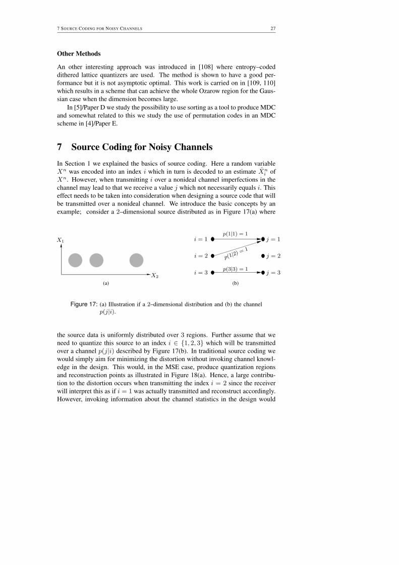
7 Source Coding for Noisy ChannelsIn Section 1 we explained the basics of source coding. Here a random variableXn was encoded into an index i which in turn is decoded to an estimate Xn

i ofXn. However, when transmitting i over a nonideal channel imperfections in thechannel may lead to that we receive a value j which not necessarily equals i. Thiseffect needs to be taken into consideration when designing a source code that willbe transmitted over a nonideal channel. We introduce the basic concepts by anexample; consider a 2–dimensional source distributed as in Figure 17(a) where

PSfrag replacements

X1

X2

(a)

PSfrag replacements

i = 1

i = 2

i = 3

j = 1

j = 2

j = 3

p(1|1) = 1

p(1|2)

= 1

p(3|3) = 1

(b)

Figure 17: (a) Illustration if a 2–dimensional distribution and (b) the channelp(j|i).

the source data is uniformly distributed over 3 regions. Further assume that weneed to quantize this source to an index i ∈ {1, 2, 3} which will be transmittedover a channel p(j|i) described by Figure 17(b). In traditional source coding wewould simply aim for minimizing the distortion without invoking channel knowl-edge in the design. This would, in the MSE case, produce quantization regionsand reconstruction points as illustrated in Figure 18(a). Hence, a large contribu-tion to the distortion occurs when transmitting the index i = 2 since the receiverwill interpret this as if i = 1 was actually transmitted and reconstruct accordingly.However, invoking information about the channel statistics in the design would

28 INTRODUCTIONPSfrag replacements

X1

X2

j = 1 j = 2 j = 3

i = 1 i = 2 i = 3

(a)

PSfrag replacements

X1

X2

j = 1

j = 2

j = 3

i = 1 i = 2 i = 3

(b)

Figure 18: Using the MSE distortion measure: (a) Encoder/decoder optimizedfor an ideal channel and (b) encoder/decoder optimized for the non-ideal channel of Figure 17(b).

make it possible to optimize the system better. This will enable the system to bet-ter protect itself against channel failures resulting in the design illustrated in Figure18(b) where a better overall MSE will be obtained than in the previous case. Notethat in the encoding we need to consider both how to design the quantization re-gions as well as the index assignment, i.e. how to label the quantization regionswith indices (changing the labelling affects the performance). The basic problemsof source coding with noisy channels are clear from this example: quantization,index assignment and decoding. These problems are discussed in the followingsections.

7.1 Scalar Source Coding for Noisy ChannelsThe first constructive work on scalar source coding for noisy channels was carriedout by Fine in [111]. Here a communication system with a discrete noisy channelis considered and rules for creating encoders as well as decoders are presented.This work continues in [112] where optimal quantizers and decoders are developedfor the case of binary channels, both for the unrestricted scalar quantizer as wellas for uniform quantizers. In [113] Farvardin and Vaishampayan extended thisresult to other channels and they also introduced a procedure to improve the indexassignment. These results are central in this topic and are summarized below.

PSfrag replacements

p(j|i)j

X Xi

f g

Figure 19: Model of a communication system.

The considered system is illustrated in Figure 19 where X is assumed to bean i.i.d. source and i ∈ {1, · · · ,M}. It is also assumed that MSE is used as a

7 SOURCE CODING FOR NOISY CHANNELS 29

distortion measure. For a fixed decoder g the encoder is created as

f(x) = arg mini

(

E[(x− X)2|I = i])

. (66)

This will result in optimal scalar quantizers for a given index assignment and agiven decoder g since it will consider the fact that X is a random variable. It is fur-ther shown that (66) can be developed such that the boarders of the optimal scalarquantizer can be found in an analytical fashion. Altogether, these two steps willimprove the performance of the encoder and the algorithm moves on to optimizethe decoder under the assumption that the encoder f is fixed. The optimal encoderis given by

g(j) = E[X|J = j]. (67)

These equations makes it possible to optimize the encoder and decoder in an iter-ative fashion and will result in a locally optimal solution for f and g, which notnecessarily equals the global optimal solution.

7.2 Vector Source Coding for Noisy ChannelsEarly works that can be categorized as vector source coding for noisy channelsinclude [114, 115] but the first more explicit work can be found in [116]. Hereoptimality conditions for encoders and decoders are formulated which results inchannel optimized vector quantization (COVQ). Also [117, 118] studies this sub-ject where [118] is good introduction to COVQ. The central results of these publi-cations are summarized for the MSE case. The system considered is basically thesame as in Figure 19 with X replaced by Xn and X replaced by Xn. For a fixeddecoder g the encoder should perform its vector quantization as

f(xn) = arg mini

(

E[(xn − Xn)2|I = i])

(68)

and for a fixed encoder f the decoder should be designed as

g(j) = E[Xn|J = j]. (69)

Also here the design is done by alternating between optimizing the encoder, (68),and the decoder, (69). Although the algorithm usually tends to converge to a goodsolution the initialization of the index assignment usually affects the performanceof the resulting design.

Further work is done in [119] where it is shown that once a COVQ system hasbeen designed the complexity is no greater than ordinary vector quantization. Thisindeed motivates the use of COVQ. However, just as in regular vector quantizationcomplexity will be an issue when the dimension and/or the rate is high. One solu-tion to this problem is to somehow restrict the structure of the quantization regionsby performing a multistage VQ, see e.g. [120, 121] for ideal channels and [122]for noisy channels. These quantizers will in general have a lower performance butalso a lower complexity.

30 INTRODUCTION

Soft Decoding

Most of the work done in joint source–channel coding uses a discrete channelmodel, p(jk|ik), arising from an analog channel in conjunction with a hard deci-sion scheme. This is illustrated in Figure 20 where ik is transmitted and distortedby the analog channel such that rk is received as

rk = ik + wk (70)

where wk is additive (real–valued) noise. This value is then converted to a discretevalue jk which results in a discrete channel model. However, if it is assumed

PSfrag replacements

p(jk|ik)

jk

wk

rk

Xn Xnikf g

Figure 20: Model of a channel arising from an analog channel in conjunctionwith a hard decision scheme

that the receiver can access and process the analog (or soft) values rk the decoderg could be based on rk, instead on jk. Since ik → rk → jk will constitute aMarkov chain we can conclude that rk will contain more, or possibly an equalamont of, information about ik than jk which means that decoding based on rk

should make it possible to get a better performance than decoding based on jk.For instance in the MSE case the optimal decoder is given as

Xn = E[Xn|Rk = rk]. (71)

Decoding based on soft channel values is often referred to as soft decodingand the idea originates from [123]. Further work is the area includes [124] whereHadamard–based optimal and suboptimal soft decoders are developed. In [125] ageneral treatment for soft decoding of noisy channels with finite memory is pro-vided. One of the main results is that the complex algorithms resulting from thistheory can be written in a recursive manner lowering the complexity. Also in [126]channels with memory is studied.

Using soft decoding results in a high decoding complexity. In [127, 128] thiscomplexity is decreased by quantizing the soft channel values. The quantizationproduces a vector jqk and is hence a compromise between using the complete softinformation rk and the commonly occurring coarse version, jk, of the informa-tion. The design criteria used is to design uniform scalar quantizers for the rm’ssuch that the mutual information between rm and jq

m is maximized. We furtherinvestigate how to create jqk by presenting a different approach in [3]/Paper G of

8 CONTRIBUTIONS OF THE THESIS 31

this thesis where theory for designing nonuniform quantizers are developed. Thesequantizers are optimal in the MSE sense.

7.3 Index AssignmentWhen dealing with noisy channels the index assignment of the different codewordsbecomes an important issue to consider. Otherwise, codewords that interchangefrequently may be far apart in the signal space which may cause a large contribu-tion to the distortion. However, the index assignment problem is NP-hard and tofind the optimal solution one would have to run a full search over the M ! possibleorderings of the M codevectors (although some of these permutations can be ruledout). Conducting a full search is not feasible in most practical situations whichhave made the research focus on suboptimal algorithms, with limited complexity,to solve the problem.

Early publications about the index assignment problem are [129, 130] whereheuristic algorithms are described. In [118, 131] simulated annealing is used togenerate good index assignments and in [132] a greedy method called “Pseudo–Gray Coding” is developed which is shown to have a good performance. In [133,134] the Hadamard transform is used as a tool to create, as well as to indicate theperformance of, index assignments for binary symetric channels. The method isdemonstrated to have a high performance and a fairly low complexity. This workis extended to cover more general channel models in [135].

8 Contributions of the ThesisIn this thesis we focus on four topics:

• Analog Bandwidth expansion. In Paper A we introduce and analyze a newanalog source–channel code based on orthogonal polynomials.

• Distributed source coding over noisy channels. In Papers B and C wepresent new joint source–channel schemes for distributed source coding overnonideal orthogonal channels.

• Multiple description coding. In papers D and E we introduce new MDCschemes. These schemes are analyzed as well as simulated. In paper Fwe improve the quantization in multiple description coding using pairwisecorrelation transforms, briefly explained in Section 6.2.

• Soft decoding. The main contribution in paper G is the study of how toquantize soft information for later use in a soft decision scheme.

The connections between these different topics and papers are illustrated in Fig-ure 21. MDC can be seen as a packet based expansion which makes this problemsomewhat similar to the analog bandwidth expansion problem. The same goes for

32 INTRODUCTION

PSfrag replacements

D–F, MDC

Packet based expansion

and packet loss

A, Bandwidth expansion

Analog expansion and

and noisy channel

G, Soft decoding

”Bit based expansion“

and noisy channel

B–C, Distributed coding

over orthogonal channels

Correlated sourcesand noisy channel

Figure 21: The connection between the different papers/topics in the thesis.

soft decoding, but here we transmit bits instead of packets and we can thereforethink of this situation as a kind of ”bit based expansion“. Finally, the bandwidthexpansion problem is a special case of distributed source coding over orthogonalchannels which will be discussed more in Paper C. The main contributions madein each paper are summarized below.

Paper A: Polynomial Based Analog Source–Channel Codes [12]

We study the problem of bandwidth expansion, i.e. when one source sample, X ,is transmitted over N orthogonal channels yielding a 1 : N expansion ratio. Ananalog source–channel code based on orthogonal polynomials is proposed and an-alyzed. Previous analog source-channel bandwidth expansion schemes have eitherfocused on a uniform source distribution or otherwise a general source distributionbut only for small N ’s. Our main contribution in this paper is that we produce acode for a large number of source distributions implementable also for large N ’s.The code can be generated using a Gram-Schmidt procedure, to fit virtually anysource distribution. By simulations we show that the performance is comparableto other existing schemes. However, the proposed scheme is more general and canbe implemented a larger class of source distributions.

8 CONTRIBUTIONS OF THE THESIS 33

Paper B: Distributed Quantization over Noisy Channels [10]

The problem of designing distributed quantizers for noisy channels is considered ina joint source–channel perspective. An algorithm for designing channel optimizeddistributed scalar quantizers for orthogonal channels is proposed and evaluated.The algorithm will produce a system operating on a sample by sample basis ina similar fashion as a channel optimized scalar quantizer (COSQ). In particularthe cases of the binary symmetric channel as well as the additive white Gaussiannoise channel are studied. It is demonstrated that the algorithm produces a wellworking system which is also robust against channel SNR mismatch. The workalso results in some interesting visualizations which clarifies the connection be-tween bandwidth expansion and distributed source coding over noisy channels.This connection is elaborated further in Paper C.

Paper C: Nonlinear Coding and Estimation for Correlated Data in WirelessSensor Networks [11]

Consider the problem when a number of sensors access noisy observations of a ran-dom source. These observations need to be communicated over orthogonal noisychannels to a final destination where the source value is estimated. We demon-strate similarities between this problem and the problem of bandwidth expansionwhich motivates the use of analog source–channel codes similar to what is used forbandwidth expansion. This results in nonlinear analog source–channel codes fordistributed estimation over noisy channels which are analyzed in a general setting.The conducted analysis reveals that there is a fundamental tradeoff when designinganalog source–channel codes for this problem: either one aims for combating thesensor observation noise which will make the system more sensitive to the channelnoise. On the other hand, if one instead would like to combat the channel noisethe system will become more sensitive to the observation noise.

Based on this understanding an explicit source–channel code is proposed, an-alyzed and simulated. One appealing property of the proposed scheme is that it isimplementable for many sources, contrary to most existing nonlinear distributedsource–channel coding systems.

Paper D: Sorting–based Multiple Description Quantization [5]

A new method for performing multiple description coding is introduced. Thescheme is based on sorting a frame of samples and transmitting, as side-information/redundancy, an index that describes the resulting permutation. In thecase that some of the transmitted descriptors are lost this side information (if re-ceived) can be used to estimate the lost descriptors based on the received ones.This can be done since the side information describes the order of the descriptorswithin the frame and hence each received descriptor will narrow down the possiblevalues of the lost ones. The side information is shown to be useful also in the case

34 INTRODUCTION

when no descriptors are lost. For the case of a uniform i.i.d. source a closed formexpression for the performance is derived making it possible to analytically opti-mize the choice of system parameters. Simulations conducted show the scheme tohave a similar performance to multiple description scalar quantization. The mainadvantage of the suggested method is that it has virtually zero design complexity,making it easy to implement and adapt to varying loss probabilities. It also has theadvantage of allowing straightforward implementation of high dimensional MDC.

Paper E: Multiple Description Coding using Rotated Permutation Codes [4]

The problem of designing multiple description source codes for J channels is ad-dressed. Our proposed technique consist mainly of two steps; first J copies ofthe vector Xn, containing the source data {xi}i=n

i=1 , are rotated by multiplicationof J random unitary matrices, i.e. one rotation matrix is generated and used foreach channel. Secondly each of the resulting vectors are, independently of theother vectors, vector quantized using permutation source coding. Furthermore, thedecoding of the received information when only one channel is received is doneby applying the inverse rotation to the result of standard permutation decoding;the optimum strategy for combining the information from multiple channels is amore difficult problem. Instead of implementing optimal combining we propose tosimply average the decoded output of the individual channels and then adjust thelength of the resulting vector based on a theoretical analysis valid for permutationcodes. The choice of using permutation codes comes from the fact that their lowcomplexity makes high dimensional vector quantization possible, i.e. large n’s,and our simulations have indicated that the random generation of rotation matricesworks well when the dimension is high. For low dimensions different outcomes ofthe generated rotation matrices seem to yield quite different performance, mean-ing that the random design may not be as appropriate for this case. Hence, anyvector quantization scheme able to perform quantization in high dimensions couldpotentially replace the permutation coding in the proposed scheme.

Using i.i.d. zero-mean Gaussian data for the xi’s we evaluated the proposedscheme by comparing it to multiple description scalar quantization (MDSQ) aswell as entropy-constrained MDSQ (ECMDSQ). It was shown that when usingJ = 2 and R = 4 bits/symbol the proposed system outperformed MDSQ. Com-pared to ECMDSQ a performance gain was achieved when optimizing the systemsfor receiving, close to, only one descriptor. Otherwise ECMDSQ had the betterperformance. The main advantages of the proposed method are its relatively lowcomplexity and its ability to easily implement any number of descriptions.

Paper F: Improved Quantization in Multiple Description Coding by Corre-lating Transforms [2]

Multiple description using pairwise correlation transforms (MDCPC) is studied.Here a pairwise correlating transforms introduces correlation between different

8 CONTRIBUTIONS OF THE THESIS 35

bitstreams. In the case of a lost bitstream, this correlation can be used in order toget an estimate of a lost stream. In this paper we suggest a new approach for per-forming the quantization in MDCPC. Using the original method the data is quan-tized and then transformed by a matrix operator in order to increase the redundancybetween descriptors. We suggest to reverse the order of these operations: first thedata is transformed and then quantized. We show that this leads to a modificationof the distortion measure. Using the generalized Lloyd algorithm when designingthe quantization codebook also leads to a new way to update the codevectors. Themodification makes it possible to improve the shape of the quantization cells and totailor these to the employed transform. Our simulations indicates that the modifiedmethod performs better than the original one when smaller amounts of redundancyare introduced into the transmitted data. For the simulations conducted the modi-fied method gave 2 dB signal–to–distortion gain compared to the original systemwhen no descriptors were lost. The gain decreased to about 0.5-1 dB when theprobability of lost descriptors was increased.

Paper G: On Source Decoding based on Finite–Bandwidth Soft Information[3]

Designing a communication system using joint source–channel coding in generalmakes it possible to achieve a better performance than when the source and channelcodes are designed separately, especially under strict delay-constraints. The ma-jority of work done in joint source-channel coding uses a discrete channel model,corresponding to an analog channel in conjunction with a hard decision scheme.The performance of such a system can however be improved by using soft decod-ing at the cost of a higher decoding complexity. An alternative is to quantize thesoft information and store the pre-calculated soft decision values in a lookup table.In this paper we propose new methods for quantizing soft channel information, tobe used in conjunction with soft-decision source decoding.

The issue on how to best construct finite-bandwidth representations of softinformation is further studied and compared for three main approaches: 1) re-quantization of the soft decoding estimate; 2) vector quantization of the soft chan-nel values, and; 3) scalar quantization of soft channel values. We showed analyt-ically that 1) and 2) are essentially equivalent. Also, since 3) is a special case of2) it can only yield similar or worse performance. However, we derived expres-sions that specify the optimal scalar quantizers, and when using designs based onthese a performance close to that of approaches 1) and 2) was achieved. The gainof this suboptimality is a substantially lower complexity which makes the methodinteresting.

36 INTRODUCTION

References[1] C. E. Shannon, “A mathematical theory of communication,” The Bell Systems Tech-

nical Journal, vol. 27, no. 3 and 4, pp. 379–423 and 623–656, July and Oct. 1948.

[2] N. Wernersson, T. Skollermo, and M. Skoglund, “Improved quantization in multi-ple description coding by correlating transforms,” in IEEE MMSP 2004, September2004.

[3] N. Wernersson and M. Skoglund, “On source decoding based on finite-bandwidthsoft information,” in Proceedings IEEE Int. Symp. Information Theory, September2005, pp. 87–91.

[4] ——, “Multiple description coding using rotated permutation codes,” in Data Com-pression Conference, March 2006.

[5] ——, “Sorting–based multiple description quantization,” IEEE Transactions onCommunications, vol. 54, no. 9, pp. 1521–1526, September 2006.

[6] J. Karlsson, N. Wernersson, and M. Skoglund, “Distributed scalar quantizers fornoisy channels,” in International Conference on Acoustics, Speech and Signal Pro-cessing (ICASSP), April 2007, pp. 633–636.

[7] N. Wernersson, J. Karlsson, and M. Skoglund, “Distributed scalar quantizers forgaussian channels,” in Proceedings IEEE Int. Symp. Information Theory, June 2007,pp. 1741–1745.

[8] P. A. Floor, T. A. Ramstad, and N. Wernersson, “Power constrained channel opti-mized vector quantizers used for bandwidth expansion,” in IEEE International Sym-posium on Wireless Communication Systems, October 2007.

[9] N. Wernersson, M. Skoglund, and T. Ramstad, “Analog source-channel codes basedon orthogonal polynomials,” in Asilomar Conference on Signals, Systems and Com-puters, November 2007.

[10] N. Wernersson, J. Karlsson, and M. Skoglund, “Distributed quantization over noisychannels,” IEEE Transactions on Communications, 2008, to appear.

[11] N. Wernersson and M. Skoglund, “Nonlinear coding and estimation for correlateddata in wireless sensor networks,” IEEE Transactions on Communications, 2008,submitted.

[12] N. Wernersson, M. Skoglund, and T. Ramstad, “Polynomial based analog source–channel codes,” IEEE Transactions on Communications, 2008, submitted.

[13] A. Eskicioglu and P. Fisher, “Image quality measures and their performance,” IEEETransactions on Information Theory, vol. 43, no. 12, pp. 2959–2965, dec 1995.

[14] T. M. Cover and J. A. Thomas, Elements of Information Theory. Wiley-Interscience,1991.

[15] T. S. Han and S. Verdu, “Approximation theory of output statistics,” IEEE Transac-tions on Information Theory, vol. 39, no. 3, pp. 752–772, May 1993.

[16] A. Gersho and R. M. Gray, Vector Quantization and Signal Compression. Dor-drecht, The Netherlands: Kluwer academic publishers, 1992.

[17] R. M. Gray and D. L. Neuhoff, “Quantization,” IEEE Transactions on InformationTheory, vol. 44, no. 6, pp. 2325–2383, October 1998.

REFERENCES 37

[18] D. Slepian, “Permutation modulation,” Proc. IEEE, vol. 53, pp. 228–236, March1965.

[19] J. Dunn, Coding for continuous sources and channels, Ph.D. dissertation. ColumbiaUniv., New York, 1965.

[20] T. Berger, F. Jelinek, and J. Wolf, “Permutation codes for sources,” IEEE Transac-tions on Information Theory, vol. 18, no. 1, pp. 160–169, January 1972.

[21] T. Berger, “Optimum quantizers and permutation codes,” IEEE Transactions on In-formation Theory, vol. 18, no. 6, pp. 759–765, November 1972.

[22] V. Goyal, S. Savari, and W. Wang, “On optimal permutation codes,” IEEE Transac-tions on Information Theory, vol. 47, no. 7, pp. 2961–2971, November 2001.

[23] R. L. Dobrushin, “General formulation of Shannon’s main theorem of informationtheory,” Usp. Math. Nauk., 1959, translated in Am. Math. Soc. Trans., 33:323-438.

[24] S. Vembu, S. Verdu, and Y. Steinberg, “The source-channel separation theorem revis-ited,” IEEE Transactions on Information Theory, vol. 41, no. 1, pp. 44–54, January1995.

[25] S. Verdu and T. S. Han, “A general formula for channel capacity,” IEEE Transactionson Information Theory, vol. 40, no. 4, pp. 1147–1157, July 1994.

[26] S. Vembu, S. Verdu, and Y. Steinberg, “When does the source-channel separationtheorem hold?” in Proceedings IEEE Int. Symp. Information Theory, June 1994, p.198.

[27] M. Gastpar, B. Rimoldi, and M. Vetterli, “To code, or not to code: lossy source-channel communication revisited,” IEEE Transactions on Information Theory,vol. 49, no. 5, pp. 1147–1158, May 2003.

[28] M. Skoglund, N. Phamdo, and F. Alajaji, “Hybrid digital-analog source-channel cod-ing for bandwidth compression/expansion,” IEEE Transactions on Information The-ory, vol. 52, no. 8, pp. 3757–3763, August 2006.

[29] C. E. Shannon, “Communication in the presence of noise,” Proc. IRE, pp. 10–21,January 1949.

[30] J. Ziv, “The behavior of analog communications systems,” IEEE Transactions onInformation Theory, vol. 16, no. 5, pp. 587–594, September 1970.

[31] D. J. Sakrison, Transmission of Waveforms and Digital Information. Wiley, 1968.

[32] V. Goyal, M. Vetterli, and N. Thao, “Quantized overcomplete expansions in Rn:

analysis, synthesis, and algorithms,” IEEE Transactions on Information Theory,vol. 44, pp. 16–31, January 1998.

[33] U. Timor, “Design of signals for analog communication,” IEEE Transactions on In-formation Theory, vol. 16, no. 5, pp. 581–587, September 1970.

[34] D. D. McRay, “Performance evaluation of a new modulation technique,” IEEE Trans-actions on Information Theory, vol. 19, no. 4, pp. 431–445, August 1971.

[35] V. Vaishampayan and S. I. R. Costa, “Curves on a sphere, shift-map dynamics, anderror control for continuous alphabet sources,” IEEE Transactions on InformationTheory, vol. 49, no. 7, pp. 1658–1672, July 2003.

38 INTRODUCTION

[36] B. Chen and G. W. Wornell, “Analog error-correcting codes based on chaotic dynam-ical systems,” IEEE Transactions on Communications, vol. 46, no. 7, pp. 881–890,July 1998.

[37] M. Taheradeh and A. K. Khandani, “Robust joint source-channel coding for delay-limited applications,” in Proceedings IEEE Int. Symp. Information Theory, June2007, pp. 726–730.

[38] A. Fuldseth and T. A. Ramstad, “Bandwidth compression for continuous amplitudechannels based on vector approximation to a continuous subset of the source sig-nal space,” in International Conference on Acoustics, Speech and Signal Processing(ICASSP), Munich, Germany, April 1997, pp. 3093–3096.

[39] S. Y. Chung, “On the construction of some capacity-approaching coding schemes,”Ph.D. dissertation, MIT, 2000.

[40] J. Karlsson and M. Skoglund, “Joint source-channel mappings for the relay chan-nel,” in Proceedings IEEE International Conference on Acoustics, Speech, and Sig-nal Processing, April 2008.

[41] S. S. Pradhan, J. Kusuma, and K. Ramchandran, “Distributed compression in a densemicrosensor network,” IEEE Signal Processing Magazine, vol. 19, no. 2, pp. 51–60,March 2002.

[42] Z. Xiong, A. D. Liveris, and S. Cheng, “Distributed source coding for sensor net-works,” IEEE Signal Processing Magazine, vol. 21, no. 5, pp. 80–94, September2004.

[43] B. Girod, A. M. Aaron, S. Rane, and D. Rebollo-Monedero, “Distributed video cod-ing,” Proceedings of the IEEE, vol. 93, no. 1, pp. 71–83, January 2005.

[44] D. Slepian and J. K. Wolf, “Noiseless coding of correlated information sources,”IEEE Transactions on Information Theory, vol. IT-19, no. 4, pp. 471–480, July 1973.

[45] A. D. Wyner and J. Ziv, “The rate-distortion function for source coding with sideinformation at the decoder,” IEEE Transactions on Information Theory, vol. IT-22,no. 1, pp. 1–10, January 1976.

[46] A. D. Wyner, “The rate-distortion function for source coding with side information atthe decoder-ii: General sources,” Information and Control, vol. 38, pp. 60–80, 1978.

[47] A. Wyner, “Recent results in the shannon theory,” IEEE Transactions on InformationTheory, vol. 20, no. 1, pp. 2–10, January 1974.

[48] S. S. Pradhan and K. Ramchandran, “Distributed source coding using syndromes(DISCUS): design and construction,” IEEE Transactions on Information Theory,vol. 49, no. 3, pp. 626–643, March 2003.

[49] A. D. Liveris, Z. Xiong, and C. N. Georghiades, “Compression of binary sourceswith side information at the decoder using LDPC codes,” IEEE CommunicationsLetters, vol. 6, no. 10, pp. 440–442, October 2002.

[50] J. Garcia-Frias and Y. Zhao, “Compression of correlated binary sources using turbocodes,” IEEE Commnications Letters, vol. 5, no. 10, pp. 417–419, October 2001.

[51] Z. Xiong, A. Liveris, S. Cheng, and Z. Liu, “Nested quantization and Slepian-Wolfcoding: a Wyner-Ziv coding paradigm for i.i.d. sources,” in IEEE Workshop on Sta-tistical Signal Processing, September 2003, pp. 399–402.

REFERENCES 39

[52] S. Pradhan and K. Ramchandran, “Generalized coset codes for distributed binning,”IEEE Transactions on Information Theory, vol. 51, no. 10, pp. 3457–3474, October2005.

[53] T. J. Flynn and R. M. Gray, “Encoding of correlated observations,” IEEE Transac-tions on Information Theory, vol. 33, no. 6, pp. 773–787, November 1987.

[54] W.M. Lam and A. R. Reibman, “Design of quantizers for decentralized estimationsystems,” IEEE Transactions on Communications, vol. 41, no. 11, pp. 1602–1605,November 1993.

[55] D. Rebollo-Monedero, R. Zhang, and B. Girod, “Design of optimal quantizers fordistributed source coding,” in Proc. IEEE Data Compression Conf., March 2003, pp.13–22.

[56] E. Tuncel, “Predictive coding of correlated sources,” in IEEE Information TheoryWorkshop, October 2004, pp. 111–116.

[57] M. Fleming, Q. Zhao, and M. Effros, “Network vector quantization,” IEEE Transac-tions on Information Theory, vol. 50, no. 8, pp. 1584– 1604, August 2004.

[58] A. Saxena and K. Rose, “Distributed predictive coding for spatio-temporally corre-lated sources,” in Proceedings IEEE Int. Symp. Information Theory, June 2007, pp.1506–1510.

[59] J. J. Xiao and Z. Q. Luo, “Multiterminal source-channel communication over anorthogonal multiple-access channel,” IEEE Transactions on Information Theory,vol. 53, no. 9, pp. 3255–3264, September 2007.

[60] B. Liu and B. Chen, “Channel-optimized quantizers for decentralized detection insensor networks,” IEEE Transactions on Information Theory, vol. 52, no. 7, pp.3349–3358, July 2006.

[61] A. Saxena, J. Nayak, and K. Rose, “On efficient quantizer design for robust dis-tributed source coding,” in Proceedings IEEE Data Compression Conference, March2006, pp. 63–71.

[62] S. Cui, J. Xiao, A. Goldsmith, Z. Luo, and V. Poor, “Estimation diversity and energyefficiency in distributed sensing,” IEEE Transactions on Signal Processing, vol. 55,no. 9, pp. 4683–4695, September 2007.

[63] Z. Luo, G. Giannakis, and S. Zhang, “Optimal linear decentralized estimation in abandwidth constrained sensor network,” in Proceedings IEEE Int. Symp. InformationTheory, September 2005, pp. 1441–1445.

[64] M. Gastpar and M. Vetterli, “Source-channel communication in sensor networks,” inProc. 2nd Int. Workshop Information Processing in Sensor Networks (IPSN03) (Lec-ture Notes in Computer Science), L. J. Guibas and F. Zhao, Eds. Berlin, Germany:Springer-Verlag, 2003, pp. 162–177.

[65] M. Gastpar, “Uncoded transmission is exactly optimal for a simple gaussian ”sensor”network,” in Proc. 2nd Annu. Workshop on Information Theory and its Applications,,January 2007, pp. 177–182.

[66] T. Berger and Z. Zhang, “Minimum breakdown degradation in binary source en-coding,” IEEE Transactions on Information Theory, vol. 29, no. 6, pp. 807–814,November 1983.

40 INTRODUCTION

[67] A. E. Gamal and T. Cover, “Achievable rates for multiple descriptions,” IEEE Trans-actions on Information Theory, vol. 28, no. 6, pp. 851–857, November 1982.

[68] L. Ozarow, “On a source coding problem with two channels and three receivers,”Bell Syst. Tech. J., vol. 59, no. 10, pp. 1909–1921, December 1980.

[69] R. Ahlswede, “The rate-distortion region for multiple descriptions without excessrate,” IEEE Transactions on Information Theory, vol. 31, no. 6, pp. 721–726,November 1985.

[70] Z. Zhang and T. Berger, “New results in binary multiple descriptions,” IEEE Trans-actions on Information Theory, vol. 33, no. 4, pp. 502–521, July 1987.

[71] R. Zamir, “Gaussian codes and shannon bounds for multiple descriptions,” IEEETransactions on Information Theory, vol. 45, no. 7, pp. 2629–2636, November 1999.

[72] L. A. Lastras-Montano and V. Castelli, “Near sufficiency of random coding for twodescriptions,” IEEE Transactions on Information Theory, vol. 52, no. 2, pp. 681 –695, February 2006.

[73] R. Venkataramani, G. Kramer, and V. Goyal, “Multiple description coding with manychannels,” IEEE Transactions on Information Theory, vol. 49, no. 9, pp. 2106–2114,September 2003.

[74] S. Pradhan, R. Puri, and K. Ramchandran, “n-channel symmetric multipledescriptions-part i:(n, k)source-channel erasure codes,” IEEE Transactions on In-formation Theory, vol. 50, no. 1, pp. 47–61, January 2004.

[75] R. Puri, S. Pradhan, and K. Ramchandran, “n-channel symmetric multipledescriptions-part ii:an achievable rate-distortion region,” IEEE Transactions on In-formation Theory, vol. 51, no. 4, pp. 1377–1392, April 2005.

[76] D. Slepian and J. Wolf, “Noiseless coding of correlated information sources,” IEEETransactions on Information Theory, vol. 19, no. 4, pp. 471–480, July 1973.

[77] A. Wyner and J. Ziv, “The rate-distortion function for source coding with side infor-mation at the decoder,” IEEE Transactions on Information Theory, vol. 22, no. 1, pp.1–10, January 1976.

[78] R. Ahlswede, “On multiple descriptions and team guessing,” IEEE Transactions onInformation Theory, vol. 32, no. 4, pp. 543–549, July 1986.

[79] F. Fang-Wei and R. W. Yeung, “On the rate-distortion region for multiple descrip-tions,” IEEE Transactions on Information Theory, vol. 48, no. 7, pp. 2012–2021,July 2002.

[80] V. K. Goyal, “Multiple description coding: Compression meets the network,” IEEESignal Processing Magazine, vol. 18, pp. 74–93, sep 2001.

[81] V. A. Vaishampayan, “Design of multiple description scalar quantizers,” IEEE Trans-actions on Information Theory, vol. 39, no. 3, pp. 821–834, 1993.

[82] V. A. Vaishampayan and J. Domaszewicz, “Design of entropy-constrained multiple-description scalar quantizers,” IEEE Transactions on Information Theory, vol. 40,pp. 245–250, January 1994.

[83] P. A. Chou, T. Lookabaugh, and R. M. Gray, “Entropy-constrained vector quantiza-tion,” IEEE Transactions on Signal Processing, vol. 37, no. 1, pp. 31–42, January1989.

REFERENCES 41

[84] V. A. Vaishampayan and J. C. Batllo, “Asymptotic analysis of multiple descriptionquantizers,” IEEE Transactions on Information Theory, vol. 44, no. 1, pp. 278–284,January 1998.

[85] C. Tian and S. S. Hemami, “Universal multiple description scalar quantization: anal-ysis and design,” IEEE Transactions on Information Theory, vol. 50, no. 9, pp. 2089–2102, September 2004.

[86] J. Balogh and J. A. Csirik, “Index assignment for two-channel quantization,” IEEETransactions on Information Theory, vol. 50, no. 11, pp. 2737–2751, November2004.

[87] T. Y. Berger-Wolf and E. M. Reingold, “Index assignment for multichannel commu-nication under failure,” IEEE Transactions on Information Theory, vol. 48, no. 10,pp. 2656–2668, October 2002.

[88] S. D. Servetto, V. A. Vaishampayan, and N. J. A. Sloane, “Multi description latticevector quantization,” in Proceedings IEEE Data Compression Conference, Snow-bird, UT, March 1999, pp. 13–22.

[89] V. A. Vaishampayan, N. J. A. Sloane, and S. D. Servetto, “Multiple description vectorquantization with lattice codebooks: Design and analysis,” IEEE Transactions onInformation Theory, vol. 47, no. 5, pp. 1718–1734, 2001.

[90] M. Fleming and M. Effros, “Generalized multiple description vector quantization,”in Proceedings IEEE Data Compression Conference, March 1999, pp. 3–12.

[91] N. Gortz and P. Leelapornchai, “Optimization of the index assignments for multi-ple description vector quantizers,” IEEE Transactions on Communications, vol. 51,no. 3, pp. 336–340, March 2003.

[92] P. Koulgi, S. Regunathan, and K. Rose, “Multiple description quantization by deter-ministic annealing,” IEEE Transactions on Information Theory, vol. 49, no. 8, pp.2067 – 2075, August 2003.

[93] S. N. Diggavi, N. J. A. Sloane, and V. A. Vaishampayan, “Asymmetric multipledescription lattice vector quantizers,” IEEE Transactions on Information Theory,vol. 48, no. 1, pp. 174–191, January 2002.

[94] V. A. Vaishampayan, A. R. Calderbank, and J. C. Batllo, “On reducing granulardistortion in multiple description quantization,” in Proceedings IEEE Int. Symp. In-formation Theory, August 1998, p. 98.

[95] V. K. Goyal, J. A. Kelner, and J. Kovacevic, “Multiple description vector quantizationwith a coarse lattice,” IEEE Transactions on Information Theory, vol. 48, no. 3, pp.781–788, March 2002.

[96] Y. Wang, M. Orchard, and A. Reibman, “Multiple description image coding for noisychannels by pairing transform coefficients,” in Proc. IEEE 1997 1st Workshop Mul-timedia Signal Processing (MMSP’97), Princeton, NJ, jun 1997, pp. 419–424.

[97] M. T. Orchard, Y. Wang, V. A. Vaishampayan, and A. R. Reibman, “Redundancyrate-distortion analysis of multiple description coding using pairwise correlatingtransforms,” in Proc. IEEE International Conference on Image Processing, 1997,pp. 608 – 611.

42 INTRODUCTION

[98] Y. Wang, M. Orchard, V. Vaishampayan, and A. Reibman, “Multiple description cod-ing using pairwise correlation transforms,” IEEE Transactions on Image Processing,vol. 10, no. 3, March 2001.

[99] Y. Wang, A. Reibman, M. Orchard, and H. Jafarkhani, “An improvement to multipledescription transform coding,” IEEE Transactions on Signal Processing, vol. 50,no. 11, November 2002.

[100] V. K. Goyal and J. Kovacevic, “Generalized multiple description coding with cor-relating transforms,” IEEE Transactions on Information Theory, vol. 47, no. 6, pp.2199–2224, sep 2001.

[101] S. S. Pradhan and K. Ramchandran, “On the optimality of block orthogonal trans-forms for multiple description coding of gaussian vector sources,” IEEE Signal Pro-cessing Letters, vol. 7, no. 4, pp. 76 – 78, April 2000.

[102] F. J. MacWilliams and N. J. A. Sloane, The Theory of Error-Correcting Codes. Am-sterdam: North-Holland, 1977.

[103] V. K. Goyal, J. Kovacevic, and M. Vetterli, “Multiple description transform coding:Robustness to erasures using tight frame expansion,” in Proceedings IEEE Int. Symp.Information Theory, Cambridge, MA, August 1998, p. 408.

[104] ——, “Quantized frame expansions as source-channel codes for erasure channels,”in Proceedings IEEE Data Compression Conference, Snowbird, UT, March 1999,pp. 326–335.

[105] V. K. Goyal, J. Kovacevic, and J. A. Kelner, “Quantized frame expansions with era-sures,” Applied and Computational Harmonic Analysis, vol. 10, no. 3, pp. 203 – 233,May 2001.

[106] J. Kovacevic, P. L. Dragotti, and V. K. Goyal, “Filter bank frame expansions witherasures,” IEEE Transactions on Information Theory, vol. 48, no. 6, pp. 1439 – 1450,June 2002.

[107] S. M. Kay, Fundamentals of Statistical Signal Processing: Estimation Theory. Pren-tice Hall, 1993.

[108] Y. Frank-Dayan and R. Zamir, “Dithered lattice-based quantizers for multiple de-scriptions,” IEEE Transactions on Information Theory, vol. 48, no. 1, pp. 192 – 204,January 2002.

[109] J. Chen, C. Tian, T. Berger, and S. S. Hemami, “A new class of universal multipledescription lattice quantizers,” in Proceedings IEEE Int. Symp. Information Theory,September 2005, pp. 1803 – 1807.

[110] ——, “Multiple description quantization via gram-schmidt orthogonalization,” IEEETransactions on Information Theory, vol. 52, no. 12, pp. 5197–5217, December2006.

[111] T. Fine, “Properties of an optimum digital system and applications,” IEEE Transac-tions on Information Theory, vol. IT-10, pp. 443–457, October 1964.

[112] A. Kurtenbach and P. Wintz, “Quantizing for noisy channels,” IEEE Trans. Commun.Techn., vol. COM-17, pp. 291–302, April 1969.

[113] N. Farvardin and V. Vaishampayan, “Optimal quantizer design for noisy channels:An approach to combined source–channel coding,” IEEE Transactions on Informa-tion Theory, vol. 33, no. 6, pp. 827–838, November 1987.

REFERENCES 43

[114] J. G. Dunham and R. M. Gray, “Joint source and noisy channel trellis encoding,”IEEE Transactions on Information Theory, vol. 27, no. 4, pp. 516–519, July 1981.

[115] J. D. Gibson and T. R. Fischer, “Alphabeth-constrained data compression,” IEEETransactions on Information Theory, vol. 28, no. 3, pp. 443–457, May 1982.

[116] H. Kumazawa, M. Kasahara, and T. Namekawa, “A construction of vector quantizersfor noisy channels,” Electronics and engineering in Japan, vol. 67-B, pp. 39–47,January 1984.

[117] K. A. Zeger and A. Gersho, “Vector quantizer design for memoryless noisy chan-nels,” in IEEE Internationell Conference on Communications, Philadelphia, USA,1988, pp. 1593–1597.

[118] N. Farvardin, “A study of vector quantization for noisy channels,” IEEE Transactionson Information Theory, vol. 36, no. 4, pp. 799–809, July 1990.

[119] N. Farvardin and V. Vaishampayan, “On the performance and complexity of channel-optimized vector quantizers,” IEEE Transactions on Information Theory, vol. 37,no. 1, pp. 155–159, January 1991.

[120] B. Juang and A. Gray, “Multiple stage vector quantization for speech coding,” inProceedings IEEE International Conference on Acoustics, Speech, and Signal Pro-cessing, May 1982.

[121] W. Y. Chan, S. Gupta, and A. Gersho, “Enhanced multistage vector quantization byjoint codebook design,” IEEE Transactions on Communications, vol. 40, no. 11, pp.1693–1697, November 1992.

[122] N. Phamdo, N. Farvardin, and T. Moriya, “A unified approach to tree-structured andmultistage vector quantization for noisy channels,” IEEE Transactions on Informa-tion Theory, vol. 39, no. 3, pp. 835–850, May 1993.

[123] V. Vaishampayan and N. Farvardin, “Joint design of block source codes and mod-ulation signal sets,” IEEE Transactions on Information Theory, vol. 38, no. 4, pp.1230–1248, July 1992.

[124] M. Skoglund and P. Hedelin, “Hadamard-based soft decoding for vector quantizationover noisy channels,” IEEE Transactions on Information Theory, vol. 45, no. 2, pp.515–532, March 1999.

[125] M. Skoglund, “Soft decoding for vector quantization over noisy channels with mem-ory,” IEEE Transactions on Information Theory, vol. 45, no. 4, pp. 1293–1307, May1999.

[126] N. Phamdo, F. Alajaji, and N. Farvardin, “Quantization of memoryless and Gauss-Markov sources over binary Markov channels,” IEEE Transactions on Communica-tions, vol. 45, no. 6, pp. 668–675, June 1997.

[127] F. Alajaji and N. Phamdo, “Soft-decision COVQ for Rayleigh fading channels,”IEEE Communications Letters, vol. 2, no. 6, pp. 162–164, June 1998.

[128] N. Phamdo and F. Alajaji, “Soft-decision demodulation design for COVQ over white,colored and ISI Gaussian channels,” IEEE Transactions on Communications, vol. 48,no. 9, pp. 1499–1506, September 2000.

[129] K. A. Zeger and A. Gersho, “Zero redundancy channel coding in vector quantiza-tion,” IEE Electronic Letters, vol. 23, no. 12, pp. 654–655, June 1987.

44 INTRODUCTION

[130] J. DeMarca and N. Jayant, “An algorithm for assigning binary indices to the codevec-tors of a multi-dimensional quantizer,” in IEEE Internationell Conference on Com-munications, Seattle, USA, 1987, pp. 1128–1132.

[131] D. J. Goodman and T. J. Moulsley, “Using simmulated annealing to design digitaltransmission codes for analogue sources,” IEE Electronic Letters, vol. 24, no. 10, pp.617–619, May 1988.

[132] K. A. Zeger and A. Gersho, “Pseudo-Gray coding,” IEEE Transactions on Commu-nications, vol. 38, no. 12, pp. 2147–2158, December 1990.

[133] P. Knagenhjelm and E. Agrell, “The Hadamard transform — A tool for index assign-ment,” IEEE Transactions on Information Theory, vol. 42, no. 4, pp. 1139–1151,July 1996.

[134] R. Hagen and P. Hedelin, “Robust vector quantization by a linear mapping of a blockcode,” IEEE Transactions on Information Theory, vol. 45, no. 1, pp. 200–218, Jan-uary 1999.

[135] M. Skoglund, “On channel constrained vector quantization and index assignment fordiscrete memoryless channels,” IEEE Transactions on Information Theory, vol. 45,no. 7, pp. 2615–2622, November 1999.

Part II

Included papers

Paper A

Polynomial Based Analog Source–Channel Codes

Niklas Wernersson, Mikael Skoglund and Tor RamstadSubmitted to IEEE Transactions of Communications

Polynomial Based Analog Source–Channel Codes

Niklas Wernersson, Mikael Skoglund and Tor Ramstad

Abstract

In many communication applications one is interested in transmitting a time-discreteanalog-valued (i.e. continuous alphabet) source over a time-discrete analog channel. Westudy this problem in the case of bandwidth expansion, in the sense that one source sample,X , is transmitted over N orthogonal channels. An analog source–channel code based onorthogonal polynomials is proposed and analyzed. The code can be generated using aGram-Schmidt procedure, to fit virtually any source distribution.

Index Terms–Modulation, nonlinear functions, source coding, channel coding, errorcorrection.

1 IntroductionWe consider the problem of analog bandwidth expansion over a Gaussian memoryless chan-nel. This means designing analog source–channel bandwidth expansion codes where asource sample X is transmitted using an AWGN channel N times, yielding a 1 : N ex-pansion rate. (We will from now on refer to these codes as ’analog source–channel codes’.)The common solution for this problem is digital and is implemented by producing sepa-rate source and channel codes. In practice, this is generally done by quantizing the sourcefollowed by digital channel coding and transmission. Due to powerful source and channelcoding techniques the performance of such a system can be very high when the channelquality is close to what the system has been designed for. There are, however, some disad-vantages with the digital approach. In order to get a high performance long block lengthsare required both for the source and channel code. This will therefore introduce delays intothe system which may be undesirable, especially for a real time system. There is also athreshold effect associated with a digital system: if the channel quality goes below a cer-tain level the channel code will break down and the system performance will deterioraterapidly. On the other hand, if the channel quality is increased above this level the perfor-mance will not increase but rather reach a constant level which is due to the nonrepairableerrors introduced by the quantizer.

In recent years analog, or at least partially analog, systems as an alternative to digitalsystems have received increased attention, see e.g. [1, 2] and the references therein. Analogsystems do, in general, not have the same disadvantages as digital systems. Hence, in somescenarios an analog approach may be more suitable than a digital one. On the other hand, in

A2 POLYNOMIAL BASED ANALOG SOURCE–CHANNEL CODESPSfrag replacements

x

......

...

s1(x)r1

w1

s2(x)r2

w2

sN (x)rN

wN

x

Figure 1: Structure of the system.

practice, the performance of a digital system is in general higher than for an analog systemwhen being used for the channel quality that it has been designed for.

Analog bandwidth expansion was briefly discussed already in one of Shannon’s earlypapers [5]. Furthermore [6] analyzes the performance of analog source–channel codes athigh SNR’s. The papers [7–9] present ideas for how to construct these codes and in [10, 11]it is concluded that the problem also relates to the problem of distributed estimation. How-ever, to our knowledge, the only more explicit results on how to design analog source–channel codes are found in [2–4]. In all these papers a uniform source distribution is con-sidered.

Our main contribution in this paper, which was partly presented in [12], is to presenta method for designing well-performing analog source–channel codes assuming a generalsource distribution.

The paper is organized as follows. In Section 2 the problem is formulated. Section 3provides a brief introduction to orthogonal polynomials. Section 4 will propose an analogsource–channel code and Section 5 will present some analytical results for this code. Finallywe present some simulation results and conclusions in Sections 6-7.

2 Problem FormulationConsider the problem illustrated in Figure 1. An analog source value x, with variance σ2

x

and pdf f(x), is encoded by the function

s(x) = (s1(x), s2(x), . . . , sN (x))T (1)

and transmitted over N orthogonal AWGN channels created by using e.g. TDMA or FDMA.The different encoding functions perform analog mappings, that is si : R → R, under thepower constraints

E[si(X)2] =

�R

f(x)si(x)2dx ≤ P ∀i ∈ {1, 2, . . . , N}. (2)

The decoder estimates x based on the received values

r = s(x) + w (3)

2 PROBLEM FORMULATION A3

where w is independent and identically distributed (i.i.d.) memoryless Gaussian distributedwith covariance matrix σ2

wI . Hence, the decoding is performed as

x = x(r) (4)

and the objective is to minimize the expected mean square error (MSE) E[(X − X)2].When the source is i.i.d. zero-mean Gaussian and N = 1, it is well known that lin-

ear encoding is optimal, i.e. s1(x) = � (P/σ2x)x, under the assumption that the decoder

knows the source and noise variances. However, when N > 1 this is no longer true andnonlinear encoding can have superior performance compared to linear encoding strategies,see e.g. [13]. One of the reasons for this is that a linear encoding function s(x) only usesa one dimensional subspace of the channel space. More efficient mappings would use ahigher number of the available channel space dimensions. An example of this is illustratedin Figure 2 for N = 2. By using nonlinear encoding functions, illustrated by the solid’S-shaped’ curve s(x), we are able to better fill the channel space than when using linearencoding functions, represented by the dashed curve. A longer curve essentially means ahigher resolution when estimating x as long as we decode to the right fold of the curve, il-lustrated by sample x1 in the figure. However, decreasing the SNR will at some point resultin that different folds of the curve will lie too close to each other and the decoder will startmaking large decoding errors, illustrated by sample x2 in the figure. Decreasing the SNRbelow this threshold will therefore significantly deteriorate the performance. We refer tothese errors as ’small’ and ’large’ decoding errors. Increasing the SNR, on the other hand,will always improve the performance since the magnitude of the small decoding errors willdecrease. This is one of the main advantages of analog systems compared to digital systemssince the performance of a digital system will approach a saturation level when the SNRgrows large.

The problem of designing analog source–channel codes is therefore a problem of find-ing nonlinear curves s(x) : R → R

N under the power constraints (2) such that points farseparated in the source space also are far separated in the channel space, i.e.

‖s(x) − s(x + δ)‖2 > ∆2 ∀{(x, δ) : f(x) > 0, |δ| > δ0} (5)

where ∆ and δ0 are some positive constants. If this condition is true, no large (the valueof δ0 will define “large”) decoding errors will occur if the probability of noise vectors2‖w‖2 > ∆2 can be neglected, see e.g. [14]. This will be true when the SNR reachesabove some certain threshold. Furthermore, given that no large coding errors occur theexpected MSE will only depend on the small decoding errors. In [15] it is shown that underthese conditions the MSE will depend on the stretch of s(x) defined as

S(x) = ���� d

dxs(x) ���� , (6)

which preferably should be as large as possible. The expected MSE is then well approxi-mated by

E[(X − X)2] = σ2w

�R

f(x)

‖ ddx

s(x)‖2dx. (7)

To summarize, we would like to ’stretch’ the curve s(x) as much as possible underthe constraints in (2) and (5). We will in this paper design such curves using orthogonalpolynomials.

A4 POLYNOMIAL BASED ANALOG SOURCE–CHANNEL CODES

PSfrag replacements

s1(x)

s2(x)

w1 r1

s(x1)

s(x1)

w2

r2

s(x2)

s(x2)

Figure 2: x1 illustrates a ’small’ decoding error and x2 illustrates a ’large’ de-coding error.

3 Orthogonal PolynomialsThe orthogonal polynomials literature is vast, see e.g. [16, 17] for an introduction to thearea. We will here summarize some important results which will be used in the followingsections.

3.1 DefinitionA sequence of polynomials {Pn(x)}∞n=0 is called orthogonal with respect to the weightfunction f(x) if Pn(x) is a polynomial of degree n and for all non-negative n and m�

R

f(x)Pn(x)Pm(x)dx = δnmKn, Kn 6= 0 (8)

where δnm is Kronecker’s delta symbol. Furthermore, if Kn = 1 ∀n the sequence ofpolynomials {Pn(x)}∞n=0 is orthonormal. We will use the notation pn(x) when referringto orthonormal polynomials, hence

pn(x) = � 1/KnPn(x). (9)

3.2 The recurrence formula and zerosIt can be shown that given a sequence of orthogonal polynomials {Pn(x)}∞n=0 there existconstants cn and λn such that

Pn(x) = (x − cn)Pn−1(x) − λnPn−2(x), n > 0 (10)

where P0(x) = 1 and P−1(x) = 0. These constants will depend of the weight functionf(x). The zeros of Pn(x) are real and simple. We will denote the k:th smallest zero of

3 ORTHOGONAL POLYNOMIALS A5

−1.5 −1 −0.5 0 0.5 1 1.5−2

−1.5

−1

−0.5

0

0.5

1

1.5

2

PSfrag replacements

x

pn(x

)

p5(x)

p20(x)

p100(x)

Figure 3: Orthonormal polynomials for a Gaussian source (σ2 = 0.5).

Pn(x) as xk,n. It can be shown that the zeros of Pn(x) and Pn+1(x) mutually separateeach other such that

xk,n+1 < xk,n < xk+1,n+1, k = 1, 2, . . . , n. (11)

These properties explain the well known fact that orthogonal polynomials have an oscil-lating behavior, see e.g. [18]. Due to that all zeros of Pn(x) are real and simple we canwrite

Pn(x) ∝ (x − x1,n)(x − x2,n) · · · (x − xn,n), (12)

meaning that as x increases Pn(x) will alternate sign when the different zeros are passed.In fact, the polynomial Pn(x) usually behave quite similar to a sine if studied in a fairlyshort interval where f(x) is strong, at least when n grows large. This is illustrated in Figure3 where orthonormal polynomials for a Gaussian source with variance 0.5 is plotted. As itturns out, the oscillating property will be important for our proposed analog source–channelcode.

3.3 Gram–SchmidtGiven a weight function f(x) ≥ 0 orthonormal polynomials {pn(x)}∞n=0 will exist. Thesepolynomials can be derived by a Gram–Schmidt procedure described briefly below.

1. Set P0(x) = 1 and create p0(x) from (9). Set n = 0.

2. Create

Pn+1(x) = xn+1 −n�

k=0

akpk(x) (13)

where by choosing

ak =

�R

f(x)xn+1pk(x)dx (14)

A6 POLYNOMIAL BASED ANALOG SOURCE–CHANNEL CODES

it is ensured that Pn+1(x) is orthogonal to {pl(x)}nl=0 since�

R

f(x)Pn+1(x)pl(x)dx =

�R

f(x)xn+1pl(x)dx −�

R

f(x)

n�k=0

akpk(x)pl(x)dx

= al − al = 0 (15)

if l < n + 1.

3. Create pn+1(x) by (9) and set n = n + 1. Go to Step 2.

Hence, given a certain pdf f(x) the procedure above will produce the corresponding or-thonormal polynomials.

3.4 The Christoffel–Darboux identityFinally we state the Christoffel–Darboux identity,

N�n=0

pn(x)pn(u) = � KN+1

KN

pN+1(x)pN (u) − pN (x)pN+1(u)

x − u. (16)

4 Encoding and DecodingWe propose a nonlinear analog source–channel code as follows. Given I ={i1, i2, . . . , iN} the analog source–channel code sI(x) is created by choosing

sj(x) =√

Ppij (x) ∀j ∈ {1, 2, . . . , N}. (17)

For example, given a source distribution f(x) and I = {1, 2, 3, 4} we will use√

Pp1(x)as encoding function for the first channel,

√Pp2(x) for the second channel and so on. Here

the pn(x)’s are orthonormal with respect to the weight function f(x). Hence, the weightfunction equals the source pdf meaning that the power constraint in (2) will be fulfilledsince

E[sj(X)2] =

�R

f(x)[√

Ppij (x)]2dx = P. (18)

Optimal decoding, in the minimum MSE sense, is given as [19]

x(r) = E[x|r] (19)

but this decoding function would be very complex to implement. We therefore choose toinstead implement the suboptimal maximum likelihood decoder

x(r) = arg maxx

g(r|x) = arg minx

‖sI(x) − r‖2 = arg minx �� �

ij∈I

(√

Ppij (x) − rj)2 �� ,

(20)

5 ANALYSIS A7

where g(·|·) denotes the channel transition pdf. Hence, the decoding procedure is equivalentto minimizing a 2iN -degree polynomial (assuming iN is the largest index in I). Efficient al-gorithms exist for minimizing univariate polynomials which makes this feasible.1 It shouldbe emphasized that (20), i.e. the receiver, does not need to know σ2

w .Finally, note that the special case IL , {1, 1, . . . , 1} means that the encoding is linear

as discussed in Section 2 and in Figure 2. We will later use this system as a benchmarksystem.

5 AnalysisWe will here discuss the three desirable properties for analog source–channel codes dis-cussed in Section 2: A) distance properties as in (5), B) stretch properties as in (7) andfinally, C) the ability to use up to all available channel space dimensions. We will showthat the proposed scheme possesses properties A and C and we further conjecture that italso possesses property B for a large class of pdf:s f(x). For such pdf:s the suggestedscheme will therefore procedure a working source–channel code which consequently canbe generated using the Gram–Schmidt procedure from Section 3.

5.1 DistanceAssume that four consecutive orthonormal polynomials are used as an analog source–channel code, hence I = {n − 3, n − 2, n − 1, n}. We will here show that this implies(5).

Proof : If (5) is not valid for some x and |δ| > 0 we have ‖sI(x) − sI(x + δ)‖ = 0meaning Pi(x) = Pi(x + δ) for i ∈ I. If we use this in the recurrence equation (10) weget

Pn(x + δ) = (x + δ − cn)Pn−1(x + δ) − λnPn−2(x + δ)

and hence

Pn(x) = (x − cn)Pn−1(x) + δPn−1(x) − λnPn−2(x).

Comparing this last equation with (10) we realize that this can be true only if: i) δ = 0 orii) Pn−1(x) = 0. Hence, x must equal one of Pn−1(x)’s zeros xk,n−1. Repeating thisderivation for polynomials {n − 3, n − 2, n − 1} and studying x = xk,n−1 we get

Pn−1(xk,n−1) =(xk,n−1 − cn−1)Pn−2(xk,n−1) + δPn−2(xk,n−1) − λn−1Pn−3(xk,n−1).

Hence, also Pn−2(xk,n−1) needs to equal 0 which can not be true according to (11). Hence,there can be no point where sI(x) = sI(x+δ) if |δ| > 0 and I = {n−3, n−2, n−1, n}meaning that ∆2 > 0 will exist such that (5) is fulfilled. �

In Figure 4 we illustrate the distance properties for a few different I’s by plotting thefunction ‖sI(x) − sI(x0)‖2 in the case of a uniform source distribution, i.e. f(x) = 1/2for x ∈ (−1, 1). All these codes have appropriate distance properties.

1It should here be pointed out that when simulating the scheme for large iN ’s our computer’s defaultaccuracy for float values was not high enough making the minimization procedure to fail due to roundoff errors. This therefore needed to be considered. For our simulations in Section 6 the effect becamevisible for iN ’s somewhere between 20 and 25.

A8 POLYNOMIAL BASED ANALOG SOURCE–CHANNEL CODES

−1 −0.5 0 0.5 10

1

2

3

4

5

6

x

PSfrag replacements ‖sI(x

)−

sI(1

/3)‖

2

I1I2I3

Figure 4: The distance ‖sI(x) − sI(x0)‖2 for I1 = {1, 2, 3, 4, 5, 6}, I2 ={1, 2, 5, 6, 17, 18} and I3 = {1, 2, . . . , 1000} when x0 = 1/3. Thepowers have been normalized so that each channel uses P = 1/N .Similar results were obtained also when other values for x0 are cho-sen.

5.2 StretchGiven that the SNR is high the MSE is well approximated by (7). We conjecture that givena smooth and continuous f(x) for I = {1, 2, · · · , N}, where N is large enough, we have�

R

f(x)

‖ ddx

sI(x)‖2dx <

�R

f(x)

‖ ddx

sIL(x)‖2

dx. (21)

In fact, for all the different f(x):s we have evaluated, for instance the ones in the Section 6,the inequality has been true already for N = 2. Consequently, for high SNR’s the proposedcode will produce a better MSE than a linear code.

5.3 DimensionsAs earlier commented on a weakness with the linear code sIL

(x) is that only a one dimen-sional subspace of the channel space is used for transmission. We will here show that givenf(xk,iN +1) 6= 0 ∀k and I = {i1, i2, . . . , iN} where i1 < i2 < · · · < iN all dimensionsin the channel space will be used.

Proof : If we use I = {0, 1, . . . , iN} to create the (iN + 1) × (iN + 1) matrix

A = [sI(x1,iN +1) sI(x2,iN +1) · · · sI(xiN +1,iN +1)]

all columns will be orthogonal. This comes from the fact that the right-hand-side of (16)will always equal 0 if x = xi,iN +1 and u = xj,iN +1 and i 6= j. The left-hand-side of (16)

6 SIMULATIONS A9

describes the dot product of column vectors i and j in A which hence are orthogonal. Thisfurther means that A is full rank. If we instead create the matrix

A = [sI(x1,iN +1) sI(x2,iN +1) · · · sI(xiN +1,iN +1)]

it is a version of A where a number of rows are removed. Since A is full rank also A willbe full rank. Hence, sI(x) will use all N available dimensions in the channel space fortransmission since we have assumed f(xk,iN +1) 6= 0 ∀k. �

To summarize, the curve sI(x) is not contained in a subspace of the N -dimensionalchannel space.

6 Simulations6.1 Choosing IIn Section 5 we motivated that orthogonal polynomials have properties making them appro-priate as analog source–channel codes as proposed in Section 4. However, the question onhow to choose which indexes to include in I remains. We will here present a strategy forthis based on results derived in [2]. Only the case with symmetric pdf’s will be consideredand we will leave the asymmetric case as a future topic.

As discussed in Section 3 orthonormal polynomials have an oscillating property. In thissense our proposed scheme is similar to the scheme in [2] where sine and cosine functionswith different frequencies are used to create analog source–channel codes for a uniformlydistributed source x ∈ (−1, 1). Furthermore, [2] carries out a rigorous analysis in order tooptimize the choice of which frequencies to use which leads to the encoding structure

s1+2i(x) = α cos(πaix)s2+2i(x) = α sin(πaix) ∀i ∈ {0, 1, . . . , N/2 − 1} (22)

where a ∈ N. It is shown that a higher a leads to a higher stretch but also that different foldsof the curve is packed closer to each other. If we study (s1(x), s2(x)) we note that this pairof functions will create a circle in the plane when x is increased from −1 to 1. Furthermore,for (s1+2i(x), s2+2i(x)) the same behavior is obtained with the difference that the functionwill go ai laps around the circle. Our proposed structure will approximate this behavior if

I = {2a0 − 1, 2a0, 2a1 − 1, 2a1, 2a2 − 1, 2a2, . . .}. (23)

This comes from the fact that p2ak (x) will have 2ak zeros and hence ak ’periods’ (oscilla-tions) before the polynomial starts approaching ±∞. Due to the distribution of zeros (11)there will exist ’phase shifts’ between pi(x) and pi+1(x) and we can roughly think of everyother polynomial as a sine and every other as a cosine, at least for symmetric pdf’s. Thecurve (p2ai−1(x), p2ai(x)) will therefore approximate the circles created by the system in(22). This is illustrated in Figure 5 where (p49(X), p50(X)) have been simulated for 50000Gaussian source samples X , darker points in the plot means more occurring points. Mostof the source samples are mapped to an area approximately looking like a circle around theorigin although we also note that the samples in the tails of the pdf f(x) will be mappedto regions further out. Therefore the results obtained in [2] motivates the choice of I as in(23). This choice has also been supported by simulations conducted where other choices ofI have been evaluated.

A10 POLYNOMIAL BASED ANALOG SOURCE–CHANNEL CODES

0

0

PSfrag replacements

p49(X)

p50(X

)

Figure 5: p49(x) versus p50(x) simulated for a Gaussian source. The darkerpoint, the more occurrences.

6.2 Optimal companding and benchmark systems

As previously noted, to our knowledge, the only existing schemes of analog source–channelcodes are [2–4] which all are designed for a uniform distribution. We will use [2, 3] asbenchmark systems and from now on refer to these as the V&C and C&W codes. A weak-ness with these is that s(−1) = s(1). Hence, they are sensitive for large decoding errorswhen transmitting values close to the ends of the support region for the distribution. Thisis solved by instead encoding βx, rather than x, where β is some appropriate constant lessthan 1 in order to prevent large decoding errors. However, this property makes it hard to nat-urally extend the ideas to other distributions, for instance the Gaussian distribution whichdoes not have a limited support. This was briefly commented on in [2] and it was sug-gested that optimal companding, see e.g. [15], could be used in conjunction with the codesin order to create codes for other distributions. In order to get some benchmark systemsfor nonuniform sources we therefore use optimal companding together with the V&C andC&W codes. The compander will map the source x to y(x) ∈ (−1, 1) and then transmits(y(x)).2 From [15] we get the optimal compander, in the minimum MSE sense, as

y(x) = 2 x

−∞f(u)

13 du ∞−∞ f(u)13 du

− 1. (24)

The receiver will estimate y and the inverse companding operation is performed such thatx is found fulfilling y = y(x).

2Since y(x) produced by the compander not is uniformly distributed the individual power con-straints of (2) will be violated. We allow this and instead require the total power consumption to be lessthan NP for the benchmark systems.

6 SIMULATIONS A11

6.3 ResultsIn order to evaluate the proposed code we carried out simulations for three different sourcedistributions: Uniform, Gaussian and a Gaussian mixture (GM). The pdf’s for these can bewritten

fU (x) = 1/2 x ∈ (−1, 1)

fG(x, σ2) =1√

2πσ2exp(− x2

2σ2)

fGM (x, σ2) =�

i

qifG(x − µi, σ2)

where we used σ2 = 0.5 for the Gaussian case. This results in two of the most famousorthogonal polynomials for the Uniform and Gaussian source, namely the Legendre andHermite polynomials which both are well documented and explicit formulas for the poly-nomials exists. For the GM distribution we used σ2 = 1, q = 1/6 · [1, 1, 2, 1, 1] andµ = [−7,−4, 0, 4, 7] which is not a well documented weight function. Therefore this sim-ulation tested the usefulness of the Gram–Schmidt procedure from Section 3 which wasused to generate the corresponding analog source–channel code.

In Figure 6 simulation results are presented for the case of 1 : 6 expansion. Performanceis measured in terms of 1/MSE versus SNR per channel, i.e. SNR , P/σ2

w . All curvesshow similar behavior, for low SNR’s large decoding errors occur and the performance islow. Increasing the SNR from this point leads to an increase in performance and eventuallythe threshold where large decoding errors stop occurring is reached and the performancestarts behaving according to (7).

Figure 1.6(a) shows results for the uniform source. This is the case for which both theV&C and C&W codes were constructed. We experienced that the V&C code perform betterthan our proposed scheme. It appears as if when the stretch for both codes are chosen suchthat the performance is similar above the threshold the V&C code reaches its threshold at alower SNR than our code. The C&W code on the other hand is quite far behind in terms ofperformance. The slope of the performance curve for the C&W code is on the other handsteeper which was also explained in [3]. The linear code, sIL

(x), is the best choice onlyfor very bad channels.

In Figure 1.6(b) the Gaussian source is simulated and optimal companding has beenimplemented for the V&C and C&W codes. The companding (24) and the inverse com-panding operations, which for this case can be expressed in terms of the Q–function, willnaturally add complexity. Here the proposed scheme has the superior performance.

Finally, in Figure 1.6(c) we have also simulated the GM source. Deriving the com-panding integral (24) for this pdf is difficult and we can therefore only compare to linearcoding. From the figure we see that the Gram–Schmidt generated polynomials producesa well working analog source–channel code. This illustrates the power of the proposedscheme and the Gram–Schmidt procedure in order to design analog source–channel codesfor general distributions.

A12 POLYNOMIAL BASED ANALOG SOURCE–CHANNEL CODES

−10 −5 0 5 10 15 20 25 30 350

10

20

30

40

50

60

70

80

LinearC&W

V&C

PSfrag replacements

sI

SNR [dB] per channel

1/

MSE

[dB

]

(a) Uniform

−10 −5 0 5 10 15 20 25 30 35−10

0

10

20

30

40

50

60

70

LinearC&W

V&C

PSfrag replacements

sI

SNR [dB] per channel

1/

MSE

[dB

]

(b) Gaussian

−10 −5 0 5 10 15 20 25 30 35−20

−10

0

10

20

30

40

Linear

PSfrag replacements

sI

SNR [dB] per channel

1/

MSE

[dB

]

(c) Gaussian mixture

Figure 6: Simulations for different source distributions. In (a)–(b) we use a ∈{3, 4} for V&C and a ∈ {4, 5} for sI(x). In (c) we use a ∈ {2, 5}for sI(x).

7 CONCLUSIONS A13

7 ConclusionsWe have presented an analog source-channel coding scheme for bandwidth expansion anda Gram-Schmidt procedure for generating the code for a general source has been described.The scheme has a similar performance to the the best previous existing scheme but is moregeneral and can be implemented for a larger class of source distributions.

References[1] M. Skoglund, N. Phamdo, and F. Alajaji, “Hybrid digital-analog source-channel cod-

ing for bandwidth compression/expansion,” IEEE Transactions on Information The-ory, vol. 52, no. 8, pp. 3757–3763, August 2006.

[2] V. Vaishampayan and S. I. R. Costa, “Curves on a sphere, shift-map dynamics, and er-ror control for continuous alphabet sources,” IEEE Transactions on Information The-ory, vol. 49, no. 7, pp. 1658–1672, July 2003.

[3] B. Chen and G. W. Wornell, “Analog error-correcting codes based on chaotic dynam-ical systems,” IEEE Transactions on Communications, vol. 46, no. 7, pp. 881–890,July 1998.

[4] M. Taheradeh and A. K. Khandani, “Robust joint source-channel coding for delay-limited applications,” in Proceedings IEEE Int. Symp. Information Theory, June 2007,pp. 726–730.

[5] C. E. Shannon, “Communication in the presence of noise,” Proc. IRE, pp. 10–21,January 1949.

[6] J. Ziv, “The behavior of analog communications systems,” IEEE Transactions on In-formation Theory, vol. 16, no. 5, pp. 587–594, September 1970.

[7] U. Timor, “Design of signals for analog communication,” IEEE Transactions on In-formation Theory, vol. 16, no. 5, pp. 581–587, September 1970.

[8] D. D. McRay, “Performance evaluation of a new modulation technique,” IEEE Trans-actions on Information Theory, vol. 19, no. 4, pp. 431–445, August 1971.

[9] P. A. Floor, T. A. Ramstad, and N. Wernersson, “Power constrained channel optimizedvector quantizers used for bandwidth expansion,” in IEEE International Symposiumon Wireless Communication Systems, October 2007.

[10] N. Wernersson, J. Karlsson, and M. Skoglund, “Distributed quantization over noisychannels,” IEEE Transactions on Communications, 2008, to appear.

[11] N. Wernersson and M. Skoglund, “Nonlinear coding and estimation for correlated datain wireless sensor networks,” IEEE Transactions on Communications, 2008, submit-ted.

[12] N. Wernersson, M. Skoglund, and T. Ramstad, “Analog source-channel codes basedon orthogonal polynomials,” in Asilomar Conference on Signals, Systems and Com-puters, November 2007.

[13] J. M. Wozencraft and I. M. Jacobs, Principles of Communication Engineering. Wiley,1965.

A14 POLYNOMIAL BASED ANALOG SOURCE–CHANNEL CODES

[14] L. P. Seidman, “An upper bound on average estimation error in nonlinear systems,”IEEE Transactions on Information Theory, vol. 14, no. 2, pp. 243–250, March 1968.

[15] D. J. Sakrison, Transmission of Waveforms and Digital Information. Wiley, 1968.

[16] T. S. Chihara, An introduction to orthogonal polynomials. Mathematics and its Ap-plications, 1978.

[17] G. Szego, Orthogonal polynomials, 4th ed. American Mathematical Society, 1975.

[18] A. Mate, P. Nevai, and V. Totik, “Oscillatory behavior of orthogonal polynomials,”Proceedings of the American Mathematical Society, vol. 96, no. 2, pp. 261–268,February 1986.

[19] S. M. Kay, Fundamentals of Statistical Signal Processing: Estimation Theory. Pren-tice Hall, 1993.

Paper B

Distributed Quantization over Noisy Channels

Niklas Wernersson, Johannes Karlsson and Mikael SkoglundTo appear in IEEE Transactions of Communications

Distributed Quantization over Noisy Channels

Niklas Wernersson, Johannes Karlsson and Mikael Skoglund

Abstract

The problem of designing simple and energy-efficient sensor nodes in a wireless sensornetwork is considered from a joint source–channel coding perspective. An algorithm for de-signing distributed scalar quantizers for orthogonal channels is proposed and evaluated. Inparticular the cases of the binary symmetric channel as well as the additive white Gaussiannoise channel are studied. It is demonstrated that correlation between sources can be usefulin order to reduce quantization distortion as well as protecting data when being transmittedover non-ideal channels. It is also demonstrated that the obtained system is robust againstchannel SNR mismatch.

Index Terms–Source coding, quantization, channel coding, correlation.

1 IntroductionWireless sensor networks are expected to play an important role in tomorrow’s sensingsystems. One important property in these networks is that there may be a high correlationbetween different sensor measurements due to high spatial density of sensor nodes. Thismotivates source coding of correlated sources, which has been analyzed in for instance [1]where the well known Slepian–Wolf theorem is stated. Ideas on how to perform practicalSlepian–Wolf coding are presented in [2, 3], allowing the use of powerful channel codessuch as LDPC and Turbo codes in the context of distributed source coding, see e.g. [4, 5].For the case with continuous sources, i.e. lossy coding, relevant references include [6, 7].In general, these methods require the use of long codes and the encoding complexity willrequire some data processing in the sensor nodes. This will therefore counteract one ofthe desired design criteria in sensor network design, namely low cost and energy efficientsensor nodes. In addition, in many applications for example in networked control, a lowdelay is essential, preventing the use of long codes.

An alternative is therefore to design sensor nodes of very low complexity and low delay.This can be accomplished by interpreting the distributed source coding problem as a quan-tization problem. Previously, quantization of correlated sources has been studied in [8–13].Our work is however targeted towards wireless sensor networks and introducing noisy chan-nels is necessary in order to make the system more realistic. For non-ideal channels relatedprevious work includes [14] which considers the problem of distributed detection over non-ideal channels. In [15] quantization of correlated sources in a packet network is studied,

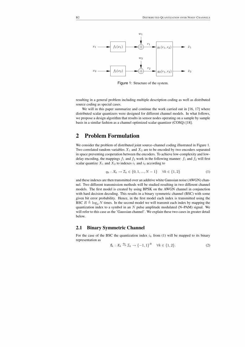
B2 DISTRIBUTED QUANTIZATION OVER NOISY CHANNELSPSfrag replacements

x1 f1(x1)

w1

r1

x2 f2(x2)

w2

r2

x1

x2

g1(r1, r2)

g2(r1, r2)

Figure 1: Structure of the system.

resulting in a general problem including multiple description coding as well as distributedsource coding as special cases.

We will in this paper summarize and continue the work carried out in [16, 17] wheredistributed scalar quantizers were designed for different channel models. In what follows,we propose a design algorithm that results in sensor nodes operating on a sample by samplebasis in a similar fashion as a channel optimized scalar quantizer (COSQ) [18].

2 Problem FormulationWe consider the problem of distributed joint source–channel coding illustrated in Figure 1.Two correlated random variables X1 and X2 are to be encoded by two encoders separatedin space preventing cooperation between the encoders. To achieve low-complexity and low-delay encoding, the mappings f1 and f2 work in the following manner: f1 and f2 will firstscalar quantize X1 and X2 to indexes i1 and i2 according to

qk : Xk → Ik ∈ {0, 1, ..., N − 1} ∀k ∈ {1, 2} (1)

and these indexes are then transmitted over an additive white Gaussian noise (AWGN) chan-nel. Two different transmission methods will be studied resulting in two different channelmodels. The first model is created by using BPSK on the AWGN channel in conjunctionwith hard decision decoding. This results in a binary symmetric channel (BSC) with somegiven bit error probability. Hence, in the first model each index is transmitted using theBSC R , log2 N times. In the second model we will transmit each index by mapping thequantization index to a symbol in an N pulse amplitude modulated (N–PAM) signal. Wewill refer to this case as the ’Gaussian channel’. We explain these two cases in greater detailbelow.

2.1 Binary Symmetric ChannelFor the case of the BSC the quantization index ik from (1) will be mapped to its binaryrepresentation as

fk : Xkqk→ Ik → {−1, 1}R ∀k ∈ {1, 2}. (2)

2 PROBLEM FORMULATION B3

Hence, fk will use qk to create the index ik which is then represented binary. These bits aretransmitted over a Gaussian channel using BPSK resulting in

rk = fk(xk) + wk ∀k ∈ {1, 2} (3)

where w is zero mean i.i.d. Gaussian noise with covariance matrix σ2wI. For each of these

R received values a hard decision decoding rule is applied such that

jk(m) = sign(rk(m)) m = 1, 2, · · · , R (4)

where

sign(x) = � 1, x ≥ 0−1, x < 0.

(5)

Given that −1 was transmitted, and letting Q(·) denote the Q-function, this will result in abit error probability

ε =

� ∞0

1√2πσ2

w

e−

(r+1)2

2σ2w dr = Q � 1

σw , (6)

which is also, due to the symmetry, the total bit error probability.Denoting the decimal representation of jk as jk the decoding will be performed as

xk = gk(j1, j2) ∀k ∈ {1, 2}. (7)

Hence, the decoding is based on both j1 and j2.Given this system, we define the mean squared error (MSE) as

D =1

2(D1 + D2) =

1

2 � E[(X1 − X1)2] + E[(X2 − X2)

2] � (8)

and our objective is to design the encoders and the decoder in order to minimize the MSE.1

2.2 Gaussian ChannelFor the Gaussian channel each of the indexes (i1, i2) are mapped to an N pulse amplitudemodulated (N–PAM) signal such that

fk(xk) = α(2qk(xk) − N + 1) ∀k ∈ {1, 2}. (9)

Here α is a constant such that the power constraints

E[fk(Xk)2] ≤ P ∀k ∈ {1, 2} (10)

are satisfied. The two PAM signals are then transmitted over two orthogonal channels,created by using e.g. TDMA or FDMA, resulting in the received values

rk = fk(xk) + wk ∀k ∈ {1, 2} (11)

1As pointed out by one of the reviewers one could also define a weighted MSE as D(ρ) = ρD1 +(1−ρ)D2 and adopt our derived equations accordingly. One interesting case would be D(1) meaningthat the second observation x2 only serves as side information when estimating x1. However, we willonly study the case D(0.5), i.e. as in (8).

B4 DISTRIBUTED QUANTIZATION OVER NOISY CHANNELS

where the noise terms wk are independent zero-mean Gaussian distributed with varianceσ2

w . The decoder will have access to both r1 and r2 and forms its estimate of the originalsource data as

xk = gk(r1, r2) ∀k ∈ {1, 2}. (12)

Here the objective is to design the encoders and the decoder in order to minimize the MSEfrom (8) under the power constraints given in (10).

3 AnalysisAs in traditional Lloyd-Max training [19] we will optimize each part in the system in aniterative fashion keeping the other parts fixed. Note that the system contains three parts:two encoders and one decoder, although the decoder contains two decoding functions. Wewill in this section consider the design of these parts under the assumption that

Xk = Y + Zk ∀k ∈ {1, 2} (13)

where Y , Z1 and Z2 are independent zero-mean Gaussian distributed random variables withvariances σ2

Y , σ2Z1

= σ2Z2

= σ2Z . Hence, X1 and X2 are correlated which can be exploited

in the encoding as well as the decoding.For this jointly Gaussian distribution we get the conditional pdf

p(x2|x1) =1√

2πσ2exp ��� − � x2 − σ2

Y

σ2Y

+σ2Z

x1 � 2

2σ2 ���� (14)

where

σ2 =σ4

Z + 2σ2Y σ2

Z

σ2Y + σ2

Z

. (15)

Without loss of generality we will further assume that E[X21 ] = E[X2

2 ] = 1, hence σ2Y +

σ2Z = 1.

3.1 Encoder for BSCOnly the design of f1 will be considered since f2 can be designed in the same fashion. Giventhat the encoder f1 observes x1 and produces index i1 it can derive the expected distortionsfor D1 and D2 as

D1(x1, i1) =�j1

�j2

P (j1|i1)P (j2|x1) [x1 − g1(j1, j2)]2 (16)

D2(x1, i1) =

� �j1

�j2

P (j1|i1)p(x2|x1)P (j2|q2(x2)) [x2 − g2(j1, j2)]2 dx2, (17)

where the integral is taken from −∞ to ∞ and

P (j2|x1) =�i2

P (j2|i2)P (i2|x1) (18)

3 ANALYSIS B5

whereP (i2|x1) =

�x2:q2(x2)=i2

p(x2|x1)dx2. (19)

The other transition probabilities P (·|·) are straightforward to derive, see e.g. [20]. In orderto minimize the distortion (8) the quantizer q1(x1) should be designed according to

q1(x1) = arg mini1

(D1(x1, i1) + D2(x1, i1)). (20)

In [18] the case of a single source was studied. In this case, the solution resulted inencoder regions which were intervals, and analytical expressions for finding the endpointsof these intervals were derived. However, (20) does in general not result in a similar solutionand the encoder regions will in general not be intervals, but rather unions of separatedintervals (this will be illustrated in Section 4).

3.2 Encoder for Gaussian ChannelFor the Gaussian channel D1 and D2 can be expressed as

D1(x1, i1) =

���p(r1|i1)p(r2|x1) [x1 − g1(r1, r2)]

2 dr2dr1 (21)

D2(x1, i1) =

�����p(r1|i1)p(x2|x1)p(r2|q2(x2)) [x2 − g2(r1, r2)]

2 dr2dx2dr1, (22)

where the integrals are taken from −∞ to ∞. In order to minimize the distortion (8) underthe power constraint (10) the quantizer q1(x1) should be designed according to

q1(x1) = arg mini1

(D1(x1, i1) + D2(x1, i1) + λ(2i1 − N + 1)2). (23)

Here, the first two terms aim at minimizing the distortion introduced by the quantizerwhereas the third term will allow us to control the power consumption by choosing a valuefor the Lagrangian multiplier λ, see e.g. [21]. Unfortunately the integrals in (21)–(22) aredifficult to evaluate since they contain g1(r1, r2) and g2(r1, r2) which vary with r1 andr2. In order to get around this problem we use the technique of prequantizing r1 and r2

according toh : (R1,R2) → (J1,J2) ∈ {1, 2, ..., M}2 (24)

which will produce the decoding functions

xk = gk(h(r1, r2)) = gk(j1, j2) ∀k ∈ {1, 2}. (25)

Furthermore, in this work we choose M = N and let h(r1, r2) simply map (r1, r2) to theclosest possible output from the encoders defined by (f1(x1), f2(x2)). Hence

h(r1, r2) = arg min(j1,j2)

((r1 − α(2j1 − N + 1))2 + (r2 − α(2j2 − N + 1))2). (26)

The decoding functions will now be piecewise linear over r1 and r2 which greatly sim-plifies the derivation of (21–22) and we get the same equations as in (16–17) (although thetransition probabilities are different). Using (23) together with (16–17) will therefore definethe optimal quantizer q1(x1) under the assumption that the decoder and the second encoderare fixed.

B6 DISTRIBUTED QUANTIZATION OVER NOISY CHANNELS

3.3 DecoderAssuming fixed encoders it is a well known fact from estimation theory that the optimal, inminimum MSE sense, estimates of x1 and x2 are given as

xk = gk(j1, j2) = E[xk | j1, j2] ∀k ∈ {1, 2}. (27)

Hence, (27) is used to derive the decoders for both considered transmission methods.

3.4 Design algorithmBased on the developed equations (20), (23) and (27) it will be possible to optimize theencoders and the decoder. A natural order to optimize these is : 1) the first encoder, 2) thedecoder, 3) the second encoder, 4) the decoder. Each step in the iteration will guarantee thedistortion to decrease and the training is repeated until the solution converges. Just as in thecase of the Lloyd-Max algorithm this will result in a locally optimal system which is notnecessarily the global optimum.

One problem with the suggested training above is that the obtained local optimum pro-duced will depend greatly on the initialization of the decoder and encoders. In fact, inour simulations we experienced that very poor local optima were often found using the ap-proach suggested above. This problem has also been encountered in [18, 22–24] where themethod of noisy channel relaxation was introduced. The idea is essentially that it is easier tofind a good local optimum for channels with high noise energy than for channels with lownoise energy. Therefore a system is first designed for a very bad channel. Next, the channelquality is gradually improved and a new system is designed in each step. For each design,a full iterative training algorithm is executed using the reconstruction codebook from theprevious design as initialization for the current design. We incorporate this idea by startingdesigning a system for a noise variance σ′2w � σ2

w . When this is completed σ′2w is decreasedwith a stepsize σ2

∆ and a new system is designed. This is repeated L times. The algorithmis summarized below.

1. Initialize encoders and optimize the decoder by using (27).2. Set values for L and σ2

∆. Create σ′2w = σ2w + Lσ2

∆.3. Design a system for the channel noise σ′2w according to:

(a) Set the iteration index k = 0 and D(0) = ∞.(b) Set k = k + 1.(c) Find the optimal quantizer q1 by using (20) (or (23)).(d) Find the optimal decoder by using (27).(e) Find the optimal quantizer q2 by using q2(x2)’s equivalence to (20) (or (23)).(f) Find the optimal decoder by using (27).(g) Evaluate the distortion D(k) for the system. If the relative improvement of

D(k) compared to D(k−1) is less than some threshold δ > 0 go to Step 4.Otherwise go to Step (b).

4. If σ′2w = σ2w stop the iteration. Otherwise create σ′2w = σ′2w − σ2

∆ and go to Step 3using the current encoders and decoder when initializing the next iteration.

We also experienced that when searching for a good local optima a small improvement wassometimes obtained by also performing a noise relaxation procedure for the correlation,i.e. varying σ2

z . However, the main improvement was obtained by the algorithm above.

4 SIMULATIONS B7

3.5 Optimal Performance Theoretically AttainableRecently the rate region for the quadratic two-terminal source coding problem has beencompletely characterized in [25]. Furthermore, in [26] it is shown that separating the sourceand channel code design, when the block lengths are approaching infinity, will be asymptot-ically optimal for the problem we are considering. Hence, by simply studying the channelcapacity of the different orthogonal channels we get rate constraints, R1 and R2, on thesource code since these rates can be safely communicated to the decoder. Assuming thatwe have access to a capacity achieving channel code for the BSC we get

βBSC = R1 = R2 = RCBSC = R(1 + ε log2 ε + (1 − ε) log2(1 − ε)) (28)

where CBSC is the capacity of the BSC [27]. For the Gaussian channel we note that bothencoders have the same power constraint (10) and that both channels have the same noisepower. This gives

βAWGN = R1 = R2 = CAWGN =1

2log2 � 1 +

P

σ2w (29)

where CAWGN is the capacity of the AWGN channel [27]. Using the appropriate β, from (28)or (29), and simplifying the expressions in [25] (remember the assumption σ2

Y + σ2Z = 1)

givesD1D2 ≥ 2−4β(1 − σ4

Y ) + σ4Y 2−8β . (30)

Since D1 is inversely proportional to D2 the total distortion in (8) will be minimized bysetting D = D1 = D2. This gives the optimal performance theoretically attainable (OPTA)according to

D = � 2−4β(1 − σ4Y ) + σ4

Y 2−8β . (31)

That is, D in (31) is the lowest possible achievable distortion for this problem.

4 SimulationsWe will here visualize the structure of the encoders obtained when using the design algo-rithm presented in Section 3.4. The performance of a designed system is also compared tothe OPTA derived in Section 3.5. In order to do so we measure the signal-to-distortion ratio(SDR) defined as

SDR = 10 log10 � E[X21 ] + E[X2

2 ]

E[(X1 − X1)2] + E[(X2 − X2)2] (32)

and we also define the correlation SNR as

CSNR = 10 log10 � σ2Y

σ2Z . (33)

Hence, CSNR = −∞ dB means that X1 and X2 are uncorrelated and CSNR = ∞ dBmeans that they are fully correlated. We use the term SNR when referring to the channelSNR defined as 10 log10(P/σ2

w). As initial encoders we used uniform quantizers and forthe case of BSC the folded binary code [28] was used as initial codeword assignment.

B8 DISTRIBUTED QUANTIZATION OVER NOISY CHANNELS

−4 −3 −2 −1 0 1 2 3 4−4

−2

0

2

4

0 1 0 1 0 3 2 3

0

1

3

21021

3

PSfrag replacements

q2(x2)

q1(x1)

q2(x2)

q1(x1)

x1

x2

r1

r2

q1(x1)

q2(x2)

(a)

−4 −3 −2 −1 0 1 2 3 4−4

−2

0

2

4

6 4 0 1 3

7

5

4

1

3

2PSfrag replacements

q2(x2)

q1(x1)

q2(x2)

q1(x1)

x1

x2

r1

r2

q1(x1)

q2(x2)

(b)

Figure 2: Encoder structures for systems with CSNR = 20 dB and R = 2bits/sample, ε = 0 in (a) and R = 3 bits/sample, ε = 0.05 in (b). Thesmall dots in the background show a sample distribution of (X1, X2)and the dashed lines show the boundaries for the quantization regions.

4 SIMULATIONS B9

4.1 Structure of the Codebook - BSCIn Figure 2 systems have been designed for CSNR = 20 dB and the resulting encoders areillustrated for different bit error probabilities. Starting with Figure 1.2(a), where ε = 0 andR = 2 bits per sample and source, a number of source data samples are marked by thegrayish distribution. These samples are spread out along the diagonal due to the correlationbetween x1 and x2. In the plot the different quantization intervals for q1 and q2 are markedby the dashed lines. The representation of codewords produced by the quantizers in thedifferent intervals are also marked. It is here interesting to note that many of the codewordsare used for more than one quantization region. For example the codeword i2 = 1 is usedfor 3 separated intervals such that q2(x2) = 1 when x2 belongs (approximately) to the set{(−1.7,−1.0) ∪ (0.4, 0.6) ∪ (1.5, 1.9)}. With information from only one of the channelsit is not possible to identify which of these different intervals x2 belongs to. However, withhelp from i1 (or rather j1) this can be accomplished since i1 = 0 or 1 is highly likely whenx2 ∈ (−1.7,−1.0), i1 = 3 is highly likely when x2 ∈ (0.4, 0.6), and so on. Hence, i1 willindicate which of the separated intervals x2 belongs to. In this way the distributed codingis used to decrease the quantization distortion. It is noteworthy that the sets of separatedintervals are created by the design algorithm despite the fact that the initial encoders areregular quantizers where all quantization regions are single intervals.

When the bit error probability increases the encoders will be more restrictive in usingall possible codewords since they will be more likely to be decoded incorrectly. In Figure1.2(b) a system has been designed for ε = 0.05 and R = 3 bits per sample and source.As can be seen only a subset of the codewords are now used by the encoders and thesecodewords have been placed with an appropriate index assignment.

4.2 Structure of the Codebook - Gaussian ChannelIn order to illustrate the characteristics of the resulting system for the Gaussian channel asimple system with N = 8 has been designed and used for SNR = 10 dB and CSNR = 20dB. The resulting quantizers are shown in Figure 1.3(a) and in Figure 1.3(b) it is illustratedhow the quantization indexes are mapped to the channel space.

Starting with Figure 1.3(a) we once again see that the codewords will be reused asdiscussed in the previous section. See for instance the codeword i1 = 5 which is usedboth when x1 belongs (approximately) to the set (−0.8,−0.3)∪ (1.7, 2.1). With help fromi2 (or rather r2) the decoder will be able to distinguish between these two intervals sincei2 = 2 or 3 is highly likely if x1 belongs to the first interval and otherwise i2 = 5 or 6 willbe highly likely.

Let us now consider what will happen when the source data is quantized by q1 and q2

and mapped to the signal space by f1 and f2 as described by (9). Both f1 and f2 uses8–PAM, resulting in 64 possible combinations at the encoder output. However, many ofthese combinations are very unlikely to occur and for the simulation conducted the occurredoutputs are marked by circles in Figure 1.3(b). Furthermore, when transmitting these outputvalues the channels will add noise to the outputs creating a distribution of (r1, r2) which isindicated by the grayish distribution in Figure 1.3(b).

Finally, some extra source data values were created in Figure 1.3(a) where x1 = x2 =x, hence σ2

Z = 0, and we let x increase from −∞ to ∞. These values are marked bythe line along the diagonal. The reason for adding these extra fully correlated values isthat studying how this line is mapped to the channel signal space will give insight in the

B10 DISTRIBUTED QUANTIZATION OVER NOISY CHANNELS

−3 −2 −1 0 1 2 3

−3

−2

−1

0

1

2

3

0 1 2 3 4 5 4 3 2 3 4 5 6 7

3

21

2

3

4

5

6

5

4

PSfrag replacements

q2(x2)

q1(x1)

x1

x2

r1

r2

q1(x1)

q2(x2)

(a)

−1 −0.5 0 0.5 1

−1

−0.5

0

0.5

1

PSfrag replacementsq2(x2)

q1(x1)

x1

x2

r1

r 2

q1(x1)

q2(x2)

(b)

Figure 3: (a) Quantizers and (b) the corresponding mapping to the channelspace for a system designed and used for N = 8, SNR = 10 dBand CSNR = 20 dB.

4 SIMULATIONS B11

−0.5 0 0.5−0.8

−0.6

−0.4

−0.2

0

0.2

0.4

0.6

0.8

PSfrag replacementsq2(x2)

q1(x1)

x1

x2

r1

r2

q1(x1)

q2(x2)

x1

x2

r1

r 2

q1(x1)

q2(x2)

(a)

−1 −0.5 0 0.5 1

−1

−0.5

0

0.5

1PSfrag replacements

q2(x2)

q1(x1)

x1

x2

r1

r2

q1(x1)

q2(x2)

x1

x2

r1

r 2

q1(x1)

q2(x2)

(b)

Figure 4: Other mappings to the channel space illustrated for (a) N = 32, SNR= 7.2 dB and CSNR = 30 dB and (b) N = 32, SNR = 10 dB andCSNR = 13 dB.

B12 DISTRIBUTED QUANTIZATION OVER NOISY CHANNELS

mapping procedure. By connecting the outputs created, when encoding this extra sourcedata, we see how the line is mapped to the channel signal space (marked by a dashed linein Figure 1.3(b)). From this we note that, in general, samples far apart in the source signalspace are also far apart in the channel signal space and vice versa. The power constraintwill also focus the outputs in the area around the origin as much as possible in order to keepdown the power consumption.

In Figures 1.4(a)–1.4(b) we present two other illustrations of the channel space, thistime for N = 32. Figure 1.4(a) represents the case of high CSNR whereas Figure 1.4(b)represents low CSNR. From, for instance, Figure 1.4(a) we can imagine an underlyingcontinuous curve (f1(x), f2(x)) which would be a good choice if we let N → ∞. Further-more, the curves created by (f1(x), f2(x)) appear to, especially for the high CSNR case,relate to what is often referred to as the bandwidth expansion problem mentioned alreadyin one of Shannon’s first papers [29]. This is the resulting problem when CSNR = ∞ dB,i.e. x1 = x2, meaning that one is allowed to use a channel twice in order to transmit onesource sample. It is well know that optimal encoding functions f1 and f2 will be nonlinearfor this case, see e.g. [30, 31] and the references therein.

The connection between the bandwidth expansion problem and distributed source cod-ing is an interesting insight and we draw the conclusion that if an analog system is to beused for distributed source coding linear operations for f1 and f2 are not necessarily appro-priate. We have elaborated on this further in [32]. It is interesting to note that the curves(f1(x), f2(x)) are not necessarily continuous when N → ∞ which also seems to be indi-cated by Figure 1.4(b).

Finally we comment on the fact that the number of used encoder outputs from f1 andf2 are not the same. For instance, in Figure 1.3(b) f1 uses 8 encoder outputs whereasf2 only uses 6. The curves (f1(x), f2(x)) created will have two properties, the first isthat the distance between different folds of the curve will be high enough to combat thechannel noise. The second property is that the created curves will place the most commonlyoccurring encoder outputs in the center where the power consumption is low. Less commonencoder outputs will be placed further out and the curves will therefore grow outwards.However, due to the power constraint the power consumption will at some stage become tohigh and the algorithm will prevent the curve to grow any further. This will therefore causethe encoders to use different numbers of outputs.

4.3 Performance EvaluationWe begin with evaluating a system designed for the BSC with R = 3 bits per sourcesample, ε = 0.01 which is equivalent to a channel with SNR = 7.3 dB (using the inverseof (6)) and CSNR = 13 dB. In Figure 5 we study the performance of the system (dashedline) when the SNR is varied. We have also included the OPTA (solid line) as well as areference method (dotted line) in the plot. The reference method is traditional COSQ [18]where two independent COSQ’s are designed for R = 3 bits per sample and SNR = 7.3dB, hence the correlation is not taken into consideration in the design. At the design SNRthe gap to the OPTA curve is about 8 dB. Here it should be emphasized that achieving theOPTA requires infinite block-lengths, while our system works without delay on a sampleby sample basis. Also, achieving OPTA will require that the system is optimized for eachspecific SNR whereas our simulated system is designed for one particular SNR but usedfor all simulated SNR’s. By comparing to the reference method we can see that the gain of

4 SIMULATIONS B13

−15 −10 −5 0 5 10 15−5

0

5

10

15

20

25

DesignOPTACOSQPSfrag replacements

SNR [dB]

SDR

[dB

]

Figure 5: Evaluating the effect of varying the SNR when CSNR = 13 dB for asystem designed for R = 3 bits per sample, SNR = 7.3 dB and CSNR= 13 dB.

−10 −5 0 5 10 15 20 25 300

5

10

15

20

25

30

DesignOPTACOSQPSfrag replacements

CSNR [dB]

SDR

[dB

]

Figure 6: Evaluating the effect of varying the CSNR when SNR = 7.3 dB for asystem designed for R = 3 bits per sample, SNR = 7.3 dB and CSNR= 13 dB.

utilizing the source correlation in the encoders and the decoder is about 3 dB at the design

B14 DISTRIBUTED QUANTIZATION OVER NOISY CHANNELS

SNR. When the SNR is increased above 10 dB the main contribution to the distortion comesfrom quantization which is limited by R = 3 bits per source sample, increasing the SNRabove this point will therefore only have a small influence on the performance.

Next we keep the SNR fixed at 7.3 dB and look at the effect of a CSNR mismatch. Thatis, we evaluate the performance of the same system as above, which is designed for CSNR= 13 dB, when the true source correlation is varied. The result is shown in Figure 6 wherewe can see that the system is quite sensitive to a too low CSNR whereas a higher CSNRonly gives a slight improvement in the performance. The designed system is however betterthan the reference method as long as the CSNR is above 7 dB. The reference method willnot depend on the correlation and therefore has a constant performance.

In Figures 7–8 we present similar simulation results for the Gaussian channel. Thesimulated system is the same system as shown in Figure 1.4(b) designed for N = 32, SNR= 10 dB, CSNR = 13 dB and λ = 0.01. We have also here included the OPTA as wellas a reference method, traditional COSQ, in the plot. In Figure 7 we let the CSNR equal13 dB, hence what the system is designed for, but we vary the true SNR in order to studythe effects of SNR mismatch. From the figure we see that in the area around SNR = 10dB we are about 4 dB away from the OPTA (the additional figure is a magnification of theregion around SNR = 10 dB). Increasing the SNR from this point will naturally increase theperformance of OPTA and lowering the SNR will decrease the performance. It is thereforeinteresting to note that the designed system is able to follow the OPTA curve with essentiallya constant 4 dB distance in the interval SNR ∈ [5 dB, 15 dB]. The system is hence robustto a too low SNR and at the same time it is able to exploit a high SNR in order to increasethe performance. Comparing the system to the reference method we see that there is abouta 1 dB performance gain when the SNR is above 5 dB.

In Figure 8 we instead let SNR=10 dB and study the effect of a mismatch in CSNR.Here it appears as the system is, just as in the BSC case, more sensitive to a too low CSNR.It can tolerate some mismatch but the performance will quite soon start decreasing rapidly.A too high CSNR only gives a slight improvement in performance and a saturation level isreached after only a few dB increase. Hence, for a high CSNR the proposed method has thebetter performance and vice versa.

5 ConclusionsA design algorithm for joint source–channel optimized distributed scalar quantizers is pre-sented and evaluated. The resulting system works on a sample by sample basis yielding avery low encoding complexity, at an insignificant delay. Due to the source correlation, theresulting quantizers use the same codeword for several separated intervals in order to reducethe quantization distortion. Furthermore, the resulting quantization indexes are mapped tothe channel signal space in such a way that source samples far from each other in the sourcesignal space are well separated also in the channel signal space, and vice versa. This givessystems robust against channel SNR mismatch which was shown when comparing designedsystems to the optimal performance theoretically attainable. The proposed main applicationof these quantizers is in low-complexity and energy-efficient wireless sensor nodes.

5 CONCLUSIONS B15

−20 −10 0 10 20 30 40−10

0

10

20

30

40

50

9 10 118

16

12

DesignOPTACOSQPSfrag replacements

SNR [dB]

SDR

[dB

]

Figure 7: Evaluating the effect of varying the SNR when CSNR = 13 dB for asystem designed for SNR = 10 dB and CSNR = 13 dB. The upper leftplot shows a magnification of the area around SNR = 10 dB.

−10 −5 0 5 10 15 20 25 300

5

10

15

20

25

DesignOPTACOSQPSfrag replacements

CSNR [dB]

SDR

[dB

]

Figure 8: Evaluating the effect of varying the CSNR when SNR = 10 dB for asystem designed for SNR = 10 dB and CSNR = 13 dB.

B16 DISTRIBUTED QUANTIZATION OVER NOISY CHANNELS

References[1] D. Slepian and J. Wolf, “Noiseless coding of correlated information sources,” IEEE

Transactions on Information Theory, vol. 19, no. 4, pp. 471–480, July 1973.

[2] A. Wyner, “Recent results in the shannon theory,” IEEE Transactions on InformationTheory, vol. 20, no. 1, pp. 2–10, January 1974.

[3] S. S. Pradhan and K. Ramchandran, “Distributed source coding using syndromes(DISCUS): design and construction,” IEEE Transactions on Information Theory,vol. 49, no. 3, pp. 626–643, March 2003.

[4] A. D. Liveris, Z. Xiong, and C. N. Georghiades, “Compression of binary sources withside information at the decoder using LDPC codes,” IEEE Communications Letters,vol. 6, no. 10, pp. 440–442, October 2002.

[5] J. Garcia-Frias and Y. Zhao, “Compression of correlated binary sources using turbocodes,” IEEE Commnications Letters, vol. 5, no. 10, pp. 417–419, October 2001.

[6] Z. Xiong, A. Liveris, S. Cheng, and Z. Liu, “Nested quantization and Slepian-Wolfcoding: a Wyner-Ziv coding paradigm for i.i.d. sources,” in IEEE Workshop on Sta-tistical Signal Processing, September 2003, pp. 399–402.

[7] S. Pradhan and K. Ramchandran, “Generalized coset codes for distributed binning,”IEEE Transactions on Information Theory, vol. 51, no. 10, pp. 3457–3474, October2005.

[8] T. J. Flynn and R. M. Gray, “Encoding of correlated observations,” IEEE Transactionson Information Theory, vol. 33, no. 6, pp. 773–787, November 1987.

[9] W.M. Lam and A. R. Reibman, “Design of quantizers for decentralized estimationsystems,” IEEE Transactions on Communications, vol. 41, no. 11, pp. 1602–1605,November 1993.

[10] D. Rebollo-Monedero, R. Zhang, and B. Girod, “Design of optimal quantizers fordistributed source coding,” in Proc. IEEE Data Compression Conf., March 2003, pp.13–22.

[11] E. Tuncel, “Predictive coding of correlated sources,” in IEEE Information TheoryWorkshop, October 2004, pp. 111–116.

[12] M. Fleming, Q. Zhao, and M. Effros, “Network vector quantization,” IEEE Transac-tions on Information Theory, vol. 50, no. 8, pp. 1584– 1604, August 2004.

[13] A. Saxena and K. Rose, “Distributed predictive coding for spatio-temporally corre-lated sources,” in Proceedings IEEE Int. Symp. Information Theory, June 2007, pp.1506–1510.

[14] B. Liu and B. Chen, “Channel-optimized quantizers for decentralized detection insensor networks,” IEEE Transactions on Information Theory, vol. 52, no. 7, pp. 3349–3358, July 2006.

[15] A. Saxena, J. Nayak, and K. Rose, “On efficient quantizer design for robust distributedsource coding,” in Proceedings IEEE Data Compression Conference, March 2006, pp.63–71.

[16] J. Karlsson, N. Wernersson, and M. Skoglund, “Distributed scalar quantizers for noisychannels,” in International Conference on Acoustics, Speech and Signal Processing(ICASSP), April 2007, pp. 633–636.

REFERENCES B17

[17] N. Wernersson, J. Karlsson, and M. Skoglund, “Distributed scalar quantizers for gaus-sian channels,” in Proceedings IEEE Int. Symp. Information Theory, June 2007, pp.1741–1745.

[18] N. Farvardin and V. Vaishampayan, “Optimal quantizer design for noisy channels: Anapproach to combined source–channel coding,” IEEE Transactions on InformationTheory, vol. 33, no. 6, pp. 827–838, November 1987.

[19] A. Gersho and R. M. Gray, Vector Quantization and Signal Compression. Dordrecht,The Netherlands: Kluwer academic publishers, 1992.

[20] J. G. Proakis, Digital Communications, 4th ed. McGraw-Hill, 2001.

[21] V. Vaishampayan and N. Farvardin, “Joint design of block source codes and mod-ulation signal sets,” IEEE Transactions on Information Theory, vol. 38, no. 4, pp.1230–1248, July 1992.

[22] P. Knagenhjelm, “A recursive design method for robust vector quantization,” in Proc.Int. Conf. on Signal Processing Applications and Technology, November 1992, pp.948–954.

[23] S. Gadkari and K. Rose, “Noisy channel relaxation for VQ design,” in InternationalConference on Acoustics, Speech and Signal Processing (ICASSP), May 1996, pp.2048–2051.

[24] A. Fuldseth and T. A. Ramstad, “Bandwidth compression for continuous amplitudechannels based on vector approximation to a continuous subset of the source sig-nal space,” in International Conference on Acoustics, Speech and Signal Processing(ICASSP), Munich, Germany, April 1997, pp. 3093–3096.

[25] A. B. Wagner, S. Tavildar, and P. Viswanath, “The rate region of the quadratic gaussiantwo-terminal source-coding problem,” arXiv:cs.IT/0510095, 2005.

[26] J. J. Xiao and Z. Q. Luo, “Multiterminal source-channel communication over an or-thogonal multiple-access channel,” IEEE Transactions on Information Theory, vol. 53,no. 9, pp. 3255–3264, September 2007.

[27] T. M. Cover and J. A. Thomas, Elements of Information Theory. Wiley-Interscience,1991.

[28] A. Mehes and K. Zeger, “Binary lattice vector quantization with linear block codesand affine index assignments,” IEEE Transactions on Information Theory, vol. 44,no. 1, pp. 79–94, January 1998.

[29] C. E. Shannon, “Communication in the presence of noise,” Proc. IRE, pp. 10–21,January 1949.

[30] V. Vaishampayan and S. I. R. Costa, “Curves on a sphere, shift-map dynamics, and er-ror control for continuous alphabet sources,” IEEE Transactions on Information The-ory, vol. 49, no. 7, pp. 1658–1672, July 2003.

[31] N. Wernersson, M. Skoglund, and T. Ramstad, “Analog source-channel codes basedon orthogonal polynomials,” in Asilomar Conference on Signals, Systems and Com-puters, November 2007.

[32] N. Wernersson and M. Skoglund, “Nonlinear coding and estimation for correlated datain wireless sensor networks,” IEEE Transactions on Communications, 2008, submit-ted.

Paper C

Nonlinear Coding and Estimation for Correlated Data inWireless Sensor Networks

Niklas Wernersson and Mikael SkoglundSubmitted to IEEE Transactions of Communications

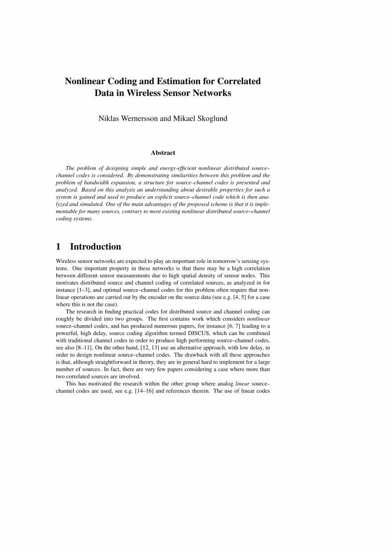
Nonlinear Coding and Estimation for CorrelatedData in Wireless Sensor Networks

Niklas Wernersson and Mikael Skoglund

Abstract

The problem of designing simple and energy-efficient nonlinear distributed source–channel codes is considered. By demonstrating similarities between this problem and theproblem of bandwidth expansion, a structure for source–channel codes is presented andanalyzed. Based on this analysis an understanding about desirable properties for such asystem is gained and used to produce an explicit source–channel code which is then ana-lyzed and simulated. One of the main advantages of the proposed scheme is that it is imple-mentable for many sources, contrary to most existing nonlinear distributed source–channelcoding systems.

1 IntroductionWireless sensor networks are expected to play an important role in tomorrow’s sensing sys-tems. One important property in these networks is that there may be a high correlationbetween different sensor measurements due to high spatial density of sensor nodes. Thismotivates distributed source and channel coding of correlated sources, as analyzed in forinstance [1–3], and optimal source–channel codes for this problem often require that non-linear operations are carried out by the encoder on the source data (see e.g. [4, 5] for a casewhere this is not the case).

The research in finding practical codes for distributed source and channel coding canroughly be divided into two groups. The first contains work which considers nonlinearsource–channel codes, and has produced numerous papers, for instance [6, 7] leading to apowerful, high delay, source coding algorithm termed DISCUS, which can be combinedwith traditional channel codes in order to produce high performing source–channel codes,see also [8–11]. On the other hand, [12, 13] use an alternative approach, with low delay, inorder to design nonlinear source–channel codes. The drawback with all these approachesis that, although straightforward in theory, they are in general hard to implement for a largenumber of sources. In fact, there are very few papers considering a case where more thantwo correlated sources are involved.

This has motivated the research within the other group where analog linear source–channel codes are used, see e.g. [14–16] and references therein. The use of linear codes

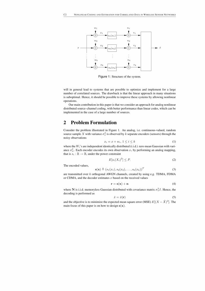
C2 NONLINEAR CODING AND ESTIMATION FOR CORRELATED DATA IN WIRELESS SENSOR NETWORKS

PSfrag replacements

......

......

s1(x1)

x

n1

n2

nk

x1

x2

xk

r1

w1

s2(x2)r2

w2

sk(xk)rk

wk

x

Figure 1: Structure of the system.

will in general lead to systems that are possible to optimize and implement for a largenumber of correlated sources. The drawback is that the linear approach in many situationsis suboptimal. Hence, it should be possible to improve these systems by allowing nonlinearoperations.

Our main contribution in this paper is that we consider an approach for analog nonlineardistributed source–channel coding, with better performance than linear codes, which can beimplemented in the case of a large number of sources.

2 Problem FormulationConsider the problem illustrated in Figure 1. An analog, i.e. continuous-valued, randomsource sample X with variance σ2

x is observed by k separate encoders (sensors) through thenoisy observations

xi = x + wi, 1 ≤ i ≤ k (1)

where the Wi’s are independent identically distributed (i.i.d.) zero mean Gaussian with vari-ance σ2

w . Each encoder encodes its own observation xi by performing an analog mapping,that is si : R → R, under the power constraint

E[si(Xi)2] ≤ P. (2)

The encoded values,s(x) , (s1(x1), s2(x2), . . . , sk(xk))T (3)

are transmitted over k orthogonal AWGN channels, created by using e.g. TDMA, FDMAor CDMA, and the decoder estimates x based on the received values

r = s(x) + n (4)

where N is i.i.d. memoryless Gaussian distributed with covariance matrix σ2nI . Hence, the

decoding is performed asx = x(r) (5)

and the objective is to minimize the expected mean square error (MSE) E[(X − X)2]. Themain focus of this paper is on how to design s(x).

3 DISCUSSION AND PROPOSED SCHEME C3

PSfrag replacements

s1(x)

s2(x)

n1 r1

s(x1)

s(x1)

n2

r2

s(x2)

s(x2)

Figure 2: x1 illustrates a ’small’ decoding error and x2 illustrates a ’large’ de-coding error.

3 Discussion and Proposed SchemeWe will in Subsections 3.A–B discuss two important special cases of the problem settingdescribed in Figure 1. Understanding for these special cases leads to insight about how todesign the encoding function s(x) for the general case. Based on this insight we presentand analyze a structure for s(x) in Subsections 3.C–D. Finally, based on the derived resultswe propose an explicit scheme for s(x) in Subsection 3.E.

3.1 σ2w > 0 and σ2

n → 0

For the case when σ2w > 0 and σ2

n → 0 the AWGN channels are approaching ideal,i.e. noiseless, channels and ri will approach si(xi). This means that given the linear en-coding strategy,

si(xi) = � P

σ2x + σ2

w

xi, 1 ≤ i ≤ k, (6)

the decoder will get access to the noisy observations {xi}ki=1 (since the channel is close to

perfect). Given these observations we could theoretically perform the best possible estima-tion based on the noisy observations as given by the Cramer–Rao lower bound, see e.g. [17].It is clear that there will be no way to obtain a better performance, since that would requirebetter sensor observations, and we can therefore conclude that the linear coding strategydescribed above is approaching the optimal strategy when σ2

n → 0.

3.2 σ2w = 0 and σ2

n > 0

In the case when σ2w = 0 and σ2

n > 0 we will get xi = x ∀i which we will write ass(x) = s(x). This problem is equivalent to the problem often referred to as the band-

C4 NONLINEAR CODING AND ESTIMATION FOR CORRELATED DATA IN WIRELESS SENSOR NETWORKS

width expansion problem mentioned already in one of Shannon’s first papers [18], seealso [19–21] and the references therein. It is well known for this problem that when thesource is i.i.d. zero-mean Gaussian and k = 1, linear encoding is optimal under the as-sumption that the decoder knows the source and noise variances. However, when k > 1this is no longer true and nonlinear encoding can have superior performance compared tolinear encoding strategies, see e.g. [22]. One of the reasons for this is that a linear encodingfunction s(x) uses only a one dimensional subspace of the available channel space. Moreefficient mappings would use a higher number of the available channel space dimensions.An example of this is illustrated in Figure 2 where k = 2 is assumed. By using nonlinearencoding functions, illustrated by the solid ’S–shaped’ curve s(x), we are able to better fillthe channel space than when using linear encoding functions, represented by the dashedcurve. A longer curve essentially means a higher resolution when estimating x as long aswe decode to the right fold of the curve, illustrated by sample x1 in the figure. However,decreasing the SNR will at some point result in that different folds of the curve will lie tooclose to each other and the decoder will start making large decoding errors, illustrated bysample x2 in the figure. Decreasing the SNR below this threshold will therefore signifi-cantly deteriorate the performance.

3.3 ObjectiveBased on the intuition from these two special cases we can conclude that for the problemconsidered in this paper, where both σ2

w > 0 and σ2n > 0, good encoding functions s(x)

should take both these aspects into consideration. We illustrate the use of a nonlinear en-coding function s(x) in Figure 3. Again, s(x) will be a point on the ’S–shaped’ curve.However, we are not encoding x but x which will create the point s(x). Hence, the distri-bution of points s(x) will be spread around the curve, as illustrated by the dotted region, and

PSfrag replacementss1(x)

s2(x)

s(x)

s(x)

s(x) n

r

Figure 3: Using a nonlinear encoding function s(x). The dotted region illus-trates the distribution of the encoded values s(x).

3 DISCUSSION AND PROPOSED SCHEME C5

the amount of spread will depend on the observation noise variance σ2w . When the encoded

value is transmitted over the channels we also get a noise contribution n from the channeland based on the received r the decoder creates the estimate x corresponding to some s(x).Our objective in this paper is to analyze and design nonlinear encoding functions s(x) ofthe type illustrated in Figure 3.

3.4 AnalysisIn order to gain understanding for the use of nonlinear encoding functions s(x) we makea performance analysis under the assumptions that σ2

w and σ2n are small. We also assume,

in this subsection, that all encoding functions si(xi) are continuous and differentiable andthat the curve s(x) is appropriately designed such that no large decoding errors occur underthe assumed noise variances.

Let us start by studying a certain encoded observation x and the resulting estimatex = x+z, with z representing the estimation error. Under the above assumptions, i.e. smallnoise variances, also z will be small and hence

s(x) = s(x + z) ≈ s(x) + zs′(x). (7)

where

s′(x) , � d

dxs1(x),

ddx

s2(x), . . . ,d

dxsk(x) T

. (8)

Now consider the decoder. It is well known that in order to minimize the MSE thedecoder should be implemented as

x(r) = E[X|r]. (9)

This function will however, in general, be difficult to implement. We will therefore considerthe suboptimal maximum likelihood (ML) decoder. Since σ2

w is small, s(x) can be linearlyapproximated as

s(x) ≈ s(x) + diag(s′(x))w (10)

which givesr = s(x) + n ≈ s(x) + diag(s′(x))w + n. (11)

We approximate1 the ML decoder as

x(r) = arg maxx

p(r|x) ≈ arg minx

‖s(x) − r‖2 (12)

where p(·|·) denotes the transition pdf from x to r. Hence, the decoding function corre-sponds to decoding r to the closest point on the curve s(x). However, for small values of|x − x| the curve s(x) is approximately linear and parallel to s′(x). This means that thedecoder will remove the noise contributions orthogonal to s′(x) and we get

s(x) ≈ s(x) +(diag(s′(x))w + n) · s′(x)

‖s′(x)‖s′(x)

‖s′(x)‖ (13)

1The true ML decoder will be difficult to analyze since the variances of the resulting noise terms in(11) will depend on x.

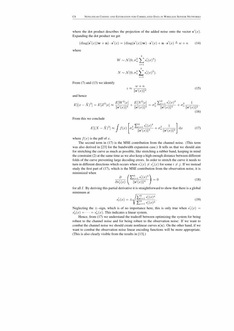
C6 NONLINEAR CODING AND ESTIMATION FOR CORRELATED DATA IN WIRELESS SENSOR NETWORKS

where the dot product describes the projection of the added noise onto the vector s′(x).Expanding the dot product we get

(diag(s′(x))w + n) · s′(x) = (diag(s′(x))w) · s′(x) + n · s′(x) , w + n (14)

where

W ∼ N (0, σ2w

k�i=1

s′i(x)4)

N ∼ N (0, σ2n

k�i=1

s′i(x)2).

From (7) and (13) we identify

z ≈ w + n

‖s′(x)‖2(15)

and hence

E[(x − X)2] = E[Z2|x] ≈ E[W 2|x]

‖s′(x)‖4+

E[N2|x]

‖s′(x)‖4= σ2

w � k

i=1 s′i(x)4

‖s′(x)‖4+ σ2

n

1

‖s′(x)‖2.

(16)

From this we conclude

E[(X − X)2] ≈�

f(x) � σ2w � k

i=1 s′i(x)4

‖s′(x)‖4+ σ2

n

1

‖s′(x)‖2 � dx (17)

where f(x) is the pdf of x.The second term in (17) is the MSE contribution from the channel noise. (This term

was also derived in [23] for the bandwidth expansion case.) It tells us that we should aimfor stretching the curve as much as possible, like stretching a rubber band, keeping in mindthe constraint (2) at the same time as we also keep a high enough distance between differentfolds of the curve preventing large decoding errors. In order to stretch the curve it needs toturn in different directions which occurs when s′i(x) 6= s′j(x) for some i 6= j. If we insteadstudy the first part of (17), which is the MSE contribution from the observation noise, it isminimized when

∂

∂s′I(x) � � k

i=1 s′i(x)4

‖s′(x)‖4 � = 0 (18)

for all I . By deriving this partial derivative it is straightforward to show that there is a globalminimum at

s′I(x) = ± � � k

i=1 s′i(x)4� k

i=1 s′i(x)2. (19)

Neglecting the ±–sign, which is of no importance here, this is only true when s′1(x) =s′2(x) = · · · = s′k(x). This indicates a linear system.

Hence, from (17) we understand the tradeoff between optimizing the system for beingrobust to the channel noise and for being robust to the observation noise: If we want tocombat the channel noise we should create nonlinear curves s(x). On the other hand, if wewant to combat the observation noise linear encoding functions will be more appropriate.(This is also clearly visible from the results in [13].)

3 DISCUSSION AND PROPOSED SCHEME C7

3.5 Proposed SchemeBased on the analysis in Section 3.4 we concluded that linear functions s(x) are good withrespect to the observation noise but inefficient with respect to the channel noise. Therefore,in order to produce a system which is able to handle both observation and channel noise,we propose a piecewise linear encoding function s(x) as follows

si(xi) = � αxi 1 ≤ i ≤ k0

α(xi − ∆ xi

∆ ! ) k0 < i ≤ k(20)

where b·e denotes rounding to the nearest integer and α will control the power usage.Hence, we allow noncontinuous and nondifferentiable functions which was not the casein the analysis. The reason is that this results in a system where s′1(x) = s′2(x) = · · · =s′k(x), except at the discontinuities, which is desirable with respect to the observation noise.At the same time we get a nonlinear system, better able to use the available channel space,which is desirable with respect to the channel noise. The drawback is that the approximationin (11) is violated making the decoder (12) inefficient. We therefore modify the decodingfunction as follows:

1. Create the ML estimate of x based on the linear encoding functions:

xk0 =1

k0

k0�i=1

ri

α. (21)

2. Assume that |xk0 −xi −ni/α| ≤ ∆/2 for k0 < i ≤ k and create the ML estimates

xi(ri) = arg minxi " (si(xi) − ri)

2|xi ∈ {|xk0 − xi| ≤ ∆/2} # . (22)

This function tries to predict the removed part ∆ xi

∆ ! from (20) based on the derivedxk0 . The operation is illustrated in in Figure 4 for a few examples.

3. Based on this, create the final estimate of x as

x =1

k �� k0�i=1

ri

α+

k�i=k0+1

xi(ri) �� . (23)

Let us now analyze the power consumption. Note that the power used by the nonlinearencoding functions will be less than the power used by the linear encoding functions. Wedefine the normalized average power consumption as

P (∆, k0) =1

kα2 " k0E[sI(XI)2] + (k − k0)E[sJ(XJ)2] # (24)

where we assume I ≤ k0 < J ≤ k. (The reason for dividing with α2 is that we wantP (∆, k0) to represent the change in power consumption due to ∆ and k0 and not due tothe scaling factor α.) By performing timesharing the sensors could use the linear encodingfunction for a fraction k0/k of the available time slots and then use the nonlinear encodingfunctions the rest of the time. Hence, P (∆, k0) can be seen as the average power used byeach sensor when α = 1.

C8 NONLINEAR CODING AND ESTIMATION FOR CORRELATED DATA IN WIRELESS SENSOR NETWORKS

PSfrag replacements

n1

x1 x1

si(x)

x

n2

n3

xk0x3 x2x2x2

Figure 4: Illustration of the decoding function for the nonlinear encoding func-tion si(x). The decoder assumes that |xk0 − xi − ni/α| ≤ ∆/2 andtherefore limits the estimate xi to lie within this interval, illustratedwith the white area in the figure. Three examples are shown, for x1

the assumption made is correct and the estimation of the nonlinearpart ∆ xi

∆ ! is correct. For x2 the assumption made is incorrect andthe estimated nonlinear part will be wrong. Finally, for x3 the as-sumption is actually wrong but the estimated nonlinear part will stillbe decoded correctly resulting in x3 = x3.

4 Performance Analysis

It is clear that the performance of the system proposed in (20), given a certain P , willdepend on ∆ and k0. In order to optimize these parameters we will here derive the MSE asa function of ∆ and k0 under the assumption that x is i.i.d. zero–mean Gaussian. Hence,evaluating this function for different choices of ∆ and k0 will provide a possibility to designthe system for a certain set of noise variances.

For a given ∆ and k0 we should choose

α = � P

P (∆, k0)(25)

in order to get the power consumption P . In order to simplify the following equations wewill instead study the equivalent system where α = 1 and the channel noise variance equalsP (∆, k0)/Pσ2

n.

4 PERFORMANCE ANALYSIS C9

Given a certain r and x the decoder in (23) will produce

x(r,x) ≈ 1

k

k�i=1

(xi + ni)$ %�& ',xa

+

k�i=k0+1

∆

k ( xk0 − xi − ni

∆ )$ %*& ',xb

(26)

where xb is a penalty term arising if |xk0 − xi − ni| > ∆/2 meaning that the assumptionmade in (22) is incorrect. This situation is illustrated with sample x2 in Figure 4. Thereason for using an approximation sign in (26) is the kind of situation illustrated by samplex3 in Figure 4. For this example |xk0 −xi −ni| > ∆/2 is true but the estimated nonlinearpart is still correct. Hence, in some specific cases the decoder (23) will perform better thanwhat is described by (26).

For the expected MSE we get

MSE(∆, k0) = E[(X − X)2] = E[(X − Xa − Xb)2]

= E[(X − Xa)2] + E[(Xb)2] + 2E[(X − Xa)Xb] (27)

where we directly see

E[(X − Xa)2] =σ2

w + P (∆, k0)/Pσ2n

k. (28)

Here we see the role played by ∆ and k0: decreasing ∆ and/or k0 will decrease P (∆, k0)and hence lower the effective channel noise variance. At the same time we can expect thesecond term in (27) to increase since the assumption made in (22) will get more likely to beincorrect. For the second term we get

E[X2b ] = (k − k0)

∆2

k2 � E �,+ Xk0 − Xi − Ni

∆ - 2 �+(k − k0 − 1)E �.+ Xk0 − Xi − Ni

∆ - + Xk0 − Xj − Nj

∆ - �/�= (k − k0)

∆2

k2 � E � ( ξi

∆ ) 2 � + (k − k0 − 1)E 0 ( ξi

∆ )1( ξj

∆ ).2 � (29)

where i 6= j, ξi , Xk0 − Xi − Ni and

Xk0 − Xi − Ni ∼ N (0, (1

k0+ 1)(σ2

w + P (∆, k0)/Pσ2n)). (30)

It is straightforward to calculate the first expected value in (29) by using the Q-function. Forthe second expected value we need to consider that the resulting Gaussian terms ξi and ξj

are correlated since they both contain xk0 . The expression can be evaluated numerically orotherwise well approximated by approximating the jointly Gaussian distribution f(ξi, ξj)as a Gaussian Mixture

f(ξi, ξj) ≈ 1

4πσ2e−

(ξ1−µ)2

2σ2 e−

(ξ2−µ)2

2σ2 +1

4πσ2e−

(ξ1+µ)2

2σ2 e−

(ξ2+µ)2

2σ2 (31)

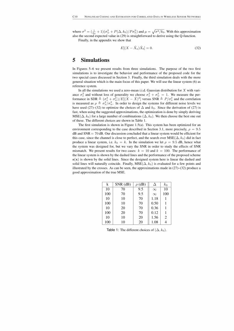
C10 NONLINEAR CODING AND ESTIMATION FOR CORRELATED DATA IN WIRELESS SENSOR NETWORKS

where σ2 = ( 1k0

+ 1)(σ2w + P (∆, k0)/Pσ2

n) and µ = � σ2/k0. With this approximationalso the second expected value in (29) is straightforward to derive using the Q-function.

Finally, in the appendix we show that

E[(X − Xa)Xb] = 0. (32)

5 SimulationsIn Figures 5–6 we present results from three simulations. The purpose of the two firstsimulations is to investigate the behavior and performance of the proposed code for thetwo special cases discussed in Section 3. Finally, the third simulation deals with the moregeneral situation which is the main focus of this paper. We will use the linear system (6) asreference system.

In all the simulations we used a zero-mean i.i.d. Gaussian distribution for X with vari-ance σ2

x and without loss of generality we choose σ2x + σ2

w = 1. We measure the per-formance in SDR , (σ2

x + σ2w)/E[(X − X)2] versus SNR , P/σ2

n and the correlationis measured as ρ , σ2

x/σ2w . In order to design the systems for different noise levels we

have used (27)–(32) to optimize the choices of ∆ and k0. Since the derivation of (27) isfast, when using the suggested approximations, the optimization is done by simply derivingMSE(∆, k0) for a large number of combinations (∆, k0). We then choose the best one outof these. The different choices are shown in Table 1.

The first simulation is shown in Figure 1.5(a). This system has been optimized for anenvironment corresponding to the case described in Section 3.1, more precisely, ρ = 9.5dB and SNR = 70 dB. Our discussion concluded that a linear system would be efficient forthis case, since the channel is close to perfect, and the search over MSE(∆, k0) did in factproduce a linear system, i.e. k0 = k. In the simulation we let ρ = 9.5 dB, hence whatthe system was designed for, but we vary the SNR in order to study the effects of SNRmismatch. We present results for two cases: k = 10 and k = 100. The performance ofthe linear system is shown by the dashed lines and the performance of the proposed schemes(x) is shown by the solid lines. Since the designed system here is linear the dashed andsolid lines will naturally coincide. Finally, MSE(∆, k0) is evaluated for a few points andillustrated by the crosses. As can be seen, the approximations made in (27)–(32) produce agood approximation of the true MSE.

k SNR (dB) ρ (dB) ∆ k0

10 70 9.5 ∞ 10100 70 9.5 ∞ 10010 10 70 1.18 1

100 10 70 0.50 110 20 70 0.36 1

100 20 70 0.12 110 10 20 1.56 2

100 10 20 1.08 4

Table 1: The different choices of (∆, k0).

5 SIMULATIONS C11

0 5 10 15 20 25 305

10

15

20

25

30

35

Linear

PSfrag replacements

s(x)

k = 100

k = 10

SNR (dB)

SDR

(dB

)

(a)

0 5 10 15 20 25 300

10

20

30

40

50

60

70

Linear

PSfrag replacements

s(x)

k = 100

k = 10

SNR (dB)

SDR

(dB

)

(b)

0 5 10 15 20 25 305

10

15

20

25

30

35

40

Linear

PSfrag replacements

s(x)

k = 100

k = 10

SNR (dB)

SDR

(dB

)

(c)

Figure 5: Systems for k = 10 and k = 100 designed for (a) ρ = 9.5dB andSNR= 70dB (b) ρ = 70dB and SNR= 10dB as well as SNR= 20dB(c) ρ = 20 dB and SNR= 10dB. In all simulations the ’true’ ρ hasbeen used but the SNR is varied.

C12 NONLINEAR CODING AND ESTIMATION FOR CORRELATED DATA IN WIRELESS SENSOR NETWORKS

0 5 10 15 20 25 30 35 40 45 505

10

15

20

25

30

35

40

Linear

PSfrag replacements

s(x)

k = 100

k = 10

ρ (dB)

SDR

(dB

)

(a)

Figure 6: Systems for k = 10 and k = 100 designed for ρ = 20 dB andSNR= 10dB. In both simulations the ’true’ SNR has been used butthe ρ is varied.

In Figure 1.5(b) the systems have been optimized for an environment corresponding tothe case described in Section 3.2, i.e. close to bandwidth expansion which occurs when ρhas a high value. We have here included two designs for ρ = 70 dB, namely SNR = 10 dBand SNR = 20 dB. Hence, one of the systems is optimized for a better channel meaningthat different folds of s(x) should be packed closer to each other. This will give a betterperformance for high SNR’s but the code will also break down faster when the SNR isdecreased. This is clearly visible in the figure where we again simulate for the designedρ but vary the SNR. The linear systems represented by the dashed curves are the bettersystems only for low SNR’s.

Finally, we consider the, for this paper, most interesting case where we optimize asystem for both observation and channel noise. In Figure 1.5(c) we have designed systemsfor ρ = 20 dB and SNR = 10 dB. Also here we simulate for the designed ρ but we vary theSNR. It is clear that there will be a large gain over the linear system except at low SNR’s,where the source–channel code breaks down, and at high SNR’s, where there is no gain inusing nonlinear codes. In Figure 6 we instead evaluate the effects of correlation mismatchfor the same system. That is, we evaluate the performance of the same system as above butthis time we simulate for the designed SNR and let ρ vary. As can be seen the system is quitesensitive to a too low ρ whereas a higher ρ only gives a slight improvement in performance.

6 ConclusionsWe have explained the similarities between the problem of distributed source–channel cod-ing and the problem of bandwidth expansion. Based on this we have presented and analyzeda suitable structure for distributed source–channel codes. This analysis gives us insight intodesirable properties for such a system. Based on this understanding an explicit code is pre-sented, analyzed and simulated. The code is implementable for many sources, contrary to

6 CONCLUSIONS C13

most existing schemes, and it is concluded that a large gain is obtained from the nonlinearcode compared to the linear code.

AppendixWe will here show that the third term in (27) equals 0. When doing so we will use thevariable

Ui = Wi + Ni

with pdf f(ui) and variance σ2u = σ2

w + P (∆, k0)/Pσ2n. Since both Wi and Ni are

i.i.d. Gaussian also Ui will naturally be i.i.d. Gaussian. We will also use the variables I andJ such that I ≤ k0 < J . We get

E[(X − Xa)Xb] = E �� � X − 1

k

k�i=1

(Xi + Ni) � �� k�j=k0+1

∆

k+ Xk0 − Xj − Nj

∆ - �� ��=

∆

k2E �� � k�

i=1

Ui � �� k�j=k0+1

+ 1k0 � k0

i=1 Ui − Uj

∆ - �� ��=

∆(k − k0)

k2E � � k�

i=1

Ui � + 1k0 � k0

i=1 Ui − UJ

∆ - �=

∆(k − k0)

k2 � k0E � UI + 1k0 � k0

i=1 Ui − UJ

∆ - � +

E � UJ + 1k0 � k0

i=1 Ui − UJ

∆ - �/�=

∆(k − k0)

k2 � k0E � UI + UI

k0+ ξ1

∆ - � − E 0 UJ ( UJ + ξ2

∆ ),2 �(33)

where

ξ1 ∼ N � 0, � k0 − 1

k20

+ 1 σ2u

ξ2 ∼ N � 0,1

k0σ2

u .

Studying the first resulting expected value in (33), with the expectation taken over UI , weget

E � UI + UI

k0+ ξ1

∆ - � =

∞�i=−∞

i

� k0(i∆+ ∆2−ξ1)

k0(i∆−∆2−ξ1)

uIf(uI)duI

= � σ2u

2π

k=∞�k=−∞

e−

k20(i∆−

∆2

−ξ1)2

2σ2u . (34)

C14 ON SOURCE DECODING BASED ON FINITE-BANDWIDTH SOFT INFORMATION

The second expected value in (33) can be derived in the same manner and produces a similarresult. This gives

E[(X − Xa)Xb] =∆(k − k0)

k2� σ2

u

2π

∞�i=−∞

E � k0e−

k20(i∆−

∆2

−ξ1)2

2σ2u − e

−(i∆−

∆2

−ξ2)2

2σ2u �

(35)where the expectation is on ξ1 and ξ2. Straightforward derivations, for a general case cov-ering both the expected values in (35), gives

E 3 e−γ(β−ξ)2 4 =

� ∞−∞

1� 2πσ2ξ

e(−γ(β−ξ)2)e− ξ2

2σ2ξ dξ =

e− γβ2

2γσ2ξ+1� 2γσ2

ξ + 1(36)

and by substituting γ, β and σ2ξ with the corresponding coefficients from (35), followed by

a few manipulations, it turns out that

E � k0e−

k20(i∆−

∆2

−ξ1)2

2σ2u � = E � e− (i∆−

∆2

−ξ2)2

2σ2u � . (37)

Therefore, we can conclude, from (35), that

E[(X − Xa)Xb] = 0. (38)

References[1] D. Slepian and J. Wolf, “Noiseless coding of correlated information sources,” IEEE

Transactions on Information Theory, vol. 19, no. 4, pp. 471–480, July 1973.

[2] A. D. Wyner and J. Ziv, “The rate-distortion function for source coding with sideinformation at the decoder,” IEEE Transactions on Information Theory, vol. IT-22,no. 1, pp. 1–10, January 1976.

[3] J. J. Xiao and Z. Q. Luo, “Multiterminal source-channel communication over an or-thogonal multiple-access channel,” IEEE Transactions on Information Theory, vol. 53,no. 9, pp. 3255–3264, September 2007.

[4] M. Gastpar and M. Vetterli, “Source-channel communication in sensor networks,” inProc. 2nd Int. Workshop Information Processing in Sensor Networks (IPSN03) (Lec-ture Notes in Computer Science), L. J. Guibas and F. Zhao, Eds. Berlin, Germany:Springer-Verlag, 2003, pp. 162–177.

[5] M. Gastpar, “Uncoded transmission is exactly optimal for a simple gaussian ”sensor”network,” in Proc. 2nd Annu. Workshop on Information Theory and its Applications,,January 2007, pp. 177–182.

[6] A. Wyner, “Recent results in the shannon theory,” IEEE Transactions on InformationTheory, vol. 20, no. 1, pp. 2–10, January 1974.

REFERENCES C15

[7] S. S. Pradhan and K. Ramchandran, “Distributed source coding using syndromes(DISCUS): design and construction,” IEEE Transactions on Information Theory,vol. 49, no. 3, pp. 626–643, March 2003.

[8] A. D. Liveris, Z. Xiong, and C. N. Georghiades, “Compression of binary sources withside information at the decoder using LDPC codes,” IEEE Communications Letters,vol. 6, no. 10, pp. 440–442, October 2002.

[9] J. Garcia-Frias and Y. Zhao, “Compression of correlated binary sources using turbocodes,” IEEE Commnications Letters, vol. 5, no. 10, pp. 417–419, October 2001.

[10] Z. Xiong, A. Liveris, S. Cheng, and Z. Liu, “Nested quantization and Slepian-Wolfcoding: a Wyner-Ziv coding paradigm for i.i.d. sources,” in IEEE Workshop on Sta-tistical Signal Processing, September 2003, pp. 399–402.

[11] S. Pradhan and K. Ramchandran, “Generalized coset codes for distributed binning,”IEEE Transactions on Information Theory, vol. 51, no. 10, pp. 3457–3474, October2005.

[12] A. Saxena and K. Rose, “Distributed predictive coding for spatio-temporally corre-lated sources,” in Proceedings IEEE Int. Symp. Information Theory, June 2007, pp.1506–1510.

[13] N. Wernersson, J. Karlsson, and M. Skoglund, “Distributed quantization over noisychannels,” IEEE Transactions on Communications, 2008, to appear.

[14] Z. Luo, G. Giannakis, and S. Zhang, “Optimal linear decentralized estimation in abandwidth constrained sensor network,” in Proceedings IEEE Int. Symp. InformationTheory, September 2005, pp. 1441–1445.

[15] I. Bahceci and A. K. Khandani, “Energy-efficient estimation of correlated data in wire-less sensor networks,” in Annual Conference on Information Sciences and Systems,March 2006, pp. 973–978.

[16] S. Cui, J. Xiao, A. Goldsmith, Z. Luo, and V. Poor, “Estimation diversity and energyefficiency in distributed sensing,” IEEE Transactions on Signal Processing, vol. 55,no. 9, pp. 4683–4695, September 2007.

[17] S. M. Kay, Fundamentals of Statistical Signal Processing: Estimation Theory. Pren-tice Hall, 1993.

[18] C. E. Shannon, “Communication in the presence of noise,” Proc. IRE, pp. 10–21,January 1949.

[19] B. Chen and G. W. Wornell, “Analog error-correcting codes based on chaotic dynam-ical systems,” IEEE Transactions on Communications, vol. 46, no. 7, pp. 881–890,July 1998.

[20] V. Vaishampayan and S. I. R. Costa, “Curves on a sphere, shift-map dynamics, and er-ror control for continuous alphabet sources,” IEEE Transactions on Information The-ory, vol. 49, no. 7, pp. 1658–1672, July 2003.

[21] N. Wernersson, M. Skoglund, and T. Ramstad, “Analog source-channel codes basedon orthogonal polynomials,” in Asilomar Conference on Signals, Systems and Com-puters, November 2007.

[22] J. M. Wozencraft and I. M. Jacobs, Principles of Communication Engineering. Wiley,1965.

[23] D. J. Sakrison, Transmission of Waveforms and Digital Information. Wiley, 1968.

Paper D

Sorting–Based Multiple Description Quantization

Niklas Wernersson and Mikael SkoglundPublished in IEEE Transactions of Communications, 2006

c©2006 IEEEThe layout has been revised

Sorting–Based Multiple Description Quantization

Niklas Wernersson and Mikael Skoglund

Abstract

We introduce a new method for multiple description quantization (MDQ), based onsorting a frame of samples and transmitting, as side-information/redundancy, an index thatdescribes the resulting permutation. The sorting-based approach has a similar performanceto multiple description scalar quantization and a flexible structure, providing straightfor-ward implementation of multi-dimensional MDQ.

1 IntroductionPacket networks have gained in importance in recent years, for instance by the wide-spreaduse and importance of the Internet. Unfortunately, packet losses in these systems can ingeneral not be neglected and this has to be taken into account in robust source–channelcoding for multimedia communications. One way to deal with packet losses is to use mul-tiple description coding/quantization where the objective is to code one source of data intomultiple bitstreams. The coding is done in such a way that multiple levels of quality isachieved. This means that even if one or a few of the bitstreams are lost, the received bitsshould make it possible to get an approximated version of the original data. MDQ willtherefore enhance the reliability of the communication system. Multiple-description codinghas received considerable attention, see e.g. [1–5].

In this letter we present an MDQ method which uses sorting in the transmitter in orderto produce a low-quality description of a source frame. This description, if received, canbe used in the receiver either to produce a low-quality estimate or otherwise to improve anexisting estimate based on other descriptions.

The letter is organized as follows. In Section 2 sorting-based MDQ is introduced. InSection 3 a basic analysis of the the new method is presented. Finally, we provide numericalresults and conclusions in Sections 4–5.

2 Sorting-Based MDQThe proposed method is illustrated in Figure 1. Consider independent identically distributed(i.i.d) random variables X1, X2, . . . , XM , Xi ∈ R, with probability density function p(x)of support [L, U ], −∞ ≤ L < U ≤ ∞. These variables are to be quantized and transmitted

D2 SORTING–BASED MULTIPLE DESCRIPTION QUANTIZATION

PSfrag replacements

X1 X1

X2X2

XM XM

j1

j2

jM

I

I

...

...

...

...

......

...Q

Q

Q Channel 1

Channel 2

Channel M

Channel M + 1

Channel M + r

X1

X2

XM

Sort

Figure 1: Sorting-based MDQ. A frame of random source samples are sortedin the transmitter. Quantized versions of these observations are thentransmitted over different channels, as well as the index I containinginformation about how the observations were sorted. The receivedinformation is then used to estimate the original observations.

over a network using M + r packets. We assume that the transmitted packets will beindependently lost during the transmission meaning that it may be necessary to reconstructthe original data from only a subset of the transmitted packets. The suggested approachis then based on sorting1 the observed random variables in the transmitter. The sortingprocedure will rearrange a copy of the original values in ascending order. With IM ={1, . . . , M}, let π : IM → IM describe the corresponding permutation of the indices1, 2, . . . , M such that

Xπ(1) ≤ Xπ(2) ≤ · · · ≤ Xπ(M). (1)

That is, π(1) denotes the original index of the smallest Xi, etc. There are M ! possiblepermutations. Let I ∈ {1, . . . , M !} be an integer that uniquely describes π, see e.g. [6] fordetails on how to determine such an index based on π. The index I can be represented inbinary form using

f(M) & log2(M !) (2)

bits (with “ & ” meaning “close to from above”). After sorting, X1, X2, .., XM are quan-tized using M identical memoryless scalar quantizers. Letting Rj = [lj , uj), L ≤ lj <uj ≤ U , denote the jth quantization region, the encoding produces the indices j1, . . . , jM

as Xi ∈ Rj ⇒ ji = j. These indices are then transmitted over M channels together withr identical copies of the index I , using r additional channels.

Let Xi be the reconstructed version of Xi. In this letter we assume that the mean–square error (MSE), E[(Xi − Xi)

2], is used as a distortion measure. We will also as-sume that the different channels independently lose descriptors (packets) with probabilityp. Hence, due to the imperfections in the network some of the transmitted descriptors maybe lost which leads to essentially four different cases when computing Xπ(i):

1There are numerous sorting algorithms in the literature which can be used in the transmitter, forinstance Heap sort, having an O(M log M) complexity which, for our application, is tolerable.

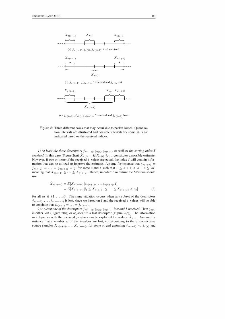
2 SORTING-BASED MDQ D3

PSfrag replacementsXπ(i−1) Xπ(i) Xπ(i+1)

(a) jπ(i−1), jπ(i), jπ(i+1), I all received.

PSfrag replacements

Xπ(i−1) Xπ(i+1)

Xπ(i)

(b) jπ(i−1), jπ(i+1), I received and jπ(i) lost.

PSfrag replacements Xπ(i−2) Xπ(i) Xπ(i+1)

Xπ(i−1)

(c) jπ(i−2), jπ(i), jπ(i+1), I received and jπ(i−1) lost.

Figure 2: Three different cases that may occur due to packet losses. Quantiza-tion intervals are illustrated and possible intervals for some Xi’s areindicated based on the received indices.

1) At least the three descriptors jπ(i−1), jπ(i), jπ(i+1) as well as the sorting index I

received. In this case (Figure 2(a)) Xπ(i) = E[Xπ(i)|jπ(i)] constitutes a possible estimate.However, if two or more of the received j–values are equal, the index I will contain infor-mation that can be utilized to improve the estimate. Assume for instance that jπ(s+1) =jπ(s+2) = . . . = jπ(s+z) = j, for some s and z such that 1 ≤ s + 1 < s + z ≤ M ,meaning that Xπ(s+1) ≤ · · · ≤ Xπ(s+z). Hence, in order to minimize the MSE we shoulduse

Xπ(s+m) = E[Xπ(s+m)|jπ(s+1), . . . , jπ(s+z), I]

= E[Xπ(s+m)|lj ≤ Xπ(s+1) ≤ · · · ≤ Xπ(s+z) < uj ] (3)

for all m ∈ {1, . . . , z}. The same situation occurs when any subset of the descriptorsjπ(s+2), . . . , jπ(s+z−1) is lost, since we based on I and the received j–values will be ableto conclude that jπ(s+1) = . . . = jπ(s+z).

2) At least one of the descriptors jπ(i−1), jπ(i), jπ(i+1) lost and I received. Here jπ(i)

is either lost (Figure 2(b)) or adjacent to a lost descriptor (Figure 2(c)). The informationin I together with the received j–values can be exploited to produce Xπ(i). Assume forinstance that a number w of the j–values are lost, corresponding to the w consecutivesource samples Xπ(s+1), . . . , Xπ(s+w), for some s, and assuming jπ(s−1) < jπ(s) and

D4 SORTING–BASED MULTIPLE DESCRIPTION QUANTIZATION

jπ(s+w+1) < jπ(s+w+2), for simplicity. The estimate Xπ(s+m) can then be computed as

Xπ(s+m) =E[Xπ(s+m)|jπ(s), jπ(s+w+1), I]

=E[Xπ(s+m)|ljπ(s)≤ Xπ(s) ≤ Xπ(s+1) ≤ · · ·

· · · ≤ Xπ(s+w) ≤ Xπ(s+w+1) < ujπ(s+w+1),

ljπ(s)≤ Xπ(s) < ujπ(s)

, ljπ(s+w+1)≤ Xπ(s+w+1) < ujπ(s+w+1)

] (4)

for m = 0, . . . , w + 1. Note that this formula is used also for m = 0 and m = w + 1corresponding to received j–values. However, three special cases have to be considered,leading to modifications. These occur when s + 1 = 1 and/or s + w = M meaning that nolower/upper bound of the lost sequence is received, in which case we need to use L and/orU to bound the sequence. If s + 1 = 1 we get

Xπ(m) = E[Xπ(m)|L ≤ Xπ(1) ≤ · · · ≤ Xπ(w) ≤ Xπ(w+1) < ujπ(w+1),

ljπ(w+1)≤ Xπ(w+1) < ujπ(w+1)

] (5)

for m = 1, . . . , w + 1. Similarly, if s + w = M

Xπ(s+m) = E[Xπ(s+m)|ljπ(s)≤ Xπ(s) ≤ · · · ≤ Xπ(M) ≤ U, ljπ(s)

≤ Xπ(s) < ujπ(s)]

(6)

for m = 0, . . . , w. If both cases occur simultaneously we will get a similar formula to (3),where the source data are bounded by L and U and the index I alone will give a descriptionof the sequence {Xi}M

i=1.3) The descriptor ji received and I lost. Here no additional information about Xi is

received, so we useXi = E[Xi|ji]. (7)

4) Both ji and I lost. In this case we do not receive any information at all about Xi,hence we use

Xi = E[Xi]. (8)

We note here that the structure proposed in Figure 1 transmits r identical copies of I ,while better performance can actually be obtained for r > 1 if the coordinate system of thesource data is rotated before producing each copy of I , resulting in I1 6= I2 6= . . . 6= Ir .These indices, if received, can be used jointly to produce a better descriptor. In this letter,designing such rotations is however left as a topic for future work.

3 AnalysisHere we will further analyze the reconstruction formulas (3)–(4), under the assumptionthat Xi is uniformly distributed on [L, U ] = [0, 1]. We start by expanding (3) assuminga number z of the X–values are quantized to the same quantization cell, with index j. Auniform distribution gives

Xπ(s+m) = E[Xπ(s+m)|lj ≤ Xπ(s+1) ≤ · · · ≤ Xπ(s+z) < uj ] = lj +m

z + 1(uj − lj)

(9)

4 NUMERICAL RESULTS D5

for all m ∈ {1, . . . , z}, stating the quite intuitive result that the reconstruction points shouldbe spread out with an equal distance on the interval bounded by the jth quantization region.For the expression (4) we get

Xπ(s+m) = E[Xπ(s+m)|jπ(s), jπ(s+w+1), I] = ljπ(s)+

K(m + 1)(1 − (1 − u)w+3 − lw+3 + (l − u)w+3)

1 − (1 − u)(w+2) − l(w+2) + (l − u)(w+2)+

Ku(w + 3)((l − u)(w+2) − (1 − u)(w+2))

1 − (1 − u)(w+2) − l(w+2) + (l − u)(w+2),

where K =ujπ(s+w+1)

− ljπ(s)

w + 3, u =

ujπ(s)− ljπ(s)

ujπ(s+w+1)− ljπ(s)

, l =ljπ(s+w+1)

− ljπ(s)

ujπ(s+w+1)− ljπ(s)

(10)

for m = 0, . . . , w + 1, assuming w consecutive descriptors have been lost. In a similarmanner we get

Xπ(m) = E[Xπ(m)|jπ(w+1), I]

=(ujπ(w+1)

)

w + 2

m(1 − (ljπ(w+1)/ujπ(w+1)

)w+2)

1 − (ljπ(w+1)/ujπ(w+1)

)w+1, for m = 1, . . . , w + 1

(11)

Xπ(s+m) = E[Xπ(s+m)|jπ(s), I]

= ljπ(s)+

(1 − ljπ(s))

w + 2

(m + 1)(1 − (1 − u)w+2) − u(w + 2)(1 − u)w+1

1 − (1 − u)w+1

where u =ujπ(s)

− ljπ(s)

1 − ljπ(s)

for m = 0, . . . , w (12)

from (5) and (6), corresponding to the cases when we do not receive any descriptors pro-ducing a lower/upper limit for the lost sequence.

We also introduce a restriction on the rate RX that can be used per quantizer. Let Rdenote the total rate per symbol Xi. In the case M = 1 and no sorting index, we wouldget RX = R. However, increasing M and transmitting the sorting index will cost an extraf(M), from (2), bits per M source samples. Hence, fixing the total rate per transmittedsymbol we require the quantizers to restrict their rate to

RX = R − M−1 f(M). (13)

From (2)–(13) a closed-form analytical expression for the MSE when using sorting-based MDQ for a uniform source distribution can be derived, as shown in the appendix.The MSE will depend on 4 parameters, namely r – the retransmission index, M – the framesize, p – the packet loss probability and finally R – the rate per symbol. Using this formula,assuming R fixed and p known, we can optimize the choice of (M, r).

4 Numerical ResultsWe investigate the performance of sorting-based MDQ for i.i.d uniform Xi’s by compar-ing to two other methods: 1) A scheme based on forward error correction (FEC) using

D6 SORTING–BASED MULTIPLE DESCRIPTION QUANTIZATION

0 0.05 0.1 0.15 0.2 0.25 0.3 0.35 0.40

5

10

15

20

25

30

35

40

45

50Index safeMDSMDSQSortingUncoded

0 0.005 0.01 0.015 0.0210

20

30

40

50

PSfrag replacements

p

SDR

(dB

)Figure 3: We compare sorting-based MDQ (solid line), MDS coding

(dashed/dot), MDSQ (dashed) and an uncoded system (small dots).The circles show simulated results of a sorting-based MDQ system,coinciding with the analytical curve. We also illustrate the perfor-mance of sorting-based MDQ when the sorting index is transmittedover an error–free channel (larger dots). The systems are optimizedfor R = 8 and p = 0.002 (giving (M, r) = (7, 1) for sorting–basedMDQ).

maximum distance separable (MDS) codes [7] (MDS codes have the maximum possibleminimum distance between codewords). In order to make the comparison fair we requiredthe FEC to produce M + r descriptors when encoding k Xi’s, that is M + r channels areused. Such an MDS code will be able to correct M + r−k losses. Reference [8] presents aformula to calculate an approximate value of the MSE when a given number of descriptorsare lost, in a system with scalar quantization and FEC based on an MDS code. This ap-plies directly to our setup, and can easily be extended to give an analytical MSE for a givenpacket loss probability, p; 2) We also compare to a practical MDQ system, namely multipledescription scalar quantization (MDSQ) [1]. This method will use fewer channels than theproposed method but on the other hand it has a higher design complexity. In Figures 3–4 thedifferent systems are compared when optimized 2 for different loss probabilities and R = 8.In Figure 3 the systems are optimized for p = 0.002 and in Figure 4 for p = 0.01. Per-formance is studied by plotting the signal-to-distortion ratio (SDR), E[X2]/E[(X − X)2],versus p. Magnified versions of the plots are also included to show the region with low lossprobability in more detail. The solid line shows the performance of sorting-based MDQbased on the analytical formula (14) presented in the appendix. The circles are from a sim-

2For the MDS code the best k is found. For sorting-based MDQ (14) is minimized. However,since MDSQ is specified by the two design parameters n ∈ {0, . . . , 2

R2 − 1} and λ ∈ R

+, thereare an infinite number of possible systems. We designed all possible combinations of n and λ ∈{0, 0.001, 0.01, 0.1, 1, 10, 100, 1000} corresponding to a wide range of systems with no protectionto high protection. The best of these was chosen.

4 NUMERICAL RESULTS D7

0 0.05 0.1 0.15 0.2 0.25 0.3 0.35 0.40

5

10

15

20

25

30

35

40

45

50

55Index safeMDSMDSQSortingUncoded

0 0.005 0.01 0.015 0.0220

25

30

35

40

PSfrag replacements

p

SDR

(dB

)

Figure 4: We compare sorting-based MDQ (solid line), MDS coding(dashed/dot), MDSQ (dashed) and an uncoded system (small dots).The circles show simulated results of a sorting-based MDQ system,coinciding with the analytical curve. We also illustrate the perfor-mance of sorting-based MDQ when the sorting index is transmittedover an error–free channel (larger dots). The systems are optimizedfor R = 8 and p = 0.01 (giving (M, r) = (12, 1)) for sorting–basedMDQ.

ulated version of this system, and as shown these coincide with the curve for the analyticalexpression. The dash/dotted line shows the performance of the FEC/MDS-based scheme.This latter system outperforms the other systems in the region where they were optimized.It should however be pointed out that this is a theoretical result assuming we have accessto a certain MDS code, finding this code may however be a nontrivial task [7]. The dashedline corresponds to MDSQ which has a similar performance to the proposed method. Asa reference, the performance of a system using no channel coding is also evaluated, cor-responding to M = 1 and RX = R for sorting-based MDQ, as shown by the (lower)dotted line. Finally, in order to study further how I impacts the performance, we also eval-uate a sorting-based MDQ system where the sorting index I is assumed to be transmittedover an error-free channel, that is, the probability of losing the index I is 0. This system’sperformance is shown by the (upper) dotted line.

We are also interested in further exploring the effect of using the analytical expression(14) when choosing M and r. This is done in Figure 5, where the solid line representsthe performance when the choice of (M, r) has been optimized for each loss probability.This system is compared to the same sorting-based MDQ system as in Figure 4 (dashedline), as well as the system without any channel coding (dotted line). It is clear that thechoice of (M, r) affects the performance. The optimized choices of (M, r) are also shownin Table 1 for a few different loss probabilities. As can be seen from the table, for low lossprobabilities r = 1 and M is fairly small. When the loss probability is increased the optimalM increases. At some stage, however, it becomes more beneficial to choose a smaller M

D8 SORTING–BASED MULTIPLE DESCRIPTION QUANTIZATION

0 0.05 0.1 0.15 0.2 0.25 0.3 0.35 0.40

5

10

15

20

25

30

35

40Optimized (M,r)Fixed sizeUncoded

PSfrag replacements

p

SDR

(dB

)Figure 5: The performance of a sorting-based MDQ system (solid line) where

the choice of (M, r) is optimized, a sorting-based MDQ system usingthe fixed size M = 12 and r = 1 (dashed line) and a system usingno channel coding (dotted line).

and instead transmit I twice, i.e. r = 2, which occurs at p = 0.088. This point is easy todistinguish in Figure 5.

Table 1: The optimal (M, r) for different loss probabilities.

p 0 0.001 0.002 0.003 · · · 0.087 0.088r 1 1 1 1 · · · 1 2M 1 6 7 8 · · · 25 9

5 Conclusions

We introduced sorting-based multiple description quantization. The new MDQ method isbased on sorting a set of source samples, and transmitting as side-information/redundancyan index that describes the resulting permutation. We also provided analysis of the perfor-mance holding for i.i.d uniform samples. The new technique was compared numerically toa scheme that uses FEC with maximum distance separable codes as well as to MDSQ, whenthese were designed for a certain packet loss probability. It was found that the FEC-basedscheme had the better performance and that the proposed method had a similar performanceto MDSQ. However, compared to the FEC and MDSQ schemes, the suggested method hasvirtually zero design complexity, making it easy to implement and adapt to varying lossprobabilities. It also has the advantage over MDSQ to allow straightforward implementa-tion of more than two descriptions.

5 CONCLUSIONS D9

AppendixWe will here derive an analytical approximation of the MSE for the proposed system, as-suming the quantizers can use b2RX c quantization cells. We get

MSE = prMSElost + (1 − pr)MSEsort (14)

where MSElost corresponds to the MSE when all r copies of I are lost. The probabilityof this event is pr and leads to using (7)–(8) for reconstruction, making the calculation ofMSElost straightforward. Using the well known formula for quantization noise of a uniformdistribution gives

MSElost = p1

12+ (1 − p)

1

12b2RX c2 . (15)

MSEsort corresponds to the event when at least one copy of I is received, and is given as

MSEsort =M�

k=0

P (k|M)1

M(MSEr(k) + MSEl(k)) . (16)

Here k describes how many of the M scalar quantization indices that were lost, and

P (k|M) = � Mk � pk(1 − p)M−k (17)

is the probability of this event. We use (10) to reconstruct the lost values and (9) for the re-ceived values. With k losses, the resulting MSE’s are denoted MSEl(k) (lost) and MSEr(k)(received), we get:

1) MSEl(k): Assuming that the w consecutive values {jπ(s+m)}m=wm=1 are lost (10) is

used in order to estimate {Xπ(s+m)}m=w+1m=0 . However, unless 2RX � M we can ex-

pect Xπ(s) ≈ E[X|jπ(s)] and Xπ(s+w+1) ≈ E[X|jπ(s+w+1)], that is, as if (7) wereused. The interval (E[X|jπ(s)], E[X|jπ(s+w+1)) therefore bounds the lost values and{Xπ(s+m)}m=w

m=1 can be estimated using (9). Taking quantization noise, approximatelydistributed as qi ∼ U [− 1

2b2RX c, 1

2b2RX c] (with variance σ2

q ), into account gives

Xπ(s+m) ≈ " Xjπ(s)+ q1 # +

m

w + 1 " (Xjπ(s+w+1)+ q2) − (Xjπ(s)

+ q1) # . (18)

Using this formula we get

µ(m|w) = E[(Xπ(i+m) − Xπ(i+m))2|0 ≤ · · · ≤ Xπ(i) ≤ · · · ≤ Xπ(i+w+1) ≤ · · · ≤ 1]

≈ 1

(M + 1)(M + 2)

m

w + 1(w + 1 − m) + σ2

q �5� 1 − m

w + 1 2

+ � m

w + 1 2 � ,

(19)

where µ(m|w) is the expected MSE for Xπ(s+m) in a lost sequence of length w.We also need to know how likely a lost sequence of w consecutive samples is when

k quantization indices are lost. In total there will be " Mk # equally likely permutations fora given k. When M − 1 ≤ k it is trivial to calculate how many of these that contain wconsecutive lost samples. Otherwise, let α(w, s) denote the total number of permutations

D10 SORTING–BASED MULTIPLE DESCRIPTION QUANTIZATION

where a lost sequence of length w starts at Xπ(s). Two cases need to be considered. Thefirst is when s = 1 giving

α(w, 1) = � M − w − 1

k − w � . (20)

The same expression is obtained when studying lost sequences of length w that end inXπ(M). In between there will be (M − 1 − w) possible locations to start a sequence oflength w, in these cases

α(w, s) = � M − w − 2

k − w � . (21)

Hence, the total number of lost sequences of length w, αtot(w) = � s=M

s=1 α(w, s), will be

αtot(w) = 2 � M − w − 1

k − w � + (M − w − 1) � M − w − 2

k − w � . (22)

Normalizing (22) with the total number of permutations gives

E[αtot(w)|k] =2 " M−w−1

k−w# + (M − w − 1) " M−w−2

k−w#" Mk # (23)

which is the expected number of lost sequences of length w when k quantization indiceshave been lost (assuming M − 1 > k). If M − 1 ≤ k we get

αtot(w) = � 2 − 2δ[M − w] when M = k + 1δ[M − w] when M = k

(24)

(with δ[·] being the Kronecker delta) and normalizing gives E[αtot(w)|k]. (19), (23)–(24)then give

MSEl(k) =

k�w=1

� E[αtot(w)|k]

w�m=1

µ(m|w) � . (25)

2) MSEr(k): We are now interested in the number z = number of Xi’s that werequantized to a given quantization cell. Assuming that we receive jπ(s+1) = · · · = jπ(s+z)

a similar derivation to (19) gives

ν(m|z) = E[(Xs+m − Xs+m)2|ljπ(s+1)≤ Xjπ(s+1)

≤ · · · ≤ Xjπ(s+z)≤ ujπ(s+z)

]

=m(z + 1 − m)

b2RX c2(z + 1)2(z + 2)(26)

where ν(m|z) is the expected MSE when estimating Xπ(s+m). Then we study the prob-ability of a certain z given that k samples were lost. Denoting βtot(z) the number ofpermutations yielding z (this time position is of no interest) gives

E[βtot(z)|k] =b2RX c " M−k+b2RX c−2−z

M−k−z#" M−k+b2RX c−1

M−k# . (27)

REFERENCES D11

In this calculation we have neglected the case when for instance jπ(2) is lost and jπ(1) =jπ(3) is received, since this makes it possible to conclude jπ(1) = jπ(2). Finally we use(26)–(27) to get

MSEr(k) =

M−k�z=1

� E[βtot(z)|k]z�

m=1

ν(m|z) � . (28)

References[1] V. A. Vaishampayan, “Design of multiple description scalar quantizers,” IEEE Trans-

actions on Information Theory, vol. 39, no. 3, pp. 821–834, 1993.

[2] V. A. Vaishampayan, N. J. A. Sloane, and S. D. Servetto, “Multiple description vec-tor quantization with lattice codebooks: Design and analysis,” IEEE Transactions onInformation Theory, vol. 47, no. 5, pp. 1718–1734, 2001.

[3] V. K. Goyal, J. Kovacevic, and M. Vetterli, “Multiple description transform coding:Robustness to erasures using tight frame expansion,” in Proceedings IEEE Int. Symp.Information Theory, Cambridge, MA, August 1998, p. 408.

[4] V. Goyal, M. Vetterli, and N. Thao, “Quantized overcomplete expansions in Rn: analy-

sis, synthesis, and algorithms,” IEEE Transactions on Information Theory, vol. 44, pp.16–31, January 1998.

[5] V. K. Goyal, J. Kovacevic, and J. A. Kelner, “Quantized frame expansions with era-sures,” Applied and Computational Harmonic Analysis, vol. 10, no. 3, pp. 203 – 233,May 2001.

[6] T. Cover, “Enumerative source encoding,” IEEE Transactions on Information Theory,vol. 19, pp. 73–77, jan 1973.

[7] F. J. MacWilliams and N. J. A. Sloane, The Theory of Error-Correcting Codes. Ams-terdam: North-Holland, 1977.

[8] V. K. Goyal, J. Kovacevic, and M. Vetterli, “Quantized frame expansions as source-channel codes for erasure channels,” in Proceedings IEEE Data Compression Confer-ence, Snowbird, UT, March 1999, pp. 326–335.

D12 SORTING–BASED MULTIPLE DESCRIPTION QUANTIZATION

Addendum to the PaperIn the original paper the details on how to develop the expressions (4)–(6) to (10)–(12) wereleft out due to lack of space. These derivations are summarized in this section which wasnot included in the original paper. To develop (4) given on a form similar to

ξj = E[ξj |0 ≤ ξ1 ≤ ξ2 ≤ · · · ≤ ξk ≤ 1, 0 ≤ ξ1 ≤ u, l ≤ ξk ≤ 1] (29)

we define

V1 = {ξ1, ξ2, . . . , ξk : 0 ≤ ξ1 ≤ ξ2 ≤ . . . ≤ ξk ≤ 1}V2 = {ξ1, ξ2, . . . , ξk : u ≤ ξ1 ≤ ξ2 ≤ . . . ≤ ξk ≤ 1}V3 = {ξ1, ξ2, . . . , ξk : 0 ≤ ξ1 ≤ ξ2 ≤ . . . ≤ ξk ≤ l}V4 = {ξ1, ξ2, . . . , ξk : u ≤ ξ1 ≤ ξ2 ≤ . . . ≤ ξk ≤ l}

and further

V = {ξ1, ξ2, . . . , ξk : 0 ≤ ξ1 ≤ ξ2 ≤ . . . ≤ ξk ≤ 1, 0 ≤ ξ1 ≤ u, l ≤ ξk ≤ 1}= ((V1\V2) ∪ V4)\V3.

This makes it possible, using the notation ξ = {ξ1, ξ2, . . . , ξk}, to write (29) as

ξi = E[ξi|ξ ∈ V] = V f(ξ)ξidξ V f(ξ)dξ= V ξidξ V 1dξ

= V1 ξidξ − V2 ξidξ − V3 ξidξ + V4 ξidξ V1 1dξ − V2 1dξ − V3 1dξ + V4 1dξ(30)

where each of the integrals is straightforward to derive and doing so will result in (10). Inthe same manner we get (11)–(12) from (5)–(6).

Paper E

Multiple Description Coding using Rotated Permutation Codes

Niklas Wernersson and Mikael SkoglundArticle summarized in Proceedings of IEEE Data Compression Conference 2006

Full article published as Technical Report TRITA-EE 2006:007,KTH, School of Electrical Engineering 2006

Multiple Description Coding using RotatedPermutation Codes

Niklas Wernersson and Mikael Skoglund

Abstract

We introduce a new method for multiple description coding based on producing dif-ferent permutation coded descriptions of the original source data. The proposed methodis of relatively low complexity and scales easily to any number of descriptions. Perfor-mance gains compared to resolution-constrained multiple description scalar quantizationare demonstrated. The new approach is also able to match the performance of entropy-constrained multiple description scalar quantization.

1 IntroductionPacket networks have gained in importance in recent years, for instance via the wide-spreaduse and importance of the Internet. Unfortunately, packet losses in these systems can ingeneral not be neglected and this has to be taken into account in robust source–channel cod-ing for multimedia communications. One way to deal with packet losses is to use multipledescription coding (MDC) where the objective is to code one source of data into multiplebitstreams. The coding is done in such a way that multiple levels of quality is achieved.This means that even if one or a few of the bitstreams are lost, the received bits shouldmake it possible to get an approximated version of the original data. MDC will thereforeenhance the reliability of the communication system. Multiple-description source codinghas received considerable attention: see e.g. [1–6] for practical coding schemes and [7, 8]for theoretical bounds.

The contribution of the present paper is to study the possibility of using permutationcoding, see e.g. [9–11], as a basic building block in a new MDC scheme. We producemultiple descriptions by utilizing permutation coding to code randomly rotated versions ofa source sequence. The result is a low-complexity approach to MDC that easily scales toany number of descriptions.

The paper is organized as follows. In Section 2 a brief presentation of permutationcodes is given. In Section 3 the proposed MDC scheme is presented. Finally, we providenumerical results and conclusions in Sections 4–5.

E2 MULTIPLE DESCRIPTION CODING USING ROTATED PERMUTATION CODES

2 PreliminariesThere have been numerous papers written on permutation codes. We will in this paper focuson “Variant I” minimum mean-squared error permutation codes meaning that we will usethe popular mean squared error (MSE) as a distortion measure. A good introduction to thesecodes and how to design them can be found in [10] which will be briefly summarized in thissection.

Consider the case when we want to code a sequence of real valued random variables{xi}∞i=1. With permutation coding this sequence can be block quantized in a simple fashionsuch that the block x = (x1, x2, · · · , xN )T is quantized to an index I ∈ {1, . . . , M}.There will exist one codeword, for instance corresponding to the first index, of the form

c1 = (←n1→

µ1, · · · , µ1,←n2→

µ2, · · · , µ2, · · · ,←nK→

µK , · · · , µK) (1)

where µi satisfies µ1 ≤ µ2 ≤ · · · ≤ µK and the ni’s are positive integers satisfyingn1 +n2 + · · ·+nK = N . All other codewords c2, c3, · · · , cM are constructed by creatingall possible permutations of c1 meaning that there in total will be

M = N !/K6

i=1

ni! (2)

different codewords. If the components of x are independent identically distributed (i.i.d)all of these permutations are equally likely meaning the the entropy of I will equal log2 M .It is a fairly straightforward task to map each of these permutations to a binary numbercorresponding to a Huffman code. Hence, the rate per coded symbol, xi, is given from

R ' 1

Nlog2 M. (3)

Also, it turns out that the optimal encoding procedure, for a given set {(ni, µi)}Ki=1,

is to replace the n1 smallest components of x by µ1, the next n2 smallest componentsby µ2 and so on. This further means that ordering the components of x also will decidethe outcome of the block quantization. This is an appealing property since sorting can bedone with O(N log N) complexity which is low enough such that block quantization can beimplemented for very high dimensions. For details on how to design {(ni, µi)}K

i=1 see [10].

3 Proposed MDC SchemeAs briefly mentioned in Section 2 permutation codes have some quite appealing properties,for instance their ability to perform high dimensional block quantization at low complexity.In this section we will present an MDC scheme based on permutation codes making itpossible to perform high dimensional MDC. This scheme is illustrated in Figure 1.

Consider the random vector x = (x1, · · · , xN )T where the xi’s are i.i.d zero–meanGaussian random variables for i = 1, · · · , N . This vector is to be quantized and transmittedover a network by the use of J descriptors (or packets). We assume that these descriptorsare transmitted over J channels that independently either loses or otherwise recovers thedescriptor perfectly at the receiver side.

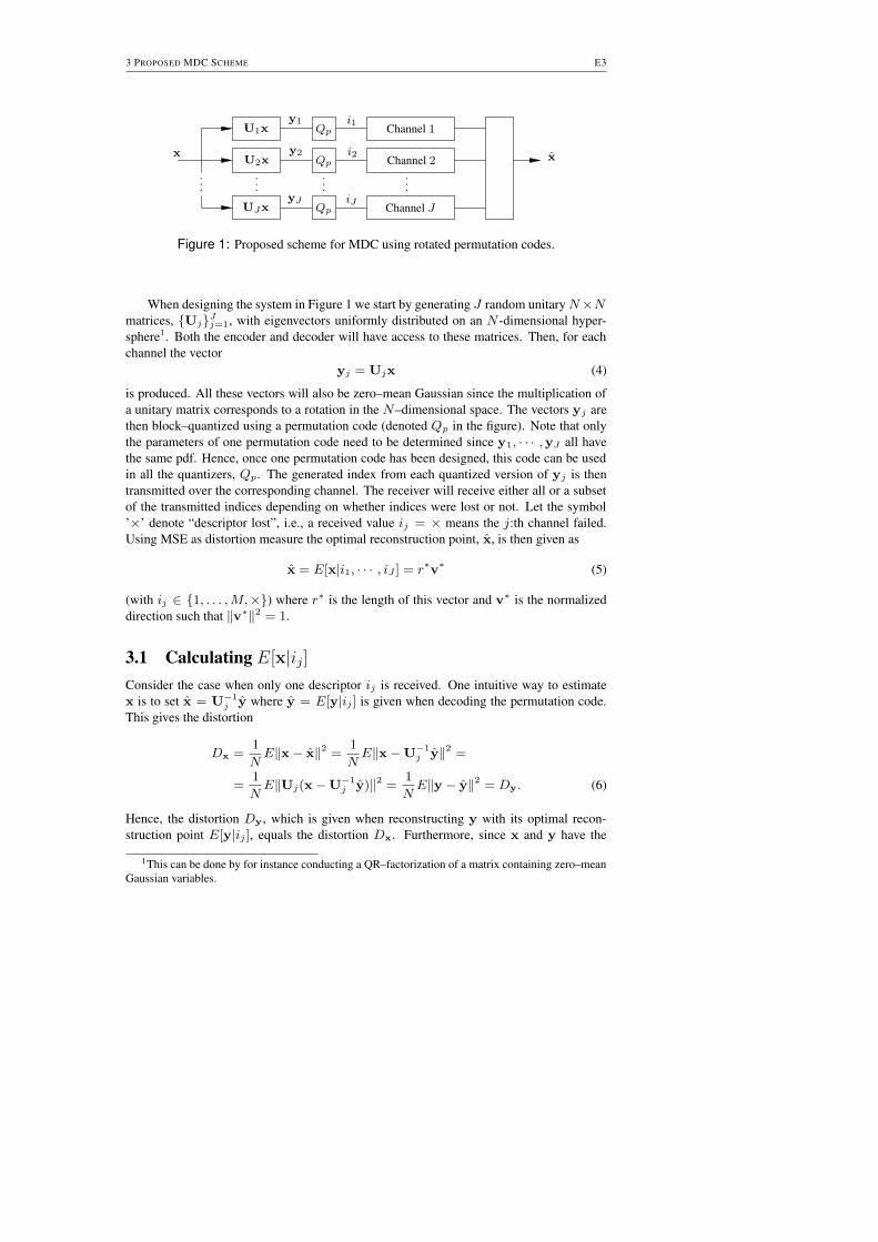
3 PROPOSED MDC SCHEME E3

PSfrag replacements

x x

U1x

U2x

UJx

......

......

Qp

Qp

Qp

i1

i2

iJ

y1

y2

yJ

Channel 1

Channel 2

Channel J

Figure 1: Proposed scheme for MDC using rotated permutation codes.

When designing the system in Figure 1 we start by generating J random unitary N×Nmatrices, {Uj}J

j=1, with eigenvectors uniformly distributed on an N -dimensional hyper-sphere1. Both the encoder and decoder will have access to these matrices. Then, for eachchannel the vector

yj = Ujx (4)

is produced. All these vectors will also be zero–mean Gaussian since the multiplication ofa unitary matrix corresponds to a rotation in the N–dimensional space. The vectors yj arethen block–quantized using a permutation code (denoted Qp in the figure). Note that onlythe parameters of one permutation code need to be determined since y1, · · · ,yJ all havethe same pdf. Hence, once one permutation code has been designed, this code can be usedin all the quantizers, Qp. The generated index from each quantized version of yj is thentransmitted over the corresponding channel. The receiver will receive either all or a subsetof the transmitted indices depending on whether indices were lost or not. Let the symbol’×’ denote “descriptor lost”, i.e., a received value ij = × means the j:th channel failed.Using MSE as distortion measure the optimal reconstruction point, x, is then given as

x = E[x|i1, · · · , iJ ] = r∗v∗ (5)

(with ij ∈ {1, . . . , M,×}) where r∗ is the length of this vector and v∗ is the normalizeddirection such that ‖v∗‖2 = 1.

3.1 Calculating E[x|ij]Consider the case when only one descriptor ij is received. One intuitive way to estimatex is to set x = U−1

j y where y = E[y|ij ] is given when decoding the permutation code.This gives the distortion

Dx =1

NE‖x − x‖2 =

1

NE‖x − U

−1j y‖2 =

=1

NE‖Uj(x − U

−1j y)‖2 =

1

NE‖y − y‖2 = Dy. (6)

Hence, the distortion Dy, which is given when reconstructing y with its optimal recon-struction point E[y|ij ], equals the distortion Dx. Furthermore, since x and y have the

1This can be done by for instance conducting a QR–factorization of a matrix containing zero–meanGaussian variables.

E4 MULTIPLE DESCRIPTION CODING USING ROTATED PERMUTATION CODES

PSfrag replacements

x1

x2

E[x|i1]

E[x|i2]

E[x|i1, i2]

i1

i2

Figure 2: Illustration of the basic idea. Each received descriptor will describe apossible N–dimensional volume that x belonged to. In this case wehave 2 dimensions.

same distribution we conclude that also x must have been an optimal reconstruction point.Hence,

E[x|ij ] = U−1j E[y|ij ]. (7)

3.2 Calculating E[x|i1, · · · , iJ ]

We will now think of the received indices as descriptions of volumes in an N–dimensionalspace. To explain this idea, consider the example, illustrated in Figure 2, with a permutationcode using the parameters N = 2, n1 = n2 = 1. Also assume J = 2 and U1 = I2 whereI2 is the 2–unitary matrix. Receiving i1 will in this case describe whether x1 ≤ x2 orx2 < x1 corresponding to a volume which we will denote V1. Hence, i1 tells us thatx ∈ V1 which gives the optimal reconstruction point as E[x|i1] = E[x|x ∈ V1]. In thesame manner also i2 will describe a volume, V2, such that x ∈ V2. This volume willhowever be different from V1 due to the random rotation. In the case that both i1 andi2 are received we know that x ∈ V1 ∩ V2 and we get the optimal reconstruction pointE[x|i1, i2] = E[x|x ∈ V1 ∩V2]. In general, each received index ij will describe a volumeVj and since all channels use the same permutation code all of these volumes will have equalvolume (except in the case of a lost descriptor; ij = × gives Vj = R

N and E[x|ij ] = 0).This gives

E[x|i1, · · · , iJ ] =V1∩···∩VJ

xf(x)dxV1∩···∩VJ

f(x)dx≈ 1

J ′

J�j=1

E[x|ij ] = rv (8)

where J ′ is the number of received (i.e. “nonlost”) packets, r is the length of the resultingvector and v is the normalized direction such that ‖v‖2 = 1. The approximation doneby averaging between all different reconstruction points makes intuitive sense, in Figure2 the resulting point is symbolized by a circle. This approximation is further motivatedby the results presented in the appendix where we, for the example illustrated in Figure 2,derive upper and lower bounds on the length r∗ of the optimal reconstruction point in (5).Furthermore, for the general case we have managed to show an upper bound and we conject

3 PROPOSED MDC SCHEME E5

0 20 40 60 80 1000

2

4

6

8

10UpperLower

PSfrag replacements

R

D0

N

r∗

(a)

1 2 3 410−2

10−1

100

J=2, N=5J=25, N=5J=2, N=200

PSfrag replacements

R

D0

N

r∗

(b)

Figure 3: (a) The upper and lower limits for r∗ when R = 2.5bits/symbol/channel. (b) The effect of the random matrix genera-tion for J = 2, N = 5 (crosses), J = 25, N = 5 (asterisk) andJ = 2, N = 200 (boxes).

a lower bound accordingly to7889 K�i=1

niµ2i ≤ r∗ ≤

√2σΓ " N+1

2 #Γ " N

2# (9)

where Γ(·) is the gamma function. In Figure 3(a) we show these bounds when R = 2.5bits/symbol/channel. Increasing the rate will make the gap between the lower and upperbound smaller and decreasing the rate will increase the gap. We also note that

r2 = ����� 1

J

J�j=1

E[x|ij ] ����� 2 =1

J2 :::::J�

j1=1

J�j2=1

E[x|ij1 ]T E[x|ij2 ] ::::: ≤≤ 1

J2

J�j1=1

J�j2=1 :::E[x|ij1 ]T E[x|ij2 ] ::: ≤ K�

i=1

niµ2i (10)

meaning that the length of the vector yielded by (8) is shorter, or equal, then the lowerbound of the optimal length in (9). We therefore replace the length r by the lower boundgiving the final formula for estimating x as

E[x|i1, · · · , iJ ] ≈ � K�i=1

niµ2i � 1

2

v. (11)

It was also verified in our simulations that this modification of the vector length gave a smallincrease in performance.

E6 MULTIPLE DESCRIPTION CODING USING ROTATED PERMUTATION CODES

10−3 10−2 10−1 1001

2

3

4

5

6D1 permD0 perm

PSfrag replacementsR

D

(a)

10−1 10010−3

10−2

10−1

MDSQPerm MDCECMDSQ

PSfrag replacements

D0

D1

(b)

Figure 4: (a) Comparing D0 (solid line) and D1 (dashed line) for the sug-gested method. (b) Studying the relation between D0 and D1 forSMDQ (crosses), ECSMDQ (circles), MDC based on permutationcodes (pentagrams) and the theoretical bound of [7] (solid line).

3.3 The Effect of the Generating Random MatricesSince the matrices {Uj}J

j=1 are generated in a random fashion one might expect that dif-ferent outcomes of this generation process will correspond to varying the performance ofthe system. However, our simulations indicate that when J and/or N grows large the per-formance converges to a fixed value. This is illustrated in Figure 3(b) where we analyzethe performance of 10 different realizations of the system, hence we try 10 different setsof randomly generated matrices, when receiving all J descriptions. This is done for threecases, in the first (crosses) we use J = 2, N = 5. From the plot we see that for this case theperformance of the different realizations become quite different meaning that some of thegenerated matrices are better than others. In the second case (asterisk) we increase J suchthat J = 25, N = 5. For this case it appears to be no greater difference in performancebetween the different realizations. This seems to be the case also for the third case (boxes)when we instead increase N such that J = 2, N = 200. We consider the proposed methodto be most interesting when using large N and moderate values for J corresponding to thethird case. Hence, the conclusion is that for our purposes generating the rotation matricesat random works satisfyingly.

4 SimulationsIn the simulations we use i.i.d. zero–mean Gaussian source data with σ2 = 1, J = 2 and forthe permutation codes N = 1000. It should be noted that the rate, R, is defined per channel,that is the unit is bits/symbol/channel. In Figure 4(a) we study the the usefulness of (11) bycomparing the central distortion D0, achieved when both descriptors are received, and theside distortion D1, achieved when only one descriptor is received, for different rates. It isclear that receiving an extra descriptor will improve the performance. We also see the effect

4 SIMULATIONS E7

PSfrag replacements

x x

−x Qp

Qp

i1

i2Enc.

ε1

ε2ε

Channel 1

Channel 2

Figure 5: Proposed structure for improving the performance of D0.

that the permutation code stops to improve above a certain rate and in Figure 4(a) and thiseffect starts to become visible around R = 4. However, this ’saturation’ level can be movedto a higher value of R by increasing N (see [10]).

We have also compared the proposed method with two well-known MDC meth-ods: multiple description scalar quantization (MDSQ) [1] and entropy-constrained MDSQ(ECMDSQ) [2]. The comparision with MDSQ may seem a bit unfair since MDSQ use asmall block size. However, using a much higher dimension in our scheme based on permu-tation coding will not necessarily give better performance and allowing for straightforwardimplementation of high-dimensional MDC is one of the main strengths of the suggestedmethod. ECMDSQ is essentially a high-dimensional block coding scheme, since it (implic-itly) assumes perfect entropy coding on top of scalar quantization. As shown in [11] therate–distortion characteristics of permutation coding is equivalent to that of entropy codedscalar quantization, as N → ∞. Hence, permutation coding is in this sense equivalent toentropy coded scalar quantization which makes the comparison of the suggested method toECMDSQ relevant.

4.1 Introducing More Design ParametersIt is a well known fact that when performing two channel MDC there is a tradeoff betweenthe central distortion D0 and the side distortion D1 such that if D0 is decreased D1 must beincreased and vice versa (that is, assuming D0 is close to the best theoretical performancefor a given D1; see e.g. [7, 8]). Although the previous simulation indicated good perfor-mance for the proposed system one of its drawbacks, in it present form, is that it cannoteasily be adjusted to trace out the tradeoff between D0 and D1, while this can be donewhen using MDSQ or ECMDSQ by adjusting some design parameters. Although we con-sider the task of developing such flexibility for our method to be a topic for future work, wehere introduce a quite straightforward method to approach the tradeoff between central andside distortion. The proposed structure is shown in Figure 5 where the encoder works in thesame fashion as in Section 3 with the additional feature that it also decodes the coded data toget x based on i1 and i2, that is the estimate produced when none of the descriptors are lost.This estimate is now compared to the original vector x to create the error ε = x − x. TheN/2 first samples of this error vector create a sequence ε1 which is block quantized using apermutation code. This second permutation code will be designed using ε as training data.In the case that both descriptors are received we get x = 0.5E[x|i1] + 0.5E[x|i2] + ε. Ifonly one descriptor is received, for instance i1, we use x = E[x|i1] + ε1. Using the rateRε to quantize ε leaves the rate Rx = R − Rε for quantizing x. By increasing the value of

E8 MULTIPLE DESCRIPTION CODING USING ROTATED PERMUTATION CODES

Rε the performance in terms of D0 will be improved. In fact, setting Rε = R will divide x

into two blocks which are permutation coded and transmitted over one channel each.In Figure 4(b) the result of simulating the modified system is shown when R = 2

bits/symbol/channel. The proposed method (pentagrams) outperforms MDSQ but does notbeat ECMDSQ, except at the leftmost pentagram which corresponds the the case Rε = 0,that is, when only the the approach of Section 3 is used. We consider this to indicate that thebasic approach proposed in this paper is sound, while there may be further improvementspossible upon the modified system in Figure 5 to introduce the desired flexibility. It istherefore our intention for further work to investigate alternative approaches to achieveefficient tradeoff between side and central distortion.

5 ConclusionsA new method for multiple description coding has been introduced and analyzed. The newapproach was compared to two other well known techniques, and simulations indicatedthat for certain regions in the tradeoff between central distortion and side distortion theperformance of the new scheme is comparable to the best of the benchmarks methods.However, in other regions the performance degrades slightly and as a topic for future workwe intend to improve the new method in these regions.

AppendixWe will here derive an upper and lower bound on r∗ for the example illustrated in Figure2, hence N = 2, J = 2, n1 = n2 = 1. Finally, we will also discuss the lower and upperbounds for the general case. When doing so we will use hyperspherical coordinates suchthat

xk = r cos θk

k−16l=1

sin θl ∀k = 1, · · · , N − 1

xN = r

N−16l=1

sin θl (12)

and the Jacobian determinant for this transformation is

J = rN−1N−16p=1

(sin θp)N−p−1. (13)

As can be seen in Figure 2 the resulting intersection created by the received descriptionsi1 and i2 can be described as V∩ = V1 ∩ V2 = {x : 0 ≤ r, α1 ≤ θ ≤ α2}, whenusing polar coordinates. When deriving r∗ we can instead consider the area V ′∩ = {x :0 ≤ r, 0 ≤ θ ≤ α}, with α = α2 − α1, since f(x) is rotation invariant. Hence,

E[x1|x ∈ V ′∩] =V′∩

x1f(x)dxV′∩

f(x)dx= ∞0 α

0r cos θe

− r2

2σ2 rdθdr ∞0 α

0e− r2

2σ2 rdθdr=

sin α

α

√2σΓ( 3

2)

Γ( 22)

(14)

REFERENCES E9

and similar equations gives

E[x2|x ∈ V ′∩] =1 − cos α

α

√2σΓ( 3

2)

Γ( 22)

(15)

where Γ(·) is the Gamma function. From this we get r∗ as

‖E[x|x ∈ V∩]‖ =

√2 − 2 cos α

α

√2σΓ( 3

2)

Γ( 22)

(16)

which is a strictly decreasing function for α ∈ (0, π]. Hence, the smaller intersection, thelarger value of r∗. The upper bound on r∗ is therefore given in the limit when α → 0. Thelower bound is given from the case when the intersection is as large as possible, that is whenV1 = V2, corresponding to the case when only one description is received. This gives� µ2

1 + µ22 ≤ r∗ ≤

√2σΓ( 3

2)

Γ( 22)

. (17)

In general we have shown that the upper bound on r∗ is created by the smallest possibleintersection, Vε = {x : 0 ≤ r, 0 ≤ θi ≤ ε ∀i = 1..N − 1} when ε → 0. Using (12)–(13)this length is calculated below:

limε→0

‖E[x|x ∈ Vε]‖ =

= limε→0

∞0 ε0 · · ·ε0r cos θ1e

− r2

2σ2 rN−1N−1;p=1

(sin θp)N−p−1dθ1 · · · dθN−1dr

∞0 ε0 · · ·ε0e− r2

2σ2 rN−1N−1;p=1

(sin θp)N−p−1dθ1 · · · dθN−1dr

=

= limε→0

∞0 rNe− r2

2σ2 dr ∞0 rN−1e− r2

2σ2 dr ε

0cos θ1(sin θ1)

N−2dθ1 ε

0(sin θ1)N−2dθ1

=

=

√2σΓ " N+1

2#

Γ " N2 # (18)

where l’Hospital’s rule is used in the final step on the second part of the expression. For thelower bound we conject that it corresponds to the vector length when only one descriptionis received, hence � K�

i=1

niµ2i � 1

2

≤ r∗. (19)

(18)–(19) gives (9).

AcknowledgmentsThe authors wish to thank J. Jalden and K. Werner for interesting and helpful discussions.

E10 MULTIPLE DESCRIPTION CODING USING ROTATED PERMUTATION CODES

References[1] V. A. Vaishampayan, “Design of multiple description scalar quantizers,” IEEE Trans-

actions on Information Theory, vol. 39, no. 3, pp. 821–834, 1993.

[2] V. A. Vaishampayan and J. Domaszewicz, “Design of entropy-constrained multiple-description scalar quantizers,” IEEE Transactions on Information Theory, vol. 40, pp.245–250, January 1994.

[3] S. D. Servetto, V. A. Vaishampayan, and N. J. A. Sloane, “Multi description latticevector quantization,” in Proceedings IEEE Data Compression Conference, Snowbird,UT, March 1999, pp. 13–22.

[4] V. K. Goyal, J. Kovacevic, and M. Vetterli, “Multiple description transform coding:Robustness to erasures using tight frame expansion,” in Proceedings IEEE Int. Symp.Information Theory, Cambridge, MA, August 1998, p. 408.

[5] ——, “Quantized frame expansions as source-channel codes for erasure channels,” inProceedings IEEE Data Compression Conference, Snowbird, UT, March 1999, pp.326–335.

[6] V. Goyal, M. Vetterli, and N. Thao, “Quantized overcomplete expansions in Rn: anal-

ysis, synthesis, and algorithms,” IEEE Transactions on Information Theory, vol. 44,pp. 16–31, January 1998.

[7] L. Ozarow, “On a source coding problem with two channels and three receivers,” BellSyst. Tech. J., vol. 59, no. 10, pp. 1909–1921, December 1980.

[8] A. E. Gamal and T. Cover, “Achievable rates for multiple descriptions,” IEEE Trans-actions on Information Theory, vol. 28, no. 6, pp. 851–857, November 1982.

[9] D. Slepian, “Permutation modulation,” Proc. IEEE, vol. 53, pp. 228–236, March 1965.

[10] T. Berger, F. Jelinek, and J. Wolf, “Permutation codes for sources,” IEEE Transactionson Information Theory, vol. 18, no. 1, pp. 160–169, January 1972.

[11] T. Berger, “Optimum quantizers and permutation codes,” IEEE Transactions on Infor-mation Theory, vol. 18, no. 6, pp. 759–765, November 1972.

Paper F

Improved Quantization in Multiple Description Coding byCorrelating Transforms

Niklas Wernersson, Tomas Skollermo and Mikael SkoglundPublished in Proceedings IEEE Workshop on Multimedia Signal Processing 2004

c©2004 IEEEThe layout has been revised

Improved Quantization in Multiple DescriptionCoding by Correlating Transforms

Niklas Wernersson, Tomas Skollermo and Mikael Skoglund

Abstract

The objective with Multiple Description Coding (MDC) is to code one source of datainto multiple bitstreams. The coding is done in such a way that multiple levels of quality isachieved. This means that even if one or a few of the bitstreams are lost, the received bitsshould make it possible to get an approximated version of the original data. One way todo this is to use pairwise correlating transforms which will introduce correlation betweenthe bitstreams. This correlation can be used in order to get an estimate of a lost stream.In this paper a new approach for MDC using pairwise correlating transforms is presented.In this approach, contrary to previous work, quantization of the source data is performedafter the data has been transformed. This makes it possible to improve the shape of thequantization cells and to tailor these to the employed transform. We demonstrate that thisoffers a substantial performance gain compared with previous approaches to MDC usingpairwise correlating transforms.

1 IntroductionPacket networks have gained in importance in recent years, for instance by the wide-spreaduse of the Internet. By using these networks large amounts of data can be transmitted. Whentransmitting for instance an image a current network system typically uses the TCP protocolto control the transmission as well as the retransmission of lost packages. Unfortunately,packet losses can in general not be neglected and this problem therefore has to be consideredwhen constructing a communication system. The compression algorithms in conventionalsystems quite often put quite a lot of faith into the delivery system which gives rise to someunwanted effects.

Suppose that N packets are used to transmit a compressed image and the receiver recon-structs the image as the packets arrive. A problem would arise if the receiver is dependenton receiving all the previous packets in order to reconstruct the data. For instance if pack-ets {1, 3, 4...N} are received it would be an undesirable property if only the informationin packet 1 could be used until packet 2 eventually arrives. This would produce delays inthe system and great dependency on the retransmission process. In the case of a real timesystem the use of the received packets may have been in vain because of a lost packet. One

F2 IMPROVED QUANTIZATION IN MULTIPLE DESCRIPTION CODING BY CORRELATING TRANSFORMS

−1

−1

Q

Q

Q

Q

PSfrag replacements

Estimator of

Estimator of

Transform transform

Channel 1

Channel 2

Inverse

A and B

A and Bfrom C

from D

A

A

A

B

B

B

C

D

A

BB

A

Q−1

Q−1

Figure 1: The basic structure of MDC using pairwise correlating transforms aspresented in [1].

way to deal with this is to use Multiple Description Coding (MDC) where each receivedpacket will increase the quality of the image no matter which other packets that have beenreceived, see e.g [1–8]. MDC will therefore enhance the reliability of the communicationsystem.

In this paper a new approach for MDC using pairwise correlating transform is presented.In previous work, e.g. [1], the data is first quantized and then transformed. We suggest toreverse the order of these operations, leading to performance gains. The optimal cell shapeof the transformed data relates to the optimal cell shape of the original data through somebasic equations which makes it possible to perform quantization and designing the code-words after the data is transformed. Only the case with two descriptors will be consideredbut the theory can easily be extended to handle more descriptors. It is assumed that only onedescriptor can be lost at a time (not both) and that the receiver knows when a descriptor islost. The two channels are also assumed to have equal failure probability, perror , and MSEis used as a distortion measure. The source signal is modelled as uncorrelated Gaussiandistributed.

This paper is organized as follows. In Section 2 some preliminary theory of MDCusing pairwise correlating transforms is discussed. In Section 3 the new approach for MDCusing pairwise correlating transforms is presented. In Sections 4 and 5 some results andconclusions will be presented.

2 PreliminariesGenerally the objective with transform coding is to remove redundancy in the data in orderto decrease the entropy. The goal of MDC is the opposite, namely to introduce redundancyin the data but in a controlled fashion. A quite natural approach for this is to first removepossible redundancy in the data by for instance using the Karhunen-Loeve transform. Afterthis MDC is used in order to introduce redundancy again, but this time in selected amounts.In this paper it is assumed that the original data is uncorrelated Gaussian distributed so the

2 PRELIMINARIES F3

problem of removing initial redundancy will not be considered.In Figure 1 the basic structure of the MDC described in [1] is shown. The data variables

A and B are to be transmitted and are quantized into A and B. These values are thentransformed using the transform 0 C

D 2 = T 0 A

B 2 , (1)

where T is a 2 × 2 matrix. This transform is invertible so that0 A

B 2 = T−1 0 C

D 2 . (2)

Once the data have been transformed C and D are transmitted over two different chan-nels. If both the descriptors are received the inverse transform from (2) is used in order toproduce A and B. However, if one of the descriptors is lost, A and B can be estimated fromthe other descriptor. This comes from the fact the the transform matrix T is nonorthogonaland introduces redundancy in the transmitted data. For instance, if the receiver receivesonly the descriptor C, (A, B) is estimated to E[(A, B)|C].

For the two descriptors case the transform matrix T, optimized according to [1], can bewritten as

T = 0 cos θ/√

sin 2θ sin θ/√

sin 2θ

− cos θ/√

sin 2θ sin θ/√

sin 2θ 2 = 0 a bc d 2 . (3)

where θ will control the amount of introduced redundancy.The values C and D that are to be transmitted should be integers which is not necessar-

ily the case in (1). Therefore the transform is implemented as follows (a, b, c and d are thevalues from (3) and [·] denotes rounding).

A = 0 A

Amax

qA + 0.5 2 , B = 0 B

Bmax

qB + 0.5 2 , (4)

W = B + 0 1 + c

dA 2 , (5)

D = [dW ] − A, (6)

C = W − 0 1 − b

dD 2 . (7)

It is assumed that A ∈ [0, Amax] and B ∈ [0, Bmax]. qA and qB are integers decidinghow many quantization levels there are for A and B respectively. It is also assumed, for theextremes, that 3 0

AmaxqA + 0.5

4is rounded to 1 and 3 Amax

AmaxqA + 0.5

4is rounded to qA.

Assuming that both descriptors are received in the decoder the corresponding inversetransform is performed as

W = C + 0 1 − b

dD 2 , (8)

A = [dW ] − D, (9)

B = W − 0 1 + c

dA 2 , (10)

F4 IMPROVED QUANTIZATION IN MULTIPLE DESCRIPTION CODING BY CORRELATING TRANSFORMS

A =(A − 0.5)Amax

qA

, B =(B − 0.5)Bmax

qB

. (11)

As mentioned before, if one of the descriptors is lost A and B are, depending on whichdescriptor that was lost, estimated to E[(A, B)|C] or E[(A, B)|D].

Note here that the number of quantization levels for A and B, qA and qB , will in generalnot equal the ones for C and D, qC and qD . (qA, qB) are however mapped to (qC , qD) bya function ϕ according to

ϕ : N2 −→ N2,ϕ(qA, qB) = (qC , qD).

(12)

Hence, if we want to transmit C and D using, e.g., 3 bits each we need to find qA and qB

so that ϕ(qA, qB) = (23, 23).From (4) it is seen that the described MDC system in (4)–(11) uses uniform quantiza-

tion. The system could easily be improved by introducing two nonuniform scalar quantizers,one for the A-values and one for the B-values. This improved system is what will be usedand considered further on in this paper. This leads to modifications of (4) and hence also(11). Using the MSE as a distortion measure a codebook could be designed by using forinstance the generalized Lloyd algorithm briefly explained in Section 3.

3 Improving the QuantizationIn brief the algorithm in Section 2 can be summarized as

1. Train encoder/decoder and quantize data. The encoder uses two scalar quantizers inorder to decrease the entropy of the data. This means that the data values are mappedonto a set of codevectors.

2. Transform the quantized data. Redundancy is introduced into the data by using (5)–(7).

3. Transmit data. The data is transmitted and packet or bit losses may occur, whichmeans that some descriptors may be lost.

4. Estimate lost data and do the inverse transform. This is done using (8)–(10).

In this paper we suggest to do this algorithm in a different order. Changing the order of Steps1 and 2 would mean that the transformation is done directly and training and quantization isdone on the transformed values. Naturally, also the order in the receiver has to be reversedappropriately.

Using MSE as the distortion measure a point in the data is quantized to the K:th code-vector according to

K = arg mink

�<0 AB 2 − 0 Ak

Bk 2 T �<0 AB 2 − 0 Ak

Bk 2 = arg min

k � 0 ∆Ak

∆Bk 2 T 0 ∆Ak

∆Bk 2 � , (13)

3 IMPROVING THE QUANTIZATION F5

where Ak and Bk are the coordinates of the different codewords. Using (2) this can also bewritten

K = arg mink

� T−1 �=0 CD 2 − 0 Ck

Dk 2 > T � T−1 �<0 CD 2 − 0 Ck

Dk 2 > = arg min

k

� T−1 0 ∆Ck

∆Dk 2 T � T−1 0 ∆Ck

∆Dk 2 = arg min

k � 0 ∆Ck

∆Dk 2 T

T−1T

T−1 0 ∆Ck

∆Dk 2 � . (14)

According to the discussion in Section 2 there should be qC quantization levels for C andqD quantization levels for D. Introducing this restriction in (14) and using (3) gives

(I, J) = arg mini,j

(∆C2i + 2 cos(2θ)∆Ci∆Dj + ∆D2

j ), (15)

where i ∈ {1, 2, . . . , qC} and j ∈ {1, 2, . . . , qD}. This equation will allow us to designa codebook for the transformed values instead of the original data. The generalized Lloydalgorithm can be used for this purpose. This algorithm is briefly summarized below.

1. Define initial codebook.

2. Quantize each data point to that codeword that minimizes the contribution to thedistortion.

3. For each codeword (if it is possible), find a new optimal codeword for all the valuesthat have been quantized to this particular codeword and update the codebook.

4. Until the algorithm converges go to Step 2.

For Step 2, (15) is used to quantize the data. In Step 3 we want to find an optimal codewordfor those values that have been quantized to a particular codeword. Calculating the partialderivative of the total distortion as

∂

∂CI

�(C,D)

(∆C2i + 2 cos(2θ)∆Ci∆Dj + ∆D2

j ) (16)

and minimizing by setting (16) equal to zero will give an equation for updating the code-vectors, namely

CI =1

NI

�∀(C,D):Q(C,D)=(CI ,Dj)

(C + cos(2θ)∆Dj). (17)

The sum is taken over all those points (C, D) which will be quantized to (CI , Dj) for agiven I and an arbitrary j. NI is the number of points within this set. In a similar mannerwe get

DJ =1

NJ

�∀(C,D):Q(C,D)=(Ci,DJ )

(D + cos(2θ)∆Ci) (18)

and this is done for I = 1, 2, . . . , qC and J = 1, 2, . . . , qD . Once the codebook hasbeen generated the encoder and decoder are ready to use. The data to be transmitted isthen transformed by the matrix T, quantized and transmitted. In the decoder the reverseprocedure is done. This is illustrated in Figure 2.

F6 IMPROVED QUANTIZATION IN MULTIPLE DESCRIPTION CODING BY CORRELATING TRANSFORMS

PSfrag replacements

AA

BB

C

D 0

0

0

0

0

0

1

2

2

2

2

2

2

34

4

4

4

4

4

5

6 66

−1−2

−2

−2

−2

−2

−2

−3 −4

−4

−4

−4

−4

−4−5 −6 −6−6

Figure 2: In the left plot the original set of data is shown. These values are firsttransformed and then quantized as shown in the middle plot. In thereceiver the inverse transform is used as shown in the right plot. Inthis plot also the corresponding quantization cells are illustrated.

4 Simulation ResultsIn order to compare the system explained in Section 2 and [1] with the new system intro-duced in Section 3 these were implemented and simulated. Uncorrelated zero mean Gaus-sian data was generated and used to train the encoders/decoders and then to simulate thesystems. In the simulations presented here the source data A and B have equal variances.Similar results have however been obtained also for the case of nonequal variances. Asmentioned in Section 1 it is assumed that only one descriptor can be lost at a time and thatthe receiver knows when a descriptor is lost. The angle for the transform matrix T used inthe simulations was θ = π

5. The result is presented in Figure 3. perror shows the proba-

bility that one of the descriptors is lost and the y-axis shows the signal–to–distortion ratio,defined as 10 log E[x2]

E[(x−x)2], where x is the data signal and x is the reconstructed signal. In

Figure 3(a) both C and D were transmitted using 3 bits each which gives qC = qD = 23.In order to accomplish this (qA, qB) had to be identified so that ϕ(qA, qB) = (23, 23). Thiswas found to be true for qA = 5 and qB = 7. Similar results are shown in Figures 3(b) and3(c) when using 4 and 8 bits.

As can be observed in Figure 3 the new system outperforms the original system forall investigated values of perror . In the case of 3 bits per description, as shown in Figure3(a), the advantage of the new scheme is more noticeable at low packet loss rates. Inparticular we see that as perror → 0 the new system outperforms the original scheme byabout 2 dB. When using 4 bits per description, as in Figure 3(b), we notice that the gainof the new approach is more-or-less constant over the range of different packet loss rates.Finally, studying Figure 3(c), we can observe that in the case of 8 bits per description thesituation has changed and the gain is now more prominent at high packet error rates. Insummary we see that in all cases considered there is a constant gain at medium to highpacket loss rates and this gain increases with the transmission rate of the system, while at

5 CONCLUSIONS F7

0 0.2 0.4 0.6 0.8 12

4

6

8

10

12

14

16

PSfrag replacements

perror

10lo

gE

[x2]

E[(

x−

x)2

]

(a)

0 0.2 0.4 0.6 0.8 10

5

10

15

20

PSfrag replacements

perror

10lo

gE

[x2]

E[(

x−

x)2

]

(b)

0 0.2 0.4 0.6 0.8 10

5

10

15

20

25

PSfrag replacements

perror

10lo

gE

[x2]

E[(

x−

x)2

]

(c)

Figure 3: The solid line shows the performance of the original system [1] andthe dashed line shows that of the new system, in terms of signal-to-distortion ratio versus packet loss rate, perror . C and D are transmit-ted using (a) 3, (b) 4 and (c) 8 bits each and θ = π

5.

low packet loss rates there is an additional gain at low rates (as in Figure 3(a)) and hardlyno gain at high rates (as in Figure 3(c)). One possible explanation for this behavior is thatthe new approach in particular improves the performance at low transmission and packetloss rates due to the improved optimization of the individual quantizers. At high loss ratesthis gain is less pronounced, since when packet losses occur the redundancy introduced bythe linear transform has an equal or higher influence on the total performance than has theperformance of the individual quantizers.

5 ConclusionsA new MDC method has been introduced. The method is developed from an extendedversion of the MDC using pairwise correlating transforms described in [1]. Using the orig-inal method the data is quantized and then transformed by a matrix operator in order to

F8 IMPROVED QUANTIZATION IN MULTIPLE DESCRIPTION CODING BY CORRELATING TRANSFORMS

increase the redundancy between descriptors. In the new suggested method the data is firsttransformed and then quantized. In Section 3 it is shown that this transform leads to a mod-ification of the distortion measure. Using the generalized Lloyd algorithm when designingthe quantization codebook also leads to a new way to update the codevectors. In section4 simulations were done that shows that the new method performs better than the originalone when smaller amounts of redundancy are introduced into the transmitted data. For thesimulations conducted in Section 4, using θ = π

5, the new method gave 2 dB gain compared

to the original system when no descriptors were lost. The gain decreased to about 0.5-1 dBwhen the probability of lost descriptors was increased.

References[1] Y. Wang, M. Orchard, V. Vaishampayan, and A. Reibman, “Multiple description cod-

ing using pairwise correlation transforms,” IEEE Transactions on Image Processing,vol. 10, no. 3, March 2001.

[2] V. K. Goyal and J. Kovacevic, “Generalized multiple description coding with correlat-ing transforms,” IEEE Transactions on Information Theory, vol. 47, no. 6, pp. 2199–2224, sep 2001.

[3] V. K. Goyal, “Multiple description coding: Compression meets the network,” IEEESignal Processing Magazine, vol. 18, pp. 74–93, sep 2001.

[4] V. A. Vaishampayan, “Design of multiple description scalar quantizers,” IEEE Trans-actions on Information Theory, vol. 39, no. 3, pp. 821–834, 1993.

[5] S. Pradhan, R. Puri, and K. Ramchandran, “n-channel symmetric multiple descriptions-part i:(n, k)source-channel erasure codes,” IEEE Transactions on Information Theory,vol. 50, no. 1, pp. 47–61, January 2004.

[6] P. Koulgi, S. Regunathan, and K. Rose, “Multiple description quantization by deter-ministic annealing,” IEEE Transactions on Information Theory, vol. 49, no. 8, pp. 2067– 2075, August 2003.

[7] R. Venkataramani, G. Kramer, and V. Goyal, “Multiple description coding with manychannels,” IEEE Transactions on Information Theory, vol. 49, no. 9, pp. 2106–2114,September 2003.

[8] P. Dragotti, S. Servetto, and M. Vetterli, “Optimal filter banks for multiple descriptioncoding: analysis and synthesis,” IEEE Transactions on Information Theory, vol. 48,no. 7, pp. 2036 – 2052, July 2002.

Paper G

On Source Decoding Based on Finite-Bandwidth SoftInformation

Niklas Wernersson and Mikael SkoglundPublished in Proceedings of IEEE International Symposium on Information Theory 2005

c©2005 IEEEThe layout has been revised

On Source Decoding Based on Finite-Bandwidth SoftInformation

Niklas Wernersson and Mikael Skoglund

Abstract

Designing a communication system using joint source–channel coding in general makesit possible to achieve a better performance than when the source and channel codes are de-signed separately, especially under strict delay-constraints. The majority of work done injoint source-channel coding uses a discrete channel model, corresponding to an analogchannel in conjunction with a hard decision modulation scheme. The performance of sucha system can however be improved by using soft decision modulation. The main cost is ahigher decoding complexity. An alternative is to quantize the soft information and store thepre-calculated soft decision values in a lookup table. In this paper we propose new meth-ods for quantizing soft channel information, to be used in conjunction with soft-decisionsource decoding. We achieve a performance close to that of a system using unquantized softinformation.

1 IntroductionWireless distribution of multimedia has gained in importance in recent years. This has led toa number of different methods and standards, suitable for transmission, when representingaudio, video, speech and images. A question of great interest is how to make the tradeoffbetween designing efficient source codes and designing channel codes robust toward trans-mission errors. This has made the area of joint source–channel coding of particular interestsince it in general makes it possible to get a higher performance than if the source and chan-nel codes are designed separately. Most of the work done in joint source-channel codinguses a discrete channel model, that is an analog channel in conjunction with a hard decisionmodulation scheme. Using soft decision modulation can however improve the performanceof such a system.

There are several previous works that investigate source coding with decoding based ondifferent kinds of soft decision modulation, e.g. [1–5]. While [1–3] assumed unquantizedsoft channel output-values, the work in [4, 5] was based on quantized soft information.More precisely, [4, 5] presented a scheme based on channel optimized vector quantization(COVQ), see e.g. [6–8], over a binary-input Gaussian channel and using uniform scalarquantization to quantize the soft channel outputs, resulting in a discrete memoryless channel

G2 ON SOURCE DECODING BASED ON FINITE-BANDWIDTH SOFT INFORMATION

with two inputs and 2q outputs. The main motivation in [4, 5] for working with quantizedsoft information was to reduce the decoding complexity compared e.g. with the decoderpresented in [2], since over a discrete channel decoding can be based on a look-up table.

The present work is partly an extension of [4, 5] to using non-uniform quantizationand vector quantization (VQ) to represented soft channel information. Our main motivationis however a scenario where the soft channel output information has to be bandlimited inorder to be further conveyed to a node where it is used in soft source decoding. Consider, forexample, applications where the transmitting node connects to a wired network via wirelessaccess to a basestation, and where the receiving entity is connected to the wired network.The basestation will then have to limit the resolution of the received soft information inorder to transport it to the receiving node. In practice the wired part of the network canoften be assumed to be error-free, since it is implemented using high-reliability coppercables or optical fiber. Still, the receiving node may use soft information transported fromthe receiving basestation to counteract the effects of noise and signal fading in the wirelesspart of the connection.

Referring to a generic scenario similar to the one described above, we discuss two mainissues: a) How to represent the soft information available at the basestation, the main al-ternatives being to re-quantize soft source estimates or to quantize the soft channel outputsdirectly, and; b) In the case of quantized soft channel values, different means of quantiza-tion, including non-uniform scalar quantization and vector quantization.

The paper is organized as follows. In Section 2 the problem is illustrated and explained.Three different approaches for transmitting bandlimited soft information is suggested. InSection 3 these three approaches are analyzed. An expression for scalar quantization of softchannel values is also derived. In Sections 4 and 5 some results and conclusions will bepresented.

2 Problem formulationWe are considering the problem illustrated in Figure 1. A random vector X ∈ R

d is vec-tor quantized and transmitted over a wireless channel denoted Channel 1. The channel ismodeled as a Gaussian channel and the transmission is done using BPSK. The m outputbits from the encoder, represented by i ∈ {−1, +1}m, are corrupted by the noise n ∈ R

m.Hence, Receiver 1 measures r ∈ R

m according to

r = i + n (1)

where n is zero mean white Gaussian noise with covariance matrix Cn = σ2In, where In

is the n-unity matrix.Receiver 1 wishes to pass on the data represented by r to an other unit, Receiver 2,

and this is assumed done over an error-free connection, e.g. via optical fiber. The link fromReceiver 1 to 2 is assumed to be of high but finite bandwidth, and the transmission needstherefore to be limited to qm bits per received r. This means that a vector j ∈ {0, 1}qm

will be transmitted and finally received by Receiver 2. In Receiver 2 j is used in order toget X = Xj which is an estimate of X.

The encoder can be designed using source optimized vector quantization (SOVQ) wherethe mean-square error (MSE) between the source data X and the quantized source datarepresented by i is minimized, based e.g. on the generalized Lloyd algorithm [9]. However,

2 PROBLEM FORMULATION G3

PSfrag replacementsX ∈ R

d

Encoderi ∈ {−1, +1}m

n ∈ Rm

Channel 1

r ∈ Rm

Receiver 1

Receiver 2j ∈ {0, 1}qm

Channel 2

X ∈ Rd

Figure 1: X is transmitted to Receiver 1 using m bits. The bits are corruptedby the noise n. In Receiver 1 the soft information contained in r hasto be bandlimited to qm bits, represented by j, which are transmittedto Receiver 2. Finally X is estimated from j.

since the transmission will constitute a random Markov-chain, the overall performance canbe improved using COVQ. In the COVQ approach, we know from e.g. [6–8] that for a fixedencoder, represented by the encoder regions {Si}, such that X ∈ Si =⇒ transmit index i,the optimal reconstruction value when j is received is

Xj = E[X|j]. (2)

That is, for a fixed encoder these vectors should be used for decoding. Furthermore, whenthe decoder is known and fixed the encoder regions that minimize the overall distortion are

Si = {x :�j

P (j|i)‖X − Xj‖2 ≤�j

P (j|i′)‖X − Xj‖2, ∀i′}. (3)

The expressions (2) and (3) together specify local optimality of a COVQ and by trainingthe system in an iterative fashion using these equations the encoder and decoder can bedesigned [6–8]. Both SOVQ and COVQ will be investigated for the system described inFigure 1.

Our main interest in this paper concerns how to best make use of the soft informa-tion contained in r, under the constraint that Receiver 1 has to compress r into the finite-bandwidth representation j. Three different approaches are suggested and explained in thefollowing subsections.

2.1 Re-Quantization of a Soft Source EstimateFrom estimation theory it is a well known fact that the optimal decoder that minimizesthe MSE distortion between the decoded value X, estimated from the unquantized soft

G4 ON SOURCE DECODING BASED ON FINITE-BANDWIDTH SOFT INFORMATION

information in r, and the original data X is given as

X = E[X|r] =

�xfx|r(x|r)dx. (4)

Based on this, one way to implement the system in Figure 1 is as shown in Figure 2.PSfrag replacements

E[X|r] VQr ∈ R

m j ∈ {0, 1}qm

Channel 2

X ∈ Rd

Figure 2: Structure of the first approach. All the soft information is used whencalculating E[X|r]. This value is then vector quantized in order tomeet with the condition of limited bandwidth at Channel 2.

In this approach all the soft information in r is used in order to calculate the soft valueE[X|r]. This value is then vector quantized, in order to meet with the condition of a limitedbandwidth, in such a way that the distortion of the reconstructed value is minimized. Addi-tional distortion will hence be introduced in the final reconstructed value X, compared withX.

2.2 Vector Quantization of the Soft Channel Values

Here we propose to quantize the “soft bits” represented by the components of r, in sucha way that the distortion between X and X is minimized. The basic structure is shown inFigure 3. This leads to that r is quantized into one of 2qm quantization cells. The indexof this quantization cell is transmitted over Channel 2 and in Receiver 2 the reconstructionvalue X is computed.PSfrag replacements

E[X|j]VQr ∈ R

m j ∈ {0, 1}qm

Channel 2

X ∈ Rd

Figure 3: Structure of the second approach. The soft information in r is vectorquantized and transmitted over Channel 2. In the final receiver X iscalculated as X = E[X|j].

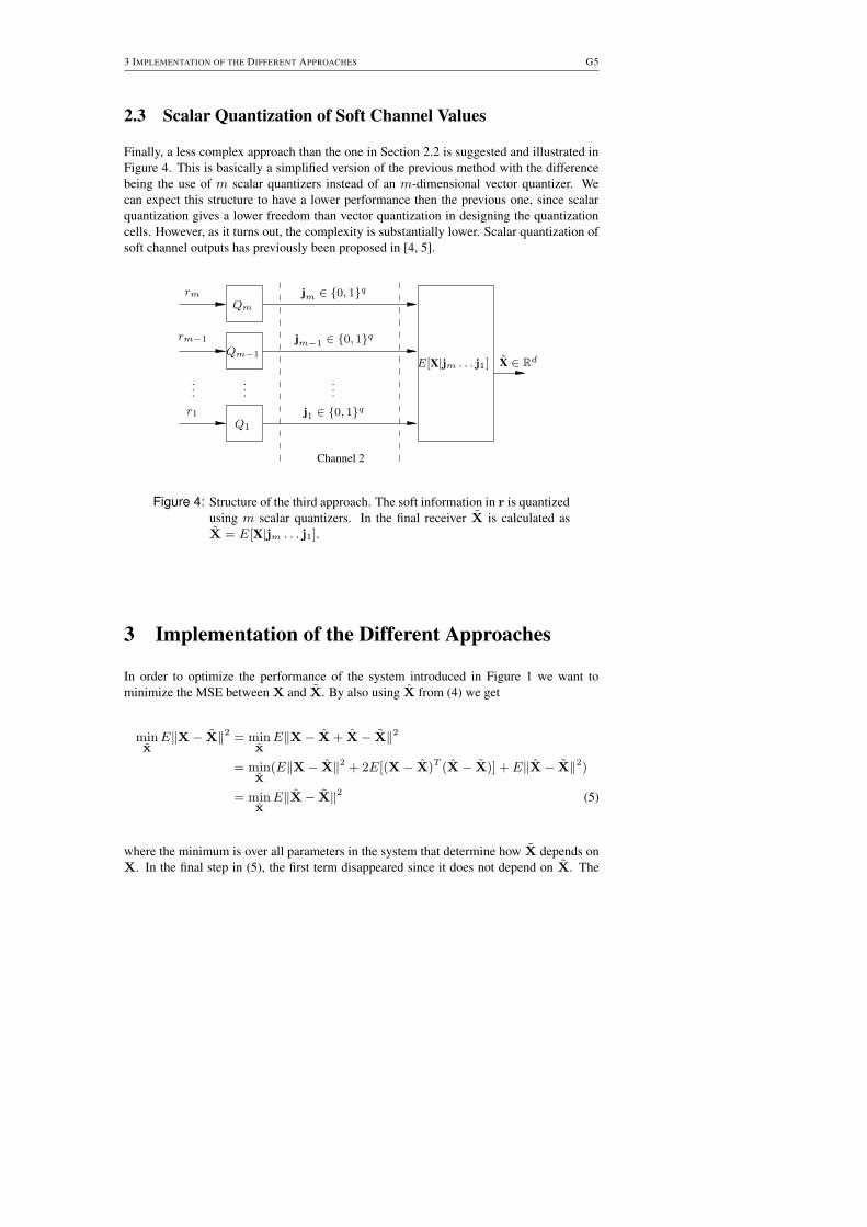
3 IMPLEMENTATION OF THE DIFFERENT APPROACHES G5

2.3 Scalar Quantization of Soft Channel Values

Finally, a less complex approach than the one in Section 2.2 is suggested and illustrated inFigure 4. This is basically a simplified version of the previous method with the differencebeing the use of m scalar quantizers instead of an m-dimensional vector quantizer. Wecan expect this structure to have a lower performance then the previous one, since scalarquantization gives a lower freedom than vector quantization in designing the quantizationcells. However, as it turns out, the complexity is substantially lower. Scalar quantization ofsoft channel outputs has previously been proposed in [4, 5].

PSfrag replacements

E[X|jm . . . j1]

Qm

Qm−1

Q1

......

...

rm

rm−1

r1

jm ∈ {0, 1}q

jm−1 ∈ {0, 1}q

j1 ∈ {0, 1}q

Channel 2

X ∈ Rd

Figure 4: Structure of the third approach. The soft information in r is quantizedusing m scalar quantizers. In the final receiver X is calculated asX = E[X|jm . . . j1].

3 Implementation of the Different Approaches

In order to optimize the performance of the system introduced in Figure 1 we want tominimize the MSE between X and X. By also using X from (4) we get

minX

E‖X − X‖2 = minX

E‖X − X + X − X‖2

= minX

(E‖X − X‖2 + 2E[(X − X)T (X − X)] + E‖X − X‖2)

= minX

E‖X − X‖2 (5)

where the minimum is over all parameters in the system that determine how X depends onX. In the final step in (5), the first term disappeared since it does not depend on X. The

G6 ON SOURCE DECODING BASED ON FINITE-BANDWIDTH SOFT INFORMATION

second term equals zero since

E[(X − X)T (X − X)] = E ? E[(X − X)T (X − X) | r ] @= E ? (X − X)T E[(X − X)|r] @= E[(X − X)T

0] = 0 (6)

Note that (5) implies that minimizing the MSE between X and X is actually equivalentto minimizing the MSE between X and X.

3.1 Re-Quantization of a Soft Source EstimateBased on (5) we see that the quantizer in Figure 2 should be constructed in such a way thatE[‖X− X‖2] is minimized. This means that the quantizer can be trained just as in regularVQ training where E[‖X − X‖2], with X = X(r) = E[X|r], is the distortion measureand X is encoded as

J = arg minj

(E[‖X − Xj‖2|r]) (7)

where J denotes the (random) integer representation of the binary index j. When imple-menting (7) it is assumed that a decoder X = Xj , when J = j, is fixed. For a fixedencoder, represented by (7), optimal decoding is done according to

Xj = E[X|J = j]. (8)

From these equations it is seen that any given distribution of X together with a given σ2

will generate a distribution of X witch will decide how the quantizer should be designed.

3.2 Vector Quantization of the Soft Channel ValuesIn this approach we want to vector quantize the received r into one of 2qm different rep-resentations rj . After the quantization the index J is transmitted over the channel and thereconstruction value X(rj) = E[X|rj ] is calculated. The problem is to find the differentrj’s such that E[‖X− X‖2], with X = Xj = X(rj), is minimized. For an observed valueof r, the encoding should hence be done according to

J = arg minj

E ? ‖X(r) − X(rj)‖2 | r @ = arg minj

E ? ‖X(r) − Xj‖2 | r @ . (9)

This is the same encoder as in (7), which means that the two approaches, in this sense, areequivalent. That is, it does not matter whether we consider encoding r into j as a problemin the “X domain” or in the “r domain.” This further means that the third approach, definedin Figure 4, can not have a better performance than the system in Figure 2.

The structure of the quantization cells obtained based on (9) is illustrated in Figure 5 fora simple example with m = 2, q = 2 and d = 1. For demonstration purposes, the exampleassumes that X is discrete and uniformly distributed over {1, 2, 3, 4}, and these four valuesare transmitted as i ∈ {(±1,±1)}. The noise variance is σ2 = 0.5. As can be seen inthis figure the shape of the quantization cells is quite complex. It is interesting to note thatdifferent r’s can be quantized to the same cell although they are quite far from each other.For instance we see that (r1, r2) = (0,−1.5) and (r1, r2) = (−1, 1) will be quantized tothe same cell. This effect comes from the soft decoding. Since (r1, r2) = (0,−1.5) liesjust between two possible codewords the reconstruction value is essentially chosen as themean of these.

3 IMPLEMENTATION OF THE DIFFERENT APPROACHES G7

PSfrag replacements1.5

0.5

0

0

−0.5

−1

−1−1.5

1

1

1 2

3 4

r 1

r2

Figure 5: The shape of quantization cells obtained based on (9) when m = 2,q = 2 and d = 1. The different X-values are {1, 2, 3, 4}, with equalprobabilities, and the noise variance σ2 = 0.5.

3.3 Scalar Quantization of Soft Channel ValuesAs previously stated this method will have a lower performance than the ones suggested inSections 2.1 and 2.2. However, the complexity is substantially lower which still makes themethod interesting. In order to minimize E[‖X − X‖2], in Figure 4, when quantizing rk

to jk the encoding should be done according to

Jk = arg minjk

E ? ‖X(rm, . . . , r1) − X(jm, . . . , j1)‖2 | rk, jk @ (11)

Also, for fixed encoders the optimal reconstructed value X(jm, . . . , j1) is obtained as

X(jm, . . . , j1) = E[X|jm, . . . , j1]. (12)

The expressions in (11)–(12) make it possible to train the quantizers in an iterativefashion. It is readily seen that implementing (11) requires knowledge of the pdf for X.Otherwise the expected value needs to be estimated from a training set of data. This problemis also encountered when calculating (12).

In the next section optimal design of the scalar quantizers will be compared to thefollowing alternatives:

• Hard decision. This is the classical hard-decision source decoding approach, wherea hard decision is made on all ri’s such that a negative ri gives −1 and vice versa.

• The Lloyd approach. A quite intuitive way to quantize the data is to minimizethe MSE of the reconstructed ri. That is, to design ri such that E[‖r − ri‖2] isminimized. However, when discussing Figure 5 it was concluded that the nearestneighbor criterion is not necessarily suitable, due to the complex shape of the cellsbased on (7). In the Lloyd approach, we base the decoding on (12), meaning that

G8 ON SOURCE DECODING BASED ON FINITE-BANDWIDTH SOFT INFORMATION

0 1 2 3 4 5 6 7 8−1

0

1

2

3

4

5

6

7

8

9Soft decisionApproach AOptimized quantizerUniform quantizerThe Lloyd approachHard decision

PSfrag replacements

SNR

Sign

al–t

o–D

isto

rtio

n–R

atio

(dB

)Figure 6: Results of the SOVQ system when X is 2-dimensional Gaussian un-

correlated, m = 4 and q = 2. As can be seen the performance gainfrom using the optimal scalar quantizers over the uniform quantizersis minor.

knowledge about the pdf or, otherwise, a training set is required in order to estimateX(jm . . . j1).

• Uniform quantizer. Soft-decision source decoding based on uniform quantizers wasproposed in [4, 5], and the idea is to construct uniform quantizers such that the mu-tual information between ri and ji is maximized. This is done for a few differ-ent channel models in [5] and some tables containing optimal stepsizes of uniformquantizers using this approach are presented for the AWGN case which will be usedfor comparison in our simulations. Then (12) is used for calculating X(jm . . . j1).Hence, also this approach requires knowledge about the pdf.

4 Simulation resultsDifferent approaches for implementing the system in Figure 1 were introduced and analyzedin Sections 2–3. The system was implemented both for the SOVQ and the COVQ case inorder to study the relation between channel SNR, defined as E[iT i]/E[nT n] = 1/σ2,and signal-to-distortion-ratio (SDR) defined as E‖X‖2/E‖X − X‖2. The results of thesesimulations are presented below.

4.1 SOVQBy using a training set of 2-dimensional Gaussian uncorrelated vectors, the encoder wasdesigned such that X is quantized using m = 4 bits. The soft channel values were quan-tized using q = 2 bits. In this case, the corresponding encoder output distribution is close

4 SIMULATION RESULTS G9

0 1 2 3 4 5 6 7 88

10

12

14

16

18

20Soft decisionApproach AOptimized quantizerUniform quantizerThe Lloyd approach

PSfrag replacements

SNR

Sign

al–t

o–D

isto

rtio

n–R

atio

(dB

)

Figure 7: Results of the SOVQ system when X is constructed as a 2-dimensional Gaussian Mixture model, m = 4 and q = 2. As canbe seen the performance gain from using the optimal scalar quantiz-ers over the uniform quantizers is now substantial, especially for highSNR’s.

to uniform. Our simulations indicate that when i is close-to uniformly distributed, the per-formance gain from using the optimal scalar quantizers over the uniform quantizers usedin [5] is minor. Part of the explanation is that a uniform distribution will give a symmetricshape of the quantization cells resulting from (9).

Both these methods however have a significant performance gain compared to the Lloydapproach, and both methods have a quite small performance loss compared to ’ApproachA’ suggested in Section 2.1 (which was shown to be superior to all the other methods).These results are shown in Figure 6 where also the results for hard decisions and using thecomplete soft information (q = ∞) are shown.

In Figure 7 a similar simulation is conducted, however with the distribution of X con-structed as a Gaussian Mixture Model, that is the pdf is formed from a sum of different2-dimensional Gaussian distributions. This results in a nonuniform distribution for i whichmakes it more beneficial to use the optimal scalar quantizer design, which is clearly indi-cated in the plot. This comes from the fact that the unequal probabilities of i now will createa less symmetric pdf of the received data r. Hence, the choice of using a symmetric uniformquantizer centered around ri = 0 is no longer as appropriate as in the previous case.

4.2 COVQWe also wanted to see how the new methods perform when being used in a COVQ systemmatched to the present SNR. The authors suspected that due to COVQ’s ability to insertextra error protection, especially at low SNR’s, by creating a nonuniform distribution of i

would result in a gain for the optimized quantizers when compared to the uniform. However,our results so far indicate that there is no substantial difference in performance between the

G10 NONLINEAR CODING AND ESTIMATION FOR CORRELATED DATA IN WIRELESS SENSOR NETWORKS

0 1 2 3 4 5 6 7 83

4

5

6

7

8

9Optimized quantizerUniform quantizerThe Lloyd approach

PSfrag replacements

SNR

Sign

al–t

o–D

isto

rtio

n–R

atio

(dB

)Figure 8: Results of the COVQ system when X is 2-dimensional Gaussian un-

correlated vectors, m = 4 and q = 2. As can be seen the performancegain from using the optimal scalar quantizers over the uniform quan-tizers is insignificant.

optimal scalar quantizers and the uniform quantizers. This is demonstrated in Figure 8where X is 2-dimensional Gaussian uncorrelated vectors, using m = 4 and q = 2. Onepossible explanation to this result is that COVQ’s property to remove codewords is mostprominent at low SNR’s. But in this region we see from Figures 6–7 that the gain of usingthe optimal quantizers is quite small. For higher SNR’s the gain for the optimal quantizer isgreater but at the same time the COVQ also makes the distribution of i more uniform whichremoves this effect.

5 ConclusionsThe issue on how to best construct finite-bandwidth representations of soft informationhas been studied. We studied three main approaches: 1) re-quantization of the soft sourceestimate; 2) vector quantization of the soft channel values, and; 3) scalar quantization ofsoft channel values. We showed analytically that 1) and 2) are essentially equivalent. Also,since 3) is a special case of 2) it can only yield similar or worse performance. However, wederived expressions that specify the optimal scalar quantizers, and when using designs basedon these a performance close to that of approaches 1) and 2) was achieved. The gain of thissuboptimality is a substantially lower complexity which makes the method interesting.

References[1] V. Vaishampayan and N. Farvardin, “Joint design of block source codes and modulation

signal sets,” IEEE Transactions on Information Theory, vol. 38, no. 4, pp. 1230–1248,

REFERENCES G11

July 1992.

[2] M. Skoglund and P. Hedelin, “Hadamard-based soft decoding for vector quantizationover noisy channels,” IEEE Transactions on Information Theory, vol. 45, no. 2, pp.515–532, March 1999.

[3] M. Skoglund, “Soft decoding for vector quantization over noisy channels with mem-ory,” IEEE Transactions on Information Theory, vol. 45, no. 4, pp. 1293–1307, May1999.

[4] F. Alajaji and N. Phamdo, “Soft-decision COVQ for Rayleigh fading channels,” IEEECommunications Letters, vol. 2, no. 6, pp. 162–164, June 1998.

[5] N. Phamdo and F. Alajaji, “Soft-decision demodulation design for COVQ over white,colored and ISI Gaussian channels,” IEEE Transactions on Communications, vol. 48,no. 9, pp. 1499–1506, September 2000.

[6] H. Kumazawa, M. Kasahara, and T. Namekawa, “A construction of vector quantizersfor noisy channels,” Electronics and engineering in Japan, vol. 67-B, pp. 39–47, Jan-uary 1984.

[7] K. A. Zeger and A. Gersho, “Vector quantizer design for memoryless noisy channels,”in IEEE Internationell Conference on Communications, Philadelphia, USA, 1988, pp.1593–1597.

[8] N. Farvardin and V. Vaishampayan, “On the performance and complexity of channel-optimized vector quantizers,” IEEE Transactions on Information Theory, vol. 37, no. 1,pp. 155–159, January 1991.

[9] A. Gersho and R. M. Gray, Vector Quantization and Signal Compression. Dordrecht,The Netherlands: Kluwer academic publishers, 1992.