SortingSorting

Practice with AnalysisPractice with Analysis

Repeated Minimum

• Search the list for the minimum Search the list for the minimum element.element.

• Place the minimum element in the Place the minimum element in the first position.first position.

• Repeat for other n-1 keys.Repeat for other n-1 keys.• Use current position to hold current Use current position to hold current

minimum to avoid large-scale minimum to avoid large-scale movement of keys.movement of keys.

Repeated Minimum: Code

for i := 1 to n-1 do for j := i+1 to n do if L[i] > L[j] then Temp = L[i]; L[i] := L[j]; L[j] := Temp; endif endforendfor

Fixed n-1 iterations

Fixed n-i iterations

Repeated Minimum: Analysis

Doing it the dumb way:

1

1

)(n

i

in

The smart way: I do one comparison when i=n-1, two when i=n-2, … , n-1 when i=1.

)(2

)1( 21

1

nnn

kn

k

Bubble Sort

• Search for adjacent pairs that are Search for adjacent pairs that are out of order.out of order.

• Switch the out-of-order keys.Switch the out-of-order keys.• Repeat this n-1 times.Repeat this n-1 times.• After the first iteration, the last key After the first iteration, the last key

is guaranteed to be the largest.is guaranteed to be the largest.• If no switches are done in an If no switches are done in an

iteration, we can stop.iteration, we can stop.

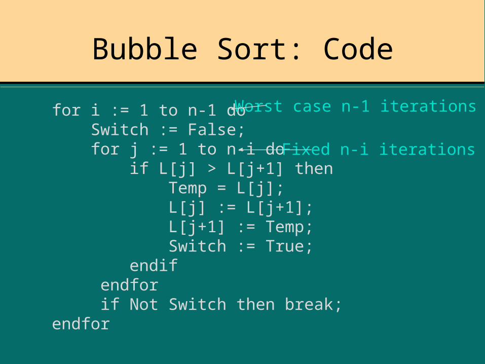
Bubble Sort: Code

for i := 1 to n-1 do Switch := False; for j := 1 to n-i do if L[j] > L[j+1] then Temp = L[j]; L[j] := L[j+1]; L[j+1] := Temp; Switch := True; endif endfor if Not Switch then break;endfor

Worst case n-1 iterations

Fixed n-i iterations

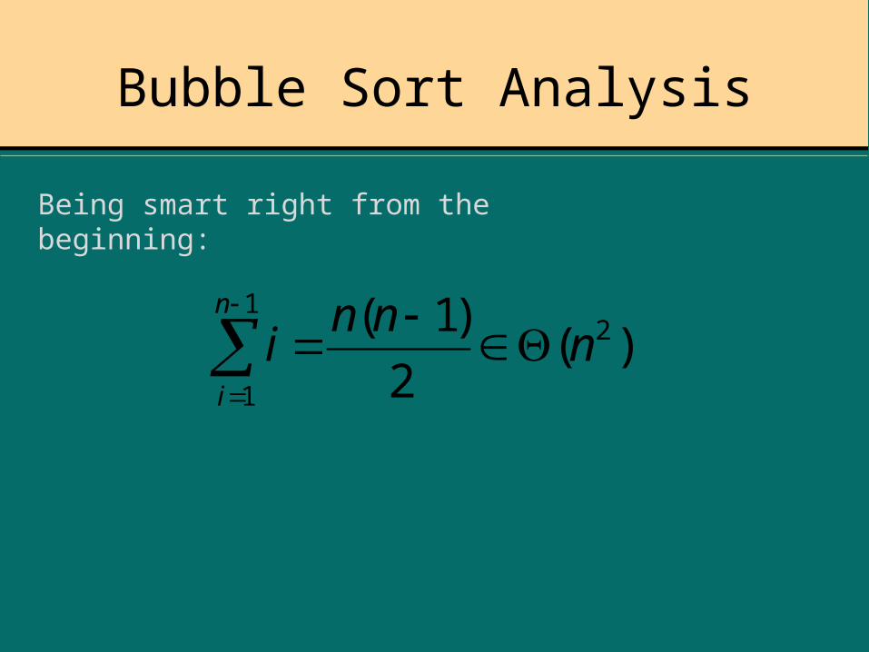
Bubble Sort Analysis

Being smart right from the beginning:

)(2

)1( 21

1

nnn

in

i

Insertion Sort I

• The list is assumed to be broken into a The list is assumed to be broken into a sorted portion and an unsorted portionsorted portion and an unsorted portion

• Keys will be inserted from the unsorted Keys will be inserted from the unsorted portion into the sorted portion.portion into the sorted portion.

Sorted

Unsorted

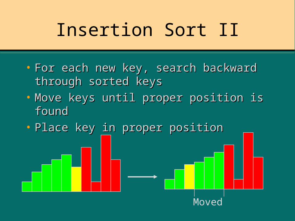
Insertion Sort II

• For each new key, search backward For each new key, search backward through sorted keysthrough sorted keys

• Move keys until proper position is foundMove keys until proper position is found• Place key in proper positionPlace key in proper position

Moved

Insertion Sort: Code

for i:= 2 to n do x := L[i]; j := i-1; while j<0 and x < L[j] do L[j-1] := L[j]; j := j-1; endwhile L[j+1] := x;endfor

Fixed n-1 iterations

Worst case i-1 comparisons

Insertion Sort: Analysis

• Worst Case: Keys are in reverse Worst Case: Keys are in reverse orderorder

• Do i-1 comparisons for each new Do i-1 comparisons for each new key, where i runs from 2 to n.key, where i runs from 2 to n.

• Total Comparisons: 1+2+3+ … + Total Comparisons: 1+2+3+ … + n-1n-1 i

n nn

i

n

1

121

2( )

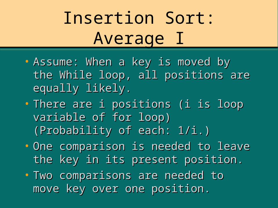
Insertion Sort: Average I

• Assume: When a key is moved by the Assume: When a key is moved by the While loop, all positions are equally While loop, all positions are equally likely.likely.

• There are i positions (i is loop There are i positions (i is loop variable of for loop) (Probability of variable of for loop) (Probability of each: 1/i.)each: 1/i.)

• One comparison is needed to leave One comparison is needed to leave the key in its present position.the key in its present position.

• Two comparisons are needed to Two comparisons are needed to move key over one position.move key over one position.

Insertion Sort Average II

• In general: k comparisons are required In general: k comparisons are required to move the key over k-1 positions.to move the key over k-1 positions.

• Exception: Both first and second Exception: Both first and second positions require i-1 comparisons.positions require i-1 comparisons.

1 2 3 ... ii-1i-2

i-1 i-1 i-2 3 2 1

Position

...

...

Comparisons necessary to place key in this position.

Insertion Sort Average III

1

1

111i

j

ii

ji

Average Comparisons to place one keyAverage Comparisons to place one key

i

i

i

ii

iij

i

i

i

1

2

11

2

2

2

)1(111

1 1

1

SolvingSolving

Insertion Sort Average IV

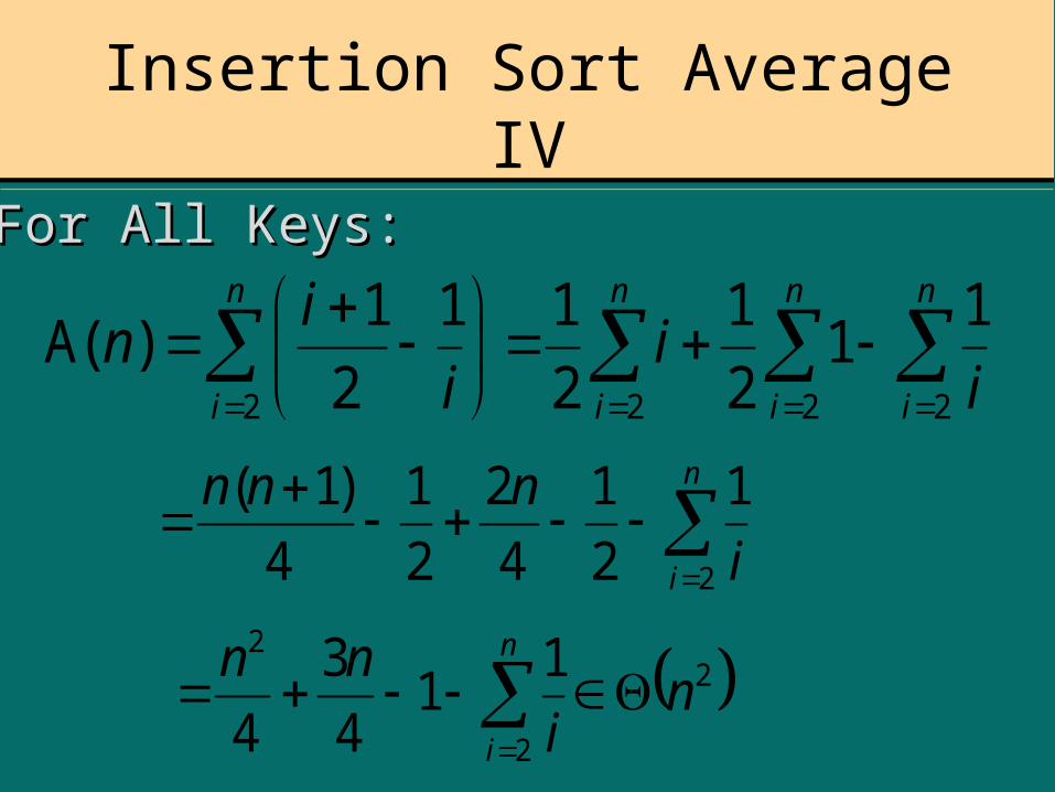
For All Keys:For All Keys:

n

i

n

i

n

i

n

i ii

i

in

2222

11

2

1

2

11

2

1)A(

n

i i

nnn

2

1

2

1

4

2

2

1

4

)1(

2

2

2 11

4

3

4n

i

nn n

i

Optimality Analysis I

• To discover an optimal algorithm we To discover an optimal algorithm we need to find an upper and lower need to find an upper and lower asymptotic bound for a asymptotic bound for a problemproblem..

• An algorithm gives us an upper bound. An algorithm gives us an upper bound. The worst case for sorting cannot The worst case for sorting cannot exceed exceed ((nn22) because we have Insertion ) because we have Insertion Sort that runs that fast.Sort that runs that fast.

• Lower bounds require mathematical Lower bounds require mathematical arguments.arguments.

Optimality Analysis II

• Making mathematical arguments Making mathematical arguments usuallyusually involves assumptions about how the involves assumptions about how the problem will be solved.problem will be solved.

• Invalidating the assumptions invalidates Invalidating the assumptions invalidates the lower bound.the lower bound.

• Sorting an array of numbers requires at Sorting an array of numbers requires at least least ((nn) time, because it would take ) time, because it would take that much time to rearrange a list that that much time to rearrange a list that was rotated one element out of position.was rotated one element out of position.

Rotating One Element

2nd3rd4th

nth1st

2nd3rd

n-1stnth

1stn keys mustbe moved

(n) time

Assumptions:

Keys must be movedone at a time

All key movements takethe same amount of time

The amount of timeneeded to move one keyis not dependent on n.

Other Assumptions

• The only operation used for sorting The only operation used for sorting the list is swapping two keys.the list is swapping two keys.

• Only adjacent keys can be swapped.Only adjacent keys can be swapped.• This is true for Insertion Sort and This is true for Insertion Sort and

Bubble Sort.Bubble Sort.• Is it true for Repeated Minimum? Is it true for Repeated Minimum?

What about if we search the What about if we search the remainder of the list in reverse order?remainder of the list in reverse order?

Inversions

• Suppose we are given a list of Suppose we are given a list of elements L, of size n.elements L, of size n.

• Let i, and j be chosen so 1Let i, and j be chosen so 1i<ji<jn.n.• If L[i]>L[j] then the pair (i,j) is an If L[i]>L[j] then the pair (i,j) is an

inversion.inversion.

1 2 3 45 6 7 8 910

Inversion Inversion Inversion

Not an Inversion

Maximum Inversions

• The total number of pairs is:The total number of pairs is:

• This is the maximum number of This is the maximum number of inversions in any list.inversions in any list.

• Exchanging adjacent pairs of keys Exchanging adjacent pairs of keys removes at most one inversion.removes at most one inversion.

2

)1(

2

nnn

Swapping Adjacent Pairs

Swap Red and Green

The relative position of the Redand blue areas has not changed.No inversions between the red keyand the blue area have been removed.The same is true for the red key andthe orange area. The same analysis canbe done for the green key.

The only inversionthat could be removedis the (possible) onebetween the red andgreen keys.

Lower Bound Argument

• A sorted list has no inversions.A sorted list has no inversions.• A reverse-order list has the maximum A reverse-order list has the maximum

number of inversions, number of inversions, ((nn22) inversions.) inversions.• A sorting algorithm must exchange A sorting algorithm must exchange

((nn22) adjacent pairs to sort a list.) adjacent pairs to sort a list.• A sort algorithm that operates by A sort algorithm that operates by

exchanging adjacent pairs of keys must exchanging adjacent pairs of keys must have a time bound of at least have a time bound of at least ((nn22).).

Lower Bound For Average I

• There are n! ways to rearrange a list of There are n! ways to rearrange a list of n elements.n elements.

• Recall that a rearrangement is called a Recall that a rearrangement is called a permutationpermutation..

• If we reverse a rearranged list, every If we reverse a rearranged list, every pair that used to be an inversion will no pair that used to be an inversion will no longer be an inversion.longer be an inversion.

• By the same token, all non-inversions By the same token, all non-inversions become inversions.become inversions.

Lower Bound For Average II

• There are n(n-1)/2 inversions in a There are n(n-1)/2 inversions in a permutation and its reverse.permutation and its reverse.

• Assuming that all n! permutations are Assuming that all n! permutations are equally likely, there are n(n-1)/4 equally likely, there are n(n-1)/4 inversions in a permutation, on the inversions in a permutation, on the average.average.

• The average performance of a “swap-The average performance of a “swap-adjacent-pairs” sorting algorithm will adjacent-pairs” sorting algorithm will be be ((nn22).).

Quick Sort I

• Split List into “Big” and “Little” keysSplit List into “Big” and “Little” keys

• Put the Little keys first, Big keys secondPut the Little keys first, Big keys second

• Recursively sort the Big and Little keysRecursively sort the Big and Little keys

Little BigPivot Point

Quicksort II

• Big is defined as “bigger than the Big is defined as “bigger than the pivot point”pivot point”

• Little is defined as “smaller than the Little is defined as “smaller than the pivot point”pivot point”

• The pivot point is chosen “at random”The pivot point is chosen “at random”• Since the list is assumed to be in Since the list is assumed to be in

random order, the first element of the random order, the first element of the list is chosen as the pivot pointlist is chosen as the pivot point

Quicksort Split: Code

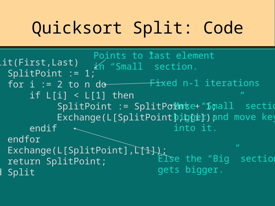
Split(First,Last) SplitPoint := 1; for i := 2 to n do if L[i] < L[1] then SplitPoint := SplitPoint + 1; Exchange(L[SplitPoint],L[i]); endif endfor Exchange(L[SplitPoint],L[1]); return SplitPoint;End Split

Fixed n-1 iterations

Points to last elementin “Small” section.

Else the “Big” sectiongets bigger.

Make “Small” sectionbigger and move keyinto it.

Quicksort III

• Pivot point may not be the exact Pivot point may not be the exact medianmedian

• Finding the precise median is Finding the precise median is hardhard• If we “get lucky”, the following If we “get lucky”, the following

recurrence applies (n/2 is recurrence applies (n/2 is approximate)approximate)

)lg(1)2/(2)( nnnnQnQ

Quicksort IV

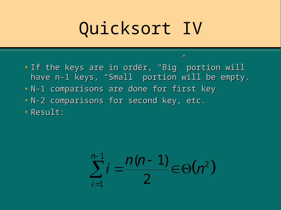
• If the keys are in order, “Big” portion will have n-1 If the keys are in order, “Big” portion will have n-1 keys, “Small” portion will be empty.keys, “Small” portion will be empty.

• N-1 comparisons are done for first keyN-1 comparisons are done for first key• N-2 comparisons for second key, etc.N-2 comparisons for second key, etc.• Result:Result:

in n

ni

n

1

121

2( )

QS Avg. Case: Assumptions

•Average will be taken over Average will be taken over Location of PivotLocation of Pivot

•All Pivot Positions are All Pivot Positions are equally likelyequally likely

•Pivot positions in each call Pivot positions in each call are independent of one are independent of one anotheranother

QS Avg: Formulation

• A(0) = 0A(0) = 0• If the pivot appears at position If the pivot appears at position

i, 1i, 1iin then A(i-1) n then A(i-1) comparisons are done on the comparisons are done on the left hand list and A(n-i) are left hand list and A(n-i) are done on the right hand list.done on the right hand list.

• n-1 comparisons are needed to n-1 comparisons are needed to split the listsplit the list

QS Avg: Recurrence

A n A n n( ) ( ) 1

))1(()1)1(((... nnAnA

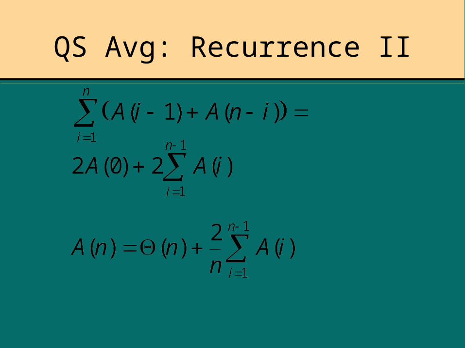
QS Avg: Recurrence II

QS Avg: Solving Recurr.

Guess: A n an n b( ) lg a>0, b>0

( ) lgna

ni i

b

nn

i

n2 21

1

1

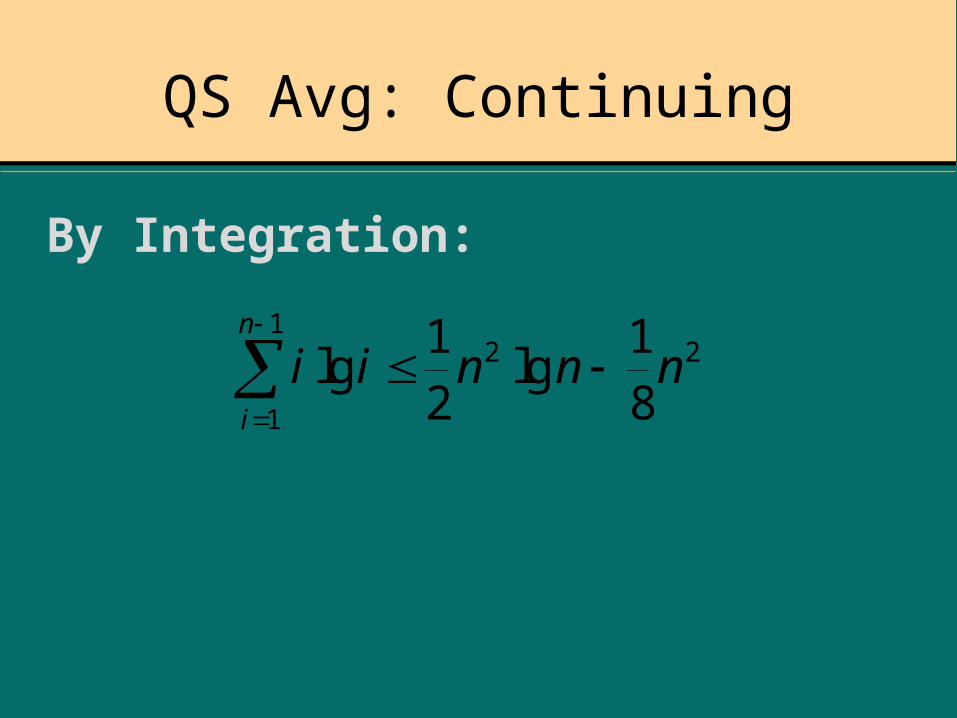
QS Avg: Continuing

By Integration:

i i n n ni

n

lg lg

1

12 21

2

1

8

QS Avg: Finally

an nan b nlg ( )

42

an nan b nlg ( )

42

an n blg

Merge Sort

• If List has only one Element, do If List has only one Element, do nothingnothing

• Otherwise, Split List in HalfOtherwise, Split List in Half

• Recursively Sort Both ListsRecursively Sort Both Lists

• Merge Sorted ListsMerge Sorted Lists

The Merge Algorithm

Assume we are merging lists A and B into list C.

Ax := 1; Bx := 1; Cx := 1;while Ax n and Bx n do if A[Ax] < B[Bx] then C[Cx] := A[Ax]; Ax := Ax + 1; else C[Cx] := B[Bx]; Bx := Bx + 1; endif Cx := Cx + 1;endwhile

while Ax n do C[Cx] := A[Ax]; Ax := Ax + 1; Cx := Cx + 1;endwhilewhile Bx n do C[Cx] := B[Bx]; Bx := Bx + 1; Cx := Cx + 1;endwhile

Merge Sort: Analysis

• Sorting requires no comparisonsSorting requires no comparisons• Merging requires Merging requires nn-1 comparisons in the worst case, -1 comparisons in the worst case,

where where nn is the total size of both lists ( is the total size of both lists (nn key key movements are required in movements are required in allall cases) cases)

• Recurrence relation:Recurrence relation:

W( ) W( / ) lgn n n n n 2 2 1

Merge Sort: Space

• Merging cannot be done in placeMerging cannot be done in place• In the simplest case, a separate list of In the simplest case, a separate list of

size size nn is required for merging is required for merging• It is possible to reduce the size of the It is possible to reduce the size of the

extra space, but it will still be extra space, but it will still be (n)(n)

Heapsort: Heaps

• Geometrically, a heap is an “almost Geometrically, a heap is an “almost complete” binary tree.complete” binary tree.

• Vertices must be added one level at Vertices must be added one level at a time from right to left.a time from right to left.

• Leaves must be on the lowest or Leaves must be on the lowest or second lowest level.second lowest level.

• All vertices, except one must have All vertices, except one must have either zero or two children.either zero or two children.

Heapsort: Heaps II

• If there is a vertex with only one If there is a vertex with only one child, it must be a left child, and child, it must be a left child, and the child must be the rightmost the child must be the rightmost vertex on the lowest level.vertex on the lowest level.

• For a given number of vertices, For a given number of vertices, there is only one legal structurethere is only one legal structure

Heapsort: Heap examples

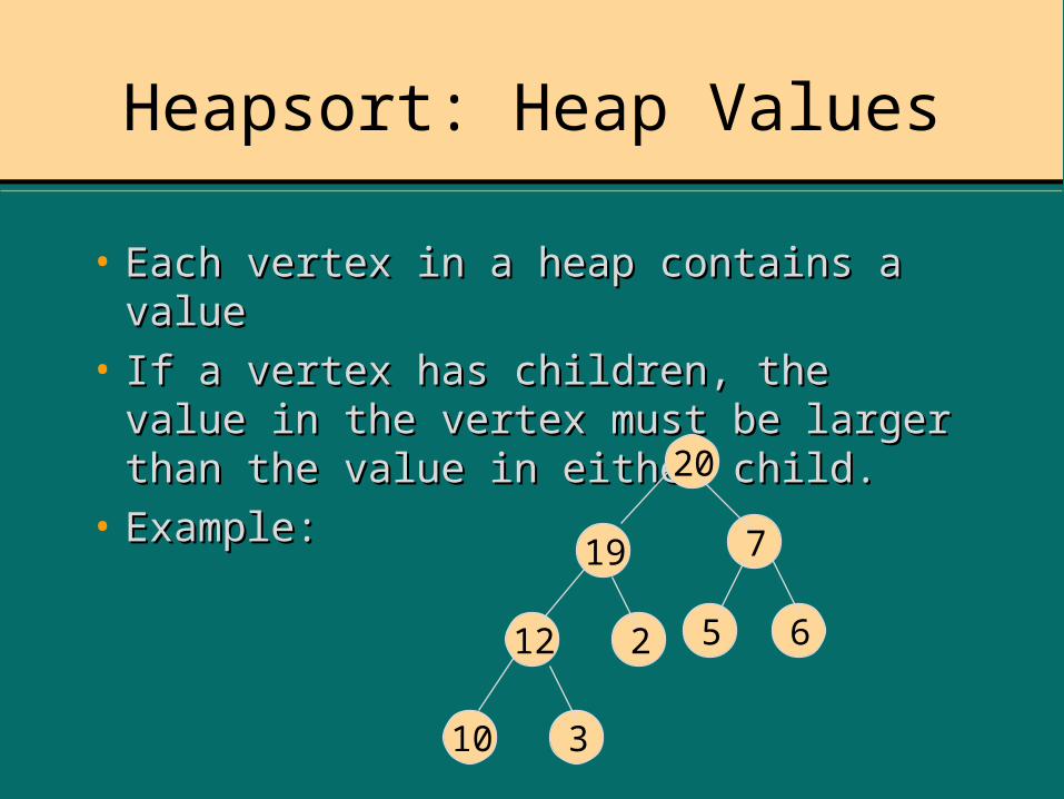
Heapsort: Heap Values

• Each vertex in a heap contains a valueEach vertex in a heap contains a value• If a vertex has children, the value in If a vertex has children, the value in

the vertex must be larger than the the vertex must be larger than the value in either child.value in either child.

• Example:Example:20

19 7

12 2 5 6

310

Heapsort: Heap Properties

• The largest value is in the rootThe largest value is in the root• Any subtree of a heap is itself a heapAny subtree of a heap is itself a heap• A heap can be stored in an array by indexing the vertices thus:A heap can be stored in an array by indexing the vertices thus:• The left child of vertexThe left child of vertex

v has index 2v andv has index 2v andthe right child hasthe right child hasindex 2v+1index 2v+1 1

2 3

4 5 6 7

98

Heapsort: FixHeap

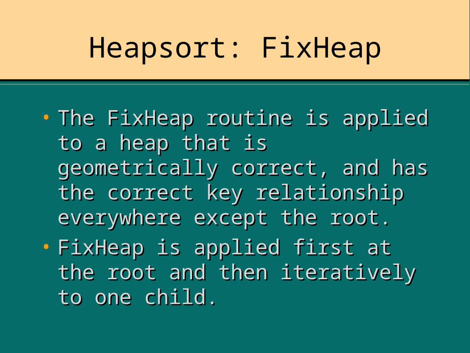
• The FixHeap routine is applied to a The FixHeap routine is applied to a heap that is geometrically correct, heap that is geometrically correct, and has the correct key and has the correct key relationship everywhere except the relationship everywhere except the root.root.

• FixHeap is applied first at the root FixHeap is applied first at the root and then iteratively to one child.and then iteratively to one child.

Heapsort FixHeap Code

FixHeap(StartVertex) v := StartVertex; while 2*v n do LargestChild := 2*v; if 2*v < n then if L[2*v] < L[2*v+1] then LargestChild := 2*v+1; endif endif if L[v] < L[LargestChild] Then Exchange(L[v],L[LargestChild]); v := LargestChild

else v := n; endif endwhileend FixHeap

n is the size of the heap

Worst case run time is(lg n)

Heapsort: Creating a Heap

• An arbitrary list can be turned into a An arbitrary list can be turned into a heap by calling FixHeap on each non-heap by calling FixHeap on each non-leaf in reverse order.leaf in reverse order.

• If n is the size of the heap, the non-leaf If n is the size of the heap, the non-leaf with the highest index has index n/2.with the highest index has index n/2.

• Creating a heap is obviously O(n lg n).Creating a heap is obviously O(n lg n).• A more careful analysis would show a A more careful analysis would show a

true time bound of true time bound of (n)(n)

Heap Sort: Sorting

• Turn List into a HeapTurn List into a Heap

• Swap head of list with last key in Swap head of list with last key in heapheap

• Reduce heap size by oneReduce heap size by one

• Call FixHeap on the rootCall FixHeap on the root

• Repeat for all keys until list is sortedRepeat for all keys until list is sorted

Sorting Example I

20

19 7

12 2 5 6

310

2019 7 12 2 5 6 10 3

19 7

12 2 5 6

3

10

2019 7 12 2 5 6 103

Sorting Example II

19

7

12 2 5 6

3

10

2019 7 12 2 5 6 103

19

712

2 5 63

10

2019 712 2 5 6 103

Sorting Example III

19

712

2 5 6

3

10

2019 712 2 5 610 3

Ready to swap 3 and 19.

Heap Sort: Analysis

• Creating the heap takes Creating the heap takes ((nn) time.) time.• The sort portion is Obviously The sort portion is Obviously ((nnlglgnn))• A more careful analysis would show an A more careful analysis would show an exactexact time bound of time bound of ((nnlglgnn))

• Average and worst case are the sameAverage and worst case are the same• The algorithm runs in placeThe algorithm runs in place

A Better Lower Bound

• The The ((nn22) time bound does not apply ) time bound does not apply to Quicksort, Mergesort, and Heapsort.to Quicksort, Mergesort, and Heapsort.

• A better assumption is that keys can A better assumption is that keys can be moved an arbitrary distance.be moved an arbitrary distance.

• However, we can still assume that the However, we can still assume that the number of key-to-key comparisons is number of key-to-key comparisons is proportional to the run time of the proportional to the run time of the algorithm. algorithm.

Lower Bound Assumptions

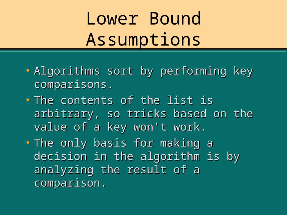
• Algorithms sort by performing key Algorithms sort by performing key comparisons.comparisons.

• The contents of the list is arbitrary, The contents of the list is arbitrary, so tricks based on the value of a so tricks based on the value of a key won’t work.key won’t work.

• The only basis for making a decision The only basis for making a decision in the algorithm is by analyzing the in the algorithm is by analyzing the result of a comparison.result of a comparison.

Lower Bound Assumptions II

• Assume that all keys are distinct, Assume that all keys are distinct, since all sort algorithms must since all sort algorithms must handle this case.handle this case.

• Because there are no “tricks” that Because there are no “tricks” that work, the only information we can work, the only information we can get from a key comparison is:get from a key comparison is:

• Which key is largerWhich key is larger

Lower Bound Assumptions III

• The choice of which key is larger is the only The choice of which key is larger is the only point at which two “runs” of an algorithm point at which two “runs” of an algorithm can exhibit divergent behavior.can exhibit divergent behavior.

• Divergent behavior includes, rearranging Divergent behavior includes, rearranging the keys in two different ways.the keys in two different ways.

Lower Bound Analysis

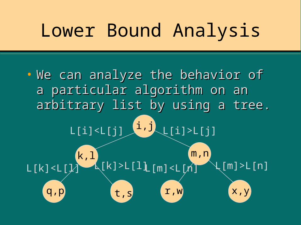
• We can analyze the behavior of a We can analyze the behavior of a particular algorithm on an arbitrary particular algorithm on an arbitrary list by using a tree.list by using a tree.

i,j

k,l m,n

q,p t,s r,w x,y

L[i]<L[j] L[i]>L[j]

L[k]<L[l] L[k]>L[l] L[m]<L[n] L[m]>L[n]

Lower Bound Analysis

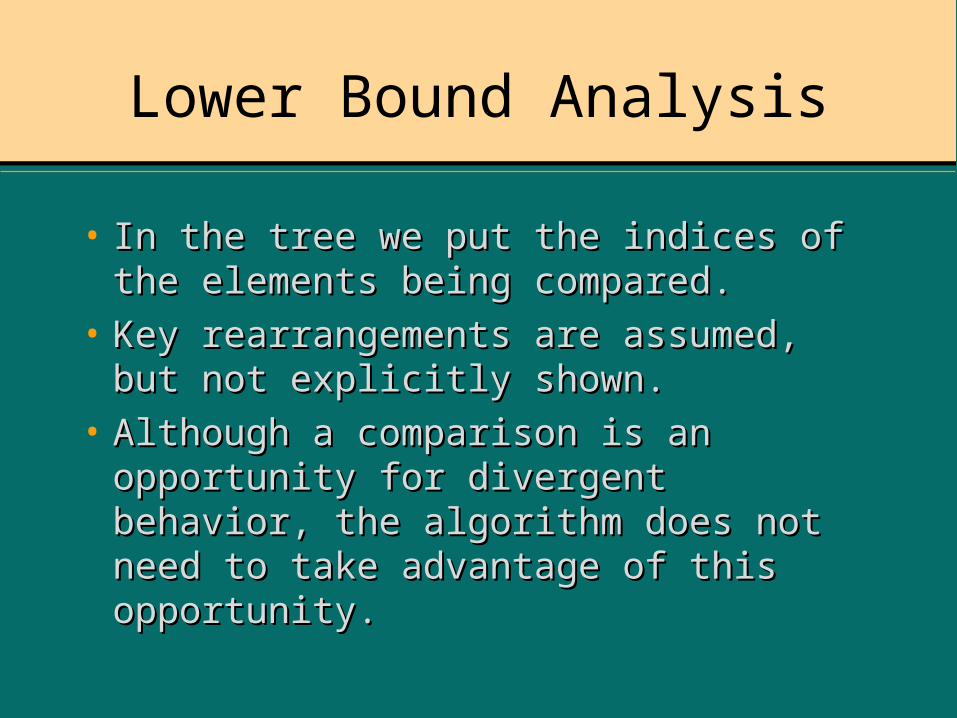
• In the tree we put the indices of In the tree we put the indices of the elements being compared.the elements being compared.

• Key rearrangements are assumed, Key rearrangements are assumed, but not explicitly shown.but not explicitly shown.

• Although a comparison is an Although a comparison is an opportunity for divergent behavior, opportunity for divergent behavior, the algorithm does not need to the algorithm does not need to take advantage of this opportunity.take advantage of this opportunity.

The leaf nodes

• In the leaf nodes, we put a summary In the leaf nodes, we put a summary of all the key rearrangements that of all the key rearrangements that have been done along the path from have been done along the path from root to leaf.root to leaf.

1->22->33->1

2->33->2

1->22->1

The Leaf Nodes II

• Each Leaf node represents a Each Leaf node represents a permutation of the list.permutation of the list.

• Since there are n! initial Since there are n! initial configurations, and one final configurations, and one final configuration, there must be n! configuration, there must be n! ways to reconfigure the input.ways to reconfigure the input.

• There must be at least n! leaf There must be at least n! leaf nodes.nodes.

Lower Bound: More Analysis

• Since we are working on a lower Since we are working on a lower bound, in any tree, we must find the bound, in any tree, we must find the longest path from root to leaf. This is longest path from root to leaf. This is the worst case.the worst case.

• The most efficient algorithm would The most efficient algorithm would minimize the length of the longest minimize the length of the longest path.path.

• This happens when the tree is as close This happens when the tree is as close as possible to a complete binary treeas possible to a complete binary tree

Lower Bound: Final

• A Binary Tree with k leaves must A Binary Tree with k leaves must have height at least lg k.have height at least lg k.

• The height of the tree is the length The height of the tree is the length of the longest path from root to leaf.of the longest path from root to leaf.

• A binary tree with n! leaves must A binary tree with n! leaves must have height at least lg n!have height at least lg n!

Lower Bound: Algebra

n

i

n

i

iin2 2

ln2ln

1lg!lg

n n

i

n

dxxidxx1 2

1

2

lglglg xxxdxx lnln

22ln21)1ln()1(lg1ln2

n

i

nnninnn

)ln(lg)ln(2

nninnn

i

)lg(!lg nnn

Lower Bound Average Case

• Cannot be worse than worst caseCannot be worse than worst case(n lg n)(n lg n)

• Can it be better?Can it be better?• To find average case, add up the To find average case, add up the

lengths of all paths in the decision lengths of all paths in the decision tree, and divide by the number of tree, and divide by the number of leaves.leaves.

Lower Bound Avg. II

• Because all non-leaves have two Because all non-leaves have two children, compressing the tree to children, compressing the tree to make it more balanced will reduce make it more balanced will reduce the total sum of all path lengths.the total sum of all path lengths.

C

X

A B

Switch X and C

C

X

A B

Path from root to C increases by 1,Path from root to A&B decreases by 1,Net reduction of 1 in the total.

Lower Bound Avg. III

• Algorithms with balanced decision trees Algorithms with balanced decision trees perform better, on the average than perform better, on the average than algorithms with unbalanced trees.algorithms with unbalanced trees.

• In a balanced tree with as few leaves In a balanced tree with as few leaves as possible, there will be n! leaves and as possible, there will be n! leaves and the path lengths will all be of length lg the path lengths will all be of length lg n!.n!.

• The average will be lg n!, which isThe average will be lg n!, which is(n lg n)(n lg n)

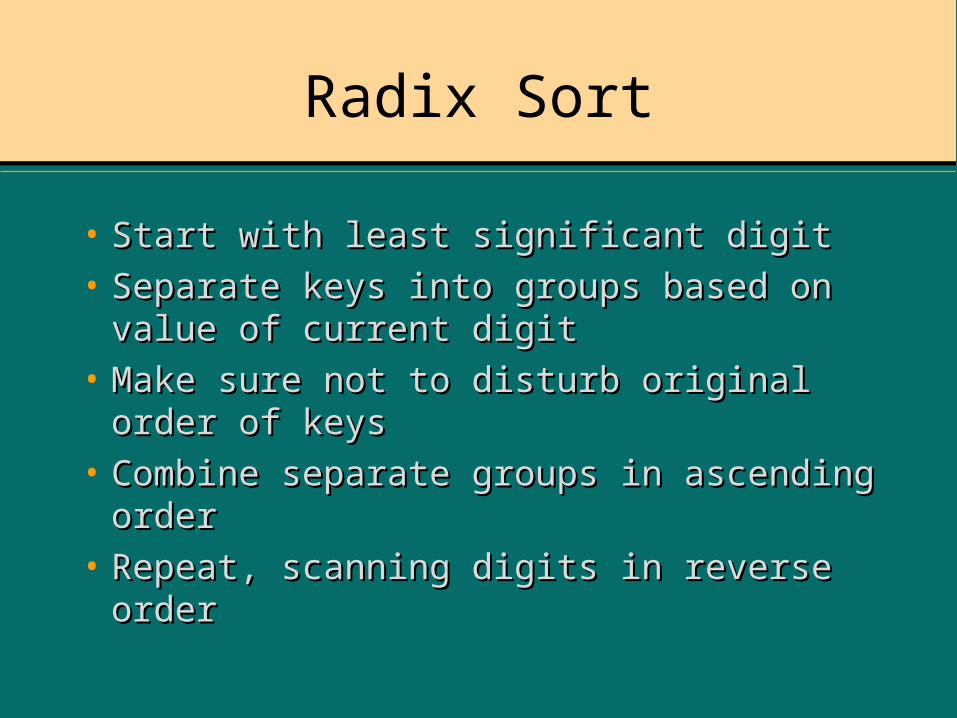
Radix Sort

• Start with least significant digitStart with least significant digit• Separate keys into groups based on Separate keys into groups based on

value of current digitvalue of current digit• Make sure not to disturb original order Make sure not to disturb original order

of keysof keys• Combine separate groups in ascending Combine separate groups in ascending

orderorder• Repeat, scanning digits in reverse orderRepeat, scanning digits in reverse order

Radix Sort: Example

0 0 00 0 1

0 1 00 1 1

1 0 01 0 11 1 0

1 1 1

0 0 0

0 0 1

0 1 0

0 1 1

1 0 0

1 0 1

1 1 0

1 1 1

0 0 0

0 0 1

0 1 0

0 1 1

1 0 0

1 0 1

1 1 0

1 1 1

0 0 0

0 0 1

0 1 0

0 1 1

1 0 0

1 0 1

1 1 0

1 1 1

0 0 0

0 0 10 1 0

0 1 1

1 0 0

1 0 1

1 1 0

1 1 1

0 0 00 0 10 1 00 1 1

1 0 01 0 11 1 01 1 1

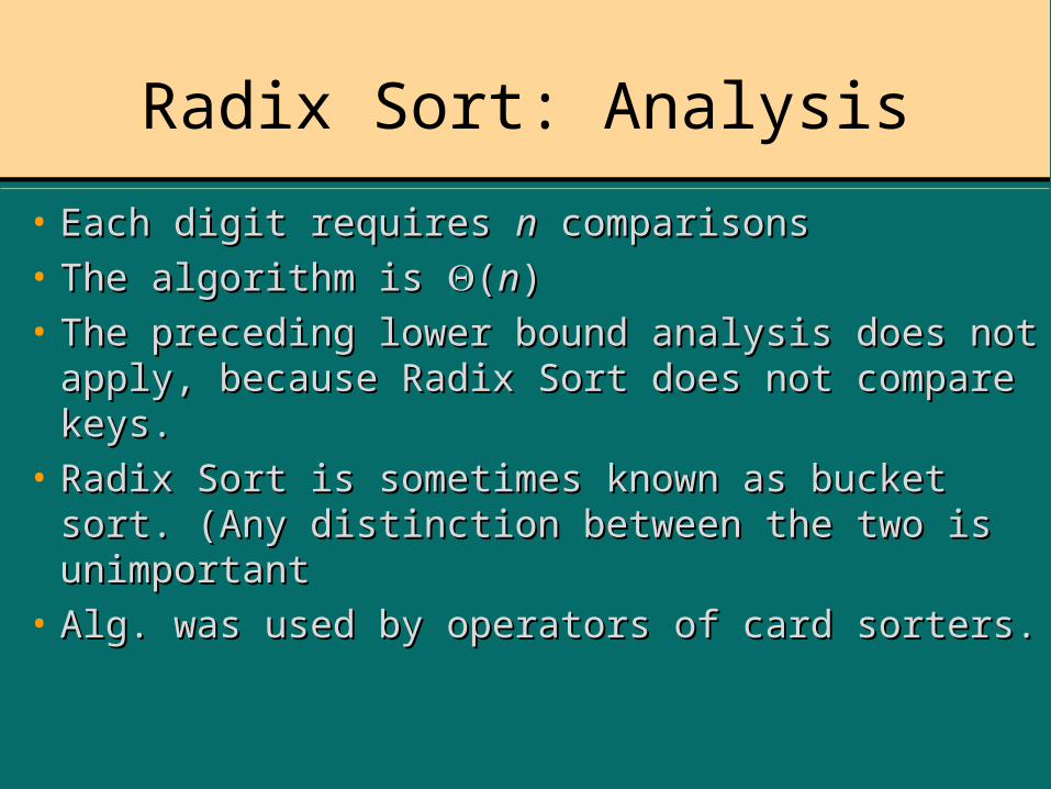
Radix Sort: Analysis

• Each digit requires Each digit requires nn comparisons comparisons• The algorithm is The algorithm is ((nn))• The preceding lower bound analysis does not The preceding lower bound analysis does not

apply, because Radix Sort does not compare apply, because Radix Sort does not compare keys.keys.

• Radix Sort is sometimes known as bucket sort. Radix Sort is sometimes known as bucket sort. (Any distinction between the two is (Any distinction between the two is unimportantunimportant

• Alg. was used by operators of card sorters.Alg. was used by operators of card sorters.