Sonic 2024 Operation Manual · • June 2008 Version 1.1/1.2 • July 2008 Version 1.3 • Aug/Sep 2008 Version 1.4 • December 2008 Version 1.5 • June 2009 Version 1.6

SONIC 2024/2022 BROADBAND MULTIBEAM ECHOSOUNDERS

Operation Manual V5.0 Revision 001 (15May2014)

Part No. 96000001

Page 2 of 210 Version 5.0 Rev r001 Date 15-05-2014 Part No. 96000001

COPYRIGHT NOTICE

Copyright © 2008, R2Sonic LLC. All rights reserved

Ownership of copyright

The copyright in this manual and the material in this manual (including without limitation the text, artwork, photographs, images, or any other material in this manual) is owned by R2Sonic LLC. The copyright includes both the print and electronic version of this manual.

Copyright license

R2Sonic LLC is solely responsible for the content of this manual. Neither this manual, nor any part of this manual, may be copied, translated, distributed or modified in any manner without the express written approval of R2Sonic LLC.

Permissions

You may request permission to use the copyright materials in this manual by writing to [email protected]

Authorship

This manual (Sonic 2024/2022 Operation Manual), and all of the content therein, written by:

R2Sonic LLC

5307 Industrial Oaks Blvd, Suite 120

Austin, Texas 78735

USA

Telephone: +1 (512) 891.0000

Version Printing History

• June 2008 Version 1.1/1.2 • July 2008 Version 1.3 • Aug/Sep 2008 Version 1.4 • December 2008 Version 1.5 • June 2009 Version 1.6 • April 2010 Version 2.0 • August 2010 Version 3.0 • April 2011 Version 3.1 • January 2012 Version 4.0 • April 2012 Version 4.1 • February 2014 Version 5.0

R2Sonic LLC reserves the right to amend or edit this manual at any time. R2Sonic LLC offers no implied warranty concerning the information in this manual. R2Sonic LLC shall not be held liable for any errors within the manual.

Page 3 of 210 Version 5.0 Rev r001 Date 15-05-2014


Table of Contents

1 INTRODUCTION .................................................................................................................. 19

1.1 Outline of Equipment ............................................................................................................ 19

1.2 How to use this Manual ........................................................................................................ 20

1.2.1 Standard of Measurement ........................................................................................... 20

2 SONIC SPECIFICATIONS ....................................................................................................... 21

2.1 Sonic 2024 System Specification ........................................................................................... 21

2.2 Sonic 2022 System Specification ........................................................................................... 21

2.3 Sonic 2024 Dimensions and Weights .................................................................................... 21

2.4 Sonic 2022 Dimensions and Weights .................................................................................... 22

2.5 Sonic 2024/Sonic 2022 Electrical Interface ........................................................................... 22

2.6 Sonic 2024/2022 Ping Rates (SV = 1500.00m/sec) ............................................................... 22

2.7 Acoustic Centre ..................................................................................................................... 23

3 SONIC 2024/2022 SONAR HEAD INSTALLATION – Surface Vessel .......................................... 25

3.1 Sonic 2024/2022 Receive Module Installation ..................................................................... 25

3.1.1 Mounting the Sonic 2024/2022 Receive Module ......................................................... 26

3.1.2 Receive Module ............................................................................................................ 26

3.1.3 Mounting the Projector ................................................................................................ 27

3.1.4 Correct Orientation of the Sonic 2024 and Sonic 2022 ................................................ 29

3.1.5 Deck Test Prior to Deployment .................................................................................... 29

3.2 Sonar Head Installation Guidelines ...................................................................................... 31

3.2.1 Introduction .................................................................................................................. 31

3.2.2 Over-the-Side mount .................................................................................................... 31

3.2.3 Moon Pool Mount ........................................................................................................ 32

3.2.4 Hull Mount .................................................................................................................... 32

3.2.5 ROV Mounting .............................................................................................................. 32

4 SONIC 2024/2022 SONAR INTERFACE MODULE (SIM) INSTALLATION and INTERFACING........ 33

4.1 Sonar Interface Module (SIM) .............................................................................................. 33

4.1.1 Physical installation ...................................................................................................... 33

4.1.2 Electrical and Interfacing .............................................................................................. 34

4.1.3 Serial Communication .................................................................................................. 38


4.1.4 Time and PPS input ....................................................................................................... 38

4.1.5 Motion Input ................................................................................................................. 39

4.1.6 SVP input ....................................................................................................................... 39

5 OPERATION OF THE SONIC 2024/2022 VIA SONIC CONTROL ................................................ 41

5.1 Installing Sonic Control Graphical User Interface ................................................................. 41

5.2 Hot Keys ................................................................................................................................ 41

5.3 Network Setup ....................................................................................................................... 42

5.3.1 Initial Computer setup for Communication .................................................................. 42

5.3.2 Discover Function .......................................................................................................... 43

5.3.3 Configuring Network Communication .......................................................................... 45

5.4 Sensor Setup (Serial and Ethernet Interfacing) ..................................................................... 47

5.4.1 GPS ................................................................................................................................ 47

5.4.2 Motion ........................................................................................................................... 47

5.4.3 Heading ......................................................................................................................... 47

5.4.4 SVP ................................................................................................................................ 48

5.4.5 Message displays .......................................................................................................... 48

5.4.6 Trigger in / Trigger out .................................................................................................. 48

5.5 Sonar Settings (Hotkey: F2) ................................................................................................... 49

5.5.1 Frequency (kHz) ............................................................................................................ 50

5.5.2 Ping Rate Limit .............................................................................................................. 51

5.5.3 Sector Coverage ............................................................................................................ 51

5.5.4 Sector Rotate ................................................................................................................ 52

5.5.5 Minimum Range Gate (m) ............................................................................................. 53

5.5.6 Bottom Sampling ........................................................................................................... 53

5.5.7 Mission Mode ............................................................................................................... 54

5.5.8 IMAGERY ....................................................................................................................... 55

5.5.9 Roll Stabilize .................................................................................................................. 57

5.5.10 Dual Head Mode (Also see Appendix VII, Section 13.9) ............................................... 58

5.5.11 TruePix™, Snippets, Water Column Enable and Intensity Enable ................................. 60


5.6 Ocean Setting ....................................................................................................................... 61

5.6.1 Absorption: 0 – 200 dB/km .......................................................................................... 61

5.6.2 Spreading Loss: 0 – 60 dB ............................................................................................. 61

5.6.3 Time Variable Gain ....................................................................................................... 62

5.7 Installation Settings .............................................................................................................. 65

5.7.1 Projector Orientation ................................................................................................... 65

5.7.2 Projector Z Offset (m) ................................................................................................... 65

5.7.3 Head Tilt........................................................................................................................ 65

5.8 Status .................................................................................................................................... 66

5.9 Tools | Firmware Update...................................................................................................... 69

5.9.1 Firewall and Virus Checker Issues ................................................................................. 71

5.10 Help ....................................................................................................................................... 71

5.10.1 Help Topics ................................................................................................................... 71

5.10.2 Options ......................................................................................................................... 71

5.10.3 Remote Assistance ....................................................................................................... 72

5.10.4 About Sonic Control ...................................................................................................... 72

5.11 Display settings ..................................................................................................................... 73

5.12 Imagery ................................................................................................................................. 74

5.12.1 TruePix™ and Water Column ........................................................................................ 74

5.13 Main Operation Parameters ................................................................................................. 75

5.13.1 Range: 0 – 1200 metres ................................................................................................ 75

5.13.2 RangeTrac™ – Sonic Control automatically sets correct range .................................... 77

5.13.3 Power: 191 – 221 dB ..................................................................................................... 77

5.13.4 Pulse Length: 15µsec – 1000µsec ................................................................................. 77

5.13.5 Gain: 1 – 45 ................................................................................................................... 78

5.13.6 Depth Gates: GateTrac™ .............................................................................................. 78

5.14 Ruler ...................................................................................................................................... 81

5.15 Save Settings ......................................................................................................................... 82

5.16 Operating Sonic Control on a second computer ................................................................... 82

5.16.1 Two computer setup .................................................................................................... 82

5.16.2 Changing back to one computer .................................................................................. 83


6 SONIC 2024/2022 THEORY OF OPERATION .......................................................................... 85

6.1 Sonic 2024/2022 Sonar Head Block Diagram ....................................................................... 85

6.2 Sonic 2024/2022 Transmit (Normal Operation Mode) ......................................................... 86

6.3 Sonic 2024/2022 Receive (Normal Operation Mode) ........................................................... 87

6.4 Sonic 2024/2022 Sonar Interface Module (SIM) Block Diagram ........................................... 89

6.4.1 Sonar Interface Module (SIM) Block Diagram............................................................... 89

7 Appendix I: R2Sonic I2NS Components and Operation ......................................................... 91

7.1 Components .......................................................................................................................... 91

7.2 Connection diagram .............................................................................................................. 92

7.3 Installation ............................................................................................................................ 93

7.3.1 The IMU and GPS antennas .......................................................................................... 93

7.3.2 INS BNC – TNC Connections .......................................................................................... 93

7.3.3 I2NS DB9 Connections ................................................................................................... 94

7.4 Setup in Sonic Control ........................................................................................................... 95

7.4.1 Network Setup .............................................................................................................. 95

7.4.2 Applanix Group 119 specific to R2Sonic SIMINS ........................................................... 96

7.4.3 Sensor Setup ................................................................................................................. 97

7.4.4 INS Monitor (Alt+I) ........................................................................................................ 97

7.5 Measuring IMU Offsets ......................................................................................................... 99

7.6 I2NS Physical Specifications ................................................................................................ 101

7.7 I2NS Drawings ..................................................................................................................... 103

7.7.1 I2NS IMU ..................................................................................................................... 103

7.7.2 I2NS Sonar Interface Module (SIM) ............................................................................ 104

8 APPENDIX II: Multibeam Survey Suite Components ........................................................... 105

8.1 Auxiliary Sensors and Components ..................................................................................... 105

8.2 Differential Global Positioning System ................................................................................ 105

8.2.1 Installation .................................................................................................................. 105

8.2.2 GPS Calibration............................................................................................................ 106

8.3 Gyrocompass ....................................................................................................................... 107

8.3.1 Gyrocompass Calibration Methods ............................................................................. 107

8.4 The Motion Sensor .............................................................................................................. 112


8.5 Sound Velocity Probes ........................................................................................................ 113

8.5.1 CTD Probes ................................................................................................................. 114

8.5.2 Time of Flight Probe ................................................................................................... 115

8.5.3 XBT Probes .................................................................................................................. 115

8.6 The sound velocity cast ....................................................................................................... 116

8.6.1 Time of Day ................................................................................................................. 116

8.6.2 Fresh water influx ....................................................................................................... 116

8.6.3 Water Depth ............................................................................................................... 116

8.6.4 Distance ...................................................................................................................... 116

8.6.5 Deploying and recovering the Sound Velocity Probe ................................................. 116

9 APPENDIX III: Multibeam Surveying .................................................................................. 119

9.1 Introduction ........................................................................................................................ 119

9.2 Survey Design ..................................................................................................................... 119

9.2.1 Line Spacing ................................................................................................................ 119

9.2.2 Line Direction .............................................................................................................. 119

9.2.3 Line Run-in .................................................................................................................. 120

9.3 Record Keeping ................................................................................................................... 120

9.3.1 Vessel Record ............................................................................................................. 120

9.3.2 Daily Survey Log .......................................................................................................... 121

10 APPENDIX IV: Offset Measurements .................................................................................. 125

10.1 Lever Arm Measurement – Offsets ..................................................................................... 125

10.2 Vessel Reference System .................................................................................................... 125

10.3 Measuring Offsets .............................................................................................................. 126

10.3.1 Sonic 2024 Acoustic Centre ........................................................................................ 126

10.3.2 Horizontal Measurement ........................................................................................... 126

10.3.3 Vertical Measurement ................................................................................................ 127

11 APPENDIX V: The Patch Test.............................................................................................. 129

11.1 Introduction ........................................................................................................................ 129

11.2 Orientation of the Sonic 2024/2022 Sonar Head ............................................................... 129

11.3 Patch Test Criteria .............................................................................................................. 130

11.3.1 Latency Test ................................................................................................................ 130


11.3.2 Roll Test ....................................................................................................................... 131

11.3.3 Pitch Test ..................................................................................................................... 132

11.3.4 Yaw Test ...................................................................................................................... 133

11.4 Solving for the Patch Test.................................................................................................... 134

11.5 History ................................................................................................................................. 134

11.6 Basic data collection criteria ............................................................................................... 135

11.7 Patch Test data collection error areas ............................................................................... 135

11.7.1 Positioning .................................................................................................................. 135

11.7.2 Feature chosen for test .............................................................................................. 135

11.7.3 Water depth ............................................................................................................... 136

11.7.4 Use predefined survey lines ....................................................................................... 136

11.7.5 Speed .......................................................................................................................... 136

11.7.6 Vessel line up .............................................................................................................. 136

11.7.7 Pole variability............................................................................................................ 136

11.8 Improving the Patch Test and Patch Test results .............................................................. 137

11.8.1 Need to collect sufficient data ................................................................................... 137

11.8.2 Individually solving values .......................................................................................... 138

11.9 Truthing the patch test ....................................................................................................... 138

12 APPENDIX VI: Basic Acoustic Theory .................................................................................. 139

12.1 Introduction ......................................................................................................................... 139

12.2 Sound Velocity ..................................................................................................................... 139

12.2.1 Salinity ......................................................................................................................... 141

12.2.2 Temperature ............................................................................................................... 141

12.2.3 Refraction Errors ......................................................................................................... 141

12.3 Transmission Losses ............................................................................................................ 142

12.3.1 Spreading Loss............................................................................................................. 142

12.3.2 Absorption................................................................................................................... 143

12.3.3 Reverberation and Scattering ..................................................................................... 147

13 APPENDIX VII: Sonic 2024/2022 Mounting: Sub-Surface (ROV/AUV) .................................. 149

13.1 Installation Considerations ................................................................................................. 149

13.1.1 Ethernet wiring considerations ................................................................................... 150


13.2 Data Rates .......................................................................................................................... 150

13.3 ROV Installation Examples .................................................................................................. 151

13.4 Power Requirements .......................................................................................................... 153

13.4.1 Common mode noise rejection .................................................................................. 155

13.4.2 SIM Power connections .............................................................................................. 156

13.5 SIM Installation – ROV ........................................................................................................ 157

13.6 SIM Installation – AUV ........................................................................................................ 158

13.7 SIM Board Physical Installation .......................................................................................... 159

13.8 SIM Stack LED Status Indicators ......................................................................................... 159

13.8.1 SIM Board Dimensional Information .......................................................................... 160

13.8.2 SIM Board Images ....................................................................................................... 161

13.9 Dual Sonar Head ................................................................................................................. 163

13.9.1 Dual Head Installation ................................................................................................ 163

13.9.2 Operation.................................................................................................................... 163

14 APPENDIX VIII: R2Sonic Control Commands ....................................................................... 165

14.1 Introduction ........................................................................................................................ 165

14.2 General Notes ..................................................................................................................... 165

14.2.1 Ethernet Port Numbers .............................................................................................. 165

14.2.2 Type Definitions .......................................................................................................... 165

14.2.3 Command Packet Format ........................................................................................... 165

14.3 Head Commands, Binary Format........................................................................................ 166

14.4 SIM Commands, Binary Format .......................................................................................... 169

14.5 GUI Commands, Binary Format .......................................................................................... 170

14.6 Command Examples Sent to the Sonar Head and SIM ....................................................... 171

15 APPENDIX IX: R2Sonic Uplink Data Formats ....................................................................... 173

15.1 Introduction ........................................................................................................................ 173

15.2 General Notes ..................................................................................................................... 173

15.3 Port Numbers ...................................................................................................................... 173

15.4 Type Definitions .................................................................................................................. 173

15.5 Ethernet Data Rates ........................................................................................................... 174

15.6 Bathymetry Packet Format ................................................................................................. 175


15.7 Snippet Format .................................................................................................................... 178

15.8 Water Column (WC) Data Format ....................................................................................... 180

15.9 Acoustic Image (AI) Data Format ........................................................................................ 183

15.10 TruePix™ Data Format ........................................................................................................ 185

15.11 Head Status Format ............................................................................................................ 187

15.12 SIM Status Data Format ...................................................................................................... 189

15.13 Device Status Format .......................................................................................................... 191

15.14 Data Playback Using Bit-Twist ............................................................................................ 193

15.14.1 Introduction ................................................................................................................ 193

15.14.2 Capturing Data ............................................................................................................ 193

15.14.3 Editing Data ................................................................................................................. 194

15.14.4 Data Playback .............................................................................................................. 195

16 APPENDIX X: Drawings ...................................................................................................... 197


List of Figures

Figure 1: Sonic 2024/2022 Block Diagram ............................................................................................ 19 Figure 2: Sonic 2024 Acoustic Centre ................................................................................................... 23 Figure 3: Sonic 2024 Acoustic Centre as Mounted ............................................................................... 23 Figure 4: Sonic 2022 Acoustic Centre ................................................................................................... 24 Figure 5: Sonic 2022 Acoustic Centre as Mounted ............................................................................... 24 Figure 6: Sonic 2024 and Sonic 2022 on the mounting frame ............................................................. 25 Figure 7: Top side of Receive Module .................................................................................................. 26 Figure 8: Receive Module Face ............................................................................................................. 26 Figure 9: Seated connectors (Sonic 2024 on left and Sonic 2022 on right) ........................................ 26 Figure 10: Connector wiggle - back and forth NOT up and down ........................................................ 26 Figure 11: Receive Module with cables connected .............................................................................. 27 Figure 12: Sonic 2024 Projector ........................................................................................................... 27 Figure 13: Position the insulating bushing, then wrap threads with Teflon tape, then secure with flat washer, locking washer and then nut. ................................................................................................. 27 Figure 14: Projector Stand-off .............................................................................................................. 28 Figure 15: Mounting the projector ....................................................................................................... 28 Figure 16: View of the mounted Projector; NB. Connector is facing protective fin ............................. 28 Figure 17: SV Probe mounted in block ................................................................................................. 28 Figure 18: Correct Orientation of the Sonic 2024 and the Sonic 2022 ................................................ 29 Figure 19: Typical over-the-side mount ............................................................................................... 31 Figure 20: Sonar Interface Module (SIM) ............................................................................................. 33 Figure 21: Removal of trim to expose securing holes .......................................................................... 34 Figure 22: SIM Interfacing Physical Connections ................................................................................. 35 Figure 23: SIM Interfacing Guide (from label on top of the SIM) ......................................................... 35 Figure 24: SIM IEC mains connection and deck lead Amphenol connector ......................................... 36 Figure 25: Impulse connector ............................................................................................................... 36 Figure 26: Projector cable configuration .............................................................................................. 37 Figure 27: TTL input/output (PPS and Sync In/Out) schematic ............................................................ 38 Figure 28: Sonic Control Icon on desktop ............................................................................................. 41 Figure 29: Sonic Control 2000 .............................................................................................................. 41 Figure 30: Windows XP Internet Properties ......................................................................................... 42 Figure 31: IP and Subnet mask setup ................................................................................................... 43 Figure 32: Sonic Control Network setup .............................................................................................. 44 Figure 33: Set INS IP ............................................................................................................................. 44 Figure 34: Set IP Time Expired .............................................................................................................. 44 Figure 35: Command prompt-ipconfig/all ............................................................................................ 45 Figure 36: Sensor communication settings .......................................................................................... 47 Figure 37: Trigger In/Out Options ........................................................................................................ 48 Figure 38: Sonar Operation Settings window ....................................................................................... 49


Figure 39: Operating Frequency Selection ........................................................................................... 50 Figure 40: UHR frequency available ..................................................................................................... 50 Figure 41: Ping Rate Limit .................................................................................................................... 51 Figure 42: Sector Coverage .................................................................................................................. 52 Figure 43: Sector Rotate ...................................................................................................................... 52 Figure 44: Bottom Sampling Modes .................................................................................................... 53 Figure 45: Example of going from normal to Quad mode ................................................................... 54 Figure 46: Indication of Bottom Sampling Mode ................................................................................. 54 Figure 47: Normal Mission Mode selections ....................................................................................... 54 Figure 48: Mission Mode with the FLS Option installed ...................................................................... 54 Figure 49: Enable Acoustic Image in the wedge display ...................................................................... 55 Figure 50: FLS Wide mode ................................................................................................................... 56 Figure 51: Imagery palette selection in Display Options ..................................................................... 56 Figure 52: Stealth mode single Ping button ......................................................................................... 56 Figure 53: Roll Stabilize ........................................................................................................................ 57 Figure 54: Dual Head Mode ................................................................................................................. 58 Figure 55: Dual Head Mode active ....................................................................................................... 58 Figure 56: Load Settings menu selection ............................................................................................. 59 Figure 57: Loading an .ini file ............................................................................................................... 59 Figure 58: Default dual head Network settings ................................................................................... 59 Figure 59: TruePix™ image of wreck debris and sea grass .................................................................. 60 Figure 60: Ocean Characteristics ......................................................................................................... 61 Figure 61: TVG Curve Concept ............................................................................................................. 62 Figure 62: The angular acoustic wave front will strike each receive element at a different time ...... 64 Figure 63: Installation Settings............................................................................................................. 65 Figure 64: Status Options ..................................................................................................................... 66 Figure 65: Status Message ................................................................................................................... 66 Figure 66: Real-time Status Window ................................................................................................... 67 Figure 67: Select Tools; Firmware Update ........................................................................................... 69 Figure 68: The Browse button will open the current GUI's directory .................................................. 69 Figure 69: Select correct update .bin file ............................................................................................. 70 Figure 70: A batch file will automatically load the upgrade file .......................................................... 70 Figure 71: The start of a firmware update. A series of dots represents the update progress. .......... 70 Figure 72: Firmware update completed, the window will close automatically and the Update window will show successful completion .......................................................................................................... 70 Figure 73: The Help Menu .................................................................................................................... 71 Figure 74: Installed Options ................................................................................................................. 71 Figure 75: Remote Assistance .............................................................................................................. 72 Figure 76: Remote Assistance window ................................................................................................ 72 Figure 77: About, provides the GUI version ......................................................................................... 72 Figure 78: Display Settings ................................................................................................................... 73


Figure 79: Imagery Settings .................................................................................................................. 74 Figure 80: Operating parameter buttons ............................................................................................. 75 Figure 81: Range setting represented in the wedge display ................................................................ 76 Figure 82: Graphical concept of the Wedge Display ............................................................................ 76 Figure 83: RangeTrac enabled .............................................................................................................. 77 Figure 84: Transmit Pulse ..................................................................................................................... 78 Figure 85: Enable Gates ........................................................................................................................ 78 Figure 86: Manual and GateTrac selections ......................................................................................... 78 Figure 87: Manually adjust the gate slope ........................................................................................... 79 Figure 88: Gate width tolerance toggle ................................................................................................ 79 Figure 89: GateTrac enabled; Gate min and max control is disabled .................................................. 79 Figure 90: GateTrac: Depth + Slope enabled, manual gate controls are disabled. .............................. 80 Figure 91: GateTrac: Depth + Slope enabled and tracking a steep slope............................................. 80 Figure 92: Graphical representation of depth gate .............................................................................. 81 Figure 93: Ruler Function ..................................................................................................................... 81 Figure 94: Change in GUI IP .................................................................................................................. 83 Figure 95: SONIC 2024 Sonar Head Block Diagram .............................................................................. 85 Figure 96: Transmit pattern .................................................................................................................. 86 Figure 97: Receive pattern with Transmit pattern ............................................................................... 87 Figure 98: Sonar Interface Module Block Diagram .............................................................................. 89 Figure 99: R2Sonic I2NS Main Components (not including antennas and cables) ............................... 91 Figure 100: GNSS Antennas .................................................................................................................. 91 Figure 101: INS connections ................................................................................................................. 92 Figure 102: INS SIM block diagram ....................................................................................................... 92 Figure 103: INS BNC & TNC Connections .............................................................................................. 93 Figure 104: PPS Out - PPS In ................................................................................................................. 93 Figure 105: Com 1 and Com 2 on SIMINS for POS MV serial data ....................................................... 94 Figure 106: POSView Serial port setup ................................................................................................. 94 Figure 107: Network Settings SIMINS .................................................................................................. 95 Figure 108: Cannot Change IP, waiting on msg 32 ............................................................................... 95 Figure 109: Set IP time expired, cannot change IP ............................................................................... 95 Figure 110: Sensor setup for SIMINS .................................................................................................... 97 Figure 111: INS Monitor ....................................................................................................................... 97 Figure 112: IMU Reference indicators .................................................................................................. 99 Figure 113: POSView Lever Arm setup ............................................................................................... 100 Figure 114: View of installation with the entered offsets .................................................................. 100 Figure 115: IMU Drawing.................................................................................................................... 103 Figure 116: I2NS SIM Drawing ............................................................................................................ 104 Figure 117: Gyrocompass Calibration method 1 ................................................................................ 109 Figure 118: Gyro Calibration Method 2 .............................................................................................. 110 Figure 119: Gyro Calibration Method 2 example ............................................................................... 111


Figure 120: Idealised concept of Gyro Calibration Method 2 ............................................................ 111 Figure 121: CTD Probe ....................................................................................................................... 114 Figure 122: Time of Flight SV probe ................................................................................................... 115 Figure 123: Deploying a sound velocity probe via a winch or A - Frame ........................................... 118 Figure 124: Rough log, kept during survey operations...does not need to be neat, but must contain all pertinent information ................................................................................................................... 123 Figure 125: Smooth log; information copied from real-time survey log ........................................... 124 Figure 126: Vessel Horizontal and Vertical reference system ........................................................... 126 Figure 127: Sonic 2024/2022 Acoustic Centre ................................................................................... 126 Figure 128: Sonic 2024/2022 axes of rotation ................................................................................... 129 Figure 129: Latency Data collection ................................................................................................... 130 Figure 130: Roll data collection .......................................................................................................... 131 Figure 131: Roll data collections ........................................................................................................ 131 Figure 132: Pitch data collections ...................................................................................................... 132 Figure 133: Yaw data collection ......................................................................................................... 133 Figure 134: In 1822 Daniel Colloden used an underwater bell to calculate the speed of sound under water in Lake Geneva, Switzerland at 1435 m/Sec, which is very close to recent measurements. .. 139 Figure 135: Concept of refraction due to different sound velocities in the water column ............... 140 Figure 136: Sound velocity profile ..................................................................................................... 140 Figure 137: Refraction Error indication .............................................................................................. 141 Figure 138: Concept of Spherical Spreading ...................................................................................... 142 Figure 139: Concept of Cylindrical Spreading .................................................................................... 143 Figure 140: Single Head ROV Installation scheme A .......................................................................... 151 Figure 141: Single Head ROV Installation scheme B (Preferred) ....................................................... 151 Figure 142: Dual Head ROV Installation scheme A ............................................................................ 152 Figure 143: Dual Head ROV Installation scheme B (Preferred) ......................................................... 152 Figure 144: Sonic 2024 power supply current waveform. Peak current is 1.770A at 48V. Sonar settings: pulse width = 100us, Tx Power = 221dB, Freq = 400 kHz. ................................................... 154 Figure 145: Sonic 2022 power supply current waveform. Peak current is 1.340A at 48V. Sonar setting: pulse width = 100us, Tx Power = 221dB, Freq = 400 kHz. .................................................... 154 Figure 146: Inrush current to 2024 head during power up, 20 ms window. ..................................... 154 Figure 147: Inrush current to the 2024 head during power up, 1 second window. .......................... 155 Figure 148: Power supply choke installation on 48VDC power ......................................................... 155 Figure 149: SIM Controller Power Connections ................................................................................. 156 Figure 150: J6 Connector on SIM Controller board ........................................................................... 156 Figure 151: ROV installation block diagram with the SIM top-side ................................................... 157 Figure 152: ROV installation block diagram with the SIM controller board mounted in the vehicle electronics bottle and GPS (ZDA or UTC formats) and PPS signals are supplied by top-side equipment ........................................................................................................................................................... 157


Figure 153: ROV installation block diagram with the SIM controller board mounted in the vehicle electronics bottle. GPS (ZDA or UTC formats) and PPS signals are supplied by the vehicle time system. ............................................................................................................................................... 157 Figure 154: Typical wiring. GPS (ZDA or UTC formats) and PPS signals are supplied by the vehicle time system ........................................................................................................................................ 158 Figure 155: SIM Board Stack ............................................................................................................... 158 Figure 156: SIM Stack height .............................................................................................................. 158 Figure 157: SIM Controller Board installation dimensions................................................................. 160 Figure 158: SIM Stack Outline ............................................................................................................ 160 Figure 159: Assembled SIM Boards .................................................................................................... 161 Figure 160: SIM Boards height ........................................................................................................... 161 Figure 161: Default .ini settings file .................................................................................................... 163 Figure 162: Dual head IP and UDP defaults ........................................................................................ 163 Figure 163: Dual-sonar head ping modes ........................................................................................... 164 Figure 164: Dual Head - Dual SIM external interfacing ...................................................................... 164 Figure 165: Wireshark Capture Options ............................................................................................. 194 Figure 166: Sonic 2024/2022 Projector .............................................................................................. 198 Figure 167: Sonic 2024 Receive Module ............................................................................................ 199 Figure 168: Sonic 2022 Receive Module ............................................................................................ 200 Figure 169: Sonic 2024 Mounting Bracket Drawing 1 ........................................................................ 201 Figure 170: Sonic 2024 Mounting Bracket Drawing 2 ........................................................................ 202 Figure 171: Sonic 2022 Mounting Bracket Drawing 1 ........................................................................ 203 Figure 172: Sonic 2022 Mounting Bracket Drawing 2 ........................................................................ 204 Figure 173: Sonic 2024/2022 Mounting Bracket Flange .................................................................... 205 Figure 174: SIM Box Drawing ............................................................................................................. 206 Figure 175: SIM Stack Outline ............................................................................................................ 207 Figure 176: R2Sonic Deck lead minimum connector passage dimensions ........................................ 208 Figure 177: I2NS IMU Dimensions ...................................................................................................... 209 Figure 178: I2NS SIM Dimensions ....................................................................................................... 210


List of Tables

Table 1: Metric to Imperial conversion table ....................................................................................... 20 Table 2: System Specification .............................................................................................................. 21 Table 3: Component Dimensions and Mass ........................................................................................ 21 Table 4: Electrical Interface ................................................................................................................. 22 Table 5: Ping Rate table ....................................................................................................................... 22 Table 6: Deck Lead Pin Assignment (Gigabit Ethernet and Power) ..................................................... 36 Table 7: DB-9M RS-232 Standard Protocol .......................................................................................... 38 Table 8: SIM DB-9M Serial pin assignment .......................................................................................... 38 Table 9: I2NS Dimensions and Mass .................................................................................................. 101 Table 10: Electrical Specifications ...................................................................................................... 101 Table 11: Gyro Calibration Method 2 computation ........................................................................... 111 Table 12: Absorption Values for Seawater and Freshwater at 400 kHz and 200 kHz........................ 144 Table 13: Operating Frequency - water temperature - absorption ................................................... 146 Table 14: Systems Power Requirements ........................................................................................... 153 Table 15: SIM Gigabit switch speed indicators .................................................................................. 159

List of Graphs

Graph 1: Depth errors due to incorrect roll alignment ..................................................................... 131 Graph 2: Position errors as a result of pitch misalignment; error can be either negative or positive ........................................................................................................................................................... 132 Graph 3: Along track position error caused by 0.5° error in yaw patch test ..................................... 133 Graph 4: Along-track position error caused by 1.0° error in yaw patch test error ............................ 134 Graph 5: Seawater Absorption (Salinity 35ppt) ................................................................................. 145 Graph 6: Freshwater Absorption ....................................................................................................... 145


1 INTRODUCTION

1.1 Outline of Equipment The R2Sonic Sonic 2024 and Sonic 2022 Multibeam Echosounder (MBES) is based on fifth generation Sonar Architecture that networks all of the modules and embeds the processor and controller in the sonar head’s Receive Module to make for a very simple installation. The Sonic Control Graphical User Interface (GUI) is a simple program that can be installed on any Windows based computer and allows the surveyor to control the operating parameters of the Sonic 2024/2022. Sonic Control communicates with the Sonar Interface Module (SIM) via Ethernet. The SIM supplies power to the sonar head, synchronises multiple heads, time tags sensor data, relays commands to the sonar head, and routes the raw multibeam data to the customer’s Data Collection Computer (DCC).

The Sonic 2024 and Sonic 2022 work on a user selectable frequency range of 200 kHz to 400 kHz so it is adaptable to a wide range of survey depths and conditions. The user can adjust the operating frequency, via the Sonic Control GUI, on the fly, without having to shut down the sonar system or change hardware or halt recording data. The Sonic 2024/2022 has a user selectable opening angle, from 10° to 160°, using all 256 beams; the desired opening angle can be selected on the fly without a halt to data recording. The selected swath angle can also be rotated port or starboard, whilst recording, to direct the highly concentrated beams towards the desired target. Both the opening angle and swath rotation can be controlled via the mouse cursor.

Figure 1: Sonic 2024/2022 Block Diagram


1.2 How to use this Manual This manual is designed to cover all aspects of the installation and operation of the Sonic 2024 and Sonic 2022. It is, therefore, recommended that the user read through the entire Operation Manual before commencing the installation or use of the equipment.

1.2.1 Standard of Measurement The Metric system of measurement is utilised throughout this manual; this includes temperature in degrees Celsius.

METRIC IMPERIAL

10mm (0.010m) 0.39 inches

100mm (0.100m) 3.9 inches

1000mm (1.0 metre) 39.4 inches

100 grams (0.100kg) 3.5 ounces

1000 grams (1.0 kilogram) 2.2 pounds

10° C 50°F

Table 1: Metric to Imperial conversion table


2 SONIC SPECIFICATIONS

2.1 Sonic 2024 System Specification System Feature Specification

Frequency 400kHz / 200kHz Beamwidth – Across Track (at nadir) 0.5°@ 400kHz / 1.0° @ 200kHz Beamwidth – Along Track (at nadir) 1.0° @ 400kHz / 2.0° @ 200kHz UHR Beamwidth (at nadir) 0.3° Across Track x 0.6° Along Track Number of Beams 256 Swath Sector 10° to 160° (user selectable) UHR Swath Sector 10° to 60° (user selectable) Maximum Slant Range 1200 metres Pulse Length 15µSec – 1000µSec Pulse Type Shaped Continuous Wave (CW) Depth Rating 100 metres (3000 metres optional) Operating Temperature -10° C to 40° C Storage Temperature -30° C to 55° C Table 2: System Specification

2.2 Sonic 2022 System Specification System Feature Specification

Frequency 400kHz / 200kHz Beamwidth – Across Track (at nadir) 1.0°@ 400kHz / 2.0° @ 200kHz Beamwidth – Along Track (at nadir) 1.0° @ 400kHz / 2.0° @ 200kHz UHR Beamwidth (at nadir) 0.6° Across Track x 0.6° Along Track Number of Beams 256 Swath Sector 10° to 160° (user selectable) UHR Swath Sector 10° to 60° (user selectable) Maximum Slant Range 1200 metres Pulse Length 15µSec – 1000µSec Pulse Type Shaped Continuous Wave (CW) Depth Rating 100 metres (3000 metres optional) Operating Temperature -10° C to 40° C Storage Temperature -30° C to 55° C

2.3 Sonic 2024 Dimensions and Weights Component Dimensions (L x W x D) / Dry Weight

Receiver Module 480mm x 109mm x 190mm / 12.9kg Projector 273mm x 108mm x 86mm / 3.3kg Sonar Interface Module (SIM) 280mm x 170mm x 60mm / 2.4kg I2NS Sonar Interface Module (SIM) 280mm x 170mm x 126.4mm / 4.2kg Receive module and Projector mass in water 5.9kg (Fresh) Table 3: Component Dimensions and Mass


2.4 Sonic 2022 Dimensions and Weights Component Dimensions (L x W x D) / Dry Weight

Receiver Module 276mm x 109mm x 190mm / 7.7kg Projector 273mm x 108mm x 86mm / 3.3kg Sonar Interface Module (SIM) 280mm x 170mm x 60mm / 2.4kg I2NS Sonar Interface Module (SIM) 280mm x 170mm x 126.4mm / 4.2kg Receive module and Projector mass in water 4.0kg (Fresh)

2.5 Sonic 2024/Sonic 2022 Electrical Interface Item Specification

Mains Power 90 – 260 VAC; 45 – 65 Hz Power Consumption (SIM and Sonar Head) 75 Watt (Sonic 2022: 54 Watt) Power Consumption (Sonar Head Only) 50W avg.; 90W Peak (Sonic 2022: 35W avg.; 70W

Peak) Integrated Inertial Navigation System (I2NS) 38.4W (SIM and IMU with Antennas) Uplink/Downlink 10/100/1000Base-T Ethernet Data Interface 10/100/1000Base-T Ethernet Sync IN/OUT TTL GPS Timing 1PPS; RS232 NMEA Auxiliary Sensors RS232 / Ethernet Deck Cable Length 15 metre (optional to 50 metres) Table 4: Electrical Interface

2.6 Sonic 2024/2022 Ping Rates (SV = 1500.00m/sec) RANGE PING RATE

2 - 7 60.0 10 55.4 15 39.4 20 30.6 25 25.0 30 21.1 35 18.3 40 16.1 50 13.0 70 9.4

100 6.7 150 4.5 200 3.4 250 2.7 300 2.3 400 1.7 450 1.5 500 1.4 700 1.0

1000 0.7 1200 0.6

Table 5: Ping Rate table

WARNING THE RECEIVE MODULE IS FILLED WITH OIL THAT WILL FREEZE TO A SOLID AT

-10°C. STORAGE BELOW THIS TEMPERATURE (TO -30°C) IS POSSIBLE IF

THE HEAD IS SLOWLY THAWED OUT PRIOR TO OPERATION.


2.7 Acoustic Centre

Figure 2: Sonic 2024 Acoustic Centre

Figure 3: Sonic 2024 Acoustic Centre as Mounted

Centre of Flange to Alongship offset = 0.182m (0.597ft)

Top of Flange to Z reference = 0.327m (1.073ft)


Figure 4: Sonic 2022 Acoustic Centre

Figure 5: Sonic 2022 Acoustic Centre as Mounted

Centre of Flange to Alongship offset = 0.182m (0.597ft)

Top of Flange to Z reference = 0.327m (1.073ft) Page 24 of 210 Version 5.0 Rev r001 Date 15-05-2014 Part No. 96000001

3 SONIC 2024/2022 SONAR HEAD INSTALLATION – Surface Vessel The Sonic 2024/2022 can be installed on an over-the-side pole, through a moon pool, or as a permanent hull mount. The light weight, small size, and low power consumption makes the Sonic 2024/2022 ideal for underwater vehicle (ROV and AUV) installations.

WARNING DECK LEAD MINIMUM BEND RADIUS =

150MM

3.1 Sonic 2024/2022 Receive Module Installation The Sonic 2024/2022 sonar head is mounted on the standard R2Sonic mounting frame as shown below.

Figure 6: Sonic 2024 and Sonic 2022 on the mounting frame

If the Sonic 2024/2022 sonar head is not pre-mounted, the following guidelines must be followed for proper operation of the system.

• The Receive Module is orientated with the narrow part of the face towards the projector (see above).

• The projector is orientated with the connector towards the end with the protective fin. • The Projector must be mounted with the correct 35mm standoffs in place.


3.1.1 Mounting the Sonic 2024/2022 Receive Module

Figure 7: Top side of Receive Module

Figure 8: Receive Module Face

3.1.2 Receive Module The Receive Module has two connectors; the female connector is for the Projector cable, the male connector is for the deck lead that goes to the SIM. There is a securing ‘ear’ on top of the Receive Module to secure the cables with a cable tie or other similar securing methods. Seat the 0.439m projector cable first. A light spray of silicone lubricant (3M Silicone Lubricant, 3M ID: 62-4678-4930-3) will aid in seating the connectors. Silicone grease is never to be used. The deck lead passes through the hydrophone pole and then through the flange opening. Seat the deck lead after seating the projector cable. ENSURE that all connections are tight with no visible gaps.

Figure 9: Seated connectors (Sonic 2024 on left and Sonic 2022 on right)

Figure 10: Connector wiggle - back and forth NOT up and down

Sonic 2022 Sonic 2024


When inserting or removing the connector, use a left to right or back and forth movement and never an up and down movement.


Figure 11: Receive Module with cables connected

Prior to mounting the Receive Module, the block that holds the sound velocity probe must be secured through the underside of the mounting bracket. Next, mount the Receive Module in the mounting frame. This can be most easily done by putting the receive module face on a piece of cardboard or other material and then lowing the mounting frame down with the threaded bolts passing through the mounting frame. The threads, of the securing bolts, after passing through the frame, must be wrapped with 2 wraps of Teflon™ tape. This is to prevent galling where the nut will freeze on the bolt. Do not tighten beyond 17Newton metre (150 pound-inch or 12.5 pound-foot).

Figure 13: Position the insulating bushing, then wrap threads with Teflon tape, then secure with flat washer, locking washer and then nut.

3.1.3 Mounting the Projector The projector is secured to the frame with two, 35mm stand offs. The stand-offs allow room for the Projector to Receive Module cable to be run. A 6mm drive hex screw secures the projector through the stand-off. The Projector’s connector faces towards the protection fin. Connect the 0.439m interconnect cable’s female end to the Projector’s male bulk head connector. When the connectors are mated, there should be no visible gap between them. A very light spray of silicon lubricant will aid seating the connector.

Figure 12: Sonic 2024 Projector


SV Probe block is secured, via screws, though the underside of the mounting frame


Figure 14: Projector Stand-off

Figure 15: Mounting the projector

Figure 16: View of the mounted Projector; NB. Connector is facing protective fin

Figure 17: SV Probe mounted in block

Sonic 2024

Sonic 2022


3.1.4 Correct Orientation of the Sonic 2024 and Sonic 2022 The Sonic 2024/2022 is designed to be installed with the projector facing forward, or towards the bow. However, if the installation requires the projector to face aft, in Sonic Control, the user can select the orientation to projector aft and this will re-orientate the data output to reflect the projector orientation.

Figure 18: Correct Orientation of the Sonic 2024 and the Sonic 2022

3.1.5 Deck Test Prior to Deployment It is highly recommended that the operation of the sonar be verified prior to putting the sonar or vessel into the water. The deck test will test both the receiver and the transmitter.

3.1.5.1 Communications test The first test is to ensure that computer, running Sonic Control, can communicate with both the sonar head and the SIM.

• Make sure that Sonic Control is installed in the root directory on the computer and not under ProgramFiles nor on the desktop

• Make sure all firewalls are off • Make sure all virus checkers are disabled • Verify the IP4 configuration for the network card being used for the sonar • Make sure that the files, in the Sonic Control directory, are not Read-only, or otherwise

protected by the operating system

3.1.5.2 Receiver rub test This tests the receiver and the receive elements

• Turn transmit power off by positioning the cursor over the Power button, then Shift + left mouse button; this will set transmit power to 0

• Reduce the range • Turn Acoustic Imagery on (under Settings | Displays) • Increase Gain to 30


• Have someone rub the receiver face, slowly, with their hand, along the face of the receiver. Noise will be seen, in the display, that will correspond to the rubbing

• If noise is not seen, try adjusting range or gain • If noise is not seen, check the Impulse connector, on the receiver

3.1.5.3 Transmitter test This tests that the transmitter is transmitting

• Have someone position their ear close to the projector • Set ping rate (Settings | Sonar settings) to 2 Hz • Set pulse width to 100µsecs • Slowly bring up Power • A distinct ‘click’ should be heard at the 2 Hz ping rate • If no clicking is heard, increase pulse width and power • If no clicking is heard, check the projector cable connection • If no clicking is heard, open the Status window and check TX voltage (V); voltage should

increase / decrease with increase / decrease in Power

3.1.5.4 Problems with Deck Test If there are any issues, with the Deck Test, please contact R2Sonic Support immediately. R2Sonic Support can be contacted via email: [email protected]; telephone/SMS: +1.805.259.8142; Skype: chaswbrennan


mailto:[email protected]

3.2 Sonar Head Installation Guidelines

3.2.1 Introduction The proper installation of the Sonic 2024/2022 sonar head is critical to the quality of data that will be realised from the system. No matter the type of installation (hull mount, moon pool, or over-the-side pole); the head must be in an area of laminar flow over the array. Any vibration or movement of the sonar head, independent of vessel motion, will result in reduced swath coverage and noise in the data. To this end, the head must be installed on as sturdy a mounting arrangement as possible; fore and aft guys are NOT recommended as a means to obtain this stability.

The initial investigation of where to mount the sonar head should take into account any engines, pumps, or other mechanical equipment that may not be operating at the time, but may be a cause of vibration or noise when operating under normal survey conditions.

The structural stability of any decks, bulkheads, or superstructure, which will be employed when mounting the sonar head, must be taken into account and strengthened if necessary.

3.2.2 Over-the-Side mount The over-the-side mount is normally employed for shallow water survey vessels and/or temporary survey requirements. The over-the-side mount consists of a frame structure that is attached to the vessel’s hull or superstructure. A pole will be attached to the frame, normally through the use of swivel flanges, flanges, or other means by which the head can be swung up when not in use and deployed when needed. A similar mounting arrangement is the bow – mount, which is specialised form of an over-the-side mount.

In order to ensure stability of the pole, it should have a securing arrangement as close to the water line as possible. As stated above, the use of fore or aft guy wires is strongly discouraged.

When the pole is in the ‘up’ position it should be secured so that there is no or little movement that would be a strain on the flanges or mount. The head should be washed with fresh water as soon as possible and inspected for any damage or marine growth. If the head is to remain in the ‘up’ position; a covering should be put over the head that will protect it from the sun.

Figure 19: Typical over-the-side mount


3.2.3 Moon Pool Mount Deploying the sonar head through a moon pool is usually a more stable mounting arrangement than an over-the-side pole. A moon pool is an area, within a vessel, that is open to the water. The sonar head is normally mounted in such a way that it can be deployed and recovered through the moon pool. The pole or structure that the sonar head is mounted on is normally shorter and sturdier than an over-the-side mount; this can allow for higher survey speeds.

3.2.4 Hull Mount The hull mount is the sturdiest of all possible ways to mount a sonar head. With a hull mount, the sonar head is physically attached to the vessel’s hull. With this way of securing the sonar head, there is no possibility of movement, outside that of the movement of the vessel.

There are disadvantages to the hull mount: the head cannot be inspected easily for marine growth or damage; the vessel may be restricted in the depth of waters that can be surveyed, due to the head being permanently attached to the hull.

A normal hull mount will also involve the fabrication of a fairing, on the hull, to ensure correct flow patterns over the sonar head.

3.2.5 ROV Mounting The Sonic 2024/2022 is ideal for undersea operations due to its compact size and low power consumption. With all processing being done in the Receive Module, all that is required is to provide Ethernet over single mode fibre optic communication, between the SIM and the Receive Module. The 48VDC is supplied via the ROV’s own power distribution.

Please refer to Appendix VII for full details on ROV and AUV installation, interfacing and operation.


4 SONIC 2024/2022 SONAR INTERFACE MODULE (SIM) INSTALLATION and INTERFACING

4.1 Sonar Interface Module (SIM)1

Figure 20: Sonar Interface Module (SIM)

The Sonar Interface Module is the communication centre for the Sonic 2024/2022 multibeam system. The SIM receives commands from Sonic Control 2000 and passes the commands to the sonar head. The SIM also receives the PPS and timing information, which is transferred to the sonar head to accurately time stamp all bathymetry data in the sonar head. The data, from the sonar head, passes through the SIM’s Gigabit switch and onto the data collection computer. Sound velocity, from the probe located near the sonar head, and motion data are also interfaced to the SIM to be passed onto the sonar head.

4.1.1 Physical installation The 15 metre cable, from the Sonic 2024/2022 Receive Module, connects directly to the SIM via an Amphenol ™ style connector. Therefore, the SIM must be located within 15 metres of the sonar head (a 50 metre cable is an option). The SIM is not water or splash proof, so it must be installed in a dry, temperature- controlled environment.

The SIM is small and light enough so as to be unobtrusive, but care needs to be taken that it is secured in such a manner so that it will not fall or move whilst the vessel is at sea. The SIM can be secured to a surface (horizontal or vertical) through the pass-through holes that are under the corner trim pieces. The holes accept: #8-32 pan head, M4 pan head or M5 socket head cap screws. The trim piece can be removed by hand to expose the securing holes.

1 For the I2NS SIM, please refer to Appendix I Page 33 of 210 Version 5.0 Rev r001 Date 15-05-2014

Figure 21: Removal of trim to expose securing holes

4.1.2 Electrical and Interfacing The SIM has four DB-9 male connectors on the front. The label, on the top, clearly shows all connections. Beginning on the left front, the connections are: GPS, Motion, Heading, and Sound Velocity. At present time the GPS time message (for timing), sound velocity, and motion (for roll stabilisation) inputs are enabled. Next to each DB-9 are two vertical LEDs; the top LED responds to the input data: Green – receiving data that is being decoded; Red – no connection; Orange – receiving data that cannot be decoded (wrong baud rate or format setting in the Sonic Control Sensor Settings menu). There is also a LED next to the on/off rocker switch, which is the head connection indicator: Green – head on, Red – head power off or not connected, Orange – problems with communications or if the sonar head current draw is below expected limits.

On the second row up are three BNC connections as well as three Ethernet connections. The BNC, which is above the GPS DB-9, receives the one Pulse Per Second (PPS) from the GPS receiver. The PPS, along with the GPS time information on the DB-9, is used to time stamp and synchronise all data.

The two BNC connections, to the right of the Ethernet connectors, are used to receive and send synchronisation triggers to and from other systems.

Mains voltage (90 – 260VAC) is input via the IEC connector. Above the connector is a rocker switch which turns on the system.

The SIM outputs the bathymetry data (from the sonar head), via the Ethernet, on the Ethernet connection marked DATA (as marked on the label on top of the SIM). All of the RJ45 Ethernet connections are routed to the SIM’s internal Gigabit Ethernet switch.

Pass through holes


Figure 22: SIM Interfacing Physical Connections

Figure 23: SIM Interfacing Guide (from label on top of the SIM)

NB. Again, at the present time, the SIM only takes in the PPS, NMEA Time message, sound velocity (at the sonar head) and motion data, but not heading information.


Figure 24: SIM IEC mains connection and deck lead Amphenol connector

Function Impulse Pin Number

Amphenol MS Pin Number

R2Sonic 10013A Wire Colour

CAT 5

BI_DC+ 4 A Blue Blue BI_DC- 5 B Black paired with Blue Blue/White BI_DB- 7 C Green Green BI_DB+ 8 D Black paired with Green Green/White BI_DD- 11 E Brown Brown BI_DD+ 12 F Black paired with Brown Brown/White BI_DA- 9 G Orange Orange BI_DA+ 10 H Black paired with Orange Orange/White Data Shield 6 n/c Drain Wire Power + 1 J,M Orange, Yellow (#18AWG) Power Return 2 K,L Black, Blue (#18 AWG)

Table 6: Deck Lead Pin Assignment (Gigabit Ethernet and Power)

Figure 25: Impulse connector


Figure 26: Projector cable configuration


4.1.3 Serial Communication All serial interfacing is standard RS-232 protocol.

Pin Data 2 Receive 3 Transmit 5 Ground

Table 7: DB-9M RS-232 Standard Protocol

Pin Data Function 1 Receive2 Secondary Serial Port 2 Receive Primary Serial Input 3 Transmit Primary Serial Output 4 +12VDC +12VDC Power 5 Ground Data and Power Common 6 N/C Not Connected 7 +12VDC +12VDC Power 8 N/C Not Connected 9 Transmit2 Secondary Serial Output

Table 8: SIM DB-9M Serial pin assignment

4.1.4 Time and PPS input

4.1.4.1 Connecting PPS and Time to the SIM In order to provide the most accurate multibeam data possible, the Sonic 2024/2022 takes in the GPS Pulse Per Second (PPS) and NMEA ZDA time message or an ASCII UTC message, which is associated with the pulse, to accurately time stamp the Sonic 2024/2022 data. The data collection software will take in the same PPS and time message to synchronise the computer clock and the auxiliary sensor data.

The PPS is a TTL (transistor – transistor logic) pulse. The SIM box PPS input threshold is ≈ +1.35V with about 0.14V of hysteresis. The PPS input rejects pulses narrower than about a microsecond to reject high frequency cable reflections and ringing, but not all types of noise. The input pulse timing needs to be stable, within about 100ppm, or the SIM box will reject the pulses and the LED will flash red instead of green. The pulse is transmitted to the SIM and the data collection computer via a coaxial cable (such as RG-58); the cable is terminated with BNC connectors so that it is easy to use a ‘T’ adaptor to parallel the PPS to different locations. Connect one end of the coaxial cable to the GPS receiver’s PPS output (via a ‘T’ adaptor, if required) and the other end to the SIM BNC labelled PPS. When a pulse is received, the LED next to the BNC connector will flash green at 1 Hz.

Figure 27: TTL input/output (PPS and Sync In/Out) schematic

D31 provides ESD (electrostatic discharge) protection; it trips at about +/- 35V


The standard time message is a NMEA sentence identified as $GPZDA and is expected to arrive after the PPS. The time message will also, usually, go to the data collection computer, so the ZDA message must either be split or output on two of the GPS receiver’s RS-232 ports.

4.1.4.2 Trimble UTC: UTC yy.mm.dd hh:mm:ss ab<CR><LF>" Trimble GPS receivers provide the PPS time synchronisation message with an ASCII UTC string and not the ZDA string. The SIM expects the UTC to arrive 0.5 seconds before the PPS. When interfacing a Trimble GPS, use the UTC message and not the ZDA for timing information. If both the ZDA and UTC are input, the UTC will take priority; the SIM will automatically ignore ZDA while receiving UTC. The UTC status code (‘ab’) is ignored.

Setting up the time synchronisation is done through the Sonic Control software detailed in Section 5.4.

In that each of the SIM serial ports provides 12VDC on selected pins, it is not recommended to use a fully wired serial interface cable as this may cause some GPS receivers to stop sending data. Use a cable with only pins 2, 3 and 5 wired, if possible.

4.1.5 Motion Input The roll component, of the motion data, is used for roll stabilisation. Supported formats and connection are:

• TSS1 Serial • IXSea TAH Serial or Ethernet UDP ($PHOCT)

It is recommended to set the motion sensor to output the highest baud rate and highest update rate possible, preferably 100 Hz or higher.

Connect the motion data to the DB-9 labelled Motion, on the SIM, or via Ethernet input to one of the RJ45 AUX receptacles. Setting up the serial port or Ethernet parameters is done through Sonic Control, which is covered in Section 5.4.

4.1.6 SVP input

4.1.6.1 Connecting the sound velocity probe The sound velocity probe is used to provide the sound velocity at the sonar head, which is used for the receive beam steering. It is not used for refraction correction; that must be accomplished in the data collection software employing a full water depth sound velocity cast.

4.1.6.2 Valeport miniSVS The miniSVS comes with a 15 metre cable. The cable carries both the DC power (8 – 29V DC) to the probe and the data from the probe to the SIM. The miniSVS is set for a baud rate of 9600 and will start outputting sound velocity (Format: <sp> xxxx.xxx m/sec) as soon as power is applied. The miniSVS cable is terminated with a female DB-9 RS-232 connector; this is attached to the male DB-9


RS-232 connector, on the SIM, marked SVP. The probe is powered through the SIM’s serial port 12VDC supply.

Setting up the SVP input is done through the Sonic Control software detailed in Section 5.4.

4.1.6.3 Other supported sound velocity formats The SIM can also accept sound velocity in the below listed formats. Velocity (V) is parsed out of the messages and all other values are ignored.

SeaBird: "TTT.TTTT,CC.CCCCC,SSSS.SSSS, VVVV.VVV (CR/LF)" (39 chars) SeaBird + P:"TTT.TTTT,CC.CCCCC,PPPPP.PPP,SSSS.SSSS, VVVV.VVV (CR/LF)" (49 chars) SVP-C: "VVVVVDDDDDTTTBBCCCC (CR/LF)" (21 chars) SmartSV: " VVVV.VV (CR/LF)" (11 chars) The last format (“VVVV.VV) is also accepted with a flexible width. There is no setup to accept these other formats, merely set the baud rate and the SIM will automatically parse the sound velocity.


5 OPERATION OF THE SONIC 2024/2022 VIA SONIC CONTROL The Sonic 2024/2022 multibeam echosounders are controlled by the Sonic Control software. The Sonic Control GUI does not require a dedicated computer and is usually installed on the user’s data collection computer.

5.1 Installing Sonic Control Graphical User Interface Sonic Control is supplied on a CD or as an attached file. There is no installation program, merely decompress the program to a folder in a root directory of the computer. Send the R2Sonic.exe to the desktop as a short cut (right click on R2Sonic.exe and choose Send to -> Desktop (create shortcut)). The computer must have the Windows .NET Framework installed. This can be downloaded, for free, from the Microsoft web site (dotnetfix35.exe). NB. Do not install Sonic Control under Windows’ Program Files or put all files on the Desktop.

Figure 28: Sonic Control Icon on desktop

Figure 29: Sonic Control 2000

5.2 Hot Keys • F2 – Brings up the Sonar Settings • Alt+Z – Returns sector to 0 rotation • Alt+X – Takes a snapshot of the GUI • Alt+I – Display INS Monitor


5.3 Network Setup All communication, between the Sonic 2024/2022 and the SIM and data collection computer is via Ethernet. The first step in setting up the sonar system is to establish the correct Ethernet parameters, which include the IP (Internet Protocol), Subnet Mask and UDP (User Datagram Protocol)base port under Settings | Network settings.

5.3.1 Initial Computer setup for Communication Prior to starting Sonic Control 2000 for the first time, the computer’s network parameters must be set correctly to establish the first communication.

Open the computer’s network connections. Identify the NIC (Network Interface Card) that is being used for the Sonic system and select Properties (usually by using the right mouse button context menu, highlight the Internet Protocol (TCP/IP) and select properties. Select ‘Use the following IP address’ and enter:

IP address: 10.0.1.102

Subnet mask: 255.0.0.0

Figure 30: Windows XP Internet Properties

Select Internet Protocol and then select Properties to enter the correct IP and Subnet mask.


Figure 31: IP and Subnet mask setup

5.3.2 Discover Function The sonar head and the SIM have initial IP and UDP ports to establish communication (see below). Communication will not be established until the serial number of sonar head and the SIM are entered in the settings for Sonar 1, in the Sonic Control 2000 Network settings.

Use the Discover function to request the serial number information from all attached R2Sonic equipment. The Discover function will automatically transfer the serial numbers to the correct field.

5.3.2.1 Default Network Configuration Head IP: 10.0.0.86 BasePort: 65500 SIM: 10.0.0.99 BasePort: 65500 GUI: 10.0.1.102 BasePort: 65500 Bathy: 10.0.1.102 BasePort: 4000 (actual port 4000) Snippets: 10.0.1.102 BasePort: 4000 (actual port 4006) TruePix™: 10.0.1.102 BasePort: 4000 (actual port 4001) Water Column: 10.0.1.102 BasePort: 4000 (actual port 4005) INS: 10.0.0.44 No BasePort – Does not apply

It is very important that the exact settings, as shown in Figure 33, are entered. This will allow initial communications to be established with the Sonic system; once communication is established, the IP address can be user configured.

WARNING ALL COMPUTER

FIREWALLS MUST BE DISABLED TO INSURE COMMUNICATION.


Figure 32: Sonic Control Network setup

Until the correct serial numbers are entered, there will be no communication. Once the correct serial numbers are entered, click Apply and dots will be visible in the wedge display signifying communication is established. Using Discover will guarantee that the serial numbers will be entered correctly and verify Ethernet communication between devices.

5.3.2.2 INS Addressing When using the I2NS system, the INS default IP is 10.0.0.44. Initially, the INS will not be ready to receive an IP address. The ‘Set IP’ becomes active when the INS is ready to accept an IP (after one to two minutes). When the time period, to set the IP address is over, the button changes to ‘Set IP Expired’.

Figure 33: Set INS IP

Figure 34: Set IP Time Expired


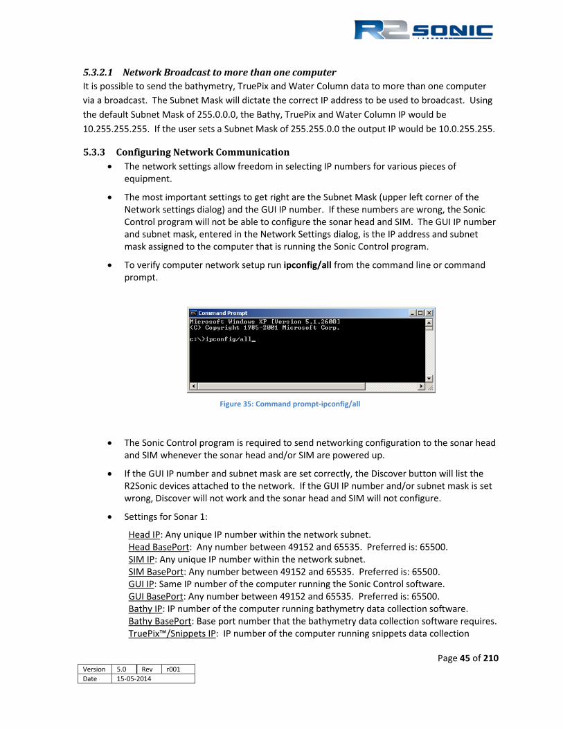
5.3.2.1 Network Broadcast to more than one computer It is possible to send the bathymetry, TruePix and Water Column data to more than one computer via a broadcast. The Subnet Mask will dictate the correct IP address to be used to broadcast. Using the default Subnet Mask of 255.0.0.0, the Bathy, TruePix and Water Column IP would be 10.255.255.255. If the user sets a Subnet Mask of 255.255.0.0 the output IP would be 10.0.255.255.

5.3.3 Configuring Network Communication • The network settings allow freedom in selecting IP numbers for various pieces of

equipment.

• The most important settings to get right are the Subnet Mask (upper left corner of the Network settings dialog) and the GUI IP number. If these numbers are wrong, the Sonic Control program will not be able to configure the sonar head and SIM. The GUI IP number and subnet mask, entered in the Network Settings dialog, is the IP address and subnet mask assigned to the computer that is running the Sonic Control program.

• To verify computer network setup run ipconfig/all from the command line or command prompt.

Figure 35: Command prompt-ipconfig/all

• The Sonic Control program is required to send networking configuration to the sonar head and SIM whenever the sonar head and/or SIM are powered up.

• If the GUI IP number and subnet mask are set correctly, the Discover button will list the R2Sonic devices attached to the network. If the GUI IP number and/or subnet mask is set wrong, Discover will not work and the sonar head and SIM will not configure.

• Settings for Sonar 1:

Head IP: Any unique IP number within the network subnet. Head BasePort: Any number between 49152 and 65535. Preferred is: 65500. SIM IP: Any unique IP number within the network subnet. SIM BasePort: Any number between 49152 and 65535. Preferred is: 65500. GUI IP: Same IP number of the computer running the Sonic Control software. GUI BasePort: Any number between 49152 and 65535. Preferred is: 65500. Bathy IP: IP number of the computer running bathymetry data collection software. Bathy BasePort: Base port number that the bathymetry data collection software requires. TruePix™/Snippets IP: IP number of the computer running snippets data collection


software. TruePix™/Snippets BasePort: Base port number for Snippets, Snippets will be output on a port, which is the base port plus 6. With a base port of 4000, Snippets will be on port 4006; TruePix™ will be on port 4001 Water Column IP: IP address of the computer to receive water column data Water Column BasePort: Base port number for Water Column data; Water Column data will be output on the base port plus 5. The default base port is 4000; Water Column data will be on UDP 4005.

• Settings for Sonar 2: All entries must be zero. Serial numbers are left blank.

• Once networking is set up, Sonic Control will automatically connect upon power up; there is no need to go back into the Network Settings


5.4 Sensor Setup (Serial and Ethernet Interfacing) The Sonar system receives various data, on the SIM serial ports or via the Ethernet. Select Settings | Sensor setting to setup the communications parameters.

Figure 36: Sensor communication settings

5.4.1 GPS The GPS input is for the ZDA time message ($GPZDA) or Trimble UTC message, other NMEA messages may be in the same string; it is not necessary to isolate the ZDA or UTC. In the GPS receiver’s operation manual, there will be an entry that will detail which edge of the PPS pulse is used for synchronisation; this will be either synch on rising edge, or synch on falling edge. Selecting the correct polarity is vital for correct timing.

The firmware supports the ZDA integer part (HHMMSS) and accepts PPS pulses if they pass a basic stability test: the last two pulses must be within 200ppm. If the PPS is unstable or absent, the SIM's internal trained clock-runs with a high degree of accuracy.

The decoded time, from the bathymetry packet, is visible in the main display on the lower left along with the cursor position information. If the displayed time is 01/01/1970 it indicates that timing is not set up correctly.

5.4.2 Motion The motion data is used for roll stabilisation. There are two accepted formats. For serial input, either the TSS1 or the iXSea $PHOCT format is accepted. The iXSea $PHOCT format is also accepted via an Ethernet connection.

The motion data should be at the highest possible baud rate, with the motion sensor configured for the highest output possible; at a minimum 100Hz update.

5.4.3 Heading Not currently enabled.


5.4.4 SVP This is used to set the communication for the sound velocity probe mounted on the sonar head.

5.4.5 Message displays Not currently enabled; see Status Message.

5.4.6 Trigger in / Trigger out Used to receive or send synchronisation TTL pulses. Output goes high when transmitter pings, goes low after receiver has collected data.

Figure 37: Trigger In/Out Options

5.4.6.1 Trigger In • The SIM Synch In input requires a TTL signal (0 to +5V) • The minimum high level trigger point is +2.4V • The trigger pulse width must be longer than 1µsec • The sonar will ping 10.025msecs (±10µsecs) after receiving the trigger

5.4.6.2 Trigger Out • Output is 0 to +5V • If Trigger Out is set to Rising Edge, the output pulse is high during the receive period. If the

Trigger Out is set to Falling Edge the output pulse is low during the receive period.

In the lower portion, of the GUI, the colour indicator will indicate when the Trigger In is active by turning from grey to green . When the Trigger In mode is set to Manual, the colour

indicator will change to yellow . Manual mode allows the sonar to ping every time an external Ethernet command (PNGØ, 1) is received or, if in FLS mode, the Ping button is used.


5.5 Sonar Settings (Hotkey: F2) The Sonic 2024/2022 have many features that provide the user with the versatility to tailor the system to any survey project; many of these features can be controlled either through the Operation Settings or with the mouse cursor.

Figure 38: Sonar Operation Settings window


5.5.1 Frequency (kHz) The Sonic 2024/2022 operates on a user selectable frequency, from 200 kHz to 400 kHz, in 10 kHz steps. The operating frequency can be changed on the fly; there is no need to stop recording data, go offline, or load any firmware. The operating frequency is selected via the drop down menu next to Frequency (kHz).

Figure 39: Operating Frequency Selection

5.5.1.1 700 kHz UHR The optional UHR upgrade enables the sonar to operate at 700 kHz for Ultra High Resolution. If this option is installed, there will be the added 700 kHz frequency, after 400, in the available frequency list. If the upgrade is not installed there will be no listing of this frequency.

Figure 40: UHR frequency available


The UHR upgrade requires a unique projector, which covers the normal 200 – 400 kHz frequency range, but can also provide the necessary power to operate at 700 kHz. The projector is specially labelled with a blue indicator on the end of the projector.

When 700 kHz is selected, the swath sector will automatically be reduced to 60°. The UHR upgrade is intended for short range operation. In the UHR mode of operation, the across track beamwidth is 0.3° and the along track beamwidth is 0.6°: true Ultra High Resolution sonar.

5.5.1.2 UHR Operation Suggestions When operating at the high 700kHz frequency it will be necessary to increase Power and Absorption significantly (Absorption set to 200dB/km). Along with this will be a possible increase in Pulse Length, Gain and Spreading Loss. As frequency increases so does the effect of attenuation and this is why, when in UHR mode, the sonar operating settings need to be increased to increase the total power going into the water and the higher gain needed to receive the attenuated signal. As stated the UHR mode is for short range operation.

5.5.2 Ping Rate Limit The Sonic 2024/2022 can transmit at a rate up to 60 Hz (60 pings per second), this is called the Ping Rate. At times, it may be desirable to reduce the ping rate to reduce the collection software file size or for other reasons. Highlight the box next to Ping Rate Limit and the ping rate limit drop down box will be activated; select a predefined ping rate or enter a manual rate.

Figure 41: Ping Rate Limit

5.5.3 Sector Coverage The Sonic 2024/2022 allows the user to select the swath sector from 10° to 160°. All 256 beams are used, no matter what the selected sector coverage that is chosen. The smaller the sector, the higher the sounding density is within that sector. Changing the Sector Coverage can be done on the fly, with no need to stop recording data or to go offline.


Figure 42: Sector Coverage

5.5.4 Sector Rotate The Sonic 2024/2022 has the capability to direct the selected sector to either port or starboard, allowing the user to map vertical features, or areas of interest, with a high concentration of soundings resulting from the compressed sector.

First, change the sector coverage to the desired opening angle; this will concentrate the 256 beams within the sector, and then increase the Range setting.

Second, rotate the swath towards the feature to be mapped with high definition. This is done on the fly, with no need to stop data recording or to go off line. When rotating, make sure to keep the bottom detections within the confines of the range.

Figure 43: Sector Rotate

The Sector Coverage can also be controlled via the mouse cursor, inside the wedge display.

Position the cursor on either of the straight sides of the wedge; the cursor will change to a double arrow and the sector can be reduced or increased. When using the cursor to change the sector coverage, the change only takes place when the mouse button is released.

The sector angle will be numerically visible in the lower left hand corner of the wedge display while the mouse button is depressed.

The sector can also be rotated using the mouse cursor, in the wedge display. Position the cursor on the curved bottom of the wedge; the cursor will change to a horizontal double arrow, the wedge can now be rotated to port or starboard. The angle of rotation is numerically visible in the lower left hand corner of the wedge display during rotation. A clockwise rotation is positive, an anti-clockwise rotation is negative.

The change only takes place when the mouse button is released. To return to a 0 rotation, use the Hotkey Alt+Z.


5.5.5 Minimum Range Gate (m) This provides a means to block out noise or interference close to the sonar head. Enter the range, in metres, from the sonar head to establish the gate; anything within that range will be blocked. As a safety precaution: This gate should not be used when working in very shallow water.

5.5.6 Bottom Sampling There are two main options: Equiangular or Equidistant. The equiangular and equidistant modes are further enhanced by the Dual/Quad mode, described below. In equidistant mode, all beams are equally distributed, within the sector. There are limits to what the equidistant can do, based on opening angle and bottom topography; it is best on flat sea floor and with an opening angle (Sector Coverage) equal to, or less than, 130°.

Figure 44: Bottom Sampling Modes

5.5.6.1 Dual/Quad Mode The Dual/Quad bottom sampling modes can be used with both equiangular and equidistant sampling. The modes work by spatially distributing the acrosstrack bottom sampling, ping by ping. The beam is slightly repositioned, in the acrosstrack direction, with each ping. This mode was developed for ROV/AUV survey operations.

The Dual/Quad mode will work at all speeds; however, it is at slower speeds, that the Dual or Quad modes will be more evident.

The Dual/Quad mode requires 16-May-2013 head firmware and 17-Oct-2013 GUI or more recent. All firmware from the current, Head$16-may-2013-03-58-29 will have this feature available. All GUIs, from 17Oct2013 and newer will support the Dual/Quad mode.


Figure 45: Example of going from normal to Quad mode

5.5.6.2 Current Mode Display The current Bottom Sampling Mode is shown in the main GUI window, in the lower right, information area.

Figure 46: Indication of Bottom Sampling Mode

The BSM designations:

• ea1 = Equiangular normal • ea2 = Equiangular dual • ea4 = Equiangular quad • ed1 = Equidistant normal • ed2 = Equidistant dual • ed4 = Equidistant quad

5.5.7 Mission Mode The versatility, built into the Sonic 2024/2022, is further enhanced with the ability to adapt the system to the nature of the survey task: normal survey, surveying a vertical feature or the optional Forward Looking Sonar mode.

If the FLS option is not installed, the Mission Mode will only contain the Bathy functions.

Figure 47: Normal Mission Mode selections

Figure 48: Mission Mode with the FLS Option installed


• Down, Bathy Norm: Normal bathymetry survey • Down, Bathy VFeature: With the ability to map vertical surfaces, without physically rotating

the sonar head, this Mission Mode provides improved detection methods tailored to mapping vertical features. This specialised mode greatly reduces the corner ‘ringing’ seen in older technology systems. When using Bathy VFeature, please use Equiangular bottom sampling and not Equidistant.

• Down ,FLS Narrow/Wide: One Forward Looking Sonar mode. No bathymetry output; this setting is for imagery only.

• Up, Bathy Norm; Up, Bathy VFeature: is the same as the above, but orientates the wedge so it is pointing up (used primarily hull inspection type survey).

• Up, FLS Narrow/Wide: Most common setting when using the optional FLS feature

The Mission Mode can be changed on the fly, with no need to stop recording data.

5.5.8 IMAGERY

5.5.8.1 Acoustic Image (Display only) The wedge can display acoustic intensity. This will aid in setting the correct combination of operating parameters (such as power, pulse width and gain). Enabling the Acoustic Intensity will increase the network load.

Enable the wedge Acoustic Intensity under the Display options. The Brightness control, in the main window, is used to set the intensity in the display. A good brightness setting, to start with, is 30dB. Most users also prefer the 1 pixel bathy dot option (on the Display tab), when viewing the Acoustic Image, in the display.

Figure 49: Enable Acoustic Image in the wedge display

5.5.8.2 Forward Looking Sonar Forward looking mode can be in one of two configurations. FLS Wide uses the 20° projector within the standard projector. FLS Narrow uses the 1° standard projector. The wide mode, using the 20° projector, will have a lower source level, but is very good for near field use. The narrow mode allows for full source level to be used (221dB), but is more critical in aiming towards the target due to the 1° transmit pattern.


Figure 50: FLS Wide mode

5.5.8.2.1 FLS Mode adjustments In FLS mode, the Brightness button adjusts the image ‘gain’ up to 80dB. The colour palette is selected in the Display options, under Acoustic Image.

Figure 51: Imagery palette selection in Display Options

The FLS grid visibility is set in the Display | Grid settings. When in FLS mode, the range rings are turned on and off, by the Horizontal Grid Line selection. The angle markers (from nadir) are controlled by the Vertical Grid Line selection.

5.5.8.2.2 Stealth Mode The FLS can be operated in a stealth mode, where the only time the system transmits is when the user manually triggers the sonar using the Ping button. In Sensor Settings, the ‘Trigger In’ option has to be put to Manual (the TRG indicator colour will change to Yellow), simultaneously, the Ping button will appear in the GUI. The only time an image will be updated, is when the user selects the Ping button.

Figure 52: Stealth mode single Ping button


5.5.9 Roll Stabilize When a motion sensor is interfaced to the SIM, the data can be stabilised for the roll motion of the vessel. With the advanced roll stabilisation, in the Sonic 2024/2022, there is no need to stop recording or go off line to change between roll stabilised and non-stabilised mode, nor is there a need to go into the data collection software and identify the data as roll stabilised. The R2Sonic roll stabilisation has been developed based on recommended methods from various data collection software companies.

Roll stabilisation only works within the 160° maximum sector, any swath rotation or large sector size (opening angle) that attempts to go beyond the 160° limit will cause the system to stop roll stabilisation.

As stated in the SIM interfacing, it is recommended that the motion data be at the highest update rate possible.

Figure 53: Roll Stabilize


5.5.10 Dual Head Mode (Also see Appendix VII, Section 13.9) The selections are: Single Head, Simultaneous Ping or Alternating Ping. When the dual head mode is selected, a second wedge display will be available in Sonic Control 2000.

When using dual heads, the sonar heads have to have exactly the same firmware installed. Use the Status display to verify that both heads have the same firmware; if not, update the oldest firmware sonar head to match the most current firmware sonar head.

Figure 54: Dual Head Mode

Figure 55: Dual Head Mode active

In dual head mode, certain controls: Range, Power, Pulse Length, and Gain set both sonar heads.

NB. For a dual head system, the Discover function will only list the systems. Discover does not auto-fill the serial numbers for a dual head system. Correct serial numbers must be entered by hand for both systems.

5.5.10.1 Dual Head default settings To make it easier to set up the system for dual head operation, there is a specific settings file that can be loaded that will set all of the defaults for a dual head configuration. Under the File menu selection, select Load Settings.


Figure 56: Load Settings menu selection

The available settings files will be shown. There are three Factory Default initialisation files; one for single head and two for dual head: dual head – dual SIM or dual head – single SIM.

Figure 57: Loading an .ini file

When the file is loaded, Sonic Control will be configured for dual head mode, this includes the default network settings. If using only one SIM, the second SIM IP and BasePort must be set to zero.

Figure 58: Default dual head Network settings

When only one SIM is used for a dual head system, the Sonar 2 SIM IP and BasePort need to be set to 0. The Serial Number must be left blank. This is the DefaultSettingsDualHead_SingleSIM.ini


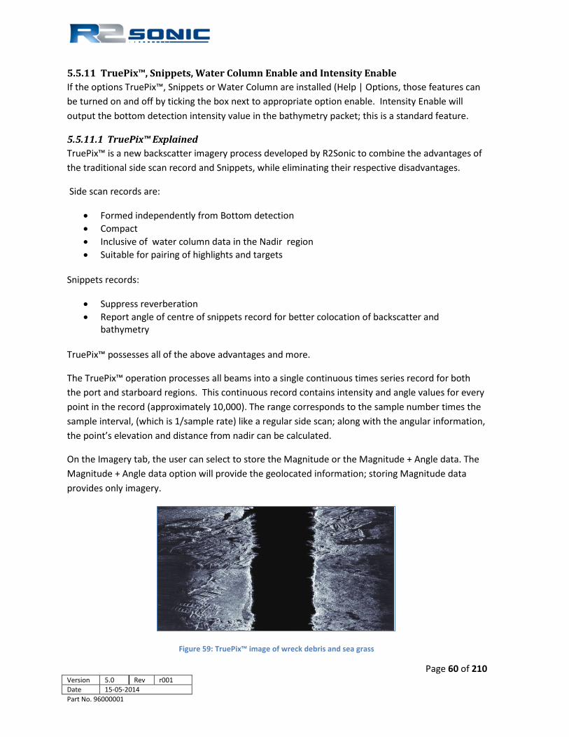
5.5.11 TruePix™, Snippets, Water Column Enable and Intensity Enable If the options TruePix™, Snippets or Water Column are installed (Help | Options, those features can be turned on and off by ticking the box next to appropriate option enable. Intensity Enable will output the bottom detection intensity value in the bathymetry packet; this is a standard feature.

5.5.11.1 TruePix™ Explained TruePix™ is a new backscatter imagery process developed by R2Sonic to combine the advantages of the traditional side scan record and Snippets, while eliminating their respective disadvantages.

Side scan records are:

• Formed independently from Bottom detection • Compact • Inclusive of water column data in the Nadir region • Suitable for pairing of highlights and targets

Snippets records:

• Suppress reverberation • Report angle of centre of snippets record for better colocation of backscatter and

bathymetry

TruePix™ possesses all of the above advantages and more.

The TruePix™ operation processes all beams into a single continuous times series record for both the port and starboard regions. This continuous record contains intensity and angle values for every point in the record (approximately 10,000). The range corresponds to the sample number times the sample interval, (which is 1/sample rate) like a regular side scan; along with the angular information, the point’s elevation and distance from nadir can be calculated.

On the Imagery tab, the user can select to store the Magnitude or the Magnitude + Angle data. The Magnitude + Angle data option will provide the geolocated information; storing Magnitude data provides only imagery.

Figure 59: TruePix™ image of wreck debris and sea grass


5.6 Ocean Setting

Figure 60: Ocean Characteristics

Ocean Characteristics include Absorption and Spreading loss, which are the main components of the Time Variable Gain (TVG) computation, and manual Sound Velocity (for receive beam steering).

5.6.1 Absorption: 0 – 200 dB/km Absorption is influenced primarily by frequency and the chemical compounds of boric acid B(OH)3 and magnesium sulphate MgSO4.

It is highly recommended that the local absorption value be entered. If this is not known, a good on-line source is: http://resource.npl.co.uk/acoustics/techguides/seaabsorption/2

Appendix VI provides a table of absorption values based on operating frequency.

5.6.2 Spreading Loss: 0 – 60 dB Spreading loss is the loss of intensity of a sound wave, due to dispersion of the wave front. It is a geometrical phenomenon and is independent of frequency. The sound wave propagates in a spherical manner, the area of the wave front increases as the square of the distance from the source. Therefore, the sound intensity decreases with the square of the distance from the projector. Spreading loss is not dependent on frequency.

Spreading loss is not a setting that normally needs to be changed except when surveying in deeper depths. As spreading loss is not dependent on frequency, the setting is unaffected by a change in operating frequency. A general default value of 20 – 30 is normally sufficient for most survey conditions. However, the value should be increased when surveying into deeper depths (>100 metres)

NB. In very shallow water (2m or less) it may be more advantageous to use Fixed Gain. To put the system into Fixed Gain enter zero (0) for both Spreading Loss and Absorption.

For more detailed information on absorption and spreading loss, please refer to Appendix VI Basic Acoustic Theory.

2 Linked with the kind permission of the National Physical Laboratory; Teddington, United Kingdom TW11 0LW; NPL reserves the right to amend, edit or remove the linked web page at any time. Page 61 of 210 Version 5.0 Rev r001 Date 15-05-2014

http://resource.npl.co.uk/acoustics/techguides/seaabsorption/

5.6.3 Time Variable Gain Absorption and spreading loss are the main components of the Time Variable Gain (TVG) computation.

TVG Equation

TVG = 2*R* α/1000 + Sp*log(R) + G

α = Absorption Loss db/km R = Range in metres Sp = Spreading loss coefficient G = Gain from Sonar Control setting

TVG is employed in underwater acoustics to compensate for the nature of the reflected acoustic energy. When an acoustic pulse is transmitted in a wide pattern, the first returns will generally be from the nadir region and very strong. As the receive window time lengthens, the weaker returns are received. Using a fixed gain would apply either too much gain for the early returns or insufficient gain for the later returns. The solution is to use TVG. The function of TVG is to increase gain continuously throughout the receive cycle. Therefore, smaller gain corresponds with the first returns (normally the strongest) and higher gain corresponds to the later returns (normally the weakest). This function is represented in, what is called, the TVG curve.

5.6.3.1 TVG Curve The TVG curve can be either shallow or steep depending mostly on the Absorption value to define the shape of the curve. The Spreading Loss will determine the amplitude of the gain.

Figure 61: TVG Curve Concept


5.6.3.2 Sound Velocity The speed of sound, at the receiver’s face, is required to do the receive beam steering, which is required for all flat array sonars. The angular acoustic wave front strikes each receive element, but at a different time and phase depending on the angle of the return. By introducing a variable delay to each receive element’s information, the phases can be aligned and the beam can be ‘steered’ in the direction of the return. In order to accurately apply the correct delay, three factors have to be known or measured: The physical distance between each receive element is known, the time of reception at each receive element is measured, the speed of sound at the receiver face must be known or measured (for this reason there is a sound velocity probe attached to the mounting frame).

The beam steering can be accomplished, without a sound velocity probe, by entering in the correct sound velocity for the area around the sonar head. To manually enter a sound velocity, check the box for ‘Use Custom velocity’ and enter a velocity. The SVP indicator, in the GUI, will change from Green to Yellow.

WARNING The wrong sound velocity, at the sonar

head, will cause erroneous data. There are currently no known post processing tools

to correct for this.

If the sound velocity is wrong, the beam steering will be in error. If the sound velocity is greater than what it really is at the face of the receiver, the ranges will be shorter and thus the bottom will curve up or ‘smile’. If the sound velocity is less than what it really is at the face of the receiver, the ranges will be longer and the bottom will curve down or ‘frown’. This error can be confused with a refraction error caused by the wrong water column sound velocity profile. The refraction error can be corrected by entering the correct water column sound velocity profile, however; erroneous beam steering cannot be corrected as it is part of the beam data.

Therefore, for accurate beam steering to take place, an accurate sound velocity must be provided to the Sonic 2024/2022.


Figure 62: The angular acoustic wave front will strike each receive element at a different time

As the wave progresses across the face, each receive element will see the wave at a slightly different time and thus a slightly different phase. The formed beam is steered in the direction of the acoustic wave by selectively adding delay to each receive element’s data until the data is coherent and in phase. In the figure, above, receive element 1 would have the most delay applied, whereas receive element 8 would have no delay; thus a ‘virtual array’ will be formed.


5.7 Installation Settings

Figure 63: Installation Settings

5.7.1 Projector Orientation The preferred orientation is with the projector facing forward. This configuration has been tested at speeds up to 12 knots, with excellent results (hull and moon pool mounting). However, if installation requires the projector to face aft, this setting is used to renumber the beams to reflect the aft orientation

5.7.2 Projector Z Offset (m) Using the standard R2Sonic mounting frame, the projector is mounted at a precise distance, relative to the receive array, with a Z offset of 0.119m: the default. If the projector is not mounted in the same vertical relationship to the receive array, an offset can be entered here to compensate for that vertical offset.

The default Z offset value is 0.119m; this is the physical distance between the receive array ceramic face and the centre point of the projector array (these are the two acoustic centres), as used with the standard R2Sonic mounting frame (with 35mm projector standoffs). Do not change this value unless the projector is mounted with a different vertical offset, relative to the receive array. Please contact R2Sonic for further guidance on mounting the projector with a different vertical offset.

5.7.3 Head Tilt If the sonar head is physically tilted to port or starboard, the tilt angle is entered here to rotate the wedge and depth gates.


5.8 Status

Figure 64: Status Options

The INS monitor is covered in Appendix I

The Status report provides a detailed list of the current system parameters in both the sonar head and the SIM, including current version of installed firmware and serial input messages.

Figure 65: Status Message

The upper area reflects the sonar head status; the lower area reflects the SIM status. In the SIM Status area, the real-time serial input data is shown. In the Head Status area, the received SIM message, which contains the serial received serial data, is shown. The Head Status Response time (µs) reflects the time required for a message (such as a time request) to go from the head to the SIM and return. The Response time can be very useful in ROV installations to determine any latency issues with the communication between the ROV and the SIM.


Figure 66: Real-time Status Window

It is quite normal that the SIM messages, in the Head Status, differ from the Serial port sensor data (in the SIM Status). The Head Status reflects what is received at the head, from the SIM.



5.9 Tools | Firmware Update

WARNING ALL COMPUTER

FIREWALLS MUST BE DISABLED. ALL VIRUS CHECKERS MUST BE

DISABLED.

When R2Sonic issues a firmware update, it will be made available to the customer, allowing the customer to update their system by themselves. There are two firmware updates possible: SIM update and/or sonar head update. The update file will be designated either Simb$ (SIM) or Head$ (sonar head); the extension will be *.bin.

Prior to updating firmware, make sure that none of the computer’s other Ethernet ports are in use; it may be necessary to shut down other sensors that use the Ethernet for data transfer. Connect the SIM directly to the computer’s network interface card.

Place the update file in the Sonic Control directory, on the computer hard drive. Go to Tools | Firmware Update; the files will be shown, if not use the browse button to search for the correct upgrade file to down load to either the SIM or the sonar head. If there is an upgrade for both the sonar head and the SIM, it is recommended to upgrade the SIM first. Updates are not fully installed until the system has been power cycled

Figure 67: Select Tools; Firmware Update

Figure 68: The Browse button will open the current GUI's directory


Figure 69: Select correct update .bin file

Figure 70: A batch file will automatically load the upgrade file

Once the Update button is clicked on, a batch file will automatically run and download the .bin to the appropriate location.

Figure 71: The start of a firmware update. A series of dots represents the update progress.

Figure 72: Firmware update completed, the window will close automatically and the Update window will show successful completion


5.9.1 Firewall and Virus Checker Issues A major problem can arise from having a firewall turned on (either Windows or third party) and virus checkers. Having a firewall on will cause a window to pop up, from the firewall, during the upgrade procedure requesting permission to run the upgrade; selecting yes (to allow) it proceeds. The user will think the upgrade is good and power cycle the system; this is where the issue lies, the upgrade is corrupted by the pop-up window and the system should not be power cycled until the upgrade is performed again (once trained, the firewall or virus checker should not prompt again). If a firewall or virus checker pop up window appears during the update: Do Not Power Cycle the System. The firmware must be re-loaded.

5.10 Help

Figure 73: The Help Menu

5.10.1 Help Topics Selecting Help Topics will bring up an electronic copy of the Operation Manual. This is the same as the paper version of the Operation Manual.

5.10.2 Options The Options display shows the upgrades that have been installed in the system. The installed options are enabled or disabled, as required, in the Sonar Settings (except for the 3000m depth rating upgrade); this display merely shows what is available for the system. Enabling an installed option’s output is done in Sonar Settings.

Figure 74: Installed Options


5.10.3 Remote Assistance R2Sonic support can assist in setting up the system or trouble shooting the system, remotely, by taking control of the customer’s computer. An internet connection is required.

Figure 75: Remote Assistance

When Remote Assistance is selected, a separate program will be launched that will allow R2Sonic Support to remotely control the computer on which Sonic Control is installed. The Remote Assistance window will contain an ID and Password. Contact R2 Support (+1.805.259.8142) and provide the ID number and Password, this will allow support to connect to the computer and take control of it to assist in setup up or trouble shooting. It is preferred that prior to starting the Remote Assistance program that R2Sonic Support be notified via email: [email protected] or called, at the above number, to alert them that a Remote Assistance session is requested.

Figure 76: Remote Assistance window

5.10.4 About Sonic Control The About Sonic Control shows the version of Sonic Control that is being used. This can be of importance if a GUI is used that does not match the features of the sonar firmware or the sonar firmware does not match the features of the GUI.

Figure 77: About, provides the GUI version

Remote Assistance uses TeamViewer™ software licensed to R2Sonic. In the Remote Assistance window, there will be the unique ID, which identifies the computer and the password, which allows R2Sonic Support to take remote control of the computer.

When activated, it is also possible to use the same program to discuss the issue and transfer files to and from the remote computer to assist resolving any issues.


mailto:[email protected]

5.11 Display settings

Figure 78: Display Settings

The user can customise the colour scheme of Sonic Control’s main window.

Dot Colors provides a means to view instantaneous information by colouring the bottom detections dots for the detection algorithm being employed when Magnitude is selected.

Selecting Intensity provides a grey scale representation of the return data’s acoustic strength. This Dot Color mode can be very helpful in balancing the power, gain and pulse length for optimal operation of the system. The Brightness (dB) sets a base reference for the depiction of the acoustic return strength.

Bathy-dot Size selection is either normal (1-pixel) or large (3-pixel); default is large. Using the 1-pixel size is recommended when viewing the Acoustic Imagery, in the wedge display.

Under Draggable Sector Outline, the user can enable or disable the feature to use the mouse cursor to change opening angle and swath rotation.

Acoustic Image the Image Enable box turns the wedge’s acoustic imagery on and off. The drop down, under Image Enable, allows the user to select the colour palette for wedge’s acoustic imagery.


5.12 Imagery On the Imagery Tab, the user can select the imagery data (TruePix™ and Water Column) formats for logging. The maximum data size is shown to provide the user with an idea of what to expect when storing imagery data. The user can also select to apply the bathy gate settings to the TruePix™ data.

Figure 79: Imagery Settings

5.12.1 TruePix™ and Water Column The size of the TruePix™ and Water Column formats are given; the user can select either of the formats (this would depend on the users’ end product). For TruePix™, if geolocated data is required, the Magnitude+Angle format must be used.

Data rates for Water Column and TruePix are also affected by pulse width. Longer pulse widths will reduce data rate approximately:

15-30us: 1/1 data rate 35-65us: 1/2 data rate 70-135us: 1/4 data rate >= 140us: 1/8 data rate


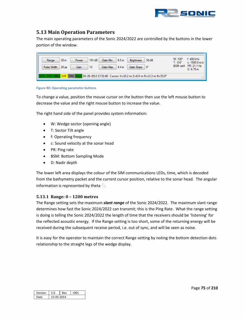
5.13 Main Operation Parameters The main operating parameters of the Sonic 2024/2022 are controlled by the buttons in the lower portion of the window.

Figure 80: Operating parameter buttons

To change a value, position the mouse cursor on the button then use the left mouse button to decrease the value and the right mouse button to increase the value.

The right hand side of the panel provides system information:

• W: Wedge sector (opening angle) • T: Sector Tilt angle • f: Operating frequency • c: Sound velocity at the sonar head • PR: Ping rate • BSM: Bottom Sampling Mode • D: Nadir depth

The lower left area displays the colour of the SIM communications LEDs, time, which is decoded from the bathymetry packet and the current cursor position, relative to the sonar head. The angular information is represented by theta Θ.

5.13.1 Range: 0 – 1200 metres The Range setting sets the maximum slant range of the Sonic 2024/2022. The maximum slant range determines how fast the Sonic 2024/2022 can transmit; this is the Ping Rate. What the range setting is doing is telling the Sonic 2024/2022 the length of time that the receivers should be ‘listening’ for the reflected acoustic energy. If the Range setting is too short, some of the returning energy will be received during the subsequent receive period, i.e. out of sync, and will be seen as noise.

It is easy for the operator to maintain the correct Range setting by noting the bottom detection dots relationship to the straight legs of the wedge display.


Figure 81: Range setting represented in the wedge display

Figure 82: Graphical concept of the Wedge Display

Straight legs of the wedge represent the Range setting; bottom detection dots should be within this area

Straight legs of the wedge represent the Range setting; bottom detection dots should be within this area


5.13.2 RangeTrac™ – Sonic Control automatically sets correct range RangeTrac™ removes the need to manually set the correct range; Sonic Control will determine the correct range and maintain the range setting, no matter how rapidly the depth may change. RangeTrac is enabled by selecting the box, next to RangeTrac, in Sonic Control.

Figure 83: RangeTrac enabled

The Range button will change to reflect that Sonic Control is operating in RangeTrac mode.

Sonic Control will continue to operate in RangeTrac mode until the user manually changes range or RangeTrac is deselected.

When using RangeTrac, the user manually sets the range first and then turns on RangeTrac; from that point on, there is no need for the user to adjust the Range setting. RangeTrac will automatically set the correct Range for the water depth. RangeTrac will also optimise the ping rate for the determined range.

There are no limits to RangeTrac as far as steepness of slope or amount of variability. RangeTrac can be used simultaneously with GateTrac, in both the Depth and the Depth + Slope modes.

5.13.3 Power: 191 – 221 dB The Power setting sets the source level of the transmit pulse; this is represented in Figure 60, below. The Sonic 2024/2022 should be operated with sufficient power to enable good acoustic returns from the sea floor. The value will change based on water depth, bottom composition, and operating frequency. In general, higher power is better for getting decent bottom returns rather than using receiver gain to obtain the returns. If the Power setting is too low, more receiver gain will need to be used to capture the bottom returns; this can mean more extraneous noise will also be received. The increase in noise will require more processing time; it is better to slightly increase the Power to increase the strength of the bottom returns and, thus, allow for a lower receiver gain setting. If too much power is used, the receivers can be over-driven (saturated); this will result in noisy data and/or erroneous nadir depth readings. A good balance of source level (Power) and receiver gain is the desired end. Shift – left click will turn transmitter power off (Power 0).

5.13.4 Pulse Length: 15µsec – 1000µsec Pulse length determines the transmit pulse duration time. The Sonic 2024 pulse length range is from 15µsec to 1000µsec. The pulse length does not affect the pulse amplitude, which is determined by the Power setting. The general guide line is to maintain as short a pulse length as


possible to optimise the resolution, but not so short as to weaken the transmit pulse. Generally, as the water gets deeper the pulse length will have to be increased to get more ‘total’ power in the water. The default pulse length will depend on the chosen operating frequency.

Figure 84: Transmit Pulse

5.13.5 Gain: 1 – 45 Receiver gain is in 2 dB steps from 1 to 45. This adjusts the gain of the sonar head receivers.

5.13.6 Depth Gates: GateTrac™ The depth gate allows the user to eliminate noise or other acoustic interference by the limits set in the Minimum and Maximum Depth. There are manually selected gates, GateTrac: Depth and GateTrac: Depth + Slope.

Gates are enabled by selecting the check box next to Enable Gates.

Figure 85: Enable Gates

Figure 86: Manual and GateTrac selections


5.13.6.1 Gates Manual The depth gates can also be changed using the mouse in the wedge display. Click and drag on either depth gate; the cursor will change to a double arrow , drag the gate to the new depth and release the mouse button. The depth gate position is visible in the lower left hand section of the display. When the mouse button is released the gate will be updated in the Operation Parameters area.

To move both gates, simultaneously, use the right mouse button and both gates will move, keeping the same relationship.

In Manual mode, the gate slope can be adjusted by using the Gate Slope button in the Operation area. The gates can be tilted up to ±90°.

Figure 87: Manually adjust the gate slope

5.13.6.2 GateTrac: Depth GateTrac: Depth will automatically adjust the gates, for water depth, based on the tolerance that is selected by the control next to the gate drop-down menu. The tolerance is ± percentage of nadir depth. Right click will increase the tolerance (up to ±90%); left click reduces the tolerance.

Figure 88: Gate width tolerance toggle

When GateTrac: Depth is enabled, the Gate Min and Gate Max buttons will be disabled, but the Gate Slope button will still be active.

Figure 89: GateTrac enabled; Gate min and max control is disabled

If the soundings are visible, in the display then, when ‘GateTrac: Depth’ is enabled, the gates will automatically jump to the soundings, with the selected tolerance. The user can use the Gate Slope button to change the tilt of the gates, they will still automatically track the bottom, and the gate slope will not change from what the user has selected.


5.13.6.3 GateTrac: Depth + Slope Depth and Slope GateTrac will automatically adjust the gates for the depth and the slope of the bottom. When ‘GateTrac: Depth + Slope’ is enabled, the Gate Min and Max as well as the Gate Slope buttons will be greyed out.

Figure 90: GateTrac: Depth + Slope enabled, manual gate controls are disabled.

Figure 91: GateTrac: Depth + Slope enabled and tracking a steep slope

5.13.6.4 Using Gates If the minimum or maximum depth gate eliminates good data, the data are lost as it will not be included in the Sonic 2024/2022 output. In the data collection software there will also be a form of depth gates. If the data are eliminated there, it is more than likely that the data is flagged and not really deleted, so it can be recovered.

The main reason to use the Sonic 2024/2022 depth gates is to eliminate interference of the bottom detection process. Depending on bottom composition, multiple returns can occur. There will be a secondary and possibly a tertiary return that arises from the initial bottom returns being reflected by the water surface and then back up again to the receiver. These second and third returns can be strong enough to influence the bottom detection process. Using the Sonic 2024/2022 depth gate will enable the Sonic 2024/2022 to search only a small area of the entire beam for the bottom Page 80 of 210 Version 5.0 Rev r001 Date 15-05-2014 Part No. 96000001

detection, therefore, only the area around where the energy from the actual bottom returns are will be searched to derive a bottom detection. Although the user enters a depth for the gate setting, to the Sonic 2024/2022 this is a time to start searching and a time to stop searching.

Figure 92: Graphical representation of depth gate

The above representation illustrates how the depth gate narrows down the bottom detection search area (in time) to only the area where the true bottom is expected. If the Maximum Depth gate was not in this location, the second return could be strong enough so as to influence the bottom detection process.

Again, it must be borne in mind that if the depth gate is set such that true bottom detections are ‘gated out’; those data are lost entirely and cannot be recovered.

5.14 Ruler The ruler or measuring tool can be used to obtain range and bearing information, within the GUI, by using the mouse cursor. Use Ctrl + Left Mouse Button (LMB), the cursor will change to a cross and can be dragged to the target (once the range and bearing is initiated, the Ctrl button can be released. The Range and Bearing information is along the bottom of the Sonic Control window. To remove, the Ruler use Ctrl + Double Click LMB.

Figure 93: Ruler Function


5.15 Save Settings When Sonic Control is launched, it will always load the default settings configuration file located in the Sonic Control installation directory (CurrentSettings.ini). The default configuration file will save any local configuration changes during operation of the system. When a user defined configuration is saved, like dualhead.ini, Sonic Control will still use the default configuration file to store local changes while operating the sonar. This is equivalent to copying the default configuration file to a configuration file with another name. When a user defined configuration is loaded, Sonic Control will use the default configuration file to store local changes while operating the sonar. This is equivalent to copying the loaded configuration file to the default configuration file.

5.16 Operating Sonic Control on a second computer There may be circumstances where it is preferred to run Sonic Control on a different computer than the computer where the data collection software is running. The user can change IP addresses as well as UDP ports. By doing Discover (in Settings | Network Settings), the system looks for all attached R2Sonic equipment, which will be identified by model and serial number. Once the serial number is discovered, it is used to assign an IP and UDP port to the sonar head and the SIM, after this is done, the IP and UDP ports can be changed.

5.16.1 Two computer setup 1) Set the data collection computer’s networking to IP address 10.0.1.102 as usual 2) Setup Sonic Control, on the data collection computer, as normal: do Discover and apply the

settings to establish communication with the system 3) Set the second computer’s networking to IP address 10.0.1.105 (using this as an example) 4) Load Sonic Control on the second computer, but do not connect the second computer to the

SIM until directed to below 5) Open Sonic Control on the second computer 6) Go to Settings | Network settings and change only the GUI IP address to 10.0.1.105 (see

illustration below) 7) Connect a LAN cable from the second computer to one of the free RJ45 ports on the SIM

(there will now be 2 Ethernet cables connected to the SIM) 8) On the data collection computer’s Sonic Control, go to Settings | Network Settings and

change only the GUI IP to the IP of the second computer: 10.0.1.105 (see illustration below) 9) Do not change any other IP or Port, only the IP for the GUI is to be changed 10) Select Apply: the GUI, on the data collection computer, will no longer update nor will it be

able to control the multibeam 11) On the second computer, open Sonic Control 12) Under Network settings, use Discover to obtain the serial numbers of the SIM and sonar

head and Apply; this computer now controls the Sonic system. Page 82 of 210 Version 5.0 Rev r001 Date 15-05-2014 Part No. 96000001

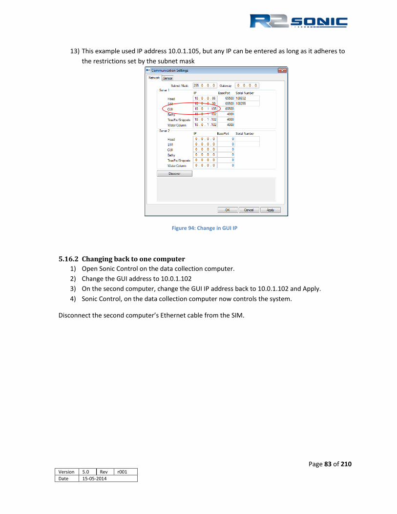
13) This example used IP address 10.0.1.105, but any IP can be entered as long as it adheres to the restrictions set by the subnet mask

Figure 94: Change in GUI IP

5.16.2 Changing back to one computer 1) Open Sonic Control on the data collection computer. 2) Change the GUI address to 10.0.1.102 3) On the second computer, change the GUI IP address back to 10.0.1.102 and Apply. 4) Sonic Control, on the data collection computer now controls the system.

Disconnect the second computer’s Ethernet cable from the SIM.



6 SONIC 2024/2022 THEORY OF OPERATION The Sonic 2024/2022 transmits a shaped continuous wave pulse at the user- selected frequency. The transmit pulse is narrow in the alongtrack direction, but very wide in the across-track direction. The reflected acoustic energy is received via the Sonic 2024/2022 receivers; within the Receive Module the beams are formed and the bottom detection process takes place. The resultant bottom detections (range and bearing) are then sent via Ethernet, through the deck lead, to the SIM. The SIM then sends the data out to the Sonic Control software and the data collection software.

6.1 Sonic 2024/2022 Sonar Head Block Diagram

Receive Module Re

ceiv

ers

Wet Controller

Beam Former

Bottom Detection

To SIM Gigabit Ethernet

Transmitter Board

Proj

ecto

r

Transmitter Power Supply

Low Voltage Power Supply

Med. Voltage Power Supply

48 DCV from SIM

Figure 95: SONIC 2024 Sonar Head Block Diagram


6.2 Sonic 2024/2022 Transmit (Normal Operation Mode) The projector is comprised of a precisely arranged set of composite ceramics. The projector, itself, can transmit over a wide frequency range, which makes it unique amongst multibeam echosounders. A pulse, at the chosen operating frequency, excites the ceramics which converts the electrical energy to acoustic energy. The pulse originates from the Wet Controller board in the Receive Module, which is then passed onto the Transmitters and out to the Projector. The amplitude of the pulse is set by the transmit Power setting in Sonic Control 2000; the Pulse Length setting in Sonic Control 2000 determines how long the pulse excites the ceramics.

The projector’s transmit pattern ensonifies the seafloor in a very wide across-track, but narrow along-track pattern as the vessel moves along the survey line. The across-track angle is 160°; the along-track angle depends on frequency. The 400 kHz along-track pattern is 1°. The along-track lengthens out to 2° at 200 kHz. This is the Normal Operating Mode and not extended Vertical Mapping Mode.

Figure 96: Transmit pattern

Depending on the water conditions, sea floor composition and other factors, a portion of the acoustic energy that strikes the seafloor will be reflected back towards the surface. The return acoustic energy will strike the Sonic 2024/2022 receiver’s ceramics.


6.3 Sonic 2024/2022 Receive (Normal Operation Mode) The Projector is comprised of composite ceramics that convert electrical energy to acoustic energy. The composite ceramics, in the Receive Module, convert the reflected acoustic energy back to electrical energy. The small electrical voltage, generated by the ceramics, is amplified and then passed onto the receivers. The output of the receivers goes directly to the Wet Controller board in the Receive Module.

In general, the receive pattern is 130° (normal bathymetry survey) in the across-track. The along-track pattern depends on the frequency; from 23° at 400 kHz to 40° at 200 kHz.

Figure 97: Receive pattern with Transmit pattern

The Wet Controller board contains the FPGA that performs the beam forming and bottom detection operation; time tags the data; and formats the sonar data for output back up to the SIM. The bathymetry data is output as a Range and Bearing (from the sonar head’s acoustic centre) for each beam. Other outputs include: side scan, beamformed imagery, and Snippets.

The output of the Wet Controller board is sent through the deck lead, to the SIM’s Gigabit switch and onto the data collection computer though one of the SIM’s external RJ45 connections.



6.4 Sonic 2024/2022 Sonar Interface Module (SIM) Block Diagram

Figure 98: Sonar Interface Module Block Diagram

6.4.1 Sonar Interface Module (SIM) Block Diagram

6.4.1.1 SIM Power Requirement The SIM operates within a voltage range of 90 to 260 VAC. The mains voltage is converted in the various DC voltages required for the operation of the Sonic 2024/2022. Primarily, 48 VDC is sent to the Receive Module to power the sonar head.

6.4.1.2 SIM Controller The SIM Controller card primarily does time stamping of sensor data and deals with RS-232 and BNC data.

6.4.1.3 SIM – Sonic Control 2000 interfacing Sonic Control 2000 communicates with the SIM over the Gigabit Ethernet DATA RJ-45. Commands, from Sonic Control 2000 are transmitted to the SIM and then to the Sonic 2024/2022. The Sonic 2024/2022 data passes through SIM to the data collection software.

6.4.1.4 SIM – RS-232 / Ethernet Interfacing The SIM receives the GPS PPS and time message (NMEA ZDA), the sound velocity from the probe near the sonar head and the motion sensor data (for roll stabilisation only). These data are routed through the SIM Controller to the Ethernet switch for transmission to the sonar head.

48VDC

48VD

C

I/O

Boa

rd

RS-232

TTL - BNC

RS-232

Gigabit Ethernet

SIM Controller

Gigabit Ethernet Switch

Power Supply

Sonar Connector

To/From Sonar Head

90 – 260 VAC



Appendix I R2Sonic I2NS™

7 Appendix I: R2Sonic I2NS Components and Operation The R2Sonic I2NS (Inertial Navigation System) option integrates the Applanix Position and Orientation System (POS/MV)’s POS Computing System (PCS) and Sonar topside units saving both power and space while simplifying vessel mobilization. The setup of the R2Sonic INS is identical to the setup of the Applanix POS/MV system; POSView (Version 7.60 or more recent) is necessary for inputting offsets and configuring outputs. All of the data, both sonar and POS/MV are sent over the one Ethernet cable to the data collection computer; eliminating the need for two network cards. The information contained here does not detail the POSView software to set up the Applanix POS/MV; that information is found in the Applanix POS/MV manual. The information provided here covers the necessary setup of the R2Sonic I2NS components as relates to the R2Sonic SIM and Sonic Control. Where necessary, certain steps in the POSView software are detailed.

The R2Sonic INS will work on all R2Sonic systems with SIM firmware: Simb$26-OCT-2013-15-58-27.bin and head firmware: Head$16-Nov-2013-04-35-57.bin or more recent.

7.1 Components The R2Sonic I2NS is comprised of the enhanced Sonar Interface Module (SIM), which contains the Applanix boards and connections for the antennas and Inertial Measurement Unit (IMU). Two antennas (and cables) and one IMU (and cable) complete the physical INS components.

Figure 99: R2Sonic I2NS Main Components (not including antennas and cables)

Figure 100: GNSS Antennas


7.2 Connection diagram When using the INS, there is no need to provide inputs for the motion or the time stamp, as those are provided internally, through the SIM’s Gigabit switch. The only serial connection is the sound velocity probe that is on the sonar head. A PPS loop cable is required to go from the PPS out to the PPS in.

Figure 101: INS connections

Figure 102: INS SIM block diagram


7.3 Installation

7.3.1 The IMU and GPS antennas The IMU (Inertial Measurement Unit) housing should be secured by 4 M8 (5/16” in Imperial units) screws. The IMU housing is depth rated to 15m. The IMU can be mounted close to or on the Multibeam transducer itself. It is not necessary to mount the IMU at the vessel’s CoG (centre of gravity), but if it is not mounted on the CoG, it is vitally important that very accurate IMU to CoG offsets are input into POSView. The GNSS antennas should be mounted rigidly with respect to each other as well as the IMU, with a separation of at least 1m between the GPS antennas. The antennas should be mounted so that they have a clear view of the sky. The standard cables provided with the INS option are: 1x15m IMU cable 1xBNC jumper cable 2x8m GPS antenna cables

7.3.2 INS BNC – TNC Connections

Figure 103: INS BNC & TNC Connections

Figure 104: PPS Out - PPS In

There is one BNC connection for the PPS out. The TNC connection next to it is for the Primary Antenna. The Secondary antenna connects to the TNC connection on the end.

The PPS Out is connected to the SIM PPS In, with a short length of cable


7.3.3 I2NS DB9 Connections The I2NS has two serial communication ports. These are standard DB9M serial connections that are setup in the POSView software. Both ports are bi-directional and can be configured to receive RTCM corrections or to output standard NMEA or binary serial data. For full information on the serial ports, please refer to the POSView documentation.

Figure 105: Com 1 and Com 2 on SIMINS for POS MV serial data

In POSView, in the Input/Output Ports Set-up, only COM 1 and COM 2 are to be configured.

Figure 106: POSView Serial port setup


7.4 Setup in Sonic Control

7.4.1 Network Setup In the event that the Applanix IP address is lost and no connection can be made through POSView it can be reset through the R2Sonic GUI. To change the IP address of the POS/MV, reboot the SIM box, open the R2Sonic GUI and go to Settings>Network Settings and under “INS IP” enter the desired IP. The POS/MV takes approximately 2 minutes to power on, once the POS is fully booted, the IP can be set in the R2Sonic GUI. Once the POS is fully booted the user has 5 minutes to change the IP address of the POS/MV. Attempting to change the IP address, outside of the 5 minute window, will result in a warning that the SIM box must be rebooted before changing the INS IP.

Figure 107: Network Settings SIMINS

Figure 108: Cannot Change IP, waiting on msg 32

Figure 109: Set IP time expired, cannot change IP

0 minutes: turn on 0 to 1min: Button label is "Set IP wait" and button text is greyed out. The INS IP cannot be updated during this period. The GUI is waiting for the INS to send out message 32. After ≈ 1 - 2 mins: the GUI will allow changes to the INS IP address. The actual time depends on when the GUI starts receiving message 32 from the INS. From ≈1min (2min) to 7min: INS IP address can be changed. Button text turns from greyed out to black text and says "Set IP". After 7 min: INS won't accept change in IP address. Button text color is greyed out and label says "Set IP expired".


7.4.2 Applanix Group 119 specific to R2Sonic SIMINS Src: 10.0.0.44:65533 Dst: 10.255.255.255:5606 Applanix POS, Customer data Group 119 (MV customer defined group) Group start: $GRP Group ID: 119 (MV customer defined group) Byte count: 132 Time/Distance Fields: Time 1: 358370.467027857 (UTC seconds of the week) (Thu 03:32:50.467028 UTC) Time 2: 1091.53761465444 (POS seconds since power-on) (0.303205 hours) Distance tag: 0 (POS distance) Time types: 0x02 Distance type: 0x01 User ID: 1 Reserved: 00 PacketName: R2A0 PacketSize: 100 Reserved0: 0000 PpsTime: 358386 (GPS seconds of the week) (Thu 03:32:50.000000 UTC) (1395286370 Unix) VesselLatitude: 30.2391284856087 (degrees) VesselLongitude: -97.838843091206 (degrees) VesselAltitude: 198.64372053742 (meters) North position RMS error: 0.922135 (meters) East position RMS error: 0.698561 (meters) Down position RMS error: 1.10037 (meters) VesselPitch: 0.00230865 (radians) (0.132276 degrees) VesselRoll: 0.000915637 (radians) (0.052462 degrees) VesselHeave: 0.0256301 (meters) VesselHeading: 0.115629 (radians) (6.625050 degrees) RmsErrorPitch: 0.0292523 (degrees) RmsErrorRoll: 0.0292523 (degrees) VesselSpeed: 0.063469 (meters/second) RmsErrorHeading: 10.2586 (degrees) GpsWeekNumber: 1784 (GPS weeks) UTCTimeOffset: 16 (GPS-UTC seconds) StatusB: 0x0189200d StatusC: 0x00001000 StatusExtended: 0x00000100 Satellites: 9 Reserved1: 00 Reserved2: 0000 Checksum: 23896 (Good) Group end: $#


7.4.3 Sensor Setup All of the required information (time message and motion data) from the INS stack, except for the PPS, is transferred internally. However, in the Sensor setup the Interface type and Ethernet configuration has to be set up to receive the internal information. The GPS and Motion interface type is set to Ethernet. The IP that the POS/MV stack sends data out is 10.0.0.44 and uses UDP port 5606, which is unique for R2Sonic requirements. The POS/MV Ethernet data, going to the data collection computer, is on the same IP (10.0.1.102), as the sonar data and uses the standard POS/MV UDP 5602. If the data collection software requires the IP address of the ‘talker’, the POS/MV stack outputs on IP 10.0.0.44.

Figure 110: Sensor setup for SIMINS

7.4.4 INS Monitor (Alt+I) INS data can be monitor through the INS monitor. The INS monitor option is under Status.

Figure 111: INS Monitor

The INS Monitor allows the user to constantly monitor the values from the INS.

In POSView, the user sets up the User Accuracy (under Settings | Installation), these values are used, by the INS Monitor, if a value exceeds the entered user accuracy, the reading will be in red, as seen in the figure.



7.5 Measuring IMU Offsets

Figure 112: IMU Reference indicators

Identify the COG of the vessel that point becomes the reference point of the INS offsets. The POS/MV uses a right-hand Cartesian co-ordinate system therefore the lever arm offsets should be measured as

+X = To Bow +Y = To Starboard +Z = Down

When using DGPS offsets should be measured to 5cm accuracy. When using RTK offsets should be measured to 5mm accuracy. Measure the offset from the reference point to the primary GPS antenna and record it in POSView in the “ref. to Primary GPS Lever Arm” fields. There is no need to measure the offset of the second antenna; the Applanix GAMS calibration will determine this X offset. Measurement of the IMU COG is critical. The IMU has two reference points. On top of the IMU is the horizontal reference for the X and Y measurement. The vertical Z reference is measured to the reference point on the rear part of the IMU. After measuring the reference to IMU offsets, input the values in the “Ref. to IMU Target” fields in POSView Be sure to check the box by “Enable Bare IMU”, as seen below. NOTE: Some older versions of POSView will not have this option. If not, please install the version preloaded on the R2Sonic CD that shipped with the Sonar.

Horizontal Reference

Vertical Reference


Figure 113: POSView Lever Arm setup

Figure 114: View of installation with the entered offsets

If the Reference point chosen is NOT the COG of the vessel input the offsets from the ref to the COG in the “Ref. to Centre of Rotation” fields. This step is extremely important for accurate heave information to be reported.

Use the View, when entering offsets, so that the correct sign is confirmed. This figure represents the physical installation, using the offsets that are seen in the above figure.


7.6 I2NS Physical Specifications

Table 9: I2NS Dimensions and Mass

Component Dimensions (L x W x H) / Mass I2NS Sonar Interface Module (INS-SIM) 280mm x 170mm x 126.4mm (top of cooling fins) / 4.17kg Inertial Measurements Unit (IMU) 161mm x 140mm x 110m / 2.2kg GNSS Antenna Ø178mm x 73mm / 0.45kg

Table 10: Electrical Specifications

Item Specification INS (SIM, IMU & Antennas) 38.4w INS + Sonic 2024 88.4w INS + Sonic 2022 73.4w



7.7 I2NS Drawings

7.7.1 I2NS IMU

Figure 115: IMU Drawing


7.7.2 I2NS Sonar Interface Module (SIM)

Figure 116: I2NS SIM Drawing


APPENDIX II: Multibeam Survey Suite Components

8 APPENDIX II: Multibeam Survey Suite Components

8.1 Auxiliary Sensors and Components A multibeam survey system is comprised of more components than just the Sonic 2024/2022 Multibeam Echosounder. These components are the auxiliary sensors, which are required to provide the necessary information for a multibeam survey. This does not mean that these sensors are a minor part of the survey system; each auxiliary sensor is required for any multibeam survey operation. The required sensor data:

• Position: Differential Global Positioning System Receiver • Heading: Gyrocompass • Attitude: Motion Sensor • Refraction correction: Sound Velocity Probe

Each of the individual sensors requires their own setup and operation procedures. The details, discussed here, concerning the installation and calibration of the auxiliary sensors, is supplemental to any and all manufacturer’s documentation.

8.2 Differential Global Positioning System The Global Positioning System (GPS) is well known to all surveyors. There was a period of time when the GPS position was intentionally made less accurate; this was Selective Availability (SA). When SA was enacted, the GPS position became too inaccurate for survey use. It was during this period that the concept of differential corrections was established. Differential corrections were derived from users monitoring the GPS position at a known survey point and computing the corrections required to adjust the various pseudo ranges to make the GPS position agree with the known survey position. If a vessel was operating within the local area and observing the same satellite constellation, the derived pseudo range corrections could be applied on board to make for a more accurate and consistent position. The corrections are normally transmitted over a radio link and applied within the GPS receiver.

8.2.1 Installation The first and foremost consideration when installing the DGPS system is the location of the respective antennae. Both the GPS antenna and the differential antenna (if they are two separate antennae) need to be mounted on the vessel in such a way so as to have a totally unobstructed view of the sky.


When installing the GPS antenna, the surveyor should be aware of the position of the stacks and masts; in particular are davits or cranes that may be currently in a stored position, but will be in use during survey operations. If mounting the antenna on a vessel that has helicopter landing facilities, coordinate the placement of the antenna with the personnel in charge of helicopter operations.

When the location for the antennae has been determined the next step is determining how the coaxial cable, connecting the antenna and the receiver, is to be run. The cables should be run in such a manner so as to be protected from possible damage. Cables should not be run through hatches or windows, if it can be avoided; if such runs are necessary, then a block or other such obstruction should be placed so that the hatch or window will not close on the cable. If the cables are to be suspended between two points, a rope or other line should be strung to carry the weight of the cables. Cables should never be kinked; all cables have a minimum bending radius, if it is known adhere to it, if it is not known, use common sense. Do not run cables in a manner that they will become safety hazards on the vessel, causing personnel to trip or be caught on them. Avoid running cables along voltage carrying lines.

It is important to mark the cables at both ends to denote what they are and to where they go.

The connection to the antenna may be required to be completely water proofed (depending on the manufacturer’s recommendations) using electrical tape, with a secondary covering of self-amalgamated tape. Ensure that there are no air gaps in the tape; they will become a channel for water. If a cable is to be run upwards from the antenna, form a drip loop by leaving slack in the cable that will hang below the antenna connector. This will allow any water that flows down the cable to collect and drip from the slack loop instead of running into the connector.

The cables, connectors and antennae should be inspected regularly for signs of damage, corrosion or abuse. Any abrasions on the cable should be securely taped; if possible, a waterproof coating should also be applied.

8.2.2 GPS Calibration Prior to commencing survey operations, the accuracy of the Differential GPS position and transformation to local datum should be determined. There are two main methods to determine the accuracy of the DGPS position and data transformation. For both methods, a local land survey benchmark is required.

8.2.2.1 Position Accuracy Determination Method 1 The GPS antenna is physically placed over the survey benchmark. The surveyor will ensure that the antenna has a clear view. This is particularly important if the benchmark being used is in a dock area. The surveyor will also ensure that, if a separate antenna is used to receive differential corrections, that it is not blocked.

The GPS position data should be logged, in the data collection software, for not less than 15 minutes. The collected data can then be averaged, standard deviations determined, and compared to the published position of the survey benchmark. Page 106 of 210 Version 5.0 Rev r001 Date 15-05-2014 Part No. 96000001

The two main causes of error, in this area, are:

• Wrong geodetic transformations being applied to the WGS-84 position derived from GPS. • Erroneous coordinates for the Differential reference station.

8.2.2.2 Position Accuracy Determination Method 2 This method is most easily accomplished during the gyrocompass calibration. The antenna remains mounted on the vessel. The surveyor will set up on the known survey benchmarks; using standard land survey techniques, the exact absolute position of the antenna can be determined. During the period that the surveyor is ‘shooting in’ the GPS antenna, the GPS position will be logged on board, the averaging and statistical analysis will be as above.

The surveyor will need to take numerous shots to also obtain an average, due to the possible movement of the vessel while alongside.

8.3 Gyrocompass Utmost care is required for the installation of the gyrocompass. The gyrocompass is a sensor that cannot be situated randomly. The purpose of the gyrocompass is to measure the vessel’s heading. In order to do this, the gyrocompass should be placed on the centre line running from the bow stem to the midpoint of the stern. If it is not possible to place the gyrocompass on the centreline of the vessel, it can be mounted on a parallel to the centre line.

All survey grade gyrocompasses will be plainly marked for alignment on the centre line. This marking may be an etched line fore and aft on the mounting plate, or possibly metal pins on the front and the back of the housing that point down. If no marking exists, then measuring the fore and aft faces and finding the centre may be sufficient.

No matter how well the gyrocompass is placed, there exists a possible error between the true vessel’s heading and the gyrocompass derived heading. Any new installation of a gyrocompass should include a gyrocompass calibration. There are various methods to perform a gyrocompass calibration; the best method employed will be determined by the location of the vessel, the time allotted for the calibration and the resources at hand.

8.3.1 Gyrocompass Calibration Methods After the installation of gyrocompass (henceforth termed gyro) on a vessel, that gyro should be calibrated to ensure that the heading it determines is the true heading of the vessel.

If the error is large, the gyro can be physically rotated to align itself with the true vessel heading. Small errors can be corrected, either by internal adjustment to the gyro, or in the software that receives the gyro reading.


8.3.1.1 Standard Land Survey Technique One of the most accurate methods to determine the gyro error involves the use of standard recognised land survey techniques. The time and equipment involved requires that a substantial period be allotted for such a calibration.

• If possible, the vessel will be berthed alongside a quay or dock that has a survey benchmark located in close proximity.

• If a survey benchmark is not located close to the berth, then the surveyor will have to run a transit from the nearest, suitable, local survey bench mark to establish a point on the quay that has a well-defined position. From this point another point should be established along the quay to form a baseline.

• When the vessel comes alongside, all lines should be made as taut as possible. The gyro should be allowed 2 hours to settle down after the vessel has come alongside.

• The stern of the vessel should be measured, with a metal tape, to determine the centre point of the stern. A survey reflector will be placed at this position. Another survey reflector will be placed exactly at the bow. It will be verified that the reflectors are accurately placed on the centre line of the vessel by either measurements or survey techniques.

• The surveyor will set up on one benchmark; a round of readings will be taken from the benchmark to the fore and aft reflectors. Simultaneous to this, the survey personnel will record the gyro heading as it is read by the survey computer. Any variation between the digital output and the physical gyro reading should be remedied prior to the commencement of readings. It is recommended that the personnel on the vessel and the surveyors on the quay be in constant communication to assist in coordinating the measurements.

• One round of readings will be considered to be not less than 30 sets, a set being one reading each from the bow and stern reflectors.

• Upon completion of the round from benchmark one, the surveyor will move to benchmark two and repeat the process.

• Upon the completion of all rounds, from the two benchmarks, the vessel will turn about. With the vessel, now heading on the reciprocal heading, the gyro will be allowed at least 1 hour to settle down.

• When the gyro has been given sufficient time to settle down, a further series of range and bearing measurements will be made in exactly the same manner as before.

When all readings are completed, the surveyor will calculate the azimuth between the two survey reflectors for each set of readings. The azimuth readings will be compared with the headings taken on board the vessel from the gyro itself. If there has been little or no movement of the vessel, an average can be taken of the azimuths and for the gyro readings and compared. By calculating the standard deviation of the readings, the surveyor can determine the degree of movement during the recording process. If the deviation is greater than the stated accuracy of the gyro, the comparison readings should be based on simultaneous time.


If physical adjustments are required, they should be made and the calibration process repeated. If the adjustment is determined to be minor and can be accounted for in the survey software, the correction value should be entered and then verified using the calibration process. This check of the calibration value can be an abbreviated version of the calibration process detailed above.

Figure 117: Gyrocompass Calibration method 1

• Quayside Benchmarks have known geodetic positions. • Measure Range and Bearing to reflectors on vessel centre line. • Using Range and Bearing to reflectors, determine geodetic position for

reflectors. • Calculate bearing from stern reflector to bow reflector will give the true

heading of the vessel. • True heading of vessel is then compared to gyrocompass reading taken at

the same time as the Range and Bearing measurements. • Benchmarks do not have to be on the quay, but should be in a position to

give accurate Range and Bearing to the reflectors.


8.3.1.2 Tape and Offset Method of Gyro Calibration This method relies on measuring the offset distance from a baseline on the quay, with a known azimuth, to a baseline that is established on the vessel. There are greater areas for error when using this method, particularly in establishing a baseline with known azimuth.

A baseline is established on the quay as close as possible to the vessel's side. It is very important that the azimuth of this baseline be as accurately determined as possible. The baseline should be of a length that will exceed the baseline that is established on the vessel.

A baseline is established on the vessel that is parallel to the centre line of the vessel. It should not be assumed that the side of the vessel is parallel to the centre line. This baseline should be on the deck that faces the dock. The baseline on the vessel should be as long as possible, the longer the better.

With the vessel secured alongside the quay, the vessel baseline will be compared to the quayside baseline. Two points will be established on the quayside baseline that corresponds exactly to the fore and aft positions on the vessel baseline. That is: the points that are established on the quayside baseline should be normal to the points on the vessel baseline.

Figure 118: Gyro Calibration Method 2


The example, below, will illustrate the math involved.

Figure 119: Gyro Calibration Method 2 example

A to A' 1.0 metres B to B' 1.5 metres

Side a 5.0 metres Side b 1.5 – 1.0 = 0.5 metres

Angle b' Arctan 0.5/5.0 = 5.7°

Ship Azimuth = 270° + 5.7° = 275.7°

Table 11: Gyro Calibration Method 2 computation

Figure 120: Idealised concept of Gyro Calibration Method 2

In this example, the vessel heading for this set of readings is 275.7°; this would be compared to the gyro reading recorded at the same time the offsets were measured. In the above example, if the bow was further out from the quay than the stern, the angle b' would be subtracted from the azimuth of the quay, i.e. 270° - 5.7° = 264.3°.


8.4 The Motion Sensor The motion sensor is used to determine the attitude of the vessel in terms of pitch, roll and heave. Pitch is the movement of the bow going up and down. Roll is the movement of the port and starboard side going up and down. Heave is the vessel going up and down.

The sonar head is physically attached to the vessel; as the vessel moves, so does the sonar head. The motion sensor reports the movements of the vessel to the data collection software; the data collection software, using the offsets to the motion sensor and to the sonar head, computes the movement at the sonar head to correct the multibeam data for pitch, roll and heave.

One important aspect of the motion sensor is the sign convention used by the motion sensor as compared to the sign convention used in the collecting software. The surveyor must be aware of the convention that is used and what adjustments are necessary, if any, to ensure that the convention is consistent with the data collection computer.

There exist two major areas of thought as to where the motion sensor should be situated. One group believes that the motion sensor should go as close to the multibeam as possible, even if the multibeam is mounted on an over-the-side pole. The second group believes the motion sensor should be placed as close to the centre of rotation for the vessel as possible.

Placing the motion sensor on the hydrophone pole would seem to solve for all movement of the pole itself, but in fact the motion sensor, mounted in this fashion, can provide false attitude measurements. This is particularly true when there is significant roll; the motion sensor on the pole can interpret a portion of this roll as heave, which is not true. By placing the motion sensor as close to the centre of rotation (also called the centre of gravity) as possible, only the real heave of the vessel will be measured. All software will solve for the motion of the sonar head, based on the offsets that have been entered into the setup files for the vessel configuration; this is called a lever arm adjustment. The other consideration is that the motion data is usually applied to the GPS antenna. The GPS antenna is usually mounted high on the vessel, so any pitch or roll will induce a large amount of movement in the GPS antenna thus providing a false position due to the antenna movement. If the motion sensor is mounted on the hydrophone pole, it is reporting an exaggerated motion because it is far from the centre of motion of the vessel; this exaggerated motion then would be applied to the GPS antenna position and the vessel position computation would be in error.

The other consideration is that the alignment of the motion sensor must be on or parallel to the centre line of the vessel; it is essential to prevent ‘bleed-over’ of pitch and roll. If the motion sensor is not aligned with the centre line, when the vessel rolls some of the roll will be seen as pitch as the motion sensor’s accelerometers and gyros are not aligned with the axes of the vessel it is mounted on. It is more difficult to obtain this precise alignment if the motion sensor is placed on the pole.

Mount the motion sensor as close to the centre of rotation (or centre of gravity as possible) and perfectly aligned to the centre line of the vessel.


The motion sensor should be mounted on as level a platform as possible. After mounting the motion sensor, the actual 'mounting angles' should be measured. Some motion sensors contain internal programs that can measure the mounting angles. Some data collection software packages also include the capability to measure mounting angles. The mounting angles are the measured degrees of the actual physical mounting of the motion sensor. This is to compensate for sloping or warped decks. Many decks have some slope to them and this should be accounted for to ensure that the pitch and roll values that the motion sensor derives is for vessel movement and not for its physical mounting on the deck. The mounting angles should be measured prior to any multibeam calibration and not changed after the calibration.

Prior to measuring the mounting angles, the vessel should be put in good trim by the engineer. On a small vessel it is important that the angles be measured without undue influence from people standing around. A false measurement can be induced by two people sitting on the gunwale having a conversation while the measuring process is being completed. It is usually a good idea to have all personnel leave a small vessel during the measuring process.

If the motion sensor mounting angles have been entered in the motion sensor or the data collection software, they can only be changed prior to the multibeam calibration (patch test); they are not to be changed after the patch test.

It is important to keep the motion sensor in mind when surveying. A motion sensor takes time to 'settle down' after a turn or a speed change and most of the settling down will depend on the heave bandwidth that is entered into the motion sensor. Some motion sensors can take in position, speed and heading data to assist them in the settling process. Depending on the degree of the turn or the amount of the speed change a practical period of 2 minutes should be allowed for the motion sensor to settle. It is prudent to plan the survey to allow for a long enough 'run-in' to the start of data collection to allow the motion sensor time to settle and the heave normalise. If this is not done, many times motion artefacts or erroneous depths will be seen at the beginning of line and the processed data will not be correct.

Monitor the motion sensor (all data collection software provides a time series window to monitor individual data) to ensure that it is operating properly.

8.5 Sound Velocity Probes There are two basic types of sound velocity probes. One type measures the parameters of sound velocity in water; those being Conductivity (Salinity), Temperature, and Depth (Pressure), these are normally referred to as CTD probes. The other type of probe contains a small transducer and has a reflecting plate, at a known distance from the transducer that reflects the sound, the time is measured for this transmission and the sound velocity determined by that measurement; these are called Time of Flight probes. There is third type, known as the Expendable Bathythermograph (XBT) which is launched and as it passes through the water column sends back temperature readings (through two very thin wires); it is not recovered, it is expendable.


The CTD and Time of Flight probes store the data internally. The data is downloaded to a computer after the probe is recovered.

8.5.1 CTD Probes The CTD probe type of sound velocity probe has instruments to measure the conductivity of the water, water temperature, and a pressure sensor to measure depth. The CTD probe is a good choice if any of this information is also required; to obtain a velocity a formula must be used.

There are various formulae available that are based on the parameters that are recorded by the CTD. The UNESCO algorithm is considered a universal standard and was put forth by C-T. Chen and F.J. Millero in 1977. The Chen-Millero (and Li) equation is complex as is Del Grosso’s (1974) and have been termed Refined. Simple formula, such as Mackenzie’s (1981), also yields good results.

When using a CTD, it is very important that the probe be allowed to sit, fully submerged, in the water for a few minutes prior to deploying it; this is to allow the probe to reach equilibrium with the water temperature It is also important that the tube, through which the water flows pass the sensors, is checked for obstructions or marine growth.

Figure 121: CTD Probe


8.5.2 Time of Flight Probe The Time of Flight probe incorporates a transducer that transmits an acoustic pulse that reflects back from a plate that it is at a very precise distance from the transducer. The two-way travel time is measured, divided by 2, and the sound velocity determined. The Time of Flight probe is usually considered more accurate for multibeam survey work.

The sound velocity probe that is mounted close to the Sonic 2024/2022 sonar head is a time of flight probe.

Figure 122: Time of Flight SV probe

8.5.3 XBT Probes The XBT is a probe which free falls through the water column at a more or less constant speed (the probe is designed to fall at a known rate so that the depth can be inferred) and measures the temperature as it passes through the water column. Inside the probe is the thermograph, which is attached to a spool of very fine wire. Two very small wires transmit the temperature data from the probe back to a computer. The XBT is not recovered. XBT probes can be launched whilst underway

Transducer Pressure sensor

for depth

Reflecting Plate


and are used extensively by Navy and Defence forces for rapid determination of the sound velocity without stopping the vessel.

8.6 The sound velocity cast There are no set rules for when to take a measurement of the water column sound velocity. Common sense is a good guideline. The conditions, detailed below, have a major influence as to when to take a sound velocity cast.

8.6.1 Time of Day Throughout the day the upper level sound velocity characteristic will change mainly due to solar heating or cooling due to cloud cover or precipitation. Another main element of the time of day changes is tides.

When working in tidally influenced areas, the sound velocity can change drastically due to a salt wedge that moves in and out with the tide. The surveyor must be aware of the relationship of the time of the tide to the salt wedge.

8.6.2 Fresh water influx Any river, stream or runoff will drastically change the sound velocity through the introduction of freshwater and also through a temperature difference.

8.6.3 Water Depth The sound velocity cast should always be made in the deepest part of the survey area. The sound velocity profile cannot be extrapolated to deeper depths as there are too many possible variables.

8.6.4 Distance If the survey area is large, then it is quite possible that there will be differences across the range of the survey area even in open water.

8.6.5 Deploying and recovering the Sound Velocity Probe The guide lines for deploying and recovering the sound velocity probe are based on common sense, but are sometimes ignored during the actual operation. The guidelines, below, are for a hand cast in shallow water. The softline, used for the cast, should be marked to provide an indication of the amount of line out.

8.6.5.1 Shallow water sound velocity cast / deployment by hand 1. Plan where the cast is to be made.

a. In a small area, deploy in the deepest part of the survey area. b. Always do a cast prior to starting the survey.

2. Liaise with the captain or office of the watch with the plan position and time of deployment and time required for the cast.

3. Prepare the probe for casting (some probes may need to be programmed prior to each launch).

4. Secure the probe to the downline with a bowline knot or shackle.


5. Secure the bitter end of the downline to the vessel. 6. Request permission, from the bridge or helm, to deploy and await their OK to launch.

a. Bridge or helm to ensure that the vessel is out of traffic. b. Bridge or helm to assess wind and sea conditions and advise as to which side of

vessel the deployment should be made. 7. Put the probe in the water until it is totally covered and let it remain there for a period of

time to acclimate to the sea temperature. This is very important with a CTD type of probe, but of less concern for a time-of-flight probe.

8. Verify the water depth. 9. Lower the probe at a constant rate; only the downcast should be used. 10. Try not to allow the probe to touch the bottom. 11. Recover the probe rapidly. 12. As soon as the probe is on deck, notify the bridge or helm that they are free to manoeuvre,

but remain in the area. 13. Rinse the probe with fresh water and dry thoroughly. 14. Download the cast and verify that it looks good. 15. Load the cast into the data collection software.

8.6.5.2 Deep Water Cast / Deployment by mechanical means A cast in deeper water requires more preparation and planning. A deep water cast can be considered to be any cast that is deployed via an ‘A’ Frame, winch, or other mechanical means. Even a shallow water cast can fall under this definition when mechanical means are used.

One of the main concerns, in a deep water cast, is that the probe will not go straight down due to the current flow or vessel drift due to wind and/or currents. This being the case, weights must be used to ensure the cable (and probe) go as straight down as possible.

Unless the sound velocity probe is designed to have additional weight attached to it, no weights should be attached to the sound velocity probe. The weights, which enable deployment as straight as possible, are attached to the end of the cable. The probe should be attached to the cable approximately 3 – 5 metres above the weights; if the weights hit the bottom this should provide enough scope for the probe to land clear of the weights.


Figure 123: Deploying a sound velocity probe via a winch or A - Frame

The other major consideration, when deploying a probe in deeper water, is that the vessel must be stationary longer and will drift. If there is a large variation in depths, the depth where the probe went in, may not be the same depth when the probe reaches the bottom. It is essential that enough cable be deployed to ensure a full profile to the sea floor.


APPENDIX III: Multibeam Surveying

9 APPENDIX III: Multibeam Surveying

9.1 Introduction Multibeam surveying affords the surveyor with many advantages, but it also requires more thought behind the survey itself.

9.2 Survey Design Multibeam surveying survey planning is very different than single beam survey planning. The main considerations are line spacing and line direction. In single beam surveying, lines are normally spaced based on the scale of the desired chart. The line direction is normally at the discretion of the surveyor. In multibeam surveying, the surveyor has to plan the survey carefully, with thought to overlap between adjacent lines and the direction that those lines are run.

9.2.1 Line Spacing The entire concept of multibeam surveying is based on the swath coverage that defines the multibeam system. The survey lines should be designed so that there is 100% overlap in coverage between adjacent lines. As swath width is a function of water depth, it follows that the spacing between lines may not be constant. Looking at a chart of the survey area, the surveyor should be able to determine the swath width that will be obtained and can design the line spacing accordingly.

A large overlap in swath coverage is required due to various factors. One prime factor is roll. As the vessel rolls the swath coverage will vary in relation to this roll. If the vessel rolls to port (port-side down), the swath coverage on the port side will be lessened, whereas the swath coverage on the starboard side will increase. If there is not sufficient overlap in swath coverage there could be gaps in coverage, between adjacent lines, due to the roll.

If the helmsman has problems keeping the vessel on the designated line, this could case gaps if the vessel goes off line to opposite directions on adjacent lines.

Unexpected shallows will reduce the swath coverage. If the lines are designed with very little overlap, a shallow area on the lines will see reduced swath coverage and the possibility of gaps between the lines.

9.2.2 Line Direction In single beam surveying, the usual practice is to survey normal to the contours. The concept is to cut the contours at 90° to obtain the best definition of the slope. Multibeam survey is exactly opposite of this; in multibeam survey the lines are planned to survey parallel to the contours. Multibeam surveying can be likened to side scan surveying; the best definition is obtained when the


slope is within the port or starboard swath coverage. There will be poor definition of the slope covered by the nadir beams, as they act similar to a single beam echosounder.

In setting up the survey lines, if the lines were to run up and down slope, the spacing would have to vary between the start and the end of the lines, as the swath coverage would vary due to the change in water depth. The lines would not be parallel. By surveying along the contours, the depths will remain more or less constant so that the spacing does not have to change from beginning to end. However, the spacing between adjoining lines may vary due to increased or decreased depth.

9.2.3 Line Run-in As was previously noted, it is good survey practice to allow the motion sensor and gyro time to settle after making a turn. With this in mind, the surveyor should set up the survey lines so that an adequate lead in, before the start of data recording, is allowed.

Extra lead in time allows the helmsman the opportunity to get on to the line and make any adjustments that are necessary to counteract wind or current conditions. It is much better for the vessel to be a little off of the planned survey line, but heading in a straight direction, rather than ‘fish-tailing’ back on forth across the line, trying to maintain zero offline.

Surveying into a beach may only allow very limited run-in, if the lines are also to be surveyed out from the beach. In this case it may be better to design the lines so that they run parallel to the beach. Of course, if it shallows greatly towards the beach, the lines should be run parallel to this slope anyway as detailed above.

9.3 Record Keeping It is essential that detailed records be kept of all aspects of the multibeam survey. The logging of all details of the survey will greatly assist those in charge of processing the data. Maintaining a vessel log, that reflects offsets, draft measurements, sound velocity profiles and etc.; will give the surveyor a reference that can be easily accessed. The more information that is logged, the easier it will be during processing and it will also provide the surveyor with a means to assess survey technique with a view to improving the efficiency of the survey.

9.3.1 Vessel Record A hardbound ledger book should be kept for the vessel record. The vessel record should include, but is not limited to:

• Diagram of the vessel with measurements • All offsets • Daily draft measurements • Diary of sound velocity profiles • Surveyors / Operators • Equipment list • Equipment interface information • Diary reflecting dates of individual surveys


The vessel record is meant to be a quick reference for general information that is required for multibeam surveying. Some of the information does not change from survey to survey and should go either in the front of the book or the back of the book. A section of pages can then be devoted to the information that does change from survey to survey or day to day.

As an example:

• Page 1 – Plan of the vessel with all vessel measurements • Page 2/5 – Plan of the vessel with all offsets • Page 6/9 – Equipment list and interfacing information • Pages 10/20 – Dates of individual surveys with listing of surveyors responsible for those

surveys • Pages 21/40 – Diary of draft measurements • Pages 41/60 –Diary of sound velocity measurements

As can be seen, this is a general reference which can provide dates and general details.

When naming surveys and sound velocities, a certain degree of logic in their naming will greatly assist deciphering an individual event out of many events. In the case of sound velocity profiles, it is common to name the profiles for the date that they were taken. A sound velocity profile taken on 04 July 2009 would be referred to as 20090704. If more than one profile is taken during the day, then a letter suffix can be added: 20090704a, to separate the profiles, or a time of cast can be added to the file name. Keep in mind that personnel, who were not on board during the data collection, may need to reference the information; keeping it logical and chronological will help.

Ensure that many blank pages are kept for the various categories. When a book is filled, plainly mark on the cover the inclusive dates that the vessel log covers. If possible, also mark this information along the spine of the vessel log. These logs should be kept in a safe and dry place on the vessel.

9.3.2 Daily Survey Log The Daily Survey Log is where all the details of the survey are recorded: start/stop time of the lines, line names, and line direction, speed of survey, and comments pertaining to that survey line. A copy of the appropriate survey log should accompany all multibeam data along its path during processing.

Daily Survey Logs are of two types: rough and smooth. The smooth log is a sheet that is arranged in rows and columns, where the appropriate survey information is entered, much like a spread sheet. It can be a single sheet that is printed out on board, or it can be professionally produced pad of sheets. The rough log is similar to the vessel log; it is normally a ledger book; the start/stop times, line name, line direction and comments are entered line by line, usually on the right hand page as they occur. The left hand page then is left for details of draft, sound velocity profile data, tides or any other information that is pertinent to the lines that are detailed on the right hand page.


A copy of the survey log is sent along with the multibeam data to processing and a copy is kept on board the vessel.

An example of the information on a smooth log:

• Sensor offsets • Calibration offsets • Date • Survey name, area and surveyors • Name of sound velocity file • Name of tide file • Vessel name • Start/Stop time of survey line • Line name • Direction • Comments

Due to the nature of a single sheet type log, the information should be entered on each individual sheet, even though many items do not change from one day to the next.

With the log book style of daily log the items that do not change can be listed on one page, so that everything following that page will be under those parameters (offsets, vessel name etc.). The right hand page will include the start/stop times, line name, direction and comments. The left hand page, as noted above, is for additional information. A further advantage to using a log book is the space available to sketch diagrams of the survey or other visual aids that might make the survey easier to understand.

The surveyor uses a log book to record the data as it occurs. A daily survey log sheet can be created in any word processor or spread sheet program. At a convenient time the surveyor can call a sheet up, within the appropriate program, enter the data and print it out. This has many advantages, the most obvious is that the daily log sheet is typed in and printed out making it very legible to read; it can be stored down to memory, making a permanent record.

Although maintaining a good detailed log of daily survey events may be difficult to get used to, after a short time the advantages will become obvious.


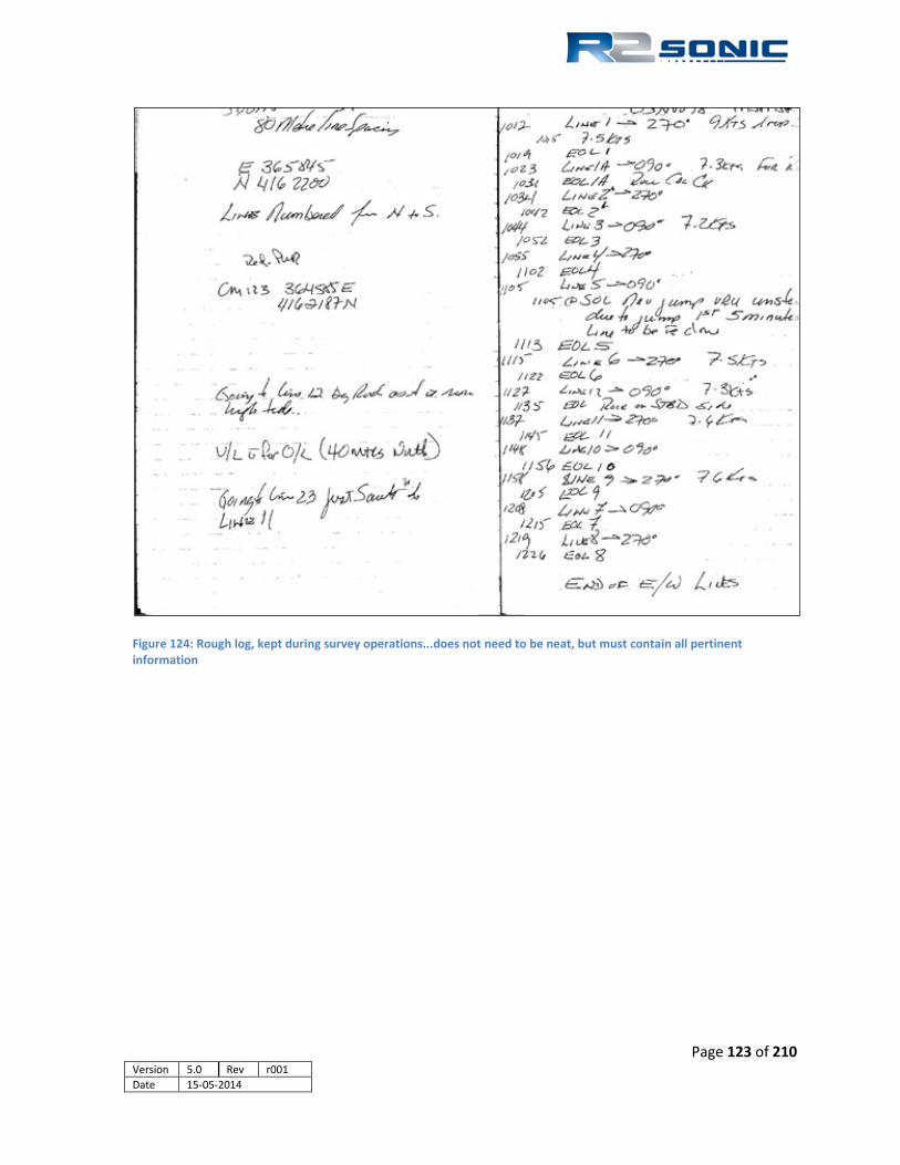
Figure 124: Rough log, kept during survey operations...does not need to be neat, but must contain all pertinent information


Figure 125: Smooth log; information copied from real-time survey log

APPENDIX IV: Offset Measurements

10 APPENDIX IV: Offset Measurements

10.1 Lever Arm Measurement – Offsets Each component or sensor that produces information, unique to its position, will have a point that is considered the reference point of that sensor. The Sonic 2024/2022, the motion sensor, and the GPS antenna will have a documented point from which to measure. The gyrocompass’ data is not dependent on its position on the vessel so, therefore, does not require an offset measurement.

10.2 Vessel Reference System When all equipment (Sonic 2024/2022 sonar head, motion sensor, gyrocompass and GPS) have been permanently mounted, the physical offsets to a central reference point (CRP) must be measured. The central reference point (CRP) or vessel reference point (VRP) is that point that the surveyor chooses to be the origin for the X and Y grid that will define the horizontal relationship between all of the sensors. The vertical or Z reference can be the water line or other logical vertical reference. Generally, the CRP corresponds to the centre of gravity or rotation of the vessel. All of the sensors must have their physical relationship to each other measured and entered into the data collection software or the processing software.

All offsets, between sensors, are defined by an X, Y and Z offset from a reference (CRP or VRP) point. The X axis runs athwartship, i.e. from the port side to the starboard side. The Y axis runs alongship from the bow to the stern. The Z axis runs perpendicular through the reference. The origin can be any point; the origin will remain the same for all sensors. Some surveyors take the GPS antenna as the origin for all measurements, others take the sonar head itself, while others might take the motion sensor (especially if it on the centre of rotation for the vessel). The sign convention is standard for a Cartesian plane, translated to a vessel: starboard of the reference point is positive, forward of the reference point is positive. The sign for Z may differ, depending on the data collection or processing software.

Page 125 of 210 Version 5.0 REV r001 Date 15-05-2014

Figure 126: Vessel Horizontal and Vertical reference system

10.3 Measuring Offsets The accurate measurement of offsets is vital to the accuracy of the survey data. If possible, the vessel will be put on a hard stand so that it can be very accurately measured using standard land survey equipment, such as a total station. However, this may not be possible and the offsets will have to be measured using a tape and plumb-bob, which is detailed below.

10.3.1 Sonic 2024 Acoustic Centre Please refer to the drawings appendix to obtain measurements, with reference to the system offsets, when mounting on the Sonic mounting frame.

Figure 127: Sonic 2024/2022 Acoustic Centre

10.3.2 Horizontal Measurement All measurements should be made with a metal tape measure. A cloth tape can stretch, it can also be knotted or kinked, unknown to the persons making the measurements. At a minimum, two people should be assigned to take the measurements; three people will work better with the third person writing down the measurements. One person will be the holder and the other will be the


reader. Starting at either the reference point or the sensor, the distance will be measured. When either the reference point or the sensor is reached, the two people will reverse roles: the holder is now the reader and the reader is the holder, the transverse is made back to the point of beginning, but not using the same path. If reference marks were made on the first leg, they should not be used on the second leg back. If the measurement from the sensor to the reference point, in one direction, agrees with the measurement in the opposite direction, made by a different reader and holder, then the offset is good. If there is a small disagreement in measurements, the two measurements can be averaged. If there is a large disagreement then the process should be repeated. What is a small disagreement? A few centimetres can be expected.

10.3.3 Vertical Measurement To measure elevations or the Z offset, the use of a plumb bob is required. This can be something as simple as a spanner tied to a length of line and lowered from one deck to the next. The plumb bob will also allow for accurate measurements in the X and Y direction when transposing them from one deck to the other.

The plumb bob works, of course, by gravity so generally points to the centre of the earth. This being the case, if the vessel is not in good trim, i.e. has a list, the resting position of the plumb bob may not be at the true vertical point under the place from which it is being held. This is very critical when transposing X and Y measurements from one deck to another.

The draft of a vessel will not be constant. Prior to going out on a survey, the fuel and water may be filled up, causing the vessel to settle lower in the water. Possibly less people are on board causing the vessel to rise higher in the water. The main concept here is that the draft of the sonar head changes. All X and Y offsets remain the same as long as the sensors are not moved, but the Z offset changes constantly depending on the draft of the vessel.

If possible, the pole should be marked to show the depth of the head. Measuring up from the sonar head’s acoustical reference, rings can be painted on the pole in 10 cm (or other) increments, with 2 cm hatching between rings. The surveyor may have to observe the pole over the course of a few minutes to determine where the water line is and would then estimate the depth by interpolating between the 10 cm depth rings.

Another method would be for the surveyor to initially measure from the sonar head’s acoustical reference to the top of the hydrophone pole. This is the total pole measurement. At the start of a survey day, the surveyor will go to the pole and measure from the top of the pole to the water line (using the tape measure and plumb bob or similar weight), this is called the dry measurement. Taking the dry measurement from the total pole measurement yields the wet measurement, which is the draft of the sonar head. Due to wave motion, the surveyor may have to take a series of measurements to ensure an accurate reading.

When the draft or Z of the sonar head is determined the Z for the GPS antenna and the motion sensor can be adjusted accordingly, if the Z reference is the water line. In most data collection software a Z shift, in relation to the water surface, can be entered in for the CRP, which will do the vertical adjustment for all offsets

It is very important that when measuring the draft on small vessels that the person taking the measurement does not unduly cause the vessel to list towards that side. Having someone counter


balance the weight of the person taking the measurement is a good idea. This is also true of any temporary list the vessel is experiencing. On small survey vessels, a person leaning over the side, to take the draft measurement, can induce upwards, or exceeding a 10cm error in depth readings during survey operation.

On some vessels it is advisable to take draft readings during the survey or immediately after completion of the survey, as the draft will change that much.

All offset information should be recorded in the daily survey log and the vessel’s permanent survey record.


APPENDIX V: The Patch Test

11 APPENDIX V: The Patch Test

11.1 Introduction The alignment of the Sonic 2024/2022 sonar head to the motion sensor and gyro is critical to the accuracy of the determined depths. It is not possible to install the sonar head in exact alignment with the motion sensor and gyro to the accuracy required (x.xx°). If GPS time synchronization is not used, the latency of the position, as reported by the GPS, must also be measured during the calibration. This being the case a multibeam calibration must be performed to measure the angular misalignment between the Sonic 2024/2022 and the motion sensor and gyro and, if necessary, the position latency; this is called the Patch Test. The patch test is performed with each new installation or whenever a sensor is moved. In the case of an over-the-side mount, a large number of calibration computations need to be performed to determine how well the pole goes back into the same position each time it is deployed. With more permanent mounting arrangements, a minimum of 5 separate patch tests should be conducted in order to derive a standard deviation that would indicate the accuracy of the derived values.

The patch test involves collecting data over certain types of bottom terrain and processing the data through a set of patch test tools. There are two primary methods of processing the data that are currently used: an interactive graphical approach and an automatic, iterative surface match. Each of these techniques has strengths and weaknesses and the preferred approach is dependent on the types of terrain features available to the surveyor. All modern multibeam data collection software packages contain a patch test routine. Please read the software manual for explicit information regarding the requirements for that software’s patch test. The below criteria is, in general, the norm for a patch test.

11.2 Orientation of the Sonic 2024/2022 Sonar Head The orientation of the sonar head must be known in order to convert the measured slant ranges to depths and to determine the position of each of the determined depths.

Any error in the measured roll of the Sonic 2024/2022 sonar head can cause substantial errors in the conversion from slant range to depth. A roll error of 1° on a 50 m slant range will cause a 0.6 m

error in the resulting depth. Any error in the measured pitch of the Sonic

2024/2022 head will primarily have a detrimental effect on the accuracy of the positions that are determined for each slant range/depth.

A pitch error of 1° will cause an along-track error in the position of 0.4 meter when the sonar head is 25 meters above the seabed.

Figure 128: Sonic 2024/2022 axes of rotation


11.3 Patch Test Criteria The patch test requires collecting sounding data over two distinct types of sea floor topography; a flat bottom is used for the roll computation whereas a steep slope or feature is used for the latency, pitch, and yaw data collection.

Care must be taken that the sonar head covers the same area on both data collection runs, this may not be the same as vessel position, especially with an over-the-side mount or if the sonar head rotated. Only the latency data collection requires a different speed from normal survey speed.

The data collection for Latency, Pitch and Yaw should be done in as deep water as possible. This is particularly true for the pitch computation due to the fact that in shallow water the angle of pitch may not be easily determined due to a lack of resolution.

11.3.1 Latency Test The vast majority of installations will incorporate GPS time synchronisation and, as such, no latency is expected in the GPS position. However, it is necessary to complete at least one or two latency tests to prove that the latency, for all practical purposes, is zero. Most patch test programs will not yield zero latency, but the derived value would be so small so as to constitute a practical zero.

For the latency test, data is collected on a pre-defined line up a steep slope or over a well-defined object (such as a rock or small wreck). The line is surveyed at survey speed up the slope, and then surveyed again, in the same direction, but at a speed that should be half of the survey speed. If the vessel cannot make way at half survey speed then the fast run will need to be taken at a higher speed than normal survey speed and this can influence the latency test due to squat or settlement. The main consideration is that one line should be twice the speed of the other.

Figure 129: Latency Data collection


11.3.2 Roll Test The data collection for roll has to be over a flat sea floor. One line is surveyed twice, in reciprocal directions and at survey speed.

When the data, from the two data collections, are looked at in profile, there will be two seafloors sloped in opposite directions. Most patch test programs will go through a series of iterations to determine when the difference between the two surfaces is the smallest, and this is the roll offset.

Figure 131: Roll data collections

Roll is perhaps the most critical value in the patch test routine as an error in roll will result in an error in sounding depths.

However, the computation to determine the roll misalignment is usually the easiest and most consistent.

Graph 1: Depth errors due to incorrect roll alignment

-0.60

-0.40

-0.20

0.00

0.20

0.40

0.60

-80 -60 -40 -20 0 20 40 60 80

Sounding Error due to +0.5° Roll Error in 20 metres depth

Degrees from Nadir

Dept

h Er

ror i

n M

etre

s

Figure 130: Roll data collection


11.3.3 Pitch Test The pitch data collection is over the same type of sea floor as the latency data collection, i.e. steep slope or feature on the sea floor. One line is surveyed, twice, in reciprocal directions at survey speed. It is very critical that the sonar head passes over the same exact part of the slope on each run.

A profile of the data will show two different slopes, which represent the reciprocal data collections. The patch test software goes through a series of iterations of pitch angle corrections until the difference between the two surfaces reaches a null. Whatever the angle of correction, which results in the minima or null, that angle will be reported as the pitch misalignment.

A pitch error will result in a an along –track position error, which increases greatly with depth

Graph 2: Position errors as a result of pitch misalignment; error can be either negative or positive

0

1

2

3

4

5

6

0 100 200 300 400

Soun

ding

Pos

ition

Err

or (m

etre

s)

Water Depth (metres)

Position Errors due to Pitch Alignment Errors

1.0° Error

0.75° Error

0.5° Error

0.25° Error

Figure 132: Pitch data collections


11.3.4 Yaw Test The yaw data collection and subsequent solving for the yaw offset is usually the most difficult of the 4 tests that comprise a patch test. This is especially true if a slope is used for the yaw computation; a feature generally works much better. The reason for this is that the area that is used for the computation is not directly under the vessel, but in the outer beams and the slope may not be perfectly perpendicular in relation to the course of the vessel.

For the Yaw data collection two parallel lines are used, with the vessel surveying in the same direction on those lines. The lines are to be on either side of a sea floor feature or over a slope. The lines should be approximately 2 – 3 times water depth in separation. A yaw error will result in a depth position error, which increase with the distance away from nadir.

Graph 3: Along track position error caused by 0.5° error in yaw patch test

-6

-4

-2

0

2

4

6

-80 -60 -40 -20 0 20 40 60 80

Alon

g-tr

ack

Posi

tion

Erro

r in

Met

res

Angle from Nadir

Position Error with a Heading Error of 0.50°

200 metres

150 metres

100metre

50 metre

25 metres

10 metres

Water Depth

Figure 133: Yaw data collection


Graph 4: Along-track position error caused by 1.0° error in yaw patch test error

11.4 Solving for the Patch Test Depending on the data collection software that is employed and how it solves for the patch test, there will be a distinct order that the tests will be solved for, but this does not influence the data collection for the patch test. In general, latency will be solved before pitch; roll will be solved for before yaw. It is not uncommon that a larger than expected error in one of the tests will make it necessary to go back and resolve for all previous values. This can be the case with a large yaw offset, as this will influence to a greater degree the accuracy of the latency and pitch computations if done using a slope.

The resultant patch test values are corrections that are entered in the data collection software and not in the Sonic 2024/2022 software, as the values are used for process data.

11.5 History Since the advent of commercial multibeam echosounders there has been the need to measure the angular offsets between the multibeam sonar head and the auxiliary sensors that provide attitude and heading information. Another measurement is made to determine the latency, in the GPS receiver. Multibeam data is collected that is used to determine (1) latency, (2) roll offset, (3) pitch offset and (4) heading or yaw offset

What has been developed is called the Patch Test; this is the multibeam calibration. During the development of the data collection criteria, for the Patch Test, there has only been a basic description for the manner of the data collection; providing little, if any, directions that would help create a high degree of confidence in the results of the various tests. This section will

-10

-8

-6

-4

-2

0

2

4

6

8

10

-100 -50 0 50 100

Alon

g-tr

ack

Posi

tion

Erro

r in

Met

res

Angle from Nadir

Position Error with a Heading Error of 1.0°

200 metres

150 metres

100metre

50 metre

25 metres

10 metres

Water Depth


address those very directions that will help create a highly accurate and statistically viable result from the Patch Test.

11.6 Basic data collection criteria Patch test data collection does not have to be in any set order, but the order that the values are computed, in the data collection or processing software, will be in a distinct order. Normally, Latency is the first value that is computed, followed by Roll, Pitch and Yaw (or heading). The solving order is important, as will be seen below.

11.7 Patch Test data collection error areas There are many common errors, or mistakes, made during the patch test data collection.

11.7.1 Positioning The accuracy of the positioning system is a common area where errors arise. DGPS has, at best, a variability of ± 0.50 metres, whereas RTK variability is ±0.05metres. A recent article, by Mike Brissette, (MosaicHydro LTD, Canada) in Hydro International (‘Stop Using DGPS’; Hydro International; Volume 16, Issue 7; Oct 2012) documents this issue very well: http://www.mosaichydro.com/papers/M%20Brissette%20-%20Stop%20Using%20DGPS.pdf The article fully details the errors that can occur by using DGPS, instead of highly accurate positioning for the Patch Test data collection. The error increases inversely with the water depth, i.e. the shallower the water, the larger the error that can be induced by using DGPS over more accurate positioning. However, many users do not have any better positioning capabilities than DGPS; how can they still obtain valid patch test results without having centimetric accurate positioning? This is, in large part, what this paper is concerned with. However, even with centimetric position, the following should be followed.

11.7.2 Feature chosen for test Where at all possible, for latency, pitch and heading data collection, a feature should be used rather than a slope. Slopes tend to be too variable as opposed to a well-defined feature such as a wreck, rock outcrop or pipeline. One of the other issues, with using a slope, is that many times the shallow end of the slope does not allow sufficient area or depth for the vessel to come about and line up for the reciprocal run; this does not allow sufficient time for the motion sensor to settle down nor for the helmsman to find a steady course. It has been found that when using a slope, for the pitch calibration, that the heading angular offset can have a large influence. If the sonar head does not track exactly the same route, up and down the slope, the heading offset will affect the pitch angular result.


http://www.mosaichydro.com/papers/M%20Brissette

11.7.3 Water depth The deeper the water, the better the result. In shallow water, DGPS wobble (as noted in the Brissette paper), creates more relatively severe position errors. A corollary to this is that the subtended angle is larger in shallow water, which can blur the definition of the object used, be it a feature or slope. The shallower the water, the larger the subtended angle; the deeper the water, the smaller the subtended angle and, therefore, the better the definition of the object or slope.

11.7.4 Use predefined survey lines The most important positioning issue is having the sonar head pass over the same exact location in both of the survey data collections. This is especially true when using a highly variable slope. One way to assist the helmsman is to give the helmsman a defined line to navigate by. Just trying to go over the same track, without a line reference, does not work, as it is the sonar head that has to pass over the same exact point; this accuracy cannot be obtained just by using the grid display to steer the vessel. When setting up the survey software, make sure that the sonar head is the steered reference for all offline measurements. It does no good to have the vessel on the survey line, if the sonar is mounted on the side of the vessel; it is the sonar that should be on the survey line.

11.7.5 Speed When doing the latency data collection, the fast run should be at survey speed where, if there is squat or settlement, it should have been previously measured and can be applied. Many times, the fast run survey line is at a speed that is greater than the normal survey speed and induces unknown squat and settlement errors into the computation.

11.7.6 Vessel line up In order for the angular measurement to be accurate, the vessel should have sufficient time to come on line and allow the motion sensor to ‘settle down’. Sufficient lead/run in should also be allowed in order for the helmsman to find the proper heading so that vessel can maintain as straight a course as possible.

11.7.7 Pole variability The other issue, which is often overlooked, is the variability in the repeat position of a deployable hydrophone pole. With any moveable mounting arrangement the pole should be recovered and redeployed a few times, during data collection, to determine if it does, indeed, go back into the same aspect every time that it is deployed. (It is a good idea, after redeploying the head, to do a few figure 8 manoeuvres.)


11.8 Improving the Patch Test and Patch Test results Section 11.7 described areas that should be addressed to improve the results of the patch test when collecting the data. Further improvement will come with the number of data collections and the manner in which the patch test is computed.

11.8.1 Need to collect sufficient data Too many times, surveyors will collect just a few lines of data for each test. One of the major issues, detailed above, is the variability of the position accuracy of DGPS. Another issue, detailed above, is the steering of the vessel during the data collection and the relationship of the sonar head to the feature or slope on each data collection.

In order to overcome the variability of the DGPS positioning and vessel steering, it follows that the more tests that are performed, the greater will be the reliability of the test results. Below, is an example of a multibeam calibration, which included five data collections for each test.

ROLL PITCH YAW

0.73 -0.73 1.02

0.73 -0.99 0.90 0.76 -2.16 0.81 0.76 -1.07 2.26

0.74 -0.83 0.94

Pitch mean with erroneous value = -1.16 (SD = 0.58); without erroneous value of -2.16 = -0.91 (SD = 0.13) Yaw mean with erroneous value = 1.19 (SD = 0.61); without erroneous value of 2.26 = 0.92 (SD = 0.08)

Consider the above patch test and what the result would have been if only two collections were made and those were the ones that contained the highlighted values, which can clearly be seen to be outside of the trend. Having more data to work with, a more reliable result can be achieved.

The more data collected, the more evident will be any out of trend values that may reflect a DGPS wobble, a steering issue, or variability of the positioning of the pole. Enough data should be collected to provide a reliable statistical result, i.e. mean and standard deviation. Collecting enough data to compute six of each test, allows the exclusion of any one ‘out of trend’ result to yield a mean and standard deviation derived from five computations; this would be a statistically viable sampling.


11.8.2 Individually solving values No matter what the solving order may be, each value should be computed independently. All tests should be based on the mean of the previous test(s). It is important to understand why a certain solving order is used in all survey software. Each computation is based on the previous test result. This is the reason that latency is computed before pitch and roll is computed before heading; the primary test (latency or roll) has a large influence on the result for the secondary test (pitch and heading). The roll computation can also have an influence on the pitch computation, primarily if the position of the sonar head, of the reciprocal runs, was not coincident. The heading offset will also have an influence on the pitch computation for the same reason. Generally, multibeam surveys are conducted with very accurate time synchronisation using GPS time and the Pulse Per Second. In this case, the latency test is used to prove the lack of latency or that is sufficiently small enough so as to be of no consequence. Using accurate timing, it is not necessary to collect more than two latency collections. This paper will concentrate on the angular offset computations. However, if accurate timing is not used there should be the same number of collections as with the other tests. With a good number of individual tests, solve for one computation (i.e. only roll) and derive a mean and standard deviation for that one test. Determine if the standard deviation is within acceptable accuracy requirements, then use that derived mean to solve for the next computation (i.e. pitch). As an example, using the results on page 7, the first step would be to solve for Roll first, derive a Roll mean and then use that mean in all of the Pitch computations. Find the mean and standard deviation for Pitch. Use the mean Roll and Pitch values to determine the Heading offset. In the above example, the roll mean, of the five tests, is 0.74°, with a standard deviation (δ) of 0.01°. The roll mean would now be used when determining the value for pitch. Use the roll mean and solve all of the pitch computations; the pitch mean is -0.91° (excluding the out of norm value), δ = 0.13°. The roll and pitch computed means are now used to solve for the heading offset. The solved heading offset is 0.92°, δ = 0.08°. If the heading offset had been 1.5° or greater, it would be advisable to re-compute the pitch offset, using the computed heading offset value. This is due, again, to the fact that if the sonar head did not track the same exact position in the reciprocal runs, the heading offset will have an influence on the pitch offset result.

11.9 Truthing the patch test After deriving the values for roll, pitch and yaw, the values should be entered into the appropriate areas in the data collection software. Ideally, find a singular object that can be boxed in (running data collection lines, on all sides of the object) and process the data. The object depiction, with all survey lines, should not vary from the object depiction from any one line.


APPENDIX VI: Basic Acoustic Theory

Figure 134: In 1822 Daniel Colloden used an underwater bell to calculate the speed of sound under water in Lake Geneva, Switzerland at 1435 m/Sec, which is very close to recent measurements.

12 APPENDIX VI: Basic Acoustic Theory

12.1 Introduction With multibeam, as with any echosounder, a main concern is: sound in water. Once the projector transmits the acoustic energy into the water, many factors influence that energy’s velocity and coherence. The major influence is the velocity of sound in water.

12.2 Sound Velocity The major influence on the propagation of acoustic energy is the sound velocity of the water column. As the acoustic pulse passes through the water column, the velocity and direction (refraction) of the wave front will vary based on the water column sound velocity. If the sound velocity, through the water column, is not accounted for in the data collection software the depths and the depth location will be in error. For this reason, sound velocity casts are an oft repeated routine during multibeam survey.


Figure 135: Concept of refraction due to different sound velocities in the water column

The velocity of sound in water varies both horizontally and vertically. It cannot be assumed that the velocity of sound in the water column remains constant over large areas or throughout the day in a more local area. The main influences on sound velocity are: Conductivity (salinity), Temperature and Depth (pressure).

1 ° C change in Temperature = 4.0 m/sec change in velocity 1 ppt change in Salinity = 1.4 m/sec change in velocity

100 m change in Depth (10 atm’s pressure) = 1.7 m/sec change in velocity

Figure 136: Sound velocity profile


12.2.1 Salinity Generally, salinity ranges from 32 – 38 parts per thousand (ppt) in ocean water. A change in salinity will create density changes, which affect the velocity of sound. As a general rule, a change in salinity of only 1 ppt can cause a sound velocity change of 1.4m/sec. There are many influences on the salinity concentration in sea water.

1. Evaporation 2. Precipitation 3. Fresh water influx from rivers 4. Tidal effects (salt wedges)

12.2.2 Temperature Temperature is the major influence on sound velocity in water. A 1°C change is equal to approximately a 4m/sec change in velocity. Once the upper layer is passed, the temperature normally decreases until pressure becomes the more dominating influence on the velocity of sound, which is approximately at 1000 metres. The normal influences on the temperature component of sound velocity include:

1. Solar heating 2. Night time cooling 3. Rain / run off 4. Upwelling

12.2.3 Refraction Errors Refraction errors occur due to the wrong sound velocity profile being applied to the data. The error increases away from nadir and, as such, is more apparent in the outer beams. The visual effect is that the swath will curl up (smile) or curl down (frown). The actual representation is that the soundings are either too shallow or too deep.

Figure 137: Refraction Error indication

At an angle of 45° in 10 meters of water, a ±10 meters per second velocity error will result in a depth error on the order of ± 4.6 cm.

• Convex (smiley face) = Sound velocity profile used higher than real profile • Concave (frown face) = Sound velocity profile used lower than real profile


12.3 Transmission Losses The transmission of an acoustic pulse is generally called a ‘ping’. When the projector sends out the acoustic pulse many factors operate on that pulse as it moves through the water column to the bottom and also on its return upward. The major influence of the water column sound velocity characteristics was detailed above; this affects the speed of transmission (and return). There are other influences that will affect acoustic energy in water and these are transmission losses.

12.3.1 Spreading Loss Spreading loss does not represent a loss of energy, but refers to fact that the propagation of the acoustic pulse is such that the energy is simply spread over a progressively larger surface area, thus reducing its density. Spreading loss is not frequency dependent.

12.3.1.1 Spherical Spreading Spherical spreading loss is the decrease in the source level if there are no boundaries (such as the water surface or sea floor) to influence the acoustic energy; all of the acoustic energy spreads out evenly, in all directions, from the source. The loss in intensity is proportional to the surface area of the sphere. The intensity decreases as the inverse square of the range for spherical spreading. With Spherical spreading, the transmission loss is given as: TL = 20log(R), where R is range

Figure 138: Concept of Spherical Spreading

12.3.1.2 Cylindrical Spreading In reality the acoustic energy cannot propagate in all directions due to boundaries such as the sea floor and the water surface; this give rise to Cylindrical Spreading. Cylindrical spreading is when the acoustic energy encounters upper and lower boundaries and is ‘trapped’ within these boundaries; the sound energy begins to radiate more horizontally away from the source. With Cylindrical spreading the acoustic energy level decreases more slowly than with Spherical spreading. With Cylindrical spreading, the transmission loss is given as: TL = 10log(R), where R is range.

Point Source of Acoustic Energy


Figure 139: Concept of Cylindrical Spreading

12.3.2 Absorption Absorption is frequency dependent and refers to the conversion of acoustic energy to heat when it strikes chemically distinct molecules in the water column. Magnesium Sulphate MgSO4

predominates, with Boric Acid B(OH)3 playing a major part at lower frequencies. Temperature is also an influence on absorption. Absorption is one of the key factors in the attenuation of the acoustic energy based on frequency; the higher the frequency, the greater the absorption. The higher the sonar operating frequency, the more rapid the vibration (or excitement) of the particles in the water and this leads to the greater transference of acoustic energy; thus, the attenuation of the acoustic wave. This is the reason why lower frequencies are used to obtain deeper data. At 400 kHz, the normal seawater absorption is approximately 100 dB/km, whereas at 200kHz the absorption is approximately 50 dB/km. These are values for normal sea water (with a salinity of 35 ppt). Fresh water has little, if any salinity (<0.5ppt), so absorption is considerably less.


The below table and charts illustrate how frequency, water temperature, and salinity affect absorption

Seawater Absorption Values: Salinity = 35ppt, pH=83 dB/km

400kHz

200kHz Temp (C) 5° 10° 15° 20° 25°

5° 10° 15° 20° 25°

Depth (m) 50 97 100 111 130 154

46 56 68 80 89

100 96 100 110 128 153

46 55 67 79 88 150 96 99 110 128 152

46 55 66 78 88

200 95 99 109 127 151

45 55 66 78 87 250 95 98 109 126 150

45 54 66 77 86

300 95 98 108 125 149

45 54 65 77 86

400m 44 53 64 76 84

Mean Value 96 99 110 127 152 45 55 66 78 87

Freshwater Absorption Values: Salinity = 0.5ppt, pH=7 dB/km

400kHz

200kHz Temp (C) 5° 10° 15° 20° 25°

5° 10° 15° 20° 25°

Depth (m) 50 65 55 46 39 33

17 14 12 10 9

100 65 54 46 38 33

17 14 12 10 9 150 65 54 45 38 33

17 14 12 10 9

200 65 54 45 38 32

17 14 12 10 9 250 65 54 45 38 32

16 14 12 10 9

300 64 54 45 38 32

16 14 12 10 9

Mean Value 65 54 45 38 33 17 14 12 10 9 Table 12: Absorption Values for Seawater and Freshwater at 400 kHz and 200 kHz

3 Equation used for computation is from: Ainslie M.A., McColm J.G., “A simplified formula for viscous and chemical absorption in sea water”, Journal of the Acoustic Society of America, 103(3), 1671-1672 as employed on the NPL website, op cit. Page 144 of 210 Version 5.0 Rev r001 Date 15-05-2014 Part No. 96000001

Graph 5: Seawater Absorption (Salinity 35ppt)

Graph 6: Freshwater Absorption

0

20

40

60

80

100

120

140

160

5° 10° 15° 20° 25°

Abso

rptio

n dB

/km

Frequency and Temperature Influence on Seawater

Absorption

400kHz

200kHz

Degrees Celsuis

Mean values for water depths from 50 metres to 300 metres (400 metres for 200 kHz)

0

10

20

30

40

50

60

70

5° 10° 15° 20° 25°

Abso

rptio

n dB

/km

Frequency and Temperature Influence on Freshwater Absorption

400 kHz

200 kHz

Degrees Celsius

Mean values for water depths from 50 metres to 300 metres

(


Seawater Absorption dB/km

Freq. 10°C 15°C 20°C 25°C 30°C

200 55 67 80 89 92

210 57 69 82 94 98

220 59 71 85 97 104

230 61 74 88 101 109

240 63 76 91 105 115

250 65 78 94 109 120

260 67 80 96 113 125

270 69 82 99 116 130

280 71 84 101 120 134

290 73 86 104 123 139

300 75 88 106 126 143

310 78 91 108 129 148

320 80 93 111 132 152

330 82 95 113 135 156

340 85 97 115 138 160

350 87 99 118 141 164

360 90 102 120 143 168

370 92 104 122 146 171

380 95 106 125 149 175

390 98 109 127 152 179

400 100 111 129 154 182

700 213 2074 214 235 270

Table 13: Operating Frequency - water temperature - absorption

4 At 700 kHz, there is an absorption dip, in this temperature range Page 146 of 210 Version 5.0 Rev r001 Date 15-05-2014 Part No. 96000001

12.3.3 Reverberation and Scattering The sea is not homogenous in nature. Everything from suspended dust particles to fish, from the sea surface to the sea floor will scatter, that is reradiate, the acoustic energy. All of the effects of individual scattering can be termed reverberation. The effect of reverberation is to lessen the acoustic energy and this leads to transmission losses.

Reverberation is divided into three main areas: sea surface reverberation, bottom reverberation, and volume reverberation (the body of water that the energy is passing through).

Both the sea surface and the sea bottom will reflect and scatter sound, thus affecting the propagation of sound. Sea surface scattering is influenced by how rough the sea is (which is related to wind velocity) and also the trapped air bubbles in the near surface region. The sea surface is also a good reflector of acoustic energy; this can lead to second and even tertiary bottom returns as the bottom return acoustic energy is reflected by the sea surface and is then reflected once more by the sea bottom.

In the case of the sea floor, the strength of the scattering depends on the type of bottom (composition and roughness), the grazing angle of the acoustic pulse and the operating frequency of the sonar.

There is also bottom absorption based on the sea floor terrain and composition. Bottom absorption is also dependent on the operating frequency of the sonar and the angle of incidence. Bottom absorption will be greater for a higher frequency and large angle of incidence. It is more or less intuitive that a mud bottom will absorb more of the acoustic energy than a rocky bottom. When the acoustic energy is absorbed it means there is less that will be reflected back to the Sonic 2024/2022’s receivers. The surveyor must be aware of the bottom composition as adjustments can be made to the Sonic 2024/2022 operating parameters to help compensate for the bottom absorption.

In waters with a large sediment load, the suspended particles will scatter the sound wave, thus leading to transmission loss. In the scattering process, there is also a degree of energy that it is reflected (backscatter); this can be a cause for ‘noise’ in the sonar data. Again, the surveyor should be aware of this condition and, if need be, change the operating parameters of the Sonic 2024/2022. When discussing the changing of the operating parameters, it is generally a matter of increasing transmit power or pulse length to get more total power into the water. In some circumstances, increasing the Absorption value will allow the system to rapidly increase gain to capture the reflected energy that has been dissipated by seafloor absorption or scattering in the water column.

As noted above many of the effects of absorption, scattering, and bottom absorption are frequency dependent. With the Sonic 2024/2022, the operator can adjust the sonar frequency to optimise the system for the survey conditions. This will take some trial and error; however, lower frequencies tend to do best in areas of absorbent bottom and high sediment load (scatter).



Appendix VII ROV and AUV Installation

13 APPENDIX VII: Sonic 2024/2022 Mounting: Sub-Surface (ROV/AUV)

13.1 Installation Considerations • A 1000BASE-T link (best time sync accuracy) is preferred; however, with bathymetry only

information, 100BASE-T will work. 10BASE-T will also work, but is not recommended. Bathy data requires 2 Mb/s data rate at a maximum ping rate of 60 pings/sec. For future compatibility, please use 100BASE-T at minimum, Snippets will not work with 10BASE-T; however, Snippets will work over a 100BASE-T link.

• Average power, for a Sonic 2024 is 50W (1A), peak is 100W (2A); for a Sonic 2022 it is 35W (0.73A), peak is 75W (1.5A). The peak power of 100W (75W) occurs just after transmit and typically lasts for a few msecs (depends on transmitter power setting). If you use a separate power supply for the sonar, we recommend using a 120 to 150W power source to supply the head, but less if installing a Sonic 2022.

• The sonar up/down link is all done through the Ethernet channel. Thus, no other hardware is required except for the Ethernet media converters (copper to fibre, fibre to copper). As a precaution, placing additional filtering on the output of the 48V supply to the sonar head is a good idea to prevent vehicle electronic noise from getting into the sonar head. A common mode choke, on the 48V line, is recommended. The Bourns (JW Miller) PM3700-50-RC common mode choke works well (surface mount part). A Bourns 8102-RC choke, which is easier to install (non-surface mount) can also be used.

• The supplied deck cable is a special cable with Ethernet pairs which are rated to 3000 meters water depth. Do not substitute this cable, as the Ethernet data pairs need to meet certain important specifications. When terminating the Ethernet connections to your own connector, the Ethernet twisted pairs need to terminate right at the connector pins, maintaining the twist on the wires as close to the connector pins as possible. On the bulkhead connector, use CAT5, or better Ethernet cable, from the connector, to the Ethernet media converter. Use adjacent pins for each wire pair. If 100BASE (or 10BASE) Ethernet is used, only the green and orange pairs are required. All four pairs, including blue and brown, are only required when using gigabit Ethernet.

• Using a connector with a pigtail spliced on to the deck leads’ Ethernet pairs has a low probability of working. If the deck lead must be terminated to a pigtail, the pigtail length must be as short as possible, probably no more than 7-8cm. There are no special considerations for the power conductors other than the connector being able to handle 48VDC and 2 amperes. The drain (shield) wire does not need to be terminated.


13.1.1 Ethernet wiring considerations The sonar head and SIM use gigabit Ethernet ports. There are rules, regarding number of pairs of wire to use, between different Ethernet ports, those rules are:

• Gigabit to Gigabit

Need all four pairs. If only two pairs used, in an attempt to force the ports to 100BASE-T, the ports will not negotiate and the result will be no connection. (As of the 16Nov2013 head firmware, two pairs can be used; this will put the head in a 100BASE-T connection.) Sometimes it's not obvious if a port is Gigabit enabled; the Status display shows the Ethernet connection speed for the head. This is useful for troubleshooting connection issues.

• Gigabit to 100BASE-T

Two pairs (green and orange on TIA/EIA-568-B wiring) can be used. Be sure to test this with a modified patch cable (cut the brown and blue pairs) before committing to the chosen Ethernet equipment as there may be surprises hidden in the equipment.

• 100BASE-T to 100BASE-T: You can use two pairs (green and orange, T568B).

When connecting to the SIM, use either of the AUX Ethernet ports for the sonar head Ethernet connection.

13.2 Data Rates Bathy: ≈800 kb/s max (bathy data is sent twice, to GUI and data acquisition computer) Snippets: ≈11Mb/s max TruePix™: ≈ 5.5 Mb/s (magnitude +angle) max ≈ 3.5 Mb/s (magnitude) max Water Column: ≈280 Mb/s max for magnitude only ≈560 Mb/s max for magnitude + phase AI(FLS): Depends on GUI wedge size; more information will be added The data rate, for water column data, can be significantly reduced by increasing the pulse width. At certain pulse widths, the receiver sampling rate halves, which will make the water column data rate halve. As an example: Pulse width 15µsec - 30µsec: 65 kHz sample rate = Ethernet: 35 Mb/sec (amplitude) 280 Mb/s

(amplitude and phase) Pulse width 35µsec - 70µsec: 32.5 kHz sample rate = Ethernet: 17.5 Mb/s (amplitude), 140 Mb/s

(amplitude and phase)


13.3 ROV Installation Examples

Figure 140: Single Head ROV Installation scheme A

Figure 141: Single Head ROV Installation scheme B (Preferred)


Figure 142: Dual Head ROV Installation scheme A

Figure 143: Dual Head ROV Installation scheme B (Preferred)


13.4 Power Requirements The basic over the side installation of the Sonic 2022 and 2024 systems consists of the sonar head, projector, SIM box, sound velocity probe, and interconnecting cables. The sonar head, SIM, and computer(s) communicate via 100BASE-T or 1000BASE-T (Gigabit) full duplex Ethernet.

Installation in an ROV requires an Ethernet media converter to convert copper to fibre optic and back to copper media to accommodate long tethers. On shorter ROV tethers (less than 1000 metres), using impedance controlled twisted-pair copper wire and a DSL modem may be possible.

Remote or autonomous vehicles typically supply the 48 volt power to the sonar head, and if required, the SIM Controller board.

Device Power Conditions 2024 with SIM 95 to 260VAC, 75 W 2024 head connected to SIM, equivalent to

over the side installation. Conditions: 30m range, Tx power = 215 dB, pulse width = 50us.

2022 with SIM 95 to 260VAC, 54 W 2022 head connected to SIM, equivalent to over the side installation. Conditions: 30m range, Tx power = 215 dB, pulse width = 50us.

SIM 95 to 260VAC, 16.5 W No connections to SIM 2024 head at 48V

1.05 A average 1.77 A peak after transmit

30m range, Tx power = 215 dB, pulse width = 50us.

2022 head at 48V 0.70 A average 1.34 A peak

30m range, Tx power = 215 dB, pulse width = 50us.

SIM control board

48V, 78mA (gigabit) 48V, 51mA (100BASE-T)

No connections except Ethernet.

Table 14: Systems Power Requirements

In an ROV or AUV installation, the sonar head and SIM Controller board require 48VDC which is supplied by the vehicle power system. The average power required is 50 watts for the 2024, 35 watts for the 2022. Just after transmit, an additional 50 watts is required to charge the transmit capacitor bank for a brief period of time. See below figures for current waveforms. If a separate power supply for the sonar is required, it should be rated for 120 to 150 watts or higher.


Figure 144: Sonic 2024 power supply current waveform. Peak current is 1.770A at 48V. Sonar settings: pulse width = 100us, Tx Power = 221dB, Freq = 400 kHz.

Figure 145: Sonic 2022 power supply current waveform. Peak current is 1.340A at 48V. Sonar setting: pulse width = 100us, Tx Power = 221dB, Freq = 400 kHz.

Figure 146: Inrush current to 2024 head during power up, 20 ms window.


Figure 147: Inrush current to the 2024 head during power up, 1 second window.

13.4.1 Common mode noise rejection Common mode noise on the 48VDC power line to the sonar head should be minimized. The SIM Controller board has a common mode choke on the power line to the sonar head. If sonar head power is not supplied by the SIM Controller board, install a common mode choke on the sonar head 48VDC power line. A suitable common mode choke is JW Miller (Bourns) 8102-RC. This is available from Digi-Key. See below figure for wiring details.

Figure 148: Power supply choke installation on 48VDC power


13.4.2 SIM Power connections

Figure 149: SIM Controller Power Connections

Figure 150: J6 Connector on SIM Controller board

The mating connector for J4: Molex 43645-0800 (8-way Micro-FIT 3.0) Molex 43030-0009 (socket contacts) Molex 63819-0000 or 63811-2800 (crimping tool for socket contacts) The mating connector for J6: Amp 2-111623-4 Any 2mm 2x20 header connector may be used for this part. 1mm pitch ribbon cable is also required


13.5 SIM Installation – ROV The SIM can be installed either top-side or in the vehicle. There are advantages to both methods which depend on the multiplexer capabilities. For SIM installation in the vehicle, the SIM Controller board may be removed from the SIM or supplied as an additional item. The SIM controller board uses a PC/104 size format, but does not use the PC/104 bus.

Figure 151: ROV installation block diagram with the SIM top-side

Figure 152: ROV installation block diagram with the SIM controller board mounted in the vehicle electronics bottle and GPS (ZDA or UTC formats) and PPS signals are supplied by top-side equipment

Figure 153: ROV installation block diagram with the SIM controller board mounted in the vehicle electronics bottle. GPS (ZDA or UTC formats) and PPS signals are supplied by the vehicle time system.


13.6 SIM Installation – AUV The circuit boards, inside the SIM, can be supplied separately as shown in Fig 133. The three boards use a PC/104 size format, but does not use the PC/104 bus. The three boards are the I/O board where the customer connects time, motion and sound velocity sensors; SIM Controller board; and a gigabit Ethernet switch.

It’s best that the SIM Controller board supply power to the sonar head as the controller board has a common mode choke for the 48 VDC power to the sonar head and the SIM Controller board can control power to sonar head. If the customer uses their own custom data acquisition software, a list of commands for the sonar head and SIM are in Appendix VIII. The uplink data format is provided in Appendix IX.

Figure 154: Typical wiring. GPS (ZDA or UTC formats) and PPS signals are supplied by the vehicle time system

Figure 155: SIM Board Stack

Figure 156: SIM Stack height

SIM board stacks: Top board: I/O Middle board: SIM controller Bottom board: Gigabit, 5-Port, Ethernet switch BNC connector: GPS PPS input SMB connectors: sync in and out


13.7 SIM Board Physical Installation 1. Power requirements: 48VDC, 50 watts average, 100 watts peak.

2. 36VDC is absolute minimum working voltage; 52VDC is absolute maximum working voltage

3. All boards are static sensitive. People handling the boards should be properly grounded.

4. User has the option to use the I/O board or not. The I/O board is connected to the SIM Controller Board via a ribbon connector (SIM Controller J6 and I/O board J14).

5. For an AUV setup, the Ethernet connections are not used on the I/O board. The Ethernet connections are made directly to the Ethernet Switch board.

6. If the I/O board is not used, direct connections to J6, on the SIM Controller, can be made. One level of static protection is removed if the I/O Board is not used; however, there is enough protection for small static events on J6.

13.8 SIM Stack LED Status Indicators On the I/O board (top board) with nothing connected except for power:

• On power up, all the LEDs will first glow red for 0.5 second, then green for 0.5 second • Then, they will indicate the activity level of each input. • With no inputs, PPS, GPS, Motion, SVP LEDs will glow red. • Trigger (sync) out will glow green. • Heading and trigger (sync) in will be off. • Power will be orange (red and green on) if no head is connected.

On the SIM Controller board (middle board):

• The first LED should be glowing red (not blinking). This indicates the 3.3V power supply is working.

• The fifth LED will blink a Morse code message. This indicates that the FPGA code is running. • All other LEDs are off.

The Gigabit switch board Ethernet Speed (bottom board):

Left LED Right LED Status

OFF OFF No Link

ON OFF 10Base-T

ON ON 100Base-T

OFF ON 1000Base-T

Table 15: SIM Gigabit switch speed indicators


13.8.1 SIM Board Dimensional Information Dimensions are given are in inches [millimetres]

Figure 157: SIM Controller Board installation dimensions

Figure 158: SIM Stack Outline


13.8.2 SIM Board Images

Figure 159: Assembled SIM Boards

Figure 160: SIM Boards height



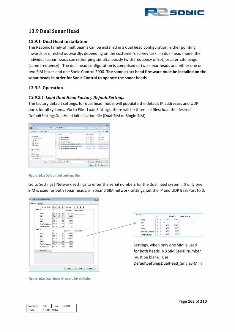
13.9 Dual Sonar Head

13.9.1 Dual Head Installation The R2Sonic family of multibeams can be installed in a dual head configuration, either pointing inwards or directed outwardly, depending on the customer’s survey task. In dual head mode, the individual sonar heads can either ping simultaneously (with frequency offset) or alternate pings (same frequency). The dual head configuration is comprised of two sonar heads and either one or two SIM boxes and one Sonic Control 2000. The same exact head firmware must be installed on the sonar heads in order for Sonic Control to operate the sonar heads.

13.9.2 Operation

13.9.2.1 Load Dual Head Factory Default Settings The factory default settings, for dual head mode, will populate the default IP addresses and UDP ports for all systems. Go to File |Load Settings, there will be three .ini files; load the desired DefaultSettingsDualHead initialisation file (Dual SIM or Single SIM).

Figure 161: Default .ini settings file

Go to Settings| Network settings to enter the serial numbers for the dual head system. If only one SIM is used for both sonar heads, in Sonar 2 SIM network settings, set the IP and UDP BasePort to 0.

Figure 162: Dual head IP and UDP defaults

Settings, when only one SIM is used for both heads. NB SIM Serial Number must be blank. Use DefaultSettingsDualHead_SingleSIM.in


13.9.2.2 Dual Head – Same Frequency – Alternating ping To operate the dual sonar heads on the same frequency it is necessary to coordinate the transmit and receive periods so there is no interference. Operating in the ‘Ping-Pong’ mode will halve the ping rate for each head, but the user gains identical acoustic resolution (such as backscatter) for both sonar heads. Please see Section 5.5.10 for head synchronisation settings.

13.9.2.3 Dual Head – Dual Frequency – Simultaneous ping Offsetting the operating frequencies, of both heads, allows the user to ping both heads simultaneously. The amount of frequency separation depends mostly on the manner in which the sonar heads have been installed and, to a lesser extent, environmental factors. Usually, the maximum separation required is 40 – 80 kHz and can be less.

Figure 163: Dual-sonar head ping modes

13.9.2.4 Dual Head with Two SIM Boxes If two SIM boxes are used, only one is the master or primary (SIM1). SIM1 will be the SIM to take in all of the serial data as well as the PPS; SIM2 only provides power to the second sonar head. SIM2 is connected to SIM1 via an Ethernet cable to one of the RJ45 ports on SIM1. In the figure, below, the bottom SIM is the primary SIM1, which takes in all of the serial data as well as timing data. The upper SIM is the secondary SIM2 that provides power to the sonar head and passes data to the primary SIM.

Figure 164: Dual Head - Dual SIM external interfacing

Secondary SIM

Primary SIM


Appendix VIII Sonic Control Commands

14 APPENDIX VIII: R2Sonic Control Commands

14.1 Introduction This describes the commands sent from the user interface to the sonar head and SIM.

Head firmware version 14-Mar-2011 and SIM firmware version 08-Apr-2010 utilize the commands in this document. Future versions of firmware will adhere to this format and may include additional commands.

Older versions of head and SIM firmware are not compatible with this format.

14.2 General Notes 1. These formats are designed for easy 4-byte alignment. Be sure your compiler/linker doesn't

insert any extra padding between values. If necessary, use your compiler's "packed" directive.

2. All values have big-endian byte order. Your compiler may provide conversion functions such as htonl, htons, ntohl, ntohs, however those assume integers so you'll need to be very careful with floats.

3. u32 means unsigned integer, 32 bits. f32 means IEEE-754 32-bit floating point.

4. All packets are UDP/IP datagrams.

5. It’s recommended that all commands be sent periodically, at a 1 to 0.5 Hz rate. This ensures that the sonar head and SIM always have the proper settings should a power interruption occur.

14.2.1 Ethernet Port Numbers Head & SIM status & command port = Baseport +2 GUI command port = 53810 (fixed port number) GUI remote command input port = gui baseport + 7

14.2.2 Type Definitions typedef unsigned int u32;

typedef float f32;

14.2.3 Command Packet Format Pseudo C format for commands: // *** BEGIN PACKET: COMMAND FORMAT 0 *** u32 PacketName; // 'CMD0' // Command (for network efficiency, the packet can contain multiple commands, // but ensure the IP datagram reaches the sonar unfragmented). u32 CommandName; // example 'RNG0' to set range x32 CommandValue; // a 4-byte value such as u32 or f32 // *** END PACKET: COMMAND FORMAT 0 ***


14.3 Head Commands, Binary Format Cmd Format Units Values Description

ABS0 f32 dB/km 0 to 200 Absorption

AIB0 f32 dB 0 to 60 Acoustic image brightness

AIH0 u32 lines 0 = off wedge radius in pixels

Acoustic imagery height. Set to display wedge radius in pixels. Head will return requested lines or less, usually less. Larger values will increase Ethernet data rate.

AUT0 u32 Flag bits 0x00000001 = auto power on 0x00000100 = auto gain on 0x00010000 = auto range on

[7:0] auto power (not functional) [15:8] auto gain (not functional) [23:16] auto range [31:24] spare Auto power/gain work in tandem, thus both are enabled/disabled at same time.

BIE0 u32 0 = off 1 = on

Bathy intensity enable

BMAX f32 metres 0 to 999 Max range filter Head default = 999 Deprecated 12 Dec 2011, see RGB0

BMIN f32 metres 0 to 500 Min range filter Head default = 0 Deprecated 12 Dec 2011, see RGA0

BOS0 u32 0 = Equiangle 1 = Equidistant

Bottom sampling

DGA0 f32 metres 0 to 1200 depth gate min

DGB0 f32 metres 0 to 1200 depth gate max

DGO0 u32 0x00000000 = gates off 0x00000001 = manual gates 0x0000ww02 = auto gates 0x0000ww03 = auto gate/slope where ww = gate width in ± percent of depth (5% to 90%)

Depth gates control. Manual gates mode require DGA0, DGB0, DGS0 to be set. In auto gates mode, a peak percentage value for gate width must be supplied in bits [15:8] in this command.

DGS0 f32 radians -π/2 to +π/2 depth gate slope

DHM0 u32 0 = single head 1 = master simultaneous, dual 2 = master alternating, dual 3 = slave simultaneous, dual 4 = slave alternating, dual

Head sync mode (single and dual head modes)

DYNA u32 0xaabbbccc aa = spare bbb = slope control ccc = depth control ex: 0x003d0523 shows a bottom at 5m depth which wobbles.

Generates a moving simulated bottom for testing auto gate features. Three control bits: [0:0] = magnitude (0-f) [1:1] = ∆ magnitude (0-f) [2:2] = rate of change (0-f) *DYNA is also supported as an ASCII command (enter hex digits without the ‘0x’)

FILT u32 0 = off 1 = range 2 = depth 3 = range & depth

FILT is deprecated. Do not use (10 Mar 2011). Use DGO0, RGA0, RGB0.

FIL0 u32 0 = single 1 = double 2 = quad

Bottom fill enhancement (High Density mode.)

FRQ0 f32 Hz 200000 to 400000, and 700000 Frequency in Hz


Cmd Format Units Values Description

GAN0 f32 1 to 45 Rcvr gain. gain in dB = setting * 2

IDCO U32 1 = Bathy+FLS proj. (model 1004) 2 = UHR proj. (model 1006)

Projector ID override, use for emergency

PNG0 u32 1 = emit one ping only Manual ping. Each time this command is sent, sonar will emit one ping.

PRL0 f32 Hz 0.1 to 60 Ping rate limit user-value

PRO0 u32 0 = projector forward 1 = projector aft

Projector orientation

PROJ u32 0 = none 1 = narrow (1°) 2 = wide (20°) (only in FLS mode)

Projector type selector

PRU0 u32 0 = off 1 = on

Ping rate limit user-enable

PRZ0 f32 metres -1.0 to +1.0 Projector mounting Z offset Default = 0.119

RET0 f32 radians -45° to +45° Receiver tilt

RGA0 f32 metres 0 to 500 Min range filter, was BMIN Head default = 0

RGB0 f32 metres 0 to 999 Min range filter, was BMAX Head default = 999

RGO0 u32 0 = range gates off 1 = range gates on

Range gate enable

RNG0 f32 metres 2 to 1200 Range

ROS0 u32 0 = off 1 = on

Roll stabilization enable

SER0 f32 radians -70° to +70° Sector rotate. Wedge edges must not go beyond ±80°

SEW0 f32 radians 10° to 160° Sector width

SNIP u32 0 = off 1 = on

Snippets enable

SPR0 f32 0 to 60 typically 20

Spreading loss

STM0 U32 0 = off 1 = on, normal mode

Status display

SVL0 f32 m/s 1250 to 1600 Sound velocity user-value

SVU0 u32 0 = use SVP 1 = user value

Sound velocity user-enable

TPG0 u32 0 = disable TruePix gates 1 = use bathy gate max 2 = use bathy gates min & max

TruePix gates

TPM0 u32 0 = off 1 = mag only 2 = mag & angle

TruePix mode.

TRG0 u32 0 = free running 1 = external trigger, SIM sync in 2 = standby, wait for PNG0 cmd.

Ping trigger source. Required, SIM command SYI0.

TWIX u32 0 = flat bottom 1 = vertical features

Bottom type

TXL0 f32 seconds 0 to 1000µs Pulse length



TXP0 f32 dB//1µPa 0, 191 to 221 Transmitter power

WCM0 u32 0 = off 1 = mag only 2 = mag & phase

Water column data. warning, high speed data, up to 70MB/s.


14.4 SIM Commands, Binary Format


BDG0 u32 bps standard baud rates 300 to 115200

GPS baud

BDH0 u32 bps standard baud rates 300 to 115200

Heading baud

BDM0 u32 bps standard baud rates 300 to 115200

Motion baud

BDS0 u32 bps standard baud rates 300 to 115200

SVP baud

DBG0 u32 7 or 8 GPS data bits

DBH0 u32 7 or 8 Heading data bits

DBM0 u32 7 or 8 Motion data bits

DBS0 u32 7 or 8 SVP data bits

DRG0 u32 0 = RS-232 1 = Ethernet

GPS driver

DRH0 u32 0 = RS232 1 = Ethernet

Heading driver (not implemented)

DRM0 u32 0 = RS-232 1 = Ethernet

Motion driver

DRS0 u32 0 = RS-232 1 = Ethernet (not implemented)

SVP driver

ENG0 u32 0 = off 1 = on

GPS serial port enable

ENH0 u32 0 = off 1 = on

Heading serial port enable Heading data not used

ENM0 u32 0 = off 1 = on

Motion serial port enable

ENS0 u32 0 = off 1 = on

SVP serial port enable

IPG0 u32 GPS IP Address

IPM0 u32 Motion sensor IP Address

PAG0 u32 0 = none 1 = odd 2 = even

GPS parity

PAH0 u32 0 = none 1 = odd 2 = even

Heading parity

PAM0 u32 0 = none 1 = odd 2 = even

Motion parity

PAS0 u32 0 = none 1 = odd 2 = even

SVP parity

POG0 u32 0 = rising 1 = falling 2 = sync on time message (no PPS)

PPS edge. Sync on time message will sync to the RS232 message; PPS pulse is not used.

PTG0 u32 0 TO 65535 GPS Ethernet port number

PTM0 u32 0 TO 65535 Motion sensor Ethernet port number.

SBG0 u32 1,2 GPS stop bits



SBH0 u32 1,2 Heading stop bits

SBM0 u32 1.2 Motion stop bits

SBS0 u32 1,2 SVP stop bits

SPO0 u32 0 = head power off 1 = head power on

Sonar head power

STM0 u32 0 = off 1 = on, normal mode

Status data

SYI0 u32 0 = off 1 = rising edge trigger 2 = falling edge trigger

Trigger in mode. Middle of transmit pulse is offset by +10ms from trigger edge. Required, Head TRG) command

SYO0 u32 0 = rises at center of tx pulse, falls at end of rcv 1 = falls at center of tx pulse, rises at end of rcv 2 = off

Trigger out mode

14.5 GUI Commands, Binary Format These commands are provided to control various GUI functions remotely. Commands are sent to GUI Baseport + 7


ABS0 f32 dB/km 0 to 200 Absorption

DGA0 f32 metres 0 to 1200 Depth gate minimum

DGB0 f32 metres 0 to 1200 Depth gate maximum

DGS0 f32 degrees -90° to +90° Depth gate slope

GAN0 f32 1 to 45 Rcvr gain. Gain in dB = setting * 2

PNG0 u32 1 = emit one ping only Manual ping. Each time this command is sent, sonar emit one ping. Sea TRG0 command

RNG0 f32 metres 2 to 1200 Range

SER0 f32 degrees -70° to +70° Sector rotate. Wedge edges must not go beyond ±80°

SEW0 f32 radians 10° to 160° Sector width

SPR0 f32 0 to 60 typically 20

Spreading loss

TXP0 f32 dB/1µPa 0, 191 to 221 Transmitter power

WCR0 u32 0 = off 1 = on

Water column enable, head 1. Equivalent to setting the water column check box in the GUI

WCR1 u32 Water column enable, head 2. Equivalent to setting the water column check box in the GUI

NB. The commands which set angle values are in degrees. This is different from angular commands sent to the head, which are in radians


14.6 Command Examples Sent to the Sonar Head and SIM Example of commands sent to the sonar head every two seconds. Columns after the command are hex, integer, and floating point representations of the data sent for each command

PacketName: CMD0

Command: ABS0 0x42a00000 1117782016 80.000000 Command: SPR0 0x41f00000 1106247680 30.000000 Command: SVL0 0x44bb8000 1153138688 1500.000000 Command: SVU0 0x00000000 0 0.000000 Command: RGO0 0x00000000 0 0.000000 Command: AUT0 0x00000000 0 0.000000 Command: RNG0 0x41a00000 1101004800 20.000000 Command: GAN0 0x41500000 1095761920 13.000000 Command: FRQ0 0x48c35000 1220759552 400000.000000 Command: TXP0 0x433f0000 1128202240 191.000000 Command: TXL0 0x37a7c5ac 933741996 0.000020 Command: SEW0 0x40060a92 1074137746 2.094395 Command: DGA0 0x40a8f312 1084814098 5.279672 Command: DGB0 0x410cca8f 1091357327 8.799453 Command: DGS0 0x00000000 0 0.000000 Command: DGO0 0x00000001 1 0.000000 Command: PRL0 0x3f800000 1065353216 1.000000 Command: PRU0 0x00000000 0 0.000000 Command: RET0 0x00000000 0 0.000000 Command: PRO0 0x00000000 0 0.000000 Command: PRZ0 0x3df3b646 1039382086 0.119000 Command: SER0 0x00000000 0 0.000000 Command: BOS0 0x00000000 0 0.000000 Command: TWIX 0x00000000 0 0.000000 Command: PROJ 0x00000001 1 0.000000 Command: ROS0 0x00000001 1 0.000000 Command: DHM0 0x00000000 0 0.000000 Command: SNIP 0x00000000 0 0.000000 Command: BIE0 0x00000000 0 0.000000 Command: AIH0 0x00000000 0 0.000000 Command: AIB0 0x40c00000 1086324736 6.000000 Command: WCM0 0x00000000 0 0.000000 Command: TPM0 0x00000000 0 0.000000 Command: TPG0 0x00000000 0 0.000000 Command: TRG0 0x00000000 0 0.000000 Command: STM0 0x00000002 2 0.000000

Example of commands sent to the SIM every two seconds. Columns after the command are hex, integer, and floating point representations of the data sent for each command

PacketName: CMD0 Command: ENG0 0x00000001 1 0.000000 Command: BDG0 0x00002580 9600 0.000000 Command: DBG0 0x00000008 8 0.000000 Command: DRG0 0x00000000 0 0.000000 Command: PAG0 0x00000000 0 0.000000 Command: SBG0 0x00000001 1 0.000000 Command: POG0 0x00000001 1 0.000000 Command: SYI0 0x00000000 0 0.000000 Command: SYO0 0x00000000 0 0.000000 Command: ENH0 0x00000001 1 0.000000 Command: BDH0 0x00002580 9600 0.000000 Command: DBH0 0x00000008 8 0.000000 Command: DRH0 0x00000000 0 0.000000 Command: PAH0 0x00000000 0 0.000000 Command: SBH0 0x00000001 1 0.000000 Command: ENM0 0x00000001 1 0.000000 Command: IPM0 0x0a00002f 167772207 0.000000 Command: POM0 0x00001388 5000 0.000000 Command: BDM0 0x00009600 38400 0.000000 Command: DBM0 0x00000008 8 0.000000 Command: DRM0 0x00000000 0 0.000000 Command: PAM0 0x00000000 0 0.000000 Command: SBM0 0x00000001 1 0.000000 Command: ENS0 0x00000001 1 0.000000 Command: BDS0 0x00002580 9600 0.000000 Command: DBS0 0x00000008 8 0.000000 Command: DRS0 0x00000000 0 0.000000 Command: PAS0 0x00000000 0 0.000000 Command: SBS0 0x00000001 1 0.000000 Command: SPO0 0x00000001 1 0.000000 Command: STM0 0x00000002 2 0.000000


Example of UDP/IP Ethernet packet of commands sent to the sonar head. First 42 characters are Ethernet header information. Characters after 29h are commands

0000 00 50 c2 90 43 3d 00 e0 81 2e be 88 08 00 45 00 .P..C=........E. 0010 01 40 7b 73 40 00 80 11 00 00 0a 00 01 66 0a 00 .@{[email protected].. 0020 00 56 06 a1 ff de 01 2c df c3 43 4d 44 30 41 42 .V.....,..CMD0AB 0030 53 30 42 a0 00 00 53 50 52 30 41 f0 00 00 53 56 S0B...SPR0A...SV 0040 4c 30 44 bb 80 00 53 56 55 30 00 00 00 00 52 47 L0D...SVU0....RG 0050 4f 30 00 00 00 00 41 55 54 30 00 00 00 00 52 4e O0....AUT0....RN 0060 47 30 41 a0 00 00 47 41 4e 30 41 50 00 00 46 52 G0A...GAN0AP..FR 0070 51 30 48 c3 50 00 54 58 50 30 43 3f 00 00 54 58 Q0H.P.TXP0C?..TX 0080 4c 30 37 a7 c5 ac 53 45 57 30 40 06 0a 92 44 47 [email protected] 0090 41 30 40 a8 f3 12 44 47 42 30 41 0c ca 8f 44 47 [email protected] 00a0 53 30 00 00 00 00 44 47 4f 30 00 00 00 01 50 52 S0....DGO0....PR 00b0 4c 30 3f 80 00 00 50 52 55 30 00 00 00 00 52 45 L0?...PRU0....RE 00c0 54 30 00 00 00 00 50 52 4f 30 00 00 00 00 50 52 T0....PRO0....PR 00d0 5a 30 3d f3 b6 46 53 45 52 30 00 00 00 00 42 4f Z0=..FSER0....BO 00e0 53 30 00 00 00 00 54 57 49 58 00 00 00 00 50 52 S0....TWIX....PR 00f0 4f 4a 00 00 00 01 52 4f 53 30 00 00 00 01 44 48 OJ....ROS0....DH 0100 4d 30 00 00 00 00 53 4e 49 50 00 00 00 00 42 49 M0....SNIP....BI 0110 45 30 00 00 00 00 41 49 48 30 00 00 00 00 41 49 E0....AIH0....AI 0120 42 30 40 c0 00 00 57 43 4d 30 00 00 00 00 54 50 [email protected] 0130 4d 30 00 00 00 00 54 50 47 30 00 00 00 00 54 52 M0....TPG0....TR 0140 47 30 00 00 00 00 53 54 4d 30 00 00 00 02 G0....STM0....

Example of UDP/IP Ethernet packet of commands sent to the SIM. First 42 characters are Ethernet header information. Characters after 29h are commands.

0000 00 50 c2 90 41 35 00 e0 81 2e be 88 08 00 45 00 .P..A5........E. 0010 01 18 7b 74 40 00 80 11 00 00 0a 00 01 66 0a 00 ..{[email protected].. 0020 00 63 06 a2 ff de 01 04 fa f0 43 4d 44 30 45 4e .c........CMD0EN 0030 47 30 00 00 00 01 42 44 47 30 00 00 25 80 44 42 G0....BDG0..%.DB 0040 47 30 00 00 00 08 44 52 47 30 00 00 00 00 50 41 G0....DRG0....PA 0050 47 30 00 00 00 00 53 42 47 30 00 00 00 01 50 4f G0....SBG0....PO 0060 47 30 00 00 00 01 53 59 49 30 00 00 00 00 53 59 G0....SYI0....SY 0070 4f 30 00 00 00 00 45 4e 48 30 00 00 00 01 42 44 O0....ENH0....BD 0080 48 30 00 00 25 80 44 42 48 30 00 00 00 08 44 52 H0..%.DBH0....DR 0090 48 30 00 00 00 00 50 41 48 30 00 00 00 00 53 42 H0....PAH0....SB 00a0 48 30 00 00 00 01 45 4e 4d 30 00 00 00 01 49 50 H0....ENM0....IP 00b0 4d 30 0a 00 00 2f 50 4f 4d 30 00 00 13 88 42 44 M0.../POM0....BD 00c0 4d 30 00 00 96 00 44 42 4d 30 00 00 00 08 44 52 M0....DBM0....DR 00d0 4d 30 00 00 00 00 50 41 4d 30 00 00 00 00 53 42 M0....PAM0....SB 00e0 4d 30 00 00 00 01 45 4e 53 30 00 00 00 01 42 44 M0....ENS0....BD 00f0 53 30 00 00 25 80 44 42 53 30 00 00 00 08 44 52 S0..%.DBS0....DR 0100 53 30 00 00 00 00 50 41 53 30 00 00 00 00 53 42 S0....PAS0....SB 0110 53 30 00 00 00 01 53 50 4f 30 00 00 00 01 53 54 S0....SPO0....ST 0120 4d 30 00 00 00 02 M0....


Appendix IX: R2Sonic Data Format

15 APPENDIX IX: R2Sonic Uplink Data Formats

15.1 Introduction This describes the data formats sent from the sonar head and SIM. Unless noted, the data packets are sent from the sonar head. The formats are given in pseudo C.

Head firmware versions 13-Dec-2011, and newer, utilise the data formats in this document. Previous head firmware versions back to 25-Mar-2010 only utilise data formats from sections 15.5 and 15.6 in this document. Future versions of firmware will adhere to this format and may include additional information.

The data format, in older versions of sonar head firmware, is different than the format described in this document and is unsupported.

15.2 General Notes 1. Each info or data section includes a name/size mini-header to allow the parser to easily skip

unneeded or unrecognized sections. These formats are designed for easy 4-byte alignment. Be sure your compiler/linker doesn't insert any extra padding between values. If necessary, use your compiler's "packed" directive.

2. All values have big-endian byte order. Your compiler may provide conversion functions such as htonl, htons, ntohl, ntohs, however those assume integers so you'll need to be very careful with floats.

3. u8, u16, u32 means unsigned integers of 8, 16, 32 bits. s8, s16, s32 means signed integers of 8, 16, 32 bits. f32 means IEEE-754 32-bit floating point.

4. All packets are UDP/IP datagrams

15.3 Port Numbers Bathymetry data port = gui.Baseport + 0 TruePix data port = tpd.Baseport + 1 Device status port = gui.Baseport + 2 Acoustic Image data port = gui.Baseport + 3 Water Column data port = wcd.Baseport + 5 Snippets data port = tpd.Baseport + 6

15.4 Type Definitions typedef unsigned char u8; typedef unsigned short u16; typedef unsigned int u32; typedef signed char s8; typedef signed short s16; typedef signed int s32; typedef float f32;


15.5 Ethernet Data Rates Bathymetry: ≈ 800 kb/s max (bathy data is sent twice, to GUI and data acquisition computer) TruePix: ≈ 5.5 Mb/s (magnitude + angle) max ≈ 3.5 Mb/s (magnitude) max Water Column: ≈ 560 Mb/s (magnitude + phase) max ≈280 Mb/s (magnitude) max Snippets: ≈ 11 Mb/s max Where Mb/s = megabits per second.


15.6 Bathymetry Packet Format // *** BEGIN PACKET: BATHY DATA FORMAT 0 ***

u32 PacketName; // 'BTH0' u32 PacketSize; // [bytes] size of this entire packet u32 DataStreamID; // reserved for future use

// section H0: header u16 H0_SectionName; // 'H0' u16 H0_SectionSize; // [bytes] size of this entire section u8 H0_ModelNumber[12]; // example "2024", unused chars are nulls u8 H0_SerialNumber[12]; // example "100017", unused chars are nulls u32 H0_TimeSeconds; // [seconds] ping time relative to 0000 hours 1-Jan-1970, integer part u32 H0_TimeNanoseconds; // [nanoseconds] ping time relative to 0000 hours 1-Jan-1970, fraction part u32 H0_PingNumber; // pings since power-up or reboot f32 H0_PingPeriod; // [seconds] time between most recent two pings f32 H0_SoundSpeed; // [meters per second] f32 H0_Frequency; // [hertz] sonar center frequency f32 H0_TxPower; // [dB re 1 uPa at 1 meter] f32 H0_TxPulseWidth; // [seconds] f32 H0_TxBeamwidthVert; // [radians] f32 H0_TxBeamwidthHoriz; // [radians] f32 H0_TxSteeringVert; // [radians] f32 H0_TxSteeringHoriz; // [radians] u32 H0_TxMiscInfo; // reserved for future use f32 H0_RxBandwidth; // [hertz] f32 H0_RxSampleRate; // [hertz] sample rate of data acquisition and signal processing f32 H0_RxRange; // [meters] sonar range setting f32 H0_RxGain; // [multiply by two for relative dB] f32 H0_RxSpreading; // [dB (times log range in meters)] f32 H0_RxAbsorption; // [dB per kilometer] f32 H0_RxMountTilt; // [radians] u32 H0_RxMiscInfo; // reserved for future use u16 H0_reserved; // reserved for future use (uncorrected pressure sensor reading in meters) u16 H0_Points; // number of bathy points


// section R0: 16-bit bathy point ranges

u16 R0_SectionName; // 'R0' u16 R0_SectionSize; // [bytes] size of this entire section f32 R0_ScalingFactor; u16 R0_Range[H0_Points]; // [seconds two-way] = R0_Range * R0_ScalingFactor u16 R0_unused[H0_Points & 1]; // ensure 32-bit section size

// section A0: bathy point angles, equally-spaced (present only during "equi-angle" spacing mode)

u16 A0_SectionName; // 'A0' u16 A0_SectionSize; // [bytes] size of this entire section f32 A0_AngleFirst; // [radians] angle of first (port side) bathy point, relative to array centerline, AngleFirst < AngleLast f32 A0_AngleLast; // [radians] angle of last (starboard side) bathy point f32 A0_MoreInfo[6]; // reserved for future use // section A2: 16-bit bathy point angles, arbitrarily-spaced (present only during "equi-distant" spacing mode) u16 A2_SectionName; // 'A2' u16 A2_SectionSize; // [bytes] size of this entire section f32 A2_AngleFirst; // [radians] angle of first (port side) bathy point, relative to array centerline, AngleFirst < AngleLast f32 A2_ScalingFactor; f32 A2_MoreInfo[6]; // reserved for future use u16 A2_AngleStep[H0_Points]; // [radians] angle[n] = A2_AngleFirst + (32-bit sum of A2_AngleStep[0] through A2_AngleStep[n]) * A2_ScalingFactor u16 A2_unused[H0_Points & 1]; // ensure 32-bit section size // section I1: 16-bit bathy intensity (present only if enabled) u16 I1_SectionName; // 'I1' u16 I1_SectionSize; // [bytes] size of this entire section f32 I1_ScalingFactor; u16 I1_Intensity[H0_Points]; // [micropascals] intensity[n] = I1_Intensity[n]) * I1_ScalingFactor u16 I1_unused[H0_Points & 1]; // ensure 32-bit section size // section G0: simple straight-line depth gates u16 G0_SectionName; // 'G0' u16 G0_SectionSize; // [bytes] size of this entire section f32 G0_DepthGateMin; // [seconds two-way] f32 G0_DepthGateMax; // [seconds two-way] f32 G0_DepthGateSlope; // [radians]


// section G1: 8-bit gate positions, arbitrary paths (present only during "verbose" gate description mode) u16 G1_SectionName; // 'G1' u16 G1_SectionSize; // [bytes] size of this entire section f32 G1_ScalingFactor; struct { u8 RangeMin; // [seconds two-way] = RangeMin * G1_ScalingFactor u8 RangeMax; // [seconds two-way] = RangeMax * G1_ScalingFactor } G1_Gate[H0_Points]; u16 G1_unused[H0_Points & 1]; // ensure 32-bit section size // section Q0: 4-bit quality flags u16 Q0_SectionName; // 'Q0' quality, 4-bit u16 Q0_SectionSize; // [bytes] size of this entire section u32 Q0_Quality[(H0_Points+7)/8]; // 8 groups of 4 flags bits (phase detect, magnitude detect, reserved, reserved), packed left-to-right // *** END PACKET: BATHY FORMAT 0 ***


15.7 Snippet Format

// *** BEGIN PACKET: SNIPPET DATA FORMAT 0 *** u32 PacketName; // 'SNI0' u32 PacketSize; // may be zero in UDP, otherwise: [bytes] size of this entire packet u32 DataStreamID; // reserved for future use // section H0: header (present only in first snippet packet of each ping) u16 H0_SectionName; // 'H0' u16 H0_SectionSize; // [bytes] size of this entire section u8 H0_ModelNumber[12]; // example "2024", unused chars are nulls u8 H0_SerialNumber[12]; // example "100017", unused chars are nulls u32 H0_TimeSeconds; // [seconds] ping time relative to 0000 hours 1-Jan-1970, integer part u32 H0_TimeNanoseconds; // [nanoseconds] ping time relative to 0000 hours 1-Jan-1970, fraction part u32 H0_PingNumber; // pings since power-up or reboot f32 H0_PingPeriod; // [seconds] time between most recent two pings f32 H0_SoundSpeed; // [meters per second] f32 H0_Frequency; // [hertz] sonar centre frequency f32 H0_TxPower; // [dB re 1 uPa at 1 meter] f32 H0_TxPulseWidth; // [seconds] f32 H0_TxBeamwidthVert; // [radians] f32 H0_TxBeamwidthHoriz; // [radians] f32 H0_TxSteeringVert; // [radians] f32 H0_TxSteeringHoriz; // [radians] u32 H0_TxMiscInfo; // reserved for future use f32 H0_RxBandwidth; // [hertz] f32 H0_RxSampleRate; // [hertz] sample rate of data acquisition and signal processing f32 H0_RxRange; // [meters] sonar range setting f32 H0_RxGain; // [multiply by two for relative dB] f32 H0_RxSpreading; // [dB (times log range in meters)] f32 H0_RxAbsorption; // [dB per kilometer] f32 H0_RxMountTilt; // [radians] u32 H0_RxMiscInfo; // reserved for future use u16 H0_reserved; // reserved for future use u16 H0_Snippets; // number of snippets f32 H0_MoreInfo[6]; // reserved for future use


// section S1: 16-bit snippet data (for network efficiency packet may contain several of these sections) (supports snippets up to 32K samples by fragmenting // at the IP level rather than by the application like 81xx) u16 S1_SectionName; // 'S1' u16 S1_SectionSize; // [bytes] size of this entire section u32 S1_PingNumber; // pings since power-up or reboot u16 S1_SnippetNumber; // snippet number, 0 to H0_Snippets-1 u16 S1_Samples; // number of samples in this snippet, sample rate is H0_RxSampleRate u32 S1_FirstSample; // first sample of this snippet relative to zero range, sample rate is H0_RxSampleRate f32 S1_Angle; // [radians] angle of this snippet, relative to array centerline f32 S1_ScalingFactorFirst; // scaling factor at start of snippet, 0=ignore, use linear interpolation to get other values f32 S1_ScalingFactorLast; // scaling factor at end of snippet, 0=ignore u32 S1_reserved; // reserved for future use u16 S1_Magnitude[S1_Samples]; // [micropascals] = S1_Magnitude[n] * (linear interpolate between S1_ScalingFactorFirst and S1_ScalingFactorLast) u16 S1_unused[S1_Samples & 1]; // ensure 32-bit section size

// *** END PACKET: SNIPPET DATA FORMAT 0 ***


15.8 Water Column (WC) Data Format // *** BEGIN PACKET: WATER COLUMN (WC) DATA FORMAT 0 *** // The water column data contains real-time beamformer 16-bit magnitude data // (beam amplitude) and optional 16-bit split-array phase data (intra-beam // direction). Maximum data rate is about 70 megabytes per second (assuming // 256 beams, 68.4 kHz sample rate, and phase data enabled). The sample rate // (and signal bandwidth) varies with transmit pulse width and range setting. // Maximum ping data size is about 32 megabytes (assuming 256 beams of 32768 // samples, and phase data enabled), but max size may change in the future. // The number of beamformed data samples normally extends somewhat further // than the user's range setting. // // When the operator enables water column mode, each sonar ping outputs // numerous 'WCD0' packets containing: one H0 header section, one A1 beam // angle section, and many M1 or M2 data sections. The section order may // change in the future, so plan for that in your data acquisition. // // Each M1 or M2 section contains a subset of the ping data. Its header // indicates its size position to help you assemble the full ping array. // // You may wish to detect missing M1 or M2 data sections (perhaps a lost // UDP packet), and then fill the gap with zeros or perhaps data from the // previous ping (to reduce visual disturbances), and then increment an // error counter for network health monitoring purposes. // // The water column data is basically in polar coordinates, so you may // wish to geometrically warp it into the familiar wedge shape for display. // Consider using OpenGL or Direct3D texture mapping. u32 PacketName; // 'WCD0' u32 PacketSize; // [bytes] size of this entire packet u32 DataStreamID; // reserved for future use // section H0: header (only one per ping) u16 H0_SectionName; // 'H0' u16 H0_SectionSize; // [bytes] size of this entire section u8 H0_ModelNumber[12]; // example "2024", unused chars are nulls u8 H0_SerialNumber[12]; // example "100017", unused chars are nulls u32 H0_TimeSeconds; // [seconds] ping time relative to 0000 hours 1-Jan-1970, integer part u32 H0_TimeNanoseconds; // [nanoseconds] ping time relative to 0000 hours 1-Jan-1970, fraction part u32 H0_PingNumber; // pings since power-up or reboot f32 H0_PingPeriod; // [seconds] time between most recent two pings f32 H0_SoundSpeed; // [meters per second]


f32 H0_Frequency; // [hertz] sonar center frequency f32 H0_TxPower; // [dB re 1 uPa at 1 meter] f32 H0_TxPulseWidth; // [seconds] f32 H0_TxBeamwidthVert; // [radians] f32 H0_TxBeamwidthHoriz; // [radians] f32 H0_TxSteeringVert; // [radians] f32 H0_TxSteeringHoriz; // [radians] u32 H0_TxMiscInfo; // reserved for future use f32 H0_RxBandwidth; // [hertz] f32 H0_RxSampleRate; // [hertz] sample rate of data acquisition and signal processing f32 H0_RxRange; // [meters] sonar range setting f32 H0_RxGain; // [multiply by two for relative dB] f32 H0_RxSpreading; // [dB (times log range in meters)] f32 H0_RxAbsorption; // [dB per kilometer] f32 H0_RxMountTilt; // [radians] u32 H0_RxMiscInfo; // reserved for future use u16 H0_reserved; // reserved for future use u16 H0_Beams; // number of beams

// section A1: float beam angles, arbitrarily-spaced (only one per ping)

u16 A1_SectionName; // 'A1' u16 A1_SectionSize; // [bytes] size of this entire section f32 A1_MoreInfo[6]; // reserved for future use f32 A1_BeamAngle[H0_Beams]; // [radians] angle of beam relative to array centerline, ordered from port to starboard, first angle < last angle // section M1: 16-bit magnitude data (present only during "magnitude-only" water column data mode, many per ping, you assemble them into complete ping data) u16 M1_SectionName; // 'M1' u16 M1_SectionSize; // [bytes] size of this entire section u32 M1_PingNumber; // pings since power-up or reboot f32 M1_ScalingFactor; // reserved for future use u32 M1_TotalSamples; // range samples in entire ping, sample rate is H0_RxSampleRate u32 M1_FirstSample; // first sample of this section u16 M1_Samples; // number of samples in this section u16 M1_TotalBeams; // beams (always a multiple of 2) (typically columns in your memory buffer) u16 M1_FirstBeam; // first beam of this section (always a multiple of 2) u16 M1_Beams; // number of beams in this section (always a multiple of 2) u32 M1_reserved0; // reserved for future use u32 M1_reserved1; // reserved for future use struct

{


u16 magnitude; // values 0 to 65535 map non-linearly (due to TVG scaling and possible gain compression) to signal amplitude } M1_Data[M1_Beams][M1_Samples]; // magnitude data (typical example: 256 beams each containing 36 two-byte structs, 16 kilobytes) // section M2: 16-bit magnitude and phase data (present only during "magnitude and phase" water column data mode, many per ping, you assemble them into // complete ping data) u16 M2_SectionName; // 'M2' u16 M2_SectionSize; // [bytes] size of this entire section u32 M2_PingNumber; // pings since power-up or reboot f32 M2_ScalingFactor; // reserved for future use u32 M2_TotalSamples; // range samples in entire ping, sample rate is H0_RxSampleRate u32 M2_FirstSample; // first sample of this section u16 M2_Samples; // number of samples in this section u16 M2_TotalBeams; // beams (always a multiple of 2) (typically columns in your memory buffer) u16 M2_FirstBeam; // first beam of this section (always a multiple of 2) u16 M2_Beams; // number of beams in this section (always a multiple of 2) u32 M2_reserved0; // reserved for future use u32 M2_reserved1; // reserved for future use struct { u16 magnitude; // values 0 to 65535 map non-linearly (due to TVG scaling and possible gain compression) to signal amplitude s16 phase; // values -32768 to +32767 map non-linearly (due to complex transfer function) to target angle within the beamwidth } M2_Data[M2_Beams][M2_Samples]; // magnitude and phase data (typical example: 256 beams each containing 36 four-byte structs, 36 kilobytes)

// *** END PACKET: WATER COLUMN (WC) DATA FORMAT 0 ***


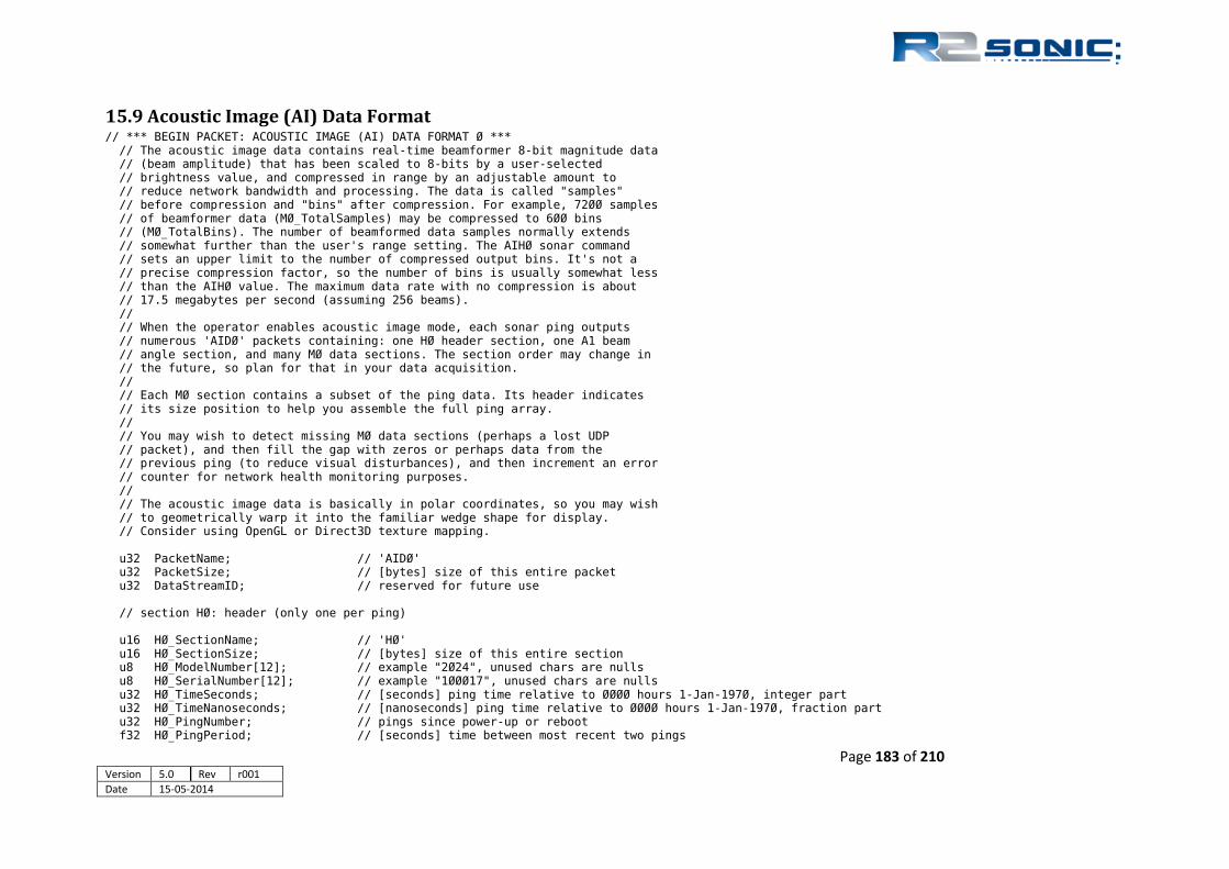
15.9 Acoustic Image (AI) Data Format // *** BEGIN PACKET: ACOUSTIC IMAGE (AI) DATA FORMAT 0 *** // The acoustic image data contains real-time beamformer 8-bit magnitude data // (beam amplitude) that has been scaled to 8-bits by a user-selected // brightness value, and compressed in range by an adjustable amount to // reduce network bandwidth and processing. The data is called "samples" // before compression and "bins" after compression. For example, 7200 samples // of beamformer data (M0_TotalSamples) may be compressed to 600 bins // (M0_TotalBins). The number of beamformed data samples normally extends // somewhat further than the user's range setting. The AIH0 sonar command // sets an upper limit to the number of compressed output bins. It's not a // precise compression factor, so the number of bins is usually somewhat less // than the AIH0 value. The maximum data rate with no compression is about // 17.5 megabytes per second (assuming 256 beams). // // When the operator enables acoustic image mode, each sonar ping outputs // numerous 'AID0' packets containing: one H0 header section, one A1 beam // angle section, and many M0 data sections. The section order may change in // the future, so plan for that in your data acquisition. // // Each M0 section contains a subset of the ping data. Its header indicates // its size position to help you assemble the full ping array. // // You may wish to detect missing M0 data sections (perhaps a lost UDP // packet), and then fill the gap with zeros or perhaps data from the // previous ping (to reduce visual disturbances), and then increment an error // counter for network health monitoring purposes. // // The acoustic image data is basically in polar coordinates, so you may wish // to geometrically warp it into the familiar wedge shape for display. // Consider using OpenGL or Direct3D texture mapping. u32 PacketName; // 'AID0' u32 PacketSize; // [bytes] size of this entire packet u32 DataStreamID; // reserved for future use // section H0: header (only one per ping) u16 H0_SectionName; // 'H0' u16 H0_SectionSize; // [bytes] size of this entire section u8 H0_ModelNumber[12]; // example "2024", unused chars are nulls u8 H0_SerialNumber[12]; // example "100017", unused chars are nulls u32 H0_TimeSeconds; // [seconds] ping time relative to 0000 hours 1-Jan-1970, integer part u32 H0_TimeNanoseconds; // [nanoseconds] ping time relative to 0000 hours 1-Jan-1970, fraction part u32 H0_PingNumber; // pings since power-up or reboot f32 H0_PingPeriod; // [seconds] time between most recent two pings


f32 H0_SoundSpeed; // [meters per second] f32 H0_Frequency; // [hertz] sonar center frequency f32 H0_TxPower; // [dB re 1 uPa at 1 meter] f32 H0_TxPulseWidth; // [seconds] f32 H0_TxBeamwidthVert; // [radians] f32 H0_TxBeamwidthHoriz; // [radians] f32 H0_TxSteeringVert; // [radians] f32 H0_TxSteeringHoriz; // [radians] u32 H0_TxMiscInfo; // reserved for future use f32 H0_RxBandwidth; // [hertz] f32 H0_RxSampleRate; // [hertz] sample rate of data acquisition and signal processing f32 H0_RxRange; // [meters] f32 H0_RxGain; // [multiply by two for relative dB] f32 H0_RxSpreading; // [dB (times log range in meters)] f32 H0_RxAbsorption; // [dB per kilometer] f32 H0_RxMountTilt; // [radians] u32 H0_RxMiscInfo; // reserved for future use u16 H0_reserved; // reserved for future use u16 H0_Beams; // number of beams // section A1: float beam angles, arbitrarily-spaced (only one per ping) u16 A1_SectionName; // 'A1' u16 A1_SectionSize; // [bytes] size of this entire section f32 A1_MoreInfo[6]; // reserved for future use f32 A1_BeamAngle[H0_Beams]; // [radians] angle of beam relative to array centerline, ordered from port to starboard, first angle < last angle // section M0: 8-bit magnitude data (many per ping, you assemble them into complete ping data) u16 M0_SectionName; // 'M0' u16 M0_SectionSize; // [bytes] size of this entire section u32 M0_PingNumber; // pings since power-up or reboot f32 M0_ScalingFactor; // reserved for future use u32 M0_TotalSamples; // range samples (before compression) in entire ping, sample rate is H0_RxSampleRate u32 M0_TotalBins; // range bins (after compression) in entire ping (M0_TotalBins <= M0_TotalSamples) u32 M0_FirstBin; // first bin of this section u16 M0_Bins; // number of bins in this section u16 M0_TotalBeams; // beams (always a multiple of 4) (typically columns in your memory buffer) u16 M0_FirstBeam; // first beam of this section (always a multiple of 4) u16 M0_Beams; // number of beams in this section (always a multiple of 4) u32 M0_reserved; // reserved for future use struct { u8 magnitude; // values 0 to 255 map non-linearly (due to TVG scaling and possible gain compression) to signal amplitude } M0_Data[M0_Beams][M0_Bins]; // magnitude data (typical example: 256 beams each containing 21 one-byte structs, 5376 bytes) // *** END PACKET: ACOUSTIC IMAGE (AI) DATA FORMAT 0 ***


15.10 TruePix™ Data Format // *** BEGIN TRUEPIX DATA FORMAT 0 *** // TruePix is like sidescan with 3D relief. Each sonar ping produces a port // and starboard time-series of data samples at the sonar's sample rate. Each // sample contains the signal's magnitude (like sidescan) and across-track // target direction angle (like bathymetry). After collecting many pings of // data along a survey line, you now have a large array of data points with // range, direction, and brightness. Apply noise reduction, and render the // data as a textured 3D surface. // // Two data formats are available: D0 provides magnitudes only, D1 provides // magnitudes and direction angles. The GUI allows the user to choose the // desired format. // // The sonar generates one TruePix data set per ping. Each data set is // usually split into multiple UDP packets. The D0 or D1 header includes // FirstSample and Samples values to help you reassemble the full data set. // // Someday you may be able to convert the 16-bit magnitude values to // micropascals by applying a to-be-determined function involving the sample // number and the MagnitudeScaling[] coefficients, but this conversion is not // yet supported so these coefficients are zero. You can convert the // direction angles from 16-bit values to radians by multiplying by // AngleScalingFactor. u32 PacketName; // 'TPX0' u32 PacketSize; // may be zero in UDP, otherwise: [bytes] size of this entire packet u32 DataStreamID; // reserved for future use // section H0: header (present only in first packet of each ping) u16 H0_SectionName; // 'H0' u16 H0_SectionSize; // [bytes] size of this entire section u8 H0_ModelNumber[12]; // example "2024", unused chars are nulls u8 H0_SerialNumber[12]; // example "100017", unused chars are nulls u32 H0_TimeSeconds; // [seconds] ping time relative to 0000 hours 1-Jan-1970, integer part u32 H0_TimeNanoseconds; // [nanoseconds] ping time relative to 0000 hours 1-Jan-1970, fraction part u32 H0_PingNumber; // pings since power-up or reboot f32 H0_PingPeriod; // [seconds] time between most recent two pings f32 H0_SoundSpeed; // [meters per second] f32 H0_Frequency; // [hertz] sonar center frequency f32 H0_TxPower; // [dB re 1 uPa at 1 meter] f32 H0_TxPulseWidth; // [seconds] f32 H0_TxBeamwidthVert; // [radians] f32 H0_TxBeamwidthHoriz; // [radians] f32 H0_TxSteeringVert; // [radians] f32 H0_TxSteeringHoriz; // [radians]


u32 H0_TxMiscInfo; // reserved for future use f32 H0_RxBandwidth; // [hertz] f32 H0_RxSampleRate; // [hertz] sample rate of data acquisition and signal processing f32 H0_RxRange; // user setting [meters] f32 H0_RxGain; // user setting [multiply by 2 for dB] f32 H0_RxSpreading; // [dB (times log range in meters)] f32 H0_RxAbsorption; // [dB per kilometer] f32 H0_RxMountTilt; // [radians] u32 H0_RxMiscInfo; // reserved for future use u32 H0_reserved; // reserved for future use f32 H0_MoreInfo[6]; // reserved for future use // section D0: 16-bit magnitude data (present only during "magnitude only" mode) u16 D0_SectionName; // 'D0' u16 D0_SectionSize; // [bytes] size of this entire section u32 D0_PingNumber; // pings since power-up or reboot u32 D0_TotalSamples; // number of samples in entire time series (sample rate is H0_RxSampleRate) u32 D0_FirstSample; // first sample of this section relative to zero range u16 D0_Samples; // number of samples in this section u16 D0_reserved; // reserved for future use f32 D0_MagnitudeScaling[8]; // to be determined, 0=ignore struct { u16 PortMagnitude; // [micropascals] = PortMagnitude * (tbd function of sample number and D0_MagnitudeScaling[8]) u16 StbdMagnitude; // similar but starboard side } D0_Data[D0_Samples]; // section D1: 16-bit magnitude and direction data (present only during "magnitude+direction" mode) u16 D1_SectionName; // 'D1' u16 D1_SectionSize; // [bytes] size of this entire section u32 D1_PingNumber; // pings since power-up or reboot u32 D1_TotalSamples; // number of samples in entire time series (sample rate is H0_RxSampleRate) u32 D1_FirstSample; // first sample of this section relative to zero range u16 D1_Samples; // number of samples in this section u16 D1_reserved; // reserved for future use f32 D1_MagnitudeScaling[8]; // to be determined, 0=ignore f32 D1_AngleScalingFactor; struct { u16 PortMagnitude; // [micropascals] = PortMagnitude * (tbd function of sample number and D1_MagnitudeScaling[8]) s16 PortAngle; // [radians from array centerline (positive towards starboard)] = PortAngle * D1_AngleScalingFactor u16 StbdMagnitude; // similar but starboard side s16 StbdAngle; // similar but starboard side } D1_Data[D1_Samples]; // *** END TRUEPIX DATA FORMAT 0 ***


15.11 Head Status Format // *** BEGIN PACKET: HEAD STATUS DATA FORMAT 0 *** // Head Status data reports the status of the sonar head. This data is // useful for troubleshooting. Data is sent to gui baseport + 2. // // Each section name consists of 4 characters. The fourth character // indicates the number of 32-bit words following each section name. // The forth character can be 1-9, A-Z; allowing up to 35 32-bit words. // The number of words in each section may change at a later date. Be // sure your program can parse the number of words. // The order of the sections is not fixed. u32 PacketName; // 'STH0' u32 PacketSize; // [bytes] size of this entire packet u32 DataStreamID; // reserved for future use // section SER3: serial number u32 SER3_SectionName; // 'SER3' u32 serial_number[3]; // example "100117", unused chars are nuls // section PRT3: part number u32 PRT3_SectionName; // 'PRT3' u32 part_number[3]; // example "15000001", unused chars are nuls // section MDL3: model number u32 MDL3_SectionName; // 'MDL3' u32 model_number[3]; // example "2024", unused chars are nuls // section FWV6: main controller firmware version u32 'FWV6'; // main ctrl firmware version string u32 version.i[6]; // example "19-Dec-2011-17:19:29", unused chars are nuls // section FWT6: internal transmitter firmware version u32 FWT6_SectionName; // 'FWT6' u32 tinytx.i[6]; // example "16-Aug-2011-17:19:29", unused chars are nuls // section PRJ9: projector

u32 PRJ9_SectionName; // ‘PRJ9’ u32 serial_number[3] // example “800456”, unused chars are nuls


u32 part_number[3]; // example “15000004”, unused chars are nuls u32 model_number[3]; // example “1004”, unused chars are nuls // section OPT1: option settings u32 OPT1_SectionName // 'OPT1' u32 options // truepix_snippets[0:0] 0=off, 1=on // depth_rating[1:1] 0=100m, 1=3km // forward_looking[2:2] 0=off, 1=on // water_column[3:3] 0=off, 1=on // ultra-high resolution[4:4] 0=off, 1=on // section SENa: sensor data received from SIM u32 SENa_SectionName; // 'SENa' u32 gps.time.sec; // [seconds]unix time u32 gps.time.nsec; // [seconds = gps.time.nsec/(2^32)] unix time f32 sensor.pitch; // [radians] mru pitch f32 sensor.roll; // [radians] mru roll f32 sensor.heave; // [meters] mru heave f32 sensor.heading; // heading (not implemented) f32 sensor.velocity; // [m/s] sound velocity f32 sensor.pdepth.uncal; // [meters] depth uncalibrated f32 sensor.pdepth.cal; // [meters] depth calibrated f32 sensor.fpgatemp; // [°C] FPGA temperature // section ADC3: a/d converter u32 ADC3_SectionName; // 'ADC3' f32 adc.chan0; // [volts] 48VDC power supply voltage f32 adc.chan1; // [amperes] 48V current f32 adc.chan8; // [volts] transmitter power supply voltage // section ETH6; ethernet registers u32 ETH6_SectionName; // 'ETH6' u32 ethernet.speed; // [megabits/sec] link connect speed u32 erxpackets; // [counts] ethernet receive packets u32 etxpackets; // [counts] ethernet transmit packets u32 erxoverflows; // [counts] ethernet receive buffer overflows u8 mac.addr[8] // mac address, use last 6 bytes, first 2 bytes are not used // section TIM2; timers u32 TIM2_SectionName // ‘TIM2’ f32 time.check; // [seconds]head to SIM roundtrip time response (must be less than 3ms) f32 time.spare; // [seconds] spare // *** END PACKET: HEAD STATUS DATA FORMAT 0 ***


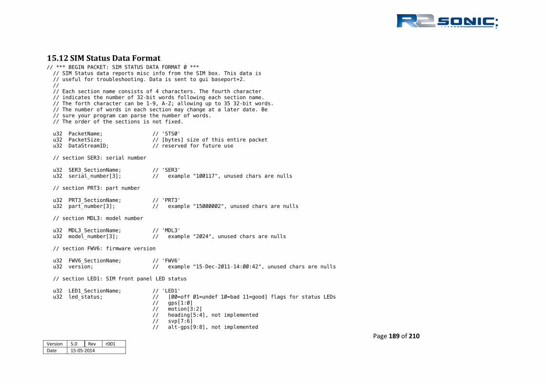
15.12 SIM Status Data Format // *** BEGIN PACKET: SIM STATUS DATA FORMAT 0 *** // SIM Status data reports misc info from the SIM box. This data is // useful for troubleshooting. Data is sent to gui baseport+2. // // Each section name consists of 4 characters. The fourth character // indicates the number of 32-bit words following each section name. // The forth character can be 1-9, A-Z; allowing up to 35 32-bit words. // The number of words in each section may change at a later date. Be // sure your program can parse the number of words. // The order of the sections is not fixed. u32 PacketName; // 'STS0' u32 PacketSize; // [bytes] size of this entire packet u32 DataStreamID; // reserved for future use // section SER3: serial number u32 SER3_SectionName; // 'SER3' u32 serial_number[3]; // example "100117", unused chars are nulls // section PRT3: part number u32 PRT3_SectionName; // 'PRT3' u32 part_number[3]; // example "15000002", unused chars are nulls // section MDL3: model number u32 MDL3_SectionName; // 'MDL3' u32 model_number[3]; // example "2024", unused chars are nulls // section FWV6: firmware version u32 FWV6_SectionName; // 'FWV6' u32 version; // example "15-Dec-2011-14:00:42", unused chars are nulls // section LED1: SIM front panel LED status u32 LED1_SectionName; // 'LED1' u32 led_status; // [00=off 01=undef 10=bad 11=good] flags for status LEDs // gps[1:0] // motion[3:2] // heading[5:4], not implemented // svp[7:6] // alt-gps[9:8], not implemented


// alt-motion[11:10], not implemented // alt-heading[13:12], not implemented // alt-svp[15:14], not implemented // pps[17:16] // sync in[19:18] // sync out[21:20] // head on[23:22] // reserved[31:24] // section SEN7: RS232 sensor values u32 SEN7_SectonName; // 'SEN7' u32 gps.time.sec; // [seconds] unix time u32 gps.time.nsec; // [seconds = gps.time.nsec/(2^32)] unix time f32 mru.pitch; // [radians] mru pitch value f32 mru.roll; // [radians] mru roll value f32 mru.heave; // [meters] mru heave f32 0.0; // heading (not implemented) f32 svp.velocity; // [m/s] sound velocity // section ADC2: a/d converter u32 ADC2_SectonName; // 'ADC2' f32 adc.chan0; // [volts] 48VDC power supply voltage f32 adc.chan1; // [amperes] 48V current to head // section ETH6: ethernet registers u32 ETH6_SectonName; // 'ETH6' u32 ethernet.speed; // [megabits/sec] link speed u32 erxpackets; // [counts] ethernet receive packets u32 etxpackets; // [counts] ethernet transmit packets u32 erxoverflows; // [counts] ethernet receive buffer overflows u8 mac.addr[8] // mac address, use last 6 bytes, first 2 bytes are not used // *** END PACKET: SIM STATUS DATA FORMAT 0 ***


15.13 Device Status Format The device status packet contains the ConfigID number that was sent to the sonar head and SIM during IP configuration. This packet contains no survey information and is ignored for data collection purposes. The R2DS packet is sent from the sonar head and SIM once per second to the sonar control program IP address. The ConfigID received from the sonar head and SIM should be compared with the ConfigID number sent to the sonar head and SIM

during IP configuration. If there is a mismatch, the control program should send IP configuration data to the sonar head and/or SIM to correct the issue.

C structure of Device Status packet

Device status Ethernet packet example received from the sonar head

Device status Ethernet packet example received from the SIM

struct R2DS // R2Sonic Device Status { u32 PacketName; // 'R2DS' u32 SerialNumber[3]; // up to 12 ASCII chars, unused chars are zero u32 ConfigID; // from most recent R2DC packet u32 spare; } pkt;

0000 00 e0 81 2e be 88 00 50 c2 90 40 58 08 00 45 00 .......P ..@ X..E. 0010 00 34 04 6c 00 00 32 11 6e 92 0a 00 00 56 0a 00 .4.l..2. n....V.. 0020 01 66 ff 16 ff de 00 20 00 00 52 32 44 53 31 30 .f..... ..R2DS10 0030 30 31 30 31 00 00 00 00 00 00 46 35 bd 01 00 00 0101.... ..;.~... 0040 00 00 ..

0000 00 e0 81 2e be 88 00 50 c2 90 40 49 08 00 45 00 .......P ..@ I..E. 0010 00 34 02 75 00 00 32 11 70 7c 0a 00 00 63 0a 00 .4.u..2. p|...c.. 0020 01 66 ff 7a ff de 00 20 00 00 52 32 44 53 31 30 .f.z... ..R2DS10 0030 30 30 34 34 00 00 00 00 00 00 46 35 bd 01 00 00 0044.... ..;.~... 0040 00 00 ..



15.14 Data Playback Using Bit-Twist

15.14.1 Introduction Note, the topics covered in this document require knowledge of Ethernet communication.

To test a data collection system, you can either use the actual hardware (sonar head) or use data captured from the sonar head. Using Wireshark, uplink data from the sonar head can be captured, filtered, and saved. Bit Twist, a console application, allows you to playback data. R2Sonic can supply sample Ethernet captures of the sonar head uplink data. You may need to edit the destination MAC and IP addresses of the captured data with Bit-Twiste, a console application. Wireshark and Bit-Twist both require Winpcap which is included in the Wireshark installation.

In the examples, the following IP addresses are used:

Sonar head: 10.0.0.86 Data collection computer: 10.0.1.102 The following programs are required: To capture, filter, and save Ethernet data: Wireshark: http://www.wireshark.org/ To playback and edit captured Ethernet data: Bit-Twist: http://bittwist.sourceforge.net/ Using a 32-bit version of Wireshark will allow you to use a packet decoder for the sonar data formats. If you don’t want or need to install Wireshark, get Winpcap at: Winpcap: http://www.winpcap.org/

15.14.2 Capturing Data To capture data from the sonar head, use Wireshark. Set the max ping rate of the sonar to 1 to 5 pings per second so you won’t create huge capture files. • Capture sonar data. For high data rate traffic, set the following Wireshark Capture Options. These options are found under the button (usually left most) “List the available capture interfaces…”. These setting will remain for the session. Buffer size: 50 megabytes Uncheck “Update list of packets in real time”


Figure 165: Wireshark Capture Options

This will reduce the processing load on Wireshark significantly. •After capture, filter the data so only the desired sonar head data is displayed. A filter expression like “not(icmp.type == 3 or ip.src == 10.0.1.102)”

can be used to filter data coming from the data acquisition computer. •Save using Save As, data type as “Wireshark/tcpdump/…- libpcap (*.pcap,*.cap)” (Wireshark default). Select “Displayed” in Packet Range. You can select a data range in the Packet Range such that the data packets aren’t truncated.

15.14.3 Editing Data The MAC and IP addresses in the packets must match the data acquisition computer’s MAC and IP addresses assigned to the network interface card (NIC). The data acquisition computer’s MAC and IP addresses can be determined using ipconfig /all from the command line. Editing the MAC and IP addresses must be done as separate operations using bittwiste.exe. The following examples show the syntax for editing the destination MAC and IP address in the .pcap files created by Wireshark. Example to change destination MAC address using bittwiste.exe: bittwiste -I in.pcap -O out.pcap -T eth -d 00:E0:12:7F:D2:1A

Example to change destination IP address using bittwiste.exe: bittwiste -I in.pcap -O out.pcap -T ip -d 10.0.1.102

Where in.pcap is the input file and out.pcap is the output file.


15.14.4 Data Playback To playback data, use bittwist.exe. You can playback data on the same computer that the data collection program resides on by simply connecting the sonar Ethernet port to an Ethernet switch. The Ethernet switch is only to placate the NIC. You can also send data from a remote computer to the data acquisition computer.

You need to determine the Ethernet interface number. Choose the interface that is connected to the sonar system. To display Ethernet interfaces:

bittwist –d

To playback data: bittwist -i 2 -l 0 out.pcap

This sends out.pcap to Ethernet interface 2 (-i 2) and loops continuously (-l 0). Use Ctrl-C to exit the program. If you don’t want to loop, use: bittwist -i 2 out.pcap



Appendix X – Drawings

16 APPENDIX X: Drawings

Drawing Index Figure 159: Sonic 2024/2022 Projector ....................................................................................................................................................................................... 198 Figure 160: Sonic 2024 Receive Module ...................................................................................................................................................................................... 199 Figure 161: Sonic 2022 Receive Module ...................................................................................................................................................................................... 200 Figure 162: Sonic 2024 Mounting Bracket Drawing 1 ................................................................................................................................................................. 201 Figure 163: Sonic 2024 Mounting Bracket Drawing 2 ................................................................................................................................................................. 202 Figure 164: Sonic 2022 Mounting Bracket Drawing 1 ................................................................................................................................................................. 203 Figure 165: Sonic 2022 Mounting Bracket Drawing 2 ................................................................................................................................................................. 204 Figure 166: Sonic 2024/2022 Mounting Bracket Flange .............................................................................................................................................................. 205 Figure 167: SIM Box Drawing ....................................................................................................................................................................................................... 206 Figure 168: SIM Stack Outline ...................................................................................................................................................................................................... 207 Figure 169: R2Sonic Deck lead minimum connector passage dimensions .................................................................................................................................. 208 Figure 170: I2NS IMU Dimensions ............................................................................................................................................................................................... 209 Figure 171: I2NS SIM Dimensions ................................................................................................................................................................................................ 210


Figure 166: Sonic 2024/2022 Projector


Figure 167: Sonic 2024 Receive Module


Figure 168: Sonic 2022 Receive Module


Figure 169: Sonic 2024 Mounting Bracket Drawing 1





Page 203 of 210

Version 5.0 Rev r001 Date 15-05-2014



Figure 173: Sonic 2024/2022 Mounting Bracket Flange


Figure 174: SIM Box Drawing


Figure 175: SIM Stack Outline


Figure 176: R2Sonic Deck lead minimum connector passage dimensions


Figure 177: I2NS IMU Dimensions


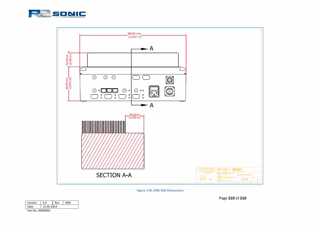
Figure 178: I2NS SIM Dimensions


Documents

Sonic 2024 Operation Manual · • June 2008 Version 1.1/1.2 • July 2008 Version 1.3 • Aug/Sep 2008 Version 1.4 • December 2008 Version 1.5 • June 2009 Version 1.6