The Psychological Record, 2012, 62, 579–598

Portions of this article will be presented at the 38th Annual Conference of the Association for Behavior Analysis International.

We gratefully acknowledge the contributions of the faculty and staff at the University of California at Irvine Machine Learning Repository for developing and sharing this scientifically collaborative website and allowing unrestricted access to so many critically important datasets.

Correspondence concerning this article should be addressed to Chris Ninness, School Psychology Program, Stephen F. Austin State University, P.O. Box 13019-SFA Station, Nacogdoches, TX 75962. E-mail: cninness@sfasu.edu

BEHAVIORAL AND PHYSIOLOGICAL NEURAL NETWORK ANALYSES: A COMMON PATHWAY TOWARD PATTERN RECOGNITION AND PREDICTION

Chris Ninness, Judy L. Lauter, Michael Coffee, Logan Clary, Elizabeth Kelly, Marilyn Rumph, Robin Rumph, and Betty Kyle

Stephen F. Austin State University

Sharon K. NinnessAngelina College

Using 3 diversified datasets, we explored the pattern-recognition ability of the Self-Organizing Map (SOM) artificial neural network as applied to diversified nonlinear data distributions in the areas of behavioral and physiological research. Experiment 1 employed a dataset obtained from the UCI Machine Learning Repository. Data for this study were composed of votes for each U.S. Representative on 16 key items during a particular legislative session. Experiment 2 employed a dataset developed in our human neuroscience laboratory and focused on the effects of sympathetic nervous system arousal on cardiac and inner-ear physiology. Experiment 3 employed the well-known Wisconsin Breast Cancer dataset, which was used to develop a sensitive, automated diagnostic method of distinguishing between malignant and benign cells. We suggest that the SOM is capable of identifying cohesive patterns of nonlinear measurements that would be difficult to identify using traditional linear data reduction procedures and that neural networks will be increasingly valuable in the analysis of a wide range of complex behaviors.Key words: Self-Organizing Map, logistic regression, pattern recognition, principal components analysis, factor analysis, prediction

While data-mining and pattern-recognition procedures are being employed at an exponential rate within basic and applied research across the natural sciences (e.g., Garbolino & Taroni, 2002; Han & Kamber, 2006; Haykin, 2009; Heaton, 2008), in many cases it may be difficult for a researcher to identify an experimental preparation as a pattern-recognition/classification problem. According to James (1985), if a botanist has a special interest in nomenclature, it is apparent that his or her primary challenge involves locating the best measurement system for classifying a sample as a member of a new or

580 NINNESS ET AL.

existing genus or species. In other types of inquiry, the strategies for employing correct classification may be less systematic. For example, our legal system is continually engaged in an attempt to identify culpability based on evidence. As James (1985) pointed out, in a particular murder case, the indicted suspect might receive a verdict indicating that he or she belongs within a classification called guilty, or the jury may deliver a verdict indicating that the individual belongs to a class of the innocent and is unreasonably accused by the state. In both circumstances, the objectives are to make the best decisions possible given the accessible evidence, and the outcomes can be thought of as forms of classification.

Within the behavioral and physiological sciences, single-subject data analysis, univariate statistics, and multivariate statistical analysis are all systems designed to help researchers make the best decisions possible given the evidence at hand (Ninness, Rumph, Vasquez, & Bradfield, 2002). Importantly, much of the evidence currently employed in an attempt to determine guilt or innocence in cases involving homicide is acquired by way of computerized pattern-recognition systems (Garbolino & Taroni, 2002). Notwithstanding, in the physiological and behavioral sciences, where an abundance of highly diversified raw information is a continually growing trend, the sheer volume of the raw data is becoming problematic. With new computer technologies disseminating a barrage of new types of measurement outcomes, researchers are often confounded by a scarcity of appropriate scientific tools for analyzing complex and previously unseen data types. The ironic but inescapable fact is that a large portion of the data we obtain in an effort to solve our scientific problems has become a major part of those problems (Gigerenzer, 2004).

Traditionally, factor analysis (FA) and principal components analysis (PCA) have been the primary multivariate tools of choice for researchers attempting to classify extremely large multifaceted datasets (Cattell, 1966; Johnson & Wichern, 2003). According to Reusch, Alley, and Hewitson (2005), PCA produces a different but simpler set of orthogonal variables that best approximates the variance in the original multifaceted and undifferentiated dataset. FA and PCA share a common mathematical foundation; however, there are differences in how these techniques are utilized in practice. Research strategies that employ FA often assume that the covariation found within diversified measurements may be a function of one or more underlying “causal” components. Usually, PCA-oriented research makes no attempt to identify underlying hypothetical constructs or attribute causation to any of the identified components; PCA is almost exclusively a data-reduction procedure designed to classify the minimal number of orthogonal components sufficient to account for most of the variance within a data structure (Child, 1990).

To obtain optimal performance from FA and PCA procedures, input values should be composed of interval or ratio data points, all of which are obtained randomly and independently (Glass, Peckham, & Sanders, 1972), precluding the possibility that the acquisition of any data point has any influence on accessing any other data point (Rummel, 1970; Stevens, 2009). While PCA and FA certainly remain essential to the analysis of particular types of problems, their fundamental underlying assumptions suggest that complementary techniques might have special value in the analysis of new types of extremely diverse and nonlinear scientific measurements (Abdi, 2003; Reyment & Jöreskog, 1993). As emphasized by Reusch et al. (2005), Self-Organizing Map (SOM) analysis differs from FA and PCA in that this procedure does not entail assumptions regarding linearity of data points, nor does it require that measurements are obtained by way of a random and independent sampling of interval or ratio scaled data points.

Early adaptations of the original SOM were used to develop pattern-recognition systems aimed at such dissimilar applications as car navigation (Pomerleau, 1991), the identification and orientation of sensitive cells in the striate cortex (Von der Malsburg, 1973), language processing with modular neural networks and distributed lexicon (Miikkulainen & Dyer, 1991), and the forecasting of earthquake aftershocks (Allamehzadeh & Mokhtari, 2003).

581NEURAL NETWORK ANALYSES

The interested reader is referred to Haykin (2009) and Duda, Hart, and Stork (2001) for detailed mathematical descriptions of these and related neural networking computational procedures. The reader can also locate SOM software developed by SAS (http://www.sas.com/technologies/analytics/datamining/miner/index.html) or SOM software by IBM SPSS (http://www-01.ibm.com/software/analytics/spss/products/statistics/neural-networks/). Alternatively, the reader may contact the first author for sample input data and a downloadable SOM application (Ninness, 2012) developed at the SFA Behavioral Software Design Laboratory, installable on Windows operating systems (see Appendix).

Even though SOM algorithms fall under the heading of unsupervised neural networks developed for the purpose of identifying concealed data patterns within chaotic or nonlinear distributions, finding a common input metric (scaling system) has been a continuing challenge in the general application of these algorithms. This is particularly true when the input data are composed of extremely diversified measurement metrics (e.g., blood pressure, intelligence, or body weight). Here, the output patterns showing common trends among different data types have been inconsistent or less impressive (e.g., Arciniegas-Rueda, Daniel, & Embrecths, 2001). In fact, to date, there is no generally accepted transformation strategy for scaling heterogeneous data types.

To address this issue, we have been working to make the SOM capable of converting raw scores to z scores, and the version we describe here is capable of analyzing diverse inputs in accordance with a user’s preference. If a given dataset is composed of different metrics, the most straightforward strategy is to transform all data to z scores and run the SOM analysis using z scores rather than raw scores. If the raw data is composed of binary values (e.g., voting for or against), raw scores can be converted to dummy/indicator variables.

As described previously, new computer technologies are inundating researchers with diversified and chaotic measurement outcomes (Kline, 2009). Thus, one of the studies in this article focuses on physiological data. These data are included to demonstrate the conceptual integrity and broad applicability of SOM neural network applications. In two of the studies presented, we attempted to make predictions based on logistic regression procedures.

The central restriction regarding multiple linear regression entails the assumption regarding a continuous dependent variable. Many interesting variables in the analysis of behavior and physiology are dichotomous or categorical. For example, public school students may attend or not attend classes, legislators may vote yea, nay, or present. A cell may be benign or malignant. A variety of regression techniques have been developed for analyzing data with different types of dependent variables, including multiple linear regression, discriminant analysis, and logistic regression. Logistic regression is traditionally employed when there are discrete classifications of the dependent variable.

Similar to multiple linear regression procedures, logistic regression calculates formulas for any dependent variable of interest and a series of b coefficients that indicate each independent variable’s weighted influence on the dependent variable under consideration. For a given categorical variable, an equation is created that includes all weighted predictor variables that are valuable in making this prediction. Two of the studies in this article move past pattern recognition into a logistic regression analysis in an attempt to develop prediction strategies.

Taken together, these three studies are intended as demonstrations of neural network pattern recognition capability when aimed at extremely dissimilar and nonlinear dependent variables. Such variables are not unlike those obtained in many current findings in behavior analysis (e.g., Ninness et al., 2005). We (Ninness et al., 2005) used an earlier version of this architecture in conjunction with our computer-interactive mathematic software to identify and remediate mathematical errors that occurred during computer-based instruction. In the current study, we attempt to expand our previous neural network procedures.

582 NINNESS ET AL.

General MethodUsing three challenging, nonlinear, and multifaceted datasets, we explored the

pattern-recognition ability of the SOM neural network as adapted by Ninness and colleagues and applied it to datasets composed of qualitatively different scales. Experiment 1 employed a dataset obtained from the UCI Machine Learning Repository (Frank & Asuncion, 2010) and was composed of votes for each of the U.S. Representatives on 16 key items during a particular legislative session. Experiment 2 examined within-subject changes in a group of nine human physiological variables measured before, during, and after use of a cold pressor challenge. Experiment 3 was conducted with the well-known Wisconsin Breast Cancer dataset donated to the UCI Machine Learning Repository. These data were used to develop a sensitive, automated diagnostic method to distinguish between malignant and benign cells. As described on the UCI Machine Learning Repository homepage, the repository is composed of a collection of complex databases, domain theories, and data generators that are used by the statistical and machine learning community for the empirical analysis of machine learning algorithms (Frank & Asuncion, 2010). Given our research ambition to demonstrate the SOM neural network’s ability to identify and systematically organize irregular and extremely diverse measurements, these three datasets met our criteria for multidimensionality. Our immediate ambition for this study was to test our version of the SOM using these three dissimilar datasets in an effort to obtain output patterns that would be difficult to isolate and classify using traditional statistical procedures. Our long-term ambition was and is to further develop our version of the SOM such that it will not only identify nonlinear data patterns but will concurrently predict future behavioral and physiological outcomes using a logistic regression procedure in conjunction with our SOM neural network software. As per Hopkins, Hopkins, and Glass (1996), “the purpose of a regression equation is to make predictions for a new, but comparable, sample for which the scores on the independent variable are available” (p. 125). To employ logistic analysis with precision, sample size should be above 300 (Stevens, 1996). The dataset from Experiment 2 was too small to allow prediction procedures; however, in Experiment 1, we used our version of the SOM in conjunction with logistic regression to predict the likelihood of particular votes being cast by members of the U.S. House of Representatives.

Using data from Experiment 3, we used the SOM in conjunction with a logistic regression procedure to predict the likelihood of particular cells being malignant or benign. While a multiple linear regression procedure can be employed when the outcome of interest can be measured on a linear interval or ratio scale, multiple logistic regression is the procedure of choice when the dependent variable is categorical or dichotomous. Logistic regression examines the weighted influence of independent variables by computing the probability of occurrence regarding a specific event. Logistic regression does not assume a linear association between the dependent and the aggregate of independent variables (Johnson & Wichern, 2003).

Experiment 1According to details provided by Schlimmer (1987) and downloaded from the UCI

Machine Learning Repository, this dataset entails 16 key votes made by members of the U.S. House of Representatives. These congressional votes were simplified to their basic tally format consisting of Yea, Nay, or Present.

MethodTo change the raw data to a numerical format, Nay votes were converted to values of

1, votes for representatives who were simply unavailable or votes cast as Present (to avoid conflict) were transformed to 1.5, and Yea votes were transformed to values of 2. The

583NEURAL NETWORK ANALYSES

congressional votes then took on numeric values that were equidistant and meaningful in the sense that the nonoccurrence of a vote, which may have been a function of a member’s attempt to avoid conflict or a member’s inability to be on location at a given point in time, had the effect of “splitting the weighted difference” between an affirmative and negative contribution to the group decision.

ResultsAfter converting votes to numerical dummy scores and conducting SOM-based

analysis, four distinct patterns emerged, as shown in Figure 1. Class 1 is a voting pattern representing 31.03% of all and 88.88% of the Republican House membership across all 16 key legislative items. Class 2 is a pattern representing 24.03% of all and 85.8% of the Democratic votes. Class 3 is an SOM pattern representing 34.71% of all and 94.66% of the Democratic members of the House. With 9.88% of its total, Class 4 is poorly differentiated because it includes a combination of Republican and Democratic House members who exhibited inconsistent voting patterns.

Class 1 Class 2

Class 3 Class 4

94.66% Democratic (34.71% of all)

88.88% Republican (31.03% of all)

67.44% Democratic (9.88% of all)

85.8% Democratic (24.03% of all) 1 2 3 4 5 6 7 8 9 10 11 12 13 14 15 16

350

300

250

200

150

100

50

0 1 2 3 4 5 6 7 8 9 10 11 12 13 14 15 16

350

300

250

200

150

100

50

0

1 2 3 4 5 6 7 8 9 10 11 12 13 14 15 16

350

300

250

200

150

100

50

0 1 2 3 4 5 6 7 8 9 10 11 12 13 14 15 16

350

300

250

200

150

100

50

0

Figure 1. SOM classifications of voting patterns. Four voting patterns emerged from the SOM analysis of 435 Members of the U.S. House of Representatives on 16 key bills during the 98th Congress.

Given a member’s voting record on this particular series of 16 key legislative items, it is possible to identify the individual’s party affiliation with a high level of accuracy.

584 NINNESS ET AL.

Although members of both parties abstained on any given bill, and any member may have voted in favor or in opposition to a particular item, the three dominant voting patterns are identified by the SOM neural network. Data within Class 4 (approximately 10% of all) were ambiguous, and these data were extracted prior to developing prediction formulas (see Kuyuk, Yildirim, Dogan & Horasan, 2011, for a similar SOM filtering strategy employed by seismologists).

Employing the 392 well-classified data patterns within Classes 1, 2, and 3, a follow-up logistic regression identified the probability of particular members being affiliated with one party or the other. In Figure 2, the first 249 markers refer to Democratic members, while the remaining 143 votes were cast by Republican members. Based on three voting patterns classified by the SOM, we identified party affiliation for 98.2% (385/392) of legislators within these three neural-network-defined classes as described in the logistic regression procedures that were computed on psyNet Software (Ninness, 2012) and matched SPSS calculations (where p = .0000) as follows:z = − 26.032 + 0.4723x1 − 0.978x2 − 5.157x3 + 14.029x4 + 4.458x5 − 5.154x6 + 8.219x7 − 1.166x8 − 2.133x9 + 3.866x10 − 3.296x11 + 0.259x12 − 0.903x13 + 2.537x14 − 1.345x15 + 1.379x16

1 + e− z

1Prob = (1)

Democratic and Republican House Members

1 14 27 40 53 66 79 92 105

118

131

144

157

170

183

196

209

222

235

248

261

274

287

300

313

326

339

352

365

378

391

Prob

ablili

ty th

at a

ser

ies

of 1

6 ke

y vo

tes

were

cas

t by

a Re

publ

ican

1

0.9

0.8

0.7

0.6

0.5

0.4

0.3

0.2

0.1

0

Figure 2. Logistic regression identified the probability of 392 House member party affiliations based on voting patterns identified by the SOM. The first 249 votes were cast by Democratic House members, and the remaining 143 were cast by Republican House members.

Figure 3 shows the series of actual votes for each House member as a heavy dark line where a Nay vote is located along line 1, the nonoccurrence of a vote, or a vote of Present, falls at 1.5, and Yea votes are shown along line 2. The probability of each of the 392 legislators voting for Key Bill Number 4 (Adoption of the Budget Resolution) using the logistic regression formula (where p = .0000) is the following: Based on three voting patterns classified by the SOM, we predicted the voting patterns for 97.44% (382/392) of legislators within these three neural-network-defined classes, as described in the logistic regression formula:z = −16.5393 − 0.956x1 + 1.694x2 + 0.253x3 + 1.533x4 + 0.004x5 − 1.421x6 + 0.095x7 + 1.110x8 − 0.558x9 + 0.374x10 + 1.232x11 + 1.353x12 + 0.206x13 + 0.406x14 − 1.930x15 + 8.394x16

585NEURAL NETWORK ANALYSES

Clearly, we could not have used SOM unless we already knew the information that we sought to predict in the regression equation. The first 233 votes were recorded as Nay, followed by 6 Present votes located at 1.5, and the remaining 153 indicated votes recorded as Yea. Markers showing the voting predictions for each House member are based on the classification of voting patterns within parties as identified by the SOM and subsequently predicted by logistic regression.

Prob

ablili

ty o

f Vot

ing

Yea

on B

ill Nu

mbe

r 4

Democratic and Republican House Members

1 13 25 37 49 61 73 85 97 109

121

133

145

157

169

181

193

205

217

229

241

253

265

277

289

301

313

325

337

349

361

373

385

1

0.9

0.8

0.7

0.6

0.5

0.4

0.3

0.2

0.1

0

Figure 3. Logistic regression–based probability of 392 House members voting Nay, Present, or Yea on Key Bill Number 4. The first 233 votes (located at 0) show actual votes recorded as Nay, the next 6 (located at 0.5) indicate a vote of Present, and the remaining 153 (located at 1) are votes recorded as Yea.

Experiment 2The second experiment employed a single-subject design to determine the existence of

coordinated effects of sympathetic nervous system activation on certain physiological aspects of the heart and the inner ear. The study was employed using the cold pressor test (placing one hand up to the wrist in ice water for a brief period), which is an established means of noninvasively activating the sympathetic nervous system (cf. Robertson, 2004), along with a variety of dependent variables related to cardiac and inner-ear function. Tests were conducted in the Human Neuroscience Laboratory at Stephen F. Austin State University, following guidelines from the Auditory Cross-Section Test Battery (AXS; Lauter, 2000), and employing an A-B-A design during which the participant was exposed to four prepressor blocks, followed by three blocks of pressor challenges, and ending with four postpressor blocks.

MethodDuring each of the series of 11 test blocks (approximately 1 min each), the subject sat

quietly in a comfortable chair while a Marshall blood pressure cuff was used to collect three dependent variables representing cardiac function: diastolic blood pressure, systolic blood pressure, and heart rate. At the same time, during each of the blocks, an Otodynamics computer system was used to collect five dependent variables of inner-ear physiology, as reflected in different aspects of transient evoked otoacoustic emissions (TEOAEs; cf. Dhar & Hall, 2009): two measures of the overall response amplitude (coded as response and X [mean] response), a variability measure comparing overall response amplitude in

586 NINNESS ET AL.

back-to-back single-click trials (coded A-B), and the amplitude of response analyzed in frequency bands centered around 1 kHz, 2 kHz, and 3 kHz. The dataset for this subject (3 cardiac variables and 5 ear variables for each of 11 test blocks) was transformed to z scores and analyzed for pattern recognition by the SOM neural network. One graduate student served as the participant in this experiment. A preliminary SOM analysis was conducted to see how the output would appear in the absence of transformation of z scores.

Results and DiscussionOutcomes derived from raw data showed extremely wide dispersion among the

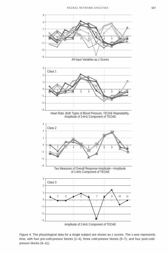
variables in the construction of the SOM feature map. In the absence of SOM-based analyses, outcomes did not demonstrate any form of recognizable data patterns or any clear differentiation among variables. After converting all data to z scores and entering the data into the SOM network, several classifications were identified, while one category (response amplitude at 2 kHz) was unique. In order to show the cohesive flow of data, A-B-A phase lines are not displayed before and after the cold pressor test condition; however, Figure 4 shows that the two classes containing more than one function grouped the following variables: (a) Class 1: all three cardiac measures, together with two TEOAE measures (A-B and 3 kHz response amplitude) and (b) Class 2: three TEOAE measures (response, X response, 1 kHz response amplitude). Class 3, amplitude of 2 kHz of TEOAE, is a unique but well-differentiated dependent variable.

Class 1: First, all three cardiac measures showed increases during cold pressor, which is consistent with previous findings (cf. Robertson, 2004), which demonstrates that this challenge is an effective activator of the sympathetic nervous system. Second, the SOM associated the TEOAE variability function (A-B) with the three cardiac measures, suggesting that increases in blood pressure may be causally related to increases in run-to-run variability in cochlear responsivity. Such a finding is consistent with the well-established dependence of the highly vascularized cochlea on the biophysics of its blood supply (Dallos, 1996). Thus, in this case, perturbations in blood pressure associated with sympathetic arousal may be reflected in TEOAE variability. Third, the increase in response amplitude at 3 kHz during cold pressor may be related to the tonotopic nature of the basilar membrane within the cochlea. That is, parts of the basilar membrane closer to the basal end of the cochlea (which is more narrow and thicker than areas tuned to lower frequencies) may be more sensitive to blood pressure changes.

Class 2: The association of three of the TEOAE measures (response, mean response, and response amplitude at 1 kHz), and the fact that they all involved a decrease in response amplitude, may reflect the action of a central physiological process recruited to reduce the response to peripheral pain (in this case, when one hand is placed in ice water). The observation of decreased amplitudes in at least some TEOAE measures suggests that this central sensory-reduction process has global effects and is not limited to the pain-related somatosensory system. Finally, as indicated above, Class 3: amplitude of the 2-kHz TEOAE, is a unique but well-differentiated dependent variable.

Experiment 3The third study focused on the identification of breast cancer cells computed by way

of digitized images of cell nuclei. The original Wisconsin Breast Cancer dataset was donated to the UCI Machine Learning Repository. Wolberg (1992) provided the samples from his clinical cases from the University of Wisconsin Hospitals (Wolberg, Street, Heisey, & Mangasarian, 1995). These data have been used in statistical analyses and neural network research to develop a sensitive, automated diagnostic method to distinguish between malignant and benign cells that would be less intrusive than surgical biopsy (e.g., You & Rumbe, 2010). As described by Wolberg et al. (1995), variable attributes in the database were computed from the digital images of the fine needle aspirates (FNA) of breast masses to describe the characteristics of the cell nuclei in the images among

587NEURAL NETWORK ANALYSES

All Input Variables as z Scores

Heart Rate, Both Types of Blood Pressure, TEOAE Repeatablity, Amplitude of 3-kHz Component of TEOAE

Class 1

Class 2

Class 3

Two Measures of Overall Response Amplitude + Amplitude of 1-kHz Component of TEOAE

Amplitude of 2-kHz Component of TEOAE

3

2

1

0

−1

−2

−3

3

2

1

0

−1

−2

−3

3

2

1

0

−1

−2

−3

3

2

1

0

−1

−2

−3

1 2 3 4 5 6 7 8 9 10 11

1 2 3 4 5 6 7 8 9 10 11

1 2 3 4 5 6 7 8 9 10 11

1 2 3 4 5 6 7 8 9 10 11

Figure 4. The physiological data for a single subject are shown as z scores. The x-axis represents time, with four pre-cold-pressor blocks (1–4), three cold-pressor blocks (5–7), and four post-cold-pressor blocks (8–11).

588 NINNESS ET AL.

569 participants. The cytological characteristics of breast FNA variables included 10 primary variables calculated for each cell nucleus. Specifically, these included the, “radius (mean of distances from center to points on the perimeter), texture (standard deviation of gray-scale values), perimeter, area, smoothness (local variation in radius lengths), compactness, concavity (severity of concave portions of the contour), concave points (number of concave portions of the contour), symmetry, fractal dimension (of the boundary)” (Demyanov, Bagirov, & Rubinov, 2002, p. 77).

MethodPrior to transformation to z scores, we attempted to run a SOM analysis. Outcomes

derived from raw data showed extremely wide dispersion among the variables in the construction of the SOM feature map. In the absence of transformation to z scores, outcomes did not demonstrate any form of recognizable data patterns or any clear differentiation between benign and malignant cells. When the 569 data points were converted to z scores and reanalyzed by the SOM neural network, several well-differentiated patterns emerged.

Results and DiscussionSOM outcomes revealed that 70.31% of the cases were classified in accordance with

cells being benign or malignant. Figure 5 illustrates SOM classifications. Since we had access to the follow-up outcomes based on surgical biopsy, we were able to verify the accuracy of all predictions. Specifically, Class 1 (12.5% of all data) was composed of 100% benign cells. Class 2 (32.51% of all data) was composed of 96.7% benign cells, and Class 3 (25.3% of all data) was composed of 99.3% malignant cells (cf. Demyanov et al., 2002). As shown in Figure 5, class differentiation appeared to be based on five key variables: worst radius, mean texture, standard error of the local variation in radius lengths, standard error of concave points, and mean of the three largest concave points. Arrows within Class 3 in Figure 5 point to these variable locations, which contrast with the same locations within Class 1 and Class 2 of this figure. Class 4 was composed of an almost even distribution of benign and malignant cells; thus, data within this class were excluded from post-hoc analysis. Figure 6 illustrates the risk of malignancy based on a logistic regression employing the 406 cases that fell within Classes 1, 2, and 3. Logistic regression procedures were computed on psyNet Software (Ninness, 2012) and SPSS. Both statistical packages produced the following multiple regression formula:z = 487.248 − 59.057x1 − 57.599x2 − 2.549x3 + 2.966x4 − 70.406x5

(2)1 + e−z

1Risk =

In Figure 6, a false positive prediction falls above 0.5 on the y-axis (and a false negative falls below 0.5 on the y-axis). Following SOM analysis, logistic regression generated an overall 99.51% level of accuracy with only two false positive and no false negative predictions. The above outcomes compare favorably with other machine learning studies predicting breast cancer based on FNA findings (Dutra et al., 2011).

To be clear, logistic regression was employed to confirm that the SOM had succeeded in clustering cases in a manner which allowed us to exclude cases that were statistically noisy. We could not have used SOM unless we already knew the information that we sought to predict in the regression equation. Notwithstanding, classification of a new or existing case might be conducted in two parts. Given a previously unexamined case obtained by FNA containing 30 real-valued input features, these variables could be entered into the existing database, preprocessed to z scores, and analyzed for classification by the SOM neural network. If the case fell into a pattern consistent with any of the three

589NEURAL NETWORK ANALYSES

Figure 5. The Wisconsin Breast Cancer dataset following transformation data of all 569 cases to z scores.

100% Benign (12.5% of Total) 96.7% Benign (32.51% of Total)

99.3% Malignant (25.3% of Total) Undifferentiated (29.7% of Total)

1 3 5 7 9 11 13 15 17 19 21 23 25 27 29

6

5

4

3

2

1

0

−11 3 5 7 9 11 13 15 17 19 21 23 25 27 29

6

5

4

3

2

1

0

−1

1 3 5 7 9 11 13 15 17 19 21 23 25 27 29

6

5

4

3

2

1

0

−11 3 5 7 9 11 13 15 17 19 21 23 25 27 29

6

5

4

3

2

1

0

−1

Class 1 Class 2

Class 3 Class 4

Figure 6. Risk of malignancy based on SOM neural network analysis and logistic regression.

Prob

ablili

ty o

f Mal

igna

ncy

1 13 25 37 49 61 73 85 97 109

121

133

145

157

169

181

193

205

217

229

241

253

265

277

289

301

313

325

337

349

361

373

385

397

1

0.9

0.8

0.7

0.6

0.5

0.4

0.3

0.2

0.1

0

590 NINNESS ET AL.

well-differentiated groups (and this would be expected to occur approximately 70.31% of the time), the data could be further analyzed by way of logistic regression.

Summary and Concluding DiscussionIn Experiment 1, Republican and Democratic Congressional votes originally tallied

and recorded in the forms of Y, ?, or N were converted to a numerical scale as indicator/dummy variables (Draper & Smith, 1998; Roscoe, 1975). Using this indicator scale, we transformed Nay votes to numerical values of 1, votes from representatives who were simply unavailable or votes cast as Present (to avoid conflict) were transformed to 1.5, and Yea votes were transformed to values of 2.

The voting records classified as undifferentiated (9.88%) were extracted from the origi-nal dataset, and a follow-up logistic regression was conducted. As a result, party affiliations, as well as the probability of particular legislators voting for or against a key piece of legisla-tion were predicted accurately. In Experiment 2 we examined within-subject changes in a group of nine physiological variables observed before, during, and after exposure to a cold pressor challenge, and clearly defined classifications emerged across conditions. In Experiment 3 we addressed cell diagnostics. SOM outcomes revealed that 70.31% of the cases were classified in accordance with cells being benign or malignant. Class 1 was com-posed of 100% benign cells. Class 2 was composed of 96.7% benign cells, and Class 3 was composed of 99.3% malignant cells. Subsequently, multiple logistic regressions produced an overall 99.51% level of accuracy (cf. Paulin & Santhakumaran, 2009).

The SOM is capable of isolating/classifying data clusters with cohesive topological features that are critical to solving a very wide range of problems. During SOM analysis, a particular class may emerge as unified and well differentiated from other classes; however, the class may be functionally irrelevant to a particular problem at hand. For example, Kuyuk et al. (2011) employed a SOM in their classification of earthquakes and found approximately 6% of classifications contained unified topological features. These data were equivocal and extracted (filtered) from their prediction model. Kuyuk et al. describe this model as extremely robust and sufficiently reliable for laboratory practice in the forecasting of seismic events.

In Experiment 1 of this study, 9.88% of the Congressional voting data were extracted from the original dataset prior to making accurate predictions. In Experiment 3, 29.7% of the Wisconsin Breast Cancer dataset formed a nonlinear classification of cells, but this particular class did not differentiate between benign and malignant cells. Thus, these data were extracted prior to generating predictions by way of logistic regression. In these experiments, the a priori extraction of topologically similar but functionally irrelevant classes allowed logistic regression to be employed with greater precision (see Rousseeuw & Leroy, 2001, for a discussion of robust regression procedures). Removing unreliable or irrelevant classes/clusters could be construed as a less than desirable approach to making important predictions regarding future events; however, in many studies there may be considerable strategic advantage in systematically filtering unreliable or irrelevant classes within a dataset. One can make extremely broad spectrum but less precise and less reliable predictions based on employing all available data, or one can extract a class known to be composed of irrelevant outcomes and proceed toward making more accurate but qualified predictions based on SOM pattern recognition (cf. Allamehzadeh & Mokhtari, 2003).

While many classification/pattern recognition studies may not lend themselves to logis-tic regression, other types of research may be informed by these techniques. For example, given a sufficiently large database, predicting subtle physiological changes that accompany exposure to cold pressor (Experiment 2) might lead to several important neuroscience predic-tions. While acknowledging that our research in the area of predicting voting behavior, and the likelihood of cells being benign or malignant is in the preliminary stages of development, it appears that further investigation in this area is warranted. Given the predictions in the article, forecasting party affiliations (Experiment 1), as well as the probability of particular

591NEURAL NETWORK ANALYSES

legislators voting for or against key pieces of legislation, could be a subject of some value and interest. Likewise, the accurate prediction of cells as benign or malignant (Experiment 3) may well have implications for future investigations (Abbass, 2002). In total, these findings may contribute to future behavioral/physiological investigations.

We should point out that the SOM neural network classification thresholds are “adjustable.” That is, although the fundamental algorithm is a constant, the SOM’s classification threshold can be set to various levels of sensitivity in order to identify increasingly inconspicuous pattern formations within a nonlinear dataset. This is true for all neural networks (Behnke, 2003; Heaton, 2008); interestingly, it is consistent with the way in which factor analysis operates. For example, orthogonal rotations sustain the original perpendicular relations among all components on the coordinate axes, whereas oblique rotations do not require that factors sustain their orthogonal relations (Abdi, 2003; Rummel, 1970; Stevens, 2009). While FA and PCA remain essential to the analysis of a wide range of problems, their fundamental underlying assumptions suggest that complementary techniques might have special value in the analysis of new types of extremely diverse and nonlinear scientific measurements (Reusch et al., 2005).

As a prospect for ongoing research and related software development, we continue to expand our development of neural network functionality in conjunction with traditional data reduction procedures such as principal components analysis. Our ambition is to generate better functionality, user interactivity, and develop our software’s ability to accurately recognize and predict a wider range of critically important outcomes within the behavioral and physiological sciences. The extent to which we are able to demonstrate increasing levels of precision remains an empirical question.

ReferencesABBASS, H. A. (2002). An evolutionary artificial neural networks approach for breast

cancer diagnosis. Artificial Intelligence in Medicine, 25, 265–281.ABDI, H. (2003). Factor rotations. In M. Lewis-Beck, A. Bryman, & T. Futing (Eds.),

Encyclopedia for research methods for the social sciences (pp. 978–982). Thousand Oaks, CA: Sage.

ALLAMEHZADEH, M., & MOKHTARI, M. (2003). Prediction of aftershocks distribution using Self-Organizing Feature Maps (SOFM) and its application on the Birjand-Ghaen and Izmit earthquakes. Journal of Seismology and Earthquake Engineering, 5, 1–15.

ARCINIEGAS-RUEDA, I., DANIEL, B., & EMBRECTHS, M. (2001). Exploring financial crises data with self-organizing maps (SOM). In N. Allinson, L. Allinson, H. Yin, & J. Slack (Eds.), Advances in Self-Organizing Maps (pp. 30–39). London, England: Springer-Verlag.

BEHNKE, S. (2003). Hierarchical neural networks for image interpretation( LNCS/LNAI). Berlin, Germany: Springer-Verlag.

CATTELL, R. B. (1966). The scree test for the number of factors. Multivariate Behavioral Research, 1, 245–276.

CHILD, D. (1990). The essentials of factor analysis (2nd ed). London: Cassel Educational Limited.

DALLOS, P. (1996). The cochlea. New York, NY: Springer-Verlag.DEMYANOV, V. F., BAGIROV, A. M., & RUBINOV, A. M. (2002). A method of truncated

codifferential with application to some problems of cluster analysis. Journal of Global Optimization, 23, 63–80.

DHAR, S., & HALL, J. W. III. (2009). Otoacoustic emissions: Principles, procedures, protocols. San Diego, CA: Plural.

DRAPER, N. R., & SMITH, H. (1998). Applied regression analysis. New York, NY: Wiley.

592 NINNESS ET AL.

DUDA, R., HART, P., & STORK, D. (2001). Pattern classification (2nd ed.). New York, NY: Wiley.

DUTRA, I., NASSIF, H., PAGE, D., SHAVLIK, J., STRIGEL, R., WU, Y., . . . BURNSIDE, E. (2011). Integrating machine learning and physician knowledge to improve the accuracy of breast biopsy. Proceedings of the American Medical Informatics Association Symposium (AMIA’11), Washington, DC: 349–355.

FRANK, A., & ASUNCION, A. (2010). UCI Machine Learning Repository [http://archive.ics.uci.edu/ml]. Irvine, CA: University of California, School of Information and Computer Science.

GARBOLINO, P., & TARONI, F. (2002). Evaluation of scientific evidence using Bayesian networks. Forensic Science International, 125, 129–155.

GIGERENZER, G. (2004). Mindless statistics. Journal of Socio-Economics, 33, 587–606.GLASS, G. V., PECKHAM, P. D., & SANDERS, J. R. (1972). Consequences of failure to meet

assumptions underlying the fixed-effects analysis of variance and covariance. Review of Educational Research, 42, 237–288.

HAN, J., & KAMBER, M. (2006). Data mining: Concepts and techniques (2nd ed.). San Francisco, CA: Morgan Kaufmann.

HAYKIN, S. S. (2009). Neural networks and learning machines (3rd ed.). Upper Saddle River, NJ: Prentice Hall.

HEATON, J. (2008). Introduction to neural networks for C# (2nd ed.). St. Louis, MO: Heaton Research, Inc.

HOPKINS, K. D., HOPKINS, B. R., & GLASS, G. V. (1996). Basic statistics for the behavioralsciences (3rd ed.). Needham Heights, MA: Allyn & Bacon.

JAMES, M. (1985). Classification algorithms. Hoboken, NJ: Wiley.JOHNSON, R. A., & WICHERN, D. W. (2003). Applied multivariate statistical analysis

(5th ed.). Upper Saddle River, NJ: Prentice Hall.KLINE, R. B. (2009). Becoming a behavioral science researcher: A guide to producing

research that matters. New York, NY: Guilford Press.KUYUK, H. S., YILDIRIM, E., DOGAN, E., & HORASAN, G. (2011). An unsupervised learning

algorithm: Application to the discrimination of seismic events and quarry blasts in the vicinity of Istanbul. Natural Hazards and Earth System Sciences, 11, 93–100.

LAUTER, J. L. (2000). The AXS battery and neurological fingerprints: Meeting the challenge of individual differences in human brain/behavior relations. Behavioral Research Methods, Instruments, and Computers, 32, 180–190.

MIIKKULAINEN, R., & DYER, M. G. (1991). Natural language processing with modular PDP networks and distributed lexicon. Cognitive Science, 15, 343–399.

NINNESS, C. (2012). psyNet SOM (Version 1) [Behavioral Software Design Systems]. Nacogdoches, TX: Stephen F. Austin State University. Retrieved from http://www.faculty.sfasu.edu/ninnessherbe/chris_ninness.htm

NINNESS, C., RUMPH, R., MCCULLER, G., HARRISON, C., VASQUEZ, E., FORD, A., . . . BRADFIELD, A. (2005). A relational frame and artificial neural network approach to computer-interactive mathematics. The Psychological Record, 55, 561–570.

NINNESS, C., RUMPH, R., VASQUEZ, E., & BRADFIELD, A. (2002). Multivariate randomization tests for small-n behavioral research. Behavior and Social Issues, 12, 64–74.

PAULIN, F., & SANTHAKUMARAN, A. (2009). Extracting rules from feed forward neural networks for diagnosing breast cancer. International Journal of Artificial Intelligent Systems and Machine Learning, 1(4), 143–146.

593NEURAL NETWORK ANALYSES

POMERLEAU, D. (1991). Efficient training of artificial neural networks for autonomous navigation. Neural Computation, 3, 88–97.

REUSCH, D. B., ALLEY, R. B., & HEWITSON, B. C. (2005). Relative performance of self-organizing maps and principal component analysis in pattern extraction from synthetic climatological data. Polar Geography, 29, 227–251.

REYMENT, R. A., & JÖRESKOG, K. G. (1993). Applied factor analysis in the natural sciences. Cambridge, England: Cambridge University Press.

ROBERTSON, D. (2004). Primer on the autonomic nervous system (2nd ed.). San Diego, CA: Elsevier Academic Press.

ROSCOE, J. T. (1975). Fundamental research statistics for the behavioral sciences (2nd ed.). New York, NY: Holt, Rinehart & Winston.

ROUSSEEUW, P. J., & LEROY, A. (2001). Robust regression and outlier detection. New York, NY: Wiley.

RUMMEL, R. J. (1970). Applied factor analysis. Evanston, IL: Northwestern University Press.SCHLIMMER, J. C. (1987). 1984 United States Congressional voting records database

[UCI Machine Learning Repository]. Irvine, CA: University of California, School of Information and Computer Science. Retrieved from http://archive.ics.uci.edu/ml/

STEVENS, J. P. (1996). Applied multivariate statistics for the social sciences (3rd ed.). Mahwah, NJ: Erlbaum.

STEVENS, J. P. (2009). Applied multivariate statistics for the social sciences (5th ed.). Hillsdale, NJ: Erlbaum.

VON DER MALSBURG, C. (1973). Self-organization of orientation sensitive cells in the striate cortex. Kybernetik, 14, 85–100.

WOLBERG, W. (1992). Breast cancer Wisconsin (diagnostic) dataset [UCI Machine Learning Repository]. Irvine, CA: University of California, School of Information and Computer Science. Retrieved from http://archive.ics.uci.edu/ml/

WOLBERG, W., STREET, W., HEISEY, D., & MANGASARIAN, O. (1995). Computer-derived nuclear features distinguish malignant from benign breast cytology. Human Pathology, 26, 792–796.

YOU, H., & RUMBE, G. (2010). Comparative study of classification techniques on breast cancer FNA biopsy data. International Journal of Artificial Intelligence and Interactive Multimedia, 3, 5–12.

594 NINNESS ET AL.

AppendixThe interested user can download our version of the Self-Organizing Map

(http://www.faculty.sfasu.edu/ninnessherbe/chris_ninness.htm) by clicking on the SOM_2012.zip link located near the top of our webpage. After downloading the zipped file (which includes the SOM and a sample dataset) to your desktop, right click the folder, “extract all,” and deploy. Only the cyan-colored buttons are relevant to this study. The screen shot below is an illustration from Microsoft Office 2010. Other versions of Office may appear slightly different; however, the operations described below will be exactly the same. Please contact the first author (cninness@sfasu.edu) if instillation or other complications should occur.

1. Make sure your dataset is saved as a CSV file.

2. Open the psyNet application on your desktop and click Kohonen SOM z-Attributes. 3. For the sample data provided, enter 4 into the textbox labeled Cols, and 150 into the textbox labeled Rows.

4. Click Kohonen SOM z-Attributes. At this point, a window will open and you will be able to select your dataset, which must already be saved in CSV format (see Step 1).

5. Double click the icon containing your CSV dataset.

595NEURAL NETWORK ANALYSES

6. At this point, you will be able to see the SOM output data within the psyNet listbox on the left side of the application.

7. Click on Save Outcome CSV File. Another window will open. Type in a new file name. Give this CSV extension a name that you can easily locate. Usually, it is helpful to save this new file to your desktop. Again, make sure the file is saved in the CSV format.

8. Close the psyNet application and open your new CSV file.

9. You will see an Excel Spreadsheet in CSV format with numbers in columns. The sequence of data points are identified in Column A in the same order in which these data were entered into the program. Column B identifies the class names generated by the SOM for each vector in this particular dataset. These classes (identified by numbers) are arbitrary and change each time the SOM application is employed.

596 NINNESS ET AL.

10. Highlight all columns and rows except those with “0” so that all data in these columns are shaded/grayed out.

11. Once highlighted, click Data on the tab at the top of your Excel toolbar, then click Sort. A window will open. Click Sort by and select Column B. Then, click OK.

12. Your data is now sorted by numerical class name. Column B represents the specific classifications within this dataset. From here you can begin creating graphs for each classification identified by the SOM.

13. Position your cursor in the first row of Column B containing data. Highlight all data until the category changes, including the associated columns. (For example, your highlighted range might be B1…F50.)

597NEURAL NETWORK ANALYSES

-2

-1.5

-1

-0.5

0

0.5

1

1.5

2

1 2 3 4

1 2 3 4

-2

-1.5

-1

-0.5

0

0.5

1

1.5

2

1 2 3 4

-2

-1.5

-1

-0.5

0

0.5

1

1.5

2

1 2 3 4

-2

-1.5

-1

-0.5

0

0.5

1

1.5

2

Iris Setosa in z score units following SOM analysis

Undifferentiated class composed of three members

represented in z scores following SOM analysis

Iris Versicolor in z scores units following SOM analysis

Iris Virginica in z scores units following SOM analysis

14. Once your data is properly highlighted, click Insert at the top of the screen, under Review select Line, and choose a 2-D line graph.

15. Click Switch Rows/Columns.

16. Repeat the previous steps for each remaining category (Column B).

If you were to run the Iris dataset a second time (with LL at 3), the class names would change; however, the composition of each of the SOM classes will remain exactly the same.

598