Embed Size (px)
Citation preview
Sommerfeld corrections in
neutralino dark matter pair-annihilations
and relic abundance in the general MSSM
Dissertation
vorgelegt von
Charlotte Hellmann
Betreuer: Prof. Dr. Martin Beneke
Lehrstuhl fur Theoretische Elementarteilchenphysik T31
Fakultat fur Physik
der Technischen Universitat Munchen

TECHNISCHE UNIVERSITAT MUNCHEN
Lehrstuhl fur Theoretische Elementarteilchenphysik T31
Sommerfeld corrections in neutralino dark matter
pair-annihilations and relic abundance in the general MSSM
Anna Charlotte Hellmann
Vollstandiger Abdruck der von der Fakultat fur Physik
der Technischen Universitat Munchen zur Erlangung des akademischen Grades eines
Doktors der Naturwissenschaften
genehmigten Dissertation.
Vorsitzender: Univ.-Prof. Dr. Lothar Oberauer
Prufer der Dissertation: 1. Univ.-Prof. Dr. Martin Beneke
2. Univ.-Prof. Dr. Alejandro Ibarra
3. Univ.-Prof. Dr. Michael Klasen,
Westfalische Wilhelms-Universitat Munster
(nur schriftliche Beurteilung)
Die Dissertation wurde am 03.12.2014 bei der Technischen Universitat Munchen
eingereicht und durch die Fakultat fur Physik
am 13.02.2015 angenommen.

Abstract
It is intriguing that the observed dark matter abundance in our Universe can be explainedrather naturally as thermal relic of a weakly interacting massive particle. Probablythe most popular such particle dark matter candidate is the lightest neutralino in theMinimal Supersymmetric Standard Model (MSSM). In this thesis we study the impactof Sommerfeld enhancements on the neutralino relic abundance calculation for heavyneutralino dark matter in the general MSSM including co-annihilations of further nearlymass-degenerate neutralino and chargino states. To this end we develop an effective fieldtheory that systematically resums the enhanced radiative corrections to pair-annihilationrates of slowly moving neutralinos and charginos. The framework is applied to heavywino- and higgsino-like scenarios and models interpolating between these cases.
iii

iv
Zusammenfassung
Die in unserem Universum beobachtete Dunkelmaterie kann in naturlicher Weise als ther-misches Relikt eines schwach wechselwirkenden massiven Teilchens erklart werden. Einsolcher vielversprechender Dunkelmaterie-Teilchenkandidat ist das leichteste Neutralinoim Minimalen Supersymmetrischen Standardmodell (MSSM). In der vorliegenden Arbeitwird der Einfluss der Sommerfeld-Verstarkung auf die Neutralino Reliktdichte fur schwereNeutralino Dunkelmaterie-Kandidaten im allgemeinen MSSM und unter Einbeziehungvon Co-Annihilationseffekten weiterer naherungsweise massenentarteter Neutralino- undChargino-Spezies untersucht. Dazu wird eine effektive Theorie entwickelt, die uberhohteStrahlungskorrekturen in Paar-Annihilationen langsamer Neutralinos und Charginos re-summiert. Der Formalismus wird auf Wino- und Higgsino-artige Szenarien angewandt,sowie auf Modelle, die zwischen diesen Fallen extrapolieren.
v

vi
Contents
1 Introduction 5
2 Sommerfeld enhancements in a toy scenario 13
2.1 The origin of the enhancement . . . . . . . . . . . . . . . . . . . . . . . . 142.2 An enhancement formula for a N -state model . . . . . . . . . . . . . . . 18
2.3 N = 1 state models with Coulomb and Yukawa potential interactions . . 31
2.3.1 One-state model with Coulomb potential . . . . . . . . . . . . . . 33
2.3.2 One-state model with Yukawa potential . . . . . . . . . . . . . . . 35
2.4 A two-state model with off-diagonal interactions . . . . . . . . . . . . . . 39
3 Relic abundance calculation 47
3.1 The Boltzmann equation . . . . . . . . . . . . . . . . . . . . . . . . . . . 47
3.2 Co-annihilations . . . . . . . . . . . . . . . . . . . . . . . . . . . . . . . . 523.3 Thermally averaged annihilation cross sections . . . . . . . . . . . . . . . 56
4 The neutralino and chargino sector in the MSSM 594.1 Motivations for supersymmetry and basic ideas . . . . . . . . . . . . . . 59
4.2 The MSSM: field content and parameters . . . . . . . . . . . . . . . . . . 62
4.3 The neutralino and chargino sector . . . . . . . . . . . . . . . . . . . . . 65
4.4 MSSM spectrum generation . . . . . . . . . . . . . . . . . . . . . . . . . 69
5 Effective theory description of neutralino pair annihilations 71
5.1 The Lagrangian in the effective theory . . . . . . . . . . . . . . . . . . . 71
5.2 χ0/χ± pair-annihilations in the NRMSSM . . . . . . . . . . . . . . . . . 755.2.1 Basis of dimension-6 operators in δLann . . . . . . . . . . . . . . . 77
5.2.2 Basis of dimension-8 operators in δLann . . . . . . . . . . . . . . . 80
6 The hard annihilation reactions 836.1 Matching calculation & Master formula . . . . . . . . . . . . . . . . . . . 84
6.1.1 Matching condition . . . . . . . . . . . . . . . . . . . . . . . . . . 84
6.1.2 Expansion in momenta and mass differences in δLann . . . . . . . 86
6.1.3 Unitary vs Feynman gauge . . . . . . . . . . . . . . . . . . . . . . 90
6.1.4 A master formula for the Wilson coefficients . . . . . . . . . . . . 91
1

6.2 Numerical comparison:Tree-level annihilation rates . . . . . . . . . . . . . . . . . . . . . . . . . 956.2.1 χ+
1 χ+1 →W+W+ and χ+
1 χ−1 →W+W− . . . . . . . . . . . . . . . 99
6.2.2 The S-wave dominated processes χ01χ
+1 → tb, ud . . . . . . . . . . 100
6.2.3 The P -wave dominated reaction χ+2 χ
−2 → h0h0 . . . . . . . . . . . 102
6.2.4 The off-diagonal χ+1 χ
−1 →W+W− → χ+
2 χ−2 rate . . . . . . . . . . 104
6.2.5 Annihilation cross sections of “hydrogen-like” χχ states . . . . . . 1066.3 Application of the analytic results at O(v2
rel):
A pure-wino NRMSSM sample calculation . . . . . . . . . . . . . . . . . 1076.3.1 Coupling factors . . . . . . . . . . . . . . . . . . . . . . . . . . . 1086.3.2 Kinematic factors . . . . . . . . . . . . . . . . . . . . . . . . . . . 1116.3.3 Exclusive pure-wino NRMSSM co-annihilation rates . . . . . . . . 114
7 Long-range potential interactions 1197.1 NRMSSM potentials: Matching calculation . . . . . . . . . . . . . . . . . 1197.2 Matrix representation of NRMSSM potentials . . . . . . . . . . . . . . . 126
7.2.1 The two possibles bases of χχ states in the NRMSSM . . . . . . . 1277.2.2 Pure-wino NRMSSM potential & annihilation matrices . . . . . . 130
8 Sommerfeld enhancement 1338.1 Sommerfeld-corrected annihilation rates . . . . . . . . . . . . . . . . . . . 1348.2 NR matrix-elements & the Schrodinger equation . . . . . . . . . . . . . . 1398.3 Sommerfeld factors in the method-1 and 2 bases . . . . . . . . . . . . . . 1468.4 Solution of the Schrodinger equation: improved method . . . . . . . . . . 1478.5 Second-derivative operators . . . . . . . . . . . . . . . . . . . . . . . . . 1548.6 Approximate treatment of heavy channels . . . . . . . . . . . . . . . . . 156
9 Benchmark models in the general MSSM 1639.1 Wino-like χ0
1 . . . . . . . . . . . . . . . . . . . . . . . . . . . . . . . . . . 1649.2 Higgsino-like χ0
1 . . . . . . . . . . . . . . . . . . . . . . . . . . . . . . . . 1729.3 Light scenario . . . . . . . . . . . . . . . . . . . . . . . . . . . . . . . . . 1799.4 Higgsino-to-wino trajectory . . . . . . . . . . . . . . . . . . . . . . . . . 1829.5 Mixed wino-higgsino χ0
1 . . . . . . . . . . . . . . . . . . . . . . . . . . . . 190
10 Conclusions 197
A Absorptive parts of Wilson coefficients of dimension-6 and 8operators in δLann 201A.1 Coupling factors . . . . . . . . . . . . . . . . . . . . . . . . . . . . . . . . 202
A.1.1 Coupling factor construction . . . . . . . . . . . . . . . . . . . . . 202A.1.2 (Axial-)vector and (pseudo-)scalar MSSM vertex factors . . . . . 205
A.1.3 Example: construction of c(α)n,i1V
in χ−e1χ
+e2 →W+G− → χ0
e4χ0e3 . . . 209
A.2 Kinematic factors at leading order . . . . . . . . . . . . . . . . . . . . . . 210A.2.1 Kinematic factors for XAXB = V V . . . . . . . . . . . . . . . . . 212
2
A.2.2 Kinematic factors for XAXB = V S . . . . . . . . . . . . . . . . . 214A.2.3 Kinematic factors for XAXB = SS . . . . . . . . . . . . . . . . . 216A.2.4 Kinematic factors for XAXB = ff . . . . . . . . . . . . . . . . . . 217A.2.5 Kinematic factors for XAXB = ηη . . . . . . . . . . . . . . . . . . 220
A.3 Kinematic factors at O(v2) . . . . . . . . . . . . . . . . . . . . . . . . . . 221A.3.1 P -wave kinematic factors for XAXB = V V . . . . . . . . . . . . . 222A.3.2 P -wave kinematic factors for XAXB = V S . . . . . . . . . . . . . 226A.3.3 P -wave kinematic factors for XAXB = SS . . . . . . . . . . . . . 230A.3.4 P -wave kinematic factors for XAXB = ff . . . . . . . . . . . . . 233A.3.5 P -wave kinematic factors for XAXB = ηη . . . . . . . . . . . . . . 236
B Explicit expressions for the MSSM potentials in Lpot 239
C Equivalence between method-1 and method-2 241
3

4
Chapter 1
Introduction
The existence of a cold dark matter (DM) component in our Universe is by now wellestablished by various observations and at all experimentally accessible scales, rangingfrom the size of galaxies to galaxy clusters and large scale structures up to the largestobservable scales associated with the cosmic microwave background radiation (CMB) [1].For instance, the fact that galactic rotation curves become approximately constant anddo not decrease with increasing distance from the galactic centre is explained by thepresence of halos of non-luminous and non-absorbing – hence dark – matter. Similarobservations and explanations in terms of dark matter exist for galaxy clusters. Themost accurate determination of the present cold dark matter density Ωcdmh
2 is relatedto cosmological precision measurements and has reached percent level accuracy: from acombination of PLANCK, WMAP, baryon acoustic oscillation (BAO) and high resolutionCMB data, a value of
Ωcdmh2 = 0.1187± 0.0017 (1.1)
is obtained [2], where h denotes the Hubble constant in units of 100 km /(sMpc).In spite of evidence for its existence, the nature and origin of the cold dark mat-
ter component are still unknown. The Standard Model (SM) of particle physics thathas been tested extensively by experiments and that describes so far successfully themicroscopic interactions of the constituents associated with ordinary matter (quarks,gluons, leptons, neutrinos, the photon, the electroweak gauge bosons and the SM Higgsboson) [1],provides no particle dark matter candidate. This in turn is one of the fewempirical evidences that the SM cannot be the fundamental theory of nature. Assumingthat dark matter has particle nature, possible extensions of the SM should therefore in-volve a particle dark matter candidate that is stable or at least sufficiently long lived oncosmic timescales. Furthermore this particle candidate may not interact with photonsnor take part in strong interactions, otherwise dark matter would be visible or it wouldhave been found in rare isotopes [3, 4].
It is intriguing that the origin of the observed cosmic cold dark matter abundancecan be explained rather naturally through thermal production and subsequent freeze-out of a particle with weak interaction strength and a TeV scale mass, a so called
5
weakly interacting massive particle (WIMP) [3,4]. This might indicate that new physicsat the TeV scale, which is needed to addresses certain formal issues in the SM suchas the stability of the electroweak scale, is also associated with a cosmic dark matterconstituent, thereby connecting problems related to the smallest and largest observablescales. The explanation of the cosmic cold dark matter abundance in terms of a coldrelic implies that the corresponding freeze-out process in the early Universe takes place attemperatures when the DM particles become non-relativistic. An accurate determinationof the relic density considers also the presence and freeze-out of those further species inthe early Universe, that are close-in-mass and interact with the DM candidate. Thecentral ingredients in the relic abundance calculation are the pair-annihilation rates ofthe DM and additional nearly mass-degenerate particles. Given that the DM particleshave typical non-relativistic velocities v ∼ 0.2 c around freeze-out, the correspondingtree-level co-annihilation cross sections can be expanded according to
σannvrel = a + b v2rel + O(v4rel) , (1.2)
where vrel = |~v1 − ~v2| is the relative velocity of the two annihilating particles in theircentre-of-mass frame. Referring to tree-level rates and keeping only the first two termsin the expansion is often a good approximation in the relic abundance calculation.
In the simple freeze-out scenario DM pair-annihilation reactions eventually ceasewhen the DM number density is sufficiently diluted due to the expansion of the Universe.However, pair-annihilation reactions can restart when DM eventually accumulates in thepresent Universe due to gravitational interactions. Corresponding regions with a DMover-density can be galactic centres, but also the sun potentially has a sufficient gravita-tional potential to attract, capture and amass DM particles. The DM pair-annihilationreactions occurring today in these regions are described by the same annihilation rates(1.2) as in the early Universe. Since the typical velocities of the annihilating particlestoday are however much smaller, v ∼ 10−3 c, it is often enough to consider the leadingorder term a in the non-relativistic expansion of the corresponding annihilation crosssections.
Certainly one of the most studied and probably best motivated DM candidates isthe lightest neutralino (χ0
1) in the Minimal Supersymmetric Standard Model (MSSM)[3, 4], a sypersymmetric extension of the SM. There exist several codes that allow forthe calculation of the χ0
1 relic density in the general MSSM, currently relying on tree-level annihilation rates and taking co-annihilation reactions with further supersymmetricparticles close in mass with the χ0
1 into account [5, 6]. The calculated relic density of aviable χ0
1 dark matter candidate should at least not exceed the observed Ωcdmh2 value.
The latter allows for the possibility that the cosmic dark matter is constituted by severalparticle species, each contributing a certain portion to the total dark matter abundance.From the requirement that the χ0
1 explains all observed cosmic dark matter in terms of athermal χ0
1 relic, stringent constraints on the MSSM parameter space can be derived [7,8].The actual identification of a particle dark matter candidate with the cosmic con-
stituent relies on the complementarity of different experimental search strategies; forcorresponding investigations related to the χ0
1 DM candidate see for instance the recent
6
publications [9,10]. The aforementioned pair-annihilation reactions in the galactic centreor the sun would produce indirect signals of dark matter particles, revealing themselvesin cosmic or gamma ray signatures or neutrino fluxes, looked for with correspondingspace or ground-based telescopes. Direct detection experiments are searching for signalsfrom scattering reactions of DM particles off terrestrial detector materials. To assign(future) signals from indirect and direct detection experiments to a certain candidate,this particle should ideally be produced directly at a particle collider such as the LargeHadron Collider (LHC) at CERN, which would allow to determine – or at least narrowdown – some of its properties as for instance its mass and spin. Let us mention herethat in the past several experimental collaborations working on direct and indirect DMdetection have reported the observation of signals, which they claimed could not be ex-plained by known backgrounds or other astrophysical sources and which therefore couldbe assigned to dark matter. However the explanation as dark matter signals in noneof these cases is definitely confirmed and former DM indications could later often beattributed to underestimated background or detector effects.
In this thesis we focus on the neutralino relic abundance calculation and improveits accuracy by systematically resuming a certain class of radiative corrections to therelevant neutralino and chargino co-annihilation cross sections. Indeed, given the experi-mental percent level accuracy on Ωcdmh
2, (1.1), it seems desirable to include radiativecorrections to the co-annihilation rates, which enter the relic abundance calculationas a central ingredient and are currently afflicted with the largest uncertainties. Twodifferent approaches in refining the determination of the co-annihilation rates of the χ0
1
and further close-in-mass MSSM states can be distinguished. On the one hand, next-to-leading order corrections to the co-annihilation rates are calculated in fixed orderperturbation theory in the general MSSM. The determination of the complete next-to-leading order SUSY QCD corrections in neutralino and chargino pair-annihilations,including co-annihilations with possibly nearly mass-degenerate sfermion states has beenfinalised recently [11–15]. Moreover, the first steps in the calculation of the full next-to-leading order electroweak corrections have been carried out [16–18]. On the otherhand there exists a class of radiative corrections that can be enhanced in non-relativisticneutralino co-annihilation reactions and eventually requires systematic resummation upto all orders in perturbation theory. This situation generically arises in theories that allowfor light mediator exchange between heavy non-relativistic DM particles prior to theirannihilation. The light mediator exchanges give rise to long-range potential interactionsthat distort the incoming DM particles’ wave-functions away from plane waves, suchthat their annihilation probability becomes larger. In terms of Feynman diagrams, theeffect is associated with amplitudes that exhibit ladder-like exchanges of the mediatorsbetween the co-annihilating non-relativistic DM particles before the latter actually pair-annihilate. Each loop in the corresponding diagrams involves a contribution that scalesas g2mDM/mφ, where g denotes the respective coupling, mφ the mediator mass and mDM
refers to the DM mass scale. For sufficiently light mediator masses, mφ ≪ mDM, theseterms are unsuppressed and eventually lead, after systematic resummation, to the so-called Sommerfeld enhancement of the corresponding annihilation rate. In the MSSM
7

with χ01 dark matter candidate the mutual exchange of electroweak gauge bosons, and to a
lesser extend light Higgs bosons, causes the Sommerfeld enhancement in heavy neutralinopair-annihilations. Sommerfeld enhancements are associated with the non-relativisticnature of the pair-annihilating particles. They are typically the stronger the smaller thevelocities of the particles. Consequently the relevance of the Sommerfeld enhancementeffect for χ0
1 DM has first been pointed out in context of gamma ray signatures from χ01
pair-annihilations in the galactic centre today [19,20], where the authors considered thesimplified scenarios of pure wino and pure higgsino χ0
1 states. Although the enhancementeffect is much milder during χ0
1 freeze-out because of the larger mean velocities (v ∼ 0.2 c)it was found in [20] that its impact on the relic density can be significant for purewino χ0
1 DM. Subsequently, the Sommerfeld enhancement effect in the MSSM has beenstudied extensively both in application to indirect detection and the χ0
1 relic abundancecalculation [21–27], where these analyses mainly referred to the limiting scenarios of wino-or higgsino-like χ0
1 or even pure wino and pure higgsino χ01 models. In addition, in [28]
Sommerfeld enhancements were investigated in context of “minimal dark matter” modelsthat resemble the MSSM in the limits of pure wino and pure higgsino DM. In additionto MSSM related studies, there have been several investigations on the Sommerfeldenhancement effect in generic dark matter models. In particular, the measurement ofan anomalous positron excess by the PAMELA experiment in 2008 has triggered severalinvestigations on Sommerfeld enhancements in generic dark matter models, where theeffect was considered as a means to boost the DM annihilation rates in the presentUniverse while at the same time providing electroweak scale cross sections during freeze-out due to much milder enhancement factors at larger velocities [29].
In this thesis we address Sommerfeld enhancement effects in co-annihilation reactionsof nearly mass-degenerate neutralinos and charginos in the general MSSM, extendingprevious work on the subject in several important aspects. With the term “generalMSSM” we imply that our calculations allow an application to any generic R-parityconserving MSSM scenario. In particular, the χ0
1 can be an arbitrary admixture ofthe electroweak gaugino and higgsino gauge-eigenstates, away from the strict wino andhiggsino limits. Further important improvements or extensions to existing investigationsin the literature are the following:
• We use an effective theory framework to describe the pair-annihilation reactions ofnon-relativistic and nearly mass-degenerate neutralino and chargino pairs, similarto the NRQCD approach to heavy quarkonium annihilations in [30]. An impor-tant difference to the latter QCD case is the fact that we deal with several nearlymass-degenerate scattering states χeaχeb . The exchange of electroweak gauge orlight Higgs bosons prior to the short-distance annihilation allows for potentialscattering transitions from an initially incoming pair χiχj to another such nearlymass-degenerate two-particle state. In the effective theory we therefore encounterdiagonal as well as off-diagonal potential interactions. These are of Coulomb-typefor photon exchange (which corresponds to a purely diagonal potential scatter-ing reaction) but are Yukawa-like in case of electroweak gauge boson and Higgsexchange. We determine analytic expressions for all (off-) diagonal potential inter-
8

actions at leading-order in the non-relativistic expansion.
• The effective field theory approach by construction provides a factorisation be-tween the long-range and short-distance contributions to the co-annihilation rates.The total pair-annihilation cross section of an incoming χiχj pair is related tothe absorptive part of the forward scattering amplitude χiχj → . . . → χe1χe2 →∑XAXB → χe4χe3 → . . . χiχj , where XAXB denotes a pair of SM or light Higgs
particles. Due to the presence of off-diagonal potential interactions χeaχeb →χecχed, changing the nature of the incoming two-particle state prior to annihilation,the short-distance annihilations encoded in reactions χe1χe2 →
∑XAXB → χe4χe3
are generically associated with off-diagonal processes as well, where the χe1χe2 pairis not necessarily identical to the χe4χe3 pair. Off-diagonal annihilation rates wereonly known in the pure wino and higgsino limits and at leading order in the non-relativistic expansion. They have not been considered previously in applicationsto the generic MSSM. We derive purely analytical results for all (off-) diagonalshort-distance annihilation rates. In the effective theory they are encoded in theabsorptive parts of Wilson coefficients and are automatically partial-wave sepa-rated. We determine not only the leading order S-wave contributions, but alsocalculate P -wave and next-to-next-to-leading order S-wave terms associated withthe term b in (1.2).
• The determination of the Sommerfeld enhancement factors for an incoming χiχjstate in a certain partial-wave configuration requires the solution of a matrixSchrodinger equation involving matrix-valued potentials that refer to correspond-ing (off-) diagonal potential scattering reactions. As we allow the neutralino andchargino states in the effective theory to exhibit small mass differences, there willbe potential transitions to kinematically closed two-particle channels. If the masssplittings between the incoming and the closed channels become larger, numericalinstabilities arise in the solution of the Schrodinger equation. We discuss a novelmethod based on an appropriate reformulation of the Schrodinger problem thatsolves this issue.
• The Sommerfeld factors depend on the partial wave state of the annihilating pair.Consequently, the consistent determination of the Sommerfeld-enhanced annihi-lation rates requires a partial wave separation of the short-distance annihilationrates. In particular the P - and next-to-next-to-leading order S-wave contributionsto the coefficient b in (1.2) have to be known separately. Within the effective theorywe obtain such partial wave separation by construction.
A number of limitation of our framework has to be mentioned. The formalism in its cur-rent form does not allow to cover resonant s-channel annihilations in the short-distancerates, as the process is no longer short-distance in this case. Moreover we cannot con-sider MSSM scenarios where co-annihilations of sfermion states are relevant in the χ0
1
relic abundance calculation, since this would require the determination of corresponding
9

potentials and short-distance annihilation rates in the effective theory. Although concep-tually straightforward, this is beyond the scope of this thesis. Both the cases of resonants-channel annihilations and co-annihilations with nearly mass-degenerate sfermion statesrequire a certain degree of tuning between mass parameters in the MSSM spectrum. Inthat sense such scenarios are less generic than models with mass degeneracies betweenneutralino and chargino states, which naturally occur for heavy χ0
1 with a mass of severalhundred GeV up to some TeV, since in these cases the neutralino and chargino statesarrange in approximate electroweak multiplets. In addition to the above restrictionswe do neither include the effect of running couplings nor thermal effects throughout.Concerning thermal effects in Sommerfeld-enhanced rates, the temperature dependenceof the gauge boson masses has been considered in [22, 28]. Pair-annihilation processesof non-relativistic neutralino and chargino states involve the two well-separated scalesassociated with the particle masses on the one hand and with the non-relativistic kineticenergies on the other hand. The running of couplings can therefore in principle be rele-vant, but is not considered here.
The thesis is based on and in certain points extends the four publications [31–34]. Itsoutline is as follows. As the rigorous analysis of Sommerfeld enhancements in χ0
1 pair-annihilation reactions in the general MSSM requires a large portion on formal prepara-tions before an analysis of viable generic MSSM scenarios can be performed, we prependwith Chap. 2 an introduction to the Sommerfeld enhancement by establishing an ad-vanced guess formula for the corresponding enhancement factors and analysing enhance-ment effects in several simplified toy models. This allows to familiarise with the Sommer-feld effect and to estimate the order of magnitude of enhancements that can be expectedin the later application to the neutralino and chargino sector of the MSSM. A review onthe relic abundance calculation for generic particle dark matter is subsequently given inChap. 3. The discussion of problems in the SM and an introduction to the MSSM is thecontent of Chap. 4, where we additionally discuss the neutralino and chargino sector ofthe MSSM in view of its properties relevant for our further analyses. The main part of thethesis is contained in Chaps. 5–8, where we discuss the construction of the effective fieldtheory designed to describe pair-annihilation reactions of non-relativistic nearly mass-degenerate neutralino and chargino pairs. We start in Chap. 5 with the discussion of therelevant terms in the effective theory Lagrangian. Chap. 6 then comprises the extensivediscussion of the analytic determination of the Wilson coefficients of four-fermion opera-tors in the effective theory encoding the hard neutralino and chargino pair-annihilationrates. In addition we describe the numerical and analytical comparison of our resultswith data from numerical codes providing corresponding tree-level annihilation rates aswell as with known analytic expressions in the literature. The terms in the effective the-ory Lagrangian associated with potential interactions between non-relativistic neutralinoand chargino states, eventually causing the Sommerfeld enhancements, are determinedin Chap. 7. With the prerequisites of the preceding chapters at hand we can finallygive in Chap. 8 the rigorous derivation of Sommerfeld enhancements in the effectivetheory: we refine the advanced-guess Sommerfeld enhancement formula from Chap. 2
10
and provide an expression for the non-relativistic expansion of neutralino and charginoco-annihilation cross sections including Sommerfeld enhancements and taking P - andnext-to-next-to-leading order S-wave effects in the short-distance annihilation rates intoaccount. Further we present the novel method in the solution of matrix Schrodingerequations that is free from numerical instabilities. In addition, we introduce a methodthat allows to treat effects from very heavy neutralino and chargino states perturbativelyin the co-annihilation rates of the nearly mass-degenerate neutralinos and charginos. Theapplication of the developed formalism to the χ0
1 relic abundance calculation in severalpopular MSSM benchmark models is contained in Chap. 9. Here we analyse in detailthe underlying physics effects in each step of the corresponding calculations, illustratingthe general use of the developed effective field theory set-up. In Chap. 10 we summariseand draw our conclusions. Appendices A, B and C, contain results or further details onspecific parts of the calculation.
11

12
Chapter 2
Sommerfeld enhancements in a toyscenario
This chapter contains a first introduction to the Sommerfeld enhancement effect. Arigorous derivation of the enhancement within the non-relativistic effective field-theoryapproach is postponed to Chapter 8, after the required formalism has been developedand the ingredients for the study of non-relativistic neutralino (co-) annihilations in thegeneral MSSM within this framework have been calculated. As most of the preliminarywork needed for this study is rather technical, we decide to first consider here stronglysimplified but clear and intuitive toy scenarios. These scenarios allow to introduce theeffect and motivate the need for the involved calculations within the MSSM. To thisend the pair-annihilation reaction of non-relativistic fermions in the presence of gaugeinteractions starting from relativistic perturbation theory is considered in Sec. 2.1, andthe situations requiring a resummation of so-called ladder diagrams up to all ordersare discussed. Based on heuristic arguments we can then give in Sec. 2.2 a genericexpression for the enhancement of annihilation rates in the presence of long-range po-tentials, expressed in terms of two-particle scattering wave-functions and short-distanceannihilation rates, in a model with several nearly mass-degenerate two-particle statesin the presence of (off-) diagonal potential interactions.1 This formula is then broughtinto a simple form useful for further numeric studies. With this formula at hand we re-cap the properties of the enhancement in toy scenarios with one two-particle state withCoulomb- or Yukawa-potential interactions. Subsequently, the case of a two-state modelwith small mass splitting between the states and off-diagonal (real-symmetric) potentialinteractions is studied. The purpose of these toy-models is to emphasise the importanceof a precise knowledge of the mass splittings between the annihilating states and theform of the potentials to a rigorous study of Sommerfeld enhancements. In addition itprovides us with an estimate on the order of magnitude, that we can expect from theenhancements.
1We will see in Chap. 8 that the correct Sommerfeld enhancement formula derived therein differsslightly from the advanced-guess expression presented here, and that the latter provides correct resultsfor the enhancement only, if the potentials in the corresponding Schrodinger equations are symmetric.
13

(a) (b)
p1
p2
k − p
p1
p2
k1 − p k2 − k1
P2 + k1
−P2+ k1
Figure 2.1: (a): Ladder diagram with an arbitrary number of mutual exchanges of avery light or massless particle (wavy propagators) between the two heavy particles (solidpropagators) prior to their hard annihilation reaction (fat vertex). Similarly, such ladderdiagrams exist in the production reaction of the heavy particle pair. (b): One-loopamplitude, that is part of the class of ladder diagrams in (a). We choose the centre-of-mass system of the reaction and refer to the case of non-relativistic external momentap1,2 in the text. ’Canonical’ routing of the momenta in the loop is indicated, where ki or kdenotes a loop-momentum. p1,2 = P/2± p, with P µ = (2Mχ+E,~0 )µ and pµ = (0, ~p )µ.
2.1 The origin of the enhancement
The Sommerfeld enhancement effect is related to a threshold singularity in pair-annihila-tion or pair-production reactions of heavy non-relativistic particles, that allow for mutualexchange of massless or very light (as compared to the heavy particle mass scale) me-diators. In the regime of small particle velocities, v ≪ 1, usual relativistic perturbationtheory, relying on an expansion in the couplings α of the theory, breaks down, imply-ing that a certain class of diagrams has to be resummed to all orders. The consistentresummation of such contributions leads to an enhanced production- or annihilation-rate.
The set of diagrams which exhibit a singular behaviour at threshold (v → 0) is givenby the class of ladder diagrams shown in Fig. 2.1 (a).2 A full result for the correspondingmulti-loop integrals is in general not known. However, instead of a direct calculationof each such diagram, the threshold expansion method [35] is conveniently used. Thelatter is appropriate to separate contributions to a (multi-) loop-integral, that are asso-ciated with different scaling of the loop-momenta, according to the given energy scalesof the problem. Relying on this method, the dominant contributions to each ladderdiagram can be identified and only those are subsequently taken into account in theresummation. In such a way a rearrangement of the perturbative expansion, applicablein the case α/v ∼ 1, is possible, leading us to an effective field theory description ofthe non-relativistic pair-annihilation reaction. The explicit construction of such an ef-fective theory for non-relativistic neutralino dark matter pair-annihilation processes will
2Singular behaviour (a so called Coulomb singularity) is obtained for massless mediator exchange.In case of a very light mediator, the ladder diagrams are strongly enhanced and require resummation,but they are finite at threshold.
14
be discussed in Chapters 5-7. Here we want to get a better insight into the origin ofthe threshold singularity and gain a qualitative understanding how to deal with it byapplying the threshold expansion method.
Consider the annihilation reaction of a particle anti-particle pair χχ of non-relativisticDirac-fermions with individual mass Mχ in its centre-of-mass frame. Following [35], de-termine the large and small scales characterising the process: the non-relativistic kineticenergy E ∼ Mχv
2, the non-relativistic momentum Mχv and the mass scale Mχ, whereMχv
2 ≪Mχv ≪ Mχ. The loop-momentum in a diagram contributing to the annihilationamplitude can then be distinguished to be either
hard: k0 ∼Mχ, ~k ∼Mχ ,
soft: k0 ∼Mχv, ~k ∼Mχv ,
potential: k0 ∼Mχv2, ~k ∼Mχv ,
ultra-soft: k0 ∼Mχv2, ~k ∼Mχv
2 , (2.1)
where this classification implies a certain ’canonical’ assignment of the routing of themomenta in a given loop-diagram. For an explicit example, consider the 1-loop diagram(b) in Fig. 2.1, where a (massless) gauge boson is exchanged between the χ and χ priorto the annihilation (hence assuming, that the two particles χ, χ are oppositely chargedunder an U(1) gauge group). As regards the proper annihilation, denoted with the fatvertex, the details on the particular interaction and the number of produced final stateparticles are not important here for the moment. (We will specify later the two-particlefinal-states we are interested in, see Sec. 5. In any case the final-state masses are assumedto be considerably lighter than Mχ.)
Subject to the specific ’canonical’ assignment of the momentum flow in Fig. 2.1 (b),the expression for the amplitude is of the form
A ∼ g2M2χ
∫[dk]
1((P2+ k)2 −M2
χ + i0)((
P2− k)2 −M2
χ + i0)(k − p
)2 . (2.2)
On the right hand side, we have factored out the mass-dimension full factorM2χ associated
with the amplitude’s numerator and then dropped the remaining dimensionless Dirac-structure, which is unimportant to our qualitative discussion. In addition we kept thefactor g2 in the numerator, where g denotes the gauge coupling of the χ, χ states to thegauge boson. For the external momenta p1,2 = P/2± p with P µ = (2Mχ +E,~0)µ, pµ =(0, ~p)µ is used, where E ∼ Mχv
2 and |~p | ∼ Mχv. Finally, [dk] denotes the integration
measure. In four space-time dimensions3 it reads [dk] = d4k/(2π)4 = dk0d3~k/(2π)4. Wecan now easily estimate the scaling of contributions to the threshold expansion of (2.2).
3The original amplitude obtained from Fig. 2.1 (b) is both UV- and IR-divergent, requiring regular-isation of the 1-loop integral. Note that the right hand side of (2.2) is only UV-finite because we havedropped the numerator structures of the original amplitude: the numerator of the full 1-loop ampli-tude in Fig. 2.1 (b) contributes two powers of the loop-momentum in the UV, such that a logarithmicUV-divergence results by power-counting. To properly treat the UV- and IR divergencies it is conve-
15
For the region of hard loop-momenta, the integration measure scales as [dk] ∼M4χ, and
consequently, using (2.1),
Ahard ∼ g2 . (2.3)
This indicates, that the contribution from the hard region gives rise to an ordinaryradiative correction to the χχ annihilation vertex. By direct calculation it can be shownthat the contributions to the threshold expansion of (2.2) from the soft and ultra-softregion vanish. Therefore we do not explore the scaling of the different terms in (2.2)in these regions here. For potential scaling of loop-momentum k we obtain [dk] ∼M4
χ v5. Further both the denominators of the heavy fermion propagators as well as the
denominator of the gauge boson propagator in (2.2) scale asM2χv
2 in the potential region,see (2.5) and (2.6) below, such that
Apotential ∼ g2
v. (2.4)
The behaviour proportional to 1/v implies, that the potential contribution to the thresh-old expansion will dominate and gives rise to the (Coulomb) singularity for v → 0.
Being more explicit, the threshold expansion method prescribes, that in each regionthe integrand of (2.2) is expanded in those parameters, which are small in that region,and subsequently, that integration over the loop momentum is carried out (over theentire loop integration domain4). In the potential region, this prescription implies atfirst an expansion of the propagators in the small k0 ∼ Mχv
2, with the effect that thedenominators in (2.2) are replaced by
1((P2± k)2 − M2
χ + i0) −→ 1
2Mχ
(E/2± k0 − ~k 2
2Mχ+ i0
) , (2.5)
1
(k − p)2−→ − 1
(~k − ~p
)2 . (2.6)
nient to use dimensional regularisation. In this case the integration measure is [dk] → µ2ǫddk/(2π)d
= 1/(4π)2 eǫγEddk/(π)d/2, with d = 4− 2ǫ. Here µ =√eǫγE/(4π)µ with γE = 0.577216 . . . is used and
µ denotes the renormalisation scale. We are not interested in the exact calculation of the amplitude butrather in the scaling behaviour of contributions from a certain region of the loop-momentum as specifiedin (2.1). To this end we want to apply simple power counting arguments. This is however not easily donein dimensional regularisation, as (2.1) distinguishes time and spatial components of the four-momentumin four space-time dimensions, and the scaling of the measure [dk] referring to d-dimensional k is notclear in this case. Focusing on the scaling behaviour of different contributions to the amplitude it issufficient to consider [dk] = d4k/(2π)4 in the following and to assume that UV- and IR-divergencies areappropriately regulated.
4The point, why this is possible is non-trivial and it requires the use of dimensional regularisation. Arough, simple argument, why the integration of the loop momentum in each region can be extended tothe entire domain, reads as follows: After expansion in the small parameters according to the consideredregion, the contributions to the integrand from other than that region give rise to scaleless integrals.These vanish when dimensional regularisation is used.
16
In the potential region, the gauge boson propagator hence gives rise to a non-localin space but instantaneous interaction between the two heavy fermions: the Fourier-transform of the right hand side of (2.6) leads to the familiar Coulomb potential V (r) ∝1/r. Here, the variable r refers to the relative distance of the two fermions in config-uration space. Proceeding in the determination of the potential region contribution to(2.2), using the right hand side expressions in (2.5), (2.6), the k0 integration can nowbe carried out easily, using contour integration methods. Note, that the two poles atk0 = ±(~k 2/2Mχ−E/2−i0) from the heavy fermion propagators pinch the k0 integration
contour in the region of potential ~k, consequently leading to the 1/v threshold singu-larity as already anticipated in (2.4). The threshold singularity of the integral (2.2),originating from the region of potential loop momenta, is therefore associated with thetwo internal fermion propagators going simultaneously on-shell.
Moving now to a multi-loop ladder diagram as depicted in Fig. 2.1 (a), each sin-gle loop integral is dominated by the 1/v proportional contribution from the respectivepotential loop-momentum region. This eventually requires resummation of the 1/vn pro-portional potential region contributions to the n-ladder diagram up to all orders n inperturbation theory. It is worth to mention, that no n-loop diagrams other than laddersand from each loop-integral no region other than the potential loop-momentum regionwill give rise to 1/vn enhanced terms: as seen for the 1-loop case above, each 1/v singu-larity is associated with two heavy fermion propagator poles pinching the respective k0loop-momentum contour in the potential region, when the internal fermion propagatorsgo simultaneously on-shell. This can only happen for ladders and, for example is notpossible, if two ladder rungs are crossed.
Finally let us discuss the case of massive mediator exchange, by assigning a massmφ ≪ Mχ to the gauge boson exchanged between the heavy fermion propagators inFig. 2.1 (a) and (b).5 This introduces an additional scale to the integrand of the 1-loopamplitude in (2.2). As mφ is assumed to be sufficiently lighter than Mχ, our conclusionson the contribution from the hard loop-momentum region, (2.3), are unchanged. Forsmall loop momenta however, the additional scale becomes relevant: the heavy fermionpropagators can still be expanded in the small quantity k20, leaving us with the same ex-pression (2.5) as before. In the next step of calculating the contribution to the expansionof the 1-loop amplitude we will perform the k0 integration, picking the pole from oneheavy fermion propagator. This implies k0 ∼ ~k 2/Mχ ≪ |~k |. Hence the expansion of the
gauge boson propagator becomes −1/((~k − ~p )2 +m2
φ
)instead. The Fourier transform
of the latter gives rise to a Yukawa potential interaction V (r) ∝ exp(−mφr)/r betweenthe two heavy fermions. Using the above expression as well as (2.5), we can now carryout the k0 integration using contour methods as before. Thereafter we are left with a~k-integration over an integrand, that contains not only the scale Mχv, but mφ as well.
While in the mφ = 0 case, the only left-over scale in the ~k-integration was Mχv (as
anticipated in the potential scaling rule for ~k, (2.1)), we can now distinguish the cases
5We are only interested in the case of mφ < Mχ. Otherwise, the gauge boson exchange between thefermions would reduce to a contact interaction.
17
mφ ≪ Mχv, mφ ≫ Mχv and mφ ∼ Mχv. The ~k integral will be dominated by therespective larger scale. For mφ ≪ Mχv the mediator mass mφ becomes irrelevant, andwe expect to recover the previously obtained 1/v enhanced result for the contribution
to the 1-loop amplitude (2.4). If instead mφ ≫ Mχv, the ~k-integration will be domi-
nated by the scale ~k ∼ mφ. From simple power counting, we then obtain in this case
(~k ∼ mφ ≪Mφ) the following contribution to the threshold expansion of (2.2)
Asmall ∼ g21
mφ/Mχ. (2.7)
Note that we do not refer to the contribution as ’potential’ but use the (a bit vague)
term ’small’, as the ~k-integration is not dominated by potential ~k ∼ Mχv but ’small’~k ∼ mφ momenta here. Obviously, for a sufficiently light mediator, mφ ≪Mχ, the simpleestimate (2.7) predicts an enhanced contribution to the expansion of the amplitude aswell, which implies the need for resummation of the respective contributions to ladderdiagrams up to all orders. However, no threshold singularity is obtained for v → 0 asin (2.4). Rather the ratio mφ/Mχ acts as an infrared cut-off, setting a maximal sizefor a possible enhancement. We will see later, that our naive arguments leading to(2.7) correctly predict a saturation of the enhancement of the (resummed) annihilationamplitude in the v → 0 case ifmφ > 0. There are however resonance effects, considerablyenhancing the Asmall contribution with respect to the naive expectation (2.7). These areassociated with particular values of the coupling strength g and the masses mφ and Mχ
and cannot be captured in our simple discussion here. Their effect will be discussed inSec. 2.3.2.
In both the cases of either a small or a vanishing mediator mass, we have seen thatcertain contributions to the threshold expansion of ladder diagrams are enhanced andrequire resummation of the dominant contributions to all orders. The contributions areassociated with the internal fermion propagators being (close to) on-shell states, whilethe mutual gauge boson exchanges become instantaneous long-range interactions, de-scribing potential scattering reactions of the fermion pair. The need for resummationindicates that these potential interactions cannot be treated perturbatively any longer,requiring a rearrangement of the perturbative expansion. We enter in the constructionof a corresponding effective field theory in later chapters. Now that we have qualitativelydiscussed the origin of the enhancement in non-relativistic pair-annihilation reactions,we will proceed with the derivation of an enhancement formula for a non-relativistic par-ticles’ pair-annihilation rate, given potential interactions from light mediator exchangeprior to their actual annihilation.
2.2 An enhancement formula for a N-state model
Let us consider a set ofN nearly mass-degenerate two-particle states (χχ)I , I = 1, . . . , N ,in their common centre-of-mass system. The pairs (χχ)I are built from a collection ofone-particle states χi, such that all (χχ)I states in the set share the same conserved
18
charges. The relative velocities in each (χχ)I system are assumed to be non-relativisticand (potential) scattering reactions shall allow for transitions (χχ)I → (χχ)J . Thisimplies that the mass splittings δMJ = MJ −M1 between the lightest state (χχ)1 andthe remaining (χχ)J in the set must not be too large; in case of larger mass splittingsδMJ a heavier (χχ)J state cannot be created on-shell in (χχ)1 → (χχ)J scatteringgiven a non-relativistic initial state. In the reverse reaction, with a non-relativisticon-shell initial state (χχ)J , the final (χχ)1 state would be characterised by velocitiesoutside the non-relativistic regime. Further we assume the presence of (“diagonal”)long-range potential interactions between the two constituents χi, χj of each pair (χχ)I ,accounting for (χχ)I → (χχ)I scattering, as well as off-diagonal potential interactionsthat cause scattering transitions (χχ)I → (χχ)J with I 6= J . We restrict the discussionto spherically symmetric potentials, where the latter only depend on the relative radialcoordinate in the (χχ)I systems. Arranging the N states (χχ)I in a vector, the potentialinteractions can be encoded in a N ×N potential matrix with in general non-vanishingoff-diagonals. The potential matrix has to be hermitian, but it is not necessarily real-symmetric.6
In application to co-annihilation reactions of non-relativistic neutralinos and charg-inos, sets of (χχ)I states are obtained in the following way: at first all possible two-particle pairs χχ are built from the individual χ0
i and χ±j states. The resulting pairs are
then arranged according to the two-particle states’ electric charge. Hence there are fivedifferent charge-sectors, characterised by neutral, single-positive, single-negative, double-positive or double-negative electric charge. Out of each charge-sector the set of thosepairs is singled out, that have a sufficiently small mass splitting to the χ0
1χ01 pair. As
far as co-annihilation processes to non-relativistic χ01χ
01 annihilations are concerned, the
such defined sets contain all those two-particle states, that have to be taken into accountin non-relativistic χ0/χ± co-annihilation reactions relevant within the determination ofthe χ0
1 relic abundance. The calculation of the potential matrices associated with thedifferent charge-sectors will be the subject of Chapter 7. For the time being we refer tothe generic case of N nearly mass-degenerate non-relativistic two-particle states (χχ)Iand leave the application to neutralino and chargino pairs for later.
A diagrammatic picture for the (χχ)I annihilation reactions that we want to describeis given in Fig. 2.2. In the schematic diagram for the annihilation amplitude (and itscomplex conjugate) depicted in the first line of Fig. 2.2, the potential interactions, thatare active between the non-relativistic (χχ)I pairs’ constituents, are indicated by thegrey rectangle. The hard annihilation process is denoted by a point-like interaction.This implicitly assumes factorisation between the long-range potential interactions, as-sociated with the non-relativistic kinetic energies in the (χχ)I system, and the actual
6Subject of Chapters 5 and 7, the potentials in our effective field theory description of non-relativisticneutralino and chargino co-annihilation reactions are derived from interactions in the underlying fulltheory, the MSSM. As a consequence of the hermiticity of the MSSM’s interaction Lagrangian, thepotential matrix is hermitian as well. Due to complex coupling factors in the general MSSM, off-diagonal potentials can then be associated with complex couplings as well, such that we have to accountfor hermitian and not necessarily real-symmetric potential matrices in the general case.
19
*
(χχ)I (χχ)J (χχ)I (χχ)J
XA
XB
XA
XB
dPSXAXB
(χχ)I (χχ)I
XA
XB
= 2 ℑ (χχ)J ′ (χχ)J
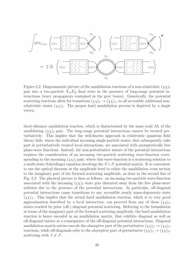
Figure 2.2: Diagrammatic picture of the annihilation reactions of a non-relativistic (χχ)Ipair into a two-particle XAXB final state in the presence of long-range potential in-teractions (wavy propagators contained in the grey boxes). Generically, the potentialscattering reactions allow for transitions (χχ)I → (χχ)J , to all accessible additional non-relativistic states (χχ)J . The proper hard annihilation process is depicted by a singlevertex.
short-distance annihilation reaction, which is characterised by the mass scale MI of theannihilating (χχ)I pair. The long-range potential interactions cannot be treated per-turbatively. This implies that the well-known approach in relativistic quantum fieldtheory fails, where the individual incoming single-particle states, that subsequently takepart in perturbatively treated local interactions, are associated with asymptotically freeplane-wave functions. Instead, the non-perturbative nature of the potential interactionsrequires the consideration of an incoming two-particle scattering wave-function corre-sponding to the incoming (χχ)I pair, where this wave-function is a scattering solution toa multi-state Schrodinger equation involving the N×N potential matrix. It is convenientto use the optical theorem at the amplitude level to relate the annihilation cross sectionto the imaginary part of the forward scattering amplitude, as done in the second line ofFig. 2.2. The physical picture is then as follows: an incoming two-particle wave-functionassociated with the incoming (χχ)I state gets distorted away from the free plane-wavesolution due to the presence of the potential interactions. In particular, off-diagonalpotential interactions cause transitions to any accessible nearly mass-degenerate state(χχ)J . This implies that the actual hard annihilation reaction, which is to very goodapproximation described by a local interaction, can proceed from any of these (χχ)Jstates reached by prior (off-) diagonal potential scattering. Referring to the formulationin terms of the imaginary part of the forward scattering amplitude, the hard annihilationreaction is hence encoded in an annihilation matrix, that exhibits diagonal as well asoff-diagonal entries as a consequence of the off-diagonal potential interactions. Diagonalannihilation matrix entries encode the absorptive part of the perturbative (χχ)J → (χχ)Jreactions, while off-diagonals refer to the absorptive part of perturbative (χχ)J → (χχ)J ′
scattering with J 6= J ′.
20
While a rigorous derivation of the relation among the annihilation amplitude and thetwo-particle scattering wave function as well as a sound derivation of the quantity referredto as annihilation matrix is postponed to later chapters, the above discussion allowsus to guess the expression for the Sommerfeld enhancement factor, that describes theenhancement (suppression) of the annihilation cross section due to attractive (repulsive)long-range potential interactions, which cannot be treated perturbatively:
S =ψ
(I) ∗J (r = 0) ΓJJ ′ ψ
(I)J ′ (r = 0)
ψ(I) ∗0 J (r = 0) ΓJJ ′ ψ
(I)0 J ′(r = 0)
. (2.8)
We have introduced the matrix Γ, that encodes physics related to the hard perturbativeannihilation rates. The N -component vector wave-function ~ψ(I) refers to a solution ofthe Schrodinger equation
(−
~∂2
2µI1 + V (r)
)~ψ(I)(~r) = E ~ψ(I)(~r) (2.9)
where µI denotes the reduced mass associated with the incoming (χχ)I pair and E
indicates a certain available non-relativistic kinetic energy. ~ψ(I)0 gives the corresponding
solution for the free case, in absence of long-range potential interactions. The potentialmatrix V encodes (off-) diagonal potential interactions, that are assumed to depend onthe radial variable r only and to vanish for r → ∞ at least as 1/r. In addition, thediagonal entries of V also incorporate effects from the constant mass splittings δMI =MI −M between the N two-particle states (χχ)I to a certain mass scale M . Becausethe potential interactions vanish for r → ∞, the potential matrix becomes diagonal inthis limit,
VIJ(r →∞)→ δMI δIJ . (2.10)
In particular, these entries are present in the equation for the free wave-function ~ψ(I)0 .
The mass scaleM in the definition of δMI =MI−M can but does not need to be chosenas the mass of the lightest state (χχ)1 out of the N -state set. In any case, however, it hasto be chosen close to the lightest state’s mass to ensure the non-relativistic nature of theset-up. Imagine for example the case of the single positive-charged sector in neutralino-chargino co-annihilations. Here it could proof useful to choose M as 2mχ0
1, the mass of
the lightest neutral state χ01χ
01 and not the (typically only slightly) larger massmχ0
1+mχ+
1
of the lightest state in the single-charged sector. In this case, the energy E in the single-charged sector’s Schrodinger equations will refer to the kinetic energy available for theχ01χ
01 state, E = mχ0
1v2 with v the velocity of each χ0
1 in the centre-of-mass of the two-particle system. The non-vanishing mass splittings contained in the diagonals of thesingle-charged sector’s potential matrices then correct to the actually available kineticenergy for each single-charged (χχ)I channel. Using such a convention for all chargesectors in χ0/χ± (co-) annihilation reactions, the same kinetic energy E = mχv
2 will
21
appear in all Schrodinger equations of the different charge-sectors. We will adapt thisconvention later and hence anticipate here the identification E = mχv
2 for the kineticenergy in the Schrodinger equation (2.9). Keep in mind, that (2.9) applies to the relativecoordinate ~r in the (χχ)I system and we have used r = |~r|. Let us first approximate(2.9) by replacing the reduced mass µI of the given incoming pair (χχ)I by the reducedmass µ ≡ mχ/2, typically referring to the lightest state (χχ)1 out of the N state set. Inthe application to neutralino and chargino co-annihilations, mχ will denote the mass ofthe lightest neutralino χ0
1. After this replacement, we arrive at a Schrodinger equation(−
~∂2
mχ1 + V (r)
)~ψ(I)(~r) = mχv
2 ~ψ(I)(~r) . (2.11)
This equation applies now to any of the possible N incoming states (χχ)I . The differenceof (2.11) with respect to (2.9) due to the replacement of the reduced mass is a higherorder effect, counting as a correction δMJmχv
2 ∼ (mχv2)2, as the mass splittings in the
N -state set are of order of the available non-relativistic kinetic energies.According to the scattering reaction with incoming (χχ)I state, that we want to
describe, the vector-function ~ψ(I) (~ψ(I)0 ) has to be a scattering solution with the following
asymptotic behaviour
ψ(I)J (r →∞) → cJI e
ikJz + fJI(θ, φ)eikJr
r, (2.12)
describing an incoming plane wave propagating along the z-direction and an outgoingscattered spherical wave.7 The coefficients cJI should be identified with δJI , if a pureincoming (χχ)I state is described, but for notational clarity, keeping track of differentcontributions, it is convenient to consider the more general case with arbitrary cJI firstand restrict to cJI = δJI later. The coefficients fJI(θ, φ) characterise the outgoingscattered spherical wave and due to the off-diagonal potentials they are in general notproportional to δJI . Recall, that the determination of the enhancement (or suppression)
7 The asymptotic form (2.12) applies in case of radial potential interactions vanishing faster than1/r in the limit r → ∞. This holds for Yukawa potentials, arising from massive mediator exchange,which is – besides Coulomb interactions from photon exchange – the relevant potential interaction inapplication to χ0/χ± pair annihilations. For Coulomb potentials (2.12) does however not apply. In ourcase Coulomb potentials can arise from photon exchange only, which implies that the 1/r potentialsexclusively arise on the diagonal of the potential matrix V (r), when written in the two-particle mass-eigenstate basis. For large values of r the matrix V (r) will then always be diagonal, containing Coulombpotential contributions as well as constant δMJ terms only: VIJ (r ≫ 0) → (δMI + αII/r) δIJ , withr chosen large enough, such that all contributions from the shorter-ranged (Yukawa) potentials arenegligible. Accounting for Coulomb potentials, the exp (ikJz) factor in (2.12) should be replaced by theincoming wave-function in presence of the Coulomb potential in the JJ component of V (r). In addition,within the expression for the spherically outgoing scattered wave in (2.12) one has to replace exp (ikJr)
by exp(i(kJr +
mχαJJ
2kJln(2kJr))
). As the derivation taking Coulomb potentials on the diagonals of
V (r) into account is completely analogous to the short-rage potential case, and in particular leads tothe same result for the enhancement factor, we will for clarity refer to the asymptotic behaviour (2.12)in the following.
22
in presence of attractive (repulsive) potential interactions via (2.8) requires the knowledge
of the scattering solutions ~ψ(I) and ~ψ(I)0 close to the origin r ∼ 0, where the short-distance
annihilation takes place. Hence we describe next, how these scattering wave-functionscan be determined.
Following the standard procedure, ~ψ(I), ~ψ(I)0 are obtained as linear combinations from
a set of basis solutions to (2.11), such that the asymptotic behaviour in (2.12) is matched.The spherical symmetry of the individual potential interactions suggests to perform aseparation of variables and construct ~ψ from
~ψ(I) =∑
l
Pl(cos θ) ~R(J)l (r) A
(I)l J (2.13)
where ~R(J)l (r) denotes a set of basis solutions to the radial Schrodinger equation for the
lth partial wave,
− 1
mχr2d
dr
(r2d~Rl(r)
dr
)+ V (r) ~Rl(r) +
1
mχr2l(l + 1)~Rl(r) = mχv
2 ~Rl . (2.14)
The A(I)l J denote the coefficients to the basis solutions ~R
(J)l that give the specific scattering
solutions ~ψ(I). A sum over the index J is implied. Finally Pl denotes the lth Legendrepolynomial and we have hence already taken advantage of the azimuthal symmetry of thescattering configurations of interest. The free scattering solutions ~ψ
(I)0 can be built in a
similar way, replacing ~R(J)l by ~R
(J)0 l as well as A
(I)l by A
(I)0 l in (2.13). The radial functions
~R(J)0 l are then obtained as solutions to (2.14), with the potential matrix V (r) replaced
by the constant diagonal matrix V (r →∞), (2.10), containing only the mass splittings.There exist 2N linearly independent solutions to (2.14) out of which N are irregular at theorigin, hence restricting us to the set of N regular solutions. The asymptotic behaviourof the Jth component of the regular linearly independent solutions ~R(I), I = 1, . . . , N ,is given by
R(I)l J (r →∞) → 1
r(nl)JI sin
(kJ r −
lπ
2+ (δl)JI
), (2.15)
with constant coefficients (nl)JI and scattering phases (δl)JI .8 Further, we have defined
8 Taking Coulomb potentials on the diagonal of the potential matrix V (r) into account, the asymp-
totic behaviour of the basis solutions ~R(I)l reads
R(I)l J (r →∞)→ 1
r(nl)JI sin
(kJr −
lπ
2+mχαJJ
2kJln(2kJr) + (δl)JI
),
with constant coefficients (nl)JI and scattering phases (δl)JI as before. The r and kJ dependent termmχαJJ
2kJln(2kJr), appearing as additional argument inside the sine, accounts for the presence of a long
range Coulomb potential −αJJ/r in the JJ component of V (r). Note that the modifications on the
asymptotic behaviour of the scattering solutions ψ(I)J (r → ∞) in (2.12) when including Coulomb-
potentials consist in the introduction of the same type of additional contributions, namely factors
exp(±i(mχαJJ
2kJln(2kJr))
), modifying the (terms in the partial-wave expansion of the) incoming plane
wave exp (ikJz) as well as the outgoing scattered spherical wave ∝ exp (ikJr)/r, see footnote 7.
23
kJ =√mχ (mχv2 + iǫ− VJJ(r →∞)) =
√mχ (mχv2 + iǫ− δMJ) . (2.16)
With the +iǫ prescription we implement our convention√−1 = +i. For completeness
and due to the slightly increased complexity in case of the matrix-valued Schrodingerequation with its vector solutions, we write here the well known procedure to determinethe scattering wave functions in terms of the basis of partial-wave solutions in (2.13).This is done in close analogy to [36]. In particular we adopt a similar notation as usedin this reference.
On the one hand side, using the expansion of the plane wave eikJz in terms of sphericalwaves, (2.12) can be rewritten as
ψ(I)J (r →∞) → eikJr
r
(cJI2ikJ
∑
l
(2l + 1)Pl(cos θ) + fJI(θ, φ)
)
− e−ikJr
r
cJI2ikJ
∑
l
(−1)l(2l + 1)Pl(cos θ) . (2.17)
On the other hand, starting from (2.13)
ψ(I)J (r →∞) → eikJr
r
(1
2i
∑
l
(−i)lPl(cos θ)ei(δl)JJ′ (nl)JJ ′ A(I)l J ′
)
− e−ikJr
r
(1
2i
∑
l
ilPl(cos θ)e−i(δl)JJ′ (nl)JJ ′ A
(I)l J ′
). (2.18)
It is convenient to establish a matrix-notation here, introducing N ×N matrices ψ andRl, that contain the scattering and regular (lth partial-wave) radial solutions in theircolumns, respectively:
ψJI(r) = ψ(I)J (r) , Rl JI(r) = R
(I)l J (r) . (2.19)
Similarly, a constant coefficient matrix Al is built, with components Al JI = A(I)l J . Even-
tually, introducing the matrix Ml with components
(Ml)JJ ′ = (nl)JJ ′ e−i(δl)JJ′ , (2.20)
we derive from the comparison of the respective second lines in (2.17) and (2.18) theexpression for the coefficient matrix
Al JI = il (2l + 1) (M−1l )JJ ′
cJ ′I
kJ ′
. (2.21)
M−1l encodes normalisations and scattering phases of the basis solutions, while the nor-
malisation of the scattering solutions for r → ∞ is assured by the dependence on the
24

coefficients cJ ′I . It is worth to note, that (2.21) as well as all following steps in our deriva-tion hold in exactly the same form for the case including Coulomb potential interactionson the diagonal of the potential matrix V (r), where in this case the normalisations andscattering phases encoded in M−1
l have to be extracted from the asymptotic behaviour
of the corresponding basis solutions R(I)l J (r →∞) as given in footnote 8.
The scattering wave-functions at the origin that appear in our guessed form (2.8) ofthe Sommerfeld enhancement factor are now obtained from the columns of the matrixψ in the appropriate limit
ψ(I)J (r → 0) = ψJI(r → 0) =
∑
l
Pl(cos θ) Rl JJ ′(r → 0) Al J ′I . (2.22)
Consequently the next step is the determination of Rl(r → 0). From the lth partial-waveradial Schrodinger equation (2.14), the behaviour Rl(r → 0) ∝ rl is inferred, supposing,that the long-range potentials in V grow less strongly than 1/r2 for r → 0. As we willconsider Coulomb and Yukawa potential interactions, this condition is fulfilled in ourcase. The usual ansatz Rl(r) = χl(r)/r allows to rewrite the radial Schrodinger equationfor the matrix-valued function χl(r)
d2
dr2χl(r) =
(l(l + 1)
r2+ mχ
(V (r)−mχv
2 1))
χl(r) , (2.23)
and the leading terms in the expansion of matrix Rl(r) around r = 0 can be expressedin terms of the (l + 1)th derivative of χl,
Rl(r → 0) = rlχ(l+1)l (r = 0)
(l + 1)!+ O(rl+1) . (2.24)
Analytic solutions to (2.23) can be found for the free case (where V (r) is given by theconstant diagonal-matrix V (r → ∞), (2.10)) as well as for a 1-state model with long-range Coulomb potential interactions. Already for the case of a Yukawa potential ina 1-state model, the equation has to be solved numerically. In the free case, relevantfor the determination of the denominator expression in the Sommerfeld enhancementformula (2.8), the radial Schrodinger equation (2.23) can be rewritten to
r2d2
dr2χ0 lJI(r) + r2 k2J χ0 lJI(r) − l(l + 1)χ0 lJI(r) = 0 . (2.25)
There is no summation over the index J in (2.25), such that a system of N decoupledequations is obtained. The free vector basis-solutions in the radial coordinate, encodedin the columns of matrix χ0 l, can hence be chosen as ~χ
(I)0 l J = χ0 lJI = δJI χ0 l, where
χ0 l denotes an ordinary, one-dimensional and in general complex valued wave-function.Using the ansatz χ0 l =
√r J0 l in (2.25), a Bessel differential equation for the function
J0 l results,
x2Jd2
dx2JJ0 l(xJ) + xJ
d
dxJJ0 l(xJ) +
(x2J − (l +
1
2)2)J0 l(xJ) = 0 , (2.26)
25

with xJ = kJ r and no summation over J . A generic solution to (2.26) is found as linearcombination of Bessel functions of the first and second kind, Jl+1/2(xJ) and Yl+1/2(xJ).
As the scattering wave-function has to be regular at xJ = 0, though, only J0 l(xJ ) =Jl+1/2(xJ) is considered. Hence the N basis solutions encoded in the matrix χ0 l can beexpressed in terms of
χ0 lJI(r) = δJI cJ√r Jl+1/2(kJ r) , (2.27)
where cJ is an arbitrarily chosen normalisation constant to the Ith basis solution. Obvi-ously, the dependence on cJ finally has to cancel out, when the free scattering solutionsare constructed. From the known asymptotic behaviour of the Bessel functions we obtainfor r →∞
R0 l JI(r →∞) =χ0 l JI(r →∞)
r
−→ 1
rδJI cJ
√2
π kJsin
(kJ r −
lπ
2
)+ O
(1
kJ r3/2
), (2.28)
as well as in the limit r → 0
R0 l JI(r → 0) −→ δJI rl cJ
(kJ / 2)l+1/2
Γ(l + 3/2)+ O
(rl+2
). (2.29)
Comparing to (2.15), the constant normalisation coefficients (nl)JI hence read in thefree case (n0 l)JI = δJI cJ
√2/πkJ , and all scattering phases vanish, (δ0 l)JI = 0. Con-
sequently (using (M−10 l )JJ ′ = δJJ ′/ cJ
√π kJ/2 ) the free case’s coefficient matrix (2.21)
reads
A0 l JI = il (2l + 1)δJJ ′
cJ
√π kJ2
cJ ′I
kJ ′
= il (2l + 1)
√π
2 kJ
cJIcJ
. (2.30)
After simple algebraic manipulations, the free scattering solutions for r → 0 are finallyobtained from
ψ0 JI(r → 0) =∑
l
Pl(cos θ) R0 l JJ ′(r → 0) Al J ′I
−→∑
l
Pl(cos θ) rl il
2l + 1
(2l + 1)!!klJ cJI . (2.31)
Let us suppose that for the interacting case with a generic potential matrix V , including(off-) diagonal long-range potential interactions, a matrix χl of solutions has been de-termined numerically from (2.23), subject to certain initial conditions, and the (l+1)th
derivative χ(l+1)l is known as well. Then the scattering solutions for r → 0 can be
generically expressed in terms of
ψJI(r → 0) =∑
l
Pl(cos θ) rl il
2l + 1
(l + 1)![χ
(l+1)l (r = 0)]JJ ′ (M
(−1)l )J ′I′ CI′I (2.32)
26

where we have introduced the matrix C, that encodes the initial conditions (2.12) forthe incoming plane-wave part of the scattering solutions, CI′I = cI′I/kI′.
Similar to the partial-wave decomposition (2.13) of the (free) scattering solutions con-tained in ψ(r) and ψ0(r), also the short-distance annihilation process can be arranged ina partial-wave expansion. In the formulation of the guessed enhancement factor in (2.8),with the configuration-space scattering wave-functions to the left and right of the quan-tity Γ, such a partial-wave expansion of the latter annihilation matrix expression involvesspatial derivatives acting on the wave-functions to its left and right. Written in radialcoordinates, the lth partial-wave contribution in particular involves the lth derivativeswith respect to the radial variable r, acting on ψ∗ and ψ in (2.8), respectively. This allowsus to refine the first guess of the formula for the Sommerfeld enhancement factor. Theenhancement of the lth partial-wave annihilation rate of the incoming scattering state(described by an incoming plane wave cJI exp(ikJz), that gets subsequently distortedby (off-) diagonal long-range potential interactions) with respect to the correspondingperturbative lth partial-wave rate is given by
SIl =ψ∗JI(r = 0) ΓJJ ′ ψJ ′I(r = 0) |l−wave
ψ∗0 JI(r = 0) ΓJJ ′ ψ0 J ′I(r = 0) |l−wave
=
((2l + 1)!!
(l + 1)!
)2
[[[χ
(l+1)l (r = 0)]M−1
l C]†· Γl ·
[[χ
(l+1)l (r = 0)]M−1
l C]]
II[klJ cJI
]∗ΓlJJ ′
[klJ ′ cJ ′I
] . (2.33)
To describe the case of a pure incoming state (χχ)I , the identification cJI = δJI , implyingCII′ = δII′/kI for the matrix C in the numerator above has to be made. (2.33) makesuse of the r → 0 behaviour of the (free) scattering solutions contained in ψ0 and ψas given in (2.31) and (2.32). The quantity Γl denotes the constant coefficient matrixencoding the hard (off-) diagonal l-wave annihilation process, that is obtained from thecorresponding appropriate partial-wave expansion of the perturbative (χχ)I → (χχ)Jamplitudes’ absorptive part.
To make use of (2.33) as it stands the combination of normalisation coefficients (nl)JIand scattering phases (δl)JI encoded in the matrixMl, (2.20), has to be known. They canin principle be extracted from the asymptotic form of the numerically determined solu-tions χl, but a separate precise determination, especially of the scattering phases, is veryhard. Fortunately, the product of matrices [χ
(l+1)l (r = 0)]M−1
l is related to quantities,that can be determined in an easier way. As a consequence, we will finally reformulate(2.33) in an even simpler form. To this purpose, let us consider the matrix χl(r) intro-duced earlier, containing the regular, linear independent solution vectors to the radialSchrodinger equation (2.23) in its columns. Following (2.24) and (2.15), the asymptoticbehaviour, that we have assigned (in absence of Coulomb potential interactions) is
χl JI(r → 0) −→ rl+1 [χ(l+1)l (r = 0)]JI(l + 1)!
+ O(rl+2) , (2.34)
χl JI(r →∞) −→ (nl)JI sin(kJ r −lπ
2+ (δl)JI) . (2.35)
27
The overall normalisation of the basis solution contained in χl is fixed by yet to defineinitial conditions. A convenient choice in particular for numeric solutions is related toconditions on χl in the r → 0 limit: by assigning appropriate values to χ
(l+1)l (r = 0)
the r → 0 behaviour of the regular solutions (2.34) is fixed. For the time being we canleave the question of the initial condition for the regular solutions open and come backto this point later. In addition to the matrix χl let ηl(r) be the matrix with the irregularsolutions to (2.23) with the asymptotic form
ηl JI(r → 0) −→ δJI r−l , (2.36)
ηl JI(r →∞) −→ TlJI e−i kJ r , (2.37)
such that the irregular solutions asymptotically correspond to purely incoming sphericalwaves.9 Tl denotes a hermitian coefficient matrix with in general non-vanishing off-diagonal entries. The normalisation of the basis solutions in ηl is fixed by the initialcondition that is implicit in (2.36). Due to the hermiticity of the potential matrixV †(r) = V (r), the Schrodinger equation is hermitian itself, such that the matrices χ†
l
and η†l are solutions to the hermitian conjugate radial Schrodinger equation
d2
dr2ξ†l = ξ†l
[l(l + 1)
r2+ mχ
(V (r)−mχv
2 1)]
, (2.38)
with ξl = χl, ηl. As a direct consequence it is easily seen that the generalisation of theWronskian,
Wl(r) = η†l ·(d
drχl
)−(d
drη†l
)· χl (2.39)
is constant in r, d/drW (r) = 0.10 We can hence equate
Wl(r = 0)JI =2l + 1
(l + 1)!
[χ(l+1)l (r = 0)
]JI
, (2.40)
with
Wl(r →∞)JI = il Tl†JI′ kI′ (Ml)I′I . (2.41)
This allows to obtain the relation[[χ
(l+1)l (r = 0)]M−1
l
]JI
= il(l + 1)!
2l + 1Tl
†JI kI . (2.42)
9Coulomb potential interactions from photon exchange on the diagonal of the potential matrix V (r)change the asymptotic behaviour for r →∞ in (2.35) and (2.37). In both cases we have to replace kJrby kJr +mχαJJ/2kJ ln(2kJr) (also see footnotes 7 and 8).
10 Note that (2.39) is a generalisation of the expression Wl considered in [36]. In this reference thepotential matrix was considered to be real-symmetric, such that the transpose of the matrix η, ηT ,appears in the corresponding expression Wl defined therein, instead of the hermitian conjugate η†. Dueto the generic hermiticity property of the Schrodinger equation, the definition of Wl with hermitianconjugates, (2.39), looks more natural even in the case with real-symmetric potentials.
28
Our final expression for the enhancement in the annihilation of the lth partial-wavecomponent, (2.33), subject to an incoming (χχ)I state, hence assumes the followingcompact form
SIl = ((2l − 1)!!)2
[Tl · Γl · T †
l
]II
k2lI Γl II, (2.43)
where we use the double factorial (2l − 1)!! =∏l−1
i=1(2i + 1). Note that kI is alwaysreal, as it corresponds to the momentum of the particles in the incoming scattering state(χχ)I . Equation (2.43) is consistent with the corresponding result in [36], although T ∗
appears in the reference’s formula instead of T as in (2.43). However, [36] considereddifferent irregular solutions, with asymptotically outgoing (instead of incoming, (2.37))spherical wave behaviour, while the formulation of the corresponding generalisation ofthe Wronskian Wl referred to the transposed instead of the hermitian conjugate of theirregular-solution matrix (see footnote 10). The definition of matrix T in (2.37) henceagrees with T ∗ in [36].
Thanks to the constant Wronskian Wl, the matrix Tl, related to the irregular lthpartial-wave solutions, can be calculated from the regular solutions contained in χl only.Without making use of the asymptotic form of the regular solutions in (2.35), we obtain
Wl(r →∞)JI −→ T †l JJ ′ e
i kJ′r
(d
drχl J ′I(r) − i kJ ′ χl J ′I(r)
) ∣∣∣r→∞
=[T †l · Ul(r →∞)
]JI
, (2.44)
where the matrix Ul(r) is defined by the first line above,11
Ul JI(r) = ei kJr(d
drχl JI(r) − i kJ χl JI(r)
). (2.45)
It is now convenient to choose the initial condition for the regular solutions such that[χ
(l+1)l (r = 0)]JI = (l + 1)!/(2l + 1) δJI , which implies Wl(r = 0)JI = δJI , the matrix Tl
in (2.43) is obtained from
T †l = U−1
l (r →∞) . (2.46)
As a check of (2.43) let us consider the free-case, where we should reproduce SIl = 1. Wecould either directly determine the irregular solutions for the free case or calculate Tlfrom (2.46). Choosing the latter option, we consider the free regular solutions χ0 lJI(r)in (2.27), with normalisation
cl J =
√2
π(2l − 1)!!
1
kl+1/2J
, (2.47)
11Note that the exponential factor exp(ikJr) in both (2.44) and (2.45) should be replaced byexp (i(kJr +mχαJJ/2kJ ln(2kJr))), when Coulomb potential interactions from photon exchange onthe diagonal of potential matrix V (r) are taken into account (see footnotes 7 and 8).
29
such that the correct r → 0 behaviour [χ(l+1)l (r = 0)]JI = (l+1)!/(2l+1) δJI is obtained.
Building UlJI(r) as in (2.45), we obtain
T0 l†JI = U−1
0 l JI(r →∞) =(−i)l klJ(2l − 1)!!
δJI , (2.48)
such that
[T0 l · Γl · T †
0 l
]II
= T0 lIJ ΓlJJ ′ T ∗0 lIJ ′ =
(1
(2l − 1)!!
)2
k2lI ΓlII . (2.49)
Taken together with the prefactor and denominator in (2.43), we consistently recoverSIl = 1 for the free case.
In generic practical applications, where the Schrodinger equation (2.23) generallyhas to be solved with numerical methods, the strategy in the determination of SIl is asfollows:
(1) Determine the matrix χl, containing in its columns the N regular basis solutionsto (2.23), subject to the initial conditions
[χl(r = r)]JI = r l+1 δJI2l + 1
. (2.50)
r has to be chosen close to zero, such that the solutions will obey [χ(l+1)l (r = 0)]JI =
(l + 1)!/(2l + 1) δJI , which we imposed above in order to have WlJI(r) = δJI .
(2) With the matrix χl known, build the matrix Ul(r), (2.45). To catch the asymp-totic constant behaviour of Ul(r), a large enough r∞ has to be chosen in order todetermine the constant matrix T †
l from (2.46).
(3) Supposing the annihilation matrix Γl, encoding the perturbative (off-) diagonal an-nihilation rates of the lth partial-wave states is known, calculate the enhancementfactor SIl for the incoming (χχ)I pair from (2.43).
There are numerical issues related to the solutions of the Schrodinger equation for amulti-state system, that are delicate and require application of sophisticated methods.We discuss the origin of the numerical problems and describe an improved method for thenumerical determination of the Sommerfeld enhancement factors, that solves the issue,when applying the formalism developed here to multi-state systems of χ0/χ± pairs. Thetechnical details of this improved method are postponed to Chap. 8.4, although the datatables for the plots presented throughout the thesis rely on the improved version. Inthis chapter we will continue with simple one- and two-state toy models, in order toillustrate the Sommerfeld effect and to make ourselves familiar with generic propertiesof the enhancement in presence of Coulomb or Yukawa potentials.
30
2.3 N = 1 state models with Coulomb and Yukawa
potential interactions
Before we enter a brief discussion on the well known enhancement due to Coulomband Yukawa potential interactions in models with only one single χχ state, let us firstdeduce the general form of the N = 1 state enhancement factor Sl from the genericN -state system expressions (2.33) and (2.43). Starting from (2.33), the enhancementfactor for the single χχ state case reduces to
Sl =
((2l + 1)!!
(l + 1)!
)2
∣∣∣χ(l+1)l (r = 0)/nl
∣∣∣2
k2l+2=
((2l + 1)!!
l!
)2
∣∣∣R(l)l (r = 0)/nl
∣∣∣2
k2l+2, (2.51)
with Rl(r) = χl(r)/r as usual. χl(r) is now the solution to the single state radialSchrodinger equation as obtained from (2.23) for N = 1. The asymptotic behaviourof χl and Rl follows from (2.35), (2.34) and (2.15), (2.24), respectively. nl denotesthe normalisation of the regular solution χl(r) in the r → ∞ limit. The linearity ofthe Schrodinger equation allows us to deliberately rescale any solution χl → χl = c χl,with a constant factor c, implying nl → nl = c nl. The effect of such a rescaling willin particular cancel in the enhancement formula (2.51).12 The quantity k is given byk = mχv, with mχ twice the reduced mass of the two-particle state, and v half the(asymptotically free) incoming χχ state’s relative velocity. If the χχ state is built fromequal mass constituents, mχ obviously agrees with the corresponding single particle massand v gives the modulus of the single particle velocity subject to the asymptotically freeincoming states. Just as the kJ in the N -state case, k hence generically indicates themodulus of each single particle’s momentum in the centre-of-mass of the (asymptotic)incoming χχ system. It is interesting to note, that the dependence on the scatteringphases δl cancels in the N = 1 state Sommerfeld factor, (2.51), as opposed to the genericN -state case, where each component χlJI(r) of the matrix encoding the regular radialsolutions can come with a different phase in its r →∞ behaviour. In general, the matrixproduct in (2.33) will imply no cancellation of scattering phases. Further note, that thel-wave enhancement factor Sl in the one-state case, (2.51), only relies on the potentialinteraction and is independent of the hard annihilation rate. This no longer holds true inthe general multi-state case, where a generic annihilation matrix ΓIJ with non-vanishingoff-diagonals encodes the short-distance annihilation part of the full process: while thedenominator of SIl , (2.33) or (2.43), is proportional to the perturbative hard l-waveannihilation rate of the (χχ)I state, encoded in ΓlII , the numerator, to the contrary, willgenerally contain terms involving the hard (off-) diagonal l-wave rates ΓlJJ ′ of any states(χχ)J , (χχ)J ′ accessible from the initial (χχ)I by potential scattering.
Imposing an asymptotic normalisation nl =√
2/π on the radial solution χl, we re-cover in (2.51) the l-wave enhancement formula that can be inferred from the results
12Note that the same argument applies to a global rescaling of the matrices χl and Rl in the N -statecase.
31
presented in [37] (see Eq. (3.11) and (5.1) therein). The author of [38] independentlyderived an equivalent result for the l-wave enhancement in a single state system (see Eq.(21) therein), which we reproduce by selecting the regular solution χl(r) with normali-sation nl = 1/k for r →∞.
Another equivalent form of the single χχ state enhancement factor Sl derives from(2.43),
Sl = ((2l − 1)!!)2|Tl|2k2l
, (2.52)
where Tl denotes the normalisation of the irregular solution ηl(r →∞)→ Tl exp (−ikr),with ηl(r → 0) → r−l. Tl can either be determined directly from solving for ηl, or,equivalently, from the r → ∞ behaviour of the regular solution χl (with χl(r → 0) →1/(2l + 1) rl+1) as given by the relations (2.45) and (2.46).
Unless it happens to be suppressed, the perturbative leading order S-wave χχ anni-hilation-rate constitutes the dominant contribution to the total annihilation rate of non-relativistic χχ pairs. Consequently the leading order S-wave enhancement associatedwith Sl=0 has been studied extensively in the recent literature, while higher partialwaves were in first approximation legitimately neglected as higher-order effect (with theperturbative l-wave rate scaling with a factor v2l, with v the non-relativistic velocity ofeach incoming χ particle). The authors of [29] discuss the case of l = 0 wave enhancementfor a single χχ state and give the corresponding Sl=0 factor subject to a regular solutionswith χl=0(r → ∞) → sin(kr + δl), implying nl=0 = 1 in (2.51). The same expressioncan be found in [39]. Sl=0 written in terms of irregular solutions ρl=0 with ρl=0(r →∞) ∝ exp(ikr) is given in [29] and [40]. The enhancement is said to be Sl=0 = |ρl=0(r →∞)|2/|ρl=0(r = 0)|2. This is in agreement with (2.52). First note, that our initialcondition on the irregular solution ηl=0(r), implies ηl=0(r = 0) = 1. Hence (2.52) forl = 0 is equivalent to Sl=0 = |η(r → ∞)|2/|η(r = 0)|2. As it should be, any rescalingof the irregular solution ηl=0(r) → c ηl=0(r) will hence leave the enhancement factorunchanged. From the r → ∞ behaviour, we obtain η∗l=0(r) ∝ ρl=0(r), such that finallythe same l = 0 enhancement factor expression as given in [29] and [40] results.
Let us conclude with the remark that recent literature on the Sommerfeld enhance-ment for one-state χχ dark-matter systems focused on Yukawa potential interactions,which in particular applies to the references [29, 39, 40] above. This is of course relatedto the fact that the dark matter candidate has to be both electric and colour neutral,excluding Coulomb potential interactions from photon or gluon exchange. Assuming thedark-matter candidate together with a mediator – which causes potential interactionsin the non-relativistic χχ system – to be part of a dark sector, also here the most gen-eral ansatz is to consider a massive mediator giving rise to a Yukawa potential. Theenhancement due to a Yukawa potential exhibits additional so called zero-energy reso-nances, that can lead to even stronger enhancements compared to the Coulomb case.In the next two subsections we will discuss the characteristics of the enhancement fromCoulomb and Yukawa potentials in the single χχ-state case.
32
2.3.1 One-state model with Coulomb potential
χχ scattering in a Coulomb potential is among the few cases that allow to derive an exactanalytic expression for the enhancement factors Sl. Let us sketch the steps, familiar fromquantum mechanics, that lead to the determination of the regular partial-wave solutionsχl(r) to the corresponding radial Schrodinger equation,
d2
dr2χl(r) =
(l(l + 1)
r2− mχ
α
r− k2
)χl(r) , (2.53)
which finally allow to determine the Coulomb l-wave enhancement factor. Positive (neg-ative) α = g2/4π in (2.53), with g the coupling responsible for the Coulomb potentialinteraction, refers to the case of an attractive (repulsive) potential. We will apply (2.52),by extracting the constant factor Tl from the asymptotic r →∞ behaviour of the regularsolutions χl(r) with χl(r → 0) → 1/(2l + 1)rl+1. In order to determine χl(r) we makethe well-known ansatz
χl(r) = c rl+1 eikr ωl(r) , (2.54)
with constant c to be determined such that the above imposed χl(r → 0) behaviour ismatched. The function ωl(r) interpolates between the r → 0 and r → ∞ behaviour ofthe solution χl(r), that is described by the rl+1 term and the outgoing spherical waveexp (ikr), respectively. The resulting differential equation for ωl(r) can be written asKummer differential equation for wl(z),
z ω′′l + (2l + 2− z)ω′
l(z)−(l + 1− i mχα
2k
)ωl(z) = 0 , (2.55)
with z = −2ikr. The solutions regular at r = 0 are the confluent hyper-geometricfunctions 1F1(l + 1 − imχα/2k, 2l + 2,−2ikr). Choosing the right r → 0 normalisation,we find the regular solutions to (2.53) as
χl(r) =1
2l + 1rl+1 eikr 1F1(l + 1− imχα/2k, 2l + 2,−2ikr) . (2.56)
In order to extract Tl we need the asymptotic r →∞ behaviour of the confluent hyper-geometric functions. The latter is found from
1F1 (a, b, |z| → ∞) =Γ(b)
|Γ(a)|(eiη (−z)−a + e−iη+z za−b
), (2.57)
with η defined as Γ(a) = eiη |Γ(a)|. After some algebraic manipulations, this allows usto obtain
χl(r →∞) =(2l)! e−πmχα/4k
2l kl+1 Γ(l + 1− imχα
2k)sin
(kr − lπ
2+mχα
2kln(2kr) + η
). (2.58)
33
Hence, following (2.45) with the appropriate replacement of the factor exp(ikJr) byexp [i(kr +mχα/2k ln(2kr))] for the Coulomb case,
Ul(r) = ei(kr+mχα
2kln(2kr))
(d
drχl(r) − ik χl(r)
)
=il eiη (2l)! e−πmχα/4k
2l kl Γ(l + 1− imχα2k
)+O
(1
r
), (2.59)
such that for the one-state case we obtain from (2.52), with T † = T ∗ = U−1(r →∞),
Sl = 22l((2l − 1)!!
(2l)!
)2 ∣∣∣∣Γ(l + 1− imχα
2k
)∣∣∣∣2
eπmχα/2k
=πα/v
1− e−πα/vl∏
j=1
(1 +
(α/v)2
4j2
). (2.60)
In the last step we have used Γ(x + 1) = xΓ(x), the property Γ(x∗) = Γ(x)∗ and therelation Γ(1 + ix)Γ(1 − ix) = πx/ sinh(πx) for real x. Finally, k = mχv allowed us toexpress the Coulomb l-wave enhancement factor in terms of the fraction α/v only.
In the limit v ≫ |α| we have Sl → 1 for both the attractive (α > 0) and repulsive(α < 0) case, as expected. For the attractive case, for very low velocities v ≪ α, theenhancement factor scales as Sl → π(α/v)2l+1/ (22l l!2). In the leading order S-wave(l = 0) case we hence recover the familiar πα/v behaviour of the Coulomb enhancementfor v/α≪ 1. Since the perturbative l-wave annihilation rate σ0
l vrel has a velocity depen-dence proportional to v2l, the corresponding Sommerfeld enhanced rate σlvrel = Slσ
0l vrel
exhibits a 1/v velocity dependence for v/α → 0, which is in particular the same forall l-waves. Higher Sommerfeld enhanced l-wave rates are however suppressed by theconstant factor 1/l!2 (α/2)2l, that arises in the product v2lSl → πα/v × 1/l!2 (α/2)2l.For v/α → 0, the enhanced leading order S-wave rate will hence dominate the annihi-lation and higher l-waves can be safely neglected. As long as moderate velocities areconsidered, for example v ∼ 1/3 as around freeze-out of a cold dark-matter candidate,the v2 proportional perturbative P -wave rate possibly gives corrections to the leadingperturbative S-wave rate at the level of some percent. Since in the attractive case the en-hancement factor Sl, (2.60), obviously increases with increasing l, P -wave enhancementsshould consequently be considered in an accurate percent level calculation of annihilationrates, where the particle velocities are of order O(0.1). This provides us with the moti-vation to study the effect of Sommerfeld enhancements on neutralino and chargino (co-)annihilation rates including P - and up to O(v2) S-wave enhancements in application tothe χ0
1 relic abundance calculation.To conclude, consider the repulsive case (α < 0). In the v/|α| → 0 limit, we obtain
the familiar exponential suppression Sl ∝ exp(−π|α|/v), resulting from the need topenetrate the Coulomb barrier. Besides the exponential suppression, the l > 0 waverates will be in addition reduced with respect to the l = 0 case by the same constant1/l!2 (α/2)2l factor as in the attractive case.
34
2.3.2 One-state model with Yukawa potential
In the case of a Yukawa potential V (r) = −α exp(−mφ r)/r, with α > 0 (α < 0) refer-ring to an attractive (repulsive) interaction, the mediator mass mφ gives an additionalparameter in the Schrodinger equation and causes the potential to be short-ranged (inthe sense that it vanishes faster for r →∞ as ∝ 1/r−1 due to the exponential suppressionfactor). We will restrict to the more interesting attractive case α > 0 throughout thissection, as we are primarily interested in the enhancement rather than the suppression ofannihilation rates.13 After rescaling the radial coordinate r in the one-state Schrodingerequation by a factor αmχ, the latter contains the two dimensionless parameters
ǫv =v
α, ǫφ =
mφ
αmχ, (2.61)
only. mχ denotes the common mass of the particles χ, that build up the χχ one-statesystem under consideration and v is the single-particle velocity in the centre-of-massframe. From the discussion in Sec. 2.1 we can expect two regions in the ǫv − ǫφ planewith different characteristics of the enhancement Sl(ǫv, ǫφ). Considering the momentum-space propagator of the t- or u-channel exchanged mediator in the potential region,1/(~k2+m2
φ) ∼ 1/(m2χv
2+m2φ), we can neglect the mediator mass as long as mφ ≪ mχv.
This condition is equivalent to ǫφ ≪ ǫv, and in the corresponding region the enhancementis expected to be Coulomb-like. On the other hand, for mχv ≪ mφ, but still mφ ≪ mχ,the potential derived from the mediator exchange becomes constant, leading to a velocityindependent enhancement in the region ǫv ≪ ǫφ. There is an additional effect in theǫv < ǫφ region leading to extra sizable enhancements, that is specific to finite rangepotentials: the presence of so called “zero-energy resonances”. There exists a finitenumber of bound states for a finite range potential. By varying the dimensions of such apotential – in case of the one-state Yukawa potential encoded in the parameter ǫφ – onecan arrange for a bound state with zero-energy. If such a zero-energy bound state exists,the scattering of an incoming state with single-particle velocity v close to zero becomesresonant. Such a behaviour, leading to strong resonant enhancements, is familiar fromquantum mechanical scattering, for example scattering at an attractive potential well.The resonant enhancement can be already strong, if a loose, but not exactly zero-energybound state exists in the spectrum of the system.
Although the Schrodinger equation for the Yukawa potential has to be solved nu-merically, an analytic approximation can be obtained by replacing the Yukawa by theso called Hulthen potential [38]. This allows to get some insight into the enhancementespecially in the resonance region. The Hulthen potential shows the same short- andlong-distance behaviour as the Yukawa potential and is of the form
VH(r) = − α δ e−δr
1− e−δr . (2.62)
13As a side-remark note that the case of suppression of annihilation rates due to repulsive potentialswill arise in the MSSM application in the double charged sector of χ±χ± systems. This effect, though,turns out to play a sub-dominant role in the χ0
1 relic abundance calculation, which constitutes our majorconcern in this work.
35
The parameter δ should be chosen such, that the Yukawa potential case with V (r) =−α exp(−mφ r)/r is mimicked with sufficient accuracy. A convenient criterion fixing δcan be obtained from the Lippmann-Schwinger equations, which determine the radialsolutions Rl(r) = χl(r)/r in presence of the Yukawa or Hulthen potential as a series inthe corresponding potential interaction. Relying on this criterion, δ is fixed in [38] by thecondition that the radial solutions Rl(r) in presence of the Yukawa and Hulthen potentialinteractions agree to first order in α in the ǫv → 0 limit. This implies
∫∞0dr r V (r) =∫∞
0dr r VH(r) and yields δ = π2mφ/6. The Hulthen approximation to the Yukawa
potential case becomes worse for finite kinetic energy (ǫv > 0). Yet, as we will see below,imposing the above matching criterion that fits the parameter δ, the analytic Sommerfeldenhancement expression obtained for the Hulthen approximation reproduces the numericresult in the Yukawa case with ǫv > 0 within ∼ 10% accuracy. The l = 0 enhancementformula derived from [38] and quoted for example in [36, 40] reads
SHull=0 =
π
ǫv
sinh(
2πǫvǫφ
)
cosh(
2πǫvǫφ
)− cos
(2π√
1ǫφ− ǫ2v
ǫ2φ
) , (2.63)
where we have defined ǫφ = π2/6 ǫφ. A similar expression for l > 0 waves is obtainedeasily from [38], adding additional factors to the SHul
l=0 term above. As the agreementbetween this Hulthen potential approximation to the Yukawa case becomes worse forhigher partial waves we do not give the expressions here. For a discussion on the pooreragreement see [38]. From (2.63) we can see, that for an attractive potential (α > 0) andǫv ≪ ǫφ, resonances arise in the S-wave case if
mφ =6α
π2 n2mχ , n = 1, 2, . . . . (2.64)
A similar relation holds for the higher (l > 0) partial waves, with n above replacedby n = l + 1, l + 2, . . .. This is a specific feature of the Hulthen potential and doesin particular not hold for the Yukawa potential case. In the latter case the resonancepositions of different l-waves do not coincide.14 For mφ given by (2.64), the enhancementSHull=0 in the small v region is given by
SHull=0(ǫv → 0, ǫφ = 6/πn2) −→ π2 αmφ
6 v2mχ, (2.65)
hence scaling as v−2, which gives rise to a much stronger enhancement compared to theCoulomb v−1 behaviour.15 Note that despite the resonance positions being shifted incase of the Yukawa potential, the on-resonance v−2 scaling in (2.65) also applies to theYukawa case.
We exemplify the features of the S-wave Sommerfeld enhancement in presence ofYukawa and Hulthen potentials in Fig. 2.3 and Fig. 2.4. The ǫv-dependence of the
14It was argued in [38], that due to the non-coincidence of resonance positions of different l-waves ina Yukawa potential a process could be dominated by a higher than l = 0 partial wave, if taking placeon a resonance of a l > 0 partial wave.
15The v−2 scaling of Sl(ǫv, ǫφ) at a resonance is generic also for the l > 0 partial waves.
36
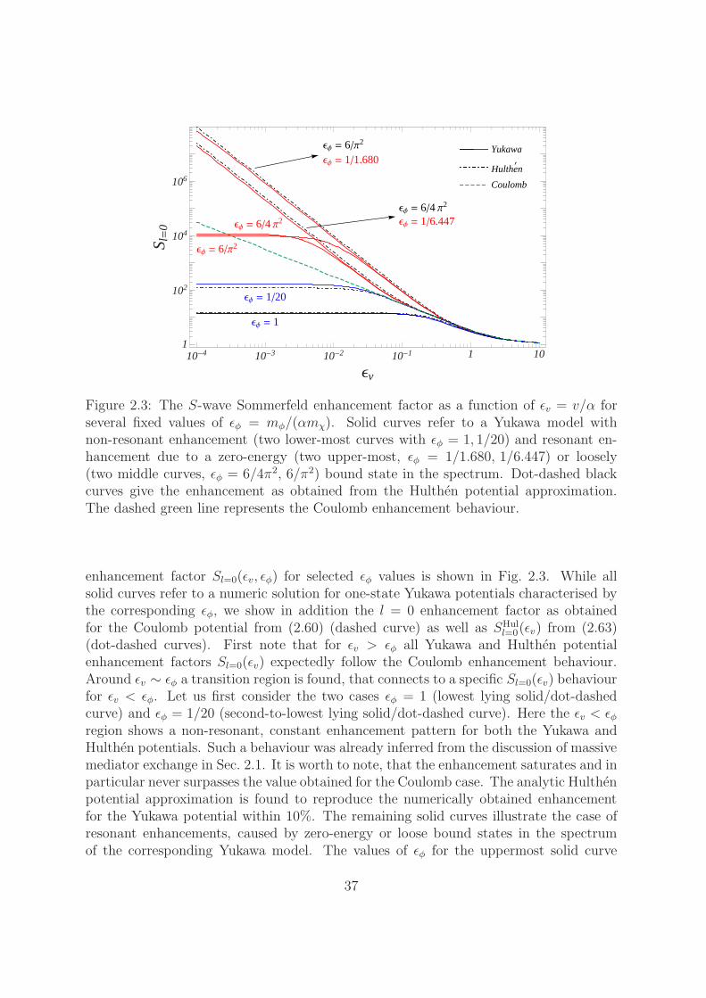
10-4 10-3 10-2 10-1 1 101
102
104
106
Εv
S l=
0
ΕΦ = 1
ΕΦ = 120
ΕΦ = 6Π2
ΕΦ = 64 Π2
ΕΦ = 64 Π2
ΕΦ = 16.447
ΕΦ = 6Π2
ΕΦ = 11.680Yukawa
Hulthe¢n
Coulomb
Figure 2.3: The S-wave Sommerfeld enhancement factor as a function of ǫv = v/α forseveral fixed values of ǫφ = mφ/(αmχ). Solid curves refer to a Yukawa model withnon-resonant enhancement (two lower-most curves with ǫφ = 1, 1/20) and resonant en-hancement due to a zero-energy (two upper-most, ǫφ = 1/1.680, 1/6.447) or loosely(two middle curves, ǫφ = 6/4π2, 6/π2) bound state in the spectrum. Dot-dashed blackcurves give the enhancement as obtained from the Hulthen potential approximation.The dashed green line represents the Coulomb enhancement behaviour.
enhancement factor Sl=0(ǫv, ǫφ) for selected ǫφ values is shown in Fig. 2.3. While allsolid curves refer to a numeric solution for one-state Yukawa potentials characterised bythe corresponding ǫφ, we show in addition the l = 0 enhancement factor as obtainedfor the Coulomb potential from (2.60) (dashed curve) as well as SHul
l=0(ǫv) from (2.63)(dot-dashed curves). First note that for ǫv > ǫφ all Yukawa and Hulthen potentialenhancement factors Sl=0(ǫv) expectedly follow the Coulomb enhancement behaviour.Around ǫv ∼ ǫφ a transition region is found, that connects to a specific Sl=0(ǫv) behaviourfor ǫv < ǫφ. Let us first consider the two cases ǫφ = 1 (lowest lying solid/dot-dashedcurve) and ǫφ = 1/20 (second-to-lowest lying solid/dot-dashed curve). Here the ǫv < ǫφregion shows a non-resonant, constant enhancement pattern for both the Yukawa andHulthen potentials. Such a behaviour was already inferred from the discussion of massivemediator exchange in Sec. 2.1. It is worth to note, that the enhancement saturates and inparticular never surpasses the value obtained for the Coulomb case. The analytic Hulthenpotential approximation is found to reproduce the numerically obtained enhancementfor the Yukawa potential within 10%. The remaining solid curves illustrate the case ofresonant enhancements, caused by zero-energy or loose bound states in the spectrumof the corresponding Yukawa model. The values of ǫφ for the uppermost solid curve
37

10-2 10-1 1 101
10
102
103
104
105
106
ΕΦ
S l=
0
Εv = 1
Εv = 10-1
Εv = 10-2
Εv = 10-3
Εv = 10-3
HHulthe¢n approx.L
Figure 2.4: The S-wave enhancement factor in a one-state Yukawa model (solid lines)as a function of ǫφ = mφ/(αmχ) for selected constant values of ǫv = v/α. The dashedcurve gives the approximate enhancement factor as obtained from a Hulthen potentialwith constant ǫv = 10−3.
(ǫφ = 1/1.680) as well as the second solid curve from above (ǫφ = 1/6.447) are taken from[41] and correspond to the numerically determined first two critical values, that implythe existence of a l = 0 zero-energy bound state in the spectrum of the Yukawa model.The corresponding dot-dashed curves, following closely the Yukawa cases, correspond tothe SHul
l=0 solutions with ǫφ = 6/π2 ≈ 1/1.645 and ǫφ = 6/4π2 ≈ 1/6.580, respectively.The latter correspond to the first two ǫφ values that are associated with a zero energybound state in the Hulthen potential, see (2.64). The Hulthen approximation hencepredicts the ǫφ associated with zero-energy resonances within an accuracy of 2% in bothcases considered here. The two solid curves with ǫφ = 6/π2 and ǫφ = 6/4π2 that followthe above-discussed Yukawa-potential resonance curves for ǫv > 3 · 10−2, but approacha constant enhancement for smaller values of ǫv correspond to Yukawa potentials withloose but not exactly zero-energy bound states. The fact that the enhancement factorsfor these two cases approach values Sl=0(ǫv → 0) of the same order of magnitude ispurely accidental. Generically, small variation of ǫφ around a resonance value, implyingthe presence of a loosely-bound state, will give rise to significantly different constantvalues Sl=0(ǫv → 0). As can be seen from Fig. 2.3, the presence of loosely-bound statescan lead to enhancements, that are several orders of magnitude stronger as comparedto the non-resonant case. Depending on the considered value of the velocity it caneven be stronger than in the Coulomb case, as a consequence of the v−2 proportionalityof the resonant enhancement. This latter v−2 scaling-behaviour holds for the loosely-
38

bound states in the ǫv < ǫφ regime as long as the kinetic energy of the scattering stateis significantly larger compared to the loosely-bound state’s binding energy; the latterstate can then be effectively considered as zero-energy bound state. Finally note thatdespite the formal v−2 divergence of the resonant enhancement (2.65) as v → 0, thephysical enhancement is finite on resonance due to the finite width of the zero-energytwo-particle bound state. The latter width is however not taken into account in thequantum mechanical treatment of the scattering process that we have applied here.
The l = 0 wave enhancement factor for a Yukawa-model as a function of ǫφ is shownin Fig. 2.4, where we have fixed ǫv = 1, 10−1, 10−2, 10−3. The emergence of resonances forǫφ > ǫv at specific ǫφ values is apparent. The first two resonance positions are found atǫφ = 1/1.680 and 1/6.447 in agreement with [41]. For ǫφ < ǫv, resonances are expectedlyabsent in Fig. 2.4 and with further decreasing ǫφ the enhancement factor matches theCoulomb one for the corresponding ǫv value. For comparison, the enhancement factoras obtained for a Hulthen potential with ǫv = 10−3 is shown in addition (dashed curve).While the approximation agrees with the Yukawa case at the level of a few percentaround the first resonances, we find, that it reproduces the latter at the 10% level onlyfor smaller ǫφ values, in agreement with the results in [38, 40].
2.4 A two-state model with off-diagonal interactions
The next straightforward step in increasing the complexity of our toy-models impliesconsidering more two-particle states (χχ)I . Another direction would be to change thenumber of potentials in the one-state case, allowing several mediators with differentmasses as well as different coupling strength to the constituents of the single χχ pair.Such kind of investigations have been carried out in [42] or [43]. We pursue the firstoption and consider the case of a two-state system with states (χχ)I , I = 1, 2, thattake part in purely off-diagonal potential interactions through exchange of one singlemassive mediator with mass mφ. The two states shall exhibit a small mass difference,δM2 =M2−M1 > 0, where MI denotes the mass of the state (χχ)I . A very comprehen-sive study of the enhancements arising for the lighter two-particle state (χχ)1 in such aninelastic two-state model, including approximate analytic formulae, can be found in [36].Here we will present results for the Sommerfeld enhancement obtained from numericallysolving the Schrodinger equation for the coupled two-state system, highlighting the qual-itative features of the enhancement. For an elaborate discussion including approximateanalytical results the reader is referred to [36].
We assume that written in the mass-eigenstate basis of the two two-particle states(χχ)1, (χχ)2, the potential matrix V (r) has the following form,
V (r) =
0 −αre−mφr
−αre−mφr δM2
. (2.66)
It is convenient to use the dimensionless quantities ǫv = v/α and ǫφ = mφ /αmχ, asgiven in (2.61). mχ denotes twice the reduced mass of the lighter state (χχ)1. (In
39

most applications mχ is hence the mass of the single-particle constituents in (χχ)1.) Inaddition we introduce the new parameter ǫδ =
√δM2/α2mχ, associated with the mass
splitting in the two-state system.The potential matrix (2.66) in this purely inelastic two-state system resembles the
leading order 1S0-wave potential in the neutral sector of pair-annihilating wino-likeχ01 dark-matter. The latter neutral sector features the two nearly mass-degenerate
two-particle states χ01χ
01, χ
+1 χ
−1 . Off-diagonal potential scattering χ0
1χ01 → χ+
1 χ−1 and
χ+1 χ
−1 → χ0
1χ01 is mediated by W -exchange. For heavy χ0
1, χ±1 particles, mχ ∼ O(TeV),
the mass splitting between the neutral two-particle states in the decoupling limit isgiven by δMwino
2 ∼ 300MeV, independent of the wino-masses (as well as of the (de-coupled) residual SUSY spectrum). The features of gaugino- as well as higgsino-likeχ01 dark-matter, including mass splittings, will be discussed in detail in later chapters.
For the time being note that purely off-diagonal potential scattering generically arisesfor two-particle states built from one single Majorana fermion state (as for example theχ0iχ
0i states in the MSSM), if the potential interactions are mediated by gauge bosons;
Majorana fermions cannot carry conserved charges, implying purely off-diagonal poten-tial (χχ)I → (χχ)J 6=I scattering reactions to accessible nearly mass-degenerate states(χχ)J 6=I . In that sense the ansatz (2.66) for the potential interactions is generic for atwo χχ-state system, with the lighter state, (χχ)1, built from a Majorana dark-mattercandidate. The above reasoning pertaining to purely off-diagonal potential scatteringdoes however not apply to (χχ)I states built from Dirac fermions, as for example χ+
1 χ−1
in the system of neutral wino-states. The major difference between (2.66) and the 1S0
potential interactions in the neutral sector of pair-annihilating non-relativistic winos ishence the fact, that the χ+
1 χ−1 state allows for diagonal potential interactions mediated
by photon- and Z-exchange. These potentials will then appear in the (2, 2) componentof the corresponding potential matrix, in addition to the mass splitting δM2 as in (2.66).
In the generic case, there exists no r-independent diagonalisation of the two-stateSchrodinger equation over the complete range of r, given the potential matrix V (r) in(2.66). Depending on the actual magnitude of the parameters ǫφ and ǫδ, there will betwo regions, where the potential interaction −α/r exp(−mφr) dominates over the masssplitting and vice versa, separated by a transition region, where both the interaction andthe mass splitting are of the same order.
It is instructive to first consider in a bit more detail the leading order S-wave Som-merfeld enhancement for both states (χχ)I=1,2 in case of vanishing mass splitting, ǫδ = 0,as in this case an r-independent diagonalisation of the two-state Schrodinger equationis possible and we can in addition gain some insight into the relevance of off-diagonalannihilation rates in the determination of SIl . Let us rewrite the Schrodinger equationfor the matrix valued function χl(r) in the following form
d2
dx2χl(x) =
l(l+1)x2− ǫ2v −e
−ǫφx
x
−e−ǫφx
xl(l+1)x2− ǫ2v + ǫ2δ
χl(x) , (2.67)
where we have introduced the rescaled radial coordinate x = αmχr, and ǫδ should
40
be set to 0 for the time being. The eigenvalues and the corresponding r-independenteigenvectors of the matrix multiplying χl(x) on the r.h.s. in (2.67) read
λ±l =l(l + 1)
x2− ǫ2v ±
α e−ǫx
x, ψ± =
1√2
(∓11
). (2.68)
In order to determine the l-wave Sommerfeld enhancement in annihilation reactionsof incoming states (χχ)I=1,2 via (2.43), we have to determine the asymptotic x → ∞behaviour of the irregular solutions encoded in the matrix valued function ηl(x), subjectto the initial condition ηl=0 JI(x → 0) → δJI x
−l. In the S-wave case, in particular,ηl=0(x) can be obtained from
ηl=0(x) =1
2
φ−(x) + φ+(x) φ−(x)− φ+(x)
φ−(x)− φ+(x) φ−(x) + φ+(x)
, (2.69)
where φ±(x) denote scalar (irregular) wave-functions, solving d2/dx2 φ±(x) = λ±l=0 φ±(x),
subject to the initial conditions φ±(x = 0) = 1. The columns of ηl=0(x) above thenencode those suitable linear combinations of the basis solutions φ±(x)ψ± to (2.67), thatensure the correct ηl=0(x = 0) = 1 behaviour. It is important to note, that φ+(x)is a solution to a single channel Schrodinger equation with repulsive Yukawa potentialinteraction, while φ−(x) denotes a solution to a single channel Schrodinger equation withattractive Yukawa potential, see the λ±l expressions in (2.68). As for the time being wehave imposed zero mass splitting, ǫδ = 0, in our toy-model, the parameters kI , (2.16), areboth given by kI=1,2 = mχv. Hence we encounter just a global phase factor exp(−iǫvx)in the asymptotic behaviour ηl=0 JI(x → ∞) → e−iǫvx Tl=0 JI .
16 The latter phase will inparticular cancel when building Sl=0. In the ǫδ = 0 case, the S-wave enhancement in ourtwo-state toy-model can hence be determined from
SIl=0 =
[ηl=0(∞) · Γl=0 · η†l=0(∞)
]II
Γl=0 II, (2.70)
with ηl=0(∞) obtained from (2.69). The generalisation of this expression to the l > 0case by an appropriate rescaling of (2.70) by the factor ((2l− 1)!!)2/k2l (see (2.43)) andthe substitution of ηl=0(x) by the suitably determined ηl>0(x) in analogy to (2.69) isstraightforward.
In the final step we have to specify the annihilation matrix Γl=0 in (2.70). Let us firstconsider the case, where Γl=0 is given by a 2× 2 matrix with all entries being identical.The overall normalisation of the annihilation matrix cancels when building the ratio of
16The asymptotic form ηl=0 JI(x → ∞) → e−iǫvx Tl=0JI with outgoing spherical wave exp(−iǫvx)applies to the matrix-valued irregular solution ηl=0(x) considered as a function of the rescaled coordinatex = αmχr: note kr = ǫvx. The constant normalisation coefficients Tl=0JI are unchanged under therescaling of the radial coordinate.
41
the enhanced to the tree-level rate as encoded in the (l = 0 wave) Sommerfeld factor(2.70), and we find for both mass-degenerate states (χχ)I=1,2
SI=1,2l=0 = |φ−(∞)|2 . (2.71)
Recall that φ−(x) corresponds to the irregular single (χχ)-state l = 0 scattering wave-function for an attractive Yukawa potential (V (r) = −α/r exp(−mφr)), with appropri-ate normalisation φ−(x → 0) → 1. Consequently, (2.71) just gives the ordinary singleχχ-state S-wave Sommerfeld enhancement, see the introduction to Sec. 2.3. The en-hancement of both the (χχ)I=1,2 annihilation rates is hence simply described by theenhancement discussed in Sec. 2.3.2. Neglecting the presence of off-diagonal annihila-tion rates encoded in the off-diagonal entries of Γl=0 and accordingly choosing Γl=0 ∝ 1in our toy-scenario, the result for the S-wave enhancement would instead be
SI=1,2 (Γ∝1)l=0 =
1
2
(|φ−(∞)|2 + |φ+(∞)|2
). (2.72)
Thus the result is given by one half the enhancement factor for the (single χχ state)attractive Yukawa potential case summed with one half the suppression factor obtainedfor the corresponding repulsive Yukawa potential case. The latter suppression factor willrange between 0 and 1, such that in any case the S-wave enhancement SI=1,2
l=0 would beunderestimated when neglecting off-diagonal rates, (2.72) as opposed to the actual ‘full’result (2.71). For sufficiently large enhancements (|φ−(∞)|2 ≫ 1) in particular, (2.72)strongly underestimates the actual enhancement, the maximal error being a factor ofdeviation . 2. This is illustrated in the left-hand plot of Fig. 2.5, where the enhancementfactors calculated from (2.71) (solid curves) and obtained from (2.72) (dotted curves),for two different choices of ǫφ are shown. Note for comparison, that the solid curves havealready been presented, among others, in Fig. 2.3.
Once the annihilation matrix entries Γl=0 JJ ′ come with different weights, the en-hancement factors SIl=0 for the mass-degenerate states (χχ)I=1,2 will obviously no longer
coincide. In such a generic case, the enhancements SI=1,2l=0 can be generally expressed
in terms of linear combinations of products of the attractive and repulsive potential’ssolutions φ±(∞). For example, let us consider
Γl=0 ∝(1 22 4
), (2.73)
implying that the (χχ)1 state has a four times smaller tree-level annihilation rate com-pared to (χχ)2. For the S-wave enhancements we obtain in this case
SI=1l=0 =
1
4| 3φ−(∞)− φ+(∞) |2 , SI=2
l=0 =1
16| 3φ−(∞) + φ+(∞) |2 . (2.74)
The enhancement for (χχ)1 will hence always be larger than in case (2.71), where allΓl=0 entries where assumed to be identical. The reverse statement applies to (χχ)2: the
42

10-4 10-3 10-2 10-1 1 101
102
104
Εv
S l=
0
ΕΦ = 0.05
ΕΦ = 6Π2ΕΦ = 0
full Gno off-diag G
10-4 10-3 10-2 10-1 1 101
102
104
Εv
S l=
0
ΕΦ = 1
ΕΦ = 6Π2
HΧΧL1
HΧΧL2
Figure 2.5: Left plot : Examples for the effect of neglecting off-diagonal entries in theannihilation matrices. The S-wave enhancement in the ǫδ = 0 case for matrices Γl=0 withall entries being identical (solid lines) is compared to the case, where the off-diagonalentries of Γl=0 are neglected (dotted curves). Enhancements are the same for both states(χχ)I=1,2. Apart from the results obtained for ǫφ = 0.05 (lower two (blue) curves) andthe close-to-(first) resonance case ǫφ = 6/π2 (upper two (red) curves), the enhancementfor Coulomb potential interactions (ǫφ = 0) taking the full Γl=0 into account is shownin addition. Also see Fig. 2.3. Right plot : S-wave enhancement for the mass-degeneratestates (χχ)1 (solid lines) and (χχ)2 (dot-dashed curves) in case of annihilation matrixΓl=0 given in (2.73). The lower (blue) curves refer to ǫφ = 1, the upper (red) to ǫφ = 6/π2.As a reference, the corresponding enhancements obtained for matrices Γl=0 with identicalentries are given by the dashed (grey) lines lying in between the curves for (χχ)I and(χχ)2, respectively.
enhancement given in (2.74) is (slightly) smaller compared to (2.71). For sample valuesof ǫφ this is illustrated in the right-hand plot of Fig. 2.5.
The actual expressions for both potential and annihilation matrices depend on theinteractions in the underlying model and have to be determined in a matching procedurefrom the full (high-energy) theory, which for the case of the χ0/χ± sector in the MSSMis the subject of later chapters. Here it is worth to note, that given the potential matrix(2.66) even with in general non-vanishing ǫδ, the assumption of an annihilation matrixΓl with all entries being identical is in fact the most consistent choice, if only gaugeinteractions causing both potential scattering and annihilation reactions are assumed,and both states (χχ)I=1,2 are built from Majorana fermions. This statement will beconfirmed when discussing potential scattering and annihilation reactions in the sub-sector of the two neutral higgsino two-particle states χ0
1χ01 and χ0
2χ02. Note however,
that the neutral sector of higgsino-type two-particle states (χχ)I consists in total of fournearly mass degenerate states, such that the results in our two-state toy-model cannotbe directly related to the neutral higgsino-sector.
43

10-2 10-1 11
10
102
103
104
105
ΕΦ
S l=
0
Εv = 10-2
Εv = 10-1
Ε∆ = 0.1
Ε∆ = 0
Figure 2.6: S-wave enhancement of the (lighter) (χχ)1 state in the two-state toy-modeldiscussed in the text as a function of ǫφ. Solid lines refer to a finite mass splitting betweenthe lighter and heavier state (χχ)I=1,2 with ǫδ = 0.1. Dot-dashed curves give the ǫδ = 0case familiar from Fig. 2.4. The two upper (red) curves correspond to ǫv = 10−2, whilethe two lower (blue) curves refer to ǫv = 10−1.
Let us now consider the two-state toy-model with finite ǫδ. As regards the annihi-lation part, we choose a matrix Γl with all entries being identical, which agrees withthe situation considered as application in [36] after the derivation of generically appli-cable analytic approximate formulae. Fig. 2.6 exemplifies the behaviour of the S-waveenhancement for the lighter (χχ)1 state as a function of the parameter ǫφ for two dif-ferent choices of the velocity, for the case of vanishing mass splitting ǫδ = 0 as well asǫδ = 0.1. The two lower (blue) curves give the case of ǫv = 0.1, the upper two (red)refer to ǫv = 0.01. First consider the case of the upper two curves. Here the uppermostsolid line represents the case ǫv = 0.01 and ǫδ = 0.1, hence referring to a situation belowthe excitation threshold for the second state (χχ)2. The next lower lying dot-dashedcurve refers to the familiar ǫδ = 0 situation. In this latter case, for ǫφ < ǫv, we are inthe non-resonant enhancement region, and Sl=0 saturates at the Coulomb-enhancementvalue Sl=0 = π/ǫv, as already seen in Fig. 2.4. Such a saturation in the ǫφ < ǫv regime isalso observed for the uppermost curve, while here the enhancement (corresponding to thebelow-threshold case, as ǫv ≪ ǫδ) is found to be roughly two times larger, Sl=0 ≈ 2π/ǫv.This is in agreement with the findings in [36], where an increase of the non-resonantenhancement in the below-threshold case by a factor of about two has also been deriveddirectly from the analytic approximation. Now let us come to the region of resonantenhancement, still referring to the upper two curves with ǫv = 0.01. It can be seen from
44
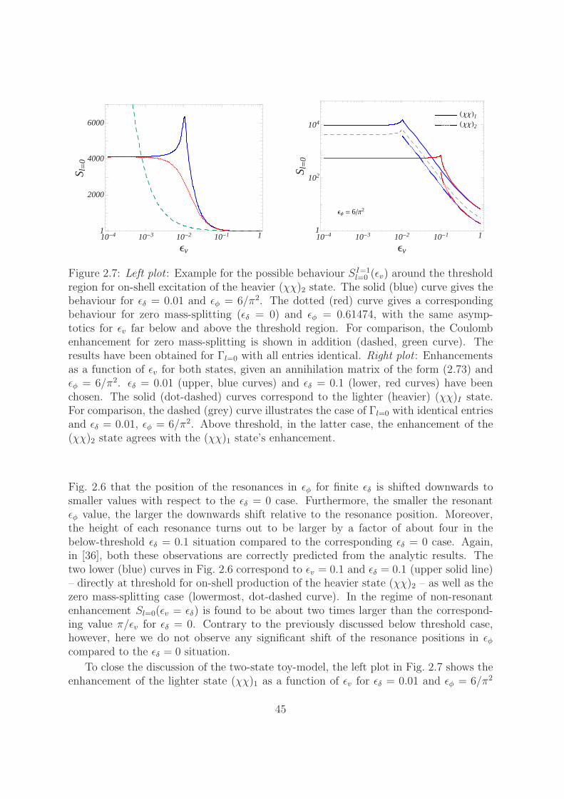
10-4 10-3 10-2 10-1 11
2000
4000
6000
Εv
S l=
0
10-4 10-3 10-2 10-1 11
102
104
Εv
S l=
0
ΕΦ = 6Π2
HΧΧL1HΧΧL2
Figure 2.7: Left plot : Example for the possible behaviour SI=1l=0 (ǫv) around the threshold
region for on-shell excitation of the heavier (χχ)2 state. The solid (blue) curve gives thebehaviour for ǫδ = 0.01 and ǫφ = 6/π2. The dotted (red) curve gives a correspondingbehaviour for zero mass-splitting (ǫδ = 0) and ǫφ = 0.61474, with the same asymp-totics for ǫv far below and above the threshold region. For comparison, the Coulombenhancement for zero mass-splitting is shown in addition (dashed, green curve). Theresults have been obtained for Γl=0 with all entries identical. Right plot : Enhancementsas a function of ǫv for both states, given an annihilation matrix of the form (2.73) andǫφ = 6/π2. ǫδ = 0.01 (upper, blue curves) and ǫδ = 0.1 (lower, red curves) have beenchosen. The solid (dot-dashed) curves correspond to the lighter (heavier) (χχ)I state.For comparison, the dashed (grey) curve illustrates the case of Γl=0 with identical entriesand ǫδ = 0.01, ǫφ = 6/π2. Above threshold, in the latter case, the enhancement of the(χχ)2 state agrees with the (χχ)1 state’s enhancement.
Fig. 2.6 that the position of the resonances in ǫφ for finite ǫδ is shifted downwards tosmaller values with respect to the ǫδ = 0 case. Furthermore, the smaller the resonantǫφ value, the larger the downwards shift relative to the resonance position. Moreover,the height of each resonance turns out to be larger by a factor of about four in thebelow-threshold ǫδ = 0.1 situation compared to the corresponding ǫδ = 0 case. Again,in [36], both these observations are correctly predicted from the analytic results. Thetwo lower (blue) curves in Fig. 2.6 correspond to ǫv = 0.1 and ǫδ = 0.1 (upper solid line)– directly at threshold for on-shell production of the heavier state (χχ)2 – as well as thezero mass-splitting case (lowermost, dot-dashed curve). In the regime of non-resonantenhancement Sl=0(ǫv = ǫδ) is found to be about two times larger than the correspond-ing value π/ǫv for ǫδ = 0. Contrary to the previously discussed below threshold case,however, here we do not observe any significant shift of the resonance positions in ǫφcompared to the ǫδ = 0 situation.
To close the discussion of the two-state toy-model, the left plot in Fig. 2.7 shows theenhancement of the lighter state (χχ)1 as a function of ǫv for ǫδ = 0.01 and ǫφ = 6/π2
45
(≈ 0.607927) (solid, blue curve) and ǫδ = 0, ǫφ = 0.614747 (dotted, red curve). In theǫδ > 0 case, SI=1
l=0 is a non-monotonic function of ǫv, showing a ‘spike’ at threshold foron-shell production of (χχ)2. This behaviour is a threshold effect, which occurs here ontop of resonant enhancement due to a loosely-bound state in the spectrum of the theory.The purely resonant enhancement in the ǫδ = 0 case is illustrated by the dotted (red)curve. The chosen ǫφ values for both curves are slightly different, reflecting the factthat resonance positions are shifted downwards for finite ǫδ values. For comparison andto highlight the fact, that the ǫφ values are associated with resonant enhancement, thedashed (green) curve gives the Coulomb enhancement in the case of zero mass-splitting.As regards the ǫδ > 0 case, the enhancement around threshold is found to be less thantwice as large as the saturated enhancement for ǫv → 0; see [36] for an analytic estimateof this factor. It is argued in [36] that in any case the ratio of S(ǫv = ǫδ)/S(ǫv = 0)should be bounded by two from above.
In the right-hand plot of Fig. 2.7 we show the enhancement factors for both states(χχ)I=1,2 for an annihilation-matrix with non-identical entries of the form (2.73). Al-though the annihilation rate of the heavier state is a factor of four larger than thecorresponding rate of the lighter state, the enhancements of the former state are foundto be a factor of about four smaller compared to (χχ)1. For comparison, the enhance-ment for an annihilation matrix with all entries identical and fixing ǫδ = 0.01, ǫφ = 6/π2
is shown in addition (dashed, grey curve). In the latter case, SI=1l=0 (ǫv) is found to agree
with SI=2l=0 (ǫv) above threshold.
46

Chapter 3
Relic abundance calculation
In this chapter we present the formalism needed for the determination of the relic abun-dance of a weakly interacting massive particle χ1. We start with a brief qualitativediscussion of the phenomenon of freeze-out of the χ1’s annihilation reactions in courseof the Universe’s expansion in Sec. 3.1. The description is subsequently quantified byintroducing an (integrated) form of the Boltzmann equation, appropriate to describe theevolution of particle number densities in the expanding Universe. In Sec. 3.2 the settingis generalised to include the case of co-annihilations of several nearly mass degeneratespecies χi, i=1,...,N . In addition a convenient form of the Boltzmann equation is derivedthat treats the decrease of the number densities due to the expansion of the Universeimplicitly. A single-integral formula for the thermally averaged annihilation rate 〈σeff v〉that enters the Boltzmann equation as central ingredient is finally given in Sec. 3.3.The formula involves the individual annihilation rates σijv of all co-annihilating pairsχiχj . In Chapters 6 – 8 we determine explicit expressions for the rates σijv in χ0/χ±
co-annihilations including Sommerfeld enhancements. On the one hand this chapter istherefore a self-contained short review of the dark matter relic abundance calculation.On the other hand all necessary formulae are provided that allow a direct calculation ofthe χ0
1 relic abundance including Sommerfeld enhancements, provided the (Sommerfeld-enhanced) rates σijv are known.
3.1 The Boltzmann equation
The standard explanation for the origin of a particle species in our present Universestarts from the assumption of its thermal production in the very early Universe. Thisimplies that in these early times the species should have been in both chemical andkinetic equilibrium with the further particle constituents of the early Universe’s thermalplasma. Such equilibrium state requires rapid annihilation and creation processes ofthe particle species as well as effective scattering reactions with the further particlespresent. Note that in general, in this picture, the early Universe’s thermal plasma isassumed to be constituted by the particle species of the Standard Model as well aspossibly additional species occurring in extensions of the SM. The expansion of the
47

Universe, which can conveniently be associate with the expansion rate given by theHubble parameter H (H(t) = d
dtR(t)/R(t), where R(t) denotes the scale factor as a
function of time), runs contrary to the processes that allow the maintenance of thermalequilibrium: it dilutes the actual number densities of the species. As a consequenceinteraction processes will become rare, finally leading to the fact that – depending on thestrength of the interaction rates – a certain species will no longer stay in equilibrium withthe others. Its annihilation and creation reactions stop more or less suddenly (“freezeout”) such that its particle number eventually stays constant (“freezes in”), giving riseto the thermal relic abundance observable today.1 As a very rough criterion this happenswhen the Universe’s expansion rate H starts to dominate over the total annihilation rateΓ of the species, H >∼Γ. Depending on the average thermal velocity of the species duringfreeze-out, non-relativistic (v ≪ 1) or (semi-)relativistic (v . 1), one distinguishes coldor warm/hot thermal dark matter. The neutralino dark matter candidate χ0
1 that weconsider in this work is a cold thermal dark matter candidate; its freeze-out should haveoccurred for thermal bath temperatures around T ∼ mχ0
1/20. Therefore we focus here
on the case of heavy cold dark matter candidates.
The first quantitative studies of the freeze-out process of a heavy particle speciesfocused on a possible heavy neutrino relic. They were performed in the late 1970s byLee and Weinberg [44] as well as independently by other authors and led to a lowerbound on the mass of a heavy neutrino species, today referred to as the “Lee-Weinbergbound”. Since that time the theoretical description, relying on Boltzmann equationsfor the particle number densities in the expanding Universe, has been subsequently re-fined. Both improved analytical approximations and numerical solution methods havebeen applied [45–47] and a consistent treatment of co-annihilations in the (roughly) si-multaneous freeze-out process of several (nearly) mass-degenerate heavy species has beengiven [48]. In addition the case of resonant annihilation reactions has been addressed [48]and the annihilation rates entering the Boltzmann equations of the non-relativistic par-ticles can be consistently calculated including relativistic corrections, beyond the strictnon-relativistic approximation [49]. Regarding the solution of the Boltzmann equationand the necessary input related to the thermodynamics in the expanding Universe, thedetermination of the thermal relic abundance of a particle species, which represents aviable dark matter candidate, has become a standard calculation. It is implementedin several computer codes, such as DarkSUSY [5] and micrOMEGAS [6]. The dominantuncertainties in the determination of the final abundance are currently associated withthe annihilation rates entering the Boltzmann equations. These rates are an input fromthe particle physics model that provides the respective particle dark matter candidate.While the publicly available codes currently rely on tree-level annihilation rates, we aim
1In the Universe today annihilation reactions of a species that underwent freeze-out in earlier timescan start again. This may happen if due to gravitational attraction regions with a high number densityof the particular species have formed, such as for example in the halo of galaxies, in galactic centres orpossibly also in the Sun. If the particle dark matter hypothesis is true, dark matter pair-annihilationreactions should occur in these regions, giving rise to indirect detection signals in terms of cosmic raysor gamma ray lines. For an introduction to indirect dark matter searches see for example [3, 4].
48
to study the impact of Sommerfeld-enhanced cross sections on the predicted relic abun-dance. To this end we have developed a code that allows for the determination of the χ0
1
dark matter relic abundance including Sommerfeld enhancements. We come back to thecalculation of the rates in later chapters and proceed in this section with the derivationof the relevant generic formulae needed in the relic abundance determination. Our fol-lowing discussion is mainly based on the textbook [50] as well as on the articles [3] andthe more recent [4], which provide a nice review of the freeze-out of weakly interactingmassive particles.
The Boltzmann equation describes the evolution of the phase space distributionf(pµ, xµ) of a particle species and can be expressed as
L[f(pµ, xµ)] = C[f(pµ, xµ)] . (3.1)
Let us in particular refer to the distribution function and corresponding Boltzmann equa-tion of particle species χ1 in the following. In the expanding Universe the left-hand side of(3.1) contains the covariant relativistic form of the Liouville operator acting on f(pµ, xµ).The right-hand side is the collision term associated with all particle scatterings as wellas annihilation or creation reactions, that change the distribution function f(pµ, xµ) ofspecies χ1. Under the assumption of a homogeneous and isotropic Universe described bythe Friedman-Robertson-Walker metric, any phase space distribution function dependsonly on time and energy, f(E = p0, t), and the Liouville operator becomes
L[f(E, t)] = E∂
∂tf(E, t) − H(t) ~p 2 ∂
∂Ef(E, t) . (3.2)
H(t) denotes the Hubble parameter. Instead of f(E, t), we will be interested in theevolution of the particle number density
n(t) = g
∫d3~p
(2π)3f(E, t) , (3.3)
with g the particle’s internal (spin) degree of freedom. Dividing the Boltzmann equationby E and integrating over the three-momentum finally leads to the integral form
dn
dt+ 3H(t)n = g
∫d3~p
(2π)31
EC[f(E, t)] . (3.4)
After the momentum integration only those contributions to the collision term survivethat change the actual number of χ1 particles. These are related to annihilation andcreation reactions involving species χ1. As in general 2 → 2 reactions will be mostimportant in the thermal plasma, the relevant annihilation and creation processes aregiven by χ1χ1 → XAXB and XAXB → χ1χ1 reactions. XA, XB denote any other particlespecies present in the thermal bath that undergo interactions with species χ1. Here wehave implicitly assumed that the χ1 is its own anti-particle, such that the only 2 → 2reactions changing the number of χ1s present in the thermal bath are χ1χ1 ↔ XAXB
49
processes (provided that the χ1 is stable or at least sufficiently long-lived and interactionsχ1χi ↔ XAXB with other species χi changing the χ1 number are irrelevant). This appliesif the χ1 is a real scalar or Majorana fermion, while in case of a charged scalar or Diracfermion, χ1χ1 ↔ XAXB processes involving the anti-particle χ1 have to be considered.There is one subtle point in the former case, which is related to symmetry factors and thenumber of χ1s created or annihilated per χ1χ1 ↔ XAXB reaction. In each χ1χ1 ↔ XAXB
process the number of χ1s is changed by two, such that one might expect a factor of 2 infront of the collision term on the right-hand side of (3.4). However, in the collision term asymmetry factor of 1/2 has to be taken into account when the momentum integration overthe two identical particles in the (initial or final) χ1χ1 state is performed, such that thesetwo factors, both related to identical particle states, eventually cancel each other out. Inthe following we take the cancellation of these two factors for granted and therefore writeneither of the two explicitly. Note that although (elastic) scattering χ1XA → χ1XB withthe thermal bath constituents XA,B (assumed to be in thermal equilibrium during χ1
freeze-out) does not contribute to the momentum integrated right-hand side in (3.4), itplays an important role in maintaining species χ1 in kinetic equilibrium2 even after itis chemically decoupled from the thermal plasma [45]. We come back to this importantfeature later in this chapter. Altogether, the reactions χ1χ1 ↔ XAXB determine thecollision term in the following way:
g
∫d3~p
(2π)31
EC[f(E, t)]
⊃ −∑
spins
∫d3~p
2E(2π)3d3~p ′
2E ′(2π)3d3~pA
2EA(2π)3d3~pB
2EB(2π)3× (2π)4 δ(4)(p+ p′ − pA − pB)
×(f(E, t)f(E ′, t) |Aχ1χ1→XAXB
|2 − fA(EA, t)fB(EB, t) |AXAXB→χ1χ1|2). (3.5)
A rigorous derivation of this expression3 can be addressed within thermal field theory.From heuristic arguments the origin of the different terms is however clear: the squaredamplitudes |Aχ1χ1→XAXB
|2 and |AXAXB→χ1χ1|2 describe the quantum mechanical transi-
tion probabilities of reactions χ1χ1 → XAXB and XAXB → χ1χ1 and generically dependon the four-momenta of the four particles taking place in the scattering reaction. Toobtain the transition rates, a phase space integration of the final state particles hasto be performed and a summation over the spins of all involved particles has to becarried out. Subsequently each of these transition rates is weighted by the product ofthe incoming particles’ statistical distributions (f(E, t)f(E ′, t) ≡ fχ1
(E, t)fχ1(E ′, t) or
fA(EA, t)fB(EB, t)) and finally integrated over the initial state momenta.
2We assume the presence of such interactions, keeping the χ1 close to kinetic equilibrium, through-out. Several authors have studied the effect of kinetic decoupling of the χ1 that occurs after chemicaldecoupling if χ1XA → χ1XB reactions cease to maintain species χ1 in kinetic equilibrium, see forexample [40, 51, 52].
3Note that we have already dropped Fermi blocking and Bose stimulated emission factors in (3.5)(for a corresponding discussion see for example [50]).
50
To proceed let us assume that apart from χ1 all thermal bath species X are inthermal equilibrium throughout the time within which we track the evolution of theχ1 number density. Consequently the phase space distribution fX(E, t) of such speciesin the cosmic comoving frame, where the plasma is at rest as a whole, is given by thethermal equilibrium distribution
fX, eq(E, t) =1
exp(E/T ) + ηX, (3.6)
where ηX is 1 (−1) if X is of fermionic (bosonic) nature. Note that we have dropped thechemical potential µX of species X . This is in general a good approximation for the earlyUniverse, as the chemical potential µX is generically much smaller than the energies Eat the temperatures of interest to us: Energies in on-shell reactions χ1χ1 ↔ XAXB ofnon-relativistic χ1 particles will be characterised by the scale 2mχ1
(up to correctionsof the order of the non-relativistic kinetic energy), which for a heavy cold dark mattercandidate is at least of the order of some hundred GeV to some TeV. Further, in the χ1
freeze-out process only temperatures T . mχ1/20 are relevant. In this case the exact
expression (3.6) can be replaced in very good approximation by a Maxwell-Boltzmanndistribution, fX, eq(E, t) ≃ e−E/T , such that from energy conservation, E+E ′ = EA+EB,the relation
fA, eq(EA, t) fB, eq(EB, t) = feq(E, t) feq(E′, t) (3.7)
is obtained. The phase space integration related to the species XA and XB in (3.5)can now be performed independently of fA and fB. With the definition of the Lorentzinvariant cross section we arrive at the relation
∑
spins
∫d3~pA
2EA(2π)3d3~pB
2EB(2π)3× (2π)4 δ(4)(p+ p′ − pA − pB) |Aχ1χ1→XAXB
|2
= 4 g g′√
(p · p′)2 −m2χ1m2χ1
σχ1χ1→XAXB. (3.8)
g, g′ denote the spin factors (internal degrees of freedom) of the two χ1 initial state par-ticles. As first argued in [49], unitarity ensures that when replacing |Aχ1χ1→XAXB
|2 inthe integrand on the left-hand side by |AXAXB→χ1χ1
|2, the same right-hand side expres-sion as in (3.8) results. Summing over all possible states XAXB, the collision term thensimplifies to
g
∫d3~p
(2π)31
EC[f(E, t)] =
−g∫
d3~p
(2π)3g′∫
d3~p ′
(2π)3
[f(E, t)f(E ′, t) − feq(E, t)feq(E
′, t)]× (σχ1χ1
v) . (3.9)
σχ1χ1≡ σχ1χ1→
∑XAXB
denotes the total annihilation cross section for χ1χ1 pair annihi-lations and v is the Møller velocity defined as [49]
v =
√(p · p′)2 −m4
χ1
E E ′ . (3.10)
51
Note that the Møller velocity v coincides with the relative velocity vrel for anti-collinearcollisions ~p ′ ∝ ~p.
In the next step, the distribution functions f(E, t) and f(E ′, t) in (3.9) are approx-imated by a momentum independent factor times the (chemical and kinetical) ther-mal equilibrium Maxwell-Boltzmann distribution, that is f(E, t) = α(t)feq(E, t) withfeq(E, t) = e−E/T . The proportionality factor α(t) may depend (through its time de-pendence) on the temperature of the thermal bath, but is independent of the particle’senergy. As argued in [45], this approximation holds if two conditions are fulfilled. First,the temperature of the thermal bath is already well below the mass scale of the speciesχ1, T ≪ mχ1
, such that the Maxwell-Boltzmann distribution gives a good approxima-tion to the equilibrium distribution. Second, scattering reactions χ1XA → χ1XB withthe thermal plasma constituents XA,B have to be rapid and effective enough to main-tain species χ1 in kinetic equilibrium. In this case the momentum dependence of thedistribution function stays close to its equilibrium functional dependence and the pro-portionality factor α(t) is momentum independent in very good approximation, see thecorresponding discussion in [45]. Under these assumptions, (3.9) can finally be cast inthe form
g
∫d3~p
(2π)31
EC[f(E, t)] = −〈σ v〉 (n2 − n2
eq) , (3.11)
with the thermally averaged total annihilation cross section
〈σ v〉 =1
n2eq
g
∫d3~p
(2π)3g′∫
d3~p′
(2π)3(σχ1χ1
v) feq(E, t) feq(E′, t) . (3.12)
neq denotes the equilibrium number density obtained from the Maxwell-Boltzmann dis-tribution feq(E, t) using (3.3). Finally, from (3.4) and (3.11), the familiar expression forthe Boltzmann equation in the expanding Universe
d
dtn = 3H(t)n − 〈σχ1χ1
v〉(n2 − n2
eq
)(3.13)
is obtained. The first term on the right-hand side accounts for the dilution of the numberdensity due to the Universe’s expansion and the second term accounts for the particlephysics processes that change the number of particles χ1.
3.2 Co-annihilations
In Sec. 3.1 we discussed the single χ1 species freeze-out process, which is quantifiedby the evolution of the χ1 number density governed by a Boltzmann equation. In thederivation of the central equation (3.13) it is implicitly assumed, that the remainingconstituents of the thermal bath (generically denoted with XA,B) are in chemical andkinetical equilibrium at least until the χ1 annihilation reactions are completely frozenout. However, this does not apply if in addition to the χ1 there are further slightly
52
heavier species χi, i > 1, present, that have comparable interaction strength and interactwith the χ1. Being only slightly heavier, the species χi will be roughly as abundantas the χ1 as long as chemical equilibrium holds.4 Given interaction rates of similarstrength, the freeze-out of species χi and χ1 will take place around the same time. Inparticular the evolution of the number densities ni will affect the n1 evolution due tocoupled Boltzmann equations. This effect of co-annihilations has first been addressedin [48], where a consistent formalism to treat co-annihilations in the relic abundancecalculation of species χ1 has been given, applicable to the limit of strictly non-relativisticco-annihilation rates. Using the exact relativistic formulae for the annihilation rates inthe single species freeze-out from [49], [53] subsequently provided a formalism that allowsto include exact co-annihilation rates in dark matter relic abundance calculations, whichin [53] was applied to the χ0
1 relic abundance calculation in the MSSM.Our application in Chap. 9 is the relic density calculation of O(TeV) scale χ0
1 darkmatter in the MSSM. In this case co-annihilation processes with further neutralino andchargino species occur generically. A TeV-scale χ0
1 that reproduces the observed cold darkmatter as thermal relic has to be either wino- or higgsino-like, or a mixed wino-higgsinostate. In these cases mass degeneracies between the χ0
1 and at least its correspondingchargino partner χ±
1 at O(GeV) or below are generic, making the consideration of co-annihilations in the relic abundance calculation necessary.5 Following [48,53] we thereforegeneralise the derivation from Sec. 3.1 here to include the effect of co-annihilations.
Consider a set of N nearly mass degenerate species χi, i = 1, . . . N, ordered accordingto their increasing masses mi (mj ≤ mk for j < k). The lightest species χ1 is the darkmatter candidate. Further the existence of a conserved multiplicative quantum number isassumed, in which all species χi shall differ from the SM particles. The latter guaranteesthe stability of the dark matter candidate χ1. Within the R-parity conserving MSSMconsidered in Chap. 9 R-parity takes exactly the role of this additional multiplicativequantum number. In the following XA,B denote SM particle species and it is assumedthat these species are in chemical equilibrium throughout the freeze-out of co-annihilationreactions of the χi. The following processes can then change the number of species χi:
χi χj ↔ XA XB , (3.14)
χi XA ↔ χj XA , (3.15)
χi ↔ χj XA XB , j < i . (3.16)
Decay processes (3.16) imply that all species χi>1 will eventually decay into the lightest
4Generically at temperature T , the equilibrium number density ni, eq of a heavier species χi willbe suppressed relative to the density n1, eq of the (non-relativistic) species χ1 by a Boltzmann factore−(mi−m1)/T , where mi (m1) is the mass of species χi (χ1). See the end of Sec. 3.3 for a discussion onthe origin of such Boltzmann suppression factor. For small mass splittings δmi = mi − m1 ≪ T thenumber densities ni, eq and n1, eq are therefore of the same order.
5In addition to the rather natural mass degeneracies in the χ0/χ± sector for TeV-scale χ01 dark matter
scenarios, there are viable χ01 dark matter models where co-annihilations with nearly mass-degenerate
third generation sfermions (the t1 or τ1) allow to reproduce the experimentally observed dark matterdensity. We focus here on χ0/χ± co-annihilations and exclude the case of additional mass degeneraciesof the χ0
1 with sfermion or Higgs states in the MSSM from our analysis.
53
and stable χ1, such that the number density of the latter today is determined from thesum over the number densities ni of all χi species, n =
∑i=1,...N ni. While annihilation
and creation reactions (3.14) affect the total number density n of all χi species, thedecay and inverse decay processes (3.16) cannot change n. Finally scattering reactions(3.15) affect neither n nor ni, but are important to keep the individual χi close to kineticequilibrium even after the species have chemically decoupled. With these preliminariesthe Boltzmann equation corresponding to (3.13), that describes the evolution of thesummed number density n =
∑i=1,...N ni, takes the form
d
dtn = −3H(t)n −
∑
i,j
〈σχiχjvij〉 (ni nj − ni, eq nj, eq) . (3.17)
The χiχj annihilation cross section σχiχjis defined by an obvious generalisation of (3.8)
and similarly the Lorentz-invariant Møller velocity vij derives from (3.10),
vij =
√(pi · pj)2 −m2
χim2χj
EiEj. (3.18)
Note that the sum in (3.17) separately runs over i, j = 1, . . . N . Under the assumptionof rapid scattering reactions (3.15) with the SM thermal plasma it is argued in [53] thatthese processes ensure, that the ratio of particle number density ni to the total particlenumber density n remains close to the corresponding ratio of equilibrium quantities,
nin≃ ni, eq
neq
. (3.19)
This allows the following rewriting of the Boltzmann equation:
d
dtn = −3H(t)n − 〈σeff v〉
(n2 − n2
eq
), (3.20)
with the thermally averaged effective annihilation cross section
〈σeff v〉 =∑
i,j
〈σχiχjvij〉
ni, eq nj, eqn2eq
. (3.21)
(3.20) is the generalisation of (3.13) that properly includes co-annihilations. Instead ofn it is more convenient to consider the evolution of the yield Y ,
Y =n
s, (3.22)
where s denotes the total entropy density, as this allows to tread the dilution effect fromthe Universe’s expansion implicitly. Assuming the absence of entropy production, thetotal entropy per comoving volume element, S = sR3, remains constant and the change
54
of number and entropy density due to the expansion is the same, namely ds/dt = −3Hs.From (3.20) we then obtain the Boltzmann equation for the yield,
d
dtY = −s〈σeff v〉
(Y 2 − Y 2
eq
). (3.23)
Instead of its time evolution it is more useful to consider the change of Y with thetemperature T of the Universe’s thermal bath. This temperature is associated withthe bath of thermal photons in the Universe throughout its evolution. In particular,introducing the dimensionless inverse scaled temperature x = mχ1
/T and noting that inabsence of entropy production
dx
dt=
x2
mχ1
3H sdT
ds(3.24)
we obtain
d
dxY = − mχ1
3H x2ds
dT〈σeff v〉
(Y 2 − Y 2
eq
). (3.25)
In order to determine the change of the entropy density with the thermal bath temper-ature, ds/dT , consider the Friedmann equation
H2 =8πGN
3ρ , (3.26)
where GN is the gravitational constant. Freeze-out of the heavy species χi will takeplace during the radiation-dominated epoch, such that the energy density ρ on the right-hand side is dominated by relativistic degrees of freedom. It is therefore convenient toparametrise the total energy density ρ as well as the total entropy density s by
ρ =π2
30geff(T ) T
4 , s =2 π2
45heff(T ) T
3 . (3.27)
geff and heff denote the effective degrees of freedom associated with the energy and entropydensity in the thermal bath [49]. From (3.27) the change of s with T is obtained.(3.26) together with the parametrisation of ρ in (3.27) finally allows to relate the Hubbleparameter H to the thermal bath temperature, such that the Boltzmann equation canbe rewritten to
d
dxY = −
√π
45GNg1/2∗
mχ1
x2〈σeff v〉
(Y 2 − Y 2
eq
)
= − 2√10πmPl
15g1/2∗
mχ1
x2〈σeff v〉
(Y 2 − Y 2
eq
). (3.28)
In the last step we have introduced the reduced Planck mass mPl related to GN viamPl = (8πGN)
−1/2, with the numeric value mPl = 2.42888 · 1018GeV. The temperature
dependent parameter g1/2∗ in (3.28) is defined as
g1/2∗ =heff√geff
(1 +
T
3 heff
d
dTheff
). (3.29)
55
Under the three assumptions that first essentially only the SM species contribute to heffand geff at temperatures of interest,6 that second all these species behave as an ideal gasand that third no entropy is produced, simple analytic approximations to heff and geff canbe given, see [49]. In a more accurate treatment the QCD quark-hadron phase transition
has to be taken into account [54]. The numerical results for heff, geff and hence g1/2∗
from such more involved calculations are tabulated and publicly available (for examplethey are provided with the codes DarkSUSY [5] and micrOMEGAS [6]). When numericallysolving the Boltzmann equation to determine the χ0
1 relic abundance in some popular
MSSM scenarios in Chap. 9, we access these tabulated values of heff, geff and g1/2∗ . The
equilibrium yield in (3.28) is given by
Yeq =45
4 π4
x2
heff
∑
i
gimi
mχ1
K2
(xmi
mχ1
), (3.30)
with K2 the modified Bessel function of the second kind of order 2, and is obtainedupon integration of equilibrium Maxwell-Boltzmann distributions for the species χi anddivision by the total entropy density s in (3.27).
The Boltzmann equation (3.28) is the central expression in this section. For tem-peratures x . 1 (T >∼mχ1
) all species χi should still have been in chemical equilibriumwith the plasma, which provides the boundary condition Y (x = 1) = Yeq(x = 1) for thenumerical integration of (3.28). To determine the yield Y0 associated with the numberdensity of the stable species χ1 today, the integration has to be carried out starting fromx = 1 to today, x0 = mχ1
/T0 ∼ O(1010) (given a TeV scale species χ1 and temperatureT0 = 2.725K = 2.34823 · 10−13GeV of the photon background radiation today). As wewill see in Chap. 9, a value x0 ∼ 108 is typically sufficient for practical purposes in thenumerical solution. From Y0 the relic abundance is finally obtained as
Ωχ1h2 =
ρχ1
ρcrh2 =
mχ1s0Y0ρcr
h2 . (3.31)
s0 denotes the entropy density today and can be determined from (3.27). The corre-sponding heff(T0) is essentially given by the photon and neutrino degrees of freedom,associated with the photon and neutrino background radiation today, heff(T0) = 3.9139.The critical energy density ρcr is given by ρcr = 3H0/8πGN where H0 denotes the Hubbleparameter today. It takes the numerical value ρcr = 1.05368× 10⁻⁵ h2GeVcm−3.
3.3 Thermally averaged annihilation cross sections
In order to finally solve the Boltzmann equation (3.28), an explicit expression of thethermally averaged effective annihilation rate 〈σeff v〉 defined in (3.21) is needed. In [49],where the case of one particle species χ1 was considered, a single-integral formula for
6For the relic abundance calculation of a dark matter candidate with a freeze-out temperature ofsome 10− 100GeV, this is certainly fulfilled.
56
〈σeff v〉 in terms of Lorentz invariant quantities was derived. Subsequently the expressionwas generalised to include co-annihilations in [53]. The starting point in the derivationof the single-integral formula for 〈σeff v〉 is the defining equation (3.21), with the thermalaverages 〈σijvij〉 of the individual rates performed in the cosmic comoving frame wherethe plasma is at rest as a whole. In this case the phase space distribution functionsfi, eq that enter the thermally averaged rates 〈σijvij〉 and number densities ni, eq aregiven by Bose-Einstein or Fermi-Dirac distributions (3.6). As already used in Sec. 3.1and 3.2, both distributions are well approximated by Maxwell-Boltzmann distributionsfi, eq = e−Ei/T for temperatures T ≤ mχ1
/20, that are relevant in the co-annihilating χisfreeze-out. Starting from (3.21) we can therefore write
〈σeff v〉 =1
n2eq
∑
i,j
gi gj
∫d3~pi(2π)3
∫d3~pj(2π)3
σijvij e−(Ei+Ej)/T , (3.32)
with the total equilibrium number density of the co-annihilating species χi=1,...,N given
by neq =∑N
i=1 ni, eq, and
ni, eq = gi
∫d3~pi(2π)3
e−Ei/T =T
2π2gi m
2i K2(mi/T ) . (3.33)
gi denotes the internal degrees of freedom of species χi. Note that the individual particleenergies Ei, Ej in (3.32) explicitly refer to the cosmic comoving frame, while the crosssections σij and the Møller velocities vij by definition are Lorentz invariant quantities.After a convenient change of variables following [49, 53], (3.32) can be simplified to thesum of single-integral expressions
〈σeff v〉 =1
n2eq
∑
i,j
gi gj8π4
T
∫ ∞
(mi+mj)2ds√s p2ij σij K1(
√s/T ) , (3.34)
with K1 the modified Bessel function of the second kind of order 1. The integrationvariable s is the Lorentz-invariant centre-of-mass energy s = (pi + pj)
2 in the individualχiχj pair-annihilation reaction, where pi,j denote the 4-momenta of the annihilatingparticles. Finally, pij is the modulus of the individual particles’ momenta in the centre-of-mass frame of the χiχj annihilation reaction. Expressed in terms of Lorentz invariantquantities it reads
pij =
√(pi · pj)2 −m2
i m2j
s=
1√s
√s2
4− s
2(m2
i +m2j ) +
(m2i −m2
j )2
4. (3.35)
While [53] now proceeds by interchanging summation and integration in (3.34) and in-troduces an effective rate given by the sum over the individual integrands related tothe pairs χiχj , we follow a slightly different way and consider each integral in (3.34)separately. In Chap. 6 and 8 we determine the product σij vrel ≡ σij vrel, ij of the anni-hilation cross section σij times the relative velocity vrel, ij in the centre-of-mass frame of
57
the annihilation reaction, rather than the separate cross sections σij . The centre-of-massframe relative velocity of the χiχj pair expressed in terms of Lorentz invariant quantitiesis given by
vrel, ij = pij√s
4s
s2 − (m2i −m2
j)2. (3.36)
Note that vrel, ij coincides with the Møller velocity vij in any frame where the two particlesχi, χj move collinearly. Our final result for the thermally averaged effective annihilationcross section that enters the Boltzmann equation (3.28) and involves the individual ratesσijvrel therefore reads
〈σeff v〉 =
1
n2eq
∑
i,j
gi gj8π4
T
∫ ∞
(mi+mj)2ds pij (σij vrel)
s2 − (m2i −m2
j )2
4sK1(√s/T ) . (3.37)
In application of the presented formalism to the χ01 relic abundance calculation in the
MSSM in Sec. 9 we generically take all co-annihilating neutralino and chargino speciesin 〈σeff v〉 into account. Note however that the contribution from a heavy channelχiχj is typically suppressed by a factor proportional to e−(mi+mj−2m1)/T with respectto the contribution from the lightest state χ1χ1. This (Boltzmann) suppression arisesfrom the asymptotic expansion of the Bessel function K1 in the integrand for large√s/T ≫ 2m1/T ≫ 1 for temperatures T ≤ m1/20 relevant in the cold dark matter
relic abundance calculation. We determine all neutralino/chargino co-annihilation ratesσij vrel entering (3.37) in a non-relativistic (partial-wave) expansion, including O(v2rel) cor-rections to the hard annihilation reactions in Chap. 6. The effect of Sommerfeld-enhancedco-annihilation rates on the calculated χ0
1 relic abundance is the particular phenomeno-logical focus of this thesis. Consequently Sommerfeld enhancements on the hard ratesof all those χiχj pairs that can be produced on-shell from reactions χ1χ1 → χiχj ofnon-relativistic χ1χ1 states are included in the calculation of 〈σeff v〉 in our final analysesin Chap. 9. Before we can enter the detailed study of some popular MSSM benchmarkmodels we introduce the framework needed for the calculation of Sommerfeld-enhancedrates σijvrel in the next chapters. We finally come back to the relic abundance calculationand apply the formulae derived here in Chap. 9.
58
Chapter 4
The neutralino and chargino sectorin the MSSM
In this chapter we discuss the neutralino and chargino sector of the MSSM – in particularthe corresponding mass spectrum – in view of its properties relevant to our investigationof Sommerfeld enhancements and the neutralino relic abundance calculation. Howeverbefore focusing on this subject we prepend in Sec. 4.1 a short discussion on problems ofthe Standard Model of particle physics, followed by a basic introduction to supersym-metry that possibly may help to solve or to change for better the aforementioned issues.Subsequently an overview on the field content and parameters in the general MSSM isgiven in Sec. 4.2. With the background of the preceding sections we finally concentrate inSec. 4.3 on the neutralino and chargino sector of the MSSM. We conclude in Sec. 4.4 withsome remarks on the generation of MSSM spectra to be analysed in view of Sommerfeldenhancement effects in neutralino and chargino co-annihilations in Chap. 9, emphasisingthe fact that a sound analysis requires the knowledge of the neutralino and charginomasses and mixing matrices from on-shell renormalisation at one-loop level.
4.1 Motivations for supersymmetry and basic ideas
The Standard Model of particle physics provides the successful theoretical frameworkto describe elementary interactions of the microscopic constituents associated with ‘or-dinary’ matter – the six quark species, six lepton species, eight gluons, the electroweakgauge bosonsW± and Z, the photon and the Standard Model Higgs boson – up to energyscales currently testable at experiments [1].1 The largest such energy scale reached atpresent is the scale of maximally 8TeV centre-of-mass energy in pp-collisions during thefirst run of the Large Hadron Collider (LHC) at CERN. In 2012 the collaborations AT-LAS and CMS running the two multi-purpose detectors at the LHC had announced thediscovery of a spin-0 particle with the properties of the long sought-after Higgs boson,
1We use the term ‘ordinary’ matter to distinguish it from the Universe’s cold dark matter component,whose elementary constituent (or constituents) – if dark matter has particle nature – is unknown.
59

the last of the particle constituents of the Standard Model that had not been observedexperimentally before.2 Further, no significant deviation of observed particle productionrates from the SM prediction has so far been found at the colliders running at the highenergy frontier.3
In spite of these successful tests the Standard Model is incomplete as it does not in-clude gravitational interactions and is therefore considered to be the low energy effectivetheory of a more fundamental theory of nature that governs the physics at the Planckscale, where gravitational effects eventually become relevant. Several other problems re-lated to both experimental observations and theoretical aspects of the Standard Modelsuggest or directly imply that the Standard Model cannot be the fundamental theoryof microscopic interactions. For instance it is observed experimentally that contrary tothe description in the Standard Model the three neutrino species are not massless butmust have masses in the range of some eV. Similarly, the measurement of the anoma-lous magnetic moment of the muon does not match the Standard Model prediction. Inaddition there also are more formal issues that require an appropriate extension of thetheory. The probably most important ones are the so called ‘hierarchy problem’ andthe non-unification of running SM gauge couplings within the theory. Another severeproblem is the lack of a dark matter particle candidate. We briefly sketch the latterthree issues in the following.
The hierarchy problem is associated with the nowadays widely believed ansatz thatthe Standard Model is an effective theory, which is valid up to a certain energy scalewhere new physics effects will arise. This scale does not have to coincide with theO(1019)GeV Planck scale but can lie in the energy range in between the electroweakscale at O(102)GeV (typically associated with the Higgs field vacuum expectation valuev ≈ 246GeV) and the Planck scale. The hierarchy problem can be formulated as thequestion how to obtain a scale v that is much smaller than the high energy scale denotingthe range of validity of the effective theory. In the perturbative renormalisation of the SMHiggs mass, quantum corrections arise that are quadratic in the cut-off of the effectivetheory. To obtain the experimentally measured value of the Higgs boson mass mH =125.7 ± 0.4GeV [1] a sufficiently fine-tuned cancellation between the bare Higgs massparameter and the quantum corrections has to take place. The hierarchy problem heremanifests itself as a “fine-tuning” or naturalness problem, as the bare mass parameterof the Higgs field and the quantum corrections have to cancel each other over severalorders of magnitude to give the experimentally measured O(102)GeV Higgs mass.
Relying on corresponding renormalisation group equations in the Standard Modelit is found that the scale dependent Standard Model gauge couplings almost (but not
2The spin of the discovered particle, its CP properties and the signal strength in experimentallyobserved decay channels are so far consistent with an interpretation of the new state in terms of aStandard Model Higgs boson, see the corresponding section in [1] and references therein.
3Until 2011 the pp-collider Tevatron at Fermilab was running at maximally 1.96TeV centre-of-massenergy. The LHC at CERN reached maximally 8TeV centre-of-mass energy in run I while in run II,scheduled for 2015, it shall operate at 14TeV centre-of-mass energy. Data from the second LHC runwill hopefully allow to get a deeper insights into the mechanism of electroweak symmetry breaking andthe role that the discovered Higgs boson plays in this context.
60
exactly) meet at some high energy scale between 1012GeV to 1018GeV. This couldbe a hint that the Standard Model gauge group is actually embedded into a largergauge group, for instance SU(5), with only one coupling constant [55]. The largergauge group is associated with the so called grand unification scale, below which it isspontaneously broken to the Standard Model gauge group SU(3)C × SU(2)L × U(1)Y .Above the grand unification scale the symmetry associated with the larger gauge group ishowever restored. The effects of the new physics that become relevant close to the grandunification scale modify the running of the Standard Model gauge couplings such thatan exact unification of these couplings can take place, thus the notion grand unificationof gauge couplings.
We have noted before that various observations exist which imply the existence of acold dark matter component in the Universe. They range from the scale of galaxies togalaxy clusters, large scale structures and finally the largest observable scales associatedwith the cosmic microwave background radiation. While the nature and origin of theobserved dark matter component can be rather naturally explained in terms of a thermalrelic as discussed in Chap. 3, the Standard Model does not provide a suitable particlecandidate. The fact that the calculated thermal relic density of a weakly interactingmassive particle with O(1 TeV) mass and weak interaction strength matches the orderof magnitude of the observed cold dark matter abundance seems to indicate that newphysics, which addresses not only the problem of a missing dark matter candidate butpotentially also further problems of the Standard Model, could be related to the TeVscale.
Several theories have been proposed that solve or amend the problems encounteredin the Standard Model. Probably one of the best motivated and certainly most studiedideas is the concept of a supersymmetric extension of the Standard Model [1, 56–59].Supersymmetry (SUSY) generalises the concept of symmetries in quantum field theoriesby connecting bosonic and fermionic degrees of freedom. Due to formal aspects it is thusan attractive idea. Supersymmetric transformations are space-time transformations: thePoincare algebra is extended to include fermionic generators. When acting on a particlestate, these fermionic generators transform a bosonic state into a fermionic one, andvice versa, by changing the spin in units of one-half. The full symmetry of a modelis given as direct product of the supersymmetry group and possible inner symmetrygroups. Consequently the states are classified by the irreducible representations of thesupersymmetry algebra, called supermultiplets, and the irreducible representations ofthe possible additional inner symmetries. Each supermultiplet must be characterised bythe same number of bosonic and fermionic degrees of freedom. Further, as supersym-metry transformations commute with the inner symmetries, the bosonic and fermionicconstituents of the supermultiplet have to transform in the same representation withrespect to the inner symmetries. This implies that in a supersymmetric extension of theStandard Model new particles have to be introduced to form appropriate supermultipletstogether with the Standard Model species. As long as supersymmetry is unbroken thesupersymmetric partners of the Standard Model species would be mass-degenerate with
61
the latter.4 As these superpartners have not been observed experimentally supersymme-try must be broken. We comment on possible breaking mechanisms in Sec. 4.2 in contextof the Minimal Supersymmetric Standard Model. Let us note that in minimal supersym-metric extensions of the Standard Model only one fermionic supersymmetry generator isconsidered (N = 1), such that each Standard Model particle gets exactly one supersym-metric partner. In extended supersymmetric models more than one fermionic generatorappears in the supersymmetry algebra (N > 1).
Supersymmetric theories, in particular the mechanism that breaks the mass degenera-cies between the Standard Model particles and their supersymmetric partners, introducenew energy scales that can provide a solution or mitigation to the hierarchy problem. Inparticular, a solution of the fine-tuning problem is possible due to the fact that the newparticles give additional contributions to the radiative corrections to the Higgs mass.Because contributions from a bosonic and a fermionic loop (related to particles withinthe same supermultiplet) come with a relative minus sign, the quadratic divergenciescan compensate each other. Such cancellation however works only as long as the super-partners are not heavier than O(TeV). Otherwise the hierarchy problem is reintroduced.The presence of the superpartners also changes the renormalisation group running of thegauge couplings discussed above, such that a unification of the gauge couplings at somehigh energy scale becomes possible. Finally – and for our purposes most importantly –some of the additional particles in supersymmetric theories that enlarge the number ofparticle species considered in the Standard Model are viable dark matter candidates.
Let us further point out that a supersymmetric model can eventually be extendedto include gravity by promoting to local supersymmetry transformations, where theresulting non-renormalisable theory is called supergravity theory [60].
4.2 The MSSM: field content and parameters
The Minimal Supersymmetric Standard Model is a N = 1 supersymmetric theory basedon the Standard Model gauge group GSM = SU(3)C×SU(2)L×U(1)Y . The field contentof the Standard Model is extended by adding appropriate fermionic and bosonic partnerfields. Several reviews and textbooks on the construction and the properties of theMSSM exist, see for example [1, 56–59] and references therein. In the calculation ofMSSM neutralino and chargino co-annihilation rates in later chapters, we refer to thenotation and conventions established in the two review articles [56] and [61], where thelatter reference focuses on the MSSM Higgs sector. In addition we rely on the set ofMSSM Feynman rules collected in [62]. All the three latter references use the sameconventions. The following brief summary on the MSSM field content is based on [62].
4The operator P 2, square of the 4-momentum operator Pµ that appears as one of the bosonicgenerators in the supersymmetry algebra, is a Casimir operator of the algebra. This implies that – aslong as supersymmetry is unbroken – all states in one supermultiplet have equal mass. Note that theoperator W 2 associated with the spin of particle states is a Casimir operator of the Poincare but not ofthe supersymmetry algebra. Consequently, the supersymmetry multiplets contain states with differentspin.
62

The MSSM involves three gauge supermultiplets. Each of these transforms underGSM with respect to the adjoint representation in one of the factors SU(3)C , SU(2)L andU(1)Y and with respect to the trivial representation in the other two. The StandardModel gauge fields in the corresponding multiplets are accompanied by two-componentWeyl spinor fields. For instance, the first gauge multiplet refers to U(1)Y and containsthe gauge field Bµ accompanied by the two component Weyl spinor field λB, the bino.Accordingly, the second gauge supermultiplet is related to the weak isospin SU(2)L,comprising the three corresponding gauge fields W i=1,2,3
µ together with the three Weyl
spinors λi=1,2,3W named winos. The third multiplet is associated with the gauge group
SU(3)C and includes the eight QCD gauge fields, the gluons, together with the eightfermionic partners, the gluinos.
The Standard Model fermions arrange in so called chiral supermultiplets. Theircorresponding superpartners are complex scalar fields, referred to as sfermions. Forinstance the left-handed quarks of the first family that come in the SU(2)L doubletΨI=1Q = (uL, dL) are accompanied by the SU(2)L doublet QI=1 = (uL, dL) containing the
two complex scalar fields uL and dL.In the Standard Model one SU(2)L Higgs doublet allows to give masses to the Stan-
dard Model fermions. In case of the down-type quarks or the leptons (e, µ, τ), the rele-vant interaction terms that provide the mass terms after electroweak symmetry breakingare Yukawa interactions involving the Higgs field. The corresponding Yukawa interac-tions of the up-type quarks contain the complex conjugate Higgs field. In the MSSMthe respective Yukawa interactions follow from the superpotential and cannot involvethe complex conjugate of the Higgs fields, see for instance [62]. Therefore two Higgsdoublets with opposite hypercharges are needed in the MSSM to eventually generatethe Standard Model fermion masses. These two SU(2)L Higgs doublets arrange in twodifferent chiral supermultiplets with corresponding Weyl fermion fields called higgsinos.After electroweak symmetry breaking the higgsinos mix with the bino and wino statesto form the electrically neutral neutralino and the charged chargino mass eigenstates.We postpone the discussion of the neutralino/chargino sector of the MSSM to Sec. 4.3.
Certain terms in the MSSM Lagrangian are gauge invariant and allowed by super-symmetry but imply baryon (B) and lepton (L) number violation which in turn wouldlead to proton decay. The presence of such terms can be forbidden by imposing anadditional global symmetry of the model, the so called R-parity [63]
R = (−1)L+3B+2s , (4.1)
where s denotes the spin of the respective species. With this definition the StandardModel particles have R-parity +1 while for the superpartners R = −1. For instance, allstates in a chiral supermultiplet involving Standard Model leptons have lepton numberL = 1 and baryon number B = 0; as for fermionic states 2s = 1 the lepton states in thesupermultiplet are characterised by R = +1, while for the corresponding bosonic sleptonstates 2s = 0 which leads to R = −1. As a simple consequence of this symmetry weobtain the stability of the lightest supersymmetric particle (LSP). It further implies thatall heavier supersymmetric particles will eventually decay into the LSP. It is worth to
63
note that R-parity realises the type of symmetry that we have imposed in the derivationof the relic abundance including co-annihilations in Sec. 3.2, implying that only processesof the type (3.14)–(3.16) between SM species XA,B and superpartners χi,j can take place.Consequently, if the LSP is electrically neutral and colourless, it constitutes a promisingcold dark matter candidate, possibly explaining the observed abundance in terms of athermal relic.
We have noted in Sec. 4.1 that the non-observation of superpartners that are mass-degenerate to the SM species implies that supersymmetry has to be broken. As su-persymmetry is a continuous space-time symmetry it can be broken either explicitly orspontaneously. While the SUSY breaking mechanism is not yet understood on a funda-mental level, it is known that supersymmetry very likely can only be broken by new fieldsand interactions not contained within the MSSM. In a qualitative picture for the breakingmechanism, new fields are introduced that reside in a “hidden” sector and communicatethe breaking through a weak interaction to the “visible” MSSM sector. Possible op-tions for such communication of the SUSY breaking discussed in the literature are gaugemediated supersymmetry breaking (GMSB) [64–67], anomaly mediated supersymmetrybreaking (AMSB) where the gaugino masses are radiatively generated at one-loop [68], orsupergravity models where the breaking is mediated through (gravitational) interactionsassociated with the Planck scale. In all these cases the interactions between the “hid-den” sector and the MSSM effectively generate additional and explicitly SUSY breakingterms in the MSSM Lagrangian. The ignorance of the SUSY breaking mechanism canthus be parametrised in the MSSM by introducing such explicitly supersymmetry break-ing terms. The corresponding supersymmetry breaking (mass) parameters may not belarger than a few TeV and the additional terms in the Lagrangian have to be “soft” su-persymmetry breaking [69], in order to prevent that quadratic divergences are introducedin the theory, which would spoil the solution of the hierarchy problem.
Four different classes of soft breaking terms can be distinguished [69]. At first theclass of mass terms for the scalar fields in the MSSM, comprising the Higgs fields and thesfermions. Second, gaugino mass terms introducing the bino (M1), wino (M2) and gluino(M3) mass parameters. Next, terms involving trilinear couplings of the scalar fields inthe MSSM that correspond to the Yukawa terms generated in the superpotential. Finallythere is a further class of terms with trilinear interactions involving the charge conjugatedHiggs fields that are called “non-analytic” terms. In our application to neutralino andchargino co-annihilation rates in the MSSM, these “non-analytic” terms do not arise andare thus irrelevant for our purposes. Moreover, they are often not considered as they areabsent in most supersymmetry breaking scenarios.
After elimination of unphysical degrees of freedom, the MSSM Lagrangian includingthe most general form of soft breaking terms contains 105 new mass parameters, phasesand mixing angles in addition to the 19 free parameters in the Standard Model [57].This number of free parameters can be significantly reduced taking experimental con-straints associated with the non-observation of flavour changing neutral currents and CPviolation beyond the Standard Model into account; a corresponding discussion can, forexample, be found in [57]. A further reduction can be obtained if relations among the
64
parameters are imposed, which are typically related to a certain supersymmetry break-ing mechanism. For instance in minimal supergravity models (mSUGRA), first proposedin [70,71], only the five parameters m0,M1/2, A0, sgn(µ), tanβ have to be fixed,5 wherem0 denotes the universal mass term for scalars and M1/2 the universal mass term forgauginos at some high energy scale ΛX. The parameter A0 is the universal trilinear cou-pling at ΛX and the parameter µ is related to the Higgs sector, similar to tanβ = v2/v1,the ratio of the vacuum expectation values of the two Higgs doublets. Through renor-malisation group evolution of the parameters from the scale ΛX down to the electroweakscale the spectrum of supersymmetric states at the latter low scale is then obtained.It is worth to stress that our results on neutralino and chargino co-annihilation ratespresented in later chapters apply to the general R-parity conserving MSSM and are notrestricted to specific constrained MSSM scenarios.
There are dedicated searches for supersymmetric particles at the LHC. However asignature pointing to production and subsequent decay of SUSY particles has not (yet)been found. Rather, the lower bounds for the masses of coloured supersymmetric statescould already be pushed to the TeV scale – although these predictions involve a certainmodel dependency and the analyses of the data are often performed within simplifiedMSSM scenarios. Lower bounds on masses of colour-neutral SUSY states are somewhatsofter, for instance in the range of some 10GeV for the lightest neutralino and around100GeV for the lightest chargino, where these bounds manly derive from data of theexperiments at the e+e−-collider LEP that do not suffer from the enormous QCD back-ground as corresponding LHC data. For a review and discussion on the status of thesearches as well as corresponding tables see for example [1].
4.3 The neutralino and chargino sector
After electroweak symmetry breaking SU(2)L × U(1)Y → U(1)em the gauge eigenstatesbino (λB), the three winos (λ
I=1,2,3W ) and the four higgsinos6 Ψ1
H1, Ψ2
H1, Ψ1
H2and Ψ2
H2mix
to form four neutralino (χ0i=1,...,4) and two chargino (χ±
j=1,2) mass eigenstates. The mixingarises through the gaugino-higgsino Higgs coupling implying that off-diagonal terms inthe neutralino and chargino mass matrices are proportional to the vacuum expectationvalues v1 and v2 of the Higgs fields. The neutralino mass term Lm
χ0written in the basis of
the neutral two-component Weyl spinor fields with ψ0 = (−iλB ,−iλ3W ,Ψ1H1,Ψ2
H2) reads
Lmχ0
= − 1
2ψ0TMχ0 ψ0 + h.c. , (4.2)
5In addition to these five parameters the gravitino mass parameter m3/2 has to be given. It canbe treated as additional independent parameter in which case the supergravity model is referred to asconstrained minimal supersymmetric extension of the Standard Model (CMSSM). Although the notionmSUGRA and CMSSM are often used interchangeably, theories denoted as mSUGRA models originallyinvolved the additional constraint m3/2 = m0. See [1] for more details and references.
6The higgsinos arrange in the two SU(2)L gauge doublets ΨHi=1,2= (Ψ1
Hi=1,2,Ψ2
Hi=1,2). Regarding
the position of the sub- and superscript indices specifying the doublets and their respective components,our notation here differs from the one in [62].
65

where the neutralino mass matrix Mχ0 at tree-level is given by
Mχ0 =
M1 0 −MZ cosβ sin θW MZ sinβ sin θW0 M2 MZ cosβ cos θW −MZ sinβ cos θW
−MZ cosβ sin θW MZ cosβ cos θW 0 −µMZ sinβ sin θW −MZ sinβ cos θW −µ 0
. (4.3)
Here we have used tree-level relations among the Z-boson mass MZ and the Higgs fieldvacuum expectations values v1,2 to express the vi-proportional off-diagonals of Mχ0 interms of MZ , the electroweak mixing angle θW and the ratio tanβ = v2/v1. Let usrecall from Sec. 4.2 that the terms involving the gaugino mass parameters M1 and M2
are part of the soft supersymmetry breaking terms in the MSSM Lagrangian. Thehiggsino mass term proportional to the parameter µ arises from the superpotential andis thus associated with the supersymmetry conserving part of the MSSM. We adopt theconventions in [62] and diagonalise the neutralino mass matrix by means of the neutralinomixing matrix ZN defined by
ZTNMχ0ZN =
mχ01
mχ02
mχ03
mχ04
. (4.4)
The two-component Weyl spinors κ0i in the mass eigenstate basis κ0 = (κ01, κ02, κ
03, κ
04),
with κ0 = Z†N ψ
0, are arranged into four four-component Majorana spinors χ0i = (κ0i , κ
0i ).
Let us note that ZN shall be defined such that |mχ0i| < |mχ0
j| for i < j. After diagonali-
sation of Mχ0 one or several neutralino mass eigenvalues mχ0ican be negative. Positive
neutralino mass parameters can be easily obtained through an appropriate redefinitionof the corresponding fields and mass parameters. We comment on this case in contextof the calculation of hard neutralino and chargino co-annihilation rates in Sec. 6.1.4. Itis worth to stress already here that our effective field theory setup developed in laterchapters relies on the positiveness of all neutralino and chargino mass parameters thatare part of the effective theory.
In case of the chargino sector the four two-component spinors λ1W , λ2W , Ψ2H1
and Ψ1H2
have to combine to form the two four-component Dirac fermion fields χ+j . With the
definition λ±W = 1/√2 (λ1W ∓ iλ2W ) the chargino mass term Lm
χ+takes the form
Lmχ+
= − ψ−TMχ+ ψ+ + h.c. , (4.5)
where ψ+ = (−iλ+W ,Ψ1H2) and ψ− = (−iλ−W ,Ψ2
H1) as well as
Mχ+ =
(M2
√2MW sin β√
2MW cos β µ
). (4.6)
According to [62] we define the chargino mixing matrices Z± by
ZT−Mχ+ Z+ =
(mχ+
1
mχ+2
), (4.7)
66
where Z± can be determined such that the chargino mass eigenvalues are positive andmχ+
1< mχ+
2. The four two-component Weyl spinors κ±i=1,2 in the mass eigenstate bases
κ± = (κ±1 , κ±2 ) are related to the gauge eigenstates ψ± by κ± = Z±†ψ±. Eventually, the
two four-component Dirac fermion fields χ+i associated with the physical chargino states
χ±i are built from the Weyl spinor fields κ±i via χ+
i = (κ+i , κ−i ).
Typically, the neutralino and chargino mass matrices are diagonalised numerically.However exact analytic solutions exist in the literature [72,73]. In addition some insightcan be gained from an analytic perturbative diagonalisation of the mass matrices in thecase MW,Z ≪ |M1|, |M2|, |µ|. To this end we assume the gaugino parameters M1 andM2 to be real positive, while µ can be either real positive or negative. Concerning thechargino sector it is most convenient to consider the product M †
χ+Mχ+ (Mχ+M †χ+) from
which the squared mass eigenvaluesm2χ+i
and the mixing matrix Z+ (Z−) can be obtained.
From a straightforward calculation under the additional assumption M2W,Z ≪ |M2
1,2±µ2|the following expressions for the physical (positive) neutralino masses are obtained atsecond order in the perturbative diagonalisation procedure:
mχ01=M1 +
sin θ2WM2Z (M1 + µ sin 2β)
M21 − µ2
+ . . . ,
mχ02=M2 +
cos θ2WM2Z (M2 + µ sin 2β)
M22 − µ2
+ . . . ,
mχ03= |µ|+ sgn(µ)
M2Z(1− sin 2β)
(cos θ2W (M1 + µ) + sin θ2W (M2 + µ)
)
2(M1 + µ)(M2 + µ)+ . . . ,
mχ04= |µ|+ sgn(µ)
M2Z(1 + sin 2β)
(cos θ2W (µ−M1) + sin θ2W (µ−M2)
)
2(µ−M1)(µ−M2)+ . . . . (4.8)
Similarly, the chargino masses including second order terms in the perturbative diago-nalisation read
mχ+1=M2 +
M2W (M2 + µ sin 2β)
M22 − µ2
+ . . . ,
mχ+2= |µ|+ sgn(µ)
M2W (µ+M2 sin 2β)
µ2 −M22
+ . . . . (4.9)
The masses in (4.8) and (4.9) are not necessarily given in increasing mass order; de-pending on the actual values or the specific hierarchy that is attributed to the gauginomasses and the µ parameter, the subscript labels i and j on the above mχ0
iand mχ+
jmay
need to be rearranged. We further note that after diagonalisation either the third orforth neutralino mass eigenstate comes with a negative sign whereas we give the physicalpositive masses mχ0
3and mχ0
4above. A similar reasoning applies to the mass mχ+
2of the
second chargino state. Eqs. (4.8) and (4.9) agree with the results first derived in [74]. Forcorresponding expressions for the mixing matrices we refer the reader to this reference.7
7The correspondence between the unitary mixing matrices ZN , Z± and the corresponding expressions
N and V, U used in [74] reads N = Z†N , V = Z+† and U = Z−†.
67
Let us however note here that under the aforementioned assumptions the neutralino andchargino states are expectedly rather pure gaugino or higgsino states. From the aboveexpressions the masses of the wino-like neutralino χ0
2 and its chargino partner χ±1 , both
associated with the wino mass parameter M2, are found to be identical at second orderin the expansion. A O(m4
Z/M1µ2) splitting between these two masses is found by sys-
tematically extending the expansion to forth order. Therefore we can generically expectthat the splitting between the masses of wino-like states determined from tree-level massmatrices will be particularly small for MW,Z ≪MSUSY. The situation is different in caseof higgsino-like states. Let us assume the hierarchy MW,Z ≪ |µ| ≪M1,M2. In this casethe following mass splittings between the states in the sector of higgsino-like particlesare derived from (4.8, 4.9),8
mχ+2−mχ0
4≃ sgn(µ)
(M2
Z cos2 θW2M2
(1− sin 2β) +M2
Z sin2 θW
2M1
(1 + sin 2β)
),
mχ03−mχ+
2≃ sgn(µ)
(M2
Z cos2 θW2M2
(1 + sin 2β) +M2
Z sin2 θW2M1
(1− sin 2β)
), (4.10)
which are of order O(M2Z/M1,2) but can be small if the gaugino masses are heavy com-
pared to the electroweak scale. We infer from (4.10) that in case of positive (negative)µ the χ0
4 (χ03) is the lightest of the higgsino-like neutralino and chargino states. Further,
the chargino state χ+2 in any case constitutes the next-to-lightest of the three states
χ03, χ
04 and χ+
2 .There are cases where the precise knowledge of the mass splittings between the neu-
tralino and chargino states is essential. This in particular applies to the processesconsidered in this thesis: as exemplified in the two χχ-state toy-model in Sec. 2.4,Sommerfeld enhancements sensitively depend on the mass splittings between the non-relativistic two-particle states that undergo (off-) diagonal long-range interactions priorto the actual short-distance annihilation reaction. Furthermore, mass splittings between(nearly mass-degenerate) co-annihilating species have a significant impact on the relicabundance calculation discussed in Chap. 3, as they give rise to Boltzmann suppres-sion factors multiplying the individual co-annihilation rates that enter the thermallyaveraged effective annihilation rate 〈σeffv〉, see the discussion in connection with (3.37).Accordingly, a precise knowledge of the χ0/χ± mass splittings is required in both theaccurate determination of Sommerfeld-enhanced neutralino and chargino co-annihilationrates and the subsequent χ0
1 relic abundance calculation. It turns out that the particu-larly small tree-level mass splitting between the wino-like neutralino and chargino statesnoted above is actually dominated by one-loop corrections. Under the assumption ofMW,Z < M2 ≪ M1, |µ| these radiative corrections can be almost entirely attributed togauge boson loops and the one-loop dominated mass splitting becomes rather model in-dependent in this case; numerically it is found to be approximately 160MeV [75]. While
8Although the imposed hierarchy with |µ| ≪M1,2 would imply a relabelling of the masses to arrangethem in increasing mass order, we avoid such relabelling with respect to (4.8, 4.9) here for the sake ofclarity.
68
the mass splitting between higgsino-like states is tree-level dominated, one-loop correc-tions are found to give sizable – either positive or negative – corrections to the splittingin addition [76–78]. Moreover we aim at investigating scenarios where the neutralinoand chargino mass eigenstates are given by strongly mixed gaugino and higgsino gaugeeigenstates, such that more than just two or three nearly mass degenerate χ0/χ± statesoccur in the spectrum. A sound investigation of Sommerfeld enhancements in neutralinoand chargino annihilation reactions therefore typically requires the knowledge of theχ0/χ± spectrum at one-loop level beyond the strict wino- and higgsino limits. Analyticformulae for and an investigation on the impact of the one-loop (on-shell) corrections tothe neutralino/chargino masses can be found for instance in [75–80]. Recently the issueof a suitable choice of renormalisation conditions in the on-shell renormalisation schemeapplicable to cases with strong mixing between the gauge eigenstates has been addressedin [81]. In addition, the analysis has been extended to the complex MSSM, see [82–85].
4.4 MSSM spectrum generation
The formalism that we present in this thesis allows to describe Sommerfeld-enhancedneutralino and chargino pair-annihilation rates within generic R-parity conserving MSSMscenarios, including the most general form of flavor mixing in the squark and sleptonsector. As an input we require a MSSM spectrum that can be obtained with publiclyavailable MSSM spectrum generators, for example [86–88], where the parametersM1,M2
and µ among other required SUSY parameter inputs have to be specified. In constrainedMSSM scenarios, as for instance models with grand unification of gauge couplings, certainrelations among the input SUSY parameters are assumed. We would like to stress thatour setup is not restricted to such cases, but allows to analyse Sommerfeld enhancementsin χ0, χ± co-annihilations in the most general MSSM models.
Generically we require for our calculations a (slha formatted) MSSM spectrum in-cluding mass parameters, mixing matrices and angles, typically provided as output of aMSSM spectrum calculator. At the end of the previous section we have noted the impor-tance of a precise knowledge of neutralino and chargino masses beyond tree-level. How-ever the publicly available spectrum calculators do currently not provide correspondingone-loop spectra. Moreover, parameters are usually provided in the DR-scheme, whereasa rigorous analysis of Sommerfeld-enhanced χ0 and χ± co-annihilation processes in agiven model should refer to the on-shell mass spectrum of the neutralino and charginostates. Results on the one-loop on-shell renormalized χ0/χ± sector of the MSSM areavailable [82–85], but have not yet been implemented in public spectrum generators. Forour analysis of benchmark models discussed in Chap. 9, we have therefore been providedby MSSM spectra with one-loop on-shell renormalised neutralino and chargino massesand mixing matrices by a member of the collaboration [83, 84].
69

70
Chapter 5
Effective theory description ofneutralino pair annihilations
The effective theory framework that we introduce in this chapter allows to systematicallyaddress radiative corrections to pair-annihilation reactions of non-relativistic particlepairs built from neutralino and chargino states. In particular it provides the basis fora rigorous study of Sommerfeld-enhanced co-annihilation rates in the general MSSM,where the latter are obtained from forward scattering matrix elements of χ0/χ± two-particle states that can be calculated within the effective theory. Notably, no advancedguess, as in Chap. 2, concerning the relation among perturbative cross sections andcorresponding enhancement factors will be necessary: in the effective theory the relationarises naturally from matrix elements. We start with the introduction of the effectivetheory Lagrangian in Sec. 5.1. Subsequently we give in Sec. 5.2 a detailed discussionon how χ0/χ± pair-annihilation reactions are described within the effective theory. Theessential ingredients in this context are four-fermion operators in δLann, a part of theLagrangian of the effective theory. In the subsections Sec. 5.2.1 and Sec. 5.2.2 we provideexplicit expressions for the dimension-6 and dimension-8 four-fermion operators in δLann,which allow to determine the hard pair-annihilation rates of non-relativistic neutralinosand charginos including O(v2rel) corrections in an expansion in the relative velocity.
5.1 The Lagrangian in the effective theory
In order to describe the kinematics and interactions of neutralinos and charginos movingat small velocities, we set up a non-relativistic effective theory (EFT), the non-relativisticMSSM (NRMSSM), that contains only nearly on-shell non-relativistic neutralino andchargino modes. Since eventually we are interested in the calculation of the χ0
1 relicabundance including χ0/χ± co-annihilations, the neutralinos and charginos described inthe EFT approach are those whose masses are nearly degenerate with the mass mLSP
of the lightest neutralino. Effects from virtual modes, which are off-shell by an amountlarger than (mLSPv)
2, as well as effects from higher mass MSSM modes are encoded inthe Wilson coefficients of (higher-dimensional) EFT operators. As we will see below, the
71
NRMSSM set-up allows to calculate inclusive pair-annihilation rates of non-relativisticχ0/χ± states, including their mutual interaction through gauge and light Higgs bosonexchange, in a systematic expansion in coupling constants and velocity.
Our EFT ansatz is inspired by the NRQCD approach to describe inclusive annihi-lation reactions of heavy quarkonia from [30], extending the framework in basically twoaspects. First, we account for several nearly mass-degenerate non-relativistic speciesin the NRMSSM instead for only one heavy non-relativistic quark Q together with itsanti-particle Q, as in [30]. Second, in addition to Coulomb-type potential interactionsrelated to massless gauge boson exchange between the non-relativistic neutralino andchargino states, we consider the case of Yukawa-like potentials, which originate from theexchange of massive gauge bosons or light MSSM Higgses.
The effective Lagrangian of the NRMSSM reads
LNRMSSM = Lkin + Lpot + δLann + higher order terms , (5.1)
where the parts denoted with ’higher order terms’ are not relevant to us in the calculationof χ0/χ± co-annihilation rates including Sommerfeld enhancements. In the following wediscuss the components Lkin and Lpot in turn. The third important part in the NRMSSMLagrangian, δLann, is discussed in detail in Sec. 5.2.
The kinetic part of the Lagrangian, Lkin, collects the terms bilinear in the two-component spinor fields ξi and ψj = ηj , ζj, that represent the non-relativistic neutralinos(χ0
i ) and charginos (χ−j , χ
+j ), respectively. For n0 ≤ 4 non-relativistic neutralino species
and n+ ≤ 2 non-relativistic chargino species the kinetic part of the NRMSSM Lagrangianis given by
Lkin =
n0∑
i=1
ξ†i
(i∂t − (mi −mLSP) +
~∂ 2
2mLSP
)ξi
+∑
ψ=η,ζ
n+∑
j=1
ψ†j
(i∂t − (mj −mLSP) +
~∂ 2
2mLSP
)ψj . (5.2)
It is important to note that the mass parameters (mi, mj) of all non-relativistic neutralinoand chargino fields in LNRMSSM have to be positive. This requirement derives from thefact that the effective Lagrangian is obtained by extracting the high-energy fluctuations,of the order of the mass scale mLSP and larger, from the corresponding relativistic fields.From this procedure we obtain for instance the mass difference terms mi − mLSP andmj−mLSP for all species other than the χ0
1 (in which case the difference trivially vanishes)in (5.2). If the mass parameter for a non-relativistic species in LNRMSSM was negative,the mass difference mi − mLSP would give a O(mLSP) term in Lkin, opposed to thecanonical O(mLSPv
2) scaling of the remaining terms in the kinetic part of the NRMSSMLagrangian. This then indicates that the parametrisation used to relate the relativisticand non-relativistic fields for the species with negative mass parameter is not appropriate.In case that for a given MSSM spectrum one or several neutralino or chargino massparameters are negative, suitable redefinitions of the fields and mass parameters have to
72
be performed to arrive at a spectrum with positive masses in the χ0/χ± sector. We comeback to this point in connection with explicit expressions – in terms of MSSM parameters– for the Wilson coefficients encoding the hard annihilation reactions in the effectivetheory in Sec. 6.1.4. At this point we also present appropriate field rotations whichtransform to a spectrum with positive neutralino and chargino mass parameters. Finallynote that the mass differences between the χ0
i /χ±j species that are part of the NRMSSM
have to be much smaller than the scale mLSP to ensure the convergence of the effectivetheory. In particular, the effective theory relies on a systematic expansion not only in thenon-relativistic velocity of the χ0
i /χ±j states but also in the mass differences between the
two-particle states involved in χiχj → χlχk scattering reactions. This manifests itself inthe basis of dimension-8 operators in Sec. 5.2.2 and is discussed extensively in contextof the MSSM matching calculation in Sec. 6.1.2.
Our EFT setup with one reference mass scale, mLSP, is suited for the descriptionof (neutralino) dark matter annihilation processes in the present Universe as well asfor the computation of dark matter co-annihilation reactions with further nearly mass-degenerate neutralinos and charginos in the context of the relic abundance calcula-tion. However, the EFT framework can easily be extended to the case where thenon-relativistic particle species are (nearly) mass-degenerate with respect to two dis-
tinct scales m(1,2)ref , with m
(1)ref ≪ m
(2)ref . In that case the mass differences (mk − mLSP)
in (5.2) have to be replaced by mk − mref, k, where each mref, k is given by one of the
scales m(1,2)ref . In this way an entirety of hydrogen-like two-particle states can be de-
scribed, which are built from a set of light, nearly mass-degenerate and another set ofheavy, nearly mass-degenerate particles. Our results for the hard tree-level annihilationrates in the effective theory that we discuss in detail in Chap. 6, cover both the casesof a set of particles nearly mass-degenerate with the neutralino LSP and a set of non-relativistic hydrogen-like neutralino and chargino systems. In particular we exemplifylater in Sec. 6.2.5 the application of our results to tree-level annihilation reactions of twohydrogen-like χ0/χ± two-particle systems.
The term Lpot in (5.2) summarises instantaneous but spatially non-local interactionsbetween the non-relativistic two-particle states χe1χe2 and χe4χe3 that arise throughexchange of Standard Model gauge bosons and Higgs particles. The two-particle statesχe1χe2 and χe4χe3 are built from all possible non-relativistic neutralino and charginospecies χei = χ0
ei, χ±
eicontained in the effective theory. Generically, the individual
contributions to Lpot are given by four-fermion operators whose matching coefficientsare Yukawa- and Coulomb potentials that depend on the relative distance ~r = ~x1 − ~x2(r ≡ |~r |) in the respective two-body systems:
Lpot =
−∑
χχ→χχ
∫d3~r V χχ→χχ
e1e2e4e3(r) χ†e4(t, ~x1)χ
†e3(t, ~x1 + ~r) χe1(t, ~x1)χe2(t, ~x1 + ~r) . (5.3)
The sum ranges over all neutral, single-charged and double-charged χe1χe2 → χe4χe3reactions, which are collected in Tab. 5.1. To obtain the explicit form of all possible
73
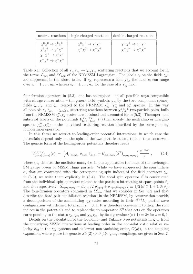
neutral reactions single-charged reactions double-charged reactions
χ0χ0 → χ0χ0 χ0χ+ → χ0χ+ χ+χ+ → χ+χ+
χ0χ0 → χ−χ+ χ−χ0 → χ−χ0 χ−χ− → χ−χ−
χ−χ+ → χ0χ0
χ−χ+ → χ−χ+
Table 5.1: Collection of all χe1χe2 → χe4χe3 scattering reactions that we account for inthe terms Lpot and δLann of the NRMSSM Lagrangian. The labels ei on the fields χeiare suppressed in the above table. If χei represents a field χ0
ei, the label ei can range
over ei = 1, . . . , n0, whereas ei = 1, . . . , n+ for the case of a χ±eifield.
four-fermion operators in (5.3), one has to replace – in all possible ways compatiblewith charge conservation – the generic field symbols χei by the (two-component spinor)fields ξei, ηei and ζei, related to the NRMSSM χ0
ei, χ−
eiand χ+
eispecies. In this way
all possible χe1χe2 → χe4χe3 scattering reactions between χ0/χ± two-particle pairs, builtfrom the NRMSSM χ0
i , χ±j states, are obtained and accounted for in (5.3). The super- and
subscript labels on the potentials V χχ→χχe1e2e4e3(r) then specify the neutralino or chargino
species (χ0ei, χ±
ei) in the individual scattering reaction described by the corresponding
four-fermion operator.In this thesis we restrict to leading-order potential interactions, in which case the
potentials depend only on the spin of the two-particle states, that is thus conserved.The generic form of the leading-order potentials therefore reads
V χχ→χχe1e2e4e3(r) =
(Ae1e2e4e3 δα4α1
δα3α2+Be1e2e4e3
(~S 2)α4α1,α3α2
) e−mφr
r, (5.4)
where mφ denotes the mediator mass, i.e. in our application the mass of the exchangedSM gauge boson or MSSM Higgs particle. While we have suppressed the spin indicesαi that are contracted with the corresponding spin indices of the field operators χeiin (5.3), we write them explicitly in (5.4). The total spin operator ~S is constructedfrom the individual spin-operators related to the particles interacting at space-points ~x1and ~x2, respectively: ~Sα4α1,α3α2
= ~σα4α1/2 δα3α2
+ δα4α1~σα3α2
/2 ≡ 1/2 (~σ ⊗ 1 + 1 ⊗ ~σ).The four-fermion operators contained in δLann that we consider in Sec. 5.2 and thatdescribe the hard pair-annihilation reactions in the NRMSSM, by construction providea decomposition of the annihilating χχ-states according to their 2S+1LJ partial-waveconfiguration with defined total spin s = 0, 1. It is therefore convenient to drop the spinindices in the potentials and to replace the spin-operator ~S 2 that acts on the operatorscorresponding to the states χe1χe2 and χe4χe3 , by its eigenvalue s(s+1) = 2s for s = 0, 1.
Details on the calculation of the Coulomb- and Yukawa-type potentials in Lpot fromthe underlying MSSM interactions at leading order in the non-relativistic relative ve-locity vrel in the χχ systems and at lowest non-vanishing order, O(g2i ), in the couplingexpansion, where gi are the generic SU(2)L×U(1)Y gauge couplings, are given in Sec. 7.
74
Regarding the short-distance annihilation reactions in the effective theory, to be discussedin the next section and in Chap. 6, we take up to O(v2rel) corrections in the velocity ex-pansion in the effective theory into account, while we work at lowest non-vanishing order,O(g4i ), in the expansion in the couplings.
5.2 χ0/χ± pair-annihilations in the NRMSSM
Within the NRMSSM, we aim to describe neutralino and chargino pair-annihilationprocesses into two-particle final states of Standard Model and (light) Higgs particles,which are not non-relativistic. The theory will contain effects from virtual and higher-mass Higgs and SUSY particle modes as well, encoded in the EFT operator coefficientsand parameters. Let us note that the framework presented here is not suited to studys-channel resonance-enhanced rates when accounting at the same time for Sommerfeldenhancements.1 For this reason we have to choose models without s-channel resonantenhancement for our analysis of Sommerfeld enhancements in neutralino and chargino co-annihilation rates in Chap. 9. Finally, we exclude the case of accidental mass degeneraciesof further SUSY particles with the set of non-relativistic neutralinos and charginos. Anextension of the effective theory framework to include sfermion or Higgs states that arenearly mass-degenerate with the χ0/χ± species in the NRMSSM and can therefore havean impact on the χ0
1 relic density through co-annihilation effects is straightforward butbeyond the scope of this thesis.
The hard pair-annihilation reactions of heavy non-relativistic neutralinos and charg-inos produce SM and light Higgs particle final states that are not described withinthe non-relativistic effective theory, as these final states are characterised by velocitiesoutside the non-relativistic regime. However, since the hard inclusive pair-annihilationprocesses take place within distances of order 1/mLSP, we can incorporate the short-distance annihilation rates of non-relativistic neutralinos and charginos in the effectivetheory through the absorptive part of Wilson coefficients of local four-fermion operatorsin δLann, following the approach of [30]. The full annihilation rates in the non-relativisticeffective theory are then given by the absorptive part of the matrix elements of thesefour-fermion operators. While the matrix elements of the operators themselves mayencode long-distance effects, giving rise to Sommerfeld enhancements, the contributionto the hard annihilation reaction factors out in the form of the Wilson coefficient.
Let us see in more detail how this formalism is applied to our case: In contrast
1As regards the short-distance (tree-level) annihilation rates, results for the specific case of resonant s-channel annihilation reactions can be obtained from our analytic expressions for the Wilson coefficients inδLann (collected in Appendix A) by adding a resonance width to the corresponding s-channel propagator.This is because the hard rates result from an on-shell matching involving an expansion around the massscale set by the annihilating particle states (see Sec. 6.1). However, the treatment of both Sommerfeldenhancements and resonant s-channel annihilation requires that the corresponding s-channel propagatoris expanded around the mass scale set by the initially incoming two-particle state instead of the actuallyannihilating states. A proper treatment of s-channel resonances in Sommerfeld-enhanced annihilationrates is therefore more involved and requires modifications of our set-up.
75
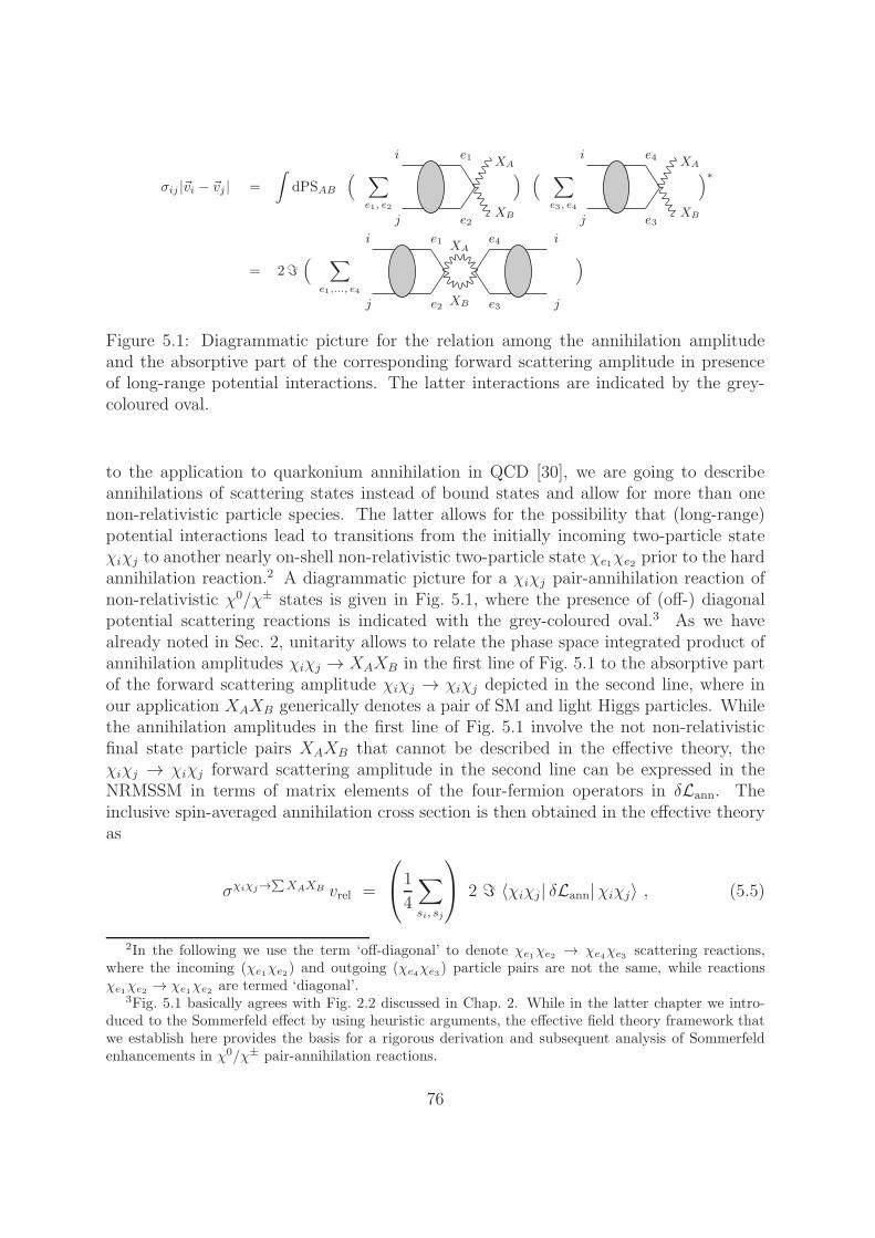
σij |~vi − ~vj | =
∫dPSAB
( ∑
e1, e2
i
j
e1
e2
XA
XB
) ( ∑
e3, e4
i
j
e4
e3
XA
XB
)∗
= 2ℑ( ∑
e1,..., e4
i
j
e1
e2
i
j
e4
e3
XA
XB
)
Figure 5.1: Diagrammatic picture for the relation among the annihilation amplitudeand the absorptive part of the corresponding forward scattering amplitude in presenceof long-range potential interactions. The latter interactions are indicated by the grey-coloured oval.
to the application to quarkonium annihilation in QCD [30], we are going to describeannihilations of scattering states instead of bound states and allow for more than onenon-relativistic particle species. The latter allows for the possibility that (long-range)potential interactions lead to transitions from the initially incoming two-particle stateχiχj to another nearly on-shell non-relativistic two-particle state χe1χe2 prior to the hardannihilation reaction.2 A diagrammatic picture for a χiχj pair-annihilation reaction ofnon-relativistic χ0/χ± states is given in Fig. 5.1, where the presence of (off-) diagonalpotential scattering reactions is indicated with the grey-coloured oval.3 As we havealready noted in Sec. 2, unitarity allows to relate the phase space integrated product ofannihilation amplitudes χiχj → XAXB in the first line of Fig. 5.1 to the absorptive partof the forward scattering amplitude χiχj → χiχj depicted in the second line, where inour application XAXB generically denotes a pair of SM and light Higgs particles. Whilethe annihilation amplitudes in the first line of Fig. 5.1 involve the not non-relativisticfinal state particle pairs XAXB that cannot be described in the effective theory, theχiχj → χiχj forward scattering amplitude in the second line can be expressed in theNRMSSM in terms of matrix elements of the four-fermion operators in δLann. Theinclusive spin-averaged annihilation cross section is then obtained in the effective theoryas
σχiχj→∑XAXB vrel =
1
4
∑
si, sj
2 ℑ 〈χiχj| δLann|χiχj〉 , (5.5)
2In the following we use the term ‘off-diagonal’ to denote χe1χe2 → χe4χe3 scattering reactions,where the incoming (χe1χe2) and outgoing (χe4χe3) particle pairs are not the same, while reactionsχe1χe2 → χe1χe2 are termed ‘diagonal’.
3Fig. 5.1 basically agrees with Fig. 2.2 discussed in Chap. 2. While in the latter chapter we intro-duced to the Sommerfeld effect by using heuristic arguments, the effective field theory framework thatwe establish here provides the basis for a rigorous derivation and subsequent analysis of Sommerfeldenhancements in χ0/χ± pair-annihilation reactions.
76

with vrel = |~vi − ~vj | the relative velocity of the annihilating particles in the centre-of-mass frame. The matrix elements4 of the four-fermion operators in δLann account forthe (off-) diagonal long-range potential interactions between the non-relativistic χχ pairsprior to annihilation, which causes the Sommerfeld effect. The information on the hardannihilation reactions into all accessible XAXB final states is contained in the Wilsoncoefficients of the operators, implying that the factorisation of long-range and short-distance effects becomes manifest in the effective theory. Due to the presence of theoff-diagonal long-range potential interactions, the hard annihilation reactions, encodedin the Wilson coefficients, are determined by the absorptive part of χe1χe2 → χe4χe3amplitudes, as can be seen in the second line of Fig. 5.1. It is worth to stress thatthe χe1χe2 particle pair is not necessarily equal to the χe4χe3 pair, such that apartfrom true forward scattering reactions χe1χe2 → χe1χe2 , we encounter off-diagonal hardχe1χe2 → χe4χe3 reactions as well.
In the following subsections we discuss the terms in δLann that describe the absorp-tive part of hard χe1χe2 → χe4χe3 scattering reactions in the effective theory includingO(v2rel) corrections. The dimension-6 four-fermion operators given in Sec. 5.2.1 pro-vide the leading, O(v0rel), terms in the non-relativistic expansion of hard (off-) diagonalχ0/χ± pair-annihilations rates. Dimension-8 four fermion operators in Sec. 5.2.2, relatedto P - and next-to-next-to-leading order S-wave reactions, then allow to give the corre-sponding O(v2rel) corrections in the velocity expansion. We give the explicit expressionsof four-fermion operators in δLann and discuss generic properties of the correspondingWilson coefficients. The actual determination of these Wilson coefficients, at lowestnon-vanishing order in the expansion in coupling factors, from a MSSM matching calcu-lation is postponed to Sec. 6.1. Note that the lowest non-vanishing order in the couplingexpansion, O(α2
i ), where αi = g2i /4π, corresponds to tree-level annihilation processes.In this case the annihilation rates can be given separately for every exclusive SM orHiggs two-particle final state XAXB, since the tree-level processes are free from infrareddivergencies. In higher orders in the couplings the formalism applies to the inclusiveannihilation cross section [30] or to suitably defined infrared-safe final states.
5.2.1 Basis of dimension-6 operators in δLann
The leading-order contributions in δLann are given by dimension-6 four-fermion opera-tors. For instance, the specific dimension-6 four-fermion operator that encodes scatteringof a non-relativistic incoming neutralino pair χ0
1χ01 in an 1S0 partial-wave state into an
outgoing χ01χ
01 state in the same 1S0 partial-wave configuration is given by
δLd=6ann ⊃
1
4fχ
0χ0→χ0χ0
1111 (1S0) ξ†1 ξc1 ξc†1 ξ1 , (5.6)
4In order to make contact with the commonly used notation in quarkonium annihilation, we abusenotation when writing in (5.5) the matrix element of δLann instead of the corresponding forward scat-tering amplitude. Written properly, the matrix element on the right-hand side in (5.5) should involvethe position-space integration over the interaction Lagrangian,
∫d4x δLann(x), which implies that an
additional factor (2π)4δ(4)(pfinal−pinitial) arises when evaluating the matrix element. This factors shouldhowever not be included in the relation (5.5).
77
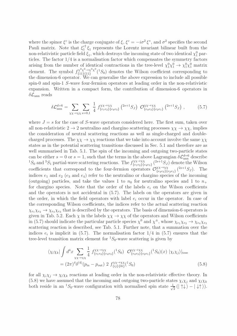
where the spinor ξc is the charge conjugate of ξ, ξc = −iσ2 ξ∗, and σ2 specifies the secondPauli matrix. Note that ξc†1 ξ1 represents the Lorentz invariant bilinear built from thenon-relativistic particle field ξ1, which destroys the incoming state of two identical χ0
1 par-ticles. The factor 1/4 is a normalisation factor which compensates the symmetry factorsarising from the number of identical contractions in the tree-level χ0
1χ01 → χ0
1χ01 matrix
element. The symbol fχ0χ0→χ0χ0
1111 (1S0) denotes the Wilson coefficient corresponding tothe dimension-6 operator. We can generalise the above expression to include all possiblespin-0 and spin-1 S -wave four-fermion operators at leading order in the non-relativisticexpansion. Written in a compact form, the contribution of dimension-6 operators inδLann reads
δLd=6ann =
∑
χχ→χχ
∑
s=0,1
1
4fχχ→χχe1e2e4e3
(2s+1SJ
)Oχχ→χχ
e4e3e2e1(2s+1SJ
), (5.7)
where J = s for the case of S-wave operators considered here. The first sum, taken overall non-relativistic 2→ 2 neutralino and chargino scattering processes χχ→ χχ, impliesthe consideration of neutral scattering reactions as well as single-charged and double-charged processes. The χχ→ χχ reactions that we take into account involve the same χχstates as in the potential scattering transitions discussed in Sec. 5.1 and therefore are aswell summarised in Tab. 5.1. The spin of the incoming and outgoing two-particle statescan be either s = 0 or s = 1, such that the terms in the above Lagrangian δLd=6
ann describe1S0 and
3S1 partial-wave scattering reactions. The fχχ→χχe1e2e4e3 (
2s+1SJ) denote the Wilson
coefficients that correspond to the four-fermion operators Oχχ→χχe4e3e2e1 (
2s+1SJ). The
indices e1 and e2 (e3 and e4) refer to the neutralino or chargino species of the incoming(outgoing) particles, and take the values 1 to n0 for neutralino species and 1 to n+
for chargino species. Note that the order of the labels ei on the Wilson coefficientsand the operators is not accidental in (5.7). The labels on the operators are given inthe order, in which the field operators with label ei occur in the operator. In case ofthe corresponding Wilson coefficients, the indices refer to the actual scattering reactionχe1χe2 → χe4χe3 that is described by the operators. The basis of dimension-6 operators isgiven in Tab. 5.2. Each χ in the labels χχ→ χχ of the operators and Wilson coefficientsin (5.7) should indicate the particular particle species χ0 and χ±, whose χe1χe2 → χe4χe3scattering reaction is described, see Tab. 5.1. Further note, that a summation over theindices ei is implicit in (5.7). The normalisation factor 1/4 in (5.7) ensures that thetree-level transition matrix element for 1S0-wave scattering is given by
〈χlχk|∫d4x
∑
χχ→χχ
1
4fχχ→χχe1e2e4e3(
1S0) Oχχ→χχe4e3e2e1(
1S0)(x) |χiχj〉|tree
= (2π)4δ(4)(pin − pout) 2 fχχ→χχijlk(
1S0) (5.8)
for all χiχj → χlχk reactions at leading order in the non-relativistic effective theory. In(5.8) we have assumed that the incoming and outgoing two-particle states χiχj and χlχkboth reside in an 1S0-wave configuration with normalised spin state 1√
2(| ↑↓ 〉 − | ↓↑ 〉).
78

χe1χe2 → χe4χe3 Oχχ→χχe4e3e2e1 (
1S0) Oχχ→χχe4e3e2e1 (
3S1)
χ0 χ0 → χ0 χ0 ξ†e4 ξce3
ξc†e2 ξe1 ξ†e4~σξce3
ξc†e2~σ ξe1
χ0 χ0 → χ−χ+ η†e4 ζce3
ξc†e2 ξe1 η†e4~σζce3
ξc†e2~σ ξe1
χ−χ+ → χ0 χ0 ξ†e4 ξce3
ζc†e2 ηe1 ξ†e4~σξce3
ζc†e2~σ ηe1
χ−χ+ → χ−χ+ η†e4 ζce3 ζc†e2 ηe1 η†e4~σζ
ce3 ζc†e2~σ ηe1
χ0χ+ → χ0χ+ ξ†e4 ζce3
ζc†e2 ξe1 ξ†e4~σζce3
ζc†e2~σ ξe1
χ−χ0 → χ−χ0 η†e4 ξce3
ξc†e2 ηe1 η†e4~σξce3
ξc†e2~σ ηe1
χ+χ+ → χ+χ+ ζ†e4 ζce3
ζc†e2 ζe1 ζ†e4~σζce3
ζc†e2~σ ζe1
χ−χ− → χ−χ− η†e4 ηce3
ηc†e2 ηe1 η†e4~σηce3
ηc†e2~σ ηe1
Table 5.2: Four-fermion operators for leading-order S-wave χe1χe2 → χe4χe3 transitions.The indices ei, i = 1, . . . , 4 on the χ-fields are suppressed in the first column. In additionto the specified operators there are redundant ones, which are obtained by interchangingthe field-operator symbols ξ, η or ζ (but not the labels) at the first and second and/or thethird and fourth position in the operator Oχχ→χχ. For example, for 1S0 χ
0χ+ → χ0χ+
operators one of the three classes of field-interchanged operators is given by the 1S0
χ+χ0 → χ+χ0 operators ζ†e4 ξce3ξc†e2 ζe1.
A similar relation for the tree-level transition matrix element of 3S1-wave scattering inthe effective theory holds for all χiχj → χlχk reactions. Note that in order to derive (5.8)one has to take into account relations among Wilson coefficients of different operators,which will be deduced in the next paragraph.
There are redundancies in δLd=6ann , (5.7), as several operators can describe one specific
scattering reaction with a χe1 and a χe2 (χe4 and χe3) particle in the initial (final) state.This redundancy is associated with operators that arise from interchanging the single-particle field operators at the first and second and/or third and fourth position in agiven Oχχ→χχ. The corresponding Wilson coefficients are related to each other, as theyencode the same information on a given specific scattering reaction. Consequently, theredundancy manifests itself in symmetry relations among the Wilson coefficients underexchange of the labels e1 ↔ e2 and/or e4 ↔ e3. These relations read
fχe2
χe1→χe4
χe3
e2e1e4e3(2s+1SJ
)= ηs f
χe1χe2
→χe4χe3
e1e2e4e3(2s+1SJ
),
fχe1
χe2→χe3
χe4
e1e2e3e4(2s+1SJ
)= ηs f
χe1χe2
→χe4χe3
e1e2e4e3(2s+1SJ
), (5.9)
with
ηs =
1 for s = 0
−1 for s = 1. (5.10)
79
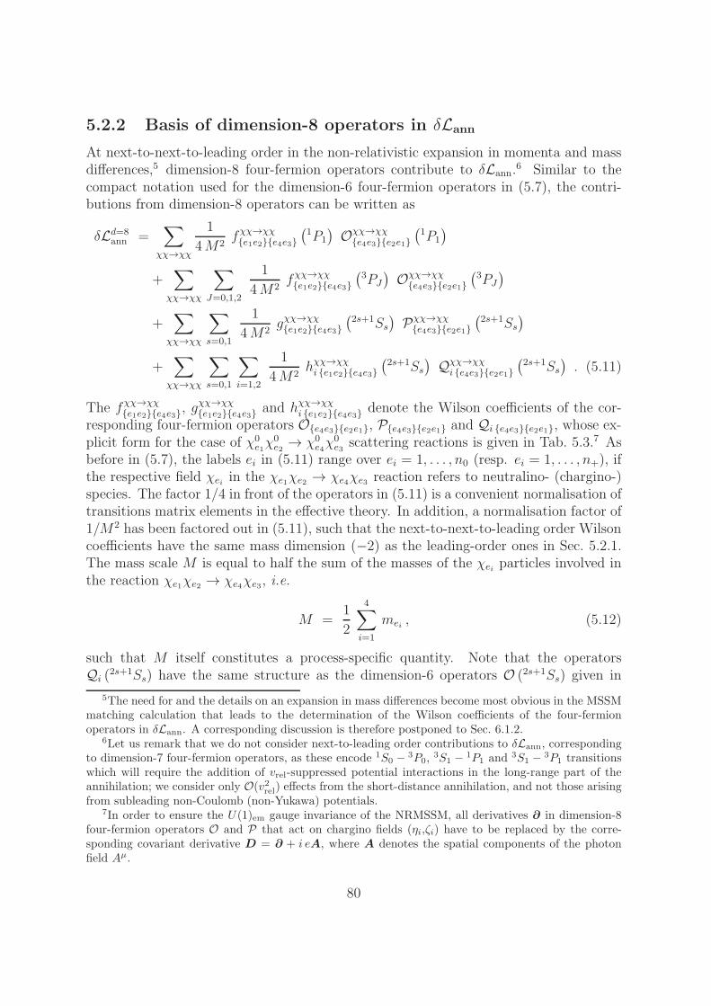
5.2.2 Basis of dimension-8 operators in δLann
At next-to-next-to-leading order in the non-relativistic expansion in momenta and massdifferences,5 dimension-8 four-fermion operators contribute to δLann.
6 Similar to thecompact notation used for the dimension-6 four-fermion operators in (5.7), the contri-butions from dimension-8 operators can be written as
δLd=8ann =
∑
χχ→χχ
1
4M2fχχ→χχe1e2e4e3
(1P1
)Oχχ→χχ
e4e3e2e1(1P1
)
+∑
χχ→χχ
∑
J=0,1,2
1
4M2fχχ→χχe1e2e4e3
(3PJ)Oχχ→χχ
e4e3e2e1(3PJ)
+∑
χχ→χχ
∑
s=0,1
1
4M2gχχ→χχe1e2e4e3
(2s+1Ss
)Pχχ→χχ
e4e3e2e1(2s+1Ss
)
+∑
χχ→χχ
∑
s=0,1
∑
i=1,2
1
4M2hχχ→χχi e1e2e4e3
(2s+1Ss
)Qχχ→χχi e4e3e2e1
(2s+1Ss
). (5.11)
The fχχ→χχe1e2e4e3, g
χχ→χχe1e2e4e3 and hχχ→χχ
i e1e2e4e3 denote the Wilson coefficients of the cor-responding four-fermion operators Oe4e3e2e1, Pe4e3e2e1 and Qi e4e3e2e1, whose ex-plicit form for the case of χ0
e1χ0e2 → χ0
e4χ0e3 scattering reactions is given in Tab. 5.3.7 As
before in (5.7), the labels ei in (5.11) range over ei = 1, . . . , n0 (resp. ei = 1, . . . , n+), ifthe respective field χei in the χe1χe2 → χe4χe3 reaction refers to neutralino- (chargino-)species. The factor 1/4 in front of the operators in (5.11) is a convenient normalisation oftransitions matrix elements in the effective theory. In addition, a normalisation factor of1/M2 has been factored out in (5.11), such that the next-to-next-to-leading order Wilsoncoefficients have the same mass dimension (−2) as the leading-order ones in Sec. 5.2.1.The mass scale M is equal to half the sum of the masses of the χei particles involved inthe reaction χe1χe2 → χe4χe3, i.e.
M =1
2
4∑
i=1
mei , (5.12)
such that M itself constitutes a process-specific quantity. Note that the operatorsQi (2s+1Ss) have the same structure as the dimension-6 operators O (2s+1Ss) given in
5The need for and the details on an expansion in mass differences become most obvious in the MSSMmatching calculation that leads to the determination of the Wilson coefficients of the four-fermionoperators in δLann. A corresponding discussion is therefore postponed to Sec. 6.1.2.
6Let us remark that we do not consider next-to-leading order contributions to δLann, correspondingto dimension-7 four-fermion operators, as these encode 1S0 − 3P0,
3S1 − 1P1 and 3S1 − 3P1 transitionswhich will require the addition of vrel-suppressed potential interactions in the long-range part of theannihilation; we consider only O(v2rel) effects from the short-distance annihilation, and not those arisingfrom subleading non-Coulomb (non-Yukawa) potentials.
7In order to ensure the U(1)em gauge invariance of the NRMSSM, all derivatives ∂ in dimension-8four-fermion operators O and P that act on chargino fields (ηi,ζi) have to be replaced by the corre-sponding covariant derivative D = ∂ + i eA, where A denotes the spatial components of the photonfield Aµ.
80
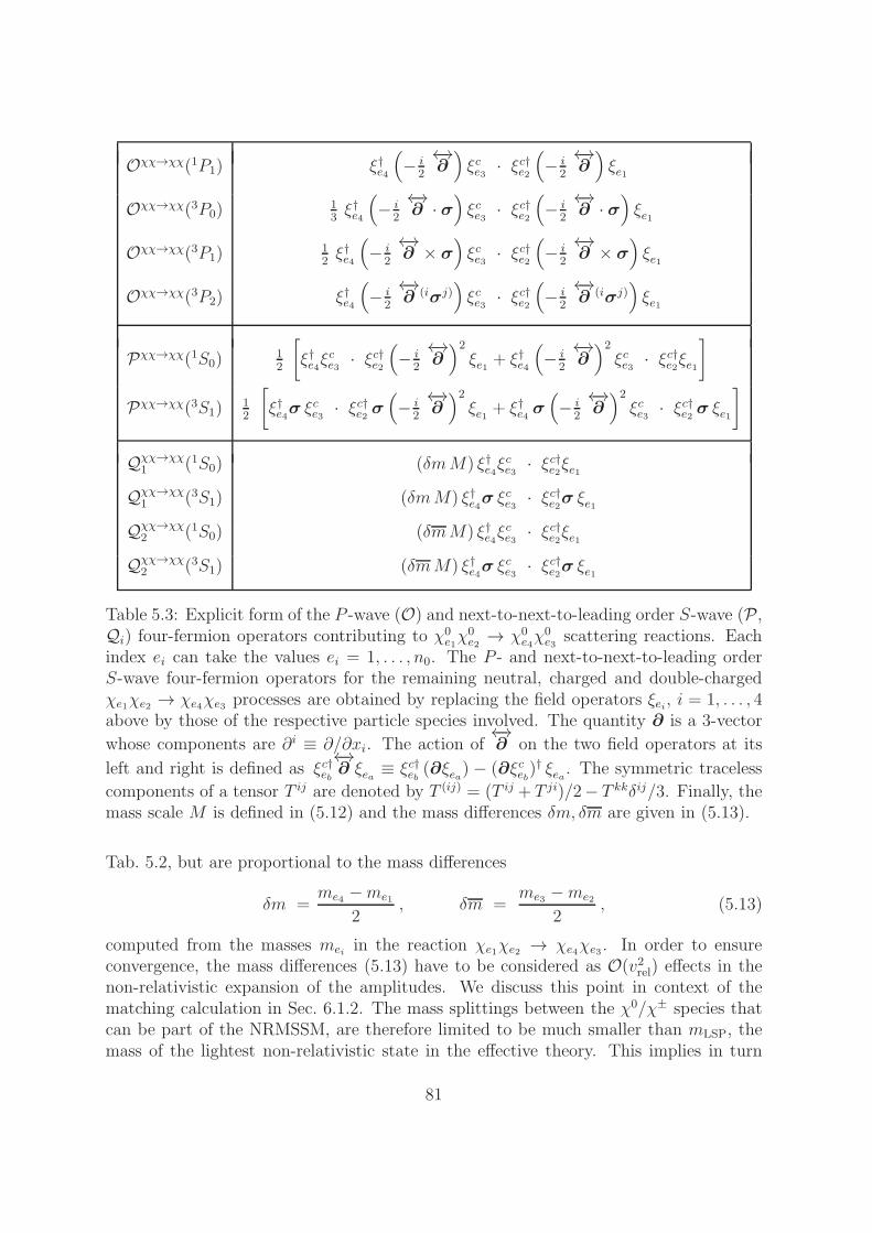
Oχχ→χχ(1P1) ξ†e4
(− i
2
←→∂)ξce3 · ξc†e2
(− i
2
←→∂)ξe1
Oχχ→χχ(3P0)13ξ†e4
(− i
2
←→∂ · σ
)ξce3 · ξc†e2
(− i
2
←→∂ · σ
)ξe1
Oχχ→χχ(3P1)12ξ†e4
(− i
2
←→∂ × σ
)ξce3 · ξc†e2
(− i
2
←→∂ × σ
)ξe1
Oχχ→χχ(3P2) ξ†e4
(− i
2
←→∂ (iσj)
)ξce3 · ξc†e2
(− i
2
←→∂ (iσj)
)ξe1
Pχχ→χχ(1S0)12
[ξ†e4ξ
ce3 · ξc†e2
(− i
2
←→∂)2ξe1 + ξ†e4
(− i
2
←→∂)2ξce3 · ξc†e2ξe1
]
Pχχ→χχ(3S1)12
[ξ†e4σ ξ
ce3 · ξc†e2 σ
(− i
2
←→∂)2ξe1 + ξ†e4 σ
(− i
2
←→∂)2ξce3 · ξc†e2 σ ξe1
]
Qχχ→χχ1 (1S0) (δmM) ξ†e4ξ
ce3· ξc†e2ξe1
Qχχ→χχ1 (3S1) (δmM) ξ†e4σ ξ
ce3· ξc†e2σ ξe1
Qχχ→χχ2 (1S0) (δmM) ξ†e4ξ
ce3· ξc†e2ξe1
Qχχ→χχ2 (3S1) (δmM) ξ†e4σ ξ
ce3 · ξc†e2σ ξe1
Table 5.3: Explicit form of the P -wave (O) and next-to-next-to-leading order S-wave (P,Qi) four-fermion operators contributing to χ0
e1χ0e2 → χ0
e4χ0e3 scattering reactions. Each
index ei can take the values ei = 1, . . . , n0. The P - and next-to-next-to-leading orderS-wave four-fermion operators for the remaining neutral, charged and double-chargedχe1χe2 → χe4χe3 processes are obtained by replacing the field operators ξei, i = 1, . . . , 4above by those of the respective particle species involved. The quantity ∂ is a 3-vector
whose components are ∂i ≡ ∂/∂xi. The action of←→∂ on the two field operators at its
left and right is defined as ξc†eb←→∂ ξea ≡ ξc†eb (∂ξea) − (∂ξceb)
† ξea. The symmetric traceless
components of a tensor T ij are denoted by T (ij) = (T ij + T ji)/2− T kkδij/3. Finally, themass scale M is defined in (5.12) and the mass differences δm, δm are given in (5.13).
Tab. 5.2, but are proportional to the mass differences
δm =me4 −me1
2, δm =
me3 −me2
2, (5.13)
computed from the masses mei in the reaction χe1χe2 → χe4χe3 . In order to ensureconvergence, the mass differences (5.13) have to be considered as O(v2rel) effects in thenon-relativistic expansion of the amplitudes. We discuss this point in context of thematching calculation in Sec. 6.1.2. The mass splittings between the χ0/χ± species thatcan be part of the NRMSSM, are therefore limited to be much smaller than mLSP, themass of the lightest non-relativistic state in the effective theory. This implies in turn
81
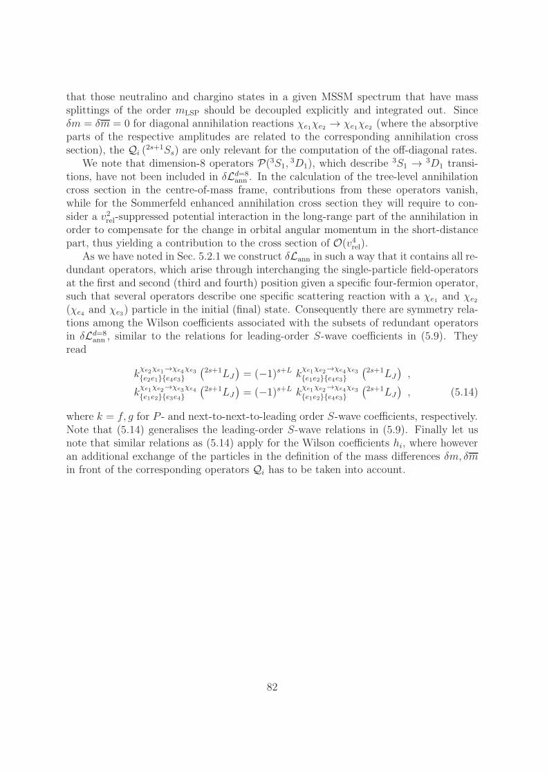
that those neutralino and chargino states in a given MSSM spectrum that have masssplittings of the order mLSP should be decoupled explicitly and integrated out. Sinceδm = δm = 0 for diagonal annihilation reactions χe1χe2 → χe1χe2 (where the absorptiveparts of the respective amplitudes are related to the corresponding annihilation crosssection), the Qi (2s+1Ss) are only relevant for the computation of the off-diagonal rates.
We note that dimension-8 operators P(3S1,3D1), which describe 3S1 → 3D1 transi-
tions, have not been included in δLd=8ann . In the calculation of the tree-level annihilation
cross section in the centre-of-mass frame, contributions from these operators vanish,while for the Sommerfeld enhanced annihilation cross section they will require to con-sider a v2rel-suppressed potential interaction in the long-range part of the annihilation inorder to compensate for the change in orbital angular momentum in the short-distancepart, thus yielding a contribution to the cross section of O(v4rel).
As we have noted in Sec. 5.2.1 we construct δLann in such a way that it contains all re-dundant operators, which arise through interchanging the single-particle field-operatorsat the first and second (third and fourth) position given a specific four-fermion operator,such that several operators describe one specific scattering reaction with a χe1 and χe2(χe4 and χe3) particle in the initial (final) state. Consequently there are symmetry rela-tions among the Wilson coefficients associated with the subsets of redundant operatorsin δLd=8
ann , similar to the relations for leading-order S-wave coefficients in (5.9). Theyread
kχe2
χe1→χe4
χe3
e2e1e4e3(2s+1LJ
)= (−1)s+L kχe1
χe2→χe4
χe3
e1e2e4e3(2s+1LJ
),
kχe1
χe2→χe3
χe4
e1e2e3e4(2s+1LJ
)= (−1)s+L kχe1
χe2→χe4
χe3
e1e2e4e3(2s+1LJ
), (5.14)
where k = f, g for P - and next-to-next-to-leading order S-wave coefficients, respectively.Note that (5.14) generalises the leading-order S-wave relations in (5.9). Finally let usnote that similar relations as (5.14) apply for the Wilson coefficients hi, where howeveran additional exchange of the particles in the definition of the mass differences δm, δmin front of the corresponding operators Qi has to be taken into account.
82
Chapter 6
The hard annihilation reactions
In Chap. 5 we have introduced the NRMSSM, an effective field theory that is de-signed to describe scattering and annihilation reactions of non-relativistic neutralinos andcharginos. Here we will focus on the hard pair-annihilation reactions of non-relativisticχ0/χ± states in the effective theory, which are encoded in the absorptive part of the Wil-son coefficients of four-fermion operators in δLann, a part of the generic EFT LagrangianLNRMSSM. Conceptually this chapter is divided into three parts. The first part comprisesSec. 6.1 and contains the technical details on the calculation of our purely analytic ex-pressions for the absorptive parts of the Wilson coefficients. We describe the steps in thecalculation of the coefficients related to leading-order S-wave, P - and next-to-next-toleading order S-wave annihilation processes and collect explicit analytic expressions forthe coefficients in terms of the underlying MSSM parameters and couplings in Appen-dices A.1–A.3. Sec. 6.2 covers the second part, where we provide an extensive discussionon the numerical comparison of the hard (tree-level) annihilation cross sections derivedin the NRMSSM with results from the numerical code MadGraph [89]. The thirdpart is contained in Sec. 6.3. Here we illustrate in an analytic sample calculation inthe pure-wino NRMSSM, how the generic results for the Wilson coefficients, collectedin Appendices A.1–A.3, have to be applied in order to obtain all (off-) diagonal hardco-annihilation rates in this scenario.
The structure of the first part is as follows. The matching condition that relatesthe perturbative χiχj → χlχk scattering amplitudes in the NRMSSM with the corre-sponding amplitudes in the MSSM and thereby allows the determination of the Wilsoncoefficients in δLann in terms of the underlying MSSM parameters and couplings is dis-cussed in Sec. 6.1.1. The matching procedure requires an expansion of the MSSM ampli-tudes in the non-relativistic external momenta. In addition, as we generically considerprocesses χe1χe2 → χe4χe3 where the outgoing two-particle states can be different andslightly lighter or heavier than the incoming ones, we have to perform an expansion inmass differences of the states involved. We commend on these expansions in Sec. 6.1.2.Subsequently we give a brief discussion on the gauge used in the calculation in Sec. 6.1.3.Further details on the actual determination through the MSSM matching calculation andthe final form of the Wilson coefficients are provided in Sec. 6.1.4, including a master
83
formula for the Wilson coefficients in terms of coupling and kinematic factors. Resultsand recipes for the construction of these coupling and kinematic factors, valid in thegeneral MSSM, are collected in Appendices A.1–A.3.
In the second part we discuss the numerical comparison of our non-relativistic ap-proximation to χ0/χ± pair-annihilation cross sections σvrel with corresponding resultsproduced with MadGraph. To this end we select several annihilation processes wherethe role of the next-to-next-to-leading corrections from our analytic calculation of theannihilation cross section is markedly different. In Sec. 6.2.1 we present two reactionswhere P - and next-to-next-to-leading S-wave contributions are of the same order. TwoS-wave dominated reactions are considered in Sec. 6.2.2, followed by a P -wave domi-nated process in Sec. 6.2.3. The case of an off-diagonal rate, where no numerical checkwith MadGraph is available, is given in Sec. 6.2.4. As our effective field theory frame-work allows to describe annihilation rates of “hydrogen-like” χχ states as well, we con-clude by comparing results for annihilation reactions of two such “hydrogen-like” stateswith MadGraph generated data in Sec. 6.2.5. The examples of Sec. 6.2 in particu-lar illustrate the importance of separating the different partial-wave contributions to theshort-distance annihilation in view of the computation of the Sommerfeld-corrected crosssections, including O(v2rel) corrections to the hard annihilation rates.1
In the third part we first provide in Sec. 6.3.1 a detailed derivation of the coupling fac-tor expressions needed in the construction of the Wilson coefficients in non-relativisticχ+1 χ
−1 → W+W− annihilations in the pure-wino NRMSSM. Subsequently the corre-
sponding kinematic factor expressions are derived in Sec. 6.3.2. In both sections we relyon the conventions and notations introduced in Appendices A.1–A.3. Finally, Sec. 6.3.3contains analytic results for all exclusive tree-level co-annihilation rates in the pure-winoNRMSSM at O(v2rel), that are relevant in the relic abundance calculation in this scenario.
6.1 Matching calculation & Master formula
6.1.1 Matching condition
The Wilson coefficients of the four-fermion operators in δLann are determined by thematching condition
A(χiχj → χlχk) |MSSM, perturbative =∑ 1
4Md−6f(d)χχ→χχe1e2e4e3(
2s+1LJ)
× 〈χlχk| O(d)χχ→χχe4e3e2e1(
2s+1LJ) |χiχj〉 |NRMSSM, perturbative . (6.1)
1The investigation of Sommerfeld enhancements in some popular MSSM scenarios is the contentof Chap. 9, where we find that Sommerfeld-enhanced P - and next-to-next-to-leading order S-wavecorrections to the hard annihilation rates play a subdominant role in the relic abundance calculationas compared to the effect from correctly accounting for off-diagonal (leading-order S-wave) annihilationrates. The latter turns out to be particularly crucial in an accurate calculation of the χ0
1 relic densityincluding Sommerfeld enhancements, as we discuss in detail in Chap. 9.
84
Here we have denoted the dimension-d four-fermion operators and their correspondingWilson coefficients with symbols O(d) and f (d) in order to make the notation of thematching condition – which in particular implies a summation
∑d≥6 – simpler. The
connection to the notation established in Chap. 5 is obvious. For instance we have thecorrespondence O(d=6)(1S0) = O(1S0) and f
(d=6)(1S0) = f(1S0) as well as O(d=8)(1S0) =P(1S0) and f
(d=8)(1S0) = g(1S0). Except for this section (Sec. 6.1), we will always usethe notation from Chap. 5 and denote the Wilson coefficients of dimension d = 6 andd = 8 operators by f(2s+1Ss) and f(
2s+1PJ), g(2s+1Ss), hi(
2s+1Ss), respectively. The sameapplies to the notation for the dimension d = 6, 8 four-fermion operators. Recall thatthe mass scale M , defined in (5.12), is a χe1χe2 → χe4χe3 process-specific quantity. Letus finally note that any Wilson coefficient f (d) in (6.1) generically has mass dimension−2, independent of the mass dimension d of the corresponding four-fermion operator.
For equation (6.1) to hold, we have to use the same (non-relativistic) normalisationof the incoming and outgoing states in both the full theory and the NRMSSM. Formallythis condition is a generalisation and appropriate modification of the matching conditionset up in [30], therein used for the determination of the Wilson coefficients of four fermionoperators in the NRQCD Lagrangian. Here we will determine the contributions to theWilson coefficients in δLann that describe the tree-level annihilation reactions of χ0/χ±
pairs into exclusive SM and light Higgs two-body final states XAXB, which we shalldenote as f (d)χχ→XAXB→χχ(2s+1LJ ). The unitarity of the S-matrix at the diagrammaticlevel establishes a relation among the tree-level annihilation rate for χiχj → XAXB andthe imaginary part of the 1-loop forward-scattering reaction χiχj → XAXB → χiχj :
∫[dPSAB] |A(χiχj → XAXB)|2 = 2 ℑ [A(χiχj → XAXB → χiχj)] (6.2)
= 2∑ 1
4Md−6ℑ[f(d)χχ→XAXB→χχe1e2e4e3 (2s+1LJ)
]〈χiχj |O(d)χχ→χχ
e4e3e2e1(2s+1LJ )|χiχj〉 .
We generalise this relation and define the absorptive part of the (off-) diagonal amplitudeA(χiχj → XAXB → χlχk) as well as the absorptive part of the Wilson coefficients inthe following way:
∫[dPSAB] A(χiχj → XAXB)×A(χlχk → XAXB)
∗ (6.3)
= 2 [A(χiχj → XAXB → χlχk)] |absorptive
= 2∑ 1
4Md−6f(d)χχ→XAXB→χχe1e2e4e3 (2s+1LJ) 〈χlχk|O(d)χχ→χχ
e4e3e2e1(2s+1LJ)|χiχj〉 ,
where we have introduced the notation
f(d)χχ→XAXB→χχijlk (2s+1LJ) = f
(d)χχ→XAXB→χχijlk (2s+1LJ) |absorptive . (6.4)
With this definition, the absorptive part of a Wilson coefficient that encodes a χiχj →χiχj forward-scattering reaction coincides with its imaginary part. The adjoint of the
85
four-fermion operators in δLann that do not involve mass differences δm, δm in theirdefinition satisfy
O(d) †e4e3e2e1(
2s+1LJ) = O(d)e1e2e3e4(
2s+1LJ) , (6.5)
which for dimension-d operators with d = 6, 8 is easily seen from the explicit expressionsin Tab. 5.2 and Tab. 5.3. We can use this relation in order to express the absorptivepart of a Wilson coefficient f (d)(2s+1LJ), defined through (6.3), in terms of full Wilsoncoefficients f (d)(2s+1LJ),
−i(f(d)χχ→χχe1e2e4e3(
2s+1LJ ) −[f(d)χχ→χχe4e3e1e2(
2s+1LJ)]∗)
= 2 f(d)χχ→χχe1e2e4e3(
2s+1LJ) . (6.6)
As a trivial consequence we obtain the following relation between the absorptive partsof the Wilson coefficients under the exchange of the particle labels:
f(d)χχ→χχe1e2e4e3
(2s+1LJ
)=[f(d)χχ→χχe4e3e1e2
(2s+1LJ
)]∗. (6.7)
The latter two relations hold for all Wilson coefficients apart from those related tooperators that involve mass difference terms δm and δm, as for example the operatorsQi=1,2 in Tab. 5.3, in which case an additional exchange of the particles in the definitionof the mass differences δm, δm in front of the corresponding operators has to be takeninto account.2
We make use of the defining relations to determine the absorptive part of the Wilsoncoefficients f (d=6,8)χχ→XAXB→χχ from the product of the full-theory tree-level annihilationamplitudes integrated over the final state particles’ phase-space, as given in the first lineof (6.3). Technically this is achieved by considering all 1-loop scattering amplitudesχiχj → XAXB → χlχk of non-relativistic χ0/χ± pairs χiχj and χlχk with a specific SMor Higgs particle pair XAXB in the intermediate state and by applying the Cutkoskyrules [90, 91] to the XA and XB propagators. The resulting expression coincides withthe first line of (6.3). To determine the absorptive part of the Wilson coefficients, theexpression has to be expanded in the non-relativistic momenta of the external particles aswell as in their mass differences and an appropriate spin-projection has to be performed.Further details on this expansion are provided in the following section.
6.1.2 Expansion in momenta and mass differences in δLann
Our framework allows us to consider annihilation processes of two particles with similarmass (m ∼ m), but also annihilation reactions of hydrogen-like two particle systems,where one particle is much lighter than the other (though still heavy enough to beconsidered as non-relativistic). In order to cover both cases we adopt the conventionthat particles e1 and e4 (e2 and e3) in the scattering reaction χe1χe2 → χe4χe3 of non-relativistic two-particle states share the same mass scale m (m). m and m can be but
2Note that if δm, δm are considered as part of the corresponding Wilson coefficients and not theoperators Qi=1,2, then (6.7) also holds for the former.
86
are not necessarily close to each other.3 Further we simplify the notation by replacingthe indices (e1, e2, e3, e4) by (1,2,3,4) throughout this section. With these conventionsand assignments, we define
m1 = m− δm , m2 = m− δm ,
m4 = m+ δm , m3 = m+ δm , (6.8)
with
m =m1 +m4
2, m =
m2 +m3
2, (6.9)
such that the mass differences read
δm =m4 −m1
2, δm =
m3 −m2
2. (6.10)
Diagonal scattering reactions χ1χ2 → χ1χ2 imply m = m1 and m = m2, and themass differences δm and δm obviously vanish in that case. The analytic results forthe Wilson coefficients, that we collect in the appendices A.1 and A.2, refer to thedefinitions (6.8–6.10). If for a given process χiχj → χlχk it turns out that the reversecondition, mi ∼ mk ∼ m and mj ∼ ml ∼ m, is more meaningful given the actualvalues of the masses, one can make use of the symmetry properties (5.9) to relate theWilson coefficients for χiχj → χlχk to those of χiχj → χkχl. This would then conformto the prescription above, i.e. m would be equal to the average of the mass of theparticle associated with field 1 and the mass of the particle associated with field 4,m = (mi +mk)/2.
In course of the matching calculation there are a few subtleties in the expansionin mass differences and momenta of the MSSM amplitudes, particularly related to off-diagonal reactions. They are related to the fact that the absorptive parts of the Wilsoncoefficients are obtained by matching amplitudes for the process χ1χ2 → χ4χ3 withon-shell external states. This implies that the energy-conservation relation in the centre-of-mass system,
√s = E1(~p
2) + E2(~p2) = E4(~p
′2) + E3(~p′2) , (6.11)
with Ei(~p2) =
√m2i + ~p 2 and ~p (~p ′) the incoming (outgoing) particles’ momentum in
the centre-of-mass system, is fulfilled. Using (6.8–6.10) and M ≡ m+m, the expansionof the energy-conservation relation (6.11) for non-relativistic momenta ~p 2 and ~p ′2 reads
√s =M − δm− δm+
~p 2
2µ+ . . . =M + δm+ δm+
~p ′2
2µ+ . . . , (6.12)
3Let us emphasise at this point, that we include a discussion and numerical comparison of our resultsapplied to hydrogen-like χχ state tree-level annihilation reactions in Sec. 6.2.5.
87
where µ = mm/M and we have dropped terms of order ~p 4/µ3 and (δm/M × ~p 2/µ).This can be rewritten as
~p ′2
2µ=
~p 2
2µ− 2δm− 2δm+ . . . . (6.13)
From (6.13) we see that a consistent expansion which treats both ~p 2 and ~p ′2 as smallquantities of the same order requires that the mass differences δm, δm are also formallyconsidered of order ~p 2/µ in the expansion of the amplitudes. Let us recall again thatonly off-diagonal scattering reactions require an expansion in mass differences as in thesecases the incoming and outgoing χχ states are different. In contrast we always haveδm = δm = 0 for diagonal reactions χ1χ2 → χ1χ2.
Taking the expansion in mass differences consistently into account and relying on theconventions established above, we can identify the two distinct energy scales associatedwith a generic process χ1χ2 → XAXB → χ4χ3 of non-relativistic two-particles states.The amplitudes are characterised by the hard scales m, m, and additionally involve thesmall scales (~p 2/µ, ~p ′ 2/µ, ~p · ~p ′/µ, δm, δm) ∼ O(µv2), where v stands for the relativevelocity in the two-particle system. In order to obtain the absorptive part of the Wil-son coefficients from the perturbative process χ1χ2 → XAXB → χ4χ3, including thesubleading O(v2) terms, we therefore proceed with the following steps.
1. Start from the 1-loop scattering amplitude χ1χ2 → XAXB → χ4χ3 with a SM orHiggs two particle final state XAXB. The masses of the two pairs χ1χ2 and χ4χ3
have to share the same scale M = m + m and the mass differences δmi, (6.10),have to be of the same order as typical non-relativistic kinetic energies of the pairs.The absorptive part of the 1-loop amplitude is obtained by applying the Cutkoskyrules [90,91] to the XA and XB propagators. The result is written in terms of thehard and small mass scales introduced above, and expanded in the small scalesretaining terms up to O(v2).
2. To O(v2) the result contains scalar products with at most two powers of ~p and ~p ′.For the spin-1 configuration, the scalar products also involve the spin-polarisationvectors ~n and ~n ′ of the incoming (χ1χ2) and outgoing (χ4χ3) states, respectively.Generically the results for spin-1 incoming and outgoing states takes the form
c0(
3S1) + c1(3S1) δm+ c2(
3S1) δm+ c3(3S1) ~p
2 + c4(3S1) ~p
′ 2 ~n · ~n ′
+ c5(3P0) (~p · ~n) (~p ′ · ~n ′) + c6(
3P1) [p, n]k [p′, n′]k + c7(
3P2) pi nj p ′i n′j
+ c8(3S1,
3P1)nk [p′, n′]k + c9(
3P1,3S1) [p, n]
kn′ k
+ c10(3S1,
3D1) p′i p′j ni n′j + c11(
3D1,3S1) p
i pj ni n′j , (6.14)
where we have introduced the notation [a, b]k ≡ εijkaibj and ai bj ≡ aibj + ajbi −2~a · ~b δij/3, corresponding to J = 1 and J = 2 Cartesian tensors, respectively.The spin-polarisation vector ~n is introduced by replacing the spinor matrix [ξξc†]ijof an incoming two-neutralino state by 1√
2~n · ~σij . Similar replacements apply to
88

outgoing two-particle states and states involving charginos. Each coefficient ci isa function of m and m. In addition the ci depend on the masses of internallyexchanged particles, that appear in the s-, t- or u-channels of the one-loop MSSMamplitudes as well as on the XA and XB masses and coupling factors related to thevertices of the contributing diagrams. The first term, c0, gives the leading-ordercontribution, where all the others count as O(v2), according to the scaling rulesfor non-relativistic particle pair annihilations that we have established above. Wehave further specified the quantum numbers 3LJ of each term, which matches theangular-momentum configuration of the incoming state, equal to that of the outgo-ing state except for the c8−11 terms (the first quantum number between parenthesesrefers then to the incoming state, the second to the outgoing one). For spin-0 in-coming and outgoing states, the result simplifies to
c0(1S0) + c1(
1S0)δm+ c2(1S0)δm
+ c3(1S0) ~p
2 + c4(1S0)~p
′ 2 + c5(1P1)~p · ~p ′. (6.15)
We do not consider the possibility of spin-0 to spin-1 transitions between incomingand outgoing states in the hard annihilation process. These transitions, 3S1 → 1P1,3P0,1 → 1S0 and 3P0,1 → 1P1, in the hard annihilation part of the full forwardscattering amplitude are also allowed at O(v) by angular-momentum conservation.However they require spin-changing potential interactions in the long-range part ofthe amplitude in order to bring the spin of the two-particle state after annihilationback to the spin of the incoming state. Since the non-relativistic spin-changingpotentials carry an additional v-suppression, such transitions are only relevantfor the calculation of the annihilation rates at O(g2v2). In this work we ignoreO(v2) effects that arise from subleading non-Coulomb (non-Yukawa) potentialsand include only those from the short-distance annihilation. As similarly the termsc8−11 in (6.14) require a change of the orbital angular momentum, that has to becompensated by a potential interaction which is also v-suppressed in the non-relativistic limit, we ignore such terms for our purposes.
3. The Wilson coefficients of the dimension-8 operators with derivatives shall alsohave the symmetry property (6.7) under the exchange of the incoming and out-going states. This is ensured by rewriting powers of ~p 2 and ~p ′ 2 in the expandedexpressions for the amplitudes by virtue of the energy-conservation relation (6.12)as
~p 2 =1
2( ~p 2 + ~p ′ 2 ) +
2mm
M( δm+ δm ) + . . . ,
~p ′ 2 =1
2( ~p 2 + ~p ′ 2 )− 2mm
M( δm+ δm ) + . . . , (6.16)
such that the coefficients multiplying ~p 2 and ~p ′ 2 become equal.
4. In the last step we identify the Wilson coefficients f (d=6,8)χ1χ2→XAXB→χ4χ3(2s+1LJ)by comparing the expanded expression for the absorptive part of the MSSM ampli-
89
tudeA(χ1χ2 → XAXB → χ4χ3) with the amplitude for the same process computedwith the dimension 6 and dimension 8 EFT operators in δLann.
We provide explicit analytic expressions for the building blocks of (next-to-next-to-)leading-order S- and P -wave coefficients in the appendices A.1 and A.2. The resultsare given in terms of kinematic and coupling factors, that have to be combined in aparticular way in order to obtain the Wilson coefficients. In the next section we adda brief discussion on the gauge used in the matching calculation. Sec. 6.1.4 finallycontains the master formula, that allows to determine the absorptive parts of the Wilsoncoefficients from coupling and kinematic factors. Finally note that the Wilson coefficientsrefer to inclusive annihilation rates, summed over all accessible final states XAXB. Ourcalculation is however performed for individual final states, which are therefore also givenseparately. While only inclusive neutralino and chargino χχ co-annihilation rates areneeded in our application to the χ0
1 relic abundance calculation, our final-state separatedresults can be of interest to the calculation of primary decay spectra of (Sommerfeld-enhanced) χ0
1 dark matter annihilation in the present Universe.
6.1.3 Unitary vs Feynman gauge
The computation of the absorptive parts of the Wilson coefficients for forward-scatteringreactions, χe1χe2 → XAXB → χe1χe2 , has been performed using both the unitary andFeynman gauge. The results agree numerically, therefore providing a useful check of ourcalculation. For the off-diagonal reactions, where the incoming and outgoing states aredifferent, the use of unitary gauge for final states with two massive vector bosons (charac-terised by the gauge boson mass scale MV ) in the final state introduces enhanced 1/M4
V
and 1/M2V terms, which are proportional to the mass differences between the incoming
and outgoing particle species and which must cancel in the final result. Similarly, a can-cellation of 1/M2
V enhanced terms in off-diagonal rates with one massive vector boson inthe final state has to take place. However, for these cancellations to occur, one has to alsoexpand the SUSY mixing matrices systematically in the gauge boson masses MV . In thesame way, the mass differences between the incoming and outgoing particles have to beexpanded in MV and in the differences of soft SUSY breaking parameters M1, M2, µ, ifthese differences are small. The latter expansions must be done differently depending onhow many neutralinos and charginos are (nearly) mass-degenerate. The presentation ofthe results computed with unitary gauge then has to distinguish among many cases andalso consider diagonal and off-diagonal terms separately, since for the diagonal terms itis desirable to keep the full mass dependence as well as unexpanded mixing matrices. Itis therefore more convenient to use Feynman gauge for the calculation of the off-diagonalreactions, which allows to keep the coupling matrices unexpanded and a more concisepresentation of the results. The price for this is that a large number of unphysical finalstates containing pseudo-Goldstone Higgs and ghost particles has to be included. Thesestates XAXB are collected in Tab. 6.1.
90
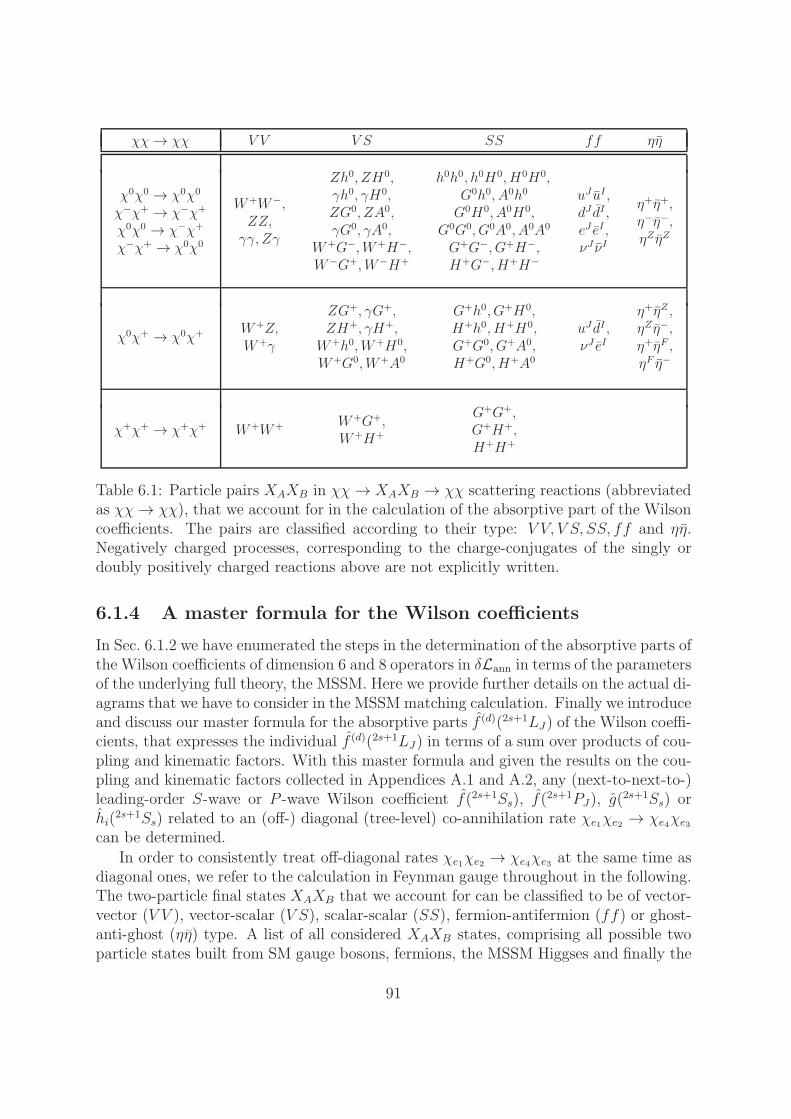
χχ→ χχ V V V S SS ff ηη
χ0χ0 → χ0χ0
χ−χ+ → χ−χ+
χ0χ0 → χ−χ+
χ−χ+ → χ0χ0
W+W−,ZZ,γγ, Zγ
Zh0, ZH0,γh0, γH0,ZG0, ZA0,γG0, γA0,
W+G−,W+H−,W−G+,W−H+
h0h0, h0H0, H0H0,G0h0, A0h0
G0H0, A0H0,G0G0, G0A0, A0A0
G+G−, G+H−,H+G−, H+H−
uJ uI ,dJ dI ,eJ eI ,νJ νI
η+η+,η−η−,ηZ ηZ
χ0χ+ → χ0χ+ W+Z,W+γ
ZG+, γG+,ZH+, γH+,
W+h0,W+H0,W+G0,W+A0
G+h0, G+H0,H+h0, H+H0,G+G0, G+A0,H+G0, H+A0
uJ dI ,νJ eI
η+ηZ ,ηZ η−,η+ηF ,ηF η−
χ+χ+ → χ+χ+ W+W+ W+G+,W+H+
G+G+,G+H+,H+H+
Table 6.1: Particle pairs XAXB in χχ→ XAXB → χχ scattering reactions (abbreviatedas χχ→ χχ), that we account for in the calculation of the absorptive part of the Wilsoncoefficients. The pairs are classified according to their type: V V, V S, SS, ff and ηη.Negatively charged processes, corresponding to the charge-conjugates of the singly ordoubly positively charged reactions above are not explicitly written.
6.1.4 A master formula for the Wilson coefficients
In Sec. 6.1.2 we have enumerated the steps in the determination of the absorptive parts ofthe Wilson coefficients of dimension 6 and 8 operators in δLann in terms of the parametersof the underlying full theory, the MSSM. Here we provide further details on the actual di-agrams that we have to consider in the MSSM matching calculation. Finally we introduceand discuss our master formula for the absorptive parts f (d)(2s+1LJ) of the Wilson coeffi-cients, that expresses the individual f (d)(2s+1LJ ) in terms of a sum over products of cou-pling and kinematic factors. With this master formula and given the results on the cou-pling and kinematic factors collected in Appendices A.1 and A.2, any (next-to-next-to-)leading-order S-wave or P -wave Wilson coefficient f(2s+1Ss), f(
2s+1PJ), g(2s+1Ss) or
hi(2s+1Ss) related to an (off-) diagonal (tree-level) co-annihilation rate χe1χe2 → χe4χe3
can be determined.
In order to consistently treat off-diagonal rates χe1χe2 → χe4χe3 at the same time asdiagonal ones, we refer to the calculation in Feynman gauge throughout in the following.The two-particle final states XAXB that we account for can be classified to be of vector-vector (V V ), vector-scalar (V S), scalar-scalar (SS), fermion-antifermion (ff) or ghost-anti-ghost (ηη) type. A list of all considered XAXB states, comprising all possible twoparticle states built from SM gauge bosons, fermions, the MSSM Higgses and finally the
91
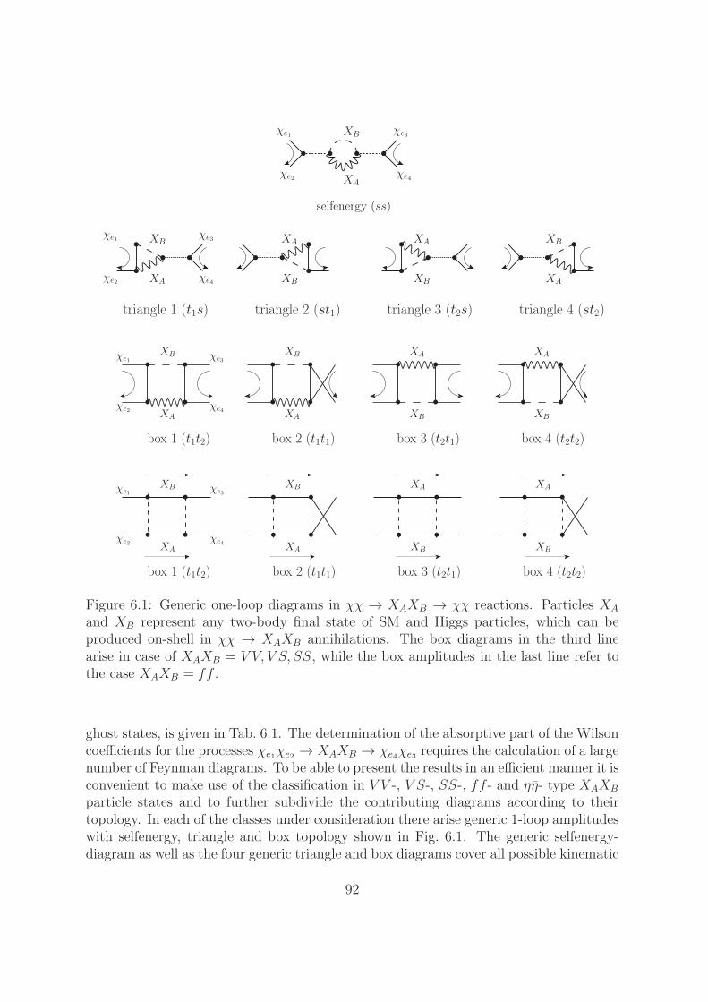
XA
selfenergy (ss)
XBχe1
χe4
χe3
χe2
XA
triangle 1 (t1s)
XB
triangle 3 (t2s) triangle 4 (st2)triangle 2 (st1)
XAXBXB
XBXAXAχe1
χe4
χe3
χe2
XA
box 1 (t1t2)
XB XB XA XA
XA XB
box 3 (t2t1) box 4 (t2t2)box 2 (t1t1)
XB
χe1
χe2
χe3
χe4
XA
box 1 (t1t2)
XB XB XA XA
XA XB
box 3 (t2t1) box 4 (t2t2)box 2 (t1t1)
XB
χe1
χe2
χe3
χe4
Figure 6.1: Generic one-loop diagrams in χχ → XAXB → χχ reactions. Particles XA
and XB represent any two-body final state of SM and Higgs particles, which can beproduced on-shell in χχ → XAXB annihilations. The box diagrams in the third linearise in case of XAXB = V V, V S, SS, while the box amplitudes in the last line refer tothe case XAXB = ff .
ghost states, is given in Tab. 6.1. The determination of the absorptive part of the Wilsoncoefficients for the processes χe1χe2 → XAXB → χe4χe3 requires the calculation of a largenumber of Feynman diagrams. To be able to present the results in an efficient manner it isconvenient to make use of the classification in V V -, V S-, SS-, ff - and ηη- type XAXB
particle states and to further subdivide the contributing diagrams according to theirtopology. In each of the classes under consideration there arise generic 1-loop amplitudeswith selfenergy, triangle and box topology shown in Fig. 6.1. The generic selfenergy-diagram as well as the four generic triangle and box diagrams cover all possible kinematic
92
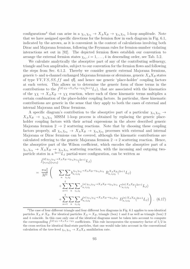
configurations4 that can arise in a χe1χe2 → XAXB → χe4χe3 1-loop amplitude. Notethat we have assigned specific directions for the fermion flow in each diagram in Fig. 6.1,indicated by the arrows, as it is convenient in the context of calculations involving bothDirac and Majorana fermions, following the Feynman rules for fermion-number violatinginteractions set out in [92]. The depicted fermion flows establish our convention toarrange the external fermion states χei , i = 1, . . . , 4 in descending order, see Tab. 5.2.
We calculate analytically the absorptive part of any of the contributing selfenergy,triangle and box amplitudes, subject to our convention for the fermion flows and followingthe steps from Sec. 6.1.2. Thereby we consider generic external Majorana fermions,generic t- and u-channel exchanged Majorana fermions or sfermions, genericXAXB statesof type V V, V S, SS, ff and ηη, and hence use generic ‘place-holder’ coupling factorsat each vertex. This allows us to determine the generic form of those terms in thecontributions to the f (d)χχ→XAXB→χχ(2s+1LJ ), that are associated with the kinematicsof the χχ → XAXB → χχ reaction, where each of these kinematic terms multiplies acertain combination of the place-holder coupling factors. In particular, these kinematiccontributions are generic in the sense that they apply to both the cases of external andinternal Majorana and Dirac fermions.
A specific diagram’s contribution to the absorptive part of a particular χe1χe2 →XAXB → χe4χe3 MSSM 1-loop process is obtained by replacing the generic place-holder coupling factors with their actual expressions in the above described genericMajorana fermion 2 → 2 scattering reactions. Note that by choosing these couplingfactors properly, all χe1χe2 → XAXB → χe4χe3 processes with external and internalMajorana or Dirac fermions can be covered, although the kinematic contributions arecalculated referring to the generic Majorana fermion 2 → 2 scattering reaction. Hence,the absorptive part of the Wilson coefficient, which encodes the absorptive part of aχe1χe2 → XAXB → χe4χe3 scattering reaction, with the incoming and outgoing two-particle states in a 2s+1LJ partial-wave configuration, can be written as
f(d)χe1
χe2→XAXB→χe4
χe3
e1e2e4e3 (2s+1LJ)
=πα2
2
M2
(∑
n
∑
i1,i2
bχe1
χe2→XAXB→χe4
χe3
n, i1i2BXAXB
n, i1i2(2s+1LJ)
+4∑
α=1
∑
n
∑
i1,i2
c(α)χe1
χe2→XAXB→χe4
χe3
n, i1i2C
(α)XAXB
n, i1i2(2s+1LJ )
+
4∑
α=1
∑
n
∑
i1,i2
d(α)χe1
χe2→XAXB→χe4
χe3
n, i1i2D
(α)XAXB
n, i1i2(2s+1LJ)
). (6.17)
4The case of four different triangle and four different box diagrams in Fig. 6.1 applies to non-identicalparticles XA 6= XB. For identical particles XA = XB, triangle (box) 1 and 3 as well as triangle (box) 2and 4 coincide. In this case only one of the identical diagrams must be taken into account to computethe corresponding f (d)χχ→XAXA→χχ coefficients. This rule incorporates the symmetry factor of 1/2 inthe cross section for identical final-state particles, that one would take into account in the conventionalcalculation of the tree-level χe1χe2 → XAXA annihilation rate.
93
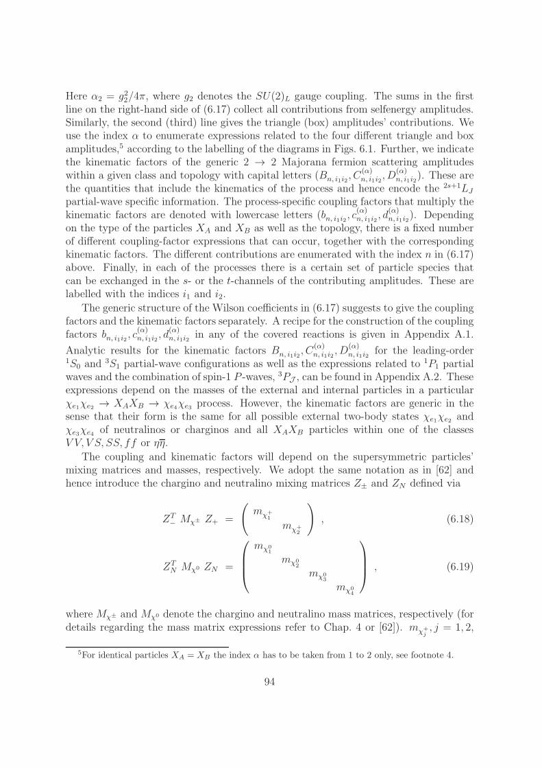
Here α2 = g22/4π, where g2 denotes the SU(2)L gauge coupling. The sums in the firstline on the right-hand side of (6.17) collect all contributions from selfenergy amplitudes.Similarly, the second (third) line gives the triangle (box) amplitudes’ contributions. Weuse the index α to enumerate expressions related to the four different triangle and boxamplitudes,5 according to the labelling of the diagrams in Figs. 6.1. Further, we indicatethe kinematic factors of the generic 2 → 2 Majorana fermion scattering amplitudeswithin a given class and topology with capital letters (Bn, i1i2, C
(α)n, i1i2
, D(α)n, i1i2
). These arethe quantities that include the kinematics of the process and hence encode the 2s+1LJpartial-wave specific information. The process-specific coupling factors that multiply thekinematic factors are denoted with lowercase letters (bn, i1i2, c
(α)n, i1i2
, d(α)n, i1i2
). Dependingon the type of the particles XA and XB as well as the topology, there is a fixed numberof different coupling-factor expressions that can occur, together with the correspondingkinematic factors. The different contributions are enumerated with the index n in (6.17)above. Finally, in each of the processes there is a certain set of particle species thatcan be exchanged in the s- or the t-channels of the contributing amplitudes. These arelabelled with the indices i1 and i2.
The generic structure of the Wilson coefficients in (6.17) suggests to give the couplingfactors and the kinematic factors separately. A recipe for the construction of the couplingfactors bn, i1i2 , c
(α)n, i1i2
, d(α)n, i1i2
in any of the covered reactions is given in Appendix A.1.
Analytic results for the kinematic factors Bn, i1i2, C
(α)n, i1i2
, D(α)n, i1i2
for the leading-order1S0 and 3S1 partial-wave configurations as well as the expressions related to 1P1 partialwaves and the combination of spin-1 P -waves, 3PJ , can be found in Appendix A.2. Theseexpressions depend on the masses of the external and internal particles in a particularχe1χe2 → XAXB → χe4χe3 process. However, the kinematic factors are generic in thesense that their form is the same for all possible external two-body states χe1χe2 andχe3χe4 of neutralinos or charginos and all XAXB particles within one of the classesV V, V S, SS, ff or ηη.
The coupling and kinematic factors will depend on the supersymmetric particles’mixing matrices and masses, respectively. We adopt the same notation as in [62] andhence introduce the chargino and neutralino mixing matrices Z± and ZN defined via
ZT− Mχ± Z+ =
(mχ+
1
mχ+2
), (6.18)
ZTN Mχ0 ZN =
mχ01
mχ02
mχ03
mχ04
, (6.19)
where Mχ± and Mχ0 denote the chargino and neutralino mass matrices, respectively (fordetails regarding the mass matrix expressions refer to Chap. 4 or [62]). mχ+
j, j = 1, 2,
5For identical particles XA = XB the index α has to be taken from 1 to 2 only, see footnote 4.
94
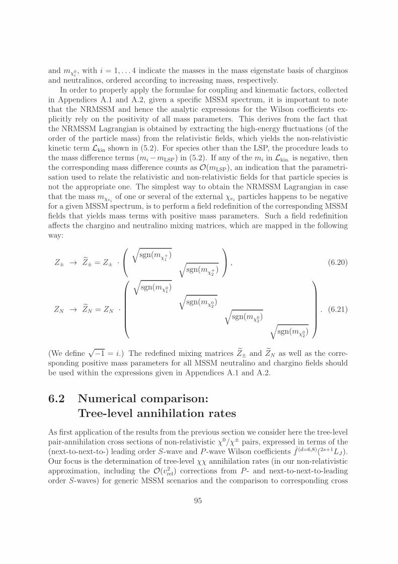
and mχ0i, with i = 1, . . . 4 indicate the masses in the mass eigenstate basis of charginos
and neutralinos, ordered according to increasing mass, respectively.In order to properly apply the formulae for coupling and kinematic factors, collected
in Appendices A.1 and A.2, given a specific MSSM spectrum, it is important to notethat the NRMSSM and hence the analytic expressions for the Wilson coefficients ex-plicitly rely on the positivity of all mass parameters. This derives from the fact thatthe NRMSSM Lagrangian is obtained by extracting the high-energy fluctuations (of theorder of the particle mass) from the relativistic fields, which yields the non-relativistickinetic term Lkin shown in (5.2). For species other than the LSP, the procedure leads tothe mass difference terms (mi−mLSP) in (5.2). If any of the mi in Lkin. is negative, thenthe corresponding mass difference counts as O(mLSP), an indication that the parametri-sation used to relate the relativistic and non-relativistic fields for that particle species isnot the appropriate one. The simplest way to obtain the NRMSSM Lagrangian in casethat the mass mχei
of one or several of the external χei particles happens to be negativefor a given MSSM spectrum, is to perform a field redefinition of the corresponding MSSMfields that yields mass terms with positive mass parameters. Such a field redefinitionaffects the chargino and neutralino mixing matrices, which are mapped in the followingway:
Z± → Z± = Z± ·
√
sgn(mχ+1)√
sgn(mχ+2)
, (6.20)
ZN → ZN = ZN ·
√sgn(mχ0
1)√
sgn(mχ02)√
sgn(mχ02)√sgn(mχ0
2)
. (6.21)
(We define√−1 = i.) The redefined mixing matrices Z± and ZN as well as the corre-
sponding positive mass parameters for all MSSM neutralino and chargino fields shouldbe used within the expressions given in Appendices A.1 and A.2.
6.2 Numerical comparison:
Tree-level annihilation rates
As first application of the results from the previous section we consider here the tree-levelpair-annihilation cross sections of non-relativistic χ0/χ± pairs, expressed in terms of the(next-to-next-to-) leading order S-wave and P -wave Wilson coefficients f (d=6,8)(2s+1LJ).Our focus is the determination of tree-level χχ annihilation rates (in our non-relativisticapproximation, including the O(v2rel) corrections from P - and next-to-next-to-leadingorder S-waves) for generic MSSM scenarios and the comparison to corresponding cross
95
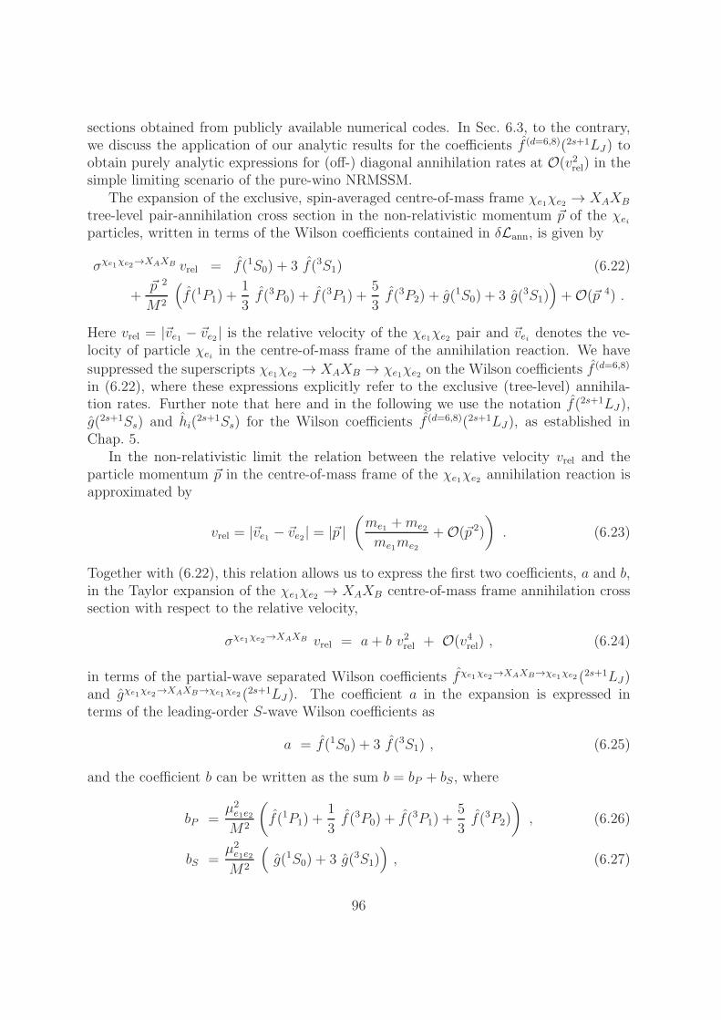
sections obtained from publicly available numerical codes. In Sec. 6.3, to the contrary,we discuss the application of our analytic results for the coefficients f (d=6,8)(2s+1LJ ) toobtain purely analytic expressions for (off-) diagonal annihilation rates at O(v2rel) in thesimple limiting scenario of the pure-wino NRMSSM.
The expansion of the exclusive, spin-averaged centre-of-mass frame χe1χe2 → XAXB
tree-level pair-annihilation cross section in the non-relativistic momentum ~p of the χeiparticles, written in terms of the Wilson coefficients contained in δLann, is given by
σχe1χe2
→XAXB vrel = f(1S0) + 3 f(3S1) (6.22)
+~p 2
M2
(f(1P1) +
1
3f(3P0) + f(3P1) +
5
3f(3P2) + g(1S0) + 3 g(3S1)
)+O(~p 4) .
Here vrel = |~ve1 − ~ve2 | is the relative velocity of the χe1χe2 pair and ~vei denotes the ve-locity of particle χei in the centre-of-mass frame of the annihilation reaction. We have
suppressed the superscripts χe1χe2 → XAXB → χe1χe2 on the Wilson coefficients f (d=6,8)
in (6.22), where these expressions explicitly refer to the exclusive (tree-level) annihila-tion rates. Further note that here and in the following we use the notation f(2s+1LJ),g(2s+1Ss) and hi(
2s+1Ss) for the Wilson coefficients f (d=6,8)(2s+1LJ ), as established inChap. 5.
In the non-relativistic limit the relation between the relative velocity vrel and theparticle momentum ~p in the centre-of-mass frame of the χe1χe2 annihilation reaction isapproximated by
vrel = |~ve1 − ~ve2 | = |~p |(me1 +me2
me1me2
+O(~p 2)
). (6.23)
Together with (6.22), this relation allows us to express the first two coefficients, a and b,in the Taylor expansion of the χe1χe2 → XAXB centre-of-mass frame annihilation crosssection with respect to the relative velocity,
σχe1χe2
→XAXB vrel = a+ b v2rel + O(v4rel) , (6.24)
in terms of the partial-wave separated Wilson coefficients fχe1χe2
→XAXB→χe1χe2 (2s+1LJ)
and gχe1χe2
→XAXB→χe1χe2 (2s+1LJ). The coefficient a in the expansion is expressed in
terms of the leading-order S-wave Wilson coefficients as
a = f(1S0) + 3 f(3S1) , (6.25)
and the coefficient b can be written as the sum b = bP + bS, where
bP =µ2e1e2
M2
(f(1P1) +
1
3f(3P0) + f(3P1) +
5
3f(3P2)
), (6.26)
bS =µ2e1e2
M2
(g(1S0) + 3 g(3S1)
), (6.27)
96
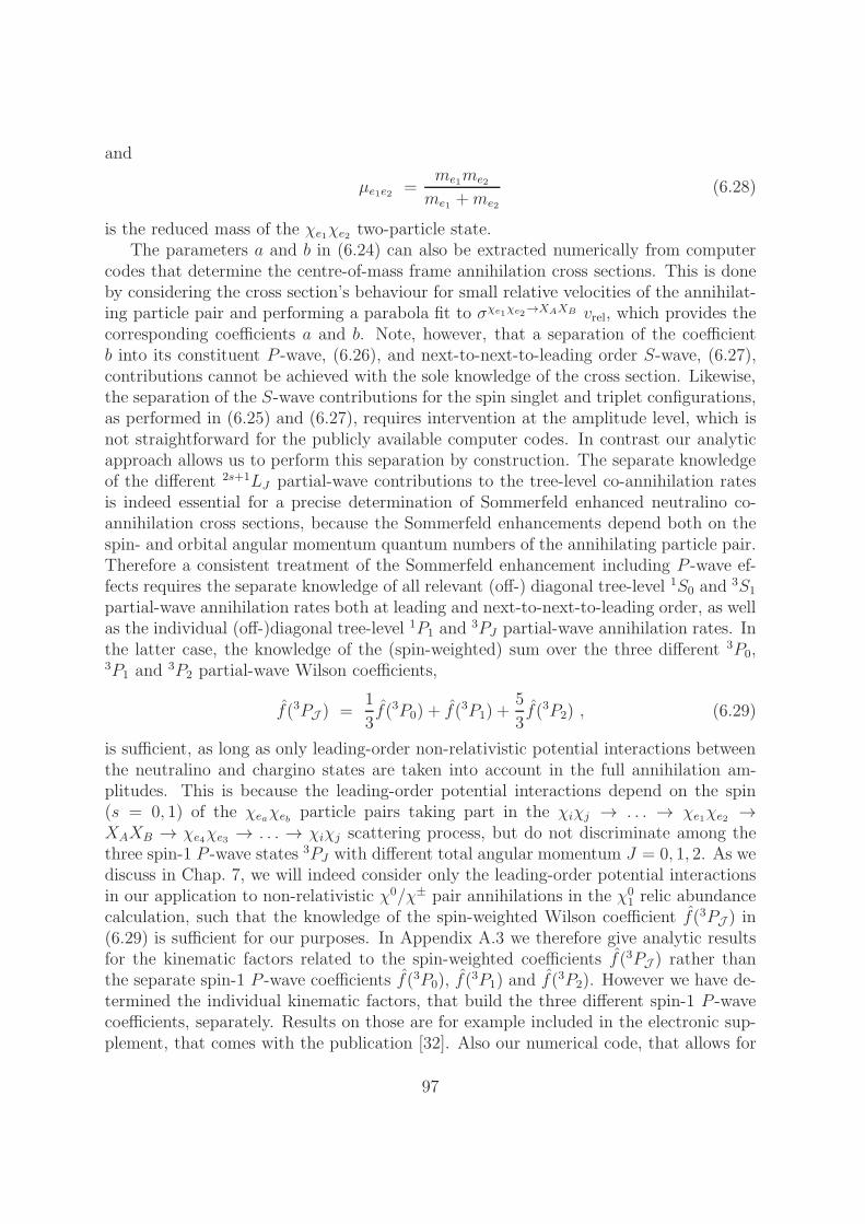
and
µe1e2 =me1me2
me1 +me2
(6.28)
is the reduced mass of the χe1χe2 two-particle state.The parameters a and b in (6.24) can also be extracted numerically from computer
codes that determine the centre-of-mass frame annihilation cross sections. This is doneby considering the cross section’s behaviour for small relative velocities of the annihilat-ing particle pair and performing a parabola fit to σχe1
χe2→XAXB vrel, which provides the
corresponding coefficients a and b. Note, however, that a separation of the coefficientb into its constituent P -wave, (6.26), and next-to-next-to-leading order S-wave, (6.27),contributions cannot be achieved with the sole knowledge of the cross section. Likewise,the separation of the S-wave contributions for the spin singlet and triplet configurations,as performed in (6.25) and (6.27), requires intervention at the amplitude level, which isnot straightforward for the publicly available computer codes. In contrast our analyticapproach allows us to perform this separation by construction. The separate knowledgeof the different 2s+1LJ partial-wave contributions to the tree-level co-annihilation ratesis indeed essential for a precise determination of Sommerfeld enhanced neutralino co-annihilation cross sections, because the Sommerfeld enhancements depend both on thespin- and orbital angular momentum quantum numbers of the annihilating particle pair.Therefore a consistent treatment of the Sommerfeld enhancement including P -wave ef-fects requires the separate knowledge of all relevant (off-) diagonal tree-level 1S0 and
3S1
partial-wave annihilation rates both at leading and next-to-next-to-leading order, as wellas the individual (off-)diagonal tree-level 1P1 and
3PJ partial-wave annihilation rates. Inthe latter case, the knowledge of the (spin-weighted) sum over the three different 3P0,3P1 and 3P2 partial-wave Wilson coefficients,
f(3PJ ) =1
3f(3P0) + f(3P1) +
5
3f(3P2) , (6.29)
is sufficient, as long as only leading-order non-relativistic potential interactions betweenthe neutralino and chargino states are taken into account in the full annihilation am-plitudes. This is because the leading-order potential interactions depend on the spin(s = 0, 1) of the χeaχeb particle pairs taking part in the χiχj → . . . → χe1χe2 →XAXB → χe4χe3 → . . . → χiχj scattering process, but do not discriminate among thethree spin-1 P -wave states 3PJ with different total angular momentum J = 0, 1, 2. As wediscuss in Chap. 7, we will indeed consider only the leading-order potential interactionsin our application to non-relativistic χ0/χ± pair annihilations in the χ0
1 relic abundancecalculation, such that the knowledge of the spin-weighted Wilson coefficient f(3PJ ) in(6.29) is sufficient for our purposes. In Appendix A.3 we therefore give analytic resultsfor the kinematic factors related to the spin-weighted coefficients f(3PJ ) rather thanthe separate spin-1 P -wave coefficients f(3P0), f(
3P1) and f(3P2). However we have de-
termined the individual kinematic factors, that build the three different spin-1 P -wavecoefficients, separately. Results on those are for example included in the electronic sup-plement, that comes with the publication [32]. Also our numerical code, that allows for
97

the determination of the (off-) diagonal short-distance annihilation rates in χ0/χ± pairannihilations and that has been developed as part of this work, contains separate resultsfor the spin-1 P -wave Wilson coefficients f(3P0,1,2).
Recently, Sommerfeld corrections including P -wave effects have been subject of studyat 1-loop [93] and with full resummation [94]. In these studies, the next-to-next-to-leading order contributions in the expansion of the relevant (co-)annihilation rates wereassumed to be given only by P -waves. While such reasoning is justified when the leading-order S-wave contributions to the annihilation rates are strongly suppressed with respectto the next-to-next-to-leading order coefficients in (6.24), it does not hold for the generalcase. In particular, P - and next-to-next-to-leading order S-wave terms can come withdiffering signs, such that a partial compensation of different next-to-next-to-leading ordercontributions to the annihilation rates may occur. We illustrate this effect in Sec. 6.2.1.
We have performed a dedicated numeric check of our results for the non-relativisticallyapproximated χe1χe2 → XAXB tree-level annihilation cross sections as given in (6.22,6.24) for all initial state two-particle pairs in Tab. 5.1 into all accessible SM and Higgstwo-particle final states. To this end several MSSM spectra have been considered, whichwe compute using the spectrum calculator SuSpect [86] and its implementation of thephenomenological MSSM, a model with 27 free parameters. For each spectrum, we ob-tain the coefficients a and b in (6.25) and (6.26, 6.27) from our analytic calculation, andcompare them with the corresponding coefficients extracted purely numerically usingMadGraph [89] to calculate the cross sections. Our results for the coefficient a agreewith the corresponding numeric expression extracted from MadGraph data at per millevel. Similarly, we find agreement of the coefficients b derived with (6.26, 6.27) andextracted from MadGraph data at 1% up to per mil level, where the level of agree-ment slightly varies depending on the initial- and final-state particles. In addition, thelevel of agreement on the parameter b depends on the interval of the vrel variable usedfor the parabola fit to the MadGraph data, which for the numbers quoted above istaken as vrel/c = [0, 0.4]. We find that the non-relativistic approximation is reliablefor single-particle velocities up to vei/c ∼ 0.3. For such velocities the absolute errorof the non-relativistic approximation to σχe1
χe2→XAXB vrel with respect to the unex-
panded σχe1χe2
→XAXB vrel expression lies within the level of a few percent. Therefore thenon-relativistic approximation has an acceptable accuracy for calculations in the earlyUniverse during the time of χei-decoupling, as the mean velocity of the χei in that periodwas around vei/c ∼ 0.2.
In the following subsections we give several examples for the numerical comparisonwith MadGraph. In addition we discuss in detail the impact of the different partial-wave contributions on the corresponding annihilation cross section times relative velocity,σχe1
χe2→XAXB vrel, as obtained from our results. To this end we have selected processes
with significantly different S- and P -wave dependence. The SuSpect-generated MSSMspectrum, that underlies all results presented in the next sections, contains a wino-likeneutralino LSP with mass mχ0
1= 2748.92GeV, and an almost mass-degenerate wino-like
chargino partner with mχ+1= 2749.13GeV.
98
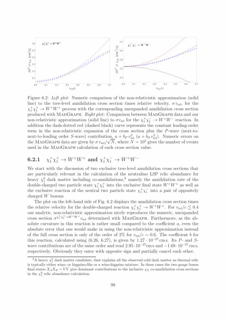
0.0 0.1 0.2 0.3 0.4 0.5 0.6 0.7
5.1
5.2
5.3
5.4
5.5
5.6
vrelc
1027Σ
v rel@c
m3
sD
Χ1+Χ1+ ®W+W+
0.0 0.1 0.2 0.3 0.4 0.5 0.6 0.7
2.4
2.6
2.8
3.0
3.2
vrel c
1027Σ
v rel@c
m3sD Χ1
+Χ1-® W +W -
Figure 6.2: Left plot: Numeric comparison of the non-relativistic approximation (solidline) to the tree-level annihilation cross section times relative velocity, σ vrel, for theχ+1 χ
+1 →W+W+ process with the corresponding unexpanded annihilation cross section
produced withMadGraph. Right plot: Comparison between MadGraph data and ournon-relativistic approximation (solid line) to σvrel for the χ
+1 χ
−1 → W+W− reaction. In
addition the dash-dotted red (dashed black) curve represents the constant leading-orderterm in the non-relativistic expansion of the cross section plus the P -wave (next-to-next-to-leading order S-wave) contribution, a + bP v
2rel (a + bS v
2rel). Numeric errors on
the MadGraph data are given by σ vrel/√N , where N = 105 gives the number of events
used in the MadGraph calculation of each cross section value.
6.2.1 χ+1 χ
+1 → W+W+ and χ+
1 χ−1 → W+W−
We start with the discussion of two exclusive tree-level annihilation cross sections thatare particularly relevant in the calculation of the neutralino LSP relic abundance forheavy χ0
1 dark matter including co-annihilations,6 namely the annihilation rate of thedouble-charged two particle state χ+
1 χ+1 into the exclusive final state W+W+ as well as
the exclusive reaction of the neutral two particle state χ+1 χ
−1 into a pair of oppositely
charged W bosons.The plot on the left-hand side of Fig. 6.2 displays the annihilation cross section times
the relative velocity for the double-charged reaction χ+1 χ
+1 → W+W+. For vrel/c . 0.4
our analytic, non-relativistic approximation nicely reproduces the numeric, unexpandedcross section σχ
+1 χ
+1 →W+W+
vrel determined with MadGraph. Furthermore, as the ab-solute curvature in this reaction is rather small compared to the coefficient a, even theabsolute error that one would make in using the non-relativistic approximation insteadof the full cross section is only of the order of 2% for vrel/c ∼ 0.6. The coefficient b forthis reaction, calculated using (6.26, 6.27), is given by 1.27 · 10−27 cm s. Its P - and S-wave contributions are of the same order and read 2.95 ·10−27cm s and −1.68 ·10−27 cm s,respectively. Obviously they enter with opposite sign and partially cancel each other.
6A heavy χ01 dark matter candidate, that explains all the observed cold dark matter as thermal relic
is typically either wino- or higgsino-like or a wino-higgsino mixture. In these cases the two gauge bosonfinal states XAXB = V V give dominant contributions to the inclusive χχ co-annihilation cross sectionsin the χ0
1 relic abundance calculation.
99
Such partial compensation of the P - and next-to-next-to-leading order S-wave contri-butions to the cross section can be seen explicitly in the right hand side plot in Fig. 6.2.The plot displays the χ+
1 χ−1 → W+W− tree-level annihilation rate, where the solid
blue line corresponds to the non-relativistic approximation to the tree-level annihila-tion cross section, σχ
+1 χ
−
1 →W+W−
vrel, and the points correspond to the full tree-levelresult obtained with MadGraph. The deviation between our approximation and theMadGraph data is at one percent level for vrel/c ∼ 0.6 and in the per mil regimefor smaller relative velocities. In addition the composition of the non-relativistic ap-proximation to σχ
+1 χ
−
1 →W+W−
vrel out of P - and next-to-next-to-leading order S-wavecontributions can be directly read off from Fig. 6.2: the dash-dotted red line repre-sents the contribution a + bP v2rel to (6.24), while the dashed black line is a + bS v2rel.While both bP and bS are roughly of the same order of magnitude, the summed P -wave contributions enter with a positive sign (bP c
2 = 1.86 · 10−27 cm3 s−1), whereas thesummed next-to-next-to-leading order S-wave contributions come with a negative weight,bS c
2 = −0.88 · 10−27 cm3 s−1. It is worth noting that the sum of next-to-next-to-leadingorder corrections in the χ+
1 χ−1 → W+W− tree-level cross section times relative velocity
gives a ∼ 6% correction to the leading-order approximation for vrel/c ∼ 0.4. For thisrelative velocity, the corrections to the leading-order approximation from P -waves onlyamount to ∼ 11%, while those from next-to-next-to-leading order S-wave contributionsamount to ∼ −5%. Hence, in the light of the expected future experimental precision onthe measured dark matter density, it is crucial to take these corrections into account.Further, as generically the Sommerfeld enhancements for each of the contributing par-tial waves are different, we consistently consider the Sommerfeld enhancements on thedifferent partial-wave contributions to the cross sections separately.
The fact that the P -wave terms in the two examples of Fig. 6.2 contribute with pos-itive sign is generic: the sum of all 2s+1PJ partial-wave contributions to any χe1χe2 →XAXB annihilation cross section has to be positive, as it results from the absolute squareof the coefficient of theO(p) terms in the expansion of the annihilation amplitude. More-over, the separate 2s+1PJ partial-wave contributions must also be positive, since different2s+1PJ -wave amplitudes do not interfere in the absolute square of the annihilation am-plitude due to total angular-momentum conservation and the additional conservation ofspin in the non-relativistic regime. The next-to-next-to-leading order S-wave contribu-tions to the χe1χe2 → XAXB annihilation cross section, however, result from the productof leading-order and next-to-next-to-leading order S-wave contributions in the expansionof the χe1χe2 → XAXB amplitude. There is a priori no reason why this product shouldbe positive, and hence negative next-to-next-to-leading order S-wave contributions tothe cross section can occur, as can be explicitly seen in the examples presented in thissection.
6.2.2 The S-wave dominated processes χ01χ
+1 → tb, ud
We continue with the discussion of χ01χ
+1 annihilation reactions into exclusive final states
built from a pair of fermions. The plot on the left-hand side in Fig. 6.3 depicts the
100
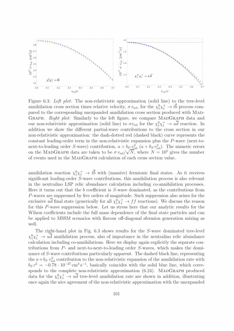
0.0 0.1 0.2 0.3 0.4 0.5 0.6 0.7
3.2
3.3
3.4
3.5
3.6
3.7
3.8
vrelc
1027Σ
v rel@c
m3
sD
Χ10Χ1+ ® tb
0.0 0.1 0.2 0.3 0.4 0.5 0.6 0.7
1.3
1.4
1.5
1.6
vrel c
1027Σ
v rel@c
m3sD
Χ10Χ1+® u d
Figure 6.3: Left plot: The non-relativistic approximation (solid line) to the tree-levelannihilation cross section times relative velocity, σ vrel, for the χ
01χ
+1 → tb process com-
pared to the corresponding unexpanded annihilation cross section produced with Mad-
Graph. Right plot: Similarly to the left figure, we compare MadGraph data andour non-relativistic approximation (solid line) to σvrel for the χ0
1χ+1 → ud reaction. In
addition we show the different partial-wave contributions to the cross section in ournon-relativistic approximation: the dash-dotted red (dashed black) curve represents theconstant leading-order term in the non-relativistic expansion plus the P -wave (next-to-next-to-leading order S-wave) contribution, a + bP v
2rel (a + bS v
2rel). The numeric errors
on the MadGraph data are taken to be σ vrel/√N , where N = 105 gives the number
of events used in the MadGraph calculation of each cross section value.
annihilation reaction χ01χ
+1 → tb with (massive) fermionic final states. As it receives
significant leading-order S-wave contributions, this annihilation process is also relevantin the neutralino LSP relic abundance calculation including co-annihilation processes.Here it turns out that the b coefficient is S-wave dominated, as the contributions fromP -waves are suppressed by five orders of magnitude. Such suppression also arises for theexclusive ud final state (generically for all χ0
1χ+1 → ff reactions). We discuss the reason
for this P -wave suppression below. Let us stress here that our analytic results for theWilson coefficients include the full mass dependence of the final state particles and canbe applied to MSSM scenarios with flavour off-diagonal sfermion generation mixing aswell.
The right-hand plot in Fig. 6.3 shows results for the S-wave dominated tree-levelχ01χ
+1 → ud annihilation process, also of importance in the neutralino relic abundance
calculation including co-annihilations. Here we display again explicitly the separate con-tributions from P - and next-to-next-to-leading order S-waves, which makes the domi-nance of S-wave contributions particularly apparent. The dashed black line, representingthe a+ bS v
2rel contribution to the non-relativistic expansion of the annihilation rate with
bS c2 = −0.78 · 10−27 cm3 s−1, basically coincides with the solid blue line, which corre-
sponds to the complete non-relativistic approximation (6.24). MadGraph produceddata for the χ0
1χ+1 → ud tree-level annihilation rate are shown in addition, illustrating
once again the nice agreement of the non-relativistic approximation with the unexpanded
101
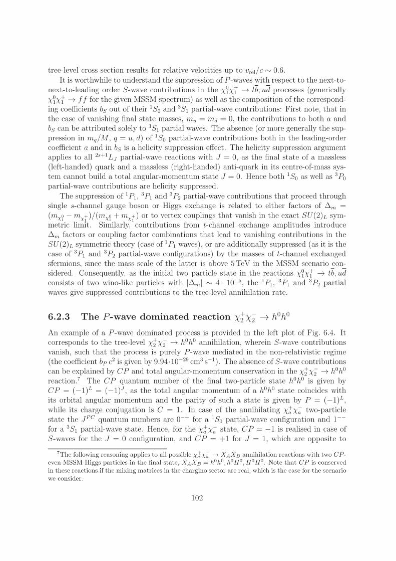
tree-level cross section results for relative velocities up to vrel/c ∼ 0.6.It is worthwhile to understand the suppression of P -waves with respect to the next-to-
next-to-leading order S-wave contributions in the χ01χ
+1 → tb, ud processes (generically
χ01χ
+1 → ff for the given MSSM spectrum) as well as the composition of the correspond-
ing coefficients bS out of their 1S0 and3S1 partial-wave contributions: First note, that in
the case of vanishing final state masses, mu = md = 0, the contributions to both a andbS can be attributed solely to 3S1 partial waves. The absence (or more generally the sup-pression in mq/M , q = u, d) of 1S0 partial-wave contributions both in the leading-ordercoefficient a and in bS is a helicity suppression effect. The helicity suppression argumentapplies to all 2s+1LJ partial-wave reactions with J = 0, as the final state of a massless(left-handed) quark and a massless (right-handed) anti-quark in its centre-of-mass sys-tem cannot build a total angular-momentum state J = 0. Hence both 1S0 as well as
3P0
partial-wave contributions are helicity suppressed.The suppression of 1P1,
3P1 and3P2 partial-wave contributions that proceed through
single s-channel gauge boson or Higgs exchange is related to either factors of ∆m =(mχ0
1−mχ+
1)/(mχ0
1+mχ+
1) or to vertex couplings that vanish in the exact SU(2)L sym-
metric limit. Similarly, contributions from t-channel exchange amplitudes introduce∆m factors or coupling factor combinations that lead to vanishing contributions in theSU(2)L symmetric theory (case of 1P1 waves), or are additionally suppressed (as it is thecase of 3P1 and 3P2 partial-wave configurations) by the masses of t-channel exchangedsfermions, since the mass scale of the latter is above 5TeV in the MSSM scenario con-sidered. Consequently, as the initial two particle state in the reactions χ0
1χ+1 → tb, ud
consists of two wino-like particles with |∆m| ∼ 4 · 10−5, the 1P1,3P1 and 3P2 partial
waves give suppressed contributions to the tree-level annihilation rate.
6.2.3 The P -wave dominated reaction χ+2 χ−2 → h0h0
An example of a P -wave dominated process is provided in the left plot of Fig. 6.4. Itcorresponds to the tree-level χ+
2 χ−2 → h0h0 annihilation, wherein S-wave contributions
vanish, such that the process is purely P -wave mediated in the non-relativistic regime(the coefficient bP c
2 is given by 9.94·10−29 cm3 s−1). The absence of S-wave contributionscan be explained by CP and total angular-momentum conservation in the χ+
2 χ−2 → h0h0
reaction.7 The CP quantum number of the final two-particle state h0h0 is given byCP = (−1)L = (−1)J , as the total angular momentum of a h0h0 state coincides withits orbital angular momentum and the parity of such a state is given by P = (−1)L,while its charge conjugation is C = 1. In case of the annihilating χ+
a χ−a two-particle
state the JPC quantum numbers are 0−+ for a 1S0 partial-wave configuration and 1−−
for a 3S1 partial-wave state. Hence, for the χ+a χ
−a state, CP = −1 is realised in case of
S-waves for the J = 0 configuration, and CP = +1 for J = 1, which are opposite to
7The following reasoning applies to all possible χ+a χ
−a → XAXB annihilation reactions with two CP -
even MSSM Higgs particles in the final state, XAXB = h0h0, h0H0, H0H0. Note that CP is conservedin these reactions if the mixing matrices in the chargino sector are real, which is the case for the scenariowe consider.
102
0.0 0.1 0.2 0.3 0.4 0.5 0.6 0.7
0
1000
2000
3000
4000
vrel c
1032Σ
v rel@c
m3sD Χ2
+Χ2-® h 0 h 0
0.0 0.1 0.2 0.3 0.4 0.5 0.6 0.7
1.1
1.2
1.3
1.4
vrelHin Lc
1027GΧΧ®
WW®ΧΧ@c
m3sD
Χ1+Χ1-®W +W -
® Χ2+Χ2-
Figure 6.4: Left plot: Numeric comparison of the non-relativistic approximation (solidblue curve) to the tree-level annihilation cross section times relative velocity, σ vrel, for theP -wave dominated χ+
2 χ−2 → h0h0 reaction to data for the corresponding unexpanded an-
nihilation cross section produced with MadGraph. Numeric errors on the MadGraph
data are taken to be σ vrel/√N , where N = 105 gives the number of events used in the
MadGraph calculation of each cross section value. The dash-dotted red and dashedblack lines represent the constant leading-order term plus the P -wave or the next-to-next-to-leading order S-wave contribution, a + bP v
2rel or a + bS v
2rel, respectively. Note
that the a+bP v2rel contribution and the non-relativistic approximation coincide, as there
are no S-wave contributions in this particular annihilation reaction. Right plot: Off-diagonal annihilation rate Γ for the reaction χ+
1 χ−1 → W+W− → χ+
2 χ−2 . The solid line
includes all contributions to Γ up to next-to-next-to-leading order in the non-relativisticexpansion. It is obtained from (6.30) assuming that p and p′ are parallel to each other.The constant dotted blue line gives the leading-order approximation to Γ. Summing theP - or the (momentum-dependent) next-to-next-to-leading order S-wave contributions tothe constant S-wave terms (given by the leading order plus the terms proportional to δmand δm) yields the dash-dotted red or the dashed black line, respectively. The curves
are plotted against the relative velocity v(in)rel of the incoming state χ+
1 χ−1 .
the CP quantum numbers of a h0h0 final state with the same total angular momentum.The same reasoning explains the absence of 3P1 annihilations in any of the processesχ+a χ
−a → XAXB with XAXB = h0h0, h0H0, H0H0, as the JPC quantum numbers of the
3P1 partial-wave configuration of the incoming χ+a χ
−a states are 1++, hence CP = +1 for
J = 1. This is opposite to the CP quantum number of the two CP -even Higgs bosonfinal state with total angular momentum J = 1.
Let us finally note that there are also no contributions from 1P1 partial waves in theprocess shown in the left plot in Fig. 6.4. This feature is generic to χ+
a χ−b → XAXB
annihilations with identical scalar particles in the final state, XAXB = h0h0, H0H0.The argument relies on the statistics of the final state identical bosons, and appliesto all χ+
a χ−b incoming states and not only to particle-anti-particle states χ+
a χ−a : Bose
statistics forbids the two identical final state scalars to be in a J = L = 1 state, as thecorresponding two-particle wave-function for odd total angular momentum J would be
103
anti-symmetric. This argument can also be used to explain the absence of the J = 1 3S1
and 3P1 states in a χ+a χ
−b → h0h0, H0H0 annihilation reaction.
Generically, if the coefficient a in the expansion (6.24) is suppressed with respect tothe coefficient b, the curvature and hence the corresponding non-relativistic annihilationprocess is P -wave dominated. This property derives from the fact, that the leading-order coefficient a is related to the product of the leading-order S-wave contributionsto the tree-level annihilation amplitude with its complex conjugate. As the next-to-next-to-leading order S-wave contributions to the coefficient b result from the product ofleading-order with next-to-next-to-leading order S-wave contributions in the annihilationamplitudes, a suppressed coefficient a indicates a small next-to-next-to-leading order S-wave contribution to the coefficient b as well.
6.2.4 The off-diagonal χ+1 χ−1 →W+W− → χ+
2 χ−2 rate
In order to discuss the importance of the non-relativistic corrections to not only the crosssections but also the off-diagonal annihilation rates, we generalise the definition of theannihilation rates to include off-diagonal reactions. We define the centre-of-mass frametree-level annihilation rate Γ associated with the (off-) diagonal χe1χe2 → XAXB →χe4χe3 scattering reaction as the product of the χe1χe2 → XAXB tree-level annihilationamplitude with the complex conjugate of the tree-level amplitude for the χe4χe3 →XAXB annihilation reaction, integrated over the final XAXB particles’ phase space8 andaveraged over the spin states of the respective incoming particles χei, i = 1, . . . , 4. In thelatter spin-average it is assumed that the χe1χe2 and χe4χe3 pair reside in the same spinstate.9 The external χeaχeb states are further taken to be non-relativistic normalisedin order to match with the definition of the annihilation cross section times relativevelocity in case of diagonal reactions χe1χe2 → XAXB → χe1χe2. In terms of the Wilsoncoefficients of the four-fermion operators, the expansion of the annihilation rate Γ in thenon-relativistic momenta and in the mass differences δm, δm, is then given by
Γχe1χe2
→XAXB→χe4χe3 = f(1S0) + 3 f(3S1) (6.30)
+δm
M
(h1(
1S0) + 3 h1(3S1)
)+δm
M
(h2(
1S0) + 3 h2(3S1)
)
+p · p ′
M2
(f(1P1) +
1
3f(3P0) + f(3P1) +
5
3f(3P2)
)
8 The product of tree-level annihilation amplitudes has to be multiplied with an additional symmetryfactor of 1/2 if the final state particles are identical, XA = XB.
9In the calculation of Sommerfeld enhanced χiχj → XAXB pair-annihilation rates through the imag-inary part of the χiχj → . . . → χe1χe2 → XAXB → χe4χe3 → . . . → χiχj forward scattering reaction,the assumption that the incoming and outgoing particle pairs in the χe1χe2 → XAXB → χe4χe3 short-distance annihilation part have the same spin state implies that just leading-order potential interactionsin the χiχj → . . . → χe1χe2 and χiχj → . . . → χe4χe3 scattering reactions are considered, since thelong-range potentials are spin-diagonal only at leading order and hence pass the spin-configuration ofthe incoming χiχj pair to the χe1χe2 and χe4χe3 pairs. Note that we restrict to the case of leading-orderpotential interactions in this work, see Sec. 7.
104
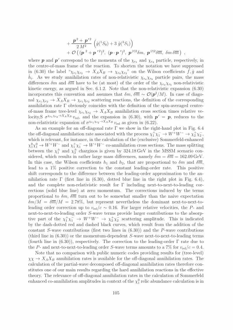
+p 2 + p ′ 2
2M2
(g(1S0) + 3 g(3S1)
)
+ O((p 2 + p ′ 2)2, (p · p ′)2, p (′)2δm, p (′)2δm, δm δm
),
where p and p ′ correspond to the momenta of the χe1 and χe4 particle, respectively, inthe centre-of-mass frame of the reaction. To shorten the notation we have suppressedin (6.30) the label “χe1χe2 → XAXB → χe4χe3” on the Wilson coefficients f , g andhi. As we study annihilation rates of non-relativistic χeaχeb particle pairs, the massdifferences δm and δm have to be (at most) of the order of the χeaχeb non-relativistickinetic energy, as argued in Sec. 6.1.2. Note that the non-relativistic expansion (6.30)incorporates this convention and assumes that δm, δm ∼ O(p2/M). In case of diago-nal χe1χe2 → XAXB → χe1χe2 scattering reactions, the definition of the correspondingannihilation rate Γ obviously coincides with the definition of the spin-averaged centre-of-mass frame tree-level χe1χe2 → XAXB annihilation cross section times relative ve-locity,S σχe1
χe2→XAXB vrel, and the expansion in (6.30), with p ′ = p, reduces to the
non-relativistic expansion of σχe1χe2
→XAXB vrel as given in (6.22).As an example for an off-diagonal rate Γ we show in the right-hand plot in Fig. 6.4
the off-diagonal annihilation rate associated with the process χ+1 χ
−1 → W+W− → χ+
2 χ−2 ,
which is relevant, for instance, in the calculation of the (exclusive) Sommerfeld-enhancedχ01χ
01 →W+W− and χ+
1 χ−1 → W+W− co-annihilation cross sections. The mass splitting
between the χ±1 and χ±
2 charginos is given by 324.18GeV in the MSSM scenario con-sidered, which results in rather large mass differences, namely δm = δm = 162.09GeV.In this case, the Wilson coefficients h1 and h2, that are proportional to δm and δm,lead to a 1% positive correction to the constant leading-order rate. This positiveshift corresponds to the difference between the leading-order approximation to the an-nihilation rate Γ (first line in (6.30), dotted blue line in the right plot in Fig. 6.4),and the complete non-relativistic result for Γ including next-to-next-to-leading cor-rections (solid blue line) at zero momentum. The corrections induced by the termsproportional to δm, δm turn out to be somewhat smaller than the naive expectationδm/M = δm/M = 2.78%, but represent nevertheless the dominant next-to-next-to-leading order correction up to vrel/c ∼ 0.16. For larger relative velocities, the P - andnext-to-next-to-leading order S-wave terms provide larger contributions to the absorp-tive part of the χ+
1 χ−1 → W+W− → χ+
2 χ−2 scattering amplitude. This is indicated
by the dash-dotted red and dashed black curves, which result from the addition of theconstant S-wave contributions (first two lines in (6.30)) and the P -wave contributions(third line in (6.30)) or the momentum-dependent S-wave next-to-next-to-leading terms(fourth line in (6.30)), respectively. The correction to the leading-order Γ rate due tothe P - and next-to-next-to-leading order S-wave terms amounts to a 7% for vrel/c = 0.4.
Note that no comparison with public numeric codes providing results for (tree-level)χχ → XAXB annihilation rates is available for the off-diagonal annihilation rates. Thecalculation of the partial-wave decomposed off-diagonal annihilation rates therefore con-stitutes one of our main results regarding the hard annihilation reactions in the effectivetheory. The relevance of off-diagonal annihilation rates in the calculation of Sommerfeldenhanced co-annihilation amplitudes in context of the χ0
1 relic abundance calculation is in
105
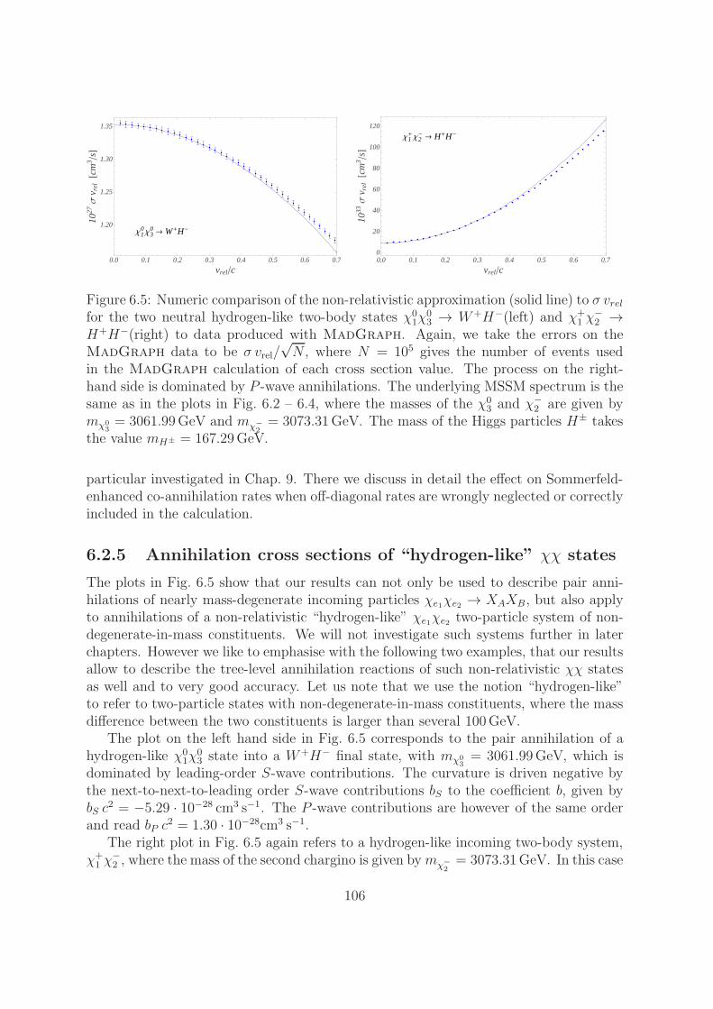
0.0 0.1 0.2 0.3 0.4 0.5 0.6 0.7
1.20
1.25
1.30
1.35
vrelc
1027Σ
v rel@c
m3
sD
Χ10Χ3
0 ®W+H-
0.0 0.1 0.2 0.3 0.4 0.5 0.6 0.70
20
40
60
80
100
120
vrelc
1033Σ
v rel@c
m3
sD
Χ1+Χ2- ® H+H-
Figure 6.5: Numeric comparison of the non-relativistic approximation (solid line) to σ vrelfor the two neutral hydrogen-like two-body states χ0
1χ03 → W+H−(left) and χ+
1 χ−2 →
H+H−(right) to data produced with MadGraph. Again, we take the errors on theMadGraph data to be σ vrel/
√N , where N = 105 gives the number of events used
in the MadGraph calculation of each cross section value. The process on the right-hand side is dominated by P -wave annihilations. The underlying MSSM spectrum is thesame as in the plots in Fig. 6.2 – 6.4, where the masses of the χ0
3 and χ−2 are given by
mχ03= 3061.99GeV and mχ−
2= 3073.31GeV. The mass of the Higgs particles H± takes
the value mH± = 167.29GeV.
particular investigated in Chap. 9. There we discuss in detail the effect on Sommerfeld-enhanced co-annihilation rates when off-diagonal rates are wrongly neglected or correctlyincluded in the calculation.
6.2.5 Annihilation cross sections of “hydrogen-like” χχ states
The plots in Fig. 6.5 show that our results can not only be used to describe pair anni-hilations of nearly mass-degenerate incoming particles χe1χe2 → XAXB, but also applyto annihilations of a non-relativistic “hydrogen-like” χe1χe2 two-particle system of non-degenerate-in-mass constituents. We will not investigate such systems further in laterchapters. However we like to emphasise with the following two examples, that our resultsallow to describe the tree-level annihilation reactions of such non-relativistic χχ statesas well and to very good accuracy. Let us note that we use the notion “hydrogen-like”to refer to two-particle states with non-degenerate-in-mass constituents, where the massdifference between the two constituents is larger than several 100GeV.
The plot on the left hand side in Fig. 6.5 corresponds to the pair annihilation of ahydrogen-like χ0
1χ03 state into a W+H− final state, with mχ0
3= 3061.99GeV, which is
dominated by leading-order S-wave contributions. The curvature is driven negative bythe next-to-next-to-leading order S-wave contributions bS to the coefficient b, given bybS c
2 = −5.29 · 10−28 cm3 s−1. The P -wave contributions are however of the same orderand read bP c
2 = 1.30 · 10−28cm3 s−1.The right plot in Fig. 6.5 again refers to a hydrogen-like incoming two-body system,
χ+1 χ
−2 , where the mass of the second chargino is given bymχ−
2= 3073.31GeV. In this case
106
the annihilation χ+1 χ
−2 → H+H− is P -wave dominated: the P -wave contribution bP to
the coefficient b is given by bP c2 = 2.48·10−31 cm3 s−1. Both the leading and next-to-next-
to-leading order S-wave contributions are strongly suppressed and of O(10−33 cm3/s).
6.3 Application of the analytic results at O(v2rel):
A pure-wino NRMSSM sample calculation
In this section we illustrate the usage of the analytic kinematic and coupling factorresults collected in Appendices A.1–A.3. To this end we consider the idealised pure-winoNRMSSM, which allows to present compact analytic results. First we give a detailedend-to-end calculation of the non-relativistic annihilation cross section for the χ+
1 χ−1 →
W+W− reaction including up to O(v2rel) effects. We start from the construction ofthe coupling factors in this process in Sec. 6.3.1 and continue in Sec. 6.3.2 with thedetermination of the corresponding kinematic factors and the final approximation tothe annihilation cross section. In Sec. 6.3.3 we subsequently provide the results forthe Wilson coefficients needed to determine all exclusive (off-) diagonal co-annihilationrates χe1χe2 → XAXB → χe4χe3 in the decoupling limit of the pure-wino scenario.To the best of our knowledge the analytic results for the P - and O(v2rel) S-wave (off-)diagonal annihilation rates in the pure-wino NRMSSM have not been given before inthe literature and were first published in [32]. They can be of interest in the studyof next-to-next-to-leading order effects in Sommerfeld-enhanced pure-wino dark matterannihilations in the Early Universe.
Later in Chap. 9 we will compare results on Sommerfeld-enhanced co-annihilationrates in the relic abundance calculation for wino-like χ0
1 dark matter to correspondingresults within the pure-wino NRMSSM. As we will discuss in detail, the knowledge ofall off-diagonal rates is crucial for an accurate determination of the χ0
1 relic abundanceincluding Sommerfeld enhancements. Furthermore we will show that the precise valueof the calculated relic density depends on the details of the spectrum, such that resultsfrom a study in the pure-wino limit do not directly apply to scenarios with wino-like χ0
1.Nevertheless the pure-wino NRMSSM allows to give a clear illustration how the Wilsoncoefficients are constructed from our analytic results. In addition, generic properties ofwino-like χ0
1 scenarios can be deduced from the pure-wino NRMSSM results.
The pure-wino (toy-)NRMSSM scenario is characterised by the mass-degenerateSU(2)L fermion triplet states χ0
1, χ±1 (winos) with mass scale M2 > 0, where the latter
denotes the soft SUSY-breaking wino mass.10 All other SUSY mass parameters includ-
10As regards the hard annihilation rates, the pure-wino states χ01 and χ±
1 can be treated as mass-degenerate: The hard pure-wino χχ annihilation reactions are characterised by the scale 2M2. Theχ+1 /χ
01 mass splitting, δmχ+
1
= mχ+
1
− mχ01≪ M2, is O(160MeV) in the pure-wino limit [80], and
therefore gives subleading contributions to the hard rates forO(TeV) pure-wino states. In the applicationof our results to generic MSSM scenarios we treat the external state masses in the hard annihilation crosssections exactly – in the pure-wino NRMSSM we use mχ+
1
= mχ01= M2. However, as far as the long-
range potential interactions and the corresponding Schrodinger equations are concerned, the one-loop
107

ing the Bino soft mass M1 and the Higgsino mass parameter µ as well as all sfermionmass parameters are assumed to be much larger than M2, namely M1, |µ| ≫ M2. Con-sequently all heavier states χ0
i , i = 2, 3, 4 and χ±2 as well as all sfermion states are
treated as completely decoupled. According to the SU(2)L symmetric limit the SU(2)Lgauge bosons as well as all Standard Model fermions are treated as massless in the hardannihilation rates, in agreement with the complete mass-degeneracy between the non-relativistic states χ0
1 and χ±1 . The neutralino and chargino mixing matrix entries relevant
to the calculation in the pure-wino NRMSSM read
ZN i1 = δi2 , Z± i1 = δi1 , (6.31)
where the ZN , Z± derive from the conventionally defined neutralino and chargino mixingmatrices ZN , Z± by accounting for a potentially necessary rotation to positive massparameters in the NRMSSM, as defined through (6.20, 6.21). Such a rotation doeshowever not affect the above mixing-matrix entries relevant in the pure-wino NRMSSMwithM2 > 0. Finally, let us introduce the notationmχ =M2 for the only mass parameterpresent in the annihilation rates of the pure-wino NRMSSM scenario.
6.3.1 Coupling factors
In this section we strongly rely on the generic rules to construct the coupling factors setout in Appendix A.1. In order to follow the discussion below it is therefore recommend-able to first read the corresponding chapter in the appendix, where the construction ofcoupling factors in the generic case is discussed and our notation is established. Theapplication of the generic rules to the coupling factors in the χ+
1 χ−1 →W+W− process in
this chapter will then give a nice illustration on the construction of the coupling factors.
In Appendix A.1 we note that each of the coupling factors bn, c(α)n , d
(α)n in (6.17) related
to a specific χe1χe2 → XAXB → χe4χe3 reaction is given by a product of two couplingfactors associated with the two vertices occurring in the tree-level annihilation amplitudeA(0)χe1
χe2→XAXB
and the complex conjugate of another such two-coupling factor product
related to the tree-level amplitude A(0)χe4
χe3→XAXB
. The building blocks of the bn, c(α)n , d
(α)n
relevant in χ+1 χ
−1 → XAXB annihilation rates are therefore given by the (axial-) vector
or (pseudo-) scalar vertex factors in the χ+1 χ
−1 → XAXB tree-level annihilation ampli-
tudes. Since our results for the kinematic factors refer to Feynman gauge, in order todetermine the annihilation rates into a physical W+W− final state we have to considerχ+1 χ
−1 annihilations into the exclusive final states XAXB = W+W−,W+G−,W−G+,
G+G−, η+η+, η−η−, with G± the charged pseudo-Goldstone Higgs and η± the chargedghost particles. In the pure-wino NRMSSM, the only non-vanishing amplitudes aregiven by the diagrams depicted in Fig. 6.6, which we should compare with the generic
mass splitting between the slightly heavier χ±1 states and the χ0
1 is accounted for also in the pure-winoNRMSSM. This one-loop mass splitting counts at the same order as the typical non-relativistic kineticenergies in reactions of non-relativistic pure-wino χχ states.
108
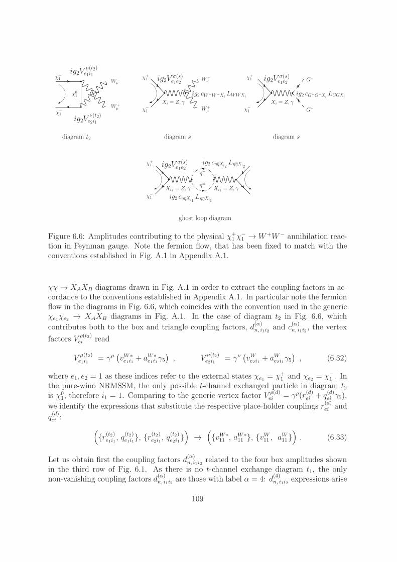
diagram t2
χ01
W+µ
W−ν
χ−1
χ+1
ig2Vµ(t2)e1i1
ig2Vν(t2)e2i1
diagram s
χ+1
χ−1 W+µ
W−ν
Xi = Z, γ
χ+1
χ−1
Xi = Z, γ
G+
G−
diagram s
ig2Vσ(s)e1e2
ig2 cW+W−Xi LWWXi ig2 cG+G−Xi LGGXi
ig2Vσ(s)e1e2
ghost loop diagram
χ+1
χ−1
η±
η±
Xi1 = Z, γ
ig2Vσ(s)e1e2
ig2 cηηXi1 LηηXi1
Xi2 = Z, γ
ig2 cηηXi2 LηηXi2
Figure 6.6: Amplitudes contributing to the physical χ+1 χ
−1 →W+W− annihilation reac-
tion in Feynman gauge. Note the fermion flow, that has been fixed to match with theconventions established in Fig. A.1 in Appendix A.1.
χχ→ XAXB diagrams drawn in Fig. A.1 in order to extract the coupling factors in ac-cordance to the conventions established in Appendix A.1. In particular note the fermionflow in the diagrams in Fig. 6.6, which coincides with the convention used in the genericχe1χe2 → XAXB diagrams in Fig. A.1. In the case of diagram t2 in Fig. 6.6, which
contributes both to the box and triangle coupling factors, d(α)n, i1i2
and c(α)n, i1i2
, the vertex
factors Vρ(t2)ei read
Vµ(t2)e1i1
= γµ(vW∗e1i1
+ aW∗e1i1
γ5), V
ν(t2)e2i1
= γν(vWe2i1 + aWe2i1γ5
), (6.32)
where e1, e2 = 1 as these indices refer to the external states χe1 = χ+1 and χe2 = χ−
1 . Inthe pure-wino NRMSSM, the only possible t-channel exchanged particle in diagram t2is χ0
1, therefore i1 = 1. Comparing to the generic vertex factor Vρ(d)ei = γρ(r
(d)ei + q
(d)ei γ5),
we identify the expressions that substitute the respective place-holder couplings r(d)ei and
q(d)ei :
(r(t2)e1i1
, q(t2)e1i1, r(t2)e2i1
, q(t2)e2i1)→
(vW∗
11 , aW∗11 , vW11 , aW11
). (6.33)
Let us obtain first the coupling factors d(α)n, i1i2
related to the four box amplitudes shownin the third row of Fig. 6.1. As there is no t-channel exchange diagram t1, the onlynon-vanishing coupling factors d
(α)n, i1i2
are those with label α = 4: d(4)n, i1i2
expressions arise
109
from the product of coupling factors in χe1χe2 → XAXB annihilation diagrams of typet2 with the complex conjugate of the coupling factors associated with χe4χe3 → XAXB
annihilation via diagram type t2.11 The constituent coupling factors for the d
(4)n, i1i2
inχ+1 χ
−1 →W+W− → χ+
1 χ−1 scattering are collected in the following table:
α = 4 :(r(t2)e1i1
, q(t2)e1i1, r(t2)e2i1
, q(t2)e2i1, r(t2)∗e3i2
, q(t2)∗e3i2, r(t2)∗e4i2
, q(t2)∗e4i2)
→(vW∗
11 , aW∗11 , vW11 , aW11, vW∗
11 , aW∗11 , vW11 , aW11
). (6.34)
Selecting one element from each of the four subsets and multiplying these selected el-ements with each other gives rise to the d
(4)n, i1i2
. The label n denotes a string of fourcharacters, that indicates which coupling (type r or q) was selected from the ith subsetin (6.34). For instance
d(4)χ+
1 χ−
1 →W+W−→χ+1 χ
−
1
rrrr, 11 = vW∗11 v
W11v
W∗11 v
W11 . (6.35)
Turning to the coupling factors in triangle and selfenergy amplitudes, c(α)n, i1i2
and bn, i1i2 ,they receive contributions from the s-channel diagrams in Fig. 6.6. We proceed in asimilar way as done for the diagram t2 and identify the following coupling factors for thecase of single s-channel Z-exchange (first line) and single s-channel γ-exchange (secondline):
Vσ(s)11 = γσ
(vZ11 + aZ11γ5
), cW+W−Z = cW ,
Vσ(s)11 = γσ (vγ11 + aγ11γ5) , cW+W−γ = sW . (6.36)
The building blocks for the bn, i1i2 , c(α)n, i1i2
and finally these expressions themselves can now
be obtained in a similar manner as described for the d(α)n, i1i2
expressions. However, beforeproceeding with their explicit construction, significant simplifications can be performedby noting that the pure-wino NRMSSM exhibits a particularly simple coupling structure:the (axial-)vector couplings of χ0
1 and χ±1 to the Standard Model gauge bosons are given
by
vW11 = 1 , aW11 = 0 , vγ11 = −sW , aγ11 = 0 ,
vZ11 = −cW , aZ11 = 0 . (6.37)
With the vanishing of all axial-vector couplings the only non-vanishing coupling factord(α)n, i1i2
for χ+1 χ
−1 →W+W− → χ+
1 χ−1 in the pure-wino NRMSSM hence reads
d(4)χ+
1 χ−
1 →W+W−→χ+1 χ
−
1
rrrr,11 = 1 . (6.38)
The absence of a t-channel exchange diagram t1 implies, that only c(α)n, i1i2
factors withα = 3, 4 can be non-vanishing, as these are built from vertex coupling factors associated
11For further conventions on the enumeration label α see Appendix A.1.
110
with diagram type t2 and diagram type s, see Fig. 6.1. In the pure-wino NRMSSM, wefind the following expressions
c(α=3,4)χ+
1 χ−
1 →W+W−→χ+1 χ
−
1
rrr, 1Z = −c2W , c(α=3,4)χ+
1 χ−
1 →W+W−→χ+1 χ
−
1
rrr, 1γ = −s2W , (6.39)
and all other c(α)n, 1i2
vanish. Finally, the non-zero factors bn, i1i2 read
brr, ZZ = c4W , brr, Zγ = brr, γZ = c2W s2W , brr, γγ = s4W , (6.40)
where we have suppressed the superscript χ+1 χ
−1 → W+W− → χ+
1 χ−1 to shorten the
notation. A similar procedure leads to the coupling factors in χ+1 χ
−1 → XAXB rates
with the (unphysical) final states XAXB = G+G−, η+η+ and η−η−. We quote the non-vanishing results for the coupling factors related to χ+
1 χ−1 → G+G− → χ+
1 χ−1 reactions:
brr, ZZ =1
4
(c2W − s2W
)2, brr, Zγ = brr, γZ =
s2W2
(c2W − s2W
),
brr, γγ = s4W . (6.41)
In case of χ+1 χ
−1 → η+η+ → χ+
1 χ−1 and χ+
1 χ−1 → η−η− → χ+
1 χ−1 reactions we find in both
cases the same result (again suppressing the process-specifying superscripts):
brr, ZZ = c4W , brr, Zγ = brr, γZ = c2W s2W , brr, γγ = s4W . (6.42)
6.3.2 Kinematic factors
As for the coupling factors, the kinematic factors Bn, i1i2 , C(α)n, i1X
, D(α)n, i1i2
reduce to verysimple expressions in the pure-wino NRMSSM. Again we rely in this section on conven-tions introduced in the appendices, in particular in Appendices A.2 and A.3. For thenotation used in the following, the reader is therefore referred to these chapters.
As the hard annihilation reactions in the pure-wino NRMSSM refer to the limit ofvanishing SU(2)L gauge boson masses, the relevant (mass) parameters in any of theχe1χe2 → XAXB → χe4χe3 scattering reactions with χea = χ0
1, χ±1 read
m = m = mχ , M = 2 mχ , ∆AB = 0 ,
β = 1 , P sZ,γ = 1 , P1AB =
1
2. (6.43)
Further, the rescaled quantity mi1,2 in the pure-wino limit reads m1 = 1/2 if it refers tothe χ0
1 or χ±1 species and it vanishes if related to Z and γ, mZ,γ = 0. Taking the relations
(6.43) into account, we obtain concise analytic results for the kinematic factors relevantin χ+
1 χ−1 → XAXB → χ+
1 χ−1 scattering. These are collected in Tab. 6.2. Note that we
have given only those kinematic factors that are associated with non-vanishing couplingfactors in the physical χ+
1 χ−1 →W+W− → χ+
1 χ−1 reaction. Assembling and inserting the
above results into the master formula (6.17) we find the results for the absorptive part
111
1S03S1
1P13PJ
1S(p2)0
3S(p2)1
BV Vrr,V V (
2s+1LJ) 0 − 196
0 0 0 1529
C(α=3,4)V Vrrr,1V (2s+1LJ ) 0 − 4
30 0 0 64
9
D(4)V Vrrrr,11(
2s+1LJ) 2 23
83
563
−323
−329
BSSrr,V V (
2s+1LJ) 0 13
0 0 0 −169
Bηηrr,V V (
2s+1LJ) 0 − 112
0 0 0 49
Table 6.2: Kinematic factors for partial-wave reactions up to O(v2rel) in the pure-winoNRMSSM, relevant for the determination of the χ+
1 χ−1 → W+W− annihilation rate. The
subscript label V on the kinematic factors B and C above refers to both the cases of Zand γ single s-channel exchange in the (tree-level) annihilation amplitudes. The resultsfor the kinematic factor B in the last line apply to ηη = η+η+, η−η−.
of the Wilson coefficients that provide the χ+1 χ
−1 → W+W− annihilation cross section
(6.24). For 3S1 annihilation we have
fχ+1 χ
−
1 →W+W−→χ+1 χ
−
1
1111 (3S1)
=πα2
2
4m2χ
(∑
n=rr
∑
i1,i2=Z,γ
bχ+1 χ
−
1 →W+W−→χ+1 χ
−
1
n, i1i2B V Vn, i1i2(
3S1)
+∑
α=3,4
∑
n=rrr
∑
i1=1,i2=Z,γ
c(α)χ+
1 χ−
1 →W+W−→χ+1 χ
−
1
n, i1i2C
(α) V Vn, i1i2
(3S1)
+∑
α=4
∑
n=rrrr
∑
i1,i2=1
d(α)χ+
1 χ−
1 →W+W−→χ+1 χ
−
1
n, i1i2D
(α)V Vn, i1i2
(3S1)
+∑
n=rr
∑
i1,i2=Z,γ
bχ+1 χ
−
1 →G+G−→χ+1 χ
−
1
n, i1i2B SSn, i1i2(
3S1)
+∑
η=η±
∑
n=rr
∑
i1,i2=Z,γ
bχ+1 χ
−
1 →ηη→χ+1 χ
−
1
n, i1i2B ηηn, i1i2
(3S1)
)
=πα2
2
4m2χ
((c4W + c2W s
2W + s4W
)×(−19
6
)+ 2
(−c2W − s2W
)×(−43
)
112
+ 1× 2
3+
1
4× 1
3− 2× 1
12
)
=1
48
πα22
m2χ
, (6.44)
where we have summed over all (unphysical) final states in Feynman gauge, XAXB =W+W−, G+G−, η+η+, η−η−, that contribute to the physical χ+
1 χ−1 →W+W− rate in the
pure-wino NRMSSM scenario. In case of the 1S0 annihilation reaction only the piecesrelated to the α = 4 box amplitude contribute, and the only non-vanishing couplingfactor d
(4)n, i1i2
is d(4)rrrr ,11 given in (6.38), therefore
fχ+1 χ
−
1 →W+W−→χ+1 χ
−
1
1111 (1S0) =πα2
2
4m2χ
d(4)χ+
1 χ−
1 →W+W−→χ+1 χ
−
1
rrrr,11 D(4) V Vrrrr, 11(
1S0)
=πα2
2
2m2χ
. (6.45)
Finally, the absorptive parts of the O(v2rel) partial-wave Wilson coefficients read
fχ+1 χ
−
1 →W+W−→χ+1 χ
−
1
1111 (1P1) =2πα2
2
3m2χ
, fχ+1 χ
−
1 →W+W−→χ+1 χ
−
1
1111 (3PJ ) =14πα2
2
3m2χ
,
gχ+1 χ
−
1 →W+W−→χ+1 χ
−
1
1111 (1S0) = − 8πα22
3m2χ
, gχ+1 χ
−
1 →W+W−→χ+1 χ
−
1
1111 (3S1) = − πα22
9m2χ
. (6.46)
Following (6.24), the non-relativistic expansion of the χ+1 χ
−1 → W+W− annihilation
cross section in the pure-wino NRMSSM is given by
σχ+1 χ
−
1 →W+W−
vrel = a + (bP + bS) v2rel + O(v4rel)
=9
16
πα22
m2χ
+
(1
3− 3
16
)πα2
2
m2χ
v2rel + O(v4rel) ,
=9
16
πα22
m2χ
+7
48
πα22
m2χ
v2rel + O(v4rel) . (6.47)
The values for the parameters a, bP and bS, that one obtains for a pure-wino NRMSSMmass scale mχ = 2748.92GeV read a = 3.06 · 10−27 cm3 s−1, bP c
2 = 1.81 · 10−27 cm3 s−1
and bS c2 = −1.02 · 10−27 cm3 s−1. The mass scale mχ agrees with the neutralino LSP
mass of the MSSM scenario introduced in Sec. 6.2. The latter MSSM scenario features asmall but non-vanishing Higgsino admixture to the wino-like χ0
1 and χ±1 : the Higgsino-
like neutralino and chargino states are not at all decoupled but reside at the scale of∼ 2.9−3TeV. Thus we should not expect the results for the wino-like scenario of Sec. 6.2to be approximated by the pure-wino NRMSSM. This is in fact what the comparison ofthe parameters a, bP and bS for the χ+
1 χ−1 → W+W− annihilation cross section shows:
the corresponding parameters in the MSSM scenario investigated in Sec. 6.2 were given
113
by a = 2.65 · 10−27 cm3 s−1, bP c2 = 1.86 · 10−27 cm3 s−1, bS c
2 = −0.88 · 10−27 cm3 s−1.The results for the S-wave parameters a and bS in the pure-wino χ+
1 χ−1 → W+W−
reaction are a bit larger, which is a consequence of the larger couplings of the pure-wino neutralino and chargino states to the SU(2)L gauge bosons and the absence oft-channel annihilation into the (unphysical) final state G+G−. Due to the non-decoupledhiggsino-like neutralino states in the scenario of Sec. 6.2 the latter contribution is presentand interferes destructively with the corresponding s-channel exchange contribution alsopresent in the pure-wino NRMSSM limit. This leads to a suppression of the a andbS cross section parameters in the wino-like scenario of Sec. 6.2 with respect to thepure-wino NRMSSM. On the contrary the parameter bP turns out to be somewhatlarger in the Sec. 6.2 scenario which traces back to the non-vanishing P -wave t-channelannihilations into G+G− final states that are absent in the pure-wino NRMSSM. Notethat the χ+χ− →W+W− annihilation cross section for the Sec. 6.2 scenario in additionexhibits non-vanishing contributions from the (unphysical) V S = W±G∓ final states notpresent in the pure-wino NRMSSM. These are however suppressed with respect to theXAXB = W+W−, G+G− contributions.
6.3.3 Exclusive pure-wino NRMSSM co-annihilation rates
We conclude the discussion of the short distance (tree-level) annihilation rates in thepure-wino NRMSSM by collecting results for all exclusive (physical) XAXB final statecontributions to the Wilson coefficients f , g that determine the (off-) diagonal co-an-nihilation rates χe1χe2 → XAXB → χe4χe3 in this scenario. The non-relativistic expan-sion of the respective exclusive rates can then be obtained from (6.22) and (6.30). Forconvenience we write the pure-wino NRMSSM Wilson coefficients as
f χe1χe2
→XAXB→χe4χe3
(2s+1LJ
)=
πα22
m2χ
cχe1χe2
→XAXB→χe4χe3
(2s+1LJ
). (6.48)
In case of the next-to-next-to-leading order S-wave coefficients we establish a similarnotation with f replaced by g on the l.h.s. of (6.48) and the 2s+1LJ = 1S0,
3S1 label of
the factor c on the r.h.s. substituted by 1S(p2)0 , 3S
(p2)1 . Note that the Wilson coefficients
hi always vanish in the hard annihilation rates in the pure-wino NRMSSM due to thecomplete mass-degeneracy of the χ0
1 and χ±1 states.
At the beginning of Sec. 6.3 we have already noted, that the calculation of thehard annihilation rates in the pure-wino NRMSSM toy-scenario refers to massless SMgauge bosons and SM fermions. These can hence appear as possible XAXB final stateparticles in the χe1χe2 → XAXB → χe4χe3 reactions. As far as the Higgs-sector isconcerned we present in this section results that refer to the decoupling limit [95] inthe underlying MSSM scenario: we assume a SM-like CP -even Higgs boson h0 in thelow-energy spectrum of the theory while the heavier Higgs states A0, H0, H± are entirelydecoupled (mA0 ∼ mH0 ∼ mH+ ≫ mχ ≫ 0). As generically mh0 < mZ at tree-levelin the MSSM, the h0 is consequently treated as massless in the pure-wino NRMSSMhard annihilation rates. According to their overall charge the (co-)annihilation processes
114
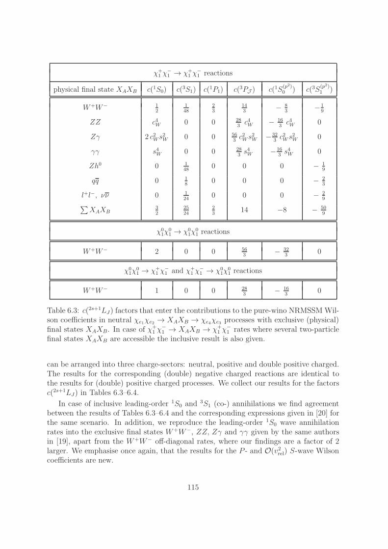
χ+1 χ
−1 → χ+
1 χ−1 reactions
physical final state XAXB c(1S0) c(3S1) c(1P1) c(3PJ ) c(1S(p2)0 ) c(3S
(p2)1 )
W+W− 12
148
23
143
− 83
−19
ZZ c4W 0 0 283c4W − 16
3c4W 0
Zγ 2 c2Ws2W 0 0 56
3c2W s
2W −32
3c2Ws
2W 0
γγ s4W 0 0 283s4W −16
3s4W 0
Zh0 0 148
0 0 0 − 19
qq 0 18
0 0 0 − 23
l+l−, νν 0 124
0 0 0 − 29
∑XAXB
32
2524
23
14 −8 − 509
χ01χ
01 → χ0
1χ01 reactions
W+W− 2 0 0 563
− 323
0
χ01χ
01 → χ+
1 χ−1 and χ+
1 χ−1 → χ0
1χ01 reactions
W+W− 1 0 0 283
− 163
0
Table 6.3: c(2s+1LJ) factors that enter the contributions to the pure-wino NRMSSMWil-son coefficients in neutral χe1χe2 → XAXB → χe4χe3 processes with exclusive (physical)final states XAXB. In case of χ+
1 χ−1 → XAXB → χ+
1 χ−1 rates where several two-particle
final states XAXB are accessible the inclusive result is also given.
can be arranged into three charge-sectors: neutral, positive and double positive charged.The results for the corresponding (double) negative charged reactions are identical tothe results for (double) positive charged processes. We collect our results for the factorsc(2s+1LJ) in Tables 6.3–6.4.
In case of inclusive leading-order 1S0 and 3S1 (co-) annihilations we find agreementbetween the results of Tables 6.3–6.4 and the corresponding expressions given in [20] forthe same scenario. In addition, we reproduce the leading-order 1S0 wave annihilationrates into the exclusive final states W+W−, ZZ, Zγ and γγ given by the same authorsin [19], apart from the W+W− off-diagonal rates, where our findings are a factor of 2larger. We emphasise once again, that the results for the P - and O(v2rel) S-wave Wilsoncoefficients are new.
115
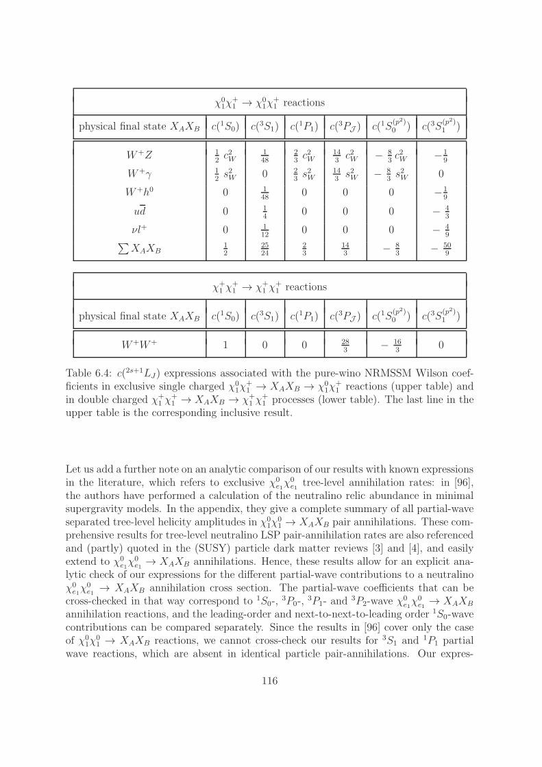
χ01χ
+1 → χ0
1χ+1 reactions
physical final state XAXB c(1S0) c(3S1) c(1P1) c(3PJ ) c(1S(p2)0 ) c(3S
(p2)1 )
W+Z 12c2W
148
23c2W
143c2W − 8
3c2W −1
9
W+γ 12s2W 0 2
3s2W
143s2W − 8
3s2W 0
W+h0 0 148
0 0 0 −19
ud 0 14
0 0 0 − 43
νl+ 0 112
0 0 0 − 49∑
XAXB12
2524
23
143
− 83
− 509
χ+1 χ
+1 → χ+
1 χ+1 reactions
physical final state XAXB c(1S0) c(3S1) c(1P1) c(3PJ ) c(1S(p2)0 ) c(3S
(p2)1 )
W+W+ 1 0 0 283
− 163
0
Table 6.4: c(2s+1LJ) expressions associated with the pure-wino NRMSSM Wilson coef-ficients in exclusive single charged χ0
1χ+1 → XAXB → χ0
1χ+1 reactions (upper table) and
in double charged χ+1 χ
+1 → XAXB → χ+
1 χ+1 processes (lower table). The last line in the
upper table is the corresponding inclusive result.
Let us add a further note on an analytic comparison of our results with known expressionsin the literature, which refers to exclusive χ0
e1χ0e1 tree-level annihilation rates: in [96],
the authors have performed a calculation of the neutralino relic abundance in minimalsupergravity models. In the appendix, they give a complete summary of all partial-waveseparated tree-level helicity amplitudes in χ0
1χ01 → XAXB pair annihilations. These com-
prehensive results for tree-level neutralino LSP pair-annihilation rates are also referencedand (partly) quoted in the (SUSY) particle dark matter reviews [3] and [4], and easilyextend to χ0
e1χ0e1→ XAXB annihilations. Hence, these results allow for an explicit ana-
lytic check of our expressions for the different partial-wave contributions to a neutralinoχ0e1χ
0e1 → XAXB annihilation cross section. The partial-wave coefficients that can be
cross-checked in that way correspond to 1S0-,3P0-,
3P1- and3P2-wave χ
0e1χ0e1→ XAXB
annihilation reactions, and the leading-order and next-to-next-to-leading order 1S0-wavecontributions can be compared separately. Since the results in [96] cover only the caseof χ0
1χ01 → XAXB reactions, we cannot cross-check our results for 3S1 and 1P1 partial
wave reactions, which are absent in identical particle pair-annihilations. Our expres-
116
sions for the partial-wave separated χ0e1χ0e1→ XAXB annihilation cross sections into all
possible SM and Higgs final states, obtained from (6.22), agree with the correspondingterms derived from the helicity amplitudes in [96]12. Let us finally note that our resultsfor annihilations into a pair of fermions include the case of flavour-off-diagonal sfermionmixing as well, which is covered in [3] and [4], but was not yet included in [96], whereinonly flavour-diagonal right-left sfermion mixing was taken into account, although it isstraightforward to extend these results to the general flavour-off-diagonal case.
12The only minor discrepancies that we find are related to P -wave contributions: our results for 3P1-wave χ0
e1χ0e1 → H+H− annihilations correspond to a factor 2 instead of a factor 4 in the second term
of Eq. (A27b) in [96]. In the case of 3P0-wave χ0e1χ
0e1 → f f reactions, our results correspond to a factor√
2/3 instead of a factor√6 in the second term in the first line of Eq. (A29b) in [96].
117

118
Chapter 7
Long-range potential interactions
The instantaneous but spatially non-local long-range potential interactions that even-tually cause the Sommerfeld enhancement of χχ pair-annihilation cross sections in thenon-relativistic regime are encoded in the part Lpot of the effective field theory La-grangian LNRMSSM introduced in Sec. 5.1. In (5.3) we have already given the genericform of the contributions to Lpot. Here we explicitly determine the coefficients of thefour-fermion operators in Lpot at leading order in the non-relativistic expansion, whichare given by Yukawa- and Coulomb-potentials associated with electroweak gauge or Higgsboson mediator particles. The corresponding matching calculation that provides explicitanalytical expressions for the potentials in terms of MSSM parameters and couplingsis the content of Sec. 7.1, where we use the example of potential Z-boson exchangeto illustrate the procedure. Explicit expressions that allow to build all leading-orderNRMSSM potentials are collected in Appendix B. In Sec. 7.2 we subsequently discussthe representation of potential interactions as well as hard annihilation reactions in theNRMSSM in terms of corresponding potential and annihilation matrices. This requiresthe definition of a suitable basis of NRMSSM two-particles states (χχ)I=1,...,N . The twopossible choices, one basis which contains and counts as different the states χe1χe2 andχe2χe1 with non-identical particles χea and χeb, the other where the redundant statesχe2χe1 are absent, are discussed in Sec. 7.2.1. To complete the presentation of resultsrelated to the pure-wino NRMSSM in Sec. 6.3 we finally provide in Sec. 7.2.2 explicitanalytic expressions for the potential and annihilation matrices in that scenario, usingboth the basis with and without redundant χχ states.
7.1 NRMSSM potentials: Matching calculation
In Sec. 2.1 we have discussed ladder diagrams in non-relativistic χχ → χχ scatteringwith light mediator exchange in order to understand the origin of the Sommerfeld en-hancement effect starting from amplitudes in the full theory. The enhancement effectcould be attributed to particularly large contributions to the individual loop integralsin the ladder diagram that arise in the region where the loop momenta have potential
119
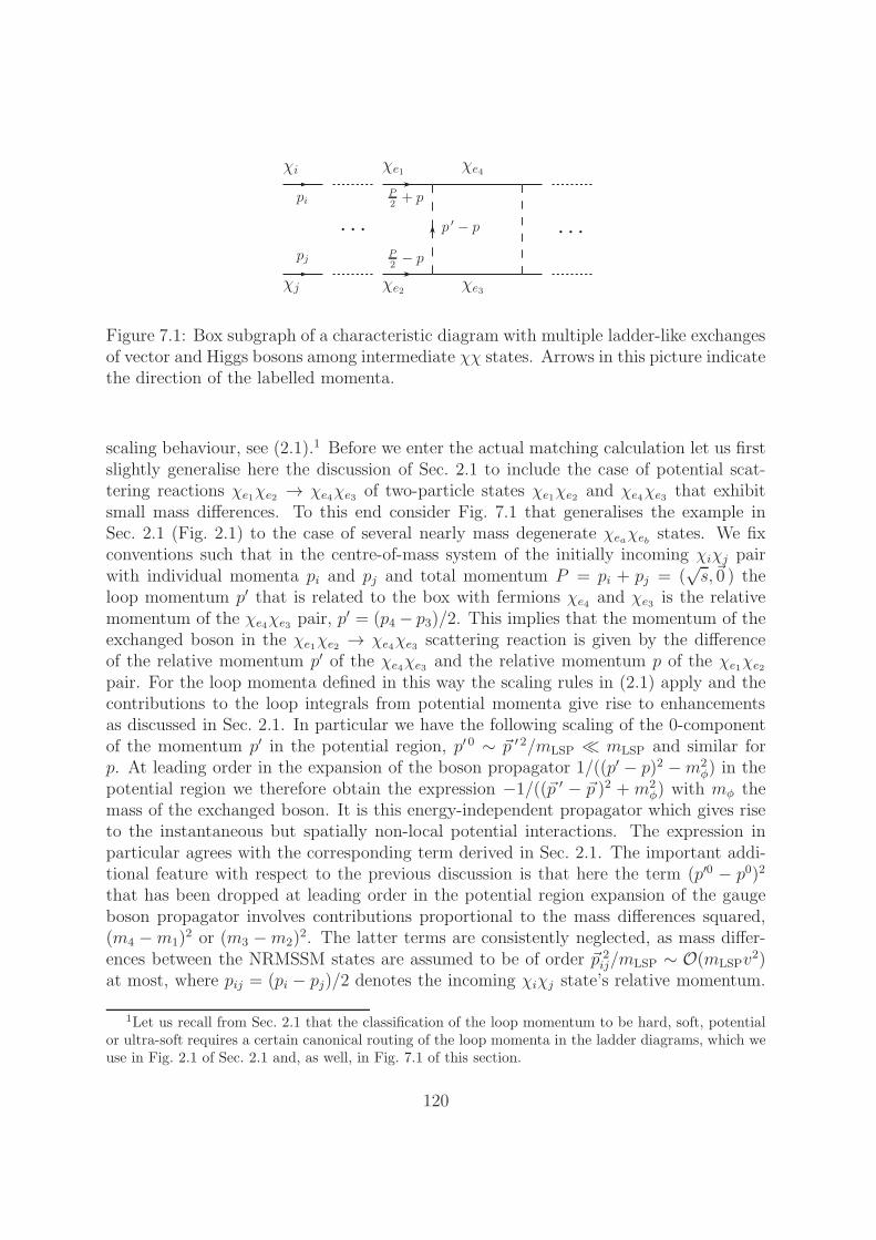
χe1
p ′ − p
χe4
χe2 χe3χj
χiP2+ p
P2− p
pi
pj
Figure 7.1: Box subgraph of a characteristic diagram with multiple ladder-like exchangesof vector and Higgs bosons among intermediate χχ states. Arrows in this picture indicatethe direction of the labelled momenta.
scaling behaviour, see (2.1).1 Before we enter the actual matching calculation let us firstslightly generalise here the discussion of Sec. 2.1 to include the case of potential scat-tering reactions χe1χe2 → χe4χe3 of two-particle states χe1χe2 and χe4χe3 that exhibitsmall mass differences. To this end consider Fig. 7.1 that generalises the example inSec. 2.1 (Fig. 2.1) to the case of several nearly mass degenerate χeaχeb states. We fixconventions such that in the centre-of-mass system of the initially incoming χiχj pairwith individual momenta pi and pj and total momentum P = pi + pj = (
√s,~0 ) the
loop momentum p′ that is related to the box with fermions χe4 and χe3 is the relativemomentum of the χe4χe3 pair, p′ = (p4 − p3)/2. This implies that the momentum of theexchanged boson in the χe1χe2 → χe4χe3 scattering reaction is given by the differenceof the relative momentum p′ of the χe4χe3 and the relative momentum p of the χe1χe2pair. For the loop momenta defined in this way the scaling rules in (2.1) apply and thecontributions to the loop integrals from potential momenta give rise to enhancementsas discussed in Sec. 2.1. In particular we have the following scaling of the 0-componentof the momentum p′ in the potential region, p′ 0 ∼ ~p ′ 2/mLSP ≪ mLSP and similar forp. At leading order in the expansion of the boson propagator 1/((p′ − p)2 −m2
φ) in thepotential region we therefore obtain the expression −1/((~p ′ − ~p )2 + m2
φ) with mφ themass of the exchanged boson. It is this energy-independent propagator which gives riseto the instantaneous but spatially non-local potential interactions. The expression inparticular agrees with the corresponding term derived in Sec. 2.1. The important addi-tional feature with respect to the previous discussion is that here the term (p′0 − p0)2that has been dropped at leading order in the potential region expansion of the gaugeboson propagator involves contributions proportional to the mass differences squared,(m4 −m1)
2 or (m3 −m2)2. The latter terms are consistently neglected, as mass differ-
ences between the NRMSSM states are assumed to be of order ~p 2ij/mLSP ∼ O(mLSPv
2)at most, where pij = (pi − pj)/2 denotes the incoming χiχj state’s relative momentum.
1Let us recall from Sec. 2.1 that the classification of the loop momentum to be hard, soft, potentialor ultra-soft requires a certain canonical routing of the loop momenta in the ladder diagrams, which weuse in Fig. 2.1 of Sec. 2.1 and, as well, in Fig. 7.1 of this section.
120
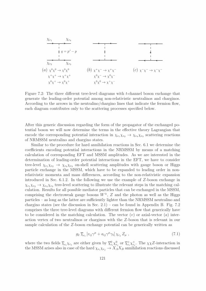
χe1
q = p ′ − p
χe4
χe2 χe3
χ0χ0 → χ0χ0
χ+χ+ → χ+χ+
χ0χ+ → χ0χ+
χ+χ− → χ+χ−
χ0χ− → χ0χ−
(a) (b) (c) χ−χ− → χ−χ−
χ0χ0 → χ+χ−
Figure 7.2: The three different tree-level diagrams with t-channel boson exchange thatgenerate the leading-order potential among non-relativistic neutralinos and charginos.According to the arrows in the neutralino/chargino lines that indicate the fermion flow,each diagram contributes only to the scattering processes specified below.
After this generic discussion regarding the form of the propagator of the exchanged po-tential boson we will now determine the terms in the effective theory Lagrangian thatencode the corresponding potential interaction in χe1χe2 → χe4χe3 scattering reactionsof NRMSSM neutralino and chargino states.
Similar to the procedure for hard annihilation reactions in Sec. 6.1 we determine thecoefficients encoding potential interactions in the NRMSSM by means of a matchingcalculation of corresponding EFT and MSSM amplitudes. As we are interested in thedetermination of leading-order potential interactions in the EFT, we have to considertree-level χe1χe2 → χe4χe3 on-shell scattering amplitudes with gauge boson or Higgsparticle exchange in the MSSM, which have to be expanded to leading order in non-relativistic momenta and mass differences, according to the non-relativistic expansionintroduced in Sec. 6.1.2. In the following we use the example of Z-boson exchange inχe1χe2 → χe4χe3 tree-level scattering to illustrate the relevant steps in the matching cal-culation. Results for all possible mediator particles that can be exchanged in the MSSM,comprising the electroweak gauge bosons W±, Z and the photon as well as the Higgsparticles – as long as the latter are sufficiently lighter than the NRMSSM neutralino andchargino states (see the discussion in Sec. 2.1) – can be found in Appendix B. Fig. 7.2comprises the three tree-level diagrams with different fermion flow that generically haveto be considered in the matching calculation. The vector (v) or axial-vector (a) inter-action vertex of two neutralinos or charginos with the Z-boson that is relevant in oursample calculation of the Z-boson exchange potential can be generically written as
g2 χei [vijγµ + aijγ
µγ5]χej Zµ , (7.1)
where the two fields χeiχej are either given by χ0eiχ0ej
or χ+eiχ+ej. The χχZ-interaction in
the MSSM arises also in case of the hard χeiχej → XAXB annihilation reactions discussed
121
in Chap. 6 and explicit expressions for the vertex factors vij and aij are provided inAppendix A.1.2.2
As regards the determination of the leading-order Z-exchange potential we start fromthe on-shell scattering amplitude in Fig. 7.2(a) and expand the full-theory amplitude inthe small relative momenta ~p, ~p ′ ∼ mLSPvrel ∼ MZ as well as in p0, p′ 0 ∼ mLSPv
2rel,
keeping only the leading-order terms. This implies an expansion of the Dirac bilinearsu(p4)Γu(p1)u(p3)Γu(p2) associated with the amplitude, where Γ and Γ stand for a certaincombination of the structures 14×4, γµ, γ5, q/ with q = p4 − p1 = p2 − p3, as well as acorresponding expansion of the Z-boson propagator
−iq2 −M2
Z
(gµν −
qµqνM2
Z
)+
qµqνM2
Z
−iq2 − ξM2
Z
, (7.2)
here defined in Rξ-gauge. At leading order the non-relativistic expansion of the formerproduct of Dirac bilinears is equivalent to the following replacements in the full-theoryamplitude:
γµ ⊗ γµ → 1⊗ 1 , γµγ5 ⊗ γµγ5 → −σi ⊗ σi ,γµγ5 ⊗ γµ , γµ ⊗ γµγ5 → 0 ,
q/⊗ q/→ −(me4 −me1)(me3 −me2) 1⊗ 1 ,
q/⊗ q/γ5 , q/γ5 ⊗ q/ , q/γ5 ⊗ q/γ5 → 0 . (7.3)
While the expressions on the left-hand side in these replacement rules are understood toact on the four-component spinors associated with the on-shell fields at the upper andlower interaction vertex in Fig. 7.2(a), the right-hand side terms should be understood asmatrices acting on the two-component Pauli spinors of the corresponding non-relativisticneutralino or chargino fields. Accordingly, the latter spin operators written in componentnotation read σi⊗σi ≡ σiα4α1
σiα3α2and 1⊗1 ≡ δα4α1
δα3α2. Note that as already remarked
in Sec. 6.1, the matching procedure implies the use of the non-relativistic normalisationu(pea)u(pea) = 1 of the four-component spinors. Finally let us point out that the relationin the third line in (7.3) is obtained using the equation of motion for the spinors. Thenon-relativistic scaling of the corresponding term is discussed below. Using (7.3) theleading-order term in the non-relativistic expansion of amplitude Fig. 7.2(a) with Z-boson exchange is given by
(Fig.3a)Z =−ig22
~q 2 +M2Z
[(1 +
δme4e1 δme3e2
M2Z
)vZe4e1v
Ze3e2
1⊗ 1− aZe4e1aZe3e2
σi ⊗ σi]
+ig22
~q 2 + ξM2Z
δme4e1 δme3e2
M2Z
vZe4e1vZe3e2
1⊗ 1 . (7.4)
2Similarly, the vertex factors related to χχW+ and χχγ interactions as well as the scalar (s) andpseudo-scalar (p) vertex factors associated with χχ-Higgs three-point interactions can be found in thisappendix. All such interactions can arise in potential χe1χe2 → χe4χe3 tree-level scattering reactionsand the corresponding vertex factors enter the explicit expressions for the respective potentials fromgauge boson (Z,W±, γ) or Higgs particle (h0, H0, A0, H±) exchange collected in Appendix B.
122

For simplicity this expression refers to the case of χ0χ0 → χ0χ0 or χ+χ+ → χ+χ+
scattering reactions where the type of (axial-)vector couplings at both the upper andlower vertices in Fig. 7.2(a) is the same, namely either related to χ0χ0Z or to χ+χ−Zthree-point interactions. The extension to χ0χ+ → χ0χ+ processes where the vector andaxial-vector couplings related to both the χ0χ0Z and χ+χ−Z vertex arise is straightfor-ward.
Before we comment on the expression in the first line in (7.4) that involves theproduct of mass differences, δme4e1δme3e2 , let us first discuss the term in the secondline. This term arises from the ξ-dependent term in the Z-boson propagator in (7.2).Due to gauge invariance it has to cancel against the contribution from Goldstone bosonA0
2 ≡ G0 exchange, where the Goldstone boson mass is given by mG0 = ξM2Z . Such
cancellation takes place as certain relations among the vector and scalar couplings ofthe neutralinos and charginos hold within the MSSM: the leading-order contribution inthe non-relativistic expansion of the amplitude Fig. 7.2(a) with scalar boson φ exchangereads
(Fig.3a)φ =ig22
~q 2 +m2φ
sφe4e1sφe3e2
1⊗ 1 . (7.5)
Pseudo-scalar interactions do not survive in (7.5) because at leading order in the non-relativistic expansion the replacements 1 ⊗ γ5, γ5 ⊗ 1, γ5 ⊗ γ5 → 0, relevant in the caseof amplitudes with scalar particle exchange, complement among others the replacementrules in (7.3). For a cancellation of the ξ-dependent terms in (7.4) and (7.5) the condition
δme4e1 δme3e2
M2Z
vZe4e1vZe3e2 + sG
0
e4e1sG0
e3e2 = 0 (7.6)
must hold, implying that the relations vZij (mi − mj)/MZ = ±isG0
ij must be fulfilled.The latter relations can be proven using the explicit expressions of the couplings vZ
and sG0
in terms of mixing matrices and couplings given in Appendix A.1.2, as wellas the diagonalisation properties of the mixing matrices. Consequently we can dropthe ξ-dependent contributions in (7.4) together with the Goldstone boson G0-exchangecontributions (7.5). Similar cancellation take, for instance, place in case of potentialχe1χe2 → χe4χe3 scattering with W+- and G+-exchange, such that we can eventuallyconsider only ξ-independent contributions to the potential interactions that are relatedto the exchange of physical states, leaving out the case of potential Goldstone bosons inthe diagrams of Fig. 7.2.
As regards the δme4e1δme3e2 proportional term in the first line of (7.4) – which is re-lated to expressions involving q/⊗q/ in the unexpanded full-theory amplitude – it typicallyyields a very small contribution, since the effective theory contains only those speciesthat give rise to mass differences δm ∼ O(mLSPv
2rel). Even for a spectrum with heavy χ0
1
where mLSPv2rel ≫MZ is possible for non-relativistic NRMSSM states, the δme4e1δme3e2
proportional term gives O(1) contributions at most due to suppressed vector couplings.This can be seen in the decoupling limit mLSP → ∞. As long as the mass differ-ence δmeaeb refers to particles χea , χeb within the same electroweak multiplet it scales
123
as δmeaeb ∼ M2EW/mLSP, such that the mass difference terms in (7.4) are suppressed as
δmeaeb/MZ ∼ MEW/mLSP. If to the contrary the particles χea , χeb belong to differentmultiplets, the terms δmeaeb/MZ can be large but are multiplied by suppressed couplingsvZeaeb ∼ MEW/δmeaeb following (7.6). Finally let us note that the axial-vector couplingsgo to zero in the decoupling limit such that the gauge-independent, off-diagonal termsin square brackets in the first line in (7.4) are in this case given by the pseudo Goldstoneboson couplings −sG0
e4e1sG0
e3e2.Instead of performing the same non-relativistic expansion again in order to obtain the
leading-order terms for amplitudes (b) and (c) with Z-boson or neutral scalar φ exchangein Fig. 7.2 we can derive them directly from the corresponding expressions for amplitude(a) in (7.4) and (7.5). Only certain labels on the vertex factors as well as signs in frontof these factors have to be interchanged, where the corresponding replacement rules canbe obtained by a simple adaption of the rules 1. and 2. given in Appendix A.1.2: Ifthe fermion flow on a line of diagram (b) or (c) is reversed with respect to amplitude(a) we need to interchange the labels on the corresponding vertex factors (for instance,Xe3e2 → Xe2e3 to go from (a) to (b)) and change the sign of the corresponding vectorcoupling. In this way we obtain
(Fig.3b)Z =ig22
~q 2 +M2Z
[ (1 +
δme4e1 δme3e2
M2Z
)vZe4e1v
Ze2e3 1⊗ 1+ aZe4e1a
Ze2e3 σ
i ⊗ σi]
− ig22~q 2 + ξM2
Z
δme4e1 δme3e2
M2Z
vZe4e1vZe2e3
1⊗ 1 ,
(Fig.3b)φ =ig22
~q 2 +m2φ
sφe4e1sφe2e3
1⊗ 1 , (7.7)
as well as
(Fig.3c)Z =−ig22
~q 2 +M2Z
[(1 +
δme4e1 δme3e2
M2Z
)vZe1e4v
Ze2e3
1⊗ 1− aZe1e4aZe2e3
σi ⊗ σi]
+ig22
~q 2 + ξM2Z
δme4e1 δme3e2
M2Z
vZe1e4vZe2e3
1⊗ 1 ,
(Fig.3c)φ =ig22
~q 2 +m2φ
sφe1e4sφe2e3 1⊗ 1 . (7.8)
Similar expressions for the leading-order contributions to potential χe1χe2 → χe4χe3scattering processes generated by photon exchange can be obtained from the above Z-boson exchange case by replacing the corresponding vector couplings (vZ → vγ), settingthe axial-vector couplings as well as the force carrier mass to zero and keeping only the gµνdependent part of the propagator in (7.2). The expressions related to pseudo-Goldstoneboson G0 exchange in (7.5, 7.7) and (7.8) can generically be applied to neutral Higgsboson (h0, H0, A0) exchange by appropriate replacements of the coupling factors and theboson mass. The case of W±-boson and charged scalar boson (H±, G±) exchange arises
124
in χ0χ0 → χ±χ∓, χ±χ∓ → χ0χ0 and χ0χ± → χ±χ0 processes. Note that when applyingthe results in (7.4, 7.5, 7.7, 7.8) to these cases we have – apart from the replacementsof masses – to hermitian conjugate the coupling matrices at vertices involving either aninitial χ+ or a final χ0. This prescription follows from the fact that we provide the vertexfactors for incoming χ0
j and outgoing χ+i in the χ0χ±W± and χ0χ±H±
m vertex factors inAppendix A.1.2; our notation therein is such that the first index in the correspondingvector (scalar) and axial-vector (pseudo-scalar) coupling is related to the outgoing χ+
i ,while the second index refers to the incoming χ0
j , see Fig. A.3.The results provided so far in (7.4, 7.5) as well as in (7.7) and (7.8) refer to the leading-
order potentials in momentum-space. The Schrodinger equation that takes into accountthe resummation of potential gauge and Higgs boson exchange in the ladder diagramssuch as Fig. 7.1 (or Fig. 2.1(a) of Sec. 2.1) will however be written in coordinate-space,see Chap. 2 and Chap 8. The corresponding coordinate-space potentials are obtainedfrom the momentum-space expressions above by Fourier transformation
V χχ→χχe1e2e4e3(r) =
∫d3~q
(2π)3ei~q·~x i T χχ→χχ
e1e2e4e3(~q2) , (7.9)
where T χχ→χχe1e2e4e3
denotes the momentum-space amplitude as given in equations (7.4, 7.5,7.7, 7.8) and r ≡ |~x|. From the identity
∫d3~q
(2π)3ei~q·~x
1
~q 2 +m2=
e−mr
4πr, (7.10)
we obtain the well-known Yukawa-type potentials for amplitudes that involve the ex-change of a massive mediator with mass m. In case of a massless force carrier, m = 0,(7.10) gives the Coulomb potential.3
Before presenting the final form of the leading-order coordinate-space potentials inthe NRMSSM we rewrite the spin operator σi ⊗ σi that appears in the potentials withgauge boson exchange as
σi ⊗ σi = 2(~S 2 − ~s 21 − ~s 2
2 ) = 2~S 2 − 3 (1⊗ 1) , (7.11)
where ~s1 (~s2) denotes the spin operator acting on the particles χe4 and χe1 (χe3 andχe2) at the upper (lower) vertices in the diagrams in Fig. 7.2. In the second equalitywe have replaced ~s 2
1,2 by s(s + 1) (1⊗ 1) = 3/4 (1⊗ 1) for the neutralino and chargino
species. ~S denotes the total spin operator acting on the total spin of the incoming andoutgoing neutralino and chargino pairs χeaχeb ,
~S = ~s1+~s2 ≡ 1/2 (~σ⊗1+1⊗~σ). In the
basis of eigenstates of total spin of the χeaχeb pairs we can replace ~S 2 by its eigenvalueS(S + 1) (1 ⊗ 1) = 2S (1 ⊗ 1) for S = 0, 1, where in particular 1 ⊗ 1 is the identityoperator. Eventually, referring to the basis of total spin we can write the leading-ordercoordinate-space potentials in the NRMSSM in the generic form
V χχ→χχe1e2e4e3(r) = (ae1e2e4e3 − (3− 4S) be1e2e4e3)
e−mXr
r, (7.12)
3Let us note that the +iǫ prescription in the gauge boson propagators of the full theory provides thenecessary regularisation for the m = 0 case in (7.10).
125

for exchange of a gauge boson X with mass mX among the incoming and outgoing pairsχe1χe2 and χe4χe3 . The coefficient be1e2e4e3 is solely built from a product of two axial-vector couplings as can be seen from the terms involving σi⊗σi in the momentum-spacepotentials in (7.4, 7.7, 7.8), together with the relation (7.11). Consequently, be1e2e4e3vanishes for the case of leading-order potentials from scalar boson and photon exchange.A spin-dependence of a generic leading-order potential (7.12) thus arises only in presenceof corresponding non-vanishing axial-vector couplings. We collect explicit expressions forall leading-order NRMSSM potentials from electroweak gauge boson, photon and lightHiggs exchange in Appendix B.
7.2 Matrix representation of NRMSSM potentials
Both the labels on the potentials V χχ→χχe1e2e4e3(r) that arise as coefficients of the four-
fermion operators in Lpot as well as the labels on the Wilson coefficients fχχ→χχe1e2e4e3 of
the four-fermion operators in δLann refer to two-particle states χe1χe2 and χe4χe3. Byanalysis of the perturbative expansion of the χiχj → XAXB annihilation amplitudewith ladder-like gauge and Higgs boson exchanges in the non-relativistic limit, we willshow later in Sec. 8.2 that the amplitude can be written as a product of potentials (7.12)times non-relativistic two-particle propagators related to the corresponding intermediateχeaχeb pairs, integrated over corresponding loop momenta and finally multiplied by an
appropriate short-distance Wilson coefficient f encoding the actual hard annihilation.All parts in this amplitude expression refer to χeaχeb two-particle states rather than theindividual χea and χeb particles. The annihilation reactions including the Sommerfeldenhancement – arising due to the presence of long-range potential interactions whichrequire a consistent resummation of all amplitudes with potential ladder exchanges –are therefore conveniently described using a basis of two-particle states. Consideringsuch a two-particle state basis it is convenient to speak of potential matrices as well asannihilation matrices instead of their components, the potential interactions (7.12) andthe absorptive parts of the Wilson coefficients f discussed in Chap. 6: the entries of thematrices are related to a corresponding specific potential or Wilson coefficient f referringto the 2→ 2 scattering reaction of two-particle basis states χe1χe2 → χe4χe3 .
In context of the heuristic discussion of Sommerfeld enhancements and the corre-sponding Schrodinger equation for certain toy scenarios in Chap. 2 we started alreadyfrom a two-particle state basis. In the NRMSSM we now have to construct the two-particle state basis from the individual neutralino and chargino species in the effectivetheory. There are two options, one where states χeaχeb and χebχea built from non-identical particles are considered as different, the other where the redundant secondstate is not considered. Depending on the convention chosen there are certain combi-natorial factors that have to be taken into account when building from the potentialsV χχ→χχe1e2e4e3(r) and absorptive parts of Wilson coefficients fχχ→χχ
e1e2e4e3 the correspond-ing potential and annihilation matrices. We discuss the two bases and the implicationsfor the potential and annihilation matrices in Sec. 7.2.1. Subsequently we provide as an
126
example in Sec. 7.2.2 the potential and annihilation matrices in the pure-wino NRMSSM.
7.2.1 The two possibles bases of χχ states in the NRMSSM
In the discussion of NRMSSM two-particle states we generically have to take five different(electric) charge sectors into account, as two-particle states built from neutralino andchargino species can have electric charge Q = 0,±1,±2. In each charge sector Q weencounter a certain total number N|Q| of different two-particle states,4 which dependson the choice of the two-particle state basis. In the following we discuss two differentchoices for such basis, termed “method-1” and “method-2” basis, in turn.
In case of n0 neutralino and n+ chargino states in the NRMSSM we encounter n20
neutralino pairs, χ0χ0, and 2n2+ neutral χ±χ∓ states, where we counted as different the
states χeaχeb and χebχea for non-identical species χea , χeb, that arise from interchangingthe particles at the first and second position in the χχ state. Consequently we obtainN0 = n2
0+2n2+ neutral two-particle states. Similarly, the charge Q = ±1 sectors comprise
N1 = 2n0n+ two-particle states and in case of Q = ±2 we have N2 = n2+. If for a given
MSSM spectrum the masses of the four neutralino and the two chargino species are, forinstance, so close to each other that all these species have to be taken into account in theNRMSSM, we confront n0 = 4 and n+ = 2. This implies that potential scattering andannihilation reactions between N0 = 24 neutral two-particle states have to be consideredin the Q = 0 sector. Correspondingly, the single and double charged sectors involveN1 = 16 and N2 = 4 interacting χχ states. Written explicitly we have to consider in this“n0 = 4 and n+ = 2” example the N0 = 24 neutral states
χ01χ
01, χ
01χ
02, χ
01χ
03, χ
01χ
04, χ
02χ
01, χ
02χ
02, χ
02χ
03, χ
02χ
04, χ
03χ
01, . . . , χ
04χ
04,
χ+1 χ
−1 , χ
+1 χ
−2 , χ
+2 χ
−1 , χ
+2 χ
−2 , χ
−1 χ
+1 , χ
−1 χ
+2 , χ
−2 χ
+1 , χ
−2 χ
+2 , (7.13)
as well as the following N1 = 16 states in the two charge Q = ±1 sectors,
χ01χ
±1 , χ
01χ
±2 , χ
02χ
±1 , χ
02χ
±2 , χ
03χ
±1 , χ
03χ
±2 , χ
04χ
±1 , χ
04χ
±2 ,
χ±1 χ
01, χ
±2 χ
01, χ
±1 χ
02, . . . , χ
±2 χ
04 , (7.14)
and finally the N2 = 4 states in the Q = ±2 charge sectors,
χ±1 χ
±1 , χ
±1 χ
±2 , χ
±2 χ
±1 , χ
±2 χ
±2 . (7.15)
The entirety of all N0 + 2N1 + 2N2 = 64 states in (7.13 – 7.15) defines the “method-1basis” of two-particles states in our “n0 = 4 and n+ = 2” example. The adaption tothe case of n0 ≤ 4 and n+ ≤ 2 neutralino and chargino species in the NRMSSM isstraightforward. Note that the order of states in each charge sector in (7.13 – 7.15) isof course a matter of convention. By using the method-1 basis of two-particle states
4Note that our notation implies |Q| = 0, 1, 2; the total number of states in the single-positive andsingle-negative, Q = ±1, (double-positive and double-negative, Q = ±2) charge sector obviously agreesand is denoted by N1 (N2).
127
in the NRMSSM – that is by treating χeaχeb and χebχea for non-identical particles χeaand χeb as different – we can in the construction of potential and annihilation matricesdirectly use the expressions for potentials and Wilson coefficients as derived in Sec. 7.1and Chap. 6: In the calculation of χiχj → XAXB annihilation amplitudes with ladder-like exchanges there are no additional combinatorial factors to be taken into account infront of potentials V or Wilson coefficients f as long as we consider and sum over allmethod-1 basis states that are part of the same charge sector as the annihilating χiχjpair.
The “method-2 basis” that we discuss next has the advantage that it contains lesstwo-particle states than the corresponding method-1 basis. In return the potentials andannihilation matrices to be used in the calculation of χiχj → XAXB annihilation rates inthe method-2 basis have to be calculated from the method 1 expressions (directly relatedto the potentials taken from Sec. 7.1 and Wilson coefficients from Chap. 6) by accountingfor certain combinatorial factors and combinations of different method-1 matrix entries.The method-2 basis is built from all χχ states that differ pairwise with respect to theindividual particle content. This implies that only one of the states χeaχeb and χebχeafor different particle species χea,b is considered as a basis state, the other is redundantand ignored. While this prescription is still ambiguous as it is not specified which two-particle state should be dropped, we define the method-2 basis such that it contains onlythose neutral two-particle states χ0
eaχ0ebwith ea ≤ eb, where the individual particles χ
0ea,b
are part of the n0 NRMSSM neutralino species. Further all neutral states χ+eaχ
−eb
builtfrom the n+ NRMSSM chargino states are part of the basis, while states χ−
ebχ+ea are not.
In the single-charged sectors Q = ±1 we include states χ0eaχ
±ebin the method-2 basis and
accordingly neglect the redundant states χ±ebχ0ea . Finally, as in case of two-neutralino
states, the χ±eaχ
±eb
pairs in the charge Q = ±2 sectors are part of the basis if ea ≤ eb.
With this definition we obtain N0 = n0(n0+1)/2+n2+ neutral two-particle basis states as
well as N1 = n0n+ and N2 = n+(n++1)/2 basis states in the charge Q = ±1 and Q = ±2sectors, respectively. The method-2 basis is then given by the entirety of N0 + N1 + N2
states. In case of the example with n0 = 4 and n+ = 2 discussed above for method-1,we obtain the following N0 = 14 neutral states in the method-2 basis,
χ01χ
01, χ
01χ
02, χ
01χ
03, χ
01χ
04, χ
02χ
02, χ
02χ
03, χ
02χ
04, χ
03χ
03, χ
03χ
04, χ
04χ
04,
χ+1 χ
−1 , χ
+1 χ
−2 , χ
+2 χ
−1 , χ
+2 χ
−2 , (7.16)
the following N1 = 8 states in each of the two single charged (Q = ±1) sectors,
χ01χ
±1 , χ
01χ
±2 , χ
02χ
±1 , χ
02χ
±2 , χ
03χ
±1 , χ
03χ
±2 , χ
04χ
±1 , χ
04χ
±2 , , (7.17)
and finally the N2 = 3 double charged states in the each of the two double-charged(Q = ±2) sectors,
χ±1 χ
±1 , χ
±1 χ
±2 , χ
±2 χ
±2 . (7.18)
The reduction of the number of states contained in the method-2 basis with respect tothe corresponding method-1 basis is more significant the larger the numbers n0 and n+
128

of neutralino and chargino states in the NRMSSM. It is in particular maximal for thecase n0 = 4 and n+ = 2 considered above.
While, for instance, we have two potential matrix entries corresponding to the scat-tering reactions χe1χe2 → χe4χe3 and χe1χe2 → χe3χe4 in method-1, where the latteris the so-called “crossed” contribution which differs from the former for χe3 6= χe4 , weencounter only one potential matrix entry in case of method-2, as one of the states χe4χe3or χe4χe3 is absent in the corresponding basis. For the following discussion let us denotea state in the method-2 basis by (χχ)e1e2 in order to distinguish it from a method-1basis state, which we will still write as χe1χe2 . We obtain the potential matrix entries
V(χχ)→(χχ).... in the method-2 basis from the method-1 entries V χχ→χχ
.... in the following way:
e1 6= e2 and e4 6= e3 : V(χχ)→(χχ)e1e2e4e3 = V χχ→χχ
e1e2e4e3 + (−1)L+S V χχ→χχe1e2e3e4 ,
e1 6= e2 and e4 = e3 : V(χχ)→(χχ)e1e2e4e4 =
√2 V χχ→χχ
e1e2e4e4 ,
e1 = e2 and e4 6= e3 : V(χχ)→(χχ)e1e1e4e3 =
√2 V χχ→χχ
e1e1e4e3 ,
e1 = e2 and e4 = e3 : V(χχ)→(χχ)e1e1e4e4 = V χχ→χχ
e1e1e4e4 . (7.19)
Note that the labels e1e2 and e4e3 on the method-2 potential entries obviously haveto refer to states (χχ)e1e2 ≡ χe1χe2 and (χχ)e4e3 ≡ χe4χe3 contained in the method-2basis. The factor (−1)L+S in front of the method-1 potential entry associated with thecrossed diagram in the first line of (7.19) arises from the product (−1)×(−1)L×(−1)S+1:the first factor (−1) is associated with Wick ordering and the exchange of e3 ↔ e4 leads toa change of sign in the relative momentum that translates into the factor (−1)L as well asto a factor (−1)S+1 in the spin wave function. In addition to the rules in (7.19) there is afurther prescription to be considered in the construction of the method-2 potential entriesthat is related to the fact that two identical spin-1/2 particles χea cannot form a two-particle state (χχ)eaea = χeaχea with odd L+S, i.e. with quantum numbers 3S1 and
1P1
in the case at hand. Entries that refer to such a (χχ)eaea state in the method-2 potentialshave to be set to zero. In this way we prevent that a non-zero annihilation amplitude fora forbidden partial-wave state of two-identical particles is obtained through a transitionto an intermediate allowed state, such as for example (χ0χ0)11 → (χ+χ−)11 → XAXB,where the χ+
1 χ−1 pair can but the χ0
1χ01 pair cannot form a 3S1 or
1P1 state. In method-1there is no such additional prescription needed as a priori certain cancellations betweendifferent contributions to a forbidden annihilation amplitude of identical particles areeffective: For instance, in addition to the term χ0
1χ01 → χ+
1 χ−1 → XAXB in the above
example there is a corresponding contributions from χ01χ
01 → χ−
1 χ+1 → XAXB. The
symmetry properties of the Wilson coefficients – encoding the hard χ±1 χ
∓1 → XAXB
annihilations – under exchange of the particle labels, (5.9, 5.14), then guarantee themutual compensation of the two contributions for reactions with odd L+S in method-1.Contrary to the potentials in method-1, the just described prescription together withthe rules in (7.19) implies that the method-2 potentials depend already at leading orderin the non-relativistic expansion on the orbital angular momentum L.
Similar to the case of potential matrices let us introduce the notation Γχχ→χχ.... (
2S+1LJ)
129
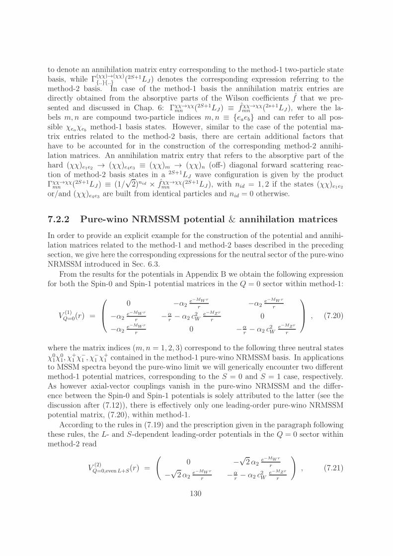
to denote an annihilation matrix entry corresponding to the method-1 two-particle statebasis, while Γ
(χχ)→(χχ).... (2S+1LJ) denotes the corresponding expression referring to the
method-2 basis. In case of the method-1 basis the annihilation matrix entries aredirectly obtained from the absorptive parts of the Wilson coefficients f that we pre-sented and discussed in Chap. 6: Γχχ→χχ
mn (2S+1LJ) ≡ fχχ→χχmn (2s+1LJ ), where the la-
bels m,n are compound two-particle indices m,n ≡ eaeb and can refer to all pos-sible χeaχeb method-1 basis states. However, similar to the case of the potential ma-trix entries related to the method-2 basis, there are certain additional factors thathave to be accounted for in the construction of the corresponding method-2 annihi-lation matrices. An annihilation matrix entry that refers to the absorptive part of thehard (χχ)e1e2 → (χχ)e4e3 ≡ (χχ)m → (χχ)n (off-) diagonal forward scattering reac-tion of method-2 basis states in a 2S+1LJ wave configuration is given by the productΓχχ→χχmn (2S+1LJ) ≡ (1/
√2)nid × fχχ→χχ
mn (2S+1LJ), with nid = 1, 2 if the states (χχ)e1e2or/and (χχ)e4e3 are built from identical particles and nid = 0 otherwise.
7.2.2 Pure-wino NRMSSM potential & annihilation matrices
In order to provide an explicit example for the construction of the potential and annihi-lation matrices related to the method-1 and method-2 bases described in the precedingsection, we give here the corresponding expressions for the neutral sector of the pure-winoNRMSSM introduced in Sec. 6.3.
From the results for the potentials in Appendix B we obtain the following expressionfor both the Spin-0 and Spin-1 potential matrices in the Q = 0 sector within method-1:
V(1)Q=0(r) =
0 −α2e−MWr
r−α2
e−MWr
r
−α2e−MWr
r−α
r− α2 c
2W
e−MZr
r0
−α2e−MWr
r0 −α
r− α2 c
2W
e−MZr
r
, (7.20)
where the matrix indices (m,n = 1, 2, 3) correspond to the following three neutral statesχ01χ
01, χ
+1 χ
−1 , χ
−1 χ
+1 contained in the method-1 pure-wino NRMSSM basis. In applications
to MSSM spectra beyond the pure-wino limit we will generically encounter two differentmethod-1 potential matrices, corresponding to the S = 0 and S = 1 case, respectively.As however axial-vector couplings vanish in the pure-wino NRMSSM and the differ-ence between the Spin-0 and Spin-1 potentials is solely attributed to the latter (see thediscussion after (7.12)), there is effectively only one leading-order pure-wino NRMSSMpotential matrix, (7.20), within method-1.
According to the rules in (7.19) and the prescription given in the paragraph followingthese rules, the L- and S-dependent leading-order potentials in the Q = 0 sector withinmethod-2 read
V(2)Q=0,evenL+S(r) =
(0 −
√2α2
e−MWr
r
−√2α2
e−MWr
r−α
r− α2 c
2W
e−MZr
r
), (7.21)
130
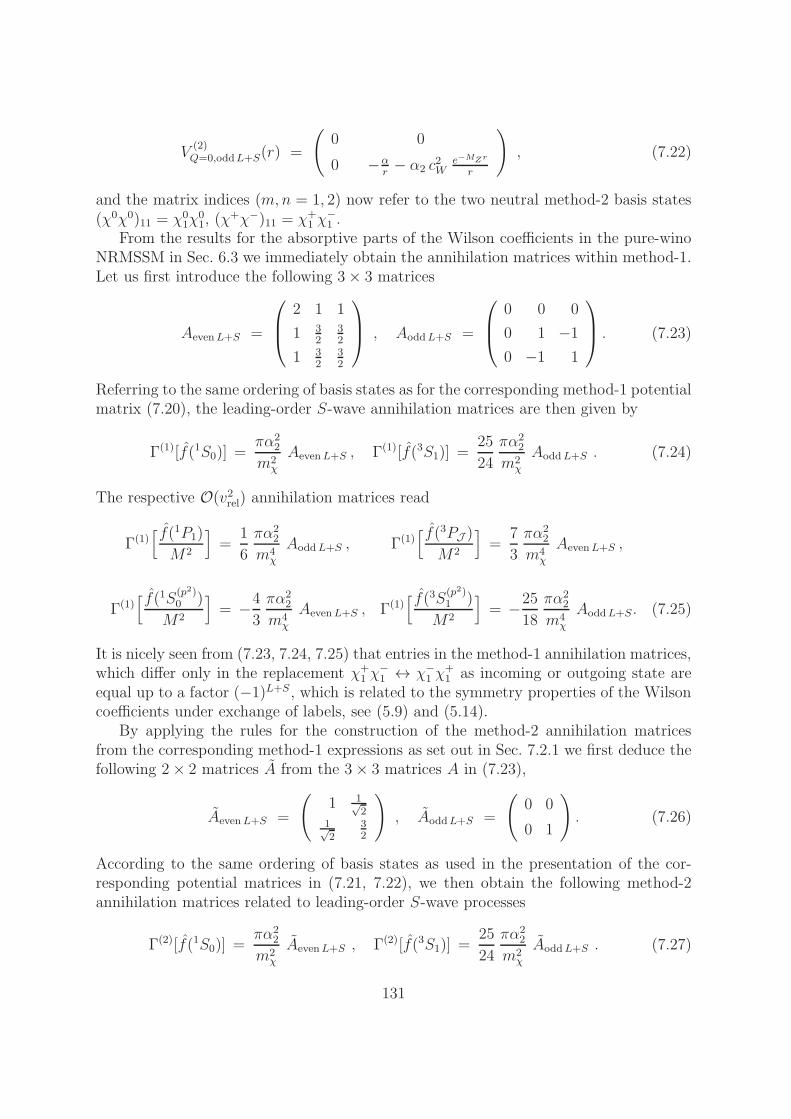
V(2)Q=0,oddL+S(r) =
(0 0
0 −αr− α2 c
2W
e−MZr
r
), (7.22)
and the matrix indices (m,n = 1, 2) now refer to the two neutral method-2 basis states(χ0χ0)11 = χ0
1χ01, (χ
+χ−)11 = χ+1 χ
−1 .
From the results for the absorptive parts of the Wilson coefficients in the pure-winoNRMSSM in Sec. 6.3 we immediately obtain the annihilation matrices within method-1.Let us first introduce the following 3× 3 matrices
AevenL+S =
2 1 1
1 32
32
1 32
32
, AoddL+S =
0 0 0
0 1 −10 −1 1
. (7.23)
Referring to the same ordering of basis states as for the corresponding method-1 potentialmatrix (7.20), the leading-order S-wave annihilation matrices are then given by
Γ(1)[f(1S0)] =πα2
2
m2χ
AevenL+S , Γ(1)[f(3S1)] =25
24
πα22
m2χ
AoddL+S . (7.24)
The respective O(v2rel) annihilation matrices read
Γ(1)[ f(1P1)
M2
]=
1
6
πα22
m4χ
AoddL+S , Γ(1)[ f(3PJ )
M2
]=
7
3
πα22
m4χ
AevenL+S ,
Γ(1)[ f(1S(p2)
0 )
M2
]= −4
3
πα22
m4χ
AevenL+S , Γ(1)[ f(3S(p2)
1 )
M2
]= −25
18
πα22
m4χ
AoddL+S. (7.25)
It is nicely seen from (7.23, 7.24, 7.25) that entries in the method-1 annihilation matrices,which differ only in the replacement χ+
1 χ−1 ↔ χ−
1 χ+1 as incoming or outgoing state are
equal up to a factor (−1)L+S, which is related to the symmetry properties of the Wilsoncoefficients under exchange of labels, see (5.9) and (5.14).
By applying the rules for the construction of the method-2 annihilation matricesfrom the corresponding method-1 expressions as set out in Sec. 7.2.1 we first deduce thefollowing 2× 2 matrices A from the 3× 3 matrices A in (7.23),
AevenL+S =
(1 1√
21√2
32
), AoddL+S =
(0 0
0 1
). (7.26)
According to the same ordering of basis states as used in the presentation of the cor-responding potential matrices in (7.21, 7.22), we then obtain the following method-2annihilation matrices related to leading-order S-wave processes
Γ(2)[f(1S0)] =πα2
2
m2χ
AevenL+S , Γ(2)[f(3S1)] =25
24
πα22
m2χ
AoddL+S . (7.27)
131
The latter results together with (7.21, 7.22) have been presented before in [19, 20]. Theexpressions (7.27) obviously follow from (7.24) by the replacements A → A. In thesame way, replacing A → A in (7.25), the corresponding method-2 O(v2rel) annihilationmatrices are obtained that have not been given before in the literature.
From the results for the pure-wino NRMSSM Wilson coefficients presented in Sec. 6.3and the generic expressions for the potential interactions given in Appendix B, theannihilation and potential matrices in the pure-wino NRMSSM within the remainingQ = ±1,±2 charge sectors can be similarly obtained.
132
Chapter 8
Sommerfeld enhancement
In this chapter we finally come to the rigorous derivation of the non-relativistic χ0/χ±
pair-annihilation cross section including Sommerfeld enhancements within the non-relati-vistic effective theory that we have developed in the preceding Chaps. 5 – 7. The structureof this chapter is as follows. In Sec. 8.1 we start from the annihilation cross section inthe effective theory written in terms of matrix elements of the four-fermion operatorsin δLann and their corresponding Wilson coefficients. From this we derive a convenientform of this central expression given by a sum over products of Sommerfeld enhancementfactors times the corresponding Wilson coefficients encoding the partial-wave dependenthard annihilation rates. The Sommerfeld enhancement factors themselves involve two-particle wave functions in presence of the potential interactions, subject to a certainpartial-wave configuration of the incoming particle pair, as well as corresponding Wilsoncoefficient expressions. In the course of rewriting the cross section we thus provide arefined, rigorous definition of the Sommerfeld enhancement factors first introduced inChap. 2.
At two points in Sec. 8.1 we make use of relations whose detailed derivation is post-poned to later sections. The first point concerns the relation between the operatormatrix elements and two-particle wave functions – appearing in the Sommerfeld en-hancement factors – that we address in Sec. 8.2: we first establish here the connectionbetween the pair-annihilation matrix element and the Green function associated withthe annihilating non-relativistic two-particle state. Elementary scattering theory andthe Lippmann-Schwinger equation subsequently provide the link to the two-particle wavefunctions that are solutions to a corresponding multi-state Schrodinger equation. Even-tually a form of the Sommerfeld enhancement factors of use in practical calculations isderived. As all expressions related to the determination of the Sommerfeld factors andnon-relativistic pair-annihilation cross sections refer to two-particle states, we can makeuse of the method-1 and method-2 two-particle state bases introduced in Sec. 7.2.1.In Sec. 8.3 we therefore rewrite the definition of the Sommerfeld factors in terms ofquantities associated with the one or the other basis. The equivalence of results on theSommerfeld factors derived within the two methods is shown in Appendix. C.
It is worth to stress already here that the final expression for the Sommerfeld en-
133
hancement factors in terms of scattering wave function solutions of a correspondingSchrodinger equation differs slightly with respect to the advanced-guess formula fromChap. 2: if the hermitian potential matrix in the Schrodinger equation is not in ad-dition real-symmetric (Vij = V ∗
ji 6= Vji), the scattering wave function solutions in theSommerfeld factor formula have to be replaced by their complex conjugates with respectto the expression in Chap. 2.1 The steps to numerically determine the Sommerfeld fac-tors for a system of coupled scattering states (χχ)i=1,...,N by solving a multi-componentSchrodinger equation are however easily obtained by adaption of the steps given at theend of Sec. 2.2. It turns out, though, that this method suffers from severe numericalinstabilities in the application to χ0/χ± co-annihilation processes in the general MSSM.The origin of these instabilities is discussed in Sec. 8.4 and an improved method thatallows to resolve the issue is introduced.
The second missing derivation of a relation presupposed in Sec. 8.1 is presented inSec. 8.5, which treats the relation between the matrix elements of the next-to-next-to-leading and the leading-order S-wave four-fermion operators. Eventually, Sec. 8.6contains the description of a method that allows to perturbatively include the effectsfrom heavier neutralino and chargino states that are not part of the NRMSSM in thelast potential loop of ladder-amplitudes prior to the actual pair annihilation.
8.1 Sommerfeld-corrected annihilation rates
In Chap. 5 we have given the generic formula for the inclusive spin-averaged centre-of-mass frame χiχj annihilation cross section in terms of matrix elements of the operatorscontained in δLann, see (5.5). Here we start from this equation and explicitly insert thedimension-6 and dimension-8 four-fermion operators from δLann in the forward-scatteringmatrix element. In this way we obtain the following expression for the inclusive χiχjannihilation cross section in the non-relativistic effective theory:
σχiχj→∑XAXB vrel =
1
4
∑
si, sj
2 ℑ 〈χiχj| δLann|χiχj〉
=1
8
∑
si, sj
(f(1S0) +
δm
Mh1(
1S0) +δm
Mh2(
1S0)
)〈χiχj | O(1S0) |χiχj〉
+
(f(3S1) +
δm
Mh1(
3S1) +δm
Mh2(
3S1)
)〈χiχj | O(3S1) |χiχj〉
+g(1S0)
M2〈χiχj | P(1S0) |χiχj〉 +
g(3S1)
M2〈χiχj| P(3S1) |χiχj〉
1In the analysis of Sommerfeld enhancements in the toy scenarios of Chap. 2 we have considered realpotentials, such that all results discussed in context of these toy models remain valid. In the MSSMapplication, though, we generically encounter potential matrices that are not real-symmetric.
134
+f(1P1)
M2〈χiχj | O(1P1) |χiχj〉 +
3 f(3PJ )
M2〈χiχj| O(3P0) |χiχj〉
+ higher order contributions . (8.1)
Again we use vrel = |~vi − ~vj| to denote the (modulus of the) relative velocity of theannihilating particles χi and χj in their centre-of-mass frame.2 The contributions to(8.1) denoted with ‘higher order’ are related to four-fermion operators in δLann withmass dimension 9 and higher, which are suppressed with respect to the dimension-6 and 8four-fermion operators and therefore safely neglected. The incoming and outgoing statesin (8.1) are non-relativistically normalised, which implies that for the free single-particlemomentum eigenstates of the NRMSSM neutralinos and charginos the normalisation〈 ~p | ~p ′ 〉 = (2π)3δ(3)(~p − ~p ′) holds. We have used a short-hand notation in (8.1), thatallows a concise representation of the different contributions: we suppress the labels onthe four-fermion operators and their corresponding Wilson coefficients that indicate thespecific (off-) diagonal χe1χe2 → χe4χe3 scattering reaction to which these quantitiesrefer. In addition the sum symbol over all such (off-) diagonal χχ → χχ reactions,compatible with the charge of the incoming χiχj state, has been omitted. Written infull form the first term in (8.1) for instance reads
1
8
∑
si, sj
∑
χχ→χχ
fχχ→χχe1e2e4e3(
1S0) 〈χiχj | Oχχ→χχe4e3e2e1(
1S0) |χiχj〉 . (8.2)
In the following we will always omit the sum symbol∑
χχ→χχ and imply summation overrepeated indices ei if those appear in an expression. Let us further recall from Sec. 5.2.2that the quantitiesM , δm and δm that come with the dimension-8 four-fermion operatorsin (8.1) denote χe1χe2 → χe4χe3 process-specific quantities.
In order to obtain the second equality in (8.1) we used the fact that
ℑ[f(2S+1LJ) 〈χiχj| O(2S+1LJ) |χiχj〉
]= f(2S+1LJ) 〈χiχj | O(2S+1LJ) |χiχj〉 , (8.3)
which follows from (6.5) and (6.6). A similar relation obviously holds for the next-to-next-to-leading order S-wave operators P(2S+1SS). The forward-scattering matrixelements of the three spin S = 1 P -wave operators, 〈χiχj|O(3PJ=0,1,2)|χiχj〉, agree apartfrom simple spin-weighted factors, as long as only leading-order potential interactionsthat do not change the spin and orbital angular momentum of the incoming χiχj stateare considered in the calculation. Since our analysis is restricted to leading-order po-tentials we have therefore already expressed the spin S = 1 P -wave contributions to the
2As already noted in context of (5.5) (see footnote 4 in Chap. 5) also here we abuse notationto make contact with the common notation used in quarkonium annihilations and write in (8.1)the matrix elements of the operators δLann, O(2S+1LJ) and P(2S+1LJ) instead of the correspond-ing forward-scattering amplitudes. The proper way to write the relation (8.1) would involve theconfiguration-space integrated quantities,
∫d4x δLann,
∫d4xO(2S+1LJ) and
∫d4xP(2S+1LJ) in the
forward-scattering matrix elements on the right-hand side instead of the sole operators. The additionalfactors (2π)4 δ(4)(pinitial − pfinal) that then arise when evaluating the matrix elements should howevernot be included in the relation to the cross section (8.1).
135

annihilation cross section in (8.1) in terms of the matrix element of the operator O(3P0)multiplied by f(3PJ ), the appropriate spin-weighted sum of the three spin-1 P -waveWilson coefficients introduced in (6.29).
Note that we immediately obtain the exclusive tree-level annihilation cross sections(6.22) from (8.1), when the matrix elements are evaluated for the perturbative case(neglecting long-range potential interactions contained in Lpot) and when the Wilsoncoefficients are determined at O(α2
i ). At this order infrared divergences are absent suchthat (8.1) applies separately for each exclusive final state XAXB. Consequently, as wehave explicitly used in Chap. 6, the contributions to the Wilson coefficients f , g and hifrom χχ→ XAXB → χχ reactions can be given separately and therefore allow to obtainthe non-relativistic expansion of the exclusive χiχj → XAXB tree-level annihilation crosssection including O(v2rel) contributions.
Eventually we want to rewrite (8.1) such that the non-relativistic expansion of theχiχj pair-annihilation cross section is expressed in terms of a sum over products of Wilsoncoefficients – encoding the short-distance annihilations – and their corresponding partial-wave dependent Sommerfeld enhancement factors, which are related to the long-rangeeffects. To this end we proceed in three steps. First we express the matrix elements of theoperators in terms of non-relativistic wave-functions and their derivatives evaluated atthe origin, a procedure well known from quarkonium physics. Subsequently we providethe definition of the Sommerfeld enhancement factors in terms of Wilson coefficients andthe non-relativistic wave-functions, which refines the corresponding definition in Chap. 2.From this we finally obtain the desired expression for the χiχj pair-annihilation crosssection, that explicitly involves the Sommerfeld enhancement factors.
In the first step we start from the matrix elements of the four-fermion operators andinsert the operator |0〉〈0| that projects onto the NRMSSM vacuum state, the Fock spacestate that involves no neutralinos and charginos. For instance, the matrix element of thedimension-6 operator O(1S0) is with this insertion written as
〈χiχj | Oχχ→χχe4e3e2e1(
1S0) |χiχj〉 = 〈χiχj |χ†e4χce3|0〉〈0|χ
c †e2χe1 |χiχj〉
=[〈ξc†j ξi〉
(ψ
(0,0)e4e3,ij
+ ψ(0,0)e3e4,ij
)]∗〈ξc†j ξi〉
(ψ
(0,0)e1e2,ij
+ ψ(0,0)e2e1,ij
). (8.4)
Note that the relation in the first line is exact at the level of terms that we include inLkin+Lpot. With the second equality in (8.4) we define ψ
(L=0,S=0)eaeb,ij
, the χeaχeb-componentof a scattering wave function related to the incoming χiχj state with centre-of-massenergy
√s, orbital angular momentum L = 0 and total spin S = 0, evaluated for
zero relative distance and normalised to the free scattering solution. The quantitiesξi, ξj denote the two-component Pauli spinors of the incoming particles and we use thenotation 〈 .. 〉 to indicate the trace in spin space. The relation between the matrix element〈0|χc †e2χe1 |χiχj〉 and the wave functions in (8.4) is generalised in the following way to thecase of 2S+1LJ partial-wave reactions:
〈0|χc†e2ΓK[− i
2
←→∂]χe1|χiχj〉 = 〈ξ
c†j Γξi〉K[~p ]
(ψ
(L,S)e1e2, ij
+ (−1)L+S ψ(L,S)e2e1, ij
), (8.5)
136
where Γ = 12×2 in case of total spin S = 0 and Γ = ~σ for S = 1. Further, K denotesa polynomial in relative momentum ~p = ~pij of the incoming χiχj pair (or, accordingly,derivatives in position space) corresponding to a given angular momentum L. Generi-
cally, the multi-component wave-function ~ψ(L,S)ij encodes the effect of all (off-) diagonal
potential interactions that involve the incoming non-relativistic χiχj pair in a 2S+1LJpartial-wave state as well as all possible further (intermediate) neutralino and charginoNRMSSM two-particle states with the same charge and within the same partial-waveconfiguration. In the perturbative case, where the potential interactions in Lpot are ne-
glected, the wave functions reduce to ψ(L,S)eaeb,ij
→ δeai δebj. This can be checked explicitlyby direct calculation of the matrix elements of the operators in the perturbative case,which in particular leads to the result for the tree-level annihilation cross section in(6.22). The explicit determination of the wave functions from the matrix elements onthe left-hand side in (8.5) is postponed to Sec. 8.2. Here we use the relation (8.5) toexpress the spin-averaged annihilation cross section (8.1) in terms of the non-relativisticwave functions,
σχiχj→∑XAXB vrel
=[ψ
(0,0)e4e3, ij
]∗(f(1S0) +
δm
Mh1(
1S0) +δm
Mh2(
1S0) + gκ(1S0)
)ψ
(0,0)e1e2, ij
+ 3[ψ
(0,1)e4e3, ij
]∗(f(3S1) +
δm
Mh1(
3S1) +δm
Mh2(
3S1) + gκ(3S1)
)ψ
(0,1)e1e2, ij
+ ~p 2ij
[ψ
(1,0)e4e3, ij
]∗ f(1P1)
M2ψ
(1,0)e1e2, ij
+ ~p 2ij
[ψ
(1,1)e4e3, ij
]∗ f(3PJ )
M2ψ
(1,1)e1e2, ij
, (8.6)
where we have used the spin sums
1
2
∑
si,sj
〈ξc†j ξi〉 〈ξc†j ξi〉∗ = 1 ,1
2
∑
si,sj
〈ξc†j σkξi〉 〈ξc†j σℓξi〉∗ = δkℓ , (8.7)
as well as the symmetry properties (5.9, 5.14) of the Wilson coefficients. The relativemomentum ~pij of the two non-relativistic particles χi and χj in the χiχj two-particlestate is related to the available centre-of-mass energy
√s by
~p 2ij = 2µij (
√s−Mij) + O(~p 4
ij ) , (8.8)
with µij the reduced and Mij the total mass of the two-particle system. In addition weuse in (8.6) the following relation between the matrix elements of the next-to-next-to-leading and the leading-order S-wave operators P(2S+1SS) and O(2S+1SS),
g(2S+1SS)
M2〈χiχj | P(2S+1SS) |χiχj〉 = gκ(
2S+1SS) 〈χiχj | O(2S+1SS) |χiχj〉 , (8.9)
with
gκ e′1e′2e′4e′3(2S+1SS) =
ge1e2e4e3(2S+1SS)
2M2
(κ∗e1e2,e′1e′2δe4e3,e
′4e
′3+ δe1e2,e′1e′2κe4e3,e′4e′3
)(8.10)
137

and the parameter κ defined as
κe1e2,e′1e′2 = ~p 2e1e2
δe1e2,e′1e′2 + 2µe1e2α2
∑
a
mφa c(a)e1e2,e′1e
′2. (8.11)
The sum in the second term in (8.11) runs over all potential scattering reactions χe′1χe′2 →χe1χe2 arising from φa-mediator exchange. The corresponding coefficients c
(a)e1e2,e′1e
′2are
collected in Tab. B.1. The definition for the relative momentum ~p 2e1e2
in (8.11) followsfrom (8.8). The derivation of relation (8.9) is postponed to Sec. 8.5. Let us howevernote here, that the simpler form 〈χχ| P(2S+1SS) |χχ〉 = ~p 2 〈χχ| O(2S+1SS) |χχ〉 familiarfrom NRQCD applications to heavy quarkonium is obtained from (8.9 – 8.11), whenthe theory contains just one single two-particle state and the exchanged bosons φa aremassless.
As second step in our derivation of a χiχj cross section formula involving products ofSommerfeld enhancement factors and Wilson coefficients, we provide now the definitionof the Sommerfeld enhancement factor for an incoming χiχj state with centre-of-massenergy
√s, spin S and orbital angular momentum L. The enhancement factor is asso-
ciated with Wilson coefficients (or suitable combinations of Wilson coefficients) f , thatencode the corresponding short-distance annihilations subject to the given total spin Sand orbital angular momentum L, and defined by the ratio
Sij [f(2S+1LJ)] =
[ψ
(L,S)e4e3, ij
]∗fχχ→χχe1e2e4e3(
2S+1LJ )ψ(L,S)e1e2, ij
fχχ→χχijij(
2S+1LJ )|LO. (8.12)
This definition has to be understood such that according to the expressions in the expan-sion of the cross section (8.6), for instance, the combinations f(1P1)/M
2 and f(3PJ )/M2
appear as arguments of the corresponding Sij . In case of leading-order S-waves the argu-
ments are simply given by f(1S0) and f(3S1). It is worth to recall at this point that the
mass scale M that comes with the Wilson coefficients of dimension-8 operators in δLann
derives from the masses of the particles χei=1,...,4to which the respective Wilson coefficient
f refers. With the subscript “LO” in the denominator of (8.12) we indicate that only thatcontribution to f(2S+1LJ) that is leading order in the coupling α2, O(α2
2), should be keptin the corresponding expressions. As far as our application is concerned, this prescrip-tion is only relevant to us for the case of enhancement factors associated with next-to-next-to-leading order S-wave annihilations, Sij [gκ(
2S+1SS)], where we have to set the α2
proportional term in κ to zero, so that gχχ→χχκijij(
2S+1SS)|LO = ~p 2ij/M
2ij g
χχ→χχijij(
2S+1SS).
However note that definition (8.12) generically allows to incorporate the higher-order(hard) radiative corrections to the short-distance part of the annihilation into the Som-merfeld factor. Though not explicitly indicated in (8.12) it is important to note that theSommerfeld enhancement factors depend on the available centre-of-mass energy
√s or,
equivalently, the relative velocity vrel of the incoming χiχj state.As third and final step, using the definition (8.12), we parametrise the non-relativistic
expansion of the inclusive χiχj pair-annihilation cross section in (8.1) in terms of Som-
138
merfeld enhancement factors and Wilson coefficients:
σχiχj→∑XAXB vrel = Sij [fh(
1S0)] fχχ→χχijij(
1S0) + Sij[fh(3S1)] 3 f
χχ→χχijij(
3S1)
+~p 2ij
M2ij
(Sij[gκ(
1S0)] gχχ→χχijij(
1S0) + Sij [gκ(3S1)] 3 g
χχ→χχijij(
3S1)
+ Sij
[ f(1P1)
M2
]fχχ→χχijij(
1P1) + Sij
[ f(3PJ )
M2
]fχχ→χχijij(
3PJ )), (8.13)
where in addition to the spin-weighted sum f(3PJ ) of spin S = 1 P -wave Wilson coeffi-cients defined in (6.29), we introduced the following combinations of Wilson coefficients
fh(1S0) = f(1S0) +
δm
Mh1(
1S0) +δm
Mh2(
1S0) ,
fh(3S1) = f(3S1) +
δm
Mh1(
3S1) +δm
Mh2(
3S1) . (8.14)
The non-relativistic expansion of the inclusive χiχj tree-level annihilation cross section isrecovered from (8.13) by setting all Sommerfeld enhancement factors to one. In this casethe cross section formula contains only those Wilson coefficients that refer to diagonalχiχj → χiχj reactions. Wilson coefficients related to off-diagonal rates – in particular
the coefficients hi=1,2 that vanish for diagonal reactions – can only enter the Sommerfeld
enhancement factors. This is why the symbols fh appear only as arguments of the factorsSij in (8.13).
8.2 NR matrix-elements & the Schrodinger equation
In this section we provide the missing derivation of the relation between the matrixelements and wave functions in (8.5). We proceed in three steps: first a relation betweenthe matrix elements and corresponding momentum space two-particle Green functionsis established. Second, we move to the corresponding coordinate-space Green functionsand, third, use elementary scattering theory to obtain an expression involving scatteringwave functions instead of the Green functions.
The non-relativistic matrix element in (8.5) systematically includes long-range po-tential interactions, which cannot be treated perturbatively but require a resummationup to all orders. We have noted in Chap. 2 that the corresponding contributions to thematrix element are obtained from a resummation of the potential region contributionsto ladder diagrams such as Fig. 8.1. To extract the relevant expressions from the fulltheory ladder diagrams we can perform similar replacements as in Sec. 2.1, (2.5, 2.6),for the (ladder bar) fermion and (ladder rung) boson propagators. Let us recall howeverthat compared to Chap. 2 we consider here the case of several nearly mass degeneratefermion states, where the corresponding mass differences shall be of the same order asthe non-relativistic kinetic energy of the external states. We write the on-shell momenta
139
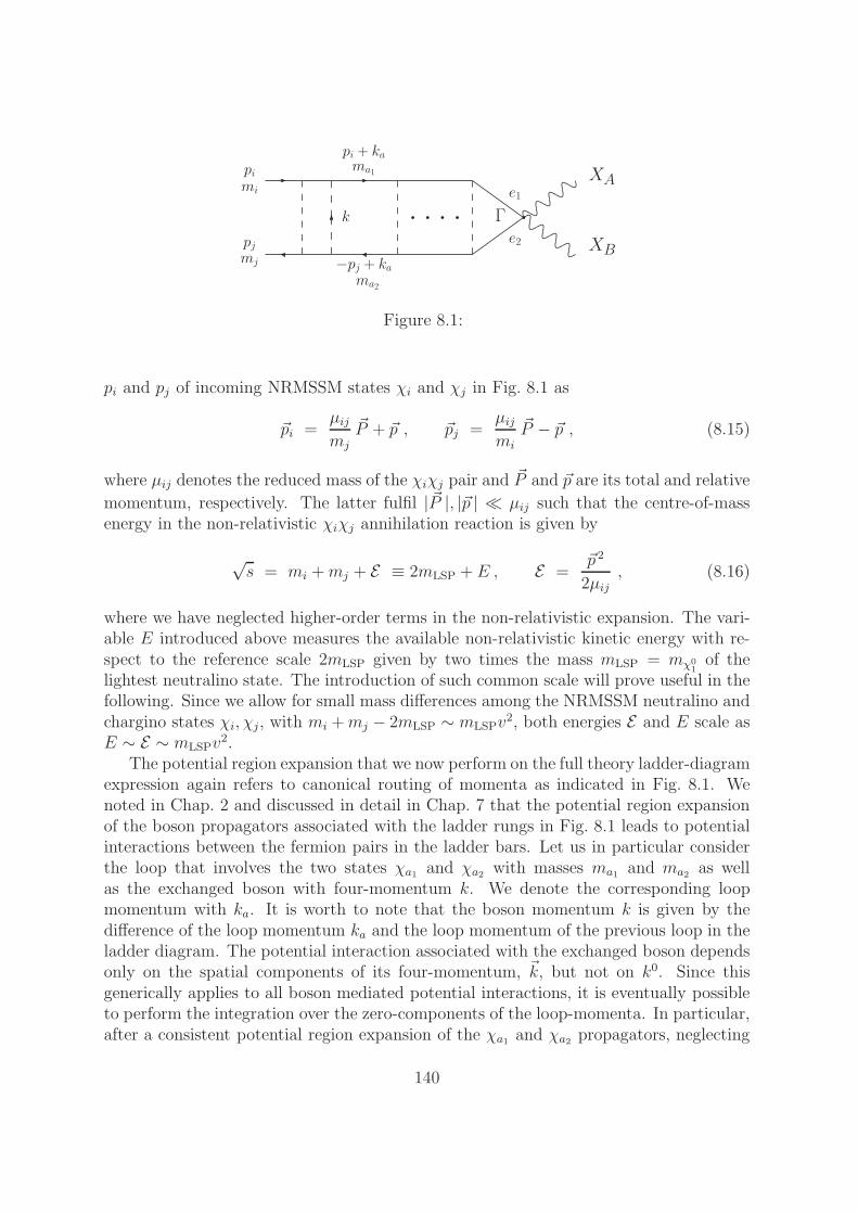
pi + kama1pi
mi
pjmj −pj + ka
ma2
k
XA
XB
Γ
e1
e2
Figure 8.1:
pi and pj of incoming NRMSSM states χi and χj in Fig. 8.1 as
~pi =µijmj
~P + ~p , ~pj =µijmi
~P − ~p , (8.15)
where µij denotes the reduced mass of the χiχj pair and ~P and ~p are its total and relative
momentum, respectively. The latter fulfil |~P |, |~p | ≪ µij such that the centre-of-massenergy in the non-relativistic χiχj annihilation reaction is given by
√s = mi +mj + E ≡ 2mLSP + E , E =
~p 2
2µij, (8.16)
where we have neglected higher-order terms in the non-relativistic expansion. The vari-able E introduced above measures the available non-relativistic kinetic energy with re-spect to the reference scale 2mLSP given by two times the mass mLSP = mχ0
1of the
lightest neutralino state. The introduction of such common scale will prove useful in thefollowing. Since we allow for small mass differences among the NRMSSM neutralino andchargino states χi, χj, with mi +mj − 2mLSP ∼ mLSPv
2, both energies E and E scale asE ∼ E ∼ mLSPv
2.The potential region expansion that we now perform on the full theory ladder-diagram
expression again refers to canonical routing of momenta as indicated in Fig. 8.1. Wenoted in Chap. 2 and discussed in detail in Chap. 7 that the potential region expansionof the boson propagators associated with the ladder rungs in Fig. 8.1 leads to potentialinteractions between the fermion pairs in the ladder bars. Let us in particular considerthe loop that involves the two states χa1 and χa2 with masses ma1 and ma2 as wellas the exchanged boson with four-momentum k. We denote the corresponding loopmomentum with ka. It is worth to note that the boson momentum k is given by thedifference of the loop momentum ka and the loop momentum of the previous loop in theladder diagram. The potential interaction associated with the exchanged boson dependsonly on the spatial components of its four-momentum, ~k, but not on k0. Since thisgenerically applies to all boson mediated potential interactions, it is eventually possibleto perform the integration over the zero-components of the loop-momenta. In particular,after a consistent potential region expansion of the χa1 and χa2 propagators, neglecting
140
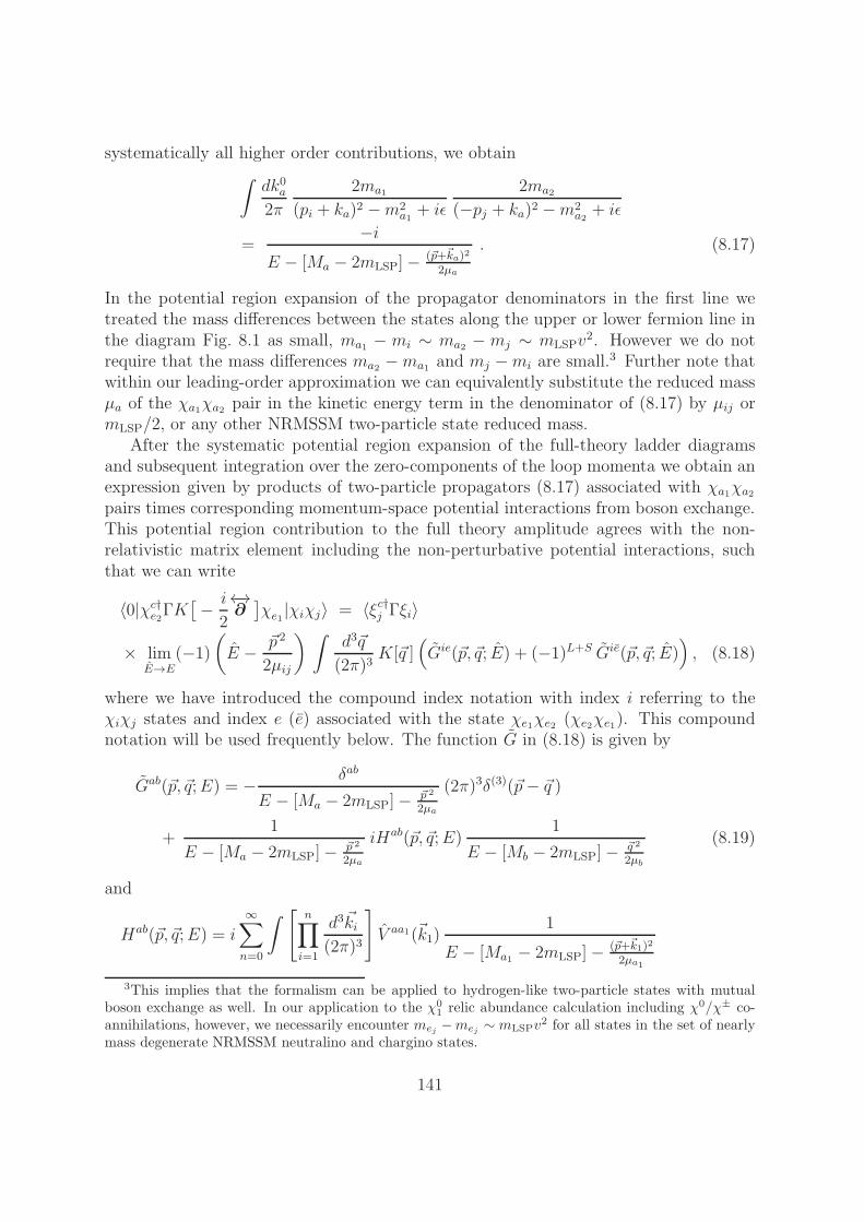
systematically all higher order contributions, we obtain∫dk0a2π
2ma1
(pi + ka)2 −m2a1+ iǫ
2ma2
(−pj + ka)2 −m2a2+ iǫ
=−i
E − [Ma − 2mLSP]− (~p+~ka)2
2µa
. (8.17)
In the potential region expansion of the propagator denominators in the first line wetreated the mass differences between the states along the upper or lower fermion line inthe diagram Fig. 8.1 as small, ma1 − mi ∼ ma2 − mj ∼ mLSPv
2. However we do notrequire that the mass differences ma2 −ma1 and mj −mi are small.3 Further note thatwithin our leading-order approximation we can equivalently substitute the reduced massµa of the χa1χa2 pair in the kinetic energy term in the denominator of (8.17) by µij ormLSP/2, or any other NRMSSM two-particle state reduced mass.
After the systematic potential region expansion of the full-theory ladder diagramsand subsequent integration over the zero-components of the loop momenta we obtain anexpression given by products of two-particle propagators (8.17) associated with χa1χa2pairs times corresponding momentum-space potential interactions from boson exchange.This potential region contribution to the full theory amplitude agrees with the non-relativistic matrix element including the non-perturbative potential interactions, suchthat we can write
〈0|χc†e2ΓK[− i
2
←→∂]χe1 |χiχj〉 = 〈ξc†j Γξi〉
× limE→E
(−1)(E − ~p 2
2µij
) ∫d3~q
(2π)3K[~q ]
(Gie(~p, ~q; E) + (−1)L+S Gie(~p, ~q; E)
), (8.18)
where we have introduced the compound index notation with index i referring to theχiχj states and index e (e) associated with the state χe1χe2 (χe2χe1). This compoundnotation will be used frequently below. The function G in (8.18) is given by
Gab(~p, ~q;E) = − δab
E − [Ma − 2mLSP]− ~p 2
2µa
(2π)3δ(3)(~p− ~q )
+1
E − [Ma − 2mLSP]− ~p 2
2µa
iHab(~p, ~q;E)1
E − [Mb − 2mLSP]− ~q 2
2µb
(8.19)
and
Hab(~p, ~q;E) = i
∞∑
n=0
∫ [ n∏
i=1
d3~ki(2π)3
]V aa1(~k1)
1
E − [Ma1 − 2mLSP]− (~p+~k1)2
2µa1
3This implies that the formalism can be applied to hydrogen-like two-particle states with mutualboson exchange as well. In our application to the χ0
1 relic abundance calculation including χ0/χ± co-annihilations, however, we necessarily encounter mej −mej ∼ mLSPv
2 for all states in the set of nearlymass degenerate NRMSSM neutralino and chargino states.
141
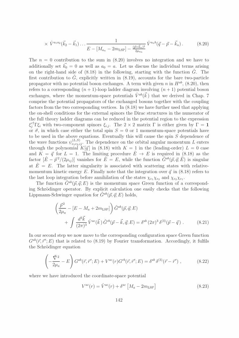
× V a1a2(~k2 − ~k1) . . .1
E − [Man − 2mLSP]− (~p+~kn)2
2µan
V anb(~q − ~p− ~kn) . (8.20)
The n = 0 contribution to the sum in (8.20) involves no integration and we have to
additionally set ~k0 = 0 as well as a0 = a. Let us discuss the individual terms arisingon the right-hand side of (8.18) in the following, starting with the function G. Thefirst contribution to G, explicitly written in (8.19), accounts for the bare two-particlepropagator with no potential boson exchanges. A term with given n in Hab, (8.20), thenrefers to a corresponding (n + 1)-loop ladder diagram involving (n+ 1) potential boson
exchanges, where the momentum-space potentials V ab(~k ) that we derived in Chap. 7comprise the potential propagators of the exchanged bosons together with the couplingfactors from the two corresponding vertices. In (8.18) we have further used that applyingthe on-shell conditions for the external spinors the Dirac structures in the numerator ofthe full theory ladder diagrams can be reduced in the potential region to the expressionξc†j Γξi with two-component spinors ξi,j. The 2 × 2 matrix Γ is either given by Γ = 1or ~σ, in which case either the total spin S = 0 or 1 momentum-space potentials haveto be used in the above equations. Eventually this will cause the spin S dependence ofthe wave functions ψ
(L,S)e1e2,ij
. The dependence on the orbital angular momentum L entersthrough the polynomial K[~q ] in (8.18) with K = 1 in the (leading-order) L = 0 caseand K = ~q for L = 1. The limiting procedure E → E is required in (8.18) as thefactor [E − ~p 2/(2µij)] vanishes for E = E, while the function Gab(~p, ~q; E) is singular
at E = E. The latter singularity is associated with scattering states with relative-momentum kinetic energy E. Finally note that the integration over ~q in (8.18) refers tothe last loop integration before annihilation of the states χe1χe2 and χe2χe1.
The function Gab(~p, ~q;E) is the momentum space Green function of a correspond-ing Schrodinger operator. By explicit calculation one easily checks that the followingLippmann-Schwinger equation for Gab(~p, ~q;E) holds,
(~p 2
2µa− [E −Ma + 2mLSP]
)Gab(~p, ~q;E)
+
∫d3~k
(2π)3V ac(~k ) Gcb(~p− ~k, ~q;E) = δab (2π)3 δ(3)(~p− ~q ) . (8.21)
In our second step we now move to the corresponding configuration space Green functionGab(~r, ~r ′;E) that is related to (8.19) by Fourier transformation. Accordingly, it fulfilsthe Schrodinger equation
(−~∇ 2
2µa− E
)Gab(~r, ~r ′;E) + V ac(r)Gcb(~r, ~r ′;E) = δab δ(3)(~r − ~r ′) , (8.22)
where we have introduced the coordinate-space potential
V ac(r) = V ac(r) + δac[Ma − 2mLSP
](8.23)
142
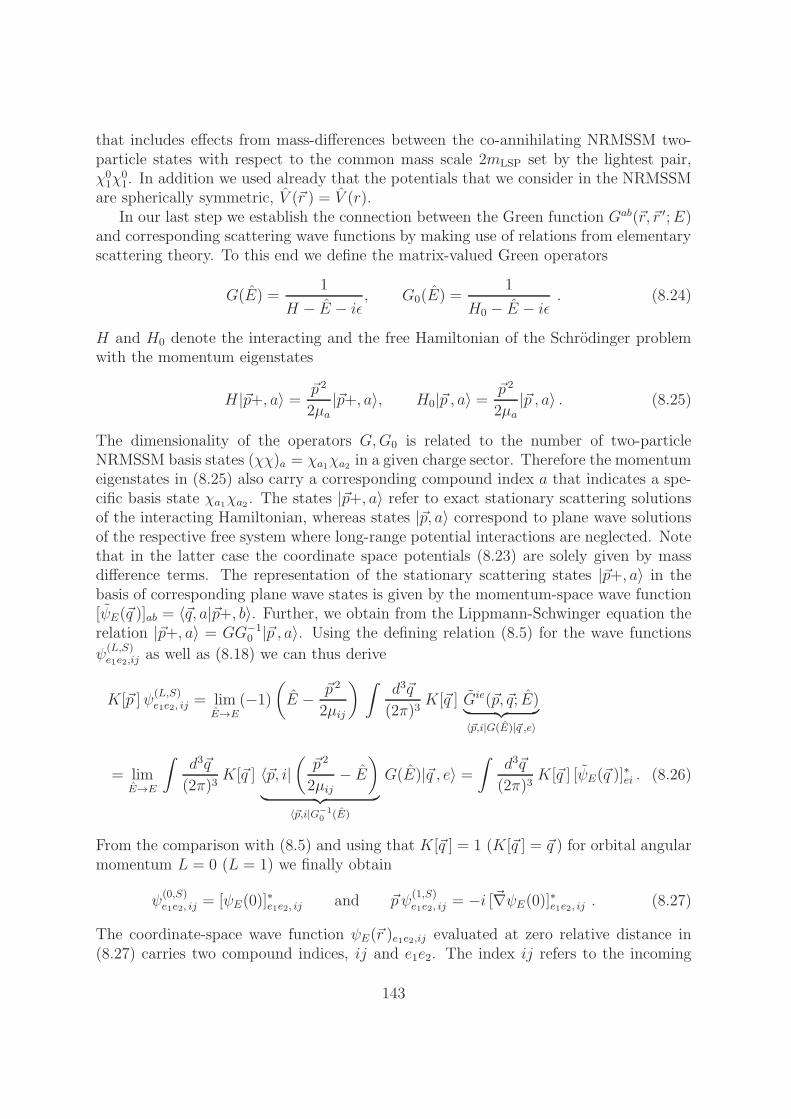
that includes effects from mass-differences between the co-annihilating NRMSSM two-particle states with respect to the common mass scale 2mLSP set by the lightest pair,χ01χ
01. In addition we used already that the potentials that we consider in the NRMSSM
are spherically symmetric, V (~r ) = V (r).In our last step we establish the connection between the Green function Gab(~r, ~r ′;E)
and corresponding scattering wave functions by making use of relations from elementaryscattering theory. To this end we define the matrix-valued Green operators
G(E) =1
H − E − iǫ, G0(E) =
1
H0 − E − iǫ. (8.24)
H and H0 denote the interacting and the free Hamiltonian of the Schrodinger problemwith the momentum eigenstates
H|~p+, a〉 = ~p 2
2µa|~p+, a〉, H0|~p , a〉 =
~p 2
2µa|~p , a〉 . (8.25)
The dimensionality of the operators G,G0 is related to the number of two-particleNRMSSM basis states (χχ)a = χa1χa2 in a given charge sector. Therefore the momentumeigenstates in (8.25) also carry a corresponding compound index a that indicates a spe-cific basis state χa1χa2 . The states |~p+, a〉 refer to exact stationary scattering solutionsof the interacting Hamiltonian, whereas states |~p, a〉 correspond to plane wave solutionsof the respective free system where long-range potential interactions are neglected. Notethat in the latter case the coordinate space potentials (8.23) are solely given by massdifference terms. The representation of the stationary scattering states |~p+, a〉 in thebasis of corresponding plane wave states is given by the momentum-space wave function[ψE(~q )]ab = 〈~q, a|~p+, b〉. Further, we obtain from the Lippmann-Schwinger equation therelation |~p+, a〉 = GG−1
0 |~p , a〉. Using the defining relation (8.5) for the wave functions
ψ(L,S)e1e2,ij
as well as (8.18) we can thus derive
K[~p ]ψ(L,S)e1e2, ij
= limE→E
(−1)(E − ~p 2
2µij
) ∫d3~q
(2π)3K[~q ] Gie(~p, ~q; E)︸ ︷︷ ︸
〈~p,i|G(E)|~q ,e〉
= limE→E
∫d3~q
(2π)3K[~q ] 〈~p, i|
(~p 2
2µij− E
)
︸ ︷︷ ︸〈~p,i|G−1
0 (E)
G(E)|~q , e〉 =∫
d3~q
(2π)3K[~q ] [ψE(~q )]
∗ei . (8.26)
From the comparison with (8.5) and using that K[~q ] = 1 (K[~q ] = ~q ) for orbital angularmomentum L = 0 (L = 1) we finally obtain
ψ(0,S)e1e2, ij
= [ψE(0)]∗e1e2, ij
and ~p ψ(1,S)e1e2, ij
= −i [~∇ψE(0)]∗e1e2, ij . (8.27)
The coordinate-space wave function ψE(~r )e1e2,ij evaluated at zero relative distance in(8.27) carries two compound indices, ij and e1e2. The index ij refers to the incoming
143
χiχj pair described by the incoming plane wave two-particle state |~p, i〉 with kineticenergy E in the centre-of-mass frame of the annihilation reaction. Consequently, thecompound index e1e2 indicates the component of the full scattering wave function withincoming χiχj pair that refers to the χe1χe2 state. The latter e1e2 component is picked
out (at ~r = 0) by the annihilation operator that defines ψ(L,S)e1e2,ij
through (8.5). Thecoordinate space scattering wave functions [ψE(~r )]a,ij are obtained as solutions of thematrix Schrodinger equation
([−~∇ 2
2µa−E
]δab + V ab(r)
)[ψE(~r )]b,ij = 0 (8.28)
with the matrix-valued coordinate-space potentials obtained from (8.23). The initialcondition for a solution ψE(~r )b,ij has to be chosen such that the asymptotic incomingstate refers to the χiχj pair. Due to our assumption on the mass splittings betweenthe NRMSSM states to be of O(mLSPv
2), we can replace the reduced mass µa in (8.28)by the reduced mass mLSP/2 in the lightest NRMSSM two-particle system χ0
1χ01. The
difference is an O(v2) effect which we consistently neglect in the part of the annihilationrates that is associated with the long-range effects. Let us recall that we have performedthe same approximation in Sec. 2.2, see (2.9, 2.11) and the corresponding discussiontherein. Consequently, we have to determine within our non-relativistic approximationthe wave functions [ψE(~r )]a,ij that are solutions of the Schrodinger equation
([−
~∇ 2
mLSP
−E]δab + V ab(r)
)[ψE(~r )]b,ij = 0 , (8.29)
with initial conditions chosen such that [ψE(~r )]b,ij refers to the asymptotic incomingstates χiχj.
It is important to note that the relation among the wave functions ψ(L,S)e1e2,ij
and[ψE(0)]e1e2,ij in (8.27) involves a complex conjugation. Using (8.27) in the refined defini-tion of the Sommerfeld factor in (8.12), we therefore conclude that the advanced-guessSommerfeld enhancement formula from Chap. 2, (2.8, 2.33), was correct up to complexconjugation of the scattering wave function appearing therein.4 While this has con-sequences for the enhancement formulae, we can however directly use all results fromChap. 2 that are related to the scattering solution wave functions [ψE(~r )]b,i.
5 Taking
4Let us mention that the appearance of the complex conjugated scattering wave function [ψE(~q )]∗ei
in (8.26) is related to the convention used for the left and right states in the definition of the Greenfunction (8.19). When using the opposite convention we would end up with a wave function [ψE(~q )]eiin (8.26), but with V ba instead of V ab in the corresponding Schrodinger equation (8.29). Note that thesolutions ψE(~r ) and [ψE(~r )]
∗ are identical for real-symmetric potentials, such that the correct result forthe Sommerfeld enhancement factor would be obtained even if the conventions for the Green functionand the potential were not consistently taken care of: this is the case for the toy model results inChap. 2. In the MSSM, however, we encounter in general complex-hermitian potential matrices.
5Within the NRMSSM we have established the convention to use lowercase letters for the compound
144
the normalisation convention for ψ(L,S) noted in context of its definition in (8.5) intoaccount, we derive the following relation from (2.31) and (2.32),
ψ(L,S)e,i =
(2L+ 1)!!
(L+ 1)![χ
(L+1)L (0)]∗eb
[M−1L ]∗bi
kL+1i
. (8.30)
χL denotes the regular L-th partial wave solution to the radial Schrodinger equationrelated to (8.29). The wave numbers ki are given by
ki =√mLSP (E + iǫ− δMi) , (8.31)
where δMi =Mi−2mLSP is the mass splitting of the two-particle state (χχ)i with respectto the state χ0
1χ01. As E measures the non-relativistic kinetic energy with respect to the
scale 2mLSP, the definition (8.31) agrees with (2.16). Finally, the definition of ML isobtained from (2.20). Using (2.42), we eventually obtain the relation
ψ(L,S)e1e2,ij
= i−L (2L− 1)!![T TL ]eikLi
, (8.32)
which expresses ψ(L,S) in terms of the transpose of the coefficient matrix TL associatedwith the large r behaviour of the singular radial solutions, see (2.37).
With these preparations we can rewrite the Sommerfeld enhancement factor (8.12)using the matrix TL as
Si[f(2S+1LJ)] =
((2L− 1)!!
kLi
)2[T ∗L]ie′ f
χχ→χχee′ (2S+1LJ ) [T
TL ]ei
fχχ→χχii (2S+1LJ)|LO
=
((2L− 1)!!
kLi
)2[TL]ie f
χχ→χχee′ (2S+1LJ ) [T
†L]e′i
fχχ→χχii (2S+1LJ)|LO
. (8.33)
In the second line we have just reordered the factors in the numerator. With the latterrewriting we arrive at our final expression for the Sommerfeld enhancement factors, thatallows for the following clear reading from left to right: The ie component of the firstmatrix factor in the numerator, [TL]ie, is associated with the e-state component of the (Lpartial-wave) scattering wave function at the origin that refers to incoming two-particlestate i. This matrix component is multiplied with the Wilson coefficient fee′ encodingthe absorptive part of the forward scattering reactions from state e to state e′. Finally,the factor [T †
L]e′i is associated with the complex conjugate of the e′ states’ component ofthe wave function referring to incoming state i. This notation has the advantage that all
indices denoting the two particle channels, (χχ)i, opposed to capital letters, (χχ)I , in Chap. 2. In thelatter chapter the notation ψ(~r )JI was used to refer to scattering solutions of a corresponding matrixSchrodinger equation with incoming two-particle state (χχ)I , where the label J used to indicate thecomponent of the wave function related to the two-particle state (χχ)J . Here, the same quantity isdenoted with [ψE(~r )]j,i, where according to our notation convention the compound index i is associatedwith the incoming pair (χχ)i and the index j picks the component corresponding to the (χχ)j state.
145
quantities appear in the same order, from left to right, as in the diagrammatic picturesfor the corresponding processes such as Fig. 5.1. The matrix TL can be determined byfollowing the first two steps proposed at the end of Sec. 2.2. In Sec. 8.4 we discuss theissue of numerical instabilities associated with the strategy of Sec. 2.2 and present animproved method for solving the problem. Before, we replace in the next section theWilson coefficients that appear in the definition (8.12) and in the conveniently rewrittenform (8.33) of the Sommerfeld enhancement factors by appropriate annihilation matricesintroduced in Sec. 7.2.
8.3 Sommerfeld factors in the method-1 and 2 bases
In Sec. 7.2 we have argued that pair-annihilation processes of non-relativistic neutralinoand chargino states including long-range potential interactions can be described by two-particle propagators (as explicitly seen in the previous section), two-particle state poten-tial interactions and the final hard two-particle annihilation reaction, such that the useof a two-particle states basis is obvious. Correspondingly we introduced potential andannihilation matrices subject to the so-called method-1 or method-2 two-particle statebases, see Sec. 7.2.1. Here we come back to these bases and present a form of the Som-merfeld enhancement factors defined in (8.12), that involves the matrix representationsof potential scattering and annihilation reactions introduced in Sec. 7.2.
Let us first note that the derivation in Sec. 8.1 – and therefore in particular thedefinition of the Sommerfeld enhancement factors (8.12) as well as the final form of thecross section (8.13) – can be directly related to the method-1 two-particle state basis:The definition of the operators in the parts Lpot and δLann of the NRMSSM Lagrangianis such, that all redundant operators that arise when interchanging the labels e1 ↔ e2or/and e4 ↔ e3 of a given specific operator are again part of Lpot or δLann, respectively.This implies that the intermediate states χeaχeb and χebχea of non-identical species χea,bcan arise and are in particular treated as different in the calculation of the χiχj state’sforward scattering amplitude (8.1). In (8.5) this can, for instance, be seen explicitly
as both the wave function components ψ(L,S)e1e2,ij
and ψ(L,S)e2e1,ij
appear. According to thedefinition of the annihilation matrices Γ in method-1 at the end of Sec. 7.2.1 we cantherefore immediately rewrite the definition of the Sommerfeld enhancement factors givenin (8.12) to
Si[f(2S+1LJ)] =
[ψ
(L,S)bi
]∗Γcb[f(
2S+1LJ)]ψ(L,S)ci
Γii[f(2S+1LJ )]|LO, (8.34)
where the wave functions are determined from (8.27) and (8.29), and the potential matrixin the Schrodinger equation should obviously refer to the method-1 basis. The indices in(8.34) are compound two-particle indices labelling the method-1 basis states; the labeli, for example, refers to the two indices ij that denote the incoming two-particle stateχiχj . The expression corresponding to (8.33) that involves the matrix TL as well as the
146
annihilation matrix Γ[f(2S+1LJ)] reads
Si[f(2S+1LJ )] =
((2L− 1)!!
kLi
)2[TL]ie Γee′[f(
2S+1LJ)] [T†L]e′i
Γii[f(2S+1LJ)]|LO. (8.35)
Similar to the replacements of all (off-) diagonal Wilson coefficients by the correspondingentries of method-1 annihilation matrices in (8.34, 8.35), we can further substitute theWilson coefficients fχχ→χχ
ijij and gχχ→χχijij in the non-relativistic expansion of the χiχj
annihilation cross section (8.13) by the diagonal entries in the corresponding method-1annihilation matrices Γ. In this way the cross section is expressed in terms of quantitiesthat solely refer to the method-1 basis.
In Appendix C we show by means of an example that using method-2 potentials andannihilation matrices in the calculation of the right-hand side of (8.34, 8.35) yields thesame expression as in the method-1 calculation. Equation (8.34) therefore genericallyprovides the definition of the Sommerfeld enhancement factors using either method-1 ormethod-2 potentials and annihilation matrices. As the CPU time for the determinationof the Sommerfeld factors significantly increases the larger the number of two-particlestates to be treated in the corresponding Schrodinger equation, it is often advantageous tocalculate the factors using method-2 expressions. It has to be noted in that case, though,that contrary to the method-1 calculation the expansion of the cross section (8.13) is notsimply expressed in terms of the Sommerfeld factors times the corresponding diagonalentries of the method-2 annihilation matrices. The latter involve certain prefactors withrespect to the Wilson coefficients, see the definition in Sec. 7.2.1, which have to be takeninto account when rewriting (8.13) in terms of method-2 quantities.
8.4 Solution of the Schrodinger equation: improved
method
At the end of Sec. 2.2 a strategy was proposed that in principle allows for the numericaldetermination of the Sommerfeld enhancement factors in an N two-particle state modelthrough the calculation of the matrix χl(r).
6 This matrix contains in its columns the Nregular linearly independent basis solutions to the system’s radial Schrodinger equationsubject to initial conditions at the origin, see (2.50). From χl(r) the matrix Ul(r),(2.45), related to χl(r) and its derivative, is constructed and subsequently inverted. Inthe asymptotic limit r → ∞ the expression U−1
l (r) approaches the constant matrix T †l ,
(2.46), which finally determines the Sommerfeld enhancement factors (8.33, 8.35). Inour practical applications where the Schrodinger equation is solved up to some finiter∞ (and the stability of the obtained U−1
l (r∞) against varying and increasing r∞ is
6In Chap. 2 we have used the lowercase letter l in order to refer to the orbital angular momentumquantum number of a χχ state, while we have established the notation with capital letter L in theNRMSSM. Since in this section we refer to results from Chap. 2, we adopt the lower case notation here.In the remaining sections of this chapter we return to the capital letter notation.
147

checked), severe numerical instabilities occur in the determination of the Sommerfeldfactors. These are related to the behaviour of the radial wave function solutions encodedin χl(r), eventually implying that the inversion of the matrix Ul(r∞) cannot be performed.We describe the origin of the instabilities next and subsequently present an improvedmethod that solves the issue.
The numerical instabilities are associated with the presence of kinematically closedtwo-particle channels. As we allow for scenarios with N two-particle states (χχ)a thatare not necessarily mass-degenerate to a high degree, the condition for channel a tobe closed, 2mLSP + mLSPv
2 −Ma < 0, is easily fulfilled either for sufficiently low LSPvelocity v or for states with larger7 mass splittings δMa =Ma−2mLSP. For a qualitativediscussion of the origin of the numeric instability let us consider the radial Schrodingerequation (2.23) for a system with (at least) one kinematically closed channel. Thecomponents in the matrix-valued function of regular basis solutions, χl(r), which referto a kinematically open channel have an asymptotically oscillating behaviour in the limitr →∞. Contrarily, the components that refer to a kinematically closed channel b involvean exponentially growing contribution for r → ∞, which is proportional to eκbr withκb =
√mLSP[Mb − (2mLSP + E)]. Due to the strong exponential growth in the limit of
large r we can already expect a strong growth of the ‘closed-channel’ components of χl(r)for intermediate ranges of r. When the system of coupled differential equations (2.23)is integrated a numerical problem arises from the fact that the closed-channel solutionsmix into the differential equations for the open-channel solutions through off-diagonalpotentials. The strong growth of the closed-channel solutions can cause them to entirelydominate the right-hand side of the differential equations (2.23) already for moderate rand eventually linear independence of solutions with different initial conditions is lostdue to limited numerical accuracy. As soon as the columns of χl(r∞) become linearlydependent, an inversion of the related matrix Ul(r∞) becomes impossible and thereforethe Sommerfeld enhancement factors that require the knowledge of U−1(r∞) cannot beobtained.
A rough criterion for the described numerical issue to appear can be derived byconsidering explicitly the product V (r)ab χl bi(r) of the off-diagonal potential-matrix entryV (r)ab with the closed-channel component solution χl bi(r), that mixes into the differentialequation for an open-channel component χai(r) in (2.23). The potentials in the off-diagonals of the matrix V (r) are of Yukawa-type, proportional to e−MEWr/r, where MEW
denotes the mass scale of the electroweak gauge bosons and light Higgses that mediatethe potential scattering. As the solution χl bi(r) involves an (asymptotic) exponentiallygrowing component, the product of the off-diagonal potential with χl bi(r) will involve acontribution proportional to e(κb−MEW)r/r. If the exponent is positive this contribution
7In wino- or higgsino-like χ01 scenarios the (χχ)a states are highly mass-degenerate within some
100MeV or only a few GeV, respectively. Our aim is to cover also those cases where the mass splittingsbecome larger, of the order of some 10 to even some 100GeV. Note that the mass splittings cannot betoo large, as our approach requires that all (χχ)a states, that are treated exactly in the Schrodingerequations, are non-relativistic for a given available centre-of-mass energy
√s = 2mLSP+mLSPv
2. If thesplittings become large, however, the Sommerfeld effect is less relevant as well.
148
can start to dominate the right-hand side of the Schrodinger equation (2.23) for theopen-channel solution χl ai(r) in the range of intermediate r. The condition for a positiveexponent reads
Mb −(2mLSP +mLSPv
2)>
M2EW
mLSP, (8.36)
and is easily satisfied in our case as we are interested in scenarios with mLSP ≫ MEW,unless the states (χχ)a included in the calculation are very degenerate within a few GeVor even less.
Instead of calculating U−1l (r∞) by matrix-inversion we will now propose an improved
method that allows to obtain U−1(r∞) in another way, thereby solving the issue of nu-merical instabilities in the calculation of the Sommerfeld enhancement factors. We applythis new method, which is based on an adaptation of the reformulation of the Schrodingerequation problem described in [97], in the numerical calculation of Sommerfeld enhancedχ0/χ± (co-) annihilation rates throughout this thesis. In order to review the relevantsteps of [97] and to describe the essential points in our adaptation to the Sommerfeld en-hancement factor determination, let us start from the radial Schrodinger equation (2.23)for a system of N coupled states (χχ)a and rewrite it in terms of the dimensionlessvariable x = mLSP v r,
[χ′′l (x)]ai =
(l(l + 1)
x2δab +
[V (x)
E− 1
]
ab
)[χl(x)]bi , (8.37)
with E = mLSPv2. It is convenient to separate the asymptotically non-vanishing, con-
stant part of V (x) by defining V (x) = Vinf + V (x) where Vinf is diagonal and containsthe constant mass splittings while V (x→∞)→ 0. Further the matrix χl(x) specificallyrefers in the following to the matrix that contains the N regular radial wave-functionsolutions in its columns, subject to the initial conditions given in (2.50). Our first stepin following [97] consists in the ansatz8
[χl(x)]ai = fa(x)αai(x) − ga(x) βai(x) (no sum over a) , (8.38)
where the 2N functions fa, ga are known analytic solutions of simplified decoupled sec-ond order differential equations and α(x) and β(x) denote matrix-valued x-dependentfunctions (hence ‘variable phases’). In our application as well as in [97] the functionsfa, ga are solutions to the N decoupled free Schrodinger equations
h′′a(x) =
(l(l + 1)
x2− k2a
)ha(x) , (8.39)
with ha = fa, ga, and the dimensionless wave numbers ka =√1− δMa/E. We choose
the free solutions fa, ga as the following linear combinations of regular√xJl+1/2(x) and
8For a better readability we suppress the label l that specifies the partial-wave state on the functionsfa, ga, αai and βai throughout this section.
149

irregular√xYl+1/2(x) Bessel functions,
fa(x) =
√πx
2Jl+1/2(kax) , ga(x) = −
√πx
2
(Yl+1/2(kax)− iJl+1/2(kax)
). (8.40)
From the asymptotic behaviour of the Bessel functions in the limit r → 0 we obtain
fa(x→ 0) →√π
2
(ka/2)l+1/2
Γ(l + 32)
xl+1 , ga(x→ 0)→√
1
2π
Γ(l + 1/2)
(ka/2)l+1/2x−l , (8.41)
which allows to check that the Wronskian of each of the N pairs fa, ga of free solutionsis normalised to one,
f ′a(x) ga − fa(x) g
′a = 1 (no sum over a) . (8.42)
With the ansatz (8.38) we have doubled the set of unknown functions. This artificiallyintroduced freedom is eliminated by imposing the conditions
fa(x) α′ab(x)− ga(x) β ′
ab(x) = 0 (no sum over a) . (8.43)
From the above definitions we can now obtain a set of coupled first order differentialequations for the matrix-valued functions α(x) and β(x),
α′ai(x) = ga
VabE
(fb(x)αbi(x) − gb(x) βbi(x)) , (8.44)
β ′ai(x) = fa
VabE
(fb(x)αbi(x) − gb(x) βbi(x)) . (8.45)
As these equations couple different components of α(x) and β(x) the second step fol-lowing [97] is the introduction of the matrix-valued function M(x) defined throughβai(x) = Mab(x)αbi(x). The first order differential equations for the components ofM ,
M ′ab(x) =
(faδan − Mangn
) VnmE
(fmδmb − gmMmb
), (8.46)
couple different components of M(x) but do no longer involve components of the matrixα(x). Instead of solving the set of differential equations for M and subsequently for α(x)yet another pair of matrix-valued functions is now defined through
Nab = fagaδab − gaMabgb , αai =αaiga
, (8.47)
that satisfy the first-order differential equations
N ′ab = δab +
(g′aga
+g′bgb
)Nab − Nac
VcdE
Ndb , (8.48)
150
α′ai = Zab αbi with Zab ≡ −
g′agaδab +
VacE
Ncb . (8.49)
The initial conditions that we have imposed on χl(r) for r close to zero in (2.50) translateinto
Nab(x) =x
2l + 1δab , αai(x) = δai x
l , (8.50)
with dimensionless x = mLSPvr.Up to here the described procedure was close to [97]. In the last step we now come
back to our starting point, the determination of U−1(r∞). By making use of the variousfunctions introduced above we obtain the relation
[χ′l(x)]ai = αai(x) +
g′aga
[χl(x)]ai , (8.51)
which, as we will see in a few lines, allows us to relate Ul(x → ∞) to α(x→ ∞). Firstrecall from the definition
Uai(x) = eikax([χ′l(x)]ai − ika[χl(x)]ai
)
= eikaxαai + eikax(g′a(x)
ga(x)− ika
)[χl(x)]ai . (8.52)
The difference g′a(x)/ga(x)− ika vanishes for large x. Specifically for the cases l = 0, 1,which are relevant in our application to the NRMSSM, we have
g′a(x)
ga(x)− ika =
0 l = 0
− 1
x(1 − ikax)l = 1
. (8.53)
This implies that Ul(x) and α(x) are asymptotically trivially related by
Ul ai(x)x→∞= eikaxαai(x) , (8.54)
and the matrix T †l that occurs as ingredient in the definition of the Sommerfeld enhance-
ment factor can be obtained from
[T †]ai = [U−1(x∞)]ai = e−ikix∞ [α−1(x∞)]ai , (8.55)
for sufficiently large x∞. The crucial improvement of the described procedure consists inthe important observation that without having first to calculate and then to invert α(x),the matrix α−1(x) can be directly obtained as a solution of the first-order differentialequations
[α−1 ′(x)]ia = − [α−1(x)]ibZba , [α−1(x)]ia = δia x−l , (8.56)
which follow directly from (8.49), where also the definition of Z is given.To summarise, the following three steps have to be performed in order to determine
the Sommerfeld enhancement factors with the improved method:
151
(1) Solve the first-order differential equations for Nab in (8.48) with initial conditionsspecified in (8.50) for every b = 1, . . . , N .
(2) Solve the first-order differential equations (8.56) in order to determine α−1.
(3) Determine T † from (8.55) for several x∞ and check (by varying and increasing x∞)that T † is independent of x∞ within a certain target accuracy.
In order to exemplify the need of and the actual improvement due to the ‘improvedmethod’ we consider the Sommerfeld enhancements in the 1S0 and 3PJ partial-waveannihilations of the χ0
1χ01 channel for a MSSM spectrum with wino-like χ0
1 LSP. The χ01
mass is given by mχ01= 2749.4GeV and the mass of its wino-like chargino partner reads
mχ01= 2749.61GeV. The next-lightest χ0/χ± state χ0
2 is bino-like and about 200GeVheavier, mχ0
2= 2950.25GeV. We chose a velocity v = 0.012, slightly below the threshold
for on-shell production of the χ+1 χ
−1 state. First the S- and P -wave Sommerfeld enhance-
ments Sχ01χ
01[f(1S0)] and Sχ0
1χ01[f(3PJ )] are calculated as functions of x∞ by using the ‘old
method’ of Sec. 2.2 and keeping only the two states χ01χ
01 and χ+
1 χ−1 in the Schrodinger
equation and annihilation rates. The S-wave (P -wave) S(x∞) is given by the dashed redcurve in the upper left (right) plot in Fig. 8.2. After rapid variations of S(x∞) in theregion of small x∞ – in the S-wave case with a peak structure – the respective functionsS(x∞) reach a plateau and stay at constant values S(∞), which determine the actual 1S0
and 3PJ enhancement factors. If the about 400GeV heavier and kinematically closedχ01χ
02 state is now included in the Schrodinger equation and annihilation rates, the de-
termination of S(∞) fails as can be seen from the solid blue curves in both upper plotsin Fig. 8.2. For x∞ slightly larger than 1 both functions S(x∞) drop to 0 after a fewspikes. A solution for larger x∞ values where S(x∞) should stabilise cannot be obtained.The two lowermost plots in Fig. 8.2 contain the results on S(x∞) using the ‘improvedmethod’. S(x∞) can now be evolved for sufficiently large x∞ also when the χ0
1χ02 state is
included. In case of the 1S0 wave enhancement in the lower left plot, the solid red andsolid blue curves – corresponding to S(x∞) for the case of two and three χχ-states inthe Schrodinger equation and annihilation rates – cannot be distinguished on the scaleof the plot. Indeed the obtained Sommerfeld enhancement values S(∞) = 199.59 forthe two χχ-state and S(∞) = 199.72 for the three χχ-state case differ only by a tinyamount. A similar result is obtained in the case of the 3PJ enhancement factor. Alsohere the two solid red and blue curves for the two and three χχ-state case lie on topof each other and a plateau is reached for x∞ > 50 with S(x∞) ≈ 4.31. In the P -wavecase we show in addition in the lower left plot the dashed curve that corresponds to the‘old-method’ solution for the two χχ-state case. The agreement of all three curves forlarge x∞ values is obvious but there is a visible deviation for x∞ < 10. The deviationis due to the fact that the matrices U and α are trivially related only for x → ∞, see(8.54). This implies that the Sommerfeld factors calculated in the ‘old’ and improvedmethod agree in general only for sufficiently large x∞. While the agreement is exact forthe S-wave case, the difference vanishes as 1/x2∞ for P -waves, as can be inferred from(8.53). As with the improved method there is no severe numerical restriction on the
152
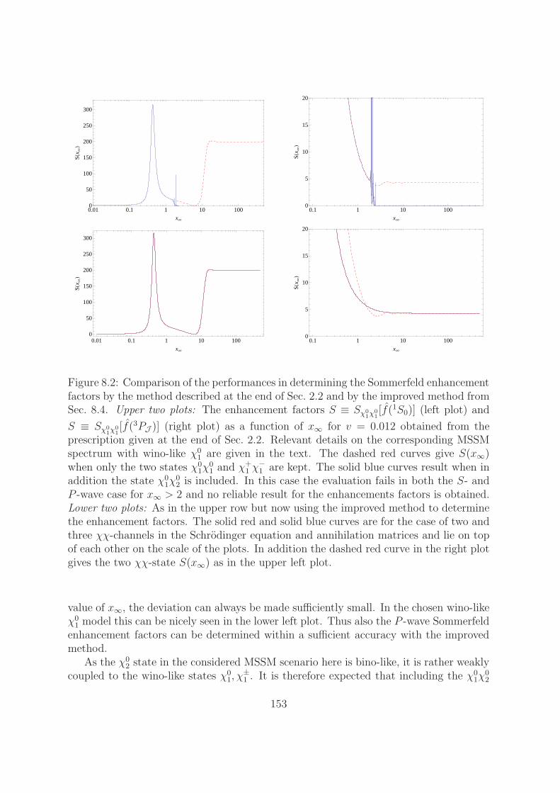
0.01 0.1 1 10 1000
50
100
150
200
250
300
x¥
SHx ¥L
0.1 1 10 1000
5
10
15
20
x¥
SHx ¥L
0.01 0.1 1 10 1000
50
100
150
200
250
300
x¥
SHx ¥L
0.1 1 10 1000
5
10
15
20
x¥
SHx ¥L
Figure 8.2: Comparison of the performances in determining the Sommerfeld enhancementfactors by the method described at the end of Sec. 2.2 and by the improved method fromSec. 8.4. Upper two plots: The enhancement factors S ≡ Sχ0
1χ01[f(1S0)] (left plot) and
S ≡ Sχ01χ
01[f(3PJ )] (right plot) as a function of x∞ for v = 0.012 obtained from the
prescription given at the end of Sec. 2.2. Relevant details on the corresponding MSSMspectrum with wino-like χ0
1 are given in the text. The dashed red curves give S(x∞)when only the two states χ0
1χ01 and χ
+1 χ
−1 are kept. The solid blue curves result when in
addition the state χ01χ
02 is included. In this case the evaluation fails in both the S- and
P -wave case for x∞ > 2 and no reliable result for the enhancements factors is obtained.Lower two plots: As in the upper row but now using the improved method to determinethe enhancement factors. The solid red and solid blue curves are for the case of two andthree χχ-channels in the Schrodinger equation and annihilation matrices and lie on topof each other on the scale of the plots. In addition the dashed red curve in the right plotgives the two χχ-state S(x∞) as in the upper left plot.
value of x∞, the deviation can always be made sufficiently small. In the chosen wino-likeχ01 model this can be nicely seen in the lower left plot. Thus also the P -wave Sommerfeld
enhancement factors can be determined within a sufficient accuracy with the improvedmethod.
As the χ02 state in the considered MSSM scenario here is bino-like, it is rather weakly
coupled to the wino-like states χ01, χ
±1 . It is therefore expected that including the χ0
1χ02
153
state in the Schrodinger equation and annihilation rates has very little effect on the en-hancements of the χ0
1χ01 channel as explicitly confirmed by the calculation in the improved
method.
8.5 Second-derivative operators
In this section we come back to the derivation of the second relation presupposed inSec. 8.1, which is (8.9), and that concerns the connection between the matrix elementsof next-to-next-to-leading order (Pχχ→χχ
e4e3e2e1(2S+1SS)) and corresponding leading-order
(Oχχ→χχe4e3e2e1(
2S+1SS)) S-wave operators. Explicit expressions for the latter operators are
collected in Tab. 5.3 and Tab. 5.2, respectively. In order to confirm (8.9) we show that
〈0|χc†e2Γ(− i
2
←→∂)2χe1|χiχj〉 = κ∗ee′ 〈0|χc†e′2Γχe′1|χiχj〉 . (8.57)
Labels e, e′ are compound indices referring to the two-particle states χe1χe2 and χe′1χe′2,respectively. The definition of κ has been given in (8.11). For completeness we quote ithere again in compound index notation:
κ ee′ = ~p 2e δee′ + 2µeα2
∑
a
mφac(a)ee′ . (8.58)
Making use of (8.18) and (8.26), we can rewrite the left-hand side in (8.57) as
〈0|χc†e2Γ(− i
2
←→∂)2χe1|χiχj〉 = 〈ξ
c†j Γξi〉
∫d3~q
(2π)3~q 2([ψE(~q )]
∗ei + (−1)S [ψE(~q )]∗ei
), (8.59)
where the compound index e refers to the state χe2χe1, while e, as noted before, is used tolabel the corresponding state χe1χe2 . In order to simplify the integral on the right-handside we apply the momentum-space version of the Schrodinger equation (8.28), whichleads to
∫d3~q
(2π)3~q 2 [ψE(~q )]
∗ei = 2µe(2mLSP −Me + E)
∫d3~q
(2π)3[ψE(~q )]
∗ei
− 2µe
∫d3~q
(2π)3d3~k
(2π)3[V ee′(~k )]∗ [ψE(~q − ~k )]∗e′i . (8.60)
The explicit form of the momentum-space potentials, associated with gauge boson andlight Higgs particle exchange, is given by
V ee′(~k ) = 4πα2
∑
a
c(a)ee′
~k2 +m2φa
, (8.61)
where mφa denotes the mass of the exchanged mediator, and the corresponding coeffi-
cients c(a)ee′ are those collected in Tab. B.1. The sum extends over all gauge boson and
154
Higgs mediator particles that can be exchanged in a specific χe1χe2 → χe′1χe′2 potentialscattering reaction.
We can factorise the two integrations in the second line of (8.60) by performing the
shift ~q → ~q + ~k. Using dimensional regularisation, the linearly divergent integral overmomentum ~k can then be evaluated to the finite result
∫dd−1~k
(2π)d−1
1
~k2 +m2φ
d→4= −mφ
4π. (8.62)
Consequently, the right-hand side of (8.59) can be rewritten as
〈0|χc†e2(− i
2
←→∂)2χe1 |χiχj〉 = 〈ξ
c†j Γξi〉
∫d3~q
(2π)3[ψE ]
∗e′i(~q )
×[2µe(2mLSP −Me + E)δe′e + 2µeα2
∑
a
mφac(a) ∗ee′
]+ (−1)S e→ e
= 〈ξc†j Γξi〉∫
d3~q
(2π)3[ψE ]
∗e′i(~q )
(κ∗ee′ + (−1)S κ∗ee′
). (8.63)
In the last equality we have used that the relative momentum associated with the two-particle system χe1χe2, ~pe, is given by ~p 2
e = 2µe(2mLSP−Me+E), such that the term insquare brackets in the second line yields κ∗ee′, see (8.58). Next, let us write the integrandin (8.63) as
[ψE ]∗e′i(~q )
(κ∗ee′ + (−1)S κ∗ee′
)= κ∗ee′ [ψE ]
∗e′i(~q ) + (−1)S κ∗ee′ [ψE ]∗e′i(~q ) , (8.64)
where the index over which summation is carried out in the second term on the right-hand side has been renamed from e to e. Since the potentials for χe1χe2 → χe′1χe′2 and
χe2χe1 → χe′2χe′1 scattering involve the same coupling structure, the relation c(a)ee′ = c
(a)ee′
holds, which implies κee′ = κee′. This allows to eventually obtain
〈0|χc†e2(− i
2
←→∂)2χe1|χiχj〉 = κ∗ee′ 〈ξc†j Γξi〉
∫d3~q
(2π)3
([ψE ]
∗e′i(~q)+ (−1)S [ψE ]∗e′i(~q )
). (8.65)
The summation in the above expression runs over the two-particle states indicated withthe primed labels; while e′ (related to χe1χe2) is varied, the associated label e′ (referringto χe2χe1) changes accordingly. The right-hand side of (8.65) agrees with the right-handside in (8.57), such that the latter relation is proven.
With this relation between the matrix elements of next-to-next-to-leading order andleading-order S-wave operators it is possible to define the effective Wilson coefficients gκ,(8.9, 8.10), that come with the matrix elements of corresponding leading-order S-waveoperators. Let us finally note that the second term in κee′, (8.58), would be absent, ifall exchanged mediator particles would be massless. In the NRMSSM only the potentialfrom photon exchange involves a massless mediator, such that there are typically non-vanishing contributions to the second term related to electroweak gauge boson or Higgsexchange potentials.
155
In Sec. 2.1 we have argued that ladder amplitudes with exchange of massive mediatorsgive only rise to enhanced radiative corrections, if the mediator mass is much smallerthan the masses of the non-relativistic states in the ladder bars. Accordingly, in theNRMSSM only those contributions to the potentials are relevant that arise from gaugeboson or Higgs particle φ exchange with mass mφ ≪ mLSP. As can be seen explicitly
from the momentum space potential expression V (~k ) in (8.61), heavy φb exchange leadsto strongly suppressed contributions to the full potential. Effectively, heavy mediator ex-change thus results in a suppressed local (χ†χ)2 potential interaction. The dominant con-tributions to (8.61) arise from light φa exchange with mφa scaling as the non-relativistic
3-momentum |~k| ∼ mLSPv. This implies that the contributions to κ related to the lightmediators φa are parametrically of the same order, since Me − 2mLSP ∼ E ∼ mLSPv
2
and α2mφa ∼ vmEW ∼ mLSPv2. To the contrary, heavy Higgs boson contributions to
the last term in κ can become large, although the corresponding potential interactionitself is irrelevant. The origin of such unphysical power-counting breaking contributionis the linearly divergent integral (8.62). The simplest solution to eliminate such unphys-ical terms is to decouple heavy Higgs bosons by not including them in the long-rangeNRMSSM potentials discussed in Chap. 7. The decoupling of the corresponding heavystates gives rise to the above mentioned local interaction terms, which count as O(v2)corrections to the NRMSSM long-range potential interactions. As we have neglectedO(v2) corrections to the expressions associated with the long-range effects throughout,we consistently neglect the local potential interactions from heavy mediator exchange.In practical applications, given a specific MSSM spectrum, we eliminate Higgs boson ex-change contributions to the potentials (and thus to κ) if the corresponding Higgs massesfulfil mH > 0.5mLSP, unless mH < 100GeV. Let us remind however, that s-channel ex-change of heavy Higgs states is taken into account in the absorptive parts of the Wilsoncoefficients.
8.6 Approximate treatment of heavy channels
In the preceding sections we have developed a formalism that allows for the calculationof Sommerfeld-corrected co-annihilation rates of non-relativistic, nearly mass-degenerateneutralino and chargino pairs. Consequently, when accounting for Sommerfeld correc-tions on the neutralino and chargino pair-annihilation cross sections in the χ0
1 relic abun-dance calculation, we first have to determine the set of those neutralino and charginopairs χχ for a given MSSM spectrum, which are nearly mass-degenerate with the lightestsuch pair, χ0
1χ01. For these “light” χχ states Sommerfeld-enhanced annihilation rates are
subsequently calculated by means of (8.13) which implies solving corresponding multi-state Schrodinger equations. The latter take the potential and annihilation reactionsamong the non-relativistic and nearly mass-degenerate light χχ pairs with the sameelectric charge and within the same partial wave configuration into account.
Given a specific MSSM spectrum, there will be in general several “heavy” χχ pairsthat do not fulfil the requirement to be nearly mass-degenerate with the χ0
1χ01. These
156

states cannot be part of the NRMSSM neutralino and chargino two-particle pairs. Inprinciple we should thus exclude them a priori, such that they do not appear in theSchrodinger equations and NRMSSM Wilson coefficients. However when keeping thoseheavy χχ states in the EFT ladder diagrams there should be little effect on the en-hancements of the light χχ channels, as the EFT two-particle propagators (8.17) forheavy states (χχ)h with masses Mh ≫ 2mLSP cannot go on-shell and therefore do notcause an enhancement effect. Consequently, it is possible to keep these heavy channelsas internal states in the series of ladder-diagrams, as long as this does not lead in turnto numerical problems in the solution of the corresponding Schrodinger equations. Sincethe improved method described in Sec. 8.4 addresses and solves the issue of numericalinstabilities associated with closed channels in the solution of the Schrodinger equation,there is from the point of view of numerical accuracy no reason why closed heavy chan-nels could not be included in the potentials and annihilation matrices. In particular,there is the possibility that a heavy χχ state has a larger tree-level annihilation ratethan the light two-particle channels, such that the annihilation contributions from theheavy channel can effectively enhance the annihilation rate of a light state. To includesuch effects it is desirable to keep closed heavy channels in the Schrodinger equations.
However, practical limitations on the number of channels that can be treated exactlyin the Schrodinger equations are imposed by CPU time considerations. For example, iffor a given MSSM spectrum and non-relativistic scattering energy E the calculation ofthe factor S[f(1S0)] for the χ
01χ
01 channel within method 2 takes 0.1 s if two channels are
included in the corresponding matrix Schrodinger equation, the CPU time increases to14 s for four included two-particle channels and becomes 5min for 8 channels. Eventually,including all 14 neutral two-particle channels within method-2, the determination of thisspecific S[f(1S0)] takes nearly three hours.9 Even for fixed scattering energy there aretypically several open channels for which Sommerfeld enhancement factors have to becalculated. Moreover, the determination of the thermally averaged annihilation crosssections entering the relic abundance calculation requires an integral over the scatteringenergy. In our application to the χ0
1 relic abundance calculation, CPU considerationstherefore restrict the number of two-particle channels that can be treated exactly in theSchrodinger equations.
In order to cover the case of strong annihilation contributions of closed heavy chan-nels to a light channel’s annihilation rate we allow that heavy channels appear in thelast potential loop before annihilation in the series of ladder-diagrams with incominglight χχ state. However, we neglect heavy channels in all ladder bars apart from the lastloop. This is motivated by non-relativistic power-counting, which shows that there is asuppression factor of the order [E/(Mh − 2mLSP)]
a when a light two-particle channel inthe ladder-diagram is replaced by a heavy channel, where a = 1/2 for the contributionin the last loop before annihilation and a = 3/2 for contributions inside the ladder. Inthe following we describe how the last potential loop contributions of heavy channelscan be absorbed into an effective annihilation matrix. In the determination of the Som-
9The quoted numbers are strongly model and scattering energy E = mLSPv2 dependent. They are
meant as an example to illustrate the effect of the strong increase in CPU time.
157

merfeld enhancement factors we thus solve the Schrodinger equations referring to thesmaller number of light channels only and use in (8.34, 8.35) the yet to define effectiveannihilation matrices that include potential one-loop effects from heavy channels.
Let us start by dividing the N two-particle basis states (χχ)a in a given charge sectorinto n light states treated exactly in the corresponding Schrodinger equations and N −nheavy states that we only include in the last potential loop.10 In the following we usethe compound index h = he1he2 to refer to one of the N − n heavy states. Extending(8.18) to include the contribution from a heavy channel in the last potential loop beforeannihilation, we write
〈0|χc†h2ΓK[− i
2
←→∂]χh1 |χiχj〉 = 〈ξc†j Γξi〉 lim
E→E(−1)
(E − ~p 2
2µij
)
×∫
d3~q
(2π)3
∫d3~k
(2π)3K[~q ] V lh(~q − ~k) 1
E − [Mh − 2mLSP]− ~q 2
2µh
Gil(~p,~k; E)
+ (−1)L+S h→ h , (8.66)
where summation over the compound index l that refers to the light states is implied.Further, Gil denotes the Green function for the Schrodinger operator associated withthe n × n problem of light states. The momentum-space potential V lh encodes thepotential scattering from the light states (χχ)l to the heavy state (χχ)h that undergoesannihilation. Let us now consider the operator matrix elements similar to (8.66), butthis time for all and not only the heavy state operators, multiplied by the correspondingabsorptive parts of Wilson coefficients, f . Making use of (8.26) and taking the heavychannels in the last loop into account as in (8.66), we obtain
fee′ 〈0|χc†e2ΓK[− i
2
←→∂]χe1|χiχj〉 = 2 〈ξc†j Γξi〉
∫d3~q
(2π)3[ψE ]
∗li(~q )
×[fle′K[~q ] + fhe′
∫d3~k
(2π)3K[~k ] V lh(~k − ~q ) 1
E − [Mh − 2mLSP]− ~k 2
2µh
], (8.67)
where the index l runs over the n light and the index h over the N − n heavy channels.The equality in (8.67) holds only if heavy channels contribute exclusively to the lastloop of the ladder-amplitudes prior to annihilation. The form of the right-hand side in(8.67) suggests to rewrite and appropriately simplify the term in square brackets suchthat it eventually describes an effective annihilation matrix f eff
le′K[~q ]. To this end weuse the explicit form of the momentum-space potentials (8.61). The integration over
10Let us recall that we include all neutralino and chargino species in the determination of the relicdensity; however, for the co-annihilation cross sections of heavy neutralino and chargino pairs we usetree-level instead of Sommerfeld-enhanced rates. Contributions of the heavy channels to the thermallyaveraged effective rate 〈σeffv〉 are strongly Boltzmann-suppressed and thus typically negligible, unlessthere is a particular enhancement of the corresponding annihilation rate (such as for example in resonantannihilation), that compensates the Boltzmann suppression.
158
the loop-momentum ~k can then be performed and the expression in square brackets in(8.67) is subsequently written as
f eff, rightll′ = fll′ + Ilh fhl′ , (8.68)
where summation over the compound index h referring to the heavy channels is carriedout. For a better readability we have suppressed the 2S+1LJ wave dependence of theWilson coefficients f = f(2S+1LJ) and f eff = f eff(2S+1LJ) in the last equations. Theexpression Ilh in the second term in (8.68) depends on the orbital angular momentum Lof the corresponding partial wave configuration and is given by
Ilh = α2
∑
a
c(a)lh (−2µh) IL
(2µh(Mh − [2mLSP + E]− iǫ), mφa , ~q
2). (8.69)
A dependence on the total spin enters through the coefficients c(a) of the spin-dependentleading-order potentials. In case of leading-order S-wave matrix elements, where L = 0and K[~q ] = 1, the function IL=0 in (8.69) takes the following form:
I0(y,m, ~q2) =
i
2√~q 2
lni(m2 − y + ~q 2) + 2m
√~q 2
i(m2 − y − ~q 2) + 2√y ~q 2
. (8.70)
In the P -wave case with L = 1 and K[~q ] = ~q we obtain
I1(y,m, ~q2) =
√y −m2~q 2
+i(m2 − y + ~q 2)
2(~q 2)3/2lni(m2 − y + ~q 2) + 2m
√~q 2
i(m2 − y − ~q 2) + 2√y ~q 2
. (8.71)
In (8.68) we have used the superscript label “right” to indicate that with (8.67) we haveconsidered the first half of the corresponding full NRMSSM χiχj forward scatteringmatrix element. Accounting in the same way for the second half, we eventually arrive atthe following effective Wilson coefficients
f effll′ = fll′ + Ilh fhl′ + I∗l′h flh + IlhI
∗l′h′ fhh′ . (8.72)
The expression f effll′ = f eff
ll′ (2S+1LJ ) encodes the hard (off-) diagonal tree-level annihilation
reaction of light χχ states, (χχ)l →∑XAXB → (χχ)l′ , supplemented by potential one-
loop corrections that involve the heavy channels (χχ)h prior to annihilation into theSM and light Higgs particle final states XAXB. The result f eff,right
ll′ in (8.68) is thusassociated with the (χχ)l tree-level annihilation amplitude plus the potential one-loopcorrection arising from heavy channels inside the loop before annihilation. If we takethe index h in (8.68) to run over all (χχ)a pairs in the corresponding charge sector andnot only the heavy channels, then the expression f eff,right
ll′ is related to the leading-ordernon-relativistic approximation to the full one-loop annihilation amplitude for incoming(χχ)l state, which has also been obtained by direct expansion in [93].11
11It can be checked that the loop integrals IS,P defined in [93] are equal to (2π|~q |) I0,1. Let us note that
159

While (8.72) introduces effective Wilson coefficients accounting for potential one-loopcorrections from heavy channels, this expression still involves the factors Ilh and I∗l′h,which in turn imply a dependence on the momentum ~q of the last potential loop beforeannihilation. In the evaluation of (8.67) the knowledge of the full momentum-space wavefunction ψE(~q ) would therefore be needed and not just the corresponding position-spaceexpression and its derivative at the origin. However, we only want to absorb one-loopcorrections of heavy channels (χχ)h with mass-splittings Mh − 2mLSP ≫ E into theeffective Wilson coefficients in (8.72). The typical relative momentum ~q over whichthe last potential-loop integration is carried out scales as ~q 2 ∼ mLSPv
2, such that wecan expand the integrals IL in (8.70, 8.71) in
√~q 2/(Mh − 2mLSPv
2). We keep only theleading-order terms in this expansion, in which case the expressions I0,1 simplify to thefollowing momentum independent terms
I0(y,m, ~q2) → 1√
y +m, I1(y,m, ~q
2) → 2√y +m
3(√y +m)2
. (8.73)
Using these approximations in (8.69) we obtain
Ilh|L=0 = −2µhα2
∑
a
c(a)lh√
yh +mφa
, (8.74)
Ilh|L=1 = −2µhα2
∑
a
c(a)lh
2√yh +mφa
3(√yh +mφa)
2, (8.75)
where yh = 2µh(Mh − [2mLSP + E] − iǫ). Inserting these expressions in the definition(8.72) of the effective Wilson coefficients f eff
ll′ finally provides us with effective Wilsoncoefficients that can be used to obtain local effective annihilation matrices, followingthe prescriptions in Sec. 7.2.1. We will use these effective annihilation matrices in theSommerfeld factors (8.34, 8.35) in order to incorporate effects from heavy channels inthe last potential loop in the annihilation reactions of light incoming (χχ)l pairs.
The adaption of the above steps to the case of second-derivative S-wave operatorsis somewhat more involved, since it requires the application of the equation of motiondiscussed in Sec. 8.5 to the factor K[~k 2] in (8.67). In writing
~k 2 = 2µh
(2mLSP + E −Mh −
[2mLSP + E −Mh −
~k 2
2µh
])(8.76)
in [93] additional terms proportional to the mass differences between the incoming and the virtual χs inthe loop are kept in the non-relativistic expansion, originating from the numerator of the full one-loopamplitude. As we separate in our formalism the long-distance from the short-range physics, the lattermass difference terms can contribute to O(v2) corrections to the long-distance part – which we neglect– or to O(v2) corrections to the short-distance annihilations. We have kept the latter contributions bytaking all mass-difference terms δm, δm in the Wilson coefficients into account, see Chaps. 5 and 6. Itis worth to add that there are further sources of terms proportional to mass differences that have beenneglected in [93] and in our approach. For instance, there is the anti-particle pole contribution in theq0-integration of the full amplitude which we neglect as it belongs to a class of O(v2) corrections to thelong-range interactions. In [93] these corrections from the anti-particle pole have been omitted as well.
160

and noting the corresponding steps in Sec. 8.5 we finally obtain the following result forthe effective Wilson coefficients associated with second-derivative operators:
geffκ,ll′ = gκ,ll′
+1
2
[Ilh,D2
ghl′
M2+ I∗l′h,D2
glhM2
+ Ilh|L=0I∗l′h′,D2
ghh′
M2+ Ilh,D2I∗l′h′|L=0
ghh′
M2
]. (8.77)
The expression Ilh,D2 introduced above reads
Ilh,D2 = 2µhα2
((2mLSP + E −Mh)(−2µh)
∑
a
c(a)lh√
yh +mφa
+∑
a
mφa c(a)lh
). (8.78)
Note that a dependence on the spin S = 0, 1 is implicit through the coefficients c(a)
associated with the spin-dependent leading-order potentials (8.61). Further let us notethat the mass scale M in each term in (8.77) is defined by the masses of the two χχpairs specified by the indices of the accompanying Wilson coefficients g. For the genericdefinition of this process-specific mass scale see (5.12).
This concludes the presentation of our EFT set-up, which allows to determine Som-merfeld-enhanced co-annihilation rates of a set of nearly mass-degenerate “light” χχpairs including effects from heavy channels in the last potential loop before annihilation.In Chap. 9 we apply this formalism to the calculation of the χ0
1 relic abundance includingSommerfeld enhancements, providing a detailed study for several MSSM benchmark sce-narios. In that chapter we will also address the question how the neutralino and charginotwo-particle states should be divided into light and heavy channels. If not noted oth-erwise, the potential one-loop corrections from heavy channels will be included in theanalysis by using corresponding effective annihilation matrices obtained from (8.72) and(8.77) in the formula for the Sommerfeld enhancement factors. At the end of Chap. 9 wewill additionally discuss the comparison of the relic abundance results when heavy chan-nels are treated approximately in the last potential loop of corresponding co-annihilationrates with the respective result, where those heavy channels are taken into account ex-actly in the Schrodinger equations. In anticipation of results from Sec. 9.5 let us notethat the perturbative treatment of effects from heavy states for the MSSM scenariostudied therein gives a very good approximation to the results where the heavy statesare considered exactly in the Schrodinger equations. From this we conclude that theapproximate treatment of heavy states is often a good approximation to the result fromfull resummation. However, this does not imply that either of the two, the approximateor exact treatment, is a good approximation to the true one-loop corrections from heavychannels. Generically we cannot expect that we obtain a good approximation to the fullone-loop results with heavy internal states, if we use the non-relativistic approximationin the potential region for the latter, because the non-relativistic expansion breaks downfor large mass splitting terms [Mh−2mLSP]. Nevertheless, as noted before, heavy channelloops are at least suppressed by (E/[Mh − 2mLSP])
1/2 with respect to the light channelcontributions. As the impact of heavy states on the Sommerfeld enhancements of light
161

(χχ)l channels is in any case rather small, we decide to include their effect by using theeffective Wilson coefficients (8.72, 8.77).
162
Chapter 9
Benchmark models in the generalMSSM
In the preceding chapters we have developed a non-relativistic MSSM effective theoryframework, the NRMSSM, that allows to systematically address the calculation of en-hanced radiative corrections in pair-annihilation rates of non-relativistic and nearly mass-degenerate neutralino and chargino states in the general MSSM. The focus has been onthe construction of the effective theory and on a detailed description of the relevanttechnical aspects in the NRMSSM calculation of Sommerfeld-enhanced rates. Here weapply the framework to several well-motivated MSSM scenarios with heavy neutralinoLSP and investigate in particular the impact of Sommerfeld enhancements on the χ0
1
relic abundance calculation. The underlying physics effects are analysed in detail ineach step of the calculation, which allows to illustrate the general use of our effectivetheory set-up applicable in the general MSSM. Furthermore, the question of viability ofpopular MSSM scenarios in light of a consistent treatment of the Sommerfeld effect canbe addressed.
We choose to consider three scenarios taken from the set of Snowmass pMSSM bench-mark models [98]. These models pass all constraints from so far unsuccessful SUSYsearches at the LHC, additional collider, flavour and precision measurement bounds aswell as constraints from dark matter direct detection experiments and indirect searches.The neutralino LSP relic abundance within these models, calculated from perturbativeannihilation rates, is not larger than the WMAP bound, but can be smaller than the ex-perimentally measured value. The latter allows for the case that neutralino dark matterdoes not make up all the cosmic cold dark matter. In addition to these benchmark scenar-ios we investigate the Sommerfeld enhancements in neutralino/chargino co-annihilationsin a set of models interpolating between a scenario with almost pure-higgsino χ0
1 toa wino-like χ0
1 model. The MSSM spectra for the models on this “higgsino-to-wino”trajectory are generated with DarkSUSY [5]. As our work allows for the first time aconsistent study of the Sommerfeld effect on the relic abundance calculation for mod-els with mixed wino-higgsino neutralino LSP we provide an extensive discussion of theSommerfeld effect in such a scenario.
163
We start our analysis in Sec. 9.1 with the investigation of a wino-like χ01 benchmark
model taken from the set of Snowmass pMSSM benchmark scenarios in [98]. Sec. 9.2contains the analysis of a corresponding higgsino-like χ0
1 Snowmass model. In both caseswe compare to results obtained in the well-studied “pure” wino and higgsino scenarioswhere the χ0
1 is assumed to be part of an unbroken SU(2)L triplet or two unbrokenSU(2)L doublets. As Sommerfeld enhancements have been studied extensively in theparticular case of a pure wino χ0
1 in the literature, we address the question of the validityof conclusions inferred from these pure wino and higgsino scenarios to wino- and higgsino-like χ0
1 spectra in the general MSSM. In Sec. 9.3 the effect of Sommerfeld enhancementsin co-annihilations of wino-like neutralino and chargino states in a bino-like χ0
1 pMSSMbenchmark scenario is considered. A “higgsino-to-wino” trajectory is defined in Sec. 9.4,by introducing 13 models that interpolate between a higgsino- and wino-like χ0
1 spectrumwhile the relic density calculated from perturbative rates is kept fixed. Our discussionhere is focused on the spectra and the obtained relic abundances omitting particulardetails on the Sommerfeld enhanced co-annihilation cross sections. The specific featuresof the Sommerfeld effect for a mixed wino-higgsino χ0
1 are subsequently studied in detailin Sec. 9.5, where the selected spectrum is one of the trajectory models of the precedingsection.
9.1 Wino-like χ01
Wino-like χ01 dark matter arranges into an approximate SU(2)L fermion triplet together
with the two chargino states χ±1 . In the SU(2)L × U(1)Y symmetric limit the triplet
would be assigned zero hypercharge. All states χ01, χ
±1 share the same O(TeV) mass
scale, characterised by the wino mass parameter M2, mχ ∼ |M2|. As discussed inSec. 4.3, electroweak symmetry-breaking introduces a small mass splitting between theneutral and the charged components of the triplet; the tree-level mass splitting happensto be very small, O(m4
W/m3SUSY), and the one-loop radiative corrections dominate over
the tree-level splitting.
A pMSSM scenario with wino-like χ01 is provided by the SUSY spectrum with model
ID 2392587 in [98]. A measure for the wino fraction of a given neutralino LSP state is thesquare of the modulus of the neutralino mixing-matrix entry ZN 21. For the SnowmasspMSSM scenario 2392587 the χ0
1 constitutes a rather pure wino, |ZN 21|2 = 0.999, witha mass mLSP ≡ mχ0
1= 1650.664GeV. The mass of the chargino partner χ±
1 is given bymχ+
1= 1650.819GeV, such that δm = mχ+
1−mχ0
1turns out to be 0.155GeV. Without
any modification these values are taken from the spectrum card provided by [98] wherethe mass parameters refer to the DR-scheme. As the precise sub O(GeV)-scale χ0
1χ±1
mass splitting is an essential ingredient in the calculation of the Sommerfeld-enhancedco-annihilation rates we have to assume an accuracy of the given mass spectrum at thelevel of 10MeV for our analysis of the Sommerfeld enhancement in the pMSSM scenarioto be meaningful. A rigorous analysis of Sommerfeld-enhanced co-annihilation processesin a given model should refer to the on-shell mass spectrum of the neutralino and chargino
164
states instead of DR-parameters, where a sub-GeV scale precision of the mass parametersrequires the consideration of one-loop renormalised quantities. For reference purposes,however, we do not modify the publicly available DR-spectra of [98] for all three pMSSMmodels discussed here.
In the context of minimal dark matter models [28], wino dark matter is realised as theneutral component of an approximate SU(2)L triplet state as well. In contrast to MSSMscenarios with wino-like χ0
1, the SU(2)L triplet minimal dark matter models (referredto as “pure-wino” models in the following) consider interactions of the dark matterstates with the electroweak gauge bosons only. Two-particle final states in minimaldark matter pair-annihilation reactions are hence given by pairs of SM particles andthe SM Higgs boson and all heavier states above the minimal dark matter mass scaleare treated as completely decoupled. Such a scenario agrees with the decoupling limitin a MSSM scenario with wino-like χ0
1 LSP. To the contrary, the wino-like pMSSMmodel that we consider here features non-decoupled sfermion states at the 2 − 3TeVscale with non-vanishing couplings of the χ0
1 and χ±1 to sfermions and to the (heavier)
Higgs states, though the latter are suppressed with respect to the couplings to the gaugebosons, because any Higgs-χχ (tree-level) interaction takes place between the gaugino-component of the one and the higgsino-component of the other χ. As the higgsino-likeneutralino and chargino states in the pMSSM model under consideration reside at theO(3.9TeV) scale any Higgs-χχ interaction plays a sub-dominant role in our analysis ofpair-annihilation reactions of the wino-like χ0
1 and χ±1 states. Due to the non-decoupled
sfermion states though, some annihilation rates in the wino-like χ01 pMSSM scenario are
reduced with respect to the pure-wino dark matter case.
In the calculation of the relic abundance we have to take into account all possibletwo-particle co-annihilation reactions between the (approximate) SU(2)L triplet statesχ01, χ
±1 . In addition, in the pMSSM model 2392587, the bino-like χ0
2 is only about 8%heavier than the χ0
1, mχ02= 1781.37GeV. Hence the χ0
2 is a potentially relevant co-annihilating particle as well. It turns out though, that this state eventually plays no rolefor the relic abundance, as the corresponding cross sections are strongly suppressed withrespect to those of the wino-like particles χ0
1 and χ±1 due to the much weaker couplings
of the bino-like χ0 to gauge bosons and to the remaining χ0/χ± states. All remainingheavier particles in the pMSSM scenario lie above the 2TeV scale, so they are alreadyBoltzmann suppressed and hence practically irrelevant during the χ0
1 freeze-out.
Sommerfeld enhancements on the co-annihilation rates are taken into account by in-cluding in the multi-state Schrodinger equations, discussed in context of the NRMSSMin Chap. 8, all χχ two-particle states with mass smaller than Mmax = 2mχ0
1+mχ0
1v2max,
where we set vmax = 1/3. This choice is motivated by the fact that vmax roughly cor-responds to the χ0
1’s mean velocity around freeze-out, hence these states are potentiallyrelevant for co-annihilation processes, and can still be produced on-shell in a χ0
1χ01 scat-
tering process. The remaining heavier two-particle states with mass above Mmax areincluded in the computation of the Sommerfeld enhancement of the lighter states inthe last loop before the annihilation, following the method developed in Sec. 8.6. Theχχ-channels, whose long-distance interactions are treated exactly, can be classified ac-
165

cording to their total electric charge. The sector of neutral two-particle states comprisesthe χ0
1χ01 and χ+
1 χ−1 channels. In the pMSSM scenario considered here, this sector con-
tains in addition the χ01χ
02 state. In the single-charged and the double-charged sectors
of a pure-wino dark matter scenario there is only one state present in each sector, χ01χ
+1
(χ01χ
−1 ) and χ
+1 χ
+1 (χ−
1 χ−1 ), whereas in the pMSSM scenario we have to add in addition
a second state with χ01 replaced by χ0
2, in agreement with the rule above that defines thechannels which enter the Schrodinger equation. Since the bino-like neutralino essentiallyneither couples to the wino-like particles nor to gauge bosons, and because sfermionstates are rather heavy, potential interactions as well as tree-level annihilation reactionsinvolving the bino-like χ0
2 are strongly suppressed with respect to the corresponding in-teractions with wino-like particles χ0
1, χ±1 . As a consequence, χ0
2 plays essentially no rolefor Sommerfeld enhancements, and we focus the discussion that follows on the channelsbuilt from the wino-like χ0
1 and χ±1 states only.
In each of the charge sectors long-range interactions due to potential exchange ofelectroweak gauge bosons, photons and light Higgses are present.1 Potential W -bosonexchange leads to a Yukawa potential interaction that induces transitions between theχ01χ
01 and the χ+
1 χ−1 state in the neutral sector. Hence the part of the neutral sector
consisting of the channels χ01χ
01 and χ+
1 χ−1 is characterised by a potential matrix with
non-vanishing off-diagonals which are of the same strength as the diagonal entries. Asthe incoming χ0
1χ01 pair cannot build a 3S1 or 1P1 state, potential interactions are re-
sponsible for transitions between the two neutral states χ01χ
01 and χ+
1 χ−1 in a 1S0 or 3PJ
configuration.In Fig. 9.1 we plot the enhancement (σSFv)/(σpertv) of annihilation rates including
long-range interactions, σSFv ≡ σSFvrel, with respect to the perturbative tree-level result,σpertv ≡ σpertvrel, for the two-particle states χ0
1χ01 and χ+
1 χ−1 in the neutral sector of the
model as a function of the velocity vLSP of the incoming χ01’s in their centre-of-mass
frame. We define the velocity vLSP by√s = 2mχ0
1+ mχ0
1v2LSP with
√s the available
centre-of-mass energy. The spin-averaged inclusive tree-level annihilation rates σpertvare calculated in the non-relativistic approximation
σpertv = a + b v2 + O(v4) , (9.1)
and are obtained from the appropriate sum over the exclusive rates in (6.24) includingO(v2rel) effects. In case of the χ0
1χ01 state the relation between the relative velocity v and
vLSP is given by v = 2 vLSP. For χ+1 χ
−1 annihilation reactions the relation is
v = 2Re√mχ0
1/mχ+
1[v2LSP − 2 δm/mχ0
1] . (9.2)
The coefficients a and b in (9.1) are determined from the absorptive part of partial-wavedecomposed Wilson coefficients as discussed in Chap. 6. In case of the Sommerfeld-
1Potentials from Higgs exchange are negligible compared to the leading contributions from gaugebosons in the pMSSM scenario with wino-like χ0
1, again because in any Higgs-χχ vertex the gauginocomponent of one χ is coupled to the higgsino component of the other χ. In the wino-like χ0
1 Snowmassmodel the lowest-lying χ’s relevant for the Sommerfeld effect are rather pure wino-like χ0 and χ± stateswith a very small higgsino component.
166
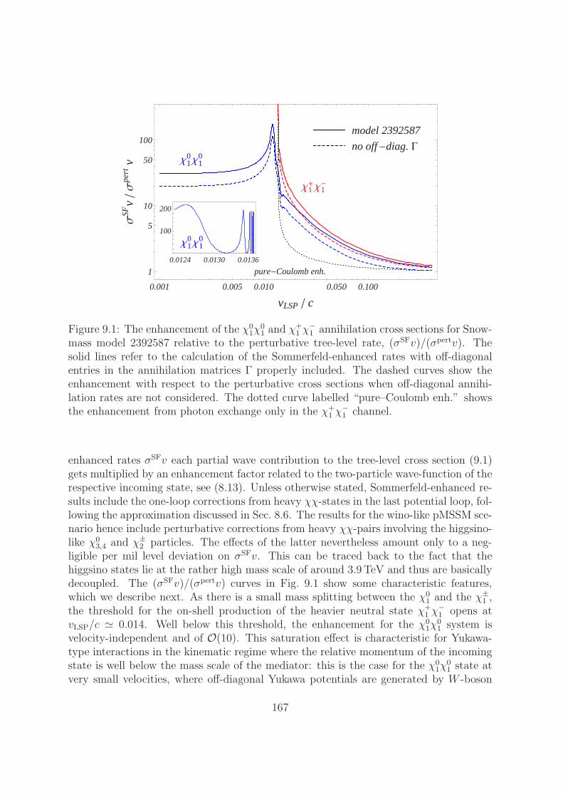
Χ1+Χ1-
Χ10Χ1
0
0.001 0.005 0.010 0.050 0.100
1
5
10
50
100
vLSP c
ΣSF
vΣ
pert
vmodel 2392587
no off-diag. G
pure-Coulomb enh.
Χ10Χ1
0
0.0124 0.0130 0.0136
100
200
Figure 9.1: The enhancement of the χ01χ
01 and χ
+1 χ
−1 annihilation cross sections for Snow-
mass model 2392587 relative to the perturbative tree-level rate, (σSFv)/(σpertv). Thesolid lines refer to the calculation of the Sommerfeld-enhanced rates with off-diagonalentries in the annihilation matrices Γ properly included. The dashed curves show theenhancement with respect to the perturbative cross sections when off-diagonal annihi-lation rates are not considered. The dotted curve labelled “pure–Coulomb enh.” showsthe enhancement from photon exchange only in the χ+
1 χ−1 channel.
enhanced rates σSFv each partial wave contribution to the tree-level cross section (9.1)gets multiplied by an enhancement factor related to the two-particle wave-function of therespective incoming state, see (8.13). Unless otherwise stated, Sommerfeld-enhanced re-sults include the one-loop corrections from heavy χχ-states in the last potential loop, fol-lowing the approximation discussed in Sec. 8.6. The results for the wino-like pMSSM sce-nario hence include perturbative corrections from heavy χχ-pairs involving the higgsino-like χ0
3,4 and χ±2 particles. The effects of the latter nevertheless amount only to a neg-
ligible per mil level deviation on σSFv. This can be traced back to the fact that thehiggsino states lie at the rather high mass scale of around 3.9TeV and thus are basicallydecoupled. The (σSFv)/(σpertv) curves in Fig. 9.1 show some characteristic features,which we describe next. As there is a small mass splitting between the χ0
1 and the χ±1 ,
the threshold for the on-shell production of the heavier neutral state χ+1 χ
−1 opens at
vLSP/c ≃ 0.014. Well below this threshold, the enhancement for the χ01χ
01 system is
velocity-independent and of O(10). This saturation effect is characteristic for Yukawa-type interactions in the kinematic regime where the relative momentum of the incomingstate is well below the mass scale of the mediator: this is the case for the χ0
1χ01 state at
very small velocities, where off-diagonal Yukawa potentials are generated by W -boson
167
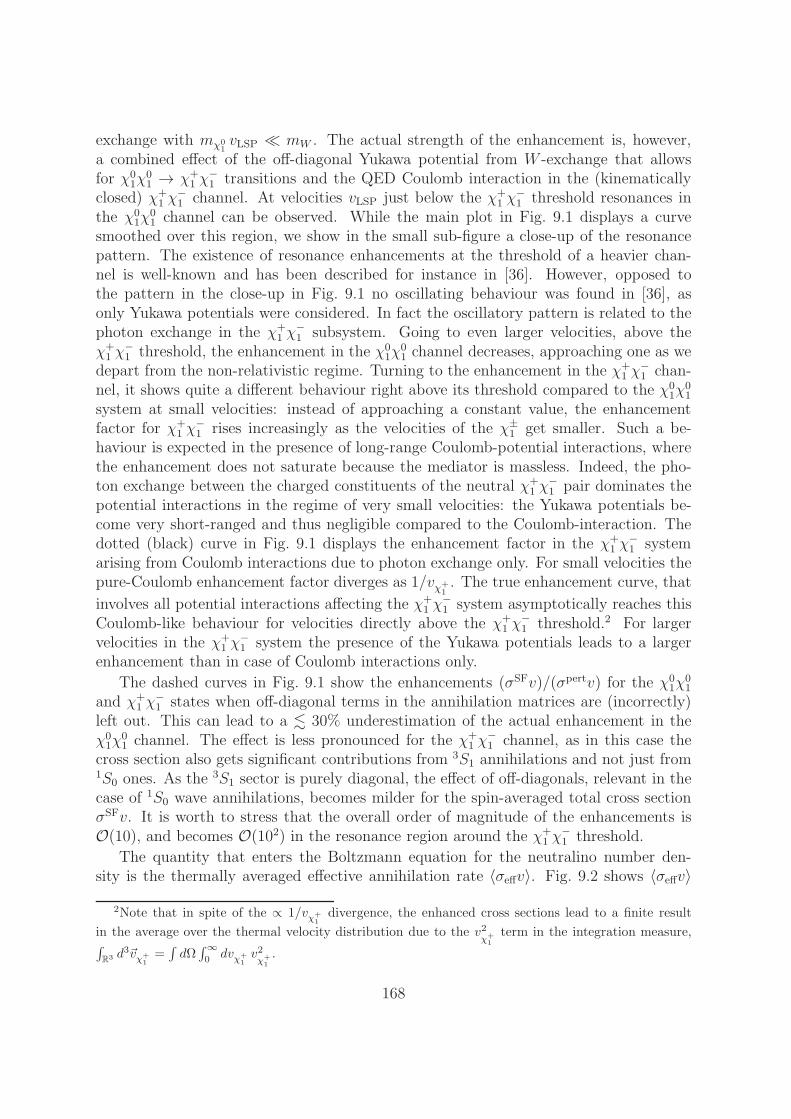
exchange with mχ01vLSP ≪ mW . The actual strength of the enhancement is, however,
a combined effect of the off-diagonal Yukawa potential from W -exchange that allowsfor χ0
1χ01 → χ+
1 χ−1 transitions and the QED Coulomb interaction in the (kinematically
closed) χ+1 χ
−1 channel. At velocities vLSP just below the χ+
1 χ−1 threshold resonances in
the χ01χ
01 channel can be observed. While the main plot in Fig. 9.1 displays a curve
smoothed over this region, we show in the small sub-figure a close-up of the resonancepattern. The existence of resonance enhancements at the threshold of a heavier chan-nel is well-known and has been described for instance in [36]. However, opposed tothe pattern in the close-up in Fig. 9.1 no oscillating behaviour was found in [36], asonly Yukawa potentials were considered. In fact the oscillatory pattern is related to thephoton exchange in the χ+
1 χ−1 subsystem. Going to even larger velocities, above the
χ+1 χ
−1 threshold, the enhancement in the χ0
1χ01 channel decreases, approaching one as we
depart from the non-relativistic regime. Turning to the enhancement in the χ+1 χ
−1 chan-
nel, it shows quite a different behaviour right above its threshold compared to the χ01χ
01
system at small velocities: instead of approaching a constant value, the enhancementfactor for χ+
1 χ−1 rises increasingly as the velocities of the χ±
1 get smaller. Such a be-haviour is expected in the presence of long-range Coulomb-potential interactions, wherethe enhancement does not saturate because the mediator is massless. Indeed, the pho-ton exchange between the charged constituents of the neutral χ+
1 χ−1 pair dominates the
potential interactions in the regime of very small velocities: the Yukawa potentials be-come very short-ranged and thus negligible compared to the Coulomb-interaction. Thedotted (black) curve in Fig. 9.1 displays the enhancement factor in the χ+
1 χ−1 system
arising from Coulomb interactions due to photon exchange only. For small velocities thepure-Coulomb enhancement factor diverges as 1/vχ+
1. The true enhancement curve, that
involves all potential interactions affecting the χ+1 χ
−1 system asymptotically reaches this
Coulomb-like behaviour for velocities directly above the χ+1 χ
−1 threshold.2 For larger
velocities in the χ+1 χ
−1 system the presence of the Yukawa potentials leads to a larger
enhancement than in case of Coulomb interactions only.
The dashed curves in Fig. 9.1 show the enhancements (σSFv)/(σpertv) for the χ01χ
01
and χ+1 χ
−1 states when off-diagonal terms in the annihilation matrices are (incorrectly)
left out. This can lead to a . 30% underestimation of the actual enhancement in theχ01χ
01 channel. The effect is less pronounced for the χ+
1 χ−1 channel, as in this case the
cross section also gets significant contributions from 3S1 annihilations and not just from1S0 ones. As the 3S1 sector is purely diagonal, the effect of off-diagonals, relevant in thecase of 1S0 wave annihilations, becomes milder for the spin-averaged total cross sectionσSFv. It is worth to stress that the overall order of magnitude of the enhancements isO(10), and becomes O(102) in the resonance region around the χ+
1 χ−1 threshold.
The quantity that enters the Boltzmann equation for the neutralino number den-sity is the thermally averaged effective annihilation rate 〈σeffv〉. Fig. 9.2 shows 〈σeffv〉
2Note that in spite of the ∝ 1/vχ+
1
divergence, the enhanced cross sections lead to a finite result
in the average over the thermal velocity distribution due to the v2χ+
1
term in the integration measure,∫R3 d
3~vχ+
1
=∫dΩ∫∞
0 dvχ+
1
v2χ+
1
.
168
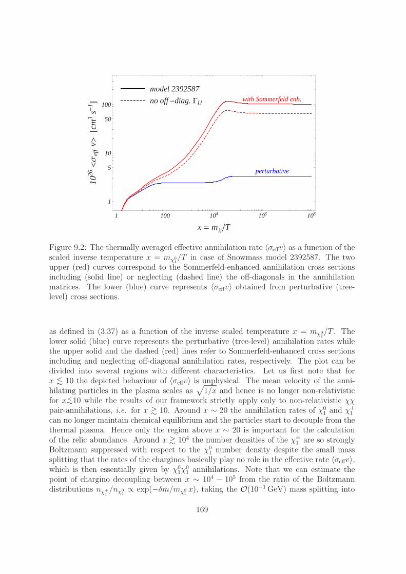
1 100 104 106 108
1
5
10
50
100
x = mΧT
1026<Σ
eff
v>@c
m3
s-1 D
model 2392587
no off-diag. GIJwith Sommerfeld enh.
perturbative
Figure 9.2: The thermally averaged effective annihilation rate 〈σeffv〉 as a function of thescaled inverse temperature x = mχ0
1/T in case of Snowmass model 2392587. The two
upper (red) curves correspond to the Sommerfeld-enhanced annihilation cross sectionsincluding (solid line) or neglecting (dashed line) the off-diagonals in the annihilationmatrices. The lower (blue) curve represents 〈σeffv〉 obtained from perturbative (tree-level) cross sections.
as defined in (3.37) as a function of the inverse scaled temperature x = mχ01/T . The
lower solid (blue) curve represents the perturbative (tree-level) annihilation rates whilethe upper solid and the dashed (red) lines refer to Sommerfeld-enhanced cross sectionsincluding and neglecting off-diagonal annihilation rates, respectively. The plot can bedivided into several regions with different characteristics. Let us first note that forx . 10 the depicted behaviour of 〈σeffv〉 is unphysical. The mean velocity of the anni-hilating particles in the plasma scales as
√1/x and hence is no longer non-relativistic
for x<∼10 while the results of our framework strictly apply only to non-relativistic χχpair-annihilations, i.e. for x & 10. Around x ∼ 20 the annihilation rates of χ0
1 and χ+1
can no longer maintain chemical equilibrium and the particles start to decouple from thethermal plasma. Hence only the region above x ∼ 20 is important for the calculationof the relic abundance. Around x & 104 the number densities of the χ±
1 are so stronglyBoltzmann suppressed with respect to the χ0
1 number density despite the small masssplitting that the rates of the charginos basically play no role in the effective rate 〈σeffv〉,which is then essentially given by χ0
1χ01 annihilations. Note that we can estimate the
point of chargino decoupling between x ∼ 104 − 105 from the ratio of the Boltzmanndistributions nχ+
1/nχ0
1∝ exp(−δm/mχ0
1x), taking the O(10−1GeV) mass splitting into
169
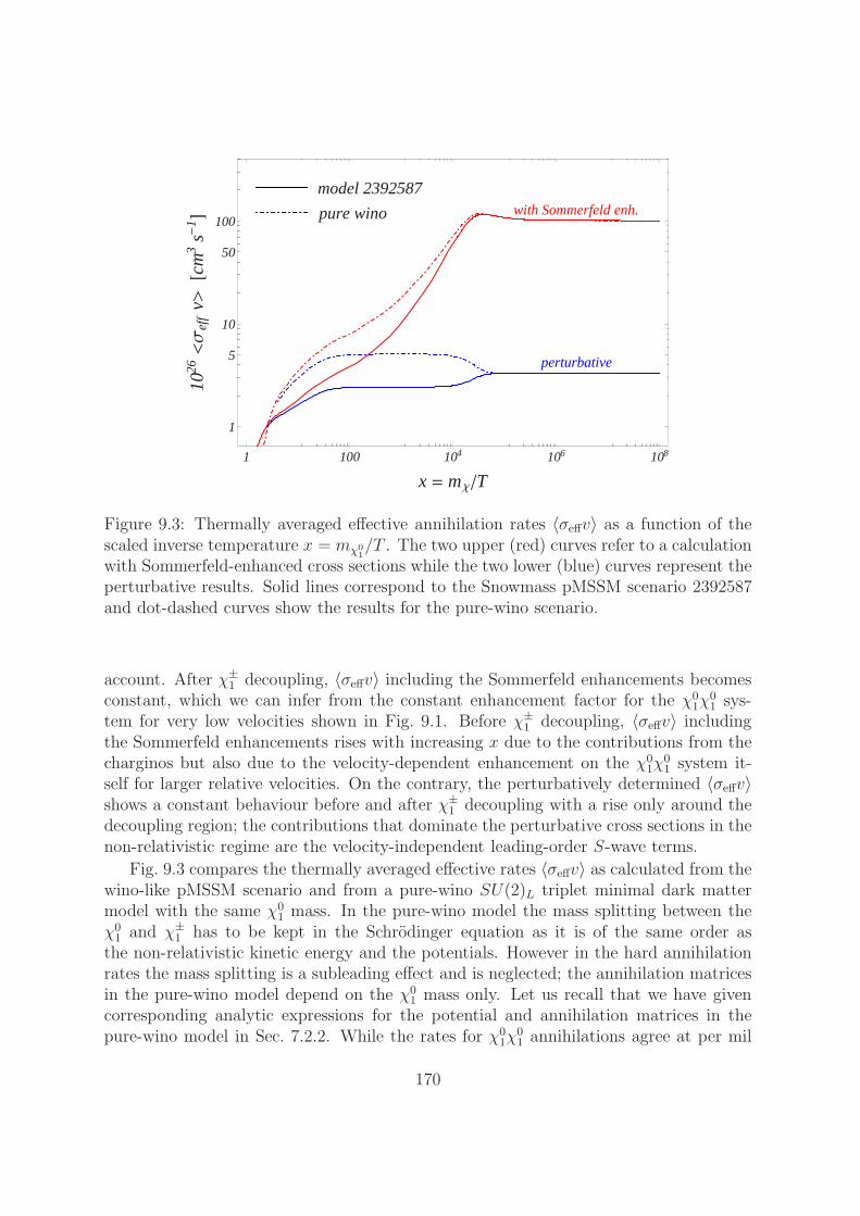
1 100 104 106 108
1
5
10
50
100
x = mΧT
1026<Σ
eff
v>@c
m3
s-1 D
model 2392587
pure wino with Sommerfeld enh.
perturbative
Figure 9.3: Thermally averaged effective annihilation rates 〈σeffv〉 as a function of thescaled inverse temperature x = mχ0
1/T . The two upper (red) curves refer to a calculation
with Sommerfeld-enhanced cross sections while the two lower (blue) curves represent theperturbative results. Solid lines correspond to the Snowmass pMSSM scenario 2392587and dot-dashed curves show the results for the pure-wino scenario.
account. After χ±1 decoupling, 〈σeffv〉 including the Sommerfeld enhancements becomes
constant, which we can infer from the constant enhancement factor for the χ01χ
01 sys-
tem for very low velocities shown in Fig. 9.1. Before χ±1 decoupling, 〈σeffv〉 including
the Sommerfeld enhancements rises with increasing x due to the contributions from thecharginos but also due to the velocity-dependent enhancement on the χ0
1χ01 system it-
self for larger relative velocities. On the contrary, the perturbatively determined 〈σeffv〉shows a constant behaviour before and after χ±
1 decoupling with a rise only around thedecoupling region; the contributions that dominate the perturbative cross sections in thenon-relativistic regime are the velocity-independent leading-order S-wave terms.
Fig. 9.3 compares the thermally averaged effective rates 〈σeffv〉 as calculated from thewino-like pMSSM scenario and from a pure-wino SU(2)L triplet minimal dark mattermodel with the same χ0
1 mass. In the pure-wino model the mass splitting between theχ01 and χ±
1 has to be kept in the Schrodinger equation as it is of the same order asthe non-relativistic kinetic energy and the potentials. However in the hard annihilationrates the mass splitting is a subleading effect and is neglected; the annihilation matricesin the pure-wino model depend on the χ0
1 mass only. Let us recall that we have givencorresponding analytic expressions for the potential and annihilation matrices in thepure-wino model in Sec. 7.2.2. While the rates for χ0
1χ01 annihilations agree at per mil
170

1 100 104 106 108
0.6
0.7
0.8
0.9
1.0
x = mΧ T
Y
Ype
rtmodel 2392587
no off-diag. G
pure wino
Figure 9.4: The ratios of the yield Y/Ypert as a function of x = mχ01/T , where Y is
calculated including the Sommerfeld enhancement on the χχ annihilation rates whileYpert just uses the perturbative ones. The solid (blue) and dashed (black) curves givethe results for the Snowmass model 2392587 including and neglecting off-diagonal anni-hilation rates, respectively. The dot-dashed (red) curve corresponds to Y/Ypert(x) in thepure-wino model.
level, the cross sections involving χ±1 are generically larger by factors of O(1) in the pure-
wino model as compared to the pMSSM wino-like model. This can be mainly traced backto the destructive interference between t-channel sfermion and s-channel Z (and Higgs-boson) exchange amplitudes in χ+
1 χ−1 → ff annihilations in the pMSSM scenario case,
while the t-channel sfermion exchange amplitudes are absent in the pure-wino model.In addition the pure-wino case neglects all final state masses which in particular givesrise to larger annihilation rates into the tt and electroweak gauge boson final states ascompared to the pMSSM scenario, where the non-vanishing masses of all SM particlesare taken into account. This accounts for the deviation between the curves in Fig. 9.3before χ±
1 decoupling.Finally we consider the yield Y = n/s, defined in (3.22) as the ratio of the number
density n of all co-annihilating particle species divided by the entropy density s in thecosmic co-moving frame. As discussed in Chap. 3, the dependence of the yield on thescaled inverse temperature x = mχ0
1/T is governed by the Boltzmann equation (3.28),
and the χ01 relic abundance is obtained from the yield today, see (3.31). In Fig. 9.4 we
show the ratio of the yield Y calculated from Sommerfeld-enhanced cross sections in boththe pMSSM and the pure-wino model to the corresponding results using perturbative
171
cross sections, Ypert, as a function of x.
First note, that the denominator Ypert in the ratio Y/Ypert differs for the pMSSM andthe pure-wino model, which is a consequence of the different effective rates 〈σeffv〉, seeFig. 9.3. Further, in case of the pMSSM scenario we show results corresponding to acalculation of Y including and neglecting off-diagonal annihilation rates. Around x ∼ 20the yields including Sommerfeld enhancements start to depart from the correspondingperturbative results; the enhanced rates delay the freeze-out of interactions, which leadsto a reduction of the yield Y compared to the perturbative result Ypert. The most drasticreduction in Y/Ypert occurs between x ∼ 20 and x ∼ 103. In this region the enhancementfactors on the cross sections are of O(10) (and not yet O(102) as for very large x), leadingto Y/Ypert values that deviate from 1 by a few 10%. For x & 105 the fraction Y/Ypertstays constant, meaning that at these temperatures the particle abundances in both theperturbative and Sommerfeld-enhanced calculation are frozen in. In case of the wino-likemodel we find that the relic densities calculated from the yield today read Ωperth2 = 0.112and ΩSFh2 = 0.066. Hence taking into account the Sommerfeld effect leads to a reductionof the calculated relic abundance of around 40%. On the other hand, neglecting the off-diagonal annihilations in the calculation of Sommerfeld-enhanced rates overestimates therelic density by 15% compared to the correct ΩSFh2. Let us recall that the relic densitycalculated without corrections from heavy χχ-states in the last potential loop differsfrom the ΩSFh2 value quoted above at most at the per mil level. Due to overall largerhard annihilation rates in the pure-wino model, the calculated relic density includingSommerfeld-enhanced rates turns out to be ΩSF
pure-wh2 = 0.034, while the corresponding
perturbative result is Ωpertpure-wh
2 = 0.056.
A quantification of the theoretical error on such numbers is difficult. In conventionaltree-level calculations of annihilation cross sections and the ensuing determination of relicdensities neglecting radiative corrections, the results on the relic densities are supposedto be accurate to O(5%) in the absence of enhanced corrections due to non-relativisticscattering, large Sudakov logarithms, or, potential strong-interaction effects for quarkand gluon final states. The latter two restrictions still apply when the Sommerfeld effectis included. Further, our computation of the Sommerfeld effect itself neglects O(v2)corrections to the scattering potentials as well as ordinary, non-enhanced correctionsto the short-distance annihilation coefficients. Hence the accuracy of the Sommerfeld-corrected annihilation cross sections and relic densities is presumably again at the O(5%)accuracy level at best.
9.2 Higgsino-like χ01
The higgsino-like neutralino χ01 arises as the lightest out of four mass eigenstates χ0
1,2, χ±1
related to two SU(2)L fermion doublets. Note that the hypercharges of the two SU(2)Ldoublets are given by Y = ±1/2 respectively, which ensures the electric neutrality of theχ01. The common mass scale of the χ0
1,2, χ±1 states is set by the O(TeV) higgsino mass
parameter, mχ ∼ |µ|. Electroweak symmetry breaking introduces a tree-level splitting
172
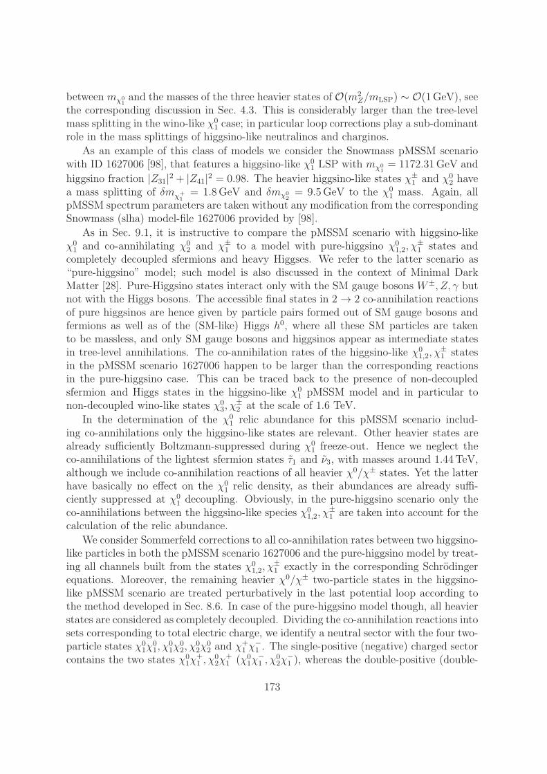
between mχ01and the masses of the three heavier states of O(m2
Z/mLSP) ∼ O(1GeV), seethe corresponding discussion in Sec. 4.3. This is considerably larger than the tree-levelmass splitting in the wino-like χ0
1 case; in particular loop corrections play a sub-dominantrole in the mass splittings of higgsino-like neutralinos and charginos.
As an example of this class of models we consider the Snowmass pMSSM scenariowith ID 1627006 [98], that features a higgsino-like χ0
1 LSP with mχ01= 1172.31GeV and
higgsino fraction |Z31|2 + |Z41|2 = 0.98. The heavier higgsino-like states χ±1 and χ0
2 havea mass splitting of δmχ+
1= 1.8GeV and δmχ0
2= 9.5GeV to the χ0
1 mass. Again, allpMSSM spectrum parameters are taken without any modification from the correspondingSnowmass (slha) model-file 1627006 provided by [98].
As in Sec. 9.1, it is instructive to compare the pMSSM scenario with higgsino-likeχ01 and co-annihilating χ0
2 and χ±1 to a model with pure-higgsino χ0
1,2, χ±1 states and
completely decoupled sfermions and heavy Higgses. We refer to the latter scenario as“pure-higgsino” model; such model is also discussed in the context of Minimal DarkMatter [28]. Pure-Higgsino states interact only with the SM gauge bosons W±, Z, γ butnot with the Higgs bosons. The accessible final states in 2→ 2 co-annihilation reactionsof pure higgsinos are hence given by particle pairs formed out of SM gauge bosons andfermions as well as of the (SM-like) Higgs h0, where all these SM particles are takento be massless, and only SM gauge bosons and higgsinos appear as intermediate statesin tree-level annihilations. The co-annihilation rates of the higgsino-like χ0
1,2, χ±1 states
in the pMSSM scenario 1627006 happen to be larger than the corresponding reactionsin the pure-higgsino case. This can be traced back to the presence of non-decoupledsfermion and Higgs states in the higgsino-like χ0
1 pMSSM model and in particular tonon-decoupled wino-like states χ0
3, χ±2 at the scale of 1.6 TeV.
In the determination of the χ01 relic abundance for this pMSSM scenario includ-
ing co-annihilations only the higgsino-like states are relevant. Other heavier states arealready sufficiently Boltzmann-suppressed during χ0
1 freeze-out. Hence we neglect theco-annihilations of the lightest sfermion states τ1 and ν3, with masses around 1.44TeV,although we include co-annihilation reactions of all heavier χ0/χ± states. Yet the latterhave basically no effect on the χ0
1 relic density, as their abundances are already suffi-ciently suppressed at χ0
1 decoupling. Obviously, in the pure-higgsino scenario only theco-annihilations between the higgsino-like species χ0
1,2, χ±1 are taken into account for the
calculation of the relic abundance.
We consider Sommerfeld corrections to all co-annihilation rates between two higgsino-like particles in both the pMSSM scenario 1627006 and the pure-higgsino model by treat-ing all channels built from the states χ0
1,2, χ±1 exactly in the corresponding Schrodinger
equations. Moreover, the remaining heavier χ0/χ± two-particle states in the higgsino-like pMSSM scenario are treated perturbatively in the last potential loop according tothe method developed in Sec. 8.6. In case of the pure-higgsino model though, all heavierstates are considered as completely decoupled. Dividing the co-annihilation reactions intosets corresponding to total electric charge, we identify a neutral sector with the four two-particle states χ0
1χ01, χ
01χ
02, χ
02χ
02 and χ
+1 χ
−1 . The single-positive (negative) charged sector
contains the two states χ01χ
+1 , χ
02χ
+1 (χ0
1χ−1 , χ
02χ
−1 ), whereas the double-positive (double-
173
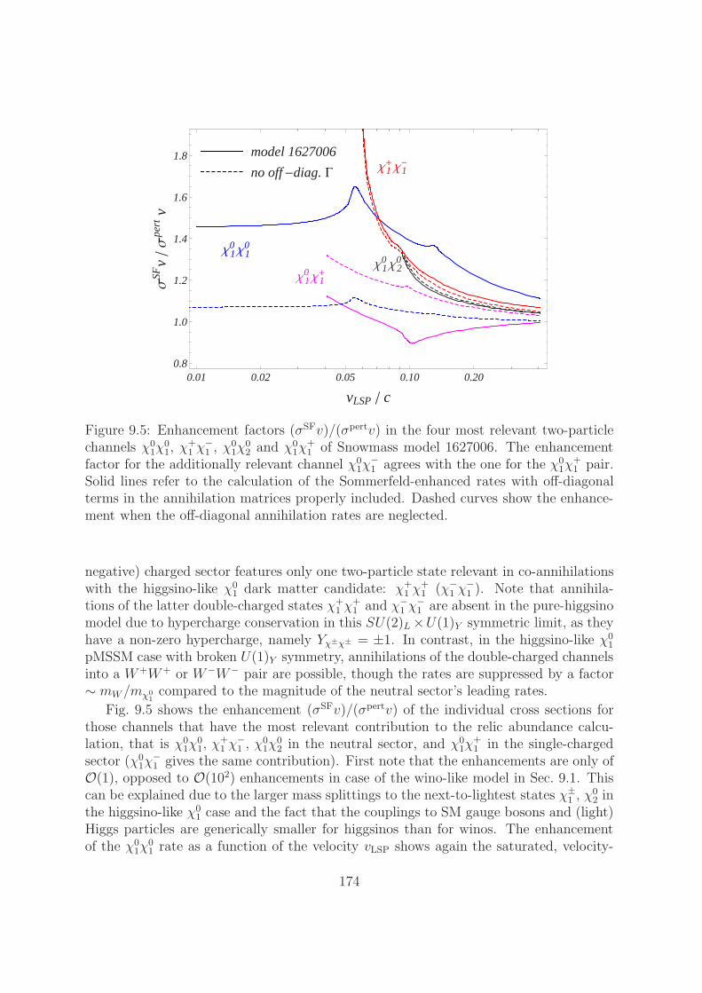
Χ1+Χ1-
Χ10 Χ1
0
Χ10 Χ2
0
Χ10 Χ1+
0.01 0.02 0.05 0.10 0.200.8
1.0
1.2
1.4
1.6
1.8
vLSP c
ΣSF
vΣ
pert
vmodel 1627006
no off-diag. G
Figure 9.5: Enhancement factors (σSFv)/(σpertv) in the four most relevant two-particlechannels χ0
1χ01, χ
+1 χ
−1 , χ
01χ
02 and χ0
1χ+1 of Snowmass model 1627006. The enhancement
factor for the additionally relevant channel χ01χ
−1 agrees with the one for the χ0
1χ+1 pair.
Solid lines refer to the calculation of the Sommerfeld-enhanced rates with off-diagonalterms in the annihilation matrices properly included. Dashed curves show the enhance-ment when the off-diagonal annihilation rates are neglected.
negative) charged sector features only one two-particle state relevant in co-annihilationswith the higgsino-like χ0
1 dark matter candidate: χ+1 χ
+1 (χ−
1 χ−1 ). Note that annihila-
tions of the latter double-charged states χ+1 χ
+1 and χ−
1 χ−1 are absent in the pure-higgsino
model due to hypercharge conservation in this SU(2)L×U(1)Y symmetric limit, as theyhave a non-zero hypercharge, namely Yχ±χ± = ±1. In contrast, in the higgsino-like χ0
1
pMSSM case with broken U(1)Y symmetry, annihilations of the double-charged channelsinto a W+W+ or W−W− pair are possible, though the rates are suppressed by a factor∼ mW/mχ0
1compared to the magnitude of the neutral sector’s leading rates.
Fig. 9.5 shows the enhancement (σSFv)/(σpertv) of the individual cross sections forthose channels that have the most relevant contribution to the relic abundance calcu-lation, that is χ0
1χ01, χ
+1 χ
−1 , χ
01χ
02 in the neutral sector, and χ0
1χ+1 in the single-charged
sector (χ01χ
−1 gives the same contribution). First note that the enhancements are only of
O(1), opposed to O(102) enhancements in case of the wino-like model in Sec. 9.1. Thiscan be explained due to the larger mass splittings to the next-to-lightest states χ±
1 , χ02 in
the higgsino-like χ01 case and the fact that the couplings to SM gauge bosons and (light)
Higgs particles are generically smaller for higgsinos than for winos. The enhancementof the χ0
1χ01 rate as a function of the velocity vLSP shows again the saturated, velocity-
174
independent behaviour typical for Yukawa type potentials in the low velocity regime wellbelow the thresholds of the heavier two-particle states. As in the wino-model, both theoff-diagonal Yukawa potential and the (diagonal) Coulomb potential in the kinematicallyclosed χ+
1 χ−1 channel contribute here to the actual size of the enhancement. At larger
velocities, two resonance regions at the thresholds for χ+1 χ
−1 and χ0
2χ02 production are
visible (the χ02χ
02 channel opens up at vLSP/c ≃ 0.127; the ratio (σSFv)/(σpertv) for this
channel is very close to 1, and is not shown in Fig. 9.5). One might ask why no resonanceat the χ0
1χ02 threshold is visible in the χ0
1χ01 channel: recall that Fermi-statistics forbids
the χ01χ
01-pair to build the totally symmetric partial-wave configurations 3S1 and
1P1. Incase of unbroken SU(2)L × U(1)Y symmetry it turns out, though, that the χ0
1χ02 pair
can build 3S1 and 1P1 configurations but not 1S0 and 3PJ states. Hence there are nooff-diagonal entries in the neutral potential matrices encoding χ0
1χ01 χ0
1χ02 interactions
in the pure-higgsino limit. Departing from the SU(2) × U(1)Y symmetric limit givesrise to χ0
1χ02 contributions to the enhancement (σSFv)/(σpertv) in the χ0
1χ01 channel that
are however suppressed by (mW/mχ01)3 with respect to the leading contributions; this
explains why no χ01χ
02 threshold effect is visible in Fig. 9.5. Such restrictions due to
non-accessible partial-wave configurations do not exist for the next-to-lightest neutraltwo-particle state χ+
1 χ−1 , and resonances at the thresholds of all co-annihilating neutral
χχ-pairs heavier than the χ+1 χ
−1 are visible in the latter channel in Fig. 9.5. Further-
more, note the 1/vχ+1Coulomb-type enhancement in the χ+
1 χ−1 channel directly above its
threshold caused by potential photon-exchange between the χ+1 and χ−
1 . The Coulombpotential surpasses the potentials from massive gauge boson and Higgs exchange at verysmall velocities in the χ+
1 χ−1 channel, but for moderate velocities both the Coulomb and
the (off-)diagonal Yukawa interactions are relevant. Turning to channel χ01χ
02, the corre-
sponding enhancement (σSFv)/(σpertv) increases as the velocity decreases. In particular,there is no saturation of the enhancement directly above threshold, because the lighterchannels χ0
1χ01 and especially χ+
1 χ−1 are always kinematically open and accessible from
an on-shell χ01χ
02 state via off-diagonal potential interactions.
The ratio (σSFv)/(σpertv) for the charged state χ01χ
+1 that is additionally plotted in
Fig. 9.5 (lowermost magenta line) shows that the Sommerfeld effect can also producecorrections that reduce the perturbative result. For the channel χ0
1χ+1 the negative
correction arises from the interference of amplitudes where, after multiple electroweakand Higgs boson exchanges, the state that annihilates into the light final state particlesis the same as the incoming one, χ0
1χ+1 , with amplitudes where the actual state that
annihilates is χ02χ
+1 . In the EFT formalism such interferences arise from the off-diagonal
annihilation terms χ01χ
+1 → χ0
2χ+1 and χ0
2χ+1 → χ0
1χ+1 , combined with the off-diagonal
potential term for χ01χ
+1 → χ0
2χ+1 . The dashed magenta curve in Fig. 9.5 refers to
the situation where off-diagonal short-distance rates are neglected in the calculation ofthe Sommerfeld enhanced χ0
1χ+1 annihilation cross section. It is nicely seen that the
destructive interference effect disappears in this case and the ratio (σSFv)/(σpertv) isalways positive. The enhancement in the χ0
1χ+1 channel also saturates as its on-shell
production threshold is approached. This should be the case as the χ01χ
+1 channel is
the lightest in the single positive-charged sector, and its behaviour should be similar to
175
the one of the lightest neutral channel, χ01χ
01, directly above threshold. However, such
saturation is not visible in Fig. 9.5 because there we plot the χ01χ
+1 cross section as a
function of vLSP and not as a function of the relative velocity of the channel, related tothe latter by v2 = 2(mχ0
1+mχ+
1)/(mχ0
1mχ+
1)×(mχ0
1v2LSP−2δm).3 Let us also mention that
the dip in the χ01χ
+1 cross section caused by interference effects is located at the velocity
where the other state included in the Schrodinger equation for this charge sector, χ02χ
+1 ,
opens up.As we have already noted in context of the χ0
1χ+1 channel above, the dashed curves
in Fig. 9.5 show the results for the corresponding enhancements of the pMSSM scenario1627006 when off-diagonal annihilation rates are neglected. This disregard would leadto an underestimation of the actual enhancement due to the long-range potential in-teractions of around 30% in the χ0
1χ01 channel. The effect is much milder for the χ0
1χ02
and χ+1 χ
−1 pairs and is explained by the contributions of 3S1 partial-wave annihilations
to the cross sections (absent for the identical particle-pair channel χ01χ
01); off-diagonal
3S1 annihilation rates are suppressed relative to the leading (diagonal) rates by an orderof magnitude, due to destructive interference effects between sfermion and gauge bosonexchange amplitudes. Hence, as off-diagonals play a minor role in 3S1 annihilations,their effect in the spin-averaged cross sections σSFv will also be less pronounced. As theconclusions on the enhancements in case of the pure-higgsino χ0
1 model are similar tothe results in Fig. 9.5 we do not show a corresponding plot here. Let us mention thoughagain, that the hard co-annihilation rates in the pure-higgsino model are a few percentsmaller than in the higgsino-like χ0
1 model. Furthermore, the off-diagonal rates for 3S1
annihilations in the system of χ01χ
02 and χ
+1 χ
−1 states are of the same order of magnitude
as the diagonal ones.Fig. 9.6 shows the thermally averaged effective annihilation rate 〈σeffv〉 as a func-
tion of the inverse scaled temperature x. The lower solid (blue) curve represents theresult using perturbatively calculated rates, while the upper two (red) curves with solidand dashed line style refer to computations with Sommerfeld-enhanced cross sectionsincluding and neglecting off-diagonal annihilation rates, respectively. Again the regionfor x . 10 is unphysical, as the co-annihilating particles’ mean velocities are outside thenon-relativistic regime. Due to larger mass splittings between the higgsino-like neutralinoand chargino states, the decoupling of the heavier states χ±
1 and χ02 takes place already
around x ≃ 103. As can be seen from Fig. 9.6, the Sommerfeld effect enhances the ther-mally averaged effective annihilation cross section by 3% up to 25% with respect to theperturbative result in the region of x around 10− 103 which is most relevant in the relicabundance calculation. The effect of correctly treating off-diagonal annihilation rates ismost essential for large values of x in the range 104− 108, where 〈σeffv〉 would be under-estimated by around 25% if off-diagonals were neglected in the hard annihilation rates.In the region x = 10−103 the effect of off-diagonal rates is also noticeable, leading to anoverestimation of 〈σeffv〉 that reaches 6% if off-diagonal rates are not taken into account.
3If the χ01χ
+1 cross section behaves as σSFv ≃ a + bv2 close to threshold, the saturation is visible
because of the zero slope of this function at v = 0; in terms of vLSP it reads σSFv = a + b′(v2LSP − c),which does not have a zero slope at the threshold of the channel, vLSP =
√c.
176
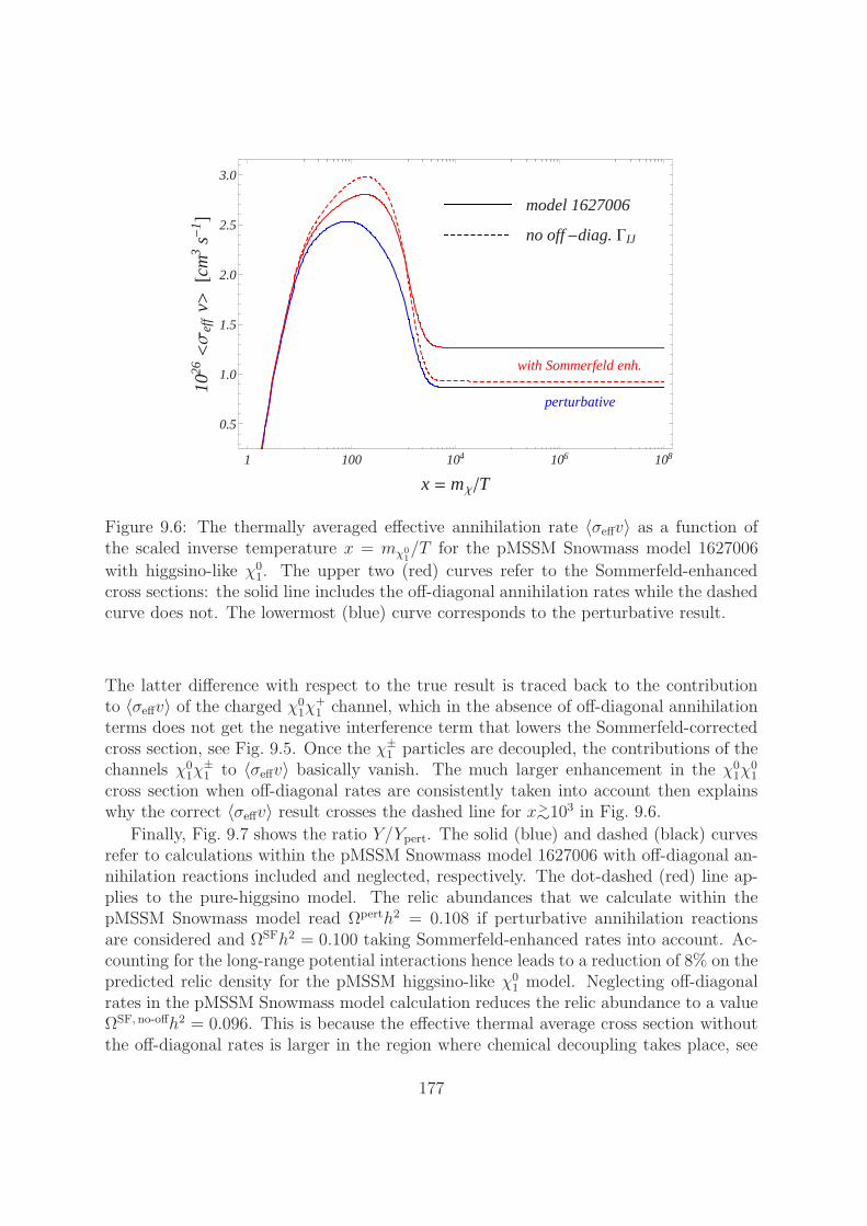
1 100 104 106 108
0.5
1.0
1.5
2.0
2.5
3.0
x = mΧT
1026<Σ
eff
v>@c
m3
s-1 D
model 1627006
no off-diag. GIJ
with Sommerfeld enh.
perturbative
Figure 9.6: The thermally averaged effective annihilation rate 〈σeffv〉 as a function ofthe scaled inverse temperature x = mχ0
1/T for the pMSSM Snowmass model 1627006
with higgsino-like χ01. The upper two (red) curves refer to the Sommerfeld-enhanced
cross sections: the solid line includes the off-diagonal annihilation rates while the dashedcurve does not. The lowermost (blue) curve corresponds to the perturbative result.
The latter difference with respect to the true result is traced back to the contributionto 〈σeffv〉 of the charged χ0
1χ+1 channel, which in the absence of off-diagonal annihilation
terms does not get the negative interference term that lowers the Sommerfeld-correctedcross section, see Fig. 9.5. Once the χ±
1 particles are decoupled, the contributions of thechannels χ0
1χ±1 to 〈σeffv〉 basically vanish. The much larger enhancement in the χ0
1χ01
cross section when off-diagonal rates are consistently taken into account then explainswhy the correct 〈σeffv〉 result crosses the dashed line for x>∼103 in Fig. 9.6.
Finally, Fig. 9.7 shows the ratio Y/Ypert. The solid (blue) and dashed (black) curvesrefer to calculations within the pMSSM Snowmass model 1627006 with off-diagonal an-nihilation reactions included and neglected, respectively. The dot-dashed (red) line ap-plies to the pure-higgsino model. The relic abundances that we calculate within thepMSSM Snowmass model read Ωperth2 = 0.108 if perturbative annihilation reactionsare considered and ΩSFh2 = 0.100 taking Sommerfeld-enhanced rates into account. Ac-counting for the long-range potential interactions hence leads to a reduction of 8% on thepredicted relic density for the pMSSM higgsino-like χ0
1 model. Neglecting off-diagonalrates in the pMSSM Snowmass model calculation reduces the relic abundance to a valueΩSF, no-offh2 = 0.096. This is because the effective thermal average cross section withoutthe off-diagonal rates is larger in the region where chemical decoupling takes place, see
177
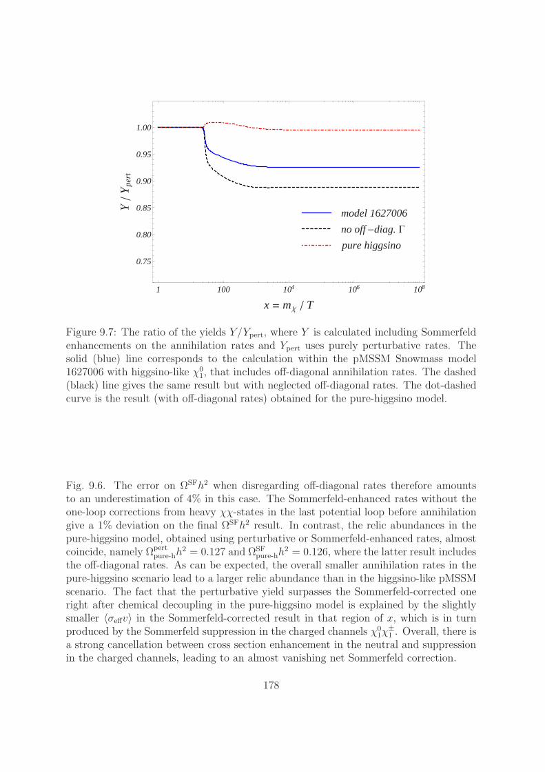
1 100 104 106 108
0.75
0.80
0.85
0.90
0.95
1.00
x = mΧ T
Y
Ype
rt
model 1627006
no off-diag. G
pure higgsino
Figure 9.7: The ratio of the yields Y/Ypert, where Y is calculated including Sommerfeldenhancements on the annihilation rates and Ypert uses purely perturbative rates. Thesolid (blue) line corresponds to the calculation within the pMSSM Snowmass model1627006 with higgsino-like χ0
1, that includes off-diagonal annihilation rates. The dashed(black) line gives the same result but with neglected off-diagonal rates. The dot-dashedcurve is the result (with off-diagonal rates) obtained for the pure-higgsino model.
Fig. 9.6. The error on ΩSFh2 when disregarding off-diagonal rates therefore amountsto an underestimation of 4% in this case. The Sommerfeld-enhanced rates without theone-loop corrections from heavy χχ-states in the last potential loop before annihilationgive a 1% deviation on the final ΩSFh2 result. In contrast, the relic abundances in thepure-higgsino model, obtained using perturbative or Sommerfeld-enhanced rates, almostcoincide, namely Ωpert
pure-hh2 = 0.127 and ΩSF
pure-hh2 = 0.126, where the latter result includes
the off-diagonal rates. As can be expected, the overall smaller annihilation rates in thepure-higgsino scenario lead to a larger relic abundance than in the higgsino-like pMSSMscenario. The fact that the perturbative yield surpasses the Sommerfeld-corrected oneright after chemical decoupling in the pure-higgsino model is explained by the slightlysmaller 〈σeffv〉 in the Sommerfeld-corrected result in that region of x, which is in turnproduced by the Sommerfeld suppression in the charged channels χ0
1χ±1 . Overall, there is
a strong cancellation between cross section enhancement in the neutral and suppressionin the charged channels, leading to an almost vanishing net Sommerfeld correction.
178
9.3 Light scenario
Light neutralino dark matter with a relic abundance of the order of the observed valueis realised for a χ0
1 with a sizable bino component. The bino is a SU(2)L singlet withzero hypercharge. As for a pure bino there are no interactions with electroweak gaugebosons nor photons we can already expect that there will be essentially no long-rangepotential interactions for the bino-like χ0
1 and hence no Sommerfeld enhancements inχ01χ
01 annihilations. Yet it is interesting to confirm this expectation and to investigate
the relevance of Sommerfeld enhancements in possible co-annihilations with (slightly)heavier neutralino and chargino states. As an example for such a bino-like χ0
1 we chose tostudy the pMSSM Snowmass model with ID 2178683 that features wino-like NLSP stateswith masses around 6% heavier than the χ0
1 state: mχ01= 488.8GeV, mχ0
2= 516.0GeV
and mχ+1= 516.2GeV.
In the calculation of the χ01 relic abundance we consider co-annihilation reactions
among all χ0/χ± two-particle states, although only the two-particle annihilations be-tween the states χ0
1,2, χ±1 are relevant since the higgsino-like states χ0
3,4, χ±2 lie at the
2TeV scale and their abundances are strongly Boltzmann-suppressed at χ01 freeze-out.
The lightest sfermions are the τ1 and ντ with masses around 770GeV and we neglecttheir effect in the relic abundance.
Sommerfeld corrections on the co-annihilation cross sections from all two-particlestates built from χ0
1,2 and χ±1 are determined exactly through the solution of the corre-
sponding Schrodinger equations in each charge sector. The outcome for the enhancement(σSFv)/(σpertv) in the neutral sector, which entails the two-particle states χ0
1χ01, χ
01χ
02,
χ02χ
02 and χ+
1 χ−1 , is shown in Fig. 9.8. Solid (dashed) curves correspond to a calculation
with (without) off-diagonal annihilation rates in the Sommerfeld-enhanced reactions.Due to the absence of interactions with the electroweak gauge bosons in case of a pure-bino state, the χ0
1 of the pMSSM Snowmass model 217868 also experiences basically nolong-range potential interactions and there is essentially no coupling between the bino-like χ0
1 and the NLSP χ02. As a consequence, both the absolute (perturbative as well
as Sommerfeld-enhanced) χ01χ
01 and χ0
1χ02 annihilation rates are strongly suppressed and
there is no enhancement in these reactions; the ratio (σSFv)/(σpertv) is equal to one inboth cases. As it cannot be inferred from Fig. 9.8, let us note in addition that the abso-lute χ0
1χ01 (χ0
1χ02) annihilation cross section is suppressed with respect to the dominant
χ02χ
02 and χ+
1 χ−1 rates by four (two) orders of magnitude.
In the subsystem of the neutral wino-like two-particle channels χ02χ
02 and χ+
1 χ−1 , the
Sommerfeld enhancement due to long-range potential interactions is effective, see thecorresponding curves in Fig. 9.8. Note that χ0
2 and χ±1 co-annihilations should still be
relevant in the χ01 relic abundance calculation within the pMSSM scenario 2178683, as
the threshold velocities for χ02χ
02 and χ
+1 χ
−1 on-shell production are vχ0
1
<∼ 0.34 c and thus
of the order of typical χ01 velocities during thermal freeze-out. This scenario provides
an example showing that the criterion established before for including long-distanceeffects among two-particle states with masses smaller than Mmax = 2mχ0
1+mχ0
1v2max and
vmax = 1/3 should not be considered rigidly. Rather it has to be reassessed according to
179

Χ1+Χ1-
Χ10 Χ1
0
Χ10 Χ2
0
Χ20 Χ2
0
0.320 0.325 0.330 0.335 0.340 0.345
1
2
3
4
5
vLSP c
ΣSF
vΣ
pert
vmodel 2178683
no off-diag. G
Figure 9.8: (σSFv)/(σpertv) for the neutral-sector states in the light scenario (Snowmassmodel 2178683). Solid (dashed) curves show the enhancement for the case of properlyincluded (wrongly neglected) off-diagonal annihilation rates.
the given MSSM spectra to avoid overlooking interesting effects. Consequently, in orderto account for the wino-like subsystem formed by the states χ0
2χ02 and χ+
1 χ−1 we have
set vmax = 0.34 in the light scenario. At very small velocities the enhancements in theχ02χ
02 and χ
+1 χ
−1 channels show the characteristics discussed already for the wino model in
Sec. 9.1: In the χ02χ
02 system we find resonances just below the χ+
1 χ−1 threshold, smoothed
out in Fig. 9.8. The strength of the enhancement below and above this resonance regionis a combined effect of the (off-diagonal) Yukawa and the diagonal Coulomb potentialinteractions in the χ+
1 χ−1 system. In particular the enhancement is finite below the χ+
1 χ−1
threshold. To the contrary, the χ+1 χ
−1 channel shows the typical Coulomb-like 1/vχ+
1
enhancement from the dominating photon-exchange potential at velocities directly aboveits on-shell production threshold. Opposed to theO(102) enhancements found in Sec. 9.1,the overall enhancements of the neutral wino-like two-particle channels here reach factorsof O(1) only. These less pronounced enhancements result from the lower masses of thewino-like states, since as mχ0
1decreases the Yukawa potentials from electroweak gauge
boson exchange eventually become short-ranged as compared to the Bohr radius of thesystem proportional to (mχ0
1αEW)−1, where αEW = g22/(4π) and g2 denotes the SU(2)L
gauge coupling.
Fig. 9.9 displays the effective annihilation cross section 〈σeffv〉(x). The dominance ofthe wino-like χ0
2, χ±1 particle annihilation rates by more than three orders of magnitude
before their decoupling near x ∼ 100 is clearly visible. The Sommerfeld enhancementaffects only the annihilation of the wino-like particles and thus disappears for x > 100.
180

1 100 104 106 108
0.01
0.1
1
10
x = mΧT
1026<Σ
eff
v>@c
m3
s-1 D model 2178683
no off-diag. GIJ
with Sommerfeld enh.
pert.
Figure 9.9: The thermally averaged effective rate 〈σeffv〉(x) within the pMSSM Snowmassmodel 2178683 with Sommerfeld enhancements (upper red curve) and in the perturba-tive computation (lower blue curve). The result from disregarding off-diagonal rates inthe Sommerfeld-enhanced processes is plotted by the dashed line. However the lattercurve basically overlays with the upper (red) curve in this plot. This is because theSommerfeld-enhanced 〈σeffv〉(x) is dominated by the χ0
2χ02 and χ+
1 χ−1 rates (before χ0
2
and χ±1 decoupling), and the effect of disregarding off-diagonals in the latter gives a
correction of around 10% only, see Fig. 9.8.
Although the Sommerfeld factors for these channels lead to O(1) enhancements of thecross sections above the threshold near vLSP ∼ 1/3, similar in magnitude to the modelwith wino-like LSP for the same velocities, the thermal average over vLSP dilutes theenhancement, since the cross section for the heavy channels vanishes below the threshold.Nevertheless, the small enhancement visible in Fig. 9.9 occurs precisely in the x rangemost relevant for freeze-out. The effect of co-annihilations with the wino-like NLSPstates therefore leads to a reduction of the yield when taking into account Sommerfeldenhancements with respect to the perturbative case, as is shown in Fig. 9.10. Therelic density with perturbative annihilation rates is found to be Ωperth2 = 0.120. Thereis a ∼ 15% reduction of this result when considering the Sommerfeld-enhanced rates,ΩSFh2 = 0.102. The latter sizable reduction of the relic density is attributed purely tothe co-annihilating heavier wino states. Note that in the sector of wino-like states thepotentials from massive gauge boson and photon exchange are equally important for theSommerfeld enhancement, while in the χ+
1 χ−1 system the Coulomb potential dominates
over the Yukawa potentials only for very small velocities of the charginos. Neglecting
181
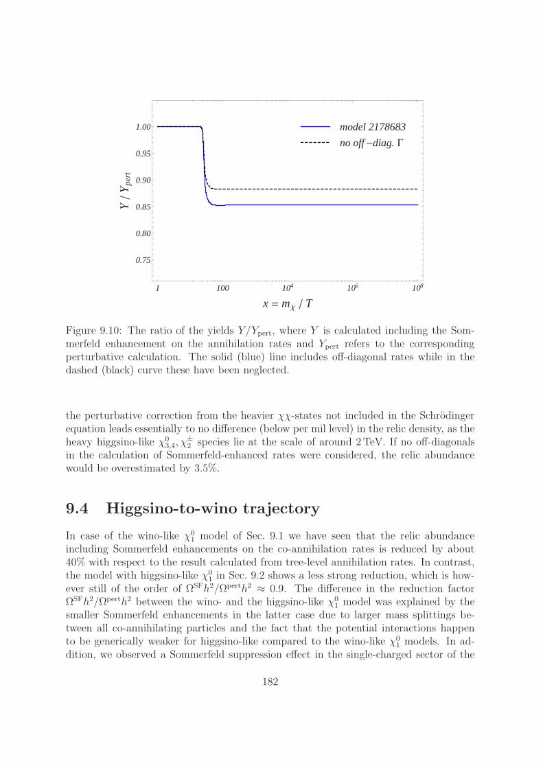
1 100 104 106 108
0.75
0.80
0.85
0.90
0.95
1.00
x = mΧ T
Y
Ype
rtmodel 2178683
no off-diag. G
Figure 9.10: The ratio of the yields Y/Ypert, where Y is calculated including the Som-merfeld enhancement on the annihilation rates and Ypert refers to the correspondingperturbative calculation. The solid (blue) line includes off-diagonal rates while in thedashed (black) curve these have been neglected.
the perturbative correction from the heavier χχ-states not included in the Schrodingerequation leads essentially to no difference (below per mil level) in the relic density, as theheavy higgsino-like χ0
3,4, χ±2 species lie at the scale of around 2TeV. If no off-diagonals
in the calculation of Sommerfeld-enhanced rates were considered, the relic abundancewould be overestimated by 3.5%.
9.4 Higgsino-to-wino trajectory
In case of the wino-like χ01 model of Sec. 9.1 we have seen that the relic abundance
including Sommerfeld enhancements on the co-annihilation rates is reduced by about40% with respect to the result calculated from tree-level annihilation rates. In contrast,the model with higgsino-like χ0
1 in Sec. 9.2 shows a less strong reduction, which is how-ever still of the order of ΩSFh2/Ωperth2 ≈ 0.9. The difference in the reduction factorΩSFh2/Ωperth2 between the wino- and the higgsino-like χ0
1 model was explained by thesmaller Sommerfeld enhancements in the latter case due to larger mass splittings be-tween all co-annihilating particles and the fact that the potential interactions happento be generically weaker for higgsino-like compared to the wino-like χ0
1 models. In ad-dition, we observed a Sommerfeld suppression effect in the single-charged sector of the
182
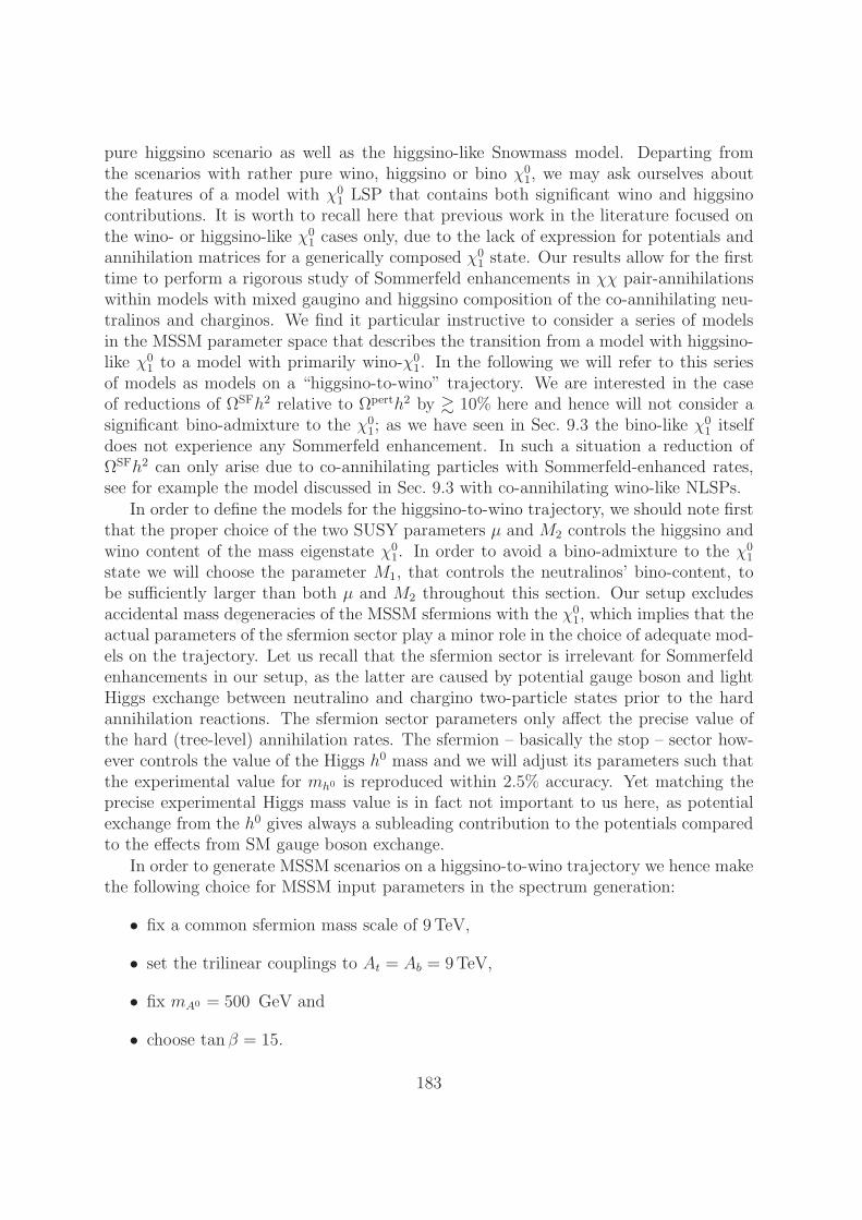
pure higgsino scenario as well as the higgsino-like Snowmass model. Departing fromthe scenarios with rather pure wino, higgsino or bino χ0
1, we may ask ourselves aboutthe features of a model with χ0
1 LSP that contains both significant wino and higgsinocontributions. It is worth to recall here that previous work in the literature focused onthe wino- or higgsino-like χ0
1 cases only, due to the lack of expression for potentials andannihilation matrices for a generically composed χ0
1 state. Our results allow for the firsttime to perform a rigorous study of Sommerfeld enhancements in χχ pair-annihilationswithin models with mixed gaugino and higgsino composition of the co-annihilating neu-tralinos and charginos. We find it particular instructive to consider a series of modelsin the MSSM parameter space that describes the transition from a model with higgsino-like χ0
1 to a model with primarily wino-χ01. In the following we will refer to this series
of models as models on a “higgsino-to-wino” trajectory. We are interested in the caseof reductions of ΩSFh2 relative to Ωperth2 by & 10% here and hence will not consider asignificant bino-admixture to the χ0
1; as we have seen in Sec. 9.3 the bino-like χ01 itself
does not experience any Sommerfeld enhancement. In such a situation a reduction ofΩSFh2 can only arise due to co-annihilating particles with Sommerfeld-enhanced rates,see for example the model discussed in Sec. 9.3 with co-annihilating wino-like NLSPs.
In order to define the models for the higgsino-to-wino trajectory, we should note firstthat the proper choice of the two SUSY parameters µ and M2 controls the higgsino andwino content of the mass eigenstate χ0
1. In order to avoid a bino-admixture to the χ01
state we will choose the parameter M1, that controls the neutralinos’ bino-content, tobe sufficiently larger than both µ and M2 throughout this section. Our setup excludesaccidental mass degeneracies of the MSSM sfermions with the χ0
1, which implies that theactual parameters of the sfermion sector play a minor role in the choice of adequate mod-els on the trajectory. Let us recall that the sfermion sector is irrelevant for Sommerfeldenhancements in our setup, as the latter are caused by potential gauge boson and lightHiggs exchange between neutralino and chargino two-particle states prior to the hardannihilation reactions. The sfermion sector parameters only affect the precise value ofthe hard (tree-level) annihilation rates. The sfermion – basically the stop – sector how-ever controls the value of the Higgs h0 mass and we will adjust its parameters such thatthe experimental value for mh0 is reproduced within 2.5% accuracy. Yet matching theprecise experimental Higgs mass value is in fact not important to us here, as potentialexchange from the h0 gives always a subleading contribution to the potentials comparedto the effects from SM gauge boson exchange.
In order to generate MSSM scenarios on a higgsino-to-wino trajectory we hence makethe following choice for MSSM input parameters in the spectrum generation:
• fix a common sfermion mass scale of 9 TeV,
• set the trilinear couplings to At = Ab = 9TeV,
• fix mA0 = 500 GeV and
• choose tan β = 15.
183

All other trilinear couplings are assumed to vanish. The gluino mass parameter M3
is fixed by M3 = αs/(sin(θw)αe)M2, but this choice is completely irrelevant to ourdiscussion. To avoid a significant bino-admixture to the χ0
1 we further restrict to modelswith M1 = 10M2. This leaves us with yet-to-choose parameter pairs in the µ − M2
plane. We require that the trajectory models allow for an explanation of the observedcosmic cold dark matter in terms of the neutralino relic abundance without includingradiative corrections: in order to do so we employ the program DarkSUSY [5] and identify(µ,M2) pairs such that the DarkSUSY calculated relic density ΩDSh2 matches the mostaccurate determination obtained from the combination of PLANCK, WMAP, BAO andhigh resolution CMB data, Ωcdmh
2 = 0.1187 ± 0.0017 [2]4, which we quoted already inChap. 1. In such a way we define 13 models on the higgsino-to-wino trajectory. Theposition of these models in the µ −M2 plane is shown in Fig. 9.11. For each of the 13models, given the pairs (µ,M2) as well as the remaining input parameters defined above,we run our code and determine the corresponding relic densities including and neglectingSommerfeld effects. The comparison between our perturbative results Ωperth2 with thecorresponding DarkSUSY expressions ΩDSh2 provides a cross-check of our perturbativecalculation.
There is one important point to note concerning the MSSM spectrum generationfrom the SUSY input parameters. The DarkSUSY spectrum calculated from the in-puts refers to tree-level DR-parameters. It is well-known and has been noted before inChap. 4 that the mass splitting between a wino-like neutralino and its chargino partneris dominated by radiative corrections; the leading one-loop contribution to the splittingis of O(160MeV) and dominates over the O(1MeV) tree-level contribution. Both for thecalculation of the Sommerfeld enhancements and in the determination of the relic abun-dance including co-annihilations a precise knowledge of the mass splitting between theχ01 LSP and the NLSP particles is crucial and in a rigorous analysis we should therefore
consider the spectra determined with one-loop accuracy. To this end we have been pro-vided by one-loop on-shell renormalised SUSY spectra for all 13 models on the trajectoryby a member of the collaboration [83,84]. The values of the input parameters µ,M2, . . .are the same as for the corresponding calculation within DarkSUSY with the differencethat for the one-loop on-shell spectrum generation these inputs are considered as on-shellparameters and no renormalisation group running of the mass parameters is performed.Hence there are small differences in the values for the masses and mixing-matrix en-tries between the spectra that we use in our code and the corresponding DarkSUSYspectra. In particular the mass splittings between the χ0
1 LSP and the NLSPs obtainedfrom the on-shell masses renormalised at one-loop can be significantly different from thesplittings derived using tree-level DR-parameters. There exist different renormalisationschemes for on-shell renormalisation in the neutralino/chargino sector [82–85]: for alltrajectory models apart from model 8 the on-shell renormalisation has been performedrequiring that the values of the two chargino masses as well as the heaviest (in all ourmodels bino-like) neutralino mass at one-loop are given by their tree-level values (“CCN-
4Note that the DarkSUSY collaboration claims an error of 5% on the relic densities calculated fromtheir code.
184

ì
ì
ì
ì
ìì
ì
ì
ì
ì ì ì ì
1000 1500 2000 2500 3000 35001000
1500
2000
2500
3000
3500
Μ
M2
1
2
3
4
5 67
8
9 10 11 12 13
Wh2 = 0.3Wh2 = 0.15Wh2 = 0.1187Wh2 = 0.095
Figure 9.11: The µ−M2 plane with the 13 models defining the higgsino-to-wino trajec-tory, indicated with diamonds. All trajectory models lie on the iso-contour for constantrelic density ΩDSh2 = 0.1187 calculated with DarkSUSY. As reference we also show theiso-contours of constant relic densities ΩDSh2 = 0.095 (lowermost contour-line) 0.15 and0.3 (uppermost iso-contour).
scheme”). Such a scheme works well as long as the two charginos are rather pure wino-and higgsino-like states. As soon as the charginos are (strongly) mixed wino-higgsinostates - as in case of our model 8, where the input parameters µ and M2 happen to bevery close to each other - a more suitable scheme is obtained when only one chargino, onelighter neutralino and the heaviest bino-like neutralino mass are fixed to their tree-levelvalue (“CNN scheme”).
For each of the 13 models on the trajectory we list the input parameters µ and M2
in Tab. 9.1, together with the one-loop renormalised LSP mass mχ01as well as the one-
loop on-shell mass splitting δmχ+1= mχ+
1− mχ0
1. The χ±
1 is the NLSP in all models
considered in this section. As additional information we give the χ01’s wino fraction
|ZN 21|2 and collect the results for ΩSFh2 including Sommerfeld effects as well as for thesuppression ΩSFh2/Ωperth2 of the former relic density with respect to the perturbative
185
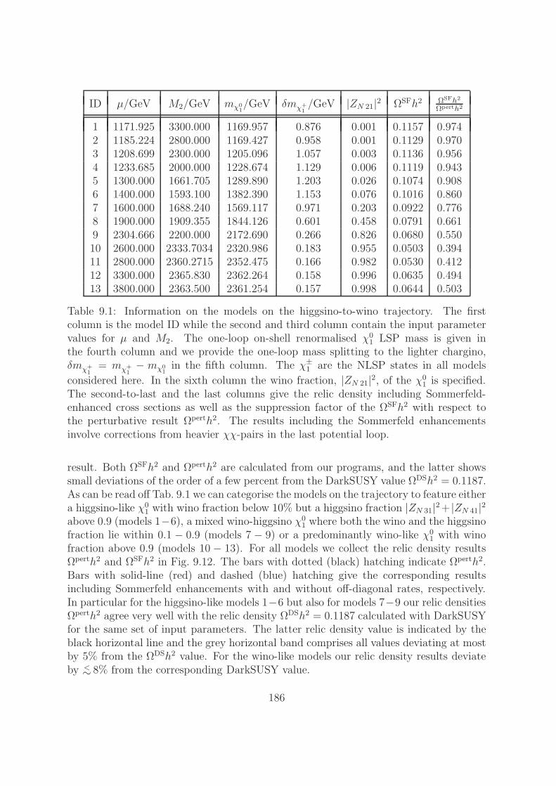
ID µ/GeV M2/GeV mχ01/GeV δmχ+
1/GeV |ZN 21|2 ΩSFh2 ΩSFh2
Ωperth2
1 1171.925 3300.000 1169.957 0.876 0.001 0.1157 0.9742 1185.224 2800.000 1169.427 0.958 0.001 0.1129 0.9703 1208.699 2300.000 1205.096 1.057 0.003 0.1136 0.9564 1233.685 2000.000 1228.674 1.129 0.006 0.1119 0.9435 1300.000 1661.705 1289.890 1.203 0.026 0.1074 0.9086 1400.000 1593.100 1382.390 1.153 0.076 0.1016 0.8607 1600.000 1688.240 1569.117 0.971 0.203 0.0922 0.7768 1900.000 1909.355 1844.126 0.601 0.458 0.0791 0.6619 2304.666 2200.000 2172.690 0.266 0.826 0.0680 0.55010 2600.000 2333.7034 2320.986 0.183 0.955 0.0503 0.39411 2800.000 2360.2715 2352.475 0.166 0.982 0.0530 0.41212 3300.000 2365.830 2362.264 0.158 0.996 0.0635 0.49413 3800.000 2363.500 2361.254 0.157 0.998 0.0644 0.503
Table 9.1: Information on the models on the higgsino-to-wino trajectory. The firstcolumn is the model ID while the second and third column contain the input parametervalues for µ and M2. The one-loop on-shell renormalised χ0
1 LSP mass is given inthe fourth column and we provide the one-loop mass splitting to the lighter chargino,δmχ+
1= mχ+
1− mχ0
1in the fifth column. The χ±
1 are the NLSP states in all models
considered here. In the sixth column the wino fraction, |ZN 21|2, of the χ01 is specified.
The second-to-last and the last columns give the relic density including Sommerfeld-enhanced cross sections as well as the suppression factor of the ΩSFh2 with respect tothe perturbative result Ωperth2. The results including the Sommerfeld enhancementsinvolve corrections from heavier χχ-pairs in the last potential loop.
result. Both ΩSFh2 and Ωperth2 are calculated from our programs, and the latter showssmall deviations of the order of a few percent from the DarkSUSY value ΩDSh2 = 0.1187.As can be read off Tab. 9.1 we can categorise the models on the trajectory to feature eithera higgsino-like χ0
1 with wino fraction below 10% but a higgsino fraction |ZN 31|2+ |ZN 41|2above 0.9 (models 1−6), a mixed wino-higgsino χ0
1 where both the wino and the higgsinofraction lie within 0.1 − 0.9 (models 7 − 9) or a predominantly wino-like χ0
1 with winofraction above 0.9 (models 10 − 13). For all models we collect the relic density resultsΩperth2 and ΩSFh2 in Fig. 9.12. The bars with dotted (black) hatching indicate Ωperth2.Bars with solid-line (red) and dashed (blue) hatching give the corresponding resultsincluding Sommerfeld enhancements with and without off-diagonal rates, respectively.In particular for the higgsino-like models 1−6 but also for models 7−9 our relic densitiesΩperth2 agree very well with the relic density ΩDSh2 = 0.1187 calculated with DarkSUSYfor the same set of input parameters. The latter relic density value is indicated by theblack horizontal line and the grey horizontal band comprises all values deviating at mostby 5% from the ΩDSh2 value. For the wino-like models our relic density results deviateby <∼ 8% from the corresponding DarkSUSY value.
186
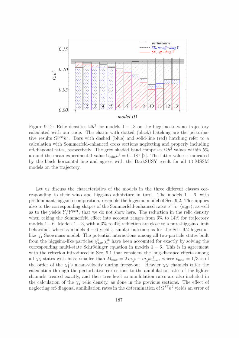
Figure 9.12: Relic densities Ωh2 for models 1 − 13 on the higgsino-to-wino trajectorycalculated with our code. The charts with dotted (black) hatching are the perturba-tive results Ωperth2. Bars with dashed (blue) and solid-line (red) hatching refer to acalculation with Sommerfeld-enhanced cross sections neglecting and properly includingoff-diagonal rates, respectively. The grey shaded band comprises Ωh2 values within 5%around the mean experimental value Ωcdmh
2 = 0.1187 [2]. The latter value is indicatedby the black horizontal line and agrees with the DarkSUSY result for all 13 MSSMmodels on the trajectory.
Let us discuss the characteristics of the models in the three different classes cor-responding to their wino and higgsino admixture in turn. The models 1 − 6, withpredominant higgsino composition, resemble the higgsino model of Sec. 9.2. This appliesalso to the corresponding shapes of the Sommerfeld-enhanced rates σSFv, 〈σeffv〉, as wellas to the yields Y/Y pert, that we do not show here. The reduction in the relic densitywhen taking the Sommerfeld effect into account ranges from 3% to 14% for trajectorymodels 1−6. Models 1−3, with a 3% to 4% reduction are close to a pure-higgsino limitbehaviour, whereas models 4 − 6 yield a similar outcome as for the Sec. 9.2 higgsino-like χ0
1 Snowmass model. The potential interactions among all two-particle states builtfrom the higgsino-like particles χ0
1,2, χ±1 have been accounted for exactly by solving the
corresponding multi-state Schrodinger equation in models 1 − 6. This is in agreementwith the criterion introduced in Sec. 9.1 that considers the long-distance effects amongall χχ-states with mass smaller than Mmax = 2mχ0
1+mχ0
1v2max, where vmax = 1/3 is of
the order of the χ01’s mean-velocity during freeze-out. Heavier χχ channels enter the
calculation through the perturbative corrections to the annihilation rates of the lighterchannels treated exactly, and their tree-level co-annihilation rates are also included inthe calculation of the χ0
1 relic density, as done in the previous sections. The effect ofneglecting off-diagonal annihilation rates in the determination of ΩSFh2 yields an error of
187
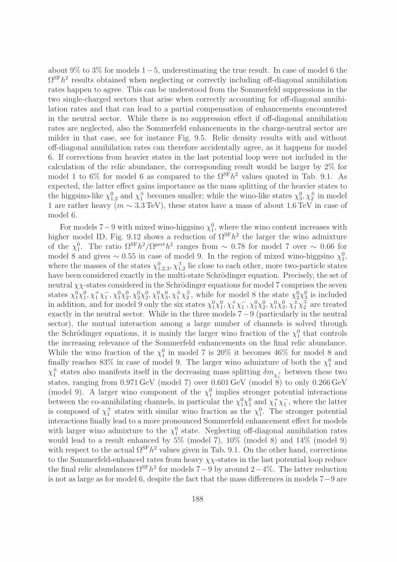
about 9% to 3% for models 1−5, underestimating the true result. In case of model 6 theΩSFh2 results obtained when neglecting or correctly including off-diagonal annihilationrates happen to agree. This can be understood from the Sommerfeld suppressions in thetwo single-charged sectors that arise when correctly accounting for off-diagonal annihi-lation rates and that can lead to a partial compensation of enhancements encounteredin the neutral sector. While there is no suppression effect if off-diagonal annihilationrates are neglected, also the Sommerfeld enhancements in the charge-neutral sector aremilder in that case, see for instance Fig. 9.5. Relic density results with and withoutoff-diagonal annihilation rates can therefore accidentally agree, as it happens for model6. If corrections from heavier states in the last potential loop were not included in thecalculation of the relic abundance, the corresponding result would be larger by 2% formodel 1 to 6% for model 6 as compared to the ΩSFh2 values quoted in Tab. 9.1. Asexpected, the latter effect gains importance as the mass splitting of the heavier states tothe higgsino-like χ0
1,2 and χ±1 becomes smaller; while the wino-like states χ0
3, χ±2 in model
1 are rather heavy (m ∼ 3.3TeV), these states have a mass of about 1.6TeV in case ofmodel 6.
For models 7−9 with mixed wino-higgsino χ01, where the wino content increases with
higher model ID, Fig. 9.12 shows a reduction of ΩSFh2 the larger the wino admixtureof the χ0
1. The ratio ΩSFh2/Ωperth2 ranges from ∼ 0.78 for model 7 over ∼ 0.66 formodel 8 and gives ∼ 0.55 in case of model 9. In the region of mixed wino-higgsino χ0
1,where the masses of the states χ0
1,2,3, χ±1,2 lie close to each other, more two-particle states
have been considered exactly in the multi-state Schrodinger equation. Precisely, the set ofneutral χχ-states considered in the Schrodinger equations for model 7 comprises the sevenstates χ0
1χ01, χ
+1 χ
−1 , χ
01χ
02, χ
02χ
02, χ
01χ
03, χ
±1 χ
∓2 , while for model 8 the state χ0
2χ03 is included
in addition, and for model 9 only the six states χ01χ
01, χ
+1 χ
−1 , χ
01χ
02, χ
01χ
03, χ
±1 χ
∓2 are treated
exactly in the neutral sector. While in the three models 7−9 (particularly in the neutralsector), the mutual interaction among a large number of channels is solved throughthe Schrodinger equations, it is mainly the larger wino fraction of the χ0
1 that controlsthe increasing relevance of the Sommerfeld enhancements on the final relic abundance.While the wino fraction of the χ0
1 in model 7 is 20% it becomes 46% for model 8 andfinally reaches 83% in case of model 9. The larger wino admixture of both the χ0
1 andχ±1 states also manifests itself in the decreasing mass splitting δmχ+
1between these two
states, ranging from 0.971GeV (model 7) over 0.601GeV (model 8) to only 0.266GeV(model 9). A larger wino component of the χ0
1 implies stronger potential interactionsbetween the co-annihilating channels, in particular the χ0
1χ01 and χ
+1 χ
−1 , where the latter
is composed of χ±1 states with similar wino fraction as the χ0
1. The stronger potentialinteractions finally lead to a more pronounced Sommerfeld enhancement effect for modelswith larger wino admixture to the χ0
1 state. Neglecting off-diagonal annihilation rateswould lead to a result enhanced by 5% (model 7), 10% (model 8) and 14% (model 9)with respect to the actual ΩSFh2 values given in Tab. 9.1. On the other hand, correctionsto the Sommerfeld-enhanced rates from heavy χχ-states in the last potential loop reducethe final relic abundances ΩSFh2 for models 7−9 by around 2−4%. The latter reductionis not as large as for model 6, despite the fact that the mass differences in models 7−9 are
188
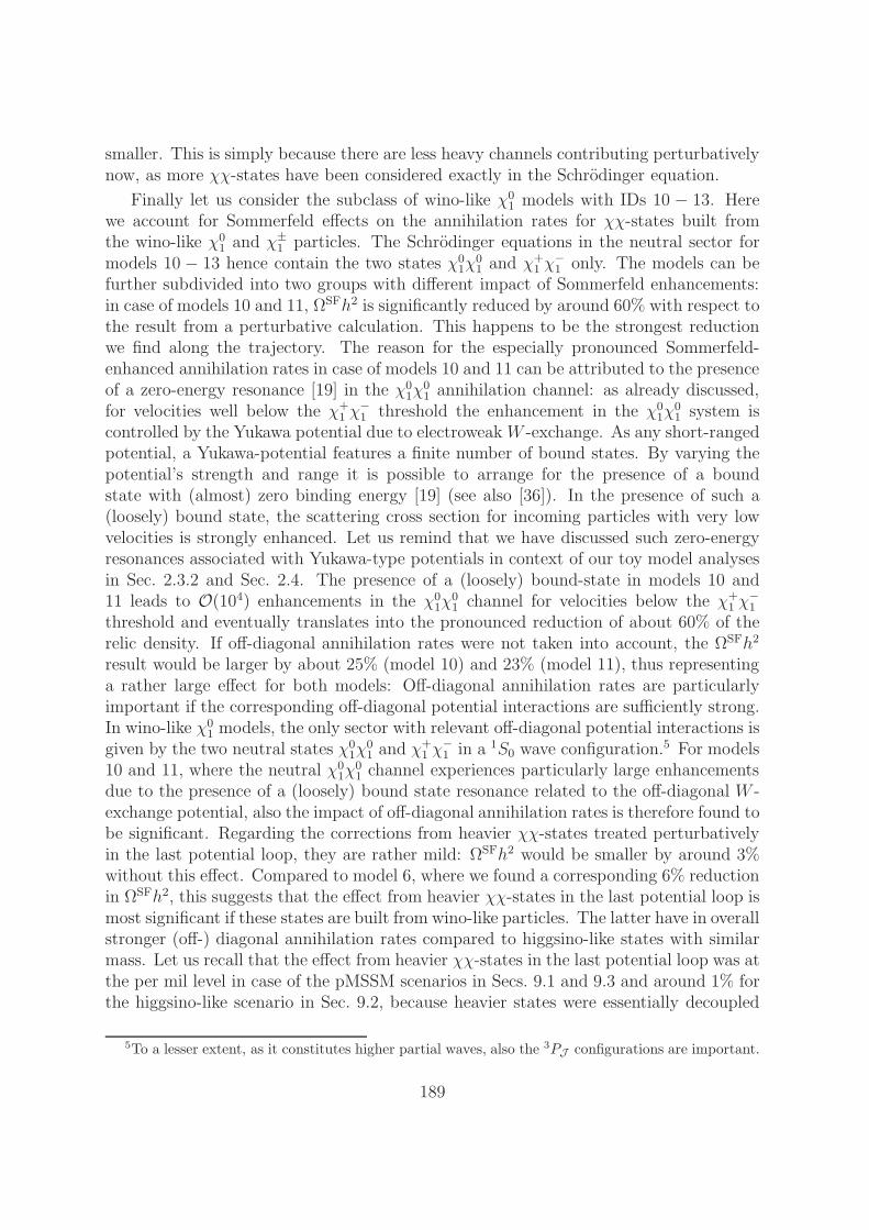
smaller. This is simply because there are less heavy channels contributing perturbativelynow, as more χχ-states have been considered exactly in the Schrodinger equation.
Finally let us consider the subclass of wino-like χ01 models with IDs 10 − 13. Here
we account for Sommerfeld effects on the annihilation rates for χχ-states built fromthe wino-like χ0
1 and χ±1 particles. The Schrodinger equations in the neutral sector for
models 10 − 13 hence contain the two states χ01χ
01 and χ+
1 χ−1 only. The models can be
further subdivided into two groups with different impact of Sommerfeld enhancements:in case of models 10 and 11, ΩSFh2 is significantly reduced by around 60% with respect tothe result from a perturbative calculation. This happens to be the strongest reductionwe find along the trajectory. The reason for the especially pronounced Sommerfeld-enhanced annihilation rates in case of models 10 and 11 can be attributed to the presenceof a zero-energy resonance [19] in the χ0
1χ01 annihilation channel: as already discussed,
for velocities well below the χ+1 χ
−1 threshold the enhancement in the χ0
1χ01 system is
controlled by the Yukawa potential due to electroweakW -exchange. As any short-rangedpotential, a Yukawa-potential features a finite number of bound states. By varying thepotential’s strength and range it is possible to arrange for the presence of a boundstate with (almost) zero binding energy [19] (see also [36]). In the presence of such a(loosely) bound state, the scattering cross section for incoming particles with very lowvelocities is strongly enhanced. Let us remind that we have discussed such zero-energyresonances associated with Yukawa-type potentials in context of our toy model analysesin Sec. 2.3.2 and Sec. 2.4. The presence of a (loosely) bound-state in models 10 and11 leads to O(104) enhancements in the χ0
1χ01 channel for velocities below the χ+
1 χ−1
threshold and eventually translates into the pronounced reduction of about 60% of therelic density. If off-diagonal annihilation rates were not taken into account, the ΩSFh2
result would be larger by about 25% (model 10) and 23% (model 11), thus representinga rather large effect for both models: Off-diagonal annihilation rates are particularlyimportant if the corresponding off-diagonal potential interactions are sufficiently strong.In wino-like χ0
1 models, the only sector with relevant off-diagonal potential interactions isgiven by the two neutral states χ0
1χ01 and χ
+1 χ
−1 in a 1S0 wave configuration.
5 For models10 and 11, where the neutral χ0
1χ01 channel experiences particularly large enhancements
due to the presence of a (loosely) bound state resonance related to the off-diagonal W -exchange potential, also the impact of off-diagonal annihilation rates is therefore found tobe significant. Regarding the corrections from heavier χχ-states treated perturbativelyin the last potential loop, they are rather mild: ΩSFh2 would be smaller by around 3%without this effect. Compared to model 6, where we found a corresponding 6% reductionin ΩSFh2, this suggests that the effect from heavier χχ-states in the last potential loop ismost significant if these states are built from wino-like particles. The latter have in overallstronger (off-) diagonal annihilation rates compared to higgsino-like states with similarmass. Let us recall that the effect from heavier χχ-states in the last potential loop was atthe per mil level in case of the pMSSM scenarios in Secs. 9.1 and 9.3 and around 1% forthe higgsino-like scenario in Sec. 9.2, because heavier states were essentially decoupled
5To a lesser extent, as it constitutes higher partial waves, also the 3PJ configurations are important.
189
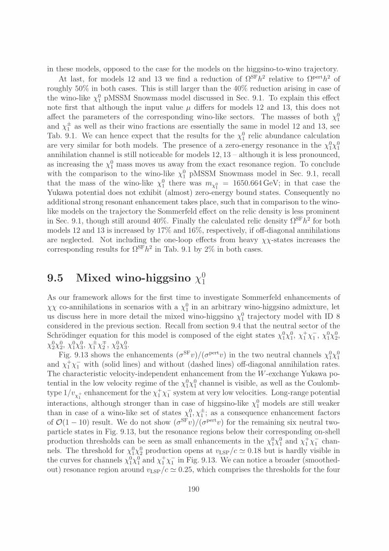
in these models, opposed to the case for the models on the higgsino-to-wino trajectory.
At last, for models 12 and 13 we find a reduction of ΩSFh2 relative to Ωperth2 ofroughly 50% in both cases. This is still larger than the 40% reduction arising in case ofthe wino-like χ0
1 pMSSM Snowmass model discussed in Sec. 9.1. To explain this effectnote first that although the input value µ differs for models 12 and 13, this does notaffect the parameters of the corresponding wino-like sectors. The masses of both χ0
1
and χ±1 as well as their wino fractions are essentially the same in model 12 and 13, see
Tab. 9.1. We can hence expect that the results for the χ01 relic abundance calculation
are very similar for both models. The presence of a zero-energy resonance in the χ01χ
01
annihilation channel is still noticeable for models 12, 13 – although it is less pronounced,as increasing the χ0
1 mass moves us away from the exact resonance region. To concludewith the comparison to the wino-like χ0
1 pMSSM Snowmass model in Sec. 9.1, recallthat the mass of the wino-like χ0
1 there was mχ01= 1650.664GeV; in that case the
Yukawa potential does not exhibit (almost) zero-energy bound states. Consequently noadditional strong resonant enhancement takes place, such that in comparison to the wino-like models on the trajectory the Sommerfeld effect on the relic density is less prominentin Sec. 9.1, though still around 40%. Finally the calculated relic density ΩSFh2 for bothmodels 12 and 13 is increased by 17% and 16%, respectively, if off-diagonal annihilationsare neglected. Not including the one-loop effects from heavy χχ-states increases thecorresponding results for ΩSFh2 in Tab. 9.1 by 2% in both cases.
9.5 Mixed wino-higgsino χ01
As our framework allows for the first time to investigate Sommerfeld enhancements ofχχ co-annihilations in scenarios with a χ0
1 in an arbitrary wino-higgsino admixture, letus discuss here in more detail the mixed wino-higgsino χ0
1 trajectory model with ID 8considered in the previous section. Recall from section 9.4 that the neutral sector of theSchrodinger equation for this model is composed of the eight states χ0
1χ01, χ
+1 χ
−1 , χ
01χ
02,
χ02χ
02, χ
01χ
03, χ
±1 χ
∓2 , χ
02χ
03.
Fig. 9.13 shows the enhancements (σSFv)/(σpertv) in the two neutral channels χ01χ
01
and χ+1 χ
−1 with (solid lines) and without (dashed lines) off-diagonal annihilation rates.
The characteristic velocity-independent enhancement from the W -exchange Yukawa po-tential in the low velocity regime of the χ0
1χ01 channel is visible, as well as the Coulomb-
type 1/vχ+1enhancement for the χ+
1 χ−1 system at very low velocities. Long-range potential
interactions, although stronger than in case of higgsino-like χ01 models are still weaker
than in case of a wino-like set of states χ01, χ
±1 ; as a consequence enhancement factors
of O(1 − 10) result. We do not show (σSFv)/(σpertv) for the remaining six neutral two-particle states in Fig. 9.13, but the resonance regions below their corresponding on-shellproduction thresholds can be seen as small enhancements in the χ0
1χ01 and χ+
1 χ−1 chan-
nels. The threshold for χ01χ
02 production opens at vLSP/c ≃ 0.18 but is hardly visible in
the curves for channels χ01χ
01 and χ
+1 χ
−1 in Fig. 9.13. We can notice a broader (smoothed-
out) resonance region around vLSP/c ≃ 0.25, which comprises the thresholds for the four
190

Χ1+Χ1-
Χ10Χ1
0
0.001 0.005 0.010 0.050 0.100
1.0
10.0
5.0
2.0
20.0
3.0
1.5
15.0
7.0
vLSP c
ΣSF
vΣ
pert
vmodel 8no off-diag. G
pure-Coulomb enh.
Figure 9.13: Enhancements (σSFv)/(σpertv) in the two neutral channels χ01χ
01 and χ+
1 χ−1
of model 8 of the wino-to-higgsino trajectory discussed in Sec. 9.4. Solid (dashed) curvesrefer to the results with (without) off-diagonal annihilation rates included.
channels χ02χ
02, χ
01χ
03 and χ±
1 χ∓2 . Finally, the χ0
2χ03 threshold shows up at vLSP/c ≃ 0.30.
The enhancements for these channels, not shown in Fig. 9.13, are somewhat smaller thanfor the cases of χ0
1χ01 and χ+
1 χ−1 . Eventually, at vLSP/c ≃ 0.35 the threshold for on-shell
production of the χ03χ
03 state is visible in the χ+
1 χ−1 channel. The χ0
3χ03 state is among
the heavy states considered perturbatively in the last potential loop for the calculationof the annihilation rates of the channels treated exactly in the neutral sector.
Note that apart from the bino-like χ04 state, which is very heavy (mχ0
4∼ 19 TeV) and
– being bino-like – couples very weakly to the gauge bosons and the other χ0/χ± species,all χ states in the neutralino/chargino sector are relevant in co-annihilation reactions forthe χ0
1 relic abundance calculation of model 8.
The thermally averaged effective annihilation rates 〈σeffv〉(x) including (upper solid(red) line) and neglecting (dashed red line) off-diagonal rates in the Sommerfeld-enhancedcross sections are depicted in the upper panel of Fig. 9.14. The corresponding perturba-tive result is given by the lower solid (blue) curve. The perturbative annihilation rates oftwo-particle states χχ heavier than the χ0
1χ01 pair are larger than the perturbative rate of
the latter, leading to a drop in the perturbative 〈σeffv〉(x) curve after decoupling of theheavier co-annihilating χχ states. As can be already inferred from Fig. 9.13, the effectiverate including Sommerfeld enhancements turns out to be larger than the correspondingperturbative result by factors of at most O(1− 3) in the x range x = 10 . . . 103 relevantto the relic abundance calculation. These enhancements finally give rise to the behaviourof the ratio of yields Y/Ypert shown in the lower panel of Fig. 9.14. Including Sommerfeld
191
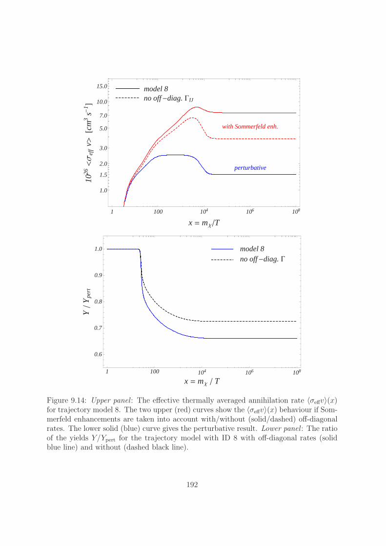
1 100 104 106 108
1.0
10.0
5.0
2.0
3.0
1.5
15.0
7.0
x = mΧT
1026<Σ
eff
v>@c
m3
s-1 D
model 8no off-diag. GIJ
with Sommerfeld enh.
perturbative
1 100 104 106 108
0.6
0.7
0.8
0.9
1.0
x = mΧ T
Y
Ype
rt
model 8no off-diag. G
Figure 9.14: Upper panel : The effective thermally averaged annihilation rate 〈σeffv〉(x)for trajectory model 8. The two upper (red) curves show the 〈σeffv〉(x) behaviour if Som-merfeld enhancements are taken into account with/without (solid/dashed) off-diagonalrates. The lower solid (blue) curve gives the perturbative result. Lower panel : The ratioof the yields Y/Ypert for the trajectory model with ID 8 with off-diagonal rates (solidblue line) and without (dashed black line).
192
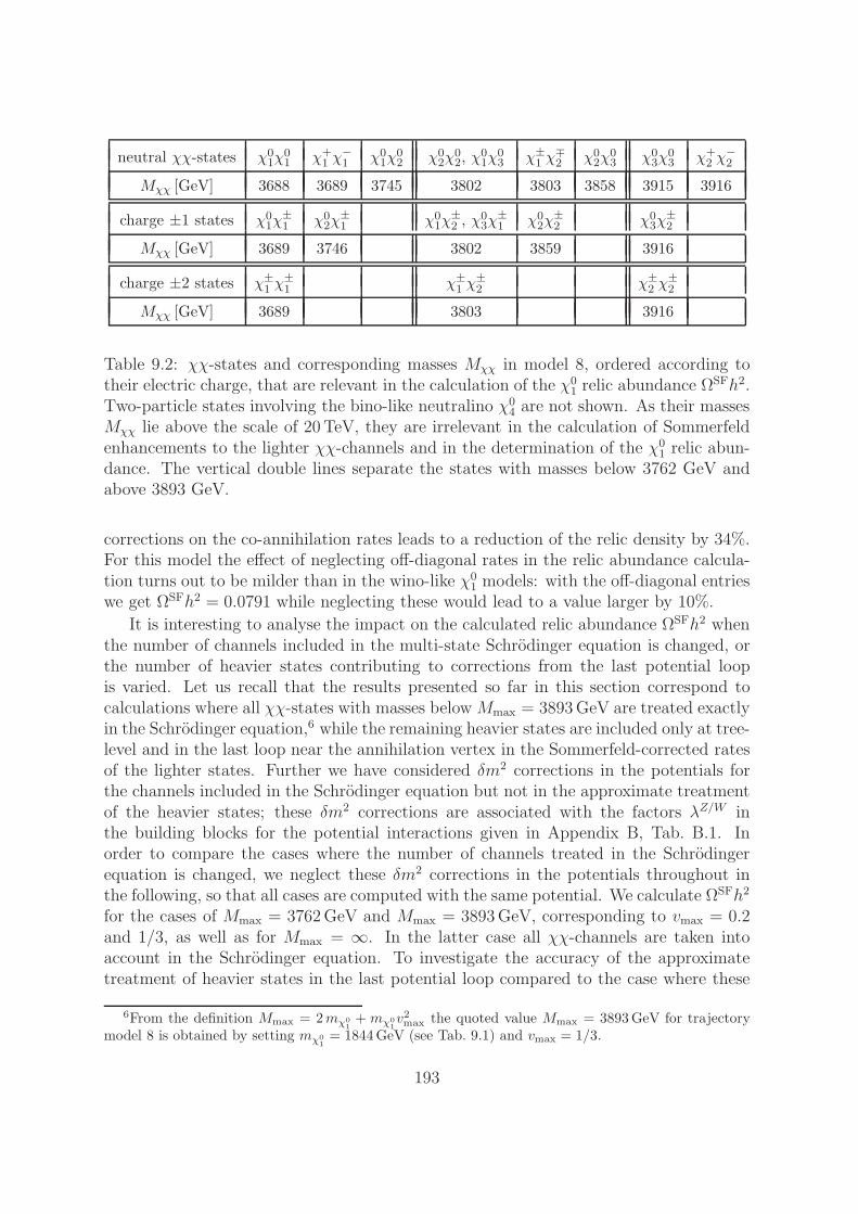
neutral χχ-states χ01χ
01 χ+
1 χ−1 χ0
1χ02 χ0
2χ02, χ
01χ
03 χ±
1 χ∓2 χ0
2χ03 χ0
3χ03 χ+
2 χ−2
Mχχ [GeV] 3688 3689 3745 3802 3803 3858 3915 3916
charge ±1 states χ01χ
±1 χ0
2χ±1 χ0
1χ±2 , χ
03χ
±1 χ0
2χ±2 χ0
3χ±2
Mχχ [GeV] 3689 3746 3802 3859 3916
charge ±2 states χ±1 χ
±1 χ±
1 χ±2 χ±
2 χ±2
Mχχ [GeV] 3689 3803 3916
Table 9.2: χχ-states and corresponding masses Mχχ in model 8, ordered according totheir electric charge, that are relevant in the calculation of the χ0
1 relic abundance ΩSFh2.
Two-particle states involving the bino-like neutralino χ04 are not shown. As their masses
Mχχ lie above the scale of 20TeV, they are irrelevant in the calculation of Sommerfeldenhancements to the lighter χχ-channels and in the determination of the χ0
1 relic abun-dance. The vertical double lines separate the states with masses below 3762 GeV andabove 3893 GeV.
corrections on the co-annihilation rates leads to a reduction of the relic density by 34%.For this model the effect of neglecting off-diagonal rates in the relic abundance calcula-tion turns out to be milder than in the wino-like χ0
1 models: with the off-diagonal entrieswe get ΩSFh2 = 0.0791 while neglecting these would lead to a value larger by 10%.
It is interesting to analyse the impact on the calculated relic abundance ΩSFh2 whenthe number of channels included in the multi-state Schrodinger equation is changed, orthe number of heavier states contributing to corrections from the last potential loopis varied. Let us recall that the results presented so far in this section correspond tocalculations where all χχ-states with masses belowMmax = 3893GeV are treated exactlyin the Schrodinger equation,6 while the remaining heavier states are included only at tree-level and in the last loop near the annihilation vertex in the Sommerfeld-corrected ratesof the lighter states. Further we have considered δm2 corrections in the potentials forthe channels included in the Schrodinger equation but not in the approximate treatmentof the heavier states; these δm2 corrections are associated with the factors λZ/W inthe building blocks for the potential interactions given in Appendix B, Tab. B.1. Inorder to compare the cases where the number of channels treated in the Schrodingerequation is changed, we neglect these δm2 corrections in the potentials throughout inthe following, so that all cases are computed with the same potential. We calculate ΩSFh2
for the cases of Mmax = 3762GeV and Mmax = 3893GeV, corresponding to vmax = 0.2and 1/3, as well as for Mmax = ∞. In the latter case all χχ-channels are taken intoaccount in the Schrodinger equation. To investigate the accuracy of the approximatetreatment of heavier states in the last potential loop compared to the case where these
6From the definition Mmax = 2mχ01+mχ0
1v2max the quoted value Mmax = 3893GeV for trajectory
model 8 is obtained by setting mχ01= 1844GeV (see Tab. 9.1) and vmax = 1/3.
193
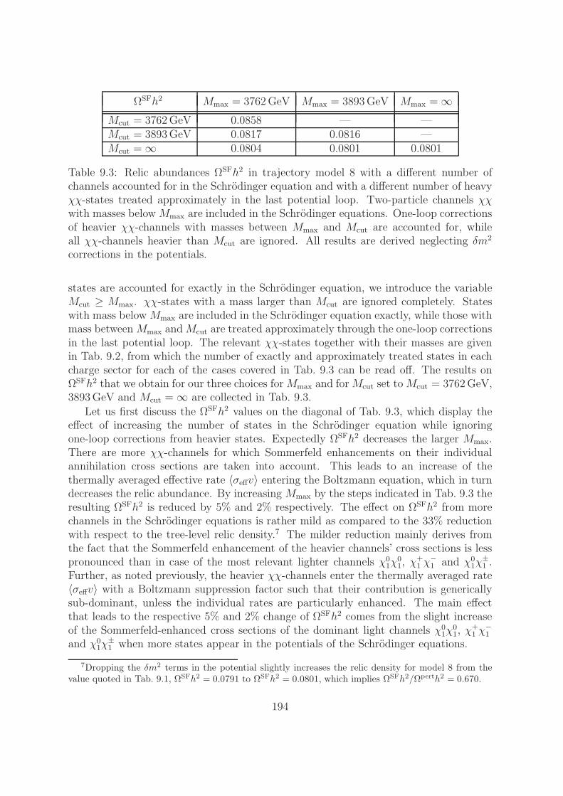
ΩSFh2 Mmax = 3762GeV Mmax = 3893GeV Mmax =∞Mcut = 3762GeV 0.0858 — —Mcut = 3893GeV 0.0817 0.0816 —Mcut =∞ 0.0804 0.0801 0.0801
Table 9.3: Relic abundances ΩSFh2 in trajectory model 8 with a different number ofchannels accounted for in the Schrodinger equation and with a different number of heavyχχ-states treated approximately in the last potential loop. Two-particle channels χχwith masses belowMmax are included in the Schrodinger equations. One-loop correctionsof heavier χχ-channels with masses between Mmax and Mcut are accounted for, whileall χχ-channels heavier than Mcut are ignored. All results are derived neglecting δm2
corrections in the potentials.
states are accounted for exactly in the Schrodinger equation, we introduce the variableMcut ≥ Mmax. χχ-states with a mass larger than Mcut are ignored completely. Stateswith mass belowMmax are included in the Schrodinger equation exactly, while those withmass betweenMmax andMcut are treated approximately through the one-loop correctionsin the last potential loop. The relevant χχ-states together with their masses are givenin Tab. 9.2, from which the number of exactly and approximately treated states in eachcharge sector for each of the cases covered in Tab. 9.3 can be read off. The results onΩSFh2 that we obtain for our three choices forMmax and forMcut set toMcut = 3762GeV,3893GeV and Mcut =∞ are collected in Tab. 9.3.
Let us first discuss the ΩSFh2 values on the diagonal of Tab. 9.3, which display theeffect of increasing the number of states in the Schrodinger equation while ignoringone-loop corrections from heavier states. Expectedly ΩSFh2 decreases the larger Mmax.There are more χχ-channels for which Sommerfeld enhancements on their individualannihilation cross sections are taken into account. This leads to an increase of thethermally averaged effective rate 〈σeffv〉 entering the Boltzmann equation, which in turndecreases the relic abundance. By increasing Mmax by the steps indicated in Tab. 9.3 theresulting ΩSFh2 is reduced by 5% and 2% respectively. The effect on ΩSFh2 from morechannels in the Schrodinger equations is rather mild as compared to the 33% reductionwith respect to the tree-level relic density.7 The milder reduction mainly derives fromthe fact that the Sommerfeld enhancement of the heavier channels’ cross sections is lesspronounced than in case of the most relevant lighter channels χ0
1χ01, χ
+1 χ
−1 and χ0
1χ±1 .
Further, as noted previously, the heavier χχ-channels enter the thermally averaged rate〈σeffv〉 with a Boltzmann suppression factor such that their contribution is genericallysub-dominant, unless the individual rates are particularly enhanced. The main effectthat leads to the respective 5% and 2% change of ΩSFh2 comes from the slight increaseof the Sommerfeld-enhanced cross sections of the dominant light channels χ0
1χ01, χ
+1 χ
−1
and χ01χ
±1 when more states appear in the potentials of the Schrodinger equations.
7Dropping the δm2 terms in the potential slightly increases the relic density for model 8 from thevalue quoted in Tab. 9.1, ΩSFh2 = 0.0791 to ΩSFh2 = 0.0801, which implies ΩSFh2/Ωperth2 = 0.670.
194
Let us now consider the reduction of ΩSFh2 for fixed Mmax and increasing Mcut. Thishappens because the effect of heavier channels amounts to a positive correction to theSommerfeld-enhanced cross sections: the dominant potential interactions are attractive,such that the heavier states in the last potential loop typically give an additional positivecontribution. For instance we find a significant reduction of ΩSFh2 by 5% from 0.858to 0.817, when for Mmax = 3762GeV the value of Mcut is increased from 3762GeV to3893GeV. This indicates that the newly added heavier states in the last loop give alarge positive contribution to the Sommerfeld-enhanced cross sections of the χχ-statesin the Schrodinger equation. When CPU considerations make the restriction to fewerstates treated in the Schrodinger equation necessary, the approximate treatment of heavychannels should give a reasonable approximation to the case where these heavy channelsare included fully in the Schrodinger equation. This is nicely confirmed by the num-bers shown in Tab.9.3: when the states with mass between 3762GeV and 3893GeVare treated approximately, the reduction of ΩSFh2 from 0.0858 to 0.0817 is very closeto the value 0.0816 obtained from the exact treatment of all states with mass below3893GeV. The same observation holds for the comparison between the approximatetreatment of all states with masses above 3762GeV, ΩSFh2 = 0.0804, and the exactresult ΩSFh2 = 0.0801. The agreement becomes even better when the the perturbativetreatment involves only the heavier channels with mass above 3893GeV.
195

196
Chapter 10
Conclusions
We have studied the impact of Sommerfeld enhancements on co-annihilation rates of non-relativistic and nearly mass-degenerate heavy neutralino and chargino pairs, consideringin particular the effect on the χ0
1 relic abundance calculation.
For a systematic investigation in the general MSSM, where the χ01 is an arbitrary
admixture of the electroweak-eigenstate gauginos and higgsinos, we have constructed anon-relativistic effective field theory, the NRMSSM, that is designed to calculate theenhanced radiative corrections to pair-annihilation rates of close-in-mass neutralino andchargino states with small relative velocities. The NRMSSM shares similarities with theNRQCD framework applied to heavy quarkonium annihilation. An important differenceis the presence of several heavy neutralino and chargino species with small mass differ-ences in the NRMSSM in contrast to a single heavy quark together with its anti-quark inNRQCD. Further, massive mediator exchange occurs among the heavy neutralino andchargino NRMSSM states, where the mediator particles are given by the electroweakgauge bosons, the photon and the light Higgs bosons subject to the underlying MSSMspectrum. Apart from the photon, which is associated with diagonal Coulomb-type po-tentials, the mediator particles generate diagonal as well as off-diagonal Yukawa-typepotential interactions that allow for potential scattering transitions between two close-in-mass particle pairs built from the NRMSSM neutralino and chargino states.
In the NRMSSM the neutralino and chargino co-annihilation cross sections are ob-tained from the imaginary part of scattering matrix elements of four-fermion operators.Factorisation of short-distance and long-range effects in the annihilation processes is au-tomatically provided in the effective theory: the short-distance annihilation is encodedin the absorptive parts of the Wilson coefficients of the four-fermion operators, whilethe matrix-elements of the latter operators contain the long-range effects causing theSommerfeld enhancements of the full annihilation rate. The weak coupling nature ofthe involved electromagnetic and electroweak potential interactions allows to explicitlycalculate the matrix elements of the four-fermion operators.
Due to the presence of off-diagonal potentials, the NRMSSM short-distance annihila-tion reactions are characterised by diagonal as well as off-diagonal rates. We have derivedpurely analytical expressions for all such (off-) diagonal non-relativistic annihilation rates
197

up to corrections of O(v2rel) and at leading order in the expansion in couplings. The di-agonal rates thus reproduce the tree-level annihilation cross sections of non-relativisticneutralino and chargino pairs including the O(v2rel) P - and next-to-next-to-leading orderS-wave effects. We have performed a dedicated comparison of our results to numericaldata for the pair-annihilation rates obtained with the code MadGraph, showing a goodreliability of our non-relativistic approximation up to relative velocities of vrel ≃ 0.4 c.Our comprehensive results for the (off-) diagonal NRMSSM annihilation rates extendpreviously known expressions in several aspects. First, off-diagonal short-distance ratesin Sommerfeld-enhanced annihilation reactions were only consistently included in thesimple limiting scenarios of pure wino and pure higgsino χ0
1. Further, the effect of Som-merfeld enhancements on P - and next-to-next-to-leading order S-wave rates has notbeen considered before. It is worth to mention that a partial-wave separation of theshort-distance rates, which is needed for a consistent treatment of the partial-wave de-pendent Sommerfeld enhancements, is obtained in the NRMSSM by construction, inparticular disentangling the O(v2rel) short distance P - and next-to-next-to-leading orderS-wave rates.
As regards the potential interactions, we have presented analytic results for all (off-)diagonal leading-order potentials between the NRMSSM neutralino and chargino states,accounting for electroweak gauge boson as well as light Higgs boson exchange. A centralexpression in our NRMSSM framework is formula (8.13) that gives the Sommerfeld-corrected annihilation rate of a pair χiχj of NRMSSM states including O(v2rel) correctionsin the short-distance part; it generalises the non-relativistic approximation to the tree-level annihilation cross section, σχiχj
vrel = a+b v2rel, by taking Sommerfeld enhancementsinto account.
The determination of the partial-wave dependent Sommerfeld enhancement factorsrequires the solution of a multi-state Schrodinger equation containing potential matricesthat are related to the (off-) diagonal potential interactions among the NRMSSM states.We have described a novel method to solve the Schrodinger equation in order to obtainthe Sommerfeld factors, that is free from numerical instabilities associated with thepresence of kinematically closed heavier two-particle channels. In addition we havesuggested an approximate treatment of very heavy two-particle states, which are notpart of the set of NRMSSM neutralinos and charginos: by introduction of appropriateeffective short-distance rates, certain heavy-channel contributions to the annihilationreactions of the NRMSSM states can be incorporated.
As application of our effective theory framework we have presented a detailed inves-tigation of Sommerfeld enhancements in the χ0
1 relic abundance calculation for severalbenchmark models with heavy neutralino LSP in the general MSSM. Our analysis is fo-cused on three pMSSM benchmark models with wino-, higgsino- and bino-like χ0
1 takenfrom [98]. Since our framework allows for the first time a consistent investigation ofSommerfeld enhancements in neutralino/chargino co-annihilations for χ0
1 states with ar-bitrary gaugino and higgsino mixture, we have additionally defined a “higgsino-to-wino”trajectory in the parameter space of the general MSSM. This trajectory is given by a setof 13 DarkSUSY generated spectra interpolating between the cases of a higgsino- to a
198
wino-like χ01 spectrum. In scenarios with wino-like χ0
1 we have found sizable 40% to 60%reductions of the relic density when accounting for Sommerfeld-enhanced co-annihilationrates with respect to the calculation with corresponding perturbative cross sections. Thereduction is found to be much milder, of the order of 3% to 14%, in case of the studiedhiggsino-like χ0
1 models. These results are in agreement with previous investigations inthe literature in the pure-wino and pure-higgsino limits. In general the relic abundanceobtained including the Sommerfeld effect is reduced the more the stronger the wino ad-mixture to the χ0
1. Cases of particular pronounced effects are related to the existence ofloosely or zero-energy bound states in the spectrum of the corresponding model. Ourinvestigations show that the precise value of the calculated relic density depends onthe particular details of the spectrum, such that results from a study in the pure-winoor pure-higgsino χ0
1 scenarios do not apply directly. Interestingly, the Sommerfeld en-hancements in the co-annihilating sector of a bino-like χ0
1 can affect the result on ΩSFh2
at the 10% level, which is found for the studied benchmark model with bino-like χ01
and slightly heavier wino-like χ±/χ0 states. The knowledge of precise mass splittingsbetween the co-annihilating neutralinos and charginos is essential in the calculation ofSommerfeld-enhanced rates and will typically require the knowledge of spectra with aone-loop on-shell renormalised neutralino/chargino sector.
With the analyses of Sommerfeld enhancements in neutralino/chargino co-annihilationsin several MSSM scenarios we have shown the general features of the enhancement ef-fect and its particular relevance regarding the neutralino relic abundance calculation.Our results imply that Sommerfeld enhancements have to be taken into account whenderiving MSSM parameter space constraints on heavy neutralino dark matter from acombination of direct and indirect dark matter searches, collider constraints and theadditional requirement to reproduce or at least not overproduce the observed cosmicdark matter abundance in terms of a χ0
1 relic. Our effective theory framework allows forcorresponding future investigations of the parameter space of the general MSSM in viewof the relevance of Sommerfeld enhancements in the χ0
1 relic abundance calculation.It is worth to stress that the NRMSSM that we have developed in this thesis provides
the first – and at the moment the only available – technique to account for Sommerfeldenhancements in neutralino and chargino co-annihilations in the general MSSM witharbitrary χ0
1 composition. The method can be extended to other WIMP dark mattermodels provided the necessary model-dependent inputs, that is the potential and anni-hilation matrices, are known.
199

200
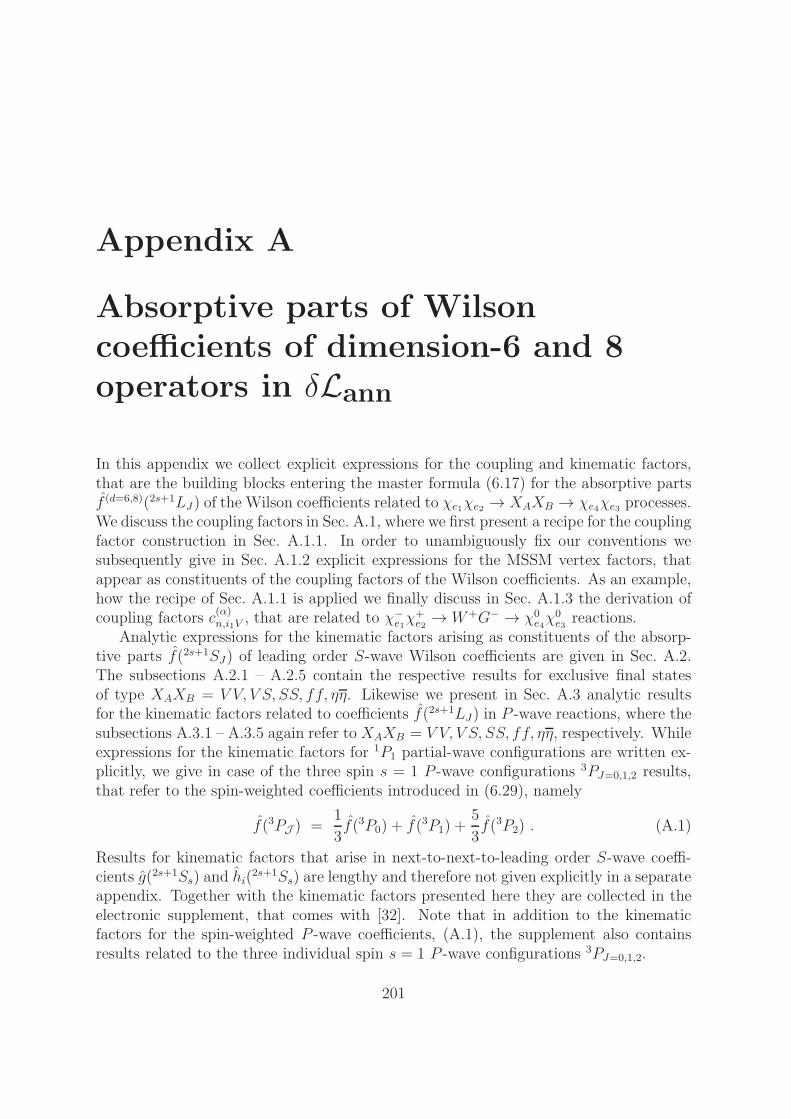
Appendix A
Absorptive parts of Wilsoncoefficients of dimension-6 and 8operators in δLann
In this appendix we collect explicit expressions for the coupling and kinematic factors,that are the building blocks entering the master formula (6.17) for the absorptive partsf (d=6,8)(2s+1LJ ) of the Wilson coefficients related to χe1χe2 → XAXB → χe4χe3 processes.We discuss the coupling factors in Sec. A.1, where we first present a recipe for the couplingfactor construction in Sec. A.1.1. In order to unambiguously fix our conventions wesubsequently give in Sec. A.1.2 explicit expressions for the MSSM vertex factors, thatappear as constituents of the coupling factors of the Wilson coefficients. As an example,how the recipe of Sec. A.1.1 is applied we finally discuss in Sec. A.1.3 the derivation ofcoupling factors c
(α)n,i1V
, that are related to χ−e1χ+e2→W+G− → χ0
e4χ0e3
reactions.Analytic expressions for the kinematic factors arising as constituents of the absorp-
tive parts f(2s+1SJ) of leading order S-wave Wilson coefficients are given in Sec. A.2.The subsections A.2.1 – A.2.5 contain the respective results for exclusive final statesof type XAXB = V V, V S, SS, ff, ηη. Likewise we present in Sec. A.3 analytic resultsfor the kinematic factors related to coefficients f(2s+1LJ) in P -wave reactions, where thesubsections A.3.1 – A.3.5 again refer to XAXB = V V, V S, SS, ff, ηη, respectively. Whileexpressions for the kinematic factors for 1P1 partial-wave configurations are written ex-plicitly, we give in case of the three spin s = 1 P -wave configurations 3PJ=0,1,2 results,that refer to the spin-weighted coefficients introduced in (6.29), namely
f(3PJ ) =1
3f(3P0) + f(3P1) +
5
3f(3P2) . (A.1)
Results for kinematic factors that arise in next-to-next-to-leading order S-wave coeffi-cients g(2s+1Ss) and hi(
2s+1Ss) are lengthy and therefore not given explicitly in a separateappendix. Together with the kinematic factors presented here they are collected in theelectronic supplement, that comes with [32]. Note that in addition to the kinematicfactors for the spin-weighted P -wave coefficients, (A.1), the supplement also containsresults related to the three individual spin s = 1 P -wave configurations 3PJ=0,1,2.
201
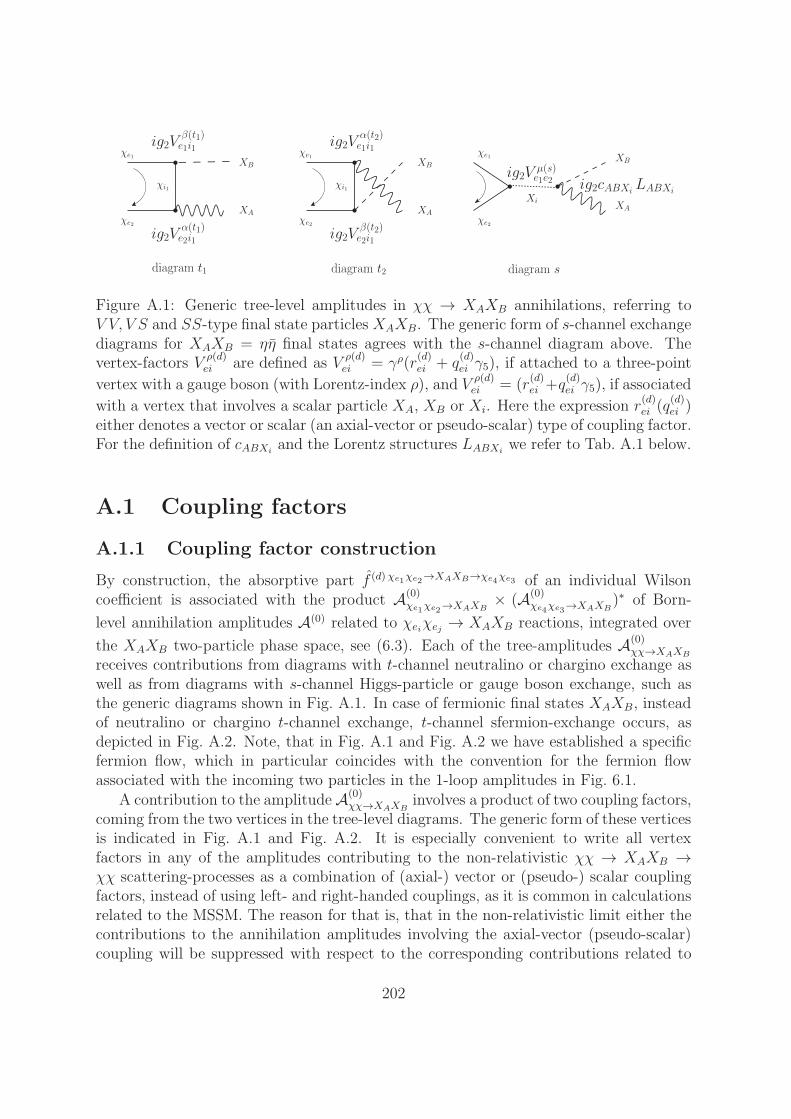
ig2Vµ(s)e1e2
ig2Vα(t1)e2i1
ig2Vβ(t1)e1i1
XA
XBXBXB
XAXA
ig2Vβ(t2)e2i1
ig2Vα(t2)e1i1
diagram t1 diagram t2 diagram s
χe1
χe2
χi1 χi1
χe1
χe2
χe1
χe2
Xi
ig2cABXi LABXi
Figure A.1: Generic tree-level amplitudes in χχ → XAXB annihilations, referring toV V, V S and SS-type final state particles XAXB. The generic form of s-channel exchangediagrams for XAXB = ηη final states agrees with the s-channel diagram above. Thevertex-factors V
ρ(d)ei are defined as V
ρ(d)ei = γρ(r
(d)ei + q
(d)ei γ5), if attached to a three-point
vertex with a gauge boson (with Lorentz-index ρ), and Vρ(d)ei = (r
(d)ei +q
(d)ei γ5), if associated
with a vertex that involves a scalar particle XA, XB or Xi. Here the expression r(d)ei (q
(d)ei )
either denotes a vector or scalar (an axial-vector or pseudo-scalar) type of coupling factor.For the definition of cABXi
and the Lorentz structures LABXiwe refer to Tab. A.1 below.
A.1 Coupling factors
A.1.1 Coupling factor construction
By construction, the absorptive part f (d)χe1χe2
→XAXB→χe4χe3 of an individual Wilson
coefficient is associated with the product A(0)χe1
χe2→XAXB
× (A(0)χe4
χe3→XAXB
)∗ of Born-
level annihilation amplitudes A(0) related to χeiχej → XAXB reactions, integrated over
the XAXB two-particle phase space, see (6.3). Each of the tree-amplitudes A(0)χχ→XAXB
receives contributions from diagrams with t-channel neutralino or chargino exchange aswell as from diagrams with s-channel Higgs-particle or gauge boson exchange, such asthe generic diagrams shown in Fig. A.1. In case of fermionic final states XAXB, insteadof neutralino or chargino t-channel exchange, t-channel sfermion-exchange occurs, asdepicted in Fig. A.2. Note, that in Fig. A.1 and Fig. A.2 we have established a specificfermion flow, which in particular coincides with the convention for the fermion flowassociated with the incoming two particles in the 1-loop amplitudes in Fig. 6.1.
A contribution to the amplitudeA(0)χχ→XAXB
involves a product of two coupling factors,coming from the two vertices in the tree-level diagrams. The generic form of these verticesis indicated in Fig. A.1 and Fig. A.2. It is especially convenient to write all vertexfactors in any of the amplitudes contributing to the non-relativistic χχ → XAXB →χχ scattering-processes as a combination of (axial-) vector or (pseudo-) scalar couplingfactors, instead of using left- and right-handed couplings, as it is common in calculationsrelated to the MSSM. The reason for that is, that in the non-relativistic limit either thecontributions to the annihilation amplitudes involving the axial-vector (pseudo-scalar)coupling will be suppressed with respect to the corresponding contributions related to
202
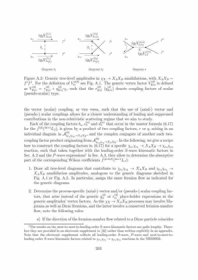
ig2V(t1)Ie2i1
ig2V(t1)Je1i1
f I
fJfJfJ
f If I
ig2V(t2)Je2i1
ig2V(t2)Ie1i1
diagram t1 diagram t2 diagram s
χe1
χe2
Si1 Si1
χe1
χe2
χe1
χe2
Xi
ig2Vµ(s)e1e2
ig2Vν(s)IJ
Figure A.2: Generic tree-level amplitudes in χχ → XAXB annihilations, with XAXB =f IfJ . For the definition of V
ρ(d)ei see Fig. A.1. The generic vertex factor V
(d)Kei is defined
as V(d)Kei = r
(d)Kei + q
(d)Keiγ5, such that the r
(d)Kei (q
(d)Kei) denote coupling factors of scalar
(pseudo-scalar) type.
the vector (scalar) coupling, or vice versa, such that the use of (axial-) vector and(pseudo-) scalar couplings allows for a clearer understanding of leading and suppressedcontributions in the non-relativistic scattering regime that we aim to study.
Each of the coupling factors bn, c(α)n and d
(α)n that occur in the master formula (6.17)
for the f (d)(2s+1LJ ), is given by a product of two coupling factors, r or q, arising in an
individual diagram in A(0)χe1
χe2→XAXB
, and the complex conjugate of another such two-
coupling factor product originating fromA(0)χe4
χe3→XAXB
. In the following, we give a recipe
how to construct the coupling factors in (6.17) for a specific χe1χe2 → XAXB → χe4χe3reaction, such that taken together with the leading-order S-wave kinematic factors inSec. A.2 and the P -wave expressions1 in Sec. A.3, they allow to determine the absorptivepart of the corresponding Wilson coefficients f (d=6,8)(2s+1LJ ):
1. Draw all tree-level diagrams that contribute to χe1χe2 → XAXB and χe4χe3 →XAXB annihilation amplitudes, analogous to the generic diagrams sketched inFig. A.1 or Fig. A.2. In particular, assign the same fermion flow as indicated forthe generic diagrams.
2. Determine the process-specific (axial-) vector and/or (pseudo-) scalar coupling fac-
tors, that arise instead of the generic q(d)ei or r
(d)ei place-holder expressions at the
generic amplitudes’ vertex factors. As the χχ→ XAXB processes may involve Ma-jorana as well as Dirac fermions, and the latter involve a conserved fermion-numberflow, note the following rules:
a) If the direction of the fermion-number flow related to a Dirac particle coincides
1The results on the next-to-next-to-leading order S-wave kinematic factors are quite lengthy. There-fore they are provided in an electronic supplement to [32] rather than written explicitly in an appendix.Note that the electronic supplement collects all leading-order S-wave, P -wave and next-to-next-to-leading order S-wave kinematic factors related to χe1χe2 → χe4χe3 reactions in the NRMSSM.
203
with the direction of the fermion flow (fixed as in Fig. A.1 and Fig. A.2), theχχ → XAXB process specific coupling factors at the vertices are directly de-duced from the corresponding interaction terms in the underlying Lagrangian.These coupling factors are given later in (A.4–A.10).
b) Otherwise, if the fermion-number flow is antiparallel to the indicated fermionflow, vector coupling factors at vertices attached to a Dirac fermion line, aregiven by a factor−1 times the expression for the vector coupling given in (A.4–A.6). Axial-vector, scalar and pseudo-scalar coupling factors are unchangedwith respect to case a) above.
3. Build all possible two-coupling factor products, including possible signs related tovector couplings, as far as the case in 2b) above applies, that can arise in eachsingle diagram.
4. Multiply each of the two-coupling factor products, that arise in the A(0)χe1
χe2→XAXB
amplitude, with the complex conjugate of each of the two-coupling factor products,arising in A(0)
χe4χe3
→XAXB. As a result, all possible coupling factor combinations that
can occur in f (d=6,8)χe1χe2
→XAXB→χe4χe3 are obtained.
Rule 2b) arises in the following way for the case of diagram s in Figs. A.1-A.2: accordingto our convention for the fermion flow in Fig. A.1, we obtain an expression −v(p1)Γu(p2)for the incoming particles’ spinor chain if the case under 2b) applies, where Γ denotesthe involved Dirac-matrix structure. The minus sign accounts for our convention for theorder of the external fermion states. This expression can be rewritten as
−v(p1)Γu(p2) = v(p2)C ΓTC−1u(p1) , (A.2)
wherein C denotes the charge conjugation matrix. Using
C ΓTC−1 =
−Γ for Γ = γµ ,Γ for Γ = 1, γ5, γµγ5 ,
(A.3)
the origin of the minus sign rules for vector couplings under 2b) above becomes obvious.For diagrams with t-channel exchange, a similar derivation also confirms rule 2b).
Let us introduce the shorthand aa to indicate the diagrams a and a in the χe1χe2 →XAXB and χe4χe3 → XAXB processes, respectively, to which the coupling factors ina specific coupling factor combination are related. Both a and a can be given by s, t1or t2, see Figs. A.1–A.2. Coupling factor combinations originating from ss lead to theb factors, that correspond to the generic selfenergy-amplitude in Fig. 6.1.2 We labelcoupling factor combinations, that originate from t1s, st1, t2s and st2 with the superscriptα = 1, . . . , 4, respectively. These coupling factor combinations, related to one t-channel
2Note, that in case of identical particles XA = XB, all coupling factor expressions b have to bemultiplied with a symmetry factor 1/2, which incorporates the symmetry factor associated with theselfenergy amplitudes in case of identical particles XA = XB in the loop.
204
and one s-channel exchange diagram give rise to the c(α) expressions in (6.17). Theα = 1, . . . , 4 label-convention for the specific coupling factor combinations allows tocorrectly allocate the c(α) to their corresponding generic triangle-amplitude ‘triangle α’in Fig. 6.1. Coupling factor combinations originating from t1t2, t1t1, t2t1 and t2t2 arelabeled with superscript α = 1, . . . , 4, and give rise to the d(α) expressions. As in case ofthe c(α), this convention correctly assigns d(α) expressions to their corresponding ‘box α’amplitude in Fig. 6.1.
We introduce the index n in order to label the different coupling factor combinationsfor a given fixed aa. Each individual n is given by a character-string, where the ithcharacter gives the type (r or q) of the coupling factor which is related to the ith vertexin the particular diagram aa in Fig. 6.1. The vertices of box-amplitudes are enumer-ated according to the respective attached external particles χei , i = 1, . . . , 4. In case ofselfenergy- and triangle-diagrams with inner vertices our vertex-enumeration conventionis from top to bottom and left to right. Vertex factors of type cABXi
are not specified inthe corresponding string n, because the nature of the particles XA, XB andXi involved inthe diagram completely characterize that coupling. For triangles with XAXB = V V, V Sor SS, for example, the index n will range over strings rrr, qqr, ..., where the charactersr or q indicate the type of coupling of the external particles to the XAXB pair and tothe single s-channel exchanged particle species, see the triangle diagrams in Fig. 6.1.
To further specify the coupling factor combinations for given aa and n, we use thelabels i1 and i2 to indicate the particle species that are internally exchanged in diagramsa and a. Therewith, the coupling factor combinations bn i1i2 , c
(α)n i1i2
and d(α)n i1i2
that shouldenter in (6.17), together with the generic kinematic factor expressions given in App. A.2-A.3 and the electronic supplement to [32], can be unambiguously determined.
A.1.2 (Axial-)vector and (pseudo-)scalar MSSM vertex factors
In order to completely fix our conventions, we summarize in the following the expressionsfor the (axial-) vector and (pseudo-) scalar coupling factors, that arise in the three-pointinteractions of charginos and neutralinos with SM and Higgs particles. The definitions ofthe coupling factors assume that we take χ+
i to be the particle and χ−i its anti-particle,
such that the Dirac fermion number flow, indicated by the arrow on the Dirac fermionline for a chargino, will always refer to the direction of χ+
i flow. The latter conventionagrees with that of Rosiek [62].
The generic form for the vertex factor, that describes the 3-point interaction of anincoming neutralino χ0
j , an outgoing chargino χ+i and either an incoming charged Higgs
particle G+ orH+ or an incomingW+-boson is given in the left-most diagram in Fig. A.3.Note that the gamma matrix γµ in the vertex factor has to be omitted in case of inter-actions with the charged Higgs particles. The specific scalar and pseudo-scalar or vectorand axial-vector coupling factors, that have to be replaced for the generic rij and qijcouplings therein read
sH+m
ij (pH+m
ij ) = − 1
2
[Z2mH
(Z4j∗N Z1i∗
+ +1√2Z2i∗
+ (Z2j∗N + tan θW Z
1j∗N )
)
205

χ+i
χ0j
ig2 [γµ] (rij + qijγ5)
χj
χi
ig2 [γµ] (rij + qijγ5)
f I
ig2 (sIij + pIijγ5)
χiSj
Figure A.3: Generic form of the vertex factors in three-point interactions of neutralinosand charginos with SM and Higgs particles, upon which our definition of the (axial-)vector and (pseudo-) scalar coupling factors given in the text is based.
± Z1mH
(Z3jN Z
1i− −
1√2Z2i
− (Z2jN + tan θW Z
1jN )
) ],
vWij =1
2
(Z2j∗N Z1i
− + Z2jN Z
1i∗+ +
1√2Z3j∗N Z2i
− −1√2Z4jN Z
2i∗+
),
aWij =1
2
(Z2j∗N Z1i
− − Z2jN Z
1i∗+ +
1√2Z3j∗N Z2i
− +1√2Z4jN Z
2i∗+
), (A.4)
where H+1 ≡ H+ and H+
2 ≡ G+, and the mixing matrices are defined as in Ref. [62].The generic form of the three point interaction of either two neutralinos or two charginoswith an electrically neutral gauge boson or Higgs particle is depicted in the second dia-gram in Fig. A.3. Again, the gamma-matrix γµ has to be omitted in the vertex factor ifthe corresponding reaction refers to interactions with the neutral Higgs particles. In thecase of an incoming χ+
j and an outgoing χ+i , the (axial-) vector and (pseudo-) scalar cou-
plings, that encode interactions with the neutral scalar and pseudo-scalar Higgs particles(h0, H0, G0, A0), the Z-boson or the photon are given by the following expressions:
sH0
m
ij (pH0
m
ij ) = − 1
2√2
[Z1mR
(Z2j∗
− Z1i∗+ ± Z2i
− Z1j+
)+ Z2m
R
(Z1j∗
− Z2i∗+ ± Z1i
− Z2j+
) ],
sA0
m
ij (pA0
m
ij ) = − i
2√2
[Z1mH
(Z2j∗
− Z1i∗+ ∓ Z2i
− Z1j+
)+ Z2m
H
(Z1j∗
− Z2i∗+ ∓ Z1i
− Z2j+
) ],
vZij = − 1
4cW
(Z1i
− Z1j∗− + Z1i∗
+ Z1j+ + 2(c2W − s2W )δij
),
aZij =1
4cW
(Z1i∗
+ Z1j+ − Z1i
− Z1j∗−
),
vγij = − sW δij ,aγij = 0 , (A.5)
where H01 ≡ H0, H0
2 ≡ h0 and A01 ≡ A0, A0
2 ≡ G0. Finally, three-point interactions of anincoming χ0
j and an outgoing χ0i with a (pseudo-) scalar Higgs particle or the Z-boson
involve the following (axial-) vector or (pseudo-) scalar coupling factors
s(0),H0
m
ij (p(0),H0
m
ij ) =1
4
[ (Z2mR Z4i∗
N − Z1mR Z3i∗
N
)(Z2j∗N − tan θW Z1j∗
N
)+ (i↔ j)
]± c.c. ,
206

s(0),A0
m
ij (p(0),A0
m
ij ) =i
4
[ (Z2mH Z4i∗
N − Z1mH Z3i∗
N
)(Z2j∗N − tan θW Z1j∗
N
)+ (i↔ j)
]± c.c. ,
v(0),Zij (a
(0),Zij ) =
1
4cW
(Z3iN Z
3j∗N − Z4i
N Z4j∗N ∓ (i↔ j)
). (A.6)
The (axial-) vector and (pseudo-) scalar coupling factors in (A.5) and (A.6), which areall related to interactions with neutral SM and Higgs particles, satisfy
v∗ij = vji , a∗ij = aji ,
s∗ij = sji , p∗ij = −pji . (A.7)
as a consequence of the hermiticity of the underlying SUSY Lagrangian.The generic form of the vertex factor for three-point interactions of a neutralino or
chargino with a SM fermion and a sfermion is given in the right-most diagram in Fig. A.3.In case of interactions of an incoming SM fermion f I with a sfermion Sj and an outgoingneutralino χ0
i , the specific (pseudo-) scalar couplings, that have to be replaced for thegeneric sIij and pIij expressions in Fig. A.3 read
suUIij (puUIij) =
1√2qu tan θW Z
1i∗N Z
(I+3)j∗U − mI
u
2√2 sin βMW
(Z4i∗N ZIj∗
U ± Z4iNZ
(I+3)j∗U
)
∓ 1√2
(TuZ
2iN + (qu − Tu)Z1i
N tan θW
)ZIj∗U ,
sdDIij (pdDIij ) =
1√2qd tan θW Z
1i∗N Z
(I+3)jD − mI
d
2√2 cos βMW
(Z3i∗N ZIj
D ± Z3iNZ
(I+3)jD
)
∓ 1√2
(TdZ
2iN + (qd − Td)Z1i
N tan θW
)ZIjD ,
sννIij(pννIij) = ∓ 1
2√2
(Z2iN − Z1i
N tan θW
)ZIj∗ν ,
slLIij(plLIij) =
1√2ql tan θW Z
1i∗N Z
(I+3)jL − mI
l
2√2 cos βMW
(Z3i∗N ZIj
L ± Z3iNZ
(I+3)jL
)
∓ 1√2
(TlZ
2iN + (ql − Tl)Z1i
N tan θW
)ZIjL . (A.8)
I = 1, 2, 3 denotes the generation index for the fermions, and j = 1, . . . , 6 labels thesfermion states (j = 1, 2, 3 in case of sneutrinos νj). Tf and qf are defined as
Tu = −Td = −Tl =1
2,
qu =2
3, qd = −1
3, ql = −1 . (A.9)
The superscripts fS on the couplings in (A.8) refer to the fermion (f)- and sfermion (S)-type involved in the underlying interaction. In case of chargino-fermion-sfermion inter-actions we find (a sum over repeated indices is implicit)
suDIij (puDIij ) =
mIu
2√2 sin βMW
KIJ∗Z2i∗+ ZJj
D ± mJd
2√2 cos βMW
KIJ∗Z2i−Z
(J+3)jD
207
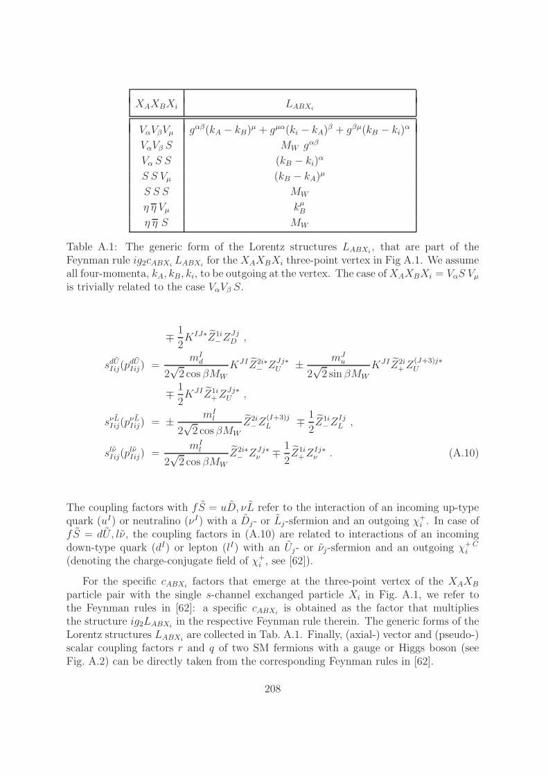
XAXBXi LABXi
VαVβVµ gαβ(kA − kB)µ + gµα(ki − kA)β + gβµ(kB − ki)αVαVβ S MW gαβ
Vα S S (kB − ki)αS S Vµ (kB − kA)µS S S MW
η η Vµ kµBη η S MW
Table A.1: The generic form of the Lorentz structures LABXi, that are part of the
Feynman rule ig2cABXiLABXi
for the XAXBXi three-point vertex in Fig A.1. We assumeall four-momenta, kA, kB, ki, to be outgoing at the vertex. The case ofXAXBXi = VαS Vµis trivially related to the case VαVβ S.
∓ 1
2KIJ∗Z1i
−ZJjD ,
sdUIij(pdUIij) =
mId
2√2 cos βMW
KJIZ2i∗− ZJj∗
U ± mJu
2√2 sin βMW
KJIZ2i+Z
(J+3)j∗U
∓ 1
2KJIZ1i
+ZJj∗U ,
sνLIij(pνLIij) = ± mI
l
2√2 cos βMW
Z2i−Z
(I+3)jL ∓ 1
2Z1i
−ZIjL ,
slνIij(plνIij) =
mIl
2√2 cos βMW
Z2i∗− ZJj∗
ν ∓ 1
2Z1i
+ZIj∗ν . (A.10)
The coupling factors with fS = uD, νL refer to the interaction of an incoming up-typequark (uI) or neutralino (νI) with a Dj- or Lj-sfermion and an outgoing χ+
i . In case offS = dU, lν, the coupling factors in (A.10) are related to interactions of an incomingdown-type quark (dI) or lepton (lI) with an Uj- or νj-sfermion and an outgoing χ+C
i
(denoting the charge-conjugate field of χ+i , see [62]).
For the specific cABXifactors that emerge at the three-point vertex of the XAXB
particle pair with the single s-channel exchanged particle Xi in Fig. A.1, we refer tothe Feynman rules in [62]: a specific cABXi
is obtained as the factor that multipliesthe structure ig2LABXi
in the respective Feynman rule therein. The generic forms of theLorentz structures LABXi
are collected in Tab. A.1. Finally, (axial-) vector and (pseudo-)scalar coupling factors r and q of two SM fermions with a gauge or Higgs boson (seeFig. A.2) can be directly taken from the corresponding Feynman rules in [62].
208
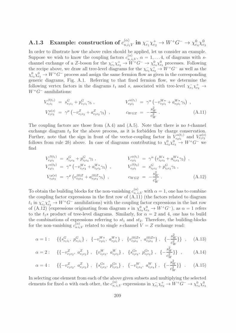
A.1.3 Example: construction of c(α)n,i1V
in χ−e1χ+e2 → W+G− → χ0
e4χ0e3
In order to illustrate how the above rules should be applied, let us consider an example.Suppose we wish to know the coupling factors c
(α)n, i1V
, α = 1, . . . 4, of diagrams with s-channel exchange of a Z-boson for the χ−
e1χ+e2→ W+G− → χ0
e4χ0e3
processes. Followingthe recipe above, we draw all tree-level diagrams for the χ−
e1χ+e2 → W+G− as well as the
χ0e4χ0e3→W+G− process and assign the same fermion flow as given in the corresponding
generic diagrams, Fig. A.1. Referring to that fixed fermion flow, we determine thefollowing vertex factors in the diagrams t1 and s, associated with tree-level χ−
e1χ+e2→
W+G− annihilations:
Vβ(t1)e1i1
= sGe1i1 + pGe1i1γ5 , Vα(t1)e2i1
= γα(−vW∗
e2i1 + aW∗e2i1γ5
),
V µ(s)e1e2
= γµ(−vZe1e2 + aZe1e2γ5
), cWGZ = −s
2W
c2W. (A.11)
The coupling factors are those from (A.4) and (A.5). Note that there is no t-channelexchange diagram t2 for the above process, as it is forbidden by charge conservation.Further, note that the sign in front of the vector-coupling factor in V
α(t1)e2i1
and Vµ(s)e1e2
follows from rule 2b) above. In case of diagrams contributing to χ0e4χ0e3→ W+G− we
find
Vβ(t1)e4i1
= sGi1e4 + pGi1e4γ5 , Vα(t1)e3i1
= γα(vW∗i1e3
+ aW∗i1e3
γ5),
Vα(t2)e4i1
= γα(−vW∗
i1e4+ aW∗
i1e4γ5), V
β(t2)e3i1
= sGi1e3 + pGi1e3γ5 ,
V µ(s)e4e3 = γµ
(v(0)Ze3e4 + a(0)Ze3e4 γ5
), cWGZ = −s
2W
c2W. (A.12)
To obtain the building blocks for the non-vanishing c(α)n, i1V
with α = 1, one has to combinethe coupling factor expressions in the first row of (A.11) (the factors related to diagramt1 in χ
−e1χ+e2→W+G− annihilations) with the coupling factor expressions in the last row
of (A.12) (expressions originating from diagram s in χ0e4χ0e3→ W+G−), as α = 1 refers
to the t1s product of tree-level diagrams. Similarly, for α = 2 and 4, one has to buildthe combinations of expressions referring to st1 and st2. Therefore, the building-blocksfor the non-vanishing c
(α)n i1V
related to single s-channel V = Z exchange read:
α = 1 : sGe1i1 , pGe1i1 , −vW∗
e2i1, aW∗
e2i1 , v(0)Z∗e3e4
, a(0)Z∗e3e4 , −s
2W
c2W , (A.13)
α = 2 : −vZe1e2, aZe1e2 , vWi1e3, a
Wi1e3 , sG∗
i1e4, pG∗
i1e4 , −s
2W
c2W , (A.14)
α = 4 : −vZe1e2, aZe1e2 , sG∗
i1e3, pG∗
i1e3 , −vWi1e4, a
Wi1e4 , −s
2W
c2W . (A.15)
In selecting one element from each of the above given subsets and multiplying the selectedelements for fixed α with each other, the c
(α)n, i1V
expressions in χ−e1χ
+e2 →W+G− → χ0
e4χ0e3
209
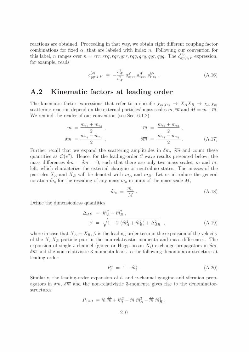
reactions are obtained. Proceeding in that way, we obtain eight different coupling factorcombinations for fixed α, that are labeled with index n. Following our convention forthis label, n ranges over n = rrr, rrq, rqr, qrr, rqq, qrq, qqr, qqq. The c
(2)qqr, i1V
expression,for example, reads
c(2)qqr, i1V
= −s2W
c2WaZe1e2 a
Wi1e3 s
G∗i1e4 . (A.16)
A.2 Kinematic factors at leading order
The kinematic factor expressions that refer to a specific χe1χe2 → XAXB → χe4χe3scattering reaction depend on the external particles’ mass scales m, m and M = m+m.We remind the reader of our convention (see Sec. 6.1.2)
m =me1 +me4
2, m =
me2 +me3
2,
δm =me4 −me1
2, δm =
me3 −me2
2. (A.17)
Further recall that we expand the scattering amplitudes in δm, δm and count thesequantities as O(v2). Hence, for the leading-order S-wave results presented below, themass differences δm = δm = 0, such that there are only two mass scales, m and m,left, which characterize the external chargino or neutralino states. The masses of theparticles XA and XB will be denoted with mA and mB. Let us introduce the generalnotation ma for the rescaling of any mass ma in units of the mass scale M ,
ma =ma
M. (A.18)
Define the dimensionless quantities
∆AB = m2A − m2
B ,
β =√1− 2 (m2
A + m2B) + ∆2
AB , (A.19)
where in case that XA = XB, β is the leading-order term in the expansion of the velocityof the XAXB particle pair in the non-relativistic momenta and mass differences. Theexpansion of single s-channel (gauge or Higgs boson Xi) exchange propagators in δm,δm and the non-relativistic 3-momenta leads to the following denominator-structure atleading order:
P si = 1− m2
i . (A.20)
Similarly, the leading-order expansion of t- and u-channel gaugino and sfermion prop-agators in δm, δm and the non-relativistic 3-momenta gives rise to the denominator-structures
Pi AB = m m+ m2i − m m2
A − m m2B ,
210
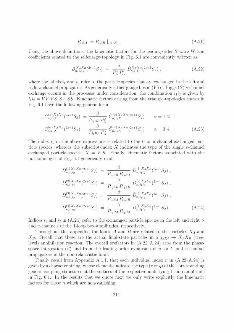
Pi BA = Pi AB |A↔B . (A.21)
Using the above definitions, the kinematic factors for the leading-order S-wave Wilsoncoefficients related to the selfenergy-topology in Fig. 6.1 are conveniently written as
BXAXB
n, i1i2(2s+1SJ) =
β
P si1P si2
BXAXB
n, i1i2(2s+1SJ) , (A.22)
where the labels i1 and i2 refer to the particle species that are exchanged in the left andright s-channel propagator. As generically either gauge boson (V ) or Higgs (S) s-channelexchange occurs in the processes under consideration, the combination i1i2 is given byi1i2 = V V, V S, SV, SS. Kinematic factors arising from the triangle-topologies shown inFig. 6.1 have the following generic form
C(α)XAXB
n, i1X(2s+1SJ) =
β
Pi1AB PsX
C(α)XAXB
n, i1X(2s+1SJ) α = 1, 2 ,
C(α)XAXB
n, i1X(2s+1SJ) =
β
Pi1BA PsX
C(α)XAXB
n, i1X(2s+1SJ) α = 3, 4 . (A.23)
The index i1 in the above expressions is related to the t- or u-channel exchanged par-ticle species, whereas the subscript-index X indicates the type of the single s-channelexchanged particle-species, X = V, S. Finally, kinematic factors associated with thebox-topologies of Fig. 6.1 generically read
D(1)XAXB
n, i1i2(2s+1SJ) =
β
Pi1AB Pi2BAD
(1)XAXB
n, i1i2(2s+1SJ) ,
D(2)XAXB
n, i1i2(2s+1SJ) =
β
Pi1AB Pi2ABD
(2)XAXB
n, i1i2(2s+1SJ) ,
D(3)XAXB
n, i1i2(2s+1SJ) =
β
Pi1BA Pi2ABD
(3)XAXB
n, i1i2(2s+1SJ) ,
D(4)XAXB
n, i1i2(2s+1SJ) =
β
Pi1BA Pi2BAD
(4)XAXB
n, i1i2(2s+1SJ) . (A.24)
Indices i1 and i2 in (A.24) refer to the exchanged particle species in the left and right t-and u-channels of the 1-loop box-amplitudes, respectively.
Throughout this appendix, the labels A and B are related to the particles XA andXB. Recall that these are the actual final-state particles in a χiχj → XAXB (tree-level) annihilation reaction. The overall prefactors in (A.22–A.24) arise from the phase-space integration (β) and from the leading-order expansion of s- or t- and u-channelpropagators in the non-relativistic limit.
Finally recall from Appendix A.1.1, that each individual index n in (A.22–A.24) isgiven by a character string, whose elements indicate the type (r or q) of the correspondinggeneric coupling structures at the vertices of the respective underlying 1-loop amplitudein Fig. 6.1. In the results that we quote next we only write explicitly the kinematicfactors for those n which are non-vanishing.
211

A.2.1 Kinematic factors for XAXB = V V
The kinematic factors BV Vn, i1i2
in case of 1S0 partial-wave reactions are given by
BV Vqq, V V (
1S0) = − β2
2+ 3 ∆2
AB , (A.25)
BV Vqq, V S(
1S0) = BV Vqq, SV (
1S0) = 3 mW∆AB , (A.26)
BV Vqq, SS(
1S0) = 4 m2W . (A.27)
In case of 3S1 partial-wave reactions we have
BV Vrr, V V (
3S1) = − 9
2+
4
3β2 − 1
2∆2AB . (A.28)
Only the kinematic factors BV Vn, i1i2 given explicitly in (A.25–A.28) with n = rr, qq are
non-vanishing. In case of XAXB = V V , the kinematic factors for the triangle- and box-diagram topologies α = 3, 4 are related to the corresponding expressions for diagram-topologies α = 1, 2 (see Fig. 6.1). The relations read
C(3) V Vn, i1V
(2s+1SJ) = − C(1) V Vn, i1V
(2s+1SJ) |A↔B ,
C(4) V Vn, i1V
(2s+1SJ) = − C(2) V Vn, i1V
(2s+1SJ) |A↔B ,
C(3) V Vn, i1S
(2s+1SJ) = C(1) V Vn, i1S
(2s+1SJ) |A↔B ,
C(4) V Vn, i1S
(2s+1SJ) = C(2) V Vn, i1S
(2s+1SJ) |A↔B ,
D(3) V Vn, i1i2
(2s+1SJ) = D(1) V Vn, i1i2
(2s+1SJ) |A↔B ,
D(4) V Vn, i1i2
(2s+1SJ) = D(2) V Vn, i1i2
(2s+1SJ) |A↔B . (A.29)
The minus sign in the relation for the triangle coefficients C(α) V Vn, i1V
in (A.29) arises frominterchanging the two gauge bosons XA and XB at the internal three-gauge boson vertex.The expressions C
(α) V Vn, i1V
for diagram-topologies α = 1, 2, that refer to leading-order 1S0
partial waves read
C(1) V Vrqq, i1V
(1S0) =β2
2− 3
2(m− m)∆AB −
3
2∆2AB + 3 mi1∆AB , (A.30)
C(2) V Vqqr, i1V
(1S0) = C(1) V Vrqq, i1V
(1S0) . (A.31)
In case of C(α)V Vn, i1V
expressions related to 3S1 partial waves and diagram-topologies α = 1, 2we find
C(α) V Vrrr, i1V
(3S1) = − 5
6β2 + (m− m)
∆AB
2+
∆2AB
2+ 3 mi1 . (A.32)
We deduce the following expressions for C(α) V Vn, i1S
coefficients and diagram topologies α =1, 2:
C(1) V Vrqq, i1S
(1S0) = C(2) V Vqqr, i1S
(1S0) = −mW (m− m+∆AB) + 4 mW mi1 . (A.33)
212
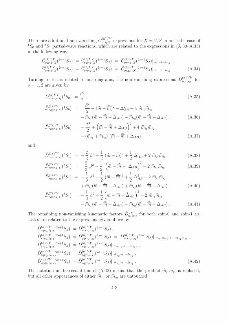
There are additional non-vanishing C(α)V Vn, i1X
expressions for X = V, S in both the case of1S0 and 3S1 partial-wave reactions, which are related to the expressions in (A.30–A.33)in the following way:
C(1) V Vqqr, i1X
(2s+1SJ) = C(2) V Vrqq, i1X
(2s+1SJ) = C(1) V Vrrr, i1X
(2s+1SJ)|mi1→−mi1
,
C(1) V Vqrq, i1X
(2s+1SJ) = C(2) V Vqrq, i1X
(2s+1SJ) = C(1) V Vrqq, i1X
(2s+1SJ)|mi1→−mi1
. (A.34)
Turning to terms related to box-diagrams, the non-vanishing expressions D(α)V Vn, i1i2
forα = 1, 2 are given by
D(α)V Vrrrr, i1i2
(1S0) =β2
2, (A.35)
D(1) V Vrqqr, i1i2
(1S0) =β2
2+ (m− m)2 −∆2
AB + 4 mi1mi2
− mi1(m− m−∆AB)− mi2(m− m+∆AB) , (A.36)
D(2), V Vrqqr, i1i2
(1S0) = − β2
2+(m− m+∆AB
)2+ 4 mi1mi2
− (mi1 + mi2) (m− m+∆AB) , (A.37)
and
D(1) V Vrrrr, i1i2
(3S1) = − 2
3β2 − 1
2(m− m)2 +
1
2∆2AB + 2 mi1mi2 , (A.38)
D(2) V Vrrrr, i1i2
(3S1) =2
3β2 − 1
2
(m− m+ ∆AB
)2− 2 mi1mi2 , (A.39)
D(1) V Vrqqr, i1i2
(3S1) = − 1
3β2 − 1
2(m− m)2 +
1
2∆2AB − 2 mi1mi2
+ mi1(m− m−∆AB) + mi2(m− m+∆AB) , (A.40)
D(2) V Vrqqr, i1i2
(3S1) = − 1
3β2 +
1
2
(m−m+ ∆AB
)2+ 2 mi1mi2
− mi1(m− m+∆AB)− mi2(m− m+∆AB) . (A.41)
The remaining non-vanishing kinematic factors DV Vn, i1i2
for both spin-0 and spin-1 χχstates are related to the expressions given above by
D(α) V Vqqqq, i1i2
(2s+1SJ) = D(α) V Vrrrr, i1i2
(2s+1SJ) ,
D(α)V Vrrqq, i1i2
(2s+1SJ) = D(α) V Vqqrr, i1i2
(2s+1SJ) = D(α) V Vrrrr, i1i2
(2s+1SJ)| m i1m i2
→ −m i1m i2
,
D(α)V Vqrrq, i1i2
(2s+1SJ) = D(α) V Vrqqr, i1i2
(2s+1SJ)| m i1,2→ −m i1,2
,
D(α)V Vrqrq, i1i2
(2s+1SJ) = D(α) V Vrqqr, i1i2
(2s+1SJ)| m i2→ −m i2
,
D(α)V Vqrqr, i1i2
(2s+1SJ) = D(α) V Vrqqr, i1i2
(2s+1SJ)| m i1→ −m i1
. (A.42)
The notation in the second line of (A.42) means that the product mi1mi2 is replaced,but all other appearances of either mi1 or mi2 are untouched.
213
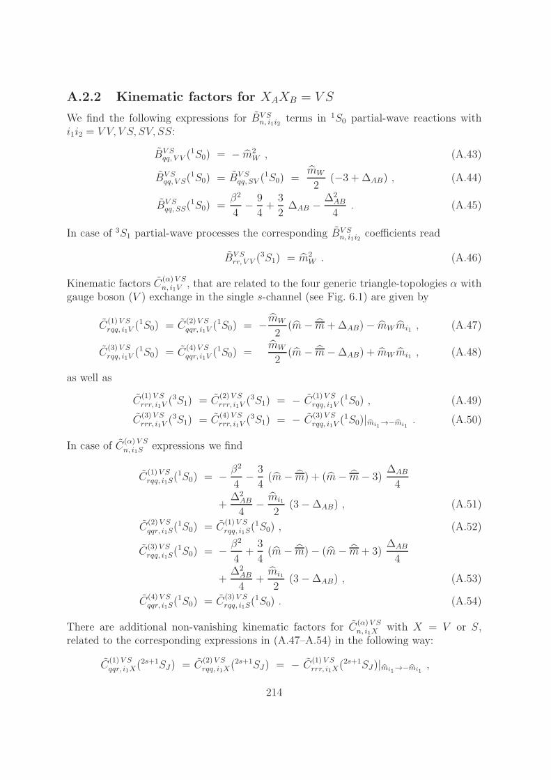
A.2.2 Kinematic factors for XAXB = V S
We find the following expressions for BV Sn, i1i2
terms in 1S0 partial-wave reactions withi1i2 = V V, V S, SV, SS:
BV Sqq, V V (
1S0) = − m2W , (A.43)
BV Sqq, V S(
1S0) = BV Sqq, SV (
1S0) =mW
2(−3 + ∆AB) , (A.44)
BV Sqq, SS(
1S0) =β2
4− 9
4+
3
2∆AB −
∆2AB
4. (A.45)
In case of 3S1 partial-wave processes the corresponding BV Sn, i1i2
coefficients read
BV Srr, V V (
3S1) = m2W . (A.46)
Kinematic factors C(α) V Sn, i1V
, that are related to the four generic triangle-topologies α withgauge boson (V ) exchange in the single s-channel (see Fig. 6.1) are given by
C(1) V Srqq, i1V
(1S0) = C(2)V Sqqr, i1V
(1S0) = −mW
2(m− m+∆AB)− mW mi1 , (A.47)
C(3) V Srqq, i1V
(1S0) = C(4)V Sqqr, i1V
(1S0) =mW
2(m− m−∆AB) + mW mi1 , (A.48)
as well as
C(1) V Srrr, i1V
(3S1) = C(2) V Srrr, i1V
(3S1) = − C(1) V Srqq, i1V
(1S0) , (A.49)
C(3) V Srrr, i1V
(3S1) = C(4) V Srrr, i1V
(3S1) = − C(3) V Srqq, i1V
(1S0)|mi1→−mi1
. (A.50)
In case of C(α) V Sn, i1S
expressions we find
C(1) V Srqq, i1S
(1S0) = − β2
4− 3
4(m− m) + (m− m− 3)
∆AB
4
+∆2AB
4− mi1
2(3−∆AB) , (A.51)
C(2) V Sqqr, i1S
(1S0) = C(1) V Srqq, i1S
(1S0) , (A.52)
C(3) V Srqq, i1S
(1S0) = − β2
4+
3
4(m− m)− (m− m+ 3)
∆AB
4
+∆2AB
4+mi1
2(3−∆AB) , (A.53)
C(4) V Sqqr, i1S
(1S0) = C(3) V Srqq, i1S
(1S0) . (A.54)
There are additional non-vanishing kinematic factors for C(α) V Sn, i1X
with X = V or S,related to the corresponding expressions in (A.47–A.54) in the following way:
C(1) V Sqqr, i1X
(2s+1SJ) = C(2) V Srqq, i1X
(2s+1SJ) = − C(1) V Srrr, i1X
(2s+1SJ)|mi1→−mi1
,
214
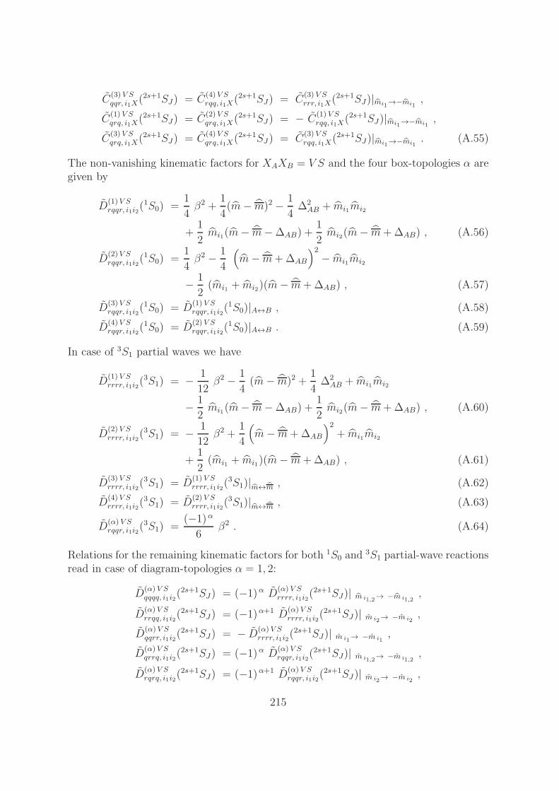
C(3) V Sqqr, i1X
(2s+1SJ) = C(4) V Srqq, i1X
(2s+1SJ) = C(3) V Srrr, i1X
(2s+1SJ)|mi1→−mi1
,
C(1) V Sqrq, i1X
(2s+1SJ) = C(2) V Sqrq, i1X
(2s+1SJ) = − C(1) V Srqq, i1X
(2s+1SJ)|mi1→−mi1
,
C(3) V Sqrq, i1X
(2s+1SJ) = C(4) V Sqrq, i1X
(2s+1SJ) = C(3) V Srqq, i1X
(2s+1SJ)|mi1→−mi1
. (A.55)
The non-vanishing kinematic factors for XAXB = V S and the four box-topologies α aregiven by
D(1)V Srqqr, i1i2
(1S0) =1
4β2 +
1
4(m− m)2 − 1
4∆2AB + mi1mi2
+1
2mi1(m− m−∆AB) +
1
2mi2(m− m+∆AB) , (A.56)
D(2)V Srqqr, i1i2
(1S0) =1
4β2 − 1
4
(m− m+∆AB
)2− mi1mi2
− 1
2(mi1 + mi2)(m− m+∆AB) , (A.57)
D(3)V Srqqr, i1i2
(1S0) = D(1) V Srqqr, i1i2
(1S0)|A↔B , (A.58)
D(4)V Srqqr, i1i2
(1S0) = D(2) V Srqqr, i1i2
(1S0)|A↔B . (A.59)
In case of 3S1 partial waves we have
D(1) V Srrrr, i1i2
(3S1) = − 1
12β2 − 1
4(m− m)2 +
1
4∆2AB + mi1mi2
− 1
2mi1(m− m−∆AB) +
1
2mi2(m− m+∆AB) , (A.60)
D(2) V Srrrr, i1i2
(3S1) = − 1
12β2 +
1
4
(m− m+∆AB
)2+ mi1mi2
+1
2(mi1 + mi1)(m− m+∆AB) , (A.61)
D(3) V Srrrr, i1i2
(3S1) = D(1) V Srrrr, i1i2
(3S1)|m↔m , (A.62)
D(4) V Srrrr, i1i2
(3S1) = D(2) V Srrrr, i1i2
(3S1)|m↔m , (A.63)
D(α) V Srqqr, i1i2
(3S1) =(−1)α
6β2 . (A.64)
Relations for the remaining kinematic factors for both 1S0 and3S1 partial-wave reactions
read in case of diagram-topologies α = 1, 2:
D(α) V Sqqqq, i1i2
(2s+1SJ) = (−1)α D(α) V Srrrr, i1i2
(2s+1SJ)| m i1,2→ −m i1,2
,
D(α) V Srrqq, i1i2
(2s+1SJ) = (−1)α+1 D(α) V Srrrr, i1i2
(2s+1SJ)| m i2→ −m i2
,
D(α) V Sqqrr, i1i2
(2s+1SJ) = − D(α) V Srrrr, i1i2
(2s+1SJ)| m i1→ −m i1
,
D(α) V Sqrrq, i1i2
(2s+1SJ) = (−1)α D(α) V Srqqr, i1i2
(2s+1SJ)| m i1,2→ −m i1,2
,
D(α) V Srqrq, i1i2
(2s+1SJ) = (−1)α+1 D(α) V Srqqr, i1i2
(2s+1SJ)| m i2→ −m i2
,
215
D(α) V Sqrqr, i1i2
(2s+1SJ) = − D(α) V Srqqr, i1i2
(2s+1SJ)| m i1→ −m i1
. (A.65)
The corresponding relations for diagram-topologies α = 3, 4 are given by
D(α) V Sqqqq, i1i2
(2s+1SJ) = (−1)α D(α) V Srrrr, i1i2
(2s+1SJ)| m i1,2→ −m i1,2
,
D(α) V Srrqq, i1i2
(2s+1SJ) = (−1)α D(α) V Srrrr, i1i2
(2s+1SJ)| m i2→ −m i2
,
D(α) V Sqqrr, i1i2
(2s+1SJ) = D(α) V Srrrr, i1i2
(2s+1SJ)| m i1→ −m i1
,
D(α) V Sqrrq, i1i2
(2s+1SJ) = (−1)α D(α) V Srqqr, i1i2
(2s+1SJ)| m i1,2→ −m i1,2
,
D(α) V Srqrq, i1i2
(2s+1SJ) = (−1)α D(α) V Srqqr, i1i2
(2s+1SJ)| m i2→ −m i2
,
D(α) V Sqrqr, i1i2
(2s+1SJ) = D(α) V Srqqr, i1i2
(2s+1SJ)| m i1→ −m i1
. (A.66)
A.2.3 Kinematic factors for XAXB = SS
The non-vanishing BSSn, i1i2
terms with i1i2 = V V, V S, SV, V V read
BSSqq, V V (
1S0) = ∆2AB , (A.67)
BSSqq, V S(
1S0) = BSSqq, SV (
1S0) = − mW∆AB , (A.68)
BSSqq, SS(
1S0) = m2W , (A.69)
and in case of 3S1 reactions
BSSrr, V V (
3S1) =β2
3. (A.70)
As in the case of XAXB = V V , the kinematic factors for XAXB = SS and diagramtopologies α = 3, 4 are related to the corresponding expressions that arise from diagram-topologies α = 1, 2. This applies to both triangle- and box-topologies (see Fig. 6.1):
C(3)SSn, i1V
(2s+1SJ) = − C(1)SSn, i1V
(2s+1SJ) |A↔B ,
C(4)SSn, i1V
(2s+1SJ) = − C(2)SSn, i1V
(2s+1SJ) |A↔B ,
C(3)SSn, i1S
(2s+1SJ) = C(1)SSn, i1S
(2s+1SJ) |A↔B ,
C(4)SSn, i1S
(2s+1SJ) = C(2)SSn, i1S
(2s+1SJ) |A↔B ,
D(3)SSn, i1i2
(2s+1SJ) = D(1)SSn, i1i2
(2s+1SJ) |A↔B ,
D(4)SSn, i1i2
(2s+1SJ) = D(2)SSn, i1i2
(2s+1SJ) |A↔B . (A.71)
In case of expressions C(α)SSn, i1V
for diagram-topologies α = 1, 2 we find
C(1)SSrqq, i1V
(1S0) = C(2)SSqqr, i1V
(1S0) =∆AB
2(m− m+∆AB) + mi1∆AB , (A.72)
C(1)SSrrr, i1V
(3S1) = C(2)SSrrr, i1V
(3S1) = − β2
6. (A.73)
216
The C(α)SSn, i1S
expressions with α = 1, 2 are given by
C(1)SSrqq, i1S
(1S0) = C(2)SSqqr, i1S
(1S0) = −mW
2(m− m+∆AB)− mW mi1 . (A.74)
All other non-vanishing expressions for C(α)SSn, i1X
with X = V, S and α = 1, 2 can be relatedto the terms in (A.72–A.74) in the following way:
C(1)SSqqr, i1X
(2s+1SJ) = C(2)SSrqq, i1X
(2s+1SJ) = − C(1)SSrrr, i1X
(2s+1SJ)|mi1→−mi1
,
C(1)SSqrq, i1X
(2s+1SJ) = C(2)SSqrq, i1X
(2s+1SJ) = − C(1)SSrqq, i1X
(2s+1SJ)|mi1→−mi1
. (A.75)
The expressions D(α)SSn, i1i2
for diagram-topologies α = 1, 2 and 1S0 partial waves read
D(1)SSrqqr, i1i2
(1S0) =1
4(m− m)2 − ∆2
AB
4+ mi1mi2
+mi1
2(m− m−∆AB) +
mi2
2(m− m+∆AB) , (A.76)
D(2)SSrqqr, i1i2
(1S0) =1
4
(m− m+∆AB
)2+ mi1mi2
+1
2(mi1 + mi2)(m− m+∆AB) . (A.77)
In case of a 3S1 partial-wave configuration we find
D(α)SSrrrr, i1i2
(3S1) = (−1)α β2
12. (A.78)
The remaining non-vanishing kinematic factors related to both 1S0 and3S1 partial-wave
reactions read
D(α)SSqqqq, i1i2
(2s+1SJ) = D(α)SSrrrr, i1i2
(2s+1SJ) ,
D(α)SSrrqq, i1i2
(2s+1SJ) = D(α)SSqqrr, i1i2
(2s+1SJ) = −D(α)SSrrrr, i1i2
(2s+1SJ) ,
D(α)SSqrrq, i1i2
(2s+1SJ) = D(α)SSrqqr, i1i2
(2s+1SJ)| m i1,2→ −m i1,2
,
D(α)SSrqrq, i1i2
(2s+1SJ) = − D(α)SSrqqr, i1i2
(2s+1SJ)| m i2→ −m i2
,
D(α)SSqrqr, i1i2
(2s+1SJ) = − D(α)SSrqqr, i1i2
(2s+1SJ)| m i1→ −m i1
. (A.79)
A.2.4 Kinematic factors for XAXB = ff
The non-vanishing Bffn, i1i2
terms with i1i2 = V V, V S, SV, SS are given by
Bffqqqq, V V (
1S0) = 1− β2 + 4 mAmB −∆2AB , (A.80)
Bffqqqq, V S(
1S0) = Bffqqqq, SV (
1S0) = 2(mA + mB − (mA − mB)∆AB
), (A.81)
217
Bffqqqq, SS(
1S0) = 1 + β2 + 4 mAmB −∆2AB , (A.82)
and in case of 3S1 partial-wave reactions
Bffrrrr, V V (
3S1) = 1 +β2
3+ 4 mAmB −∆2
AB . (A.83)
There are additional non-vanishing terms Bffn, i1i2
related to the expressions in (A.80–A.83). In case of i1i2 = V V, SS, the corresponding relations read
Bffrqqr, i1i2
(2s+1SJ) = Bffrrrr, i1i2
(2s+1SJ)|mAmB→−mAmB, (A.84)
Bffqrrq, i1i2
(2s+1SJ) = Bffqqqq, i1i2
(2s+1SJ)|mAmB→−mAmB, (A.85)
and our notation implies, that the product mAmB has to be replaced, but all otheroccurrences of mA or mB are untouched. Similarly, in case of i1i2 = V S, SV , theadditional non-vanishing Bff
n, i1i2terms are given by
Bffrqqr, i1i2
(2s+1SJ) = − Bffrrrr, i1i2
(2s+1SJ)|mA→−mA, (A.86)
Bffqrrq, i1i2
(2s+1SJ) = − Bffqqqq, i1i2
(2s+1SJ)|mA→−mA. (A.87)
The relations among kinematic factors for diagram topologies α = 3, 4 and diagram-topologies α = 1, 2 in both the cases of box- and triangle-topologies are given by (X =V, S)
C(3) ffn, i1X
(2s+1SJ) = C(1) ffn, i1X
(2s+1SJ) |A↔B , (A.88)
C(4) ffn, i1X
(2s+1SJ) = C(2) ffn, i1X
(2s+1SJ) |A↔B , (A.89)
D(3) ffn, i1i2
(2s+1SJ) = D(1) ffn, i1i2
(2s+1SJ) |A↔B , (A.90)
D(4) ffn, i1i2
(2s+1SJ) = D(2) ffn, i1i2
(2s+1SJ) |A↔B , (A.91)
compare to the generic diagrams in Fig. 6.1. The structures C(α) ffn, i1V
for topologies α = 1, 2are given by
C(α) ffqqqq, i1V
(1S0) =β2
4− 1
4(1− 2 mA)(1− 2 mB)
− (mA − mB)∆AB
2− ∆2
AB
4, (A.92)
and in case of 3S1 partial-wave reactions the respective expressions read
C(α) ffrrrr, i1V
(3S1) = − β2
12− 1
4(1 + 2 mA)(1 + 2 mB)
+ (mA − mB)∆AB
2+
∆2AB
4. (A.93)
218

The relations of the additional non-vanishing C(α) ffn, i1V
expressions to the respective termsin (A.92–A.93) read
C(1) ffqqrr, i1V
(2s+1SJ) = C(2) ffrrqq, i1V
(2s+1SJ) = − C(1) ffrrrr, i1V
(2s+1SJ)|mA,B→−mA,B,
C(α) ffrqqr, i1V
(2s+1SJ) = C(α) ffrrrr, i1V
(2s+1SJ)|mA→−mA,
C(1) ffqrqr, i1V
(2s+1SJ) = C(2) ffrqrq, i1V
(2s+1SJ) = − C(1) ffrrrr, i1V
(2s+1SJ)|mB→−mB,
C(1) ffrqrq, i1V
(2s+1SJ) = C(2) ffqrqr, i1V
(2s+1SJ) = − C(α) ffqqqq, i1V
(2s+1SJ)|mB→−mB,
C(α) ffqrrq, i1V
(2s+1SJ) = C(α) ffqqqq, i1V
(2s+1SJ)|mA→−mA,
C(1) ffrrqq, i1V
(2s+1SJ) = C(2) ffqqrr, i1V
(2s+1SJ) = − C(α) ffqqqq, i1V
(2s+1SJ)|mA,B→−mA,B. (A.94)
The terms C(α) ffn, i1S
for α = 1, 2 read
C(α) ffqqqq, i1S
(1S0) =β2
4+
1
4(1− 2 mA)(1− 2 mB)
+ (mA − mB)∆AB
2− ∆2
AB
4, (A.95)
and all remaining non-vanishing C(α) ffn, i1S
terms are obtained from (A.95) in the followingway:
C(1) ffrqrq, i1S
(2s+1SJ) = C(2) ffqrqr, i1S
(2s+1SJ) = C(α) ffqqqq, i1S
(2s+1SJ)|mB→−mB,
C(α) ffqrrq, i1S
(2s+1SJ) = C(α) ffqqqq, i1S
(2s+1SJ)|mA→−mA,
C(1) ffrrqq, i1S
(2s+1SJ) = C(2) ffqqrr, i1S
(2s+1SJ) = C(α) ffqqqq, i1S
(2s+1SJ)|mA,B→−mA,B. (A.96)
In case of box-diagram topologies α = 1, 2, we find the following D(α) ffn, i1i2
structures forthe 1S0 partial waves:
D(α) ffrrrr, i1i2
(1S0) =1
8(1 + 2 mB −∆AB)(1 + 2 mA +∆AB) , (A.97)
D(α) ffrrqq, i1i2
(1S0) =β2
8− 1
2mAmB . (A.98)
For 3S1 partial-wave configurations we have
D(α) ffrrrr i1i2
(3S1) = (−1)α D(α) ffrrrr, i1i2
(1S0) , (A.99)
D(α) ffrrqq, i1i2
(3S1) = (−1)α+1
(β2
24+
1
2mAmB
). (A.100)
Relations for the remaining non-vanishing kinematic factors related to both 1S0 and3S1
partial-wave processes read in case of diagram topology α = 1
D(1) ffqqqq, i1i2
(2s+1SJ) = D(1) ffrrrr, i1i2
(2s+1SJ)| mA,B→ −mA,B,
219
D(1) ffqqrr, i1i2
(2s+1SJ) = D(1) ffrrqq, i1i2
(2s+1SJ) ,
D(1) ffrqqr, i1i2
(2s+1SJ) = D(1) ffqrrq, i1i2
(2s+1SJ) = D(1) ffrrqq, i1i2
(2s+1SJ)| mAmB→ −mAmB,
D(1) ffrqrq, i1i2
(2s+1SJ) = D(1) ffrrrr, i1i2
(2s+1SJ)| mA→ −mA,
D(1) ffqrqr, i1i2
(2s+1SJ) = D(1) ffrrrr, i1i2
(2s+1SJ)| mB→ −mB. (A.101)
In case of diagram topology α = 2, the corresponding relations are given by
D(2) ffqqqq, i1i2
(2s+1SJ) = D(2) ffrrrr, i1i2
(2s+1SJ)| mA,B→ −mA,B,
D(2) ffqqrr, i1i2
(2s+1SJ) = D(2) ffrrqq, i1i2
(2s+1SJ) ,
D(2) ffrqqr, i1i2
(2s+1SJ) = D(2) ffrrrr, i1i2
(2s+1SJ)| mA→ −mA,
D(2) ffqrrq, i1i2
(2s+1SJ) = D(2) ffrrrr, i1i2
(2s+1SJ)| mB→ −mB,
D(2) ffrqrq, i1i2
(2s+1SJ) = D(2) ffqrqr, i1i2
(2s+1SJ) = D(2) ffrrqq, i1i2
(2s+1SJ)| mAmB→ −mAmB. (A.102)
A.2.5 Kinematic factors for XAXB = ηη
In case of XAXB = ηη one cannot directly construct the coupling factors bn i1i2 usingthe recipe given in Sec. A.1.1, which is based on considering the χe1χe2 → XAXB andχe4χe3 → XAXB tree-level annihilation amplitudes. In order to obtain the couplingfactor expressions bn i1i2, that correspond to the kinematic factors presented below, oneshould proceed as follows: First extract the (axial-) vector and (pseudo-) scalar couplingfactors associated with the interaction of the χe1χe2 or χe4χe3 pair and the s-channelexchanged particle species. This is done following the steps 1. and 2. in the recipegiven in Sec. A.1.1. Next, complex-conjugate the couplings related to the χe4χe3 particlepair. In order to determine the couplings to the ghosts, consider the 1-loop amplitudeχe1χe2 → ηη → χe4χe3, similar to the selfenergy-amplitude in Fig. 6.1. Assign a ghostflow to the lower line of the 1-loop amplitude (labeled with XA in Fig. 6.1), that flowsfrom left to right. Consequently there is a ghost flow from right to left on the upperline, which is labeled with XB. Assume that the coupling factors at each of the twoghost vertices are generically of the form ig2cABXi
LABXi, where the Lorentz structures
LABXiare defined in Tab. A.1. Determine the expressions that replace the generic cABXi
factors for the specific process under consideration. Now build all possible combinationsof two-coupling factor products from the set of the neutralino/chargino couplings to thes-channel exchanged particles (including factors of −1 in front of vector couplings) inthe χe1χe2 → ηη → χe4χe3 reaction, and multiply them by the cABXi1
and cABXi2factors.
The convention for the naming of the resulting coupling factor expressions bn, i1i2 withsubscripts n = rr, qq is the same as in the cases XAXB = V V, V S, SS, see Sec. A.1.1.The coupling factors bn, i1i2 derived in this way correspond to the kinematic factors givenbelow. Note that the mass parameter mA in the expressions below refers to the mass ofthe ghost flowing in the lower line, and mB to the mass of the ghost in the upper line.
220

The non-vanishing Bηηn, i1i2
terms with i1i2 = V V, V S, SV, SS read
Bηηqq, V V (
1S0) =1
4(1−∆2
AB) , (A.103)
Bηηqq, V S(
1S0) = − mW
2(1 + ∆AB) , (A.104)
Bηηqq, SV (
1S0) =mW
2(1−∆AB) , (A.105)
Bηηqq, SS(
1S0) = − m2W . (A.106)
Similarly,
Bηηrr, V V (
3S1) = − β2
12. (A.107)
A.3 Kinematic factors at O(v2)Throughout this section we rely on the same definitions and conventions for the massesm,m, the mass differences δm, δm and the mass ratio ma as established in (A.17) and(A.18) in Sec. A.2. Further, the same definitions for the parameters ∆AB and β, (A.19),are used and parameters P s
i and Pi AB, Pi BA are defined through (A.20) and (A.21).Regarding the presentation of results for the kinematic factors related to dimension-
8 operators in δLann, it is however convenient to use a notation where factors of theleading-order propagator and (m m), as well as the factor β arising from the phase-space integration are pulled out. This implies that the relations (A.22) and (A.23),introduced to clearly arrange the presentation of leading-order S-wave kinematic factorresults corresponding to selfenergy- and triangle-diagrams, differ from the correspondingrelations, that we now introduce for the kinematic factors related to the dimension-8operators: For the kinematic factors related to dimension-8 four-fermion operators, thatderive from the selfenergy topology we define
BXAXB
n, i1i2(2s+1LJ ) =
β
(m m)2 P si1P si2
BXAXB
n, i1i2(2s+1LJ ) , (A.108)
where the labels i1 and i2 refer to the particle species that are exchanged in the left andright s-channel propagator of the selfenergy diagram. As before, the combination i1i2 isgiven by i1i2 = V V, V S, SV, SS. Note that compared to (A.22) there is an additionalfactor (m m)2 in the denominator of (A.108). Likewise, we rewrite the kinematic factorsof dimension-8 Wilson coefficients arising from the triangle-topologies as
C(α)XAXB
n, i1X(2s+1LJ) =
β
m m Pi1AB PsX
C(α)XAXB
n, i1X(2s+1LJ) α = 1, 2 ,
C(α)XAXB
n, i1X(2s+1LJ) =
β
m m Pi1BA PsX
C(α)XAXB
n, i1X(2s+1LJ) α = 3, 4 , (A.109)
221
such that compared to (A.23) there appears an additional factor m m in the denominator.As in (A.23), the index i1 is related to the t- or u-channel exchanged particle species,and the subscript-index X indicates the type of exchanged particle (X = V, S) in the s-channel. Finally, the kinematic factors associated with the box topologies are written inthe same form as the correspondent expressions related to leading dimension-6 operators(A.24):
D(1)XAXB
n, i1i2(2s+1LJ ) =
β
Pi1AB Pi2BAD
(1)XAXB
n, i1i2(2s+1LJ) ,
D(2)XAXB
n, i1i2(2s+1LJ ) =
β
Pi1AB Pi2ABD
(2)XAXB
n, i1i2(2s+1LJ) ,
D(3)XAXB
n, i1i2(2s+1LJ ) =
β
Pi1BA Pi2ABD
(3)XAXB
n, i1i2(2s+1LJ) ,
D(4)XAXB
n, i1i2(2s+1LJ ) =
β
Pi1BA Pi2BAD
(4)XAXB
n, i1i2(2s+1LJ) . (A.110)
In (A.110) the indices i1 and i2 refer to the exchanged particle species in the left andright t- and u-channels of the 1-loop box amplitudes, respectively.
The conventions for the label n are the same as in Sec. A.2 (see Sec. A.1.1 for thecorresponding definitions). Again we quote in the following only those kinematic factorswith a given label n, that are non-vanishing.
A.3.1 P -wave kinematic factors for XAXB = V V
The only non-vanishing kinematic factor BV Vn, i1i2
in case of 1P1 partial-wave reactions isgiven by
BV Vqq, V V (
1P1) =∆2m
24
(8 β2 − 3 ∆2
AB − 27), (A.111)
while for the combined 3PJ waves the non-vanishing kinematic factors read
BV Vrr, V V (
3PJ ) = − ∆2m
8
(β2 − 6 ∆2
AB
), (A.112)
BV Vqq, V V (
3PJ ) =1
12
(8 β2 − 3 ∆2
AB − 27), (A.113)
BV Vrr, V S(
3PJ ) = BV Vrr, SV (
3PJ ) = −34mW ∆m ∆AB , (A.114)
BV Vrr, SS(
3PJ ) = m2W . (A.115)
As regards kinematic factors related to triangle- and box-topologies in the case XAXB =V V , the relations (A.29) among the α = 1(2) and α = 3(4) kinematic factors are ful-filled for any 2s+1LJ configuration (in particular also for the kinematic factors associatedwith the absorptive part of the next-to-next-to-leading order S-wave Wilson coefficients,g(2s+1Ss) and hi(
2s+1Ss)). By virtue of the relations (A.29), we therefore only need to
222
give here the kinematic factors for diagram-topologies α = 1, 2 for both the cases oftriangle and box diagram kinematic factors. Starting with the expressions C
(α) V Vn, i1V
for1P1 partial waves we have
C(1) V Vrqq, i1V
(1P1) =3 mi1
4 m m∆m +
β2 ∆m
12 Pi1AB(∆m − 6 mi1 + 2 ∆AB)
+∆m
24 m m
(6 ∆2
m ∆AB −∆m(5 β2 − 3 ∆2
AB)− 3 ∆AB
), (A.116)
C(2) V Vqqr, i1V
(1P1) = C(1) V Vrqq, i1V
(1P1) , (A.117)
whereas for the combined 3PJ quantum numbers we find
C(1) V Vrrr, i1V
(3PJ ) =3 mi1
4 m m∆m ∆AB +
β2 ∆m
12 Pi1AB(∆m + 2 ∆AB)
− ∆m
8 m m
(2 ∆2
m∆AB −∆m (β2 − 3 ∆2AB) + ∆AB
), (A.118)
C(2) V Vrrr, i1V
(3PJ ) = C(1) V Vrrr, i1V
(3PJ ) , (A.119)
C(1)V Vrqq, i1V
(3PJ ) =3 mi1
2 m m∆m −
β2
2 Pi1AB
− 1
12 m m
(5 β2 − 9 + 9 ∆2
m − 3 ∆AB (∆m +∆AB)), (A.120)
C(2) V Vqqr, i1V
(3PJ ) = C(1) V Vrqq, i1V
(3PJ ) . (A.121)
The coefficients C(α) V Vn, i1S
(1P1), corresponding to triangles with a Higgs particle exchangedin the s-channel, vanish for all n. The corresponding expressions related to 3PJ reactionsread for diagram topologies α = 1, 2
C(α) V Vrrr, i1S
(3PJ ) = − mW mi1
m m− β2 mW
6 Pi1AB+
mW
4 m m(∆m ∆AB + 1) . (A.122)
All the remaining non-vanishing kinematic factors C(α) V Vn, i1X
associated with 1P1 and 3PJscattering reactions with both X = V, S are related to the above expressions by
C(1) V Vqqr, i1X
(2s+1PJ) = C(2) V Vrqq, i1X
(2s+1PJ) = C(1) V Vrrr, i1X
(2s+1PJ)|mi1→−mi1
,
C(1) V Vqrq, i1X
(2s+1PJ) = C(2) V Vqrq, i1X
(2s+1PJ) = C(1) V Vrqq, i1X
(2s+1PJ)|mi1→−mi1
, (A.123)
where these relations hold in particular in case of separate 3PJ , J = 0, 1, 2, partial-waveconfigurations and hence trivially for the combined 3PJ waves. Finally, the terms relatedto box diagrams give rise to the following non-vanishing coefficients
D(1)V Vrrrr,i1i2
(1P1)
= − mi1mi2
4 (m m)2− mi1
4 (m m)2(∆m ∆AB − 1)
223
− 1
48 (m m)2
(∆2m (2 β2 − 3 ∆2
AB) + 3)− β4
12 Pi1AB Pi2BA
− β2
12 m m Pi1AB(∆m ∆AB + 2 mi2 − 1) +
A↔ B, i1 ↔ i2
, (A.124)
D(2)V Vrrrr,i1i2
(1P1)
=mi1mi2
4 (m m)2− mi1
4 (m m)2(∆m ∆AB + 1)
− 1
48 (m m)2
(∆2m (2 β2 − 3 ∆2
AB)− 6 ∆m∆AB − 3)+
β4
12 Pi1AB Pi2AB
− β2
12 m m Pi1AB(∆m ∆AB − 2 mi2 + 1) +
i1 ↔ i2
, (A.125)
D(1)V Vrqqr,i1i2
(1P1)
=mi1mi2
4 (m m)2− 1
48 (m m)2
(12 ∆4
m −∆2m (12− 4 β2 + 3 ∆2
AB) + 3)
− β2
12 m m Pi1AB
(2 ∆2
m +∆m (2 mi1 −∆AB)− 1)
− β2
12 Pi1ABPi2BA
(2 ∆2
m − 2 ∆m (mi1 + mi2) + β2 + 8 mi1mi2
+2 (mi1 − mi2) ∆AB − 2 ∆2AB
)+A↔ B , i1 ↔ i2
, (A.126)
D(2)V Vrqqr,i1i2
(1P1)
= − mi1mi2
4 (m m)2− β2
12 m m Pi1AB
(2 ∆2
m −∆m (2 mi1 −∆AB)− 1)
− 1
48 (m m)2
(12 ∆3
m (∆m +∆AB)−∆2m (12 + 4 β2 − 3 ∆2
AB)
− 6 ∆m ∆AB + 3)
+β2
12 Pi1AB Pi2AB
(2 ∆2
m − 2 ∆m (mi1 + mi2 − 2 ∆AB)
−2 ∆AB (mi1 + mi2 −∆AB)− β2 + 8 mi1mi2
)
+i1 ↔ i2
. (A.127)
224
In case of combined 3PJ waves we have
D(1)V Vrrrr,i1i2
(3PJ )
=mi1mi2
2 (m m)2
(1−∆2
m
)+
mi1
4 (m m)2
(2 ∆2
m −∆m ∆AB − 1)
+1
48 (m m)2
(18 ∆4
m + 3 ∆2m (β2 − 2 ∆2
AB − 10)− 4 β2 + 6 ∆2AB + 12
)
+β2
12 m m Pi1AB
(5 ∆2
m +∆m ∆AB + 2 (2 mi1 + mi2 − 2))
+β2
12 Pi1AB Pi2BA
(3 ∆2
m + 4 (β2 − 3 mi1mi2)− 3 ∆2AB
)
+A↔ B , i1 ↔ i2
, (A.128)
D(2)V Vrrrr,i1i2
(3PJ )
=mi1mi2
2 (m m)2
(1 + ∆2
m
)− mi1
4 (m m)2
(2 ∆2
m + 3 ∆m ∆AB + 1)
+1
48 (m m)2
(18 ∆4
m + 12 ∆3m ∆AB − 3 ∆2
m (β2 − 2 ∆2AB + 6) + 12 ∆m ∆AB
− 4 β2 + 6 ∆2AB + 12
)
+β2
12 m m Pi1AB
(3 ∆2
m −∆m ∆AB + 2 (2 mi1 + mi2 − 2))
− β2
36 Pi1AB Pi2AB
(9 ∆2
m + 18 ∆m ∆AB − 12 (β2 − 3 mi1mi2) + 9 ∆2AB
)
+i1 ↔ i2
, (A.129)
D(1)V Vrqqr,i1i2
(3PJ )
=mi1mi2
2 (m m)2∆2m +
2 mi1
m m∆m
+1
48 (m m)2
(6 ∆4
m + 3 ∆2m (β2 − 6)− 8 β2 + 6 ∆2
AB + 6)
+β2
12 m m Pi1AB
(∆2m +∆m (2 mi1 − 4 mi2 −∆AB)− 2
)
+β2
12 Pi1AB Pi2BA
(3 ∆2
m − 6 ∆m (mi1 + mi2) + 2 (β2 + 6 mi1mi2)
+ 6 (mi1 − mi2) ∆AB − 3 ∆2AB
)+A↔ B , i1 ↔ i2
, (A.130)
225
D(2)V Vrqqr,i1i2
(3PJ )
= − mi1mi2
2 (m m)2∆2m −
2 mi1
m m∆m
− 1
48 (m m)2
(6 ∆4
m − 3 ∆2m (β2 + 2) + 12 ∆m ∆AB − 8 β2 + 6 ∆2
AB + 6)
− β2
12 m m Pi1AB
(3 ∆2
m −∆m (2 mi1 + 4 mi2 −∆AB)− 2)
+β2
12 Pi1AB Pi2AB
(3 ∆2
m − 6 ∆m (mi1 + mi2 −∆AB)− 2 (β2 − 6 mi1mi2)
− 6 (mi1 + mi2) ∆AB + 3 ∆2AB
)+i1 ↔ i2
. (A.131)
The remaining non-vanishing kinematic factors D(α)V Vn, i1i2
for diagram topologies α = 1, 2are related to the expressions given above by
D(α)V Vqqqq,i1i2
(2s+1LJ ) = D(α) V Vrrrr,i1i2
(2s+1LJ)|mi1,2→−mi1,2
,
D(α) V Vrrqq,i1i2
(2s+1LJ ) = D(α) V Vrrrr,i1i2
(2s+1LJ)|mi2→−mi2
,
D(α) V Vqqrr,i1i2
(2s+1LJ ) = D(α) V Vrrrr,i1i2
(2s+1LJ)|mi1→−mi1
,
D(α) V Vqrrq,i1i2
(2s+1LJ ) = D(α) V Vrqqr,i1i2
(2s+1LJ)|mi1,2→−mi1,2
,
D(α) V Vrqrq,i1i2
(2s+1LJ ) = D(α) V Vrqqr,i1i2
(2s+1LJ)|mi2→−mi2
,
D(α) V Vqrqr,i1i2
(2s+1LJ ) = D(α) V Vrqqr,i1i2
(2s+1LJ)|mi1→−mi1
, (A.132)
where these relations hold for the kinematic factors related to any 2s+1LJ partial-wavereaction.
A.3.2 P -wave kinematic factors for XAXB = V S
The only non-vanishing kinematic factor expression associated with 1P1 partial-wavereactions and related to selfenergy diagrams reads
BV Sqq, V V (
1P1) =m2W
4∆2m . (A.133)
In case of combined 3PJ waves we have
BV Srr, V V (
3PJ ) = − m2W
4∆2m , (A.134)
BV Sqq, V V (
3PJ ) =m2W
2, (A.135)
BV Srr, V S(
3PJ ) = BV Srr, SV (
3PJ ) =mW
8∆m (3−∆AB) , (A.136)
226
BV Srr, SS(
3PJ ) =1
16(β2 − 9 + 6 ∆AB −∆2
AB) . (A.137)
The non-vanishing kinematic factors C(α) V Sn, i1V
related to the four generic triangle topologieswith gauge boson exchange V in the single s-channel read
C(1) V Srqq, i1V
(1P1) =mW mi1
4 m m∆2m +
mW ∆m
8 m m
(∆2m +∆m − 1 + ∆AB
)+β2 mW∆m
12 Pi1AB, (A.138)
C(2) V Sqqr, i1V
(1P1) = C(1) V Srqq, i1V
(1P1) , (A.139)
C(3) V Srqq, i1V
(1P1) =−mW mi1
4 m m∆2m −
mW ∆m
8 m m
(∆2m −∆m − 1 + ∆AB
)
− β2 mW∆m
12 Pi1BA, (A.140)
C(4) V Sqqr, i1V
(1P1) = C(3) V Srqq, i1V
(1P1) . (A.141)
In case of combined 3PJ wave reactions the kinematic factors C(α) V Sn, i1V
read
C(1) V Srrr, i1V
(3PJ ) = C(2) V Srrr, i1V
(3PJ ) = − C(1) V Srqq, i1V
(1P1) , (A.142)
C(3) V Srrr, i1V
(3PJ ) = C(4) V Srrr, i1V
(3PJ ) = − C(3) V Srqq, i1V
(1P1)|mi1→−mi1
, (A.143)
C(1) V Srqq, i1V
(3PJ ) = C(2) V Sqqr, i1V
(3PJ )
=mW mi1
2 m m+
mW
4 m m(∆m ∆AB + 1)− β2 mW
6 Pi1AB, (A.144)
C(3) V Srqq, i1V
(3PJ ) = C(4) V Sqqr, i1V
(3PJ )
= − mW mi1
2 m m− mW
4 m m(∆m ∆AB − 1)− β2 mW
6 Pi1BA. (A.145)
Turning to C(α) V Sn, i1S
factors we find that all kinematic factors corresponding to the 1P1
configuration vanish. Kinematic factors C(α) V Sn, i1S
in combined 3PJ partial-wave reactionsread
C(1) V Srrr, i1S
(3PJ ) =1
16 m m
(β2 − 3 + (4−∆AB) ∆AB + (∆2
m +∆m)(3−∆AB))
+mi1 ∆m
8 m m(3−∆AB) +
β2
24 Pi1AB(∆m + 3 + 2 mi1) , (A.146)
C(2) V Srrr, i1S
(3PJ ) = C(1) V Srrr, i1S
(3PJ ) , (A.147)
C(3) V Srrr, i1S
(3PJ ) = − 1
16 m m
(β2 − 3 + (4−∆AB) ∆AB + (∆2
m −∆m)(3−∆AB))
+mi1 ∆m
8 m m(3−∆AB) +
β2
24 Pi1BA(∆m − 3− 2 mi1) , (A.148)
C(4) V Srrr, i1S
(3PJ ) = C(3) V Srrr, i1S
(3PJ ) . (A.149)
227
The additional non-vanishing kinematic factor expressions C(α)V Sn, i1X
with X = V, S arerelated to the above given expressions via (A.55) (where the label 2s+1SJ in the latterequations should be replaced by 2s+1LJ , indicating that the relations hold for both theexpressions related to dimension-6 and 8 terms in δLann).
Finally, kinematic factors D(α)n, i1i2
for 1P1 partial-wave reactions are given by
D(α)V Srrrr, i1i2
(1P1) =β2
24 (m m)2,
D(1)V Srqqr, i1i2
(1P1)
= − ∆m
8 (m m)2
((∆2
m − 1 + ∆AB) (mi1 + mi2)−∆m(mi1 − mi2))
− mi1mi2
4 (m m)2∆2m −
1
48 (m m)2
(∆2m (3∆2
m − 9 + 6∆AB)
−β2 + 3− 3 (2−∆AB)∆AB
)
− β2
24 m m Pi1AB(∆m(∆m + 2 mi2 − 2)− 1− 2 mi1)
− β2
24 m m Pi2BA(∆m(∆m + 2 mi1 + 2)− 1 + 2 mi2)
− β2
12 Pi1ABPi2BA
(∆m(∆m + 2 mi1 + 2 mi2) + β2 + 4 mi1mi2
−(2 mi1 − 2 mi2 +∆AB) ∆AB) , (A.150)
D(2)V Srqqr, i1i2
(1P1)
=mi1∆m
8 (m m)2
(∆2m +∆m − 1 + ∆AB
)+
mi1mi2
8 (m m)2∆2m
+1
96 (m m)2
(3 (∆2
m +∆m − 1) (∆2m +∆m − 1 + 2 ∆AB)− β2 + 3 ∆2
AB
)
+β2
24 m m Pi1AB(∆m (∆m + 2 mi2)− 2 mi1 − 1)
− β2
24 Pi1ABPi2AB
((∆m + 2 (mi1 + mi2 +∆AB)) ∆m − β2 + 4 mi1mi2
+ (2 (mi1 + mi2) + ∆AB)∆AB
)+i1 ↔ i2
, (A.151)
D(3)V Srqqr, i1i2
(1P1) = D(1) V Srqqr, i1i2
(1P1)|mi1↔ mi2
, (A.152)
D(4)V Srqqr, i1i2
(1P1) = D(2) V Srqqr, i1i2
(1P1)| m↔m, mi1,2→−mi1,2
. (A.153)
228
The kinematic factor expressions D(α)n, i1i2
related to 3PJ partial-wave reactions read
D(1)V Srrrr, i1i2
(3PJ )
=∆m
8 (m m)2
((mi1 − mi2) (∆
2m +∆AB − 1)− (mi1 + mi2)∆m
)− mi1mi2
4(m m)2∆2m
+1
48 (m m)2
((3 ∆2
m + 4 β2 − 9 + 6 ∆AB)∆2m − 3 (β2 − (1−∆AB)
2 ))
− β2
24 m m Pi1AB((∆m + 2 (2 mi1 + mi2 +∆AB + 1))∆m + 2 mi1 + 1)
− β2
24 m m Pi2BA((∆m − 2 (2 mi2 + mi1 +∆AB + 1))∆m + 2 mi2 + 1)
+β2
12 Pi1AB Pi2BA
(3∆m (∆m + 2 (mi1 − mi2))− 12 mi1mi2 + β2
−3 ∆AB (2 (mi1 + mi2) + ∆AB)) , (A.154)
D(2)V Srrrr, i1i2
(3PJ )
= − mi1∆m
8 (m m)2(∆m(∆m + 1) + ∆AB − 1)− mi1mi2
8 (m m)2∆2m
− 1
96 (m m)2
((3 ∆2
m + 6 ∆m − 4 β2 − 3 + 6 ∆AB)∆2m
+ 6 ∆m(∆AB − 1)− 3 (β2 − (1−∆AB)2 ))
− β2
24 m m Pi1AB(∆m (3 ∆m + 2 (2 mi1 + mi2 +∆AB))− 2 mi1 − 1)
+β2
24 Pi1AB Pi2AB
(3 ∆m(∆m + 2 (mi1 + mi2 +∆AB)) + 12 mi1mi2 − β2
+ 3 ∆AB (2 (mi1 + mi2) + ∆AB))
+i1 ↔ i2
, (A.155)
D(3)V Srrrr, i1i2
(3PJ ) = D(1)V Srrrr, i1i2
(3PJ )|mi1↔ mi2
, (A.156)
D(4)V Srrrr, i1i2
(3PJ ) = D(2)V Srrrr, i1i2
(3PJ )| m↔m , (A.157)
D(1)V Srqqr, i1i2
(3PJ )
= − 1
4 (m m)2((mi1 + mi2) ∆m∆AB − mi1 + mi2)−
mi1mi2
2 (m m)2
+1
24 (m m)2
(∆2m(β
2 − 3 ∆2AB) + 3
)+
β2
12 m m Pi1AB(∆m∆AB + 2 mi2 − 1)
229
− β2
12 m m Pi2BA(∆m ∆AB + 2 mi1 + 1) +
β4
6 Pi1AB Pi2BA, (A.158)
D(2)V Srqqr, i1i2
(3PJ )
=mi1
4 (m m)2(∆m∆AB + 1) +
mi1mi2
4 (m m)2
− 1
48 (m m)2
(∆2m (β2 − 3 ∆2
AB)− 6 ∆m∆AB − 3)+
β4
12 Pi1ABPi2AB
− β2
12 m m Pi1AB(∆m∆AB + 2 mi2 + 1) +
i1 ↔ i2
, (A.159)
D(3)V Srqqr, i1i2
(3PJ ) = D(1)V Srqqr, i1i2
(3PJ )|mi1↔ mi2
, (A.160)
D(4)V Srqqr, i1i2
(3PJ ) = D(2)V Srqqr, i1i2
(3PJ )| m↔m, mi1,2→ −mi1,2
. (A.161)
Note that relation (A.156) implies that the denominator structures Pi1AB and Pi2BA inthe kinematic factor corresponding to diagram topology α = 1 have to be replaced byPi2AB and Pi1BA respectively, in order to arrive at the kinematic factor related to diagramtopology α = 3. Likewise, in (A.157) the replacement rule for the kinematic factor fordiagram-topology α = 2 implies the replacement of Pi1AB and Pi2AB by Pi1BA and Pi2BA,respectively. Similar replacements are needed to obtain the α = 3, 4 kinematic factorsfrom the α = 1, 2 expressions with n = rqqr using (A.160) and (A.161). The relationsamong kinematic factors in (A.156–A.157) and (A.160–A.161) also hold for the individualkinematic factors related to 3PJ partial-wave reactions with J = 0, 1, 2.
The remaining non-vanishing kinematic factors D(α)n, i1i2
for diagram topologies α = 1, 2and α = 3, 4 derive from the above given expressions using the relations (A.65) and
(A.66), valid for D(α)V Sn, i1i2
(2s+1LJ) expressions related to any 2s+1LJ partial-wave reaction.
A.3.3 P -wave kinematic factors for XAXB = SS
In case of XAXB = SS the only non-vanishing kinematic factor BSSn, i1i2 in 1P1 partial-
wave scattering reactions reads
BSSqq, V V (
1P1) =β2
12∆2m , (A.162)
while the corresponding kinematic factors for combined 3PJ reactions read
BSSrr, V V (
3PJ ) =1
4∆2m ∆2
AB , (A.163)
BSSqq, V V (
3PJ ) =β2
6, (A.164)
BSSrr, V S(
3PJ ) = BSSrr, SV (
3PJ ) =mW
4∆m ∆AB , (A.165)
230
BSSrr, SS(
3PJ ) =m2W
4. (A.166)
The kinematic factors for diagram topologies α = 3(4) and α = 1(2) obey in boththe cases of triangle and box diagrams the relations (A.71), that generically apply forthe respective kinematic factors related to a given 2s+1LJ partial-wave configuration,including kinematic factors related to coefficients g(2s+1Ss) and hi(
2s+1Ss). Expressionsfor certain triangle- or box-topology related kinematic factors, that we do not writeexplicitly below, can therefore be obtained from the relations (A.71).
In case of 1P1 waves we find the following expressions for kinematic factors C(α)SSn, i1V
and diagram topologies α = 1, 2:
C(1)SSrqq, i1V
(1P1) = C(2)SSqqr, i1V
(1P1) =β2
24 m m∆2m −
β2 ∆m
12 Pi1AB(∆m + 2mi1 +∆AB) . (A.167)
In case of combined 3PJ reactions the corresponding expressions read
C(1)SSrrr, i1V
(3PJ ) = C(2)SSrrr, i1V
(3PJ )
=− mi1
4 m m∆m∆AB −
∆m∆AB
8 m m(∆m∆AB + 1) +
β2 ∆m∆AB
12 Pi1AB, (A.168)
C(1)SSrqq, i1V
(3PJ ) = C(2)SSqqr, i1V
(3PJ ) =β2
12 m m. (A.169)
Turning to kinematic factors C(α)SSn, i1S
with α = 1, 2 we find
C(1)SSrrr, i1S
(3PJ ) = C(2)SSrrr, i1S
(3PJ )
= − mW
8 m m(∆m∆AB + 1)− mW
4 m mmi1 +
β2
12 Pi1ABmW , (A.170)
and, as in the case of leading-order 1S0 and 3S1 kinematic factors, the remaining non-vanishing expressions for C
(α)SSn, i1X
with both X = V, S and α = 1, 2 that are associatedwith 1P1 and 3PJ (as well as the separate 3PJ , J = 0, 1, 2) partial-wave configurations,derive from the above given expressions using (A.75). Finally, the box-diagram related
kinematic factors D(α)SSn, i1i2
for diagram topologies α = 1, 2 are given by
D(1)SSrqqr, i1i2
(1P1) = − β2 ∆2m
96 (m m)2+
β2 ∆m
24 m m Pi1AB(∆m + 2 mi1 +∆AB)
− β2
24 Pi1ABPi2BA
(∆2m + 2 ∆m (mi1 + mi2)
+(2 mi1 +∆AB) (2 mi2 −∆AB))
+A↔ B , i1 ↔ i2
, (A.171)
231
D(2)SSrqqr, i1i2
(1P1) =β2 ∆2
m
96 (m m)2− β2 ∆m
24 m m Pi1AB(∆m + 2 mi1 +∆AB)
+β2
24 Pi1ABPi2AB
(∆2m + 2 ∆m (mi1 + mi2 +∆AB)
+(2 mi1 +∆AB) (2 mi2 +∆AB))
+i1 ↔ i2
. (A.172)
For the combined 3PJ reactions we have
D(1)SSrrrr, i1i2
(3PJ ) =mi1mi2
8 (m m)2− mi1
8 (m m)2(∆m∆AB − 1)
+β2
24 m m Pi1AB(∆m∆AB − 2 mi2 − 1) +
β4
24 Pi1ABPi2BA
− 1
32 (m m)2
(∆2m∆
2AB − 1
)+A↔ B , i1 ↔ i2
, (A.173)
D(2)SSrrrr, i1i2
(3PJ ) =mi1mi2
8 (m m)2+
mi1
8 (m m)2(∆m∆AB + 1)
− β2
24 m m Pi1AB(∆m∆AB + 2 mi2 + 1) +
β4
24 Pi1ABPi2AB
+1
32 (m m)2(∆m∆AB + 1)2 +
i1 ↔ i2
, (A.174)
D(α)SSrqqr, i1i2
(3PJ ) = (−1)α β2
24 (m m)2. (A.175)
The remaining non-vanishing kinematic factors can be related to the above given ex-pressions by making use of the following relations among D
(α)SSn, i1i2
kinematic factors withdifferent labels n:
D(α)SSqqqq, i1i2
(2s+1LJ ) = D(α)SSrrrr, i1i2
(2s+1LJ )| m i1,2→ −m i1,2
,
D(α)SSrrqq, i1i2
(2s+1LJ ) = − D(α)SSrrrr, i1i2
(2s+1LJ)| m i2→ −m i2
,
D(α)SSqqrr, i1i2
(2s+1LJ ) = − D(α)SSrrrr, i1i2
(2s+1LJ)| m i1→ −m i1
,
D(α)SSqrrq, i1i2
(2s+1LJ ) = D(α)SSrqqr, i1i2
(2s+1LJ ) , | m i1,2→ −m i1,2
,
D(α)SSrqrq, i1i2
(2s+1LJ ) = − D(α)SSrqqr, i1i2
(2s+1LJ )| m i2→ −m i2
,
D(α)SSqrqr, i1i2
(2s+1LJ ) = − D(α)SSrqqr, i1i2
(2s+1LJ )| m i1→ −m i1
. (A.176)
Note that these relations hold among the kinematic factors associated with any of theWilson coefficients f(2s+1LJ), g(
2s+1Ss) and hi(2s+1Ss).
232
A.3.4 P -wave kinematic factors for XAXB = ff
The relevant kinematic factors Bffn, i1i2
, related to the selfenergy diagram topology witha fermion-fermion final state, read
Bffqqqq, V V (
1P1) =∆2m
12
(β2 + 3− 12 mAmB − 3 ∆2
AB
), (A.177)
for the 1P1 partial-wave configuration, and
Bffrrrr, V V (
3PJ ) = − ∆2m
4
(β2 − 1 + 4 mAmB +∆2
AB
), (A.178)
Bffrrrr, V S(
3PJ ) = Bffrrrr, SV (
3PJ ) = −∆m
2(mA − mB − (mA + mB) ∆AB) , (A.179)
Bffrrrr, SS(
3PJ ) =1
4
(β2 + 1− 4 mAmB −∆2
AB
), (A.180)
Bffqqqq, V V (
3PJ ) =1
6
(β2 + 3− 12 mAmB − 3 ∆2
AB
), (A.181)
for the 3PJ case. In the case that the s-channel exchanged particles are of the sametype (i1i2 = V V, SS), the additional non-vanishing kinematic factors are related to theexpressions (A.177)–(A.181) as
Bffrqqr, i1i2
(2s+1PJ) = Bffrrrr, i1i2
(2s+1PJ)|mAmB→−mAmB, (A.182)
Bffqrrq, i1i2
(2s+1PJ) = Bffqqqq, i1i2
(2s+1PJ)|mAmB→−mAmB, (A.183)
where the notation for the replacement rule applies to the term mAmB, but all otheroccurrences of mA or mB shall be left untouched. Similarly, in case of s-channel particlesof different type (i1i2 = V S, SV ), the additional non-vanishing Bff
n, i1i2terms are given
by
Bffrqqr, i1i2
(2s+1PJ) = − Bffrrrr, i1i2
(2s+1PJ)|mA→−mA, (A.184)
Bffqrrq, i1i2
(2s+1PJ) = − Bffqqqq, i1i2
(2s+1PJ)|mA→−mA. (A.185)
The relations (A.91) among kinematic factors for diagram topologies α = 3(4) and dia-gram topologies α = 1(2) for both the cases of box and triangle diagrams are valid amongkinematic factors associated with any 2s+1LJ partial wave (in particular also for g(2s+1Ss)and hi(
2s+1Ss) associated kinematic factors). Therefore we give only non-vanishing kine-matic factors related to triangle- and box-topologies α = 1, 2 in the following.
The structures C(α) ffn, i1V
(2s+1PJ) that we obtain for diagram topologies α = 1, 2 read
C(α) ffqqqq, i1X
(1P1) =∆m
48 m m
(6 (mA + mB)∆AB − 6 (mA − mB)
−∆m(β2 + 3− 12 mAmB − 3 ∆2
AB))
233
+β2∆m
12 Pi1AB(mA − mB −∆AB) , (A.186)
and, for the combined 3PJ partial-wave reactions,
C(α) ffrrrr, i1X
(3PJ ) =∆m
16 m m
(−2 (mA + mB)∆AB + 2 (mA − mB)
+ ∆m(β2 − 1 + 4 mAmB +∆2
AB))
− β2∆m
12 Pi1AB(mA − mB +∆AB) , (A.187)
C(1) ffrqrq, i1X
(3PJ ) =1
24 m m
(6 (mA + mB − (mA − mB) ∆AB) ∆m
+ β2 + 3 + 12 mAmB − 3 ∆2AB
)
− β2
6 Pi1AB(1− mA + mB) , (A.188)
C(2) ffqrqr, i1X
(3PJ ) = C(1) ffrqrq, i1X
(3PJ ) . (A.189)
The following relations for the additional non-vanishing C(α) ffn, i1V
hold:
C(1) ffrqrq, i1V
(1P1) = C(2) ffqrqr, i1V
(1P1) = − C(α) ffqqqq, i1V
(1P1)|mB→−mB,
C(α) ffqrrq, i1V
(1P1) = C(α) ffqqqq, i1V
(1P1)|mA→−mA,
C(1) ffrrqq, i1V
(1P1) = C(2) ffqqrr, i1V
(1P1) = − C(α) ffqqqq, i1V
(1P1)|mA,B→−mA,B,
C(1) ffqqrr, i1V
(3PJ ) = C(2) ffrrqq, i1V
(3PJ ) = − C(1) ffrrrr, i1V
(3PJ )|mA,B→−mA,B,
C(α) ffqrrq, i1V
(3PJ ) = − C(1) ffrqrq, i1V
(3PJ )|mA,B→−mA,B. (A.190)
Turning to the expressions C(α) ffn, i1S
, we find that all kinematic factors in case of 1P1
reactions vanish, as it has to be due to total angular-momentum conservation. Thenon-vanishing kinematic factors in combined 3PJ reactions read (α = 1, 2)
C(α) ffrrrr, i1S
(3PJ ) =1
16 m m
(2 (−mA + mB + (mA + mB) ∆AB)∆m
+ β2 + 1− 4 mAmB −∆2AB
)
− β2
12 Pi1AB(1 + mA + mB) , (A.191)
C(1) ffqqrr, i1S
(3PJ ) = C(2) ffrrqq, i1S
(3PJ ) = C(1) ffrrrr, i1S
(3PJ )|mA,B→−mA,B. (A.192)
In case of 1P1 partial-wave reactions the kinematic factors D(α) ffn, i1i2
for α = 1, 2 read
D(1) ffrrrr, i1i2
(1P1)
234
=1
384 (m m)2
(β2 (1 + ∆2
m)− (3− 12 mAmB − 3 ∆2AB) (1−∆2
m))
+β2
48 m m Pi1AB
(1 + mA + mB +∆m (mA − mB +∆AB)
)
− β2
48 Pi1ABPi2BA(1 + 2 mA +∆AB) (1 + 2 mB −∆AB)
+A↔ B , i1 ↔ i2
, (A.193)
D(2) ffrrrr, i1i2
(1P1)
=1
384 (m m)2
(β2 (∆2
m − 1) + (3− 12 mAmB − 3 ∆2AB) (∆
2m + 1)
− 12 ∆m (mA − mB − (mA + mB) ∆AB))
− β2
48 m m Pi1AB
(1 + mA + mB −∆m (mA − mB +∆AB)
)
+β2
48 Pi1ABPi2AB(1 + 2 mA +∆AB) (1 + 2 mB −∆AB) +
i1 ↔ i2
, (A.194)
D(1) ffrrqq, i1i2
(1P1)
=1
192 (m m)2
(β2 − 3 + 3 ∆2
AB + 12 ∆m (mA − mB − (mA + mB) ∆AB)
−∆2m (β2 + 3 + 24 mAmB − 3 ∆2
AB))
+β2
48 m m Pi1AB
(1 + mA + mB −∆m (mA − mB +∆AB)
)
+β2
48 m m Pi2BA
(1− mA − mB −∆m (mA − mB −∆AB)
)
− β2
24 Pi1ABPi2BA
(β2 − 4 mAmB
), (A.195)
D(2) ffrrqq, i1i2
(1P1)
= − 1
192 (m m)2
(β2 − 3 + 3 ∆2
AB +∆2m (β2 + 3 + 24 mAmB − 3 ∆2
AB))
− β2
48 m m Pi1AB
(1 + mA + mB +∆m (mA − mB +∆AB)
)
− β2
48 m m Pi2AB
(1− mA − mB −∆m (mA − mB −∆AB)
)
235
+β2
24 Pi1ABPi2AB
(β2 − 4 mAmB
). (A.196)
The corresponding expressions for combined 3PJ partial-wave reactions are
D(1) ffrrrr, i1i2
(3PJ ) = − 3 D(1) ffrrrr, i1i2
(1P1) +β2
24 (m m)2(1 + ∆2
m) , (A.197)
D(2) ffrrrr, i1i2
(3PJ ) = 3 D(2) ffrrrr, i1i2
(1P1) +β2
24 (m m)2(1−∆2
m) , (A.198)
D(1) ffrrqq, i1i2
(3PJ ) = D(1) ffrrqq, i1i2
(1P1)−mAmB
2 (m m)2− β2
3 Pi1ABPi2BA2 mAmB , (A.199)
D(2) ffrrqq, i1i2
(3PJ ) = − D(2) ffrrqq, i1i2
(1P1)−mAmB
2 (m m)2− β2
3 Pi1ABPi2AB2 mAmB . (A.200)
The following relations can be used to obtain the remaining non-vanishing D(α) ffn, i1i2
expres-sions in case of diagram topology α = 1. Note that they hold for any 2s+1LJ partial-waveconfiguration.
D(1) ffqqqq, i1i2
(2s+1LJ ) = D(1) ffrrrr, i1i2
(2s+1LJ )|mA,B→−mA,B,
D(1) ffqqrr, i1i2
(2s+1LJ ) = D(1) ffrrqq, i1i2
(2s+1LJ )|mA,B→−mA,B,
D(1) ffrqqr, i1i2
(2s+1LJ ) = D(1) ffrrqq, i1i2
(2s+1LJ )|mA→−mA,
D(1) ffqrrq, i1i2
(2s+1LJ ) = D(1) ffrrqq, i1i2
(2s+1LJ )|mB→−mB,
D(1) ffrqrq, i1i2
(2s+1LJ ) = D(1) ffrrrr, i1i2
(2s+1LJ )|mA→−mA,
D(1) ffqrqr, i1i2
(2s+1LJ ) = D(1) ffrrrr, i1i2
(2s+1LJ )|mB→−mB. (A.201)
In case of diagram topology α = 2 analogous relations exist:
D(2) ffqqqq, i1i2
(2s+1LJ ) = D(2) ffrrrr, i1i2
(2s+1LJ )|mA,B→−mA,B,
D(2) ffqqrr, i1i2
(2s+1LJ ) = D(2) ffrrqq, i1i2
(2s+1LJ )|mA,B→−mA,B,
D(2) ffrqrq, i1i2
(2s+1LJ ) = D(2) ffrrqq, i1i2
(2s+1LJ )|mA→−mA,
D(2) ffqrqr, i1i2
(2s+1LJ ) = D(2) ffrrqq, i1i2
(2s+1LJ )|mB→−mB,
D(2) ffrqqr, i1i2
(2s+1LJ ) = D(2) ffrrrr, i1i2
(2s+1LJ )|mA→−mA,
D(2) ffqrrq, i1i2
(2s+1LJ ) = D(2) ffrrrr, i1i2
(2s+1LJ )|mB→−mB. (A.202)
A.3.5 P -wave kinematic factors for XAXB = ηη
In order to properly construct the coupling factors that go along the kinematic factorsBηηn, i1i2
presented below, we refer the reader to the rules set up in A.2.5.
236
For 1P1 partial-wave processes, there is only one non-vanishing kinematic factor withghosts in the final state:
Bηηqq,V V (
1P1) = − β2
48∆2m . (A.203)
The corresponding kinematic factors in combined 3PJ partial-wave processes read
Bηηrr,V V (
3PJ ) =∆2m
16(1−∆2
AB) , (A.204)
Bηηqq,V V (
3PJ ) = − β2
24, (A.205)
Bηηrr,V S(
3PJ ) =mW
8∆m (1 + ∆AB) , (A.206)
Bηηrr,SV (
3PJ ) = − mW
8∆m (1−∆AB) , (A.207)
Bηηrr,SS(
3PJ ) = − m2W
4. (A.208)
237

238
Appendix B
Explicit expressions for the MSSMpotentials in Lpot
This appendix contains explicit expressions for all leading-order non-relativistic potentialinteractions that can arise between MSSM neutralino and chargino two-particle states.In Tab. B.1 we provide the coefficients of the Yukawa terms e−mXi
r/r generated bythe exchange of boson Xi (Xi = Z,W±, γ,H0
m, A01, H
±) in tree-level χe1χe2 → χe4χe3scattering processes of NRMSSM two-particle state χeaχeb .
1 The complete leading orderpotential in χe1χe2 → χe4χe3 scattering is obtained as the sum of the coefficients inTab. B.1 multiplied by the corresponding e−mXi
r/r terms. As we have pointed out inSec. 7.1, the contribution from the pseudo-scalar Goldstone boson (G0 ≡ A0
2) does nothave to be considered, since it cancels against a gauge-dependent piece of the Z-exchangepotential, which has been consistently dropped in Tab. B.1. A similar cancellation occursbetween the potential from exchange of the charged pseudo-Goldstone bosons G± ≡ H±
2
and the gauge dependent part of the W±-exchange potential. Accordingly the potentialfrom G±-exchange does not have to be considered and the contributions from W±-exchange in Tab. B.1 comprise only the corresponding gauge-independent terms. Thecoefficients are written in terms of the (axial-) vector and (pseudo-) scalar couplingfactors defined in Appendix A.1.2.
1Note that we use the common notation H01 = H0 and H0
2 = h0.
239
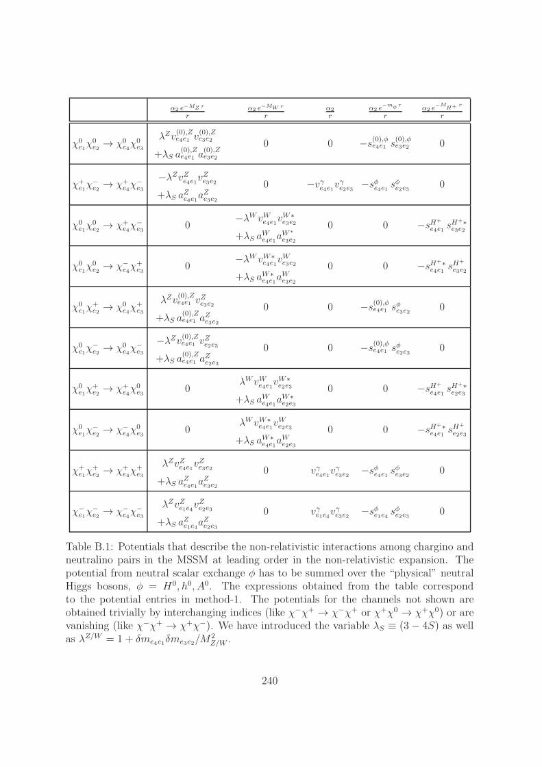
α2 e−MZ r
rα2 e−MW r
rα2
rα2 e
−mφ r
rα2 e
−MH+ r
r
χ0e1χ
0e2 → χ0
e4χ0e3
λZv(0),Ze4e1 v
(0),Ze3e2
+λS a(0),Ze4e1 a
(0),Ze3e2
0 0 −s(0),φe4e1 s(0),φe3e2 0
χ+e1χ−e2→ χ+
e4χ−e3
−λZvZe4e1vZe3e2+λS a
Ze4e1
aZe3e2
0 −vγe4e1vγe2e3 −sφe4e1 sφe2e3 0
χ0e1χ
0e2 → χ+
e4χ−e3 0
−λW vWe4e1vW∗e3e2
+λS aWe4e1a
W ∗
e3e2
0 0 −sH+
e4e1 sH+∗e3e2
χ0e1χ0e2→ χ−
e4χ+e3
0−λW vW∗
e4e1vWe3e2
+λS aW∗e4e1
aWe3e2
0 0 −sH+∗e4e1
sH+
e3e2
χ0e1χ
+e2 → χ0
e4χ+e3
λZv(0),Ze4e1 v
Ze3e2
+λS a(0),Ze4e1 a
Ze3e2
0 0 −s(0),φe4e1 sφe3e2 0
χ0e1χ−e2→ χ0
e4χ−e3
−λZv(0),Ze4e1 vZe2e3
+λS a(0),Ze4e1 a
Ze2e3
0 0 −s(0),φe4e1 sφe2e3
0
χ0e1χ+e2→ χ+
e4χ0e3
0λWvWe4e1v
W∗e2e3
+λS aWe4e1a
W∗e2e3
0 0 −sH+
e4e1sH
+∗e2e3
χ0e1χ−e2→ χ−
e4χ0e3
0λWvW∗
e4e1vWe2e3
+λS aW∗e4e1
aWe2e3
0 0 −sH+∗e4e1
sH+
e2e3
χ+e1χ+e2→ χ+
e4χ+e3
λZvZe4e1vZe3e2
+λS aZe4e1a
Ze3e2
0 vγe4e1vγe3e2
−sφe4e1 sφe3e2 0
χ−e1χ
−e2 → χ−
e4χ−e3
λZvZe1e4vZe2e3
+λS aZe1e4
aZe2e3
0 vγe1e4vγe3e2 −sφe1e4 sφe2e3 0
Table B.1: Potentials that describe the non-relativistic interactions among chargino andneutralino pairs in the MSSM at leading order in the non-relativistic expansion. Thepotential from neutral scalar exchange φ has to be summed over the “physical” neutralHiggs bosons, φ = H0, h0, A0. The expressions obtained from the table correspondto the potential entries in method-1. The potentials for the channels not shown areobtained trivially by interchanging indices (like χ−χ+ → χ−χ+ or χ+χ0 → χ+χ0) or arevanishing (like χ−χ+ → χ+χ−). We have introduced the variable λS ≡ (3− 4S) as wellas λZ/W = 1 + δme4e1δme3e2/M
2Z/W .
240
Appendix C
Equivalence between method-1 andmethod-2
In this appendix we show by means of an example, that in the formula for the Sommerfeldenhancement factors in (8.34), written in terms of annihilation matrices and wave func-tions (resulting as solutions of matrix-valued Schrodinger equations with correspondingpotential matrices) we can use either potential and annihilation matrices referring tothe method-1 basis or the corresponding method-2 expressions; the outcome will be thesame.
Instead of considering (8.34) it is more convenient for the following analysis to re-fer to the equivalent formula (8.35), where the T matrices encode the correspondinginformation on the wave functions. For the definition of the T matrix see Chap. 2.
Let us first recall from Sec. 7.2 that the method-1 two-particle basis treats as differentthe states χeaχeb and χebχea with non-identical species χea and χeb. In method-2 however,the second, redundant state χebχea – describing the same physical particle pair as thefirst state χeaχeb – is left out. We can therefore already expect that the redundancy ofcertain states in the method-1 basis translates into the corresponding solutions of theSchrodinger equation and eventually the Sommerfeld enhancement factors, while in themethod-2 calculation redundant solutions will be automatically absent.
We consider here the simple example of a system consisting of three method-1 basisstates. The first state shall be composed out of identical particles. The second andthird basis states involve two different individual particle species but are redundantwith respect to the physical particle content. The corresponding method-2 basis thuscontains only two states, the one with the two identical particles, and one of the twoother redundant method-1 states. We can think of this system as the neutral two-particle sector of the pure-wino NRMSSM: the method-1 basis states then correspond tothe three states χ0
1χ01, χ
+1 χ
−1 and χ−
1 χ+1 , while in method-2 we encounter the two neutral
basis states (χ0χ0)11 ≡ χ01χ
01 and (χ+χ−)11 ≡ χ+
1 χ−1 , see Sec. 7.2.2. Referring to this
situation we establish the generic notation χ1χ1, χ2χ3 and χ3χ2 for the three method-1basis states, with the obvious correspondence between χ1 and χ0
1 as well as similarlybetween χ2,3 and χ±
1 . The method-2 basis then contains the states (χχ)11 = χ1χ1 and
241

(χχ)23 = χ2χ3.1 For these basis states we discuss now in turn the determination of the
corresponding Sommerfeld factors (8.35) in χ1χ1 and χ2χ3 pair-annihilation reactionsrelying on potential and annihilation matrices corresponding to method-1 and method-2.
The multi-component Schrodinger equation written with respect to the method-1two-particle state basis in our example becomes a 3×3 matrix differential equation. Thecorresponding leading-order potential matrices for total spin s = 0, 1 generically read
V (1)s (r) =
V s11 V s
12 V s12
V s21 V s
22 V s23
V s21 V s
23 V s22
, (C.1)
where the first, second or third row (or column) refers to the χ1χ1, χ2χ3 or χ3χ2 state, re-spectively. For instance, the component V s
12 is given by the leading-order spin-s potentialin χ1χ1 → χ2χ3 scattering. It is worth to recall from Sec. 7.1 that a difference betweenthe spin-0 and spin-1 potentials can only arise in case of non-vanishing axial-vector cou-plings. As in the pure-wino NRMSSM all axial-vector couplings vanish, we encounteredthe same potential matrix for both cases s = 0, 1 in that scenario, see Sec. 7.2.2. Herewe will consider the generic case where V
(1)s=0(r) and V
(1)s=1(r) are not necessarily equal. In
(C.1) we have used that the potential matrix entries V s12 and V
s13 are the same. This is be-
cause the scattering reactions χ1χ1 → χ2χ3 and χ1χ1 → χ3χ2 give the same amplitudes:while the exchange of χ2χ3 by χ3χ2 corresponds to crossing the lines of the χ2 and χ3 inthe corresponding diagram, the amplitudes remain the same due to the identical particlenature of the incoming χ1χ1 state. The same reasoning obviously applies to V s
21 and Vs31.
Further we have taken into account that V s32 = V s
23 as well as V s22 = V s
33, which followsfrom the fact that the amplitudes related to the corresponding reactions differ only bya relabelling of the respective internal vertices. Finally note that the hermiticity of theunderlying MSSM Lagrangian, from which the potential interactions in the NRMSSMderive, implies the relation V s
ab = V s ∗ba .
In order to determine the Sommerfeld factors we have to construct the matrices T in(8.35) involving certain basis solutions of the corresponding radial Schrodinger equationsubject to a certain orbital angular momentum L and spin s. The radial Schrodingerequation in (2.23) can be written as
[D(L) 1+ V (1)
s (r)]~u (L,s)(r) = 0 , (C.2)
1The explicit composition of the two-particle basis states in terms of single particle constituents isto a certain extent arbitrary for our purposes here. The essential point is not the single particle contentbut the properties of the two-particle system. For instance, without reference to the neutral sector ofthe pure-wino NRMSSM we could have chosen as well the notation χ1χ1, χ1χ2, χ2χ1 for the threemethod-1 basis states. Accordingly, the method-2 basis states would then be denoted by χ1χ1 andχ1χ2. However, with the above convention for the composition of the two-particle basis states out ofindividual particles χ1,2,3, the contact to the neutral sector of the pure-wino NRMSSM discussed inSec. 6.3 and Sec. 7.2.2 becomes most apparent.
242
where we have introduced the L-dependent differential operator
D(L) =1
mLSP
[− d2
dr2+L(L+ 1)
r2−mLSPE
]. (C.3)
The matrix T is related to the three linear independent regular solutions ~u (i)(L,S)(r), i =1, 2, 3, to (C.2), see Chap. 2 and in particular (2.42). To determine the regular solutions,the structure of the potential matrix (C.1) suggests to first transform to a block-diagonal
Schrodinger equation with potential matrix V(1)s (r) defined by
V (1)s = R · V (1)
s · R† =
V s11
√2V s
11 0
√2 V s
11 V22 + V33 0
0 0 V22 − V33
. (C.4)
The constant, L- and s-independent 3× 3 matrix R is given by
R =
1 0 0
0 1√2
1√2
0 1√2− 1√
2
, (C.5)
Note that R = R† = R−1. Let us denote the three linear independent regular solutionsof the corresponding block-diagonal Schrodinger equation by ~u (i)(L,s) = R · ~u (i)(L,s). Inorder to simplify the notation, we drop in the following the indices L and s on the wavefunctions. However, it has to be kept in mind that we generically obtain different regularsolutions ~u (i=1,2,3)(r) and ~u (i=1,2,3)(r) for different pairs (L, s). Further we promote tothe matrix notation established in Chap. 2, where the regular solution vectors ~u (i) or~u (i) of the corresponding Schrodinger equation appear in the columns of 3× 3 matricesu and u. Due to the block-diagonal form of the Schrodinger equation for ~u, the solutionmatrices obtain the generic form
u =
u11 u12 0
u21 u22 0
0 0 u33
, u = R† · u =
u11 u12 0
1√2u21
1√2u22
1√2u33
1√2u21
1√2u22
−1√2u33
. (C.6)
We can now use relation (2.42) to determine the matrix T from the product of matricesu(L+1) and M−1. Without having to know the explicit form of the entries we infer from
243
(C.6), that the matrices u(L+1) and M−1 must have the generic structure
[u(L+1)L (0)] =
U11 U12 0
U21√2
U22√2
U33√2
U21√2
U22√2
−U33√2
, M =
M11 M12 0
M21√2
M22√2
M33√2
M21√2
M22√2
−M33√2
. (C.7)
Similarly this also applies to the generic structure of matrices u(L+1) and M that followsfrom u in (C.6). Note that we use capital letters to denote the (L+1)-th derivatives of therespective components of matrices u and u. The final ingredient for the determinationof the Sommerfeld factors is the corresponding method-1 annihilation matrix, whichdepends on the (L, s) quantum numbers and has the generic form
Γ(1)[2s+1LJ ] =
1+(−1)s+L
2Γ11
1+(−1)s+L
2Γ12
1+(−1)s+L
2Γ12
1+(−1)s+L
2Γ21 Γ22 (−1)s+L Γ22
1+(−1)s+L
2Γ21 (−1)s+L Γ22 Γ22
, (C.8)
as can be verified using the symmetry properties (5.9, 5.14) of the underlying Wilsoncoefficients. Further recall that Γab = Γ∗
ba. For later convenience it is worth to note thatthe transformed annihilation matrices Γ(1) = R·Γ(1) ·R† have the following generic form,distinguishing the cases where L+ s is even or odd,
Γ(1)even[
2s+1LJ ] =
Γ11
√2Γ12 0
√2Γ21 2 Γ22 0
0 0 0
, Γ
(1)odd[
2s+1LJ ] =
0 0 0
0 0 0
0 0 2 Γ22
. (C.9)
In (C.8, C.9) we suppress the labels L and s on the matrix entries Γab = Γab(2s+1LJ). To
avoid confusion let us therefore note that although the expression Γ22 appears in bothmatrices in (C.9) it does not denote the same term. In the first case the Γ22 refers to the(2, 2) entry in a corresponding matrix Γ(1)(2s+1LJ ) where L + s is even. In the secondcase the entry Γ22 is associated with a matrix Γ(1)(2s+1LJ) with odd L+ s.
It is now easy to obtain the Sommerfeld factors from (8.35). Up to a global prefactor
given by [(2L+1)!!/((L+1)! k(L+1)a )]2, the enhancement factors in annihilation reactions
of the basis states a = 1 (χ1χ1) and a = 2 (χ2χ3) subject to a 2s+1LJ partial-wavereaction with L+ s = even are given by
S even1 =
∣∣∣∣M22 U11 −M21 U12
M12M21 −M11M22
∣∣∣∣2
+ 2
∣∣∣∣M22 U21 −M21 U22
M12M21 −M11M22
∣∣∣∣2Γ22
Γ11
244
+ 2√2Re
[(M22 U21 −M21 U22) (M22 U11 −M21 U12)
∗
|M12M21 −M11M22|2Γ12
Γ11
],
S even2 =
∣∣∣∣M12 U21 −M11 U22
M12M21 −M11M22
∣∣∣∣2
+1
2
∣∣∣∣M12 U11 −M11 U12
M12M21 −M11M22
∣∣∣∣2Γ11
Γ22
+√2Re
[(M12 U21 −M11 U22) (M12 U11 −M11 U12)
∗
|M12M21 −M11M22|2Γ12
Γ22
], (C.10)
whereas for annihilation reactions of 2s+1LJ states where L+ s is odd we obtain
S odd1 = 0 ,
S odd2 =
∣∣∣∣U33
M33
∣∣∣∣2
. (C.11)
The enhancement factors for the third method-1 basis state χ3χ2 agree with the corre-sponding expressions for the second state, χ2χ3; this should be the case since both statesare physically equivalent. We observe that the enhancement factors for even L+s do notdepend on the matrix entries U33 and M33: only those wave function solutions that areassociated with the upper 2× 2 matrix in the block-diagonal Schrodinger equation withpotential (C.4) determine the enhancement factors in (C.10). To the contrary, the non-vanishing enhancement factor for odd L+s in (C.11) depends only on the wave-functionassociated with the 1 × 1 block in the block-diagonal Schrodinger equation. The factorSodd1 vanishes as two-particle configurations with L+s= odd are totally symmetric while
a state of two identical particles such as χ1χ1 has to be totally antisymmetric.Let us now turn to method-2 and construct the corresponding potential and annihi-
lation matrices. For the former we obtain, using the rules set out in Sec. 7.2.1 and thusdistinguishing even and odd L+ s,
V (2)s, even(r) =
V s11
√2V s
12
√2V s
21 V s22 + V s
23
, V
(2)s, odd(r) =
0 0
0 V s22 − V s
23
. (C.12)
In case of the annihilation matrices we have
Γ(2)even[
2s+1LJ ] =
12Γ11
1√2Γ12
1√2Γ21 Γ22
, Γ
(2)odd[
2s+1LJ ] =
0 0
0 Γ22
. (C.13)
For given orbital angular momentum L and spin s with L+ s even, the potential matrixV
(2)s agrees with the upper 2× 2 block in the corresponding V
(1)s in (C.4). Similarly the
annihilation matrices Γ(2)even correspond, up to a global factor of 2, to the upper 2 × 2
block of Γ(1)even in (C.9). From (C.6) we therefore obtain immediately the generic form of
245
the method-2 matrices [u(L+1)L (0)] and M for even L+ s:
[u(L+1)L (0)]even =
U11 U12
U21 U22
, Meven =
M11 M12
M21 M22
. (C.14)
The functions that appear for given L and s in the components of the matrices in (C.14)are the same as the Uab andMab functions with a, b = 1, 2 in the corresponding method-1matrices in (C.7).
In order to obtain the method-2 matrices [u(L+1)L (0)] and M for the case of odd L+ s
we can use the correspondence of method-2 potential and annihilation matrix entriesto the associated method-1 expressions as well. Here we find that for given (L, s) the
non-vanishing entry in the potential matrix V(2)s, odd in (C.12) agrees with the lower 1× 1
block of the corresponding matrix V(1)s in (C.4). Likewise, the non-vanishing entry in
the annihilation matrix Γ(2)odd in (C.13) agrees up to a factor of 2 with the entry in the
lower 1 × 1 block of the associated block-diagonal Γ(1)odd in (C.9). For given (L, s) with
odd L+ s we thus obtain the generic form of the matrices [u(L+1)L (0)] and M
[u(L+1)L (0)]odd =
0 0
0 U33
, Modd =
0 0
0 M33
, (C.15)
where the function U33 is the (L+ 1)-th derivative of the function u33, which appears inthe lower 1 × 1 block of the corresponding block-diagonal method-1 matrix u in (C.6),and M33 is derived from this function u33 as well.
It is now straightforward to determine for given (L, s) the Sommerfeld enhancementfactors related to pair-annihilation reactions of the first (a = 1, (χχ)11) and second(a = 2, (χχ)23) method-2 basis state. The results agree with the respective expressionsfor the Sommerfeld factors in (C.10) and (C.11), which were derived using method-1.
246

Bibliography
[1] Particle Data Group Collaboration, K. Olive et al., Chin.Phys. C38 (2014)090001.
[2] Planck Collaboration Collaboration, P. Ade et al., arXiv:1303.5076[astro-ph.CO].
[3] G. Jungman, M. Kamionkowski, and K. Griest, Phys.Rept. 267 (1996) 195–373,arXiv:hep-ph/9506380 [hep-ph].
[4] G. Bertone, D. Hooper, and J. Silk, Phys.Rept. 405 (2005) 279–390,arXiv:hep-ph/0404175 [hep-ph].
[5] P. Gondolo, J. Edsjo, P. Ullio, L. Bergstrom, M. Schelke, et al., JCAP 0407(2004) 008, arXiv:astro-ph/0406204 [astro-ph].
[6] G. Belanger, F. Boudjema, P. Brun, A. Pukhov, S. Rosier-Lees, et al.,Comput.Phys.Commun. 182 (2011) 842–856, arXiv:1004.1092 [hep-ph].
[7] J. Ellis, Nucl.Phys. A827 (2009) 187C–198C, arXiv:0902.0357 [hep-ph].
[8] D. Hooper, arXiv:0901.4090 [hep-ph].
[9] M. Cahill-Rowley, R. Cotta, A. Drlica-Wagner, S. Funk, J. Hewett, et al.,arXiv:1305.6921 [hep-ph].
[10] M. Cahill-Rowley, R. Cotta, A. Drlica-Wagner, S. Funk, J. Hewett, et al.,arXiv:1405.6716 [hep-ph].
[11] B. Herrmann and M. Klasen, Phys.Rev. D76 (2007) 117704, arXiv:0709.0043[hep-ph].
[12] B. Herrmann, M. Klasen, and K. Kovarik, Phys.Rev. D79 (2009) 061701,arXiv:0901.0481 [hep-ph].
[13] B. Herrmann, M. Klasen, and K. Kovarik, Phys.Rev. D80 (2009) 085025,arXiv:0907.0030 [hep-ph].
247
[14] J. Harz, B. Herrmann, M. Klasen, K. Kovarik, and Q. L. Boulc’h, Phys.Rev. D87(2013) no. 5, 054031, arXiv:1212.5241.
[15] B. Herrmann, M. Klasen, K. Kovarik, M. Meinecke, and P. Steppeler, Phys.Rev.D89 (2014) 114012, arXiv:1404.2931 [hep-ph].
[16] N. Baro, F. Boudjema, and A. Semenov, Phys.Lett. B660 (2008) 550–560,arXiv:0710.1821 [hep-ph].
[17] N. Baro, F. Boudjema, and A. Semenov, Phys.Rev. D78 (2008) 115003,arXiv:0807.4668 [hep-ph].
[18] N. Baro, F. Boudjema, G. Chalons, and S. Hao, Phys.Rev. D81 (2010) 015005,arXiv:0910.3293 [hep-ph].
[19] J. Hisano, S. Matsumoto, M. M. Nojiri, and O. Saito, Phys.Rev. D71 (2005)063528, arXiv:hep-ph/0412403 [hep-ph].
[20] J. Hisano, S. Matsumoto, M. Nagai, O. Saito, and M. Senami, Phys.Lett. B646(2007) 34–38, arXiv:hep-ph/0610249 [hep-ph].
[21] M. Drees, J. Kim, and K. Nagao, Phys.Rev. D81 (2010) 105004,arXiv:0911.3795 [hep-ph].
[22] A. Hryczuk, R. Iengo, and P. Ullio, JHEP 1103 (2011) 069, arXiv:1010.2172[hep-ph].
[23] A. Hryczuk, Phys.Lett. B699 (2011) 271–275, arXiv:1102.4295 [hep-ph].
[24] A. Hryczuk and R. Iengo, JHEP 1201 (2012) 163, arXiv:1111.2916 [hep-ph].
[25] J. Fan and M. Reece, JHEP 1310 (2013) 124, arXiv:1307.4400 [hep-ph].
[26] T. Cohen, M. Lisanti, A. Pierce, and T. R. Slatyer, JCAP 1310 (2013) 061,arXiv:1307.4082.
[27] A. Hryczuk, I. Cholis, R. Iengo, M. Tavakoli, and P. Ullio, JCAP 1407 (2014) 031,arXiv:1401.6212 [astro-ph.HE].
[28] M. Cirelli, A. Strumia, and M. Tamburini, Nucl.Phys. B787 (2007) 152–175,arXiv:0706.4071 [hep-ph].
[29] N. Arkani-Hamed, D. P. Finkbeiner, T. R. Slatyer, and N. Weiner, Phys.Rev. D79(2009) 015014, arXiv:0810.0713 [hep-ph].
[30] G. T. Bodwin, E. Braaten, and G. P. Lepage, Phys.Rev. D51 (1995) 1125–1171,arXiv:hep-ph/9407339 [hep-ph].
248

[31] M. Beneke, C. Hellmann, and P. Ruiz-Femenia, JHEP 1303 (2013) 148,arXiv:1210.7928 [hep-ph].
[32] C. Hellmann and P. Ruiz-Femenia, JHEP 1308 (2013) 084, arXiv:1303.0200[hep-ph].
[33] M. Beneke, C. Hellmann, and P. Ruiz-Femenia, arXiv:1411.6924 [hep-ph].
[34] M. Beneke, C. Hellmann, and P. Ruiz-Femenia, arXiv:1411.6930 [hep-ph].
[35] M. Beneke and V. A. Smirnov, Nucl.Phys. B522 (1998) 321–344,arXiv:hep-ph/9711391 [hep-ph].
[36] T. R. Slatyer, JCAP 1002 (2010) 028, arXiv:0910.5713 [hep-ph].
[37] R. Iengo, JHEP 0905 (2009) 024, arXiv:0902.0688 [hep-ph].
[38] S. Cassel, J.Phys. G37 (2010) 105009, arXiv:0903.5307 [hep-ph].
[39] S. Hannestad and T. Tram, JCAP 1101 (2011) 016, arXiv:1008.1511[astro-ph.CO].
[40] J. L. Feng, M. Kaplinghat, and H.-B. Yu, Phys.Rev. D82 (2010) 083525,arXiv:1005.4678 [hep-ph].
[41] F. Brau and F. Buisseret, Phys.Rev. C76 (2007) 065212, arXiv:0706.4012[hep-ph].
[42] K. L. McDonald, JHEP 1207 (2012) 145, arXiv:1203.6341 [hep-ph].
[43] Z. Zhang, arXiv:1307.2206 [hep-ph].
[44] B. W. Lee and S. Weinberg, Phys.Rev.Lett. 39 (1977) 165–168.
[45] J. Bernstein, L. S. Brown, and G. Feinberg, Phys.Rev. D32 (1985) 3261.
[46] R. J. Scherrer and M. S. Turner, Phys.Rev. D33 (1986) 1585.
[47] M. Srednicki, R. Watkins, and K. A. Olive, Nucl.Phys. B310 (1988) 693.
[48] K. Griest and D. Seckel, Phys.Rev. D43 (1991) 3191–3203.
[49] P. Gondolo and G. Gelmini, Nucl.Phys. B360 (1991) 145–179.
[50] E. W. Kolb and M. S. Turner, Front.Phys. 69 (1990) 1–547.
[51] T. Bringmann and S. Hofmann, JCAP 0407 (2007) 016, arXiv:hep-ph/0612238[hep-ph].
249
[52] J. B. Dent, S. Dutta, and R. J. Scherrer, Phys.Lett. B687 (2010) 275–279,arXiv:0909.4128 [astro-ph.CO].
[53] J. Edsjo and P. Gondolo, Phys.Rev. D56 (1997) 1879–1894,arXiv:hep-ph/9704361 [hep-ph].
[54] M. Hindmarsh and O. Philipsen, Phys.Rev. D71 (2005) 087302,arXiv:hep-ph/0501232 [hep-ph].
[55] H. Georgi and S. Glashow, Phys.Rev.Lett. 32 (1974) 438–441.
[56] H. E. Haber and G. L. Kane, Phys.Rept. 117 (1985) 75–263.
[57] S. P. Martin, Adv.Ser.Direct.High Energy Phys. 21 (2010) 1–153,arXiv:hep-ph/9709356 [hep-ph].
[58] M. Drees, R. Godbole, and P. Roy.
[59] I. J. Aitchison, arXiv:hep-ph/0505105 [hep-ph].
[60] D. Z. Freedman and A. Van Proeyen.
[61] J. Gunion and H. E. Haber, Nucl.Phys. B272 (1986) 1.
[62] J. Rosiek, Phys.Rev. D41 (1990) 3464, arXiv:hep-ph/9511250 [hep-ph].Erratum: ibid. vol. 387, p. 830 (1997).
[63] G. R. Farrar and P. Fayet, Phys.Lett. B76 (1978) 575–579.
[64] M. Dine and A. E. Nelson, Phys.Rev. D48 (1993) 1277–1287,arXiv:hep-ph/9303230 [hep-ph].
[65] M. Dine, A. E. Nelson, and Y. Shirman, Phys.Rev. D51 (1995) 1362–1370,arXiv:hep-ph/9408384 [hep-ph].
[66] M. Dine, A. E. Nelson, Y. Nir, and Y. Shirman, Phys.Rev. D53 (1996) 2658–2669,arXiv:hep-ph/9507378 [hep-ph].
[67] G. Giudice and R. Rattazzi, Phys.Rept. 322 (1999) 419–499,arXiv:hep-ph/9801271 [hep-ph].
[68] L. Randall and R. Sundrum, Nucl.Phys. B557 (1999) 79–118,arXiv:hep-th/9810155 [hep-th].
[69] L. Girardello and M. T. Grisaru, Nucl.Phys. B194 (1982) 65.
[70] R. Barbieri, S. Ferrara, and C. A. Savoy, Phys.Lett. B119 (1982) 343.
[71] A. H. Chamseddine, R. L. Arnowitt, and P. Nath, Phys.Rev.Lett. 49 (1982) 970.
250
[72] S. Choi, M. Guchait, J. Kalinowski, and P. Zerwas, Phys.Lett. B479 (2000)235–244, arXiv:hep-ph/0001175 [hep-ph].
[73] S. Choi, J. Kalinowski, G. A. Moortgat-Pick, and P. Zerwas, Eur.Phys.J. C22(2001) 563–579, arXiv:hep-ph/0108117 [hep-ph].
[74] J. F. Gunion and H. E. Haber, Phys.Rev. D37 (1988) 2515.
[75] H.-C. Cheng, B. A. Dobrescu, and K. T. Matchev, Nucl.Phys. B543 (1999) 47–72,arXiv:hep-ph/9811316 [hep-ph].
[76] D. Pierce and A. Papadopoulos, Phys.Rev. D50 (1994) 565–570,arXiv:hep-ph/9312248 [hep-ph].
[77] D. Pierce and A. Papadopoulos, Nucl.Phys. B430 (1994) 278–294,arXiv:hep-ph/9403240 [hep-ph].
[78] G. F. Giudice and A. Pomarol, Phys.Lett. B372 (1996) 253–258,arXiv:hep-ph/9512337 [hep-ph].
[79] A. Lahanas, K. Tamvakis, and N. Tracas, Phys.Lett. B324 (1994) 387–396,arXiv:hep-ph/9312251 [hep-ph].
[80] D. M. Pierce, J. A. Bagger, K. T. Matchev, and R.-j. Zhang, Nucl.Phys. B491(1997) 3–67, arXiv:hep-ph/9606211 [hep-ph].
[81] A. Chatterjee, M. Drees, S. Kulkarni, and Q. Xu, Phys.Rev. D85 (2012) 075013,arXiv:1107.5218 [hep-ph].
[82] S. Heinemeyer, F. von der Pahlen, and C. Schappacher, Eur.Phys.J. C72 (2012)1892, arXiv:1112.0760 [hep-ph].
[83] A. Bharucha, S. Heinemeyer, F. von der Pahlen, and C. Schappacher, Phys.Rev.D86 (2012) 075023, arXiv:1208.4106 [hep-ph].
[84] A. Bharucha, A. Fowler, G. Moortgat-Pick, and G. Weiglein, JHEP 1305 (2013)053, arXiv:1211.3134 [hep-ph].
[85] T. Fritzsche, T. Hahn, S. Heinemeyer, H. Rzehak, and C. Schappacher,arXiv:1309.1692 [hep-ph].
[86] A. Djouadi, J.-L. Kneur, and G. Moultaka, Comput.Phys.Commun. 176 (2007)426–455, arXiv:hep-ph/0211331 [hep-ph].
[87] B. Allanach and M. Bernhardt, Comput.Phys.Commun. 181 (2010) 232–245,arXiv:0903.1805 [hep-ph].
[88] W. Porod and F. Staub, Comput.Phys.Commun. 183 (2012) 2458–2469,arXiv:1104.1573 [hep-ph].
251
[89] J. Alwall, M. Herquet, F. Maltoni, O. Mattelaer, and T. Stelzer, JHEP 1106(2011) 128, arXiv:1106.0522 [hep-ph].
[90] R. Cutkosky, J.Math.Phys. 1 (1960) 429–433.
[91] G. ’t Hooft and M. Veltman, NATO Sci.Ser.B 4 (1974) 177–322.
[92] A. Denner, H. Eck, O. Hahn, and J. Kublbeck, Nucl.Phys. B387 (1992) 467–484.
[93] M. Drees and J. Gu, Phys.Rev. D87 (2013) no. 6, 063524, arXiv:1301.1350[hep-ph].
[94] J. Chen and Y.-F. Zhou, JCAP 1304 (2013) 017, arXiv:1301.5778 [hep-ph].
[95] J. F. Gunion and H. E. Haber, Phys.Rev. D67 (2003) 075019,arXiv:hep-ph/0207010 [hep-ph].
[96] M. Drees and M. M. Nojiri, Phys.Rev. D47 (1993) 376–408,arXiv:hep-ph/9207234 [hep-ph].
[97] S. Ershov, J. Vaagen, and M. Zhukov, Phys.Rev. C84 (2011) 064308.
[98] M. W. Cahill-Rowley, J. L. Hewett, A. Ismail, M. E. Peskin, and T. G. Rizzo,arXiv:1305.2419 [hep-ph].http://www.slac.stanford.edu/~aismail/snowmass/index.html.
252
Acknowledgements
I am grateful to my advisor Martin Beneke for his supervision in the last years andthe many valuable and encouraging discussions. Further, I would like to thank MartinBeneke and Pedro Ruiz-Femenia for the fruitful collaboration on the dark matter project.In addition, I want to thank Pedro Ruiz-Femenia for careful reading of the manuscriptof this thesis and many helpful comments.
I thank Jan Piclum for his comments on parts of the manuscript as well as fora lot of useful discussions. Furthermore I would like to thank the members of theTheoretical Particle Physics Department T31 at the Technische Universitat Munchenfor the encouraging and pleasant working atmosphere.
Finally, I am particularly grateful to the Deutsche Telekom Stiftung and to theStudienstiftung des deutschen Volkes for their generous ideationally and financial sup-port.
253


Annihilation matrices in pair annihilations ofnon-relativistic neutralinos and charginos:documentation of the numerical program
Charlotte Hellmann
26.02.2015
Abstract
We provide a documentation of the numerical code that determines the partial-waveseparated annihilation matrix expressions in non-relativistic neutralino and charginopair-annihilation reactions in the general MSSM.

ii
Contents
1 Introduction 2
2 Generic structure of the code 3
3 Part 1: Building the partial wave coefficients 6
3.1 Kinematic factors . . . . . . . . . . . . . . . . . . . . . . . . . . . . . . . 63.1.1 Selfenergy topologies . . . . . . . . . . . . . . . . . . . . . . . . . 73.1.2 Triangle topologies . . . . . . . . . . . . . . . . . . . . . . . . . . 93.1.3 Box topologies . . . . . . . . . . . . . . . . . . . . . . . . . . . . 10
3.2 Coupling factors . . . . . . . . . . . . . . . . . . . . . . . . . . . . . . . . 113.2.1 Selfenergy diagrams . . . . . . . . . . . . . . . . . . . . . . . . . . 113.2.2 Triangle diagrams . . . . . . . . . . . . . . . . . . . . . . . . . . . 143.2.3 Box diagrams . . . . . . . . . . . . . . . . . . . . . . . . . . . . . 15
3.3 Partial wave coefficients: generic routine . . . . . . . . . . . . . . . . . . 153.3.1 The function PartialWaveCoefficient[...] . . . . . . . . . . . 163.3.2 Auxiliary functions in partialwavecoefficients.m . . . . . . . 18
3.4 Partial wave coefficients: physical reactions . . . . . . . . . . . . . . . . . 193.4.1 Listing internally exchanged states . . . . . . . . . . . . . . . . . 193.4.2 The function pwc[...] related to the physical exclusive process . 22
4 Part 2: Building the annihilation matrices 23
4.1 Enumeration convention for χχ states . . . . . . . . . . . . . . . . . . . . 244.2 The choice of the mass expansion . . . . . . . . . . . . . . . . . . . . . . 254.3 Inclusive reactions: the final partial wave coefficients . . . . . . . . . . . 264.4 Symmetry factors and symmetry relations . . . . . . . . . . . . . . . . . 284.5 Chopping numerically small annihilation matrix entries . . . . . . . . . . 294.6 Calculation of the annihilation matrices . . . . . . . . . . . . . . . . . . . 29
5 Comparison to the publications’ nomenclature 32
5.1 Kinematic and coupling factors . . . . . . . . . . . . . . . . . . . . . . . 325.2 Annihilation matrices . . . . . . . . . . . . . . . . . . . . . . . . . . . . . 33
1

1 Introduction
We provide a documentation of the numerical code that allows to calculate the annihi-lation matrices in pair-annihilation reactions of non-relativistic neutralino and charginopairs including O(v2rel) effects in the non-relativistic expansion and at leading order in theexpansion in the couplings. The annihilation matrices are built from the absorptive partsof Wilson coefficients of four-fermion operators. The latter encode the hard annihilationreactions of non-relativistic neutralinos and charginos in the NRMSSM, an effective fieldtheory designed to determine the enhanced radiative corrections in neutralino/charginoco-annihilation processes.
The construction of the NRMSSM is described in detail in [1–4] as well as in thepreceeding thesis. The first two publications [1, 2]1 cover the determination of the Wil-son coefficients encoding the hard annihilation reactions, while the third focuses on thetechnical aspects in the calculation of the Sommerfeld enhancements. In [4] a dedicateddiscussion of several MSSM benchmark scenarios in view of the impact of Sommerfeldenhancements in the χ0
1 relic abundance is given. For the underlying physics and tech-nical aspects of the calculation we refer the reader to [1–3]. This documentation dealsexclusively with the numerical code that determines the annihilation matrices.
The outline of this documentation is as follows. Sec. 2 contains a general overviewon the structure of the code, which can be divided into two main parts with respectiveextensive substructure. Part 1 of the code refers to elementary functions and buildingblocks related to the construction of the partial wave separated Wilson coefficients.Consequently, part 2 deals with the construction of annihilation matrices, thereby relyingon functions that are the subject-matter of part 1.
The first part of the code is described in detail in Sec. 3. Starting with the basic build-ing blocks, Sec. 3.1 and Sec. 3.2 cover the hard-coded kinematic and coupling factors.The generic functions that allow to determine a specific exclusive final state contributionto the absorptive part of a Wilson coefficient from the kinematic and coupling factorsare then described in Sec. 3.3. In Sec. 3.4 a description of necessary hard-coded infor-mation is given that allows to determine partial wave coefficient contributions related toscattering reactions with exclusive physical final states.
The second part of the code is the subject-matter of Sec. 4 and deals with the func-tions determining the annihilation matrices, which are related to non-relativistic neu-tralino and chargino pair-annihilation reactions. Sec. 4.1 introduces the enumerationconvention for the neutralino and chargino pairs (χχ pairs) that we have chosen in boththe numerical ”annihilation matrix” and ”Sommerfeld enhancement” programs.2 Theenumeration convention for the χχ pairs fixes the position (row and column) where thecontributions from a specific χχ annihilation reaction appear in the annihilation matri-ces. The question which version of the hard-coded kinematic factors should be chosen for
1All conventions and definitions in [1,2] and the thesis agree, such that regarding the contents of [1,2]the reader may refer to Chaps. 5 and 6 of the thesis as well.
2This documentation deals exclusively with the piece of the code determining the short-distanceannihilation matrices, that is the ”annihilation matrix” program.
2
a specific annihilation reaction as regards the expansion in mass differences is addressedin Sec. 4.2. Subsequently, in Sec. 4.3, we introduce the functions that determine theabsorptive parts of the proper Wilson coefficients, referring to the inclusive annihilationreactions. The issue of symmetry factors and relations among certain Wilson coefficientfunctions defined in the code is the content of Sec. 4.4. The following Sec. 4.5 introducesa convenient function that allows to sets to zero annihilation matrix entries that are verysmall compared to the leading annihilation matrix entries. The functions that determinethe final annihilation matrix expressions are described in Sec. 4.6.
For the sake of clarity, those expressions are summarised in Sec. 5, whose definition ornomenclature in the numerical program is slightly different with respect to the definitionor naming established in [1–4].
2 Generic structure of the code
The numeric code is designed to calculate all diagonal and off-diagonal hard annihilationrates in co-annihilation reactions of non-relativistic and nearly mass-degenerate neu-tralino and chargino pairs including O(v2rel) corrections in the non-relativistic expansion.While in the current version of the code the final expressions for the annihilation ma-trices refer to the respective inclusive annihilation rates, all contributing exclusive ratesare determined in intermediate steps.3 By appropriate and easily implementable modi-fications in the current version of the code it is therefore possible to obtain annihilationmatrices referring to exclusive final states.
The code relies on the explicit calculation of the absorptive parts of the (partial-waveseparated) Wilson coefficients of four fermion operators in the NRMSSM at leadingorder, O(α2
2), in the expansion in the couplings. We use α2 = g22/4π where g2 denotesthe SU(2)L gauge coupling. For the explicit form of the four-fermion operators we referthe reader to [1, 2] or to the thesis. According to the latter references, the Wilsoncoefficients corresponding to the four-fermion operators can be written in terms of a sumover products of kinematic and coupling factors. Schematically, the absorptive part ofa Wilson coefficient f can therefore be obtained from a suitable set of kinematic andcoupling factors as
f =∑
coupling factor× kinematic factor . (1)
The definition of the four-fermion operators and their Wilson coefficients as given in[1, 2] and the thesis and as underlying the numerical code described herein is the same.Therefore the expression for a Wilson coefficient can be unambiguously obtained eitherfollowing the prescriptions given in [1,2] or from the code described hereafter. However,the definition of the kinematic and the coupling factors is not identical in [1, 2] and thenumerical code. For instance, in the convention of [1, 2] a sign can be associated with a
3Let us note that the calculated hard annihilation rates refer to the annihilation reactions at tree-level, such that exclusive rates are infrared safe and can be given separately.
3

specific kinematic factor appearing in the sum (1). In the conventions of the numericalcode, the sign can be absent in front of the kinematic factor but will then be attributedto the corresponding coupling factor. As a consequence, the expression for the Wilsoncoefficient stays always the same. Such difference between kinematic and coupling factorexpressions in [1, 2] and the numerical code originates from the fact that the referenceprocesses used in the determination of the kinematic and coupling factors for [1, 2] andin the code are different. The reader should be aware of this difference, implying thatintermediate results obtained from expressions in [1,2] or from the numerical code cannotbe used interchangeably. The end result, which is the Wilson coefficient, is unambiguous,also in case of exclusive final state reactions.
Once more, to make the above explicit, note the following: [1,2] and the thesis containexplicit analytic results for the kinematic factors associated with leading order 1S0- and3S1-wave Wilson coefficients as well as analytic results for the kinematic factors related to1P1 and
3PJ partial-wave annihilations. The 3PJ -wave Wilson coefficients are a suitablelinear combination of the respective three corresponding P -wave coefficients associatedwith spin S = 1, see [2] or eq. (6.29) in the thesis. The code uses an equivalent set ofkinematic factors calculated in the same way as the corresponding expressions in [1, 2]and the thesis. However, the kinematic factors given in [1, 2] and Appendix A of thethesis are not identical to the kinematic factors used in the code. In both cases we useda certain reference process χe1χe2 → XAXB → χe4χe3 to determine the kinematic andcoupling factors that built the Wilson coefficients. For instance, in case of final statesXAXB built from two gauge bosons, the kinematic factors used in the code rely on thereference process χ0
e1χ0e2
→ W+W− → χ0e4χ0e3. To the contrary, we used the reference
process χe1χe2 → V V → χe4χe3 , where χei denote generic Majorana fermions and V ageneric gauge boson in the calculation referring to [1, 2]. Similar small differences existfor the other processes. Results on the kinematic and coupling factors can therefore notbe used interchangeably in the code and the publications. Each calculation is howeverself-consistent and the final results on the Wilson coefficients encoding physical ratesare identical. A list of reference processes underlying the results for the kinematic andcoupling factors used in the numerical code is provided at the end of Sec. 3.1. Takingthese reference processes into account and following the generic steps for the kinematicand coupling factor construction described in [1, 2] or Chap. 6 and Appendix A of thethesis, the reader can reproduce the kinematic and coupling factors expressions that arehard-coded in the numerical code.
Conceptually the code is divided into two parts where the first refers to the deter-mination of the Wilson coefficients and the second is subsequently associated with theconstruction of the annihilation matrices from the former results. Part 1 and part 2 relyon different Mathematica “.m” files introduced in the following.
1. a. Within part 1, the following Mathematica “.m” file contains hard-coded resultsfor the kinematic factors used in the code:
kinfactors Code.m .
4

This includes all results referring to box, triangle and selfenergy diagrams. Wediscuss the structure of the kinematic factors in Sec. 3.1.
b. The corresponding hard-coded coupling factor results are collected in the threefiles
couplingFactors boxes.m,
couplingFactors triangles.m,
couplingFactors selfenergies.m.
A closer description of the above files is given in Sec. 3.2.
c. The generic routines that build the different box-, triangle- and selfenergy-diagram contributions to a Wilson coefficient from the kinematic and couplingfactors are contained in
partialwavecoefficients.m
and will be discussed in more detail in Sec. 3.3.
d. In order to build the specific χe1χe2 → XAXB → χe4χe3 contribution to acertain Wilson coefficient that refers to the inclusive χe1χe2 →
∑
XAXB → χe4χe3
reaction, we have to further specify which particles are exchanged internally in thes-, t- or u-channels of the respective selfenergy, triangle or box diagrams. This isneeded because the kinematic and coupling factor expressions are still generic in thesense that they use place-holder masses and indices referring to a certain neutralinoor chargino state. The latter have to be set to the corresponding particle massesand indices when a specific Wilson coefficient is determined. For each possibleexclusive reaction the information on the internally exchanged particles in the box,triangle and selfenergy amplitudes is collected in the files
scatteringchannels boxes.m ,scatteringchannels triangles.m ,scatteringchannels self.m .
When building the Wilson coefficients with the help of the functions defined inpartialwavecoefficients.m, the information encoded in the latter files is used.The nomenclature of the hard-coded lists in the above scatteringchannels xxx.m
files is given in Sec. 3.4. In addition, this section contains the description of thefunctions written in
partialwavecoefficients channels.m ,
which contain the definition of the Wilson coefficient contributions referring toexclusive physical tree-level annihilation reactions χe1χe2 → XAXB → χe4χe3 .
5
2. Part 2 of the code, dealing with the construction of the annihilation matrices, isbased on the functions collected in the file
annihilationmatrices vx.m
where x is a place-holder for the version number. The current version is x=7.Details on the functions and definitions related to this part are given in Sec. 4.
3 Part 1: Building the partial wave coefficients
3.1 Kinematic factors
As described in [1, 2] and in the preceeding thesis in Sec. 6.1.4, the Wilson coefficientof a NRMSSM four-fermion operator is given by a sum over products of kinematicand coupling factors. The numerical code comes with hard-coded expressions for thekinematic and coupling factors that refer to all relevant box, triangle and selfenergyamplitudes. As stated in Sec. 2 above, the conventions underlying the definitions ofkinematic and coupling factors are different in [1, 2] and the code, while the outcomefor the partial-wave coefficients agrees. We discuss the structure of the code’s kinematicfactor expressions in this section and subsequently describe in Sec. 3.2 the form of thecorresponding coupling factors.
Within the numerical code, the hard-coded kinematic factor expressions are collectedin the file kinfactors Code.m. Also the nomenclature in the code differs slightly fromthe one in the publications. The code’s kinematic factors referring to a selfenergy topol-ogy have the generic structure
kE[n,"chi chi -> (i1) -> XA XB -> (i2) -> chi chi",2s+1LJ,mci,alpha]. (2)
In case of triangle topologies the following nomenclature is used
kD[n, "chi -> (X) -> XA XB -> chi chi", 2s+1LJ, mci, alpha] , (3)
and box topologies are referred to as
kC[n, "chi chi -> XA XB -> chi chi", 2s+1LJ, mci, alpha] . (4)
In the above expressions the terms XA XB, 2s+1LJ and mci denote place-holders thatcan be set to the following values
• XA XB refers to the type of particles XA and XB in the final state of a χχ → XAXB
annihilation reaction. Both XA and XB can be given by a vector boson (V ),scalar (S), fermion (f) or a ghost (η). Taking all possible two-particle final statecombinations into account the argument XA XB in the code can be given the values
XA XB =
V V (V V final state)V S (V S final state)S S (SS final state)f fbar (ff final state)gh gh (ηη final state) .
6
• 2s+1LJ specifies the partial wave configuration and is given by one of the fol-lowing strings
2s+1LJ =
"1S0","3S1", for leading order S-wave coefficients,"1P1","3Px", for 1P1 and the combined 3PJ coefficients,"3P0","3P1", "3P2", for the individual 3PJ=0,1,2 coefficients,"1S0,p2","3S1,p2", for p2 proportional nnlo S-wave coeff.,"1S0,dm","3S1,dm", for δm proportional S-wave coeff.,"1S0,dmbar","3S1,dmbar", for δm proportional S-wave coeff..
Let us recall that the absorptive part of a 3PJ Wilson coefficient f is obtainedfrom the spin-1 P -wave Wilson coefficients by the following linear combination
f(
3PJ
)
=1
3f(
3P0
)
+1
3f(
3P1
)
+5
3f(
3P2
)
. (5)
The corresponding kinematic factor expressions obviously obtain from the samelinear combination.
• mci specifies which expansion in mass differences is chosen. It can be set to thetwo values mci = mc1, mc2. For a discussion on the two possible expansions inmass differences we refer the reader to [1, 2] or Sec. 6.1.2 in the thesis.
The further arguments of the kinematic factors kE[...], kD[...] and kC[...] abovediffer for differing topology. We discuss these arguments for each topology in turn inSec. 3.1.1 – 3.1.3
In order to determine the kinematic factor expressions used in the numerical codewe have calculated the box, triangle and selfenergy amplitudes in processes χ0
e1χ0e2
→XAXB → χ0
e4χ0e3
with XAXB given by
W+W− serving as reference for V V final states,
W+G− for V S final states,
G+G− for SS final states,
uI uJ for SS final states.
(6)
Here the superscripts I, J indicate the family index for the SM up-type quarks. Thesteps to be followed in the calculation of the code’s kinematic factors can be found in [1]or Sec. 6.1.2 – 6.1.4 of the thesis. In the latter also the reference processes used in thecalculation of the kinematic factors in [1, 2] and the thesis are given.
3.1.1 Selfenergy topologies
The generic form of a selfenergy diagram in χχ → XAXB → χχ scattering is given inFig. 1. In case of the kinematic factors kE[...] related to such selfenergy topology thearguments n, i1, i2, and alpha can get the following inputs:
7

XA
selfenergy (ss)
XBχe1
χe4
χe3
χe2
Figure 1: Generic selfenergy diagram in χχ → XAXB → χχ reactions, with XA andXB representing any two-body final state of SM and Higgs particles. The shorthand ssnotation indicates that the selfenergy amplitude corresponds to two s-channel exchangetree-level diagrams that are associated with χe1χe2 → XAXB and χe4χe3 → XAXB
annihilations, respectively. (Also see Fig. 9, 10 in paper I and Fig. A.1, A.2 in thethesis).
• n refers to a character string that contains information on the type of couplings atthe vertices of the selfenergy diagram. It can be set to
n = "rr","pp" for XA XB = V V, V S, S S, gh gh.
The first (second) character in this two-character string refers to the type of coup-ling at the vertex that involves the incoming χe1χe2 pair (the outgoing χe4χe3 pair)in the selfenergy diagram referring to the χe1χe2 → XAXB → χe4χe3 reaction.While r indicates a coupling of either vector or scalar type, the character p refersto a coupling of axial-vector or pseudo-scalar type. The couplings of the inter-mediate particles in the selfenergy amplitude are fixed once XA XB and i1,i2 arespecified and therefore do not need to be indicated in the string n. However incase of selfenergy diagrams with XAXB = ff the type of coupling of the final statefermions XAXB to the s-channel exchanged particles needs to be specified. In thiscase
n = "rr rr","rr pp","pp rr","pp pp" for XA XB = f fbar.
Here, the character r or p at the first (second) position in the string indicates thetype of coupling of the incoming χe1χe2 (outgoing χe4χe3) pair to the respective s-channel exchanged particle. Similarly, the character at the third (fourth) positionin the string n refers to the type of coupling between the final state fermionsXAXB and the particle exchanged in the left (right) single s-channel. As beforeand throughout the character r is used to refer to a vector or scalar coupling andp indicates a coupling of axial-vector or pseudo-scalar type.
• i1, i2 are given by either V or S. These inputs denote the particle species – vectorboson V or scalar S – that is exchanged in the left (i1) or right (i2) single s-channelof the corresponding selfenergy amplitude.
8
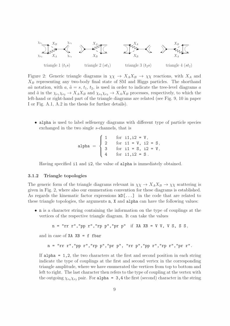
XA
triangle 1 (t1s)
XB
triangle 3 (t2s) triangle 4 (st2)triangle 2 (st1)
XAXBXB
XBXAXAχe1
χe4
χe3
χe2
Figure 2: Generic triangle diagrams in χχ → XAXB → χχ reactions, with XA andXB representing any two-body final state of SM and Higgs particles. The shorthandaa notation, with a, a = s, t1, t2, is used in order to indicate the tree-level diagrams aand a in the χe1χe2 → XAXB and χe4χe3 → XAXB processes, respectively, to which theleft-hand or right-hand part of the triangle diagrams are related (see Fig. 9, 10 in paperI or Fig. A.1, A.2 in the thesis for further details).
• alpha is used to label selfenergy diagrams with different type of particle speciesexchanged in the two single s-channels, that is
alpha =
1 for i1,i2 = V ,2 for i1 = V, i2 = S ,3 for i1 = S, i2 = V ,4 for i1,i2 = S .
Having specified i1 and i2, the value of alpha is immediately obtained.
3.1.2 Triangle topologies
The generic form of the triangle diagrams relevant in χχ → XAXB → χχ scattering isgiven in Fig. 2, where also our enumeration convention for these diagrams is established.As regards the kinematic factor expressions kD[...] in the code that are related tothese triangle topologies, the arguments n, X and alpha can have the following values:
• n is a character string containing the information on the type of couplings at thevertices of the respective triangle diagram. It can take the values
n = "rr r","pp r","rp p","pr p" if XA XB = V V, V S, S S ,
and in case of XA XB = f fbar
n = "rr r","pp r","rp p","pr p", "rr p","pp r","rp r","pr r".
If alpha = 1,2, the two characters at the first and second position in each stringindicate the type of couplings at the first and second vertex in the correspondingtriangle amplitude, where we have enumerated the vertices from top to bottom andleft to right. The last character then refers to the type of coupling at the vertex withthe outgoing χe4χe3 pair. For alpha = 3,4 the first (second) character in the string
9
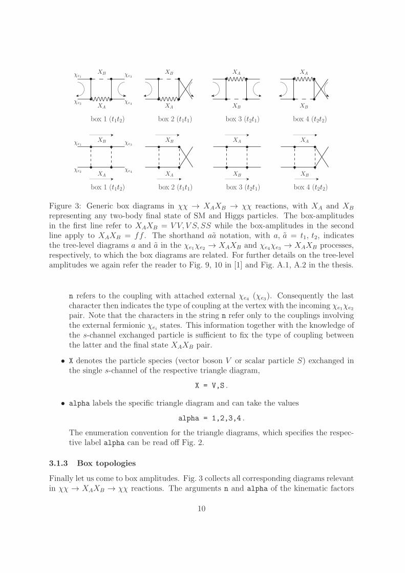
XA
box 1 (t1t2)
XB XB XA XA
XA XB
box 3 (t2t1) box 4 (t2t2)box 2 (t1t1)
XB
χe1
χe2
χe3
χe4
XA
box 1 (t1t2)
XB XB XA XA
XA XB
box 3 (t2t1) box 4 (t2t2)box 2 (t1t1)
XB
χe1
χe2
χe3
χe4
Figure 3: Generic box diagrams in χχ → XAXB → χχ reactions, with XA and XB
representing any two-body final state of SM and Higgs particles. The box-amplitudesin the first line refer to XAXB = V V, V S, SS while the box-amplitudes in the secondline apply to XAXB = ff . The shorthand aa notation, with a, a = t1, t2, indicatesthe tree-level diagrams a and a in the χe1χe2 → XAXB and χe4χe3 → XAXB processes,respectively, to which the box diagrams are related. For further details on the tree-levelamplitudes we again refer the reader to Fig. 9, 10 in [1] and Fig. A.1, A.2 in the thesis.
n refers to the coupling with attached external χe4 (χe3). Consequently the lastcharacter then indicates the type of coupling at the vertex with the incoming χe1χe2
pair. Note that the characters in the string n refer only to the couplings involvingthe external fermionic χei states. This information together with the knowledge ofthe s-channel exchanged particle is sufficient to fix the type of coupling betweenthe latter and the final state XAXB pair.
• X denotes the particle species (vector boson V or scalar particle S) exchanged inthe single s-channel of the respective triangle diagram,
X = V,S .
• alpha labels the specific triangle diagram and can take the values
alpha = 1,2,3,4 .
The enumeration convention for the triangle diagrams, which specifies the respec-tive label alpha can be read off Fig. 2.
3.1.3 Box topologies
Finally let us come to box amplitudes. Fig. 3 collects all corresponding diagrams relevantin χχ → XAXB → χχ reactions. The arguments n and alpha of the kinematic factors
10
kC[...] related to these box amplitudes read as follows:
• n is a four-character string where the ith character refers to the coupling at theith vertex of the box amplitude. Here the vertices of the box amplitudes areenumerated according to the respective attached external particles χei, i = 1, . . . , 4.The string n can take the form
n = "rrrr","pppp","rrpp","pprr","rppr","prrp","rprp","prpr" .
• alpha labels the four box diagrams,
alpha = 1,2,3,4 ,
where our enumeration convention for the box diagrams can be read off Fig. 3.
3.2 Coupling factors
When the three files couplingFactors boxes.m, couplingFactors triangles.m andcouplingFactors selfenergies.m are loaded in a Mathematica session, coupling factorexpressions will be constructed that together with the corresponding kinematic factorsdescribed in the previous section will finally allow to build the absorptive part f ofWilson coefficients related to a specific χe1χe2 → XAXB → χe4χe3 reaction. In thissection we discuss the nomenclature of the coupling factors used in the numerical codeand describe the functions that determine these expressions from specific hard-codedlists. The latter contain the coupling factors that occur at each vertex of a specific box,triangle or selfenergy amplitude.
3.2.1 Selfenergy diagrams
Coupling factors corresponding to selfenergy diagrams have the generic form
eC[n, "chi chi -> (i1) -> XA XB -> (i2) -> chi chi", alpha] . (7)
The arguments n and alpha of the expression eC[...] take the same values as thecorresponding arguments of the kinematic factors kE[...], which are given in Sec. 3.1and Sec. 3.1.1. In contrast to the generic kinematic factors, however, the additionalargument "chi chi -> (i1) -> XA XB -> (i2) -> chi chi" of the coupling factorsspecifies the exact particle species involved in the respective selfenergy diagram. Thisimplies that the sub-string chi refers to either species χ0, χ+ or χ− and therefore cantake the following values
chi = chi0, chi+, chi- .
Both i1 and i2 refer to the s-channel exchanged species and being an argument of theprocess specific coupling factors generically can be given by the photon (γ), the elec-troweak gauge bosons (Z,W±) and the MSSM Higgs particles (h0, H0, G0, A0, H±, G±),
i1,i2 = gamma, Z, W+, W-, h0, H0, G0, A0, H+, H-, G+, G- .
11
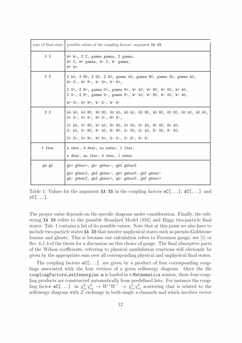
type of final state possible values of the coupling factors’ argument XA XB
V V W+ W-, Z Z, gamma gamma, Z gamma,
W+ Z, W+ gamma, W- Z, W- gamma,
W+ W+
V S Z h0, Z H0, Z G0, Z A0, gamma h0, gamma H0, gamma G0, gamma A0,
W+ G-, W+ H-, W- G+, W- H+,
Z G+, Z H+, gamma G+, gamma H+, W+ h0, W+ H0, W+ G0, W+ A0,
Z G-, Z H-, gamma G-, gamma H-, W- h0, W- H0, W- G0, W- A0,
W+ G+, W+ H+, W- G-, W- H-
S S h0 h0, h0 H0, H0 H0, G0 h0, A0 h0, G0 H0, A0 H0, G0 G0, G0 A0, A0 A0,
G+ G-, G+ H-, H+ G-, H+ H-,
G+ h0, G+ H0, H+ h0, H+ H0, G+ G0, G+ A0, H+ G0, H+ A0,
G- h0, G- H0, H- h0, H- H0, G- G0, G- A0, H- G0, H- A0,
G+ G+, G+ H+, H+ H+, G- G-, G- H-, H- H-
f fbar u ubar, d dbar, nu nubar, l lbar,
u dbar, nu lbar, d ubar, l nubar
gh gh gh+ ghbar+, gh- ghbar-, ghZ ghbarZ
gh+ ghbarZ, ghZ ghbar-, gh+ ghbarF, ghF ghbar-
gh- ghbarZ, ghZ ghbar+, gh- ghbarF, ghF ghbar+
Table 1: Values for the argument XA XB in the coupling factors eC[...], dC[...] andcC[...].
The proper value depends on the specific diagram under consideration. Finally, the sub-string XA XB refers to the possible Standard Model (SM) and Higgs two-particle finalstates. Tab. 1 contains a list of its possible values. Note that at this point we also have toinclude two-particle states XA XB that involve unphysical states such as pseudo-Goldstonebosons and ghosts. This is because our calculation refers to Feynman gauge; see [1] orSec. 6.1.3 of the thesis for a discussion on this choice of gauge. The final absorptive partsof the Wilson coefficients, referring to physical annihilation reactions will obviously begiven by the appropriate sum over all corresponding physical and unphysical final states.
The coupling factors eC[...] are given by a product of four corresponding coup-lings associated with the four vertices of a given selfenergy diagram. Once the filecouplingFactors selfenergies.m is loaded in a Mathematica session, these four-coup-ling products are constructed automatically from predefined lists. For instance the coup-ling factor eC[...] in χ0
e1χ0e2
→ W+W− → χ0e4χ0e3
scattering that is related to theselfenergy diagram with Z exchange in both single s-channels and which involves vector
12
couplings of the external χ0e1χ0e2
and χ0e4χ0e3
pairs, is then given by
eC["rr", "chi0 chi0 -> (Z) -> W+ W- -> (Z) -> chi0 chi0", 1]
= cW2 v0Z[e1,e2] v0Z[e3,e4] = cW2 v0Z[e1,e2] v0Z[e4,e3]∗ . (8)
Here cW denotes the cosine of the electroweak mixing angle.4 The factors v0Z[e1,e2]and v0Z[e3,e4] denote the vector couplings of the external neutralino pairs χ0
e1χ0e2
andχ0e4χ0e3
to the intermediate Z boson, respectively. They are kept as symbolic expressionsas long as their arguments ei with i = 1,...,4 are not set to integer values and if noslha MSSM spectrum card is read in. Only for integer-valued arguments these couplingsare later expressed in terms of mixing matrix entries and angles. The definition ofv0Z[i,j] agrees with the definition of v
(0,Z)ij given in Appendix A of [1] and Appendix
A.1 of the thesis. In the numeric code the definition of v0Z[i,j] in terms of mixingmatrices and angles is given at the end of the couplingFactors boxes.m file, wherealso all other relevant coupling factors involving the external χei states are given. As in
case of v0Z[i,j] and v(0,Z)ij , their nomenclature derives directly from the nomenclature
of the couplings in [1], Appendix A or the thesis, Appendix A.1. Further definitions ofcoupling factors that refer to interactions of the final state pair XAXB with the s-channelexchanged states can be found at the end of the file couplingFactors selfenergies.m.
In order to work with the numerical code it is, in principle, sufficient to have athand the final coupling factor expressions as given in the example above. Let usnevertheless say a few words on the internal determination of these expressions: ThecouplingFactors selfenergies.m file contains predefined lists that contain, for eachpossible selfenergy diagram, the occurring coupling factors. The list related to the aboveexample, for instance, reads
listSelfenergy["chi0 chi0 -> (Z) -> W+ W- -> (Z) -> chi0 chi0",1]
= v0Z[e1,e2], a0Z[e1,e2],v0Z[e3,e4], a0Z[e3,e4],cWWZ,cWWZ; (9)
The factor cWWZ is a place-holder for the vertex factor related to the three-point interac-tion of the two W -bosons and the Z. It is assigned to the proper vertex factor at the endof couplingFactors selfenergies.m. In order to obtain the eC[...] expressions fromlists such as the one written above, an element from each sub-list has to be chosen andmultiplied with the chosen elements from the three other sub-lists. This is automatisedwith the help of two simple functions,
GenerateSelfenergyCouplingFactors[...],
GenerateSelfenergyCouplingFactorsffbar[...], (10)
which can be found in the file couplingFactors selfenergies.m. The procedure issimilar to the coupling factor construction described in [1], Appendix A.2 and the thesis,
4At this stage in the code the experimental value is not yet assigned to cW; this will only happen ifan slha-formatted MSSM spectrum file is read in a Mathematica session. We come back to this pointof assigning numerical values to the parameters in later sections.
13
Appendix A.1.1. However let us stress that the generic reference processes used todetermine kinematic and coupling factors that are used in the numerical code differ fromthose presented in [1, 2] and in the thesis. For that reason there can be sign differencesbetween the kinematic and coupling factors derived in [1, 2] and the thesis and thecorresponding expressions used in the code.
3.2.2 Triangle diagrams
Coupling factors related to triangle amplitudes generically read
dC[n, "chi chi -> (X) -> XA XB -> chi chi", alpha] , (11)
where the arguments n and alpha can take the same values as the corresponding ar-guments of the kinematic factors kD[...] described in Sec. 3.1 and Sec. 3.1.2. Thesub-strings in the additional argument "chi chi -> (X) -> XA XB -> chi chi" referto the actual particle species involved in the triangle diagram under consideration. Asnoted in Sec. 3.2.1 the sub-string chi can take the values
chi = chi0, chi+, chi- .
The place-holder X in the argument "chi chi -> (X) -> XA XB -> chi chi" of thecoupling factors dC[...] refers to the specific s-channel exchanged particle and thereforecan take the values
X = gamma, Z, W+, W-, h0, H0, G0, A0, H+, H-, G+, G- .
The possible values for the place-holder XA XB referring to the final state particles in aneutralino/chargino pair-annihilation reaction have been collected in Tab. 1.
Similar to the case of the coupling factors eC[...] related to selfenergy diagrams,the coupling factors dC[...] are automatically constructed from predefined lists oncethe file couplingFactors triangles.m is loaded in Mathematica. For example, thecoupling factor with n = "rr r" related to the triangle diagram with alpha = 1 andsingle s-channel Z exchange in the reaction χ0
e1χ0e1
→ W+W− → χ0e1χ0e1
is then given by
dC["rr r", "chi0 chi0 -> (Z) -> W+ W- -> chi0 chi0", 1]
= cW v0Z[e1,e2] v0Z[e4,e3]∗ vW[e2,i1]∗ . (12)
While the labels ei refer to the external χ0ei
states, the label i1 is related to the χ+i1
states that can be exchanged in the t-channel of the triangle diagram. The predefinedlist from which the above expression is obtained reads
listTriangle["chi0 chi0 -> (Z) -> W+ W- -> chi0 chi0",1]
= vW[e1,i1], aW[e1,i1],CC[vW[e2,i1]], CC[aW[e2,i1]],v0Z[e3,e4], a0Z[e3,e4],cWWZ , (13)
and the function that builds the corresponding factors dC[...] from this list is named
GenerateTriangleCouplingFactors[...]. (14)
It can be found as well in the corresponding file couplingFactors triangles.m.
14

3.2.3 Box diagrams
The form of coupling factors associated with box diagrams is given by
cC[n, "chi chi -> XA XB -> chi chi", alpha] . (15)
Similar to the case of selfenergy and triangle diagrams described in the preceeding sec-tions, the arguments n and alpha in the coupling factors cC[...] take the same values asthe corresponding kinematic factors kC[...] discussed in Sec. 3.1 and Sec. 3.1.3. Again,the sub-strings chi in the additional argument "chi chi -> XA XB -> chi chi" ofcC[...] take the values
chi = chi0, chi+, chi- .
The possible values of the sub-string XA XB are collected in Tab. 1.When the file couplingFactors boxes.m is loaded all relevant cC[...] factors are
generated with the help of the function
GenerateBoxCouplingFactors[...] (16)
from predefined lists, such as for example
listBox["chi0 chi0 -> W+ W- -> chi0 chi0",1]
= vW[e1,i1], aW[e1,i1], CC[vW[e2,i1]], CC[aW[e2,i1]],CC[vW[e3,i2]], CC[aW[e3,i2]], vW[e4,i2], aW[e4,i2] . (17)
The labels ei refer to the external states χ0ei, while labels ia with a = 1,2 are associated
with the internally exchanged chargino states χ+ia, which occur in the t-channels of the
corresponding box diagram. From the above list we obtain for example the followingcoupling factor cC[...] referring to the reaction χ0
e1χ0e2
→ W+W− → χ0e4χ0e3
that isrelated to the box diagram labelled with alpha = 1 and that refers to n = "rrrr":
cC["rrrr", "chi0 chi0 -> W+ W- -> chi0 chi0", 1]
= vW[e1,i1] vW[e2,i1]∗ vW[e3,i2]∗ vW[e4,i2] . (18)
The neutralino-chargino W± vector coupling vW[i,j] is evaluated only for integer argu-ments i,j and otherwise left as it stands above. Its definition in terms of mixing matrixentries and angles is given at the end of couplingFactors boxes.m.
3.3 Partial wave coefficients: generic routine
In this section we describe functions provided in the file partialwavecoefficients.m,which allow to determine the absorptive part of a specific partial wave coefficient in theNRMSSM. Kinematic and coupling factor expressions have to be loaded in advance inMathematica and an slha-formatted MSSM spectrum card has to be read in, before the
15
respective coefficients can be calculated.5 In Sec. 3.3.1 we first discuss the central functionPartialWaveCoefficient[...] that allows to determine the coefficients. Sec. 3.3.2then contains a summary on further auxiliary functions needed in building the partialwave coefficient expressions.
3.3.1 The function PartialWaveCoefficient[...]
The function PartialWaveCoefficient[...] allows to determine the contribution tothe absorptive part of a partial wave coefficient that is associated with a specific exclusiveχe1χe2 → XAXB → χe4χe3 reaction. Let us recall that the actual coefficient is determinedfrom the inclusive reaction. The inclusive result is obtained from a different functiondiscussed in Sec. 4.3.
PartialWaveCoefficient[...] has the following arguments
PartialWaveCoefficient[Process, p1,p2, p3,p4, pA,pB, Wave, mci]. (19)
• The first argument, Process, is given by a string that specifies the exclusive reac-tion χe1χe2 → XAXB → χe4χe3 . It has to have the same form as the strings thatappear as arguments in the coupling factors cC[...] referring to box diagrams, seeSec. 3.2.3. For example, if a partial wave coefficient associated with the reactionχ01χ
01 → W+W− → χ0
1χ01 shall be evaluated, the argument Process is given by the
string
"chi0 chi0 -> W+ W- -> chi0 chi0" .
The possible strings that are viable arguments are easily built from the genericform
"chi chi -> XA XB -> chi chi"
by using Tab. 1 to identify the possible values of XA XB and choosing the value forchi out of the set of values chi = chi0, chi+, chi- according to the exclusiveprocess χe1χe2 → XAXB → χe4χe3 under consideration.
• The arguments p1,p2,p3 and p4 refer to the particle species χe1 , χe2, χe3 and χe4
in the process. Each argument pa with a = 1,2,3,4, can take the values
pa =
Neu[i] if χea = χ0i , i = 1, . . . , 4 ,
Cha[j] if χea = χ0j , j = 1, 2 ,
and has to be adjusted according to the particle species χea in the reaction. In theabove example of χ0
1χ01 → W+W− → χ0
1χ01 scattering we would have to set all pa
with a=1,2,3,4 to Neu[1].
5In order to read such a MSSM spectrum card we use the same file, readLHA.m, as in the Sommerfeld-enhancement part of the code. This file contains the function ReadMSSMInput[filename], where theinput filename must be an slha formatted MSSM spectrum card. In order to adjust the nomenclatureslightly to the annihilation matrix code, one has to load the file readSUSYparameters.m after callingReadMSSMInput[filename]. In this way only certain names for masses and couplings are adjusted. Fordetails on the nomenclature we refer the reader to the self-explanatory file readSUSYparameters.m.
16
• The values of pA (pB) are given by the values of XA and XB, which can be read ofTab. 1, where however all signs have to be dropped. In our exclusive scatteringreaction example χ0
1χ01 → W+W− → χ0
1χ01 , for instance, pa and pB have to be set
to pA = pB = W.
• The possible inputs for Wave specify the partial wave configuration and agree withthose specified under 2s+1LJ in Sec. 3.1.
• The possible values for mci are mci = mc1,mc2 and indicate the underlying expan-sion in mass differences, see the corresponding paragraph in Sec. 3.1.
To summarise, we obtain in our χ01χ
01 → W+W− → χ0
1χ01 exclusive process example from
PartialWaveCoefficient["chi0 chi0 -> W+ W- -> chi0 chi0",
Neu[1],Neu[1],Neu[1],Neu[1],W,W,mc2,"1S0,p2"]
the contribution to the next-to-next-to-leading order 1S0 Wilson coefficient associatedwith χ0
1χ0 → W+W− → χ0
1χ01 scattering. This corresponds to the next-to-next-to-
leading order 1S0-wave contribution to the χ01χ
01 → W+W− annihilation cross section.
As a side remark let us recall that in case of identical particle annihilation χe1 = χe2 andfurther χe1χe2 = χe4χe3 the choice of either mass expansion option mc1 or mc2 gives thesame result for the coefficient, see [1, 2] or Sec. 5 and 6 in the thesis.
The absorptive part of any Wilson coefficient of a NRMSSM four fermion operatoris obtained from the sum of contributions related to box, triangle and selfenergy dia-grams. Accordingly, the function PartialWaveCoefficient[...] calls three individualfunctions that have the same arguments as the former and that separately evaluate thecontributions from box, triangle and selfenergy diagrams. These functions are named
BoxCoefficient[Process, p1,p2, p3,p4, pA, pB, Wave, mci], (20)
TriangleCoefficient[Process, p1,p2, p3,p4, pA, pB, Wave, mci], (21)
SelfCoefficient[Process, p1,p2, p3,p4, pA, pB, Wave, mci]. (22)
The type of diagrams that appear in case of a final state fermion pair XAXB = ff differsslightly from the case of final states built from gauge or Higgs bosons. In particular, ascan be inferred from Sec. 3.1 and Sec. 3.2, the number of kinematic and coupling factorexpression is larger for XAXB = ff . Therefore there is a separate function
PartialWaveCoefficientFermions[...], (23)
that covers the case of reactions where XAXB = ff and which, in addition to theunchanged function BoxCoefficient[...], calls
TriangleCoefficientFermions[...] , (24)
SelfCoefficientFermions[...]. (25)
17
The arguments of the above functions are as in PartialWaveCoefficient[...]. How-ever, there is one subtlety regarding the nomenclature of fermion final state parameterspA,pB:
uQuark[I] denotes the up-type quark of the Ith family, uI ,
dQuark[I] denotes the down-type quark of the Ith family, dI ,
neutrino[I] denotes the neutrino of the Ith family, νI ,
lepton[I] denotes the lepton of the Ith family, lI . (26)
For example, in case of the reaction χ01χ
+1 → tb → χ+
1 χ01 the values of pa,pB inside the
above functions have to be set to pA = uQuark[3] and pB = dQuark[3].
3.3.2 Auxiliary functions in partialwavecoefficients.m
In order to determine the exclusive final state contribution of a certain partial wavecoefficient with the function PartialWaveCoefficient[...], the terms in the generickinematic factors and the coupling factor expressions have to be set to numerical values.To this end a slha-formatted MSSM spectrum card has to be read in the Mathematica
session. Once the MSSM spectrum is read in, all values for the masses, angles and mixingmatrices are available and only have to be assigned according to the χe1χe2 → XAXB →χe4χe3 reaction under consideration.
For each exclusive scattering reaction we can generically distinguish between the setof external particles and the internally exchanged (virtual) states. The former set ofstates contains the χei , i = 1, . . . , 4 species as well as the on-shell accessible final statesXA, XB. The function PartialWaveCoefficient[...] calls the subroutine
SetExternalVar[p1, p2, p3, p4, pA, pB, mci]. (27)
This function assigns numerical values to the process specific external mass parametersM,m,m and δm, δm (denoted by M,m,mbar and dm, dmbar in the numerical code) aswell as mA, mB (given by mA,mB in the program). Let us recall from [1, 2] and from thethesis that the mass parameters M,m,m depend on the choice of the mass expansionoption, mci, where
m =1
2(me1 +me3) , m =
1
2(me2 +me4) for mci = mc1,
m =1
2(me1 +me4) , m =
1
2(me2 +me3) for mci = mc2,
(28)
and similarly also for δm and δm. Further, SetExternalVar[..] also extracts the labelsei of the external χei states that refer to a specific neutralino or chargino species. Forinstance, if the argument p1 of the SetExternalVar function is Neu[1], the value of e1is set to e1 = 1. Note that the argument e1 is the same as the one appearing in thecoupling factors.6
6As noted in Sec. 3.2 the coupling factors cC[...], dC[...] and eC[...] can be assigned numericalvalues only if all the arguments ea with a=1,2,3,4 and ib with b=1,2 (indices ib refer to the internallyexchanged particle states) related to the individual couplings at each vertex are set to integer values.
18
While the parameters related to the external states χei and XA, XB can be assignedonce and for all their corresponding numerical values, the case of the intermediate statesis more involved as typically a summation over several internally exchanged states in eachdiagram has to be taken into account. For instance, in the four box diagrams labelledwith α = 1, . . . , 4 and related to χ0
1χ01 → W+W− → χ0
1χ01, in each of the two t-channels
both chargino species χ+j , j = 1, 2 can be exchanged. Consequently, each of the box
topologies α in this case actually represents four different diagrams: the intermediatelyexchanged chargino species can be given by χ+
1 χ+1 , χ
+1 χ
+2 , χ
+2 χ
+1 and χ+
2 χ+2 where the
first (second) element in each tuple refers to the chargino species exchanged in the left(right) t-channel. In each case the masses of the t-channel exchanged species and theircorresponding label have to be set accordingly in order to determine the numerical valueof the kinematic and coupling factor expressions. This is taken care of by a Do[]-loop inPartialWaveCoefficient[...], which calls elements from predefined lists containingall possible tuples of internally exchanged particles related to each of the diagrams inFig. 1–3.
At this stage the only missing point before a numerical value for a specific partialwave coefficient can be given is the introduction of predefined lists that, for each possibleprocess, contain the information on the internally exchanged particle species. We discussthe structure of these lists in the next section.
3.4 Partial wave coefficients: physical reactions
3.4.1 Listing internally exchanged states
When the function PartialWaveCoefficient[...] is called for a specific exclusivereaction, it accesses predefined lists collected in the files scatteringchannels box.m,scatteringchannels triangles.m and scatteringchannels self.m, which summa-rise the relevant information on the internally exchanged particles in each contributingdiagram. Each of the latter scatteringchannels xxx.m files generically contains twotypes of lists. In the following we discuss their form for each of the three relevanttopologies in turn.
The file scatteringchannels box.m summarises the following two types of lists:
BoxSubProcess[Process],
tChannelBox[Process, alpha].(29)
In both cases the argument Process specifies the exclusive reaction under consideration.Accordingly, it takes the same values as in the function PartialWaveCoefficient[...],see Sec. 3.3. The argument alpha refers to the label of the box diagram according toour counting scheme, see Fig. 3 and Sec. 3.1 and 3.2. For each possible χe1χe2 →XAXB → χe4χe3 process BoxSubProcess[Process] is given by a hard-coded list withtwo elements. The purpose of the list is to provide the arguments for the couplingand kinematic factors that have to be multiplied with each other, respectively, whenbuilding the Wilson coefficients. Consequently, the form of the two elements of each
19
list is dictated by the nomenclature that we have chosen for the kinematic and couplingfactor expressions: The first element is given by the process-specifying string that occursin the coupling factor expressions related to the reaction, while the second element isthe string arising as argument in the corresponding kinematic factor term. In case of allprocesses χ0
e1χ0e2
→ W+W− → χ0e4χ0e3, irrespective which neutralino species with labels
ei are involved, we have, for instance,
BoxSubProcess["chi0 chi0 -> W+ W- -> chi0 chi0"]
= "chi0 chi0 -> W+ W- -> chi0 chi0", "chi chi -> V V -> chi chi". (30)
The elements of the lists tChannelBox[...] are given by sublists with two elements,where the first (second) element gives the particle species exchanged in the left (right)t-channel of a contributing box amplitude with label alpha. In our χ0
e1χ0e2→ W+W− →
χ0e4χ0e3
example – for all the box diagrams with labels α = 1, 2, 3, 4 – the t-channelexchanged species are given by the two chargino species χ+
1,2. Consequently the corre-sponding tChannelBox[...] list reads, for all alpha=1,2,3,4,
tChannelBox["chi0 chi0 -> W+ W- -> chi0 chi0", alpha]
= Cha[1],Cha[1],Cha[1],Cha[2],Cha[2],Cha[1],Cha[2],Cha[2] . (31)
The lists provided in scatteringchannels triangles.m are named
TriangleSubProcess[Process],
tsChannelTriangles[SubProcess, alpha],(32)
and have a similar form as the lists related to box diagrams described above. Thepossible arguments Process of the expressions TriangleSubProcess[...] are identicalto the arguments of BoxSubProcess[...]. The lists that are obtained when calling aspecific TriangleSubProcess[Process] are built from several sub-lists, where each ofthe latter contains as first element a sub-process specifying string occurring as element ofa corresponding coupling factor expression. The respective second argument is the stringcorresponding to the related kinematic factor. Under a “sub-process specifying string”we understand a string that explicitly contains the s-channel exchanged particle species.For triangle diagrams in the example scattering process χ0
e1χ0e2
→ W+W− → χ0e4χ0e3
wehave
TriangleSubProcesses["chi0 chi0 -> W+ W- -> chi0 chi0"]
= "chi0 chi0 -> (H0) -> W+ W- -> chi0 chi0",
"chi chi -> (S) -> V V -> chi chi","chi0 chi0 -> (h0) -> W+ W- -> chi0 chi0",
"chi chi -> (S) -> V V -> chi chi","chi0 chi0 -> (Z) -> W+ W- -> chi0 chi0",
20
"chi chi -> (V) -> V V -> chi chi". (33)
The argument SubProcess in a list tsChannelTriangle[SubProcess, alpha] can takethe values provided by the first elements of the sub-lists in TriangleSubProcess[...].The corresponding tsChannelTriangle[...] lists contain sub-lists where the first (sec-ond) element gives a particle exchanged in the t-channel (s-channel) of the correspondingtriangle diagram with label alpha. Again, for our explicit χ0
e1χ0e2
→ W+W− → χ0e4χ0e3
example we have for all alpha=1,2,3,4,
tsChannelTriangle["chi0 chi0 -> (H0) -> W+ W- -> chi0 chi0", alpha]
= Cha[1], H0, Cha[2], H0. (34)
According to the sub-lists in the corresponding TriangleSubProcess[...] for our ex-ample there are in addition two further tsChannelTriangle[...], where the s-channelexchanged state is given by a h0 or a Z boson.
The structure of the lists contained in scatteringchannels self.m follows immediatelyfrom the above discussed cases. Here the nomenclature for the lists is
SelfSubProcesses[Process],
ssChannelSelf[SubProcess].(35)
The argument Process of the first type of lists takes the same values as in the corre-sponding box and triangle diagram related cases: Process is a place-holder for a stringspecifying the exclusive χe1χe2 → XAXB → χe4χe3 scattering reaction. The elements ofa certain SelfSubProcesses[Process] list are again sub-lists that contain as elementsthe process specifying strings related to coupling and corresponding kinematic factors.For instance we have
SelfSubProcesses["chi0 chi0 -> W+ W- -> chi0 chi0"]
= "chi0 chi0 -> (Z) -> W+ W- -> (Z) -> chi0 chi0",
"chi chi -> (V) -> V V -> (V) -> chi chi", 1,"chi0 chi0 -> (Z) -> W+ W- -> (H0) -> chi0 chi0",
"chi chi -> (V) -> V V -> (S) -> chi chi", 2,..., ... . (36)
The enumeration index that occurs as third element of the sub-lists is the label alpharelated to selfenergy topologies which we introduced in Sec. 3.1.1. The possible ar-guments of ssChannelSelf[...] are now given by the respective first sub-elementsof SelfSubProcess[...], and the latter lists contain as elements pairs i1,i2 of allpossible s-channel exchanged particles i1,i2. For instance
ssChannelSelf["chi0 chi0 -> (Z) -> W+ W- -> (Z) -> chi0 chi0"] = Z, Z,ssChannelSelf["chi0 chi0 -> (Z) -> W+ W- -> (H0) -> chi0 chi0"] = Z, H0,
21
... , (37)
where we do not write explicitly the remaining seven lists related to the selfenergytopology in χ0
e1χ0e1
→ W+W− → χ0e4χ0e3
scattering.
3.4.2 The function pwc[...] related to the physical exclusive process
We have noted before in Sec. 3.3 that the function PartialWaveCoefficient[...] de-termines the contribution to the absorptive part of a Wilson coefficient that arises froma specific exclusive XAXB final state.7 As our calculation refers to Feynman gauge, wehave to sum over a certain set of final states XAXB to arrive at corresponding con-tributions from physical final states. In order to immediately have at hand a func-tion that gives the exclusive physical final state contribution to the Wilson coefficients,the function pwc[...] (abbreviating partialwavecoefficient) is introduced in the filepartialwavecoefficients channels.m. It has the form
pwc[Process, e1,e2, e3,e4, Wave, mci], (38)
where the arguments can take the following values:
• Process is a string indicating the exclusive physical reaction
"chi chi -> XA XB -> chi chi"
where all sub-strings chi and XA XB have to be adjusted according to the exclusivereaction under consideration. Note in particular, that the generic species of theexternal states (neutralino, chi0, or chargino, chi+, chi-) is fixed by this string.
• e1, e2, e3, e4 denote the labels ei of the external states χei in the physicalχe1χe2 → XAXB → χe4χe3 reaction.8 As the particle species type of each χei,either being a neutralino or a chargino, is already determined by the argumentProcess, only the labels ei need to be specified as additional inputs here.
7Let us recall in addition from Sec. 3.3 that in case of an exclusive final state built of a fermion pairthe corresponding function is named PartialWaveCoefficientFermions[...].
8A caveat has to be added here, related to the use of the functions pwc[...]: These functionscurrently contain no internal query if a given final state XAXB is on-shell accessible in χe1χe2 → XAXB
and χe4χe3 → XAXB reactions. However an absorptive part is only present in χe1χe2 → XAXB →χe4χe3 scattering, if XA and XB can simultaneously go on-shell. Consequently, the result for a pwc[...]should be zero, if the state XAXB cannot be produced on-shell in the corresponding χe1χe2 → XAXB
and χe4χe3 → XAXB annihilations. But when calling pwc[...], the hard coded analytic results for theunderlying kinematic factors are called, which rely on a calculation under the assumption that XAXB
can be produced on-shell. Therefore, in the current version of the code, the user himself has to makesure that XAXB is on-shell accessible when using pwc[..] and if XAXB is not on-shell accessible hehas to set the result for the exclusive contribution to the partial wave coefficient to zero by hand. Letus note that in the case of the determination of the inclusive reactions, referring to the absorptive partsof the Wilson coefficients, described in Sec. 4.3 it is taken care of that only those XAXB exclusive finalstate contributions are considered that are on-shell accessible.
22
• Wave takes the same values as in the function PartialWaveCoefficient[...], seeSec. 3.3 and Sec. 3.1 for the possible values.
• mci can be either set to mc1 or mc2, specifying the mass expansion option, seeagain Sec. 3.3 and Sec. 3.1.
Let us imagine we wish to determine the contribution to the leading order 3S1 partialwave coefficient in χ0
1χ02 → χ0
1χ02 scattering that arises from a physical W+W− exclusive
final state, and we chose the mass expansion mc2. In this case we have to call
pwc["chi0 chi0 -> W+ W- -> chi0 chi0", 1, 2,2, 1, "3S1", mc2]. (39)
Note the order in which the indices ei of the external states χei are given: accordingto ascending i, while we denote the scattering reaction itself by χe1χe2 → χe4χe3. Thatis, the indices of the particles with labels e3 and e4 appear in the opposite order. Thisnomenclature goes back to the conventions that we have chosen for the order of indiceson the four-fermion operators in [1, 2] and in the thesis. It implies, in particular, that acertain partial wave contribution to the exclusive pair annihilation cross section of twonon-identical states χe1χe2 , which is related to the absorptive part in χe1χe2 → χe1χe2
scattering, is obtain from pwc[...] by setting the arguments e1,e2,e3,e4 toe1,e2,e2,e1. Therefore the output of our above example is proportional to theleading order 3S1 wave contribution to the exclusive χ0
1χ02 → W+W− annihilation cross
section.The file scatteringchannels channels.m contains the definition of all functions
pwc[Process, ...] with differing arguments Process that are related to possible ex-clusive physical χe1χe2 → XAXB → χe4χe3 reactions arising in neutralino and charginoscattering reactions. In case of fermionic final states XAXB the colour factor of Nc = 3is taken into account in the definition of the corresponding pwc[...].
4 Part 2: Building the annihilation matrices
In this section we describe the functions that finally allow to obtain the annihilationmatrices encoding hard χe1χe2 →
∑
XAXB → χe4χe3 pair-annihilation reactions. Theseannihilation matrices are an input to the Sommerfeld enhancement part of the code.Collecting and representing the hard χe1χe2 →
∑
XAXB → χe4χe3 rates in matrixform requires the introduction of an enumeration convention for the χeaχeb two-particlestates. Sec. 4.1 summarises our enumeration convention for the two-particle states χeaχeb
in each of the charge sectors referring to neutral, single- or double-charged χeaχeb pairs.In Sec. 4.2 we comment on the choice to be made for the mass expansion option, eithermc1 or mc2. While in the first part of the code, discussed in Sec. 3, we have describedfunctions that allow to obtain partial wave separated contributions to the NRMSSMfour-fermion operators arising from exclusive (physical) final states, we finally introducein Sec. 4.3 functions that determine the full absorptive part of the Wilson coefficientsrelated to inclusive reactions. Symmetry factors and symmetry relations between certain
23

(χχ)I state method-1 label method-2 label (χχ)I state method-1 label method-2 label
χ+1 χ
+1 1 1 χ+
2 χ+1 3 -
χ+1 χ
+2 2 2 χ+
2 χ+2 4 3
Table 2: Enumeration scheme within method-1 and method-2 for double positive charged(χχ)I states. The same conventions hold for double negative charged states.
partial wave coefficients are discussed in Sec. 4.4. Compared to the order of magnitudeof leading entries in the annihilation matrices, certain entries can be numerically verysmall and can be set to zero for our purposes; a corresponding function that addressesthis issue is discussed in Sec. 4.5. The functions that determine the annihilation matricesare finally given in Sec. 4.6
It is worth to note here that all functions described in the following are introduced anddefined in the file annihilationmatrices vx.m, where x denotes the version number,which is currently x=7.
4.1 Enumeration convention for χχ states
The entries of the annihilation matrices encode the absorptive part of partial wave sep-arated χe1χe2 → χe4χe3 scattering reactions. As they refer to two-particle scatteringswe can first divide all possible pairs built from the neutralino and chargino states intosets of neutral, single positive (single negative) and double positive (double negative)χχ states. In the following we will consider χeaχeb pairs rather than individual χea andχeb states and therefore introduce a single label I to refer to the pair χeaχeb ≡ (χχ)I .Let us note that we generically consider all possible χχ pairs as external states in theannihilation matrices. This implies that not only those (χχ)I pairs built from NRMSSMstates are considered, but also those (χχ)K pairs that are too heavy to be part of theNRMSSM. As described in [3] as well as in Sec. 8.6 of the thesis, the effect of heavy χχstates – not being part of the NRMSSM set of χχ states – is taken into account in thelast loop prior to the hard annihilation reaction in the ladder-diagrams accounting forthe Sommerfeld enhancement effect. One input in the corresponding calculation are theperturbative hard annihilation rates involving the heavy χχ states. Therefore also theserates are determined in the annihilation matrix part of the code.
Within a given charge sector – neutral, single positive (single negative) or doublepositive (double negative) – the IJ entry of an annihilation matrix ΓIJ encodes the ab-sorptive part of the inclusive (χχ)J → (χχ)I scattering reaction. Note the order of statesin the reaction: the columns (rows) of Γ contain all processes with one fixed incoming(outgoing) state. In each charge sector the Jth column (Ith row) of the annihilationmatrices Γ refers to the incoming (outgoing) two-particle state with enumeration labelJ (I) according to the enumeration convention of the states summarised in Tabs. 2–4.Note that this enumeration convention obviously has to agree with the one set up inthe ”Sommerfeld-enhancement part” of the code. Further recall from [3] or Sec. 8.3 of
24
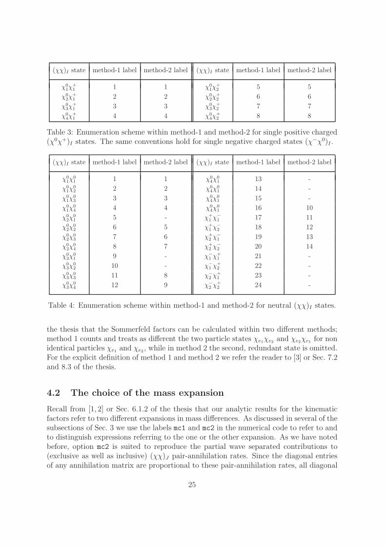
(χχ)I state method-1 label method-2 label (χχ)I state method-1 label method-2 label
χ01χ
+1 1 1 χ0
1χ+2 5 5
χ02χ
+1 2 2 χ0
2χ+2 6 6
χ03χ
+1 3 3 χ0
3χ+2 7 7
χ04χ
+1 4 4 χ0
4χ+2 8 8
Table 3: Enumeration scheme within method-1 and method-2 for single positive charged(χ0χ+)I states. The same conventions hold for single negative charged states (χ−χ0)I .
(χχ)I state method-1 label method-2 label (χχ)I state method-1 label method-2 label
χ01χ
01 1 1 χ0
4χ01 13 -
χ01χ
02 2 2 χ0
4χ01 14 -
χ01χ
03 3 3 χ0
4χ01 15 -
χ01χ
04 4 4 χ0
4χ01 16 10
χ02χ
01 5 - χ+
1 χ−1 17 11
χ02χ
02 6 5 χ+
1 χ−2 18 12
χ02χ
03 7 6 χ+
2 χ−1 19 13
χ02χ
04 8 7 χ+
2 χ−2 20 14
χ03χ
01 9 - χ−
1 χ+1 21 -
χ03χ
02 10 - χ−
1 χ+2 22 -
χ03χ
03 11 8 χ−
2 χ+1 23 -
χ03χ
04 12 9 χ−
2 χ+2 24 -
Table 4: Enumeration scheme within method-1 and method-2 for neutral (χχ)I states.
the thesis that the Sommerfeld factors can be calculated within two different methods;method 1 counts and treats as different the two particle states χe1χe2 and χe2χe1 for nonidentical particles χe1 and χe2, while in method 2 the second, redundant state is omitted.For the explicit definition of method 1 and method 2 we refer the reader to [3] or Sec. 7.2and 8.3 of the thesis.
4.2 The choice of the mass expansion
Recall from [1, 2] or Sec. 6.1.2 of the thesis that our analytic results for the kinematicfactors refer to two different expansions in mass differences. As discussed in several of thesubsections of Sec. 3 we use the labels mc1 and mc2 in the numerical code to refer to andto distinguish expressions referring to the one or the other expansion. As we have notedbefore, option mc2 is suited to reproduce the partial wave separated contributions to(exclusive as well as inclusive) (χχ)J pair-annihilation rates. Since the diagonal entriesof any annihilation matrix are proportional to these pair-annihilation rates, all diagonal
25
entries of the annihilation matrices rely on a calculation using mc2 kinematic factors.However, in case of off-diagonal annihilation matrix entries referring to reactions
(χχ)J → (χχ)I with J 6= I it is a priori not clear whether mc1 or mc2 expressions shouldbe chosen in the calculation. Generically the mass differences δm, δm should be smallfor the mass expansion to be consistent, see the discussion in [1] or Sec. 6.1.2 of thethesis. In order to decide which expansion mci should be chosen in the evaluation ofoff-diagonal entries ΓJI in the code we introduce functions that address this questionbased on the given MSSM neutralino and chargino mass spectrum. These functions, incase of neutral χe1χe2 → χe4χe3 two-particle state scatterings, are named
Mcinnnn[e1,e2,e3,e4] for χ0e1χ0e2→ χ0
e4χ0e3
reactions,
Mcinncc[e1,e2,e3,e4] for χ0e1χ0e2→ χ−
e4χ+e3
reactions,
Mciccnn[e1,e2,e3,e4] for χ−e1χ+e2→ χ0
e4χ0e3
reactions,
Mcicccc[e1,e2,e3,e4] for χ−e1χ+e2→ χ−
e4χ+e3
reactions,
(40)
while in single charged reactions the corresponding functions are named
Mcinccn[e1,e2,e3,e4] for χ0e1χ+e2→ χ0
e4χ+e3
reactions,
Mcicnnc[e1,e2,e3,e4] for χ−e1χ0e2→ χ−
e4χ0e3
reactions.(41)
In case of double charged reactions the function Mcicccc[e1,e2,e3,e4] introduced in(40) can be used. The four arguments ei, i=1,2,3,4 of all these functions are the labelsof the external χei states, respectively. The reason why so many different functions areintroduced is related to these arguments: if we have only the information on the labelbut have to deal with particle masses, we need an additional information on the involvedparticle species (neutralino or chargino).
The output of all functions given in (40) and (41) is either mc1 or mc2. Which outputis returned should be related to the value of the mass differences δm, δm calculated forboth expansion options mc1 and mc2, respectively, given a specific underlying MSSMspectrum; the mass expansion mci where the mass differences are smaller should bechosen. This is because the smaller the mass differences the better the convergence ofthe expansion of the perturbative χχ → XAXB → χχ rates in mass differences δmand δm. The currently implemented criterion reads as follows: if particle χe1 is lighter(heavier) than χe2 and at the same time particle χe4 is lighter (heavier) than χe3 , thenoption mc2 is chosen and the output of the corresponding functions in (40) and (41) ismc2. Otherwise the output of the above function is set to mc1.
The Mcixxxx[...] functions will appear inside some of the functions described inthe following that determine the full partial wave coefficients.
4.3 Inclusive reactions: the final partial wave coefficients
In order to build the full partial wave coefficients referring to inclusive reactions fromtheir respective exclusive XAXB final state contributions9 we have to decide – based
9Recall that the functions pwc[...] providing the contributions to the absorptive parts of the Wilsoncoefficients from exclusive (tree-level) reactions χe1χe2 → XAXB → χe4χe3 are described in Sec. 3.4.2.
26
on the given MSSM spectrum – which XAXB final states are on-shell accessible in aχeaχeb → XAXB annihilation reaction. Obviously, the heavier the states χea and χeb themore final states XAXB will be accessible on-shell. However, our currently implementedcriterion to tread a XAXB state as viable final state in a χeaχeb → XAXB annihilationreaction related to χe1χe2 → XAXB → χe4χe3 scattering – and hence our criterion to takeinto account an exclusive final state in the construction of the annihilation matrices – isbased on the lightest two-particle state χ0
1χ01. The reason for this is related to the Som-
merfeld enhancements that shall eventually be calculated using the annihilation matrixresults provided by the code, and reads as follows: Off-diagonal potential scattering canconvert an incoming χ0
1χ01 pair to another neutral χeaχeb state that eventually undergoes
pair annihilation. The latter annihilation reaction is encoded in the annihilation matri-ces. Therefore we have to take care that in Sommerfeld enhanced reactions with initiallyincoming χ0
1χ01 states only those XAXB final states are considered in the inclusive partial
wave coefficients, encoded in the annihilation matrices, that are accessible for the χ01χ
01
pair. Our criterion is therefore such, that all XAXB final states that cannot be producedon-shell in χ0
1χ01 → XAXB processes are excluded as exclusive final states for any par-
tial wave coefficient. Even more, in our NRMSSM effective theory set-up, the on-shellaccessible final state particles XAXB should not be non-relativistic, otherwise we wouldhave to consider them among the set of non-relativistic states of the theory and even co-annihilation rates of such additional non-relativistic states could be relevant. Thereforewe establish the following criterion to account for a XAXB final state in the numericalcode: If the sum of masses mA + mB is smaller than half the mass of the χ0
1χ01 pair a
corresponding flag is set to 1 in the code, otherwise the flag is set to 0. The full partialwave coefficients are obtained from the sum over all XAXB state contributions, whereeach contribution is multiplied by the corresponding flag. Consequently only those finalstate contributions are taken into account for the full partial wave coefficient that fulfillthe above stated criterion related to the χ0
1χ01 mass. Note that the flags are introduced
in the file annihilationmatrices vx.m as well.The following functions determine the absorptive parts of the full partial-wave coeffi-
cients related to χe1χe2 → χe4χe3 scattering, taking only those exclusive XAXB final statecontributions into account that are on-shell accessible in χ0
1χ01 → XAXB annihilations:
pwcFullnnnnALT[e1,e2,e4,e3, Wave, mci] for χ0χ0 → χ0χ0 reactions,
pwcFullccccALT[e1,e2,e4,e3, Wave, mci] for χ−χ+ → χ−χ+ reactions,
pwcFullnnccALT[e1,e2,e4,e3, Wave, mci] for χ0χ0 → χ−χ+ reactions, (42)
are the functions relevant for neutral scattering reactions. The absorptive parts of theWilson coefficients in off-diagonal χ−χ+ → χ0χ0 scattering can be obtained from thecorresponding χ0χ0 → χ−χ+ expressions. Note the order of arguments e4 and e3 thatnow appear in the same order as in χe1χe2 → χe4χe3. The values that all the argumentsof the pwcFullxxxxALT[...] functions can take should be obvious from the preceedingsections. In case of single charged reactions we have the corresponding functions
pwcFullnccn[e1,e2,e4,e3, Wave, mci] for χ0χ+ → χ0χ+ reactions,
27
pwcFullcnnc[e1,e2,e4,e3, Wave, mci] for χ−χ0 → χ−χ0 reactions. (43)
Finally, for double charged reactions the corresponding full partial wave coefficients areobtained with functions
pwcFullcpcpALT[e1,e2,e4,e3, Wave, mci] for χ+χ+ → χ+χ+ reactions,
pwcFullcmcmALT[e1,e2,e4,e3, Wave, mci] for χ−χ− → χ−χ− reactions. (44)
Note that mci appears as an argument of all the above functions. There is a versionpwcFullxxxx[...] of these function – in case of neural and double-charged reactionswithout the ending ALT10 – where the appropriate mci value to be used in the calculationof a partial wave coefficient is internally determined inside the function with the help ofthe Mcixxxx[...] functions described in Sec. 4.2.
4.4 Symmetry factors and symmetry relations
Certain entries of the annihilation matrices have to refer to reactions χ+χ− → χ0χ0
instead of χ−χ+ → χ0χ0 and to χ0χ0 → χ+χ− instead of χ0χ0 → χ−χ+. Similarlythere are entries related to χ−χ+ → χ+χ−, χ+χ− → χ−χ+ or χ+χ− → χ+χ− scatteringinstead of χ−χ+ → χ−χ+. The respective Wilson coefficients that are not determinedby the functions given in Sec. 4.3 can be obtained from the latter by making use ofcertain symmetry properties of the Wilson coefficients under exchange of labels. For thecorresponding relations see for instance eq. (8) in [1] or eq. (5.9) and eq. (5.14) in thethesis.
In the code we introduce the parameter SymFac[Wave] that, depending on the argu-ment Wave, is either given by 1 or −1 and that agrees with the parameter η in eq. (9)of [1] and eq. (5.10) in the thesis. This allows to finally introduce the following functions
pwcFullnnmpALT[e1,e2,e3,e4, Wave, mci] for χ0e1χ0e2→ χ+
e4χ−e3
reactions,
pwcFullpmmpALT[e1,e2,e3,e4, Wave, mci] for χ+e1χ−e2→ χ+
e4χ−e3
reactions, (45)
derived from corresponding functions pwcFullxxxxALT[...] in Sec. 4.3. For details ofthe relations to the Sec. 4.3 functions we refer the reader to the part of the code wherethe definitions of the above functions are given as well as to the relevant paragraphsin [1] or Chap. 5 of the thesis.
The annihilation matrices used in the ”Sommerfeld-enhancement part” of the codeshall already involve the spin-summed inclusive annihilation reactions. For that reasonwe further introduce certain spin-weight parameters in the code, named SpinSum[Wave].These will multiply the appropriate partial wave coefficients when building the annihila-tion matrices from the latter. In our case SpinSum[Wave] takes always the value 1 apartfrom the case of 3S1 partial wave reactions where it is given by 3.
10The ending ALT denotes “alternative” and was introduced in case of annihilation matrices relatedto neutral and double charged reactions in course of the code development.
28
4.5 Chopping numerically small annihilation matrix entries
Due to small numerical inaccuracies in the calculation of the partial wave coefficientssome of the annihilation matrix entries that should be exactly zero happen to be non-vanishing. In addition there are further entries that are non-vanishing but stronglysuppressed with respect to the leading entries.11 Within the part of the code thatdetermines the Sommerfeld enhancement factors both these types of strongly suppressedentries can potentially cause numerical problems. For that reason we introduce a functionthat sets all those annihilation matrix entries to zero that are smaller by a certain factorthan the leading entry. The relevant function is named
chopRoutineALT[Matrix, Wave]. (46)
Its first argument Matrix will in our application be an annihilation matrix and thesecond argument specifies the partial wave configuration of that annihilation matrix.The output of chopRoutineALT[Matrix, Wave] is the input Matrix where however allthose entries that are by a certain amount smaller than the leading matrix-entry are setto zero: In case of leading order S-wave related annihilation matrices those entries areset to zero that are smaller than the leading entry by a factor of 10−12. For the case ofall P - and next-to-next-to-leading order S-wave matrices the factor is chosen to be 10−8.
4.6 Calculation of the annihilation matrices
Now we have all functions available that allow to determine the annihilation matrices.Particularly relevant for the determination of the respective matrix entries are the func-tions pwcFullxxxxALT[...], pwcFullnccn[...] and pwcFullcnnc[...] discussed inSec. 4.3 that give as output the absorptive parts of the full, partial wave separated Wilsoncoefficients; apart from possible spin weight factors, the latter determine the respectiveannihilation matrix entries. Our last step is therefore the construction of the matricesΓ from their individual components ΓIJ related to (χχ)J → (χχ)I scattering. Let usrecall that our specific enumeration convention for the states (χχ)I in each charge sectoris given in Sec. 4.1, see in particular Tabs. 2–4 therein.
We provide the following functions that give as output the partial wave specificannihilation matrices in each charge sector corresponding to the method-1 enumerationconvention:12
GammaNeutralALT[Wave] for neutral χχ → χχ reactions,
11The typical order of magnitude of such numerically strongly suppressed annihilation matrix entriesis 10−25GeV−2 in case of leading order S-wave matrices while the corresponding leading entries aretypically of O(10−10 − 10−12GeV−2). In case of P - and next-to-next-to-leading order S-wave annihi-lation matrices, the corresponding numerically strongly suppressed entries are typically smaller thanO(10−25 GeV−4) while leading entries are typically of O(10−16 − 10−18GeV−4). The order of magni-tude of annihilation matrix entries obviously depends on the underlying MSSM spectrum and the abovequoted numbers are rather given as a rough guideline for the orders of magnitude to expect.
12 The ”Sommerfeld-enhancement part” of the code requires method-1 annihilation matrices as aninput. In the latter part of the code, the corresponding method-2 matrices are then subsequentlyconstructed from the method-1 expressions.
29
Gamma0pALT[Wave] for χ0χ+ → χ0χ+ reactions,
Gamma0pALT[Wave] for χ−χ0 → χ−χ0 reactions,
GammappALT[Wave] for χ+χ+ → χ+χ+ reactions,
GammammALT[Wave] for χ−χ− → χ−χ− reactions. (47)
The possible values of the single arguments Wave agree with the possible 2s+1LJ valuesspecified in Sec. 3.1.
Let us say a few words on the internal construction of the annihilation matrix outputperformed by the above functions. First recall that the annihilation matrices are hermi-tian such that in their construction it is possible to calculate just one triangle – eitherthe upper or the lower – of the corresponding matrix and to subsequently obtain thefull matrix from this triangle matrix using the hermiticity requirement. Moreover theannihilation matrices in the neutral sector and the two double charged sectors containredundant informations as not all states in the method-1 enumeration convention corre-spond to physically different states (for instance, the states χ0
1χ02 and χ0
2χ01 are physically
equivalent). In case of annihilation matrices related to neutral and double charged re-actions the steps that are performed inside the functions GammaNeutralALT[...] andGammappALT[...], GammammALT[...] are the following
• As first intermediate step start to create the upper triangle of the matrix ΓT , whereΓ is the matrix related to the proper annihilation matrix Γ that takes only thosemethod-1 states (χχ)I into account that also appear in the method-2 set of states.Annihilation matrix entries appearing in Γ that we leave out in this way do notneed to be calculated explicitly as we can obtain their value easily from calculatedexpressions in Γ using symmetry relations; for the latter see the discussion andthe cited references in Sec. 4.4. It is convenient to consider the transpose of Γhere as its entry ΓT
IJ encodes a (χχ)I → (χχ)J scattering processes and in thecalculation of the upper triangle we only need to consider reactions with I ≤ J ;the restriction to the method-1 states that are also present in method-2 then impliesthat we can a priori fix the mass expansion to be used in the calculation of thepwcFullxxxxALT[...] annihilation matrix entries to either mc1 or mc2. All states(χχ)I ≡ χIaχIb that appear in the method-2 enumeration convention are built suchthat the mass of the first state χIa is smaller than the mass of the second stateχIb, mIa < mIb . Consequently, following our criterion set out in Sec. 4.2, the valueof mci can be fixed a priori and does not depend on any specific MSSM massspectrum. Therefore we do not need to call the functions Mcixxxx[...] here.
• In the next step use the hermiticity requirement to construct the full matrix ΓT .At this point we take care of possible spin-weight factors to be incorporated in thefinal annihilation matrix expressions, using the function SpinSum[Wave] describedin Sec. 4.4.
• Determine the full method-1 annihilation matrix ΓT expression from ΓT by mak-ing use of symmetry relations between redundant entries that have to be added
30
when constructing ΓT from ΓT . At this point no further call of the functionspwcFullxxxxALT[...] is required as all numerical values – apart from possiblesigns – have been already determined as entries of Γ. Symmetry factors are imple-mented using SymFac[Wave], see Sec. 4.4 for the latter function.
• In the last step transpose the obtained ΓT expression to arrive at the final method-1 annihilation matrix. The latter annihilation matrix is then given as outputof the GammaNeutralALT[...], GammappALT[...] and GammammALT[...] func-tions. This output can be called with
AnnMatrix[Wave] in the neutral sector,
AnnMatrixcpcp[Wave] in the double positively charged sector,
AnnMatrixcmcm[Wave] in the double negatively charged sector. (48)
The latter expressions should be written to a .m file which can then be read in the”Sommerfeld-enhancement part” of the code.
The procedure to determine the annihilation matrices in the single charged sectors,used within the functions Gamma0pALT[...],Gammam0ALT[...], is very similar to theone described above. Note however that in case of the single charged sectors the num-ber of states within method-1 and method-2 agrees and we do not have to constructa reduced matrix Γ first but can directly determine Γ. There is another small differ-ence in the construction of the single charged annihilation matrices with respect to theabove listed steps: here we cannot a priori decide which mass expansion mci has to bechosen for a certain annihilation matrix entry: this has to be determined based on thespecific MSSM spectrum.13 Therefore we have to use the functions pwcFullxxxx[...]without the ending ALT here, which internally determine the mass expansion to be used.Consequently the steps are in this case:
• Build the upper triangle of the annihilation matrix ΓT , where the entries are de-termined with the help of functions pwcFullxxxx[...].
• Using the hermiticity of the full annihilation matrix Γ subsequently determineΓT from the corresponding upper-triangle matrix. At this point incorporate spin-weight factors for the annihilation rates using the function SpinSum[Wave].
• Transpose the result from the last step to obtain the numerical expression forthe respective annihilation matrix Γ, which is then the output of the functionsGamma0pALT[...] and Gammam0ALT[Wave]. This output can be called with
AnnMatrixcpn[Wave] in the single positively charged sector,
AnnMatrixcmn[Wave] in the single negatively charged sector, (49)
13As an example consider the state χ02χ
+
1 : here it is not a priori clear if mχ02< mχ
+
1
. If the spectrum
has a bino-like LSP and wino-like NLSP states, the latter relation holds. However, in case of a wino-likeLSP the NLSP state will be the χ+
1 , such that mχ+
1
< mχ02.
31

and is conveniently written to a .m file for future use in the part of the programthat determines the Sommerfeld-enhanced annihilation rates.
5 Comparison to the publications’ nomenclature
For some of the expressions in the numerical code we have used a differing nomenclaturethan the one established in the publications [1–4] and in the thesis. For clarity and inorder to avoid confusions we list in this section, especially in Tab. 5, all the quantitiesthat are affected by such renaming when going from the expressions used in the code tothe notation in the publications [1–4] and the thesis.
5.1 Kinematic and coupling factors
• Note that all expressions for the kinematic factors in the publications and
the thesis refer to mass expansion mc2.
• Further let us stress again that even for mci = mc2 a particular kinematic factorexpression provided with the code can differ with respect to a global sign
from the corresponding kinematic factor given in [1,2] and the Appendix A of thethesis: as stated in Sec. 2 and Sec. 3.1 above this difference arises because weuse different reference processes for the determination of the respective kinematicand coupling factors. For the reference processes used in the calculation of thekinematic factors in the program see Sec. 3.1.
• The same kind of difference with respect to a global sign arises in the comparisonof the corresponding coupling factor expressions.
When comparing the nomenclature for the kinematic and coupling factor expressioncollected in Tab. 5, the latter difference has to be kept in mind; that is, the corre-
spondence is not one-to-one but there can be – but not necessarily are in everycase – different global signs associated with individual kinematic and coupling factorexpressions.
In order to understand the origin of such global signs it might be useful to familiarisewith the steps in the calculation of kinematic and coupling factors set out in [1, 2] andin the thesis. The significance but also the – to a certain extend existing – arbitrarinessin the choice of the reference processes underlying the calculation should become clear.Comparing then, for instance, the coupling factors obtained for a specific diagram inχe1χe2 → V V → χe4χe3 scattering, referring to generic Majorana fermions χei andgeneric vector bosons V , with the coupling factors obtained for the same diagram butreferring to external neutralinos χ0
eiand a W+W− final state, the origin of global signs
can be understood.
32
5.2 Annihilation matrices
As described in Sec. 4.6 we determine annihilation matrices Γ(2s+1LJ) in the numericalprogram, which refer to a method-1 set of states, see Tab. 2–4. Recall that according to(48) and (49) the numerical matrices can be called with
Γ[Wave] = AnnMatrix[Wave], AnnMatrixcpn[Wave], .... (50)
The relation of these matrices to the matrices [f(2s+1LJ)](1) in [3] is given by transposi-
tion:
Γ[2s+1LJ]T = [f(2s+1LJ)](1) . (51)
Finally let us recall that within the numerical annihilation matrix program we determinesolely the method-1 annihilation matrices, corresponding to [f(2s+1LJ )]
(1). Expressionsthat are related to [f(2s+1LJ )]
(2) are not determined within this part of the code, also seefootnote 12. In the transition from the method-1 to the method-2 annihilation matricescertain prefactors (
√2 or 2) have to be taken into account in front of certain annihilation
matrix entries, which is taken care of in the Sommerfeld enhancement part of the code.For further details on calculations relying on either the method-1 or the method-2 basesof χχ states we refer the reader to [3] or alternatively Sec. 7.2, 8.3 and Appendix C ofthe thesis.
33
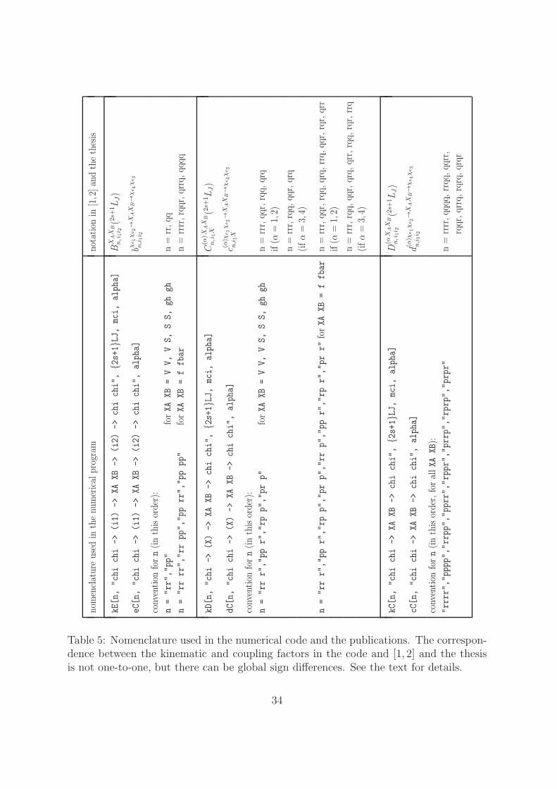
nomenclatureused
inthenu
merical
program
notation
in[1,2]an
dthethesis
kE[n,
"chi
chi
->(i1)
->
XAXB
->
(i2)
->
chi
chi",
2s+1LJ,
mci,
alpha]
BX
AX
B
n,i
1i 2(2
s+1LJ)
eC[n,
"chi
chi
->(i1)
->
XAXB
->
(i2)
->
chi
chi",
alpha]
bχe1χe2→
XAX
B→
χe4χe3
n,i1i 2
convention
forn(inthisorder):
n=
"rr","pp"
forXA
XB=
VV,V
S,
SS,
gh
gh
n=
rr,qq
n=
"rr
rr","rr
pp","pp
rr","pp
pp"
forXA
XB
=f
fbar
n=
rrrr,rqqr,qrrq,qq
kD[n,
"chi
->(X)
->
XA
XB
->
chi
chi",
2s+1LJ,
mci,
alpha]
C(α
)X
AX
B
n,i
1X
(2s+
1LJ)
dC[n,
"chi
chi
->(X)
->
XA
XB
->
chi
chi",
alpha]
c(α)χ
e1χe2→
XAX
B→
χe4χe3
n,i1X
convention
forn(inthisorder):
n=
"rr
r","pp
r","rp
p","pr
p"
forXA
XB
=VV,
VS,
SS,
ghgh
n=
rrr,qq
r,rqq,
qrq
if(α
=1,2)
n=
rrr,rqq,
qqr,qrq
(ifα=
3,4)
n=
"rr
r","pp
r","rp
p","pr
p","rr
p","pp
r","rp
r","pr
r"forXA
XB=
ffbar
n=
rrr,qq
r,rqq,
qrq,
rrq,
qqr,rqr,qrr
if(α
=1,2)
n=
rrr,rqq,
qqr,qrq,
qrr,rqq,
rqr,rrq
(ifα=
3,4)
kC[n,
"chi
chi
->XA
XB
->
chi
chi",
2s+1LJ,
mci,
alpha]
D(α
XAX
B
n,i
1i 2
(2s+
1LJ)
cC[n,
"chi
chi
->XA
XB
->
chi
chi",
alpha]
d(α)χ
e1χe2→
XAX
B→
χe4χe3
n,i1i 2
convention
forn(inthisorder,forallXAXB):
"rrrr","pppp","rrpp","pprr","rppr","prrp","rprp","prpr"
n=
rrrr,qq
qq,rrqq
rr,
rqqr,qrrq,rqrq,qrqr
Table 5: Nomenclature used in the numerical code and the publications. The correspon-dence between the kinematic and coupling factors in the code and [1, 2] and the thesisis not one-to-one, but there can be global sign differences. See the text for details.
34
References
[1] M. Beneke, C. Hellmann, and P. Ruiz-Femenia, JHEP 1303 (2013) 148,arXiv:1210.7928 [hep-ph].
[2] C. Hellmann and P. Ruiz-Femenia, JHEP 1308 (2013) 084, arXiv:1303.0200[hep-ph].
[3] M. Beneke, C. Hellmann, and P. Ruiz-Femenia, arXiv:1411.6924 [hep-ph].
[4] M. Beneke, C. Hellmann, and P. Ruiz-Femenia, arXiv:1411.6930 [hep-ph].
35


![arXiv:1409.3930v3 [hep-ph] 23 Mar 2015 · Particle (LSP) neutralino, we have the bino-wino, LSP neutralino-stau, and LSP neutralino-tau sneutrinos coannihilation scenarios, and the](https://img.dokumen.tips/doc/110x75/60d44719e69ef1617d11d9f8/arxiv14093930v3-hep-ph-23-mar-2015-particle-lsp-neutralino-we-have-the-bino-wino.jpg)
![and Neutralino Masses in the MSSM - arXiv.org e-Print …1107.5218v1 [hep-ph] 26 Jul 2011 On the On-Shell Renormalization of the Chargino and Neutralino Masses in the MSSM ∗Arindam](https://img.dokumen.tips/doc/110x75/5b34a5b17f8b9abc218c631d/and-neutralino-masses-in-the-mssm-arxivorg-e-print-11075218v1-hep-ph-26-jul.jpg)


![Neutralino Relic Density including Coannihilations - arXiv · Neutralino Relic Density including Coannihilations ... the Gondolo and Gelmini [10] formulas to solve the Boltzmann equation](https://img.dokumen.tips/doc/110x75/5c662c4a09d3f2d8348bc9ec/neutralino-relic-density-including-coannihilations-arxiv-neutralino-relic.jpg)