Some of the problems and techniques involved in manpower ... · Methods for Manpower ... Some of the problems and techniques involved in manpower forecasting ... Sometimes "prediction"

DOCUMr NT R r v M

ED 025 661 VT 007 611

By- Morton, J.E.On Manpower rorecasting. Methods for Manpower Analysis, No.aUpjohn (W.E.) Inst. for Employment Research, Kalamazoo, Mich.Pub Date Sep 68Note- 57p.Available from- W.E. Upjohn Illstitute for Employment Research, 1101 Seventeenth Street, N.W. Washington,D.C. 20036

EDRS Price MF-$0.25 HC-$2.95Descriptors- Economic Research, *Employment Projections, *Manpower Needs, Mathematical Models,*Measurement Techniques, Prediction, *Research Criteria, *Research Methodology, Research Problems

Some of the problems and techniques involved in manpower forecasting arediscussed. This non-technical introduction to the field aims at reducing fears of datamanipulation methods and at increasing respect for conceptual, logical, and analyticalissues. The major approaches to manpower forecasting are explicated and evaluatedunder the headings: (1) Some Curve-Fitting, Techniques, involving essentially themethods of population forecasting, (2) Dire"t Manpower Forecasts, which make use ofmanpower variables only, (3) Derived Manpower Forecasts, which rely on safelypredictable variables (population or economic) which arz,-- associated with manpowervariables, and (4) Econometric Models, which mathematically depict relationships ofsingle or multiple variables. An introductory section discusses the role of manpowerforecasting and its historical development. The concluding section reviews theforecasting techniques in terms of the following dichotomies: (1) short-term versuslong-term forecasting, (2) stochastic versus the deterministic approach, (3) pointversus interval forecasts, (4) unconditional versus conditional forecasts, and (5)first-order versus higher-order forecasts. (ET)

Methods for Manp`ower Analysis

`.1

j. E. Morton2 -r

mot-

0-

r

alJr,

r;t1PIO NINSTITUTE*OE zliruCrrivilerREsEA1OR p4q41w44444-NATARIalinsia 19141w t

L

Methods for Manpower Analysis No. 2

0025661

ON MANPOWER FORECASTING,

By

J. E. MORTON

U.S. DEPARTMENT OF HEALTH, EDUCATION & WELFARE

OFFICE OF FDUCATION

THIS DOCUMENT HAS BEEN REPRODUCED EXACTLY AS RECEIVED FROM THE

PERSON OR ORGANIZATION ORIGINATING IT. POINTS OF VIEW OR OPINIONS

STATED DO NOT NECESSARILY REPRESENT OFFICIAL OFFICE OF EDUCATION

POSITION OR POLICY.

September 1968

E.'ilpioinuinstiite.for Employment Research300 Sio*Uth Westnedge AvenueKalamazoo, Michigfer-49007

The Board of Trusteesqf the

W. E. Upjohn Unemployment Trustee C. porark

HARRY F. TURBEVILLE, Chairman

I,AWRENCE N. UPJOHN, M.D., Honorary Chairman(deceased)

F. GIFORD UPJOHN, M.D., Vice ChairmanDONALD S. GILMORE, Vice Chairman

D. GORDON KNAPP, Secretary-TreasurerMRS. GENEVIEVE U. GILMORE

ARNO R. SCHORER

CHAR! ES C. GIBBONS

PRES7ON S. PARISH

MRS. HAROLD J. MALONEY

C. M. BENSON, Assistant Secretary-Treasurer

The Statrof the Institute

HAROLD C. TAYLOR, PH.D.Director

HERBERT E. STRINER, PH.D.

Director qf Program Development

Kalamazoo Office

RONALD J. ALDERTON, B.S.SAMUEL V. BENNETT, M.A.EUGENE C. MCKEAN, B.A.

Washington Office

E. WIGHT BAKKE, PH.D.A. HARVEY BLLITSKY, PH.D.SAUI. J. BLAUSTEIN, B.A.ROSANNE E. BURCH, B.A.SAMUEL M. BURT, M.A.SIDNEY A. FINE, PH.D.

HAROLD C. TAYIAM, PH.D.HENRY C. THOLE, M.A.W. PAUL WRAY

HENRY E. FIOLMQUIST, M.A.J. E. MORTON, JuR.D., D.Sc.MERRILL G. MURRAY, PH.D.HAROLD L. SHEPPARD, PH.D.IRVING II. SIEGEL, PH.D.HERBERT E. STRINER, PH.D.

AMIRIMIOWPM.0.111.11OMMI=M.N.

PrefaceThis paper is intended to serve as a non-technical introduction for thegeneral manpower analyst who, not himself an expert in the use of fore-

casting techniques, is desirous to form an opinion about some of the prob-lems and techniques involved; in particular, it aims at reducing fears ofdata manipulation methods and at increasing respect for conceptual,logical and analytical issues.Since the field of manpower forecasting is in a state of flux, and includes

methods borrowed from early demographic writings as well as from themost recent econometric literature, it should be pointed out that themanuscript was completed early in Spring 1967 and that, accordingly itreflects the state of the arts as of approximately that time.

III

The W. E. Upjohn Institutefor Employment Research

THE INSTITUTE, a privatel) sponsored nonprofit researchorganiiation, was established on Jul) 1, 1945. It is anactivity of the W. E. Upjohn Unemplo)ment TrusteeCorporation, which was fmmed in 1932 to administer afund set aside by the late Dr. W. E. Upjohn for the pur-pose of carrying on "research into the causes and effects

of unemployment and measures for the alleviation of

unemployment."

One copy of this bulletin may be obtained without

charge from the Institute in Kalamazoo or from theWashington office, 1101 Seventeenth Street, N.W.,

Washington, D.C., 20036. Additional copies may beobtained from the Kalamazoo office at a cost of 50 centsper copy.

iv

ContentsPage

I. THE ROLE OF MANPOWER FOlcZCASTING 1

II. SOME CURVE-FITTING TECHNIQUES 5

III. DIRECT MANPOWER FORECASTS 20

IV. DERIVED MANPOWER FORECASTS 25

V. ECONOMETRIC MODELS 32

VI. RETROSPECT AND PROSPECT 46

On Manpower Forecasting

I. The Role of Manpower ForecastingThe forecasting of manpower and of manpow er components has a longand distinguished history. From the time of the early demographers,numerical outlook estimates of the population and related variables haveinfluenced the opinions of social philosophers, statisticians, politicians,and administrators, as well as the public at large. In the past few years, aperiod during which the term "manpower" has acquired technical status,forecasts of labor force and employment have become increasingly fa-miliar.' ihey are nowadays used often as a basis for forecasting othermajor economic measures, e.g., the Gross National Product (GNP).

The President's Committee on Manpower, established to assist incarrying out federal responsibilities under the Manpower Developmentand Training Act of 1962, has shown a strong interest in the design andconstruction of consistent govermental forecasts of the nation's labor re-sources and needs. This interest is reflected in a 1967 repert of a WorkingGroup established by the Bureau of the Budget.' The group's activities,in turn, have stimulated the preparation of a comprehensive and thought-provoking commentary on long-range forecasting of the labor force."'

The objective of forecasting is to reduce our uncertainty about futureevents.4

Forecasting, thus, is the art of forming expectations and antici-See, e.g., H. Goldstein, "Projections of the Labor Force of the United States, "in

U. S. Congress, Senate Committee on Labor and Public -7elfare, Hearings, Nation'sManpower Revolution, pt. 5 (1963) and "Projections of Manpower Requirements andSupply," Industrial Relations, Vol. 5 (1966); S. L. Wolfbein, "Manpower in the UnitedStates with Projections to 1970," in U. S. Congress, House Committee on the Judiciary,Special Series No. 3 (1962); B. Grais, Forecasting of the Active Population by Occupationand Level of Skill (Paris: Organization for Economic Cooperation and Development, P66);U. S. Bureau of Labor Statistics, Projection 1970, Bulletin No. 1536, 1966; U. S. Depart-ment of Labor, Manpower Projections, a bibliography, 1966.

U. S. Department of Labor, Manpower Administration, Manpower Projections: AnAppraisal and a Plan for Action, August 1966. In this publication there also can be foundexamples of the application of manpower forecasting to a wide spectrum of matters rele-vant to national policy. For bibliographical references, see pp. 34 ff.

3 U. S. Bureau of Labor Statistics, Lona-Range Projection of Labor Force, by Dennis F.Johnston, September 1967; mimeographea,

Two terms are available: "forecasting" and "prediction." Both terms are in generaluse. Sometimes "prediction" is used for the more formal and "forecasting" for the moreinformal proceduressee, e.g., Jay W. Forrester, Industrial Dynamics (Cambridge, Mass.;Technology Press, MIT, 1961); sometimes "prediction" is used for vague conjecture and"forecasting" for quantitative procedures based on specific observation and information--see Robert G. Brown, Stnoothing Forecasting and Prediction of Discrete Time Series(Englewood Cliffs, N. J.: Prentice-Hall Inc., 1963). The term "forecasting" seems tohave been more widely used in book titlesC. W. F. Butler and Robert A. Kavesh, HowBusiness Economists Fnrecast (New York: Prentice-Hall, Inc., 1966); E. Bratt, BusinessCycles and Forecasting (5th ed.; Homewood, Ill.: Richard D. Irwin, Inc., 1961); and Milton

1

VP

pations in which we have greater confidence than in the unguided andunsupported guess. Whether because of the urge of idle curiosity, or thenecessity to arrive at an important decision, man has since ancient timessought to unveil the future; in this attempt to discount the tomorrow, andto strengthen confidence in his own expectations, he has been looking tooracles and prophecy, to astrologers and numerologists, and later to morenearly objective and scientific devices for clues and revelation.

In the behavioral sciences the importance of the problem of forecast-ing in the modern sensc was early recognized by demographers and ac-tuaries, who were in many respects predecessors of the students of man-power problems. The construction of life tables, one of the first majorforecasting devices, can be traced to Graunt and Halley, both of theseventeenth century.' Later, in 1783, Richard Price translated the find-ings into actuarial practice. During the nineteenth century the first docu-mented attempts were undertaken to make projections of populationtotals as well as of vital rates on the basis of mathematical functions.'

In the area of ec-nomics during the second half of the last centuryand the first quarter or so of the twent: +b, interest in prediction andforecasting techniques originated with business cycle and time seriesanalyses.

The study of repetitive "commercial crises" resulted in the identifica-tion of apparent oscillatory movements or "cycles." Anticipating turningpoints of the wavelike movement assumed considerable practical impor-tance, and the business cycle became a basic concept for analysis andinterpretation of these recurrent economic movements.'

By the first quarter of this century the problem of the economic cycles

H. Spencer, Collin J. Clark, and Peter W. Hoguet, Business and Economic Forecasting(Homewood, Ill.: Richard D. Irwin, Inc., 1961). H. Theil's recent book, Applied EconomicForecasting (Amsterdam: North-Holland Publishing Company, 1966), refers in the indexunder "forecasting" to "prediction." C. F. Christ's recently published Economic Modelsand Method (New York: John Wiley & Sons, Inc., 1966) uses the two terms interchange-ably.

5 John Graunt, Natural and Political Observations Made Upon The Mortality (London:1662; reprinted in Baltimore: The Johns Hopkins Press, 1939); and E. Halley, An Estimateof the Degrees of Mortality .... , Philosophical Transactions of The Royal Society ofLondon (London: 1693; reprinted in Baltimore: The Johns Hopkins Press, 1942).

b See especially P. F. Verhulst, "Notice sur la loi que la population suit dans son ac-croissement," in Correspondance mathimatique et physique publiee par A. Quetelet,Tome X (Bruxelles: M. Hayez, 1838) and "Recherches mathématiques sur la loi d'ac-croissement de la population," Nouveaux memoirs de l'Acadimie Rot.ale des sciences etbelles lettres de Bruxelles, XVIII, 1 (1845); and H. Gylden FórsqkringsforeningensTidskrift (Stockholm, 1878); see also H. Cramer and H. Wold, "Mortality Variations inSweden," Skandinavisk A ktuarietidskrift, Uppsala 161 (1935).

7 See, e. g., Clement Juglar, Des crises commerciales et leur retour periodique (Paris:1862; reprinted in New York: Augustus M. Kelley, 1967).

2

woo

had become one of the central topics of economic theory and analysis!'Once the cyclical nature of economic change was believed to have beenestab1i4ted, growing interest manifested itself in the practical questionof how to forecast the behavior of this dynamic system. The caref'l de-scription and decomposition of economic time series into various compo-nentsthe long waves,' the shorter cycle, and the still shorter seasonalcomponentoccupied leading economists of the time.w

In this country the new insight generated, at an early stage, devicesand schemes for use in practical business forecasting which later (1917)led to the famous barometer system of the Harvard Economic Service."From the United States these forecasting services and institutions spreadover most of Europe, the best known being the London and CambridgeEconomic Service, established in 1923, and the Institut fuer Konjunk-turforschung in Berlin established two years later.

This early enthusiasm was damped by those who raised the funda-mental question of forecastability on the continent, among others byKondratieff and Morgenstern--and shortly thereafter by the unfore-seen disaster of 1929.2 But by the mid-thirties the scene was set for thereappearance of forecasting and the study of economic time series as alegitimate subject deserving most serious attention in economic andstatistical theory and analysis.

Special concern about the particular problem of manpower predictionis relatively recent. But its late appearance has made manpower fore-casting the beneficiary and captive of earlier experiences and effortselsewhere, notably in demography and in the empirical analysis of busi-ness cycles. This venture into the domain of prognos. cationat first veryslowly and only gradually expandingreceived a potent fillip during thedepression of the thirties. The unemployment problem, and the resultingattempts by government to cope with it, required decisions, manpowerpolicies, and strategies predicated on "early warning systems" and onmore or less clearly visualized effects on the future supply-demand

8 See, for instance, Henry L. Moore, Economic Cycles (New York: The MacMillanCompany, 1914) and Forecasting Yield and Price of Cotton (New York: The MacmillanCompany, 1917).

9 N. D. KondratiefT, "Die Langen Wellen der Konjunktur," Archiv fur Sozialwissen .schaft und Sozialpolitik, LV I (1926).

1" Wesley Mitchell, Business Cycle (New York: National Bureau of Economi: Research,1927); and much of the literature produced by the staff of the National Bureau of EconomicResearch.

" For earlier attempts in this direction see, e.g., R. W. Babson Reports since 1904 aildThomas Gibson's Stock Market Forecasts since 1907 The Harvard barometer system isbest described in the works of Warren M. Persorw,.

12 N. D. KondratiefT, "Das Probizin der Prognose" Annalen der Betriebswirtschaft,Vol. I (1927); and Oskar Morgenstern, Wirtschaftsprognose, eine Untersuchung ihrerVoraussetzungen und Nuetzlichkeit (Vienna: J. Springer, 1928).

3

situation. A similar contingency, produced by a reversal in the laborsupply-demand discrepancy during the war and postwar years of theforties, further accentuated the need for better and more detailedmanpower forecasts.

rimong the present problems, to the solution of which manpowerforecasts are supposed tv contribute, are: the future demand for workers;the expected composition of the labor force with reference to educationaland training need; the feasibility of new programs and ventures in termsof availability of required skills; early warning systems foreshadowing dis-ruptive effects of automation; and the development of vocational guidanceand occupational outlook information. Labor force forecasts also play animportant role in developing general economic projections.

Then there are the manpower forecasts which are not directed to aspecific decision problem and which, by analogy with government statis-tics, might be termed general-purpose forecasts. There are also the fore-casting objectives that are best attributed to the "fears and fascinationof the future,' and the broad interests illustrated by the French groupof "futuribles" and their principal exponent, Bertrand de Jouvelel."

These are macroeconomic objectives, but manpower forecasting hasalso found its way into microeconomic practice. Many smaller but spe-cialized firms, large corporations, and of course, individuals are aware ofthe uncertainties of future labor markets. Consequently, it has becomeimportant for the forecaster to form an opinion about how best to copewith the future in terms of optimum utilization of employees, and otherpersonnel policy matters aimed at the long run. Because of uncertaintiesinherent in forming an opinion, decisions about such matters are some-times predicated on the earlier mentioned type of macro forecasts; butoften special micro predictions must also be prepared, tailormade forthe particular purposes at hand. Among them should be mentionedforecasts of the need by a given company for highly trained, specializedper onnel; anticipation of labor turnover rates; and process analysis ap-plie absenteeism, accidents, and sickness."

in view of this vast array of diverging objectives and uses of manpowerforecasts, it is not surprising to find widely differing methods and schemesof forecasting, ranging from quite primitive to highly sophisticated ones.

H Daniel Bell, "The Study of the Future," in The Public Interest (1965), as quoted byGarth L. Mangum and Arnold L. Nemore, "The Nature and Functions of ManpowerProjections," Industrial Relations, v. 5, n. 3 (May 1966).

14 See, for instance, the stimulating tract by Bertrand de Jouvenal, The Art of Con-jecture (New York: Basic Books, Inc., Publishers, 1967).

See, e.g., Ore Lunberg, Random Processes and Their Application to Sickness andAccident Statistics (Uppsala: Almquist Wiksells, 1940), and the copious recent literaturein operations research and the management sciences. Methods other than those used inmacro prediction will not be discussed in this paper but be deferred to a later occasion.

4

But none of them is fully satisfactory, and much criticism and doubthave been expressed with respect to methods as well as concepts!'Nevertheless, forecasting, in one form or another, has become a basicand neLt.ssai y constituent of decision making in modern society. It is anessential ingredient in the choice of man's responses to a dynamic en-vironment. All forecasting efforts, by whichevei method, have one ele-ment in common: the search for relative stabilities and invariances ofrelationship. These suspected relationships may be simple ones betweenthe phenomenon to be forecast and the data (not necessarily quanti-tative) to be used as "predictors." With increasing acceptance of factual-ism and quantification, it was perhaps to be expected that sooner or laterthe quest would be directed toward discovering such stable dependenciesof "predictand" on "predictors" in terms of original values of variables,rates of change, transformations of variables, and even entire systems ofequaLions.

However complex the resulting methods and models, their forecastingpowers stand and fall with the validity of the assumed or implied in-variances. No procedure for a priori validation of such presuppositionshas yet been found. Although comparison of realization with forecastcan help refute the soundness of the method that produced the particu-lar forecast, the reverse generally cannot be inferred with certainty.Even the more recent application of the "science of uncertain inference"to the study of economic time series has not, by and large, yielded satis-factory results with respect to forecasting of economic time saies. Butthere are better and worse forecasting methods, and there are more andless useful techniques. All in all, however, socioeconomic forecastingstill remains an art.

If. Si-me Curve-Fitting Techniques

As suggested above, manpower forecasting has developed in close his-torical and logical affinity with population forecasting. The manpowerforecaster therefore needs to be aware of population forecasting methodsand techniques.

Among the simplest expressions used in demographic forecasting arethe polynomials,' beginning with the polynomial of degree one, i.e., the

16 For a recent and succinct discussion of some of the issues, see Lee Hansen and Her-bert E. Striner, "The U. S Manpower Future," Proceedings of the Eighteenth AnnualWinter Meeting of the Industrial Relations Research Association (Madison: The As-sociation, 1966)

A polynomial can be expressed by the equation P = a + bT = cf dT' + ,

where P might stand for population, T for time (say, calendar years, and a, b, c, d, ,

are coefficients. The highest power of T whose coefficient is not zero determines the degreeof the polynomial; thus P = a + bT is a polynomial of degree one, or the equation of a

5

straight line. An early example in this country is Abraham Lincoln'sprojection by straight-line extrapolation of the population growth between1790 and 1860 to 1925;" even after a downward revkion, he thus obtained'1.n estimate of 250 million. It is of course easy to criticize ex post factosuch simple procedures; nevertheless, there are many instances in whichlinear projections are of interest to the manpower analyst because ofsimplicity, plausib lity for short-term forecasting, or lack of a betterhypothesis. For in;tance, a linear estimating equation may suffice whenchanging labor force participation rates are to be projected over theshort run. The linear extrapolation rnay be comidered an approximationto the unknown nonlinearity an approximation that is better the shorterthe forecasting horizon.

Several techniques for fitting a straight line to empirical data areavailable, among them tht . method of selected points and the method ofleast squares.

linear trend characterizes a relationship between the particularob.:erved variable, say, population (P) and time (T) so that both P andT progress by constant absolute differences. In other words, both P andT form an arithmetic progression. Since time is conventionally measuredin equal intervals, e.g., years, quarter), or months. our attention is cen-tered only on P. Setting up a difference table, we observe the first dif-ferences in the successive P observations. If they are constant, or nearlyso, the second differences tend to vanish. Using a hypothetical example(see table 1), we find the second differences (.1-) to be "small" indeed.We may therefore wish to fit a straight line.'

In the method of selected points, it is useful to plot the data (seeDiagram 1). The selection of points is greatly facilitated by first fitting aline by inspection. The closer the points actually do cluster about sucha line, the easier it will obviously be to agree on such a line. Once thepoints are plotted, we select any two (preferably two distant ones) andread off their coordinates. In the example, points P:2 and PAI`8, for theyears 1952 and 1958, respectively, were selected. (The asterisks indicate"estimated" quantities, i.e., those on the trend line, not the actually

observed population figures.) The yearly increment is or1958 1952

55 44 11=6

. Thus, the constant annual difference (the slope of the line6

in the diagram) is 11 = 1.83.6

straight line, where a indicates the value of P at T 0, and b is the "slope," i.e., the incre-ment, which is constant, or decrement in P per unit increase in T.

J. J. Spengler, "Population Prediction in Nineteenth Century America," AmericanSociological Review, I (1936).

3 See also F S. Acton, Analysis of Straight-Line Data (New York: John Wiley & Sons,Inc., 1959).

6

Table 1

A Htpothetical 1950 1960 Population(in millions)

Year P tP 11 t2P

1950 38 5 5 15 190 625 9501951 43 1 4 4 16 172 256 6881952 441 / 1 3 9 132 81 3961953 46 0 / 2 4 92 lo 1841954 46 2 / 1 1 46 1 461955 48 2 0 0 0 0 0 01956 50 1 0 +1 1 50 1 501957 52 1 0 +2 4 104 16 2081958 55 3 1 +3 9 165 81 4951959 58 3 0 +4 16 132 256 9281960 5(1

11 +5 25 195 625 1,475

539

/...110 214

1117-10(

1,958 5 420

If ene prefers a more foi mal criterion of best lit, he may choose theso-cafied least-squares principle.' Accordingly, a best fitting line is theone about which the squared dcsiations of the observations are smallerthan about any other such line. To simplify the mechanics, the "origin"of the (Nervations will be shifted to thu arithmetic mean of T. Putdifferently, instead of measuring time in actual units, say, calendar .ears,we measure it in terms of deviation from the middle of the period, T, so

it t T T. Under these conditions it turns out that the slope orannual increment, equals .

ItP 214Taking the same example, we find that , =110

= 1:95.It'This value differs, but not very much, from the slope or annual incre-

ment found earlier, 1.83.To write the equation of the linear trend using the slope-intercept form,

P = a + bt, we need to know, in addition to the slope of the line (b),the coordinates of one point on the line. Such a point is a in the aboveequation. In particular, a.is the value of P* at the "origin" of the series.If the origin is taken at r (for which t = 0), the least-squares principle

Irving H. Siegel, "Productivity Measures and Forecasts for Employment andStabilization Policy," in Sar A. Levitan and Irving H. Siegel, eds., Dimensions of ManpowerPolicy: Programs & Research (Baltimore: The Johns Hopkins Press, 1966), pp. 269-88.

1952 1953 1954 1955 1956 1957

Diagram 1Hypothetical 1950 OW hip:datum

(in millials)

1958 1959 1960

yields a -- IP. That is, the least-squares line passes through the arithmetict/

mean of the observations.IP 539

Since in our example11

----- 49, the equation of the least-squares

line is P* 49 + 1.951 (with origin at t = 0, i.e., at 1955).Had we used the selected-points method, for which we had found the

slope h ---- 1.83, the value of a would have to be read off Diagram 1.Using again T as the origin, we find that a = 49.5, and that the equationof the trend is P* = 49.5 + 1.831, which is similar to, but not identicalwith, the one found by the method of least squares.

As already mentioned the implication of the linear trend is that thevariable P is a linear function of time. In other words, its averageincrease or decrease per unit of time is assumed constant over time.

It was soon observed that, in considering longer stretches, the popula-tion increment per unit of time did not remain constant, especially fora dynamic nation such as the United States. In the quest for a flexible

but simple descriptive device, polynomials of higher than first degreesoon attracted the attention of for.casters.

Early interest in fitting polynomials of higher degree to populationchanges was aroused by the mathematician and astronomer Pritchett,who fitted a third-degree polynomial to the population of the United

8

States. On the basis of this equation he made forecasts for 10 centurieshence, arriving at 222 million for 1960, and at 41 billion for 2900."

Although nowadays one would hardly use polynomials for projectingpopulation totals over long periods, the method is of interest for fittingcurves over shorter periods to selected manpower variables. Polynomialsof varying degree provide a very flexible means for fitting nonlinearfunctions to observational data.

Thf; (n lth) difTerences of an n degree polynomial vanish a usefulproperty for experimenting with functions to fit time-series. Polynomialsthus can be regarded as a flexible, curved ruler; a polynomial of degreen has n 1 points of inflection. In fitting a polynomial of degree two tothe data in our example by the method of least-squares, we obtain atrend equation of the,form:

1; PP = a + bt + et- , in which a Ct

fat' P=

tPI , 2nsl )

Substituting in these expressions, we find:

a = 53913

85 48.65

114b = 1.95, and11059,620 59,290 59,290 330

c 21,538 12,100 9438

Hence, the sought trend equation is: P* = 48.65 ± 1.95t .035r.The greater flexibility of polynomials is not necessarily an advantage

from th t'. manpower analyst's point of view. The closer fit of functions tomore or less erratic oscillations of economic time series obscures thestructural meaning which is necessary for forecasting. In other words, afunction that closely fits irregular fluctuations of empirical manpowerdata for the past should hardly be assumed to follow the same complexpath in the future unless good theoretical reasons suggest such a course.In socioeconomic situations, we rarely ever are justified, a priori, toexpect such behavior! Where time series are to be decomposed intocomponents that separate systematic from more nearly accidental

H. S. Pritchett, "A Formula for Predicting the Population of the United States,"Transactions of the Academy of Sciences of St. Louis (1890).

Hence the problem of overfitting, as it is called by H. 0. A. Wold in his Study Weekon The Econometric Approach to Development Planning (Amsterdam: North-HollandPublishing Company, 1965), Chapter 2; he properly relegates this pitfall to the "nonsensedepartment of statistical method."

9

movements, other smoothing devices are available. Should the readerwish to apply higher-degree polynomials to fit observational data forminga time series, he may use the method of orthogonal polynomials. Theprinciple of fit involved is again the least-squares criterion, but thetechnique is considerably simpler than that for the classical least-squaressolution if a set of appropriate tables is available. Among the advantagesof the method is that the necessary coefficients for higher polynomialsmay be completed in successive steps; thus a polynomial of degree n canbe changed to one of the n ± It" degree by computation of just one Adi-tional coefficient. This is a significant advantage in experimentationwith polynomials of uncertain degree.

Exponential functions are most widely used in fitting curves to agrowth phenomenon in the social sciences. Various polynomials arecharacteriled by the constancy of their first or higher order differencesin the dependent variable. If the independent variable (time) proceedsby equal steps, exponential functions desebe a similar constancy inthe pattern of change in relative rather than absolute terms. The ex-ponential is therefore a useful device for describing a time series for whichthe additions are in turn a function of the magnitude of the variable; inother words, large values of the variable are associated with largeincrements, and conversely. Accordingly a series that increases at a con-stant percent rate can be conveniently presented by the simpk exponentialfunction or its graph.

The most common example for exponential patterns of growth is theso-called organic law: (also called compound interest law). Unlike thelinear function for which both variables proceed as an arithmetic series,one variable (say, time) in the exponential case progresses arithmetically;the other (say, P) geometrically. Such a relationship between two vari-ables, e.g., P and T ean be expressed by P = ab' . Taking logarithms, weobtain log P = log a T log b, which gives log P as a linear function oftime. In other words, if we plot logs of P instead of the original valuesagainst time, we shall obtain the graph of a straight line. To simplify theplotting we may, rather than look up the logs of P, use graph paperruled along the vertical axis in logarithms-----the well known semilogarith-mic paper. This simple transformation not only facilitates the diagnosis of

Tables with instructions for use in fitting by the method of Orthogonal Polynomialscan be found in R. A. Fisher and Frank Yates5tatistical Tables fbr Biological, ,..1gricul-tural, and Medical Research (2nd ed.; London: Oliver & Boyd, 1943); W. Beyer, ed.,Handbook t),f Tables Ihr Probability and Statistics (Cleveland: The Chemical PublishingCompany, 1966); and R. L. Anderson and E. E. Houseman, Tables Qf Orthogonal Poly-

nomial Values Extended to N = 104, Research Bulletin 297 (Ames, Iowa: AgriculturalExperiment Statior, Iowa State College of Agriculture and Mechanic Arts, 1942). For anot-too-technical description of the method, see also W. E. Milne, Numerical cakulus(Princeton: Princeton University Press, 1949), Chapter IX.

So-called because many populations in biology follow this pattern of growth, e.g., cul-tures of bacteria, populations of animals, and the like.

10

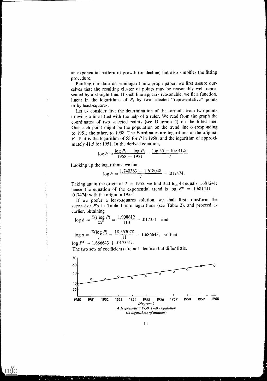
an exponential pattern of growth (or decline) but also simplfies the fittingprocedure.

Plotting our data on semilogarithmic graph paper, we first assure our-selves that the resulting 'luster of points ma., be reasonably well repre-sented by a straight line. If siich line appears reasonable, we fit a function,linear in the logarithms of P, by two selected -representative" pointsor by least-squares.

Let us consider first the determination of the formula from two pointsdrawing a line fitted with the help of a ruler. We read from the graph thecoordinates of two selected points (see Diagram 2) on the fitted line.One such point might be the popu!ation on the trend line correspondingto 1951; the other, to 1958. The P-ordinates are logarithms of the originalP that is the logarithm of 55 for P in 1958, and the logarithm of approxi-mately 41.5 for 1951. In the derived equation,

l hlog P.: log P1 log 55 log 41.5

og1958 1951 7

Looking up the logarithms, we find1.740363 1.618048

log b .017474.7

Taking again the origin at T = 1955, we find that log 48 equals 1.681241;hence the equation of the exponential trend is log P* = 1.681241 +.0174741 with the origin in 1955.

If we prefer a least-squares solution, we shall first transform thesuccessive P's in Table 1 into logarithms (see Table 2), and proceed asearlier, obtaining

1(i 102 P) 1.908612log b = .017351 and

110

I(log P) 18.553078log a

n 111.686643, so that

log P* = 1.686643 + .017351t.The two sets of coefficients are not identical but differ little.

1950

1 I I I I I I I I

1951 1952 1953 1954 1955 1956 1957 1958 1959Diagram 2

A Hypothetical 1950 1960 Population(in logaritluns of millions)

11

1960

Table 2

A Hypothetical 1950 1960 Poptdatiem(in logarithms of millions)

Year t Log P t log P

1950 5 1.579784 7.898920

19.f 1 4 1.633468 6.533872

1952 3 1.643453 4.9303591953 1 1.662758 3.2355161954 1 1.662758 1.662758

1955 0 1.681241 0.000000

1956 1 1.698970 1.698970

1957 2 1.716003 3.432006

1958 3 1.740363 5.221089

1959 4 1.763428 7.053712

1960 5 1.770852 8.854260

18.553078 1.908612

Translating these logarithmic equations of the exponential into theirconventional, nonlogarithmic form, P = , we obtain (after looking up

the appropriate antilogs) = 48 (1.04) and 48.6 (1.04)`, respectively,where a is the value of P* for t = 0, i.e., 1955. Here b = 1.04 is the growthtatio, or r, in the geometric 3eric3 P, Pr, Pr' Pr' Letting r I -I-

where i is the rate of increase of the population expressed as a decimalincrement, we recognize the compound interest formula of the accountantand may write the above exponential as Pn = Po (1 + !n our ex-ample, subscript n refers to the year to be estimated, subscript 0 to thebase year, and i to the percent rate of growth,j i.e., approximately 4percent per annum.

The technique of fitting curves to manpower observations is evidently

9 If interest is compounded k times year, so that

P0(1 + )kl ,

it could be shown that as k increases beyond all bounds, (i.e., as compounding takes place

1

more and more often) the expression (1 +k ) reaches a limit called e (approximately

2.7183). Flence we may also write P = P0e", a formula representing the so-called compound

interest law or the law of organic giowth and reflecting continuous exponential change.

12

a simple enough matter.'" A quite different matter, however, is the choiceof an appropriate function or line.

To illustrate this point, we project the several lines obtained above,all of which appear to fit the observed data quite well, to the year 1975.Substituting 20 for t, in the several equations (since the origin was takenat 1955, 1 20 for 1975), we obtain:

linear-trend values of 86.1 and 87.8 million for the visuakselected-points method and the least-squares method, respectively;exponential-trend values of 107.4 and 108 million for the two meth-ods, respectively; and a second-degree polynomial value of 101.7million.

Thus, although different fitting techniques may give sufficiently similarestimates, the discrepancies resulting from the choice of different func-tions are commonly quite pronounced. Unfortunately, no simple auto-matic procedure exists for answering the question as to the "proper"function to use. A thorough understanding of the nature of the under-lying process a knowledge of the fundamental relationships to be de-scribed is nee&d. The manpower analyst needs a valid theory ratherthan mere access to empirical data; and it is at this point that he mayenvy the occasional scientist whose theory enables explanation of thevery mechanism or process he *ishcs to predict. This, of course, doesnot diminish the importance of manpower forecasting, which is more ofan art rather than a science.

For the purposes at hand, the lack of a ceiling diminishes the plausi-bility of simple exponential patterns of growth. The exponential functionhere ciisidered increases without limit. It would be easy enough, how-ever, to provide for such a ceiling in the formula for exponential growth.One particularly simple possibility is to introduce a constant, say, L, toserve as an upper limit toward which the function tends without everquite reaching it. Consequently, one might use the function Y = L ab' ,

where L is the just-mentioned upper "asymptote"; a is negative (if itwere positive, the curve would approach L as a lower limit), and b ispositive, but less than 1. The curve is concave downward and graduallytapers off in the right-hand upper corner as it approaches 1, the upperlimit."

For manpower projections this modification of the exponential hasnot found favor. It might be of interest, however, in developing economies

I" In practice the technique is even simpler to apply than the above example suggestsbecause any desk calculator with reasonable capacity will permit skipping the intermediatesteps (shown here for expository purposes) and obtaining the needed totals immediately.

" A treatment in nontechnical language can be found in F. E. Croxton and D. J.Cowden, Applied General Statistics (New York: Prentice-Hall, Inc., 1939 and later).

13

when a target for employment is to be reached gradually after an initialspurt.

Another pattern of growth, an S-curve, also approaches an upperlimit and can be represented by a modification of the simple exponential.This curve is of more direct concern to population and manpower ana-lysts. The growth of certain phenomena advances slowiy at first, thenrapidly, and thereafter tapers off toward an upper asymptote. This typeof change caught the fancy of nineteenth century social scientists, es-pecially during the earlier part, when scientific patterns of thought be-came prominent. Quetelet, the outstanding Belgian social statisticianand astronomer was deeply impressed by the suggestion of stability andinvariance in the social sphere, long thought of as an area not amenableto scientific approaches. Under his influence the Belgian mathematician,P. F. Verhulst, addressed himself to the problem of population growth.In his quest for an explanatory function to help trace population growth,he soon realized the limitation of simple exponential functions and beganto modify them. His ideas attracted attention in the United States abouttwo and a half generations later, when Reed and Pearl independentlydeveloped their law of population:-

From the point of view of prediction, curve-fitting techniques do nctassure discovery of rational trends. The latter are intended as statementsof explanatory, analytical structures rather than mere historical descrip-tion."

In his quest for a mathematical function giving a logical explanationof population growth, Verhulst was deeply influenced by the then-cur-rent Malthusian ideas." He was impressed that populations have atendency to grow gezmetrically at first and that at some point serkAts

obstacles begin to manifest themselves, so that growth is slowed as theprocess cont:nues. The devised function therefore should express a "lawof growth," as in the biological sciences growth acceleration duringthe first half of the process and deceleration but continuing growth during

J. Reed and Raymond Pearl, "On the Summation of the Logistic Curve," Journalof the Royal Statistical Society, Vol. 90 (1927); and R4mond Pearl, Studies in HumanBiology (Baltimore: The Williams & Wilkins Co., 1925). See also G. Udny Yule, "TheGrowth of Population and the Factors Which Control it," Journal of :he Royal StatisticalSociety, Vol. 88 (1925). A few years earlier, unknown to Reed and Pearl, Verhulst had been

rediscovered by L. G. duPasquiersee his article, "Esquisse d'une Nouvelle Th6orie de la

Population," Vierteljahrsschrift der NaturjOrschungs Gesellschaft, 63 (Zurich: 1918).

" The earlier much stressed methodological discrepancy between idiography (descrip-

tion) and nomothesis or nomology (the postulation of laws and stable relationships),though of considerable practical importance in the days of Wilhelm Windelband--- -see his

Die Lehre corn Zufall (1870)---i probably less acute today. In prediction problems, how-ever, the predominance of idiogrt4phy and pragmatic optimism has probably contributedmuch to some of the slipshod approaches that can still be found.

" It was Verhulst who gave the particular function the name, "logistic," which since has

been generally accepted.

14

the second half with population asymptotically approaching some upperlimit.

The logistic curve describes expected change during a completegrowth cycle. The growth rate begins near 0, rises to a maximum, anddeclines again toward 0.

This pattern was found to fh some animal and human populationsextremely well. Pearl successfully applied the function to the growthof experimental populations of drosophila, of saccharomyces, and ofyeast cells; to the individual growth (in terms of body weight) of the malewhite rat; and to the growth of populations in a great many westerncountries, including the United States (1790 1920) and Sweden (17501920).15

The logistic "model," the first deserving the name in the field of popu-lation and human resources, encompasses two, possibly quite different,growth-process types. As Davis observed,111 it seems to express betterand more cogently the growth pattern of populations and colonies ofindependent elements rather than the growth patterns of the organismsthemselves- -e.g., of dynamic structures subject to a "central mechanism,"such as body weight. Are patterns of manpower change in a particularsocioeconomic setting like the biological growth of a group of indivithials,or are they like the growth of an organism, of an ordered structure orsystem subject to autonomous and interdependent responses? As socialstructure develops and loses some of its random aspects, long-rangeforecasting via the logistic would seem a hazardous procedure. Forshorter periods, however, the logistic form of growth may at least be aworthwhile device to ascertain the discrepancy between the actual (per-haps "directed") and the theoretical (free) growth of a population oforganisms.

In essence, the logistic formula is a reciprocal of the earlier mentioned

modification of the exponential, i.e., P = ---1 -T In particular,L ab

P =I

Ler where j(T) = a + bT is a first degree polynomial in 7', and L

again is the kiper limit. A higher degree polynomial can, of course, beconsidered for a better fit,1' but the underlying rationale rapidly be-comes involved and obscure. The first differences of logistic functionvary; and when plotted, form a symmetrical, bell-shaped (not necessarily

Pearl, op. cit. For other biological examples sec, e.g., T. Carson, "Ober Geschwindig-keit und Grasse der Hefevermehrung in Wilrze," Biochemische Zeitschrift, Vol. 57 (1913);or T. B. Robertson, The Chemical Basis of Growth and Senescence (Philadelphia: J. B.Lippincott Co., 1923).

lb Harold T. Davis, The Analysis of Economic Time Series (Bloomington, Indiana:Principia Press, 1941).

" Second- and third-degree polynomials were used to advantage in smoothing observa-tions, reflecting the presence of some "central mechanism" as alluded to earlier.

15

normal) curve with the mode at the point of inflection of the fittedcurve.

To fit tne logistic L

1

to series of reasonable length is not tooe

bothersome with usual desk calculators. As in the earlier illustrations,we may, for example, select equally spaced points and let the functionpass through these points. Three points are needed, since there are threeconstants, L, a and b.

Let us assume that annual observations (Ps) are available for the years1953 to 1967. For convenienee we code the years into T units so thatonly the la .4. digit of the calendar year is used during the fifties and thelast digit plus 10 for the years during the sixties. We select three equi-distant points of time, say T1 = 5 (that is, 1955), at 7 2 = 10 (that is, 1960),and T:3 = 15 (that is, 1965). Next we plot the observations (that is, Ps)and fit a freehand S-shaped curve or any part of such a curve. Fromthe curve thus fitted by inspection to the observational data, we readthe values of the "synthetic" P's corresponding to the years T1, 72, andT. We label the synthetic points H.

To obtain the coefficients in a+hy we use1 + e

2110111112 I112(110 + 112)L = non, 11,-2

L Iloa = log, ---- andII0

1 log, --N 111(L Ho)

These expressions may be written in terms of the base P, rather than c.That is, eahr = logio e(a 1)7); and, since topic, = 0.4343, we haveeaf = 0.4343 (a + b7).

Although only an approximation, the method commonly gives ac-ceptable results. The different constants do vary however with the choiceof the three points.

Other methods are available, among which are Hotelling's least-squares method" and its adaptation by Davis (see footnote 16). Non-

Harold Hotelling, "Differential Equations Subject to Error, and Population Estimates,"journal of the Amerkar Statistical Association, 22 (1927); see also G. Tintner, Econmnetrics(New York: John Wiley & Som., Inc., 1952).

16

technical descriptions can .also be found." Extensive use of the logisticcurve was made by Kuznete to describe economic growth phenomena.

Before !caving the topic of modified exponentials, we call attention toone more modification which resembles the logistic. It too depicts anS-shaped pattern of growth; however, unlike the logistic, the first differ-ences are not symmetrically distributed about a point of inflection.Named after an actuary of the early nineteenth century, the Gompertzcurve was invented primarily with a view to describing certain mortalityphenomena. Gompertz justified the function by reference to the in-ability of organisms, increasing with age, to avoid destructionthis in-ability accounts for the asymmetry of the dimribution of first differ-ences.

21

The equation of the Gompertz function is P = aba; in log form, thisbecomes log P = Log a + c' (log 6), where a is the upper limit and b thedifference between P and the ceiling at the successive points in time,a P. P thus increases with T, but in decreasing relative amounts. Tofit a Gompertz function, we may again select three equidistant timepoints and proceed similarly as in the prescription for fitting a logistic.

Discussion of modified exponentials with reference to the underlyingmechanisms of growth helped to instill a more cautious attitude towardsextrapolation of' past observations. The ensuing quest for rational ratherthan past empirical relatienships marked an important step beyond thepurely empirical descriptive curve-fitting stage. The next forward stridewas taken with the emerging realization that broad aggregates are per-haps too heterogeneous to yield clearly visible and rationalizable pat-terns of change. The quest for improvement then turned toward the de-composition of complex phenomena into simpler ones. The search forcomponc.:i.s proceeded along two lines: components of the populationand their effect on the changing population structure; and componentsof the growth process, of the time series themselves. Both approachesattempt to understand in the small what is not disclosed when phenom-ena are viewed in the large. But micro-information requirements areusually more severe and more difficult to satisfy than macro needs, sothe shift toward disaggregation and decomposition has also shifted theemphasis in needs for statistical data and other information.

More general compulsory vital registration increased the ensuing" Croxton and Cowden, op. cit.; F. C. Mills, Introduction to Statistics (New York:

Holt, Rinehart, & Winston, Inc., 1956), Appendix., and J. D. Smith and A. J. Duncan,Elementary Statistics and Applications. Part I (New York: McGraw-11111 Book Company,1944).

S. S. Ku/nets, Secular Movements in Production and Prices (Boston: 1930: reprintedin New York: Augustus M. Kelley, 19(7).

'1 For simple fitting techniques for the Gumpertz curve, see Mills, op. cit.

17

availability of data on births arid deaths and on other vital events, andthis trend no doubt contributed much to population forecasting by com-ponents. This approach is of particular interest also to the manpoweranalyst.

In this country the responsibility for vital statistics laws has generallybeen left with the states; so nationwide statistics have tended to beweaker than in most Western countries; at first, so did the forecasting viacomponentsthe vital statistics method.22

As forecasting via components captured the attention of vital statisti-cians and actuaries, it found its way into manpower analysis with theappearance of analytical interest in work-history patterns, in specific ageand sex participation rates, and in working-life tables.

This shift in emphasis from totals to components has also emphasizedthe view of population change as a renewal process." This view has inturn emphasized attempts to apply concepts of stochastic processes topopulation and manpower. More will be said later about stochasticprocesses when we consider simulation in manpower forecasting.

The essential formula for the renewal of a closed population (i.e., apopulation for which inward or outward migration can be neglected) is

--= P0 + oBn oDn. Here, Pn is the population of the nth year (the yearfor which a forecast is to be made); Po, the population of the base year:and oBn, oDn, the number of births and deaths, respectiveiy, during theperiod from 0 to tr. For an "open" population, i.e., one into and out ofwhich migration takes place, another term has to be added, say 0Mn, fornet inward migration during the period from 0 to ii. This addition makesit possible to analyze the projected B, D and M separately. The pattern ofchange of B and of D is likely to be more stable than that of populationtotals. The least tractable component is M, especially for estimates forsmaller geographic subareas.

The procedure just outlined depends heavily on two assumptions: (1)expected mortality and fertility and (2) anticipated inward and outwardmigrations!' In other words, this forecasting method for totals is based onprojections of age-specific mortality rates, of distributions of fernales byreproductive age groups, and of corresponding age-specific fertility

" It may be mentioned that an outstanding early contribution by an American, A. J.Lotka, "Thjorie analytique des msociations hiologiques, especially Part II, Analyse

djmographique applkations partic:diere.s a respect, humaine (Park: Hermann & (ie.,1934 39),, has never been made available in English.

'3 On the general topic or renev al processes see, e.g., W. Feller, Introduction toProbability Theory and Its Applications. Vol. ! (2nd ed.. New York: John Wiley & Sons,Inc. 1957). The problem is related to the replacement problem in operations research; see.

Lg., C. West Churchman, et al., Introduction to Operations Research (New York: JohnWiley & Sons, Inc., 1957).

For details see, e.g., G. W. Barkley, lechnique of Population Analysts (New York:John Wiley & Sons, Inc., 1958); and M. Spiegelman, The Society of Actuaries Textbook

(Chicago: The Society. 1955).

18

rates.25 The effects of other factors can, of course, be explicitly intro-duced; for instance, if major changes in marriage patterns are expected,estimates of marriage-duration and specific fertility rates may yield abetter measure of at least the "legitimate" component of 0/3,, . Thegreatest indefiniteness as already suggested, relates to the migrationcomponent. If migration is strongly affected by government policy,this factor is "exogenous"one to be treated gingerly, and oftenarbitrarily as will be pointed out later in a discussion of econometricmodels in manpower forecasting. However, even the use of B and D in-volves assumptions as to their future course; and these assumptions, al-though perhaps more convincing than those made with respect to popu-lation totals, could prove unwarranted.

Conceptually related to this component method of forecasting are re-cent attempts to apply the mathematically powerful tools of matrix alge-bra to summarize fertility and survivorship patterns.2b One such approach,which a quarter of a century ago was explored by Bernadelli in a studyof populations of beetles, should be mentioned here because of itspotential relevance to manpowu analysis. The virtues of this method arecompactness and speed; the use of electronic data processing now permitsquick and detailed application of survival and fertility rates to a popula-tion with a given initial size, sex composition, and age structure. Efficientand fast tracing of the effect on future populations of an entire set offertility and survival rate structures, whether actually observed or merelyassumed, becomes feasible. Although not a prediction uevice per se,the method enables the researcher to make a great many forecasts fordifferent future conditions. Bernadelli's approach may be regarded as aparticular variety of simulation, a technique treated more fully later.

So far, the methods described have been concerned with populationfomasting. Since population is the overall frame for the various man-power categories and subcategories, its taxonomic role for ; lanpowerprediction can hardly be exaggerated. Nevertheless, the forecasting ofmanpower and its subdivisions poses some special problems and has ledto the development of prediction techniques sui generis.

For the sake of orderly exposition we classify manpower forecasts as:explicit; derived via general population forecasts; derived via economicforecasts; and "techni-cultura!" expectations and conjectures.

The fertility rate is the number of live births per time unit (say, year), usually per1,000 women in the childbearing ages. This "crude" rate can be refined by introducingconsideration of specific age groups, socioeconomic classes, ethnic characteristics, and the

N. Keyfitz, "Matrix Multiplication as a Technique of Population Analysis," TheMilbank Memorifd Fund Quarterly, VoL XLIX (1964) and "Reconciliation of PopulationModels: Matrix, Integral Equation and Partial Fraction," Journal of the Royal Statistical.S'ociety, Series A, Vol. CXXX, Part I 1967).

U. Bernadelli, "Population Waves," Journal of The Burma Research Society, Vol.XXXI (1941).

19

III. Direct Manpower Forecasts

Among the explicit and direct forecasting schemes (direct in the sensethat they do not have recourse to "intermediate" predictions of otherthan manpower variables) must be mentioned the expectation and opinionsurvey of employers. This predictive device is one particularly popularduring periods of national defense pressures, to obtain a consolidatedpicture of the future labor market from information supplied by a groupof employers on their own expectations of future manpower needs.

Apart from difficulties in the way of collecting and interpreting an-ticipation data of any kind, this survey is handicapped by the frequentlack of knowledge about future manpower requirements of an establish-ment or company. Unless longer range personnel and production policieshave been firmly established for the respondent organization, it is hardfor an organization to arrive at a projection of its own manpower needs.Few organizations usually make such projections. Furthermore, re-spondent's anticipations seem to reflect seasonal variations, more thanother components of change.' Estimates of future vacancies require al-lowances for expected separations and other attritions. If, furthermore,the information collecting organization is identified with a major con-tracting or manpower-regulating agency, the respondent may have tooverestimate his future manpower needs. The bias is similar to thatassociat ;d with a capacity-oriented survey when the respondent suspectsa connection between this capacity estimate and the chance of obtaininga contract. There is also the problem of how to define the universe ofestablishments from which to select the sample, considering the variabilityover time of this universe.

In short, the company forecast method would seem to be only alast resort. It might be justifiable in estimating the short-term demand ofcritical special skills by a well-defined group of icompanies, able andwilling to provide answers to the posed questions.- This method, there-fore, can hardly be suggested as a major manpower forecasting device.

More interesting in their applicability to manpower forecasting arethe various attempts to decompose time series, say, of employment. Theobject is to elucidate patterns not immediately visible to the naked eye.

R. Ferber, et al., "Chicago Area Employers' I,abor Force Anticipations," Journal ofBusiness, 1961; and R. Ferber, EmployPrs' Forecasts of Itlarpovvr Requirements, A easeStudy (University of Illinois, Bureau of Economic and Business kesarch, 195X). F(4 an ex-ample of an expectation-type survey, see National Science Foundation. The Lou,-RangeDemand fbr Scientific and Thchnical Personnel, NSF 61 65 (Washington)

." See American Statistical Association, 1960 Proceedings of the Business and EconomicsSection, and the paper by S. Lebergott, "Government as a Source of Anticipatory Data" inthe 1959 Proceedings; see also National Bureau of Economic Research, Special ConferenceSeries X, The Qualitl and Economic Significance of Anticipation Data (Princeton: Prince-ton University Press, 1960).

20

These patterns are important for analysis of the underlying time processfor assessment of stability and future change.

Efforts to decomposition of economic time series which by now have along and respectable history, have been mentioned. Although the pri-mary impulse for study came from the concern with economic crises andthe so-called business cycle, the scope of time series analysis broadenedconsiderably. Furthermore, it is not restricted to forecasting.

The conceptual image of a time seiies and the purpose of analysis deter-mine the choice of technique. As a rule, the separation of a particulartime series into components aims either at the study of the componentsas such or at their elimination; in other words, it typically aims at "com-puting out" the effect of the components. A conventional approach--by no means the only one --is to conceive of the empirical time series (e.g.,the employment series for a given economic sector) as composed of fourparts: a long-range component (T, the "trend"); a shorter, wavelike one(C, the "cycle"); an intra-annual one (S, the "seasonal"); and a randomelement () the "error", or noise, in the language of the cominuncationsengineer).

Other frameworks may be devised. For instance, if the series underconsideration is one of annual observationsS, the intra-annual compo-nent, vanishes. Instead of a single trend, major and minor ones may bedistinguished."' For instance, the employment growth pattern may becharacterized over long periods as indicating a major upward trend onwhich are superimposed S-shaped minor trends (analogous to the Reed-Pearl curve) representing shorter-tern; influences. Thus, a particulargrowth industry may eventually reach an upper asymptote; but a newS-shaped pattern may emerge at the new, higher level, perhaps as aresult of technological breakthrough. Each "takeoff" leads, after anupsurge, to a new plateau, from which a second "takeoff" occurs, andso on. If the manpower impact of widely spaced major technical in-novations is to be investigated, the complex model of superimposed trendcomponents may prove useful. Simi la.iy, there is not necessarily only onecomposite business cycle, but there may appear superimposed industry-specific cycles (e.g., in the textile industry, in hog breeding, etc.).

The "theoretical" :.amework within which a given time series is tobe decomposed must identify not only the several eomponents of in-terest, but also the postulated relationship among them. Simple modelshave often proved quite adequate: an additive model, such as T CS e: a multiplicative one, T.C.S.e"; combinations as TCS andsuch. In the first of these models, the effect of each component is as-sumed to be independent of the effects of the others. The second model

See, t'or instanc,' S S Kunets. Secular Morenwlas in Produclan, and Prices (Boston:1930; reprinted in New York: Augustus M. Kelley, 1967).

21

AINIIIMINImumma-#.446 a -111111111PIP

implies that the effects of the components are interdependent and therelationship is one of direct proportionality. A large value of a componententering a model as a multiplier affects the system more strongly thanif it exerted merely an independent additive influence.

In manpower analysis, seasonal fluctations command attention be-cause of their importance for the study of short-term employmentchanges. For seasonal analysis, a multiplicative model appears more ac-ceptable than an additive one; the technical question is to :'-ntify thetrend and other components to "eliminate" them from the erry.:1icaldata. If the observed series is regarded as a composite TCS, at-tempts should be made to ascertain the C S components and exclude

7 'C Stheir effect by division; i.e. = S. If an additive model is used, theT C

effects of T and C would, of course, have to be excluded by subtraction.The arsenal of techniques for the analysis of oscillatory series is by

now impressively large and advanced.4 Furthermore, one component,the long-term trend, can be addressed by a clas:;ical technique that isclosely related to the curve-fitting methods described earlier.

A well-established method for the "smoothing" of major irregularitiesin a series of time-ordered observations is the so-called metl of movingaverages. Although not yielding a mathematical expression for the re-sulting smooth series, which is the analogue to the trend, this method hasthe advantage of great flexibility. Moving averages are based on the ideaof the arithmetic mean as a descriptor of a collection of magnitudes;times to be averaged are n successive observations in a longer time serie,;.We mr.y form successive, time-ordered sequences of observations fromto to In, ti to tn. 1, I to tn..2, and so forth and characterize each set by

to + tn tn, 1its arithmetie mean value, centered at year , and so forth.

If an oscillatory series of constant period n is smoothed by the just-described procedure, a straight line is obtained after connection of thesuccessive moving arithmetic means; the oscillations will have been com-

pletely "eliminated.' Otherwise, rather than making the oscillation dis-appear altogether, the method does iron out some of the wavelike

movements. I lere appears the conceptual affinity with curve-littingmethods discussed earlier. In effect, the moving average fits polynomialsover successive portions of a longer time series, and lets some mid-valueof each successive polynomial constitute the "smooth" line.

It is possible to provide a series by weighting observations that pre-cede those for successive points. Such a smoothing method adjusts sue-

See NI. G. Kendall, ('untributions to the Study of Oscillatorr 7M1e-Series a'ambridge.England: Cambridge UniveNity Press, 194); and M. G. Kendall and A. Stuart, The ild-ranced Theory of Statistics, Vol. III (New York: flafner Publishing Co., Inc.. N(), withample literature references. See also Robert G. Brown, Smoothing Forecasting and Predic-

tion of Discrete Thne Series (Englewood Cliffs, N. J.: Prentice-flail, Inc., 190).

22

cessive time series data by means of preceding observations usuallyattributing most weight to the immediately preceding One and decreasingweight to older observations. Thus, one may conceive of the time-orderedprocess as having a memory that gradually weakens zind finally failscompletely. Looked at_ in this fashion, the procedure displays a built-inself-correcting feature.' The technique resembles smoothing by movingaverages, but is sufficiently different to warrant some attention by personsother than systems engineers, who have been the primary users.

Indeed, it would seem eminently suitable for the analysis of the trendin observed manpower data. New estimates are obtained from earlierones, by mean of the formula [ili]T = cMT + (1 c)[iVi]T 1. Here M isa particular manpower variable, say, employment, in a given industry;T refers to a particular time (year, quarter, or month); [M] is the movingaverage; and c , a percentage, is a smoothing constant. More specifically,[A71],, stands for the moving average over the interval (of years, quarters,or months) ending with period T. Since cMT + (1 c) [117]T I can be writ-ten more fully as

citiT ± c(1 c) MT c(1 c)2MT 2 -1- + (1

it becomes apparent that [MT i a function of all previously observed M .Each M enters the expression with geometrically declining weights asits distance from time T (the pr( sent) increases --hence the term exponen-tial smoothing. If c has a small value, it will decline only slowly. If c islarge, the weights will decline rapidly, quickly approaching zero; con-sequently., the moving average will be affected by relatively few pastobservations, the process has onl: a "poor memory," and estimates reactquickly to recent changes.

This pattern contrasts with the conventional moving average whichimplicitly assigns equal weights to all observations entering the particularaverage. A relationship can be established between the number of ob-servations on which a given moving average is based and the corre-sponding c or smoothing constant, under the assumption that the weightis zero or a negligible quantity at the time the first observation (1 ii)enters the conventional moving average based on n observations. Thusa smoothing constant of 0.5 corresponds to 3 observations in an individualmoving average; of 0.4 to 4, of 0.33 to 5, of 0.2 to 9, of 0.1 to 19, and of0.10 to 199 observations. When the number of observations is 2. c0.154, a constant of interest .when moving averages are used in manipula-tion of seasonal adjustments."

One of the idiosyncrasies of the method of moving averages as aSee Robert G. Brown, Statistical Forecasting fin- Inventory Control (New York:

McGraw-Hill Book Compan,:, 1959), who introduced the term "exponential smoothing"for the particular method, recommending it for its advantages if electronic data processingequipment is to be used.

The above conversions were taken from Brown, Smoothing Forecasting .. op. cit

23

smoothing device is that the process of summation involved may intro-duce cycles where in reality there are none.' In general, the user of themoving-average method should be aware that, if the length of the movingaverage (the n) does not equal the constant wavelength of the originalseries, the result will not be a straight but a fluctuating one. It is likely,however, that the new wave will have a smaller amplitude than theoriginal series. In the decomposition of economic time series, whichare not strictly periodic, the danger of introducing new fluctuations isgreat. Nevertheless, when considering alternative choices, the moving-average method remains attractive because it is simple. It is widely uFfor the "elimination" of the T or T and C components together.

We return now to the elimination of seasonal variations----a problemrelevant to the analysis of many manpower series. The method of movingaverages is attractive because of the constancy, by definition, of theseasonal pattern's wavelength (12 months). On the other hand, the sea-sonal pattern may actually change, not only in form, but in length; itmay gradually be compressed or stretched along the time axis.

A 12-month moving average, thought to represent the componentsT. C, is first used to eliminate interannual fluctuations (the seasonal and"error" components). Then, if a multiplicative model is assumed, as itusually is, the ratio of Se. to the original manpower series M is found,

C S e;and we compute St T.(In an additive model, T and C would

C'of course be subtracted from M in order to yield S The resultingratios are now averaged for all Januaries, Februaries, Marches, etc. Inaveraging, the arithmetic mean of only the central values, thus excludingthe extremes, is sometimes used to weaken the influence of irregularand extraneous factors. The resulting monthly averages of ratios, per-haps because of the presence of a long-term upward or downward com-ponent, may not add to 1,200 (i.e., 12 times 100 percent); they areusually adjusted to do so. The resulting adjusted ratios, frequently calledthe seasonal indexes, are then considered the "typical" seasonal patternof the particular series (with respect to trend and cycle) and, in thissense, they may provide a useful short-term forecasting device. Whenthe original data are to be deseasonalized, the seasonal index for monthtn, that is, I., is divided into that month's observation, Mni .8

This efreet of the method of moving averages, or of any other method based on sumsof successive time-ordered observations subject to randor ;tuations, is referred to inthe literature as the Siutsky or Slutsky-Yule effect after th..: statisticians who (independ-ently) investigated this property. See E. Slutsky, "The Summation of Random Causes as aSource of Cyclic Processes," Econometrica, Vol. 5 (1937); and G. U. Yule, "On a Method ofInvestigating Periodicities in Disturbed Series, With Special Reference to Wolfer's SunspotNumbers," Philosophical Tansactions, Series A, 226.

8 See S. S. 'Kuinets, Seasonal Variations in Industry and Trade (New York: ColumbiaUniversity Press, 1933); Kendall and Stuart, op. cit.; Ya-lun Chou, Applied Business andEconomic Statistics (New York: Mit, Rinehart, & Winston, Inc., 1963).

24

For variow; reasons, seasonal patterns cannot be assumed to remaiiiconsta.- le. The careful forecaster, therefore, will pho ,easonalratio, sive months as a function of time, to decitIc -01..k.0:er anew inuex uld be computed or whether the pattern of ,!hanging sea-sonal ratios for a given month displays a suFiciently .',1-!si.tent trend towarrant projection of the given seasonal index.3

The Bureau of Labor Statistics (BLS) has, since 9. en:;aged in amaj6r program of studying the problem of identifin:._ the seasonal com-ponent in manpower series. It has found a maltiplicative model pref-erable to an additive one for manpower series. Expe-ments with mixedadditive-multiplicative models did not yield signifiean4 different results.The BLS method, too, is in essence based on a ratio to moving-average.The observations are weighted before averaging, however., by what iscalled a "credence factor" to adjust for the ialluence of the component.The BLS technique also provides an explicit method for restoring theTC residuals which may have been "overlooked" by the moving averageand hence absorbed into the e: component.'"

IV. Derived Manpower Forecasts

The prediction techniques discustxd in the foregoing section are applicableto attempts to project manpower series directly-----"from within" the seriesitself, so to speak. Other approaches attempt forecasting "from without";here the manpower predictions are based on some other variable orvariables with which the manpower series are assumed to be associatedand which are deemed to be more readily or more safely predictable.Following historical development and present practice, we have dividedthe presentation of such "derived" prediction methods into two groups:

9 See, for instance, Board of Governors of the Federal Reserve System, Industrial Pro-duction: 1959 Revision (Washington: 1960). Fo" general references to the problem see alsoJ. Shiskin and H. Eisenpress, Seasonal Adjusanents by Electronic Computer, TechnicalPaper No. 12 (New York: National Bureau of Economic Research, 1958); H. M. Rosenberg,"Seasonal Adjustment of Vital Statistics by Electronic Computer," Public Health Reports.,Voi. 80 (Washington: 1965); Organization for Economic Cooperation and Development,Seasonal Adjustments on Electronic Computers (Paris: The Organization, 1961); If. M.Rosenblatt, "Spectral Analysis and Parametric Methods for Seasonal Adjustment ofEconomic Time Series," American Statistical Association, 1963 Proceedings of' the Busi-ness and Economic Statistics Smion.

I he computation, based on three successive iterations, transcends manipulation bydesk calculator but is readily amenable to electronic data processing, for which it was de-signed. The program, available from the Bureau of Labor Statistics, is intended for directuse on an IBM 1401 or 1460 which, in conjunction with a 729 II mgnetic: tape unit, willprocess the data about twice as fast as the 1401. The program results in direct printout oftables in a printing unit, in a single run. See the BLS Seasonal Factor Method (1966)(Washington) and Chapter VI (and literature there quoted) of Measuring Employment andUnemployment (Washington: President's Committee to Appraise Employment and Unem-ployment Statistics, 1962).

25

those leading to prediction via the intermediary of population forecasts.,and those founded on forecasts of economic variables other than man-power itself.

Based on Population

If it is desired to predict merely the major dimensions of manpowerresources, and if such broad measures a: "population of working ages"are adequate for the purpose, the problem reduces to that of demographicforecasting. lf, correspondingly, prediction of the depefident populationis desired (e.g., to form an opinion of the future course of dependencyratios), then only the population total (PT) and the population of workingage, say, from 15 to 64 years (i5P64), need be predicted in order to ob-tain a forecast of the dependency ratios'

5 64

As soon as more complex concepts and measures are to be forecast,intermediate links have to e introduced to translate a population fore-cast into a forecast of the desired manpowcr category. The usual pro-cedure is to estimate the relevant economically active component, ac-cording to sex and age, of the total population. If the whole labor forceis the desired concept, it is necessary to estimate or forecast the percent-ages of the total population, by sex and age groups, represented by mem-bers of the labor force. These fractions are labor force participationrates. What is required is not only a forecast of population by age butalso of age-specific labor force participation rates separately for each sex.

The additional burden of estimating and forecasting specific laborforce participation rates by age and sex is not minor. Labor force par-ticipation rates result from the operation of a complex structure of amultiplicity of factors economic, social, psychological (motivational),cultural, and others. Some featui cs such as the cultural ones, may berelatively stable; others, such as the motivational ones, may be extremelyvariable, sensitive to still other influences about which hardly anythingis known and which are not amenable to forecasting.

Attempts to forecast manpower categories by labor force participationrates

:i may be based on the assumption, explicit or implicit, that over

I Although manpower and similar concepts are typically defined in terms of numberof persons, other measures are conceivable and might, for certain purposes, be preferable.

2 Dependent population divided by working-age population equals total population (Pr)less working-age population (15P64).

.3 L 100, where P is the total population in a particular category and L is the correspond-

ing number of those in the labor force (i.e., the employed and the unemployed).

26

p.

the period under consideration the age and sex-specific labor force par-ticipation rates are relatively stable or display a simple pattern of change.Then, from the latest labor force participation rates or their trend overa period of time and from population forecasts, we may obtain future

labor force -ates.4 The assumptions, of course, are tenuous, especiallyfor periods oi' varying rates of employment and of structural change.Accordingly, considerable effort has also gone into the prediction oflabor force participation rates that rb..:d noi remain constant or evennearly so for the length of the forecasting interval.'

Fortunately the bulk of the labor force remains concentrated overtime within certain age groups; the highest and most stable participationrate has been observed for married men, in the age group from 25 to 54.

The rates for women too are relatively high for this particular age group,and might be expected higher for unmarried women than for marriedones. Forecasting participation rates is accordingly, more difficult for

some categories than for others. Older men have a variable retirement

pattern; the circumstances of married women make their propensity tojoin or to rejoin the labor force uncertain; younger persons have dis-similar and changing patterns of school attendance. The prediction oflabor force participation rates requires various strategies. It is feasible

to fit curves when regular patterns of change have been observed; it maybe necessary first to analyze the behavior of such ancillary variables asmarriage rates and marriage age, childbearing pattern reflecting age attime of each birth, child spacing, and family size. It may be necessaryto form an opinion about 1utare government action infltmcing school

attendance and military service or other economic conditions relevantto unemployment, wage rates or hours of work. Finally conjecture maybe needed about the development of sociocultural values likely to chaligeattitudes toward women's work, leisure time or employment of differentethnic groups!'

See, e.g., the earlier labor force estimates by the Census Bureau in Current PopulationReports, Series P-50, No. 42 (1952); and Harold Wool, "Long-Term Projections of the

Labor Force," in National Bureau of Economic Research, Long-Range Economic Pro-jections, Studies in Income and Wealth, Vol. 16 (Princeton: Princeton University Press.

1954).

Excellent recent presentations of the complex nature of such efforts are Sophia Cooper

and Stuart Garfinkle, Population and Labor Force Projections ,Ibr the United States, 1460

to 1975, BLS Bulletin 1242 (Washington: U. S. Department of Labor, Bureau of Labor

Statistics, 1959); and Sophia Cooper and Dennis F. Johnston, "Labor Force Frojections for

1970 to 1980," Monthly Labor Review, 88 (1965).

See, e.g., the testimony by Harold Goldstein on September 26, 1963, before the Sub-

committee on Employment and Manpower of the Senate Committee on Labor and PublicWelfare Projections of the Labor Force of the United States, Hearings, Pt. 5, pp. 1529 ff.

See also the simple and useful presentation of general manpower forecasting techniques

in Demographic Techniques for Manpower Planning in Developing Countries (1966); U. S.

27

Based on Production

Population estimates are of no avail when detailed manpower categoriesand subcategories need to be predicted e.g., employment in a particularindustry or economic subdivision. Here specific forecasts of economicactivity are commonly made the basis for forecasts of the related man-power variable.

For projecting an industry's activity aild employment, we need variousbuilding blocks. At the proper level of detail we need estimates of pro-duction trends and outlook, and anticipated changes in the ratio of out-put to per-worker input (so-called productivity). This task may requireestimates of future demand for an industry's output; of the expected in-flow of capital investment; of technical changes likely to affect labor in-tensity and productivity; of the effect of domestic and foreign k:ompetitivefactors; and of the impact of government.' Such intensive study is in thebest tradition of the historical school. It is, of course, a major undertakingyet a very subjective exercise in conjecture, and possibly more nearlyobjective where quantitative da,a are available for use in cur,e fitting,regression analysis, and the like.

Activity est:.nates are available on various levels of aggregation, be-ginning with the highest one the national economy. They include officialforecasts of GNP and its components, and unofficial ones (e.g., thoseprepared by the National Planning Association).8 It is tempting to utilizesuch forecasts for manpower predictions, but the danger of circular rea-soning exists, since manpower is sometimes used as a variable in estimat-ing GNP.

Once an acceptable GNP estimate for a futurc year is available, trans-lation into a manpower figure requi. es some assumption as to relation-ship with the investigated manpower variable. Since the ratio is anlikelyto remain stable over time, explicit assumptions need to be made aboutchanges, e,g., in productivity and technology. Study of the behavior ofthe ratio over a past period may disclose a linear or curvilinear patternthat is projectible.

If we use only two variables, relating say, manpower to an indep nident

Department of State, Agency for International Development; T. F. Dernburg in Discussionof Lee Mansen's paper, Proceedings of the Eighteenth Annual Winter Meeting of theIndustrial Relations Research Association (Madison: The Association, 1965); and S. Cooper,"Notes on Labor Force Projections," in R. A. Gordon, ed., Long-Term Manpower Pro-jections, (Berkeley: 1965).

See Long-Term Manpower Projections, "Industry Employment Projections," by S.SwerdlofT, regarding the use of this approach by the Bureau of Labor Statistics; also ELGoldstein, "Projections of Manpower Requirements and Supply," Industrial Relations,Vol. 5 (1966), and literature there referred to.

See particularly Joel Darmstadter, "Manpower in a Long-Term Projection Model,"Industrial Relations, Vol. 5 (1966), and literature there mentioned.

28

1

one (estimate of output or some other appropriate measure), we maydetermine the constants of the regression line as made in fitting a lineby the least-squares method. If a linear regression function is not appro-priate, a polynomial of higher order, or perhaps an exponential regressionmay prove useful.

The basic problem facing the analyst is the choice of the function, i.e.,the particular type of curve. This choice must be based on some pre-knowledge or theory about the underlying structure governing the process.No mechanical device can make this choice for the forecaster.

If a simple linear estimating function were to be found, relating say amanpower variable (M) with GNP (G), the equation of the fitted linewould be M = a + hG. We find that a = M bU, (M and G are againthe respective arithmetic means); and h = n1MG IMIG where n is

nIG4 (IG)2again the number of -observations. The derived a k the value of M forG = 0; and b is the slope of the line.

If a second-degree polynomial i used to d=,;sr:fibe the regression orestimating line, the equation is as before, M bG cG".. The co-efficients may be found by solving simultaneously the three equations;

nu + cG2

0..7G + cIG'

IMG2 (JIG + h1G

A simple technique, especially satisfactory if errors are expected inboth variables, is to divide the observations into thirds and to computeM and G for each tiareme set of observations. Then b is obtained from

SI (upper thiil -11-1(lower).

(uprer third) -j(lower

The line M = a H b6II

When an exponeli , f

mic form: log Ai

See M.

Ii- mon mean of all observa-

firq into logarith-ig b are

Correia-. ,ion func-

all P -ced to SirStat ;re," Journal%!ncy of the filialaverage ancestral

lriables Are Subject to

found as in the usual case of linear regression with log G substituted forG, log a for a, and log h for h.

Once the desired regression equation is available, the appropriate valueof M may be found that corresponds to a predicted value of G.

A regression based on a single predictor, however, may not be satis-factory if M fluctuates considerably about the fitted regression line; thenG may not alone account for enough of the variability in M, so that a size-able "unexplained" residual remains. Additional explanatory series orpredictors may be sought for a better forecast of M."

When multiple regression is involved, more than one predictor is re-lated to the predictand (M). The conceptual framework is the same asbefore, but the equation of a linear regression function may look likeM = a + hG cX, the geometric representation is a plane, instead of aline as in the two-variable case, fitted to the M-G-X observations (onesuch triplet per year, quarter, etc., located in three-space). As earlier, theleast-squares principle yields three equations to be solved simultaneouslyfor the three unknown coefficients a, b and c.

For a prediction of M we must now substitute in the regression equa-tion two forecasts, one for the anticipated value of G, and another forthe corresponding future value of X. Hopefully, the residual variabilityof the points (that is, the M-G-X points) about the regression plane willhave diminished. That is., G and X should "explain" more of the varia-bility of M than did G alone: However, as models become more complex,more care needs to be taken in interpretation and analysis.'2 It may behelpful to study an empirical pattern by graphic methods when the under-lying process structure is not fully understood, as is so often the case insocioeconomic problems." Even a simple plot on the same graph of theseveral time series to be included in the analysis may reveal aspects ofmutual behavior which are not apparent when only a numerical regres-sion analysis is carried out." When more than three constants need to be

Note, for instance, the Canadian attempt to forecast employment and unemploymentfrom interrelations of changes in output, productivity, and labor force, as described inOrganization for Economic Cooperation and Del, elopment, Techniques of Economic Fore-casting (Paris: The Organization, 1965).

See, G. U. Yule, "Why Do We Sometimes Get Nonsense Correlations Between TimeSeries?" Journal of The Royal Statistical Society, Vol 89 (1926).

On graphic methods see, e.g., Ezekiel, op. cit." See, e.g., Milton H. Spencer, Colin J. Clark, and Peter W. Hoguet, Business and

Economic Forecasting (Homewood, Illinois; Richard D. Irwin, Inc., 1961), Chapter 3; andJan Tinbergen, Statistical Testing of Business Cycle Theory, Vols. I and II (Geneva:Lague of Nations, 1939).

30

evaluated, more than three equations have to be solved simultaneously.and recourse to matrix notation may be desirable.'''

Graphic analysis of time series ma), also disclose the presence in thetime series of lagged relationships." The dkcovery that one series antici-pates another is of considerable interest to the forecaster, especially ifhistorical observation has a valid theoretical explanation.

Closely related to this approach are various early warning systems andthe use of economic barometers," They highlight a particular forecastingobjective, that is narrow but nevertheless important. Rather than pre-dict the future value of the variable under consideration, or the intervalwithin which that future value is likely to be found, they concentrate onanticipation of major turning points.

Similar considerations underlie the National Bureau of Econm, :c Re-search's well-known cyclical indicators. A careful analysis of over 800economic time series"' has disclosed leading and lagging indications andother coincident with the business cycle. Four indicator lists have beenpublished in 1938, 1950, 1960 and 1967." The last one includes, amongthe many series, 14 that reflect the employment and unemployment situa-tion. Only one of the 14, measuring long-duration unemployment, lags(eight of the remaining are roughly coincident with the cycle) and henceis a prima fade candidate for forecasting by many other indicators. Withless assurance two roughly coincident indicators (job vacancies and com-posite employment) might be anticipated by generally leading series,

I' None-too-technical introductions into matrix algebra can nowadays be found in manystandard works in econometrics. Among these are Gerhard Tintner Econonietrics (NewYork: John Wiley & Sons, Inc., 1952): L. R. Klein, 4 Texthook of Eamometrics (Evanston,Illinois: Row, Peterson & Co., 1953); and A. S. Goldberger. Econometric Theory (NewYork: John Wiley & Sons, Inc.. 1964). See also S. Valavanis, Econonwtricy (New York:McGraw-Hill Book Company, 1959); and J. Johnston, Econometric Method (New York:McGraw-Hill Book Company, 1963). For a lucid recent presentation see Copper Almon,Jr., Matrix Methods in Economics (Reading. Mass: Addkon-Wesley, 1967).

More elegant analytical techniques are available, such as the correlogram, lag cor-relation, and periodogram analysis, but they have limited usefulness to the manpower prac-titioner. Some or these trace their ancestry back to early meteorology, weather forecastingand astronomy. For a general description see, e.g., Harold T. Davis, (The Analysis olEconomic Time Series (Bloomington, Indiana: Pricipia Press, 1941); Kendall and Stuart,(footnote 4, p. 22). Vol. II; G. U. Yule and M. G. Kendall, Introduction to the Theory ofStatistics (London: Charles Griffin & Co., 1950): and Valavanis, op. cit.

'7 See earlier cited efforts by the Harvard Committee on Economic Research and itsbusiness barometers of questionable fame, and the life work of Warren M. PeNons.

I" See W. C. Mitchell and A. F. Burns, Statistical Indicatory ol Cyclical Revivals (NewYork: National Bureau of Economic Research, 1938); G. H. Moore, Business Cycle In-dicators (Princeton: Princeton University Press, 1961).

19 G. H. Moore and J. Shiskin, Indicatory uf Business Evansion and Contraction, (NewYork: National Bureau of Economic Research, 1967), provide a detailed description of theconstruction and qualifications of these indicators.

31

Since 1961 the Bureau of the Census has been publishing indicatorsmonthly in a report named Business Cycle Developments.'" Similar meas-ures are used in other countries."

The indicators have serious limitations as practical forecasting devices.

It is difficult to distinguish major turning points from what appears inretrospect to have been an accidental oscillation. A corrective is soughtin so-called diffusion indexes, which measure the percentage of leadingindicators moving in unison during a particular month and thus conveysome idea about the pervasiveness of the observed change.

V. Econometric Models

In the search for forecasting techniques in more recent times, interesthas gradually shifted toward econometric methods. The purpose ofconstructing a particular econometric "model" may be to deepen theunderstanding of a process; to trace the economic effects of a policy ormanagerial decision; or to forecast. These objectives are, of course, notmutually exclusive, out the primary intent of the problem affects the na-ture and use of a model.

From the forecaster's point of view, econometric models may be con-veniently divided into those based on single reiationship (usually oneequation) and those involving entire systems of relationships.' The firstkind was first in the historical development of econometrics. In its clas-sical form, the single-relationship model emerged in connection with thestudy of the market mechanism. It is exemplified by mathematical de-mand, supply, cost and production function3. Perhaps the most directlyrelevant function for manpower forecasting is the production function--a macroeconomic cost function, so to speak.

The production function associates changes in aggregate output (say,

See in i. Shiskin, Signals of Recessioa and Recovery (New York: Columbia Uni-

versity Press, 1961).See, e.g., Organization for Economic Cooperation and Development, Techniques of

Economie Forecasting (Paris: The Organization, 1965).

Another classification of particular interest in the theory of forecasting has been pro-

posed by II. 0. A. Wold, in The Econometric Approach to Derelopment Planning (Am-sterdam: North Holland Publishing Co., 1965). For a more extensive treatment, see Em-

nonwtric Model Building, edited by Wold (Amsterdam: North Holland Publishing Co.,1964). Wold distinguishes between causal chains (CC), or recursive models and interdepend-

ent (ID) systems. In tbrecasts by the CC principle, each result is used for the next forecast as

if it were an actual observation. In spite of the theoretical merits of the recuNive model (CC),

its application to manpower forecasting is limited by inadequacy of information. Most datarefer to a period much too long (say a year) to permit satisfactory decomposition of the un-

derlying adjustment processes, step by step. See E. Malinvaud, Statistical Metlwds ofEconometrics (Amsterdam: North Holland Publishing Co., 1966).

32

in manufacturing or in the private sector) with changes in categories ofaggregate input. The pioneering Cobb-Douglas function

2 has been usedto connect production (P) with iabor (L) and capital (C) inputs in an ex-ponential expression P = aLtC. This corresponds to a linear equa-tion involving logarithms, log P = log a + r log L S log C. The expo-nents, in addition to their usual meaning as the slopes, may also beinterpreted as partial elasticities indicating the relative changes in Pcorresponding to small changes in L and C.

Although the exponents need not add to unity, they often do. ThusCobb and Douglas derived for manufacturing in the United States for theyears 1900 to 1922, the formula P = 1.01 L." X C." The partial elasticityof production with regard to labor was 0.75; of production on capital,0.25. The sum of exponents, unity, indicates constant return to scale. Al-though the constancy of returns assumption has been challenged, theCobb-Douglas model remains attractive to manpower analysts; it has alsobeen used extensively at the microeconomic level, under the name ofcost functions:3 The measurement of elasticities has been developedprimarily in connection with the analysis of commodity demand func-

tion.'Once a specific relationship involving labor input, output, and other

relevant variables has been established, the function can be interpretedfor forecasting purposes. Thus, if in the equation P = al; X C, future es-timates or assumed values are substituted for P and C, the appropriatevalue of L can be found.

Even within the Cobb-Douglas framework, production functions with

more than two inputs might, of course, be considered. For instance, wemay set P = f (L, Ci, C2, AI, A2, A3,) where P, as before, stands forproduct, L for labor, and CI for physical capital. But we add C2 forcapital in education, and A for changes in technological level, which

P. U. Douglas, Theory of Wages (New York: The Macmillan Company, 1934): C. W.

Cobb and P. H. Douglas, "A Theory of Production," American Economic Review, Supple-

ment, Vol. 18 (1934); and many subsequent papers by Douglas and collaborators investigat-ing the function for various countries and for various periods. See, for example, P. H.Douglas, "Are there Laws of Production?", American Economic Review, Vol. 38 (1948).The

original formulation of the Cobb-Douglas production function goes back to Knut WiekselL

Lectures on Political Economy (London: G. Rout ledge & Sons, 1934).

3 A good technical review of this topic can be found in J. Johnston, Stathtical Cost Analy-sis (New York: McGraw-Hill Book Company, 1960). See also earlier, and the mathemati-cally more demanding presentation by R. W. Shephard, Cost and Production Functions(Princeton: Princeton iniversity Press, 1953).

See the monumental work of H. Schultz, The Theory and Measurement of Demand(Chicago; Chicago University Press, 1938). Appendix C of this work is still one of the mostcomplete presentations of the techniques of fitting regression lines appropriate to such func-

tions. For an up-to-date treatment, see also H. 0. A. Wold and L. Jureen, Demand Analysis

(New York; John Wiley & Sons, Inc., 1953).

33

might be subdivided into labor saving (A ), capital savings (A2 ), andneutral (A3 )n

More ambitious attempts to investigate economic interdependencemake use of several, sometimes very many, simultaneous relationships.6The computational aspects need not deter forecasters. The logical basisis the same as that underlying the diminutive system of two equationswhich had to be solved in fitting a straight line to empirical data.

As more equations are to be solved simultaneously for more unknowns,the computing burden increases rapidly, and efficient methods need tobe devised.' For really large systems of equations, the use of electronicdata processing equipment becomes imperative; although the forecastercan leave to computer experts the details of the numerical solution, hedoes need to be sure of the rationale of his model and, above all, heshould be conversant with the empirical data underlying the systemof equations, including their limitations.8

As an illustration of a large system, we refer to a simplified modelrelating a nation's economic growth, labor force, and educational re-quirements through six linear equations.3

The number of labor force participants with a high school education isassumed to increase in constant proportion with production. Labor forceparticipants with only a grade school education are neglected since sucheducation is generally available and obligatory. In order to permit forflexibility, the labor force participants are divided into two groups: thenew entrants during the preceding year and all those who had entered

See, e.g., J. E. Meade, The Neo-Classical Theory of Economic Griwth (London: G.Allen & Unwin, 1959). Discussion of some technical aspects of production functions may befound in G. Tintner, Econometrics (New York: John Wiley & Sons, Inc., 1952); Harold T.Davis, The Theorr of Econometrics (Bloomington, Indiana: Principia Press, 1941): R. G. D.Allen, Mathematical Analysis jbr Economists (London: MacMillan and Co., Inc., 1938);and R. G. D. Allen, Mathematical Economics (London: St. Martin's Press, 1957). See,also Shephard, op. cit.; and R. G. Bodkin and L. R. Klein, Non-linear Estimations of Ag-gregate Production Functions, in Review of Economics and Statistics (February 1967).

The concept is not new, but its operational formulation and application have been re-cently developed by econometricians. Among earlier contributions to the approach L. Walrasshould be mentioned especially.

For desk calculators, the Doolittle method is probably the most widely used. A descrip-tion appears in various elementary statistics textbooks, such as F. E. Croxton and D. J.Cowden, Applied General Statistics (New York: Prentice-Hall, Inc., many editions since

the first in 1939); and in such old authoritative handbooks as T. W. Wright and J. F. Hay-ford, The Adjustment of Observation (Princeton: D. Van Nostrand Co., Inc., 1906).

" On the use of computers for problems involving many variables in the social sciencessee, for example, W. W. Cooley and P. R. Lohnes, Mu/Hear/ate Procedures jbr the Be-havioral Sciences (New York: John Wiley & Sons, Inc., 1962).

" "Linear" here refers to the fact that the influences of the several terms are assumed tobe additive and independent of each other, thus the possible psence of interaction andjoint effects is disregarded.

34

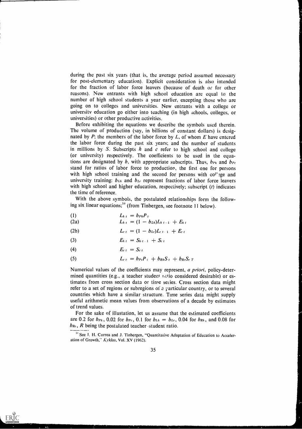
during the past six years (that is, the average period assumed necessaryfor post-elementary education). Explicit consideration is also intendedfor the fraction of labor force leavers (because of death of for otherreasons). New entrants with high school education are equal to thenumber of high school students a year earlier, excepting those who aregoing on to colleges and universities. New entrants with a college oruniversity education go either into teaching (in high .ichools, colleges, oruniversities) or other producfive activities.

Before exhibiting the equations we describe the symbols used therein.The volume of production (say, in billions of constant dollars) is desig-nated by P; the members of the labor force by L, of whom E have enteredthe labor force during the past six years; and the number of studentsin millions by S. Subscripts h and c refer to high school and college(or university) respectively. The coefficients to be used in the equa-tions are designated by b, with appropriate subscripts. Thus, brh and bp,stand for ratios of labor force to production, the first one for personswith high school training and the second for persons with col' ;ge anduniversity training: bLh and bLe represent fractions of labor force leaverswith high school and higher education, respectively; subscript (1) indicatesthe time of reference.

With the above symbols, the postulated relationships form the follow-ing six linear equations;" (from Tinbergen, see footnote 11 below).

(1) Lh t = bPhP,r(2a) Lh,t = (1 bLli)Lh r + Eh t

(2b) Lc,1 = (1 bl,c)Lc r t

(3) Eh t = Sh,t -1 ± Sc r

(4) Ec,t Sc t

(5) Lc = bPcP 4- bRhS t bRcSc T

Numerical values of the coefficients may represent, a priori, policy-deter-mined quantities (e.g., a teacher student t4ti0 considered desirable) or es-timates from cross section data or time sei ies. Cross section data mightrefer to a set of regions or subregions of a varticular country, or to severalcountries which have a similar structure. Time series data might supplyuseful arithmetic mean values from observations of a decade by estimatesof trend values.

For the sake of illustation, let us assume that the estimated coefficientsare 0.2 for bph, 0.02 for bp, 0.1 for bLh = Inc, 0.04 for bRh, and 0.08 forbRe, R being the postulated teacher-student ratio.

In See I. H. Correa and J. Tinbergen, "Quantitative Adaptation of Education to Acceler-ation of Growth,'" Kyldos, Vol. XV (1962).

35

.............

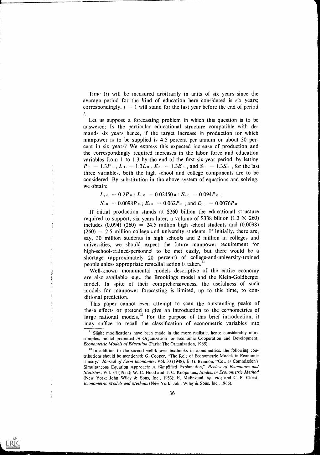
Time (1) will be nwasured arbitrarily in units of six years since theaverage period for the kind of education here considered is six years;correspondingly, 1 1 will stand for the last year before the end of period1.

Let us suppose a forecasting problem in which this question is to beanswered: Is the particular educational structure compatible with de-mands six years hence, if the target increase in production for whichmanpower is to be supplied is 4.5 percent per annum or about 30 per-cent in six years? We express this expected increase of production andthe correspondingly required increases in the labor force and educationvariables from 1 to 1.3 by the end of the first six-year period, by lettingP1 = 1.3P 0 , Li = 1.3L o , Li = 1.3E 0 , and S1 = 1.3S ; for the lastthree variables, both the high school and college components are to beconsidered. By substitution in the above system of equations and solving,we obtain:

Lh 0 = 0.2P0 ; L0 = 0.02450 0 ; Sh 0 = 0.094P 0 ;

S, 0 = 0.0098P0 ; Eh 0 = 0.062P 0 ; and LI, 0 = 0.0076P 0

If initial production stands at $260 billion the educational structurerequired to support, six years later, a volume of $338 billion (1.3 X 260)includes (0.094) (260) = 24.5 million high school students and (0.0098)(260) = 2.5 million college and university students. If initially, there are,say, 30 million students in high schools and 2 million in colleges anduniversities, we should expect the future manpower requirement forhigh-school-trained-personnel to be met easily, but there would be ashortage (approximately 20 percent) of college-and-university-trainedpeople unless appropriate remedial action is taken."

Well-known monumental models descriptive of the entire economyare also available e.g., the Brookings model and the Klein-Goldbergermodel. In spite of their comprehensiveness, the usefulness of suchmodels for manpower forecasting is limited, up to this time, to con-ditional prediction.

This paper cannot even attempt to scan the outstanding peaks ofthese efforts or pretend, to give an introduction to the econometrics oflarge national models:- For the purpose of this brief introduction, itmay suffice to recall the classification of econometric variables into

11 Slight modifications have been made in the more realistic, hence considerably morecomplex, model presented in Organization for Economic Cooperation and Development,Econometric Models of Education (Paris: The Organization, 1965).

12 In addition to the several well-known textbooks in econometrics, the following con-tributions should be mentioned: G. Cooper, "The Role of Econometric Models in EconomicTheory," Journal of Farm Econornics, Vol. 30 (1948); E. G. Bennion, "Cowles Commission'sSimultaneous Equation Approach: A Simplified Explanation," Review of Economics andStatistics, Vol. 34 (1952); W. C. Hood and T. C. Koopmans, Studies in Econometric Method(New York: John Wiley & Sons, Inc., 1953); E. Malinvaud, op. cit.; and C. F. Christ,Econometric Models and Methods (New York: John Wiley. & Sons, Inc., 1966).

36

endogenous ones (whose values it may be desired to predict), andexogenous ones postulated or assumed to be known a priori, and intojointly dependent (current endogenous) and predetermined (lagged en-dogenous and the exogenous) ones.

Many of the variables of interest to the manpower forecaster areusually treated as exogenous and thus are not convenient candidates formodel-based forecasting. Future government policies, union policies,propensities of individuals to enter or leave the labor force, familyformation, and attitudes toward ethnic groups are examples of variablesusually treated as exogenous." Some aspects relevant to manpowerforecasting are often absent altogether. Among these are "productionfunctions" for labor itselfthat is, the specification of variables and re-lationships describing education, training, and other forms of skill trans-fer.

Most of all, some of the major aggregative variables included inmodels may have been estimated via manpower forecasts. Thus we ex-pose ourselves, as earlier suggested, to the danger of circular reasoningwhen we use these variables in turn in manpower forecasting.

On the other hand, a closely related procedure, also structural innature, at this time seems to have much greater appeal to manpowerforecasters. The method alluded to goes under the name input-outputor interindustry analysis. In essence it is a form of multiple-entrynational accounting, or accounting for large geographic aggregates. Thisfamily of models has been of considerable interest to manpower analystsfrom its origin. At first glance the approach may resemble that of struc-tural models just-sketched. It, too, is based on interrelations presentedin a system of equations.

Subdividing the economy into many activities, e.g., industries or sec-tors, the input-output analysis presents an orderly tableau," an n-by-ngrid. The rows are the components of output (measured in dollars oftransactions) of a given industry or activity channeled into other in-dustries or activities, to which they become inputs and which are repre-sented by the columns. Each row-column intersection, or cell, lists theamount of the row activity entering the column activity as an input.Also attached to the table are several columns, including final demand(the so-called autonomous sectors), so that the tableau gives at oneglance a picture of the dollar transaction among industries according toinput and output and to final demand."

" See, however, the succinct contribution by S. Lebergott in J. S. Duesenberry, et al.,The 3rookings Quarterly Econometric Model of The United States (Amsterdam: North-Holland Publishing Co., 1965).

14la this aspect input-output traces back to the famous tableau economique of Quesney.

15 On the use of input-output analysis for forecasting, see the comprehensive presenta-tion by Clopper Almon, Jr., The American Economy to 1975 (New York: Harper & Row,Publishers, 1967).

37

By appropriate manipulation of this so-called transaction matrix,rived matrices or tables can be obtained that are of particular interest.

For example, the entries in the table may be expressed as percentagesof the respective column totals (the sector's output totals), indicat.ngthe purchasing sector's direct transfers or purchases from the produc-ing sector's per unit of output, say, per dollar (the so-called coefficientmatrix); from this matrix can be obLined a further Table showingthe direct as wei; as the indirect requirements placed on all industriesto support the delivery to final demand of a unit of output (say, onedollar), from each industry (the so-called inverse). Thus it becomespossible to "compute" rather than literally to trace step by step, theprimary, secondary, and higher order transactions which restth from,say, an increase in output of automobile production. This increase createsa direct demand for steeland many indirect ones for steel tooe.g., foramounts needed to support the very increase or steel production.

Once a table of direct and indirect input requirements has been com-puted (by solution of systems of simultaneous equations) it is easy enoughto translate these dollar amounts into manpower units. The resultingentries in the cells of the table may then be interpreted as reflectingdirect and indirect manpower requirements associated with a given out-put for a particular activity. This last-mentioned aspect of input-outputanalysis is of primary interest for manpower analysis and forecasting.A stipulated change somewhere in the economic strur-ture (perhaps anincrease in a specific demand) may be traced in its manpower aspectthroughout the system.

To convert the entries in a transaction matrix into a correspondingmanpower matrix, we must relate manpower and dollar variables in theseveral industries or activities. From this manpower matrix an inversecan be computed that shows direct and indirect manpower requirements,say, per $1 of final demand. This inverse makes it possible to analyzemanpower implications of proposed unemployment policies, of givenexport and import patterns, and of changes in the several componentsof final demand.'6 In addition to prediction, with the help of the inverse,we should recognize the forecasting of the input-output coefficients thern .

selves as a challenge to manpower analysis.So long as the economic structure as described by the coefficient

matrix remains reasonably stable, conditional prediction with its helpmay be safe enough. However, if the forecasting horizon In lig, thecoefficients themselves may change and a matrix more approv: - fora specified future date must first be provided.

Since the input-output coefficients of the manpower matrix indicate16

See, for instance, National Bureau of Economic Research, Input-Output Analysis:An Appraisal (Princeton: P:Anceton University Press, 1955), particularly the paper by W.Duane Evans and M. lioffenberg.

38

the manpower inputs (say, in terms of number of jobs) per unit of out-put, the factors likely to change the numerical values of these coefficientsneed to be explored. Among such factors, man-hours, productivity,and hours of work (since the measurement unit is a job) are particularlyimportant. They must be predicted for forecasting the economic struc-ture, the manpower inverse, and such.

Early work on employment oriented input-output analysis was under-taken under the sponsorship of the Bureau of Labor Statistics;11 the most

recent contribution in this direction was also made by the Bureau, al-though the basic input-output information used here was predicated onthe Department of Commerce's general input-output mati ix for 1958."

The manpower-projection scheme involves these phases when a

basic input-output table is alleady available:'9I. Total GNP prediction.2. Prediction of distribution of GNP over the various major compo-

nents of final demand.3. Prediction of the distribution of major demand components over

specific demand items.4. Application of these estimated dollar amounts to the inverse, that

is, multiplication of the inverse by each of the anticipated levels ofdemand. The resulting table gives in its cells the dollar amounts ofdirect and indirect requirements of the column industries that areto be satisfied by the row industries. (Intersection of column 15with row 6, for instance, would show the 15th industry's input fromindustry 6). Now these predicted output requirements nec.d to betranslated into corresponding manpower requirements.

5. The original input-output table is converted to an employment-requirement table by multiplication of the entries by per-dollaremployment estimates for each of the activities. Since per-dollaroutput requirements for manpower change with technology, factorsubstitution. etc.,2° the table obtained in this step must be amended

to incorporate such anticipated changes in its cells.6. The Bureau of Labor Statistics projects the employment-require-

ment table, taking accouni. of anticipated developments in labor

17 See J. Cornfield, W. Duane Evans, and M. Hoffenberg, "Full Employment Patterns,1950," Mon:hly Labor Review (February and March 1947).

18 See Survey of Current Business (November 1964 and September 1965)---papers by

M. R. Goldman, M. L. Marimont, B. N. Vaccara, and the National Income Division staff.

" For details see U. S. Bureau of Labor Statistics, Projections 1970, BLS Bulletin 1536

(Washington: 1967), and literature cited therein.

20 On measurement of labor input see W. Duane Evans, "Indexes of Labor Productivity

As a Partial Measure of Technological Change," Input-Ovum Relations, Proceedings of a

Conference on Inter-Industrial Relations Held at Driebergen, Holland (Leiden: H. E.Stenfert Kroese, N. V., 1953).

39

WOOMPm.~........

productivity- and man hours. Then predictions of the coefficientsin the table are made on the basis of intensive industry studies aswell as conjectures about technological changes, the length of thefuture working day, etc.-- Here and there, the coefficients observedfor leading establishments are imputed to an entire industry, onthe assumption that new technologies and factor-use patterns willeventually permeate the industry.

The forecasts of employment requirements derived by the multiplica-tion of the anticipated bill of goods with the corresponding entries in theemployment-requirement inverse (after the inverse, in turn, has beenprojected to the date of the desired forecast) are subject to various re-strictions. In addition to forecasting difficulties, there are difficultiesinherent in the input-output model itself. A fundamental identity is as-sumed for example, between product and activity. A related assumptionis product or out-put homogeneity (i.e., all outputs of a particular ac-.tivity or industry are essentially identical and interchangeable, dollarfor dollar). For a given time the coefficients of input to output are as-sumed constant; in other words, input-output ratios do not alter withchanging volume of output.

Thus far no attention has IA...41 given to the all-important question ofthe validity of information. In manpower or other socioeconomic fore-casting, the information available to the analyst is usually deficient insome degree.

Incompleteness of information is a typical situation, and much, if notall, of statistical method relates to the very problem of drawing inferencesfrom partial information. Modern sampling theory, for example, is usedfor estimating unknown characteristics of a population (the parameters)from statistics obtained from samples. If proper procedures are followedin gathering such sample data, then probability theory will point theway to estimates of sampling error and how to proceed from samplemeasures to population values for the particular population characteris-tics or the range within which this value is likely to be found. Otherthings being equal, the wider the acceptable range the higher our con-fidence that this range will contain the value of the characteristic. Inbivariate and multivariate situation, theory provides means for estimat-ing from sample data the "true" but unknown regression coefficients forthe population.

2' See Siegel (footnote 4, p. 7 in Chapter II) in Sar A. Levitan and Irving H. Siegel.Dimensions of Manpower Policy.

22 A procedure relying perhaps more heavily on formal techniques in the projection ofinput-output coefficients is described in a paper developed by the Department of AppliedEconomics, Un;versity of Cambridge, England, entitled "Input-Output Relationships,1954-1966" (distributed in the United States by MIT press, Cambridge, Mass., 1963).

40

4

The problem of prediction from time series is more complex. The stand-ard (parametric) approaches are based on assumptions hardly everrealized in typical manpower situations"' e.g., independenee of succes-sive observations, normality of distribution (-)f the residuals about a lineof regression, and unchanging variances over the observed time domain(so-called homoscedasticity).

Errors often result from incompleteness of the forecasting modelitself. Not all the relevant variables may be included the very purposeof model building. The form of the relationship may be oversimplifiedbeyond the permissible limit implieLly sought in a model. Errors ofmeasurement, the so-called errors of observations are presently thekind toward which classical statistical theory is directed, but error intime series observations is still not easy to handle. Heroic assumptionsmay be needed e.g., that our time series is in turn a sample from ahyperpopulation of all possible relevant time series. Still, it is importantto know the variances of the estimates where they are available, to com-pare the performance of different models and procedures and to providea eheck on likely usefulness and meaning of forecasts.

Of course, the specification of the model may itself be faulty. Atendency to include in a model as many relationships as can be obtainedis difficult to avoid; but if two or more of the predicting "independent"variables are actually interdependent, the validity of the system islimited. Thus two predictors that move in unison, that are highly in-

A glimpse into this problem is provided by Davis (footnote 17), Kendall and Stuart(footnote 4), Tintner, Goldberger, Johnston, and Yule and Kendall (footnotes 15 and16) with ample reference to more advanced literature. In addition to parametric methodsthat assume knowledge of the underlying probability distributions, distribution-free (so-called nonparametric) methods have been developed for the analyais of economic timeseries. Mar and Hotel ling were important early contributors; a not-too-technical presenta-tion may be found in M. G. Kendall, Rank Correlation Methods (London: Charles Grif-fin & Co., 1948) and in G. A. Ferguson, Nonparametric Trend Analysis (Mr,ntreal: McGillUniversity Press, 1965).

At this time still of minor importance for the manpower :orecaster are harmonicanalysis and spectral analysis. They are not discussed here. On the first, see Davis (foot-note 18 and M. G. Kendall, Contributions to the Study of Oscillatory Time Series (Cam-bridge, England: Cambridge University Press, 1946); on the latter, see J. Cunningham, "TheSpectral Analysis in Economic Time Series," Census Bureau Working Paper No. 14 (Wash-ington: 1963) and, for a more complete and more technical treatment, see W. J. Grangerand M. Hatanaka, Spectral Analysis of Economic Time Series (Princeton: Princeton Uni-versity Press, 1964).

The application of stochastic process models to economic time series has been discussedby H. 0. A. Wold, A Study in the Analysis of Stationary Time Series (Uppsala: Almqvist& Wiksells, 1938), and in the abundant recent literature see, for example, J. G. Kemenyand J. L. Snell, Finite Markov Chains (Princeton: D. Van Nostrand Co., Inc., 1960); andWold, Bibliography on Time Series and Stochastic Processes (Edinburgh; Oliver & Boyd,1965).

41

tercorrelated, amount to only one effective predictor. The macro varia-bles to be used in manpower forecasting (e.g., GNP, its major com-ponents and population) may all be strongly intercorrelated duringsustained periods of expansion. The resulting problem, called "multi-collinearity" by Frisch, introduces complexities and weakens the fore-casting capability of the model. Its presence should, at least, be rec-ognized by the manpower forecaster.

25

The difficult problems arising from the use of macro approaches thatdepend on highly aggregated information have recently evoked muchattention. Thiel's effective illucidation" has encouraged the explorationof other avenues. This quest has also been stimulated by practitioners'dissatisfaction with the state of statistical inference for the analysis ofeconomic time series. In the meantime, the investigation of the be-havior of complex systems has also received a potent fillip in the en-gineering and related fields from a computer application known assimulation. This technique was applied with reported success to a mis-

cellany of problems ranging from general management to transportation,traffic control, and military logistics."

The essentially stochastic nature of economic and behavioral relation-ships affecting manpower can .,he turned to advantage in simulation,which involves two operations:"8 construction of a model representing

the "real" process being considered; and experimentation with themodel via the computer, with a view to forecasting, testing, or design.The model is stated in mathematical terms but not, as earlier, to specify

a systt,n of contemporaneous equations to be solved together in orderobtain, say, predicted values of the variables.

The essential constituent elements of the model are the particular de-

" Ragnar Frisch, Statistical Confluence Analysis by Means of Complete RegressionSystems (Oslo: Universitets Økonomiske Institutt, 1934) proposed a useful graphic method(now unfashionable) called bunchmap analysis. See also O. Reierstil, Corzfluence Analysis

by Means of Instrumental Sets of Variables (Uppsala: Almqvist & Wiksells, 1945).25 On important problems facing the model builder, including the problems of statistical

inference in multiple regression, see E. F. Beach, Economic Models (New York: John

Wiley & Sons, Inc., 1957)." H. Theil, Linear Aggregation of Economic Relations (Amsterdam: Thrth-Holland

Publishing Company, 1954), addresses the conceptual obstacles to aggregation and shows

the difficulties that exist even when "perfect" aggregation is theoretically possible.

See, e.g., Reports of th2 System Simulation Symposium, American Institute of In-dustrial Engineers (New York: The Institute, 1957 and 1959).

28 See G. W. Morgenthaler, "The Theory and Application of Simulation in OperationsResearch," in R. L. Ackoff, ed., Progress in Operations Research, Vol. I (New York: John

Wiley & Sons, Inc., 1961), and an extensive bibliography on applications to other than thebehavioral sciences. For some examples of the application of simulation to business see

Proceedings on Simulation (New York: American Statistical Association, New York Area

Chapter, 1966).

42

cision-units say, individuals or firms -whose bdavior is to be studied,not the large economic aggregates underlying the economic macro modelsearlier described. Another departure from macro-modeling is in the pri-mary use of the computer to generate responses of the individual com-ponents.

Still in its early stages of development, sim..lation has been applied toforecasting in the behavioral fields especially in the general area ofdemography, which has many parallels to manpower analysis."9 A brieflisting of ingredients found in typical simulation indicates its nature anddata requirements:"

1. The "elements or components" e.g., individuals, households, firms,or goods.

2. The "attributes or variables" which may e divided intoa. "Responses" or "output variables" e.g., joining or not joining

the labor force, having a job, not earning an income, havingthree dependents, having children.

b. Factors influencing the behavior of the decision units other thantheir direct responsesinput invariables such as the season andthe responses (outputs) of other elements.

c. Status characteristics of the decision units e.g., age, sex, edu-cational achievement, income group.

3. Relationships necessary to prediction divisible into--a. Definitions or identities (e.g., the statement that income consists

of straight-time wage plus overtime wage plus nonwage income).b. The so-called operating characteristics (relationships which, for

a given element such as a person, tie item 2a to 2b and 2c);empirical or postulated, they are fed into the simulation tospecify how elements act or respond to stimuli.

Operating characteristics usually have to be stated in probabilisticrather than deterministic terms. For example, the probability that, in aspecific situation, a person of given sex, age and educational achievement(the status variables) will, during winter (an input variable reflecting theeffect of the seasonal component) join the construction industry (an out-put variable) is an operating characteristic. If age-and-sex-specific labor

29 See, e.g., M. C. Sheps and J. C. Riley, eds., Public Health and Population Change:Current Research Issues (Pittsburgh: University of Pittsburgh Press, 1965); Riley andSheps, "An Analytic Simulation Model of Human Reproduction with Demographic andBiological Components," Population Studies, Vol. 19 (1966); and M. Shubik, "Bibliographyon Simulation, Gaming, Artificial Intelligence and Allied Topics," Journal of the AmericcnStatistical Association, Vol. 55 (1960). Of particular interest to the mrnpower student isJ. Korbel's chapter on "A Labor-Force Model" in G. H. Orcutt et al., Micro Analysis ofSocioeconomic Systems: A Simulation Study (New York: Harper & Row, Publishers,1961).

" The presentation here follows closOy Orcutt, ibid, which also provides specific ex-amples. See especially pp. 15 ff.

43

force participation rates are available, estimating the correspondingprobabilities of joining the labor force may be relatively simple. In otherinstances, however, research may first have to be undertaken to providea reasonable probability estimate.

Since the model is descriptive of a historical process, it may be viewedas a sequence of equispaced cross sections or states, through time, per-haps one for each month. A state can be described by an appropriatetableau of probabilities corresponding to the operating characteristics.Applying the probabilities (often called transition probabilities) to thetableau of one state produces the tableau for the next.'" What charac-terizes simulation is the selection, according to these probabilities, of in-dividual elements (say, persons) for assignment to new locations ordestination in the next following state. Thus, given the probability of aparticular person's moving from unemployment in state t to employmentin state I + 1, his movement from Ito I + 1 can be simulated by a selec-tion mechanism that places a particular element chosen at random intoa new place with the desired probability. This selection, on the basis ofrandom choice (sometimes called the Monte Carlo method, a namegiven by von Neumann and S. Ulam) is undertaken by the computer atsuch an impressive speed that processes which would take years or gen-erations in real time can be collapsed to hours.

Starting with a sample of individuals or households, or with a cohortof women of, say, age 22, we may simulate the process of forward change.We may desire and attempt to modify the probabilities themselves asthe simulated process proceeds. The computer reads the original datainput for the initial state, updates with specific probabilities of transitionto state two, updates again, and so forth.32

Problems of sampling or statistical inference are difficult enough forempirical time series; they are, as yet little explored for input-outputanalysis and simulation. The manpower forecaster looking for some wayto improve his forecasts, to attach to them measures of reliability, shouldconsider if the forecasting method itself can be improved? As in theproof of Cervantes' pudding, comparison of forecast and actual outcome(the "realization") plays an important role. For such comparative evalua-tion Theil has proposed an intriguing yet simple technique.43

This method, applicable to manpower forecasts, systematically com-pares a predicted percentage change, PT (where T refers to the particu-

For an application of transition probabilities to a labor force problem, see I. Blumcn,M. Kogen and P. J. McCarthy, The Industrial Mobility of Labor as a Probability Process(Ithaca: Cornell University, 1955).

3 2 To facilitate communication with the computer, special-purpose languages have beendevised, e.g., Simscript. Of particular interest to labor force type of simulation is ProgramSimulate, Revision AB, by C. C. Holt et al. (Madison: University of Wisconsin, 1965).

3,1 H. Theil, Applied Economic Forecasting (Amsterdam: North-Holland Publishing Co.,1966), and "Who Forecasts Best?" International Economic Papers, No. 5 (1955).

44

lar time, say, year), and the actually realized change, AT. The expression

is an average measure of the magnitude of total discrep-

ancy. Relating this term to the average of squared realized changes,:LA 2 AT)7. Theil obtained U2 -- A measure of discrepancies,

N IATU is called the inequality coefficient. A valuable property of this meas-ure is that, like variance, it can be decomposed into three components,each indicative of a particular source of errors. The three components are:

1. (P A)2, the error in central tendencies;2. (0-p , the error of unequal varititions; and3. 2(1 r)apaa , where r measures the correlation between predicted

and actually observed changes, and 0- is the standard deviation.Expressing these three components as fractions of the total discrep-

(X(PT 7.)2 )ancy A we obtain three fractions; Uni, LI, and Um, the

bias fraction indicates the degree of discrepancy between average pre-dicted and average actually observes values. LI, the variance fraction,suggests the presence of residual cycles and fluctuations in the deviationsof predictions from realizations, (the forecasting procedure may not takeadequate account of business cycles or other cyclical features of the proc-ess). vanishes only if average predicted changes equal actually ob-served changes--a property expected from a good forecasting procedure,since the forecast should be correct "at least on the average." Thus, ifIr is relatively large, the forecasting procedure would seem deficient;and adjustments and improvements would be called for. A relativelylarge LI should alert the forecaster to the possibility that cyclical forceshave been overlooked.

Lie, the "covariance" fraction, characterizes a more abstract aspectof the relation between forecast tnii actually realized changes. SinceUm + U8 + U1 1, U is the residual component; it represents error,due to what Theil calls incomplete criation. The forecaster can dolittle, if anything about them."'

Another test criterion for prediction schemes is Wold's Janus coeffi-cient.3') This measure, analogous to the F ratio (named after R. A.Fisher) is defined as the ratio of (a) the mean squared discrepancy be-

' On inequality coefficients, see Theil, Applied Economic Forecasting op. cit., and hisEconomic Forecasts and Policy (1st ed.; Anbterdam: North-Holland Publishing Co., 1938).Also of interest is Thiel's simple graphie method (the so-ealled predietion-realization dia-grams) which at a glance reveals the extent to which the forecasting procedures have re-sulted in overestimation or inderestimation, and their sensitivity in anticipating turningpoints.

A. Gadd and H. 0. A. Wold, "The Janus Coefficient: A Measure for the Accuracy ofPrediction," in H. 0. A. Wold, ed., Ecomnnetric Model Building (Amsterdam: North-Hol-land Publishing Co., 1964). The reference to Janus indieates that the measure looks forwardover the prediction horizon and backward over the sample period.

45

tween projected and (later) observed values to (b) the mean squareddiscrepancy between estimates that would have been obtained by ap-plication of the model to the sample period itself and the correspondingactual observations. In algebraic terms,

E (Pr AT)T N I

T N

(Er A 7')T

Here P again refers to the predicted values, E to the estimates whichwould have been obtained by application of the model to past data,A to the actual values, and T = 1, 2, N, N 1, N M, totime, say, in years or months. The first N observations refer to thesample (the observerl 'ast) on which the prediction model is based, andthe next M intervals refer to the prediction horizon. The measure can ofcourse be obtained only after accumulation of experience with the fore-casting model during the M periods.

As Wold himself points out, J is an indicator of the relative size of thediscrepancy between P and A It thus does not appraise the particularforecasting procedure for sensitivity to turning points or for ability toanticipate them accurately.

VI. Retrospect and ProspectManpower forecasts are, like other statistical measures and estimates,answers to particular questions,' so there are many varieties of forecastsobtainable by many techniques. The alternatives would appear evengreater had we included the methods adaptable to manpower forecastingbut not actually so employed. Thus, the manpower forecaster reallyworks from an embarrassment of riches. He therefore must often chooseamong different methods and interpret competitive forecasts. We nowreview the gamut of forecasting approaches, attempting to sharpen thereader's appreciation and comprehension of them by an exposition interms of dichotomies, which in reality represent only the extreme pointsof continua.

Short-Term Versus Long-Term ForecastingAlthough the distinction between short-term and long-term forecasts

is common, it is among the less informative ones. Manpower forecastingwhen concerned with a variable that is a simple function of population,frequently focusses on a longer forecasting range or horizon than does the

See R. A. Lester, Manpower Planning in a Free Society (Princeton: Princeton Univer-sity Press, 1966).

46

prediction of other important economic variables. If, for instance, a man-power component is to be forecast which strongly depends on the "closedactive populatim" i.e., the population that is between ages A and A. aridnot subject to change by migration, a relatively long forecasting horizonis generally permissible. For example, if the closed active population in-cludes all persons bet%een the ages of 15 and 65, a forecast looking 15years hence would seem to be safer than for nearly any other economicvariable independent of or less dependent on, population size. But evensuch a forecast involving persons already alive, involves restrictive as-sumptions, a major one being the stability of the age-specific death ratesover the next A years.

In general, however, long-term forecasts are less certain of realizationthan short-term ones. For one thing, assumptions of stability in trend, inratios to other variables, etc., become more and more tenuous the longerthe period anticipated. Furthermore, the chance of major structuralalterations or of a sudden change in an exogenous variable- increaseswith the time horizon. If a forecast is made for a year 10 or 15 yearshence, the secular trend need be considered, but not the variations andcycles shorter than 10 or 15 years.

A short-term forecast, say, for six months hence, does require knowl-edge about short-term (in this case intra-annual) fiuctations. The analysisof seasonal variations and their inclusion in the projection is vital.

Stochastic Versus Deterministic Approach

The term "stochastic," originated with James Bernoulli in 1713.3 Inits present meaning it has been in wider use only for a relatively shorttime, having been reintroduced by von Borthiewicz and Tschuprow.4 Itis now frequently employed in economics and elsewhere to characterizeerrors of observation and other sources of variability about the under-lying "true" value that is to be estimated. In a stochastic relationshipbetween two or more variables an unequivocal sharply defined relation-ship is not postulated as in the "deterministic" case. A stochastic variablemay be described in terms of a probability distribution. Empirical eco-nomic relations are, as a rule, stochastic relations.

Nonstochastic, i.e., deterministic, approaches are typically used in man-power forecasting because of their relative simplicity or for lack of suffi-cient and appropriate estimates. We usually assume a functional re-

" Exogenous variables. as opposed to endogenous ones. are variables independent of theeconomy; many acts by governments are of this nature. Which specific variables are to betreated as exogenous and which as endogenous depends of course on the forecasting methodor model used.

3 Ars Coqjectandi (Basel: Impensis Thiirnisiorum. fratrum. 1713).4 A. A. Tschuprow, "Ziele und Wege der Stochastischen Grundlegung der Statistischan

Theorie, "Nordisk StalArisk Tidarili," Vol. 3 (StockhGlm: 1924).

47

lationship for what we know to be a stochastic one. Although nopracticable solution to the stochastic problem may be available, it is

important to keep in mind the inherently stochastic character of fore-casting from empirical data. Neglect may result in forecasting-blundersof considerable magnitude.

Potht Versus Interval Forecasts

Forecasting of an empirical stochastic process will result, not in asingle value of the predicted variable, but in a distribution of predictionswith varying probabilities. As a rule, therefore, we can forecast withgreater assurance in terms of a range of values than in terms of a singlepoint.

Even in nonstochastic procedures, the validity of the forecast cFn pre-sumably be improved if a range is substituted for a point. Instead of asimple forecast we may with greate1 assurance provide an upper andlower limit or provide several forecasts with slightly different assumptions.The Census Bureau's alternative populati:.ii forecasts illustrate this ap-proach.

It is the user of predictions rather than the forecasting model thatoften has to be blamed for apparent shortcomings of the latter. Enor-mous pressure is placed on forecasters to provide point estimates, tomake one forecast only. The elementary urge of the pragmatic man ofaction is to obtain a unique figure. An aversion to interval estimates,however, does not speak well for the sophistication of the statistics user.

Unconditional Versus Conditional Forecasts

An unconditional forecast is aot contingent on the realization of aspecific condition. Fore-mst of the size of the male labor force by meansof a trend fitted to, say, the male labor force figures for the past six yearsis unconditional if no additional qualifications are introduced.

A great many manpower forecasts are conditional, although the userdoes not always ascertain what the conditions are. Furthermore, themaker of forecasts does not always bother to spell out the major im-plicit conditions that he really accepts for his procedure. Examples ofwell-qualified conditional forecasts are the Census Bureau's populationforecasts.' Practically all economic forecasts are conditional in that they

assume certain stabilities on which there could be considerable disagree-ment. Few forecasts, however, are adequately qualified,6 and full quali-fication is exceedingly difficult if not impossible.

For other examples, see H. Theil, Applied Economic Forecasting (Amsterdam: North-

Holland Publishing Co., 1966).This fact was recently stressed by W. Lee Hansen, "Labor Force and Occupational

Projections," in Gerald G. Somers, ed., P. oceedings of the Eighteenth Annual Winter Meet.

ing qf the Industrial Relations Research Association (Madison: The Association, 1966).

48

Conditional forecasts based on clearly stated major assumptions arevery useful. They help to realize that important premises may not ac-tually be met; they help us to trace the implications of a policy under

consideration. Alternative conditional forecasts permit a comparisonof likely results of competitive assumptions or decisions.

First-Order Versus Higher-Order Forecasts

A forecast is usually treated as a first-order forecast as if it were "neu-tral" with respect to the future course of the event predicted. Tile fore-cast itself, however, might affect the future value of the predicted vari-

able. In many situations, in the social sciences, as elsewhere, a forecast

may be "adaptive" and the process under consideration may be subject

to prediction-feedback. It is also conceivable that higher than second-

order effects may have to be considered, for the expected or estimatedreaction to a forecast could further modify the ultimate outcome. Cropestimations and stock market forecasts have early been recognized asgiving rise to such higher-order effects.

In microeconomic situations, second-order forecasts in the above sense

are frequently encountered!' On macro levels they will be encountered

when the variable in question is a subject of active and deliberate policy.Much manpower forecasting, therefore, should be treated as of a higherorder, especially when the adaptive period, e.g., the period for trainingskilled and specialized manpower, is a long one. Unless higher order con-siderations are incorporated in the forecasting procedure, first-order pre-dictions by themselves may actually frustrate the intended policy; theymay, for instance, result in more violent fluctuations and distortionsthan in the absence of prediction.

Logically related to this issue is so-called "teleological" forecasting.9

Such forecasting relates not to what is likely to happen in the future but

to targets that should be achieved. Teleological macro prediction poses

a problem that is pertinent to the United States, as well as to centrallyplanned economies and the so-called developing countries. In the evalua-

tion of structural unemployment, for example, it is useful to predictfuture skill needs to meet the "target" of full employment. On the microlevel, teleological forecasting is encountered, for example, in the applica-

tion of linear programming techniques.If manpower forecasting is used as a diagnostic device, and if diag-

nosis and therapeutics are responsibilities of the same person or or-

In more recent sociological literature one finds the term "self-fulfilling prediction" to

describe a similar effect.Theil. op. cit.. proposes the term "anticipations" if the forecaster has no direct control

over what he predicts. and the term "plan" if the forecast variable "is directly controlled by

the forecaster himself."See R. K. Srivastava icting Manpower Demand (Government of' India. Direc-

torate of Manpower. Ministry Home Affairs. 1964).

49

ganization, the anticipated effect of therapeutics cannot be ignored. Someof the implications are only gradually being recognized. and we are farfrom finding satisfactory solutions." In the manpower field, as in others,the problem is complicated by our limited ability to influence the future.Even where government policy may be expected to alter effectively theresults based On a "neutral" forecast, only a part of what is predictedmay be subject to corrective therapeutic action ,:Jrecasting in such in-stances would have to proceed along two lines, distinguishing what isamenable to control via feedback from what is autonomous and un-controllable, yet not necessarily random.

Manpower forecasting schemes typically assume the relative stabilityof the underlying socioeconomic structure. For the usual predictionhorizon, this premise does not seem unreasonable. However, the ex-panding scope of manpower policies and the momentum of technologicalchange compress the scale of process time as compared with historicaltime. What once was assumed fixed will itself have to be forecast. Thus,we shall have ensuing need to forecast the changing future shape of theskill and occupational structure on both the "supply" F,ide (as affected byeducation and training) and the "demand" side (as affected by alterna-tives of skill requirements)."

Formal prediction usually avoids the difficult issue of interstructuralversus intrastructural change. No structural change is the usually stipu-lated condition, or such change is relegated to the exogenous part of themodel. Yet the manpower forecaster must face the issue in one way oranother. In the physical and life sciences, it is possible on occasion tomodelize extensive structural change,L but much too little is knownabout socioeconomic subject matter to procede in comfort along "ob-jective" lines.

We come now to the much vaguer and highly subjective areas of con-jecture and guess, if not augury.

"} See, for instance, Bertrand de Jouvenel, The Art of Conjecture (New York: BasicBooks, Inc., Publishers, 1967); also H. 0. A. Wold, in Study Week on the Econometric Ap-proach to Development Planning (Amsterdam: North-Holland Publishing Co., 1965).

" For projections of scientific and engineering manpower aspects in this country, wherethe problem of anticipating technological change is fundamental, see the Bureau of LaborStatistics study, The Long-Range Demand for Scientists and Technical Personnel, NSF61-65; D. M. Black and G. J. Stigler, The Demand and Supply of Scientific Personnel (NewYork: National Bureau of Economic Research, 1957). For the importance of technologicalfactors in estimating future occupational composition in general, see Bureau of LaborStatistics, Special Labor Force Report No. 28 (1963); and R. A. Gordon, ed., Long-TermManpower Projections (Berkeley: Institute of Industrial Relations, University of California,1965).

12 For an imaginative and not-too-technical exposition in a particular instance, see D'ArcyWentworth Thompson, On Growth and Form (2nd ed.; Cambridge, England: CambridgeUniversity Press, 1959).

50

*ogmmfINa.tygTiNr**

During the last few years efforts have been made to sharpen our in-sights into the future:'"

1. The most broadly gauge] approach is that of the French organiza-tion, the Futuribles, .,.nder the direction of Bertrand de Jouvenel."

2. In the United States the Department of li.Lr:rise and the RandCorporation'' have sought to anticipate tr, tical developments;the latter organization has employed the a LAphi methodfor establishing a concensus of expert or..

3. Industry has followed these develop .!, perimentingwith additional forecasting techniques i. major al-teration of the technological structure."

These attacks on a most significant problei3 tL impressive,

not because of their methodological resuits f-;ut . their couragein facing a very difficult and importan' plot .n.. It sei s ,o concludethat these endeavors have as yet not extended beyond tiie r ge of thestructural certainties, beyond the range in which "our future cataintiesare features inherent in an order in which we have confidence"."

The preplexing difficulties of the task of solving what appears a vc it-

able riddle of the sphynx reach deep into the epistemological foundationsof economics and the behavioral sciences. Hence it would seem that themore conventional manpower forecasting methods, sometimes termednaive, should be improved rather than discarded; they are all we reallyhave. Bold attempts, however, should be encouraged. They will, if nothingelse, generate new hypotheses that require confrontation and testing.

13 Among individuals see, e.g., J. von Neumann "Can We Survive Technology?" Fortune,LI (1955); Harrison Brown, et al., The Next Hundred Years (New York: The Viking Press,1958); T. H. Gordon, The Future (New York: St. Martin's Pres,i, Inc., 1965); and I. J.Good, ed., The Scientist Speculates (New York: Basic Books, Inc., Publishers, 1962).

" See the series Futuribles of the bulletin Sedeis (Paris).

Army Research Office, Long-Range Technological Forecast (Washington: 1963); andRAND Corporation, publications P-3063 and P-2986 (Santa Monica). For a broadgaugedsynopsis see Erich Jantsch., Techiwlogical Forecasting in Perspective (Paris: Organizationfor Economic Co-operation ond Development, 1967).

In addition to the just-cited RAND papers, see also 0. Helmer, Social Technology

(New York: Basic Books, Inc., Pt:;Ilishers, 1966), especially his contribution jointly with

.1". H. Gordon discussing the specific application of the Delphi method. Among the in-dustries are General Electric Corporation, Westinghouse Electric Corporation, TRW In-corporated (whose forecasting techrnque, Probe, is reminiscent of the Delphi method) and

the Hudson Institute (whost, zoncern i:, in the general area of international economicrelations).

17 de Jouvenel, op. cit.

Documents

Some of the problems and techniques involved in manpower ... · Methods for Manpower ... Some of the problems and techniques involved in manpower forecasting ... Sometimes "prediction"