Some novel models of distributions over the unit square

Journal of Statistical Planning andInference 109 (2003) 3–30

www.elsevier.com/locate/jspi

Some novel models of distributionsover the unit square

Norman Johnsona, Samuel Kotzb;∗aDepartment of Statistics, University of North Carolina, Chapel Hill, NC 27599-3260, USAbDepartment of Engineering Management, The George Washington University, Washington,

DC 20052, USA

This paper is dedicated to Professor C.R. Rao on the occasion of his 80th birthday

Abstract

Motivated by the work of Borkowf et al. (Biometrics 53 (1997) 1054), properties of (depen-dent) bivariate distributions obtained by piecewise modi5cations of uniform distributions overthe unit square ([0; 1]2) are studied, with special reference to cases of uncorrelatedness betweendependent variables. Moments of the distributions are derived and values of several classicaldependence indices are obtained and discussed.c© 2002 Published by Elsevier Science B.V.

Keywords: Bivariate uniform distribution; Correlation; Moments; Schweizer–Wol< dependence index

1. Introduction

In the course of studying the literature on statistical distributions during recent yearswe have been constantly amazed at the variety of distributions that have been lyingaround, little noticed, for many years, but are now 5nding speci5c (sometimes unex-pected) practical applications. Quite recently (Johnson and Kotz, 1999) we encounteredan application in the theory of stock market prices, leading to generalizations of tri-angular distributions and posing some challenging problems in estimation procedures.The present paper is motivated by the use of piecewise modi5cations of the uniformdistribution over the unit square, [0; 1]2, as a model in simulating sampling distributionsof statistics based on cell counts arranged in two-way contingency tables, by Borkowfet al. (1997)— referred to later as BGCG.

These distributions are of interest since they provide inter alia natural, transparentexamples wherein zero correlation does not imply independence. We discuss some

∗ Corresponding author.

0378-3758/02/$ - see front matter c© 2002 Published by Elsevier Science B.V.PII: S0378 -3758(02)00292 -6

4 N. Johnson, S. Kotz / Journal of Statistical Planning and Inference 109 (2003) 3–30

simple extensions of these distributions, sharing this property. Our investigations arelimited to continuous distributions, evaluation of some joint moments and measures ofdeparture from uniformity, notably the so-called Schweizer–Wol< measure of depen-dence, (Schweizer and Wol<, 1981) which, for uniformly distributed random variablesX1 and X2 over the unit square [0; 1]2, is of the form:

� = 12∫ 1

0

∫ 1

0|FX (x) − x1x2| dx1 dx2 (1.1)

(see also Schweizer, 1991; Feuerverger, 1993). Here FX (x)=Pr[⋂2j=1 (Xj6 xj)] is the

joint cumulative distribution function (cdf) of X1 and X2. This measure was plannedas a measure of dependence in cases where both marginal distributions are uniform.If the distribution is uniform over the unit square ([0; 1]2) then the joint probabilitydensity function (pdf) of X1 and X2 is

fX (x) = fX1 ; X2 (x1; x2) =

1 for⋂2

j=1(06 xj6 1);

0 elsewhere:(1.2)

For this case FX (x) = x1x2 for⋂2j=1 (06 xj6 1) and consequently � = 0.

When the condition of uniform marginal distributions is not satis5ed, the criterionmeasures a combination of e<ects of dependence and other departures from uniformity.The former, alone, could be measured by the index

12∫ 1

0

∫ 1

0|FX (x) − FX1 (x1)FX2 (x2)| dx1 dx2: (1.3)

The coeHcient 12 in (1.1) is chosen because for any copula (a multivariate prob-ability distribution function with uniform univariate marginals on the interval [0; 1])corresponding to FX (x); C(x1; x2) say,

12∫ 1

0

∫ 1

0|C(x1; x2) − x1x2| dx1 dx26 1:

(Compare with the much earlier dependence index suggested by Hoe<ding (1940):2 = 90

∫ 10

∫ 10 (FX (x1; x2) − x1x2)2 dx1 dx2, which did not receive much attention in

the literature.) Indeed, the double integral∫ 1

0

∫ 10 |min(x1; x2) − x1x2| dx1 dx2 = 1

12 forthe most-dependent copula, with C(x1; x2) = min(x1; x2). Thus �= 1 under this settingmeans that X1 and X2 are strictly monotonically functionally related. Note that C(x1; x2)= FX (F−1

1 (x1); F−12 (x2)) where Fi(xi), are the marginal c.d.fs of Xi; i = 1; 2. Also

recall that for bivariate uniform distributions on [0; 1]2 with independent marginalsC(x1; x2) = x1x2.

In our applications, however, FX (x) may not represent a copula of any distribution(namely the marginal distributions may not be uniform), and the value of � may indeedexceed 1, as the example below indicates. We may have both dependence and otherdeviations from bivariate uniformity.

N. Johnson, S. Kotz / Journal of Statistical Planning and Inference 109 (2003) 3–30 5

Fig. 1. Simple two-valued modi5ed uniform square distribution.

Consider X1 and X2 with joint distribution as indicated in Fig. 1 where the jointdensity in the blank rectangle is 0 and, in the black rectangle, it is 2. (In this casethe marginal of X1 is not uniform, though X2 does have a uniform distribution.) Herewe have∫ 1

0

∫ 1

0|FX (x) − x1x2 | dx1 dx2 = 2

∫ 1

0

∫ 1=2

0x1x2 dx1 dx2

= 2( 12 × 12){ 1

2 × ( 12 )2} = 1

8 ;

whence � = 1:5.

2. Modi�ed distributions on the unit square

We will discuss some of the consequences when the probability mass is redistributedover the unit square, while retaining a piecewise uniform structure. We shall be primar-ily concerned with distributions for which X1 and X2 have zero correlation, with specialreference to the e<ects of these kinds of departure from uniformity and independenceon measures of dependence.

As indicated in Section 1, the distributions discussed in this section do not haveboth marginal distributions uniform, but in all cases the correlation coeHcient is zero.In all cases, in fact, the conditional distribution of at least one variable, given anyspeci5c value of the other, is symmetrical and consequently has expected value 1

2 . Forexample, if

E[X1|X2 = x2] = 12 for all x2 (0¡x2¡ 1)

then

E[X1] = 12 and E[X1X2] = 1

2 E[X2] = E[X1]E[X2];


Fig. 2. Single nicked square distribution.

Fig. 3. Generalized nicked square distribution.

so

cov(X1; X2) = 0:

See Fig. 2 for the so-called (single) nicked square distribution originally proposed byBGCG (1997); a generalization is presented in Fig. 3, while Fig. 4 depicts the newlyintroduced (single) “notched square” distribution.

In Fig. 3, to ensure that the marginal distribution of X2 is uniform, we takeP1 = 1; P2 = (a+ b)=b [P1 = 1; P2 = 2 if a= b].

Further possibilities are set out below, in Figs. 5 and 6 (double and quadruple‘nicked’) and Figs. 7 and 8 (double and quadruple “notched”). We will use the


Fig. 4. Single notched square distribution.

Fig. 5. Double nicked square distribution.

Fig. 6. Quadruple nicked square distribution.


Fig. 7. Double notched square distribution.

Fig. 8. Quadruple notched square distribution.

following abbreviations for these “Square” distributions:

Nicked Notched

Single SNiS SNoSDouble DNiS DNoSQuadruple QNiS QNoS

Before concluding this catalog of distributions, we note that unless the modi5eddistribution has both marginal distributions uniform, this distribution is not appropriateto use as a possible alternative to independence if X1 and X2 are themselves cdfsof continuous variables (say Y1; Y2) and are to be used in simulations of alternativejoint distributions for calculating power of tests of independence. This is because thealternatives then could rePect changes from hypothesized distributions of Y1 and/or Y2,as well as dependencies.


Section 3 presents joint moments of the distributions introduced above; Section 4presents values of � for them. Section 5 includes some comments on these results, andbriePy investigates some further possible modi5cations.

Rather subtle (though elementary) mathematical techniques employed in deriving theresults in Sections 3 and 4 are described in the appendix.

3. Moments

In all the cases described in Section 2, the conditional distributions of X1, givenX2 = x2, and of X2, given X1 = x1, are symmetrical, for all 0¡x1¡ 1; 0¡x2¡ 1. 1

This means that, for nonnegative integer values of r1; r2

E[(Xi − 12 )ri |(X3−i = x3−i)] = 0 if ri is odd (i = 1; 2):

Hence

E[(X1 − 12 )r1 (X2 − 1

2 )r2 ] = 0 if either r1 or r2 is odd: (3.1)

If both r1 and r2 are even, then for the uniform distribution over the unit square,

�r1 ;r2 = E[(X1 − 12 )r1 (X2 − 1

2 )r2 ] = E[(X1 − 12 )r1 ]E[(X2 − 1

2 )r2 ]

= (r1 + 1)−12−r1 (r2 + 1)−12−r2

= (r1 + 1)−1(r2 + 1)−12−r1−r2 : (3.2)

For the (generalized) single nicked square (SNiS) distribution (Fig. 3)

E[(X1 − 12 )r1 |X2 = x2]

=

(r1 + 1)−12−r1 (h6 x26 1);

(r1 + 1)−12−r1 + 2(r1 + 1)−1

×b−1a(a+ b){(a+ b)r1 − ar1} (06 x26 h);

(3.3)

whence

�r1 ;r2 = (r1 + 1)−1(r2 + 1)−1[2−r1−r2

+ 2b−1a(a+ b){(a+ b)r1 − ar1}{( 12 )r2+1 − ( 1

2 − h)r2+1}]

= (r1 + 1)−1(r2 + 1)−1[2−r1−r2 + 2w(r1; r2; a; b)]; (3.4)

where

w(r1; r2; a; b) = b−1a(a+ b){(a+ b)r1 − ar1}{( 12 )r2+1 − ( 1

2 − h)r2+1}: (3.5)

when a= b (and so P2 = 2),

w(r1; r2; a; b) = 2(2r1 − 1)ar1+1{( 12 )r2+1 − ( 1

2 − h)r2+1}: (3.6)

1 For the double and quadruple distributions, this is also true of the conditional distributions of X2, givenX1 = x1, for all 0¡x1 ¡ 1.


For double nicked square (DNiS) distributions (Fig. 5)

�r1 ;r2 = (r1 + 1)−1(r2 + 1)−1{2−r1−r2 + 4w(r1; r2; a; b)}: (3.7)

For quadruple nicked square (QNiS) distributions (Fig. 6)

�r1 ;r2 = (r1 + 1)−1(r2 + 1)−1[2−r1−r2 + 4{w(r1; r2; a; b) + w(r2; r1; a; b)}]: (3.8)

For single notched square (SNoS) distributions (Fig. 4)

E[(X1 − 12 )r1 |X2 = x2] =

(r1 + 1)−12−r1 (h6 x26 1);

2(r1 + 1)−1[( 12 )r1+1 − (1 − x2

h )r1+1{(a+ b)r1+1

− a+bb ((a+ b)r1+1 − ar1+1)}]

= (r1 + 1)−12−r2

+2(r1 + 1)−1(1 − x2h )r1+1b−1a(a+ b)

×{(a+ b)r1 − ar1};

(3.9)

whence

�r1 ;r2 = (r1 + 1)−1(r2 + 1)−12−r1−r2 + 2(r1 + 1)−1b−1a(a+ b){(a+ b)r1 − ar1}

×∫ h

0

(1 − x2

h

)r1+1 (x2 − 1

2

)r2 dx2

= (r1 + 1)−1(r2 + 1)−12−r1−r2 + 2(r1 + 1)−1b−1a(a+ b){(a+ b)r1 − ar1}

× 2−r2hr2∑j=0

(−1)j(r2

j

)(2h)jB(j + 1; r1 + 2)

= (r1 + 1)−1(r2 + 1)−12−r1−r2 + 2(r1 + 1)−1u(r1; r2; a; b); (3.10)

where u(r1; r2; a; b) = b−1a{(a+ b)r1 − ar1}

×2−r2hr2∑j=0

(−1)j(r2

j

)(2h)jB(j + 1; r1 + 2) (3.11)

and B(�1; �2) =∫ 1

0 t�1−1(1 − t)�2−1 dt is the complete beta-function.

If a= b (so P2 = 2)

u(r1; r2; a; a) = ar1 (2r1 − 1)2−r2hr2∑j=0

(−1)j(r2

j

)(2h)jB(j + 1; r1 + 2): (3.12)

For double notched square (DNoS) distributions (Fig. 7)

�r1 ;r2 = (r1 + 1)−1(r2 + 1)−12−r1−r2 + 4(r1 + 1)−1u(r1; r2; a; b): (3.13)


For quadruple notched square (QNoS) distributions (Fig. 8)

�r1 ;r2 = (r1 + 1)−1(r2 + 1)−12−r1−r2

+4(r1 + 1)−1{u(r1; r2; a; b) + u(r2; r1; a; b)}: (3.14)

It is easily deduced from these formulas that correlations are zero in all the 6 casescited above.

We note that for quadruple (nicked and notched) distributions, we should have:

0¡h+ 2a¡ 12 :

For double and quadruple cases

0¡h¡ 12

and, of course,

0¡h¡ 1

for single cases.

4. Measures of dependence and departures from uniformity

For distributions on the unit square

� = 12∫ 1

0

∫ 1

0|FX (x) − x1x2| dx1 dx2: (1.1 bis)

Values of � for the six distributions introduced in this paper are presented below. Acritical discussion of the usefulness of � as a measure of departures from uniformity,with brief studies of a few other distributions on [0; 1]2 and related dependence indicesfollows.

Details of the calculation of � are given in the appendix. We note here that calcu-lation of∫ 1

0

∫ 1

0|FX (x) − x1x2| dx1 dx2 (4.1)

is facilitated, for the distributions considered in this paper, by the fact that they areall piecewise uniform, so that the excess density (fX (x)− 1) is constant over each ofseveral regions formed by subdividing the unit square.

In this section, we will take a = b (and P2 = 2; P1 = 1; 0¡a6 14 ). This means

that the excess density is equal to 1 for regions marked black, zero for regions withcross-hatching, and −1 for regions left blank.

For SNiS distributions (Fig. 3).

� = 24a2h(1 − 12h): (4.2)

The maximum value (� = 34 ) is attained for h = 1 with a = 1

4 , which leads to thecon5guration in which the excess density equals 1 in the two rectangles with thevertices (0; 0); (0; 1); ( 1

4 ; 1); ( 14 ; 0); ( 3

4 ; 0); ( 34 ; 1); (1; 1) and (1; 0) and the excess density

of −1 in the complementary region of the unit square.


For DNiS distributions (Fig. 5)

� = 24a2h: (4.3)

The maximum value of 34 is attained for a= 1

4 and h= 12 .

For QNiS distributions (Fig. 6)

� = 48a2h(1 − 43a): (4.4)

For SNoS distributions (Fig. 2)

� = 8a2h(1 − 14h): (4.5)

For DNoS distributions (Fig. 7)

� = 8a2h: (4.6)

Compare (4.5) and (4.6) with the DNiS case (4.3) above. The values of � in theNoS cases are three times smaller than the corresponding values in the nicked cases.For QNoS distributions (Fig. 8)

� = 16a2h(1 − 12a): (4.7)

The � index does rePect dependence as indeed originally intended but also deviationfrom uniformity in these distributions even though they have zero correlation. Themagnitude of � does increase with greater irregularity (areas of departure (±1) fromuniform density), progressing though single, double and quadruple nicked and notchedsquare distributions.

However, there are (not surprisingly) some disturbing features associated with theuse of the index in these situations (in which marginal uniformity does not hold).If Fig. 2 (SNiS) is turned upside-down, so that the ‘nick’ is at the top (x2 = 1) ofthe square, instead of on the x1-axis, the value of � changes from 24a2h(1 − 1

2h) to12a2h2! (The value of � is still 24a2h(1 − 1

2h) if the nick is moved to the left-handside (x2-axis) of the square, but it is 12a2h2 if the nick is moved to the right-handside (x1 = 1) of the square).

Further, if the regions marked black (P2 = 2) are each moved out from a¡ |x1 − 12 |

¡ 2a to |x1 − 12 |¡ 3a (see Fig. 9), the value of � doubles to 48a2h(1 − 1

2h). (Withsimilar modi5cations applied to DNiS distributions, the value of � doubles from 24a2hto 48a2h).

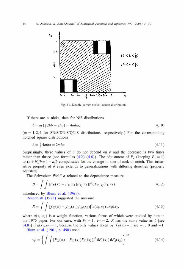
The changes in � are also associated with change in the relative positions to eachother of the black and blank areas. However, for SNiS or SNoS distributions theposition of the nick (or notch) has no e<ect on the value of � if it is moved laterally,as a whole, along the x2-axis within 06 x16 1. This is even true for DNiS or SNoSdistributions if the two nicks (or notches) are moved, independently of each other,along the relevant lines (x2 = 0; 1, respectively). Extreme cases are shown in Figs. 10and 11.

It is noteworthy, in all these cases, that, although symmetry of conditional distribu-tions is lost, the correlation is still zero, because of the neutral property of the nick(or notch), from which it is still true that

E[X1 |X2 = x2] = 12 for all x2 (0¡x2¡ 1):


Fig. 9. Extended nicked square distribution.

Fig. 10. Corner nicked square distribution.

There is an alternative measure of dependence

�=∫ 1

0

∫ 1

0|fX (x) − 1| dx1 dx2 (4.8)

(cited in Feuerverger, 1993) where fX (x) is the joint probability density function ofX1 and X2, that is much easier to evaluate than is �. In the present cases, it is simply

(P2 − 1) (area where density is P2(¿ 1)) + (area where density is zero): (4.9)


Fig. 11. Double corner nicked square distribution.

If there are m nicks, then for NiS distributions

�= m(ab2hb+ 2ha

)= 4mha; (4.10)

(m = 1; 2; 4 for SNiS/DNiS/QNiS distributions, respectively.) For the correspondingnotched square distributions

�= 12 4mha= 2mha: (4.11)

Surprisingly, these values of � do not depend on b and the decrease is two timesrather than thrice (see formulas (4.2)–(4.6)). The adjustment of P2 (keeping P1 = 1)to (a+ b)=b= 1 + a=b compensates for the change in size of nick or notch. This insen-sitive property of � even extends to generalizations with di<ering densities (properlyadjusted).

The Schweizer–Wol< � related to the dependence measure

B=∫ ∫

[FX (x) − FX1 (x1)FX2 (x2)]2 dFX1 ;X2 (x1; x2) (4.12)

introduced by Blum, et al. (1961).Rosenblatt (1975) suggested the measure

R=∫ ∫

[fX (x) − fX1 (x1)fX2 (x2)]2a(x1; x2) dx1dx2; (4.13)

where a(x1; x2) is a weight function, various forms of which were studied by him inhis 1975 paper. For our case, with P1 = 1; P2 = 2; R has the same value as � [see(4.8)] if a(x1; x2) = 1, because the only values taken by fX (x)− 1 are −1; 0 and +1.

Blum et al. (1961, p. 490) used

�F ={∫ ∫

[FX (x) − FX1 (x1)FX2 (x2)]2 dF1(x1) dF2(x2)}1=2

(4.14)


as a measure of departure from independence for comparing powers of di<erent testsof independence. Note also the neglected index for uniform distributions proposed byHoe<ding (1940) and de5ned in Section 1, which is closely related to �F , whosegeneral behavior ought to be similar to that of �.

We (Johnson and Kotz, 2000) have used an analog of �, de5ned by

�∗ = 12∫ 1

0

∫ 1

0|FX (x) − FX1 (x1)FX2 (x2)| dx2 dx1: (4.15)

The value of �∗ for SNiS is 12a2h(1 − h) [cf. � = 24a2h(1 − 12h)—see (A.15)]; the

value of �∗ for DNiS is 12a2h(1 − 2h) [cf. � = 24a2h—see (A.18)].In conclusion we would like to emphasize that the constructions and arguments

presented in this paper reveal subtleties and ambiguities involved in the seeminglystraightforward concept of dependence between two random variables. The multiplic-ity of possibilities has so far precluded obtaining a satisfactory universal measure ofdependence, even in these relatively simple situations.

5. Alternating double nicked square distribution

None of our nicked or notched square distributions have both marginal distributionsuniform. The design below (Fig. 12—alternating double nicked square distribution)does have both marginals uniform. Also X1 and X2 are uncorrelated because

E[X1 |X2 = x2] = 12 ∀x2 ∈ (0; 1):

Fig. 12. Alternating double nicked distribution.


However the conditional distribution of X1 given X2 =x2 is not uniform for 0¡x2¡h,or 1 − h¡x2¡ 1.

AlsoE[(X1 − 1

2 )r1 |X2 = x2]

6

(r1 + 1)−12−r1 for h¡x2¡ 1 − h;(r1 + 1)−12−r1 [1 + 2r1+1ar2{(2r2−1 − 1)} for 0¡x2¡h;

(r1 + 1)−12−r1{1 − 2r1+1ar2 (2r1−1 − 1)} for 1 − h¡x2¡ 1;

E[(X2 − 12 )r2 (X2 − 1

2 )r2 ] = 2−r1−r2 (r1 + 1)−1(r2 + 1)−1{(1 − 2h)r2 + 2hr2}:This value of � = 24a2h(1 − h).

Note that for the original SNiS distribution � = 24a2h(1 − 12h) and for the original

DNiS distribution � = 24a2h because the upper side adds 12a2h2. For the alternatingDNiS distribution, this is subtracted (without changing the sign of (FX (x) − x1x2) sowe get 24a2h(1 − 1

2h) − 12a2h2 = 24a2h(1 − h).Values of

∫ 10

∫ 10 {fX (x) − 1}2 dx1 dx2 and

∫ 10

∫ 10 |fX (x) − 1| dx1 dx2 are the

same as for original DNiS distributions— (because values of P1; P2, and P3 areunchanged).

Acknowledgements

The authors express their sincere thanks to Dr. C.B. Borkowf for his valuable com-ments and suggestions, and to Mrs. Teresita Abacan for her skillful typing and retypingof this paper.

Appendix A

In this section we outline derivation of expressions for joint product moments andfor the Schweizer–Wol< dependence measure �. We start with moments.

In all the cases described in Sections 2 and 3 the conditional distribution of X1 givenX2 = x2 is symmetric on [0; 1] for all x2 in [0; 1]. Hence

E[(X1 − 12 )r1 |X2 = x2] = 0 if r1 is odd: (A.1)

In the following calculations it will be supposed that r1 and r2 are even.For SNiS distributions

E[(X1 − 12 )r1 |X2 = x2] =

(r1 + 1)−12−r1 (h6 x26 1);

2(r1 + 1)−1[P1{2r1−1 − (a+ b)r1+1}+P2{(a+ b)r1+1 − ar1+1}]

= (r1 + 1)−12−r1 + 2(r1 + 1)−1b−1a(a+ b)

×{(a+ b)r1 − ar1} (06 x26 h):

(A.2)

(Since P1 = 1 and P2 = (a+ b)b−1.)


The marginal distribution of X2 is uniform [0; 1], so

�r1 ;r2 = E[(X1 − 12 )r1 (X2 − 1

2 )r2 ] = (r1 + 1)−12−r1 (r2 + 1)−12−r2

+ 2(r1 + 1)−1(r2 + 1)−1b−1a(a+ b){(a+ b)r1 − ar1}

×{(h− 12 )r2+1 − (− 1

2 )r2+1}: (A.3)

If a= b (with P1 = 1; P2 = 2),

�r1 ;r2 = E[(X1 − 12 )r1 (X2 − 1

2 )r2 ]

= (r1 + 1)−1(r2 + 1)−12−r1−r2 + D1(r1; r2; a); (A.4)

where D1(r1; r2; a) = 4(r1 + 1)−1(r2 + 1)−1(2r1 − 1)ar1+1{(h− 12 )r2+1 − (− 1

2 )r2+1}.For SNoS distributions with a= b (P1 = 1; P2 = 2)

E[(X1 − 12 )r1 |X2 = x2] =

(r1 + 1)−12−r1 (h6 x26 1);

(r1 + 1)−1{2−r1 + 4(2−r1 − 1)

×ar1+1(1 − x2h−1)r1+1}(06 x26 h):

(A.5)

�r1 ;r2 = E[(X1 − 12 )r1 (X2 − 1

2 )r2 ] = (r1 + 1)−1(r2 + 1)−12−r1−r2

+ 4(2r1 − 1)ar1+1r2∑j=0

(−1

2

)r2−j ( r2j

)hj+1B(j + 1; r1 + 2)

= (r1 + 1)−1(r2 + 1)−12−r1−r2 + D(r1; r2; a); say; (A.6)

where B(m; n) = (m− 1)!(n− 1)!=(m+ n− 1)! is the complete beta function. See Eqs.(11)–(14) in Section 3.

For double and quadruple distributions, we utilize the fact that each additional nickor notch contribute the same adjustment to the value of �r1 ;r2 as does the single nickor notch in the single distributions. Thus for DNiS distributions

�r1 ;r2 (double) = (r1 + 1)−1(r2 + 1)−12−r1−r2 + 2D1(r1; r2; a):

For quadruple distributions we must take into account that X1 and X2 (and so r1and r2) are interchanged for the two nicks or notches on the vertical lines (x2-axis andx2 = 1). Hence

�r1 ;r2 (quadruple) = (r1 + 1)−1(r2 + 1)−12−r1−r2

+2{D1(r1; r2; a) + D1(r2; r1; a)}: (A.7)


Explicit formulas are:DNiS

�r1 ;r2 = (r1 + 1)−1(r2 + 1)−1[2−r1−r2 + 8(2r1 − 1)ar1+1{(h− 12 )r2+1 − (− 1

2 )r2+1}]:(A.8)

QNiS

�r1 ;r2 = (r1 + 1)−1(r2 + 1)−1[2−r1−r2 + 8(2r1 − 1)ar1+1{(h− 12 )r2+1

−(− 12 )r2+1} + 8(2r2−1 − 1)ar2{(h− 1

2 )r1+1 − (− 12 )r1+1}]: (A.9)

DNoS

�r1 ;r2 = (r1 + 1)−1(r2 + 1)−1

2−r1−r2 + 8(2r1 − 1)ar1+1

×r2∑j=0

(−1)j(r2

j

)hj+1B(j + 1; r1 + 2)

: (A.10)

QNoS

�r1 ;r2 = (r1 + 1)−1(r2 + 1)−1

2−r1−r2 + 8

2∑i=1

(2ri − 1)ari+1

×ri∑j=0

(−1)j(ri

j

)hj+1B(j + 1; ri + 2)

: (A.11)

A.1. Calculation of the index �

We now proceed to calculation of the index

� = 12∫ 1

0

∫ 1

0|FX (x) − x1x2| dx1 dx2 = 12I; say:

This involves somewhat more complex considerations. In the present case, however,the piecewise uniform nature of the modi5ed distribution substantially facilitates thework. We will, for simplicity, restrict this analysis to the cases a= b; P1 = 1; P2 = 2.The possible values of the discrepancy from the uniform pdf are thus −1; 0, and 1Fig. 13 exhibit these regions for the case of SNiS distributions, with some examplesof the region (X16 x1) ∩ (X26 x2).

Apart from the “neutrality” of each complete nick or notch, we also use the symmetryof these modi5cations. The values of FX (x)− x1x2 in the right-hand half ( 1

2 6 x26 1)of the square (all nonpositive) are mirror images of those in the left-hand half (allnonnegative)—so that the values of |FX (x)−x1x2| are the same. We only need thereforeto evaluate just the values in the left-hand half and double them.


Fig. 13. Single nicked square distribution: deviation of density from uniformity. Values of fX (x) − 1.Examples of regions (X16 x1) ∩ (X26 x2) and bounded by region.

For SNiS distributions

FX (x) − x1x2 =

0 for 06 x16 12 − 2a; 06 x26 1;

(x1 − 12 + 2a)x2 for 1

2 − 2a6 x16 12 − a; 06 x26 h;

( 12 − x1)x2 for 1

2 − a6 x26 12 ; 06 x26 h;

(x1 − 12 + 2a)h for 1

2 − 2a6 x16 12 − a; h6 x26 1;

( 12 − x1)h for 1

2 − a6 x16 12 ; h6 x26 1:

Hence∫ 1

0

∫ 1=2

0|FX (x) − x1x2| dx1 dx2

=∫ h

0x2

∫ 1=2−a

1=2−2a(x1 − 1

2 + 2a) dx1 dx2

+∫ h

0x2

∫ 1=2

1=2−a( 1

2 − x1) dx1 dx2

+ h∫ 1

h

∫ 1=2−a

1=2−2a(x1 − 1

2 + 2a) dx1 dx2


+ h∫ 1

h

∫ 1=2

1=2−a( 1

2 − x1) dx1 dx2

= a2h(1 − 12h): (A.14)

Thus

I = 2a2h(1 − 12 h) and � = 24a2h(1 − 1

2 h): (A.15)

For DNiS distributions, we have to add the contribution from the nick on the linex2 = 1. The relevant additional values of FX (x) − x1x2 (all nonnegative) are:

FX (x) − x1x2 =

0 for 06 x16 12 − 2a

(06 x26 1);

(x1 − 12 + 2a)(h− 1 − x2) for 1

2 − 2a6 x16 12 − a;

1 − h6 x26 1;

( 12 − x1)(h− 1 − x2) for 1

2 − a6 x16 12 ;

1 − h6 x26 1;

0 for 12 − 2a6 x16 1

2 − a;06 x26 1 − h:

(A.16)

The additional contribution is∫ 1

0

∫ 1=2

0|FX (x) − x1x2| dx1 dx2

=∫ 1

1−h(x2 − 1 + h)

∫ 1=2−a

1=2−2a(x1 − 1

2 + 2a) dx1 dx2

+∫ 1

1−h(x2 − 1 + h)

∫ 1=2

1=2−a( 1

2 − x1) dx1 dx2

= 12a

2h2: (A.17)

Thus

I = 2a2h(1 − 12h) + a2h2 = 2a2h; which yields � = 24a2h: (A.18)

The situation is quite more involved for QNiS distributions. In this case the totalcontribution from the lateral nicks on the x2-axis and the line x2 = 1 are no longer allnonnegative on the left-hand half (06 x16 1

2 ) of the unit square and in fact whenthey are negative they can more than cancel out the total contributions from the nicksin the DNiS con5guration.


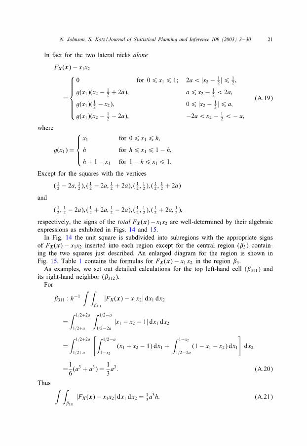
In fact for the two lateral nicks alone

FX (x) − x1x2

=

0 for 06 x16 1; 2a¡ |x2 − 12 |6 1

2 ;

g(x1)(x2 − 12 + 2a); a6 x2 − 1

2 ¡ 2a;

g(x1)( 12 − x2); 06 |x2 − 1

2 |6 a;

g(x1)(x2 − 12 − 2a); −2a¡x2 − 1

2 ¡− a;

(A.19)

where

g(x1) =

x1 for 06 x16 h;

h for h6 x16 1 − h;h+ 1 − x1 for 1 − h6 x16 1:

Except for the squares with the vertices

( 12 − 2a; 1

2 ); ( 12 − 2a; 1

2 + 2a); ( 12 ;

12 ); ( 1

2 ;12 + 2a)

and

( 12 ;

12 − 2a); ( 1

2 + 2a; 12 − 2a); ( 1

2 ;12 ); ( 1

2 + 2a; 12 );

respectively, the signs of the total FX (x)− x1x2 are well-determined by their algebraicexpressions as exhibited in Figs. 14 and 15.

In Fig. 14 the unit square is subdivided into subregions with the appropriate signsof FX (x) − x1x2 inserted into each region except for the central region ($3) contain-ing the two squares just described. An enlarged diagram for the region is shown inFig. 15. Table 1 contains the formulas for FX (x) − x1 x2 in the region $3.

As examples, we set out detailed calculations for the top left-hand cell ($311) andits right-hand neighbor ($312).

For

$311 : h−1∫ ∫

$311

|FX (x) − x1x2| dx1 dx2

=∫ 1=2+2a

1=2+a

∫ 1=2−a

1=2−2a|x1 − x2 − 1| dx1 dx2

=∫ 1=2+2a

1=2+a

[∫ 1=2−a

1−x2

(x1 + x2 − 1) dx1 +∫ 1−x2

1=2−2a(1 − x1 − x2) dx1

]dx2

=16

(a3 + a3) =13a3: (A.20)

Thus ∫ ∫$311

|FX (x) − x1x2| dx1 dx2 = 13a

3h: (A.21)


Fig. 14. Quadruple nicked square with regional subdivisions. �2 ≡ ⋃4j=1 �2j ; �3 ≡ ⋃4

j=1 �3j ; $1 ≡ ⋃4j=1 $1j ;

$2 ≡ ⋃4j=1 $2j ; $4 ≡ ⋃4

j=1 $4j ; $5 ≡ ⋃4j=1 $5j ; �2 ≡ ⋃4

j=1 �2j ; �3 ≡ ⋃4j=1 �3j or [�i ≡ ⋃4

j=1 �ij ;

�i ≡⋃4j=1 �ij(i = 2; 3) : $i ≡

⋃4j=1 $ij(i = 1; 2; 4; 5)].

Similarly for $312 we have:

h−1∫ ∫

$312

|FX (x) − x1x2| dx1 dx2

=∫ 1=2+2a

1=2+a

∫ 1=2

1=2−a|x1 − x2 − 2a| dx1 dx2

=∫ 1=2+2a

1=2+a

[∫ 1=2

x2−2a(x1 + 2a− x2) dx1 +

∫ x2−2a

1=2a(x2 − x1 − 2a) dx1

]dx2

=16

(a3 + a3) =13a3


Fig. 15. Map of region $3.

Table 1FX (x) − x1x2 for QNiS Distributions in the region $3

and ∫ ∫$312

|FX (x) − x1x2| dx1 dx2 = 13a

3h: (A.23)

In fact each of the eight cells in the upper left and lower right quadrants of $3

provide the same contribution ( 13a

3h) to I . Moreover the other eight cells (in the upper


Table 2Contributions

∫ 10

∫ 10 |FX (x) − x1x2| dx1 dx2; by regions

Regions Contribution (each region)

�1; �4; �1; �4 0$1; �2 4( 1

2a2)( 1

2 h2) = a2h2

�3; $2; $4; �3 4( 12a

2h)( 12 − 2a− h) = 2a2h( 1

2 − 2a− h)

�2; $5 4( 12a

2h)h + 4( 12a

2)( 12h

2) = 3a2h2

$311; $312; $321; $322

$333; $334; $343; $344

}13a

3

$313; $314; $323; $324

$331; $332; $341; $342

}a3

Total 2a2h2 + 8a2h( 12 − 2a− h) + 6a2h2 + 8( 1

3 + 1)a3

=4a2h(1 − 43a),

� = 48 a2h(1 − 43a): (A:25 bis).

right and lower left quadrants) each contribute a3h to I . Hence the total contributionto I from $3 is

8( 13 + 1)a3h= 32

3 a3h: (A.24)

Evaluation of contributions from the remaining regions using results already obtainedin this appendix is straightforward. The obtained values are exhibited in Table 2. Asindicated there, we obtain:

I = 4a2h(1 − 43a); thus � = 48a2h(1 − 4

3a): (A.25)

A.2. Evaluation of � for notched square distributions

For SNoS(and DNoS) distributions the same methods as those used for NickedSquare distributions can be used (see Fig. 16), but the following indirect methodmay be more convenient and could perhaps be utilized in other similarsituations.

For SNoS distributions (as is the case for SNiS as well) symmetry considerationsallow us to consider only the left-hand half of the square. The half notch shown inFig. 16 can be analyzed as if it is the value for a complete +1 half notch with baseof 2a minus twice a complete −1 half-notch with base of a (formally represented inFig. 17). Remember that outside the black area the di<erence in densities is zero inthe remainder of the left half of the unit square.


Fig. 16. Geometric representation of FX (x) − x1x2 for notched distributions.

Fig. 17. Representation of a half-notch.

Denote by %c the integral of |FX (x)− x1x2| over the interval 06 x16 12 due to the

triangular region as shown in Fig. 18. we then need to calculate

I =∫ 1

0

∫ 1

0|FX (x) − x1x2| dx1 dx2 = 2(%2a − 2%a): (A.26)

The equation of the sloping line in Fig. 18 is

x2 = (x1 − 12 + c)h=c; i:e: x1 = 1

2 − c + ch−1x2: (A.27)

For 06 x26 (x1 − 12 + c)h=c,

FX (x) − x1x2 = 12x2(x1 − 1

2 + c + x1 − 12 + c − ch−1x2)

= x2(x1 − 12 + c − 1

2 ch−1x2): (A.28.1)


Fig. 18. A generic region of integration of |FX (x) − x1x2| for single notched square distribution.

For (x1 − 12 + c) h=c6 x26 1,

FX (x) − x1x2 = 12 (x1 − 1

2 + c)2hc−1: (A.28.2)

In both (A.28.1) and (A.28.2), FX (x) − x1x2 is nonnegative. Of course for 06 x1

6 12 − c, and all x2, the di<erence FX (x) − x1x2 is zero.

Hence

%c =∫ 1

2

12−a

∫ (x1− 1

2 +c)h=c

0x2

(x1 − 1

2+ c − 1

2ch−1x2

)dx2

+∫ 1

(x1− 12 +c)h=c

12

(x1 − 1

2+ c)2

hc−1 dx2

]dx1: (A.29)

Substituting y = x1 − 12 + c we have

%c =∫ c

0

[∫ yh=c

0x2

(y − 1

2ch−1 x2

)dx2 +

∫ 1

yh=chc−1y2 dx2

]dy

= 18 (hc−1)c4 − 1

24(hc−1)2c4 + 1

6hc−1c3 − 1

2 (hc−1)2c4

= 16c

2h(1 − 14h): (A.29a)

Thus

I = 2(%2a − 2%a) = 23a

2h(1 − 14h) (A.30)

and

� = 12I = 8a2h(1 − 14h):

This is the value of � for SNoS distributions (with a= b). See Fig. 3.To evaluate I and � for DNoS distributions it is necessary to calculate the additional

contribution from the upper (on the line x2 = 1) triangle %′c, say, as schematically

indicated in Fig. 19.


Fig. 19. The upper generic triangle for double notched square distribution.

Now we have

%′c =

12hc−1

∫ h

0

∫ c

ch−1x′2

(y − ch−1x′2) dy dx′2 (x′2 = 1 − x2)

=12hc−1

∫ h

0

13c3(1 − h−1x′2)3 dx′2 = 1

24c2h2: (A.32)

Consequently

I = 2(%′2a − 2%′

a) = 16a

2h2: (A.33)

Fortunately, FX (x) − x1x2 is nonnegative over the range of integration for %′c so we

simply add this value of I to that for I in (A.30), giving

I = 23a

2h (A.34)

and

� = 8a2h

for DNoS distributions.

A.3. Calculations of � for QNoS distributions

Notes: (i) The diagram of cells in Fig. 15 also applies here. The contributionto FX (x) − x1x2 from the two pairs (lateral and double notched) are of the samesign in cells ($313; : : : ; $324) and of opposite signs in cells ($311; : : : ; $344) as inFig. 15.

(ii) We are assuming that∫ 1

0

∫ 10 FX (x) − x1x2| dx1 dx2 is the same for each of the

eight ‘same sign’ cells and for each of the eight ‘opposing sign’ cells.


(iii) Instead of following the calculation pattern in Table 2, we shall use the factthat if all cells were of the ‘same sign’ we would get twice the value for � as forDNoS distributions, i.e. 16a2h. However, we lose

8[(“same sign” cell contribution) − (“opposite sign” cell contribution)] from

∫ 1

0

∫ 1

0|FX (x) − x1x2| dx1 dx2:

Speci5cally, denote yj=xj− 12 . For the region $3 of Fig. 15, contribution to FX (x)−x1x2

from yj (j = 1; 2) are:For

a6yj6 2a; − 14ha (yj − 2a)2;

06yj6 a; − 14ha (yj − 2a)2 + 1

2ha (yj − a)2;

−a6yj6 0; 14ha (yj + 2a)2 − 1

2ha (yj + a)2;

−2a6yj6− a; − 14ha (yj + 2a)2:

For the ‘same sign’ cells, e.g. for cell $341 (−2a6y1; y26−a), we have contributionto∫ 1

0

∫ 10 |FX (x) − x1x2| dx1 dx2:

14ha

∫ −a

−2a

∫ −a

−2a(y1 + 2a)2 + (y2 + 2a)2 dy1 dy2

=2h4a

∫ −a

−2a

∫ −a

−2a(y1 + 2a)2 dy1 dy2 =

12ha

13

∫ −a

−2aa3 dy2 =

16ha3:

There are eight such cells—contribution to∫ 1

0

∫ 10 |FX (x)−x1x2| dx1 dx2 is 8× 1

6ha3=

(4=3)ha3.For “opposite signs” cells, e.g. in cell $311 (−2a6y16 − a; a6y26 2a);

(y1 + 2a)2 7 (y2 − 2a)2 according as −y1 ? y2.Hence the contribution to

∫ 10

∫ 10 |FX (x) − x1x2| dx1 dx2 is[

14ha

∫ −a

−2a

∫ 2a

−y1

[(y1 + 2a)2 − (y2 − 2a)2] dy2 dy1

−∫ −a

−2a

∫ −y1

a[(y2 − 2a)2 − (y1 + 2a)2] dy2 dy1

]

=2 × 14ha

∫ −a

−2a

∫ 2a

−y1

[(y1 + 2a)2 − (y2 − 2a)2] dy2 dy1

= 12 × h

a23

14a

4 = 112 ha

3:

There are 8 such cells and the contribution to I =∫ 1

0

∫ 10 |FX (x) − x1x2| dx1 dx2 is

thus (2=3)ha3.


Table 3Summary (a = b;P1 = 1; P2 = 2)

Distribution �

SNiS 24 a2h(1 − 12 h)

DNiS 24 a2hQNiS 48 a2h(1 − 4

3 a)

SNoS 8 a2h(1 − 14h)

DNoS 8 a2hQNoS 16 a2h (1 − 1

2a)

If we just add two (lateral and original DNoS) �’s, we get 16a2h. The loss fromopposing signs is

12( 43 − 2

3 )ha3 = 8ha3:

Thus � for QNoS distribution is

16 a2h− 8ha3 = 16 a2h(1 − 12a):

We note that (i) for:

Single distributions 0¡a¡ 14 ; 0¡h¡ 1; for

Double distributions 0¡a¡ 14 ; 0¡h¡ 1

2 and for

Quadruple distributions 0¡a; 2a+ h¡ 12 ; 06 h

(both for nicked and notched)

(ii) (a) max a2h= max a2 max h for single and double cases.Single: max a2 = ( 1

4 )2; max h= 1, implying max a2h= 116 .

Double: max a2 = ( 14 )2; max h= 1

2 , implying max a2h= 132 .

(b) Quadruple: max a2h= maxa a2( 12 − 2a) = ( 1

6 )2( 12 − 1

3 ) = 1216 .

(c) max a2h(1 − wh) = max a2max{h(1 − wh)} for single and double cases.Single: max a2h(1 − wh) = ( 1

4 )2(1 − w) = 116 (1 − w) (06w6 1

2 ).Double: max a2h(1 − wh) = ( 1

4 )2 12 (1 − 1

2w) = 132 (1 − 1

2w).

See Table 3.

References

Blum, J.R., Kiefer, J., Rosenblatt, M., 1961. Distribution free tests of independence based on the sampledistribution function. Ann. Math. Statist. 32, 485–498.

Borkowf, C.B., Gail, M.H., Carroll, R.J., Gill, R.D., 1997. Analyzing bivariate continuous data grouped intocategories de5ned by empirical quantiles of marginal distributions. Biometrics 53, 1054–1069.

Feuerverger, A., 1993. A consistent test for bivariate dependence. Internat. Statist. Rev. 61, 419–433.Hoe<ding, W., 1940. Masztabinvariante korrelationslehre. Schrift. Math. Inst. Angew. Math. Univ. Berlin

5 (3), 181–233.


Johnson, N.L., Kotz, S., 2000. On an L1-measure of dependence for modi5ed bivariate distributions. StatisticaLX (1), 3–16.

Johnson, N.L., Kotz, S., 1999. Non-smooth sailing. Triangular distribution revisited after 50 years. J. Roy.Statist. Soc. Ser. D 48, 179–187.

Rosenblatt, M., 1975. A quadratic measure of deviation of two-dimensional density estimates and a test ofindependence. Ann. Statist. 3, 1–14.

Schweizer, B., 1991. Thirty years of copulas. In: Dall’Aglio, G., Kotz, S., Salinetti, G. (Eds.), Proceedings,Symposium on Distributions with Given Marginals. Kluwer, Dordrecht, The Netherlands, pp. 13–50.

Schweizer, B., Wol<, E.F., 1981. On nonparametric measures of dependence for random variables. Ann.Statist. 9, 879–885.

Documents

Some novel models of distributions over the unit square