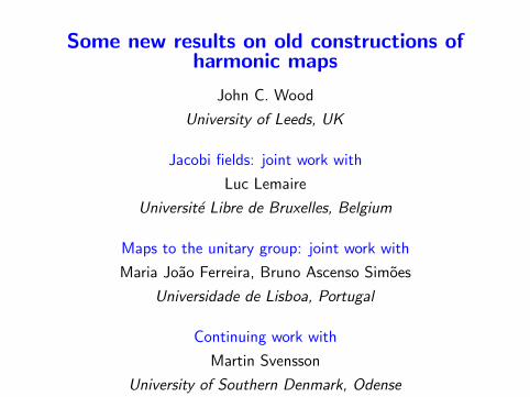
Some new results on old constructions ofharmonic maps

John C. Wood

University of Leeds, UK

Jacobi fields: joint work with

Luc Lemaire

Universite Libre de Bruxelles, Belgium

Maps to the unitary group: joint work with

Maria Joao Ferreira, Bruno Ascenso Simoes

Universidade de Lisboa, Portugal

Continuing work with

Martin Svensson

University of Southern Denmark, Odense

j.c.wood@leeds.ac.uk

http://www.maths.leeds.ac.uk/pure/staff/wood/wood.html

Harmonic maps

Let ϕ : (M, g)→ (N, h) be a smooth map between compactsmooth Riemannian manifolds. The energy or Dirichlet integralof ϕ is

E (ϕ) =

∫M

e(ϕ)ωg =

∫M

12 |dϕ|

2 ωg

where ωg = volume measure and, for any x ∈ M,

|dϕx |2 = Hilbert–Schmidt norm2 of dϕx = g ijhαβ ϕαi ϕ

βj .

The map ϕ is called harmonic if the first variation of E forvariations ϕt of the map ϕ vanishes at ϕ, i.e., d

dt E (ϕt)∣∣t=0

= 0.We compute

ddt

E (ϕt)∣∣t=0

= −∫

M

⟨τ(ϕ), v

⟩ωg

where v = ∂ϕt/∂t|t=0 is the variation vector field of (ϕt), andτ(ϕ) = div dϕ is the tension field of ϕ given as follows:

Tension field of a map ϕ

τ(ϕ) = div dϕ = Trace∇dϕ =m∑

i=1

∇dϕ(ei , ei )

=m∑

i=1

∇ϕei

(dϕ(ei )

)− dϕ(∇M

eiei )

;

τ(ϕ)γ = g ij

(∂2ϕγ

∂x i∂x j− Γk

ij

∂ϕγ

∂xk+ Lγαβ

∂ϕα

∂x i

∂ϕβ

∂x j

)= ∆Mϕγ + g(grad ϕα, grad ϕβ) Lγαβ .

∆M = Laplacian on functions f : M → R:

∆Mf = div grad f = div df = −d∗df = Trace∇df

=m∑

i=1

ei

(ei (f )

)−(∇M

eiei

)f

=1√|g |

∂

∂x i

(√|g | g ij ∂f

∂x j

).

Examples of harmonic maps

ϕ : M → N is harmonic ⇐⇒τ(ϕ) ≡ Trace∇dϕ = 0 (Harmonic equation)

1. ϕ : Rm ⊇ U → Rn is harmonic iff ∆ϕ = 0(∆ = usual Laplacian on Rm).

2. ϕ : (M, g)→ Rn is harmonic iff ∆Mϕ = 0(∆M = Laplace–Beltrami operator on (M, g) ).

3. ϕ : R ⊇ U → N or S1 → N is harmonic iff it defines a geodesicparametrized linearly.

4. Holomorphic maps between Kahler manifolds are harmonic; infact they give absolute minima of the energy functional.

5. Harmonic morphisms, i.e., maps which preserve Laplace’sequation, are harmonic maps.

Weakly conformal maps

A smooth map ϕ : (M, g)→ (N, h) is called weakly conformal(with conformality factor λ) if ϕ∗h = λ2g ; explicitly, for all p ∈ M,

h(dϕp(X ),dϕp(Y )

)= λ(p)2 g(X ,Y ) (X ,Y ∈ TpM) ;

equivalently,dϕ∗p dϕp = λ(p)2 IdTpM .

In local coordinates, this reads

hαβϕαi ϕ

βj = λ2gij .

A. Sanini: A non-constant map ϕ is extremal with respect tovariations of the metric iff dim M = 2 and ϕ is weakly conformal.Proof. The Euler–Lagrange operator for such variations is thestress-energy tensor S(ϕ) = e(ϕ)g − ϕ∗h. If this is zero, takingthe trace shows that dim M = 2, then comparing with the above,shows that ϕ is weakly conformal (with λ2 = e(ϕ) ).

Conformal invariance in 2 dimensions

Harmonic maps from surfaces are conformally invariant in thesense that the composition ϕ ψ of a harmonic map ϕ : M2 → Nfrom a surface with a weakly conformal map ψ : M ′2 → M2 ofsurfaces is harmonic.In fact, if (x , y) are isothermal coordinates on M2, the harmonicequation reads

∇ϕ∂/∂x

(∂ϕ∂x

)+∇ϕ∂/∂y

(∂ϕ∂y

)= 0 .

If we write z = x + iy , this reads

∇ϕ∂/∂z

(∂ϕ∂z

)= 0 , equivalently, ∇ϕ∂/∂z

(∂ϕ∂z

)= 0 .

Hence the concept of harmonic map from a Riemann surface iswell defined. Further, ϕ : M2 → N is harmonic if and only if∂ϕ/∂z is holomorphic with respect to the Koszul–Malgrangeholomorphic structure on ϕ−1TN → M.

Harmonic maps and minimal surfaces

Let ϕ : M2 → N be a weakly conformal map with conformalityfactor λ. Then, away from branch points, the mean curvature is2λ2 times the tension field, hence:

A weakly conformal map is harmonic if and only if it is minimalaway from branch points.

Such a map is called a minimal branched immersion.

[W. and others] Any harmonic map from the 2-sphere is weaklyconformal and so is a minimal branched immersion.Proof. The (2, 0)-part of the stress energy tensor

S(ϕ)2,0 ≡⟨∂ϕ∂z

,∂ϕ

∂z

⟩is a holomorphic section of T ∗1,0S2. Such a section must vanishsince this bundle has negative degree.

Harmonic maps from surfaces to CPn

Holomorphic maps M2 → CPn are harmonic, as areantiholomorphic maps.When n = 1 and M2 = S2, this accounts for all harmonic maps.

When n > 1, we can find harmonic maps which are not±-holomorphic, as follows:

Given a harmonic non-±-holomorphic map ϕ = [Φ] : M2 → CPn ithas two Gauss transforms, a ∂′- and a ∂′′-transform:

G ′(ϕ) =[π⊥ϕ

∂Φ

∂z

], G ′′(ϕ) =

[π⊥ϕ

∂Φ

∂z

].

These can be extended over points where the derivatives are zero,and are both harmonic. If ϕ is holomorphic (resp.antiholomorphic), only G ′(ϕ) (resp. G ′′(ϕ)) is defined.

[J. Eells–W., 1983] All harmonic maps from S2 → CPn areobtained from holomorphic maps by applying the ∂′-Gausstransform up to n times.

An example

Let f (z) = [F (z)] = [1, z3, z2]. This defines a (smooth)holomorphic map from S2 to CP2 (note that f (∞) = [0, 1, 0]).

We calculate its Gauss transform G ′(f ) at each z as theorthogonal complement of f (z) in the first osculating spacef(1)(z) spanned by F (z) and F ′(z).

Now F ′(z) = (0, 3z2, 2z) so that (F ∧ F ′)(z) = (−z4,−2z , 3z2);note that this is zero at z = 0 because f has a branch point there.However, it equals z ψ(z) where ψ(z) = (1, z3, z2) ∧ (0, 3z , 2) isnon-zero for all z . So f(1)(z) is the plane spanned by (1, z3, z2)and (0, 3z , 2) and G ′(f )(z) is the orthogonal complement of theline f (z) in that plane. Hence G ′(f ) is smooth at the branchpoint z = 0. Calculating at z =∞ by replacing z by w = 1/z , wesee that G ′(f ) is smooth there too.

We thus obtain a harmonic map G ′(f ) : S2 → CP2 which isnot holomorphic or antiholomorphic.

Skip to Explicit talk

Smoothness of the Gauss transform

For any harmonic map ϕ : M2 → CPn, its Gauss transformG (1)(ϕ) is a smooth map, but is the map G (1) : ϕ 7→ G (1)(ϕ)smooth, or even continuous? In general, no:Example Let ft : S2 → CP2 be ft(z) = [Ft(z)], where

Ft(z) = (1, tz + z3, z2) (z ∈ C, t ∈ R)

(so that ft(∞) = [0, 1, 0]). Note that ft is a smooth family of fullholomorphic maps. Then G ′(ft)(0) = [0, 1, 0] ∀t 6= 0 butG ′(f0)(0) = [0, 0, 1].

Details We compute F ′t(z) = (0, t + 3z2, 2z) and so

Ft ∧ F ′t(z) = (tz2 − z4,−2z , t + 3z2) .

If t 6= 0, at z = 0 this equals (0, 0, t) = t(1, 0, 0) ∧ (0, 1, 0).

Details of the last example, continued

It follows that the first associated curve has the value

ft(1)(0) = span(1, 0, 0), (0, 1, 0)and G ′(ft)(0) = [0, 1, 0] .

However, if t = 0, then

Ft ∧ F ′t(z) = (−z4,−2z , 3z2) = zψ(z)

where ψ(z) = (−z3,−2, 3z). In particularψ(0) = (0,−2, 0) = 2(1, 0, 0) ∧ (0, 0, 1) so that

f0(1)(0) = span(1, 0, 0), (0, 0, 1)and G ′(f0)(0) = [0, 0, 1] .

This shows that ft(1) and G ′(ft) do not vary continuously with t.The reason for this is that ft is unramified when t 6= 0 but ramifiedwith ramification index 1 at z = 0 when t = 0, and that in thepresence of ramification, ft(1) involves division of polynomials bytheir common factor, a discontinuous process when the degree ofthe factor changes.

Recovering smoothness

• Holk(S2,CP2) = (connected) component of the space ofholomorphic maps of degree k ;• Harmd ,E (S2,CP2) = the component of the space of harmonicmaps of degree d and energy 4πE .

[Lemaire–W., 1996] The Gauss transformHolk(S2,CP2)→ Harm(S2,CP2) restricts to a diffeomorphism:

Holfullk,r (S2,CP2)→ Harmfull

d ,E (S2,CP2) .

where r = ramification index, d = k − r − 2, E = 3k − r − 2.

Example Let ft : S2 → CP2 be defined by

Ft(z) =(z4 + 1, (1− 3t2)z3 + (−3t + t3)z , 2tz2 + (1− t2)

)(z ∈ C, t ∈ R) (so that ft(∞) = [1, 0, 0]). When t 6= 0, ft isramified at z = ±

√t with index 1; when t = 0, these ramification

points coalesce into a ramification point at z = 0 of index 2.

Then G ′(ft) is a smooth family of harmonic maps.

Details of the smooth example

Identifying S2 with C ∪ 0 by stereographic projection, letft : S2 → CP2 be defined by

Ft(z) =(z4 + 1, (1− 3t2)z3 + (−3t + t3)z , 2tz2 + (1− t2)

)(z ∈ C, t ∈ R) (so that ft(∞) = [1, 0, 0]).Identifying Λ2C3 with C3 we have (Ft ∧ F ′t)(z) = (z2 − t)ψ(z)where

ψ(z) =((−2t + 6t3)z2 + (−3 + t2)(1− t2),

4z(tz2 + 1), (−1 + 3t2)z4 + 8tz2 + 3− t2)

which shows that, if t 6= 0, ft is ramified at z = ±√

t with index 1,but if t = 0, these ramification points coalesce into a ramificationpoint at z = 0 of index 2. Further ft(1)(z) = [ψ(z)]. We see fromthis that ft ∈ Holfull

4,2(CP2) for all t and that ft(1) and so G ′(ft)vary smoothly with t, even though each root does not.

Second Variation

Let ϕt,s be a 2-parameter variation of ϕ ;

write v =∂ϕt,s

∂t

∣∣∣(0,0)

and w =∂ϕt,s

∂s

∣∣∣(0,0)

. The Hessian of ϕ is:

Hϕ(v ,w) =∂2E

∂t∂s(ϕt,s)

∣∣∣(0,0)

=

∫M〈Jϕv ,w〉ωg

whereJϕv = ∆ϕv − Trace RN(dϕ, v)dϕ

is called the Jacobi operator along ϕ, and∆ϕv = −Trace∇2 is the Laplacian on ϕ−1TN.

Observation If ϕt is a one-parameter family of maps with ϕ0 = ϕand ∂ϕt

∂t

∣∣t=0

= v , then

Jϕ(v) = − ∂

∂tτ(ϕt)

∣∣∣t=0

.

Corollary If ϕt is a one-parameter family of harmonic maps withϕ0 = ϕ, then v = ∂ϕt

∂t

∣∣t=0

is a Jacobi field along ϕ, i.e., Jϕ(v) = 0.

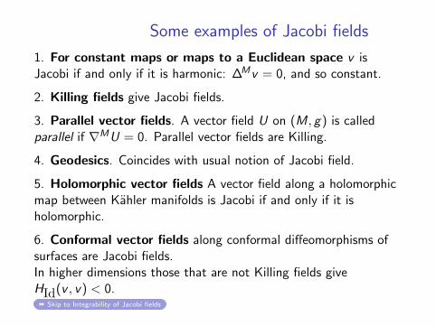
Some examples of Jacobi fields

1. For constant maps or maps to a Euclidean space v isJacobi if and only if it is harmonic: ∆Mv = 0, and so constant.

2. Killing fields give Jacobi fields.

3. Parallel vector fields. A vector field U on (M, g) is calledparallel if ∇MU = 0. Parallel vector fields are Killing.

4. Geodesics. Coincides with usual notion of Jacobi field.

5. Holomorphic vector fields A vector field along a holomorphicmap between Kahler manifolds is Jacobi if and only if it isholomorphic.

6. Conformal vector fields along conformal diffeomorphisms ofsurfaces are Jacobi fields.In higher dimensions those that are not Killing fields giveHId(v , v) < 0.

Skip to Integrability of Jacobi fields

Some examples of Jacobi fields

7. For the identity map Jacobi operator is

JId = ∆H − 2 RicM = 0. (1)

[K. Yano and T. Nagano] who called Jacobi fields geodesic vectorfields.

8. When (M, g) is Einstein with RicM = c Id (c constant),formula (1) reads

JId = ∆H − 2c Id .

[R.T. Smith] The nullity of identity map = the multiplicity of 2cas an eigenvalue of ∆M plus the dimension of the space of Killingfields.

9. Jacobi fields on spheres. nullity(IdSm) = m(m + 1)/2 ifm 6= 2, and 6 if m = 2.

10. Harmonic variations [G. Toth]. ϕt = exp(tv) is harmonic forall t ∈ R =⇒ v is Jacobi.

Some general results on Jacobi fields

An interpretation [M.-J. Ferreira]

A vector field v along a smooth map ϕ : M → N is harmonic as amap M → (TN, complete lift metric) if and only if ϕ is harmonicand v is a Jacobi field along it.

The negative curvature case

Suppose that Riem (N) ≤ 0. Then any Jacobi field v along aharmonic map M → N is parallel along the map.

For the identity map N → N, v is Jacobi iff it is Killing.

If, further, Ric(N) < 0 at some point, any Jacobi field along theidentity map is zero.

Integrability of Jacobi fields

Definition A Jacobi field v along a harmonic map ϕ is said to beintegrable if there is a one-parameter family (ϕt) of harmonic

maps with ϕ0 = ϕ and∂ϕt

∂t

∣∣∣t=0

= v .

Big Question: When are all Jacobi fields integrable?

Why is this important?

1. [D. Adams and L. Simon] Let (M, g) and (N, h) bereal-analytic Riemannian manifolds. If all Jacobi fields alongharmonic maps from M to N are integrable, then Harm(M,N) is areal-analytic manifold with tangent space the space of Jacobifields.

2. [Adams–Simon, R. Gulliver and B. White] If all Jacobifields are integrable, we get information on the singular set of aharmonic map and rate of blowing up near the singular set.

Cases where all Jacobi fields are integrable

1. Jacobi fields along constant maps and maps into Euclideanspaces;

2. [W. Ziller, 1977] M = S1 and N = a globally symmetricspace;

3. [Besse, 1978] M = S1 and N = a manifold all of whosegeodesics are closed (i.e., periodic) and of the same length;

4. [T. Sunada, 1979] M arbitrary, N = a locally symmetric spacewith Riem (N) ≤ 0;

5. [Gulliver and White, 1989] M = N = S2 = CP1;

6. [Lemaire and W., 2002] M = S2 and N = CP2;

Cases where not all Jacobi fields areintegrable

1. [Algrem and others, 1970s] M = S1 and N = a surface ofrevolution with R = 0 along a geodesic of revolution and R < 0elsewhere;

2. [Mukai, 1997] M = S1 × S1 and N = S3;

3. [Lemaire and W., 2008] M = S2, N = Sn (n = 3, 4);

4. [In progress] M = S2, N = CPn (n ≥ 3), N = Sn (n ≥ 5).Skip to Jacobi fields for S2 → S4

The space of harmonic maps for negativecurvature

1. Riem N < 0 [Hartman, 1967]

Harmf (M,N) = point, unless f is constant or has image a circle.In this case, all Jacobi fields are zero.

2. Riem N ≤ 0 [Schoen–Yau, 1979]

If M, N are Cω, then Harmf (M,N) is parametrized by a compactmanifold N0. Precisely, there is a mapF : M × N0 → N such that

Harmf (M,N) = F |M×t : t ∈ N0 ,

and, for any p ∈ M, F |p×N0is an isometric immersion onto a

totally geodesic submanifold.However, in this case, it is not necessarily true that all Jacobi fieldsare integrable.

Harmonic maps from S2 to S4

1. [Calabi, 1967] Each harmonic map ϕ : S2 → S4 is + or − theprojection of a horizontal holomorphic maps f : S2 → CP3 intothe twistor space CP3 of S4; the ±-sign is called the spin of ϕ.

If f has degree d , then ϕ has energy 4πd . The components ofHarm(S2,S4) are thus parametrized by d ∈ 1, 2, . . ..

2. (Full and non-full maps) Either ϕ is a ±-holomorphic mapS2 → S2 followed by a totally geodesic inclusion of S2 in S4 or ϕis (linearly) full.

Harmonic maps from S2 to S4, contd

3. [Verdier, 1985] The harmonic maps of energy 4πd form aconnected complex algebraic variety Harmd(S2,S4) of puredimension 2d + 4. This has three irreducible components if d ≥ 3.

a. One component is the subset HarmNFd (S2,S4) of non-full

harmonic maps of energy 4πd ; this is a (non-empty) closedcomplex manifold of dimension 2d + 4.

b. The subset of full harmonic mapsHarmLF

d (S2,S4) is empty for d = 1, 2, and is a non-empty with twoconnected components Harm+

d (S2, S4) and Harm−d (S2,S4) ford ≥ 3; these components are smooth manifolds when d = 3, 4, 5[Bolton and Woodward, 2004].

For any d ≥ 3, their closures are the other two irreduciblecomponents of Harmd(S2,S4).

Jacobi fields along harmonic maps fromS2 to S4

Theorem [Lemaire and W., 2006]. (i) There is a one-to-onecorrespondence between the Jacobi fields along a full harmonicmap ϕ : S2 → S4 (of positive spin) and the infinitesimal horizontalholomorphic deformations of its twistor lift f : S2 → CP3.

(ii) Let Cd = set of limit points of HarmLFd (S2,S4) in

HarmNFd (S2, S4) (‘collapse points’). Cd is non-empty for d ≥ 3

[Ejiri–Kotani, Guest–Ohnita, Montiel–Ros].

(iii) For ϕ ∈ HarmNFd (S2,S4), all Jacobi fields along ϕ are

integrable if and only if ϕ 6∈ Cd .

(iv) Let ϕ : S2 → S2 ⊂ S4 be in Cd . Consider ϕ as inHarmd(S2,S3). Then there are non-integrable Jacobi fieldsalong it, although Harmd(S2,S3) is a manifold.

Example of a collapse

For t ∈ R, define ft : S2 → CP3 by

ft = [z ,−3tz2, z3 + 1, t] .

For t 6= 0 this is a full horizontal holomorphic map of degree 3.

As t → 0, it approaches the non-full horizontal holomorphic mapf0 = [z , 0, z3 + 1, 0].

Setting ϕt = π ft gives a family of full harmonic mapsϕt : S2 → S4 which ‘collapse’ to a non-full harmonic mapϕ0 : S2 → S2, z 7→ (z3 + 1)/z.

Thus ϕ0 ∈ C3, showing it is non-empty.Skip to Maps to the unitary group

Harm(S2, Sn)

[Calabi 1967] HarmLFd (S2, S2m) is non-empty if and only if

d ≥ 12 m(m + 1).

[Barbosa 1975] For d = 12 m(m + 1),

HarmLFd (S2,S2m) = O(2m + 1,C).

[Kotani 1992] Harmd(S2, Sn) is path connected.

[Furuta–Guest–Kotani–Ohnita 1992] calculateπ1 Harmd(S2,Sn).

[Bolton and Woodward 2001] For d = 12 m(m + 1) + 1,

HarmLFd (S2,S2m) = CP2 \ Q ×O(2m + 1,C).

[Bolton and Woodward, conjecture, proved by L. Fernandez,2003, 2005] dimC Harmd(S2,S2m) = 2d + m2.

Harm(S2, CPn)

[Guest–Ohnita 1993 + Crawford 1997]The connected components of Harm(S2,CPn) areHarmk,E (S2,CPn).

[Segal, Crawford 1993] The inclusions

HolLFk (S2,CPn) → Holk(S2,CPn) → C 0(S2,CPn)

are homotopy equivalences, the first to dimension 2(k − n), thesecond to dimension k(2n − 1).

[Crawford 1993] determines the homology of HolLFk (S2,CP2).

Harmonic maps from unitons

The Gauss transform is an example of Uhlenbeck’s operation ofadding a uniton (also called flag transform) which transformsharmonic maps M2 → U(n) into others, as follows:Any smooth map ϕ defines a connection Aϕ = 1

2ϕ−1dϕ, and thus

a covariant derivative Dϕ = d + Aϕ, on the trivial bundleCn = M2 × Cn ; writing Aϕ = Aϕz dz + Aϕz dz , since Aϕz represents∂ϕ/∂z , Harmonicity of ϕ is equivalent to holomorphicity of Aϕz .

A uniton for ϕ is a subbundle α of the trivial bundle which isholomorphic, i.e, closed under Dϕ

z , and closed under Aϕz .Then [K. Uhlenbeck, 1989]:

(i) If ϕ : M2 → U(n) is harmonic and α is a uniton for ϕ,then ϕ = ϕ(πα − π⊥α ) is harmonic.

(ii) Any harmonic map ϕ : S2 → U(n) can written as a finiteproduct of unitons:

ϕ = const. (πα1 − π⊥α1) · · · (παr − π⊥αr

) . (2)

Return to Unique Factorization Theorem Skip to General Construction

Building all harmonic maps

To build all harmonic maps we add unitons α1, α2, . . . starting withthe constant map, giving a sequence of harmonic mapsϕ0 = const., ϕ1 = ϕ0(πα1 − π⊥α1

),ϕ2 = ϕ1(πα2 − π⊥α2

) = ϕ0(πα1 − π⊥α1)(πα2 − π⊥α2

), . . ..To do this, we must know the possible unitons at each stage.For this, we must find a meromorphic basis for the trivial bundleCn with respect to Dϕi

z for each i ; in general, this involves solving∂-problems.

[M.J. Ferreira, B. Simoes, W., preprint, 2008]Every harmonic map can be built by adding unitons which aregiven in terms of projections along previous unitons ofmeromorphic functions, without solving ∂-problems.

This gives a completely explicit algebraic parametrization of allharmonic maps S2 → U(n) by meromorphic functions.

The general construction

TheoremAll non-constant harmonic maps from S2 → U(n) are given as a

product (2) in the following way for some r ∈ 0, 1, . . . , n :

Choose an r × n array of meromorphic functions Hi ,j : S2 → Cn,(i = 0, . . . , r − 1, j = 1, . . . , n); these could be zero.

For i = 0, 1, . . . , r − 1, let αi+1 be the sum of subbundles α(k)i+1

(k = 0, . . . , i) with α(k)i+1 spanned by

i∑s=k

C is H

(k)s−k,j (j = 1, . . . , n) .

Here C is =

∑1≤i1<···<is≤i π

⊥is· · ·π⊥i1 , and the superscript (k)

denotes the k ’th derivative.

The first few formulae

(i) α1 is the subbundle α1 = α(0)1 = spanH0,j .

(ii) α2 is the sum of subbundles α2 = α(0)2 + α

(1)2 where

α(0)2 = spanH0,j + π⊥α1

H1,j ,

α(1)2 = spanπ⊥α1

H(1)0,j .

(iii) α3 is the sum α3 = α(0)3 + α

(1)3 + α

(2)3 where

α(0)3 = spanH0,j + (π⊥α1

+ π⊥α2)H1,j + π⊥α2

π⊥α1H2,j ,

α(1)3 = span(π⊥α1

+ π⊥α2)H

(1)0,j + π⊥α2

π⊥α1H

(1)1,j ,

α(2)3 = spanπ⊥α2

π⊥α1H

(2)0,j .

Return to Unitons to meromorphic data Skip to Grassmannian model

Examples

A smooth (resp. holomorphic) map α : M2 → Gk(Cn) is the samething as a smooth (resp. holomorphic) subbundle α of Cn.The Grassmannians Gk(Cn) are included in U(n) via the Cartanembbedding B 7→ πB − π⊥B . This is a totally geodesic isometrywhich identifies the disjoint union G∗(Cn) of these Grassmannianswith the subset B ∈ U(n) : B = B∗ = B ∈ U(n) : B2 = I.

A harmonic map into G∗(Cn) is thus the same as a harmonic mapinto U(n) with image in this subset.

1. If the data (Hi ,j) has only one non-zero entry H0,1, then

α1 = spanH0,1 and α2 = spanH0,1+ spanπ⊥α1(H

(1)0,1 ). The

formula gives ϕ2 = the ∂′-Gauss transform G ′(α1) of α1.

2. More generally, if each column of (Hi ,j) has only one non-zeroentry, then the unitons are nested: αi ⊂ αi+1, and ϕ is anisotropic map into a Grassmannian.

Unique factorization–1

The data gives a sequence of unitons satisfying the followingcovering condition due to G. Segal: πi (αi+1) = αi for all i .

TheoremGiven a harmonic map ϕ : M2 → U(n) there is a unique factorization

(2) into proper unitons satisfying the covering condition with α1

full.

Proof. We recall that any harmonic map ϕ gives rise to a loop ofsmooth maps Φλ called an extended solution for ϕ as follows.With Aϕ = 1

2ϕ−1dϕ, write Aϕ = Aϕz dz + Aϕz dz and set

Aϕλ = 12 (1− λ−1)Aϕz dz + 1

2 (1− λ)Aϕz dz . Then ϕ harmonic impliesdAϕλ + [Aϕλ ,A

ϕλ ] = 0, the integrability condition for solving

12 Φ−1

λ dΦλ = Aϕλ .

We let Φλ be any smooth solution. Note that Φ1 is constant, wetake it to be I , and Φ−1 equals ϕ up to left equivalence, i.e., up toleft multiplication by an element of U(n).

Unique factorization–2

A harmonic map ϕ : M2 → U(n) is said to be of finite unitonnumber if if can be written as the product of unitons:

ϕ = ϕ0(πα1 − π⊥α1) · · · (παr − π⊥αr

).

The minimal number of unitons required is called the unitonnumber of ϕ. An extended solution for ϕ is:

Φ = (πα1 + λπ⊥α1) · · · (παr + λπ⊥αr

).

A harmonic map ϕ is of finite uniton number if and only if it has apolynomial extended solution:

Φ = T Φ0 + λT Φ

1 + · · ·+ λr T Φr .

This is unique if we insist that the Im T Φ0 be a full subbundle. The

degree of Φ is then the uniton number of ϕ.

Unique factorization–3

Given a harmonic map ϕ of uniton number r , we find a unitonfactorization into proper covering unitons inductively as follows.

(i) Set Φr = Φ, the unique extended solution of ϕ with Im T Φ0 full.

(ii) Suppose we have defined an extended solution Φi of degree i(for some harmonic map ϕi ) with non-zero constant term, setα⊥i = Im (T Φi

i )∗, and Φi−1 = Φi (π⊥αi

+ λπαi ). This is a polynomialof degree i − 1 with non-zero constant term.

(iii) The process terminates after exactly r steps with Φ0 = Igiving a factorization into proper unitons satisfying the coveringcondition. The fullness of Im T Φ

0 translates into fullness of α1.

(iv) The Φi are extended solutions for the product of the first iunitons: Φ = (πα1 + λπ⊥α1

) · · · (παi + λπ⊥αi).

(v) Clearly Im (T Φii )∗

= Im(π⊥αi · · · π⊥α1

). The coveringcondition implies that this is equal to α⊥i , establishing uniqueness.

Unitons to meromorphic data–1

TheoremLet α1, α2, . . . be a sequence of unitons satisfying the coveringcondition. Then they are given by the formulae above for somemeromorphic data Hi ,j .

Proof.1. We start with a constant map ϕ0, so that the first uniton α1 isa holomorphic subbundle of Cn, and so is given by the span ofsome meromorphic functions K0 = H0.This gives us a harmonic map ϕ1 = ϕ0(πα1 − π⊥α1

).

2. The meromorphic sections K0 of α1 remain meromorphic for(Cn,Dϕ1

z ) — a special property of this first step.

Meromorphic sections of α⊥1 are all of the form π⊥α1H1 where H1 is

a meromorphic vector. We conclude that the most generalmeromorphic section of (Cn,Dϕ1

z ) is of the form K1 = H0 + π⊥α1H1

so that α2 must be spanned by sections of this form.

Unitons to meromorphic data–2

3. We set ϕ2 = ϕ1(πα2 − π⊥α2) .

The sections of the form K1 give a basis for α2, and aremeromorphic with respect to Dϕ1

z but they are not, in general,meromorphic with respect to Dϕ2

z . However sections of the form

H0 + (π⊥α1+ π⊥α2

)H1

are meromorphic with respect to Dϕiz and project under πα2 to K1.

To complete a basis we prove that for any meromorphic H2,π⊥α2

π⊥α1(H2) is a meromorphic section of α⊥2 ; by the covering

condition, this gives all such, so all meromorphic sections of(Cn,Dϕ1

z ) are of the form

H0 + (π⊥α1+ π⊥α2

)H1 + π⊥α2π⊥α1

(H2) .

Hence α3 must be spanned by sections of this type.

4. We set ϕ3 = ϕ2(πα3 − π⊥α3), . . .

Grassmannian model interpretation–1

Let ΩalgU(n) denote the algebraic loop group consisting of allmaps γ : S1 → U(n) with γ(1) = I of the form

γ(λ) =∑t

i=s Tiλi

for some integers s, t and some Ti ∈ gl(n,C).

Let H denote the Hilbert space L2(S1,Cn) and let H+ denote theclosed subspace of elements of the form

∑k≥0 λ

kak whereak ∈ Cn.

The loop group ΩalgU(n) acts on H and the map γ 7→ γ(H+)identifies ΩalgU(n) with the algebraic Grassmannian, consisting ofall subspaces W of H such that λW ⊂W andλsH+ ⊂W ⊂ λtH+ for some s, t.

Grassmannian model interpretation–2

A polynomial extended solution can be thought of as a smoothmap Φ : M2 → ΩalgU(n).Setting W = Φ(H+) defines a map W from M2 to the algebraicGrassmannian.If Φ has degree r , the subspace W satisfies λrH+ ⊂W ⊂ H+,and so can be considered to be in the quotient space H+/λ

rH+.We thus obtain a map W : M2 → G∗(H+/λ

rH+) into theGrassmannian of the finite-dimensional vector space H+/λ

rH+ .Harmonic maps ϕ : M2 → U(n) of uniton number at most rcorrespond to holomorphic maps W : M2 → H+/λ

rH+∼= Crn, or

equivalently, holomorphic subbundles W of the trivial bundleM2 ×H+/λ

rH+∼= Crn satisfying

λW (1) ⊂W . (3)

Here, W (1) denotes the subbundle spanned by (local) sections ofW and their first derivatives (with respect to any complexcoordinate on M2).

Grassmannian model interpretation–3

Holomorphic subbundles W of M2 ×H+/λrH+ satisfying (3) are

given [M. Guest] by taking an arbitrary holomorphic mapX : M2 → G∗(H+/λ

rH+) ∼= G∗(Crn), equivalently, holomorphicsubbundle X of Crn, and setting W equal to the coset

W = X + λX (1) + λ2X (2) + · · ·+ λr−1X (r−1) + λrH+ . (4)

TheoremLet ϕ be given by an array (Hi ,j). Set

Li ,j =∑i

k=0

( ik

)Hk,j (5)

and let X be the subbundle spanned by∑r−1

i=0 λiLi ,j . Then W is

the Grassmannian model of ϕ.

Harmonic maps into a Grassmannian–1

Uhlenbeck proved that Φλ is a type one extended solution of aharmonic map ϕ : M2 → G∗(Cn) if and only if

Φλ = QΦ−λΦ −1−1 Q (6)

for some Q ∈ U(n) with Q2 = I , equivalently, Q = πC − π⊥C forsome C ∈ G∗(Cn). Further, in this case, QΦ−1 is a harmonic mapinto a Grassmannian.

Hence

LemmaLet Φ be the type one extended solution of a harmonic map offinite uniton number, say r , and let W = ΦH+ ∈ H+/λ

rH+ bethe corresponding Grassmannian model. Then Φ is the extendedsolution of a harmonic map into a Grassmannian if and only ifthere exists Q ∈ U(n) with Q2 = I such that

W λ = QW−λ (λ ∈ C) . (7)

Harmonic maps into a Grassmannian–2

DefinitionSay that a polynomial L ∈ H+/λ

rH+ is Q-adapted if itscoefficients have image alternately in C and C⊥, i.e.,L(λ) =

∑r−1i=0 Liλ

i and either(+) Li has image in C for i even, and in C⊥ for i odd, or(−) Li has image in C⊥ for i even, and in C for i odd;equivalently, L lies in either the (+1)- or the (−1)-eigenspace ofthe involution L(λ) 7→ QL(−λ) on H+/λ

rH+ .

Remark. When Q = I , a polynomial is Q-adapted if and only if itis even or odd, i.e, has coefficients of all odd or all even powers ofλ equal to zero.

Corollary

Φ is the extended solution of a harmonic map into a Grassmannianif and only if W has a spanning set consisting of Q-adaptedpolynomials, or, equivalently, W is given by (4) for some X whichhas a spanning set consisting of Q-adapted polynomials.

Ha maps into a Grassmannian–Example 1

Let r = 3, Q = I .

Let L0,1 and L2,1 be arbitrary meromorphic vectors, and let X bespanned by the even polynomial L0,1 + λ2L2,1. Then W is spanned

by this and by the odd polynomial λL(1)0,1; both polynomials are

Q-invariant with Q = I .

Via (5), X corresponds to a single column (H0,1, 0,H2,1)T of datawhere H0,1 = L0,1 and H2,1 = L2,1 + L0,1. Taking H0,1 = L0,1 andH2,1 = L2,1 gives the same unitons and so the same harmonic map.

α1 = spanH0,1, α2 = (α1)(1) = spanH0,1,H(1)0,1 and

α3 = spanH0,1 + π⊥2 H2,1, π⊥1 H

(1)0,1 , π

⊥2 H

(2)0,1.

From (28), ϕ : M2 → G2(C4) is given by

ϕ = spanH0,1 + π⊥2 H2,1, π⊥2 H

(2)0,1 .

Assuming that α1 is full, ϕ has uniton number three.

Ha maps into a Grassmannian–Example 2

r = 2, Q 6= I . Let Q = πC − π⊥C where C is a proper subspace ofCn. Let Li ,j (i = 0, 1, j = 1, 2) be meromorphic vectors where L0,1

and L1,2 have values in C but L0,2 and L1,1 have values in C⊥.

Let X be spanned by L0,j + λL1,j (j = 1, 2). Then W is spanned

by these and by λL(1)0,j (j = 1, 2), and all four polynomials are

Q-adapted. Note that (5) gives H0,j = L0,j and H1,j = L1,j − L0,j ,but we obtain the same unitons, and so the same harmonic map,from the data Hi ,j = Li ,j .

Then α1 = spanL0,1 = H0,1, L0,2 = H0,2; we can choose thisdata such that α1 is full — it suffices to have no linear relationbetween their components.

α2 = spanπ1L0,j + π⊥1 L1,j = H0,j + π⊥1 H1,j , π⊥1 L

(1)0,j =

π⊥1 H(1)0,j (j = 1, 2).

So ϕ = Q(π1 − π⊥1 )(π2 − π⊥2 ) : M2 → G∗(Cn) is a harmonic mapof uniton number two into a Grassmannian.

Isotropic maps

Suppose that X is spanned by monomials of the form λkLk ;equivalently, the data (Hi ,j) is in the ‘diagonal’ form

H0,1 · · · H0,d1 0 · · · 0 0 · · · 0 0 · · ·0 · · · 0 H1,d1+1 · · · H1,d2 0 · · · 0 0 · · ·0 · · · 0 0 · · · 0 H2,d2+1 · · · H2,d3 0 · · ·...

......

......

......

......

.... . .

then the unitons αi are nested, i.e., αi ⊂ αi+1. The projections in (28)

are unnecessary and αi+1 = spanH(`)i−`,k : 1 ≤ k ≤ d

(0)i+1, 0 ≤ ` ≤ i.

The harmonic map ϕ = (π1 − π⊥1 ) · · · (πr − π⊥r ) has image in aGrassmannian and is given by the formula

ϕ(⊥) =

[(r−1)/2]∑k=0

α⊥r−1−2k ∩ αr−2k = α⊥r−1 ∩ αr ⊕ α⊥r−3 ∩ αr−2 ⊕ · · · ,

where we set α0 equal to the zero subbundle. We thus obtain a harmonicmap into a Grassmannian which is isotropic in the sense that it isinvariant under the natural S1 action of C.-L. Terng.

Explicit formulae for any factorization

Recall that polynomial extended solution Φ : M2 → ΩalgU(n) ofdegree r defines a holomorphic subbundle W = Φ(H+) of thetrivial bundle H+/λ

rH+∼= M2 × Cn, which satisfies W (1) ⊂W .

G. Segal showed that the sequence of harmonic mapsΦ0 = I ,Φ1, . . . ,Φr = Φ coming from a factorization into unitons

Φi = (πα1 + λπ⊥α1) · · · (παi + λπ⊥αi

) (i = 0, 1, · · · , r)

corresponds, via W i = ΦiH+, to a filtration

W = W r ⊂W r−1 ⊂ · · · ⊂W 1 ⊂W 0 = H+,

with λW i ⊂W i+1.

Theorem (M. Svensson and JCW, 2009)

For any factorization/filtration, we have the following explicitformula for the unitons:

αi =i−1∑s=0

S i−1s PsW i . (8)

Further, the projection converts a holomorphic basis of W i into abasis holomorphic with respect to the harmonic map ϕi−1.

In fact, the formula (8) is equivalent to

αi = P0Φi−1W i

and we can show that P0Φi−1 converts the operators ∂z and λ∂z

on Wi−1 into Dz and −Aϕi−1z on Cn, respectively.

Example

Set W i = W + λiH+. Then we obtain the factorization satisfyingSegal’s covering condition

πi (αi+1) = αi for all i .

Note that the rank of the unitons increases with i . The W i in (8)can be replaced by W and we obtain the ‘Lisbon’ formulae for theunitons.

Example

Set W i = (λi−r W ) ∩H+ + λiH+. Then we obtain Uhlenbeck’sfactorization which satisfies the ‘dual’ covering condition

πi+1(αi ) = αi+1 for all i .

Note that the rank of the unitons decreases with i . This time, wecannot replace the W i in (8) by W . We obtain the formulae of B.Dai and C.-L. Terng.

Harmonic maps into 0(n) and Sp(n)

Given any λ-closed subspace Wr with λrH+ ⊂Wr ⊂ H+ andr ≥ 2, consider the subspace

Wr−2 = λ−1Wr ∩H+ + λr−2H+

This can be obtained from Wr by first doing a ‘Segal’-step:

Wr−1 = Wr + λr−1H+

and then an ‘Uhlenbeck’-step:

Wr−2 = λ−1Wr−1 ∩H+ + λr−2H+

or vice versa.

Say Wr is real if r = 2s and W⊥

= λ1−r Wr ; equivalentlyλ−sW = ΦH+ for some Φ ∈ ΩalgO(n).

LemmaIf Wr is real so is Wr−2.

Apply this to the (type one) extended solution Φ of a harmonicmap of finite uniton number into O(n), starting with Wr = ΦH+.

This gives a factorization of harmonic maps of finite unitonnumber from a surface to O(n), with explicit formulae provided by(8) given a meromorphic basis of W .

Similarly, for Sp(n), replacing ‘real’ by ‘symplectic’ and complexconjugation by J, obtaining an explicit version of R. Pacheco’sfactorization (2006).

j.c.wood@leeds.ac.uk

http://www.maths.leeds.ac.uk/pure/staff/wood/wood.html

Bibliography for Jacobi fields

L. Lemaire and JCW, On the space of harmonic 2-spheres inCP2, Internat. J. Math. 7 (1996) 211–225.

L. Lemaire and JCW, Jacobi fields along harmonic 2-spheres inCP2 are integrable, J. London Math. Soc. 66 (2002), 468–486.

JCW, Jacobi fields along harmonic maps, DifferentialGeometry and Integrable Systems, Contemp. Math., 308(2002), 329–340, American Math. Soc.

L. Lemaire and JCW, Jacobi fields along harmonic 2-spheres inS3 and S4 are not all integrable, Tohoku Math. J. (to appear).

Bibliography for maps into U(n), p.1

F. E. Burstall and M. A. Guest, Harmonic two-spheres incompact symmetric spaces, revisited, Math. Ann. 309 (1997)541–572.

B. Dai and C.-L. Terng, Backlund transformations, Wardsolitons, and unitons, J. Differential Geom. 75 (2007) 57–108.

M. J. Ferreira, B. A. Simoes and JCW, All harmonic 2-spheresin the unitary group, completely explicitly (preprint,arXiv:0811.1125, 2008).

M. A. Guest, An update on harmonic maps of finite unitonnumber, via the zero curvature equation, Integrable systems,topology, and physics (Tokyo, 2000), 85–113, Contemp. Math.309, Amer. Math. Soc., Providence, RI, 2002.

Bibliography for maps into U(n), p.2

Q. He and Y. B. Shen, Explicit construction for harmonicsurfaces in U(N) via adding unitons, Chinese Ann. Math. Ser.B 25 (2004) 119–128.

R. Pacheco, Harmonic two-spheres in the symplectic groupSp(n), Internat. J. Math. 17 (2006), 295–311.

G. Segal, Loop groups and harmonic maps, Advances inhomotopy theory (Cortona, 1988), 153–164, London Math.Soc. Lecture Note Ser., 139, Cambridge Univ. Press,Cambridge, 1989.

M. Svensson and JCW, Filtrations, factorizations and explicitformulae for harmonic maps (in preparation).

K. Uhlenbeck, Harmonic maps into Lie groups: classicalsolutions of the chiral model, J. Differential Geom. 30 (1989)1–50.