Some Methodological Flaws in Mainstream Economic Theories and the Implications of Constant Marginal Cost Curve

Xiaolin Zhong

Candidate of MA in Political Science, University of Lethbridge

1/31/2015

Introduction

Mainstream economic theories contain numerous methodological

flaws. By mainstream economic theories, I mean those professed in most

common economics text books, for such book is supposed to reflect

mainstream thoughts. Here are some examples of such flaws.

First, in economics text books, GDP is defined as the quantitative

measurement of final products. Final products mean the goods and services

that are solely for consumption, not those which serve as inputs, with or

without further process, of other goods or services. As a production factor,

capital goods are also excluded. The purpose of such definition is to avoid

double counting. For instance, the value of a car includes that of all of its

parts. If the values of the car and its parts are both counted, production

would clearly be unduly inflated. By definition, therefore, final products are

consisted of consumer goods only. In the same text books, however, the

formula calculating GDP equates it with the sum of consumptions,

government expenditures and investments. Such a formula seems to

constitute a direct contradiction to the definition of GDP. For the sake of

consistency, the formula should include only consumption. Such account

makes some sense, for consumption means goods and services not only

produced, but also consumed. Given the huge shrink of the book value of

wealth, let alone the write-off of billions of goods and services annually, it

seems to mean little to take into account the goods and services that are

merely produced, but have yet to be consumed.

1

This self-contradiction could have been regarded as a stupid, but

harmless joke, had GDP been something that no one pays attention to.

Unfortunately, this is not the case. GDP has long been postulated by elite

economists and many politicians all over the world, with unsurpassed efforts,

as one of the most desirable things, not only economically, but also

politically. It has been used as a major justification to expand unlimitedly the

political and spending power of the state. Chinese Communist Party, for

instance, declares that GDP is the single greatest source of happiness, and

its ability to build GDP in the highest speed in the world ultimately justifies

its one-party regime. As such, the GDP thing is not a matter that can be

taken lightly.

Second, the notion of increasing marginal cost is the underlying

assumption of the positively sloped supply curve of a commodity in a partial

market developed by Alfred Marshall. It is said that the producer would only

respond to price rise with more supply, for the increase in production causes

marginal cost to rise. The increased marginal cost has to be compensated by

the increase in price (1920, 346). This curve renders it possible for Marshal

to produce a general equilibrium between demand and supply by having it

intercept the negatively sloped demand curve. This theory has been taught

at almost all economics courses and seldom challenged. Its underlying

assumption, the notion of increasing marginal cost, however, appears

problematic.

2

The notion of increasing marginal cost seems to have its root in the

notion of diminishing return to scale. As Walter Nicholson points out, the

latter was first brought forward by David Richardo (1997, 8). Based on his

observation that more and more poorly fertilized land was utilized, Richrdo

predicted the price of grain would rise, for it requires more labour to produce

an extra bushel of grain. He considered such phenomenon quite common

and thus developed the generalized notion that labour and other costs would

tend to rise with the expansion of production of a particular good. This is

essentially an equivalent of the notion of increasing marginal cost, although

the marginalism had yet to emerge. It follows that prices would constantly

rise. Tomas Malthus made a much direr prediction: Human beings would be

destroyed, for population grows at a far more rapid pace than does food.

These predictions, however, have never substantiated, as Nicholson

indicates. Not only have relative prices remained largely stable, but, thanks

to the improvement of productive technologies, prices tend to fall and the

level of material conditions of human life has been raised tremendously

(1997, 9). Ricardo and Malthus have never been regarded as unwise, and

rightly so. Our knowledge is limited by what we can see. At the time of

Ricardo and Malthus, the production technology was such that the marginal

productivity of one factor, despite diminishing, is still greater than zero. With

such production technology, who would disagree with the notions of

diminishing return to scale and increasing marginal cost? However, with the

failure of these predictions, the modern production technology as such that

3

the marginal productivity of one factor falls to zero, and the continuous

improvement in production technologies and falling relative prices, it does

not appear wise to stick with these notions. There should have accumulated

a thick layer of literature that challenges them and Marshall’s equilibrium

itself. Such, however, does not seem to be the case. It appears few have paid

attention to this issue. Nicholson, for instance, has no problem with these

notions, despite his clear awareness and disclosure of the failure of the

predictions.

Third, in labs, it is impossible to have only one variable keep changing

while holding all others constant in experiments that test cause-effect

relations. In mainstream economic theories, however, any variable can be

arbitrarily singled out to change alone. For instance, price can be assumed to

change without the simultaneous change of any other variables, such as

income. This problem is also seen the Marshall’s equilibrium analysis.

Fourth, the Philips curve suggests that there is a trade- off between

inflation and employment. There has never been, however, any convincing

analysis of the inherent connection between the two. This theory is thus

basically built solely on statistics data. We have seen how absurd such

“theories” can be. The statistician, for instance, has found the positive

connection between peace and the number of McDonalds. Another example

is the positive connection between drinking capacity and the likelihood to be

hired. Not only is Philip’s Curve unsound a theory, but it has long been

4

proven phony by the stagflation during the 70’. It is still, however, upheld by

mainstream economists and serves as a theoretical basis for Fed’s monetary

policies.

With these flaws, mainstream economics is far from an established

science. A surgery on it is needed. This paper serves as a tiny part of the

surgery. Clearly, all the flaws indicated above have significant implications. A

paper such as this, however, cannot analyze all of them. I pick up the notion

of increasing marginal cost for two reasons. The first one is that its problems

have yet to draw sufficient attention. Since it is the underlying assumption of

Marshall’s theory of equilibrium and this theory is foundational to economics

as a whole, such lack of attention seems inadequate. The second is that the

analysis of this issue inevitably touches upon other flaws.

I will argue that, under modern production technology, marginal cost is

constant. The combination of constant marginal cost and fixed cost entails

declining average cost. Since price and average cost both drop as supply

expands, it is profitable for the firm to drop price in exchange for higher

volume of sales, until the point just before the two drops become equalized.

This indicates a negatively sloped supply curve. Demand and supply

intercept one another at the point where price equals average cost. This is

the real equilibrium point. The equilibrium in short run, however, is actually a

direction that economic activities tend to approach, but can never be

reached. In long run, it itself moves towards more supply and lower prices.

5

This is how economic grows. Money printing distorts prices and therefore is

counterproductive. Government spending squeezes the firm’s productive

indirect inputs and therefore is counterproductive as well. It also squeezes

the consumption of valuable goods and services by the consumer and

therefore is harmful to consumption.

The Major Difficulties Facing Marshall’s Theory of Equilibrium

As indicated earlier, Marshall’s theory of the equilibrium between

demand and supply of a commodity is built on an unsustainable underlying

assumption. It seems inevitable for a theory as such to be confronted with

serious difficulties. Discussed in the following several paragraphs are three

major ones: It does not sit well with the rule of profit maximization and

contradicts a common business practice; it does not explain why and how

prices change; and, it does not explain economic growth.

Note that at the point of profit maximization, marginal revenue equals

marginal cost. The equilibrium, however, seems to suggest that demand and

supply intercept one another at the point where price equals marginal cost.

Price is certainly not marginal revenue. This point therefore is not necessary

the one at which profit is maximized. This invites the question that, without

the firm’s maximum profit, how the equilibrium is to be reached. Note also

that, in the rule of profit maximization, marginal revenue is a downwardly

sloped curve. This is consistent with the downwardly sloped demand curve

which reflects the concept of diminishing marginal utility. Such curve

6

indicates that it is profitable for the firm to respond to falling price with more

supply. This does not seem to contradict reality. It is seen every day that

more we purchase, the lower the prices. The supplier seems to literally drop

prices in exchange for higher volume of sales. Such practice sharply

contradicts the notion that the producer only responds to rising prices with

more production.

It can be seen that this equilibrium theory implies that the producer is

merely a passive responder to the change in price. It can be by no means a

contributor. The consumer cannot be the game changer, either. Let us not

forget the caveats Marshall himself brings about for this theory: The income

of consumers remains unchanged, so are the prices of substitutes and

competitive products. Without the change of these variables, there does not

seem to be anyway for price to change. Without the change in price, neither

the producer nor the consumer will make any move. Thus, everything is

permanently frozen once the equilibrium is reached. This certainly makes no

sense whatever and contradicts the notion Marshal holds himself that it is

the interactions between the supplier and consumer that determine price

level. One may argue that, according to the notion of complete competition,

the producer is indeed incapable of changing price, so such incapability

should not constitute any problem. Not only that. Since it remains

unchanged, price becomes an equivalent of marginal revenue. The

incompatibility between the equilibrium point and the point of maximum

profit is thus removed. The problem with this line of argument is that the

7

notion of complete competition is confined with the same difficulty. It leaves

the cause for price change unexplained. To overcome this obstacle, some

proponents of the notion have gone so far as to invent an imaginary

“arbitrator” who calls the shots, literally turning economics as a science into

superstition.

There might be an opposition to this critique out of a methodological

argument. It would take the following path. In cause – effect relations

analysis, it is necessary to keep other variables fixed to determine the

effects of the change of one variable. It is legitimate therefore to analyze the

effects of the change in price without taking into account the change in other

variables, such as income. Such argument seems ignorant of a basic

scientific truth. Any change in any variable must be caused by the change of

at least one other variable. There is no way whatever to have a variable

move and keep its root cause constant simultaneously. Unless the change in

the root cause makes no difference, it cannot be ignored. Apparently, the

entire dynamic of the equilibrium analysis will be changed if income cannot

be kept fixed. This is why Marshall tries to exclude it from the picture in the

first place. This underpins the change in income must be taken into account.

Marshall is certainly right to realize that income must be frozen for him to be

able to proceed with his analysis. He forgot to ask himself, however, how

price can be changed in the first place.

8

It is interesting to note that the economist seems to have turned a

major disadvantage for the establishment of theories in social sciences into

advantage. The disadvantage refers to the fact that many of social scientific

hypotheses can hardly be tested in laboratory, because of either the

impossibility to setup laboratory environment or ethical concerns. The

physicist seems largely immune to such problem. He does have to, however,

worry about how to separate variables. On the contrary, the economist

worries about no such things. He simply takes it for granted that, not only

hypotheses in economic theories can be tested, but each variable can be

separated from one another with no restrains whatever. He thus not only has

removed the difficulty in hypothesis testing, but also accomplished with his

pen what is impossible for the physicist to accomplish in laboratory. Such

approach is certainly convenient. However, it does not appear convincing at

all.

Now let us try to figure out what happens if the caveats Marshall

himself imposed are relaxed. As indicated earlier, the entire dynamic of the

equilibrium analysis will be changed if income enters the picture.

Nevertheless the increase of income does cause prise to rise according to

the analysis. This is illustrated by an outward shift of the demand curve. A

closer scrutiny reveals, however, such shift appears highly unlikely. This is

because that, by definition, income comes from production. Thus, before

income can be increased, an expansion in production has to occur first.

Remember that the producer is merely a passive responder to the change in

9

price. Without increase in price in the first place, therefore, there is no way

for the producer to expand production. We are thus trapped in an

unbreakable circle. One may point out that production expansion does not

have to be originated from the producer whose product has already reached

the equilibrium point. It is perfectly conceivable that such expansion comes

out of the initiatives of those producers whose product have yet to reach

equilibrium. This point makes sense to a degree. It will run out of, however,

ammunition as the general equilibrium – a simultaneous equilibrium for all

products in all markets – is reached. It seems more troublesome to try to

melt the frozen income. Now, the entire economy is permanently frozen. It

can hardly be seen how the economic grows. What about the change in the

prices of substitute and competitive products? Such change does bring

about the price change of the particular commodity in question. It is,

however, by no means a way out of the circle. Such change is brought about

by the change of consumer preference. Its result is thus basically of zero-

sum.

With these difficulties, Marshall’s equilibrium seems to be a house built

on sand. A house as such is not repairable. It has to be torn down and a new

one built on solid foundation is needed.

The Downwardly Sloped Average Cost Curve as Supply Curve

As we have seen, the notion of increasing marginal cost is grounded on

the observations on outdated economic reality. As the foundation of

10

Marshall’s equilibrium, it renders the equilibrium confronted with numerous

sever difficulties that can hardly be overcome. To see if equilibrium between

supply and demand indeed exists, we need first to find out that, in modern

production, how marginal cost changes as output does. It turns out that

marginal cost changes proportionally with the change in output.

Marginal cost is the cost resulted from the usage of direct inputs. The

slope of the curve of this function is determined by production functions that

reflect different technologies. To find this slope in modern production, we

need to pin down modern production technology that dictates modern

production function. As Nicholson indicates, Leontief production function

reflects the production technology vastly employed in the real-world

production. Exceptions are rare (155, 1997). It is therefore the best

candidate for our analysis, for conclusions based on such technology can

largely be generalized. The production technology reflected by Leontief

production function is such that the ratios among all direct inputs, such as

machine and direct labour hours and raw materials, are fixed. The marginal

productivity of any single input is zero without the proportional increase of

all other inputs. This clearly exhibits a constant marginal cost, for each unit

of output requires precisely the same combination of direct inputs. It can be

seen that total marginal cost changes proportionally with the change of

output.

11

Note that Leontief production function does not include indirect inputs.

This is not only reasonable, but inevitable, for no numerical relationship can

be established between output and indirect inputs. When it comes to cost,

however, it would be a grave mistake to ignore indirect inputs, for the costs

associated with them constitute a great portion of total cost. The total cost

function therefore must include the costs associated with indirect inputs.

Since such costs do not change proportionally with the change of output,

they are treated as fixed cost. The total cost function associated with

Leontief production functions is thus

TC=f (Q )=MCQ+F (1)

Where TC represents total cost, MC marginal cost, Q output and F fixed cost.

Such total cost function is the only one taught by all cost accounting text

books with no exception. This is another indication of the dominance of the

production technology reflected by Leontief production function.

Fixed cost is largely associated with administrative activities, such as

management, research and development, finance and accounting,

marketing, etc. Such activities are necessary regardless of production

technologies. There is little doubt that they have been carrying more and

more weight in modern production. It would not seem exaggerating to assert

that indirect inputs are far more important than direct inputs in modern

production. It follows that fixed cost is much more significant than variable,

or marginal, cost. Fixed cost, however, has been constantly overlooked by

12

the economist in cost analysis. This is perhaps because there is nothing

marginal about it. This is true in absolute terms. In relative terms, however,

it is another matter. Precisely because fixed cost hardly changes as output

does, average fixed cost changes as output changes. It declines as output

increases. This is significant. For it gives us a diminishing average cost curve

which indicates a negatively sloped supply curve.

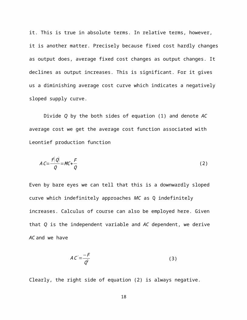
Divide Q by the both sides of equation (1) and denote AC average cost

we get the average cost function associated with Leontief production

function

AC=f (Q )Q

=MC+ FQ

(2)

Even by bare eyes we can tell that this is a downwardly sloped curve which

indefinitely approaches MC as Q indefinitely increases. Calculus of course

can also be employed here. Given that Q is the independent variable and AC

dependent, we derive AC and we have

AC'=−FQ2

(3)

Clearly, the right side of equation (2) is always negative.

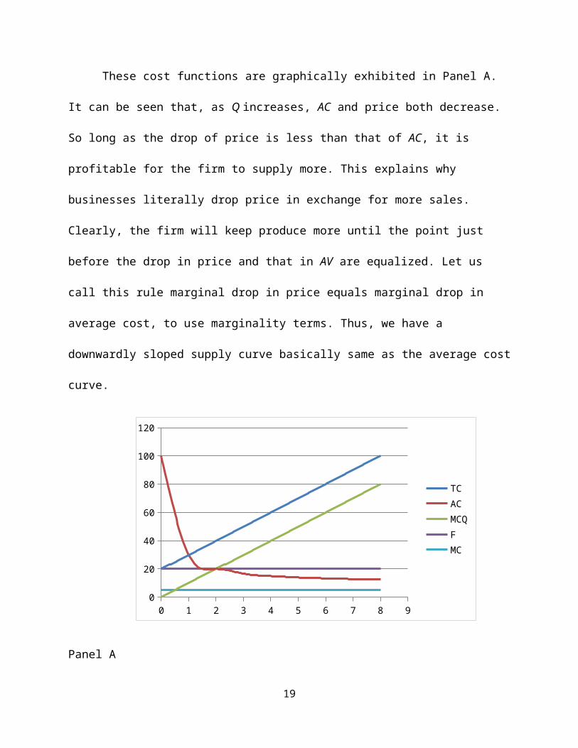
These cost functions are graphically exhibited in Panel A. It can be

seen that, as Q increases, AC and price both decrease. So long as the drop of

price is less than that of AC, it is profitable for the firm to supply more. This

explains why businesses literally drop price in exchange for more sales.

13

Clearly, the firm will keep produce more until the point just before the drop

in price and that in AV are equalized. Let us call this rule marginal drop in

price equals marginal drop in average cost, to use marginality terms. Thus,

we have a downwardly sloped supply curve basically same as the average

cost curve.

0 1 2 3 4 5 6 7 8 90

20

40

60

80

100

120

TCACMCQFMC

Panel A

Profit Maximization, Price, the Equilibrium, the Law of Increasing

Return to Scale and Economic Growth

As suggested earlier, if the equilibrium indeed exists, it must satisfy

the requirement of the rule of profit maximization. By intuition, we can see

from the earlier discussion that profit maximization is reached at the point

where marginal drop of price equals that of average cost. This does not,

however, tells us very much about levels of price and output at that point.

We still need the existing rule that marginal cost equals marginal revenue. 14

Calculus cannot help here, for it has never been established that the total

revenue function, a component of the profit function, is derivable (who says

that economists are mathematicians?). We thus have to find another way to

prove the rule. Fortunately, we do not have to start from scrap, for the cost

accountant has offered one long time ago. We just need to borrow it from

him.

It all starts with the idea of break-even point at which the firm neither

suffers loss nor attains profit. The cost accountant finds that, before this

point, the entire difference between price and marginal cost contributes to

the recovery of fixed cost. The total contribution required to recover entire

fixed cost is (denoting P price)

(P−MC )Q=F (4)

Break-even is reached with this total contribution, for entire fixe cost is

recovered. The break-even point is therefore

Q= F(P−MC )

(5)

Beyond this point, all difference between price and marginal cost contributes

solely to profit. It can be seen that any orders are acceptable as long as

marginal revenue exceeds marginal cost until the two are equalized. As

such, the existing rule of profit maximization holds.

15

What is the price level at this point? We find this by taking a look at the

total revenue. It is the sum of total cost and maximized profit, written

PQ=MCQ+F +¿ π ' (6)

Here π ' is the maximized profit.

Since F and π ' are both constants, we can mathematically combine

them into one. Considering maximized profit is an obligation of the firm, it

can be deemed a component of fixed cost. Thus we rewrite equation (6)

PQ=MCQ+F (7)

This says that total revenue equals total cost. Dividing Q by both sides of

equation (7) we get

P = FQ + MC (8)

Clearly, the right side of equation (8) is average cost. So we have

P=AC (9)

Note that Austrian School has said all along that value is determined

by utility. Utility, however, is different for different persons. It appears

somehow difficult to decide where price level can be settled. Here we see

that it is settled at average cost.

16

S1

p’ S2

p’’ D

q’ q’’

Q

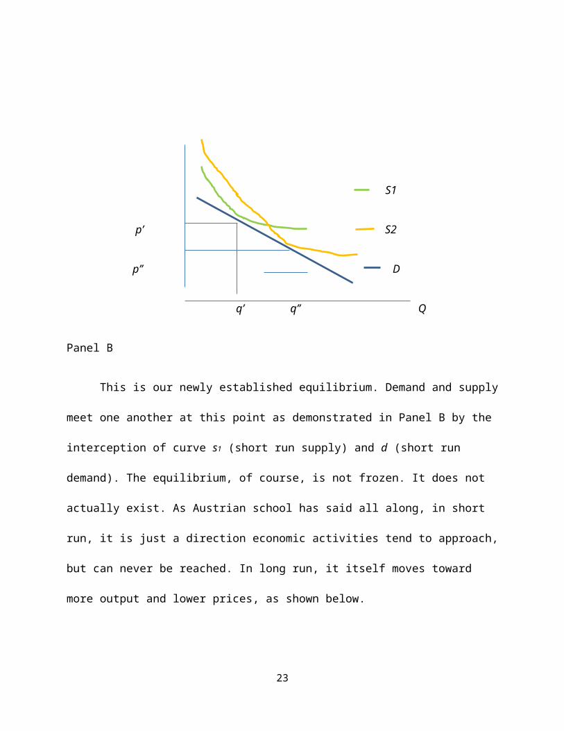
Panel B

This is our newly established equilibrium. Demand and supply meet

one another at this point as demonstrated in Panel B by the interception of

curve s1 (short run supply) and d (short run demand). The equilibrium, of

course, is not frozen. It does not actually exist. As Austrian school has said all

along, in short run, it is just a direction economic activities tend to approach,

but can never be reached. In long run, it itself moves toward more output

and lower prices, as shown below.

As discussed earlier, the notion of increasing marginal cost has much

to do with the notion of diminishing return to scale. Note that at the time of

Richardo, the dominant production technology was such that the marginal

productivity of one factor is declining. Note also that indirect inputs, while

existing, carried far less weight in production than they do today. Under such

conditions, diminishing return to scale was the law at that time. This law,

however, has become a thing of the past. Under the dominant production

17

technology today, marginal direct inputs remain constant. Total direct inputs

change proportionally with the change in output. This clearly exhibits a

constant return to scale. And we know how significant indirect inputs are in

today’s production. They do not even nearly double as output does. This

clearly exhibits an increasing return to scale. The two returns to scale

combined constitute a total return to scale that is increasing. As such, the

increasing return to scale is the law of today.

It ought to be point out that an individual firm cannot expand scale

unlimitedly. It will become too big to run if it does so. We do not need to,

however, worry about that. Individual firms will not engage such pursuit for

the sake of their self-interest.

As we can see, indirect inputs are the major contributor to the law of

increasing return to scale. This should not be surprising. They bring about

continuous improvement of technology and innovation of management. As a

result, productivity keeps rising, so does the return to scale. Higher

productivity entails lower marginal cost, hence lower average cost. It is thus

more profitable to expand production. This is why the firm tries so hard to

improve technology and management. In doing so, it pushes its supply curve

outwardly, from s1 to s2, as shown in Panel B. Thus, price is dropped, output

is expanded. This is how economic grows.

The story, however, does not end here. As an individual firm pushes its

supply curve outwardly, it boosts the demand for its product by reducing

18

price. This is not, however, the only result. It also creates demand for other

products. This is obvious. More output of product X certainly demands more

product of Y. The demand curve of Y thus shifts outwardly, raising its price,

encouraging more production. As supply of Y keeps increasing, its price goes

down, boosting demand not only for itself, but also for X. Such back and forth

maneuver entails more total supply and demand, lower prices, and better

material conditions of life.

A precondition for such maneuver to proceed freely is free market. It

leaves all decision making to businesses and individuals. For the sake of their

self-interest, they have the greatest incentive to make greatest efforts to

reach right conclusion and correct wrong decisions. This precondition,

unfortunately, has been barely in existence. The state does not believe

businesses and individuals are wise enough to take care of their own

interests. It has kept intervening. Consequently, the economy has been

suffering enormously. The following discusses the implications of two major

forms of state intervention: monetary policy and fiscal policy.

Money Printing

The chair of the Fed seems puzzled. How come income and prices of

consumer goods have so stubbornly remained unmoved after the prolonged

QE? Such confusion seems to tell us that, he or she lacks the understanding

of the common sense that wealth has to be produced. It does not fall from

the sky and cannot be printed out. As analyzed earlier, only production can

19

bring about income, hence demand and short term rise of prices of some

goods. Money printed out of thin air is just pieces of paper. It has nothing to

do with production. How can money printing be expected to have positive

impacts on the economy? It is puzzling that there are people who are

incapable of seeing this. It is troubling when such people become influential

economists and important policy makers.

Not only does money printing have no positive impacts on the

economy, but it causes tremendous damage to it. Money has to go

somewhere. With declining income and low demand, consumers and

producers do not borrow. Thus, the expanded liquidity largely falls into the

hands of speculators and assets holders. They do not spend their money on

production or consumption. They speculate. They buy whatever they believe

will value more. The consequence is obvious: skyrocketing prices of

commodity and assets, majorly financial assets and real estate assets in the

areas of financial and international significance. The ridiculously rising assets

prices are forming yet another assets bubble, shortly after the burst of the

assets bubble just about eight years ago, if not already formed. The high

rocketing prices of commodities have burdened the costs of businesses

tremendously. They cannot ease the burden by raising prices, for most

consumer goods are price-sensitive. The extremely low demand makes it

even harder to raise prices. They have been struggling to maintain proper

level of profit, let alone raising salary and expanding production. Clearly,

money printing has prolonged the recession.

20

Another devastating consequence of money printing is huge economic

inequality. The skyrocketing prices of commodities have caused skyrocketing

prices of some most important necessity items, such as gas and food. Such

prices can be lifted for such consumer goods are less price-sensitive. The

skyrocketing prices of food and gas have ripped off a great chunk of income of main

street people. On the other hand, the skyrocketing prices of commodities and

assets have brought a dramatic fortune to assets holders and financial speculators,

the Wall Street “fat cats” being the greatest beneficiaries. Consequently, the former

gets much poorer and the latter gets much richer. Unlike the fair and beneficial

economic inequality due to different efforts, resulting in individualized maximum

utility, the net of the utility of income and the disutility of cost of income (i.e., the

sacrifice of leisure time), this inequality has nothing to do with efforts. The Wall

Street “fat cats” have been making tons of money effortlessly, while the Main Street

people have been struggling just to make end meets, and this is something beyond

their reach, no matter how hard they work. It can be seen that money printing does

bring tremendous income to Wall Street fat cats. Such income, however, is more

than offset by the loss of Main Street people. Thus, it entails the most vicious

redistribution of wealth. This sort of inequality is a recipe for social turbulence and

therefore the worst kind. I have tremendous sympathy on those who have been

protesting their employers, demanding pay raise. They are not seeking higher

income. They are just trying to keep their income from falling. Such protest and

demand, however, have been directed to the wrong persons. The right persons are

the officials of the Fed and the politicians who appointed them.

21

As we have seen, prices of commodities have been dropping recently.

The sharp drop of oil price is especially remarkable, for it brings gas price

down with it. This drop alone triggered a great jump in the consumption of

other consumer goods. Speaking of “jump starter”, this is a real one. But is

gas price actually dropping? The answer to this question depends on

comparing with what. Comparing with the skyrocketing price caused by QE,

it is dropping. Comparing to the normal level without the disturbing of

speculation, however, it is not at all dropping. It is, therefore, actually a

return to where it used to be, where supply and demand meet one another.

What does this tell us? It discloses the truth that the skyrocketing gas price

fuelled by the QE has been hindering the recovery of the economy from the

recession all along. Is this return of gas price good? It would have been if the

cause behind it had been shrinking liquidity. Such, however, is not the case.

This is happening simply because even commodity traders have realised that

there is no that much demand out there and, therefore, such price is

unsustainable. From the lesson they learned that it results devastating

consequences to bet on goods for which demand is not that great, they

pulled their money out of commodity future market. That does not mean,

however, they will never come back. An ocean of liquidity is still out there. It

is highly likely that money will flood in again when traders sense the demand

for commodity. This time, it is quite probable that commodity prices will be

pushed to the point that forms a dilemma for businesses: They will not be

able to survive without raising prices; by raising prices, however, they will be

22

committing suicide. Combining this with the probable collapse of another

assets bubble, we are looking at a sever disaster waiting to happen.

The evolution of this QE is a live demonstration of Austrian theory of

inflation. The theory holds that inflation is a pure monetary phenomenon.

Unnaturally low interest rates and excessive liquidity do not necessarily

cause the prices of first order, or final, goods to rise immediately, for

demand for such goods do not increase. The prices of lower order goods,

such as capital goods, will jump, for investors only see “cheaper” money.

Such price jump will eventually be extended to first order goods, for too

much money chases too little goods. In this QE, the goods whose prices are

first to rise are not capital goods. They have, however, one thing in common

with capital goods: of great distance from first order goods. Because of

lessons from the past, speculators become more cautious, outright inflation

has yet to occur. As indicated earlier, however, the QE has already been

severely hindering the recovery of the economy from the recession. Unless

interest rates return to natural level and bonds bought by the Fed are sold

out immediately, outright inflation will be inevitable.

It ought to be pointed out that the excessive government spending

supposedly to jumpstart the economy has added drastic damage to the

economy. It creates false perception of demand, causing commodity prices

to rise ridiculously, fueling production of unwanted goods, brings about

horrible waste of resources. China is a perfect example. The most notable

23

devastating consequences of government spending there include ghost

towns, bridges to nowhere, excessive production capacity of numerous

goods. The situation is so daunting that the premier has to serve as a sales

person to promote the export of high speed railways and trains.

Government Expenditures

As indicated earlier, it is absurd to add government expenditures to

GDP. And there has been rich literature pointing out that government

spending is funded by taxes paid by businesses and individuals, and

therefore, cannot boost production and consumption. It would be redundant,

therefore, to repeat these points here. What are to be discussed here refer to

following questions: What is the nature of government spending? What is the

position of the state in the economy as a whole? Does the economy need the

state after all? These questions seem largely overlooked. The state seems to

have been taken for granted by economists, except Austrian school scholars,

as a fixed existence external to the economy.

Economically, businesses need service to secure an orderly and

peaceful external environment, just as they need service to establish internal

security. The service for the desirable external environment, however, has to

be provided by outside server, outside the firm, not necessarily the

economy. For a long period of time, such sever has been happened to be the

state, in the form of courts, the executive branch, congress, troops, the

police, fire department, etc. This situation will not change anytime soon.

24

Government spending, therefore, is nothing more than the cost of the

service it provides. For businesses, such service is a component of indirect

inputs, just as the inputs for internal security. The cost for such service is

therefore a component of fixed cost. Note that such inputs, while necessary,

are much less productive than other indirect inputs, such as research and

development. Given limited resources, it is businesses’ interest to keep the

level of such inputs as low as possible. For this purpose, businesses must

have the power to decide the amount and the prices of such inputs. Given

the state as the outside server, however, there is no way for businesses to

enjoy such autonomy. They have to accept whatever the state imposes on

them. What the state is only interested in is to expand its power. It has no

motive to serve efficiently. Its service is therefore inefficient and often

unwanted. Since such inputs squeeze productive ones, government spending

is largely counterproductive.

The state does not only provide service to businesses. It provides

service to individuals as well. Given the nature of the state, the same can be

said about such service as it is said about the service to businesses. While

necessary, it is less valuable than other consumption goods and services.

And it is inefficient and often unwanted. Given limited income, individuals

have to sacrifice the enjoyment of the utility of other goods and services to

pay for government service. Government spending is therefore harmful for

consumers.

25

This invites the questions such as: Such service is commercial in

nature. Why cannot it be provided in the way that businesses conduct

business? Why does it have to be provided by the state? The fact that the

state has been the server does not necessarily mean that only it can provide

such service. It is entirely possible and desirable to have such service

conducted commercially. The way is for all community members, including

businesses and individuals, to get together to decide the rules to follow for

the purpose of insuring a peaceful and orderly living environment, and what

and how much service is necessary for the execution of the rules. Then, we

invite bids for providing such service and select the most qualified

contractors. Thus, we replace legislature by representatives with direct

democracy and abandon the state altogether.

One way be concerned that, without the state, how the contractors are

to be controlled. Such concern makes certain sense. Should we be, however,

more concerned about how to control the state? If president Obama had all

republican congress members arrested through executive order, for

instance, what mechanics do we have to stop him? We can ask the Supreme

Court to intervene. The court, however, has only a small force of police, while

Obama has the entire military plus the police. What we can actually rely on

to prevent such incidence from happening seems very limited. Only Obama’s

own conscience or the conscience and courage of the generals that propel

them to reject such order is where our final defence lies. If we can trust such

defence, why cannot we trust the contractors?

26

Conclusion Rearks

Economics used to be a field for economists. They acquire deep

understanding of economic activities by constant observation. One cannot

become an economist without such observation. Today, except for Austrian

scholars, most so called economists are merely mathematicians with little

knowledge on economics. One may point out they are not even qualified

mathematicians. For those who understand real world economic activities, it is a

simple common sense that production is everything. It seems so difficult, however,

for mainstream economists to comprehend such an obvious truth. This is because

they just sit in the ivy tower, imagining the magic golden touch such as monetary

and fiscal policies, mocking practitioners. They are so ignorant and arrogant.

The problem goes even beyond ignorance and arrogance. Elite

economists understand clearly that demand relies solely on income. And

income means production. Given this premise, the only logical conclusion

regarding the cause – effect relationship between supply and demand is that

it is the former that drives the latter, and there can be no other way around.

Yet they have still been obsessed with the idea that demand can be created

to haul supply without supply being produced in the first place. They are not

only arrogant and ignorant, but also incapable of logical thinking.

As Paul Krugman pointed out, correctly, evidence and logic no longer

matter. He also pointed out, correctly again, the reason why is that “we are

living in a political era” (The Opinion Pages, Jan. 18, 2015). He conveniently

27

forgot to mention, however, he himself is one of those to whom evidence and

logic do not matter. And he himself is one of the creators and upholders of

the political era. The political era, however, will not forever last. Someday, it

will be gone with the wind. So will these mainstream economists, with their

flawed “theories”.

Works Cited

Krugman, Paul. Jan. 18, 2015. Hating Good Government. New York Times, The Opinion Pages. http://www.nytimes.com/2015/01/19/opinion/paul-krugman-hating-good-government.html?_r=0.Marshall, Alfred. 1920. Principles of Economics, 8th Ed. London: Macmillan.Nicholson, Walter. 1997. Intermediate Microeconomics and its application. Fort Worth: The Dryden Press.

28

29