Some mathematical models of drug deliveryWhy do we need so many drug delivery systems? Some drug delivery systems Oral - often used for small-molecule cheap drugs, such as aspirin,

Some mathematical models of drug delivery

Martin Meere, School of Mathematics, Statistics & AppliedMathematics, NUI, Galway.

November 11, 2009

Modelling drug release, 11/11/2009

Why do we need so many drug delivery systems?

Some drug delivery systems

◮ Oral - often used for small-molecule cheap drugs, such asaspirin, paracetomal or ibuprofen

◮ Injections - for example, into a vein, or into a muscle mass, orunder the skin. Often used for larger molecule drugs - insulin,for example

◮ Intravenous drip - allows precise control - often used forserious blood infections

◮ Transdermal patches - nicotine patches, or nitroglycerinpatches for treating agina

◮ Controlled release implants - allows long-term release -contraceptive devices, cancer therapy, delivering protein drugs


GLIADEL wafer placementA brain tumour cavity lined with polymer wafers loaded with thedrug carmustine. Polymer is poly(lactide-co-glycolide)(PLGA)


Classification system for diffusion controlled drug deliverysystems

[Siepmann & Siepmann, 2008.]


A simple barrier release model; drug concentration belowsolubility

c = c(t)

Barrier

= Dissolved drug

c(t)= t.

M(t) = t

V =

M(t) = V c(0)-c(t) .

concentration of drug in reservoir at time

cumulative amount of drug released by time .

Volume of reservoir.

Clearly ( )

The model assumes that

dM(t)

dt∝ c(t) ⇒ dM(t)

dt= α2c(t) = α2 (c(0) − M(t)/V )

⇒ M(t)

M(∞)= 1 − exp(−α2t/V ).

with α2 > 0 constant. First order kinetics.Modelling drug release, 11/11/2009

The barrier release model with drug concentration abovesolubility

Barrier

= Dissolved drug

= Undissolved drug

c=cS

While undissolved drug remains, we have

c(t) = cs , with cs a constant, the solubility.

Hence, for sufficiently short times t, we have

dM(t)

dt∝ cs ⇒ M(t) = α2cst.

Zeroth order kinetics.Modelling drug release, 11/11/2009

MicroparticlesPolymeric microparticles containing nifedipine (treats hypertension)[Hombreiro-Perez et al., 2003]


The classical diffusion model: Fick’s Law

In the absence of sources/sinks, we have conservation of drugmass:

∂c

∂t+ ∇.j = 0

where for many materials

j = −D∇c , (Fick’s Law.)

so that∂c

∂t= ∇. (D∇c)


Monolithic devices; drug concentration below solubility

Dissolved drug inpolymeric matrix

c=c(r,t)

r

Drug concentration, c(r , t), can now sometimes be adequatelymodelled by an IBVP for the heat equation:

∂c

∂t=

D

r2

∂

∂r

(

r2 ∂c

∂r

)

in 0 ≤ r < a, t > 0,

c = c0 at t = 0, 0 ≤ r < a,

c = 0 on r = a, t ≥ 0. (Assuming the surface is a perfect sink.)


The diffusivity, D, is constant here. The problem is linear and canbe solved using separation of variables:

c(r , t) =2ac0

π

∞∑

N=1

(−1)N+1

N

sin (Nπr/a)

rexp

(

−DN2π2t/a2)

which leads to

M(t)

M(∞)= 1 − 6c0

π2

∞∑

N=1

(−1)N+1

N2exp

(

−DN2π2t/a2)

.

Hombreiro-Perez et al., 2003 used this solution to successfullymodel drug release from non-degradable microparticles.

Other simple geometries such as thin films, rectangular blocks, orcylinders can be dealt with similarly.


Monolithic devices; drug concentration above solubilityThe modelling is more subtle now, and so we consider a simplergeometry.


The drug concentration c(x , t) in 0 < x < s(t) is governed by:

∂c

∂t= Dm

∂2c

∂x2in 0 < x < s(t), t > 0,

c = 0 on x = 0, t > 0,

c = cs , Dm

∂c

∂x=

ds

dt(c0 − cs) on x = s(t), t > 0.

Problem is self-similar in variable η = x/√

t ⇒ can write c = c(η)and s(t) = α

√t with α constant. The problem has solution:

c = cs

erf(

x

2√

Dmt

)

erf(

α

2√

Dm

) ,

with α determined from

αerf

(

α

2√

Dm

)

exp

(

α2

4Dm

)

= 2

√

Dm

π

cs

c0 − cs

with c0 > cs .


The Higuchi formula

Here

M(t) = c0s(t) −∫ s(t)

0cdx =

√t × (Complicated function of α)

For c0 ≫ cs , we have α ≪ 1 and

α ≈√

2Dmcs

c0 − cs

⇒ s(t) ≈√

2Dmcst

c0 − cs

Also

M(t) ≈

√

Dmcst(2c0 − cs)2

2(c0 − cs)

which is (essentially) the Higuchi formula. [Higuchi, 1961]


What is a stent?

A small metal scaffold that is typically placed in a diseasedcoronary artery to hold it open.


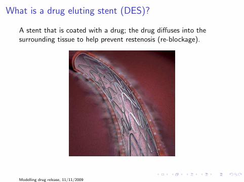
What is a drug eluting stent (DES)?

A stent that is coated with a drug; the drug diffuses into thesurrounding tissue to help prevent restenosis (re-blockage).


Modelling the behaviour of a DES in the body is typically avery formidable challenge

[Yang & Burt, 2006.]


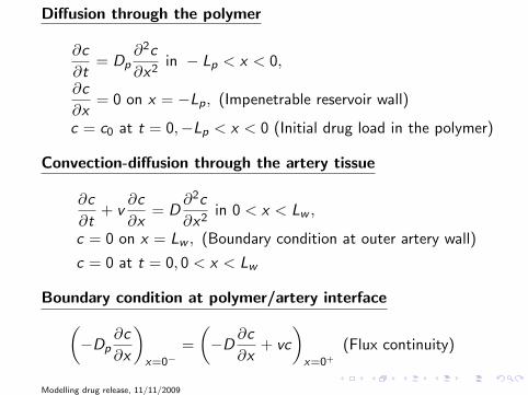
Diffusion through the polymer

∂c

∂t= Dp

∂2c

∂x2in − Lp < x < 0,

∂c

∂x= 0 on x = −Lp, (Impenetrable reservoir wall)

c = c0 at t = 0,−Lp < x < 0 (Initial drug load in the polymer)

Convection-diffusion through the artery tissue

∂c

∂t+ v

∂c

∂x= D

∂2c

∂x2in 0 < x < Lw ,

c = 0 on x = Lw , (Boundary condition at outer artery wall)

c = 0 at t = 0, 0 < x < Lw

Boundary condition at polymer/artery interface

(

−Dp

∂c

∂x

)

x=0−=

(

−D∂c

∂x+ vc

)

x=0+

(Flux continuity)


Swellable polymers

[Siepmann & Siepmann, 2008]


Modelling polymer swelling as a Stefan problem


φ = volume fraction of water.φw = maximum water fraction the polymer can absorb.φc = critical water fraction above which the polymer undergoespolymer chain relaxation.

∂φ

∂t=

∂

∂x

(

D(φ)∂φ

∂x

)

in sw (t) < x < sc(t), t > 0,

φ = φw , D∂φ

∂x=

dsw

dt(1 − φw ) on x = sw (t), t > 0,

φ = φc , D∂φ

∂x= −dsc

dtφc on x = sc(t), t > 0,

sw (0) = sc(0) = 0,

with

D(φ) = D0 exp (βφ) , β > 0. (Fujita-type dependence.)

The conditions for the speeds of the moving boundaries weredetermined using conservation laws.Modelling drug release, 11/11/2009

The problem for the drug concentration can now be posed

With φ(x , t), sw (t), sc(t) calculated, we can now pose the problemfor the drug concentration c(x , t). For example, if the initial drugload in the dry matrix has the constant value c0, and this is belowsolubility, then c(x , t) could satisfy:

∂c

∂t=

∂

∂x

(

D∗(φ)∂c

∂x

)

in sw (t) < x < sc(t), t > 0,

c = 0 on x = sw (t), t > 0,

c = c0 on x = sc(t), t > 0,

withD∗(φ) = D∗

0 exp (β∗φ) , β∗ > 0.


Thermoresponsive polymersPoly(N-isopropylacrylamide) (PNIPAm) is a smart polymer.

◮ In water, it is hydrophilic below 320C (the LCST).◮ Above 320C, it is hydrophobic.◮ These properties can be exploited to create an on/off switch

for drug release.


How to model this?One idea. Let TL be the critical temperature at which thetransition occurs. Write

φw (T ) =

{

φ−w for T < TL

0 for T > TL

with 0 < φ−w < 1, and,

φc(T ) =

{

φ−c for T < TL

1 for T > TL

with φ−w > φ−

c . With these conditions

dsw

dt< 0,

dsc

dt> 0 for T < TL (swelling)

anddsw

dt> 0,

dsc

dt< 0 for T > TL (collapsing)


Documents

Some mathematical models of drug deliveryWhy do we need so many drug delivery systems? Some drug delivery systems Oral - often used for small-molecule cheap drugs, such as aspirin,