Embed Size (px)
Citation preview

Some further studies on improving QFD methodology andanalysisCitation for published version (APA):Raharjo, H. (2010). Some further studies on improving QFD methodology and analysis Eindhoven: TechnischeUniversiteit Eindhoven DOI: 10.6100/IR673463
DOI:10.6100/IR673463
Document status and date:Published: 01/01/2010
Document Version:Publisher’s PDF, also known as Version of Record (includes final page, issue and volume numbers)
Please check the document version of this publication:
• A submitted manuscript is the version of the article upon submission and before peer-review. There can beimportant differences between the submitted version and the official published version of record. Peopleinterested in the research are advised to contact the author for the final version of the publication, or visit theDOI to the publisher's website.• The final author version and the galley proof are versions of the publication after peer review.• The final published version features the final layout of the paper including the volume, issue and pagenumbers.Link to publication
General rightsCopyright and moral rights for the publications made accessible in the public portal are retained by the authors and/or other copyright ownersand it is a condition of accessing publications that users recognise and abide by the legal requirements associated with these rights.
• Users may download and print one copy of any publication from the public portal for the purpose of private study or research. • You may not further distribute the material or use it for any profit-making activity or commercial gain • You may freely distribute the URL identifying the publication in the public portal.
If the publication is distributed under the terms of Article 25fa of the Dutch Copyright Act, indicated by the “Taverne” license above, pleasefollow below link for the End User Agreement:
www.tue.nl/taverne
Take down policyIf you believe that this document breaches copyright please contact us at:
providing details and we will investigate your claim.
Download date: 14. Mar. 2019

SOME FURTHER STUDIES ON IMPROVING QFD METHODOLOGY AND ANALYSIS

SOME FURTHER STUDIES ON IMPROVING QFD METHODOLOGY AND ANALYSIS
HENDRY RAHARJO (B.Eng, Petra Christian University)
A THESIS SUBMITTED
FOR THE DEGREE OF DOCTOR OF PHILOSOPHY
DEPARTMENT OF INDUSTRIAL AND SYSTEMS ENGINEERING
NATIONAL UNIVERSITY OF SINGAPORE
2010

SOME FURTHER STUDIES ON IMPROVING QFD METHODOLOGY AND ANALYSIS
PROEFSCHRIFT ter verkrijging van de graad van doctor aan de Technische Universiteit Eindhoven, op gezag van de rector magnificus, prof.dr.ir. C.J. van Duijn, voor een commissie aangewezen door het College voor Promoties in het openbaar te verdedigen op donderdag 20 mei 2010 om 10.00 uur door Hendry Raharjo geboren te Surabaya, Indonesië

Dit proefschrift is goedgekeurd door de promotoren: prof.dr.ir. A.C. Brombacher en prof.dr. M. Xie Copyright © 2010 by H. Raharjo All rights reserved. No part of this publication may be reproduced, stored in a retrieval system, or transmitted, in any form or by any means, electronic, mechanical, photocopying, recording, or otherwise, without prior written permission of the copyright owner. A catalogue record is available from the Eindhoven University of Technology Library ISBN: 978-90-386-2235-4 NUR 800 Keyword: QFD / AHP / relative priorities / dynamics of relative priorities / future voice of customer / decision making Printed by University printing office, Eindhoven

Acknowledgements
I have been blessed with the opportunity to meet many people to whom I am truly
indebted. First and foremost, I would like to thank my coach, teacher, and also PhD
supervisor, Professor Xie Min. I learnt a lot of things from him, more than just how to
write a good research paper. I recalled that he once said “a smooth ride has nothing to
learn from”; this is particularly true for me since I have never got a smooth ride during the
course of my study. Through many ups and downs, I learnt how to like the things I do
rather than do the things I like, to do things I can rather than do the things I cannot. Those
are some lessons that I learnt from Professor Xie. Words would certainly never suffice to
express my sincere gratitude to him.
I am also honored to have Professor Aarnout C. Brombacher as my PhD supervisor.
His broad knowledge in product development process has guided me to see the big picture
in almost every research work I did. I would like to take this opportunity to sincerely
thank Professor Brombacher for his guidance, patience, support, as well as for providing
me the opportunity to do the research work at TU/e.
During my study, I have also been fortunate to meet Professor Goh Thong Ngee. I
believe that his lecture is one of the most inspiring lectures I have ever attended in my life.
I am grateful for the opportunity and would like to thank Professor Goh for his inspiring
lectures, which always spur his students’ spirit to pursue further knowledge even after the
course is over.
The latter part of this thesis work is carried out while I am working as a researcher at
Chalmers University of Technology. I have been again blessed with the opportunity to
meet my grand supervisor, Professor Bo Bergman. I have to admit that many times I am
simply astonished by his wisdom and critical thoughts. The stay here has been an eye-
opening experience for me, especially with respect to the team-work and social interaction
(Swedish ‘fika’). I am also grateful to meet Dr. Ida Gremyr and family; their kind
hospitality and support is truly appreciated. I would also like to thank my colleagues at
quality sciences division for making my stay so enjoyable and rewarding.
I would like to extend my gratitude to the ISE (NUS) and BPD (TU/e) faculty
members, staffs, and colleagues. Thanks to Jiang Hong, Long Quan, Wu Yanping, Zhu
i

ii
Zhecheng, Aldy Gunawan, and Markus Hartono. Those people and other fellow friends
who I cannot mention their names one by one really make my stay at NUS a memorable
one. Also, thanks to Dr. Jan L. Rouvroye, Dr. Lu Yuan, Jeroen Keijzers, and other fellow
friends at TU/e, from whom I learnt quite many new things.
Before joining NUS, I was quite fortunate to meet Professor Wang Mingzhe of
Huazhong University of Science and Technology (Wuhan, China), Professor Susanti
Linuwih and Dr. Suhartono of Institut Teknologi Sepuluh Nopember (ITS, Indonesia), and
Dr. Hartono Pranjoto of Widya Mandala Catholic University (UKWM, Indonesia). It was
their support and help which encouraged me to embark on this PhD journey. I also remain
thankful to my colleagues and students at Widya Mandala Catholic University (UKWM,
Indonesia) with whom I had worked together for three years.
Finally, I would like to express my deepest appreciation to my father, my mother, and
my sister (Violin) who always support and encourage me in good or bad times. I am fully
aware of the fact that this thesis would have never been completed without the love, care,
and understanding of the flesh of my flesh, Moureen, to whom I owed many inspirations
and to whom I would like to dedicate this work.
H. Raharjo
Gothenburg, August 2009.

TABLE OF CONTENTS ACKNOWLEDGMENTS .............................................................................................. i TABLE OF CONTENTS ............................................................................................ iii SUMMARY ................................................................................................................. viii SAMENVATTING ........................................................................................................ x LIST OF TABLES ....................................................................................................... xii LIST OF FIGURES .................................................................................................... xiv
CHAPTER 1: INTRODUCTION 1.1 Problem background ............................................................................................... 1 1.2 Research questions .................................................................................................. 5 1.3 Objective and delimitation ...................................................................................... 6 1.4 Outline of thesis ...................................................................................................... 8 1.5 Terminology .......................................................................................................... 10
CHAPTER 2: A FURTHER STUDY ON THE USE OF ANALYTIC HIERARCHY PROCESS IN QFD (PART 1 OF 2) – A CASE STUDY
2.1 In what ways does AHP contribute to an improved QFD analysis? ..................... 12 2.2 Using AHP in QFD: An education case study ...................................................... 14 2.2.1 QFD’s use in education and some problematic areas .................................. 14 2.2.2 The proposed methodology .......................................................................... 18 2.2.3 The research design ...................................................................................... 21 2.2.4 The results .................................................................................................... 23 2.2.5 Sensitivity analysis ....................................................................................... 26 2.3 A remark on AHP’s shortcoming ......................................................................... 27 2.4 Conclusion and implication .................................................................................. 28
CHAPTER 3: A FURTHER STUDY ON THE USE OF ANALYTIC HIERARCHY PROCESS IN QFD (PART 2 OF 2) – A GENERALIZED MODEL
3.1 Introduction ........................................................................................................... 31 3.2 The ANP and its use in QFD ................................................................................ 34 3.2.1 The ANP and the AHP ................................................................................. 34 3.2.2 Existing ANP’s use in QFD and its limitations ........................................... 35
iii

3.3 Some important factors in product design using QFD .......................................... 37 3.3.1 New product development (NPD) risk ........................................................ 37 3.3.2 Benchmarking information .......................................................................... 40 3.3.3 Feedback information .................................................................................. 41 3.4 The proposed generalized model .......................................................................... 41 3.4.1 The model .................................................................................................... 42 3.4.2 The model and the HoQ’s components ........................................................ 43 3.4.3 A suggested step-by-step procedure for using the model ............................ 45 3.4.4 Types of questions to elicit decision makers’ judgments ............................ 48 3.4.5 Group decision making using the AHP/ANP .............................................. 49 3.4.6 Fuzziness in the AHP/ANP .......................................................................... 50 3.5 An illustrative example ......................................................................................... 51 3.6 Discussion ............................................................................................................. 62
CHAPTER 4: DEALING WITH THE DYNAMICS OF RELATIVE PRIORITIES: PROPOSING A NEW MODELING TECHNIQUE
4.1 Introduction ........................................................................................................... 65 4.2 Existing approaches and research motivation ....................................................... 67 4.2.1 Shortcoming of Saaty’s time dependent approach ....................................... 67 4.2.1.1 The failure to preserve consistency over time ................................. 68 4.2.1.2 The rigidity of dynamic judgment approach .................................... 70 4.2.2 Limitation of compositional linear trend .................................................... 73 4.2.3 Limitation of the DRHT approach ............................................................... 74 4.3 Compositional data fundamentals ......................................................................... 75 4.3.1 Simplex sample space .................................................................................. 75 4.3.2 Operations in the simplex ............................................................................ 75 4.4 The proposed method: compositional exponential smoothing ............................. 76 4.4.1 General procedure ........................................................................................ 77 4.4.2 Compositional single exponential smoothing (CSES) ................................. 78 4.4.3 Compositional double exponential smoothing (CDES) ............................... 79 4.4.4 Fitting error measurement ............................................................................ 79 4.4.5 Smoothing constant and initialization .......................................................... 80 4.4.6 Ternary diagram ........................................................................................... 81 4.5 An illustrative example ......................................................................................... 81 4.5.1 Model building and forecasting process using four methods ...................... 84 4.5.2 Residual analysis of the four models ........................................................... 87 4.5.3 Solving the case study data using Saaty’s approach .................................... 89 4.6 Discussion and limitations .................................................................................... 92 4.6.1 Dynamic judgments and dynamic priorities ................................................ 92 4.6.2 Short-term and long-term forecast ............................................................... 93 4.6.3 Computation efficiency ................................................................................ 94 4.7 Conclusion ............................................................................................................ 94
iv

CHAPTER 5: APPLICATION OF THE MODELING TECHNIQUE (PART 1 OF 2) – INTEGRATING KANO’S MODEL DYNAMICS INTO QFD
5.1 Introduction ........................................................................................................... 97 5.2 Kano’s model in QFD: existing approaches and research gap ............................. 99 5.2.1 Kano’s model and its dynamics ................................................................... 99 5.2.2 Kano’s model for multiple product design in QFD ................................... 100 5.3 Modeling Kano’s model dynamics ..................................................................... 102 5.3.1 The input .................................................................................................... 102 5.3.2 The CDES method ..................................................................................... 103 5.3.3 Selection of model parameter .................................................................... 104 5.3.4 Fitting error measurement .......................................................................... 105 5.4 Kano optimization for multiple product design .................................................. 105 5.4.1 Deriving weights from the forecasted Kano percentage data .................... 106 5.4.2 Deriving adjusted weights .......................................................................... 107 5.4.3 Deriving DQ importance rating using Kano results .................................. 109 5.4.4 The optimization model ............................................................................. 110 5.5 An illustrative example ....................................................................................... 112 5.5.1 Modeling Kano’s model dynamics ............................................................ 113 5.5.1.1 The input ........................................................................................ 113 5.5.1.2 Selection of model parameter ........................................................ 115 5.5.1.3 Fitting error measurement .............................................................. 115 5.5.1.4 Results’ interpretation .................................................................... 116 5.5.2 Kano optimization for multiple product design ......................................... 117 5.5.2.1 Deriving weights from the forecasted Kano percentage data ....... 119 5.5.2.2 Deriving adjusted weights ............................................................. 119 5.5.2.3 Deriving DQ importance rating using Kano results ..................... 120 5.5.2.4 The optimization model ................................................................ 121 5.6 Conclusion .......................................................................................................... 122
CHAPTER 6: APPLICATION OF THE MODELING TECHNIQUE (PART 2 OF 2) – DYNAMIC BENCHMARKING IN QFD
6.1 Introduction ......................................................................................................... 124 6.2 The need of dynamic benchmarking: literature review and research gap........... 126 6.3 The proposed dynamic benchmarking methodology .......................................... 129 6.3.1 The input .................................................................................................... 129 6.3.2 The step-by-step procedure ........................................................................ 131 6.4 An illustrative example ....................................................................................... 132 6.4.1 The input .................................................................................................... 133 6.4.2 The process ................................................................................................ 135 6.4.3 The output and analysis ............................................................................. 136 6.5 The competitive weighting scheme: A SWOT-based approach ......................... 139 6.6 Conclusion .......................................................................................................... 143
v

CHAPTER 7: A FURTHER STUDY ON QFD’S RELATIONSHIP MATRIX: INVESTIGATING THE NEED OF NORMALIZATION
7.1 Introduction ......................................................................................................... 146 7.2 The QFD relationship matrix: some problems and research gap ........................ 148 7.2.1 Some problems in QFD relationship matrix .............................................. 148 7.2.2 The research gap ........................................................................................ 149 7.3 The pros and cons of normalization in QFD ....................................................... 152 7.3.1 The pros ..................................................................................................... 152 7.3.2 The cons ..................................................................................................... 153 7.4 Some observations and a proposed rule of thumb .............................................. 155 7.4.1 Some observations ..................................................................................... 155 7.4.2 A proposed rule of thumb .......................................................................... 157 7.4.3 A validation example ................................................................................. 159 7.5 Conclusion .......................................................................................................... 163
CHAPTER 8: A FURTHER STUDY ON PRIORITIZING QUALITY CHARACTERISTICS IN QFD
8.1 Introduction ......................................................................................................... 166 8.2 The dynamic QFD (DQFD) model ..................................................................... 168 8.2.1 Why is it important to incorporate customer needs’ dynamics? ................ 168 8.2.2 The DQFD model ...................................................................................... 169 8.2.3 The forecasting technique .......................................................................... 171 8.2.4 Estimation of future uncertainty ................................................................ 172 8.2.5 Decision making ........................................................................................ 173 8.3 The proposed methodology ................................................................................. 174 8.3.1 A step-by-step procedure ........................................................................... 175 8.3.2 Optimization model 1: Utilitarian approach .............................................. 176 8.3.3 Optimization model 2: Non-utilitarian approach ....................................... 179 8.4 An example ......................................................................................................... 182 8.4.1 Using optimization model 1: Utilitarian approach ..................................... 189 8.4.2 Using optimization model 2: Non-utilitarian approach ............................. 193 8.5 Discussion 8.5.1 Selection of forecasting technique ............................................................. 196 8.5.2 A possible implication to development of innovative products ................. 196 8.6 Conclusion .......................................................................................................... 199
CHAPTER 9: CONCLUSION AND FUTURE RESEARCH 9.1 Conclusion .......................................................................................................... 201 9.2 Major contributions ............................................................................................. 202 9.3 A note on the practical implication of DQFD for innovative products .............. 204 9.4 Future research .................................................................................................... 206
REFERENCES ........................................................................................................... 207
vi

vii
Appendix A: Sample of questionnaire to elicit QFD team’s judgments ..................... 216 Appendix B: Judgments results based on arc’s category ............................................ 218 Appendix C: Published commercial specification of Nokia’s 6000s series planned to be introduced in 2007 .......................................................... 220 Appendix D: Published commercial specification of Nokia’s 6000s series planned to be introduced in 2008 .......................................................... 221 Appendix E: Author’s list of publications .................................................................. 222 Curriculum Vitae ....................................................................................................... 223

Summary
Quality Function Deployment (QFD) starts and ends with the customer. In other words,
how it ends may depend largely on how it starts. Any QFD practitioners will start with
collecting the voice of the customer that reflects customer’s needs as to make sure that the
products will eventually sell or the service may satisfy the customer. On the basis of those
needs, a product or service creation process is initiated. It always takes a certain period of
time for the product or service to be ready for the customer. The question here is whether
those customer-needs may remain exactly the same during the product or service creation
process. The answer would be very likely to be a ‘no’, especially in today’s rapidly
changing environment due to increased competition and globalization.
The focus of this thesis is placed on dealing with the change of relative importance of
the customer’s needs during product or service creation process. In other words, the
assumption is that there is no new need discovered along the time or an old one becomes
outdated; only the relative importance change of the existing needs is dealt with.
Considering the latest development of QFD research, especially the increasingly extensive
use of Analytic Hierarchy Process (AHP) in QFD, this thesis aims to enhance the current
QFD methodology and analysis, with respect to the change during product or service
creation process, as to continually meet or exceed the needs of the customer. The entire
research works are divided into three main parts, namely, the further use of AHP in QFD,
the incorporation of AHP-based priorities’ dynamics in QFD, and decision making
analysis with respect to the dynamics.
The first part focuses on the question “In what ways does AHP, considering its
strength and weakness, contribute to an improved QFD analysis?” The usefulness of AHP
in QFD is demonstrated through a case study in improving higher education quality of an
education institution. Furthermore, a generalized model of using AHP in QFD is also
proposed. The generalized model not only provides an alternative way to construct the
house of quality (HoQ), but also creates the possibility to include other relevant factors
into QFD analysis, such as new product development risks.
The second part addresses the question “How to use the AHP in QFD in dealing with
the dynamics of priorities?” A novel quantitative method to model the dynamics of AHP-
viii

based priorities in the HoQ is proposed. The method is simple and time-efficient. It is
especially useful when the historical data is limited, which is the case in a highly dynamic
environment. As to further improve QFD analysis, the modeling method is applied into
two areas. The first area is to enhance the use of Kano’s model in QFD by considering its
dynamics. It not only extends the use of Kano’s model in QFD, but also advances the
academic literature on modeling the life cycle of quality attributes quantitatively. The
second area is to enhance the benchmarking part of QFD by including the dynamics of
competitors’ performance in addition to the dynamics of customer’s needs.
The third part deals with the question “How to make decision in a QFD analysis with
respect to the dynamics in the house of quality?” Two decision making approaches are
proposed to prioritize and/or optimize the technical attributes with respect to the modeling
results. Considering the fact that almost all QFD translation process employs the
relationship matrix, a guideline for QFD practitioners to decide whether the relationship
matrix should be normalized is developed. Furthermore, a practical implication of the
research work towards the possible use of QFD in helping a company develop more
innovative products is also discussed.
In brief, the main contribution of this thesis is in providing some novel methods and/or
approaches to enhance the QFD’s use with respect to the change during product or service
creation process. For scientific community, this means that the existing QFD research has
been considerably improved, especially with the use of AHP in QFD. For engineering
practice, a better way of doing QFD analysis, as a customer-driven engineering design
tool, has been proposed. It is hoped that the research work may provide a first step into a
better customer-driven product or service design process, and eventually increase the
possibility to create more innovative and competitive products or services over time.
ix

Samenvatting
Quality Function Deployment (QFD) begint en eindigt bij de klant. Met andere
woorden het eindresultaat hangt in belangrijke mate af van hoe het proces is gestart. Iedere
QFD gebruiker begint met het verzamelen van de ‘voice of the customer’, die de behoefte
van de klant representeert, opdat het uiteindelijke product wordt verkocht of de dienst de
klant tevreden stelt. Gebaseerd op die behoeftes wordt een product- of service creatie
proces opgestart. Er verloopt altijd enige tijd voordat het product of de service gereed is
voor de klant. De hieraan gerelateerde vraag is op de klanten behoeftes exact hetzelfde
blijven gedurende het product- of service creatie proces. Het antwoord op deze vraag is
zeer waarschijnlijk ‘nee’, vooral vanwege de snel veranderende omgeving als gevolg van
toenemende concurrentie en globalisatie.
De focus van dit proefschrift is hoe om te gaan met de verandering van de mate van
relatieve belangrijkheid van klanten behoeftes gedurende het product- of service creatie
proces. Met ander woorden, de aanname is dat in de loop van de tijd geen nieuwe
behoeftes gevonden worden of bestaande behoeftes niet meer gelden; alleen de mate van
relatieve belangrijkheid van de bestaande behoeftes wordt geadresseerd. Gezien de
recente ontwikkelingen op het gebied van QFD onderzoek, met name de toepassing op
steeds grotere schaal van het Analytic Hierarchy Process (AHP) in QFD, richt dit
proefschrift zich op de verbetering van de bestaande QFD methodologie en bijbehorende
analyse, met betrekking tot de veranderingen gedurende het product- of service creatie
proces, om zodoende aan de behoeftes van de klant tegemoet te komen of deze te
overtreffen. Het hele onderzoek is onderverdeeld in drie delen namelijk het uitgebreidere
gebruik van AHP in QFD, het inbouwen van op AHP prioriteiten gebaseerd dynamisch
gedrag in QFD, en analyse gericht op beslissingen betreffende de dynamische aspecten.
Het eerste gedeelte van het proefschrift is gericht op de vraag “Op welke manier
draagt AHP, gegeven zijn sterktes en beperkingen, bij aan een verbeterde QFD analyse?”.
Het nut van AHP in QFD wordt gedemonstreerd via een case studie betreffende de
verbetering van de kwaliteit van een hoger opleidingsinstituut. Daarnaast wordt ook een
gegeneraliseerd model van de toepassing van AHP in QFD voorgesteld. Dit
gegeneraliseerd model biedt niet alleen een alternatieve methode om het “House of
x

xi
Quality” (HoQ) op te bouwen, maar ook de mogelijkheid om andere relevante factoren
zoals de risico’s rondom de ontwikkeling van een nieuw product in te bouwen.
Het tweede gedeelte van het proefschrift adresseert de vraag “Hoe moet AHP gebruikt
worden in QFD wat betreft de dynamiek in belangrijkheid?” Een nieuwe kwantitatieve
methode om dynamiek in AHP gebaseerde prioriteiten op te nemen in het HoQ wordt
gepresenteerd. De methode is eenvoudig en efficiënt qua tijd. Ze is vooral nuttig in het
geval van beperkte historische data, wat in het bijzonder het geval is in een zeer
dynamische omgeving. Om QFD analyse verder te verbeteren is de methode toegepast op
twee gebieden. Het eerste gebied is het verbeteren van het gebruik van Kano’s model in
QFD voor wat betreft dynamische aspecten. Dit levert tevens een bijdrage aan de
academische literatuur over kwantitatief modelleren van de levenscyclus van
kwaliteitskenmerken. Het tweede gebied is het verbeteren van het “benchmarking” deel
van QFD door het toevoegen van de dynamiek van de prestatie van concurrenten, naast de
dynamiek in behoeftes van klanten.
Het derde gedeelte behandelt de vraag “Hoe kan in een QFD analyse een beslissing
genomen worden met inachtneming van de dynamiek in het House of Quality?”
Gepresenteerd worden twee aanpakken voor het nemen van beslissingen voor het
prioriteren en/of optimaliseren van technische kenmerken. Omdat bijna alle QFD
processen gebruik maken van de relatie matrix, is voor QFD gebruikers een richtlijn
ontwikkeld om te beslissen of de relatie matrix genormaliseerd moet worden. Daarnaast
wordt een praktische toepassing van het onderzoek geadresseerd betreffende mogelijk
gebruik van QFD om een bedrijf te helpen meer innovatieve producten te ontwikkelen.
Samengevat, is de bijdrage van dit proefschrift het aanbieden van nieuwe methodes
en/of benaderingen voor verbetering van QFD gebruik gericht op integratie van
veranderingen gedurende het product of service creatie proces. Voor de wetenschappelijke
gemeenschap is het bestaande QFD onderzoek verbeterd, in het bijzonder voor wat betreft
het gebruik van AHP in QFD. Voor de ontwerppraktijk wordt een betere manier
voorgesteld om een QFD analyse te gebruiken als een klant gedreven ontwerp tool. De
hoop is dat dit onderzoek een eerste stap biedt naar een beter klantgedreven product of
service creatie proces, en uiteindelijk de mogelijkheid vergroot om meer innovatieve en
competitieve producten of services te creëren.
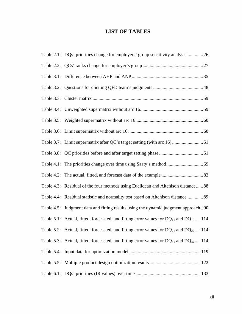
LIST OF TABLES
Table 2.1: DQs’ priorities change for employers’ group sensitivity analysis .............. 26
Table 2.2: QCs’ ranks change for employer’s group ................................................... 27
Table 3.1: Difference between AHP and ANP ............................................................ 35
Table 3.2: Questions for eliciting QFD team’s judgments .......................................... 48
Table 3.3: Cluster matrix ............................................................................................. 59
Table 3.4: Unweighted supermatrix without arc 16 ..................................................... 59
Table 3.5: Weighted supermatrix without arc 16 ......................................................... 60
Table 3.6: Limit supermatrix without arc 16 ............................................................... 60
Table 3.7: Limit supermatrix after QC’s target setting (with arc 16) .......................... 61
Table 3.8: QC priorities before and after target setting phase ..................................... 61
Table 4.1: The priorities change over time using Saaty’s method ............................... 69
Table 4.2: The actual, fitted, and forecast data of the example ................................... 82
Table 4.3: Residual of the four methods using Euclidean and Aitchison distance ...... 88
Table 4.4: Residual statistic and normality test based on Aitchison distance ............. 89
Table 4.5: Judgment data and fitting results using the dynamic judgment approach .. 90
Table 5.1: Actual, fitted, forecasted, and fitting error values for DQ11 and DQ12 ..... 114
Table 5.2: Actual, fitted, forecasted, and fitting error values for DQ21 and DQ22 ..... 114
Table 5.3: Actual, fitted, forecasted, and fitting error values for DQ31 and DQ32 ..... 114
Table 5.4: Input data for optimization model ............................................................ 119
Table 5.5: Multiple product design optimization results ........................................... 122
Table 6.1: DQs’ priorities (IR values) over time ....................................................... 133
xii

xiii
Table 6.2: Customer competitive assessment over time for DQ1 .............................. 134
Table 6.3: Customer competitive assessment over time for DQ2 .............................. 134
Table 6.4: Customer competitive assessment over time for DQ3 .............................. 135
Table 6.5: The proposed competitive weighting scheme ........................................... 141
Table 6.6: The determination of final DQs’ priority .................................................. 142
Table 7.1: HoQ example when normalization is desirable: before normalization .... 152
Table 7.2: HoQ example when normalization is desirable: after normalization ....... 153
Table 7.3: HoQ example when normalization is undesirable: before normalization ................................................................................. 154 Table 7.4: HoQ example when normalization is undesirable: after normalization ... 155 Table 7.5: HoQ of combined model for the basic product before normalization ...... 160 Table 7.6: HoQ of combined model for the basic product after normalization ......... 160 Table 7.7: HoQ of combined model for the high-end product before normalization ................................................................................. 162 Table 7.8: HoQ of combined model for the high-end product after normalization ... 162 Table 8.1: Actual, fitted, forecasted, and fitting error values of all IR ...................... 184 Table 8.2: Descriptive statistics and normality test of forecasting residual .............. 185 Table 8.3: Mean value test of forecasting residual .................................................... 185 Table 8.4: Independence test of forecasting residual ................................................. 186 Table 8.5: Optimization results with SD constraint ................................................... 192 Table 8.6: Optimization results without SD constraint .............................................. 193 Table 8.7: Example of customer preference dynamics from commercial specification .............................................................................................. 198

LIST OF FIGURES
Figure 1.1: Time-lag problem when using QFD ............................................................ 2
Figure 1.2: Dynamics in the House of Quality .............................................................. 4
Figure 1.3: Illustration for customer’s needs’ relative priorities dynamics ................... 5
Figure 1.4: Organization of the thesis ............................................................................ 8
Figure 2.1: The proposed methodology of using AHP in QFD ................................... 21
Figure 2.2: An example of students’ group hierarchy ................................................. 23
Figure 2.3: Trimmed part of HoQ for students’ group ................................................ 24
Figure 2.4: Trimmed part of HoQ for lecturers’ group ................................................ 24
Figure 2.5: Complete HoQ for employers’ group ........................................................ 25
Figure 3.1: The proposed ANP framework for QFD ................................................... 43
Figure 3.2: Network model for the example ................................................................ 53
Figure 4.1: Consistency Ratio (CR) values over time using Saaty’s method .............. 70
Figure 4.2: Ternary diagram of Saaty’s method (Saaty, 2007) .................................... 71
Figure 4.3: Ternary diagrams of a random AHP matrix with 1000 replications using pre-specified CR range .................................................................... 72 Figure 4.4: Ternary diagram of the relative priorities change over 12 periods ........... 82
Figure 4.5: Ternary diagram of fitting historical data using four methods (a-d) ......... 85
Figure 4.6: Plot of actual, fitted and forecasted priorities using the DRHT and the CDES method ............................................................. 87 Figure 4.7: (a) Plot of actual, fitted and forecasted judgments values using Saaty's approach, (b) Ternary diagram of actual, fitted, and forecasted priorities using Saaty’s approach ............................................. 91 Figure 5.1: Graph of actual, fitted, and forecasted values for DQ11 and DQ12 .......... 116
xiv

xv
Figure 5.2: Graph of actual, fitted, and forecasted values for DQ21 and DQ22 .......... 116 Figure 5.3: Graph of actual, fitted, and forecasted values for DQ31 and DQ32 .......... 117 Figure 6.1: Graphical plot of the actual, fitted, and forecasted values of the DQs’ priorities ................................................................................... 136 Figure 6.2: Graphical plot of the actual, fitted, and forecasted values of the customer competitive assessment priorities for DQ1 ........................ 137 Figure 6.3: Graphical plot of the actual, fitted, and forecasted values of the customer competitive assessment priorities for DQ2 ........................ 137 Figure 6.4: Graphical plot of the actual, fitted, and forecasted values of the customer competitive assessment priorities for DQ3 ........................ 137 Figure 6.5: The radar diagram portraying the future competitive assessment ........... 138 Figure 6.6: The proposed weighting scheme ............................................................. 141 Figure 7.1: Pareto chart of combined model for the basic product ............................ 161 Figure 7.2: Pareto chart of combined model for the high-end product ...................... 163 Figure 8.1: The DQFD model .................................................................................... 170 Figure 8.2: Simplified HoQ for employers of graduates ........................................... 183 Figure 8.3: Graphical plot of the actual, fitted, and forecasted importance rating values ......................................................................... 187 Figure 8.4: The DQFD for the employers of graduates ............................................. 188 Figure 8.5: Plot of CDF of all QCs ............................................................................ 189

Chapter 1: Introduction
CHAPTER 1
INTRODUCTION
“The customers of tomorrow will have needs and expectations different from those of our present customers.
For this reason, it is important to keep up with changing needs and expectations, and to learn how to meet
these…” (Bergman and Klefsjö, 2003: quality from customer needs to customer satisfaction)
“Indeed a Critical-to-Quality (CTQ) valid today is not necessarily a meaningful one tomorrow; shifting
social, economic and political scenes would make it imperative that except for immediate, localized projects,
all CTQs should be critically examined at all times and refined as necessary” (Goh, 2002: a strategic
assessment of six sigma)
1.1 Problem Background
Quality Function Deployment (QFD) was first developed in the late 1960s by
Professor Yoji Akao and Shigeru Mizuno. It was motivated by two issues (Akao and
Mazur, 2003). First, it is the importance of design quality. Second, the need to deploy,
prior to production startup, the important quality assurance points needed to ensure the
design quality throughout the production process. According to Akao (1990), as one of the
main founders, QFD can be defined as “a method for developing a design quality aimed at
satisfying the customer and then translating the customer’s demand into design targets and
major quality assurance points to be used throughout the production phases”.
QFD has become a quite popular tool in customer-focused product creation or
development process. Some main benefits of using QFD may include better
communication of cross-functional teamwork, lower project and product cost, better
product design, and increased customer satisfaction (Hauser and Clausing, 1988; Griffin
and Hauser, 1992; Hauser, 1993; Presley et al., 2000; Chan and Wu, 2002a; Xie et al.,
2003). As with any other tools, QFD also has some limitations apart from its benefits. It is
1

Chapter 1: Introduction
limited in the sense that it is more effective for developing incremental products as
opposed to really new products (Griffin, 1992). It is also found that the QFD’s use might
be a bit burdensome due to the incredibly big matrices (Den Ouden, 2006). Furthermore, a
quite recent empirical study also found that QFD does not shorten time-to-market (Lager,
2005).
Nevertheless, taking into account its limitations, QFD does still provide a more
systematic and effective approach to create higher customer satisfaction by bringing a
product or service that the customer wants. In essence, QFD starts and ends with the
customer. By employing QFD, everyone involved in every stage of product or service
creation process may be able to see how the job one is doing can contribute to the chief
end goal, namely, to meet or exceed the end customer’s needs. Such mechanism is a good
way to make sure that the products will eventually sell.
One important key factor for successful application of QFD is the accuracy of the
main input information, namely, the Voice of Customer (VOC) (Cristiano et al., 2001). It
is known that it always takes some time from the time when the customer’s voice is
collected until the time when the product is ready to be launched, as shown in Figure 1.1.
Start
CUSTOMER
Collect VOC Design Process Production Other phases ... Product Purchase... ... ... ...
EndCUSTOMER
QFD
Time Lag
Figure 1.1 Time-lag problem when using QFD
The time-lag duration may certainly vary from one product to another. For example, if it
takes one year time, then the question is whether the product which is about to be
launched may still meet the customer’s needs since it is created based on the customer
2

Chapter 1: Introduction
voice which was collected one year ago. The answer to this question is very likely to be a
‘no’ in the context of today’s rapidly changing market. This, at the same time, assumes
that the rate of change is shorter than or the same as the length of product or service
creation time, for example, the rate of change is yearly and the product or service creation
time is one year or longer.
In the existing QFD literature, there has been too little research devoted into dealing
with the change of customer’s needs during product or service creation process. What
have been done in the literature to tackle such change is to use two types of approaches,
namely, sensitivity analysis (Xie et al., 1998) and forecasting techniques (Shen et al., 2001;
Xie et al., 2003; Wu et al., 2005; Wu and Shieh, 2006). Considering the development of
QFD research in recent years, particularly the increasingly extensive research on the use
of the Analytic Hierarchy Process (AHP)1 in the QFD (Carnevalli and Miguel, 2008; Ho,
2008), those approaches might no longer be effective. Furthermore, almost all of the
previous approaches, which employ forecasting techniques, only rely on a single point
estimate of forecast.
This thesis is written based on a collection of the author’s scientific journal
publications (see Appendix E) which attempts to provide further studies on the methods or
approaches in QFD with respect to the dynamics of QFD’s input information during
product or service creation process. Specifically, the focus is placed on the two elements
in the house of quality (Figure 1.2), namely, the customer’s voice (left wing) and the
competitive benchmarking information (right wing). Those two parts are most likely
1 In 2007, the inventor of AHP (Thomas L. Saaty) was awarded the Akao Prize for the remarkable contribution of AHP in QFD (http://www.qfdi.org/who_is_qfdi/akao_prize.html)
3

Chapter 1: Introduction
subject to change over time since they are obtained externally from the customer’s
judgment or assessment.
Whats/
Demanded Quality
Correlation Matrix
Hows/ Quality Characteristic
Relationship Matrix
Planning Matrix/
Customer Competitive Assessment
Technical Matrix
Figure 1.2 Dynamics in the House of Quality
The entire research works are divided into three focal parts, namely, the further use of
AHP in QFD, the incorporation of AHP-based priorities’ dynamics in QFD, and decision
making analysis with respect to the dynamics. Note that the term ‘dynamic’ is interpreted
as the change over time throughout the thesis (see Section 1.5). It is worth highlighting
that the dynamics that this thesis discusses is the change of relative priorities, which are
obtained using the AHP, over time. The word ‘relative’ here implies that the priorities are
dependent on a certain condition set by the people at a certain place and time. In other
words, those priorities will definitely not remain exactly the same at all time.
An illustrative example of how the relative priorities of three different customer-
needs or demanded qualities (DQs) change during eight periods is shown in Figure 1.3.
The w1, w2, w3, respectively denote the relative weights (priorities) of DQ1, DQ2, and DQ3.
The priorities of the needs may reflect the relative importance or customer’s preference of
the needs. Note that the three DQs themselves have already existed from the beginning of
the analysis. The only change is their relative priorities or importance over time. In
addition, the sum of the priorities of the three DQs for every period is always one (100%).
4

Chapter 1: Introduction
Figure 1.3 Illustration for customer’s needs’ relative priorities dynamics
1.2 Research Question
Reflecting upon the existing QFD literature and the problem described in Section 1.1,
the following main research question is formulated:
Main research question: How to enhance the current QFD methodology and analysis,
especially when the AHP is used in QFD, with respect to the dynamics during product
or service creation process as to continually meet or exceed the needs of the customer?
To answer the above question, three more specific sub-questions are formulated with
respect to the current use of AHP in QFD, the incorporation of AHP-based dynamics into
the house of quality (HoQ), and how to make decision with respect to such dynamics.
Sub-question 1: In what ways does AHP, considering its strength and weakness,
contribute to an improved QFD analysis? The AHP has been widely accepted as a
realistic, flexible, simple, and yet mathematically rigorous modeling technique in multiple
criteria decision making (MCDM) field. A recent survey found that the growth of AHP-
related publications has been enormous during the last three decades (Wallenius et al.,
2008). However, as with any other tool, the AHP is also plagued with shortcomings, such
as, the rank reversal phenomenon and the exponentially growing number of pairwise
comparisons as the number of alternatives being compared gets larger (Raharjo and Endah,
5
Chapter 1: Introduction
2006; Wang et al.,1998). Considering its strength and weakness, this thesis will attempt to
answer the above question by not only explaining the ways AHP may contribute to an
improved QFD analysis, but also providing a better or generalized use of AHP in QFD.
Sub-question 2: How to use the AHP in QFD in dealing with the dynamics of
priorities? The QFD-AHP combination is found to be one of the most popular tools in the
QFD and/or integrated AHP literature in recent years (Ho, 2008; Carnevalli and Miguel,
2008). The term ‘integrated AHP’ is used to refer to other techniques used in combination
with the AHP (Ho, 2008). Most researchers use the AHP to derive the relative importance
of customer’s needs (Armacost et al., 1994; Lu et al., 1994; Park and Kim, 1998; Köksal
and Eğitman, 1998; Zakarian and Kusiak, 1999; Kwong and Bai, 2003; Raharjo et al.,
2007, 2008; Li et al., 2009). Unfortunately, there is almost no study that deals with the
dynamics of AHP-based priorities.
Sub-question 3: How to make decision in a QFD analysis with respect to the
dynamics in the house of quality? This question is a continuation of sub-question 2. The
focus is on how to make decision, with respect to the change of AHP-based priorities in
the HoQ during products or service creation process, as to continually meet or exceed the
needs of the customer. This question may be divided into two smaller questions. One is
how to use the priorities’ dynamics modeling results as the input of the decision model,
and the other is what kind of decision making models that can be used.
1.3 Objective and Delimitation
In general, the main objective of this thesis is to develop novel methods and/or
approaches for enhancing the use of QFD, especially in combination with the AHP, in
6

Chapter 1: Introduction
dealing with the dynamics during product creation process. It is expected that those
methods or approaches, in the long run, may increase the possibility to create innovative
and competitive products or services. In particular, this thesis aims to achieve the
following three specific objectives based on the three research sub-questions:
1. To demonstrate the usefulness as well as to provide a better use of the AHP in QFD.
2. To develop a novel method to model the dynamics of AHP-based priorities in the
house of quality.
3. To develop methods and/or approaches for decision making with respect to the
modeling results as to continually meet or exceed the needs of the customer.
Delimitation of the first objective: The usefulness and better use of the AHP in QFD is
delimited to only the first matrix, namely, the house of quality. A real-world case study in
education will be used to demonstrate the usefulness, and one empirical example based on
interview and questionnaire will be used to show how to use AHP better in QFD.
Delimitation of the second objective: The novel method to model the dynamics of AHP-
based priorities in the house of quality is only applied to two parts of the HoQ. One is in
the customer-needs’ priorities (importance rating part), and the other is in the priorities of
competitive assessment of customer’s needs (competitive benchmarking part). It is also
delimited to the fact that it does not include the case of when a new customer need should
be added or an old one should be removed along the time, although it may be common in
practice. In other words, it only deals with the change of the relative priorities over time.
7

Chapter 1: Introduction
Delimitation of the third objective: The focus is delimited to the translation process and
the decision making analysis using the modeling results. With respect to the translation
process, it is not the objective of this thesis to elaborate how a customer need gets
translated into a specific design or technical attribute, but rather how to use the
relationship matrix in the HoQ to obtain the priorities of the technical attributes properly.
The decision making analysis is delimited to two kinds of optimization model; one
employs a utilitarian approach and the other employs a non-utilitarian approach.
1.4 Outline of the thesis
This thesis is comprised of nine chapters. Chapter 1 provides the problem background,
research questions, objectives, delimitations, outline, and terminologies used in the thesis.
Chapter 2 to Chapter 8 contains the main contributions of the thesis which is derived from
the author’s scientific publications (Appendix E). Chapter 9 concludes the thesis with the
summary of main contributions and possible future research. With respect to the three sub-
questions, the chapters are organized as depicted in Figure 1.4.
Sub‐question1 Sub‐question2 Sub‐question3
Research Question
Chapter2 Chapter3 Chapter4
Chapter5 Chapter6
Chapter7
Chapter8
Figure 1.4 Organization of the thesis
8

Chapter 1: Introduction
Chapter 2 and Chapter 3 will address the first research sub-question that corresponds
to the first specific objective. Chapter 2 will discuss the ways AHP may contribute to an
improved QFD analysis based on the literature. Then, a real-world case study of QFD
application in improving education quality is described. This is to substantiate the
usefulness of AHP in QFD. The need to incorporate the dynamics of customer’s needs in
QFD is also indicated in Chapter 2. Chapter 3 provides a better use of the AHP in QFD
via the generalized form of the AHP, namely, the Analytic Network Process (ANP).
Finally, a remark on the AHP’s shortcoming when the number of alternatives being
compared gets larger is provided.
Chapter 4 will address the second research sub-question which corresponds to the
second specific objective. A novel technique to model the dynamics of AHP-based
priorities is proposed. The proposed modeling technique is applied to two areas as to
advance the QFD literature. The first area (Chapter 5) is in enhancing the use of Kano’s
model in QFD. Based on the recent advancement, a systematic methodology to
incorporate Kano’s model dynamics in QFD is suggested. The second area (Chapter 6) is
in enhancing the benchmarking part of QFD, that is, by including the dynamics of
competitors’ performance in addition to the dynamics of customer’s needs.
Chapter 8 will address the third research sub-question which corresponds to the third
specific objective. Before proceeding to the decision making analysis (Chapter 8), Chapter
7 will first discuss an important issue in the relationship matrix. This is owing to the fact
that the relationship matrix is almost always used in deriving the technical attributes’
priorities, which are the main output of the HoQ. Chapter 8 will propose a systematic
methodology, using the case study in Chapter 2, to incorporate the dynamics of DQs’
priorities into the decision making analysis in the QFD. Two kinds of approaches are
9

Chapter 1: Introduction
proposed to prioritize and/or optimize the technical attributes with respect to the future
needs of the customer. The results from Chapter 5 and Chapter 6 may also be used in
combination with the proposed methodology. A practical implication of the research work
towards the possible use of QFD in helping a company develop more innovative products
will also be discussed.
Chapter 9 concludes the thesis and provides a summary of the major contributions.
Some directions for the extension of the current research are described. It is expected that
the entire study in this thesis may provide a first step to better use QFD with respect to the
change of customer needs’ importance and their competitive assessment during product or
service creation process.
1.5 Terminology
This section provides the important terminologies used in this thesis. The purpose here
is to provide clearly defined terms and to avoid misinterpretation of the meaning. There
are seven important terminologies used throughout this thesis.
• demanded quality (DQ) – this term is used to refer to customer’s needs, attributes, or
requirements. It is also known as the ‘Whats’ in the HoQ. In this thesis, this DQ is
used interchangeably with the voice of the customer (VOC). Note that the essential
different between these two is in the formulation of the language, the VOC is derived
from the customer’s daily language, while the DQ is more formal or specific.
• quality characteristic (QC) – this term is used to refer to the design attributes or
parameters, or the technical/engineering attributes. It is also known as the ‘Hows’ in
the HoQ.
10

Chapter 1: Introduction
11
• priority – this term is used to represent the weight assigned to a specific attribute, for
example, the weight of a DQ or a QC. This weight or priority refers to relative priority
that is obtained from the AHP. It is also used to represent the relative competitive
assessment of a DQ.
• DQ’s priority – In this thesis, this refers to the relative weight assigned to a DQ. It
also refers to the importance rating value (IR value) of the DQ.
• QC’s priority – This refers to the final relative weight of a QC which will usually be
used in an optimization framework.
• dynamics – this word is used to refer to the change over time. In this thesis there are
two types of dynamics. One is the dynamics in the DQs’ priorities and the other is the
dynamics in the DQs’ competitive assessment.
• QFD team – This term is used to refer to a number of people from various functional
groups who together use QFD. It is also used to refer to QFD users or QFD
practitioners.

Chapter 2: A further study on the use of AHP in QFD – A case study
CHAPTER 2
A FURTHER STUDY ON THE USE OF AHP IN QFD (PART 1 OF 2) –
A CASE STUDY
The purpose of this chapter is to provide the first part of a possible answer to the research
question “In what ways does AHP, considering its strength and weakness, contribute to an
improved QFD analysis?” Based on the literature, five reasons that may justify the AHP
as an effective tool to derive DQs’ priorities are identified (Section 2.1). To further
substantiate the contribution of AHP in QFD, a real-world case study demonstrating the
usefulness of AHP in QFD for improving higher education quality of an engineering
department is provided (Section 2.2). A remark on AHP’s shortcoming, when the number
of alternatives being compared gets larger, is provided (Section 2.3). Finally, as an
implication of the case study, it is concluded that there is a need to anticipate the change
of customer’s needs over time as to provide a better strategic planning for the education
institution. A large part of this chapter is reproduced from the author’s two journal papers1.
2.1 In what ways does AHP contribute to an improved QFD analysis?
Two recent reviews (Ho, 2008; Carnevalli and Miguel, 2008) found that the QFD-AHP
combination is one of the most popular tools used in the QFD and/or integrated AHP in
recent years. Most of the researchers use the AHP in QFD to obtain the importance rating
values of the DQs (Armacost et al., 1994; Lu et al., 1994; Park and Kim, 1998; Köksal and 1 Raharjo, H., Xie, M., Goh, T.N., Brombacher, A.C. (2007), A Methodology to Improve Higher Education Quality using the Quality Function Deployment and Analytic Hierarchy Process, Total Quality Management & Business Excellence, 18(10), 1097-1115.
Raharjo, H., Endah, D. (2006), Evaluating Relationship of Consistency Ratio and Number of Alternatives on Rank Reversal in the AHP, Quality Engineering, 18(1), 39-46.
12

Chapter 2: A further study on the use of AHP in QFD – A case study
Eğitman, 1998; Zakarian and Kusiak, 1999; Kwong and Bai, 2003; Raharjo et al., 2007;
Li et al., 2009).
Based on the literature, it can be concluded that there are at least five reasons that
make the AHP an effective way to derive the DQs’ priorities.
1. It provides ratio scale priorities (Harker and Vargas, 1987). The ratio scale priorities
are of great importance to the QFD results due to the fact that only in this type of
scale can the QCs’ priorities be meaningful (Burke et al., 2002), especially when it is
dovetailed with an optimization analysis. Another simple reason for the significance
of ratio scale is the computation in the HoQ which involves multiplication operations,
in which other type of scale, such as ordinal or interval scale (Stevens, 1946) is not
meaningful.
2. It allows the quantified judgments to be tested on their inconsistency, which is not the
case when using the traditional way, such as a rating system of 1 to 5 (Lu et al., 1994;
Armacost et al., 1994).
3. It avoids ‘all things are important’ situation. Chuang (2001) found that the traditional
way, which employs a set of absolute values, such as 1 to 5, might very likely lead to
a tendency for the customers to assign values near to the highest possible scores, and
thus result in somewhat arbitrary and inaccurate QCs’ priorities.
4. Its internal mechanism allows the subjective knowledge or judgments of the QFD
team to be systematically quantified (Raharjo et al., 2008). One example is the use of
the AHP’s hierarchical structure that corresponds to the use of affinity diagram or tree
diagram for structuring the VOC (Raharjo et al., 2007).
5. It provides an exceptional way in effectively facilitating group decision making (Bard
and Sousk, 1990; Dyer and Forman, 1992; Zakarian and Kusiak, 1999)
13

Chapter 2: A further study on the use of AHP in QFD – A case study
Hence, it is evidently clear that the AHP, according to the literature, can be considered as
a beneficial tool in QFD for obtaining DQs’ priorities. In the next section, the above five
reasons will be empirically substantiated by a case study.
2.2 Using AHP in QFD: An education case study
The objective of this case study is to apply the QFD-AHP approach in a systematic
fashion to improve higher education quality in an industrial engineering department. Most
of the contents in this section are reproduced from Raharjo et al. (2007). In the following
subsections, a literature review on the use of QFD in education will be provided and
followed with some existing technical and practical problems which motivated the
research (Section 2.2.1). Afterwards, a methodology to systematically use QFD-AHP for
improving higher education quality is proposed using a step-by-step procedure and a
flowchart (Section 2.2.2). A real-world case study is used to demonstrate the usefulness of
the methodology (Section 2.2.3). Based on the results of the case study, a sensitivity
analysis is suggested to deal with the dynamics of customer’s needs (Section 2.2.4 and
Section 2.2.5). Lastly, a brief conclusion and implication of the study is provided (Section
2.4).
2.2.1 QFD’s use in education and some problematic areas
Since 1980s, higher education institutions have begun to adopt and apply quality
management to the academic domain owing to its success in industry (Grant et al., 2002)
and they have also benefited from the application of TQM (Kanji and Tambi, 1999; Owlia
and Aspinwall, 1998). QFD, as one of the most useful TQM tools, has also been used
14

Chapter 2: A further study on the use of AHP in QFD – A case study
quite extensively in academia. Jaraiedi and Ritz (1994) applied QFD to analyze and
improve the quality of the advising and teaching process in an engineering school. Köksal
and Eğitman (1998) used QFD to improve industrial engineering education quality at the
Middle East Technical University. Lam and Zhao (1998) suggested the use of the QFD
and the AHP to identify appropriate teaching techniques and to evaluate their
effectiveness in achieving an education objective. Bier and Cornesky (2001) critically
analyzed and constructed a higher education curriculum to meet the needs of the
customers and accrediting agency using QFD.
Adopting the constructivist’s point of view, Chen and Chen (2001) introduced a
QFD-based approach to evaluate and select the best-fit textbook based on the VOC.
Kauffmann et al. (2002) also used the QFD to select courses and topics that enhance a
master of engineering management program effectiveness. They further pointed out the
additional benefit of QFD in the academic context, that is, to develop collegial consensus
by providing an open and measurable decision process. Brackin (2002) wrote the analogy
of the use of QFD in the industry with the assessment of engineering education quality by
breaking down the assessment items into a set of WHATs and HOWs following the four
phases of QFD. Duffuaa et al. (2003) applied the QFD for designing a basic statistics
course. More recently, Sahney et al. (2004, 2006) used the QFD, in combination with
SERVQUAL as well as Interpretive Structural Modeling and Path Analysis, to identify a
set of minimum design characteristics to meet the needs of the student as an external
customer of the educational system. Chen and Yang (2004) explored the possibility to use
Internet technology by developing a Web-QFD model. They gave a real-world example of
an education system in Taiwan and argued that the Web-QFD may not only provide a
more efficient way of using the QFD in terms of cost, time and territory, but also may
15
Chapter 2: A further study on the use of AHP in QFD – A case study
facilitate better group decision making process. Aytaç and Deniz (2005) used the QFD to
review and evaluate the curriculum of the Tyre Technology Department at the Kocaeli
University Köseköy Vocational School of Higher Education.
It is clear that QFD has been extensively used in improving education quality.
However, if one takes a closer look at how QFD was implemented in education, one may
discover some problematic areas that need improvement. In this section, five major
problems will be highlighted. They can be divided into two major categories, namely, the
technical problems (the first, the second, and the third problems) and the practical ones
(the fourth and the fifth problems).
The first problem is the use of absolute values for DQs’ priorities. As pointed out by
Chuang (2001), the customers will tend to assign a high degree of importance to most of
their requirements, thus resulting in values near the highest possible score. These values
will have no significant meaning (Cohen, 1995) and will later produce somewhat arbitrary
and inaccurate results for prioritizing QCs. Some examples for using a set of discrete
values can be found in Jaraiedi and Ritz (1994), Ermer (1995), Chen and Chen (2001),
Kaminski (2004), and Chou (2004). Therefore, relative measurement for assessing the
importance of customer requirements is suggested as a better alternative.
The second problem is the technique that is used to obtain priorities of a group’s
preference. Some of the studies simply proposed the use of an arithmetic mean or
weighted arithmetic mean for obtaining the preference of the customer group, which
seems arbitrary and not robust. This case can be found in Bier and Cornesky (2001),
Hwarng and Teo (2001), Duffuaa et al. (2003), Kaminski et al. (2004), or Aytaç and Deniz
(2005). A better approach would be to use a geometric mean that also formed the
16

Chapter 2: A further study on the use of AHP in QFD – A case study
foundation of a group preference method in the AHP (Ramanathan and Ganesh, 1994;
Forman and Peniwati, 1998).
The third problem is the difficulty in identifying a true relationship between DQs and
QCs. It seems quite unrealistic if all DQs are related to all QCs so that the QFD
relationship matrix will be full blocked. It may imply that the QFD team has difficulty in
assigning more discriminating relationship values between them. Examples of this case
can be found in Duffuaa et al. (2003) or Lam and Zhao (1998), which used a full blocked
relationship matrix.
The fourth problem is that the flexibility in using QFD in education should be
enhanced, resting on the assumption that it is not just a “plug-and-play decision machine”
(see Govers, 2001). There are two points to highlight. First, the number of matrices does
not have to be strictly four (Hauser and Clausing, 1988). Based on the necessity of the
deployment process, the QFD team may decide how many matrices or houses to use. An
example given by Brackin (2002) to follow the four phases showed the inflexibility.
Second, the true VOC should come from the proper and right customers. Several
researchers in education do not include the students since they may have unnecessary
wants and be considered too immature to judge the content of education. On the other
hand, Sa and Saraiva (2001) attempted to include kindergarten children as the customers.
This approach seems to be overconfident and risky.
The fifth problem lies in pooling the needs of several different customers into one
group. This might possibly lead to a fallacious conclusion since one stakeholder may have
a unique need which others may not consider, or even a conflicting need with respect to
other customers. An example for this case can be found in Köksal and Eğitman (1998)
17

Chapter 2: A further study on the use of AHP in QFD – A case study
which combined three different stakeholders into one. If the number of DQs and QCs is
not very large, each customer group may be treated separately using one HoQ.
Therefore, in view of these problems, this section attempts to fill in the gap by
providing a better methodology of using AHP and QFD to improve higher education
quality. It is hoped that this will help higher education institutions, in general, improve
their quality in the future by providing a better education program for their nation.
2.2.2 The proposed methodology
The aim of the methodology is to use the QFD-AHP approach in a more systematic
fashion in order to improve higher education quality of an industrial engineering
department, taking into account the need to overcome the technical and the practical
problems mentioned above. Here, the AHP will be used to obtain relative measurement,
obtain group preference, and check the inconsistency of decision makers’ judgments. A
method proposed by Nakui (1991) was employed to ensure that no superfluous DQs or
QCs are included while still maintaining the significant relationships among DQs and QCs.
Each of the customers uses a separate HoQ. Note that the number of matrices or houses
used can be adjusted according to the need of the deployment process. In the case study,
only the first house of quality is used.
A step-by-step approach of the methodology is presented below. This procedure
applies for each customer group. A flowchart of the step-by-step procedures can be seen in
Figure 2.1.
Step 1. Conduct a pilot survey of customer needs. In other words, this is an in-the-field
observation in order to collect the VOC from the true source of information. A
variety of methods, such as contextual inquiry, direct observation, focus group,
18

Chapter 2: A further study on the use of AHP in QFD – A case study
questionnaires, and so on, can be employed. After the survey, the QFD team
should sort out and organize the preliminary results. This will help the QFD team
see the big picture of the customers’ needs.
Step 2. Conduct one-on-one in-depth interview with the customers. In this step, adopting
the Garbage-In-Garbage-Out (GIGO) philosophy, it is very crucial to select some
knowledgeable decision makers which are also representative to each of the
groups involved. Note that it is important to select the right students to be
interviewed in order to avoid unnecessary and self-centered wants.
Step 3. Use affinity diagram to classify or sort out the DQs and construct a hierarchy
based on the grouping. The higher the hierarchy, the less the effort to obtain the
DQs’ priorities. This hierarchy also serves as the AHP hierarchy.
Step 4. Explore each DQ hierarchically by a tree diagram and translate it into an
appropriate QC. The QC is defined as the strategy or way to achieve the DQ. One
DQ may be related into some QCs, and vice versa.
Step 5. Verify whether the DQs and the respective QCs are valid, otherwise, the QFD
team should carry out the interview again.
Step 6. Ask the selected decision makers to make the AHP pairwise comparisons in order
to derive the priorities of the DQs. The QFD team may explain to decision
makers who are not familiar with the AHP mode of questioning.
Step 7. Obtain group preference using geometric mean approach (Forman and Peniwati,
1998). Then, check whether there is a need to resurvey the decision makers
owing to inconsistent judgments. The Expert Choice software can be used to
obtain the priorities of DQs as well as to do the inconsistency check.
19

Chapter 2: A further study on the use of AHP in QFD – A case study
Step 8. Construct the HoQ of each customer group. The minimum set of constructing the
HoQ should exist, such as the DQs and their priorities, the QCs and their
priorities. Other components (e.g. the roof, competitive assessment) might be
added as necessary. The Microsoft-Excel software would be a good alternative to
do the HoQ analysis.
Step 9. Verify the completed HoQ components. Some rules to check the relationship
matrix as proposed by Nakui (1991) can be used. For example, if a DQ has no
corresponding QC at all, then this DQ should be taken away.
Step 10. Compute the QCs’ priorities, and obtain their rankings. The QFD team may
evaluate whether there is a need to extend the deployment process by using
another matrix or house. If there is a need to use another matrix, a similar process
can again be conducted (Step 8).
Step 11. Conduct sensitivity analysis to provide a sense of how robust is the decision made
by the QFD team if there is a change in the input data. This is also useful to
anticipate future needs of customer and variability in the DQs.
Step 12. Other downstream analysis, such as gap analysis, SWOT analysis, and so forth,
can be added accordingly.
20

Chapter 2: A further study on the use of AHP in QFD – A case study
Figure 2.1 The proposed methodology of using AHP in QFD
STARTA
Pilot survey of
2.2.3 The research design
The case study was carried out as a final year project at the department. The
customers of the department are divided into two major groups, namely, the internal
(lecturers and students) and the external customer (employers of the graduates). The data
collected from the students’ group comprised of several representative students from each
customer needs
One-on-onecustomer interview
Use affinity diagram toconstruct DQs hierarchy
Use tree diagram to listthe QCs
Use AHP pairwise comparison
of each customer’s DQsto derive importance rating
Obtain grouppreference
Consistent?(CR <=10%)
Yes
No
Resurveythe
customer
Construct HoQ
Verified?Valid?
Yes
No
Verified?Nakui (1991)
No Check HoQrel. matrix
(QFD team)
Derive QCs' priorities
Yes
A
Subsequent/ downstream analysis(gap analysis, SWOT, etc)
Sensitivity analysis
Identify mostsensitive DQs toanticipate future
needs
END
Need furtherQFD matrix?
Completing necessaryHoQ components
Add another matrix using
previous HoQ info.
Yes
No
21

Chapter 2: A further study on the use of AHP in QFD – A case study
academic year who were still studying in the university. The students’ representatives
have a minimum GPA of 3.0 out of 4.0. A number of employers of the graduates were
interviewed using questionnaires with the help of the graduates themselves.
Since there were relatively a small number of lecturers in the department, the
interviews were carried out on a one-on-one basis in two rounds. The first round was to
interview them on what they need while working at the education institution. The second
round was to use the AHP’s questionnaire to prioritize their needs. The translation of the
DQs into possible ways to achieve them (QCs) was done by the student with the help of
the department, including the author of this thesis who was working as a lecturer at that
time.
The DQs’ priorities are calculated through pairwise comparison questionnaires given
to every decision maker. Owing to the quite large number of DQs, the comparisons will be
rather tedious. Therefore, clustering is used to reduce the number of comparisons. The
DQs are classified into primary DQ group and secondary DQ group using the affinity
diagram approach; as an example, the complete students’ group hierarchy is shown in
Figure 2.2. This affinity diagram is analogous to the method of clustering and will later
help reduce the number of pairwise comparisons in the AHP. In other words, increasing
the level of hierarchy can minimize the workload of using the AHP (Armacost et al.,
1994).
22

Chapter 2: A further study on the use of AHP in QFD – A case study
Figure 2.2 An example of students’ group hierarchy
2.2.4 The results
The results are three houses of quality for each group, namely, the students’ group,
the lecturers’ group, and the employers of graduates’ group. Some samples of the HoQ
charts that were produced are shown in Figure 2.3, Figure 2.4, and Figure 2.5. The
alternative solutions or QCs for each customer group were derived from their respective
HoQ. Note that the roof, although it might be useful, was not used in this case.
The houses of quality are of great value to the department since they now know
clearly, from each group of customers, what is the most important, second most important,
third, and so forth. More importantly, the HoQs also provide a set of strategies for the
department to improve the education quality which is ranked by its relative priorities.
23

Chapter 2: A further study on the use of AHP in QFD – A case study
0.072 9 7
0.015 9 9 5 7
0.021 9 9
0.020 9 7
0.024 9
0.122 9 9 7
Depth of material 0.081 5 9 3 3
0.033 5 3 5 3 9 9
0.023 3 9 9
0.032 1 7 9
0.030 1 7 9 9
0.020 1 9 9
0.039 1 9 9 7
0.020 1 9 7
Demanded Qualities
Quality Characteristics
Match market demands
Impo
rtanc
e R
atin
g
Arra
nge
pres
enta
tion
skill
trai
ning
Prov
ide
furth
er e
duca
tion
for l
ectu
rers
Prov
ide
scho
lars
hips
Dev
elop
cle
arer
pol
icy
of w
orki
ng h
ours
Esta
blis
h w
arni
ng s
yste
m
Prov
ide
bette
r con
sulta
tion
proc
edur
e
Obt
ain
feed
back
from
em
ploy
ers
Prov
ide
deve
lopm
ent f
unds
from
uni
vers
ity
Add
new
labo
rato
ries
Coo
pera
te w
ith b
ook
publ
ishe
rs
Seek
for s
pons
orsh
ip
Con
duct
mar
ket n
eed'
s su
rvey
Obt
ain
feed
back
from
stu
dent
s
Con
duct
mor
e fa
ctor
y vi
sits
Prov
ide
AC
, lam
ps, a
nd v
entil
atio
n
Prov
ide
OH
P, w
hite
boar
d, e
tc
Prov
ide
mor
e cl
assr
oom
s
Buy
high
-qua
lity
book
s
Cur
ricul
umFa
cilit
ies
Lect
urer
Impr
ove
libra
ry M
IS s
yste
m
User-friendly library information system
Classroom comfort (lighting, temp)Adequate number of laboratories
Complete laboratories equipments
Textbook and journal collectionAdequate number of classrooms
Learning aids in class
Academic advisory
Class punctuality
Presentation skill
Attendance frequencyAcademic qualification
Figure 2.3 Trimmed part of HoQ for students’ group
0.023 9 5 7
0.019 9 3 7
0.110 5 9 7 7
0.054 3 9
0.059 1 9 7 7
0.028 1 3
0.056 9 1 7 9 7
0.030 5 9 7
0.094 9
0.211 9
Social gathering among lecturers 0.061 9
Pro
vide
OH
P, w
hite
boar
d, tr
ansp
aren
cies
, etc
Det
erm
ine
the
polic
y of
max
/min
# o
f stu
dent
s/cl
ass
Smaller number of students/class
9
Incr
ease
the
num
ber o
f phy
sica
l fac
ilitie
s
See
k fo
r spo
nsor
ship
Pur
chas
e hi
gh-q
ualit
y bo
oks
Coo
pera
te w
ith b
ook
publ
ishe
rs
Impr
ove
inte
rnet
line
s
5
9
Wor
king
at
mos
pher
e
Pro
vide
mas
ter /
doc
tora
l deg
ree
scho
lars
hip
Add
mor
e in
tern
et li
nes
Arr
ange
recr
eatio
n se
mes
ter-
wis
e
Pro
vide
AC
, goo
d lig
htin
g, v
entil
atio
nD
ivid
e bi
g cl
asse
s in
to s
mal
ler o
nes
Hol
d se
min
ars
and
train
ing
for l
ectu
rers
Exp
lain
the
proc
edur
e of
obt
aini
ng fu
nds
Exp
lain
the
proc
edur
e of
org
aniz
ing
acad
emic
eve
nts
1
Self-development programme
Classroom comfort
Fast internet connection
Class learning aids
Academic programme
Research grant
Availability of physical facilities
Textbook and journal collection
Complete laboratories equipments
Quality Characteristics
Demanded Qualities
Faci
litie
s
Impo
rtan
ce R
atin
g
Pro
vide
rese
arch
fund
Figure 2.4 Trimmed part of HoQ for lecturers’ group
24

Chapter 2: A further study on the use of AHP in QFD – A case study
QUALITYCHARACTERISTICS
DEMANDEDQUALITIES
0.025 9 7 5 9 7 9 9
0.038 9 1
0.056 9
0.072 9 7 5 7
0.105 5 9 7 9
0.090 9 9 7
0.070 9 7 7 7
0.068 9 9 7
0.149 9 9 9
0.048 1 9 5
0.136 9 7
0.031 9 7
0.058 9 9
0.054 9 1
0.04
3
0.04
5
0.02
6
0.08
4
0.20
8
0.20
4
0.19
5
0.02
2
QCs' relative priorities
0.01
0
0.02
3
0.03
0
0.11
2
Giv
e m
ore
team
ass
ignm
ents
Lead
ersh
ip tr
aini
ng
Get
invo
lved
in c
omm
ittee
-act
iviti
es
Pro
vide
fore
ign
lang
uage
cla
sses
Inte
nsify
dis
cuss
ion
and
pres
enta
tions
Pro
vide
eth
ics
and
relig
ion
cour
ses
Mak
e m
ore
reas
onin
g pr
oble
ms
Giv
e as
sign
men
t with
tim
e lim
itatio
n
EQ
trai
ning
Invi
te g
uest
lect
urer
s fro
m in
dust
ries
Able to manage subordinates
Communication skill
PersonalityTe
ach
mor
e m
ostly
-use
d co
mp.
pro
gram
s
Inte
rper
sona
l
skill
Loyality
Honesty
Giv
e ad
ditio
nal c
ours
es
Impo
rtanc
e R
atin
g
Lead
ersh
ip
skill
Above average GPA
Aca
dem
ic
qual
ifica
tion
Computer literacy
Responsibility
Foreign language skill
Initiative
Team work
1.00
4
0.57
4
0.50
0
4.39
1
Creativity
Adaptability
Pro
blem
solv
ing
skill
QCs' absolute priorities
Critical and analytical thinking
Rank 12 10 8 4 5 1
0.22
1
2 93 11 7 6
4.59
2
0.51
4
0.66
8
2.51
5
1.88
3
4.69
3
0.95
8
1
Figure 2.5 Complete HoQ for employers’ group
For example, based on the level of importance, the attribute that matters most to the
employers of the graduates was the ‘interpersonal skill’ of which the subgroups,
consecutively from the highest level of importance, were ‘responsibility’, ‘honesty’,
‘communication skill’, ‘personality’, and ‘loyalty’. While the primary alternative solutions
for the employers’ group, namely, the QCs which have high ranks were ‘to give more
team assignment’ and ‘leadership training’, ‘get involved in committee activities’, and
25

Chapter 2: A further study on the use of AHP in QFD – A case study
‘intensify discussion and presentation’. For the other groups, similar analysis was done
accordingly.
2.2.5 Sensitivity analysis
The objective of the sensitivity analysis is to anticipate the change of customer’s
needs, in terms of their weights, over time. There are two cases to be analyzed for each
customer group. The first case (Case I) is to assign equal weights to each primary DQ,
which implies the situation when all attributes are equally important. The second case
(Case II) is when one particular primary DQ outweighs the rest of the other requirements,
which implies the situation when one specific skill is highly needed. An example for
employers’ group DQs’ priorities change is shown in Table 2.1.
Table 2.1 DQs’ priorities change for employers’ group sensitivity analysis
CaCa
se I 0.25 0.25 0.25 0.25se II 0.05 0.85 0.05 0.05
Academic qualification Leadership skill Prob.solving skillInterpersonal skill
As a result of such change, the QCs’ priorities, which reflect the priority order of the
education institution’s strategies, change as well. This can be observed by the reversal in
the QCs’ ranks from the HoQ. As an example, for employers’ group, the initial alternative
solutions, consecutively from the most important QCs, were ‘to give more team
assignment’, ‘arrange leadership training’, ‘get involved in committee activities’, and so
on. For Case I, a few of the QCs’ ranks were reversed, while in Case II the priority
reversal occurred more often, as shown in Table 2.2.
26
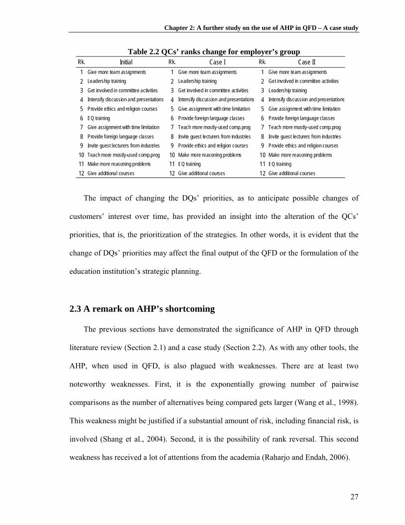
Chapter 2: A further study on the use of AHP in QFD – A case study
Table 2.2 QCs’ ranks change for employer’s group Rk. Initial Rk. Case I Rk. Case II
1 Give more team assignments 1 Give more team assignments 1 Give more team assignments
2 Leadership training 2 Leadership training 2 Get involved in committee activities
3 Get involved in committee activities 3 Get involved in committee activities 3 Leadership training
4 Intensify discussion and presentations 4 Intensify discussion and presentations 4 Intensify discussion and presentations
5 Provide ethics and religion courses 5 Give assignment with time limitation 5 Give assignment with time limitatio
6 EQ training 6 Provide foreign language classes 6 Provide foreign language classes7 Give assignment with time limitation 7 Teach more mostly-used comp.prog 7 Teach more mostly-used comp.prog
8 Provide foreign language classes 8 Invite guest lecturers from industries 8 Invite guest lecturers from industries9 Invite guest lecturers from industries 9 Provide ethics and religion courses 9 Provide ethics and religion courses
10 Teach more mostly-used comp.prog 10 Make more reasoning problems 10 Make more reasoning problems11 Make more reasoning problems 11 EQ training 11 EQ training
12 Give additional courses 12 Give additional courses 12 Give additional courses
n
The impact of changing the DQs’ priorities, as to anticipate possible changes of
customers’ interest over time, has provided an insight into the alteration of the QCs’
priorities, that is, the prioritization of the strategies. In other words, it is evident that the
change of DQs’ priorities may affect the final output of the QFD or the formulation of the
education institution’s strategic planning.
2.3 A remark on AHP’s shortcoming
The previous sections have demonstrated the significance of AHP in QFD through
literature review (Section 2.1) and a case study (Section 2.2). As with any other tools, the
AHP, when used in QFD, is also plagued with weaknesses. There are at least two
noteworthy weaknesses. First, it is the exponentially growing number of pairwise
comparisons as the number of alternatives being compared gets larger (Wang et al., 1998).
This weakness might be justified if a substantial amount of risk, including financial risk, is
involved (Shang et al., 2004). Second, it is the possibility of rank reversal. This second
weakness has received a lot of attentions from the academia (Raharjo and Endah, 2006).
27
Chapter 2: A further study on the use of AHP in QFD – A case study
Through a series of computer experiments and simulations, the author found that the
probability of rank reversal may get higher as the number of alternative and/or the
inconsistency of the decision gets larger. The detailed research methodology used in the
experiments can be found in Raharjo and Endah (2006). This finding is relevant to this
thesis since the use of AHP in QFD often involves a lot of alternatives, which is usually
reflected by the relatively large house of quality. This means that the chance of a rank
reversal to occur is indeed very high, especially when there is an alternative added or
deleted. Such case has, unfortunately, not been fully explored in this thesis and might be
an interesting study in the future.
2.4 Conclusion and implication
The aim of this chapter was to answer the question “In what ways does AHP,
considering its strength and weakness, contribute to an improved QFD analysis?” Based
on the literature, five reasons on the AHP’s contribution towards an improved QFD
analysis are identified. To further substantiate the contribution of AHP in QFD, a real-
world case study demonstrating the usefulness of AHP in QFD for improving higher
education quality of an engineering department has been provided. The case study also
empirically supports the five reasons since all of them were experienced while conducting
the study. Additionally, a remark on AHP’s shortcoming, when the number of alternatives
being compared gets larger, is also provided.
Some points to highlight in improving the use of the QFD in higher education, which
have been discussed in this study, are:
28

Chapter 2: A further study on the use of AHP in QFD – A case study
• It is important to use a relative measurement rather than a set of absolute values for
representing the importance rating values of DQs in QFD, and the AHP can be
considered as a beneficial tool to serve this purpose.
• A considerable attention should be paid to obtain a group preference. Using a
geometric mean would generally be better compared to using arithmetic mean in the
case where the group acts synergistically towards a common goal. A further treatment
on this issue can be found in Chapter 3 (Section 3.4.5).
• A careful check should be conducted to identify the true relationship between the DQs
and QCs in order to give a useful result. The QFD can be tailored to suit the particular
need of the users, for example, in determining how many house of quality to use. In
addition, for each customer, this study suggests that there should be one corresponding
QFD analysis.
For the case study, it can be concluded that endeavors that the higher education
institution should take as a main priority were to develop overall facility, reevaluate
existing curriculum, reduce unnecessary bureaucracy, improve lecturers’ qualification, and
provide more leadership/team training. Furthermore, in order to design effective and
efficient strategies, other subsequent/downstream analysis can be added, such as the gap
analysis, Strengths-Weaknesses-Opportunity-Threat (SWOT) analysis, optimization, and
so forth. An example of a downstream analysis, that is, to further use the relative QCs’
priorities which are in ratio scale as a basis for decision making, will be explained in
Chapter 8.
29

Chapter 2: A further study on the use of AHP in QFD – A case study
30
Alternative solutions (QCs) that are generated from the HoQ depend fully on level of
importance of the customer requirements (DQs). As shown in the sensitivity analysis,
changes in the DQs’ priorities may alter the priority order of the QCs; it may therefore
affect the education institution’s strategic planning. Such analysis is useful in the sense
that it may enable the education institution to be alert, proactive, and forward thinking
towards the dynamics of customer’s needs.
Referring back to the research problem (Section 1.1), it may now be rather clear that
unless the change of DQs’ priorities over time, that is, during product or service creation
process, is systematically anticipated, it is quite likely that the QFD team may end up with
misleading strategies if they rely on the past voice of the customer, that is, the priorities
collected at the start of the QFD’s use. In other words, it may be concluded that there is a
need to anticipate the change of customer’s needs, in terms of their weights, over time as
to provide a better strategic planning for the institution. In the next section, a further use of
AHP in QFD will be proposed via a generalized model.

Chapter 3: A further study on the use of AHP in QFD – A generalized model
CHAPTER 3
A FURTHER STUDY ON THE USE OF AHP IN QFD (PART 2 OF 2) –
A GENERALIZED MODEL
The purpose of this chapter is to provide the second part of a possible answer to the
research question “In what ways does AHP, considering its strength and weakness,
contribute to an improved QFD analysis?” Chapter 2 has described the first part of the
answer. To further show the AHP’s contribution in QFD, a generalized model is proposed.
The objective is to provide a more generic framework for QFD users to systematically
analyze and accurately quantify the subjective judgment, experience, and knowledge of
the design team. The advantage of the model is two-fold. First, it provides an alternative
way to construct the HoQ since all the elements are represented in the model. Second, it
provides more flexibility to take other relevant factors, such as the new product
development risk, into account when deriving the QCs’ priorities. This chapter is
reproduced from “Dealing with Subjectivity in Early Product Design Phase: A Systematic
Approach to Exploit QFD Potentials”, by Raharjo H, Brombacher AC, Xie M. 2008.
Published in Computers and Industrial Engineering.
3.1 Introduction
Since the focus of the QFD is on the early phase of products or services design process,
most of the input parameters are therefore highly subjective in nature (Xie et al., 2003;
Kim et al., 2007). Based on the survey results over 400 companies in the U.S. and Japan,
Cristiano et al. (2000) showed that the QFD analysis may only require a simple and
practical decision aid based upon the experience and judgment of the team. This is mainly
31

Chapter 3: A further study on the use of AHP in QFD – A generalized model
attributed to the fact that the QFD was born out of an industry need for ensuring design
quality. Hence, the accuracy level of these subjective experience and judgment will
significantly determine the quality of the QFD results.
In view of this, a method or approach that is capable to systematically analyze and
accurately quantify those subjective experience and judgments of the QFD team is highly
required. In the literature, the Analytic Hierarchy Process (Saaty, 1983, 1994), of which
generalized form is called the Analytic Network Process (Saaty, 1996), is known as one of
the most powerful management science tools to serve this purpose. The AHP/ANP has
been widely accepted as a realistic, flexible, simple, and yet mathematically rigorous
modeling technique in multiple criteria decision making field (Saaty, 1986; Liberatore,
1987; Sarkis and Sundarraj, 2006; Vaidya and Kumar, 2006). The AHP/ANP framework
can be considered as a powerful and necessary tool for making any strategic decision since
it is capable of taking into consideration multiple dimensions of information from multi-
party, either qualitative or quantitative, into the analysis (Dyer and Forman, 1992; Meade
and Sarkis, 1998; Meade and Presley, 2002).
In using the AHP in new product development field, Calantone et al. (1999) wrote that
“the AHP helps managers make more rational decisions by structuring the decision as
they see it and then fully considering all of the information”. In other words, the
AHP/ANP effectively facilitates managers in quantifying their subjective judgments,
experience, and knowledge of the complex system in an intuitive and natural way
(Mustafa and Al-Bahar, 1991; Dey, 2004) by systematically taking into account all the
relevant factors and their relative effects as well as interactions simultaneously.
As discussed in Chapter 2, the AHP has been used to derive DQs’ priorities in QFD
(Armacost et al., 1994; Lu et al., 1994; Park and Kim, 1998; Köksal and Eğitman, 1998;
32

Chapter 3: A further study on the use of AHP in QFD – A generalized model
Zakarian and Kusiak, 1999; Kwong and Bai, 2003; Raharjo et al., 2007; Li et al., 2009).
More recently, the use of the generalized form of AHP, namely, the ANP has been
growing considerably due to its very exceptional strength in addressing the inner-
relationship and interrelationship among the HoQ’s components (see Karsak et al., 2002;
Büyüközkan et al., 2004; Ertay et al., 2005; Kahraman et al., 2006; Partovi, 2006, 2007;
Pal et al., 2007).
The use of ANP in QFD, in general, can be categorized into two types. The first type,
of which model has been used by quite many researchers (Karsak et al., 2002;
Büyüközkan et al., 2004; Ertay et al., 2005; Kahraman et al., 2006; Pal et al., 2007), is
mainly based on the network model described in Saaty and Takizawa (1986). Compared to
the recent development of the ANP method, it might be considered as rather preliminary
(see Section 3.2.2). While the second type, which can be considered as a better
advancement of the use of ANP in QFD, employs the network model proposed recently by
Partovi (Partovi, 2006, 2007). However, the model is still rather restricted in the sense that
it uses ANP in addressing only two elements of HoQ, namely, the relationship matrix and
the correlation matrix (the roof of HoQ).
To fill in the niche of using ANP in QFD more effectively, a generic network model,
which serves as a generalized model from the previous research work, is proposed in this
chapter. Specifically, it takes into account the product design risk, competitors’
benchmarking information, and feedback information among the factors involved. It is
hoped that by using the proposed network model, the accuracy of the QFD results can be
further enhanced. In other words, by providing an effective way of quantifying and
analyzing QFD team’s subjective experience, knowledge, and judgments systematically,
33

Chapter 3: A further study on the use of AHP in QFD – A generalized model
the proposed model enables QFD practitioners to exploit more potentials of QFD as a
useful early product or service design tool.
In the next section (Section 3.2), a brief review of the AHP/ANP and its use in QFD
will first be provided. Section 3.3 describes the significance of some factors that are
selected to be included in the proposed network model. Then, the proposed network model,
which is the key contribution, is elaborated in Section 3.4. To give some practical insights
when using the proposed network model, an illustrative example was developed (Section
3.5). The illustrative example is provided to show how the proposed ANP model works in
practice. It is important to note that this is neither a full case study of ANP-QFD
application that results in a real product nor a part of a company’s work. The main
purpose here is rather to show how the model may work within realistic setting. Finally, a
discussion of the proposed method as well as possible future work will be described in
Section 3.6.
3.2 The ANP and its use in QFD
3.2.1 The ANP and the AHP
In dealing with large-scale strategic decisions with a high level of complexity, the
AHP has been accepted as one of the most important tools to systematically quantify the
subjective judgment of the decision makers (Zahedi, 1986; Bard and Sousk, 1990;
Rajasekera, 1990; Melachrinoudis and Rice, 1991; Mustafa and Al-Bahar, 1991; Suh et al.,
1994; Goh et al., 1998; Greiner et al., 2003; Dey, 2004; Wang et al., 2005; Vaidya and
Kumar, 2006). The generalization of the AHP, which is the ANP (Saaty, 1996), has
received an increasingly high attention recently (Meade and Sarkis, 1998; Meade and
34

Chapter 3: A further study on the use of AHP in QFD – A generalized model
Presley, 2002; Karsak et al., 2002; Shang et al., 2004; Kahraman et al., 2006; Sarkis and
Sundarraj, 2006).
The difference between AHP and ANP, in general, can be summarized in Table 3.1.
According to Shang et al. (2004), the ANP model, from a practical point of view, provides
practitioners with a generic model capable of being modified or enhanced, and yet
accountable, while from a research point of view, it gives researchers a novel
methodology for tackling strategic, tactical or operational decisions.
Table 3.1 Difference between AHP and ANP
Aspect AHP ANP
Structure Unidirectional Multidirectional
Type of relation Hierarchical Network
Nature of relationship Linear Non-linear
Nature of problem Simple Complex
Environment Static Dynamic
Feedback No Yes
3.2.2 Existing ANP’s use in QFD and its limitations
Recently, the trend of ANP increased use in QFD, as to overcome the limitation in the
use of AHP, has been remarkable. Some examples of the ANP’s use in QFD can be found
in Karsak et al. (2002), Büyüközkan et al. (2004), Ertay et al. (2005), Kahraman et al.,
(2006), Partovi (2006, 2007), and Pal et al. (2007). As mentioned previously, throughout
all the use of ANP in QFD, they can be categorized into two types.
The first type, of which examples can be found in Karsak et al. (2002), Büyüközkan et
al. (2004), Ertay et al. (2005), Kahraman et al. (2006), and Pal et al. (2007), basically
employs the network model described in Saaty and Takizawa (1986). However, compared
35

Chapter 3: A further study on the use of AHP in QFD – A generalized model
to the recent development of the ANP method, it is rather preliminary. There are two
limitations worth highlighting for this network model. First, it is the fact that it only
considers two clusters, which implies that the QFD team may only study the
interrelationship or inner-relationship among DQs and QCs irrespective of other relevant
important factors in the QFD itself, such as the competitive benchmarking information.
Moreover, there is no consideration of feedback information, which is one important
characteristic that clearly distinguishes ANP from AHP. In other words, the model
proposed is rather of restrictive form. Second, it is the computation which uses simple
matrix multiplications rather than the limit supermatrix approach (Saaty, 1996; Saaty and
Vargas, 1998). This implies that the approach may not be generalized easily.
The second type rests on the analytical model that was developed by Partovi (2006,
2007). It is argued that this framework adds quantitative precision to an otherwise ad hoc
decision making process. However, the use of the ANP in Partovi (2006, 2007) is still
rather limited, in the sense that it only addresses the relationship matrix and the correlation
matrix (the roof of HoQ). Furthermore, the use of the market segments as the first input in
the network model might make this approach rather difficult to be generalized since not all
QFD study may have such input. On the other hand, a fuller use of the ANP to deal with
the subjectivity inherent in the other elements of HoQ, such as the DQs or the competitive
benchmarking information, might further enhance the accuracy of the QFD results.
In view of these facts, this chapter proposes a more effective use of ANP in QFD
using a generic framework that is versatile enough to be customized for a particular firm.
Apart from taking into account the feedback information, it also considers the
competitors’ benchmarking information for the DQs and QCs as well as the new product
development risk. The proposed network model may also be regarded as a generalized
36

Chapter 3: A further study on the use of AHP in QFD – A generalized model
network model for the existing ANP model in QFD. It is hoped that the proposed network
model, by employing a systematic and effective approach for eliciting the team’s
judgments, may give more accurate information of the inner-relationship or
interrelationship among the factors that may be crucial to the QFD team’s success.
3.3 Some important factors in product design using QFD
This section provides some background of the three important factors that are
suggested to be used in the proposed network model in Section 3.4, those are, the new
product development risk, the benchmarking information, and the feedback information
consideration.
3.3.1 New product development (NPD) risk
The success of product innovation or new product development is necessarily related
to the ability of a firm to identify and manage the prevalent risks at the early stage of
product development (Keizer et al., 2002, 2005). Generally, risks are by nature subjective
and usually managed through a team effort, therefore the AHP/ANP can be regarded as
one of the most appropriate approaches to quantify, predict, analyze, and develop
strategies to better manage them (Dey, 2004). With regard to a risk management problem,
Mustafa and Al-Bahar (1991) wrote that the AHP is useful in documenting,
communicating an explicit, common, and shared understanding of risk, and thus become a
living picture of the management’s understanding of the risk involved.
Based on the work of Keizer et al. (2005) in providing an integral perspective on NPD
risk for supporting the success of breakthrough innovation projects, three risk categories,
37

Chapter 3: A further study on the use of AHP in QFD – A generalized model
within the ten most frequently perceived risk issues in the study, are suggested for
inclusion in the proposed network model. The three risk categories are ‘the consumer
acceptance and marketing risk’, ‘the supply chain risk’, and ‘the technology risk’. Each of
these risk categories comprises of many other types of risk, which will be described in the
next subsections. Note that these suggested risks are neither complete nor exhaustive.
Other relevant risk suitable to a particular firm or design process can be added accordingly
using the risk reference framework (RRF) proposed in Keizer et al. (2005).
A. Consumer Acceptance and Marketing Risk
This category may include the risk of consumers’ conviction that they get value for
money, product’s appeal to generally accepted values, product easy-in-use advantages, fit
of new product with consumer habits and/or user conditions, product offering additional
enjoyment, and so forth. For the sake of simplicity in using the generic network model,
this consumer acceptance and marketing risk may be associated with one or more detailed
risk elements mentioned above. Note that, in the study reported by Keizer et al. (2005),
this type of risk ranked in the first place as the most frequently perceived risk issue.
More importantly, it is worth highlighting that most of the elements in this category
are closely related with users’ or consumers’ expectation problem. In fact, this type of
problem has increasingly become a major source of customer complaints in the recent
decades, especially in the consumer electronics industry. Brombacher et al. (2005) showed
that the percentage of ‘No Fault Found’ has been significantly rising over the last two
decades. Such complaint (No Fault Found) refers to the situation where the product still
meets the technical specification, but is rejected because it does not satisfy the customer’s
expectation (see Den Ouden et al., 2006; Lu et al., 2007). This situation gives rise to a
38

Chapter 3: A further study on the use of AHP in QFD – A generalized model
newly developed class of product’s quality and reliability problem, namely, the ‘soft
reliability problem’ (Den Ouden, 2006; Brombacher et al., 2005)
B. Supply Chain Risk
Nowadays, it is virtually impossible for a company to work independently without
relying on other companies. In other words, a company has to be able to work
interdependently with a network of companies. Minderhoud and Fraser (2005) wrote that
it is increasingly common for products to be created by a globally distributed chain
involving multiple locations and companies. In other words, the product development
processes are getting more globally dispersed. This situation gives rise to more exposure
to risk, particularly in the supply chain. Therefore, there is an evident need to proactively
manage supply chain risk (Chopra and Sodhi, 2004; Finch, 2004; Tang, 2006). This
category may include the risk of constant and predictable product quality, capacity to meet
peak demands, reliability of each supplier in delivering according to requirements, long
term supply performance, suppliers’ readiness to accept modifications, and so forth. With
regard to using the proposed network model, this supply chain risk can be associated with
a more specific element that is relevant, as explained previously.
C. Technology Risk
This risk category may include the product and manufacturing technology risk, for
example, the fulfillment of the new products’ intended function, the interaction of product
in-use with sustaining materials, the components’ properties and functions, production’s
equipment and tools, the production system requirement, and so forth. Including the
technology risk in the proposed network model may help QFD team translate
39

Chapter 3: A further study on the use of AHP in QFD – A generalized model
technological advancements into products/services that meet customer needs, which is one
of the three levels of uncertainty that characterizes companies operating in rapidly
changing markets (Mullins and Sutherland, 1998). Furthermore, in dealing with the
complex task of prioritizing technology which involves many subjective criteria and
uncertainty, the AHP/ANP has been proven to be effective and practical (Melachrinoudis
and Rice, 1991; Suh et al., 1994). In using the proposed network model, this technology
risk may likewise be associated to one or more detailed elements described in the risk
reference framework (Keizer et al., 2005).
3.3.2 Benchmarking information
A benchmarking process provides insights necessary to effectively pinpoint the critical
success factors that set the most successful firms apart from their competitors, or to a
greater extent, that separates the winners from the losers (Cooper and Kleinschmidt, 1987,
1995). Korpela and Tuominen (1996) developed an AHP-based decision support system
for a continuous logistics benchmarking process to support logistics strategic management.
In view of the fact that a benchmarking process is a team effort, they further concluded
that the AHP is an effective tool for conducting group sessions in an analytical and
systematic manner.
In general, the QFD utilizes benchmarking information in two parts, namely, the
customer satisfaction benchmarking and the technical performance benchmarking.
According to the benchmarking types classification point of view (Zairi, 1992; Madu and
Kuei, 1993; or Camp, 1995), this chapter will only deal with the competitive or external
benchmarking, that is to deal with the ‘best-in-class’ competitors in the industry.
40

Chapter 3: A further study on the use of AHP in QFD – A generalized model
3.3.3 Feedback information
A feedback arc in the network model uniquely supplies useful information of the
cluster interrelationship, which is not possible in the case of a hierarchy. For example, in
the case of the proposed network model, the feedback arc from the QCs to the DQs
provides essential information to evaluate the DQs with respect to the QCs, as to
complement the counterpart relationship, that is, the relative importance of the QCs with
respect to the DQs.
A very simple example to signify the necessity of a feedback arc can be found in Saaty
(1996), which is known as the two-bridge problem, “Two bridges, both strong, but the
stronger is also uglier, would lead one to choose the strong but ugly one unless the criteria
themselves are evaluated in terms of the bridges, and strength receives a smaller value and
appearance a larger value because both bridges are strong”. In brief, without considering
the feedback arc, one may not be able to capture a complete interrelationship of the
clusters. In other words, the results’ accuracy of the analysis may be doubtful.
3.4 The proposed generalized model
The proposed model, which is based on the ANP, gives a more generic framework for
QFD users to systematically analyze and accurately quantify the subjective judgment,
experience, and knowledge of the design team. The network model, while taking into
account several important factors in new product design phase, such as new product
development risk, benchmarking information, and feedback information simultaneously,
enables a fuller use of QFD as a customer-driven tool.
41

Chapter 3: A further study on the use of AHP in QFD – A generalized model
In the next subsections, the proposed network model will first be described, and
followed with the elaboration of its correspondence to the elements in the HoQ. Then, a
step-by-step procedure to use the proposed network model, which is based on the HOQ’s
elements, is suggested. The types of questions that are used to elicit the QFD team’s
judgments will be explained subsequently. Finally, some considerations of the group
decision making process and the use of fuzzy theory along with the proposed model are
discussed.
3.4.1 The model
The proposed network model is shown in Figure 3.1. It consists of five clusters, that is,
the Goal, which is to achieve best product design, the demanded quality (DQ), the quality
characteristic (QC), the new product development risk (NPD Risk), and the competitors’
benchmarking information. Each cluster comprises of several nodes, for example, the DQ
cluster has m nodes. The arcs used in the network model can be categorized into three
main types, namely, the outer dependence arc, the inner-dependence arc, and the feedback
arcs.
42

Chapter 3: A further study on the use of AHP in QFD – A generalized model
Figure 3.1 The proposed ANP framework for QFD
The outer dependence arcs, which are denoted in arcs number 1, 3, 6, 8, 10, 12, 14, 16
(solid lines) of Figure 3.1, show a dependence condition between the controlling and
controlled cluster. A controlling cluster (source) is the cluster from which the arc
emanates, while a controlled cluster (sink) is the cluster which the arc points to. The inner-
dependence arcs (a loop), which are denoted in arcs number 2, 4, 7, 13 (dotted lines),
show a dependence condition among the elements within a cluster. The feedback arc looks
similar to the outer dependence arc, but with a reverse direction. In the network model
above, it is shown in arc number 5, 9, 11, 15, 17 (dashed lines).
3.4.2 The model and the HoQ’s components
It is interesting to see that all of the components in the HoQ, which is the main part of
the QFD methodology, can be represented by the most of the arcs described in Figure 3.1.
Specifically, the demanded quality (DQ) part or voice of the customer (VOC), which is
the most critical determinant of the QFD success (Cristiano et al., 2001), is represented in
43

Chapter 3: A further study on the use of AHP in QFD – A generalized model
arcs 1, 2, 5, 8, and 14. The quality characteristics (QC) part corresponds to arcs 3, 4, 10,
and 16. The relationship matrix, which is in the center part of the HoQ, is represented in
arcs 3 and arc 5. The DQ’s competitive benchmarking information is represented in arc 15,
while the QC’s competitive benchmarking information is represented in arc 17. Note that
arc 14 and arc 16, respectively, corresponds to the competitive target setting stage for the
DQ and the QC. Finally, the correlation matrix or the roof of the HoQ, which represents
the interrelationship among the QCs, is represented in arc 4.
In dealing with the roof of the HoQ, which is a vital and yet often ignored or
oversimplified part in the QFD (Kwong et al., 2007), the proposed network model
provides a more effective way in handling the roof matrix correlation values. Unlike the
traditional QFD, it offers a more flexible approach in accounting for the inner-relationship
among the QCs. More specifically, it eliminates the need to carry out a post-analysis
evaluation of the roof matrix correlations values for adjusting the QCs priorities, and at
the same time, relaxes the symmetrical assumption of the relationship between the QCs
(Partovi, 2006, 2007).
To sum up, it can be said that the proposed network model has addressed all of the
most important components in the HoQ. Thus, it provides a better way to exploit the QFD
potentials. In other words, by using the proposed network model, QFD users are able to
accurately fill in the values of all elements in the HOQ in a more systematic manner.
Hence, the accuracy of the result may be significantly improved, particularly with the
incorporation of some other important information which is beyond the basic QFD
framework, such as the interrelationship among the DQs and the consideration of the NPD
risk with respect to a constantly changing environment.
44

Chapter 3: A further study on the use of AHP in QFD – A generalized model
3.4.3 A suggested step-by-step procedure for using the model
After constructing the network model of the design problem, the next step is to elicit
the QFD team’s judgments. The judgment elicitation process is carried out using the
ANP/AHP’s pairwise comparison question (Saaty, 1983, 1986). The detailed question for
each arc will be explained in the next subsection (Section 3.4.4). It is worth highlighting
that in each pairwise comparison matrix, the aggregated preference of the QFD team can
be obtained either using a consensus vote or geometric mean (see Section 3.4.5). After
taking the aggregated preference, the relative importance weight of the pairwise
comparison matrices can be computed using the eigenvector method (Saaty, 1994). The
Super Decision software may be used for this purpose. It can also be used to do an
inconsistency check of the judgments. If the inconsistency level goes beyond a threshold
value, for example, 10%, then a resurvey or another round of judgment elicitation process
can be conducted (Saaty, 1994, 1996).
To make the judgment elicitation process more efficient, a step-by-step procedure of
using the proposed network model, which is based on the sequence that is used in the
QFD method, is suggested as follows. Note that, for all the arcs, in the case of no
relationship, a blank can be added accordingly (Partovi, 2006, 2007).
A. General network framework
Step 1. Adopt the generic (proposed) model, modify if necessary.
B. Listening to the customer
Step 2. Add necessary nodes within each cluster. For the DQ cluster, the nodes are
obtained based on customer’s survey data. Note that the guidance of the QFD
team in helping the customers express their ‘voices’ or judgments is essential in
this VOC collection phase. For the QC cluster, the NPD risk cluster, and the
45

Chapter 3: A further study on the use of AHP in QFD – A generalized model
Competitors cluster, the nodes can be obtained based on the judgment,
experience, and knowledge of the team.
Step 3. Elicit the QFD team’s judgment using the pairwise comparison for arc 1 and arc
2. Arc 1 is used to obtain the priorities of the DQs, while arc 2 is used to obtain
the inner relationship among the DQs.
C. The relationship matrix
Step 4. Elicit the QFD team’s judgment using the pairwise comparison for arc 3 and arc
5. These two arcs show the bidirectional relationship between the DQs and the
QCs.
D. The HOQ roof
Step 5. Elicit the QFD team’s judgment using the pairwise comparison for arc 4. As
mentioned previously, this eliminates the need to carry out a post-analysis
evaluation of the roof matrix correlations values (Partovi, 2006, 2007).
E. The competitors' general information
Step 6. Elicit the QFD team’s judgment using the pairwise comparison for arc 12 and arc
13. Arc 12 is used to obtain general information on how strong one competitor is
compared to the others, while arc 13 is used to obtain information on the inner
relationship among the competitors themselves.
F. The competitor performance evaluation
Step 7. Elicit the QFD team’s judgment using the pairwise comparison for arc 15 and arc
17. Arc 15 is used to evaluate the competitors’ performance with respect to the
DQs, while arc 17 is used to evaluate their performance with respect to the QCs.
46

Chapter 3: A further study on the use of AHP in QFD – A generalized model
G. The NPD risk information
Step 8. Elicit the QFD team’s judgment using the pairwise comparison for arc 6 to arc 11.
Note that this additional information is beyond the basic HOQ, it is included here
for improving the QFD results’ accuracy, considering the market dynamics.
H. The competitive target setting for DQs
Step 9. Elicit the QFD team’s judgment using the pairwise comparison for arc 14. When
eliciting the judgments for arc 14, the design team might consider three previous
factors, those are, the priorities of the DQs (arc 1), the general information of the
competitors (arc 12), and the competitors performance with respect to the DQs
(arc 15).
I. Obtaining QCs’ priorities for technical target setting
Step 10. Elicit the QFD team’s judgment for the clusters to obtain a cluster matrix using
the pairwise comparison.
Step 11. Construct the unweighted supermatrix using the derived priorities. Afterwards,
construct the weighted supermatrix by multiplying the unweighted supermatrix
by the cluster matrix.
Step 12. Compute the limit supermatrix by raising the weighted supermatrix to the power
of 2k+1, where k is an arbitrarily large number to allow convergence. The
supermatrix concept is parallel to the Markov chain process (Saaty, 1983).
Step 13. Normalize the converged or stable priorities.
J. The competitive target setting for QCs
Step 14. Elicit the QFD team’s judgment using the pairwise comparison for arc 16. It is
suggested that when eliciting the judgment for this arc, the QFD team may
consider the QCs priorities obtained from Step 13, the general information of the
47

Chapter 3: A further study on the use of AHP in QFD – A generalized model
competitors (arc 12), and the competitors’ performance with respect to the QCs
(arc 17). Note that this is in line with the standard QFD methodology, where the
competitive target setting or the competitive technical assessment (Chan and Wu,
2002b) for the QCs is done after knowing the priorities of the QCs.
K. The final priorities
Step 15. After filling the information for arc 16, repeat Step 11 to Step 13, and obtain the
final priorities for all clusters. Other further analysis can be employed
subsequently, such as optimization.
3.4.4 Types of questions to elicit decision makers’ judgments
Based on the relationships that are established in the network model, this subsection
describes the type of pairwise comparison questions that are used to elicit the relative
importance between and within the five corresponding clusters. According to the arc’s
number in Figure 3.1, Table 2.2 shows the questions that can be used to elicit the QFD
team’s judgments. Note that the questions may be phrased differently, but with the same
meaning, to suit a particular condition.
Table 3.2 Questions for eliciting QFD team’s judgments
Arc Question
1 With respect to achieving best design, how important is DQ1 compared to DQ2?
2 With respect to controlling DQ1, how important is DQ2 compared to DQ3?
3 With respect to satisfying DQ1, how important is QC1 compared to QC2?
4 With respect to controlling QC1, how important is QC2 compared to QC3?
5 With respect to QC1, how important is DQ1 compared to DQ2?
6 With respect to achieve best design, how sensitive is Risk1 compared to Risk2?
7 With respect to controlling Risk1, how important is Risk2 compared to Risk3?
48
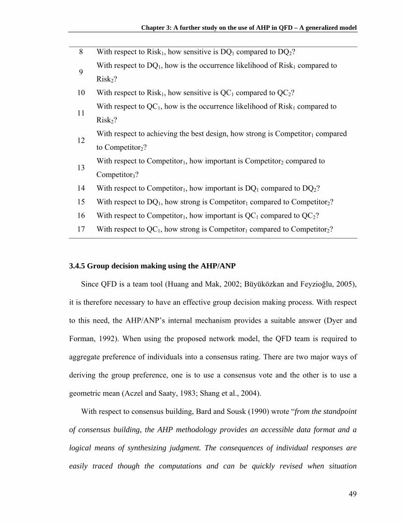
Chapter 3: A further study on the use of AHP in QFD – A generalized model
8 With respect to Risk1, how sensitive is DQ1 compared to DQ2?
9 With respect to DQ1, how is the occurrence likelihood of Risk1 compared to
Risk2?
10 With respect to Risk1, how sensitive is QC1 compared to QC2?
11 With respect to QC1, how is the occurrence likelihood of Risk1 compared to
Risk2?
12 With respect to achieving the best design, how strong is Competitor1 compared
to Competitor2?
13 With respect to Competitor1, how important is Competitor2 compared to
Competitor3?
14 With respect to Competitor1, how important is DQ1 compared to DQ2?
15 With respect to DQ1, how strong is Competitor1 compared to Competitor2?
16 With respect to Competitor1, how important is QC1 compared to QC2?
17 With respect to QC1, how strong is Competitor1 compared to Competitor2?
3.4.5 Group decision making using the AHP/ANP
Since QFD is a team tool (Huang and Mak, 2002; Büyüközkan and Feyzioğlu, 2005),
it is therefore necessary to have an effective group decision making process. With respect
to this need, the AHP/ANP’s internal mechanism provides a suitable answer (Dyer and
Forman, 1992). When using the proposed network model, the QFD team is required to
aggregate preference of individuals into a consensus rating. There are two major ways of
deriving the group preference, one is to use a consensus vote and the other is to use a
geometric mean (Aczel and Saaty, 1983; Shang et al., 2004).
With respect to consensus building, Bard and Sousk (1990) wrote “from the standpoint
of consensus building, the AHP methodology provides an accessible data format and a
logical means of synthesizing judgment. The consequences of individual responses are
easily traced though the computations and can be quickly revised when situation
49

Chapter 3: A further study on the use of AHP in QFD – A generalized model
warrants”. However, the consensus vote approach might not be easy to use since it
requires an agreement of all the team’s members for each entry in the pairwise comparison
matrices.
Nevertheless, if it is assumed that the team is a collection of synergistic individuals
who act together towards a common goal, as in the case of the QFD team, rather than
separate individuals, then the geometric mean approach is the most suitable method
(Forman and Peniwati, 1998). Moreover, the geometric mean of the set of individual
judgments preserves the ratio scale and satisfies the reciprocal property to guarantee that
the eigenvector method still holds (Aczel and Saaty, 1983). The geometric mean approach,
which is suggested in using the proposed framework, can be expressed as follows:
nn
k
kij
Gij aa
1
1⎥⎦
⎤⎢⎣
⎡= ∏
=
(3.1)
where:
n = the number of decision makers
Gija = the group judgment of the (i,j) element in the reciprocal matrix
Note that the formula above assumes that the individuals are of equal importance;
otherwise, one may use the weighted geometric mean.
3.4.6 Fuzziness in the AHP/ANP
Another important thing to highlight is the incorporation of fuzziness in the judgment
of the QFD team when using the AHP/ANP model. The fuzzy theory is expected to help
the QFD team better quantify the subjectivity, particularly in terms of representing
linguistic expression (see Kwong and Bai, 2003; Kahraman et al., 2006). Nevertheless, by
50
Chapter 3: A further study on the use of AHP in QFD – A generalized model
its very nature, the internal mechanism of the AHP/ANP in eliciting judgment has taken
into account the fuzziness in decision maker’s judgment (Saaty, 2006; Saaty and Tran,
2007). Therefore, the applying fuzzy theory into the AHP context will be of little value
and further complicate the process. As noted by Saaty (2006), “Enforce judgments by an
outsider who likes fuzzy number crunching needs proof of the validity of its outcome, and
we have shown by examples the outcome is not only close to what the AHP obtains
without fuzziness but can also be worse, so it is unjustified to use fuzzy in the AHP.”
In sum, to deal with the subjectivity of judgments inherent in the QFD process, it is
suggested to use either the AHP/ANP approach or the fuzzy theory approach separately
since combining both approaches will further complicate the process and be of little
additional value. Some examples for using fuzzy theory separately from the AHP/ANP in
the QFD can be found in Khoo and Ho (1996), Kim et al. (2000), Karsak (2004), Chen et
al. (2004, 2006), or Fung et al. (2006). The issue of “which approach performs better in
dealing with the subjectivity of judgments in the QFD process” is beyond the scope of this
thesis and might be an interesting topic to be addressed in the future.
3.5 An illustrative example
This section provides an illustrative example that was developed by the author after
having intensive discussions with people who are knowledgeable in dealing with the
increasingly important soft reliability problem (see Section 3.3.1.A), especially for
consumer electronic products in European countries. Due to the soft reliability problem,
there are more and more products being returned to the company although they are not
defective (Brombacher et al., 2005; Den Ouden, 2006). One of the effective ways to tackle
51

Chapter 3: A further study on the use of AHP in QFD – A generalized model
this problem is to improve product’s “ease of use” (Sciarrotta, 2003), for example, by
designing a satisfactory out-of-box experience for the consumer.
It is quite natural that users, after purchasing a consumer electronic product, want to
get start to work productively as soon as possible (Fouts, 2000; Marcus, 2005). The first
impression the users may have on the products as well as the company may depend
largely on the out-of-box experience, which includes the experience in taking the product
out of the box (unpacking), setting up its hardware and software, and putting it into use
(Ketola, 2005; IBM, 2007).
For the sake of simplicity and to give readers some insights on how the proposed
network model may work in practice, this illustrative example will focus on one element
of the entire out-of-box experience of a PC media center, that is, the software setup and
configuration phase. The objective of this example is to design a software setup
experience that may satisfy users’ needs. The users’ needs or demanded qualities become
the first ingredient of the QFD process. Afterwards, the QFD team translates those DQs
into QCs. Lastly, considering the NPD risk, the benchmarking information, and the
feedback information, the QFD team systematically decide the importance of the quality
characteristics. The importance of the QCs, which is the final result, is reflected
quantitatively in terms of relative priorities. Those priorities can be dovetailed with the
other subsequent analysis, such as optimization with regard to the limited resources (see
Chapter 8).
Following closely the step-by-step procedure described in Section 3.4.3, the
implementation of the proposed network model for achieving a best software setup
experience may proceed as follows:
52
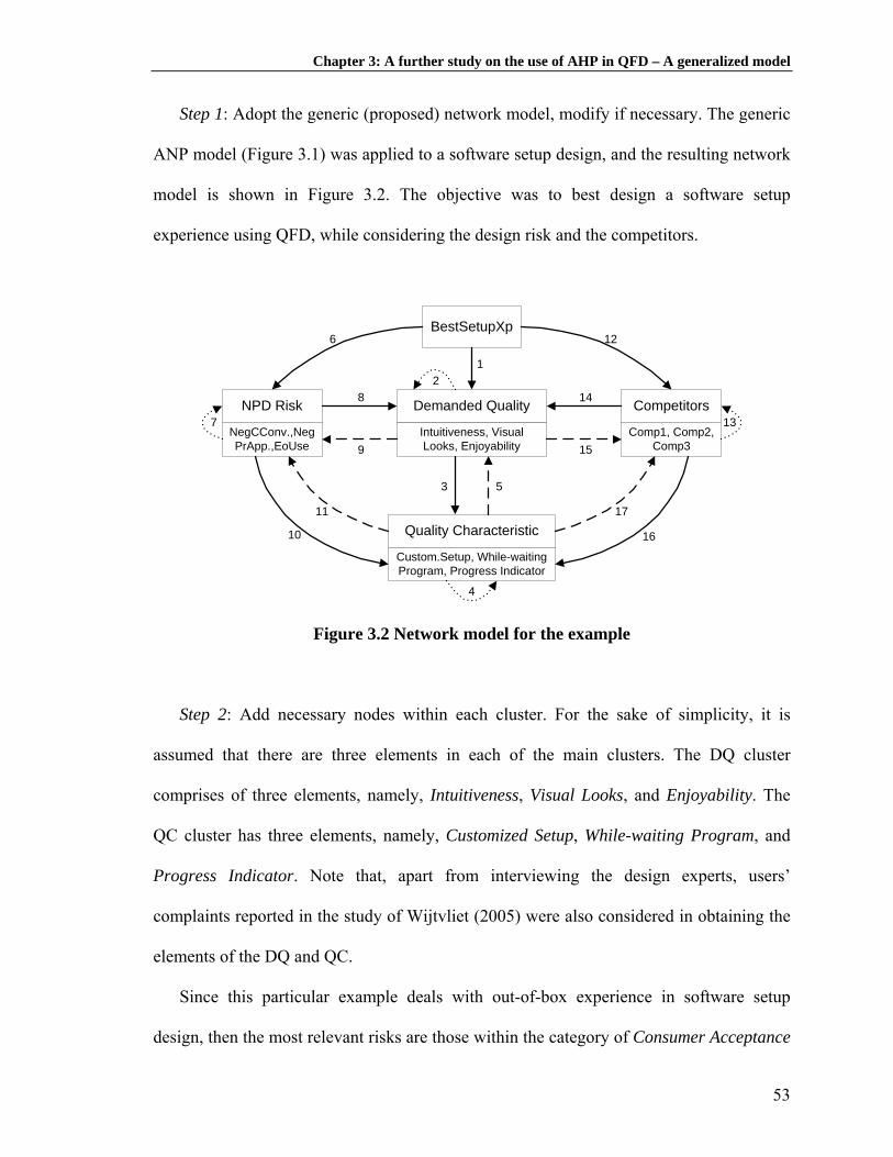
Chapter 3: A further study on the use of AHP in QFD – A generalized model
Step 1: Adopt the generic (proposed) network model, modify if necessary. The generic
ANP model (Figure 3.1) was applied to a software setup design, and the resulting network
model is shown in Figure 3.2. The objective was to best design a software setup
experience using QFD, while considering the design risk and the competitors.
BestSetupXp
NegCConv.,NegPrApp.,EoUse
NPD Risk
Comp1, Comp2, Comp3
CompetitorsDemanded Quality
Intuitiveness, Visual Looks, Enjoyability
Quality Characteristic
Custom.Setup, While-waiting Program, Progress Indicator
12
3
4
5
6
7
8
9
10
11
12
13
14
15
16
17
Figure 3.2 Network model for the example
Step 2: Add necessary nodes within each cluster. For the sake of simplicity, it is
assumed that there are three elements in each of the main clusters. The DQ cluster
comprises of three elements, namely, Intuitiveness, Visual Looks, and Enjoyability. The
QC cluster has three elements, namely, Customized Setup, While-waiting Program, and
Progress Indicator. Note that, apart from interviewing the design experts, users’
complaints reported in the study of Wijtvliet (2005) were also considered in obtaining the
elements of the DQ and QC.
Since this particular example deals with out-of-box experience in software setup
design, then the most relevant risks are those within the category of Consumer Acceptance
53

Chapter 3: A further study on the use of AHP in QFD – A generalized model
and Marketing risk (see Section 3.3.1). Hence, for the NPD Risk cluster, the three
elements, using the risk reference framework (Keizer et al., 2005), are Negative
Consumers’ Conviction, Negative Product’s Appeal, and Ease of Use Risk. Lastly, there
are three fictitious ‘best-in-class’ competitors that were selected for this study, those are,
the first competitor (Comp1), the second competitor (Comp2), and the third competitor
(Comp3).
In terms of the DQ, the focus area of Comp1, Comp2, and Comp3 are the Intuitiveness,
the Enjoyability, and the Visual Looks of the software setup process, respectively. In terms
of the QC, Comp1 focuses more on designing user-friendly Customized Setup, Comp2
focuses more on developing enjoyable While-waiting Program, while Comp3 has a
typically elegant Progress Indicator. Additionally, Comp1 and Comp2 have been
competing for each other, while Comp3 is a new player for producing the PC Media
Center. Super Decision software was used to construct the network model and obtain the
final priorities.
After constructing the network model of the PC design problem, the next step is to
elicit the QFD team’s judgments for each of the arcs accordingly. A sample of a pairwise
comparison questionnaire, along with some information for guiding the users and designer
to express their judgments and experience, can be found in Appendix A. The typical
pairwise comparison question for each arc (listed in Table 3.2) was used to elicit the QFD
team’s judgments.
With regard to the aggregated group preference, it is assumed that a consensus vote
was achieved. Otherwise, the geometric mean can be used (see Section 3.4.5). For each of
the pairwise comparison matrix, a maximum inconsistency value of 0.1 (Saaty, 1994) was
54

Chapter 3: A further study on the use of AHP in QFD – A generalized model
used to decide whether there is a need to do a resurvey. The priorities of each pairwise
comparison matrix were computed using the Super Decision software.
To make the judgment elicitation process more efficient, it was carried out according
to the HoQ’s elements, as described in Section 3.4.3. The judgments results, which are
grouped by the arc’ category, can be found in Appendix B.
Step 3: Elicit the QFD team’s judgment using the pairwise comparison for arc 1 and
arc 2. The result for arc 1 (Table B1), of which data were obtained from the customer,
shows that the customer regards the Intuitiveness of a software setup as the most important
thing (0.714). The question used for arc 2 might be like: “With respect to controlling
Visual Looks, how important is Intuitiveness compared to Enjoyability?”. Table B2 shows
that, with respect to controlling Visual Looks, the Intuitiveness has more influence than the
Enjoyability (by three times), which is intuitively justifiable.
Step 4: Elicit the QFD team’s judgment using the pairwise comparison for arc 3 and
arc 5. Arc 3 represents the QFD team’s judgment on how important the QCs are with
respect to satisfying the DQs, while arc 5 represents the feedback information to evaluate
the DQs with respect to the QCs. The question used for arc 3 can be like: “With respect to
satisfying Intuitiveness, how important is Customized Setup compared to While-waiting
Program?”, and as shown in Table B1, the Customized Setup is five times more important
than the While-waiting Program. The results for all pairwise comparisons done for arc 3
can be summarized as follows. The Customized Setup plays the most important role on
Intuitiveness (0.637), while the While-waiting Program on the Visual Looks (0.714) and
the Enjoyability (0.709).
The pairwise comparison question used for arc 5 can be like: “With respect to
Progress Indicator, how important is Enjoyability compared to Visual Looks?”. It is easy
55

Chapter 3: A further study on the use of AHP in QFD – A generalized model
to see that the Visual Looks of a progress indicator can be much more important than its
Enjoyability. On the other hand, for the Customized Setup, its Enjoyability appeared to be
the most important thing to be improved upon. This is reasonable because a Customized
Setup should basically be intuitive. For the While-waiting Program, its Intuitiveness
appeared to the most important attribute (see Table B3). Again, this is because it is
assumed that the basic function of a While-waiting Program is to make the waiting
process enjoyable. Note that this type of information has enabled the QFD team to take
into account the important feedback, which is not possible when using the AHP.
Unfortunately, it has been largely overlooked in the existing literature.
Step 5: Elicit the QFD team’s judgment using the pairwise comparison for arc 4. The
question posed can be like: “With respect to controlling While-waiting Program, how
important is Customized Setup compared to Progress Indicator?”. It is shown that all the
controlled QCs have the same importance level. After further investigation with the design
experts, such condition took place because the level of this information (granularity) is
very specific. Therefore, this information may only be reserved to the programmer of the
software. As for this example, they are assumed to be equally important.
Step 6: Elicit the QFD team’s judgment using the pairwise comparison for arc 12 and
arc 13. Arc 12 (Table B1) gives the priorities of the best-in-class competitors towards
achieving the best design of a software setup experience. The questions posed for this arc
can be like: “With respect to achieving best software setup experience, how strong is
Comp1 compared to Comp2?”. The result shows that Comp1 (0.500) appeared to be the
strongest competitor. Arc 13 shows the relationship among the competitors themselves.
As shown in Table B2, Comp1 and Comp2 are competing with each other. While Comp3,
as a new player, regards the two other competitors as equally important.
56

Chapter 3: A further study on the use of AHP in QFD – A generalized model
Step 7: Elicit the QFD team’s judgment using the pairwise comparison for arc 15 and
arc 17. These two arcs evaluate the strength of the competitors with respect to the DQs
and QCs. Readers may check that the results shown in Table B3 agree with the
competitors’ profile described previously. The question posed can be like: “With respect
to Intuitiveness, how strong is Comp1 compared to Comp2?”.
Step 8: Elicit the QFD team’s judgment using the pairwise comparison for arc 6 to arc
11. With respect to the risks involved, the question posed for arc 6 can be like “With
respect to the risk of software setup experience, how sensitive is Negative Consumer's
Conviction compared to Ease of Use Risk?”. Note that, for all priorities in this study, it is
assumed that the higher the values, the more important they become. Thus, in the case of
the risk involved, the emphasis is placed on those relatively riskier elements since they are
very critical in creating customers satisfaction/dissatisfaction. It can be seen from Table
B1 that the Ease of Use Risk is the most sensitive one, and thus it receives the highest
priority.
Arc 7 represents the inner relationship among the risks themselves. It is worth noting
that there are two ‘NA’ (Not Applicable) judgments in this cluster (Table B2). This is due
to the fact that the entities being compared lack a contextual meaning. For example, a
question like “With respect to controlling Negative Product’s Appeal, how important is
Negative Consumer’s Conviction compared to Ease of Use Risk?” is virtually impossible
to answer since there is no relationship among the entities.
For arc 8, the question posed can be like: “With respect to giving rise to Negative
Consumers’ Conviction, how sensitive is the Intuitiveness compared to the Visual Looks?”.
As shown in Table B1, the Intuitiveness is five times riskier or more sensitive than the
Visual Looks. From the results in arc 8, it can be said that the intuitiveness of software
57

Chapter 3: A further study on the use of AHP in QFD – A generalized model
setup process is the most sensitive item that will cause negative consumer’s conviction
and ease of use risk, while the visual looks appears to be the most sensitive in giving rise
to negative product’s appeal. With respect to all the risks (Arc 10 in Table B1), the
Customized Setup appeared to be the most sensitive QC. This is quite reasonable since the
customized setup is the first thing that the users encounter. Furthermore, the two other
QCs may, in general, also be controlled by the customized setup. A similar question as in
arc 8 can be used accordingly.
Arc 9 and arc 11 evaluate the occurrence likelihood of the risks with respect to the
DQs and QCs. The question posed can be like: “With respect to While-waiting Program,
how is the occurrence likelihood of Negative Consumers’ Conviction compared to Ease of
Use Risk?”. As shown in Table B3, the Ease of Use is the least important risk with respect
to the While-waiting Program. This is quite intuitive since a while-waiting program has no
explicit relationship with the ease of use part of a software setup. Other results can be
interpreted accordingly.
Step 9: Elicit the QFD team’s judgment using the pairwise comparison for arc 14. The
question posed can be like: “With respect to Comp1, how important is Intuitiveness
compared to Visual Looks?”. The result for this question (Table B1) shows that the
Intuitiveness is seven times more important (very strong) than the Visual Looks. It is easy
to see that such a high value was assigned due to the fact that the Intuitiveness is the most
important attribute from the customer’s perspective (see arc 1) and Comp1 performs very
well with respect to this attribute (see arc 15). Moreover, Comp1 is also the strongest
competitor (arc 12).
Step 10: Elicit the QFD team’s judgment for the clusters to obtain a Cluster Matrix
using the pairwise comparison. For the sake of simplicity, it is assumed that all the
58

Chapter 3: A further study on the use of AHP in QFD – A generalized model
clusters in the network model carry equal weight. The resulting cluster matrix is shown in
Table 3.3.
Table 3.3 Cluster matrix Cluster 1.GOAL 2.DQ 3.Risk 4.Competitors 5.QC1.GOAL 0.000 0.000 0.000 0.000 0.0002.DQ 0.333 0.500 0.333 0.333 0.5003.Risk 0.333 0.000 0.333 0.000 0.0004.Competitors 0.333 0.000 0.000 0.333 0.0005.QC 0.000 0.500 0.333 0.333 0.500
Step 11: Construct the unweighted supermatrix using the derived priorities. The
unweighted supermatrix is shown in Table 3.4. Note that this matrix constitutes all the
previously derived priorities. For example, with respect to the goal (objective), the priority
of each DQ element (see the third column of Table 3.4 under “Goal”), namely, the
Intuitiveness (0.714), the Visual Looks (0.143), and the Enjoyability (0.143), is exactly the
same as obtained in Table B1 (arc 1). Likewise, the remaining parts in Table 3.4 can be
interpreted accordingly.
Table 3.4 Unweighted supermatrix without arc 16
1.GOALB.SetupXp Intuitive Vlooks Enjoy. NegCCon NegPrAp EoURisk Comp1 Comp2 Comp3 CustSet Wh-wait ProInd
1.GOAL B.SetupXp 0.000 0.000 0.000 0.000 0.000 0.000 0.000 0.000 0.000 0.000 0.000 0.000 0.0002.DQ Intuitive 0.714 0.000 0.750 0.500 0.714 0.125 0.750 0.778 0.683 0.637 0.260 0.600 0.286
Vlooks 0.143 0.750 0.000 0.500 0.143 0.750 0.125 0.111 0.117 0.258 0.327 0.200 0.571Enjoy. 0.143 0.250 0.250 0.000 0.143 0.125 0.125 0.111 0.200 0.105 0.413 0.200 0.143
3.Risk NegCCon 0.143 0.208 0.238 0.550 0.000 0.000 0.000 0.000 0.000 0.000 0.167 0.595 0.300NegPrAp 0.143 0.131 0.625 0.240 0.250 0.000 0.000 0.000 0.000 0.000 0.167 0.276 0.600EoURisk 0.714 0.661 0.137 0.210 0.750 0.000 0.000 0.000 0.000 0.000 0.667 0.128 0.100
4.Competitors Comp1 0.500 0.750 0.113 0.167 0.000 0.000 0.000 0.000 0.750 0.500 0.750 0.200 0.106Comp2 0.250 0.125 0.179 0.667 0.000 0.000 0.000 0.750 0.000 0.500 0.125 0.683 0.193Comp3 0.250 0.125 0.709 0.167 0.000 0.000 0.000 0.250 0.250 0.000 0.125 0.117 0.701
5.QC CustSet 0.000 0.637 0.143 0.179 0.659 0.600 0.732 0.000 0.000 0.000 0.000 0.500 0.500Wh-wait 0.000 0.105 0.714 0.709 0.156 0.200 0.130 0.000 0.000 0.000 0.500 0.000 0.500ProInd 0.000 0.258 0.143 0.113 0.185 0.200 0.138 0.000 0.000 0.000 0.500 0.500 0.000
2.DQ 3.Risk 4.Competitors 5.QC
To derive the final weights of the proposed network model, a column stochastic
supermatrix is needed (Saaty, 1996). Therefore, the unweighted supermatrix is multiplied
by the cluster matrix to obtain the weighted supermatrix. The resulting weighted
supermatrix, which is column stochastic, is shown in Table 3.5.
59

Chapter 3: A further study on the use of AHP in QFD – A generalized model
Table 3.5 Weighted supermatrix without arc 16 1.GOAL
B.SetupXp Intuitive Vlooks Enjoy. NegCCon NegPrAp EoURisk Comp1 Comp2 Comp3 CustSet Wh-wait ProInd1.GOAL B.SetupXp 0.000 0.000 0.000 0.000 0.000 0.000 0.000 0.000 0.000 0.000 0.000 0.000 0.0002.DQ Intuitive 0.238 0.000 0.188 0.125 0.238 0.063 0.375 0.389 0.342 0.318 0.065 0.150 0.071
Vlooks 0.048 0.188 0.000 0.125 0.048 0.375 0.063 0.056 0.058 0.129 0.082 0.050 0.143Enjoy. 0.048 0.063 0.063 0.000 0.048 0.063 0.063 0.056 0.100 0.052 0.103 0.050 0.036
3.Risk NegCCon 0.048 0.052 0.060 0.137 0.000 0.000 0.000 0.000 0.000 0.000 0.042 0.149 0.075NegPrAp 0.048 0.033 0.156 0.060 0.083 0.000 0.000 0.000 0.000 0.000 0.042 0.069 0.150EoURisk 0.238 0.165 0.034 0.052 0.250 0.000 0.000 0.000 0.000 0.000 0.167 0.032 0.025
4.Competitors Comp1 0.167 0.188 0.028 0.042 0.000 0.000 0.000 0.000 0.375 0.250 0.188 0.050 0.027Comp2 0.083 0.031 0.045 0.167 0.000 0.000 0.000 0.375 0.000 0.250 0.031 0.171 0.048Comp3 0.083 0.031 0.177 0.042 0.000 0.000 0.000 0.125 0.125 0.000 0.031 0.029 0.175
5.QC CustSet 0.000 0.159 0.036 0.045 0.220 0.300 0.366 0.000 0.000 0.000 0.000 0.125 0.125Wh-wait 0.000 0.026 0.179 0.177 0.052 0.100 0.065 0.000 0.000 0.000 0.125 0.000 0.125ProInd 0.000 0.065 0.036 0.028 0.062 0.100 0.069 0.000 0.000 0.000 0.125 0.125 0.000
2.DQ 3.Risk 4.Competitors 5.QC
Step 12: Compute the limit supermatrix by raising the weighted supermatrix to the
power of 2k+1, where k is an arbitrarily large number to allow convergence. The long
term priorities or stable weighted values of the weighted supermatrix, which are reflected
in the limit supermatrix, are shown in Table 3.6. All the clusters appeared to converge.
Table 3.6 Limit supermatrix without arc 16
1.GOALB.SetupXp Intuitive Vlooks Enjoy. NegCCon NegPrAp EoURisk Comp1 Comp2 Comp3 CustSet Wh-wait ProInd
1.GOAL B.SetupXp 0.000 0.000 0.000 0.000 0.000 0.000 0.000 0.000 0.000 0.000 0.000 0.000 0.0002.DQ Intuitive 0.185 0.185 0.185 0.185 0.185 0.185 0.185 0.185 0.185 0.185 0.185 0.185 0.185
Vlooks 0.105 0.105 0.105 0.105 0.105 0.105 0.105 0.105 0.105 0.105 0.105 0.105 0.105Enjoy. 0.062 0.062 0.062 0.062 0.062 0.062 0.062 0.062 0.062 0.062 0.062 0.062 0.062
3.Risk NegCCon 0.042 0.042 0.042 0.042 0.042 0.042 0.042 0.042 0.042 0.042 0.042 0.042 0.042NegPrAp 0.046 0.046 0.046 0.046 0.046 0.046 0.046 0.046 0.046 0.046 0.046 0.046 0.046EoURisk 0.067 0.067 0.067 0.067 0.067 0.067 0.067 0.067 0.067 0.067 0.067 0.067 0.067
4.Competitors Comp1 0.117 0.117 0.117 0.117 0.117 0.117 0.117 0.117 0.117 0.117 0.117 0.117 0.117Comp2 0.098 0.098 0.098 0.098 0.098 0.098 0.098 0.098 0.098 0.098 0.098 0.098 0.098Comp3 0.067 0.067 0.067 0.067 0.067 0.067 0.067 0.067 0.067 0.067 0.067 0.067 0.067
5.QC CustSet 0.098 0.098 0.098 0.098 0.098 0.098 0.098 0.098 0.098 0.098 0.098 0.098 0.098Wh-wait 0.064 0.064 0.064 0.064 0.064 0.064 0.064 0.064 0.064 0.064 0.064 0.064 0.064ProInd 0.049 0.049 0.049 0.049 0.049 0.049 0.049 0.049 0.049 0.049 0.049 0.049 0.049
2.DQ 3.Risk 4.Competitors 5.QC
Step 13: Normalize the converged or stable priorities. Since the next step is to obtain
the judgment of the design team for QC competitive target setting, then it is easier to first
normalize the stable QCs priorities. After normalization, the priorities for the Customized
Setup, the While-waiting Program, and the Progress Indicator, respectively, are 46.3%,
30.3%, and 23.4%. This information reflects the impact level of each QC on the customer
needs considering all factors in the proposed model.
Step 14: Elicit the QFD team’s judgment using the pairwise comparison for arc 16.
Using the information obtained in Step 13 along with the information on the strength and
60

Chapter 3: A further study on the use of AHP in QFD – A generalized model
performance of each competitor with respect to the QCs (see arc 12 and arc 17), the QFD
team may set a competitive target value for the QCs. The question posed can be like:
“With respect to Comp2, how important is Customized Setup compared to While-waiting
Program?”. As shown in Table B1, the Customized Setup is only two times more
important than the While-waiting Program. One the one hand, this is due to the fact that
the Customized Setup has the largest impact on customer needs (Step 13) and Comp2 is
not the strongest competitor (arc 12). On the other hand, one may not set a too low value
for the While-waiting Program since Comp2 performs very well in making a good While-
waiting Program (arc 17).
Step 15: After filling the information for arc 16, repeat Step 11 to Step 13, and obtain
the final priorities for all clusters. The resulting limit matrix considering all the arcs (arc 1
to arc 17) is shown in Table 3.7. The normalized final priorities, which are obtained after
the QC competitive target setting stage, are shown in Table 3.8.
Table 3.7 Limit supermatrix after QC’s target setting (with arc 16)
1.GOALB.SetupXp Intuitive Vlooks Enjoy. NegCCon NegPrAp EoURisk Comp1 Comp2 Comp3 CustSet Wh-wait ProInd
1.GOAL B.SetupXp 0.000 0.000 0.000 0.000 0.000 0.000 0.000 0.000 0.000 0.000 0.000 0.000 0.0002.DQ Intuitive 0.148 0.148 0.148 0.148 0.148 0.148 0.148 0.148 0.148 0.148 0.148 0.148 0.148
Vlooks 0.098 0.098 0.098 0.098 0.098 0.098 0.098 0.098 0.098 0.098 0.098 0.098 0.098Enjoy. 0.057 0.057 0.057 0.057 0.057 0.057 0.057 0.057 0.057 0.057 0.057 0.057 0.057
3.Risk NegCCon 0.046 0.046 0.046 0.046 0.046 0.046 0.046 0.046 0.046 0.046 0.046 0.046 0.046NegPrAp 0.050 0.050 0.050 0.050 0.050 0.050 0.050 0.050 0.050 0.050 0.050 0.050 0.050EoURisk 0.071 0.071 0.071 0.071 0.071 0.071 0.071 0.071 0.071 0.071 0.071 0.071 0.071
4.Competitors Comp1 0.095 0.095 0.095 0.095 0.095 0.095 0.095 0.095 0.095 0.095 0.095 0.095 0.095Comp2 0.075 0.075 0.075 0.075 0.075 0.075 0.075 0.075 0.075 0.075 0.075 0.075 0.075Comp3 0.058 0.058 0.058 0.058 0.058 0.058 0.058 0.058 0.058 0.058 0.058 0.058 0.058
5.QC CustSet 0.146 0.146 0.146 0.146 0.146 0.146 0.146 0.146 0.146 0.146 0.146 0.146 0.146Wh-wait 0.088 0.088 0.088 0.088 0.088 0.088 0.088 0.088 0.088 0.088 0.088 0.088 0.088ProInd 0.070 0.070 0.070 0.070 0.070 0.070 0.070 0.070 0.070 0.070 0.070 0.070 0.070
2.DQ 3.Risk 4.Competitors 5.QC
Table 3.8 QC priorities before and after target setting phase
CustSet Wh-wait ProInd CustSet Wh-wait ProInd0.463 0.303 0.234 0.481 0.289 0.230
Final QC prioritiesQC priorities without arc 16
61

Chapter 3: A further study on the use of AHP in QFD – A generalized model
As can be observed in Table 3.8, taking into account all the relevant factors in the
network model, the Customized Setup received the highest score of importance (48.1%),
then followed by the While-waiting Program (28.9%) and the Progress Indicator (23.0%).
It is also interesting to see that after the QC competitive target setting stage, the value of
the Customized Setup increased and the While-waiting Program decreased a little, while
the Progress Indicator remained relatively the same.
These final priorities (Table 3.8) are of great importance to the QFD team either for
prioritization or optimization purpose. Finally, subsequent QFD phases and further
analysis, such as optimization techniques (Karsak et al., 2002; Kahraman et al., 2006;
Demirtas and Ustun, 2007), can be carried out based on these accurately obtained relative
priorities.
3.6 Discussion
The aim of this chapter was to answer the question “In what ways does AHP,
considering its strength and weakness, contribute to an improved QFD analysis?” As to
provide a better use of AHP in QFD, a generalized model, which is based on the ANP
framework, is proposed. The main contribution lies in the proposed generic model which
can be used to assist QFD users to better quantify their subjective judgments and
experience in a more systematic fashion. Interestingly, not only can the network model
address all elements in the HoQ, which may therefore serve as a substitutive procedure to
the traditional QFD method, but it also takes into account other important factors in the
product design context, such as the new product development risk.
62

Chapter 3: A further study on the use of AHP in QFD – A generalized model
Furthermore, it also serves as a generalized model of the use of ANP in QFD from the
previous research (Karsak et al., 2002; Büyüközkan et al., 2004; Ertay et al., 2005;
Kahraman et al., 2006; Partovi, 2006, 2007; Pal et al., 2007). In other words, the proposed
model may function as “double” generalized model in the sense that it generalizes the use
of the ANP in QFD, while the ANP itself is a generalized form of the AHP.
Some advantages of using the proposed network model may include the reduction of
human judgment error, transparent evaluation, and improved efficiency. More importantly,
the flexibility of the QFD in adapting to the constantly changing environment can be
significantly improved as a sensitivity analysis to dynamically evaluate the network model
can be carried out at any time. As with other ANP applications, a major possible drawback
is the trade-off between the model complexity and the required time to complete the
pairwise comparisons (Meade and Presley, 2002; Shang et al., 2004; Ravi et al., 2005;
Sarkis and Sundarraj, 2006). Nevertheless, when a substantial amount of risk, including
financial risk, is involved, then a systematic and structured analysis of dealing with the
problem can be fully justified. Note that the numerical outcomes of the method are less
important than the systematic thinking environment it offers.
With regard to the implementation and to avoid a too mechanistic application of the
proposed network model, there are some points worth noting, as the author learnt from the
interview process with the design experts. First, the terms used in the questionnaire for
each cluster in the model should be clearly explained, for example, what it means by
‘intuitiveness’ should be clearly defined beforehand (see Appendix A). Second, the
meaning of Saaty’s fundamental scale used in the pairwise comparison for eliciting
decision maker’s judgments should also be explained clearly (Appendix A). These two
points are the most relevant operational difficulty that QFD team might encounter when
63

Chapter 3: A further study on the use of AHP in QFD – A generalized model
64
using the model. In addition, the proposed model, to a certain extent, is limited since it has
not taken into account all possible factors. However, this also, at the same time, shows the
versatility of the model, which allows further expansion to suit the condition of a
particular company.
Now, it may become more evident that the AHP has been beneficial in improving a
QFD analysis. As indicated in this chapter and also Chapter 2, the AHP’s priorities
obtained at one point in time may not remain exactly the same at another point in time. To
deal with this change, a sensitivity analysis has been suggested. However, a better way
would be to systematically follow the change, and predict the future condition based on
the past pattern. This issue will be dealt in the next chapter (Chapter 4).

Chapter 4: Dealing with the dynamics of relative priorities: Proposing a new modeling technique
CHAPTER 4
DEALING WITH THE DYNAMICS OF RELATIVE PRIORITIES:
PROPOSING A NEW MODELING TECHNIQUE
In the previous chapters, the usefulness of AHP in QFD has been demonstrated through a
case study and a generalized model. However, how the QFD-AHP approach can be used
to deal with the change during product or service creation process has not yet been
discussed. The purpose of this chapter is to provide a possible answer to the research
question “How to use the AHP in QFD in dealing with the dynamics of priorities?” To the
extent of what is described in the delimitation section, a new modeling technique called
compositional double exponential smoothing (CDES), which is simple and time-efficient,
is proposed to model the dynamics of AHP’s relative priorities. This chapter is reproduced
from “On Modeling Dynamic Priorities in the Analytic Hierarchy Process using
Compositional Data Analysis”, by Raharjo H, Xie M, Brombacher AC. 2009. Published in
European Journal of Operational Research.
4.1 Introduction
As mentioned in Section 3.6, when using the AHP in QFD, it is very likely that the
AHP priorities derived at one point in time might change in the near future, especially in
the context of a rapidly changing environment. Thus, a timely update has to be carried out
in order not to make a fallacious decision thereafter. In other words, to enable the system
to respond differently and continuously over time of its operation, there is a significant
need to follow the changes over time as to better anticipate the future. In the AHP
literature, such problem might be tackled using the dynamic judgment method as
65

Chapter 4: Dealing with the dynamics of relative priorities: Proposing a new modeling technique
described in Saaty (1988, 1994, 2007) or Fiala (2006). This approach basically employs a
time dependent function to model the change of the pairwise comparison matrix elements’
value over time.
However, this approach has overlooked another important premise in the AHP itself,
and is therefore self-contradictory. The shortcomings of this approach, namely, the failure
to preserve consistency over time and the inflexibility issue will be discussed in detail in
Section 4.2. In order to model the dynamic judgments, it is suggested that one should
focus on the final priorities and observe the changes thereafter. In other words, the
emphasis is placed on the dynamic priorities which result from dynamic judgments. In
modeling the dynamic priorities, it is important to highlight that the time dependent model
should take into account the unity constraint due to the AHP’s normalization procedure.
With respect to such priorities modeling, some forecasting methods that have been
developed in the study of compositional data will be of useful alternatives. There are two
recent studies addressing this compositional data change over time problem. First, it is the
study given in von Eynatten et al. (2003), which proposed the use of non-centered
principal component analysis (PCA) to investigate the trend in compositional data
evolution. Second, it is the study described in Wang et al. (2007), which proposed the use
of the dimension-reduction approach through a hyperspherical transformation (DRHT) for
forecasting compositional data. However, with respect to a rapidly changing environment,
especially when there is a limited number of historical data, these two studies still have
not adequately addressed the need to provide a more flexible approach to model the
change of the compositional data over time. Therefore, to fill in this niche and to better
deal with the AHP priorities change over time in today’s rapidly changing environment,
this chapter proposes the use of compositional exponential smoothing, namely,
66

Chapter 4: Dealing with the dynamics of relative priorities: Proposing a new modeling technique
Compositional Single Exponential Smoothing (CSES) and Compositional Double
Exponential Smoothing (CDES), which are relatively simple and time-efficient.
In the next section (Section 4.2), some limitations of the existing methods will be
discussed, particularly the shortcoming of Saaty’s dynamic judgment approach. The
weakness of compositional linear trend modeling and the DRHT approach will also be
discussed subsequently. Section 4.3 provides a brief description of the fundamentals in the
compositional data analysis which is used in this chapter/thesis. The main contribution of
this chapter, which is the use of compositional exponential smoothing method, will be
elaborated in Section 4.4. Afterwards, an illustrative example will be provided to
substantiate the validity of the proposed method and to give some practical insights
(Section 4.5).
In general, this work has contributed primarily to the extension of the AHP’s use in
dealing with a constantly changing environment as well as to the advancement of the
compositional data literature. In particular, the proposed mathematical model in this
chapter provides a useful way to model the dynamics of the AHP-based priorities in QFD,
such as the DQs’ priorities and the competitive assessment of DQs (see Section 1.1).
4.2 Existing approaches and research motivation
4.2.1 Shortcoming of Saaty’s time dependent approach
In his book (Saaty, 1988, 1994), Professor Saaty proposed the method to model
dynamic judgment in the AHP, that is, by expressing the elements of the pairwise
comparison matrix as a function of time. The typical form of a judgment matrix in
dynamic form is as follows:
67

Chapter 4: Dealing with the dynamics of relative priorities: Proposing a new modeling technique
⎥⎥⎥⎥
⎦
⎤
⎢⎢⎢⎢
⎣
⎡
=
)()()(
)()()()()()(
)(
21
22221
11211
tatata
tatatatatata
tA
nnnn
n
n
L
MMMMMM
L
L
Owing to the time dependence of the coefficients of the matrix, the main difficulty with
this approach lies in deriving the eigenvectors of priorities when dealing with higher order
matrix, for example, a matrix with order more than 4.
Nevertheless, this approach has seriously overlooked two important facts which render
it rather difficult in dealing with the AHP priorities change over time. First, it is the
consistency ratio that is not preserved as the passage of time. This phenomenon will lead
to a self-contradictory result simply because AHP’s own premise does not allow a
consistency ratio (CR) value to be more than a certain threshold value, that is, 0.1. Second,
it is the rigidity of this approach in adapting to possible change pattern in the AHP matrix
priorities. The next two subsections will demonstrate these two shortcomings in detail
using an example adopted from Saaty (2007).
4.2.1.1 The failure to preserve consistency over time
Let suppose there is a 3-by-3 pairwise comparison matrix with each element is a
function of time as follows:
⎥⎥⎥
⎦
⎤
⎢⎢⎢
⎣
⎡=
1)(/1)(/1)(1)(/1)()(1
)(tctb
tctatbta
tA
It is assumed that after the curve fitting phase, the function of each matrix element can be
expressed as , , and 31.0)( tta += 221)( ttb += tetc 211)( += (see Saaty, 2007). Afterwards,
the priorities as well as the Consistency Ratio (CR) values can easily be tabulated by
68

Chapter 4: Dealing with the dynamics of relative priorities: Proposing a new modeling technique
inputting the time variable (t) realization values into the above equations. Table 4.1 shows
the priorities and the CR values of the matrix starting from t=0 until t=2.1. As can be seen
in Table 4.1, most of the CR values range beyond the threshold value, that is, 0.1, and they
can be graphically observed in Figure 4.1. Thus, it violates the AHP’s own premise.
Moreover, a closer examination of the condition from t=2.1 onwards would show not only
the CR value will still continue to increase, but also the values of the pairwise comparison
matrix elements will fall outside the range of the AHP fundamental scale of 1 to 9.
Table 4.1 The priorities change over time using Saaty’s method t a(t) b(t) c(t) w 1 w 2 w 3 CR0 0.10 1.00 1.50 0.122 0.648 0.230 35.6%
0.1 0.10 1.02 1.55 0.123 0.652 0.225 34.7%0.2 0.11 1.08 1.61 0.129 0.651 0.220 32.9%0.3 0.13 1.18 1.67 0.144 0.640 0.216 28.9%0.4 0.16 1.32 1.75 0.169 0.618 0.213 22.9%0.5 0.23 1.50 1.82 0.204 0.587 0.209 16.3%0.6 0.32 1.72 1.91 0.247 0.550 0.203 10.6%0.7 0.44 1.98 2.01 0.295 0.510 0.195 6.2%0.8 0.61 2.28 2.11 0.347 0.469 0.184 3.1%0.9 0.83 2.62 2.23 0.400 0.429 0.171 1.2%1 1.10 3.00 2.36 0.451 0.391 0.158 0.2%
1.1 1.43 3.42 2.50 0.501 0.355 0.144 0.0%1.2 1.83 3.88 2.66 0.547 0.322 0.131 0.5%1.3 2.30 4.38 2.83 0.589 0.293 0.118 1.5%1.4 2.84 4.92 3.03 0.628 0.266 0.106 3.0%1.5 3.48 5.50 3.24 0.663 0.242 0.095 4.9%1.6 4.20 6.12 3.48 0.694 0.221 0.085 7.3%1.7 5.01 6.78 3.74 0.722 0.202 0.076 10.0%1.8 5.93 7.48 4.02 0.747 0.185 0.068 13.1%1.9 6.96 8.22 4.34 0.769 0.171 0.061 16.5%2 8.10 9.00 4.69 0.788 0.157 0.054 20.3%
2.1 9.36 9.82 5.08 0.806 0.146 0.048 24.4%
69

Chapter 4: Dealing with the dynamics of relative priorities: Proposing a new modeling technique
CR values over time
0%
5%
10%
15%
20%
25%
30%
35%
40%
0.0 0.2 0.4 0.6 0.8 1.0 1.2 1.4 1.6 1.8 2.0Time
CR
Figure 4.1 Consistency Ratio (CR) values over time using Saaty’s method
Although this example is rather empirical, it has shed some light to the typical
problem that one might encounter when trying to model the dynamic judgments using
Saaty’s method. In other words, it can be said that this time dependent method does not
give any guarantee that the resulting consistency ratio value will fall within the tolerable
limit as prescribed by the AHP itself. In short, this approach is potentially self-
contradictory.
4.2.1.2 The rigidity of dynamic judgment approach
The rigidity of Saaty’s time dependent approach may easily be proven graphically
through a ternary diagram of the final priorities resulting from the dynamic judgments.
Figure 4.2 shows the ternary diagram for the final priorities of the above example (Saaty,
2007). It can be seen that the priorities can only take one single side of the ternary diagram.
In particular, the priority values assigned to alternative 1 (w1) will become larger and
larger as the passage of time. This is also indicated by the trend which monotonically goes
upward to reach the peak of the triangle.
70

Chapter 4: Dealing with the dynamics of relative priorities: Proposing a new modeling technique
w1
w2 w3
Figure 4.2 Ternary diagram of Saaty’s method (Saaty, 2007)
Then, one may naturally ask why this trend is considered as another shortcoming of
the approach. There are two answers for this question. First, practically speaking, it is
virtually inconceivable that the importance of an entity or alternative may continuously
get higher or lower throughout the time, particularly in the context of today’s rapidly
changing environment. Second, technically speaking, this approach shows a considerably
high degree of rigidity in comparison with the possible change patterns of the AHP’s
priorities resulting from a randomly generated 3-by-3 pairwise comparison matrix, as can
be seen in Figure 4.3.
Figure 4.3 was obtained using a set of values resulting from a randomly generated
third-order AHP reciprocal matrix with one thousand replications. The CR values that
were used in producing the values range from 0 to 0.1. They are grouped based on five
equally divided intervals, namely, 0-0.02, 0.02-0.04,…,0.08-0.1. For each CR group, the
procedure to generate the random matrix is as follows.
1. For each element in the 3-by-3 pairwise comparison matrix, for example, a12,
randomly choose one value of AHP ratio-scale weights {1/9, 1/8,...,9}. Note that
each ratio-scale weight has an equally likely probability to be selected.
71

Chapter 4: Dealing with the dynamics of relative priorities: Proposing a new modeling technique
2. Compute CR value for the generated reciprocal matrix. If it falls within the pre-
specified group, for example, 0-0.02, then, the final priorities of the reciprocal
matrix are recorded. Otherwise, generate another random reciprocal matrix again
(back to the step 1). The iteration stops when the number of recorded matrix equals
to the required number of replications. Finally, all the priorities of the recorded
reciprocal matrices are plotted according to the CR group in a ternary diagram.
W1 W2
W3CR= 0 %- 2 %
W1 W2
W3CR= 2 %- 4 %
W1 W2
W3CR= 4 %- 6 %
W1 W2
W3CR= 6 %- 8 %
W1 W2
W3CR= 8 %- 10 %
W1 W2
W3CR=0%-10%
Figure 4.3 Ternary diagrams of a random AHP matrix with 1000 replications using
pre-specified CR range
It can be seen that the final priorities of the randomly generated AHP matrices, which
have CR values less than or equal to 0.1, are mostly distributed near the perimeter of the
ternary diagram on all sides of the triangle. Therefore, it is clear that the dynamic
judgment approach appears to be highly rigid in this sense. In other words, another better
72

Chapter 4: Dealing with the dynamics of relative priorities: Proposing a new modeling technique
approach to capture the AHP priorities change behavior over time, which may possibly
scatter near all sides of the perimeter of the ternary diagram, is evidently required.
4.2.2 Limitation of compositional linear trend
In attempt to model the compositional change in chemical major element data from a
weathering profile developed on granitoid rocks, von Eynatten et al. (2003) proposed the
use of non-centered principal component analysis (PCA) to estimate the leading
perturbation vector of the process (p). Basically, their compositional linear trend model
can be written as , where a is the initial composition and p is the direction
of the trend. The initial composition (a) can be estimated by considering the condition of
the process, for example, by taking the geometric mean of the first two observations,
which can be mathematically expressed as
)( pay ⊗⊕= k
)(5.0 21 xx ⊕⊗ . The non-centered PCA
method also gives the proportion of the total variability explained by the linear trend. For
more technical details, interested readers may refer to von Eynatten et al. (2003). A more
recent study on the application of this approach can be found in von Eynatten (2004).
Since it is a linear approximation, it will not, by its nature, have an adequate
adaptability when it is used to fit the AHP priorities change over time. As shown in Figure
4.3, most of the data points are scattered along the perimeter of the ternary diagram.
Intuitively, the compositional linear trend may only fit the data for one side of the triangle.
Therefore, the linear trend approximation is very likely to fail in capturing the behavior of
the AHP matrix priorities change. The illustrative example in Section 4.5 will clearly
show such limitation.
73
Chapter 4: Dealing with the dynamics of relative priorities: Proposing a new modeling technique
4.2.3 Limitation of the DRHT approach
To resolve the difficulty in maintaining non-negativity and unit-sum in forecasting
compositional data over time, Wang et al. (2007) proposed a dimension-reduction
approach through a hyperspherical transformation (“DRHT” hereafter). Basically, the
procedure is to map the compositional data vector onto a hypersphere, and use some
mathematical models, such as regression technique, to fit the change of the angle data
series and finally transform them back into the compositional form. This DRHT approach
might be considered as a significant contribution to the advancement of the compositional
data literature, particularly when dealing with forecasting issue.
Nevertheless, the DRHT approach seems to rely rather heavily on the selection of the
mathematical model when fitting the angle data series. This might pose a difficulty for the
users in selecting an appropriate model, some trade-offs between the goodness of fit and
the parsimony principle, which is bought at the expense of model complexity, has to be
done. This condition, to some extent, shows the weakness of the approach, particularly
when dealing with more volatile change in the data, such as the AHP priorities change that
will be demonstrated in the example (Section 4.5). In addition, the ability to deal with zero
values in the compositional data is also argued to be another advantage of the DRHT
approach. However, this situation could hardly occur in the AHP context, or if it does,
then there will be no need to do the pairwise comparison because the dominance condition
is clear.
74

Chapter 4: Dealing with the dynamics of relative priorities: Proposing a new modeling technique
4.3 Compositional data fundamentals
4.3.1 Simplex sample space
The sample space of the compositional data is called the Simplex space (Aitchison,
1982; 2003). Specifically, the D-part simplex space can be expressed as follows:
[ ]⎭⎬⎫
⎩⎨⎧
=>== ∑=
D
iiiD
D kxxxxxXS1
21 ;0;,...,, , where k is a constant. (4.1)
In the context of the AHP priorities, the value of k is equal to 1 since the priority of each
entity or alternative is a normalized score resulting from the AHP internal procedure.
4.3.2 Operations in the simplex
There are four important terminologies in terms of the operations in the simplex space,
namely, the closure operator, the perturbation operation, the power transformation, and the
inner product. For any vector , the closure operator is obtained by
dividing each component by the sum of all the components and multiplying the result by
the constant k, which is described in the definition of the simplex space (4.1):
ddzzZ +ℜ∈= ],...,[ 1 [ ]⋅C
[ ] ⎟⎟
⎠
⎞
⎜⎜
⎝
⎛=
∑∑∑ ===
d
i i
dd
i id
i i zkz
zkz
zkzZC
11
2
1
1 ,...,, (4.2)
Let and , where , then the main two operations
in the simplex, namely, the perturbation and the power transformation, can be written as in
(4.3) and (4.4), respectively:
],...,[ 1 DxxX = ],...,[ 1 DyyY = DSYX ∈,
[ ]DD yxyxyxCYX ,...,, 2211=⊕ (4.3)
[ ]kD
kk xxxCXk ,...,, 21=⊗ , where +ℜ∈k (4.4)
75

Chapter 4: Dealing with the dynamics of relative priorities: Proposing a new modeling technique
whereas the other operation such as difference (Θ ) may simply derived from the above
equations, for example:
(4.5) )1( YXYX ⊗−⊕=Θ
The inner product of two vectors composition (X,Y) can be written as follows:
∑=
=D
i
iia Yg
yXg
xYX
1 )(ln
)(ln, (4.6)
where DD
iixXg ∏
=
=1
)( , DD
iiyYg ∏
=
=1
)(
For a brief mathematical review of the compositional data basics with simple examples,
interested readers may refer to Tolosana-Delgado et al. (2005).
4.4 The proposed method: compositional exponential smoothing
The objective of the proposed method is to model the trend of importance over time of
the entities or alternatives being compared and to provide forecast in the near future.
Specifically, it is to model the change of the AHP final priorities over time or simply the
dynamic priorities, which are assumed to come from AHP reciprocal matrices that do not
have consistency problem, namely, having CR no more than 0.1. In other words, those
dynamic priorities are assumed to result from consistent judgments over time or simply
consistent dynamic judgments. Note that unlike Saaty’s approach, this proposed method
does not suffer from the problems mentioned in Section 4.2.
Since the final priorities are in normalized (summed to unity) form, they can be cast as
a compositional data problem. The proper sample space of the compositional data, as
elaborated in Aitchison (1982), is the simplex space ( ), rather than the real sample DS
76

Chapter 4: Dealing with the dynamics of relative priorities: Proposing a new modeling technique
space ( ). Therefore, a novel approach, by staying in the simplex space, is proposed to
deal with the AHP priorities dynamics using the idea of exponential smoothing approach.
Because the exponential smoothing approach is applied in the simplex space, it is worth
highlighting that the resulting forecast values can always satisfy the unity constraint.
ℜ
4.4.1 General procedure
The proposed method, which will be described in the next subsections, can be applied
using a simple forecasting procedure (see Hanke and Wichern, 2005). Generally, the
procedure to use the proposed method can be described as follows:
1. Collect the necessary historical data, that is, the AHP final priorities of the entities
or alternatives over time. This step assumes that the company/user has been using
the AHP for a certain period of time, and the AHP was used to derive the
importance of entities or alternatives with respect to the existing condition during
that period. In addition, these priorities over time should come from consistent
judgments, as prescribed by the AHP internal mechanism.
2. Obtain a visual view of the change of the historical AHP priorities data over time.
A time series plot can be drawn using Cartesian coordinate system or a ternary
diagram.
3. Use the proposed method, namely, the compositional single or double exponential
smoothing method, which is described in the next subsections, to fit the historical
priorities data.
4. Select the best coefficient of the model based on which that gives the lowest value
of fitting error (see Section 4.4.5).
77

Chapter 4: Dealing with the dynamics of relative priorities: Proposing a new modeling technique
5. Fit the historical priorities data using the optimal model parameter, and obtain the
next period forecast. Note that the difference between the actual observation and
the fitted data serves as a measure of forecast error (see Section 4.4.4).
4.4.2 Compositional single exponential smoothing (CSES)
Let , where],...,,[ 21 tDttt yyyY = +ℜ∈tiy , denote a vector of an observation of D-part
compositional data at time point t which is also subject to the sum constraint ,
then can be regarded as a vector in the simplex sample space at time point t.
Following the widely known single exponential smoothing formula (Hanke and Wichern,
2005), the compositional single exponential smoothing (CSES) formula can be
analogously expressed as in (4.7).
11
=∑=
D
itiy
tY DS
11ˆ)1(ˆ−− ⊗−⊕⊗= ttt YYY αα , where 10 ≤≤α (4.7)
Interestingly, the real space single exponential smoothing shares some similarities
with the CSES. When α=0, then would be equal to , which can be easily shown as
follows:
tY 1ˆ−tY
11ˆ10ˆ−− ⊗⊕⊗= ttt YYY
[ ] [ ]1)1(
112
111
0)1(
012
011 ˆˆˆˆ
−− ⊕= tD)(t-)(t-tD)(t-)(t-t y,...,y, yC,...,y, yyCY
[ ] 11ˆˆ1,...,1,1 −− =⊕= tt YYC (4.8)
Note that is the identity vector in the simplex space. By the same token, when
α=1, then would be reduced to . This fact is exactly the same as that of in the real
space (ℜ ). Therefore, when α ranges between 0 and 1, it is hoped that it can perform
[ 1,...,1,1C
tY
]
1−tY
78

Chapter 4: Dealing with the dynamics of relative priorities: Proposing a new modeling technique
equally well and give time-efficient forecasts as in the real space. In the example section
below, this assertion will be shown to be valid.
4.4.3 Compositional double exponential smoothing (CDES)
Brown’s double exponential smoothing (Brown and Meyer, 1961) technique is
generally useful for modeling trend in the data. The model may analogously be adopted
into the simplex space as in the CSES case. Thus, the compositional double exponential
smoothing (CDES) formula, where 10 ≤≤α and +ℜ∈p , is given as follows:
1)1( −⊗−⊕⊗= ttt SYS αα (4.9)
'1
' )1( −⊗−⊕⊗= ttt SSS αα (4.10)
'2 ttt SSA Θ⊗= (4.11)
)(1
'ttt SSB Θ⊗
−=
αα (4.12)
pBAY ttt ⊗⊕=ˆ (4.13)
In Section 4.5, the CDES method performance will be shown to be more superior to that
of the CSES, especially in modeling the AHP priorities change when there is a data trend
along the sides of the ternary diagram.
4.4.4 Fitting Error Measurement
According to the sample space, two measures of goodness of fit, which basically
reflect the distance between compositional vector X and vector Y, will be used in this
chapter. First, the distance in the real space, that is, the Euclidean distance which is
79

Chapter 4: Dealing with the dynamics of relative priorities: Proposing a new modeling technique
expressed as in (4.14). Second, the distance in the simplex space, that is, the Aitchison
distance which is expressed as in (4.15).
( )∑=
−=D
iiiE yxYXd
1
2),( (4.14)
2
1 )(ln
)(ln),( ∑
=⎟⎟⎠
⎞⎜⎜⎝
⎛−=
D
i
iia Yg
yXg
xYXd , where D
D
iixXg ∏
=
=1
)( , DD
iiyYg ∏
=
=1
)( (4.15)
These two distances, which are a scalar quantity, are used as the primary yardstick to
judge the goodness of fit of the model used. In general, the smaller the value of the
distance, the better the model is. The Aitchison distance can be considered as a more
superior distance measure than the Euclidean distance since it has all the necessary
properties of scale invariance, permutation invariance, perturbation invariance and
subcompositional dominance (Aitchison et al., 2000). Thus, the Aitchison distance will
later be emphasized more when comparing the existing methods and the proposed
methods. However, the Euclidean distance will still be displayed as a complement.
4.4.5 Smoothing constant and initialization
The selection of alpha (α) parameter, which is the smoothing constant, can be carried
out by choosing a grid of values between 0 and 1 that yields the best goodness of fit or the
lowest forecast residual. There are some ways to select the optimal alpha (see Makridakis
et al., 1998). In this thesis, a simple iterative procedure based on trial-error approach is
suggested. In other words, the optimal alpha is derived iteratively by selecting a value
between 0 and 1 that yields the minimum Aitchison or Euclidean distance using a constant
increment.
80

Chapter 4: Dealing with the dynamics of relative priorities: Proposing a new modeling technique
Since exponential smoothing method is intrinsically recursive, it starts with some or
predefined initial values. A good discussion on initial values selection can be found in
Gardner (1985) or Makridakis et al. (1998). For simplicity, it is suggested to use the
average of the first m observations (Hanke and Wichern, 2005). Specifically, the average
of the first three to five observation data is recommended to be used. Note that the average
is obtained using the operation in the simplex.
4.4.6 Ternary diagram
Ternary diagram can be regarded as a standard tool in analyzing compositional data,
particularly for visualizing three-part compositions, which is also the highest dimension
degree which human being can deal with. It is also called a reference triangle, or
barycentric coordinate space (see Aitchison, 1986), and is mainly used in geological
sciences or political sciences (for example, Katz and King, 1999). Basically, it is another
look at the { } plane in the Cartesian coordinate system space, which
consists of x-axis, y-axis, and z-axis.
1=++ zyx 3ℜ
4.5 An illustrative example
The example data were generated from a simulation result of random AHP pairwise
comparison matrices which have CR values ranging from 0 to 0.1. The procedure that was
used for generating these data is similar to that of in Section 4.2.1.2 (Figure 4.3). The data
are basically a set of simulated third-order AHP matrix priorities for twelve periods. In
other words, there are twelve sets of simulated three customer attributes’ (DQs) priorities.
81

Chapter 4: Dealing with the dynamics of relative priorities: Proposing a new modeling technique
Those priorities are tabulated in Table 4.2 (“Data” column). Graphically, the three
entities’ priorities change over time pattern is shown in the ternary diagram in Figure 4.4.
Table 4.2 The actual, fitted, and forecast data of the example
t w1 w2 w3 w'1 w'2 w'3 w'1 w'2 w'3 w'1 w'2 w'3 w'1 w'2 w'31 0.7959 0.0830 0.1211 0.9963 0.2081 0.1242 0.7499 0.1566 0.0935 0.8279 0.0968 0.0754 0.7855 0.0978 0.11672 0.7429 0.1939 0.0633 0.7931 0.0887 0.1183 0.7499 0.1566 0.0935 0.7271 0.1693 0.1036 0.7430 0.1613 0.09573 0.6738 0.2255 0.1007 0.7519 0.1803 0.0678 0.7428 0.1939 0.0633 0.6672 0.2153 0.1175 0.6797 0.2382 0.08214 0.5969 0.3458 0.0572 0.6822 0.2208 0.0969 0.6713 0.2375 0.0912 0.5863 0.2803 0.1333 0.5999 0.3254 0.07475 0.4434 0.3874 0.1692 0.6074 0.3320 0.0605 0.5708 0.3720 0.0572 0.4470 0.4002 0.1528 0.5084 0.4187 0.07296 0.4272 0.4997 0.0731 0.4614 0.3847 0.1540 0.4036 0.4488 0.1477 0.4249 0.4201 0.1549 0.4107 0.5128 0.07647 0.3643 0.5783 0.0574 0.4322 0.4887 0.0791 0.3532 0.5658 0.0810 0.3704 0.4706 0.1590 0.3124 0.6019 0.08568 0.2290 0.6955 0.0754 0.3711 0.5695 0.0594 0.2962 0.6521 0.0517 0.2345 0.6059 0.1596 0.2194 0.6792 0.10149 0.1140 0.8142 0.0718 0.2414 0.6847 0.0739 0.1807 0.7593 0.0600 0.1192 0.7376 0.1432 0.1374 0.7376 0.125010 0.0754 0.6955 0.2290 0.1235 0.8042 0.0724 0.0803 0.8599 0.0598 0.0758 0.7958 0.1284 0.0718 0.7701 0.158111 0.1283 0.5954 0.2764 0.0801 0.7135 0.2064 0.0476 0.7519 0.2005 0.1335 0.7198 0.1466 0.0266 0.7711 0.202412 0.1048 0.4991 0.3961 0.1227 0.6081 0.2692 0.0775 0.5933 0.3292 0.1198 0.7368 0.1433 0.0035 0.7370 0.2595
0.1068 0.5108 0.3824 0.0811 0.3906 0.5283 0.1073 0.7528 0.1399 0.0015 0.6679 0.3306
DRHTPCA (V.E=88.5%)
Forecast (t=13)
Data CSES (α *=0.9) CDES (α *=0.5)
W1 W2
W3
Figure 4.4 Ternary diagram of the relative priorities change over 12 periods
To provide a more realistic description of the simulated data, it is assumed that this
AHP priorities change takes place in a fictitious education institution. The aim is to
provide a contextual setting of how those data may be obtained and interpreted practically.
82

Chapter 4: Dealing with the dynamics of relative priorities: Proposing a new modeling technique
Recently, due to the rapid educational technologies change, the teaching learning
environment paradigm has evolved drastically into computer-supported education system
(Pahl, 2003). In view of this, a regular online survey was conducted each month to
observe the preference of the students so that a better design of education system can be
provided. For simplicity, let suppose that there are three kind of facilities being considered,
those are, the “textbooks availability”, “lecture web-casting”, and “adaptive/personalized
learning”. Using the AHP pairwise comparison questionnaires, some representative
students were selected and asked to quantify their judgment or preference on the
importance of these three entities. It is assumed that a consensus was reached among the
respondents. In the case when there was an inconsistency in their judgments, a resurvey
was conducted (Saaty, 1994).
As depicted in Figure 4.4, the importance value of “textbooks availability” (w1)
appears to decrease as the passage of time, and this trend is compensated with the increase
in the importance value of “lecture web-casting” (w2). This happened because the internet
bandwidth has been increasing significantly since last year, which results in higher and
higher feasibility for audio/video streaming. Moreover, as the personal computers or
internet connection become more affordable as the passage of time, the students’ interest
for “lecture web-casting” has substantially increased over time.
However, in the last two months, there has been another ‘trend’ in the importance of
“adaptive/personalized learning” (w3) system, which was not realized previously. This
changing need of the students can be explained by the reason that they have already had
satisfactory computer or internet facility. As a result, having a personalized/adaptive
learning system based on each student ability and convenience generates more and more
interests among the students. This phenomenon has to be properly anticipated and
83

Chapter 4: Dealing with the dynamics of relative priorities: Proposing a new modeling technique
reflected when designing a flexible education system which is expected to be able to cope
with the evolution/change cost-effectively and, at the same time, increase the chance of
including innovative developments.
In the next section, the twelve-month importance data or the dynamic priorities will be
modeled using four methods, namely, the principal component analysis (PCA) method,
the dimension-reduction through a hyperspherical transformation (DRHT) method, the
compositional single exponential smoothing (CSES) method, and the compositional
double exponential smoothing (CDES) method. The procedure of modeling the dynamic
priorities using the four methods follows what was described in Section 4.4.1. It will be
demonstrated that the CDES method graphically and analytically performs better than the
PCA method and the DRHT method. Specifically, the CDES method will have a lower
fitting error mean value and a much lower fitting error variability value, by more than a
half, compared to that of the DRHT method. Afterwards, the residuals of all the models
will be statistically analyzed in the following subsection.
4.5.1 Model building and forecasting process using four methods
First, the historical data in the form of compositional data was fitted using the non-
centered PCA as described in von Eynatten et al. (2003) or von Eynatten (2004). The
initial value was obtained from the geometric mean of the first two observations. The
historical actual data as well as the fitted plot, while staying in the simplex space, can be
seen in Figure 4.5a. In the ternary diagram, an empty-dot is used to denote the actual and
the fitted data point, while a full dot is used to indicate the forecasted point. A ‘dotted’
line and a ‘long-dash’ line are used to link the historical actual observations and the fitted
data, respectively. By visual inspection, the non-centered PCA method appears to have
84

Chapter 4: Dealing with the dynamics of relative priorities: Proposing a new modeling technique
difficulty to adapt to the change of the priorities over time even though the value of the
variation explained by this method is relatively high (88.5%). The fitted data as well as the
forecasted composition is shown in Table 4.2 (“PCA” column). As a result of the
inflexibility, this method produced a forecasted point which is not in the same direction as
the data ‘trend’. Note that the k value of the forecasted point was obtained from
111212112 kkkk −+=+ .
W1 W2
W3
W1 W2
W3
(a) The PCA Method (b) The DRHT Method
W1 W2
W3
W1 W2
W3
(c) The CSES Method (d) The CDES Method
Figure 4.5 Ternary diagram of fitting historical data using four methods (a-d)
85

Chapter 4: Dealing with the dynamics of relative priorities: Proposing a new modeling technique
Second, the DRHT method using second-order polynomial was used to fit the
compositional data. After the mapping process onto the hypersphere, the second-order
polynomial was employed, and the best-fit equations for the second and the third angle
data series are expressed in (4.16) and (4.17). After fitting the angle data series, a
forecasted point was obtained. Lastly, the angle data series were transformed back into the
compositional data. The fitted and the forecasted values can be found in Table 4.2
(“DRHT” column).
3264.1094.00009.0 22 +−−= tttθ (4.16)
1779.10494.00051.0 23 ++−= tttθ (4.17)
Graphically, the plot is shown in the ternary diagram (Figure 4.5b). Again, the fitted data
appear to lag behind the trend. This further substantiates the fact that the DRHT method
does not show the required capability to adapt to this rather volatile change.
Third, the Compositional Single Exponential Smoothing (CSES) method, of which
initial value was chosen to be the average of the first three observations, was used to fit
the data as shown in Figure 4.5c. This method turns out to be better, in terms of the ability
to follow the data trend, than that of the previous two methods as can be inspected visually.
However, the fitted data using CSES method still appear to lag behind the actual data. As
a result, it may have a larger fitting mean error and might still be considered deficient. The
complete numerical results for each observation point are provided in Table 4.2 (see
“CSES” column). Note that the value of α∗=0.9 was chosen to give the minimum mean
value of the Aitchison distance ( ) between the actual and the fitted data. It is easy to see
that this relatively high value of alpha is due to the rather volatile change in the actual data.
ad
86

Chapter 4: Dealing with the dynamics of relative priorities: Proposing a new modeling technique
Fourth, the Compositional Double Exponential Smoothing (CDES) method, which is
particularly more powerful in handling data trend, was used to fit the data as shown in
Figure 4.5d. Graphically, the CDES method appears to be the best among the others,
particularly in following the trend of the data. It provides much greater adaptability to the
priorities change over time and, as a result, a better forecasted point. Table 4.2 (“CDES”
column) shows the numerical fitted and forecasted data. The value of α*=0.5 was chosen
using the same way as in the CSES case. In particular, the CDES method can be said to
perform better than the DRHT method in terms of both the fitting and forecasting process.
This is again depicted clearly in the Cartesian coordinate system plot (Figure 4.6). It
appears that the DRHT method fails to follow the trend after time point 9.
DRHT Method
0.0
0.1
0.2
0.3
0.4
0.5
0.6
0.7
0.8
0.9
1.0
1 2 3 4 5 6 7 8 9 10 11 12 13Time
Prio
rity
W1' W2' W3' W1 W2 W3
CDES Method
0.0
0.1
0.2
0.3
0.4
0.5
0.6
0.7
0.8
0.9
1.0
1 2 3 4 5 6 7 8 9 10 11 12 13Time
Prio
rity
W1' W2' W3' W1 W2 W3
Figure 4.6 Plot of actual, fitted and forecasted priorities using the DRHT and the
CDES method
4.5.2 Residual analysis of the four models
The residual analysis was carried out based on the two distance measures, as
previously mentioned. Table 4.3 shows the residual values of the four methods. In terms
of Euclidean distance, the DRHT approach gives the lowest mean value with a relatively
high variability compared to the other methods. However, in terms of Aitchison distance,
87

Chapter 4: Dealing with the dynamics of relative priorities: Proposing a new modeling technique
which is a better measure of distance in the compositional sense, the DRHT method gives
slightly higher mean value yet with much higher variability than that of the CDES
approach. More precisely, the fitting error variability of the DRHT method (=0.7702) is
relatively larger compared to that of the CDES method (=0.2932) by more than two times
(0.7702/0.2932=2.63). Therefore, it can be concluded that the CDES approach performs
much better in this respect. Although the PCA method gives slightly lower mean and
variability value than that of the CDES, this method can be regarded as less favorable due
to its linear nature, which makes it difficult to produce a good forecast, as shown
graphically in Figure 4.5a. The CSES method performs no better than the CDES approach
as also shown graphically in Figure 4.5c. Thus, the main focus is now given to the CDES
and the DRHT method.
Table 4.3 Residual of the four methods using Euclidean and Aitchison distance
tCSES
(α*=0.9)CDES
(α*=0.5)PCA
(V.E=88.5%) DRHT CSES (α*=0.9)
CDES (α*=0.5)
PCA (V.E=88.5%) DRHT
1 0.2363 - 0.0575 0.0187 0.6635 - 0.4731 0.15592 0.1289 0.0485 0.0498 0.0460 1.0024 0.4316 0.4731 0.43263 0.0961 0.0846 0.0207 0.0233 0.3637 0.3982 0.1511 0.19544 0.1564 0.1357 0.1010 0.0271 0.6943 0.5985 0.7956 0.24565 0.2044 0.1703 0.0211 0.1203 0.9635 0.9935 0.1012 0.77626 0.1447 0.0933 0.1142 0.0213 0.7243 0.6422 0.6966 0.06227 0.1145 0.0289 0.1482 0.0636 0.3540 0.3023 0.9227 0.39748 0.1906 0.0834 0.1231 0.0322 0.5742 0.4490 0.6690 0.26959 0.1817 0.0872 0.1048 0.0962 0.6863 0.4841 0.5944 0.463310 0.1966 0.2360 0.1421 0.1030 1.2262 1.2136 0.5375 0.341411 0.1455 0.1917 0.1799 0.2161 0.4764 0.8672 0.6204 1.326912 0.1683 0.1188 0.3474 0.2925 0.4614 0.3499 1.0592 2.8212
0.1637 0.1162 0.1175 0.0884 0.6825 0.6118 0.5912 0.62400.0405 0.0625 0.0882 0.0864 0.2683 0.2932 0.2785 0.7702
Aitchison DistanceEuclidean Distance
MeanStDev
Using the Aitchison distance obtained for the CDES and the DRHT method, a basic
statistical analysis of the residual can be carried out as shown in Table 4.4. Using the
Anderson-Darling normality test, it is interesting to highlight that the CDES approach
88

Chapter 4: Dealing with the dynamics of relative priorities: Proposing a new modeling technique
gives approximately normal residuals, while the DRHT method does not. This again gives
support to the fact that the CDES method performs better than the DRHT method.
Furthermore, the large standard deviation value of the residual of the DRHT method also
implies that the accuracy of the prediction will not be high. In other words, the future
uncertainty obtained by using this method will be relatively high.
Table 4.4 Residual statistic and normality test based on Aitchison distance
CDES 0.612 0.293 0.302 0.398 0.484 0.867 1.214 1.07 0.17 0.107
DRHT 0.624 0.770 0.062 0.208 0.369 0.698 2.821 2.50 6.61 <0.005
P-value (A-D Test)Mean StDev Min Q1 Median Q3 Max Skewness Kurtosis
4.5.3 Solving the example data using Saaty’s approach
Saaty’s dynamic judgment approach has, in general, a different starting point as
compared to the dynamic priority approach, which is proposed in this chapter. Specifically,
the difference lies in the fact that they employ different input data. The input of Saaty’s
approach is the dynamic judgments which are expressed in terms of functions in the literal
sense (Saaty, 2007). To select these functions, one need not have explicit historical data. It
is this approach that may very likely cause the self-contradictory problem, as highlighted
in Section 4.2.1. As opposed to Saaty’s approach, the dynamic priority approach does not
use some standard or predefined functions as the input. Instead, it relies heavily on the
historical data, that is, the change of priorities over time, in order to forecast the future
priorities.
Now, suppose that Saaty’s dynamic judgment approach is applied to the example data.
Here, the aim is to see whether the dynamic judgment approach might work well in the
case when historical judgments are available. The twelve-month judgments data for the
example, which have consistency ratio no more than 0.1, are shown in Table 4.5. The 3-
89

Chapter 4: Dealing with the dynamics of relative priorities: Proposing a new modeling technique
by-3 reciprocal matrix elements’ values are represented in the ‘a12’, ‘a13’, and ‘a23’
columns of Table 4.5. The ‘w1’, ‘w2’, and ‘w3’ columns show the final priorities of the
judgments, as used in the previous analysis. The ‘CR’ column shows the consistency ratio
of judgment for the corresponding month.
Table 4.5 Judgment data and fitting results using the dynamic judgment approach t a12 a13 a23 w1 w2 w3 CR a12' a13' a23' w1' w2' w3' CR'1 7.00 9.00 0.50 0.7959 0.0830 0.1211 8.61% 6.27 8.97 0.53 0.7875 0.0905 0.1219 9.38%2 5.00 9.00 4.00 0.7429 0.1939 0.0633 6.14% 4.23 8.80 3.67 0.7247 0.2071 0.0682 3.08%3 4.00 5.00 3.00 0.6738 0.2255 0.1007 7.39% 2.85 6.63 4.28 0.6438 0.2769 0.0793 3.57%4 2.00 9.00 7.00 0.5969 0.3458 0.0572 1.87% 1.92 5.47 4.38 0.5684 0.3416 0.0900 1.79%5 1.00 3.00 2.00 0.4434 0.3874 0.1692 1.58% 1.30 5.58 5.01 0.5045 0.4096 0.0860 0.22%6 1.00 5.00 8.00 0.4272 0.4997 0.0731 2.12% 0.87 6.02 6.31 0.4381 0.4870 0.0750 0.08%7 0.50 8.00 8.00 0.3643 0.5783 0.0574 4.62% 0.59 5.77 7.74 0.3627 0.5693 0.0680 0.53%8 0.25 4.00 7.00 0.2290 0.6955 0.0754 6.59% 0.40 4.42 8.42 0.2822 0.6477 0.0701 0.74%9 0.11 2.00 9.00 0.1140 0.8142 0.0718 4.62% 0.27 2.35 7.53 0.2002 0.7102 0.0896 0.23%10 0.14 0.25 4.00 0.0754 0.6955 0.2290 6.59% 0.18 0.58 4.91 0.1128 0.7187 0.1685 1.69%11 0.20 0.50 2.00 0.1283 0.5954 0.2764 0.48% 0.12 0.03 1.67 0.0314 0.4660 0.5026 30.96%12 0.17 0.33 1.00 0.1048 0.4991 0.3961 4.62% 0.08 0.46 1.05 0.0851 0.5927 0.3222 27.62%
To do a curve fitting for each of the pairwise comparison elements, one may need to
first observe the graphical plot of the judgments change over time, as depicted in Figure
4.7a. A full dot, square, and triangle are used to denote the actual change of element ‘a12’,
‘a13’, and ‘a23’ over time, respectively. For element ‘a12’, it is easy to see that an
exponential function may fit the data well. However, for element ‘a13’ and ‘a23’, the
change appears to be rather volatile, thus, a polynomial function might be a good
alternative. Using curve fitting software, the best-fit exponential function of element ‘a12’
has an R-square of 91.51%, while the best-fit six-order polynomial functions of element
‘a13’ and ‘a23’ have R-squares of 78.7% and 74.45%, respectively. Since those best-fit
functions are reasonably good, they are used for the dynamic judgments analysis.
90

Chapter 4: Dealing with the dynamics of relative priorities: Proposing a new modeling technique
Dynamic Judgments Curve Fitting
-1
0
1
2
3
4
5
6
7
8
9
10
1 2 3 4 5 6 7 8 9 10 11 12 13Time
Judg
men
ts
a12 a13 a23 Expon. (a12) Poly. (a13) Poly. (a23)
W 1 W 2
W 3
(a) (b)
Figure 4.7 (a) Plot of actual, fitted and forecasted judgments values using Saaty's approach, (b) Ternary diagram of actual, fitted, and forecasted priorities using
Saaty’s approach
The resulting fitted data are shown in Table 4.5, under the column ‘a12'’, ‘a13'’, and
‘a23'’. The corresponding final priorities of the fitted data are also given next to them. A
closer look at the consistency ratio (CR) values of the fitted data reveals that from the
eleventh month onwards, the CR values range beyond 0.1. Graphically, the fitted and
forecasted judgment data can be seen in Figure 4.7a. A ‘dash’, ‘long-dash’, and ‘dash and
long-dash’ line are used to indicate the fitted and forecasted values of ‘a12’, ‘a13’, and ‘a23’,
respectively.
In sum, there are two important points that can be empirically observed here. First,
although a set of consistent judgments data were used, namely, having CR values no more
than 0.1, the dynamic judgment approach still has a problem in preserving the consistency
value when fitting the historical data. In other words, representing judgments change using
functions in literal sense, as suggested by Professor Saaty (Saaty, 1988, 1994, 2007), is
very likely subject to a self-contradictory problem, that is, failure in preserving
consistency ratio over time, regardless of the availability of historical data.
91
Chapter 4: Dealing with the dynamics of relative priorities: Proposing a new modeling technique
Second, the dynamic judgment approach also has a serious weakness when it comes to
forecasting stage. As shown in Figure 4.7a, the forecasted judgments values fall outside
the AHP fundamental scale range of 1 to 9. Furthermore, as a result of this condition, the
forecasted priorities can no longer preserve the unity constraint, as shown in the ternary
diagram (Figure 4.7b). This is simply due to the fact that one of the forecasted judgment
values is negative. These two points again confirm what was previously mentioned as the
shortcoming of Saaty's method (see Section 4.2.1). Hence, considering these limitations,
this approach can be said to be intrinsically inadequate to be used for forecasting purpose
as to compare with the four methods in the previous analysis.
4.6 Discussion and limitations
4.6.1 Dynamic judgments and dynamic priorities
The basic relationship between dynamic judgments and dynamic priorities is that the
dynamic priorities result from dynamic judgments. A further question would be which one
is easier to deal with both practically and theoretically. What has been proposed in the
literature is to model dynamic judgments using mathematical models, such as curve fitting
method (Saaty, 1988, 1994, 2007). However, apart from its limitation in dealing with
higher order matrices, this approach also suffers from the potentially self-contradictory
problem and the rigidity issue, as has been demonstrated in Section 4.2.1. Therefore,
theoretically speaking, an extra caution is required to use this approach, although it might
be practically easier to deal with.
In view of this, it is suggested that one may directly model the final priorities of the
judgments that change over time, or simply the dynamic priorities. By so doing, the
92
Chapter 4: Dealing with the dynamics of relative priorities: Proposing a new modeling technique
problems encountered using the dynamic judgment approach might be avoided. However,
a necessary condition that has to be satisfied when using the dynamic priority approach is
the availability of some historical judgment data. Furthermore, these historical judgment
data are assumed to come from consistent AHP reciprocal matrices, namely, having CR
values no more than 0.1. In other words, the dynamic priority approach employs a set of
consistent judgments over time.
A major advantage of using the dynamic priority approach, as was shown in this
chapter, is to have a greater flexibility in dealing with the change of priorities over time.
This is particularly useful in dealing with today’s rapidly changing environment. On the
other hand, a possible limitation of the dynamic priority approach is the less emphasis on
the change of the pairwise comparison matrix elements over time.
4.6.2 Short-term and long-term forecast
The compositional exponential smoothing method, as with general exponential
smoothing methods, is most suitable for short-term forecasting. However, when the
historical data get larger, the CSES or CDES method might not be the best method due to
the possibility of excessive fitting. For long-term forecasting, where the number of data is
relatively large, there may be two alternatives to handle such situation. First, it is to use
other more suitable or advanced forecasting methods, for example, the multivariate time
series analysis for compositional data (Quintana and West, 1988; Grunwald et al., 1993;
Brunsdon and Smith, 1998). Note that the DRHT method might also be suitable for this
purpose. Second, it is to truncate some of the historical data considering its recentness and
relevance, and use the exponential smoothing approach. This approach is appropriate
especially when dealing with a highly dynamic environment, in which earlier data might
93

Chapter 4: Dealing with the dynamics of relative priorities: Proposing a new modeling technique
quickly become outdated and irrelevant. Thus, it is of little use to include them in the
analysis.
4.6.3 Computation efficiency
To improve the computation efficiency of the proposed compositional exponential
smoothing method (see equation 4.7 to 4.13), it is possible to simplify the traditional
power transformation operation (see equation (4.4)) into the following equation:
[ ]kD
kk xxxXk ,...,, 21=⊗ (4.18)
By omitting the closure operator, it may not only save several steps in the computation
process, but it may also avoid possible computational errors which are due to excessive
division in the compositional data, especially when the amount of data gets larger. Note
that using equation (4.18) will not change the final results of the proposed approach.
4.7 Conclusion
The purpose of this chapter was to provide a possible answer to the research question
“How to use the AHP in QFD in dealing with the dynamics of priorities?” A new
modeling technique called compositional exponential smoothing is proposed to model the
dynamics of AHP’s relative priorities. Both kinds of the proposed compositional
exponential smoothing technique, namely, the CSES and the CDES, have been
demonstrated to be useful in modeling the AHP priorities change over time. Essentially,
both of them share a similar mechanism as the standard exponential smoothing technique
(Hanke and Wichern, 2005). The main difference is that all the mathematical operations
94

Chapter 4: Dealing with the dynamics of relative priorities: Proposing a new modeling technique
are done within the context of compositional data, which is precisely the form of AHP-
based priorities.
In terms of identifying and forecasting short-term trend, the proposed method,
especially the CDES technique, has been shown to be more superior than other methods,
such as the DRHT method or the PCA method, in providing much greater adaptability in
modeling the AHP priorities change over time.
A major benefit of the proposed technique is that the fact that it is relatively simple
and time-efficient compared to that of other more advanced techniques, such as
multivariate time series techniques. At the expense of model complexity, using
multivariate time series or other approaches will possibly give lower values of fitting error.
Nevertheless, to deal with limited number of data within the context of a highly dynamic
environment, the proposed approach can be considered adequate to serve the purpose of
modeling the dynamic priorities. The fact that it does not require an extensive set of
historical data precisely meets the need of modeling the AHP-based priorities in QFD
since there will only be a limited number of historical data.
For future extension of the proposed technique, a further investigation on the accuracy
of the proposed approach as the component of the composition, namely, the number of
alternatives or entities being compared, gets larger might be an interesting issue. A study
of the impact of multi-level hierarchy in the AHP on the dynamic priorities might also be
considerable for future research.
In the next two chapters, the applications of the proposed CDES technique in
improving QFD analysis with respect to the change during product or service creation
process are provided. The first application is to apply the CDES technique in modeling
Kano’s model dynamics (Chapter 5), and the second one is to apply the CDES technique
95

Chapter 4: Dealing with the dynamics of relative priorities: Proposing a new modeling technique
96
in modeling the change of DQs’ competitive assessment over time (Chapter 6). Both
applications will show how the new modeling technique proposed in this chapter may
contribute to an improved QFD analysis. Another example of possible application of the
proposed technique, although beyond the scope of this thesis, would be in business
forecasting field, such as aggregate production planning.

Chapter 5: Application of the modeling technique – Integrating Kano’s model dynamics into QFD
CHAPTER 5
APPLICATION OF THE MODELING TECHNIQUE (PART 1 OF 2) –
INTEGRATING KANO’S MODEL DYNAMICS INTO QFD
The purpose of this chapter is to demonstrate one application of the new modeling
technique (Chapter 4) as to improve QFD analysis. The modeling technique will be
applied to model the dynamics of Kano’s model, that is, the fact that what delighted the
customer yesterday is asked today and will be expected tomorrow. Such dynamics can be
regarded as one example of change during product or service creation process (Section
1.1). In the literature, Kano’s model has been incorporated into QFD analysis to better
identify and obtain more accurate DQs. However, almost none of the existing QFD
research has considered the dynamics of Kano’s model. It will be shown that the
application of the CDES technique may not only extend the use of Kano’s model in QFD,
but also advance the academic literature on modeling the life cycle of quality attributes
quantitatively. This chapter is reproduced from “Integrating Kano’s Model and Its
Dynamics into QFD for Multiple Product Design”, by Raharjo H, Brombacher AC, Goh
TN, Bergman B. Published in Quality and Reliability Engineering International.
5.1 Introduction
QFD’s application success is largely determined by the accuracy of the main input
information, that is, the voice of the customer or the DQs (Cristiano et al., 2001). To better
identify and obtain more accurate DQs, the use of Kano’s model (Kano et al. 1984) has
been incorporated into QFD analysis by several researchers (Matzler and Hinterhuber,
1998; Shen et al., 2000; Tan and Shen, 2000; Tan and Pawitra, 2001; Xie et al., 2003;
97

Chapter 5: Application of the modeling technique – Integrating Kano’s model dynamics into QFD
Sireli et al., 2007; Lai et al., 2007; Tontini, 2007). It provides a unique way of classifying
the DQs based on their different impact on total customer satisfaction in early stage of
products or services development.
Nevertheless, the existing QFD literature has paid too little attention to the fact that
what now delights the customer will become an expected need in the near future (Kano,
2001). When using Kano’s model for identifying and obtaining more accurate DQs, it is
proposed that QFD users may, in line with previous research, monitor the change and
follow its pattern over time so that a forecast can be obtained (Xie et al., 2003; Wu et al.,
2005; Wu and Shieh, 2006; Raharjo et al., 2006). The forecast, which serves as a
reflection of future needs, may be used to better deal with the change during product or
service creation process (Section 1.1). In addition, there is also a lack of uniform
quantitative methodology in integrating Kano’s model into QFD (Matzler and Hinterhuber,
1998; Shen et al., 2000; Tan and Shen, 2000; Xie et al., 2003; Sireli et al., 2007; Van de
Poel, 2007).
To fill in the niche, this chapter proposes a methodology to quantitatively model
Kano’s model dynamics, and integrate the results into QFD analysis for multiple product
design. In the following sections, the research gap that motivated this work will first be
described (Section 5.2). Afterwards, the forecasting method to model Kano’s model
dynamics is briefly explained in Section 5.3. Using the forecasting results as the input, the
optimization framework for multiple product design is elaborated in Section 5.4. To give
some practical insights, an illustrative example is also provided (Section 5.5). Finally,
Section 5.6 provides a summary of the novel contributions and some discussions on the
potential extension of this work.
98

Chapter 5: Application of the modeling technique – Integrating Kano’s model dynamics into QFD
5.2 Kano’s model in QFD: existing approaches and research gap
5.2.1 Kano’s model and its dynamics
Essentially, Kano’s model categorizes customer needs into three major attributes,
namely, must-be (M), one-dimensional (O), and attractive (A). A must-be (M) attribute is
associated with those needs that are not mentioned explicitly or taken for granted by the
customer, the non-existence will cause a great deal of dissatisfaction while the existence
does not bring a significant satisfaction. A one-dimensional (O) attribute reflects the
spoken needs of the customer, the more it is fulfilled, the more the customer becomes
satisfied in proportional way to the degree of fulfillment. While an attractive attribute (A)
is known as delighters, which means a little improvement on the product/service
performance will make a significant increase in the level of customer satisfaction. This
attribute serves as the largest determinant of the customer satisfaction degree, and is
particularly useful for providing innovative products/services. Some other attributes are
indifferent (I), reverse (R), and questionable (Q) (see CQM, 1993). Kano believes that the
VOC, either it is spoken or unspoken, can be exploited through a questionnaire (Kano et al.
1984; CQM, 1993; Matzler and Hinterhuber, 1998).
In this chapter, the focus will be placed on four attributes, namely, attractive (A), one-
dimensional (O), must-be (M), and indifferent (I). It is worth noting that as the passage of
time, what now excites the customer (A) will become an expected requirement (O/M) in
the near future because it will have become a common thing (A O or A M). Based on
an empirical evidence of using remote-control device for a television set, Kano (2001)
provided an interesting theory of quality attribute dynamics which follows a life-cycle
such as the following: indifferent attractive one-dimensional must-be.
99

Chapter 5: Application of the modeling technique – Integrating Kano’s model dynamics into QFD
In line with this stream of research, Witell and Fundin (2005) provided an empirical
study to show the dynamics of customer attributes in e-service. They found that when the
e-service was introduced, it was perceived as indifferent (I). After a relatively short time,
it was then seen as an attractive (A) attribute since the customer started to realize the
importance of that particular attribute. Unfortunately, they did not provide a formal
methodology to account for Kano attributes’ change over time. In fact, the notion of life
cycle of quality attributes can be regarded as one of the most interesting and fruitful
developments of the theory of attractive quality during the last two decades (Löfgren and
Witell, 2008).
Therefore, this chapter attempts to fill in this gap by providing a quantitative model to
monitor the change of Kano’s attribute or category over time. There are two reasons of
using this approach. First, it enables the firm to monitor the progress of how well a
company satisfies its customer, and to observe how fast the rate of obsolescence of their
product/service’s over time. Thus, the firm may better anticipate the change cost-
effectively and further react differently and continuously over time. Second, it is to
provide predicted values that reflect the future needs of the customer. Such information is
very useful in formulating the firm’s next strategy, especially for anticipating the time lag
problem from the VOC collection point to the point where the product is ready to market
(Section 1.1).
5.2.2 Kano’s model for multiple product design in QFD
Some previous studies have shown that there is a lack of uniform quantitative
methodology to integrate Kano’s model into QFD (Matzler and Hinterhuber, 1998; Shen
et al., 2000; Tan and Shen, 2000; Tan and Pawitra, 2001; Xie et al., 2003; Van de Poel,
100

Chapter 5: Application of the modeling technique – Integrating Kano’s model dynamics into QFD
2007, Tontini, 2007). In response to this lack, Sireli et al. (2007) presented a simple yet
effective technique to make use of ‘one-time’ information obtained from Kano
questionnaire for simultaneously designing multiple products with features improving
over time. Using a case study of a relatively new and complex graphical weather product
for pilots in NASA, they wrote that the proposed integration methodology is especially
useful and time-saving for introducing innovative products into the market.
Nevertheless, their approach, as some were already mentioned in the paper’s future
work, has oversimplified some important issues that might likely cause the QFD fail to
serve its main function. There are two major shortcomings, namely, the technical side and
the practical side which are worth highlighting for the improvement of the existing
approach described in Sireli et al. (2007):
1. The exclusion of customer requirement which has an ‘inconclusive’ category. Let
suppose that the inconclusive condition occurs between an attractive (A) category and
a one-dimensional (O) category, then the exclusion of this customer requirement will
certainly induce a failure in the attempt of capturing the VOC. As a result, the QFD
team might end up producing unwanted product/service. This problem is, in fact,
introduced by the use of the statistical analysis described in Fong (1996).
2. Too high reliance on the role of decision maker. Although decision maker’s role in
selecting which entities to include in a particular product design is inevitably
important, too high reliance on this, however, will not only give rise to higher chance
of human error, but also take much more time than it should. For example, consider a
situation where there are 50 features to be mapped to 5 product classes. When the
selection process is done manually, it is very likely that one may end up with a non-
optimal solution with respect to the cost involved. It can even be worse if so much
101

Chapter 5: Application of the modeling technique – Integrating Kano’s model dynamics into QFD
time has been spent on it. Another possible problem may be that one might forget that
one or more features, due to design constraints, should not be put together in a product
class or mapped into several product classes. Such problems happen because of the
difficulty of human beings to deal with many items and constraints at the same time.
Therefore, a more formal and systematic procedure of doing the selection, for example,
by employing an optimization model, might be a good alternative.
To overcome the first deficiency, it is suggested that the QFD practitioners may
instead use the ‘traditional’ technique, which has been applied in many Kano’s model
application, that is to use the most frequent observation (mode) approach (see CQM, 1995;
or Matzler and Hinterhuber, 1998). As to account for the robustness of the results, two
sources of variability will be taken into account (see Section 5.4.2). To resolve the second
weakness, a quantitative model is proposed for optimizing the multiple product design.
The model is particularly useful when the QFD size is prohibitively large, which is
generally an inherent problem in QFD. After constructing the necessary quantitative
model, the optimization can be carried out using software instead of relying on manual
approach.
5.3 Modeling Kano’s model dynamics
5.3.1 The Input
The main input of the proposed mathematical model is the Kano questionnaire results,
which are in percentage data form (see CQM, 1993 or Matzler and Hinterhuber, 1998).
Generally, it describes the percentage of the attractive, one-dimensional, must-be, and
102

Chapter 5: Application of the modeling technique – Integrating Kano’s model dynamics into QFD
other categories for each of the customer attributes. Since Kano questionnaire results are
in percentage data form (summed to unity), then they can be regarded as a compositional
data problem. The focus here is to model the change pattern of the percentage data over
time for each category. The proposed compositional data modeling method (Chapter 4),
namely, the CDES technique will be adopted to model the Kano category change over
time.
5.3.2 The CDES method
The CDES approach proposed in Chapter 4 can be simply applied using a simple
forecasting framework (Hanke and Wichern, 2005). Basically, one needs to collect the
necessary historical data, that is, the Kano questionnaire results over a certain period of
time. Afterwards, to obtain a visual view of the historical data change behavior, a time
series plot can be drawn using the Cartesian coordinate system. When using the proposed
approach, one may select the best coefficient of the model based on which that gives the
lowest value of fitting error (see Section 4.4). Finally, using the optimal smoothing
constant (α∗), the fitting and the forecasting process can be carried out accordingly.
Let , where],...,,[ 21 tDttt yyyY = +ℜ∈tey , denote a vector of an observation of D-part
compositional data at time point t which is also subject to the sum constraint ,
then can be regarded as a vector in the simplex sample space at time point t. This
represents the percentage of the Kano model category resulting from the Kano
questionnaire, for example, if the percentage distribution at time point t for the attractive,
11
=∑=
D
etey
tY DS
tY
103

Chapter 5: Application of the modeling technique – Integrating Kano’s model dynamics into QFD
one-dimensional, must-be, and indifferent attribute is, respectively, 30%, 40%, 20%, and
10%, then it can be represented as ]1.0,2.0,4.0,3.0[ 4321 ===== ttttt yyyyY
0
.
The CDES formula for modeling Kano’s model dynamics, where 1≤≤α and
, is given as follows: +ℜ∈q
1)1( −⊗−⊕⊗= ttt SYS αα (5.1)
'1
' )1( −⊗−⊕⊗= ttt SSS αα (5.2)
'2 ttt SSA Θ⊗= (5.3)
)(1
'ttt SSB Θ⊗
−=
αα (5.4)
qBAY ttt ⊗⊕=ˆ (5.5)
5.3.3 Selection of model parameter
As also described in Chapter 4, the selection of alpha (α) parameter, which is the
smoothing constant, can be carried out by choosing a grid of values between 0 and 1 that
yields the best goodness of fit or the lowest forecasting residual. A simple iterative
procedure based on trial-error approach is suggested, that is, by selecting a value between
0 and 1 that yields the smallest Aitchison distance using a constant increment. Since
exponential smoothing method is intrinsically recursive, it starts with some predefined
initial values. For simplicity, the average of the first three observations data is
recommended to be used in this chapter.
104
Chapter 5: Application of the modeling technique – Integrating Kano’s model dynamics into QFD
5.3.4 Fitting error measurement
The distance between compositional vector X and vector Y in the simplex space is
called the Aitchison distance (Ad), of which expression is shown in (5.6). This distance,
which is a scalar quantity, is used as the primary yardstick to judge the goodness of fit of
the model proposed. In general, the smaller the value of the distance, it implies that the
better the model is.
2
1 )(ln
)(ln),( ∑
=⎟⎟⎠
⎞⎜⎜⎝
⎛−=
D
e
ee
Ygy
XgxYXAd , where D
D
eexXg ∏
=
=1
)( , DD
eeyYg ∏
=
=1
)( (5.6)
5.4 Kano Optimization for Multiple Product Design
The main input of the optimization method is the forecasted values from previous
section (Section 5.3), that is, the forecasted percentage data of each Kano’s model
category. In the context of a rapidly changing environment, this forecasted data should
become the main input for QFD analysis because the past voice of customer might be no
longer relevant as the customer preference may have changed during the product creation
process (see Chapter 1). A deeper treatment of this issue will be provided in Chapter 8. In
line with the work done in Sireli et al. (2007), this optimization stage is designed for
optimizing multiple product design with feature improving over time.
Let m and n denote, respectively, the number of basic DQ that each product variant
must have, and the number of subcomponent of each DQ. Take a simple example, a
product, such as a laptop, has to have ‘weight’ and ‘keyboard’ as the basic DQ. While the
types of weight (e.g: ‘ultra-light’ or ‘light’) or the types of the keyboard (e.g: ‘glowing’ or
‘spill-resistant’) are considered as the subcomponents. In the next subsections, how the
105

Chapter 5: Application of the modeling technique – Integrating Kano’s model dynamics into QFD
forecasted Kano percentage data can be effectively used for deriving the final weights of
each DQ, while considering the variability involved, will be described. Afterwards, the
proposed optimization model along with the three main constraints will be discussed in
detail.
5.4.1 Deriving weights from forecasted Kano percentage data
To incorporate the results of forecasted Kano percentage data into QFD, one needs to
first determine the category of each DQ according to the Kano’s model. In this chapter,
only four categories, namely, attractive (A), one-dimensional (O), must-be (M), and
indifferent (I), are considered. The decision into which category each DQ falls is made
based on the most frequent observation results (CQM, 1995; Matzler and Hinterhuber,
1998).
A ratio-scale weight (Harker and Vargas, 1987), which is similar to the Analytic
Hierachy Process (AHP) fundamental scale, is proposed to be assigned to each Kano
category for the corresponding . For the four main categories (A, O, M, I), the weight
assignment is expressed in (5.7).
ijDQ
{ } njmiwwwwW Iij
Mij
Oij
Aij
KNij ,...,1,,...,1,1,3,5,9 =∀=∀====∈ (5.7)
where denotes the unadjusted weight of Kano category. KNijW
For the case when there is more than one mode value in the results, a compromise value
can be obtained by selecting the mid-point between the corresponding categories. For
example, if the percentage amount of ‘A’ and ‘O’ of a particular attribute is the same, then
a value of 7 [=(9+5)/2], that is, the mid-point between the weight of ‘A’ and ‘O’, is
106

Chapter 5: Application of the modeling technique – Integrating Kano’s model dynamics into QFD
assigned to . The will later be adjusted by its variability (Section 5.4.2) and
importance level (Section 5.4.3) to obtain the final weights to be used in the optimization
model.
KNijW KN
ijW
It is worth highlighting that the represents the weight of the attributes or features
to be selected in the design process. For example, an attractive (A) attribute or feature will
have a much higher priority to be included in a product rather than a must-be (M) one. The
reason is because such attribute (A) may generate greater customer satisfaction and
eventually create a competitive advantage to the company. Note that these weights do not
imply the existence of the basic attributes that a product must have, for example, a
keyboard is a basic must-have attribute or feature for a laptop. The optimization model
will be used to determine such existence (see Section 5.4.4).
KNijW
5.4.2 Deriving adjusted weights
To account for the robustness of the results, the weight resulting from the previous
section is adjusted by two factors. First, it is the forecast-based variability, which is
reflected in the standard deviation of forecast error ( ). Second, it is the variability
within the forecasted percentage data, which is reflected by the standard deviation of the
transformed percentage data. The second variability is also referred as the degree of
discrimination ( ). The adjusted weight ( ) can then be expressed as follows:
KNijs
Rijδ adj
ijW
njmisWW Rij
dij
KNij
sij
KNij
adjij ,...,1,,...,1, =∀=∀+−= δλλ (5.8)
where:
Rijδ = degree of discrimination of ijDQ
107

Chapter 5: Application of the modeling technique – Integrating Kano’s model dynamics into QFD
dijλ = trade-off value between Kano unadjusted weight and within category variability
( ) 10 ≤≤ dijλ
sijλ = trade-off value between forecasted values and its variability ( ) 10 ≤≤ s
ijλ
KNijs = standard deviation of forecasting residual
The weight is adjusted by a minus quantity of the forecast-based variability, which is
reflected in the standard deviation of the forecasting error. The lower the value of , the
better it becomes, since it implies that the model can adequately fit the historical data. In
other words, the future uncertainty or the variability in the forecasted values is relatively
low (see Chapter 8). On the other hand, a plus quantity of the variability within the
forecasted percentage data is also used to adjust the weight. This is because the higher the
value of , the better the result becomes, since it implies that the particular DQ’s
category is clearly distinguished from the others.
KNijs
Rijδ
To validly compute the standard deviation of the forecasted category ( ), the
forecasted data has to be first transformed since they are expressed in the form of
compositional data (Aitchison, 2003). The purpose of the transformation is to map the
compositional data into the real space (
Rijδ
ℜ ), then the standard statistical analysis can be
applied accordingly. There are several transformation techniques available (Aitchison,
2003). In this thesis, it is proposed to use the centered log-ratio transformation, which is
expressed as in (5.9). After the transformation, the standard deviation of the forecasted
percentage data can be obtained accordingly using the sample standard deviation formula.
108
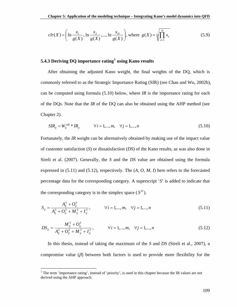
Chapter 5: Application of the modeling technique – Integrating Kano’s model dynamics into QFD
⎟⎟⎠
⎞⎜⎜⎝
⎛=
)(ln,...,
)(ln,
)(ln)( 21
Xgx
Xgx
XgxXclr D , where D
D
eexXg ∏
=
=1
)( (5.9)
5.4.3 Deriving DQ importance rating1 using Kano results
After obtaining the adjusted Kano weight, the final weights of the DQ, which is
commonly referred to as the Strategic Importance Rating (SIR) (see Chan and Wu, 2002b),
can be computed using formula (5.10) below, where IR is the importance rating for each
of the DQs. Note that the IR of the DQ can also be obtained using the AHP method (see
Chapter 2).
njmiIRWSIR ijadj
ijij ,...,1,,...,1* =∀=∀= (5.10)
Fortunately, the IR weight can be alternatively obtained by making use of the impact value
of customer satisfaction (S) or dissatisfaction (DS) of the Kano results, as was also done in
Sireli et al. (2007). Generally, the S and the DS value are obtained using the formula
expressed in (5.11) and (5.12), respectively. The (A, O, M, I) here refers to the forecasted
percentage data for the corresponding category. A superscript ‘S’ is added to indicate that
the corresponding category is in the simplex space ( ). DS
njmiIMOA
OAS S
ijSij
Sij
Sij
Sij
Sij
ij ,...,1,,...,1, =∀=∀+++
+= (5.11)
njmiIMOA
OMDS S
ijSij
Sij
Sij
Sij
Sij
ij ,...,1,,...,1, =∀=∀+++
+= (5.12)
In this thesis, instead of taking the maximum of the S and DS (Sireli et al., 2007), a
compromise value (β) between both factors is used to provide more flexibility for the
1 The term ’importance rating’, instead of ’priority’, is used in this chapter because the IR values are not derived using the AHP approach.
109

Chapter 5: Application of the modeling technique – Integrating Kano’s model dynamics into QFD
decision makers. The value of β, which ranges from 0 to 1, represents how much the
importance of achieving customer satisfaction as compared to avoiding customer
dissatisfaction. It may simply be obtained by asking the decision makers on the
importance of both factors. For example, if achieving customer satisfaction is three times
more important than avoiding customer dissatisfaction, then the value of β equals to 0.75.
Afterwards, the IR values for corresponding DQs can be obtained using expression (5.13).
( ) njmiDSSIR ijijij ,...,1,,...,1,*1* =∀=∀−+= ββ (5.13)
5.4.4 The Optimization Model
The purpose of the optimization model is to provide a more formal and systematic
process in designing multiple product using forecasted Kano data. As stated previously,
the model is very useful when the size of the QFD is relatively large, and reliance on
human efforts to do the selection process is virtually impossible. The objective of the
model is to allocate each DQ to the relevant product class as to maximize the strategic
importance rating (SIR) of each product in the corresponding class. The four generic
product classifications, namely, the basic product, the entry-level product, the advanced
product, and the high-end product, as proposed in Sireli et al. (2007), can be used as a
starting point for the example of product classes or variants.
Let p denote the number of product classes available {k=1,2,…, p}, then the customer
requirement for the i-th basic (must-have) feature with the j-th subcomponent can be
expressed as , which takes on binary value {0,1}, with ‘1’ indicating that the
corresponding DQ belongs to the k class and ‘0’ otherwise. The ‘quality’ of a particular
product class ( ) will be used to represent the contribution margin or the absolute profit
ijkDQ
kQ
110

Chapter 5: Application of the modeling technique – Integrating Kano’s model dynamics into QFD
per unit of each product class (Malik and Sullivan, 1995). Some criteria can be used to
determine the value or priority of each particular class’ ‘quality’ (Pollack-Johnson and
Liberatore, 2006), and the AHP (Saaty, 1980) is a useful tool in this respect. Finally, the
objective function of the model can be formulated as in (5.14).
∑∑∑= = =
=p
k
n
j
m
iijkkij DQQSIRZMax
1 1 1** , where { }1,0∈ijkDQ (5.14)
The above objective function may subject to several constraints. The main three
constraints will be described as follows:
a. Cost Limitation
With respect to budget allocation for each product class ( ), this cost limitation
constraint should be imposed in the model. For the corresponding DQ, a unit cost of
can be estimated and included in the constraint.
kB
ijC
pkBDQC k
n
j
m
iijkij ,...,1,*
1 1=∀≤∑∑
= =
(5.15)
b. Product Features Constraint
There are two types of features for this multiple product design problem as also
described previously, the first type is the basic or must-have feature, and the second type
is the subcomponent of the product features. However, for a chosen particular product
feature, one may not choose more than 1 subcomponent. For example, it does not make
sense to have two types of weight at the same time (‘ultra-light’ and ‘light’) for a laptop.
On the other hand, one may choose more than one kind of keyboard feature for a laptop,
for example, to have both ‘glowing’ and ‘spill-resistant’ features in a keyboard is perfectly
fine.
111

Chapter 5: Application of the modeling technique – Integrating Kano’s model dynamics into QFD
These conditions can be mathematically represented by the following two constraints:
∑=
=∀=∀=n
jijk pkmiDQ
1,...,1,,...,11 (5.16a)
pkmiDQn
jijk ,...,1,,...,1,1
1=∀=∀≥∑
=
(5.16b)
The mutually exclusive and collectively exhaustive condition are represented in (5.16a),
while the condition where there can be more than 1 subcomponent to be included is
expressed in (5.16b). In view of this, the QFD users may first decide which product
feature has the required property accordingly.
c. Product Class Constraint
In some cases, it is intuitively justifiable that one particular product feature can only
mapped into one particular product class, especially for the mutually exclusive product
feature. Constraint (5.17) imposes a limitation that a specific product feature is, at
maximum, allowed to be mapped into one product class.
∑=
=∀=∀≤p
kijk njmiDQ
1,...,1,,...,1,1 (5.17)
5.5 An illustrative example
To show the applicability of the proposed methodology, an example of a hypothetical
laptop design is used. Let suppose that a fictitious laptop company wants to design two
classes (p=2) of innovative feature-enhancing products for mobile computing, namely,
laptop ‘AA’ (high-end product) and laptop ‘AB’ (advanced product), simultaneously. For
the sake of simplicity, it is assumed that there are three main components or features,
those are, ‘weight’, ‘thickness’, and ‘keyboard’. Each of the main components is assumed
112

Chapter 5: Application of the modeling technique – Integrating Kano’s model dynamics into QFD
to have two subcomponents. The ‘weight’ component consists of two subcomponents,
namely, ‘ultra-light (±1 pound)’ (DQ11) and ‘light (±3 pounds)’ (DQ12). The ‘thickness’
component consists of ‘ultra-thin (±0.3 inches)’ (DQ21) and ‘thin (±0.6 inches)’ (DQ22),
and the ‘keyboard’ component consists of ‘glowing’ (DQ31) and ‘spill-resistant’ (DQ32).
It is clear that the subcomponents of the first two main components are mutually
exclusive and collectively exhaustive. For example, a laptop must have one type of weight,
and it is also impossible to have two types of thickness for one laptop. On the other hand,
a laptop may have more than one feature for its ‘keyboard’, which is the third main
component. In addition, for product differentiation purpose, it is decided that each of the
‘weight’ subcomponent can maximum be mapped into one particular class of product. In
other words, the two classes of laptop will not have the same weight.
5.5.1 Modeling Kano’s model dynamics
5.5.1.1 The input
It is assumed that a set of Kano questionnaire results, which was based on an online
survey conducted every two months for a certain group of customer, is already available.
The results from the last nine observations for each DQij are shown in the first left block
of Table 5.1-Table 5.3. It is worth noting that the typical Kano questionnaire results are in
percentage data form (see CQM, 1993 or Matzler and Hinterhuber, 1998). It describes the
percentage of the Kano categories for each customer attribute. For example, as shown in
Table 5.1, in the last period (t=9), there are 53% (A=0.53) of the customer surveyed
regarded DQ11 (ultra-light weight) as an attractive attribute.
113
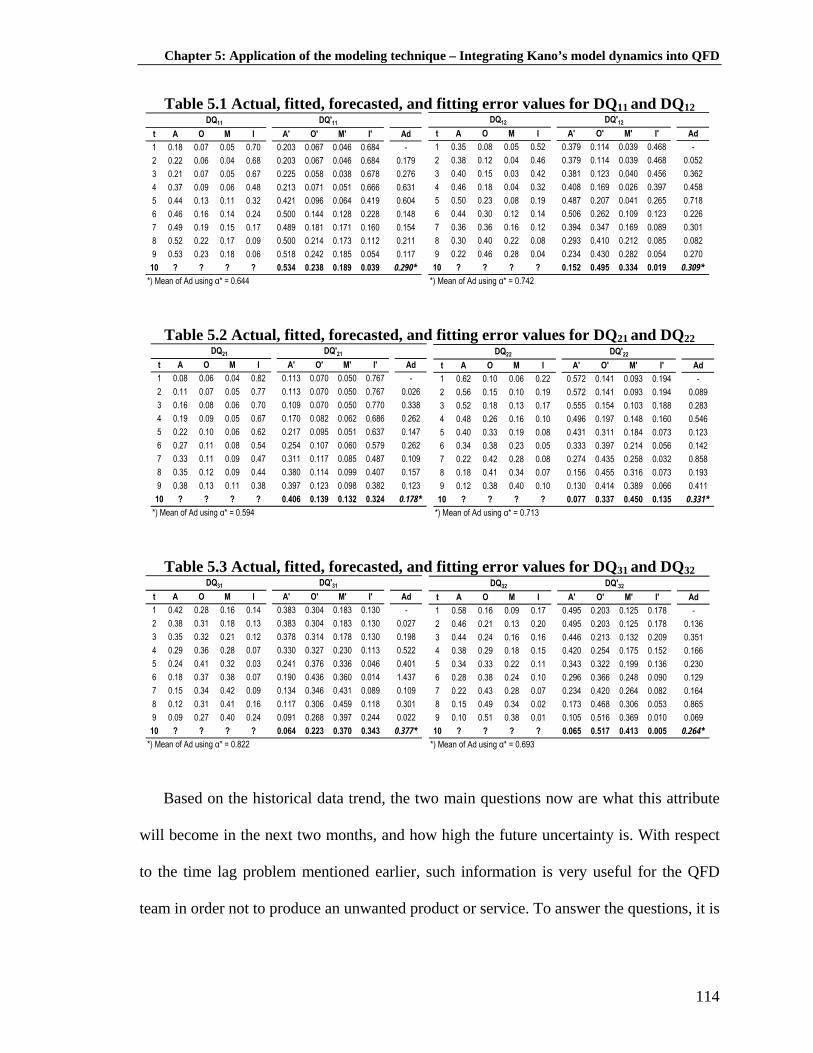
Chapter 5: Application of the modeling technique – Integrating Kano’s model dynamics into QFD
Table 5.1 Actual, fitted, forecasted, and fitting error values for DQ11 and DQ12
t A O M I A' O' M' I' Ad1 0.18 0.07 0.05 0.70 0.203 0.067 0.046 0.684 -2 0.22 0.06 0.04 0.68 0.203 0.067 0.046 0.684 0.1793 0.21 0.07 0.05 0.67 0.225 0.058 0.038 0.678 0.2764 0.37 0.09 0.06 0.48 0.213 0.071 0.051 0.666 0.6315 0.44 0.13 0.11 0.32 0.421 0.096 0.064 0.419 0.6046 0.46 0.16 0.14 0.24 0.500 0.144 0.128 0.228 0.1487 0.49 0.19 0.15 0.17 0.489 0.181 0.171 0.160 0.1548 0.52 0.22 0.17 0.09 0.500 0.214 0.173 0.112 0.2119 0.53 0.23 0.18 0.06 0.518 0.242 0.185 0.054 0.11710 ? ? ? ? 0.534 0.238 0.189 0.039 0.290*
DQ11 DQ'11
*) Mean of Ad using α* = 0.644
t A O M I A' O' M' I' Ad1 0.35 0.08 0.05 0.52 0.379 0.114 0.039 0.468 -2 0.38 0.12 0.04 0.46 0.379 0.114 0.039 0.468 0.0523 0.40 0.15 0.03 0.42 0.381 0.123 0.040 0.456 0.3624 0.46 0.18 0.04 0.32 0.408 0.169 0.026 0.397 0.4585 0.50 0.23 0.08 0.19 0.487 0.207 0.041 0.265 0.7186 0.44 0.30 0.12 0.14 0.506 0.262 0.109 0.123 0.2267 0.36 0.36 0.16 0.12 0.394 0.347 0.169 0.089 0.3018 0.30 0.40 0.22 0.08 0.293 0.410 0.212 0.085 0.0829 0.22 0.46 0.28 0.04 0.234 0.430 0.282 0.054 0.27010 ? ? ? ? 0.152 0.495 0.334 0.019 0.309*
DQ12 DQ'12
*) Mean of Ad using α* = 0.742
Table 5.2 Actual, fitted, forecasted, and fitting error values for DQ21 and DQ22
t A O M I A' O' M' I' Ad1 0.08 0.06 0.04 0.82 0.113 0.070 0.050 0.767 -2 0.11 0.07 0.05 0.77 0.113 0.070 0.050 0.767 0.0263 0.16 0.08 0.06 0.70 0.109 0.070 0.050 0.770 0.3384 0.19 0.09 0.05 0.67 0.170 0.082 0.062 0.686 0.2625 0.22 0.10 0.06 0.62 0.217 0.095 0.051 0.637 0.1476 0.27 0.11 0.08 0.54 0.254 0.107 0.060 0.579 0.2627 0.33 0.11 0.09 0.47 0.311 0.117 0.085 0.487 0.1098 0.35 0.12 0.09 0.44 0.380 0.114 0.099 0.407 0.1579 0.38 0.13 0.11 0.38 0.397 0.123 0.098 0.382 0.12310 ? ? ? ? 0.406 0.139 0.132 0.324 0.178*
DQ21 DQ'21
*) Mean of Ad using α* = 0.594
t A O M I A' O' M' I' Ad1 0.62 0.10 0.06 0.22 0.572 0.141 0.093 0.194 -2 0.56 0.15 0.10 0.19 0.572 0.141 0.093 0.194 0.0893 0.52 0.18 0.13 0.17 0.555 0.154 0.103 0.188 0.2834 0.48 0.26 0.16 0.10 0.496 0.197 0.148 0.160 0.5465 0.40 0.33 0.19 0.08 0.431 0.311 0.184 0.073 0.1236 0.34 0.38 0.23 0.05 0.333 0.397 0.214 0.056 0.1427 0.22 0.42 0.28 0.08 0.274 0.435 0.258 0.032 0.8588 0.18 0.41 0.34 0.07 0.156 0.455 0.316 0.073 0.1939 0.12 0.38 0.40 0.10 0.130 0.414 0.389 0.066 0.411
10 ? ? ? ? 0.077 0.337 0.450 0.135 0.331*
DQ22 DQ'22
*) Mean of Ad using α* = 0.713
Table 5.3 Actual, fitted, forecasted, and fitting error values for DQ31 and DQ32
t A O M I A' O' M' I' Ad1 0.42 0.28 0.16 0.14 0.383 0.304 0.183 0.130 -2 0.38 0.31 0.18 0.13 0.383 0.304 0.183 0.130 0.0273 0.35 0.32 0.21 0.12 0.378 0.314 0.178 0.130 0.1984 0.29 0.36 0.28 0.07 0.330 0.327 0.230 0.113 0.5225 0.24 0.41 0.32 0.03 0.241 0.376 0.336 0.046 0.4016 0.18 0.37 0.38 0.07 0.190 0.436 0.360 0.014 1.4377 0.15 0.34 0.42 0.09 0.134 0.346 0.431 0.089 0.1098 0.12 0.31 0.41 0.16 0.117 0.306 0.459 0.118 0.3019 0.09 0.27 0.40 0.24 0.091 0.268 0.397 0.244 0.02210 ? ? ? ? 0.064 0.223 0.370 0.343 0.377*
DQ31 DQ'31
*) Mean of Ad using α* = 0.822
t A O M I A' O' M' I' Ad1 0.58 0.16 0.09 0.17 0.495 0.203 0.125 0.178 -2 0.46 0.21 0.13 0.20 0.495 0.203 0.125 0.178 0.1363 0.44 0.24 0.16 0.16 0.446 0.213 0.132 0.209 0.3514 0.38 0.29 0.18 0.15 0.420 0.254 0.175 0.152 0.1665 0.34 0.33 0.22 0.11 0.343 0.322 0.199 0.136 0.2306 0.28 0.38 0.24 0.10 0.296 0.366 0.248 0.090 0.1297 0.22 0.43 0.28 0.07 0.234 0.420 0.264 0.082 0.1648 0.15 0.49 0.34 0.02 0.173 0.468 0.306 0.053 0.8659 0.10 0.51 0.38 0.01 0.105 0.516 0.369 0.010 0.06910 ? ? ? ? 0.065 0.517 0.413 0.005 0.264*
DQ32 DQ'32
*) Mean of Ad using α* = 0.693
Based on the historical data trend, the two main questions now are what this attribute
will become in the next two months, and how high the future uncertainty is. With respect
to the time lag problem mentioned earlier, such information is very useful for the QFD
team in order not to produce an unwanted product or service. To answer the questions, it is
114

Chapter 5: Application of the modeling technique – Integrating Kano’s model dynamics into QFD
necessary to first model the historical data of each DQ using the proposed compositional
double exponential smoothing (CDES) technique (see equation (5.1)-(5.5)).
5.5.1.2 Selection of model parameter
The average of the first three observations was used as the initial value. The optimal
value of the parameter, that is, the optimal smoothing constant (α*), was derived
iteratively by selecting a value between 0 and 1 that yields the smallest Aitchison distance
using a constant increment (see Section 5.3.3). The optimal alpha (α*) for each DQ, which
is used for fitting and forecasting, is shown below the actual data block column in Table
5.1-Table 5.3. For example, as shown in Table 5.1, the optimal alpha for DQ11 is 0.644
(α*=0.644).
The fitted, forecasted, and fitting error values are also shown in Table 5.1-Table 5.3,
next to the actual data block column for each corresponding DQ. The fitted values using
the CDES method are those values from t=1 until t=9 under the heading ‘DQ'11’ (with
prime), while the forecasted values are shown in the bolded values. For example, for DQ11
(Table 5.1), when t=9, the fitted value for the attractive attribute is 51.8% (A'=0.518), as
compared to the actual value which is 53% (A=0.53). The forecasted value is equal to
53.4% (A'=0.534, bolded), that is, the value when t=10.
5.5.1.3 Fitting error measurement
For each corresponding DQ, the last column of Table 5.1-Table 5.3, under the heading
‘Ad’, shows the fitting error values which are obtained using Aitchison distance (see
equation (5.6)). For example, when t=9, the distance between the actual compositional
115

Chapter 5: Application of the modeling technique – Integrating Kano’s model dynamics into QFD
data and the fitted one is equal to 0.117 (Ad=0.117). It is also worth noting that the values
shown in the last row (t=10) under the heading ‘Ad’ is the average of the fitting error
values for the corresponding DQ, for example, the average fitting error values for DQ11 is
0.290.
5.5.1.4 Results’ interpretation
The graphical representation of the fitting and forecasting results is shown in Figure
5.1-Figure 5.3. A full triangle, diamond, square, and dot are used to denote the actual
historical data point for the attractive (A), one-dimensional (O), must-be (M), indifferent
(I) category, respectively. Dash and dotted lines are used to show the fitted and forecasted
data point for each DQ. Some realistic descriptions of the DQs change over time are given
as follows.
DQ11
0.0
0.1
0.2
0.3
0.4
0.5
0.6
0.7
0.8
1 2 3 4 5 6 7 8 9 10Time
Per
cent
age
A A' O O' M M' I I'DQ12
0.0
0.1
0.2
0.3
0.4
0.5
0.6
1 2 3 4 5 6 7 8 9 10Time
Per
cent
age
A A' O O' M M' I I'
Figure 5.1 Graph of actual, fitted, and forecasted values for DQ11 and DQ12
DQ21
0.0
0.1
0.2
0.3
0.4
0.5
0.6
0.7
0.8
0.9
1 2 3 4 5 6 7 8 9 10Time
Per
cent
age
A A' O O' M M' I I'DQ22
0.0
0.1
0.2
0.3
0.4
0.5
0.6
0.7
1 2 3 4 5 6 7 8 9 10Time
Per
cent
age
A A' O O' M M' I I'
Figure 5.2 Graph of actual, fitted, and forecasted values for DQ21 and DQ22
116

Chapter 5: Application of the modeling technique – Integrating Kano’s model dynamics into QFD
DQ31
0.0
0.1
0.2
0.3
0.4
0.5
1 2 3 4 5 6 7 8 9 10Time
Per
cent
age
A A' O O' M M' I I'
DQ32
0.0
0.1
0.2
0.3
0.4
0.5
0.6
0.7
1 2 3 4 5 6 7 8 9 10Time
Per
cent
age
A A' O O' M M' I I'
Figure 5.3 Graph of actual, fitted, and forecasted values for DQ31 and DQ32
Initially, an ultra-light laptop (DQ11), was not attractive to the customers. The
customers are indifferent of this attribute for quite some time. This might be a common
phenomenon for some customers who receive new features of product, which is also
supported in the empirical study by Witell and Fundin (2005). However, starting from the
fourth period, it gradually becomes an attractive attribute since the customers started to
realize the significance of an ultra-light laptop (Figure 5.1). This change might be subject
to a number of factors, which is beyond the scope of this thesis, such as competitors’
products. Such situation also applies to DQ12 (light), but with a faster change. After the
fifth period, the DQ12 started to become obsolete. Then, beginning from the seventh period,
as can be observed in Figure 5.1, it becomes one-dimensional attribute. There is also an
inclination to become a must-be attribute in the end of the observation.
For ‘thickness’ component, initially, an ultra-thin size (DQ21), appears to be neutral for
the customers. In other words, most of the customers are indifferent with this attribute as
they might not be able to appreciate this (see Figure 5.2). This is not the case for the ‘thin’
size (DQ22), which was initially attractive, it quickly becomes one-dimensional. As the
passage of time, more and more customers begin to realize the importance of a thinner
laptop for mobile computing. Based on the trend in the change pattern, the forecasted
117

Chapter 5: Application of the modeling technique – Integrating Kano’s model dynamics into QFD
values for period ten (t=10) show that the ‘ultra-thin’ size will become an attractive
attribute, and the ‘thin’ size will become a must-be attribute.
As for the ‘keyboard’, the ‘glowing’ feature (DQ31) appears to have an exceptionally
fast rate of obsolescence. It was initially an attractive attribute, but it has become a must-
be attribute within a few periods (see Figure 5.3). Moreover, as shown in the forecasted
values (Table 5.3), this attribute might become an indifferent attribute in the future. In
contrast to DQ31, the ‘spill-resistant’ (DQ32) seems to have a relatively slow rate of change
(Figure 5.3). In the first four periods, it was an attractive attribute. However, it slowly
becomes one-dimensional attribute. Subsequently, it shows an inclination to become a
must-be attribute in the future.
5.5.2 Kano optimization for multiple product design
The main input for the optimization stage is the results from the forecasting stage
(Section 5.5.1). The objective of this optimization stage is to allocate each DQ to the
relevant product class as to maximize the strategic importance rating (SIR) of each
product in the corresponding class (see equation (5.14)). To obtain the SIR value for each
DQ, there are several steps to be taken as expressed in equation (5.7)-(5.13). The
necessary information for deriving the SIR value is shown in Table 5.4. Superscripts ‘S’
and ‘R’ are used to indicate, respectively, the forecasted Kano percentage data and the
transformed forecasted Kano percentage data. In other words, the results from the
previous section are those values under the heading ‘AS’, ‘OS’, ‘MS’, ‘IS’, for the
corresponding DQ.
118

Chapter 5: Application of the modeling technique – Integrating Kano’s model dynamics into QFD
Table 5.4 Input data for optimization model AS OS MS IS Gx AR OR MR IR δR
Weight ultra-light DQ11 0.534 0.238 0.189 0.039 0.18 1.11 0.31 0.07 -1.49 1.09light DQ12 0.152 0.495 0.334 0.019 0.15 0.03 1.21 0.82 -2.06 1.46
Thickness ultra-thin DQ21 0.406 0.139 0.132 0.324 0.22 0.61 -0.47 -0.52 0.38 0.58thin DQ22 0.077 0.337 0.450 0.135 0.20 -0.95 0.53 0.82 -0.39 0.82
Keyboard glowing DQ31 0.064 0.223 0.370 0.343 0.21 -1.17 0.08 0.58 0.51 0.81spill-resistant DQ32 0.065 0.517 0.413 0.005 0.09 -0.33 1.74 1.52 -2.93 2.17
Cat WKN sKN Wadj Sij DSij IRβ=.7 SIRij Cij
Weight ultra-light DQ11 A 9 0.21 9.88 0.77 0.43 0.67 6.61 12light DQ12 O 5 0.21 6.24 0.65 0.83 0.70 4.38 8
Thickness ultra-thin DQ21 A 9 0.10 9.48 0.54 0.27 0.46 4.38 5thin DQ22 M 3 0.26 3.55 0.41 0.79 0.53 1.87 3
Keyboard glowing DQ31 M 3 0.46 3.35 0.29 0.59 0.38 1.27 7spill-resistant DQ32 O 5 0.26 6.91 0.58 0.93 0.69 4.74 4
5.5.2.1 Deriving weights from the forecasted Kano percentage data
Based on the forecasted Kano percentage data, one needs to first determine to which
category a DQ belongs. For example, for the case of DQ11, since its attractive category has
the largest value (AS=0.534), then it belongs to attractive attribute. Thus, a ratio scale
weight of ‘9’ is assigned to this DQ ( , see equation (5.7)). Afterwards, this
weight is adjusted by two factors to improve its robustness.
911 =KNW
5.5.2.2 Deriving adjusted weights
The first factor, namely, the forecast-based variability ( ), can be obtained by
computing the standard deviation of the fitting values error for the corresponding DQ. The
resulting values of this factor for the laptop design example is shown in Table 5.4 under
the heading ‘SKN’. Note that the data used to derive the are the same as those that are
used to compute the mean of the Aitchison distance (‘Ad’) in Table 5.1-Table 5.3.
KNijs
KNijs
119

Chapter 5: Application of the modeling technique – Integrating Kano’s model dynamics into QFD
To compute the second factor, which is the degree of discrimination ( ), a
transformation of the forecasted percentage Kano data is needed. Using formula (5.9), the
transformed percentage data are shown in Table 5.4 under the heading ‘AR’, ‘OR’, ‘MR’,
‘IR’. The superscript ‘R’ is used to indicate that the values are in the real space (
Rijδ
ℜ ). The
‘Gx’ column (Table 5.4) denotes the geometric mean of the forecasted Kano percentage
data. The degree of discrimination values for this example data are shown in Table 5.4
under the heading ‘ ’. Rδ
The adjusted Kano weight ( ) is obtained using formula (5.8). For the sake of
simplicity, the trade-off values of the adjusting factors are assumed to be the same
( = =1). The resulting values of the adjusted weight are shown in Table 5.4 under the
heading ‘Wadj’.
adjijW
dijλ
sijλ
5.5.2.3 Deriving DQ importance rating using Kano results
Since the SIR value is the product of the adjusted weight ( ) and the importance
rating (IR) (see formula (5.10)), then the IR values need to be computed. For simplicity, it
is again assumed that a compromise value of 0.7 (β=0.7) is used for the importance of
customer satisfaction (S) as compared to customer dissatisfaction (DS). Using equation
(5.11)-(5.13), the , , and the IR values can be derived. The resulting values are
shown in Table 5.4, respectively, under the heading ‘Sij’, ‘DSij’, and ‘IRβ=.7’. The final
SIR values are also shown in Table 5.4, under the heading ‘SIRij’.
adjijW
ijS ijDS
120
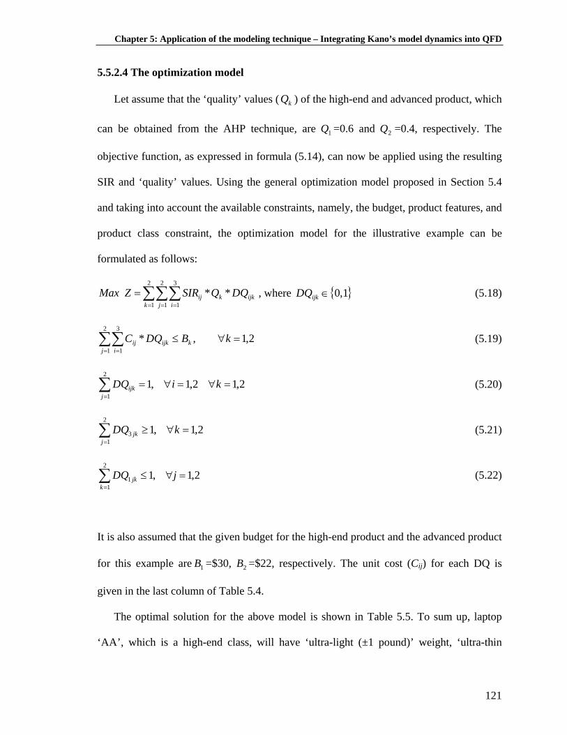
Chapter 5: Application of the modeling technique – Integrating Kano’s model dynamics into QFD
5.5.2.4 The optimization model
Let assume that the ‘quality’ values ( ) of the high-end and advanced product, which
can be obtained from the AHP technique, are =0.6 and =0.4, respectively. The
objective function, as expressed in formula (5.14), can now be applied using the resulting
SIR and ‘quality’ values. Using the general optimization model proposed in Section 5.4
and taking into account the available constraints, namely, the budget, product features, and
product class constraint, the optimization model for the illustrative example can be
formulated as follows:
kQ
1Q 2Q
∑∑∑= = =
=2
1
2
1
3
1**
k j iijkkij DQQSIRZMax , where { }1,0∈ijkDQ (5.18)
2,1,*2
1
3
1
=∀≤∑∑= =
kBDQC kj i
ijkij (5.19)
∑=
=∀=∀=2
1
2,12,1,1j
ijk kiDQ (5.20)
2,1,12
13 =∀≥∑
=
kDQj
jk (5.21)
∑=
=∀≤2
11 2,1,1
kjk jDQ (5.22)
It is also assumed that the given budget for the high-end product and the advanced product
for this example are =$30, =$22, respectively. The unit cost (Cij) for each DQ is
given in the last column of Table 5.4.
1B 2B
The optimal solution for the above model is shown in Table 5.5. To sum up, laptop
‘AA’, which is a high-end class, will have ‘ultra-light (±1 pound)’ weight, ‘ultra-thin
121

Chapter 5: Application of the modeling technique – Integrating Kano’s model dynamics into QFD
(±0.3 inches)’ thickness, and both of the keyboard features, while laptop ‘AB’, which is an
advanced class, will have ‘light (±3 pounds)’ weight, ‘ultra-thin (±0.3 inches)’ thickness,
and only ‘spill-resistant’ feature for the keyboard.
Table 5.5 Multiple product design optimization results
DQ ijk (i =1, j =1) (i =1, j =2) (i =2, j =1) (i =2, j =2) (i =3, j =1) (i =3, j =2)
k =1 1 0 1 0 1 1k =2 0 1 1 0 0 1
5.6 Conclusion
The purpose of this chapter was to demonstrate one application of the new modeling
technique (Chapter 4) as to improve QFD analysis. The modeling technique has been
shown to be effective in formally modeling the dynamics of Kano’s model so that one
may know how fast the change over time is. Monitoring the change of quality attributes
(Kano’s model attributes) over time may not only help strengthen the QFD input by
providing a timely update of customer’s needs information, but may also be useful for
tackling the problem described in Chapter 1.
Furthermore, based on the results of the Kano’s model dynamics modeling phase, a
further QFD analysis that extends the research on using Kano’s model in QFD for
multiple product design (Sireli et al., 2007) has also been suggested. Specifically, the
extension is two-fold. One is to suggest the use of the optimization model, which is
particularly useful when the number of DQs is relatively large. The other is to improve the
robustness of the results by incorporating two sources of variability, namely, forecast-
based variability and within category variability of the forecasted data.
122

Chapter 5: Application of the modeling technique – Integrating Kano’s model dynamics into QFD
123
For future works, there are two interesting issues that may be worth investigating. First,
it is the incorporation of modular product design concept into the multiple product design
process in QFD. The use of modular design concept in QFD, although it is quite limited,
can be found in Kreng and Lee (2004) or Takai, (2006). Second, it is a further
investigation on the relationship between Kano’s model dynamics and the innovation
adoption framework or life cycle (Rogers, 2003). For example, a certain high-tech product
feature may already be regarded as a must-be attribute by the early market innovators,
while it may still be perceived as an attractive one by the late majority market. Thus,
further research on how this issue be taken into account in the design process might be
worth pursuing.
In sum, this chapter has not only extended the use of Kano’s model in QFD analysis,
but it has also advanced the academic literature on modeling the life cycle of quality
attributes quantitatively. To further demonstrate the usefulness of the new modeling
technique (Chapter 4), the next chapter (Chapter 6) will describe another application of the
technique in improving QFD analysis, that is, in enhancing the benchmarking analysis of
QFD with respect to the problem described in Chapter 1.

Chapter 6: Application of the modeling technique – Dynamic benchmarking in QFD
CHAPTER 6
APPLICATION OF THE MODELING TECHNIQUE (PART 2 OF 2) –
DYNAMIC BENCHMARKING IN QFD
The purpose of this chapter is to demonstrate another application of the new modeling
technique (Chapter 4) as to improve QFD analysis. The modeling technique will be
applied to model the change of DQs’ competitive assessment over time, apart from the
DQs’ priorities. As mentioned previously (Section 1.1), another important change during
product or service creation process is the change of competitive assessment of the DQs.
This is due to fact that the competitors’ performance naturally changes over time.
Therefore, to improve the likelihood of success of a QFD application, such factor may not
be overlooked. In other words, it is important to keep pace with the change when
formulating competitive strategies. This chapter provides the way to integrate both the
dynamics of DQs’ priorities and DQs’ competitive assessment, along with their interaction,
in a QFD analysis. This chapter is reproduced from “Dynamic Benchmarking
Methodology for QFD”, by Raharjo H, Chai KH, Xie M, Brombacher AC. To appear in
Benchmarking: An International Journal.
6.1 Introduction
A competitive advantage, generally, can be gained if a company produces a product
that not only addresses what the customer values most, but also performs better than its
competitors in terms of quality, cost, and timeliness. However, these two factors, namely,
the customer needs and competitors’ performance, change over time, and yet there are still
a number of product design processes that seem to have oversimplified this fact. In the
124

Chapter 6: Application of the modeling technique – Dynamic benchmarking in QFD
QFD literature, the former factor has been quite well addressed, for example, see Shen et
al. (2001), Xie et al. (2003), Wu et al. (2005), Wu and Shieh (2006), Raharjo et al. (2006).
Unfortunately, there is too little attention paid to the latter, which is equally critical. To
design or upgrade a product successfully using QFD, it may not be sufficient to only
observe the change of DQs’ priorities over time because during the product creation
process, competitive condition, especially, competitors’ performance changes as well.
Therefore, to improve the likelihood of success of a product design or upgrade process,
both of these factors and their dynamics should be taken into account.
This chapter aims to address this issue, that is, how the dynamics of these two factors
along with their interaction can be integrated into a QFD analysis. For simplicity, the
suggested approach is referred to as dynamic benchmarking methodology. The
methodology essentially comprises of two novel approaches. First, it is the use of the new
modeling technique, as described in Chapter 4, to model the trend of DQs’ priorities and
their competitive assessment. Note that, in contrast to the traditional practice which mostly
uses a direct rating scale of, for example, 1-to-5 or 1-to-9 (Hauser and Clausing, 1988;
Cohen, 1995), the importance rating values and the competitors’ benchmarking
information are obtained using the AHP’s relative measurement. Second, it is the
approach, which is called the strength-weakness-opportunity-threat (SWOT)-based
competitive weighting scheme, to derive weights by analyzing the interaction between the
two factors. In addition, this proposed weighting scheme also serves as a more systematic
way to substitute the traditional QFD customer competitive target setting and sales point
value determination.
The following sections are organized as follows. Section 6.2 will describe the need of
dynamic benchmarking in QFD based on what have been done in the literature. Then, the
125

Chapter 6: Application of the modeling technique – Dynamic benchmarking in QFD
proposed benchmarking methodology is elaborated in Section 6.3. To illustrate how the
proposed methodology works practically, an illustrative example is provided (Section 6.4).
Section 6.5 will elaborate how the competitive weighting scheme is used to derive the
final DQ’s weight, namely, the strategic importance rating (Chan and Wu, 2002b), by
considering the two factors’ interaction. Finally, the novel contribution and possible
extensions are discussed (Section 6.6).
6.2 The need of dynamic benchmarking: literature review and research
gap
A benchmarking process can be regarded as a continuous and proactive search for the
best practices leading to a superior performance of a company (Camp, 1995). Successful
benchmarking may lead to an improved return on investment ratio, increased market
competitiveness, cost reductions, higher chance of identifying new business opportunities,
and enhanced transparency and performance (Ramabadran et al., 2004; Braadbaart, 2007).
It provides insights necessary to effectively pinpoint the critical success factors that set the
most successful firms apart from their competitors, or to a greater extent, that separates the
winners from the losers (Cooper and Kleinschmidt, 1987, 1995). Specifically, the
benchmarking information can serve as a foundation for a company to formulate strategic
decisions effectively (Spendolini, 1992).
An important fact worth highlighting is that, as the passage of time, the company as
well as the competitors’ condition will certainly change. Therefore, benchmarking process
should not remain static. The importance of dynamic benchmarking has been realized by
several researchers. Min et al. (1997) used the AHP for competitive benchmarking and
126

Chapter 6: Application of the modeling technique – Dynamic benchmarking in QFD
substantiated the need of dynamic benchmarking that is capable of evaluating the
changing degree of clinic’s patient satisfaction over time. In attempt to identify tools,
methodologies, and metrics that can serve as enablers for making benchmarking in agile
environments effective and efficient, Sarkis (2001) highlighted the importance of forward
thinking (proactive) approach in benchmarking, such as by using forecasting techniques,
on the basis of historical data, to obtain future benchmarks.
Min et al. (2002) analyzed the changing hotel’s customer needs over time and
demonstrated the importance of dynamic benchmarking to strive for continuous service
quality improvement. Unfortunately, they only focused on two data points in time, namely,
year 1995 and year 2000, which is very likely inadequate for observing the change over
time. Salhieh and Singh (2003) proposed a dynamic framework using principles of
systems dynamics to incorporate benchmarking for university effective policy design.
However, their approach can be considered ‘reactive’ since they relied on a feedback
mechanism. Tavana (2004) proposed a dynamic benchmarking framework, which uses the
AHP and additive Multiple Criteria Decision Making (MCDM) model, for technology
assessment at NASA.
In the existing QFD literature, the issue of benchmarking has been, to some extent,
oversimplified. Some previous attempts can be found in Lu et al. (1994), Ghahramani and
Houshyar (1996), Gonzáles et al. (2005), Iranmanesh et al. (2005), or Ginn and Zairi,
(2005). Using a real world case study, Kumar et al. (2006) demonstrated that there is a
synergistic effect in integrating benchmarking with QFD methodologies for companies
that seek higher levels of financial and strategic performance through product
improvement. Gonzáles et al. (2008) demonstrated the effective application of QFD and
benchmarking to enhance academic programmes. More recently, Lai et al. (2008) showed
127

Chapter 6: Application of the modeling technique – Dynamic benchmarking in QFD
the importance of competitor information for deriving QFD’s customer requirements
ranking. With respect to this, they developed a new ranking method that is based on fuzzy
mathematics.
Nevertheless, almost none of the existing studies have adequately addressed the need
to provide a more formal and systematic approach to use dynamic benchmarking in QFD.
As mentioned previously, the competitive condition may change during product creation
process, therefore how to appropriately deal with such change is of great necessity.
Pursuing the ‘proactive’ stream of research in dealing with the market dynamics, as first
initiated by Shen et al. (2001) or Xie et al. (2003), this chapter attempts to fill in this gap
by proposing the use of a forecasting technique for monitoring, apart from the change of
customer preferences (DQs’ priorities), the change of the benchmarking information
(DQs’ competitive assessment) in the QFD.
It is worth noting that the AHP’s relative measurement is suggested for deriving both
DQs’ priorities and their competitive assessment. Examples of the use of the AHP-based
approach for benchmarking can be found in Korpela and Tuominen (1996), Min et al.
(1997), Chan et al. (2006), Chen and Huang (2007), Dey et al. (2008), Tavana (2008) or
Raharjo et al. (2008). In the end, it is expected that having known the timely update of
information on the change of competitors’ performance and the change of customer
preference over time, along with their interaction, the QFD decision making process may
be improved.
128

Chapter 6: Application of the modeling technique – Dynamic benchmarking in QFD
6.3 The proposed dynamic benchmarking methodology
This section describes the proposed dynamic benchmarking methodology for QFD.
Section 6.3.1 provides necessary information on how one may obtain the input data from
the customer through the use of the AHP. Then, the step-by-step procedure to use the
proposed methodology is elaborated in Section 6.3.2.
6.3.1 The input
Similar to most methodologies in benchmarking, the input of the proposed dynamic
benchmarking methodology mainly relies on the customer data of a specific market
segment. The customer’s opinion or judgment is required to assess the importance of a
DQ and how well the company and the competitors satisfy it. Traditionally, those data,
namely, the importance rating and the customer competitive assessment are obtained
based on a direct rating of 1 to 5. Such approach might very likely lead to a tendency for
the customers to assign values near to the highest possible scores, and eventually result in
somewhat arbitrary and inaccurate results (Cohen, 1995; Chuang, 2001).
To remedy this problem, some researchers proposed the use of the AHP for eliciting
the importance rating (see Chapter 2). However, there appears to have been almost no
study to improve the judgment elicitation process for the benchmarking part or the DQs’
competitive assessment. A better and more rigorous approach is needed to avoid the
weakness of the traditional approach. Therefore, the AHP approach is proposed to be used
as a tool to elicit customer’s judgments not only for the importance rating part (DQs’
priorities), but also for the benchmarking part (DQs’ competitive assessment).
129

Chapter 6: Application of the modeling technique – Dynamic benchmarking in QFD
As prescribed in the AHP procedure, the judgments are elicited using the pairwise
comparison question (Saaty, 1994). For the DQ’s priority part, the following question can
be used:
• “With respect to the design of the (new) product, how important is the first DQ
(DQ1) compared to the second DQ (DQ2)?”
While for the benchmarking part, the following question can be used:
• “With respect to DQ1, how good is the performance of Competitor1 compared
to Competitor2?”
Note that these questions can be tailored to suit a particular condition of the problem at
hand.
The key point here is that, in assessing the competitors’ performance in the HoQ, this
AHP approach is much more relevant compared to the standard rating approach, such as
using a scale of 1 to 5 (Cohen, 1995). This is because the AHP uses a relative
measurement while the rating approach uses an absolute measurement. In the context of
DQs’ competitive assessment, a ‘good’ performance, to some extent, is determined
relatively by the performance of ‘best-in-class’ competitors. As pointed out by Lai et al.
(2008), a company may perform poorly in meeting a particular DQ, however, if its
competitors are not as good, it might stand out in the market although the customer
satisfaction level is relatively low. In other words, how good the performance of a
company on a certain DQ is depends relatively on other companies’ performance on the
same DQ. Thus, this clearly shows the relevance of the AHP’s relative measurement.
The results of the pairwise comparisons are the priorities of the entities being
compared in ratio-scale (Harker and Vargas, 1987). As has been mentioned previously, if
130

Chapter 6: Application of the modeling technique – Dynamic benchmarking in QFD
the judgment elicitation is carried out every month, it is most likely that the priorities will
change over time. Now, how to make use of this information for improving QFD analysis
is the question that this chapter attempts to answer. The forecasting method described in
Chapter 4, namely, the compositional double exponential smoothing (CDES) technique,
will be used to model the priorities’ change over time.
6.3.2 The step-by-step procedure
The following step-by-step procedure is suggested to be used for the proposed
dynamic benchmarking methodology.
Step 1: Obtain the DQs’ priorities from the customer using the AHP procedure.
Step 2: Obtain the customer competitive assessment on our product compared to the ‘best-
in-class’ competitors in the industry using the AHP procedure. This type of
benchmarking can be considered as the competitive or external benchmarking
(Zairi, 1992; Madu and Kuei, 1993; Camp, 1995).
Step 3: Record the priorities and collect data periodically for a certain length of time, for
example, every month until nine months.
Step 4: Model the priorities change over time, and obtain a forecast.
Step 5: Obtain forecasted values of both the DQs’ priorities and DQs’ competitive
assessment. These forecasted values basically reflect the future voice of the
customer. They should be used for the QFD input at least because of two reasons.
One is to avoid the time-lag problem (see Chapter 1). The other is to design a
new or to upgrade an existing product to meet the future needs of the customer
while considering the future competitors’ performance.
131

Chapter 6: Application of the modeling technique – Dynamic benchmarking in QFD
Step 6: Conduct competitive analysis using the proposed competitive weighting scheme
(see Section 6.5)
Step 7: Obtain the final priorities of the DQs, namely, the strategic importance rating
(SIR).
It is worth noting that, for Step 2, it is of critical importance to correctly select
the ’best-in-class’ competitors since failing to do so may lead to an inferior outcome of the
benchmarking endeavor. If the competitor’ class is too high, the company will never
achieve the unrealistically high target, and will likely end up in frustration. On the other
hand, if the company compares itself to a competitor of much lower tier, then the company
will never improve, but remain in a state of complacency.
The ’best-in-class’ may imply that they share at least similar price classification and
market segment. Shen et al. (2000) proposed an intuitively interesting way to develop this
idea, that is, to use hierarchical benchmarks for strategic competitor selection. For
example, after being able to reach local-class standard, the company should strive for
higher class (regional-class) and gradually moving towards world-class performance. In
the case when a company is already perceived as a world-class company, it does not then
mean that the company cannot improve themselves since there is always a better way to
do things.
6.4 An illustrative example
To illustrate the proposed approach, consider the following example. Suppose that
there are three DQs being monitored. It is assumed that the historical data for a period of
132

Chapter 6: Application of the modeling technique – Dynamic benchmarking in QFD
nine months for the DQs’ priorities and the competitive assessment priorities are already
available. These data are generated from a simulation of AHP reciprocal matrices using
the fundamental scale of 1-to-9 (see Section 4.2.1.2). All the generated matrices have
consistency ratio value of less than 0.1. For the sake of simplicity, it is assumed that there
is no problem in Step 1 and Step 2.
6.4.1 The input
Step 3: The DQs’ priorities (IR values) for the last nine periods are shown in Table 6.1.
For example, in the first period (t=1), DQ1 is regarded by the customer as the most
important attribute (0.667), while the other DQs are not that important. On the other hand,
in the last period (t=9), DQ3 becomes the most important attribute (0.413). Note that the
DQs’ priorities in a certain period always sum up to unity because of the AHP procedure
which uses normalization.
Table 6.1 DQs’ priorities (IR values) over time
t DQ1 DQ2 DQ3 DQ'1 DQ'2 DQ'3 Err (Ad)1 0.667 0.222 0.111 0.647 0.230 0.123 -2 0.648 0.230 0.122 0.647 0.230 0.123 0.00523 0.625 0.238 0.136 0.648 0.230 0.122 0.10314 0.540 0.297 0.163 0.623 0.239 0.138 0.27485 0.493 0.311 0.196 0.521 0.308 0.172 0.13446 0.550 0.240 0.210 0.454 0.332 0.214 0.36707 0.413 0.327 0.260 0.518 0.247 0.236 0.36398 0.333 0.333 0.333 0.385 0.324 0.291 0.19969 0.327 0.260 0.413 0.284 0.340 0.376 0.3171
10 forecast 0.309 0.197 0.4950.1322a*=0.57, Err StDev=
IR IR
The data which are shown next to the original data block column are the fitted data
and the forecast result using the CDES technique (Chapter 4). For example, the forecasted
133

Chapter 6: Application of the modeling technique – Dynamic benchmarking in QFD
priorities for DQ1, DQ2, and DQ3, respectively, in the coming period (t=10), are 0.309,
0.197, and 0.495. A more detailed explanation of the figures in Table 6.1 will be provided
in the next subsection.
The DQs’ competitive assessment priorities, which are also obtained using the AHP,
of the company (Z) and the two best-in-class competitors, namely, competitor A and
competitor B, for each DQ are shown in Table 6.2 to Table 6.4. For example, in Table 6.2,
the customer of the specific segment in the first period (t=1) perceived that company B
performs the best (0.413) as relatively compared to the other companies. However, in the
last period (t=9), company A was perceived as the best one (0.558). The fitted and
forecasted data in Table 6.2 to Table 6.4 will be explained in the next subsection.
Table 6.2 Customer competitive assessment over time for DQ1
t Z A B Z' A' B' Err(Ad)1 0.260 0.327 0.413 0.284 0.358 0.358 -2 0.333 0.333 0.333 0.284 0.358 0.358 0.18843 0.260 0.413 0.327 0.341 0.330 0.330 0.35024 0.500 0.250 0.250 0.264 0.417 0.319 0.85165 0.413 0.260 0.327 0.524 0.243 0.234 0.40576 0.260 0.327 0.413 0.467 0.230 0.303 0.74797 0.200 0.400 0.400 0.261 0.310 0.429 0.37238 0.169 0.443 0.387 0.169 0.408 0.423 0.12249 0.122 0.558 0.320 0.134 0.472 0.394 0.2714
10 forecast 0.084 0.665 0.2520.2578α*=0.57, Err StDev=
DQ1 DQ1
Table 6.3 Customer competitive assessment over time for DQ2
t Z A B Z' A' B' Err(Ad)1 0.500 0.250 0.250 0.414 0.304 0.282 -2 0.413 0.327 0.260 0.414 0.304 0.282 0.10813 0.333 0.333 0.333 0.413 0.326 0.261 0.32514 0.327 0.260 0.413 0.336 0.339 0.324 0.35875 0.250 0.250 0.500 0.310 0.267 0.423 0.27276 0.140 0.333 0.528 0.233 0.235 0.532 0.60767 0.163 0.297 0.540 0.123 0.298 0.578 0.26188 0.109 0.309 0.582 0.123 0.290 0.587 0.12989 0.097 0.333 0.570 0.088 0.297 0.615 0.1481
10 forecast 0.086 0.357 0.5570.1627α*=0.48, Err StDev=
DQ2 DQ2
134

Chapter 6: Application of the modeling technique – Dynamic benchmarking in QFD
Table 6.4 Customer competitive assessment over time for DQ3
t Z A B Z' A' B' Err(Ad)1 0.260 0.413 0.327 0.240 0.380 0.380 -2 0.260 0.327 0.413 0.240 0.380 0.380 0.19023 0.200 0.400 0.400 0.258 0.332 0.410 0.31174 0.250 0.500 0.250 0.209 0.382 0.409 0.58815 0.260 0.413 0.327 0.239 0.494 0.268 0.27466 0.210 0.550 0.240 0.258 0.448 0.294 0.33547 0.333 0.333 0.333 0.217 0.550 0.233 0.73238 0.413 0.260 0.327 0.318 0.382 0.300 0.47289 0.400 0.200 0.400 0.425 0.259 0.316 0.3501
10 forecast 0.378 0.149 0.4730.1792
DQ3 DQ3
α*=0.45, Err StDev=
6.4.2 The process
Step 4: The CDES method (Chapter 4) is adopted to model the change of the AHP
priorities over time and to obtain a forecast. The results of the fitting process and the
forecasted priorities for the DQs and their customer competitive assessment are shown in
Table 6.1-Table 6.4 (next to the original data block column).
All of the tables above (Table 6.1-Table 6.4) have two block-columns next to the
original data block-column. The first block-column, next to the original data, shows the
results of the fitting and forecasting process, while the second one shows the deviation
(error) between the original data and the fitted value. Note that the interpretation for these
two block-columns is the same for all the tables.
Take an example, in Table 6.4, the fitted values at t=9 for the company (Z), competitor
A, and competitor B, respectively, are Z’=0.425, A’=0.259, B’=0.316. These values are
obtained using the CDES technique described in Chapter 4. The initial values for the
CDES technique are obtained from the first three observations shown in Table 6.1 to
Table 6.4. The Aitchison distance is used as the measure of the difference between the
original data and the fitted data, that is, the forecasting error or residual. The forecasting
135
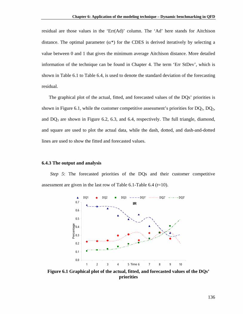
Chapter 6: Application of the modeling technique – Dynamic benchmarking in QFD
residual are those values in the ‘Err(Ad)’ column. The ‘Ad’ here stands for Aitchison
distance. The optimal parameter (α*) for the CDES is derived iteratively by selecting a
value between 0 and 1 that gives the minimum average Aitchison distance. More detailed
information of the technique can be found in Chapter 4. The term ‘Err StDev’, which is
shown in Table 6.1 to Table 6.4, is used to denote the standard deviation of the forecasting
residual.
The graphical plot of the actual, fitted, and forecasted values of the DQs’ priorities is
shown in Figure 6.1, while the customer competitive assessment’s priorities for DQ1, DQ2,
and DQ3 are shown in Figure 6.2, 6.3, and 6.4, respectively. The full triangle, diamond,
and square are used to plot the actual data, while the dash, dotted, and dash-and-dotted
lines are used to show the fitted and forecasted values.
6.4.3 The output and analysis
Step 5: The forecasted priorities of the DQs and their customer competitive
assessment are given in the last row of Table 6.1-Table 6.4 (t=10).
IR
0.0
0.1
0.2
0.3
0.4
0.5
0.6
0.7
1 2 3 4 5 6 7 8 9 10Time
Per
cent
age
DQ1 DQ2 DQ3 DQ1' DQ2' DQ3'
Figure 6.1 Graphical plot of the actual, fitted, and forecasted values of the DQs’
priorities
136
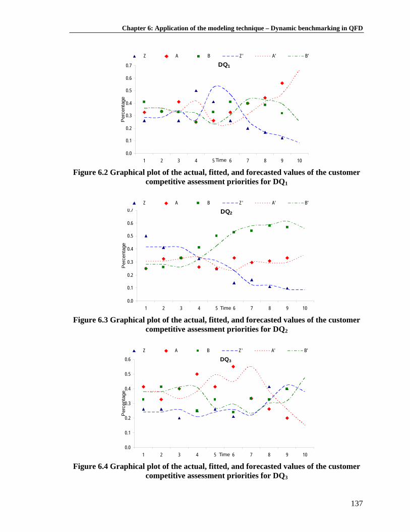
Chapter 6: Application of the modeling technique – Dynamic benchmarking in QFD
DQ1
0.0
0.1
0.2
0.3
0.4
0.5
0.6
0.7
1 2 3 4 5 6 7 8 9 10Time
Per
cent
age
Z A B Z' A' B'
Figure 6.2 Graphical plot of the actual, fitted, and forecasted values of the customer
competitive assessment priorities for DQ1
DQ2
0.0
0.1
0.2
0.3
0.4
0.5
0.6
0.7
1 2 3 4 5 6 7 8 9 10Time
Per
cent
age
Z A B Z' A' B'
Figure 6.3 Graphical plot of the actual, fitted, and forecasted values of the customer
competitive assessment priorities for DQ2
DQ3
0.0
0.1
0.2
0.3
0.4
0.5
0.6
1 2 3 4 5 6 7 8 9 10Time
Per
cent
age
Z A B Z' A' B'
Figure 6.4 Graphical plot of the actual, fitted, and forecasted values of the customer
competitive assessment priorities for DQ3
137

Chapter 6: Application of the modeling technique – Dynamic benchmarking in QFD
The graphical plot of the forecasting results for the customer competitive assessment for
each DQ is shown in Figure 6.5. The forecasted relative performance values for company
Z, competitor A, competitor B are denoted by the solid line, long-dash line, and dash line,
respectively. The forecasted priority for each DQ (forecasted IR value or ‘F.IR’) is
denoted by a full dot.
-0.10
0.10
0.30
0.50
0.70
0.90DQ'1
DQ'2DQ'3
ZABF.IR
Figure 6.5 The radar diagram portraying the future competitive assessment
It can be seen that with respect to DQ1 and DQ2, which will not become very
important attributes, the predicted performance of company Z is the lowest compared to
the others. While with respect to DQ3, which will become a very important attribute, the
predicted performance of company Z is between competitor A and competitor B. The
following section will show how the interaction of the two projected future conditions
may enhance the decision making process in the QFD analysis, particularly in determining
the strategic importance rating (SIR) of the customer needs (DQs).
138
Chapter 6: Application of the modeling technique – Dynamic benchmarking in QFD
6.5 The competitive weighting scheme: A SWOT-based approach
Taking into account the interaction between the forecasted DQs’ priorities, which may
reflect the future needs of the customer, and the forecasted priorities of the DQs’
competitive assessment, which may reflect the future performance of the competitors, a
competitive weighting scheme is proposed. The basic idea is to assign a multiplier to the
DQ based on the forecasting results obtained from previous section. As compared to the
traditional QFD, this approach may provide a more formal and systematic way for QFD
practitioners in carrying out the customer target setting and sales point determination in
the house of quality.
The proposed competitive weighting scheme is based on the idea of strength-
weakness-opportunity-threat (SWOT) analysis. The framework is shown graphically in
Figure 6.6. The x-axis denotes the forecasted competitors’ relative performance, while the
y-axis denotes the forecasted relative priority of a customer need (DQ). The weighting
scheme can basically be divided into four groups as follows:
1. Strength (I)
This case is for the situation when both the future competitors’ relative performance
and the future relative importance are rather low. In other words, the competitors’
performance will be relatively lower than that of the company on a less important
attribute. Thus, a multiplier value of 1 is assigned to this type of attribute. Note that
the term ‘less important’ here does not mean ‘unimportant’ since an unimportant
attribute will not be included in the DQ’s list.
139

Chapter 6: Application of the modeling technique – Dynamic benchmarking in QFD
2. Weakness (II)
This is for the situation when the competitors will relatively perform better than the
company on a relatively less important attribute. Thus, a multiplier value of 3 is
assigned. In the case when the competitors’ relative performance will be equally good
compared to the company, a multiplier value of 2 is assigned.
3. Opportunity (III)
This is for the situation when the future competitors’ relative performance will be
relatively lower than that of the company on a relatively more important attribute.
Thus, this case may be regarded as an opportunity for the company to differentiate
itself from the competitors. A multiplier value of 7 is assigned.
4. Threat (IV)
If the future competitors’ relative performance will be relatively better than the
company on a relatively more important attribute, then this signals a threat. The QFD
team should place a special attention to such case. Thus, a multiplier value of 9 is
assigned. A multiplier value of 8 can be assigned for the case when the future
competitors’ relative performance will be equally good compared to the company’s.
140

Chapter 6: Application of the modeling technique – Dynamic benchmarking in QFD
Figure 6.6 The proposed weighting scheme
For the in-between multiplier values other than described in the paragraph above, such
as, 4, 5, 6, a similar interpretation can be used accordingly. Take for an example, a
multiplier of 6 is assigned when the future competitors’ relative performance will be
relatively better than that of the company on a moderately important attribute. Table 6.5
shows the complete information on the proposed weighting scheme based on the x-axis
and the y-axis.
Table 6.5 The proposed competitive weighting scheme
IR CRP weight NoteLow Low 1 StrengthLow Medium 2 S-WLow High 3 WeaknessMedium Low 4 S-OMedium Medium 5 S-W-O-TMedium High 6 W-THigh Low 7 OpportunityHigh Medium 8 O-THigh High 9 Threat
The ‘IR’ here refers to the forecasted IR values of the customer attributes (DQs’
priorities), while the ‘CRP’ stands for the forecasted competitors’ relative performance. A
141
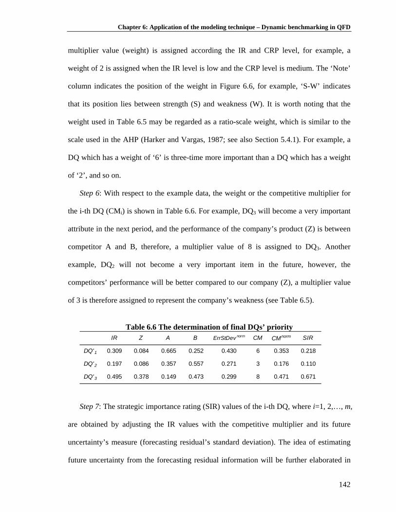
Chapter 6: Application of the modeling technique – Dynamic benchmarking in QFD
multiplier value (weight) is assigned according the IR and CRP level, for example, a
weight of 2 is assigned when the IR level is low and the CRP level is medium. The ‘Note’
column indicates the position of the weight in Figure 6.6, for example, ‘S-W’ indicates
that its position lies between strength (S) and weakness (W). It is worth noting that the
weight used in Table 6.5 may be regarded as a ratio-scale weight, which is similar to the
scale used in the AHP (Harker and Vargas, 1987; see also Section 5.4.1). For example, a
DQ which has a weight of ‘6’ is three-time more important than a DQ which has a weight
of ‘2’, and so on.
Step 6: With respect to the example data, the weight or the competitive multiplier for
the i-th DQ (CMi) is shown in Table 6.6. For example, DQ3 will become a very important
attribute in the next period, and the performance of the company’s product (Z) is between
competitor A and B, therefore, a multiplier value of 8 is assigned to DQ3. Another
example, DQ2 will not become a very important item in the future, however, the
competitors’ performance will be better compared to our company (Z), a multiplier value
of 3 is therefore assigned to represent the company’s weakness (see Table 6.5).
Table 6.6 The determination of final DQs’ priority
IR Z A B ErrStDev norm CM CMnorm SIR
DQ' 1 0.309 0.084 0.665 0.252 0.430 6 0.353 0.218
DQ' 2 0.197 0.086 0.357 0.557 0.271 3 0.176 0.110
DQ' 3 0.495 0.378 0.149 0.473 0.299 8 0.471 0.671
Step 7: The strategic importance rating (SIR) values of the i-th DQ, where i=1, 2,…, m,
are obtained by adjusting the IR values with the competitive multiplier and its future
uncertainty’s measure (forecasting residual’s standard deviation). The idea of estimating
future uncertainty from the forecasting residual information will be further elaborated in
142

Chapter 6: Application of the modeling technique – Dynamic benchmarking in QFD
Section 8.2. It basically says that the precision level of the fitting process of the historical
data reflects the precision level of the forecast results. In other words, with respect to
Table 6.6, the higher the value of the standard deviation which implies a lower precision
level of the fitting process, the lower the value of the SIR may become. The following
compositional operation is suggested to obtained the SIR values, that is,
. normnorm ErrStDevCMIRSIR Θ⊕=
Here, it is important to first normalize the CMi and the forecasting residual’s standard
deviation (Err StDev) so that the compositional operation (Section 4.3.2) can be carried
out. The value of ‘Err StDev’ for each DQ is shown in Table 6.2 to Table 6.4. According
to the SIR values, as shown in Table 6.6, DQ3 should receive the highest attention (SIR of
DQ3=67%), followed by DQ1, and DQ2. After obtaining the SIR values, subsequent
analysis may be carried out, that is how to translate or relate the DQs with the QCs, and
finally derive the QCs’ priorities for decision making purpose. Such analysis will be dealt
further in Chapter 8.
6.6 Conclusion
The purpose of this chapter was to demonstrate another application of the new
modeling technique (Chapter 4) as to improve QFD analysis. The modeling technique
(CDES) has been applied to model the change of both the DQs’ priorities and DQs’
competitive assessment over time. Specifically, this chapter has provided a more
systematic way to integrate both the dynamics of DQs’ priorities, which may reflect
customer preference, and the dynamics of DQs’ competitive assessment, which may
reflect competitors’ performance, along with their interaction, into a QFD analysis.
143
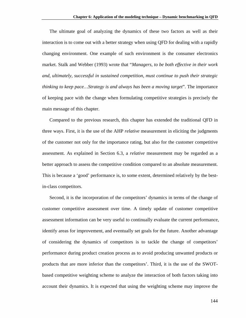
Chapter 6: Application of the modeling technique – Dynamic benchmarking in QFD
The ultimate goal of analyzing the dynamics of these two factors as well as their
interaction is to come out with a better strategy when using QFD for dealing with a rapidly
changing environment. One example of such environment is the consumer electronics
market. Stalk and Webber (1993) wrote that “Managers, to be both effective in their work
and, ultimately, successful in sustained competition, must continue to push their strategic
thinking to keep pace…Strategy is and always has been a moving target”. The importance
of keeping pace with the change when formulating competitive strategies is precisely the
main message of this chapter.
Compared to the previous research, this chapter has extended the traditional QFD in
three ways. First, it is the use of the AHP relative measurement in eliciting the judgments
of the customer not only for the importance rating, but also for the customer competitive
assessment. As explained in Section 6.3, a relative measurement may be regarded as a
better approach to assess the competitive condition compared to an absolute measurement.
This is because a ‘good’ performance is, to some extent, determined relatively by the best-
in-class competitors.
Second, it is the incorporation of the competitors’ dynamics in terms of the change of
customer competitive assessment over time. A timely update of customer competitive
assessment information can be very useful to continually evaluate the current performance,
identify areas for improvement, and eventually set goals for the future. Another advantage
of considering the dynamics of competitors is to tackle the change of competitors’
performance during product creation process as to avoid producing unwanted products or
products that are more inferior than the competitors’. Third, it is the use of the SWOT-
based competitive weighting scheme to analyze the interaction of both factors taking into
account their dynamics. It is expected that using the weighting scheme may improve the
144

Chapter 6: Application of the modeling technique – Dynamic benchmarking in QFD
145
accuracy of the final DQ’s priority, which in the end may hopefully increase the likelihood
of success of a product design or upgrade process.
The limitation of the proposed methodology is that it might take a certain amount of
time and efforts to collect the necessary data over time. However, it might be justified
considering the improved accuracy of the QFD’s results. It is worth noting that the data
collection should be carried out in a specific customer segment. For future research, a case
study to showcase the effectiveness of the proposed methodology is certainly of great
value. One potential extension is to apply the approach in developing innovative products
using QFD (Miguel, 2007).
In the next chapter (Chapter 7), a closer look at how the final DQs’ priorities, either
those obtained in this chapter or in Chapter 5, be translated into QCs’ priorities through
the QFD’s relationship matrix is provided. Specifically, the need to use normalization in
the relationship matrix will be thoroughly investigated. Afterwards, the decision making
issues based on the QCs’ priorities will be discussed in Chapter 8.

Chapter 7: A further study on QFD’s relationship matrix: Investigating the need of normalization
CHAPTER 7
A FURTHER STUDY ON QFD’S RELATIONSHIP MATRIX:
INVESTIGATING THE NEED OF NORMALIZATION
The last two chapters (Chapter 5 and 6) have shown the applications of the proposed new
modeling technique (Chapter 4). Both of the applications end with enhanced analysis of
the DQs via improving their priorities’ accuracy. After obtaining better DQs’ priorities,
the next step is to translate those DQs into QCs and finally obtain QCs’ priorities. Almost
all translations employ the so-called relationship matrix, which shows the strength of
relationship between the DQs and the QCs. The purpose of this chapter is to provide a
further study on the relationship matrix by investigating the need of normalizing it. It will
be shown that that either using or ignoring normalization, any QFD practitioner may still
be subject to misleading results. This therefore implies that normalization is not a trivial
issue. Through empirical examples, this chapter provides some guidelines for QFD
practitioners to decide when normalization is (not) necessary, especially when it causes
rank reversal. This chapter is reproduced from “On Normalizing the Relationship Matrix
in Quality Function Deployment”, by Raharjo H, Xie M, Brombacher AC. To be
submitted to an international journal.
7.1 Introduction
The most important function of QFD is to translate DQs into QCs (Chan and Wu,
2002a; Xie et al., 2003). How one DQ gets translated into one or more QCs may vary
from one case to another, and this is beyond the scope of this thesis. Nevertheless, almost
all translations do employ the so-called relationship matrix, which shows the strength of
146

Chapter 7: A further study on QFD’s relationship matrix: Investigating the need of normalization
relationship between the DQs and the QCs. It is this relationship matrix that becomes the
focal point of this chapter. It is of critical importance because it determines, together with
the DQs’ priorities, the final output of the house of quality, that is, the QCs’ priorities.
To obtain a more meaningful interpretation, some researchers suggest the use of
normalization in the relationship matrix. The most popular normalization technique in the
literature is the one proposed by Wasserman (Wasserman, 1993)1. Unfortunately, such
normalization also comes with some serious shortcomings (see Section 7.2). On the other
hand, there are also many other QFD researchers that do not use normalization or simply
ignore it. It is probably because most of them are not aware of the potential risk of having
misleading results. In other words, either using or ignoring normalization, any QFD
practitioner may still be subject to misleading results. This therefore implies that
normalization is not a trivial issue.
Unfortunately, there appears to have been almost no study that adequately addresses
this relationship matrix normalization issue in QFD at the moment. Therefore, this chapter
attempts to fill in this niche by providing a more detailed and fair explanation on the
relationship matrix normalization issue in QFD, particularly when it causes rank reversal.
In Section 7.3.1, it will be shown that the rank reversal, as a result of normalization, is
desirable. However, in Section 7.3.2, it will be shown otherwise. An empirical rule of
thumb for QFD practitioners to know whether normalization may lead to desirable results
is proposed in Section 7.4. It is especially useful when the size of the house of quality gets
larger. Finally, Section 7.5 concludes and provides possible extensions for future research.
1 According to Science Citation Index database, it has received 99 times citations as per May, 2009
147

Chapter 7: A further study on QFD’s relationship matrix: Investigating the need of normalization
It is expected that this work will eventually provide important information for any QFD
practitioner when dealing with the relationship matrix.
7.2. The QFD relationship matrix: some problems and research gap
7.2.1 Some problems in QFD relationship matrix
The relationship matrix is basically used for showing the relationship between the DQs
and the QCs. Traditionally, the relationship matrix employs a scale of ‘1-3-9’ to represent
the strength of association or relation between a certain DQ and a QC (Akao, 1990; Xie et
al., 2003). There have been some debates on the use of this scale. Two worth noting
problems that arise are whether this scale is mathematically sound and why not choosing
other scales, such as, ‘1-3-5’ or else.
The latter problem (scales selection) seems to be not really critical. A QFD practitioner
may basically select a scale that best represents their judgments. With respect to this,
Ghiya et al. (1999) carried out some experiments to test the robustness of the QFD results
when the traditional scale (‘1-3-9’) is replaced by others. Following the most common
practice, a scale of ‘1-3-9’ is used in this chapter.
On the other hand, the former problem (mathematical soundness), is of critical
importance. The underlying question is whether the scale, for example, ‘1-3-9’ belongs to
ordinal, interval, or ratio scale (Stevens, 1946). Otto of Massachusetts Institute of
Technology (Otto, 1995) showed that the QFD relationship matrix operates with ratio
scales. The reason is because it uses a zero value to anchor the scale. The zero value,
which is shown by a blank relationship, simply says that the technical attribute (QC) does
nothing to the customer need (DQ).
148

Chapter 7: A further study on QFD’s relationship matrix: Investigating the need of normalization
In this chapter, the above mathematical soundness problem is useful to preempt the
possibility to surmise that the normalization problem is caused by the types of scale, that
is, ordinal, interval, or ratio. In other words, the problem with normalization still exists
even though a ratio scale, which is the highest type of scale (Stevens, 1946), is assumed or
used.
It is worth highlighting that a ratio scale will be assumed throughout this thesis since it
is the only scale that may make the analysis meaningful. Some basic consequences when
using ratio scale for the scoring system of the relationship matrix, such as, the score can be
any real number from ‘0’ to ‘9’, ‘9’ is three times more correlated than ‘3’, ‘3’ is three
times more correlated than ‘1’, and so on (Burke et al., 2002) are also assumed.
7.2.2 The research gap
As mentioned previously, the most popular normalization method for the QFD
relationship matrix is the one proposed by Wasserman (Wasserman, 1993). Assuming that
there are m DQs and n QCs, the mathematical expression to normalize the relationship
values between the i-th DQ and the j-th QC (Rij) according to Wasserman is as follows:
∑∑
∑
= =
== n
j
n
kjkij
n
kkjik
normij
R
RR
1 1
1
.
.
γ
γ, i =1, 2,…, m; j =1, 2, …, n (7.1)
where:
normijR : the normalized relationship values between the i-th DQ and the j-th QC.
jkγ : the value to denote the degree of correlation between the j-th QC and the k-th QC
and vice versa (symmetrical). This value is shown in the roof of the HoQ.
149

Chapter 7: A further study on QFD’s relationship matrix: Investigating the need of normalization
Note that the value of jkγ is not normalized so that the highest value of the correlation is 9.
The value of the can be interpreted as the incremental change in the level of
fulfillment of the i-th DQ when the j-th QC is fulfilled to a certain level.
normijR
When the correlation between the QCs ( jkγ ) is assumed to be non-existent, then the
above formula can be reduced to a simple row normalization procedure as follows:
∑=
=n
jijij
normij RRR
1/ (7.2)
The final priorities of the QCs can be computed by taking the product of and IRi , as
expressed in formula (7.3).
normijR
∑=
=m
ii
normijj IRRAS
1. , i =1, 2,…, m; j =1, 2,…, n (7.3)
where:
ASj = Absolute Score of QCj
IRi = Importance Rating of DQi or DQi’s priority
Those final priorities, either in terms of absolute or relative scores, are of critical
importance to the QFD practitioners because they determine all subsequent decisions and
processes. For example, suppose there are four houses of quality used. Then, if there is
inaccuracy in the first house, then the error would certainly be propagated into the second,
third, and fourth houses. In other words, the entire product creation process will go wrong.
As a result, not only will it incur unnecessarily huge cost, but it will also result in
producing unwanted products.
150
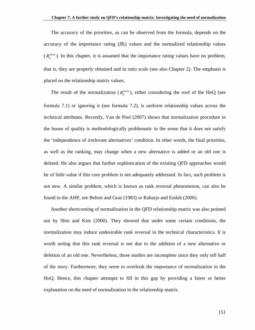
Chapter 7: A further study on QFD’s relationship matrix: Investigating the need of normalization
The accuracy of the priorities, as can be observed from the formula, depends on the
accuracy of the importance rating (IRi) values and the normalized relationship values
( ). In this chapter, it is assumed that the importance rating values have no problem,
that is, they are properly obtained and in ratio scale (see also Chapter 2). The emphasis is
placed on the relationship matrix values.
normijR
The result of the normalization ( ), either considering the roof of the HoQ (see
formula 7.1) or ignoring it (see formula 7.2), is uniform relationship values across the
technical attributes. Recently, Van de Poel (2007) shows that normalization procedure in
the house of quality is methodologically problematic in the sense that it does not satisfy
the ‘independence of irrelevant alternatives’ condition. In other words, the final priorities,
as well as the ranking, may change when a new alternative is added or an old one is
deleted. He also argues that further sophistication of the existing QFD approaches would
be of little value if this core problem is not adequately addressed. In fact, such problem is
not new. A similar problem, which is known as rank reversal phenomenon, can also be
found in the AHP, see Belton and Gear (1983) or Raharjo and Endah (2006).
normijR
Another shortcoming of normalization in the QFD relationship matrix was also pointed
out by Shin and Kim (2000). They showed that under some certain conditions, the
normalization may induce undesirable rank reversal in the technical characteristics. It is
worth noting that this rank reversal is not due to the addition of a new alternative or
deletion of an old one. Nevertheless, those studies are incomplete since they only tell half
of the story. Furthermore, they seem to overlook the importance of normalization in the
HoQ. Hence, this chapter attempts to fill in this gap by providing a fairer or better
explanation on the need of normalization in the relationship matrix.
151

Chapter 7: A further study on QFD’s relationship matrix: Investigating the need of normalization
7.3. The pros and cons of normalization in QFD
7.3.1 The pros
There are at least two reasons why normalization is desirable to be carried out in a
QFD analysis. First, it is to have a proportional demanded weight of the customer needs
(DQs), see Wasserman (1993) for details. In this chapter, it is represented by ‘RW’ (row
weight), and its relative value is represented by ‘RRW’ (relative row weight). Note that
the ‘RW’ is obtained from multiplying the importance rating (IR) by the sum of
relationship values in one row. Second, it is to avoid a misleading prioritization result.
This second point may be a novel case which has not been exposed in the existing
literature.
Below is an example of such case. Before normalization, the HoQ example in Table
7.1 gives counter intuitive results as follows. Note that ‘RS’ is used to denote the relative
score of the absolute score of QCj (ASj, see formula 7.3).
Table 7.1 HoQ example when normalization is desirable: before normalization
IR QC1 QC2 QC3 QC4 RW RRW
DQ1 0.1 9 1 3 9 2.2 0.42
DQ2 0.8 0 1 1 0 1.6 0.30
DQ3 0.1 3 3 0 9 1.5 0.281.2 1.2 1.1 1.8
0.23 0.23 0.21 0.342 2 4 1
ASRSRank
1. QC4 has the highest priority. This is clearly misleading because it has no relationship
with the most important customer need (DQ2), which has importance rating (IR) value
of 0.8.
152
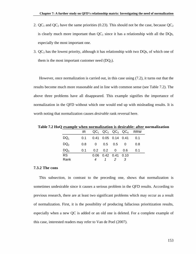
Chapter 7: A further study on QFD’s relationship matrix: Investigating the need of normalization
2. QC1 and QC2 have the same priorities (0.23). This should not be the case, because QC2
is clearly much more important than QC1 since it has a relationship with all the DQs,
especially the most important one.
3. QC3 has the lowest priority, although it has relationship with two DQs, of which one of
them is the most important customer need (DQ2).
However, once normalization is carried out, in this case using (7.2), it turns out that the
results become much more reasonable and in line with common sense (see Table 7.2). The
above three problems have all disappeared. This example signifies the importance of
normalization in the QFD without which one would end up with misleading results. It is
worth noting that normalization causes desirable rank reversal here.
Table 7.2 HoQ example when normalization is desirable: after normalization
IR QC1 QC2 QC3 QC4 RRW
DQ1 0.1 0.41 0.05 0.14 0.41 0.1
DQ2 0.8 0 0.5 0.5 0 0.8
DQ3 0.1 0.2 0.2 0 0.6 0.10.06 0.42 0.41 0.10
4 1 2 3RSRank
7.3.2 The cons
This subsection, in contrast to the preceding one, shows that normalization is
sometimes undesirable since it causes a serious problem in the QFD results. According to
previous research, there are at least two significant problems which may occur as a result
of normalization. First, it is the possibility of producing fallacious prioritization results,
especially when a new QC is added or an old one is deleted. For a complete example of
this case, interested readers may refer to Van de Poel (2007).
153

Chapter 7: A further study on QFD’s relationship matrix: Investigating the need of normalization
Second, it is the possibility of undesirable rank reversal due to normalization (Shin
and Kim, 2000). However, the reason of why it occurs was not adequately explained. The
following example demonstrates such situation, in which normalization does lead to
misleading results. In Table 7.3, it is clear that QC2 is the most important one since it has a
strong relationship with DQ1 (IR1=0.3) and a moderate relationship with DQ4 (IR4=0.2).
Furthermore, it is also obviously much more important than QC3.
Table 7.3 HoQ example when normalization is undesirable: before normalization
IR QC1 QC2 QC3 RW RRW
DQ1 0.3 3 9 0 3.6 0.49
DQ2 0.3 0 0 3 0.9 0.12
DQ3 0.2 1 0 1 0.4 0.05
DQ4 0.2 9 3 0 2.4 0.332.9 3.3 1.1
0.40 0.45 0.152 1 3
ASRSRank
However, once normalization is carried out using formula (7.2), the outcome (Table
7.4) shows an undesirable result. QC3, which was the least important, becomes the most
important one, while QC2, which was the most important, becomes the least important
one. It turns everything upside down. It is easy to see that QC2 is much more important
than QC3 because, with respect to the DQs which have importance rating value of 0.3 and
0.2, QC2 has three-time stronger relationships than QC3 does (see Table 7.3). For example,
with respect to the DQ which has an importance rating value of 0.3, QC3 has a ‘3’ (R23),
while QC2 has a ‘9’ (R12) which is three-time of ‘3’ (R12=3R23).
154

Chapter 7: A further study on QFD’s relationship matrix: Investigating the need of normalization
Table 7.4 HoQ example when normalization is undesirable: after normalization IR QC1 QC2 QC3 RRW
DQ1 0.3 0.25 0.75 0 0.3
DQ2 0.3 0 0 1 0.3
DQ3 0.2 0.5 0 0.5 0.2
DQ4 0.2 0.75 0.25 0 0.20.33 0.28 0.40
2 3 1RSRank
7.4 Some observations and a proposed rule of thumb
Having observed the two cases above, one might naturally ask whether normalization
in the relationship matrix is really necessary in QFD. In Section 7.3.1, it is shown that
normalization should be done to obtain reliable results, while in Section 7.3.2, it is shown
otherwise. There appears to be a possible confusion here, but ignorance is definitely not
bliss in this respect.
7.4.1 Some observations
If one takes a closer look at the two examples above, one might find at least two
general facts. First, normalization may change the final relative scores of the QCs. Second,
normalization may induce rank reversal when the magnitude of change is relatively high.
As shown in the two illustrative examples, the change may be (un)desirable.
Before going further to discuss how one can know whether a change is desirable or
not, it is useful to first know why the change, which may cause rank reversal, happens.
The main reason why it happens is that normalization converts the absolute values of the
number into relative values. Such conversion can possibly make some numbers, which are
low in terms of their absolute values, have much higher magnitude in terms of their
relative values. It is precisely this condition that causes rank reversal in the two illustrative
155

Chapter 7: A further study on QFD’s relationship matrix: Investigating the need of normalization
examples in Section 7.3. In other words, rank reversal may happen when there are
relatively few and weak relationships between DQs and QCs in a row. For example, if
there are only two ‘1’s (‘1’=weak relationship) in a row, then they will be changed into
two ‘0.5’s after normalization.
Now, the next issue is how one can know that rank reversal, as a result of
normalization, is desirable or not. By observing the two illustrative examples, the
following empirical analysis can be made:
1. It may be desirable when a very important customer need is weakly related to a
few technical attributes.
2. It may be undesirable when some relatively not very important customer needs are
weakly related to a few technical attributes.
For the first situation, which is exemplified in Section 7.3.1, the rank reversal is desirable
because it helps avoid the problem of ‘under’ translating the very important customer
need, see the row of DQ2 (Table 7.1 and Table 7.2). While for the second situation, which
is exemplified in Section 7.3.2, the rank reversal is undesirable because it causes ‘over’
translation of the relatively not very important needs, see the row of DQ2 and DQ3 (Table
7.3 and Table 7.4).
The above observations can be easily made since the size of the matrix is relatively
small. However, in most of the cases, the size of a QFD relationship matrix is relatively
large. This means that reliance on manual observation is at stake. Therefore, a kind of
guideline or rule of thumb would be very useful for QFD practitioners to decide whether
they need normalization or not. In the next subsection (Section 7.4.2), a guideline, which
may serve as the rule of thumb, will be proposed. Afterwards, a real-world QFD example
will be used to validate the proposed guideline (Section 7.4.3).
156

Chapter 7: A further study on QFD’s relationship matrix: Investigating the need of normalization
7.4.2 A proposed rule of thumb
The following guideline is proposed as a rule of thumb for QFD practitioners to decide
whether they need normalization in the relationship matrix.
Step 1. Normalize the relationship matrix using formula (7.1).
Step 2. Check if there is a significant2 change in the final relative scores of the QCs after
normalization. If there is, then proceed to the next step, otherwise, go to Step 4.
Note that rank reversal may occur when there are one or more big3 differences
between the RRWi and the IRi. The larger the matrix size, the more number of
big differences is required for a rank reversal to occur.
Step 3. Check if the change is desirable or not by comparing the relative row weight
(RRWi) and importance rating value (IRi) of each DQ. The change may be
desirable when those DQs which have low4 RRW values have one or more
relatively high IR values. Otherwise, it may be undesirable, that is, when those
DQs which have low RRW values have one or more relatively low IR values. In
the case when it is undesirable, the normalized matrix should not be used.
Step 4. Sanity check.
The rationale behind the proposed rule of thumb is described as follows. To judge
whether normalization may lead to desirable results, it is first necessary to compare the
results before and after normalization (Step 1). There are two possible outcomes, namely,
they are significantly different or not. If the results before and after normalization are not
2 A ‘significant’ change may be interpreted as a change that causes rank reversal. 3 A ‘big’ difference is defined as a difference of more than two-time higher or less than half-time lower than the value. 4 Pareto diagram can be used to classify those RRW which have ‘low’ values, for example, using the reciprocal value of RRW.
157

Chapter 7: A further study on QFD’s relationship matrix: Investigating the need of normalization
significantly different, then the use of normalization is optional. For the sake of simplicity,
a ‘significant’ change can be interpreted as a change that causes rank reversal (Step 2). It
is possible that there might be a significant change that does not necessarily cause rank
reversal. However, the investigation of such condition is beyond the scope of this thesis.
As the rule of thumb, it may be said that rank reversal may occur when there are one or
more big differences between the RRWi and the IRi. The reason why it suggests for more
than one big difference is because the RRW is a relative value. In other words, when one
RRW value becomes very small (less than half lower) in comparison with the IR value,
then this will most likely cause at least one other RRW value to become relatively higher
in comparison with the corresponding IR value.
If there is a rank reversal, then the next step is to indicate whether it is desirable or not
(Step 3). A more objective way to do this is by comparing the relative row weight (RRWi)
and importance rating value (IRi) of each DQ using the following rule of thumb:
1. It may be desirable when those DQs which have low RRW values have one or
more relatively high IR values. This is because normalization helps avoid the
problem of under-translating very important DQs, namely, those DQs which have
high IR values. If the relationship matrix is not normalized, then the values of
those very important DQs will tend to diminish when multiplied by the low
relationship value.
2. It may be undesirable when those DQs which have low RRW values have one or
more relatively low IR values. This is because normalization causes the problem of
over-translating the relatively not very important DQs, namely, those DQs which
have low IR values. If the relationship matrix is normalized, then the values of
those relatively not important DQs will tend to inflate when multiplied by the
158

Chapter 7: A further study on QFD’s relationship matrix: Investigating the need of normalization
normalized relationship value.
This guideline can be regarded as a way to verify the proposed rule of thumb and to decide
whether normalization is really needed in the QFD relationship matrix. It is worth
highlighting that the above proposed rule of thumb can also be applied to verify the two
illustrative examples in Section 7.3. Finally, a sanity check can be carried out before
subsequent downstream analysis.
7.4.3 A validation example
A recent real-world QFD application, which is published in a reputable journal (Sireli
et al., 2007), was taken as a case study to validate how the proposed rule of thumb may
work in practice. Two houses of quality of quite large size were adopted for the purpose of
illustrating how QFD practitioners may decide whether normalization is necessary or not.
For the first HoQ example, it was taken from page 388 of the paper (Sireli et al.,
2007), under the heading ‘Combined Model for the Basic Product’. For the sake of
simplicity, the DQs’ and QCs’ detailed names are not included.
Step 1: Normalize the relationship matrix using formula (7.1). Since the correlation
matrix is non-existent, formula (7.2) can be used to normalize the relationship matrix. The
original and the normalized HoQ can be seen in Table 7.5 and Table 7.6, respectively.
Step 2: Check if there is a significant change in the final relative scores of the QCs
after normalization. It is easy to see that there is a rank reversal after normalization. The
fourth and the fifth ranks are reversed. It is also interesting to see that the rank reversal
happens because there are more than one big difference between the RRWi and the IRi, as
precisely prescribed in the rule of thumb.
159
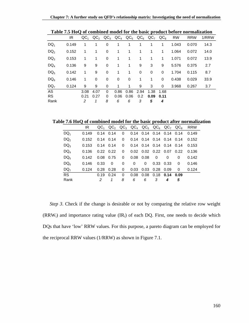
Chapter 7: A further study on QFD’s relationship matrix: Investigating the need of normalization
Table 7.5 HoQ of combined model for the basic product before normalization IR QC1 QC2 QC3 QC4 QC5 QC6 QC7 QC8 RW RRW 1/RRW
DQ1 0.149 1 1 0 1 1 1 1 1 1.043 0.070 14.3
DQ2 0.152 1 1 0 1 1 1 1 1 1.064 0.072 14.0
DQ3 0.153 1 1 0 1 1 1 1 1 1.071 0.072 13.9
DQ4 0.136 9 9 0 1 1 9 3 9 5.576 0.375 2.7
DQ5 0.142 1 9 0 1 1 0 0 0 1.704 0.115 8.7
DQ6 0.146 1 0 0 0 0 1 1 0 0.438 0.029 33.9
DQ7 0.124 9 9 0 1 1 9 3 0 3.968 0.267 3.73.08 4.07 0 0.86 0.86 2.94 1.38 1.680.21 0.27 0 0.06 0.06 0.2 0.09 0.11
2 1 8 6 6 3 5 4
ASRSRank
Table 7.6 HoQ of combined model for the basic product after normalization IR QC1 QC2 QC3 QC4 QC5 QC6 QC7 QC8 RRW
DQ1 0.149 0.14 0.14 0 0.14 0.14 0.14 0.14 0.14 0.149DQ2 0.152 0.14 0.14 0 0.14 0.14 0.14 0.14 0.14 0.152DQ3 0.153 0.14 0.14 0 0.14 0.14 0.14 0.14 0.14 0.153DQ4 0.136 0.22 0.22 0 0.02 0.02 0.22 0.07 0.22 0.136DQ5 0.142 0.08 0.75 0 0.08 0.08 0 0 0 0.142DQ6 0.146 0.33 0 0 0 0 0.33 0.33 0 0.146DQ7 0.124 0.28 0.28 0 0.03 0.03 0.28 0.09 0 0.124
0.19 0.24 0 0.08 0.08 0.18 0.14 0.092 1 8 6 6 3 4 5
RSRank
Step 3. Check if the change is desirable or not by comparing the relative row weight
(RRWi) and importance rating value (IRi) of each DQ. First, one needs to decide which
DQs that have ‘low’ RRW values. For this purpose, a pareto diagram can be employed for
the reciprocal RRW values (1/RRW) as shown in Figure 7.1.
160

Chapter 7: A further study on QFD’s relationship matrix: Investigating the need of normalization
1/RRW 33.94 14.25 13.97 13.88 8.72 3.75 2.67Percent 37.2 15.6 15.3 15.2 9.6 4.1 2.9Cum % 37.2 52.9 68.2 83.4 93.0 97.1 100.0
DQs OtherDQ7DQ5DQ3DQ2DQ1DQ6
90
80
70
60
50
40
30
20
10
0
100
80
60
40
20
0
1/RR
W
Perc
ent
Pareto Chart of Combined Model for the Basic Product
Figure 7.1 Pareto chart of combined model for the basic product
It can be seen that DQ1, DQ2, DQ3, and DQ6 may belong to the DQ group which have low
RRW values. Since DQ6 corresponds to a quite high IR value (IR6= 14.6%) and DQ3
corresponds to the highest IR value (IR3=15.3%), then it is clear that the rank reversal is
desirable. In other words, the normalization is necessary to be carried out. Finally, a sanity
check (Step 4) can be done for subsequent analysis.
For the second HoQ example, it was also taken from page 388 of the paper (Sireli et
al., 2007), under the heading ‘Combined Model for the High-End Product’. For the sake of
simplicity, the DQs’ and QCs’ detailed names are again not included.
Step 1: Normalize the relationship matrix using formula (1). Since the correlation
matrix is non-existent, formula (2) can again be used to normalize the relationship matrix.
The original and the normalized HoQ can be seen in Table 7.7 and Table 7.8, respectively.
Step 2: Check if there is a significant change in the final relative scores of the QCs
after normalization. It is easy to see that there is a rank reversal after normalization. The
rank of QC2 and QC3 are reversed. Initially, QC3 has a higher rank than QC2, but it is the
other way around after normalization. It is again confirmed that what is prescribed in the
161

Chapter 7: A further study on QFD’s relationship matrix: Investigating the need of normalization
rule of thumb is correct, that is, the rank reversal happens because there are more than one
big difference between the RRWi and the IRi.
Table 7.7 HoQ of combined model for the high-end product before normalization
IR QC1 QC2 QC3 QC4 QC5 QC6 QC7 QC8 RRW
DQ1 0.073 0.19 0.02 0.00 0.19 0.02 0.19 0.19 0.19 0.073
DQ2 0.066 0.19 0.02 0.00 0.19 0.02 0.19 0.19 0.19 0.066
DQ3 0.070 0.19 0.02 0.00 0.19 0.02 0.19 0.19 0.19 0.070
DQ4 0.077 0.19 0.02 0.00 0.19 0.02 0.19 0.19 0.19 0.077
DQ5 0.081 0.19 0.02 0.00 0.19 0.02 0.19 0.19 0.19 0.081
DQ6 0.049 0.20 0.00 0.00 0.20 0.20 0.20 0.20 0.00 0.049
DQ7 0.067 0.24 0.03 0.00 0.08 0.08 0.24 0.24 0.08 0.067
DQ8 0.080 0.19 0.19 0.00 0.02 0.02 0.19 0.19 0.19 0.080
DQ9 0.098 0.50 0.00 0.00 0.00 0.00 0.50 0.00 0.00 0.098
DQ10 0.075 0.50 0.00 0.00 0.00 0.00 0.50 0.00 0.00 0.075
DQ11 0.065 0.50 0.00 0.00 0.00 0.00 0.50 0.00 0.00 0.065
DQ12 0.068 0.50 0.00 0.00 0.00 0.00 0.50 0.00 0.00 0.068
DQ13 0.061 0.50 0.00 0.00 0.00 0.00 0.50 0.00 0.00 0.061
DQ14 0.071 0.00 0.00 1.00 0.00 0.00 0.00 0.00 0.00 0.0710.295 0.025 0.071 0.087 0.025 0.295 0.112 0.091
1 7 6 5 7 1 3 4RSRank
Table 7.8 HoQ of combined model for the high-end product after normalization IR QC1 QC2 QC3 QC4 QC5 QC6 QC7 QC8 RW RRW 1/RRW
DQ1 0.073 9 1 0 9 1 9 9 9 3.431 0.111 9.03
DQ2 0.066 9 1 0 9 1 9 9 9 3.102 0.100 9.99
DQ3 0.070 9 1 0 9 1 9 9 9 3.29 0.106 9.42
DQ4 0.077 9 1 0 9 1 9 9 9 3.619 0.117 8.56
DQ5 0.081 9 1 0 9 1 9 9 9 3.807 0.123 8.14
DQ6 0.049 1 0 0 1 1 1 1 0 0.245 0.008 126.4
DQ7 0.067 9 1 0 3 3 9 9 3 2.479 0.080 12.5
DQ8 0.080 9 9 0 1 1 9 9 9 3.76 0.121 8.24
DQ9 0.098 9 0 0 0 0 9 0 0 1.764 0.057 17.5
DQ10 0.075 9 0 0 0 0 9 0 0 1.35 0.044 22.9
DQ11 0.065 9 0 0 0 0 9 0 0 1.17 0.038 26.4
DQ12 0.068 9 0 0 0 0 9 0 0 1.224 0.040 25.3
DQ13 0.061 9 0 0 0 0 9 0 0 1.098 0.035 28.2
DQ14 0.071 0 0 9 0 0 0 0 0 0.639 0.021 48.47.978 1.154 0.639 3.633 0.697 7.978 4.675 4.2240.258 0.037 0.021 0.117 0.022 0.258 0.151 0.136
1 6 8 5 7 1 3 4
ASRSRank
4
0
6
5
8
1
1
8
162
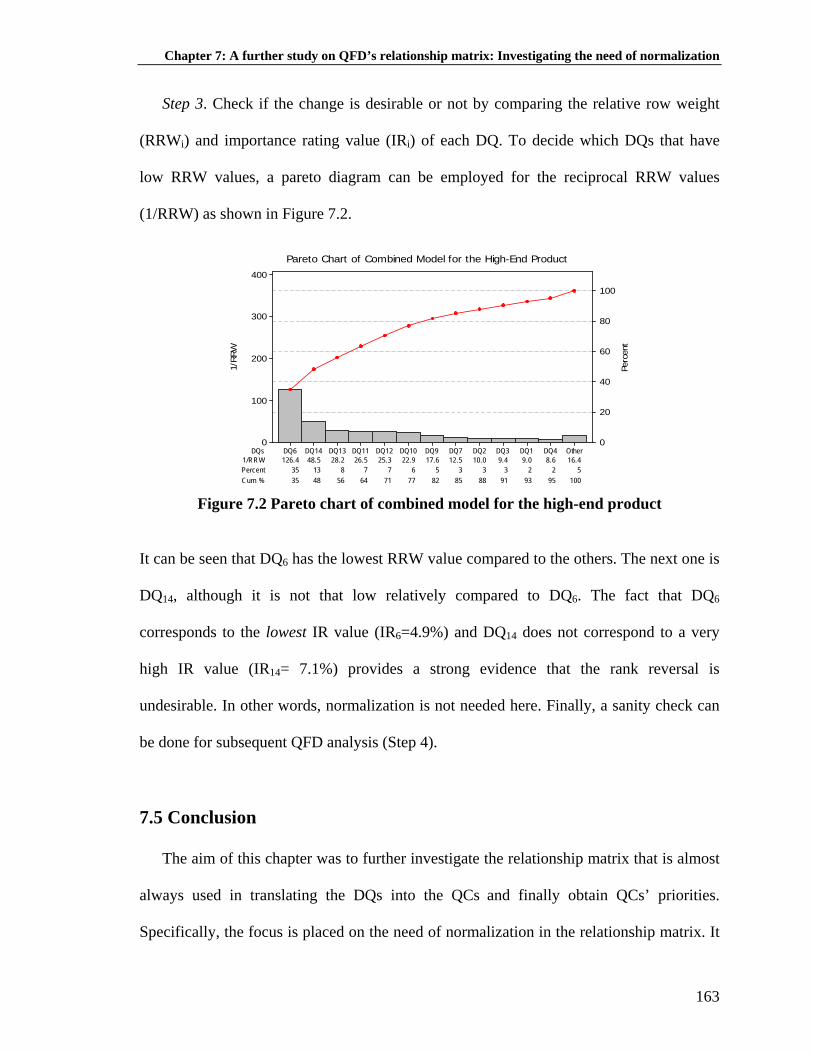
Chapter 7: A further study on QFD’s relationship matrix: Investigating the need of normalization
Step 3. Check if the change is desirable or not by comparing the relative row weight
(RRWi) and importance rating value (IRi) of each DQ. To decide which DQs that have
low RRW values, a pareto diagram can be employed for the reciprocal RRW values
(1/RRW) as shown in Figure 7.2.
1/RRW 10.0 9.4 9.0 8.6 16.4126.4 48.5 28.2 26.5 25.3 22.9 17.6 12.5Percent 3 3 2 2 535 13 8 7 7 6 5 3Cum % 88 91 93 95 10035 48 56 64 71 77 82 85
DQs OtherDQ4DQ1DQ3DQ2DQ7DQ9DQ10DQ12DQ11DQ13DQ14DQ6
400
300
200
100
0
100
80
60
40
20
0
1/RR
W
Perc
ent
Pareto Chart of Combined Model for the High-End Product
Figure 7.2 Pareto chart of combined model for the high-end product
It can be seen that DQ6 has the lowest RRW value compared to the others. The next one is
DQ14, although it is not that low relatively compared to DQ6. The fact that DQ6
corresponds to the lowest IR value (IR6=4.9%) and DQ14 does not correspond to a very
high IR value (IR14= 7.1%) provides a strong evidence that the rank reversal is
undesirable. In other words, normalization is not needed here. Finally, a sanity check can
be done for subsequent QFD analysis (Step 4).
7.5 Conclusion
The aim of this chapter was to further investigate the relationship matrix that is almost
always used in translating the DQs into the QCs and finally obtain QCs’ priorities.
Specifically, the focus is placed on the need of normalization in the relationship matrix. It
163

Chapter 7: A further study on QFD’s relationship matrix: Investigating the need of normalization
is hoped that the work in this chapter will provide a better or fairer explanation on the
need of normalization in the QFD relationship matrix, especially when it causes rank
reversal. The existing literature, as has been described, does not provide adequate
information on this issue. Some researchers might say that it is necessary to carry out
normalization to have more meaningful results, while some others might say
normalization make things worse by opening up the possibility of rank reversal when one
technical attribute is added or deleted. Still, some others might not bother about this.
Probably, it is regarded as a non-added value step in the HoQ.
This chapter has shown that, in all cases, any QFD practitioner should be aware that
normalization, in general, is not a trivial issue when dealing with the relationship matrix.
In particular, if the RRW value of the relationship matrix exhibits a special pattern as
described in this chapter, then it indicates that rank reversal may happen when
normalization is done. The question is whether such reversal is desirable or not. Based on
some empirical observations, a rule of thumb is proposed for any QFD practitioner to
know when such reversal may be desirable, that is, when normalization may lead to better
results.
Since the rule of thumb is based on an empirical basis, it might not work perfectly for
every single case, especially for large-sized HoQ. Hence, this opens up a new challenge
for future research to complement the current findings. Some approaches, such as,
computer simulations or validation by more real-world case studies might be considered.
For other possible future works, there are at least two clear directions to pursue. First, it
might be interesting to investigate how one can know, in the case of no rank reversal, that
the change due to normalization is (un)desirable. Second, the incorporation of fuzzy
theory to facilitate a more precise quantification of the words, such as ‘weak’, ‘few’,
164

Chapter 7: A further study on QFD’s relationship matrix: Investigating the need of normalization
165
‘high’, and so on might be a considerable option. In sum, it is expected that this work, as a
first step, will provide an important guideline or useful insights for QFD practitioners in
general when dealing with the relationship matrix.
In the next chapter (Chapter 8), taking into account the need of normalization
discussed thoroughly in this chapter, how the DQs’ priorities will be used to obtain QCs’
priorities and finally be used as the main input for decision making will be described. For
the decision making purpose, two kinds of approaches are suggested for prioritizing
and/or optimizing the QCs. The objective is to better meet the changing needs of the
customer considering the research problem discussed in Chapter 1.

Chapter 8: A further study on prioritizing quality characteristics in QFD
CHAPTER 8
A FURTHER STUDY ON PRIORITIZING QUALITY
CHARACTERISTICS IN QFD
The purpose of this chapter is to provide a possible answer to the research question “How
to make decision in a QFD analysis with respect to the dynamics in the house of quality?”
To the extent of what is described in the delimitation section, this chapter will answer the
question by proposing a methodology, which may use two kinds of decision making
approaches, to prioritize or optimize the QCs with respect to the dynamics in the HoQ.
The methodology employs the modeling technique proposed in Chapter 4 as the tool to
forecast the dynamics. To show how the methodology works in practice, the case study
described in Chapter 2 is used to provide the contextual setting. The notion of future
uncertainty to improve forecast’ precision will also be introduced. It is hoped that the
proposed methodology might help QFD-users better deal with the future needs of the
customer. A large part of this chapter is reproduced from the author’s two papers1.
8.1 Introduction
In the context of a customer-driven product or service design process, a timely update
of customer needs information may not only serve as a useful indicator to observe how
things change over time, but it also provides the company a better ground to formulate
strategies to meet the future needs of its customer. This chapter proposes a systematic
1 Raharjo, H., Xie, M., Brombacher, A.C. (2006), Prioritizing Quality Characteristics in Dynamic Quality Function Deployment, International Journal of Production Research, 44(23), 5005-5018. (received IJPR highly-commended PhD prize 2007)
Raharjo, H., Xie, M., Brombacher, A.C., A systematic methodology to deal with the dynamics of customer needs in Quality Function Deployment, Submitted to an international journal.
166

Chapter 8: A further study on prioritizing quality characteristics in QFD
methodology to better deal with customer needs’ dynamics, in terms of their relative
weights (priorities), in the QFD.
The work in this chapter will extend the existing QFD research in three directions.
First, it provides the way to model the change of relative priorities of the DQs over time.
This is owing to the fact that the AHP has been applied quite extensively in QFD (see
Chapter 1 and Chapter 2), and yet there has been almost no tool to model the dynamics.
Second, it proposes the notion of future uncertainty, which is an interval estimate of the
future needs, as a way to improve the forecast precision. This is to complement the
previous research which use only a point estimate of the future needs (Min and Kim,
2008; Raharjo et al., 2006; Wu and Shieh, 2006; Wu et al., 2005). Third, it proposes the
use two quantitative decision making approaches that take into account the decision
maker’s attitude towards risk in optimizing or prioritizing the QCs with respect to the
future needs of the customer.
This chapter is organized as follows. In the next section (Section 8.2), the notion of
dynamic QFD (DQFD) will be described in terms of its significance, model, and tools
used. Section 8.3 will elaborate the proposed systematic methodology to deal with the
customer needs’ dynamics along with their future uncertainty using two decision making
approaches. An example based on a real world application of QFD (Raharjo et al., 2007;
see Chapter 2) will be provided to illustrate how the proposed methodology works in
practice (Section 8.4). Section 8.5 will discuss the issue of forecasting technique’s
selection and a possible implication of the methodology to development of innovative
products. Finally, a summary of the main contributions and possible future works are
provided in Section 8.6.
167

Chapter 8: A further study on prioritizing quality characteristics in QFD
8.2 The dynamic QFD (DQFD)
This section describes the notion of dynamic QFD (DQFD) that can be considered as
an extension of the standard QFD (Cohen, 1995) since it takes into account the change
over time. The emphasis here is placed on the need to deal with the dynamics in the
relative weights of customer needs (DQs’ priorities) 2 . Those weights are commonly
referred to as ‘importance rating’ in the house of quality (HoQ). The following
subsections will first explain why it is important to consider such change. Afterwards,
how to quantitatively incorporate it in the HoQ along with its future uncertainty will be
elaborated.
8.2.1 Why is it important to incorporate customer needs’ dynamics?
QFD starts and ends with the customer. As explained in the research problem (Section
1.1), it is known that it always takes some time from the time when the customer voice is
collected until the time when the product is ready to be launched (see also Figure 1.1). The
time-lag duration may certainly vary from one product to another. For example, if it takes
one year time, then the question is whether the product which is about to be launched may
still meet the customer needs since it is created based on the customer voice which was
collected one year ago. The answer to this question is very likely to be a ‘no’ in the
context of today’s rapidly changing market.
Since the accuracy of information in the DQs critically determines the success of a
QFD application (Cristiano et al., 2001), it is of considerable importance to take into
account the change during product or service creation process. In Chapter 2 and Chapter 3,
2 The dynamics of DQs’ competitive assessment, as described in Chapter 6, may also be included in a similar way. For simplicity, only the dynamics in DQs’ priorities is included in the DQFD in this chapter
168
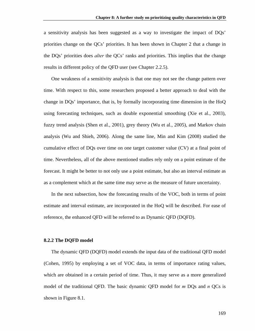
Chapter 8: A further study on prioritizing quality characteristics in QFD
a sensitivity analysis has been suggested as a way to investigate the impact of DQs’
priorities change on the QCs’ priorities. It has been shown in Chapter 2 that a change in
the DQs’ priorities does alter the QCs’ ranks and priorities. This implies that the change
results in different policy of the QFD user (see Chapter 2.2.5).
One weakness of a sensitivity analysis is that one may not see the change pattern over
time. With respect to this, some researchers proposed a better approach to deal with the
change in DQs’ importance, that is, by formally incorporating time dimension in the HoQ
using forecasting techniques, such as double exponential smoothing (Xie et al., 2003),
fuzzy trend analysis (Shen et al., 2001), grey theory (Wu et al., 2005), and Markov chain
analysis (Wu and Shieh, 2006). Along the same line, Min and Kim (2008) studied the
cumulative effect of DQs over time on one target customer value (CV) at a final point of
time. Nevertheless, all of the above mentioned studies rely only on a point estimate of the
forecast. It might be better to not only use a point estimate, but also an interval estimate as
as a complement which at the same time may serve as the measure of future uncertainty.
In the next subsection, how the forecasting results of the VOC, both in terms of point
estimate and interval estimate, are incorporated in the HoQ will be described. For ease of
reference, the enhanced QFD will be referred to as Dynamic QFD (DQFD).
8.2.2 The DQFD model
The dynamic QFD (DQFD) model extends the input data of the traditional QFD model
(Cohen, 1995) by employing a set of VOC data, in terms of importance rating values,
which are obtained in a certain period of time. Thus, it may serve as a more generalized
model of the traditional QFD. The basic dynamic QFD model for m DQs and n QCs is
shown in Figure 8.1.
169

Chapter 8: A further study on prioritizing quality characteristics in QFD
QC1 … …QC2 … …… … … … …
QCn … …
DQ QC QC
1
QC
2
… QC
n
Impo
rtanc
e ra
ting
(t=1
)
Impo
rtanc
e ra
ting
(t=2
)
…
Impo
rtanc
e R
atin
g (t
=k)
Fore
cast
ed IR
(t=k
+1)
Fore
cast
ing
Res
idua
l Std
Dev
(t
=k+1
)
DQ1 … IR1,1 IR1,2 … IR1,k IR1,k+1 Sd1
DQ2 … … IR2,1 … … IR2,k IR2,k+1 Sd2
… … … … … … … …
DQm … … IRm,1 … … IRm,k IRm,k+1 Sdm
Mean of forecasted QCj priority …
StDev of forecasted QCj priority …
… … …
VOC dynamics
nμ
1σ
2μ
nσ
12R nR1
21R
1mR mnR
11γ
nR2
n1γ
21γ
1nγ nnγ
n2γ
11R
1μ
2σ Figure 8.1 The DQFD model
It is quite common to first normalize the relationship matrix ( ), while considering
the correlation among the QCs, using the method proposed by Wasserman (1993). A
detailed discussion on the need of normalization in the relationship matrix is provided in
Chapter 7. The priorities of the QCs in the DQFD model can be computed by taking the
product of and the forecasted importance rating (IRi,k+1), as expressed in formula
(8.1) below.
ijR
normijR
∑=
+=m
iki
normijj IRR
11,.μ , i =1, 2,…, m; j =1, 2,…, n (8.1)
where
jμ = mean of forecasted priority of QCj
IRi,k+1 = forecasted importance rating of DQi or DQi’s priority.
k = last period of observation or number of observations
170

Chapter 8: A further study on prioritizing quality characteristics in QFD
Those QCs’ priorities are of critical importance to the QFD practitioners because they
determine all subsequent decisions and processes. One important idea in the DQFD is to
not only incorporate the forecasted point, but also the uncertainty measure (interval
estimate) of the forecast (see subsection 8.2.4 for more detailed explanation). In Figure
8.1, the future uncertainty of the forecasted importance rating is represented by the
standard deviation of the forecasting residual ( ). These values can be transmitted
into the standard deviation of QCj’s forecasted priority using the principle of variance
addition below:
iSd iSd
njRm
ii
normijj 2,...,1,,ˆ*ˆ
1
2 =∀= ∑=
σσ (8.2)
where jσ is the standard deviation of QCj’s forecasted priority and is the variance of
the forecasting residual of IRi or the squared value of . Note that such computation
may slightly reduce the value of the transmitted variance due to the multiplication of
normalized scores ( ).
2ˆ iσ
iSd
normijR
8.2.3 The forecasting technique
The purpose of using a forecasting technique in the DQFD is to model the change of
the importance rating values (DQs’ priorities) over time. The newly developed short-term
forecasting technique, namely, the CDES technique will be used to model the change of
DQs’ priorities over time. The details of the technique can be found in Chapter 4. An
important fact that should be noted with respect to the use of forecasting technique is that
a good forecasting method will ideally result in errors which follow a ‘Gaussian white
noise’ process, namely, a process which is normally, independently, identically distributed
171

Chapter 8: A further study on prioritizing quality characteristics in QFD
(NIID) with a zero mean value and a constant variance. In the next subsection, how the
information from the Gaussian white noise error may be used as an estimate of future
uncertainty of the forecasted importance rating will be elaborated.
8.2.4 Estimation of future uncertainty
The rationale of future uncertainty’s estimation is built upon the idea of how well one
may learn from the past experience, that is, how precisely one can model or learn from the
past data may critically determine how precisely one may estimate or understand the
future. On the ground of this reason, it is suggested that the future uncertainty be
estimated from the fitting imprecision of the forecasting model, which is represented by
the variance of the Gaussian white noise error.
For the proposed forecasting technique (Raharjo et al., 2009), the Aitchison distance
(Aitchison, 2003), which is a scalar quantity, is used as the primary yardstick to judge the
goodness of fit of the model. For a given time t, the measure of discrepancy between the
actual importance rating values (IR) and the fitted ones (IR') for DQi (i=1,…, m) is as
follows:
'( , ') ln ln( ) ( ')
ii
IR IRAd IR IRg IR g IR
⎛ ⎞= −⎜ ⎟⎝ ⎠
i , where 1
( )m
m ii
g IR IR=
= ∏ , 1
( ') 'm
m ii
g IR IR=
= ∏ (8.3)
Note that the sum of all the m IR values, for a given time t, is equal to 1 since they are
normalized, as a result of using the AHP. In the example section (Section 8.4), a full
residual analysis based on the properties of Gaussian white noise will be demonstrated.
After computing the forecasting residual, the forecasted points along with their
variances will be transmitted to the QCs’ priorities using formula (8.1) and (8.2). Since a
linear combination of several normal random variables is also normal, the forecasted QCs’
172

Chapter 8: A further study on prioritizing quality characteristics in QFD
priorities, which are shown in the last two rows of Figure 8.1, can be regarded as several
normally distributed processes with a mean value of jμ and a standard deviation value of
jσ . Thus, the problem is now how one may prioritize or optimize those QCs with respect
to their mean and standard deviation values. This problem will be discussed in the next
subsection.
8.2.5 Decision making
The general objective the decision making process is to meet the future needs of the
customer with greater confidence while considering the time lag problem (Section 1.1).
Two kinds of decision making models are suggested as the tools for prioritizing and/or
optimizing the QCs. One is based on a utilitarian approach, that is, using stochastic
dominance approach, and the other is based on a non-utilitarian approach, that is, using
Taguchi’s Quality Loss Function (QLF) approach and Zero One Goal Programming
(ZOGP).
In the utilitarian approach, the stochastic dominance (SD) approach (Hadar and Russel,
1974; Levy, 1998) is proposed to stochastically order the QCs. The stochastic ordering
results will become the basis to construct an SD constraint to be used in the optimization
model. The reason of choosing SD approach is two-fold. One is due to its simplicity and
theoretical rigor, and the other is its ability to consider the QFD team’s attitude towards
risk in making the decision. The SD approach does not require specific information of
decision maker’s utility function, but the result can still be consistent with the preference
of most decision makers (Hadar and Russel, 1974). In the QFD literature, the SD
technique has been suggested by Kim et al. (2007) to deal with the uncertainty which
173

Chapter 8: A further study on prioritizing quality characteristics in QFD
comes from ‘heterogeneity’ in customer’s perception. This chapter will provide a more
extensive application of the SD technique in QFD, especially in combination with the
optimization model.
With respect to the same problem, that is, to prioritize and/or optimize the QCs based
on their forecasted mean and standard deviation values, another equally plausible
approach, without considering decision maker’s attitude towards risk (non-utilitarian), can
be employed. The idea is to use the combination of Taguchi’s loss function approach and
the goal programming (Raharjo et al., 2006). The loss function approach is used to
minimize the deviation from the target mean and target variability. In other words, the
more it deviates away from the target value, the larger the loss will incur. The goal
programming is used to select only the ‘important’ QCs which have larger priorities and
lower variability while considering the decision maker’s preference.
It is worth noting that these two models can also be applied to the case when Kano’s
model is used to obtain the forecasted DQs’ priorities (Chapter 5) or when using the
competitive assessment of the DQs (Chapter 6). What is basically needed, as the main
input in the optimization models, is the forecasted DQs’ priorities and their future
uncertainty which is estimated from the variance of forecast residual. The next section
(Section 8.3) will describe how these two models can be used systematically within the
proposed methodology.
8.3 The proposed methodology
This section consists of three subsections. The first subsection (Section 8.3.1)
describes the proposed methodology. The methodology consists of 10 systematic steps
174

Chapter 8: A further study on prioritizing quality characteristics in QFD
which may employ two kinds of decision making approaches. The first six steps (Step 1 to
Step 6) are the common steps for using both approaches. They employ the same
forecasting technique (Raharjo et al., 2009; Chapter 4), the same way of estimating future
uncertainty, and the same way of obtaining the forecasted mean and standard deviation of
QCs’ priorities.
The next four steps are different; one may choose which decision making approach to
use. If the utilitarian approach is chosen, then follow the next four step indicated by ‘a’
(Step 7a to Step 10a). Otherwise, if the non-utilitarian approach is chosen, then follow the
next four step indicated by ‘b’ (Step 7b to Step 10b). Section 8.3.2 describes the utilitarian
approach, while Section 8.3.3 describes the non-utilitarian approach. Both decision
making approaches will be tested in the example section using the case study described in
Chapter 2 (Raharjo et al., 2007).
8.3.1 A step-by-step procedure
The objective of the proposed methodology is to provide a systematic approach to deal
with the dynamics of customer needs. A step-by-step procedure, starting from the
construction of the DQFD until the prioritization stage, is provided as follows. Note that,
as mentioned previously, the 10-step methodology comprised of six common steps and
four specific steps depending on which approach to use.
Step 1: Construct the HoQ using basic QFD steps, such as collecting customer needs using
in-depth interview or direct observation, structuring the needs using affinity
diagram, and finally prioritizing them using the AHP (Griffin and Hauser, 1993;
Cohen 1995: Raharjo et al., 2007).
175

Chapter 8: A further study on prioritizing quality characteristics in QFD
Step 2: Translate the DQs into appropriate QCs and fill up the elements in the house of
quality.
Step 3: Record the AHP-based importance rating values (DQs’ priorities) for k periods,
that is, IRi,t, IRi,t+1, IRi,t+2,…, IRi,k (see Figure 8.1, indicated as ‘VOC dynamics’).
Note that these IR values over time should be obtained from a specific segment of
customer.
Step 4: Fit the DQs’ priorities data change over time using the proposed forecasting
technique (Raharjo et al., 2009; Chapter 4), and obtain the future uncertainty’s
estimate, that is, the standard deviation of forecasting residual. If the forecasting
residual, which is obtained from equation (8.3), follows Gaussian white noise
process, then proceed to the next step. Otherwise, another forecasting technique is
called for (see Section 8.5.1).
Step 5: Obtain the forecasted IR (IRi,k+1) for each DQ using the forecasting method.
Step 6: Compute the mean and standard deviation of forecasted QCs’ priorities using
formula (8.1) and (8.2), respectively.
8.3.2 Optimization model 1: Utilitarian approach
Basically, the SD approach is comprised of some rules which are used to decide the
stochastic ordering of the alternatives being compared. The way to use those rules is to
start from the lowest order to a higher order. In the case when the lower order rule does
not give a conclusive solution, then a higher order rule is used. Having known those rules,
one can use them for ranking the QCs with respect to their mean and standard deviation
values.
176

Chapter 8: A further study on prioritizing quality characteristics in QFD
Step 7a: Plot the cumulative density function (CDF) of all QCs according their mean and
standard deviation values together in one graph. This step is very useful for
screening purpose because some QCs that obviously dominate the others can be
easily detected by visual inspection.
Step 8a: Check for first-order dominance using the CDF curves. The CDF curve will
reveal those QCs that first-order stochastically dominate the others. Specifically,
if QCa first-order dominates QCb, then the CDF of QCa is always to the right of
that of QCb. The assumption here is the larger the value of the QC, the more
important it becomes. In addition, if QCa first-order stochastically dominates QCb
(QCa QCb), then QCa also stochastically dominates QCb by second-degree,
third-degree, and so forth. However, the reverse is not true.
)1(f
Step 9a: Check if there is a crossing among the CDF curves. If so, then check for higher
order dominance, otherwise, proceed to the next step. In most cases, no more than
third-order dominance needs to be checked.
Step 10a: Stochastically order the QCs according to the dominance relationship result, and
construct a resource allocation constraint based on the stochastic ordering.
The stochastic ordering reflects the preference of the decision maker on the QCs. In
other words, a bigger portion of available resources should be allocated to those QCs that
dominate the others. Unfortunately, unlike the mean-variance method, the SD approach,
which considers the entire return distribution rather than selected moments, does not
provide a straightforward way for diversification purpose (Levy, 1998). Thus, it is not
177

Chapter 8: A further study on prioritizing quality characteristics in QFD
easy to decide precisely what percentage of the resources that should be allocated in the
stochastically ordered alternatives.
The stochastic ordering result is used as the basis for resource allocation in the sense
that it restricts the amount of resources which are allocated among the QCs. For example,
if there exists QCa o-order stochastically dominates QCb or , then the
amount of resource allocated to QCa should be higher than that of QCb. It can be
quantitatively expressed as
b(o)a QCQC f
δ≥− ba XX , where δ is the minimum amount of acceptable
difference between the allocated resource in QCa and QCb.
To show how the SD results can be applied in an optimization framework, a simple
customer satisfaction optimization model based on Xie et al (2003) is adopted. The
objective is to maximize the total customer satisfaction (Z) by optimizing the available
resources, for example, the allocated cost for each QC with respect to its target value. The
complete optimization model is given in (8.4)-(8.8). The SD result, namely, the stochastic
ordering of the QCs, is translated into equation (8.7). It is worth noting that the value of Z
will only range from zero to one, with ‘0’ indicates total dissatisfaction and ‘1’ maximum
total customer satisfaction.
Maximize 11 1
n mnorm
i k ij j jj i
Z IR R X C+= =
= ∑∑ , . . (8.4)
Subject to:
BXn
jj ≤∑
=1
(8.5)
11 2, , ...,
nnormij j j i
jR X C SL i m
=
≥ ∀ =∑ (8.6)
...,n,,a,b,QCQCif,δ/CX/CX b(o)arbbaa 21=∀∃≥− f (8.7)
178

Chapter 8: A further study on prioritizing quality characteristics in QFD
10 ≤≤ jj CX (8.8)
where:
Xj = the amount of resource/budget allocated to QCj
Cj = the cost required to increase QCj to its target value
B = the amount of budget available for quality improvement
1i,kIR + = forecasted importance rating value of DQi
SLi = minimum satisfaction level of DQi
o = order of dominance
rδ = the minimal difference of fulfillment between two corresponding QCs. The
subscript r is used to allow various values for the difference between the two QCs.
8.3.3 Optimization model 2: Non-utilitarian approach
For the non-utilitarian approach, an intuitively simple objective function based on the
idea of ZOGP combined with the Quality Loss Function (QLF) approach (Ames et al.,
1997) is proposed. The loss function approach is adopted to penalize the deviation from
the target mean and target variability, while the goal programming is adopted to select
only the ‘important’ QCs based on the decision maker’s preference.
Step 7b: Apply the mathematical model below (Raharjo et al., 2006) to prioritize and/or
optimize the QCs. The main difference of this model from the one used in the
utilitarian approach is the definition of the decision variable (Xj). The decision
variable here is a binary set or }1,0{∈jX , with ‘1’ indicates that the QC is
selected, while ‘0’ indicates otherwise. The constraints are the minimum
customer satisfaction level and the limitation on budget, which are the same as
179

Chapter 8: A further study on prioritizing quality characteristics in QFD
the utilitarian case. Some other constraints can directly be added as deemed
necessary, such as time, manpower, and others.
∑= ⎥
⎥
⎦
⎤
⎢⎢
⎣
⎡
⎟⎟⎠
⎞⎜⎜⎝
⎛ −+⎟
⎟⎠
⎞⎜⎜⎝
⎛ −=
n
jj
j
jnormj
j
jnormj X
SsYyZMin
1
2*2*
βα (8.9)
Subject to:
miSLXRn
jij
normij ..., 3, 2, 1,*
1=∀≥∑
=
(8.10)
BXCn
jjj ≤∑
=1
(8.11)
where:
⎩⎨⎧
=selectednot is QC if , 0
selected is QC if 1,
j
jjX
normjy = the normalized forecasted mean of QCj.
normjs = the normalized forecasted standard error of QCj.
*jY = A target value for the mean value of QCj.
*jS = A target value of the standard deviation of QCj.
jα = weight assigned to deviation of mean value from the target )10( ≤< jα
jβ = weight assigned to deviation of the variability from the target )10( ≤< jβ
The proposed model uses the concept of QLF to select the QC based on the limitation
in the resources while achieving minimum customer satisfaction level of DQi (SLi). It uses
the normalized mean value ( normjy ) and normalized standard deviation value ( ) to norm
js
180

Chapter 8: A further study on prioritizing quality characteristics in QFD
provide a common ground for the objective function. For each QC, the model will impose
a quadratic weighted penalty on the deviation from the target values set for the mean ( )
and the standard deviation ( ).
*jY
*jS
*2Y =
*S=
Step 8b: Define the model parameters based on decision maker’s preference. For
simplicity, it may be assumed that the target value for each QC is the same for the
mean value Y and also the same for the standard deviation
. Since the mean value has the Larger-The-Better (LTB)
characteristic, then the target mean may be set to
***1 ... YYn ===
*Sn=*2
*1 ...SS ==
*Y = 100%. While the standard
deviation has the Smaller-The-Better (STB) characteristic, the target value for the
standard deviation may be set to a given value or if it is not given, then = 0%
can be used. It is easy to see that the weights assigned to the deviation from the
target mean and the target variance, which are
*S
jα and jβ , reflect the preference
of the decision maker towards QCj in terms of its mean value and its standard
deviation, respectively. Because of the inverse relation, the lower the value of
these parameters, the more sensitive they become, and vice versa. It is possible
that each QC has different weights on the importance of its mean and standard
deviation. However, for simplicity, it may again be assumed that
ααα =α= n== ...21 and ββββ ==== n...21 .
Step 9b: Solve the model and conduct sensitivity analysis of the parameters’ change.
Step 10b: Proceed with downstream QFD analysis using the selected QCs.
181

Chapter 8: A further study on prioritizing quality characteristics in QFD
8.4 An example
This section provides an example of how one may apply the proposed methodology by
following the step-by-step procedure described in Section 8.3. The education case study
described in Chapter 2 (Raharjo et al., 2007) will be used as the basis for providing the
contextual setting. For simplicity, only the HoQ, which was built for the employers of
graduates (Figure 2.5 in Chapter 2), is used for illustrating how the proposed methodology
works in practice.
The proposed methodology is applied in the education case study in order to provide a
more forward-thinking strategy for the education institution. The objective of modeling
the dynamics of DQs’ priorities of the employers of graduates is two-fold. One is to get
better informed of the dynamics in the needs of the external customer (the employers of
graduates), and the other is to proactively enhance the design of the education system to
meet the future needs of the customer.
The input of the methodology is the DQs’ priorities data over time and the HoQ of the
employers of graduates, and the output is the prioritized QCs. If the utilitarian approach is
used, then the final output is the amount of resources or budget allocated to QCj. If the
non-utilitarian approach is used, then the final output is the selected QCs. The first six
common steps are as follows.
Step 1 and Step 2: These two steps to obtain the HoQ of the external customer for the
case study have been described in Chapter 2. The completed HoQ is shown in Figure 2.5
(Chapter 2).
Step 3: Record the DQs’ priorities values for k periods. For the sake of illustrating how
the methodology works practically, a few simplifications to the HoQ in Figure 2.5 are
182
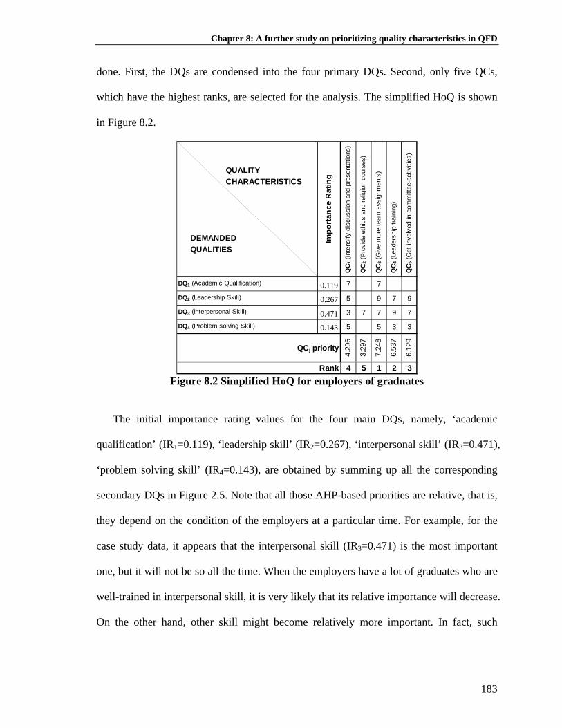
Chapter 8: A further study on prioritizing quality characteristics in QFD
done. First, the DQs are condensed into the four primary DQs. Second, only five QCs,
which have the highest ranks, are selected for the analysis. The simplified HoQ is shown
in Figure 8.2.
QUALITYCHARACTERISTICS
DEMANDEDQUALITIES
0.119 7 7
0.267 5 9 7 9
0.471 3 7 7 9 7
0.143 5 5 3 3Im
porta
nce
Rat
ing
QC 1
(Int
ensi
fy d
iscu
ssio
n an
d pr
esen
tatio
ns)
QC 2
(Pro
vide
eth
ics
and
relig
ion
cour
ses)
QC 3
(Giv
e m
ore
team
ass
ignm
ents
)
QC 4
(Lea
ders
hip
train
ing)
QC 5
(Get
invo
lved
in c
omm
ittee
-act
iviti
es)
2 37.
248
6.53
7
6.12
9
4
QCj priority4.
296
5 13.
297
DQ1 (Academic Qualification)
DQ2 (Leadership Skill)
DQ3 (Interpersonal Skill)
DQ4 (Problem solving Skill)
Rank Figure 8.2 Simplified HoQ for employers of graduates
The initial importance rating values for the four main DQs, namely, ‘academic
qualification’ (IR1=0.119), ‘leadership skill’ (IR2=0.267), ‘interpersonal skill’ (IR3=0.471),
‘problem solving skill’ (IR4=0.143), are obtained by summing up all the corresponding
secondary DQs in Figure 2.5. Note that all those AHP-based priorities are relative, that is,
they depend on the condition of the employers at a particular time. For example, for the
case study data, it appears that the interpersonal skill (IR3=0.471) is the most important
one, but it will not be so all the time. When the employers have a lot of graduates who are
well-trained in interpersonal skill, it is very likely that its relative importance will decrease.
On the other hand, other skill might become relatively more important. In fact, such
183

Chapter 8: A further study on prioritizing quality characteristics in QFD
change in relative importance will always occur. What is important here is to be able to
observe and model the change over time, and make a better decision based upon it.
The department usually carries out a yearly survey to the employers of the graduates.
Due to some reasons, the author has not been able to get all the yearly data. Therefore, an
alternative solution using simulation is suggested to illustrate how the proposed
methodology works in practice. The data from the second period until the ninth period
were simulated from a set of selected randomly generated four-order AHP matrices with
consistency ratio values less than or equal to 10% (see Section 4.2.1.2 for the simulation
method).
Step 4: Fit the DQs’ priorities data change over time using the proposed forecasting
technique. The actual DQs’ priorities data (IR values) for each DQ for nine years are
shown in the first block-column of Table 8.1. For example, the IR values from the
simplified HoQ (Figure 8.2) can be found in the first row (t=1). The data which are shown
next to the first block-column (Table 8.1) are the fitted data using the compositional
double exponential smoothing method (Raharjo et al., 2009). For example, for year 9 (t=9),
the fitted priorities for DQ1, DQ2, DQ3, DQ4 are 0.113, 0.338, 0.403, and 0.146,
respectively.
Table 8.1 Actual, fitted, forecasted, and fitting error values of all IR t IR 1 IR 2 IR 3 IR 4 IR' 1 IR' 2 IR' 3 IR' 4 Ad1 Ad2 Ad3 Ad41 0.119 0.267 0.471 0.143 0.120 0.262 0.468 0.150 - - - -2 0.110 0.252 0.488 0.150 0.120 0.262 0.468 0.150 -0.069 -0.014 0.063 0.0213 0.132 0.265 0.445 0.157 0.114 0.256 0.480 0.150 0.113 -0.005 -0.116 0.0084 0.109 0.283 0.455 0.152 0.124 0.261 0.461 0.155 -0.107 0.101 0.005 0.0015 0.113 0.297 0.465 0.125 0.115 0.275 0.456 0.154 0.011 0.112 0.053 -0.1766 0.129 0.307 0.434 0.129 0.113 0.291 0.460 0.136 0.111 0.035 -0.077 -0.0707 0.119 0.313 0.412 0.156 0.122 0.306 0.443 0.130 -0.054 -0.005 -0.102 0.1608 0.108 0.339 0.403 0.149 0.121 0.317 0.420 0.142 -0.098 0.078 -0.032 0.0539 0.113 0.333 0.385 0.169 0.113 0.338 0.403 0.146 -0.022 -0.037 -0.068 0.127
10 0.117 0.326 0.367 0.1910.087 0.057 0.068 0.106
forecastα*=0.308, StDev of Adi =
184

Chapter 8: A further study on prioritizing quality characteristics in QFD
The third block-column shows the fitting error values which are expressed in terms of
Aitchison distance, see formula (8.3). The optimal parameter (α*=0.308) for the CDES is
derived iteratively by selecting a value between 0 and 1 that gives the minimum average
Aitchison distance. In the last row of Table 8.1, the standard deviation of the forecasting
residual (‘StDev of Adi’), which serves as the measure of future uncertainty, is provided
for each IR.
Before proceeding to the next step, it is interesting to see the validity of the future
uncertainty’s estimate. As explained, the future uncertainty is estimated from the variance
of the forecasting residual which follows Gaussian white noise process with a zero mean
and a constant variance. Table 8.2 shows that the descriptive statistics and the normality
(Anderson-Darling) test of the forecasting residual for each DQ. Table 8.3 further shows
the hypothesis testing of the mean value of the error against zero using Minitab software.
Table 8.2 Descriptive statistics and normality test of forecasting residual
Ad1 -0.014 0.087 -0.107 -0.091 -0.038 0.086 0.113 0.720 -1.000 0.235Ad2 0.033 0.057 -0.037 -0.012 0.015 0.095 0.112 0.340 -1.780 0.274Ad3 -0.034 0.068 -0.116 -0.096 -0.050 0.041 0.063 0.400 -1.480 0.511Ad4 0.015 0.106 -0.176 -0.052 0.014 0.108 0.160 -0.500 0.450 0.715
Mean StDev Min Q1 Median Q3 Max Skewness Kurtosis P-value (A-D Test)
Table 8.3 Mean value test of forecasting residual One-Sample T: Ad ; Ad ; Ad ; Ad4 1 2 3
Test of mu = 0 vs not = 0 Variable N Mean StDev SE Mean 95% CI T P Ad1 8 -0.0144 0.0870 0.0308 (-0.0871; 0.0584) -0.47 0.655 Ad2 8 0.0331 0.0572 0.0202 (-0.0148; 0.0809) 1.63 0.146 Ad3 8 -0.0342 0.0684 0.0242 (-0.0913; 0.0230) -1.41 0.201 Ad4 8 0.0154 0.1061 0.0375 (-0.0733; 0.1042) 0.41 0.693
It can be concluded through the p-values that there is not enough evidence to say that the
forecasting error does not follow normal distribution with a zero mean value. Finally,
185

Chapter 8: A further study on prioritizing quality characteristics in QFD
Table 8.4 shows the independence test using t-test and Ljung-Box test. Both tests confirm
that the Adi are all independently distributed, that is, no autocorrelation exists.
Table 8.4 Independence test of forecasting residual
t-statistic p-value LBQ p-valueLag 1 -0.360 -1.017 0.343 1.478 0.224Lag 2 -0.276 -0.695 0.509 2.491 0.288Lag 1 -0.007 -0.019 0.986 0.000 0.982Lag 2 -0.277 -0.783 0.460 1.021 0.600Lag 1 -0.267 -0.754 0.476 0.812 0.368Lag 2 -0.263 -0.695 0.510 1.731 0.421Lag 1 0.206 0.584 0.578 0.487 0.485Lag 2 -0.154 -0.417 0.689 0.801 0.670
Ad3
Ad4
ACFt-test (2-sided) Ljung-Box test
Ad1
Ad2
Step 5: Obtain the forecasted IR (IRi,k+1) for each DQ using the forecasting method.
The forecasted priorities using the CDES method are shown in the last row (t=10) of
Table 8.1, right below the fitted data. For example, the forecasted priorities for IR1, IR2,
IR3, and IR4, respectively, for the coming period (t=10), are 0.117, 0.326, 0.367, and 0.191.
The graphical plot of the actual, fitted, and forecasted importance rating values (DQs’
priorities) over time is shown in Figure 8.3. The full triangle, diamond, square, and dot are
used to plot the actual data, while the long-dashed, dashed, dash-and-dotted, and dotted
lines are used to show the fitted and forecasted values of IR1, IR2, IR3, and IR4,
respectively.
186
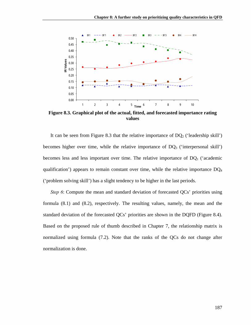
Chapter 8: A further study on prioritizing quality characteristics in QFD
0.00
0.05
0.10
0.15
0.20
0.25
0.30
0.35
0.40
0.45
0.50
1 2 3 4 5 6 7 8 9 10
IR V
alue
s
Time
IR1 IR'1 IR2 IR'2 IR3 IR'3 IR4 IR'4
Figure 8.3. Graphical plot of the actual, fitted, and forecasted importance rating
values
It can be seen from Figure 8.3 that the relative importance of DQ2 (‘leadership skill’)
becomes higher over time, while the relative importance of DQ3 (‘interpersonal skill’)
becomes less and less important over time. The relative importance of DQ1 (‘academic
qualification’) appears to remain constant over time, while the relative importance DQ4
(‘problem solving skill’) has a slight tendency to be higher in the last periods.
Step 6: Compute the mean and standard deviation of forecasted QCs’ priorities using
formula (8.1) and (8.2), respectively. The resulting values, namely, the mean and the
standard deviation of the forecasted QCs’ priorities are shown in the DQFD (Figure 8.4).
Based on the proposed rule of thumb described in Chapter 7, the relationship matrix is
normalized using formula (7.2). Note that the ranks of the QCs do not change after
normalization is done.
187

Chapter 8: A further study on prioritizing quality characteristics in QFD
DQ QC
QC
1 (In
tens
ify d
iscu
ssio
n an
d pr
esen
tatio
ns)
QC
2 (P
rovi
de e
thic
s an
d re
ligio
n co
urse
s)
QC
3 (G
ive
mor
e te
am a
ssig
nmen
ts)
QC
4 (L
eade
rshi
p tra
inin
g)
QC
5 (G
et in
volv
ed in
com
mitt
ee-a
ctiv
ities
)
Impo
rtanc
e R
atin
g (t=
1)
Impo
rtanc
e R
atin
g (t=
2)
…
Impo
rtanc
e R
atin
g (t=
8)
Impo
rtanc
e R
atin
g (t=
9)
Fore
cast
ed IR
(t=1
0)
Fore
cast
ing
Res
idua
l StD
ev (t
=10)
Fore
cast
ing
Res
idua
l Var
ianc
e (t=
10)
DQ1 (Academic qualification) 0.50 0 0.50 0 0 0.119 0.110 … 0.108 0.113 0.117 0.087 0.0076DQ2 (Leadership skill) 0.17 0 0.30 0.23 0.30 0.267 0.252 … 0.339 0.333 0.326 0.057 0.0033DQ3 (Interpersonal skill) 0.09 0.21 0.21 0.27 0.21 0.471 0.488 … 0.403 0.385 0.367 0.068 0.0047DQ4 (Problem solving skill) 0.31 0 0.31 0.19 0.19 0.143 0.150 … 0.149 0.169 0.191 0.106 0.0113Mean of forecasted QCj priority 0.206 0.078 0.294 0.212 0.211
StDev of forecasted QCj priority 0.091 0.031 0.096 0.064 0.064 Figure 8.4 The DQFD for the employers of graduates
What is worth highlighting here is the use of the forecasted QCs’ priorities, which are
derived from the future needs of the customer, as a basis for optimizing the QCs. By doing
so, the department may better tackle the time-lag problem discussed in Section 1.1 in the
sense that it may better anticipate the future needs of the employer early in the education
process. Suppose that we are now at the ninth period (t=9), that is, year nine. It is known
that the department produces most of the graduates every year (in the annual
commencement ceremony). Therefore, for this year planning (year nine), the basis of the
decision, for example, budget allocation, should be on the next year’s needs, namely, the
forecasted priorities at year ten. Such action will help the department make a better
decision in the sense that it will train at least the last year students the required skills so
that when those students graduate next year (year ten), they will hopefully meet the skills
required in the job place better.
In short, the above example shows the importance of taking into account the change of
customer-needs’ priorities during service creation time, that is, during one year education
188

Chapter 8: A further study on prioritizing quality characteristics in QFD
period before the students graduate. Note that the example assumes that the real rate of
change is yearly. The next two subsections will provide a further analysis on the results
obtained from the first six steps for decision making purpose, that is, for optimizing and
prioritizing the QCs using the two proposed approaches.
8.4.1 Using optimization model 1: Utilitarian approach
Step 7a: Plot the cumulative density function (CDF) of all QCs according their mean
and standard deviation values together in one graph. The CDF of all QCs are shown in
Figure 8.5.
0.70.60.50.40.30.20.10.0-0.1-0.2
100
80
60
40
20
0
x
F(X
<=
x)
QC1QC2QC3QC4QC5
CDF of QC1, QC2, QC3, QC4, QC5
Figure 8.5 Plot of CDF of all QCs
Step 8a: Check for first-order dominance using the CDF curves. For normal
distribution, it is well-known that if A~ ),( AAN σμ and B~ ),( BBN σμ , then A will first
order stochastically dominates B, or A B, if and only if )1(f BA μμ > and BA σσ = .
Furthermore, A will second order stochastically dominate B, or A B, if and only if )2(f
BA μμ ≥ and BA σσ ≤ with at least one strong inequality holds (see Levy, 1998). By
189
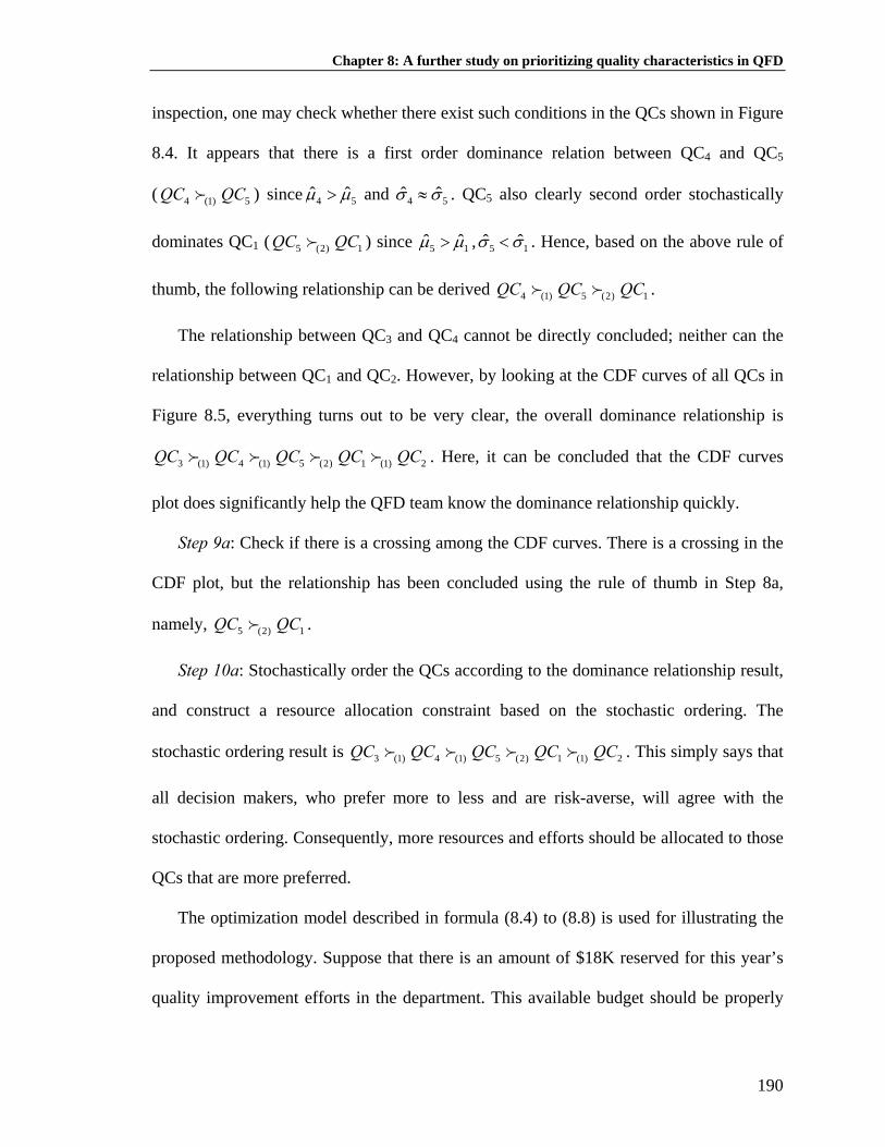
Chapter 8: A further study on prioritizing quality characteristics in QFD
inspection, one may check whether there exist such conditions in the QCs shown in Figure
8.4. It appears that there is a first order dominance relation between QC4 and QC5
( ) since4 (1) 5QC QCf 4ˆ ˆ5μ μ> and 4ˆ ˆ5σ σ≈ . QC5 also clearly second order stochastically
dominates QC1 ( ) since 5 (2) QCf 1QC 5 1ˆ ˆμ μ> , 5ˆ ˆ1σ σ< . Hence, based on the above rule of
thumb, the following relationship can be derived . 4 (1) 5 (2) 1QC QCf f
1 (1) 2QC QCf f
QC
5 (2)QC
The relationship between QC3 and QC4 cannot be directly concluded; neither can the
relationship between QC1 and QC2. However, by looking at the CDF curves of all QCs in
Figure 8.5, everything turns out to be very clear, the overall dominance relationship is
. Here, it can be concluded that the CDF curves
plot does significantly help the QFD team know the dominance relationship quickly.
3 (1) 4QC QCf f
5 (f
( (1)f f1) QC
2) QC
5 (2) 1QC
1
2QC
(1) 4QCf f
Step 9a: Check if there is a crossing among the CDF curves. There is a crossing in the
CDF plot, but the relationship has been concluded using the rule of thumb in Step 8a,
namely, QC .
Step 10a: Stochastically order the QCs according to the dominance relationship result,
and construct a resource allocation constraint based on the stochastic ordering. The
stochastic ordering result is QC . This simply says that
all decision makers, who prefer more to less and are risk-averse, will agree with the
stochastic ordering. Consequently, more resources and efforts should be allocated to those
QCs that are more preferred.
3 (1)
The optimization model described in formula (8.4) to (8.8) is used for illustrating the
proposed methodology. Suppose that there is an amount of $18K reserved for this year’s
quality improvement efforts in the department. This available budget should be properly
190

Chapter 8: A further study on prioritizing quality characteristics in QFD
allocated for the fulfillment of the QCs so that the future total customer satisfaction level
will be maximized. According to the department’s decision, the cost of improvement of
each QC to achieve its maximum possible target value (best possible state), namely, the
fulfillment cost (Cj) is $7K, $6K, $6K, $11K, $9K, for QC1, QC2, QC3, QC4, QC5,
respectively. For example, if an amount of $11K is allocated to QC4, in this case for
developing ‘leadership training’, then this QC may be improved to its best possible state.
One example of ways for developing ‘leadership training’ might be asking reputable
leaders to train the students or to provide some workshops.
Then, for the sake of simplicity, the minimum satisfaction level for each DQ (Xie et al.,
2003) is assumed to be the same, that is, 50%, or 4,...,1,5.0 =∀= iSLi . It is again
assumed that there is no difference in the amount of QC fulfillment, thus
4,...,1,0 =∀= rrδ . Note that the last value of the subscript r, that is, four (r=4), denotes
the number of the stochastic dominance constraints used to represent the stochastic
ordering result (see formula (8.7) and (8.15)). The complete formulation according to the
total customer satisfaction optimization model in (8.4)-(8.8) is as follows.
Maximize Z = 1 2 3 40 029 0 013 0 049 0 019 0 024 5X X X X X+ + + +. . . . . (8.12)
Subject to:
1 2 3 4 5 18X X X X X+ + + + ≤ (8.13)
1 30 071 0 083 50X X+ ≥. . % ; 1 3 4 50 024 0 05 0 021 0 033 50X X X X+ + + ≥. . . . % ;
1 2 3 4 50 013 0 035 0 035 0 025 0 024 50X X X X X+ + + + ≥. . . . . % ;
1 3 4 50 045 0 052 0 017 0 021 50X X X X+ + + ≥. . . . % (8.14)
3 46 11 0X X− ≥ ; 4 511 9 0X X− ≥ ;
191

Chapter 8: A further study on prioritizing quality characteristics in QFD
5 19 7 0X X− ≥ ; 1 27 6X X− ≥ 0 (8.15)
10 7 1X≤ ≤ ; 20 6 1X≤ ≤ ; 30 6X 1≤ ≤ ;
40 11 1X≤ ≤ ; 50 9X≤ 1≤ (8.16)
The solution for the above optimization model is shown in Table 8.5. An example of
interpreting the result is as follows. An amount of $6K should be allocated to QC3, which
results in 100% fulfillment of its target value, while none of the budget should be
allocated to QC2. This solution is fully consistent with the stochastic
( ) since QC3 is the most preferred one, while QC2
is the least preferred. The total customer satisfaction that can be obtained from this
solution is 55% (Z=55%).
3 (1) 4 (1) 5 (2) 1 (1) 2QC QC QC QC QCf f f f
Table 8.5 Optimization results with SD constraint
Variable X 1 X 2 X 3 X 4 X 5
Allocation 0.27 0.00 6.00 6.45 5.28
Fulfillment 3.8% 0% 100% 58.7% 58.7%
With SD Constraint (Z=55%)
Now, suppose if the stochastic dominance constraints, those expressions in (8.15), are
relaxed and the model is solved once again using the software. The purpose here is to
illustrate what would happen if one ignored the future uncertainty factor in the customer
needs. The result is shown in Table 8.6. In contrast to the previous result, the result,
although having a slightly higher customer satisfaction value (Z=57%), is totally not in
agreement with the stochastic ordering. For example, QC2, which is the least preferred
192

Chapter 8: A further study on prioritizing quality characteristics in QFD
one, has 27% level of fulfillment while none of the resource is allocated to QC4, which is
much more preferred than QC2.
Table 8.6 Optimization results without SD constraint
Variable X 1 X 2 X 3 X 4 X 5
Allocation 1.35 1.65 6.00 0.00 9.00
Fulfillment 19.4% 27.4% 100% 0% 100%
Without SD Constraint (Z=57%)
In sum, the optimization model results in an optimal policy to allocate the department
yearly budget. The policy may be considered as ‘optimal’ not only because it has taken
into account the resources limitation, but it has also considered the future needs of the
customer along with their uncertainty. Furthermore, the budget allocation policy has also
taken into account the change of the external customer’s needs during the service creation
process, that is, during the one year education time before the students graduate.
Another finding is that unless the future uncertainty factor, which is represented by the
variance of the forecasting residual, in the DQs is taken into account, it is very likely that
one might end up with a fallacious allocation policy with respect to the decision maker’s
attitude towards risk in the future needs. This is also to say that considering the point
estimate alone is not sufficient and might lead to misleading optimization results. After
optimizing the fulfillment of each QC, the QFD team may use the result for other
subsequent downstream analysis.
8.4.2 Using optimization model 2: Non-utilitarian approach
Step 7b: Apply the mathematical model below (Raharjo et al., 2006) to prioritize
and/or optimize the QCs. Using all the information provided in Section 8.4.1, another
193

Chapter 8: A further study on prioritizing quality characteristics in QFD
approach can be used. The only difference here is the definition of the decision variable
(Xj). The decision variable indicates the inclusion or exclusion of a QC rather than its
fulfillment, thus, once it is included it implies that it is fully fulfilled since an amount of Cj
is allocated.
Step 8b: Define the model parameters based on decision maker’s preference. Assume
that the target values for the mean and the standard deviation are, respectively, 100% (and
0% ( *Y = 100%; = 0%). It is also known that the education institution places a higher
emphasis on the mean value rather than variability value. Thus, the value of
*S
α is assigned
to be 0.1, while the value of β =0.6. The normalized mean and standard deviation values
for the forecasted QCs’ priorities in Figure 8.4 are ∈normjy {20.6, 7.8, 29.4, 21.2, 21.2}
and {26.2, 9.1, 27.7, 18.6, 18.4}. Then, the mathematical model can be written as
follows:
∈normjs
5
22
2
22
1
22
6.04.18
1.01002.21
6.01.9
1.01008.7
6.02.26
1.01006.20
X
XXZMin
⎥⎥⎦
⎤
⎢⎢⎣
⎡⎟⎠⎞
⎜⎝⎛+⎟
⎠⎞
⎜⎝⎛ −
+
+⎥⎥⎦
⎤
⎢⎢⎣
⎡⎟⎠⎞
⎜⎝⎛+⎟
⎠⎞
⎜⎝⎛ −
+⎥⎥⎦
⎤
⎢⎢⎣
⎡⎟⎠⎞
⎜⎝⎛+⎟
⎠⎞
⎜⎝⎛ −
= K (8.20)
Subject to:
%505.05.0 31 ≥+ XX ; %503.023.03.017.0 5431 ≥+++ XXXX ;
%5021.027.021.021.009.0 54321 ≥++++ XXXXX
%5019.019.031.031.0 5431 ≥+++ XXXX
;
(8.21)
18911667 54321 ≤++++ XXXXX (8.22)
{ } 5 ,...,2 ,1 1 ,0 =∀∈ jX j (8.23)
194
Chapter 8: A further study on prioritizing quality characteristics in QFD
Step 9b: Solve the model and conduct sensitivity analysis of the parameters’ change.
The above model can be solved easily using Excel-solver or other software. Considering
the current constraints, namely, the maximum budget is $18K and the minimum
satisfaction level for each DQ is 50%, no solution can be obtained. In other words, it is
impossible to achieve 50% satisfaction level for each customer need if there is only $18K
available. If the minimum satisfaction level is slightly lowered to 48%, then the optimal
solution is to select QC3 and QC4. This solution is in line with the result from the other
approach (subsection 8.4.1).
Among the selected QCs, further prioritization can still be done based on the value of
the quality loss incurred for the corresponding QC. Thus, in this case, the further
prioritization, in the order of the lowest quality loss, is QC3 and then QC4. This is again
consistent with the SD results in previous subsection. A sensitivity analysis can further be
carried out for the effect of changing the parameters, see Raharjo et al. (2006) for an
example.
Step 10b: Proceed with downstream QFD analysis using the selected QCs. The focus
of the next downstream QFD process should be on the QC3 first, and followed by QC4.
There are at least two main advantages of using this non-utilitarian approach. First, it
may not only efficiently prioritize the QCs, but also can effectively reduce the size of the
HoQ. This is a worth noting advantage since most of the QFD applications are inherently
plagued with the problem of a prohibitively large-sized HoQ which makes the QFD
process very tedious and time consuming. Second, as has been shown, a further
prioritization process in the optimal solution, that is, among the selected QCs, can still be
carried out based on the quality loss value incurred.
195

Chapter 8: A further study on prioritizing quality characteristics in QFD
8.5 Discussions
8.5.1 Selection of forecasting technique
There are at least two reasons why the CDES method (Raharjo, et al., 2009) is
selected. First, it is suitable for the situation when there is only a minimal number of
historical data. Second, it is relatively simple and time-efficient compared to other time
series methods, especially for modeling the dynamics of AHP-based priorities. It is
possible that the CDES method may end up with errors which do not follow Gaussian
white noise process. In such case, other forecasting techniques, such as multivariate time
series technique, is called for. What is more important here is the fact that a proper and
adequate forecasting technique will result in Gaussian white noise error, of which variance
is proposed as the measure of future uncertainty of the forecasted points.
8.5.2 A possible implication to development of innovative products
The proposed methodology might be potentially useful for the possible application of
QFD in developing innovative products, such as consumer electronics products which are
launched in a highly dynamic market (Minderhoud and Fraser, 2005). In a highly dynamic
market, the change of customer preference may have a great impact on the company
(Bhattacharya, 1998). The cost of not producing a product that the customer wants might
be tremendously large, it is therefore very reasonable to make extra efforts to monitor and
follow the customer preference change over time.
Consider the cellular phone, in the past, the importance of ‘user-interaction’ (tactual
quality) might be relatively lower than the importance of ‘good audio function’ (audio
quality), but nowadays, the importance of ‘user-interaction’, such as the touch-screen
196

Chapter 8: A further study on prioritizing quality characteristics in QFD
command, may be relatively higher than the importance of ‘good audio function’, such as
FM Radio. So the relative change over time of one attribute over the other attributes is
precisely the situation where the DQFD explained in this thesis might have a possible
contribution towards the development of innovative products.
Prescriptively speaking, to accurately assess the importance of those DQs over time, a
series of well-controlled customer surveys to a specific market segment should be done.
However, this will not only involve a huge cost, but also a considerable amount of time.
Another alternative way, which is more descriptive, is to infer the priorities by observing
the change of commercial specification of a product over time. The reason is because the
firm will not put anything unimportant in their top advertisement list. Interestingly, a
recent study by Hsee et al. (2009) found that the product specification also influences
customer preference. There appears to be a reciprocal effect between customer preference
and commercial specification. However, this issue is beyond the scope of this thesis.
The example of the change of commercial specification of a cellular phone for a
specific segment over time is shown in Table 8.7. The data were taken from Nokia official
website3 . It is the published commercial specification for Nokia 6000s series phones,
which are specifically targeted for mainstream market, from 2007 to 2008. All the 6000s
series phones’ commercial specifications during the last two years were first observed (see
Appendix C and D). Then, for each quarter which is intended for the ‘planned market
introduction’ (P.M.I, in Table 8.7) of the specific series, one representative series is
selected. Note that the 6000s series are not always launched every quarter.
3 Source: http://www.nokia.com/press/media_resources/documents/
197

Chapter 8: A further study on prioritizing quality characteristics in QFD
Table 8.7 Example of customer preference dynamics from commercial specification P.M.I Q1, 2007 Q2, 2007 Q3, 2007 Q4, 2007 Q2, 2008 Q3, 2008
Model Nokia 6086 Nokia 6110 Nokia 6267 Nokia 6301 Nokia 6300i Nokia 6600f
Key Feature
• Stylish fold design with intuitive keypad and large colordisplay • Music player (MP3, MP4, AAC, AAC+, eAAC+, WMA) • Enhanced audio quality • …
• Navigator key for fast and easy access
• 3G multimedia: video call, fast download of games, music, video and ringing tones.
• …
• Sleek and compact fold design with large keypad and clear high-resolution color display • Dedicated keys for easy access to music • High quality video recording up to DVD resolution and playback in full VCR quality • …
• Clear and easy to read display with 16.7 million colors • …
• Nokia Maps to help navigate and find the way
• …
• 240x320 OLED 16 million color main display
• Hidden outer display • Tap commands: double tap to turn on hidden outer display / snooze alarm / first silence, then reject call
• …
Additional Features
• Stereo FM Radio with Visual Radio • …
• Music player supporting MP3, MP4, M4A, AAC, eAAC+, WMA
• Stereo FM radio and support for Visual Radio
• …
• Music player supporting MP3, MP4, AAC, eAAC+ and Windows Media Audio • FM stereo radio supporting Visual Radio • …
• Music player supporting MP3, AAC, eAAC+ • FM stereo radio supporting Visual Radio • Nokia Audio Messaging • …
• 2.0” TFT QVGA color display
• Music player (MP3, AAC, AAC+, eAAC+, WMA) and FM stereo radio with RDS
• …
• Stereo music player supporting MP3, AAC, AAC+, eAAC+ and WMA, and stereo FM Radio
• …
For the sake of simplicity, only three DQs, which represent customer’s needs, are
observed, namely, ‘Good audio quality (A)’, ‘Good display (D)’, and ‘Good interaction or
tactual quality (T)’. It can be seen from Table 8.7, that ‘A’ is very much important in first
quarter of 2007. The ‘music player’ (italicized) is considered as the key feature. After a
while, it becomes an additional feature. For ‘Good display (D)’ (underlined), it is quite
relative, in some quarters, this feature is very important, while not in some other quarters.
Finally, the tactual feature ‘T’ (highlighted) seems to become increasingly important.
Initially, there is ‘intuitive key pad’, then ‘dedicated keys’, and ‘tap commands’ in the end.
In other words, this feature has become more and more important relatively compared to
the others.
In brief, the above example has shown that the importance of customer’s needs change
over time. The main reason is that it is relative and may depend on a number of factors at
a certain point of time. The worth noting point here is that this observation might shed
some light to the possibility of applying the method and/or approaches proposed in this
198

Chapter 8: A further study on prioritizing quality characteristics in QFD
thesis in developing more innovative products. A further discussion is provided in Section
9.3 (Chapter 9).
8.6 Conclusions
The purpose of this chapter was to provide a possible answer to the research question
“How to make decision in a QFD analysis with respect to the dynamics in the house of
quality?” This chapter has answered the question by proposing a systematic methodology,
which may use two kinds of decision making approaches, to prioritize or optimize the
QCs with respect to the future needs of the customer. The methodology employs the
modeling technique proposed in Chapter 4 as the tool to forecast the dynamics of DQs’
priorities.
To show how the methodology works in practice, the case study described in Chapter
2 is used to provide the contextual setting. The notion of future uncertainty to improve
forecast precision has also been introduced. It is hoped that the proposed methodology
might help QFD-users better deal with the future needs of the customer, especially in
tackling the problem described in Section 1.1.
The proposed methodology places a heavy emphasis on the need to monitor and
follow the change of customer’s preference over time. It is because a timely update of
customer needs information may provide useful feedback for the company to react
differently and continuously over time as to formulate strategies or to upgrade its products
or services to meet the changing needs of its customer.
From a methodological standpoint, there are three areas that might be worth
investigating for future work. First, it might be interesting to investigate how one may deal
199

Chapter 8: A further study on prioritizing quality characteristics in QFD
200
with the condition when there will be inclusion of a new customer need (DQ) or exclusion
of an old one as the passage of time. Second, in the use of stochastic dominance approach
in QFD, how one may know precisely the percentage of the resources to be allocated in
the stochastically-ordered QCs remains a challenging issue to be addressed. Furthermore,
if the QFD team has a risk seeking attitude, the proposed stochastic dominance approach
may no longer apply. Third, the incorporation of fuzzy logic theory in the optimization
models may also be considered.
From a practical standpoint, a worth noting aspect is the difference between the real
rate of change of customer preference and the observation period, that is, how often the
data should be collected. For example, it would be of little value if the customer needs’
information is collected monthly, while the real change rate is yearly. Finally, more real-
world applications of the proposed methodology would certainly be of great value to
showcase the usefulness of the dynamic QFD in practice.

Chapter 9: Conclusion and future research
CHAPTER 9
CONCLUSION AND FUTURE RESEARCH
“To keep an important thing important is an important thing” (Raharjo, 2009: reflection on thesis)
9.1 Conclusion
The main objective of this thesis was to develop novel methods and/or approaches for
enhancing the use of QFD, especially in combination with the AHP, in dealing with the
dynamics during product or service creation process. With respect to the three specific
objectives set in Chapter 1, the conclusion can be stated as follows.
1. The thesis has demonstrated the usefulness of the AHP in QFD and has provided a
better use of it by proposing a generalized use of the AHP in QFD.
2. The thesis has developed a new method to model the dynamic of AHP-based
priorities in the house of quality.
3. The thesis has developed two methods and/or approaches for decision making with
respect to the modeling results as to continually meet or exceed the needs of the
customer.
The key message in this thesis is that QFD practitioners, to be able to better deal with
the change during product or service creation process (Section 1.1), need to continually
monitor and follow the change of over time. By doing so, not only a timely update of
customer’s needs information may be obtained, but also the future needs may be projected
based on the pattern of past data. As shown in the education case study example, the
future needs should become the basis of the decision making so that the “product”, taking
into account its creation time, may eventually meet the changing needs of the customer. In
201

Chapter 9: Conclusion and future research
addition, for the subsequent periods, it is also important to keep updating the customer’s
needs data so that the QFD practitioners may react differently and continuously over time
with better strategies as to upgrade its products or services.
To briefly conclude the thesis, an illustration using the concept of “doing the right
things right the first time continuously” is employed. Almost all previous QFD research
focuses on “doing the right things the first time”, that is, to begin with the needs of the
customer in early stage of product or service development process. What makes the thesis
different is that it attempts to complement the existing QFD research by not only doing the
right things the first time, but also doing it right continuously. Hence, it is hoped that this
may eventually increase the possibility of a successful QFD application.
9.2 Major contributions
All the research efforts in order to achieve the objective are reflected in the nine papers
in Appendix E; almost all of them have been published in internationally reputable
journals1. The major contributions towards the advancement of QFD methodology and
analysis can be summarized into three points, which correspond to Chapter 2 to Chapter 8,
as follows. Note that these contributions are mainly on the theoretical development of
QFD considering that the methods and/or approaches have not yet been proven to have a
demonstrated value in tackling the change during product creation process in industries.
1. The use of the AHP in QFD has been thoroughly studied. From a practical standpoint,
the QFD-AHP method has been successfully applied in improving higher education
quality of an industrial engineering department (Chapter 2). From a theoretical point
1 Science Citation Index journals
202

Chapter 9: Conclusion and future research
of view, the use of the AHP in QFD has been significantly enhanced using the
generalized model (Chapter 3). The generalized model has been tested on a realistic
example based on interview and questionnaire data. Additionally, a new finding on
the weakness of AHP when the number of alternatives gets larger is also provided
(Chapter 2). Such finding might serve as useful information when dealing with a
large-sized house of quality.
2. It has been shown that the AHP may be considered as a beneficial tool for deriving
DQs’ priorities in QFD. Besides, it can also be applied to obtain the DQs’ competitive
assessment due to its relative measurement approach (Chapter 6). In response to the
increasingly extensive research on AHP’s use in QFD (Carnevalli and Miguel, 2008;
Ho, 2008) in recent years, a new method to model the priorities’ dynamics is
proposed (Chapter 4). The method is very useful in modeling the AHP-based
priorities’ dynamics, especially for better tackling the change of customer’s needs and
competitors’ performance during product or service creation process. Furthermore,
the method has also been applied to model Kano’s model dynamics (Chapter 5). It is
the first time that the life cycle of quality attributes is analyzed quantitatively via
mathematical modeling.
3. To improve the forecast precision, an interval estimate, in addition to the point
estimate of future needs, is suggested (Chapter 8). The interval estimate, which at the
same time serves as the estimate of future uncertainty, is derived from the variance of
forecasting residual. A closer look at the relationship matrix with respect to the need
of normalization is also carried out (Chapter 7). This issue is of great importance
since the relationship matrix values, together with the DQs’ priorities, determine the
final output of the HoQ, namely, the QCs’ priorities. Finally, two kind of optimization
203

Chapter 9: Conclusion and future research
models are proposed to facilitate the decision making process with respect to the
future needs (Chapter 8).
9.3 A note on the practical implication of DQFD for innovative products
A study by Griffin (1992) on evaluating QFD’s use in US firms has identified three
factors that increase the success of a QFD application, namely, service projects, less
complex projects, and incremental change. In line with her finding, this thesis has
attempted to apply the dynamic QFD (DQFD) to a relatively small service project, namely,
the education case study (Chapter 2). As has been partly addressed in Section 8.5.2, this
section further discusses the potential of the proposed methods and/or approaches in this
thesis in developing innovative products in a broader perspective. Some important
questions to address may include what kind of innovative product that can be developed
using DQFD, what type of innovation is most suitable, which market segment, and so
forth.
A recent study by Miguel (2007) found that QFD may help develop innovative
products, but it is limited to additions to existing lines, product repositioning, and product
improvement. In line with his finding, the extent to which the methods and/or approaches
proposed in this thesis might be useful is limited to incremental products, as opposed to
breakthrough or radical product. The term ‘incremental products’ here is used to refer to a
set of products which are continuation of the existing ones, for example, by improving or
adding existing features. One example of the products may be the consumer electronics
products of which features are enhanced over time, such as televisions or cellular phones.
204

Chapter 9: Conclusion and future research
Furthermore, the uncertainty that is dealt with in this thesis is parametric uncertainty,
as opposed to structural uncertainty, in the sense that the structure of the problem is
already known and only the parameters are uncertain. For example, the customer’s needs
are already known, but the parameter (importance rating value) is uncertain. Finally, to
such kind of products, the most appropriate target market might be the early and/or late
majority market (Rogers, 2003).
Consider again the cellular phone example described in Section 8.5.2, by observing
the change of the features in the commercial specification, one may infer that the relative
importance of the existing customer’s needs (DQs) changes over time. Suppose the
product creation time of the cellular phone is one quarter, and so is the real rate of DQs’
importance change. A quarterly observation is therefore carried out to monitor and follow
the change of customer’s needs over time. Then, for the purpose of developing the 6000s
series cellular phones which will be launched next quarter, there is no reason to not
consider the forecasted importance or priorities for next quarter as the main basis of
customer’s needs information. This is where the proposed methods and/or approaches in
this thesis might be useful. Certainly, this case is simplified for the sake of illustration
purpose.
In short, it can be said that the proposed methods and/or approaches should neither be
intended for developing really new products (clean sheet designs) nor more complex
projects (Griffin, 1992). Such information may help set the boundary of what to expect
from the proposed methods and/or approaches in this thesis, especially when using QFD
in developing more innovative products.
205

Chapter 9: Conclusion and future research
206
9.4 Future research
There are two quite important assumptions in this thesis, of which relaxation may open
up several interesting issues for future research. First, it is assumed that the real rate of
change is known and the same as the length of product or service creation time (see
Chapter 8). Second, it is assumed that the customer’s needs (DQs) have already existed
from the beginning of the analysis and the only change is in their relative importance or
priorities (see Chapter 1).
With respect to the first assumption, this thesis has not delved into the case when there
is a difference between the rate of change and the length of product or service creation
time. For example, if the length of product creation time is one year and the rate of change
is monthly, then it would be interesting to study when the product concept may still be
kept open to change. This is also related to the use of further matrices in the QFD, apart
from the house of quality. In addition, the rate of change and the length of product or
service creation time might be uncertain. How to take into account such issue in DQFD
analysis may deserve an attention for future work.
With respect to the second assumption, a study on how QFD practitioners may deal
with the situation when there will be inclusion of a new customer need or exclusion of an
old one along the time might be worth pursuing. Other more specific future research
directions can be found in the final section of Chapter 2 to Chapter 8.

References
REFERENCES
Aczel, J., Saaty, T.L. (1983), Procedures for Synthesizing Ratio Judgments, Journal of Mathematical Psychology, 27, 93-102.
Aitchison, J. (1982), The Statistical Analysis of Compositional Data, Journal of the Royal Statistical Society, Series B (Methodological), 44(2), 139-177.
Aitchison, J. (2003), The Statistical Analysis of Compositional Data, Reprint, Blackburn Press, Caldwell, NJ.
Aitchison, J., Barceló-Vidal, C., Martín-Fernández, J.A., Pawlowsky-Glahn, V. (2000), Logratio Analysis and Compositional Distance, Mathematical Geology, 32(3), 271-275.
Akao, Y., Mazur, G.H. (2003), The Leading Edge in QFD: Past, Present and Future, International Journal of Quality & Reliability Management, 20(1), 20-35.
Ames, A.E., Mattucci, N., Macdonald, S., Szonyi, G., Hawkins, D.M. (1997), Quality Loss Functions for Optimization across Multiple Response Surfaces, Journal of Quality Technology, 29(3), 339-346.
Armacost, R.L., Componation, P.J., Mullens, M.A., and Swart, W.W. (1994), An AHP Framework for Prioritizing Customer Requirements in QFD: an industrialized housing application, IIE Transactions, 26(4), 72-79.
Aytaç, A., Deniz, V. (2005), Quality Function Deployment in Education: A Curriculum Review, Quality & Quantity, 39, 507-514.
Bard, J.F., Sousk, S.F. (1990), A Tradeoff Analysis for Rough Terrain Cargo Handlers using the AHP: An Example of Group Decision Making, IEEE Transactions on Engineering Management, 37(3), 222–228.
Belton, V., Gear, T. (1983), On a Short-coming of Saaty’s Method of Analytic Hierarchies, Omega, 11(3), 228-230.
Bergman, B., Klefsjö, B. (2003), Quality from Customer Needs to Customer Satisfaction, Studentlitteratur, Lund, Sweden.
Bhattacharya, S., Krishnan, V., Mahajan, V. (1998), Managing New Product Definition in Highly Dynamic Environments, Management Science, 44(11), S50-S64.
Bier, I.D., Cornesky, R. (2001), Using QFD To Construct A Higher Education Curriculum, Quality Progress, April, 64-68.
Braadbaart, O. (2007), Collaborative Benchmarking, Transparency and Performance: Evidence from The Netherlands Water Supply Industry, Benchmarking: An International Journal, 14(6), 677-692.
Brackin, P. (2002), Assessing Engineering Education: An Industrial Analogy, International Journal of Engineering Education, 18(2), 151-156.
Brombacher, A.C., Sander, P.C., Sonnemans, P.J.M., Rouvroye, J.L. (2005), Managing Product Reliability in Business Processes ‘under pressure’, Reliability Engineering and System Safety, 88, 137-146.
Brown, R.G., Meyer, R.F. (1961), The Fundamental Theorem of Exponential Smoothing, Operation Research, 9, 673-685.
Brunsdon, T.M., Smith, T.M.F. (1998), The Time Series Analysis of Compositional Data, Journal of Official Statistics, 14(3), 237-253.
Burke, E., Kloeber, J.M.Jr., Deckro, R.F. (2002), Using and Abusing QFD Scores, Quality Engineering, 15(1), 9-21.
Büyüközkan, G., Ertay, T., Kahraman, C., Ruan, D. (2004), Determining the Importance Weights for the Design Requirements in the House of Quality Using the Fuzzy Analytic Network Approach, International Journal of Intelligent Systems, 19, 443-461.
Büyüközkan, G., Feyzioğlu, O. (2005), Group Decision Making to Better Respond Customer Needs in Software Development, Computers & Industrial Engineering, 48, 427–441.
207

References
Calantone, R.J., Di Benedetto, C.A., Schmidt, J.B. (1999), Using the Analytic Hierarchy Process in New Product Screening, Journal of Product Innovation Management, 16, 65-76.
Camp, R.C. (1995), Business Process Benchmarking: Finding and Implementing Best Practices, ASQC Quality Press, Milwaukee, WI.
Carnevalli, J.A. and Miguel, P.A.C. (2008), Review, Analysis and Classification of the Literature on QFD—Types of Research, Difficulties and Benefits, International Journal of Production Economics, 114, 737-754.
Chan, F.T.S., Henry, H.K., Lau, C.W. and Ralph, W.L.Ip (2006), An AHP Approach in Benchmarking Logistics Performance of the Postal Industry, Benchmarking: An International Journal, 13(6), 636-61.
Chan, L.K., Wu, M.L. (2002a), Quality Function Deployment: A Literature review, European Journal of Operational Research, 143, 463-497.
Chan, L.K., Wu, M.L. (2002b), Quality Function Deployment: A Comprehensive Review on Its Concepts and Methods, Quality Engineering, 15(1), 23-35.
Chen, J., Chen, J.C. (2001), QFD-based Technical Textbook Evaluation- Procedure and a Case Study, Journal of Industrial Technology, 18(1), 1-8.
Chen, S.H., Yang, C.C. (2004), Applications of Web-QFD and E-Delphi Method in the Higher Education System, Human Systems Management, 23, 245-256.
Chen, Y., Fung, R.Y.K., Tang, J. (2006), Rating Technical Attributes in Fuzzy QFD by Integrating Fuzzy Weighted Average Method and Fuzzy Expected Value Operator, European Journal of Operational Research, 174, 1553-1566.
Chen, Y., Tang, J., Fung, R.Y.K., Ren, Z. (2004), Fuzzy Regression-based Mathematical Programming Model for Quality Function Deployment, International Journal of Production Research, 42(5), 1009-1027.
Chen, Y.M., Huang, P.N. (2007), Bi-negotiation Integrated AHP in Suppliers Selection, Benchmarking: An International Journal, 14(5), 575-93.
Chopra, S., Sodhi, M.S. (2004), Managing Risk to Avoid Supply-Chain Breakdown, MIT Sloan Management Review, 46(1), 53-61.
Chou, S.M. (2004), Evaluating the Service Quality of Undergraduate Nursing Education in Taiwan – using Quality Function Deployment, Nurse Education Today, 24, 310-318.
Chuang, P.T. (2001), Combining the Analytic Hierarchy Process and Quality Function Deployment for a Location Decision from a Requirement Perspective, International Journal of Advanced Manufacturing Technology, 18, 842–849.
Cohen, L. (1995), Quality Function Deployment: How to Make QFD Work for you, Addison-Wesley Publishing Company, MA.
Cooper, R.G., Kleinschmidt, E.J. (1987), New Products: What Separates Winners from Losers?, Journal of Product Innovation Management, 4, 169-184.
Cooper, R.G., Kleinschmidt, E.J. (1995), Benchmarking the Firm’s Critical Success Factors in New Product Development, Journal of Product Innovation Management, 12, 374-391.
CQM (1993), A Special Issue on Kano’s Methods for Understanding Customer-defined Quality, The Center for Quality Management Journal, 2(4), 3-35.
Cristiano, J.J., Liker, J.K., and White III, C.C. (2001), Key Factors in the Successful Application of Quality Function Deployment (QFD), IEEE Transactions on Engineering Management, 48(1), 81- 95.
Cristiano, J.J., Liker, J.K., White III, C.C. (2000), Customer-Driven Product Development Through Quality Function Deployment in the U.S. and Japan, Journal of Product Innovation Management, 17, 286-308.
Demirtas, E.A., Ustun, O. (2007), Analytic Network Process and Multi-period Goal Programming Integration in Purchasing Decisions, Computers & Industrial Engineering, in press.
Den Ouden, E. (2006), Development of a Design Analysis Model for Consumer Complaints: Revealing a New Class of Quality Failure, PhD Thesis, Eindhoven, The Netherlands: Eindhoven University of Technology.
208

References
Den Ouden, E., Lu, Y., Sonnemans, P.J.M., Brombacher, A.C. (2006), Quality and Reliability Problems from a Consumer’s Perspective: an Increasing Problem Overlooked by Businesses?, Quality and Reliability Engineering International, 22, 821-838.
Dey, P.K. (2004), Decision Support System for Inspection and Maintenance: A Case Study of Oil Pipelines, IEEE Transactions on Engineering Management, 51(1), 47-56.
Dey, P.K., Hariharan, S. and Despic, O. (2008), Managing Healthcare Performance in Analytical Framework, Benchmarking: An International Journal, 15(4), pp. 444-468.
Duffuaa, S.O., Al-Turki, U.M., Hawsawi, F.M. (2003), Quality Function Deployment for Designing a Basic Statistics Course, International Journal of Quality & Reliability Management, 20(6), 740-750.
Dyer, R.F., Forman, E.H. (1992), Group Decision Support with the Analytic Hierarchy Process, Decision Support Systems, 8, 99-124.
Ermer, D.S. (1995), Using QFD Becomes an Educational Experience for Students and Faculty, Quality Progress, 28(5), 131-136.
Ertay, T., Büyüközkan, G., Kahraman, C., Ruan, D. (2005), Quality Function Deployment Implementation Based on Analytic Network Process with Linguistic Data: An Application in Automotive Industry, Journal Intelligent & Fuzzy Systems, 16, 221-232.
Fiala, P. (2006), An ANP/DNP Analysis of Economic Elements in Today’s World Network Economy, Journal of Systems Science and Systems Engineering, 15(2), 131-140.
Finch, P. (2004), Supply Chain Risk Management, Supply Chain Management: An International Journal, 9(2), 183-196.
Fong, D. (1996), Using the Self-Stated Importance Questionnaire to Interpret Kano Questionnaire Results, Center for Quality of Management Journal, 5(3), 21-23.
Forman, E., Peniwati, K. (1998), Aggregating Individual Judgments and Priorities with the Analytic Hierarchy Process, European Journal of Operational Research, 108, 165–169.
Fouts, J.W. (2000), On Site: An “Out-of-Box” Experience, Communication of the ACM, 43(11), 28-29.
Fung, R.Y.K., Chen, Y., Tang, J. (2006), Estimating the Functional Relationships for Quality Function Deployment under Uncertainties, Fuzzy Sets and Systems, 157, 98-120.
Gardner, E. S., Jr. (1985), Exponential Smoothing: The State of the Art, Journal of Forecasting, 4(1), 1-28.
Ghahramani, B. and Houshyar, A. (1996), Benchmarking The Application of Quality Function Deployment in Rapid Prototyping, Journal of Materials Processing Technology, 61, 201-206.
Ghiya, K.K., Bahill, A.T., Chapman, W.L. (1999), QFD: Validating Robustness, Quality Engineering, 11(4), 593-611.
Ginn, D. and Zairi, M. (2005), Best Practice QFD Application: An Internal/ External Benchmarking Approach Based on Ford Motors’ Experience, International Journal of Quality & Reliability Management, 22(1), 38-58.
Goh, T.N. (2002), A Strategic Assessment of Six Sigma, Quality and Reliability Engineering International,18, 403-410.
Goh, T.N., Xie, M., Xie, W. (1998), Prioritizing Processes in Initial Implementation of Statistical Process Control, IEEE Transactions on Engineering Management, 45(1), 66-72.
Gonzáles, M.E., Quesada, G., Gourdin, K., Hartley, M. (2008), Designing a Supply Chain Management Academic Curriculum using Quality Function Deployment and Benchmarking, Quality Assurance in Education, 16(1), 36-60.
Gonzáles, M.E., Quesada, G., Mack, R., Urrutia, I. (2005), Building an Activity-Based Costing Hospital Model using Quality Function Deployment and Benchmarking, Benchmarking: An International Journal, 12(4), 310-329.
Govers, C.P.M. (2001), QFD not just a tool but a way of Quality Management, International Journal of Production Economics, 69, 151-159.
Grant, D., Mergen, E., Widrick, S. (2002), Quality Management in US Higher Education, Total Quality Management, 13(2), 207-215.
209

References
Greiner, M.A., Fowler, J.W., Shunk, D.L., Carlyle, W.M., McNutt, R.T. (2003), A Hybrid Approach Using the Analytic Hierarchy Process and Integer Programming to Screen Weapon Systems Projects, IEEE Transactions on Engineering Management, 50(2), 192-203.
Griffin, A. (1992), Evaluating QFD’s Use in US Firms as a Process for Developing Products, Journal of Product Innovation Management, 9, 171-187.
Griffin, A., Hauser, J.R. (1992), Patterns of Communication among Marketing, Engineering and Manufacturing- A Comparison between Two New Product Teams, Management Science, 38(3), 360-373.
Griffin, A., Hauser, J.R. (1993), The Voice of the Customer, Marketing Science, 12(1), 1–27.
Grunwald, G.K., Raftery, A.E., Guttorp, P. (1993), Time Series of Continuous Proportions, Journal of the Royal Statistical Society, Series B (Methodological), 55(1), 103-116.
Hadar, J., Russell, W.R. (1974), Decision Making with Stochastic Dominance: An Expository Review, Omega, 2(3), 365-377.
Hanke, J.E., Wichern, D.W. (2005), Business Forecasting, Eight Edition, Pearson Prentice Hall, Upper Saddle River, NJ.
Harker, P.T., Vargas, L.G. (1987), The Theory of Ratio Scale Estimation: Saaty’s Analytic Hierarchy Process, Management Science, 33(11), 1383-1402.
Hauser, J.R. (1993), How Puritan-Bennett Used the House of Quality, Sloan Management Review, 34(3), 61-70.
Hauser, J.R., Clausing, D. (1988), The House of Quality. Harvard Business Review, 66(3), 63-73.
Ho, W. (2008), Integrated Analytic Hierarchy Process and Its Applications – A Literature Review, European Journal of Operational Research, 186(1), 211-228.
Hsee, C.K.; Yang, Y.; Gu, Y.; Chen, J. (2009), Specification Seeking: How Product Specifications Influence Consumer Preference, Journal of Consumer Research, 35, pp.952-966.
Huang, G.Q., Mak, K.L. (2002), Synchronous Quality Function Deployment (QFD) over World Wide Web, Computers & Industrial Engineering, 42, 425-431.
Hwarng, H.B., Teo, C. (2001), Translating Customers’ Voices into Operations Requirements: A QFD application in higher education, International Journal of Quality & Reliability Management, 18(2), 195-225.
IBM (2007), Designing the Out-of-box Experience, available at: http://www-03.ibm.com/easy/page/626 (retrieved: 5 October 2007)
Iranmanesh, S.H., Thomson, V. and Salami, M.H. (2005), Design Parameter Estimation using a Modified QFD Method to Improve Customer Perception, Concurrent Engineering: Research and Applications, 13(1), 57-67.
Jaraiedi, M., Ritz, D. (1994), Total Quality Management Applied to Engineering Education, Quality Assurance in Education, 2(1), 32-40.
Kahraman, C., Ertay, T., Büyüközkan, G. (2006), A Fuzzy Optimization Model for QFD Planning Process Using Analytic Network Approach, European Journal of Operational Research, 171, 390-411.
Kaminski, P.C., Ferreira, E.P.F., Theuer, S.L.H. (2004), Evaluating and Improving the Quality of an Engineering Specialization Program through the QFD Methodology, International Journal of Engineering Education, 20(6), 1034-1041.
Kanji, G.K., Tambi, A.M.B.A. (1999), Total Quality Management in UK Higher Education Institution, Total Quality Management, 10(1), 129-153.
Kano, N. (2001), Life Cycle and Creation of Attractive Quality, The Fourth International Quality Management and Organizational Development (QMOD) Conference, Linköping University, Sweden.
Kano, N., Seraku, N., Takahashi, F., Tsuji, S. (1984), Attractive Quality and Must-be Quality, The Journal of the Japanese Society for Quality Control, 14(2), 39-48.
Karsak, E.E. (2004), Fuzzy Multiple Objective Programming Framework to Prioritize Design Requirements in Quality Function Deployment, Computers & Industrial Engineering, 47, 149-163.
210

References
Karsak, E.E., Sozer, S., Alptekin, S.E. (2002), Product Planning in Quality Function Deployment Using a Combined Analytic Network Process and Goal Programming Approach, Computers & Industrial Engineering, 44, 171-190.
Katz, J.N., King, G. (1999), A Statistical Model for Multiparty Electoral Data, The American Political Science Review, 93(1), 15-32.
Kauffmann, P., Fernandez, A., Keating, C., Jacobs, D., Unal, R. (2002), Using Quality Function Deployment to Select the Courses and Topics that Enhance Program Effectiveness, Journal of Engineering Education, 91(2), 231-237.
Keizer, J.A., Halman, J.I.M., Song, M. (2002), From Experience: Applying the Risk Diagnosing Methodology, Journal of Product Innovation Management, 19, 213-232.
Keizer, J.A., Vos, J.P., Halman, J.I.M. (2005), Risks in New Product Development: Devising a Reference Tool, R&D Management, 35(3), 297-309.
Ketola, P. (2005), Special Issue on Out-of-box Experience and Consumer Devices, Personal and Ubiquitous Computing, 9, 187-190.
Khoo, L., Ho, N. (1996), Framework of a Fuzzy Quality Function Deployment System, International Journal of Production Research, 34(2), 299-311.
Kim, K.J., Kim, D.H., Min, D.K. (2007), Robust QFD: Framework and a Case Study, Quality and Reliability Engineering International, 23 (1), 31-44.
Kim, K.J., Moskowitz, H., Dhingra, A., Evans, G. (2000), Fuzzy Multicriteria Models for Quality Function Deployment, European Journal of Operational Research, 121(3), 504-518.
Köksal, G., Eğitman, A. (1998), Planning and Design of Industrial Engineering Education Quality, Computers & Industrial Engineering, 35, 639-642.
Korpela, J., Tuominen (1996), Benchmarking Logistics Performance with an Application of the Analytic Hierarchy Process, IEEE Transactions on Engineering Management, 43(3), 323-333.
Kreng, V.B., Lee, T.P. (2004), QFD-based Modular Product Design with Linear Integer Programming- A Case Study, Journal of Engineering Design, 15(3), 261-284.
Kumar, A., Antony, J. and Dhakar, T.S. (2006), Integrating Quality Function Deployment and Benchmarking to Achieve Greater Profitability, Benchmarking: An International Journal, 13(3), 290-310.
Kwong, C.K., Bai, H. (2003), Determining the Importance Weights for the Customer Requirements in QFD Using a Fuzzy AHP with an Extent Analysis Approach, IIE Transactions, 35, 619-626.
Kwong, C.K., Chen, Y.Z., Bai, H., Chan, D.S.K. (2007), A Methodology of Determining Aggregated Importance of Engineering Characteristics in QFD, Computers & Industrial Engineering, doi:10.1016/j.cie.2007.06.008
Lager, T. (2005), The Industrial Usability of Quality Function Deployment: A Literature Review and Synthesis on a Meta-Level, R&D Management, 35(4), 409-426.
Lai X., Tan, K.C., Xie, M. (2007), Optimizing Product Design Using Quantitative Quality Function Deployment: a Case Study, Quality and Reliability Engineering International, 23(1), 45-57.
Lai, X., Xie, M., Tan, K.C., Yang, B. (2008), Ranking of Customer Requirements in a Competitive Environment, Computers & Industrial Engineering, 54(2), 202-214.
Lam, K., Zhao, X. (1998), An Application of Quality Function Deployment to Improve the Quality of Teaching, International Journal of Quality & Reliability Management, 15(4), 389-413.
Levy, H. (1998), Stochastic Dominance: Investment Decision Making Under Uncertainty, Kluwer Academic Publishers, Norwell, MA.
Li, Y., Tang, J., Luo, X., Xu, J. (2009), An integrated method of rough set, Kano’s model and AHP for rating customer requirements’ final importance, Expert Systems with Applications, 36(3), 7045-7053.
Liberatore, M.J. (1987), An Extension of the Analytic Hierarchy Process for Industrial R&D Project Selection and Resource Allocation, IEEE Transactions on Engineering Management, 34(1), 12-18.
211

References
Löfgren, M., Witell, L. (2008), Two Decades of Using Kano’s Theory of Attractive Quality: A Literature Review, The Quality Management Journal, 15(1), 59-75.
Lu, M., Madu, C.N., Kuei, C., Winokur, D. (1994), Integrating QFD, AHP, and Benchmarking in Strategic Marketing, Journal of Business & Industrial Marketing, 9(1), 41-50.
Lu, Y., Den Ouden, E., Brombacher, A.C., Geudens, W., Hartmann, H. (2007), Towards a More Systematic Analysis of Uncertain User–Product Interactions in Product Development: An Enhanced User–Product Interaction Framework, Quality and Reliability Engineering International, 23, 19-29.
Madu, C.N., Kuei, C.H. (1993), Strategic Total Quality Management, Quorum Books, Westport, CT.
Makridakis, S., Wheelwright, S.C., Hyndman, R.J. (1998), Forecasting: Methods and Applications, Third Edition, John Wiley & Sons, New York.
Malik, S.A., Sullivan, W.G. (1995), Impact of ABC Information on Product Mix and Costing Decisions, IEEE Transactions on Engineering Management, 42(2), 171-176.
Marcus, A. (2005), The Out-of-Box Home Experience: Remote from Reality, Interactions, 12(3), 54-56.
Matzler, K., Hinterhuber, H.H. (1998), How to Make Product Development Projects More Successful by Integrating Kano’s Model of Customer Satisfaction into Quality Function Deployment, Technovation, 18(1), 25-38.
Meade, L.M., Presley, A. (2002), R&D Project Selection Using the Analytic Network Process, IEEE Transactions on Engineering Management, 49(1), 59-66.
Meade, L.M., Sarkis, J. (1998), Strategic Analysis of Logistics and Supply Chain Management Systems Using the Analytical Network Process, Transportation Research Part E: The Logistics and Transportation Review, 34(3), 201-215.
Melachrinoudis, E., Rice, K. (1991), The Prioritization of Technologies in a Research Laboratory, IEEE Transactions on Engineering Management, 38(3), 269-278.
Miguel, P.A.C. (2007), Innovative New Product Development: A Study of Selected QFD Case Studies, The TQM Magazine, 19(6), 617-625.
Min, D.K., Kim, K.J. (2008), An extended QFD planning model for selecting design requirements with longitudinal effect consideration, Expert Systems with Applications, 35(4), 1546-1554.
Min, H., Min, H., Chung, K. (2002), Dynamic Benchmarking of Hotel Service Quality, Journal of Services Marketing, 16(4), 302-321.
Min, H., Mitra, A., Oswald, S. (1997), Competitive Benchmarking of Health Care Quality Using the Analytic Hierarchy Process: An Example form Korean Cancer Clinics, Socio-Economic Planning Sciences, 31(2), 147-159.
Minderhoud, S., Fraser, P. (2005), Shifting Paradigms of Product Development in Fast and Dynamic Markets, Reliability Engineering & System Safety, 88, 127-135.
Mullins, J.W., Sutherland, D.J. (1998), New Product Development in Rapidly Changing Markets: An Exploratory Study, Journal of Product Innovation Management, 15, 224-236.
Mustafa, M.A., Al-Bahar, J.F. (1991), Project Risk Assessment Using the Analytic Hierarchy Process, IEEE Transactions on Engineering Management, 38(1), 46-52.
Nakui, S. (1991), Comprehensive QFD System, Transactions from The Third Symposium on Quality Function Deployment, Novi, Michigan.
Otto, K.N. (1995), Measurement Methods for Product Evaluation, Research in Engineering Design, 7, 86-101.
Owlia, M.S., Aspinwall, E.M. (1998), Application of Quality Function Deployment for the Improvement of Quality in an Engineering Department, European Journal of Engineering Education, 23(1), 105-125.
Pahl, C. (2003), Managing Evolution and Change in Web-based Teaching and Learning Environments, Computers & Education, 40, 99-114.
Pal, D.K., Ravi, B., Bhargava, L.S. (2007), Rapid Tooling Route Selection for Metal Casting using QFD-ANP Methodology, International Journal of Computer Integrated Manufacturing, 20(4), 338-354.
212

References
Park, T., Kim, K.J. (1998), Determination of an Optimal Set of Design Requirements Using House of Quality, Journal of Operations Management, 16, 569-581.
Partovi, F.Y. (2006), An Analytic Model for Locating Facilities Strategically, Omega, 34(1), 41-55.
Partovi, F.Y. (2007), An Analytical Model of Process Choice in the Chemical Industry, International Journal of Production Economics, 105(1), 213–227.
Pollack-Johnson, B., Liberatore, M.J. (2006), Incorporating Quality Considerations into Project Time/Cost Tradeoff Analysis and Decision Making, IEEE Transactions on Engineering Management, 53(4), 534-542.
Presley, A., Sarkis, J., Liles, D.H. (2000), A Soft-Systems Methodology Approach for Product and Process Innovation, IEEE Transactions on Engineering Management, 47(3), 379-392.
Quintana, J.M., West, M. (1988), Time Series Analysis of Compositional Data, In Bayesian Statistics 3 (eds. J.M. Bernardo, M.H. DeGroot, D.V. Lindley and A.F.M. Smith), Oxford: Oxford University Press, 747-756.
Raharjo, H., Brombacher, A.C., Xie, M. (2008), Dealing with Subjectivity in Early Product Design Phase: A Systematic Approach to Exploit QFD Potentials, Computers and Industrial Engineering, 55(1), 253-278.
Raharjo, H., Endah, D. (2006), Evaluating Relationship of Consistency Ratio and Number of Alternatives on Rank Reversal in the AHP, Quality Engineering, 18(1), 39-46.
Raharjo, H., Xie, M., Brombacher, A.C. (2006), Prioritizing Quality Characteristics in Dynamic Quality Function Deployment, International Journal of Production Research, 44(23), 5005-5018.
Raharjo, H., Xie, M., Brombacher, A.C. (2009), On Modeling Dynamic Priorities in the Analytic Hierarchy Process using Compositional Data Analysis, European Journal of Operational Research, 194(3), 834-846.
Raharjo, H., Xie, M., Goh, T.N., Brombacher, A.C. (2007), A Methodology to Improve Higher Education Quality using the Quality Function Deployment and Analytic Hierarchy Process, Total Quality Management & Business Excellence, 18(10), 1097-1115.
Rajasekera, J.R. (1990), Outline of a Quality Plan for Industrial Research and Development Projects, IEEE Transactions on Engineering Management, 37(3), 191-197.
Ramabadran, R., Dean Jr., J.W., Evans, J.R., Raturi, A.S. (2004), Testing the Relationship Between Team and Partner Characteristics and Cooperative Benchmarking Outcomes, IEEE Transactions on Engineering Management, 51(2), 208-225.
Ramanathan, R., Ganesh, L.S. (1994), Group Preference Aggregation Methods Employed in AHP: An Evaluation and Intrinsic Process for Deriving Members’ Weightages, European Journal of Operational Research, 79, 249-265.
Ravi, V., Shankar, R., Tiwari, M.K. (2005), Analyzing Alternatives in Reverse Logistics for End-of-life Computers: ANP and Balanced Scorecard Approach, Computers & Industrial Engineering, 48, 327–356.
Rogers, E. M. (2003), Diffusion of Innovations, 5th edition, Free Press, New York.
Sa, P.M.E., Saraiva, P. (2001), The Development of an Ideal Kindergarten Through Concept Engineering/ Quality Function Deployment, Total Quality Management, 12(3), 365-372.
Saaty, T.L. (1980), The Analytic Hierarchy Process. McGraw-Hill, New York.
Saaty, T.L. (1983), Priority Setting in Complex Problems, IEEE Transactions on Engineering Management, 30, 140-155.
Saaty, T.L. (1986), Axiomatic Foundation of the Analytic Hierarchy Process, Management Science, 32(7), 841-855.
Saaty, T.L. (1988), Multicriteria Decision Making, The Analytic Hierarchy Process, Planning, Priority, Setting, Resource Allocation; RWS Publications, Pittsburgh.
Saaty, T.L. (1994), Fundamentals of Decision Making and Priority Theory with the Analytic Hierarchy Process Vol. VI, RWS Publications, Pittsburgh.
Saaty, T.L. (1996), Decision Making with Dependence and Feedback: The Analytic Network Process, RWS Publications, Pittsburgh.
213

References
Saaty, T.L. (2006), There is No Mathematical Validity for Using Fuzzy Number Crunching in the Analytic Hierarchy Process, Journal of Systems Science and Systems Engineering, 15(4), 457-464.
Saaty, T.L. (2007), Time Dependent Decision-making; Dynamic Priorities in the AHP/ANP: Generalizing from Points to Functions and from Real to Complex Variables, Mathematical and Computer Modelling, 46, 860-891.
Saaty, T.L., Takizawa, M. (1986), Dependence and Independence: From Linear Hierarchies to Nonlinear Networks, European Journal of Operational Research, 26, 229-237.
Saaty, T.L., Tran, L.T. (2007), On the Invalidity of Fuzzifying Numerical Judgments in the Analytic Hierarchy Process, Mathematical and Computer Modelling, 46, 962-975.
Saaty, T.L., Vargas, L.G. (1998), Diagnosis with Dependent Symptoms: Bayes Theorem and the Analytic Hierarchy Process, Operations Research, 46(4), 491-502.
Sahney, S., Banwet, D.K., Karunes, S. (2004), A SERVQUAL and QFD Approach to Total Quality Education: A Student Perspective, International Journal of Productivity and Performance Management, 53(2), 143-166.
Sahney, S., Banwet, D.K., Karunes, S. (2006), An Integrated Framework for Quality in Education: Application of Quality Function Deployment, Interpretive Structural Modelling and Path Analysis, Total Quality Management, 17(2), 265–285.
Salhieh, L. and Singh, N. (2003), A System Dynamics Framework for Benchmarking Policy Analysis for a University System, Benchmarking: An International Journal, 10(5), 490-498.
Sarkis, J. (2001), Benchmarking for Agility, Benchmarking: An International Journal, 8(2), 88-107.
Sarkis, J., Sundarraj, R.P. (2006), Evaluation of Enterprise Information Technologies: A Decision Model for High-Level Consideration of Strategic and Operational Issues, IEEE Transactions on Systems, Man, and Cybernetics – Part C: Applications and Reviews, 36(2), 260-273.
Sciarrotta, T. (2003), How Philips Reduced Returns, Supply Chain Management Review, 11/1/2003.
Shang J.S., Tjader Y., Ding, Y. (2004), A Unified Framework for Multicriteria Evaluation of Transportation Projects, IEEE Transactions on Engineering Management, 51(3), 300-313.
Shen, X.X., Tan, K.C. and Xie, M. (2000), Benchmarking in QFD for Quality Improvement, Benchmarking: An International Journal, 7(4), 282-291.
Shen, X.X., Tan, K.C., Xie, M. (2000), An Integrated Approach to Innovative Product Development using Kano’s Model and QFD, European Journal of Innovation Management, 3(2), 91-99.
Shen, X.X., Xie, M., Tan, K.C. (2001), Listening to the Future Voice of the Customer Using Fuzzy Trend Analysis in QFD, Quality Engineering, 13(3), 419-425.
Shin, J.S., Kim, K.J. (2000), Effect and Choice of the Weighting Scale in QFD, Quality Engineering, 12(3), 347-356.
Sireli, Y., Kauffmann, P., Ozan, E. (2007), Integration of Kano’s Model into QFD for Multiple Product Design, IEEE Transactions on Engineering Management, 54(2), 380-390.
Spendolini, M.J. (1992), The Benchmarking Book, Amacom, New York.
Stalk, Jr. G., Webber, A.M. (1993), Japan’s Dark Side of Time, Harvard Business Review, 71, 93-102.
Stevens, S.S. (1946), On the Theory of Scales of Measurement, Science, 103(2684), 677-680.
Suh, C.K., Suh, E.H., Baek, K.C. (1994), Prioritizing Telecommunications Technologies for Long-Range R&D Planning to the Year 2006, IEEE Transactions on Engineering Management, 41(3), 264-275.
Takai, S. (2006), The Role of Modularized QFD in an Interdisciplinary Approach for System Concept Selection, Proceedings of ASME 2006 International Design Engineering Technical Conferences & Computers and Information in Engineering Conference, September 10-13, Philadelphia, Pennsylvania, USA.
Tan, K.C., Pawitra, T.A. (2001), Integrating SERVQUAL and Kano’s Model into QFD for Service Excellence Development, Managing Service Quality, 11(6), 418-430.
Tan, K.C., Shen, X.X. (2000), Integrating Kano’s Model in the Planning Matrix of Quality Function Deployment, Total Quality Management, 11(8), 1141-1151.
214

References
215
Tang, C.S. (2006), Perspective in Supply Chain Risk Management, European Journal of Operational Research, 103, 451-488.
Tavana, M. (2004), Quest 123: A Benchmarking System for Technology Assessment at NASA, Benchmarking: An International Journal, 11(4), 370-384.
Tavana, M. (2008), Fahrenheit 59: An Environmental Decision Support System for Benchmarking Global Warming at Johnson Space Center, Benchmarking: An International Journal, 15(3), 307-325.
Tolosana-Delgado, R., Otero, N., Pawlowsky-Glahn, V. (2005), Some Basics Concepts of Compositional Geometry, Mathematical Geology, 37(7), 673-680.
Tontini, G. (2007), Integrating the Kano Model and QFD for Designing New Products, Total Quality Management & Business Excellence, 18(6), 599-612.
Vaidya, O.S., Kumar S. (2006), Analytic Hierarchy Process: An Overview of Applications, European Journal of Operational Research, 169, 1–29.
Van de Poel, I. (2007), Methodological Problems in QFD and Directions for Future Development, Research in Engineering Design, 18(1), 21–36.
von Eynatten, H. (2004), Statistical Modelling of Compositional Trends in Sediments, Sedimentary Geology, 171, 79-89.
von Eynatten, H., Barceló-Vidal, C., Pawlowsky-Glahn, V. (2003), Modelling Compositional Change: The Example of Chemical Weathering of Granitoid Rocks, Mathematical Geology, 35(3), 231-251.
Wallenius, J., Dyer, J.S., Fishburn, P.C., Steuer, R.E., Zionts, S., Deb, K. (2008), Multiple Criteria Decision Making, Multiattribute Utility Theory: Recent Accomplishments and What Lies Ahead, Management Science, 54 (7), 1336-1349.
Wang, H., Liu, Q., Mok, H.M.K., Fu, L., Tse, W.M. (2007), A Hyperspherical Transformation Forecasting Model for Compositional Data, European Journal of Operational Research, 179, 459-468.
Wang, K., Wang, C.K., Hu, C. (2005), Analytic Hierarchy Process with Fuzzy Scoring in Evaluating Multidisciplinary R&D Projects in China, IEEE Transactions on Engineering Management, 52(1), 119-129.
Wasserman, G.S. (1993), On How to Prioritize Design Requirements During the QFD Planning Process, IIE Transactions, 25(3), 59-65.
Wijtvliet, K.G.C. (2005), Exposing Soft Reliability Problems by Positioning Consumers the Better Way, Master Thesis, Eindhoven, The Netherlands: Eindhoven University of Technology.
Witell, L.N., Fundin, A. (2005), Dynamics of Service Attributes: A Test of Kano’s Theory of Attractive Quality, International Journal of Service Industry Management, 16(2), 152-168.
Wu, H.H., Liao, A.Y.H., Wang, P.C. (2005), Using Grey Theory in Quality Function Deployment to Analyse Dynamic Customer Requirements, International Journal of Advanced Manufacturing Technology, 25, 1241-1247.
Wu, H.H., Shieh, J.I. (2006), Using a Markov Chain Model in Quality Function Deployment to Analyze Customer Requirements, International Journal of Advanced Manufacturing Technology, 30, 141-146.
Xie, M., Goh, T.N., Wang, H. (1998), A Study of the Sensitivity of Customer Voice in QFD Analysis, International Journal of Industrial Engineering, 15(4), 301-307.
Xie, M., Tan, K.C., Goh, T. N. (2003), Advanced QFD Applications, ASQ Quality Press, Milwaukee, WI.
Zahedi, F. (1986), The Analytic Hierarchy Process- A Survey of the Method and Its Applications, Interfaces, 14(4), 96-108.
Zairi, M. (1992), The Art of Benchmarking: Using Customer Feedback to Establish a Performance Gap, Total Quality Management, 3(2), 177-188.
Zakarian, A., Kusiak, A. (1999), Forming Teams: An Analytical Approach, IIE Transactions, 31, 85-97.

Appendix A. Sample of questionnaire to elicit QFD team’s judgments Detailed Information of "Software Setup Experience" for a PC Media Center Users profile: Novice/ Occasional/ Expert (select one) Goal: Obtaining the priorities of the QCs by quantifying subjectivity involved. Demanded Qualities/ Customer Wants:
1. Intuitiveness: - how intuitive the software setup phase is (for first-use) so it may effectively help
users easily understand what to do. 2. Visual Looks:
- how elegant, beautiful, eye-catching the impression it brings to the users. 3. Enjoyability:
- how enjoyable the process of installation is. Quality Characteristics/ Design Attributes:
1. Customized Setup: - This refers to a kind of "recommended" or guided settings based on the user's
expertise in installing the software. Most of default-values are provided beforehand for non-expert users.
2. While-waiting Program: - This refers to the program executed during the installation process, can be in the
form of (classical) music, display for advertisement, or showcase of the products' potentials. The users may choose to enjoy the program or just leave during the waiting period.
3. Progress Indicator: - This refers to positive feedback that user may see while the installation is running
so he/she may know what is going on or where he/she is before the setup ends. Consumer Acceptance Risk
1. Negative Consumer's Conviction - Do the consumers get value for money when they first time install the software of
the product, compared with competitive products? - Bad first impression will seriously affect the consumers' perception on the
product/brand. 2. Negative Product's Appeal
- Does the product have appeal to generally accepted values (e.g. health, safety, nature, environment)? Does it negatively affect human's senses? In the case of software setup, it might be associated with how negative the visual looks or sound is.
3. Ease-of-use Risk - Product's easy-in-use advantages, compared with competitive products. This risk
might be associated with the difficulty level that users may encounter in doing the software setup. It is possible that the users cannot use it at all.
Benchmarking Product: "Best-in-class" Competitors:
1. Competitor 1= Comp1 2. Competitor 2= Comp2 3. Competitor 3= Comp3
Note: • Circle "NA", if entities are not comparable or has no meaning. • Information on the scale used in the questionnaire:
216

Intensity of importance Definition Explanation
1 Equal importance Two activities contribute equally to the objective
3 Moderate importance Experience and judgment slightly favor one activity over another
5 Strong importance Experience and judgment strongly favor one activity over another
7 Very strong or demonstrated importance
An activity is favored very strongly over another; its dominance demonstrated in practice
9 Extreme importance The evidence favoring one activity over another is of the highest possible order of affirmation
2, 4, 6, 8 Intermediate/grey values Sample of Questionnaire:
Arc 1: Wrt.achieving best SoftSetup.xp, how important is...compared to...? Circle if "Y"
Intuitiveness Vis.Looks NA
Intuitiveness Enjoyability NA
Vis.Looks Enjoyability NA
Arc 3: Wrt.satisfying "Intuitiveness", how important is ..... compared to .....?
Custom.Setup While-wait.Prog NA
Custom.Setup ProgIndicator NA
While-wait.Prog ProgIndicator NA
. . .
Arc 7: Wrt.controlling "Consumer's Conviction", how important is...compared to...?
ProdAppeal Ease of Use NA
Wrt.controlling "Product's Appeal", how important is ..... compared to .....?
ConsConvict Ease of Use NA
Wrt.controlling "Ease-of-use",how important is ..... compared to .....?
ConsConvict ProdAppeal NA
Arc 5: Wrt."Customized Setup", how important is ..... compared to .....?
Intuitiveness Vis.Looks NA
Intuitiveness Enjoyability NA
Vis.Looks Enjoyability NA
13. How important is the customer wants wrt. design attributes (feedback)?
9 8 7 6 5 4 3 2 1 2 3 4 5 6 7 8 9
9 8 7 6 5 4 3 2 1 2 3 4 5 6 7 8 9
9 8 7 6 5 4 3 2 1 2 3 4 5 6 7 8 9
11. Inner relation of risks
9 8 7 6 5 4 3 2 1 2 3 4 5 6 7 8 9
9 8 7 6 5 4 3 2 1 2 3 4 5 6 7 8 9
9 8 7 6 5 4 3 2 1 2 3 4 5 6 7 8 9
2. How important are the design attributes wrt. customer wants?
9 8 7 6 5 4 3 2 1 2 3 4 5 6 7 8 9
9 8 7 6 5 4 3 2 1 2 3 4 5 6 7 8 9
9 8 7 6 5 4 3 2 1 2 3 4 5 6 7 8 9
1. How important are the customer wants? (this should be based on customer's survey/data)
9 8 7 6 5 4 3 2 1 2 3 4 5 6 7 8 9
9 8 7 6 5 4 3 2 1 2 3 4 5 6 7 8 9
9 8 7 6 5 4 3 2 1 2 3 4 5 6 7 8 9
217

Appendix B. Judgments results based on arc’s category Table B1. Outer-dependence arcs
Arc Wi CR Arc Wi CR1 Wrt.Best Setup.Xp Intuitiveness Vis.Looks Enjoyability Wrt.(-)ProdAppeal Custom.Setup While-wait.Prog ProgIndicator
Intuitiveness 1.00 5.00 5.00 0.714 Custom.Setup 1.00 3.00 3.00 0.600Vis.Looks 0.20 1.00 1.00 0.143 While-wait.Prog 0.33 1.00 1.00 0.200Enjoyability 0.20 1.00 1.00 0.143 0.000 ProgIndicator 0.33 1.00 1.00 0.200 0.000
3 Wrt.Intuitiveness Custom.Setup While-wait.Prog ProgIndicator Wrt.EoUseRisk Custom.Setup While-wait.Prog ProgIndicatorCustom.Setup 1.00 5.00 3.00 0.637 Custom.Setup 1.00 6.00 5.00 0.732While-wait.Prog 0.20 1.00 0.33 0.105 While-wait.Prog 0.17 1.00 1.00 0.130ProgIndicator 0.33 3.00 1.00 0.258 0.033 ProgIndicator 0.20 1.00 1.00 0.138 0.003Wrt.Vis.Looks Custom.Setup While-wait.Prog ProgIndicator 12 Wrt.Best Setup.Xp Comp1 Comp2 Comp3Custom.Setup 1.00 0.20 1.00 0.143 Comp1 1.00 2.00 2.00 0.500While-wait.Prog 5.00 1.00 5.00 0.714 Comp2 0.50 1.00 1.00 0.250ProgIndicator 1.00 0.20 1.00 0.143 0.000 Comp3 0.50 1.00 1.00 0.250 0.000Wrt.Enjoyability Custom.Setup While-wait.Prog ProgIndicator 14 Wrt.Comp1 Intuitiveness Vis.Looks EnjoyabilityCustom.Setup 1.00 0.20 2.00 0.179 Intuitiveness 1.00 7.00 7.00 0.778While-wait.Prog 5.00 1.00 5.00 0.709 Vis.Looks 0.14 1.00 1.00 0.111ProgIndicator 0.50 0.20 1.00 0.113 0.046 Enjoyability 0.14 1.00 1.00 0.111 0.000
6 Wrt.Best Setup.Xp (-)ConsConvict. (-)ProdAppeal EoUseRisk Wrt.Comp2 Intuitiveness Vis.Looks Enjoyability(-)ConsConvict. 1.00 1.00 0.20 0.143 Intuitiveness 1.00 5.00 4.00 0.683(-)ProdAppeal 1.00 1.00 0.20 0.143 Vis.Looks 0.20 1.00 0.50 0.117EoUseRisk 5.00 5.00 1.00 0.714 0.000 Enjoyability 0.25 2.00 1.00 0.200 0.021
8 Wrt.(-)ConsConvict. Intuitiveness Vis.Looks Enjoyability Wrt.Comp3 Intuitiveness Vis.Looks EnjoyabilityIntuitiveness 1.00 5.00 5.00 0.714 Intuitiveness 1.00 3.00 5.00 0.637Vis.Looks 0.20 1.00 1.00 0.143 Vis.Looks 0.33 1.00 3.00 0.258Enjoyability 0.20 1.00 1.00 0.143 0.000 Enjoyability 0.20 0.33 1.00 0.105 0.033Wrt.(-)ProdAppeal Intuitiveness Vis.Looks Enjoyability 16 Wrt.Comp1 Custom.Setup While-wait.Prog ProgIndicatorIntuitiveness 1.00 0.17 1.00 0.125 Custom.Setup 1.00 4.00 6.00 0.701Vis.Looks 6.00 1.00 6.00 0.750 While-wait.Prog 0.25 1.00 2.00 0.193Enjoyability 1.00 0.17 1.00 0.125 0.000 ProgIndicator 0.17 0.50 1.00 0.106 0.008Wrt.EoUseRisk Intuitiveness Vis.Looks Enjoyability Wrt.Comp2 Custom.Setup While-wait.Prog ProgIndicatorIntuitiveness 1.00 6.00 6.00 0.750 Custom.Setup 1.00 2.00 3.00 0.528Vis.Looks 0.17 1.00 1.00 0.125 While-wait.Prog 0.50 1.00 3.00 0.333Enjoyability 0.17 1.00 1.00 0.125 0.000 ProgIndicator 0.33 0.33 1.00 0.140 0.046
10 Wrt.(-)ConsConvict. Custom.Setup While-wait.Prog ProgIndicator Wrt.Comp3 Custom.Setup While-wait.Prog ProgIndicatorCustom.Setup 1.00 5.00 3.00 0.659 Custom.Setup 1.00 3.00 2.00 0.528While-wait.Prog 0.20 1.00 1.00 0.156 While-wait.Prog 0.33 1.00 0.33 0.14ProgIndicator 0.33 1.00 1.00 0.185 0.025 ProgIndicator 0.50 3.00 1.00 0.333 0.046
Table B2. Inner-dependence arcs Arc W i CR Arc W i CR2 Wrt.Intuitiveness Vis.Looks Enjoyability 7 Wrt.(-)ConsConvict. (-)ProdAppeal EoUseRisk
Vis.Looks 1.00 3.00 0.750 (-)ProdAppeal 1.00 0.33 0.250Enjoyability 0.33 1.00 0.250 0.000 EoUseRisk 3.00 1.00 0.750 0.000Wrt.Vis.Looks Intuitiveness Enjoyability Wrt.(-)ProdAppeal (-)ConsConvict. EoUseRiskIntuitiveness 1.00 3.00 0.750 (-)ConsConvict. 1.00 NA -Enjoyability 0.33 1.00 0.250 0.000 EoUseRisk NA 1.00 - -Wrt.Enjoyability Intuitiveness Vis.Looks Wrt.EoUseRisk (-)ConsConvict. (-)ProdAppealIntuitiveness 1.00 1.00 0.500 (-)ConsConvict. 1.00 NA -Vis.Looks 1.00 1.00 0.500 0.000 (-)ProdAppeal NA 1.00 - -
4 Wrt.Custom.Setup While-wait.Prog ProgIndicator 13 Wrt.Comp1 Comp2 Comp3While-wait.Prog 1.00 1.00 0.500 Comp2 1.00 3.00 0.750ProgIndicator 1.00 1.00 0.500 0.000 Comp3 0.33 1.00 0.250 0.000Wrt.While-wait.Prog Custom.Setup ProgIndicator Wrt.Comp2 Comp1 Comp3Custom.Setup 1.00 1.00 0.500 Comp1 1.00 3.00 0.750ProgIndicator 1.00 1.00 0.500 0.000 Comp3 0.33 1.00 0.250 0.000Wrt.ProgIndicator Custom.Setup While-wait.Prog Wrt.Comp3 Comp1 Comp2Custom.Setup 1.00 1.00 0.500 Comp1 1.00 1.00 0.500While-wait.Prog 1.00 1.00 0.500 0.000 Comp2 1.00 1.00 0.500 0.000
218

Table B3. Feedback arcs Arc Wi CR Arc Wi CR
5 Wrt.Custom.Setup Intuitiveness Vis.Looks Enjoyability 11 Wrt.ProgIndicator (-)ConsConvict. (-)ProdAppeal EoUseRiskIntuitiveness 1.00 1.00 0.50 0.260 (-)ConsConvict. 1.00 0.50 3.00 0.300Vis.Looks 1.00 1.00 1.00 0.327 (-)ProdAppeal 2.00 1.00 6.00 0.600Enjoyability 2.00 1.00 1.00 0.413 0.046 EoUseRisk 0.33 0.17 1.00 0.100 0.000Wrt.While-wait.Prog Intuitiveness Vis.Looks Enjoyability 15 Wrt.Intuitiveness Comp1 Comp2 Comp3Intuitiveness 1.00 3.00 3.00 0.600 Comp1 1.00 6.00 6.00 0.750Vis.Looks 0.33 1.00 1.00 0.200 Comp2 0.17 1.00 1.00 0.125Enjoyability 0.33 1.00 1.00 0.200 0.000 Comp3 0.17 1.00 1.00 0.125 0.000Wrt.ProgIndicator Intuitiveness Vis.Looks Enjoyability Wrt.Vis.Looks Comp1 Comp2 Comp3Intuitiveness 1.00 0.50 2.00 0.286 Comp1 1.00 0.50 0.20 0.113Vis.Looks 2.00 1.00 4.00 0.571 Comp2 2.00 1.00 0.20 0.179Enjoyability 0.50 0.25 1.00 0.143 0.000 Comp3 5.00 5.00 1.00 0.709 0.046
9 Wrt.Intuitiveness (-)ConsConvict. (-)ProdAppeal EoUseRisk Wrt.Enjoyability Comp1 Comp2 Comp3(-)ConsConvict. 1.00 2.00 0.25 0.208 Comp1 1.00 0.25 1.00 0.167(-)ProdAppeal 0.50 1.00 0.25 0.131 Comp2 4.00 1.00 4.00 0.667EoUseRisk 4.00 4.00 1.00 0.661 0.046 Comp3 1.00 0.25 1.00 0.167 0.000Wrt.Vis.Looks (-)ConsConvict. (-)ProdAppeal EoUseRisk 17 Wrt.Custom.Setup Comp1 Comp2 Comp3(-)ConsConvict. 1.00 0.33 2.00 0.238 Comp1 1.00 6.00 6.00 0.750(-)ProdAppeal 3.00 1.00 4.00 0.625 Comp2 0.17 1.00 1.00 0.125EoUseRisk 0.50 0.25 1.00 0.136 0.016 Comp3 0.17 1.00 1.00 0.125 0.000Wrt.Enjoyability (-)ConsConvict. (-)ProdAppeal EoUseRisk Wrt.While-wait.Prog Comp1 Comp2 Comp3(-)ConsConvict. 1.00 2.00 3.00 0.550 Comp1 1.00 0.25 2.00 0.200(-)ProdAppeal 0.50 1.00 1.00 0.240 Comp2 4.00 1.00 5.00 0.683EoUseRisk 0.33 1.00 1.00 0.210 0.016 Comp3 0.50 0.20 1.00 0.117 0.021
11 Wrt.Custom.Setup (-)ConsConvict. (-)ProdAppeal EoUseRisk Wrt.ProgIndicator Comp1 Comp2 Comp3(-)ConsConvict. 1.00 1.00 0.25 0.167 Comp1 1.00 0.50 0.17 0.106(-)ProdAppeal 1.00 1.00 0.25 0.167 Comp2 2.00 1.00 0.25 0.193EoUseRisk 4.00 4.00 1.00 0.667 0.000 Comp3 6.00 4.00 1.00 0.701 0.008Wrt.While-wait.Prog (-)ConsConvict. (-)ProdAppeal EoUseRisk(-)ConsConvict. 1.00 2.00 5.00 0.595(-)ProdAppeal 0.50 1.00 2.00 0.276EoUseRisk 0.20 0.50 1.00 0.128 0.005
219

Appendix C. Published commercial specification of Nokia’s 6000s series planned to be introduced in 2007 P.M.I Q1, 2007 Q2, 2007 Q3, 2007 Q4, 2007
Model Nokia 6086 Nokia 6300 Nokia 6110 Nokia 6500c Nokia 6500s Nokia 6121c Nokia 6267 Nokia 6301 Key Feature
• Stylish fold design with intuitive keypad and large colordisplay • Quad-
band+UMAover WLAN world phone • WLAN 802.11b/g
2.4 Ghz • VGA camera with
4x digital zoom, video recorder • Music player (MP3,
MP4, AAC, AAC+, eAAC+, WMA) • MicroSD card
reader for expandable memory of up to 2GB • Wireless
connectivity via Bluetooth • Enhanced audio
quality
• Elegant slim stainless steel design • Clear and easy to read
display • 2 Megapixelcamera with 8x
digital zoom and full screen viewfinder • HotswapMicroSDcard
reader for storing pictures and music (up to 2 GB) • Voice dialing, voice
commands and voice recording
• Fully integrated GPS Navigation solution: Nokia Navigator application & navigable map for turn-by-turn voice-guided navigation
• Navigator key for fast and easy access
• HSDPA up to 3.6 Mbps for fast web browsing and downloading
• 3G multimedia: video call, fast download of games, music, video and ringing tones.
• Support for 2 GB memory card
• Sleek, seamless case crafted from 360 degrees of anodized aluminum • 2 Megapixel
camera with 8x digital zoom and dual LED flash • Extra-large 1 GB
internal memory for music, images and more • Unified
MicroUSB port for charging, data and audio
• 3.2 megapixel camera with Carl Zeiss optics, auto focus, dual LED flash and 8x digital zoom • 3G multimedia: video calls,
fast downloading, easy web browsing and videoconferencing • TV Out function for sharing
images and videos • Built-in applications
including Flickr, Adobe Photoshop and PictBridge • Smooth slide design with
elegant stainless steel case, protected against scratches and fingerprints
• Compact 3G/HSDPA smartphone
• Fast web browsing and downloading
• Email with attachment viewer
• 2 megapixel camera with flash, 4x digital zoom and panorama mode
• Video calls with 2nd camera
• Calendar with easy PC synchronizing
• Sleek and compact fold design with large keypad and clear high-resolution color display
• Dedicated keys for easy access to music
• 2 megapixel camera with flash and 8x digital zoom, secondary camera for video calls
• High quality video recording up to DVD resolution and playback in full VCR quality
• Video calls and video sharing
• WCDMA and quadband GSM functionality for world wide usage
• Seamless coverage and handover between WLAN and GSM network through UMA
• Elegant slim stainless steel design
• Clear and easy to read display with 16.7 million colors
• 2 Megapixel camera with 8x digital zoom and full screen viewfinder
• Hotswap MicroSD card reader for storing pictures and music (up to 4 GB)
Additional Features
• Stereo FM Radio with Visual Radio • Nokia Xpress audio
messaging, Push to talk • Integrated
Handsfree Speaker • Flight and demo
mode • XHTML browser • Voice recording,
voice commands • Macromedia Flash
Player 2.0 • Streaming (3GPP)
• FM stereo radio and music player supporting MP3, AAC, eAAC+ • MMS for sharing pictures • Video player • Push to talk • Integrated hands-free
speaker
• Two integrated cameras with a dedicated capture key (2 megapixel/CIF+), panorama mode & lens protection slide
• Music player supporting MP3, MP4, M4A, AAC, eAAC+, WMA
• Stereo FM radio and support for Visual Radio
• External microSDmemory card
• E-mail with attachment support (jpeg, 3gpp, MP3, ppt, doc, xls, pdf)
• Music player supporting MP3, AAC, eAAC+ • Video player • Integrated hands-
free speaker • Bluetooth • Dual-band 3G
technology
• 2.2” 16 million color screen • Front camera for video
calls integrated into the earpiece • Push e-mail with
attachments • Stereo FM radio with RDS • Music player supporting
MP3, MP4, AAC, eAAC+ and WMA • Support for microSD
memory card up to 4GB
• Stereo FM Radio with Visual Radio support
• Music player (MP3, M4A, eAAC+, WMA)
• Video recording • Video streaming • Text-to-speech
functionality • MicroSD slot
support up to 2GB
• Music player supporting MP3, MP4, AAC, eAAC+ and Windows Media Audio
• FM stereo radio supporting Visual Radio
• Push e-mail with attachment support
• Support for microSD memory card up to 4GB
• XHTML browser • Bluetooth with
stereo support
• Music player supporting MP3, AAC, eAAC+
• FM stereo radio supporting Visual Radio
• Music and video streaming
• Bluetooth technology
• Push to talk • Nokia Audio
Messaging • Games including
Snake in 3D
220

221
Appendix D. Published commercial specification of Nokia’s 6000s series planned to be introduced in 2008 P.M.I Q2, 2008 Q3, 2008
Model Nokia 6124 Nokia 6300i Nokia 6210 Nokia 6220 Nokia 6650 Nokia 6212 Nokia 6600f Nokia 6600s Key Feature
• Vodafone exclusive product
• Compact 3G/HSDPA converged device
• Fast web browsing and downloading
• 2 megapixel camera with flash, 4x digital zoom and panorama mode
• WLAN for connecting to home wireless networks and accessing fast broadband connections
• Seamless VoIP integration enabling easy and affordable VoIP calls
• Nokia Maps to help navigate and find the way
• Intuitive pedestrian and car navigation
• High-speed HSDPA data connection for fast web browsing and downloading
• ’Accelerometer’ rotates the screen between portrait and landscape mode
• Full multimedia computer capabilities
• Advanced imaging features with 5 megapixel camera
• Easy sharing of photos and videos, attached with location information–online sharing to web, phone to phone, or on TV screen
• Built-in GPS: Nokia Maps 2.0 with integrated GPS, Assisted GPS (A-GPS) support, pre-installed maps in microSD
• HSDPA data connection for fast web browsing and downloading
• WidSets service preloaded
• Adaptive Multi Rate–Wideband(AMR-WB) speech coding technology
• Exclusive to T-Mobile International
• T-Mobile service My Faves keeps you in touch with the people that matter to you the most
• Stylish fold design with 2.2”TFT QVGA color display
• Easy sharing of photos and videos –online sharing to web or phone to phone
• Built-in GPS: Nokia Maps 1.2 with integrated GPS, Assisted GPS (A-GPS) support, pre-installed maps in microSD
• HSDPA data connection for fast web browsing and downloading
• Enhanced Near Field Communication (NFC) user experience
• Slimline design • 3G connectivity for
fast and easy download, web browsing and video streaming
• Smooth-back fold design with electromagnetic opening mechanism and dampened hinge for smooth motion
• 240x320 OLED 16 million color main display
• Hidden outer display • Tap commands: double
tap to turn on hidden outer display / snooze alarm / first silence, then reject call
• 2 megapixel camera with 8x digital zoom
• VGA video recording at 15fps
• Compact and sophisticated shape, metal and glossy surfaces, accent colors
• 2.2 inches 240x320 16 million color display
• 3.2 megapixel camera with AF and double flash
• VGA video recording at 15fps
• Accelerometer for tap commands
• Nokia Maps for localization experience
Additional Features
• Stereo FM radio • Stereo music
player (MP3, M4A, eAAC+ and WMA music formats), MTP support
• Video recording • Video streaming • Text-to-speech
functionality • MicroSD slot
support up to 8Gb • Email attachment
viewer
• 2.0” TFT QVGA color display
• 2 megapixel camera with 8x digital zoom
• Music player (MP3, AAC, AAC+, eAAC+, WMA) and FM stereo radio with RDS
• Support for 4GB microSD memory card
• 2.4”inch TFT QVGA color display
• Web browser • Instant messaging • Push Email • Music player, Visual
Radio and stereo FM radio
• ~120 MB for user memory & 1GB microSD card, support for up to 8GB memory
• 2.2”TFT QVGA color display
• Web browser • Instant messaging • Email with attachments • Music player(MP3, AAC,
AAC+, eAAC+, WMA) and FM stereo radio with RDS
• Support for 8GB microSD memorycard
• Web browser • Email with
attachments • Music player (MP3,
AAC, AAC+, eAAC+, WMA) and FM stereo radio
• Support for 8GG microSD memory card
• 2 Megapixel camera with LED flash
• 2.0” TFT QVGA color display
• 2 megapixel camera with 8x digital zoom, flash
• Media player supporting MP3, MP4, AAC, AAC+, eAAC+, H.263, H.264
• Support for up to 4GB microSD memory card
• Video call • Stereo music player
supporting MP3, AAC, AAC+, eAAC+ and WMA, and stereo FM Radio
• 18MB free user memory plus support for microSD
• memory card up to 4 GB
• HTML browser, Java MIDP2.0, OMA DRM 1.0 and 2.0
• Bluetooth
• Stereo music player supporting MP3, AAC, AAC+, eAAC+ and WMA, and FM Radio
• 18MB free user memory plus support for microSD memory card up to 4GB
• XHTML browser, Java MIDP2.0, OMA DRM 1.0 and 2.0
• Bluetooth

Appendix E. Author’s list of publications
1. Raharjo, H., Xie, M., Brombacher, A.C. (2006), Prioritizing Quality Characteristics in Dynamic Quality Function Deployment, International Journal of Production Research, 44(23), 5005-5018. (IJPR Highly Commended PhD Prize Award 2007, 2nd place out of 18 candidate papers)
2. Raharjo, H., Endah, D. (2006), Evaluating Relationship of Consistency Ratio and Number of Alternatives on Rank Reversal in the AHP, Quality Engineering, 18(1), 39-46.
3. Raharjo, H., Xie, M., Goh, T.N., Brombacher, A.C. (2007), A Methodology to Improve Higher Education Quality using the Quality Function Deployment and Analytic Hierarchy Process, Total Quality Management & Business Excellence, 18(10), 1097-1115.
4. Raharjo, H., Brombacher, A.C., Xie, M. (2008), Dealing with Subjectivity in Early Product Design Phase: A Systematic Approach to Exploit QFD Potentials, Computers and Industrial Engineering, 55(1), 253-278.
5. Raharjo, H., Xie, M., Brombacher, A.C. (2009), On Modeling Dynamic Priorities in the Analytic Hierarchy Process using Compositional Data Analysis, European Journal of Operational Research, 194 (3), 834-846.
6. Raharjo, H., Brombacher, A.C., Goh, T.N., Bergman, B., Integrating Kano’s Model and Its Dynamics into QFD for Multiple Product Design, Quality and Reliability Engineering International, DOI: 10.1002/qre.1065. (in-press)
7. Raharjo, H., Chai, K.H., Xie, M., Brombacher, A.C., Dynamic Benchmarking Methodology for QFD, to appear in Benchmarking: An International Journal.
8. Raharjo, H., Xie, M., Brombacher, A.C., On Normalizing the Relationship Matrix in Quality Function Deployment, to be submitted to an international journal.
9. Raharjo, H., Xie, M., Brombacher, A.C., A systematic methodology to deal with the dynamics of customer needs in Quality Function Deployment, submitted to an international journal.
222

Curriculum Vitae Hendry Raharjo graduated from Department of Industrial Engineering, Petra Christian University, Indonesia. After three years teaching at a local university, he joined National University of Singapore (NUS) as a joint-PhD student of NUS and Eindhoven University of Technology (TU/e). His research interest is in the areas of six sigma, quality engineering, decision making, and education. His work has been published in journals, such as European Journal of Operational Research, International Journal of Production Research, Computers and Industrial Engineering, Quality and Reliability Engineering International, Quality Engineering, and Total Quality Management and Business Excellence. He is also a regular reviewer of a number of reputable international journals. In 2007, he received the International Journal of Production Research Highly Commended PhD Prize and was listed in Marquis Who's Who in Science and Engineering. He served as Quality and Operations Management (QOM) master program director at Chalmers University of Technology for one year (2008-2009). At the moment, he is working as a researcher and a lecturer in the division of Quality Sciences at Chalmers University of Technology, Sweden.
223