Some Functional Equations in Actuarial Mathematics

Elias S. W. Shiu Department of Actuarial & Management Sciences

University of Manitoba Winnipeg, Manitoba R3T 2N2

Canada

Abstract

This paper discusses Sinzow's functional equation f(r, s)f(s, t) '" f(r, t) and

Cauchy's functional equation f(s)f(t) = f(s + t) and gives applications to Life

Contingencies, Compound Interest, Risk 'Theory and Finite Differences.

1. A Generalization of Nesbitt's Formula

In [B-H-N] C.J. Nesbitt gave the formula: - t

srHl f dt -=- = exp(- -_ -) . siil 0 an:il

Applying the relation

1 1 =--=-:--+8 aiiil sm]

to the integrand of (1.1), we obtain - t

arH1 I en -=- = exp(- :---). aiil Sn:il

Formula (1.2) can be generalized as

- t

ax+t:n:il t--_ .. exp(- (P(A _\ - J.lx+'t]d't) a ~:_v,

x:ii1

which had been given by P. Vasmoen (Va]. The left-hand side of (1.3) is, of course,

1 - tV(Ax: 01) ,

(1.1 )

(1.2)

(1.3)

the net amount at risk at duration t of a continuous n-year endowment insurance issued to

(x). The following generalizes (1.1):

- 191 -

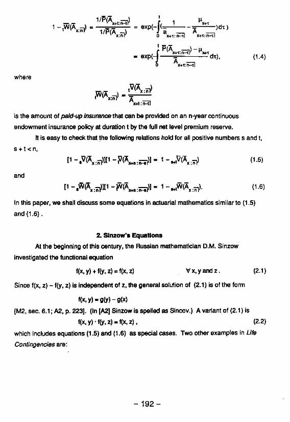
where

1/P(A ._\ I 1 - W(A _\ = x+l.rHY = ex (-J( 1

I x:nY 1/P(A) P a x: ii1 0 x+t: n:::tl

~x+t A )dt)

x+t:n=tl

I--

I P(Ax+'t:;;::::;tI) - ~lI+'t .. exp(- _ dt),

A o x+t:n::t1

IV(A _\ W(A _\ _ _ x:nY I x:nY A

X+l :n:il

is the amount of paid-up insurance that can be provided on an n-year continuous

endowment insurance policy at duration t by the full net level premium reserve.

(1.4)

It is easy to check that ~he following relations hold for all positive numbers sand t,

s +t < n,

(1.5)

and

[1 - W(A -\][1 - W(A _\] = 1 - W(A ) • x:nY ro X+I:~Y 1+1 x:;n· (1.6)

In this paper, we shall discuss some equations in actuarial mathematics similar to (1.5)

and (1.6).

2. Slnzow's Equations

At the beginning of this century, the Russian mathematician D.M. Sinzow

investigated the functional equation

f(x. y) + f(y, z) - f(x, z) V'x. yand z.

Since f(x, z) - f(y. z) is independent of z, the general solution of (2.1) is of the form

f(x. y) .. g(y) - g(x)

[M2, sec. 6.1; A2, p. 223]. (In (A2] Sinzow is spelled as Sincov.) A variant of (2.1) is

(2.1 )

f(x, y) • f(y. z) .. f(x, z) • (2.2)

which includes equations (1.5) and (1.6) as special cases. Two other examples in Ufe

Contingencies are:

-192 -

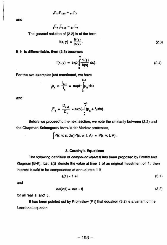
and

The general solution of (2.2) is of the form

h(y) f(x, y) - h(x).

If h is differentiable, then (2.3) becomes y

J h'(s) f(x, y) - exp( h(s) ds).

x

For the two examples just mentioned, we have

1 x+1

"'+1 J Px - T - exp(- ~. ds) x

and

D x+1

lEx - ~+I - exp(-J(~. + 3)ds). x x

(2.3)

(2.4)

Before we proceed to the next section, we note the similarity between (2.2) and

the Chapman-Kolmogorov formula for Markov processes,

Jp(r, v; s, dw)P(s, w; t, A) .. P(r, v; t, A) .

3. Cauchy's Equations

The following definition of compound interest has been proposed by Broffitt and

Klugman [B-1<]: Let a(t) denote the value at time t of an original Investment of 1; then

interest is said to be compounded at annual rate i if

a(1) II: 1 + i (3.1 )

and

8(S)8(t) - a(s + t) (3.2)

for all real s and t.

It has been pointed out by Promislow [P1] that equation (3.2) is a variant of the

functional equation

- 193-

f(s) + f(t) = f(s + t) , V s, t E R. (3.3)

Functional equations such as (3.3) and (3.2) had been studied by the eminent French

mathematician A.L. Cauchy (1821). Clearly, for each constant c the function

f(t) = ct (3.4)

is a solution of (3.3). Cauchy showed that, if the function f is continuous, (3.3) has no

other solution. In fact, the conclusion that (3.3) has no solutions other than those given by

(3.4) holds under anyone of the following weaker conditions: (i) f is continuous at a point;

(ii) f is bounded above in a neighbourhood of a point; (iii) f is bounded above on a set with

positive Lebesgue measure; (iv) there exists a set of positive measure on which f does

not take any value between two distinct numbers; (v) f is measurable in a neighbourhood

of a point; (vi) f is bounded above on a second category Baire set. On the other hand, it

. had been shown by G. Hamel and H. Lebesgue by transfinite induction that (3.3) has

infinitely many non measurable solutions. For expositions on (3.3), we refer the reader to

[A2; A3; Ei; R-V; Saa; Wi]. We note that equations (3.2) and (3.3) have appeared in

several of the Part 1 sample examinations released by the Society of Actuaries.

Now consider equation (3.2). Since a(t) .. [a(V2)]2, a(t) is nonnegative for all t. If

a(t) vanishes at some point to, then a(t) - a(t - to)a(to) - 0 for all t. By Broffitt and

Klugman's definition, a(O) .. 1. Thus, a(t) is strictly positive for all t. (We remark that, if

equation (3.2) were assumed to hold just for nonnegative t and s, then

{

1 taO a(t) - o t>O

would be a possible solution. However, (3.5) cannot be an accumulation function.)

(3.5)

The definition f(t) .. In a(t) transforms equation (3.2) into equation (3.3). Obviously,

the accumulation function a(t) has to be bounded above on each finite interval; thus by

(3.4) each solution of (3.2) is of the form

a(t) - act . (3.6)

Applying equation (3.1) yields

a(t) = (1 + ill • (3.7)

The constant c is ~, the force of interest. We note that formula (3.7) is derived from (3.2)

without any continuity assumption.

-194 -

Sinzow's equation (2.1) becomes Cauchy's equation (3.3) if f(x, y) is a function of

(y - x). Hence, Promislow [P2, sec. 2.3] has shown that an accumulation function a(s, t),

which is both Markov, i.e.,

a(r, s)a(s, t) = a(r, t), r< s <t,

and stationary, i.e., a(s, t) is a function of (t - s), must be of the form a(s, t) = ( 1 + i)l-s.

Other discussions on functional equations and compound interest can be found in [Lo;

Pe; Ei, sec. 1.5].

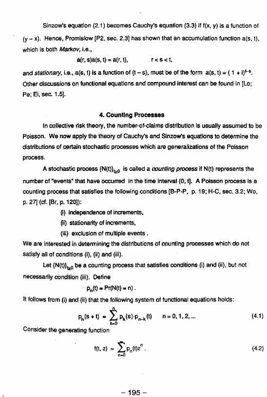
4. CounUng Processes

In collective risk theory, the number-ot-claims distribution is usually assumed to be

Poisson. We now apply the theory ot Cauchy's and Sinzow's equations to determine the

distributions of certain stochastic processes which are generalizations of the Poisson

process.

A stochastic process {N(t)}~o is called a counting process if N(t) represents the

number of "events" that have occurred in the time interval (0, t]. A Poisson process is a

counting process that satisfies the following conditions [B-P-P, p. 19; H-C, sec. 3.2; Wo,

p. 27] (ct. [Br, p. 120)):

0) independence of increments,

Oi) stationarity of increments,

(iii) exclusion of multiple events.

We are interested in determining the distributions of counting processes which do not

satisfy all of conditions (i), (ii) and (iii).

Let {N(t)}t;tO be a counting process that satisfies conditions (i) and (ii), but not

necessarily condition (iii). Define

Pn(t) - Pr(N(t) - n) .

It follows from (i) and (ii) that the following system of functional equations holds:

n

Pn(s+t) = LPk(S)'Pn-k(t) n=O,1,2, ... k-O

ConSider the generating function

f(t, z) = L Pn(t)zn . n..()

-195 -

(4.1 )

(4.2)

By (4.1)

f(s + t, z) = f(s, z) . f(t, z) .

Since f, as a function in its first variable, satisfies Cauchy's equation (3.2), there exists a

function h(z) such that f(t, z) = et II(z). In view of (4.2), put 2

h(z) = Ao + A1Z + ~z + ...

As f(t, 1) = 1, we have

Consequently,

f(t, z) '"' expHL A,> exp(t!: ~zj). (4.3) 1 1

Comparing the expansion of (4.3) in powers of z with (4.2), we obtain the formula

(4.4)

Put

Pn(t) ~ 0 for all n, it can be shown that A, ~ 0, i '"' 1, 2, 3, ....

Janossy, Renyi and Aczel [J-R-A] proved formula (4.4) by mathematical induction.

Their proof is repeated in the books [Sax] and [A2]. Formula (4.4) has been given in (lO].

In [Th], A, is denoted by Qj and Ais assumed to be 1.

If we write

. -1t t (A, t)T Xl(t) • e --

T 11

formula (4.4) becomes

- 196-

"4~O

Formula (4.5) implies the decomposition

N(t) • L jN;(t) , ;-1

(4.5)

(4.6)

where Nj(t) is a Poisson process with parameter ~. It can be proved that the Poisson

processes {N;(t)} are independent; see [peR] and [B-G-H-J-N, Theorem 11.2]. This result

is attributed to A.N. Kolmogorov [J-R-A, p. 211]. We remark that Feller [Fe, section XI1.2j

has shown that a distribution concentrated on the nonnegative integers is compound

Poisson if and only if it is infinitely divisible; an elegant proof of this fact by means of

recursive formulas has been given by Ospina and Gerber [O-G].

If the counting process {N(t)}~o also satisfies condition (iii), i.e., it is a Poisson

process, then ~ = ~ = A.4 = ... = a and (4.4) reduces to the usual formula

-At (A.t) n

Pn(t) = e n! (4.7)

On the other hand, if a counting process satisfies conditions (i) and (iii) but not the

stationarity condition (ii), we can use the technique of operational time to obtain a formula

similar to (4.7) [B-P-P, p. 353]. However, for a counting process satisfying only condition

(i), the method of operational time is not applicable; we now derive formulas which

generalize (4.4) and (4.5).

Let {N(t)}~o be a counting process which satisfies condition (i), but not

necessarily conditions (ii) and (iii). For s < t, N(t) - N(s) equals the number of events that

have occurred in the time interval (s, t]. Define

Pn(s, t) .. Pr(N(t) - N(s) = n) .

Then, for r < S < t and n = 0, 1, 2, ... , n

Pn(r, t) = L Pk(r, s)Pn-k(s, t) . k-O

-197 -

(4.1')

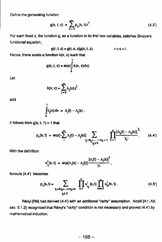
Define the generating function

g(s, t, z) = L Pn(s, t)zn. (4.2') n_O

For each fixed z, the function g, as a function in its first two variables, satisfies Sinzow's

functional equation,

g(r, t, z) - g(r, s, z)g(s, t, z),

Hence, there exists a function k(x, z) such that

Let

and

t

g(s, t, z) - exP(J k(x, z)dx) .

•

k(x, z) - !~(X)~ i-o

t

J~(X)dX" Aj(t)-Aj(S) .

• It follows from g(s, t, 1) .. 1 that

With the definition

[A.(t) - A.(S)]' xl (s, t) = exp[Aj(S) - Aj(t)] I I

Y 11

formula (4.4') becomes n _

r<s<t.

Pn(s,t)= L II xi (s, t) II x~(S, t) . 1-1 ~ i-n+1 y,+2'r2+ .. ·+nyn-n

l~o

(4.5')

R~nyi [R~] had derived (4.4') with an additional RrarityR assumption. Acz~1 [A1; A2,

sec. 5.1.2] recognized that R~nyi's RrarityR condition is not necessary and proved (4.4') by

mathematical induction.

- 198-

j

I I

We conclude this section with a remark on stochastic processes (not necessarily

counting processes) which have independent and stationary increments. Let {X(t)} be

such a stochastic process with X(O) .. O. For 0 < S < t.

~t. 9) = E{exp(i9X(t)]}

= E{exp(i9(X(t) - Xes) + Xes»)]}

= E{exp(i9(X(t) - Xes»)]} E{exp[i9X(s)]}

- E{exp(i9(X(t - s»)]} E{exp[i9X(s)]}

- ~t - s. 8) «s. 9) .

Since 4». as a function in its first variable. satisfies Cauchy's equation (3.2). we have

~t. 8) _ [~1. 9))1

under mild assumptions. The branch of the multivalued function log[4»(1. 9)] with

109[4»(1. 0)] .. 0 is called the cumulant generating function per unit time and had been

shown by Kolmogorov [Cr. chapter 8; Se] to be of the form

(4.8)

where K(x) is a bounded and nondecreasing function continuous at x .. O. Formula (4.8)

can be expressed in another way. known as the Levy-Khintchine canonical form. Cf. [Ta.

Appendix 3].

5. interpolation Theory

Recall the translation operator E in Finite Differences,

E'f(x) - f(x + t) .

It is easy to see that the following operator equation holds:

E' E' = es+1• (5.1 )

As equl'ltion (5.1) is similar to (3.2). one may wonder if there is an equation analogous to

(3.6). If D denotes the differentiation operator. the Taylor expansion formula may be

written symbolically as

(5.2)

- 199-

Hence, we have [Fr, p. 126] f:t _ etD•

For a rigorous functional analytic treatment of the operator equation (5.2'), see [H-P,

chapter 19] or [Yo, sec. IX.51 .

We remark that formula (5.2') can be generalized to higher dimensions. For

f: R" ~ R, define

~ f(x) ,. f(x + t) ,

where t .. (t1' ... , tn)T and x - (X1' ...• xn)T. Then [Fr. p. 141; M1. p. 109]

t,~+ •.. +t,,~ Et , -.."

- e

t . ..L ~.

- e

where ~ is the gradient operator (!- ..... -t-{ aX a~ ~"

Recall the Newton forward-differenc9 and backward-difference formulas:

(5.2')

Et ,. (1 + A)t ... !, (~)t} (5.3) 1-0 I

and

(5.4)

For j = O. 1. 2 •...• define [S1 • p. 8]

m j j j t - t(t+2'-1)(t+2'-2) ... (t-2'+1).

Then,

t ta lJl . E.. ~. _0 J

(5.5)

where ~ is the central-differenc8 operator. In examining formulas (5.2). (5.3), (5.4) and

(5.5). one would feel that there should be a general theory behind these expansions.

Consider the linear space of polynomials. A linear operator on this space is called

translation invariant.if it commutes with the translation operator E. Each translation­

invariant operator can be expressed as a power series in 0 [Ga, Theorem 1.1]. A

translation-invariant operator of the form

- 200-

c1 "'0. (5.6)

is called a delta operator [M-R. p. 180]. Obvious examples of delta operators are D.!J. (=

eO - I). V (= I - e-O ) and l) (= eD12 - e-012). We note that. since c1 '" O. it follows from the

Lagrange inversion fonnula (1768) that we can invert (5.6) and express the differentiation

operator 0 as a power series in 0 [Ga, Lemma 1.1; Kn, p. 508].

J.F. Steffensen [S3], the late Professor of Actuarial Science at the University of

Copenhagen, observed that, for each delta operator 0, there is a unique sequence of

polynomials qo(t) ;;; 1, q1(t), q2(t), ... such that qj(t) is a polynomial of degree j,

o • q1 (0) = ~(O) .... . and, for j = 1, 2, 3, ... ,

Qqj(t) .. jqj-1 (t).

Steffensen called these polynomials poweroids. Since the sequence of polynomials

{qj(t)} forms a basis for the linear space of all polynomials and

k I {jl k = j Oqj(t)t_o= 0 k"'i'

we have the following generalization of the Taylor expansion fonnula:

Et 600 qj(t) d·

.. '1 . J- J

It follows from (5.1) and (5.8) that, for i = 0, 1, 2, ... and s, t e R,

qj(s + t) .. t qk(S) qj-k(t)

il t:fJ kl 0 - k)1

or

qj(s + t) = ~ 0) qk(S)qj-k(t) .

Note the similarity between the systems of functional equations (5.9) and (4.1). In the

speCial case where qj(t) = t(t-1 )(t-2) ... (t-j+ 1 ),

(5.9) is known as Vandermonde's Theorem.

- 201 -

(5.7)

(5.8)

(5.9)

Formula (5.9) generalizes the binomial theorem and was first observed by

Steffensen [53, sec. 13). Three decades later, R. Mullin and G.-C. Rota [M-R, Theorem

1 b] showed that the converse is also true: A sequence of polynomials, one for each

degree and satisfying the binomial identity (5.9) tor all j, sand t, must be the poweroids of

a delta operator.

Remarks. (1) Recall the Z-msthod in Ufe Contingencies [Jo, sec. 10.3), where subscripts

are treated as exponents. 5imilarly, equation (5.9) can be written umbral/y as

q(s + tV • [q(s) + q(t)P .

For a recent exposition on the umbral calculus, see the book [Ro).

(2) Consider the delta operator b

O eae-I 1ea . .. ---- fl. . b b b'

it can easily be shown [52; 53, p. 346] that its poweroids are ~(t) • 1 and, for i = 1, 2, ... ,

qj(t) = t E-fa(t - b)(t - 2b) ... (t - (j-1 )b)

.. t(t - ja - b)(t - ia - 2b) .•. (t - ia - (j-1)b).

This formulation includes as special cases the delta operators fl., V, S and 0 (b -+ 0).

We now conclude this paper with a derivation of some classical formulas in

interpolation theory. Since E' .. etD, differentiating (5.8) with respect to 0 yields [53, (32)]

Et. t qt+1(t) d dO (5.10) ~ til dO'

Now, consider 0 = Sand qj(t) .. tID. Writing t[j]/t as tliJ-1 and noting that 112 -1e

~ .. ~E'12 _E-112) = E + E "" Il

dO dO 2

(which is the averaging operator), we have [53, (147)] - D+1}-1

t ~ t . E _ ~_jl_j.LSJ. (5.11 )

Comparing (5.8) and (5.10). one may conjecture the formula [53, (15); M-R.

Theorem 4.4]:

- 202-

Also, putting T = dO/dD, we can rewrite (S.10) as -1

I ~ T qj(t) d· E = ~ ., T,

1- 0 J (S.12)

which is in fact valid for all invertible translation-invariant operators T [R-K-O, section S].

Formulas (S.S) and (S.11) are not useful for interpolation as they require values at

-o.S, O.S, 1.S, ... etc., in addition to values at integral points. However, by splitting these

two formulas into their odd and even components, we can easily derive the classical

central-difference interpolation formulas. Indeed, the Gauss forward and backward,

Everett and Steffensen formulas are immediate consequence of the odd-even

decomposition of (S.11).

For j = 1, 2, 3, ... , / ·-1

tr<!il = fi (l- k2

)

!.! and

j-1 r<!i+1] J] 2 1 2"

t = t [t - (k +"2) J ; -0

hence {t[2il} and {t[2i+1}-1} are even functions and {t£2H~ and {t£2il-1} are odd functions.

Therefore,

(S.13)

and I 4 - r<!i-1] - r<!il-1

E -E ~ t 2H "'" t 2H 2 = ~ (2· _1),5 = ~ (2· -1)1 ~5 .

1-1 J 1- 1 J (S.14)

(Observing that 5 = eD12 - e-012 is an odd function in D, we see that formulas (S.13) and

(S.14) can be generalized. Consider 0 = g(O); then

elg-'(Q) = e lD = EI = ! q~t) d. j-O jl

If g is an odd function, its inverse g-1 is also an odd function; hence {q2j(t)} and {q2j+1(t)lt}

are even polynomials, and (q2H(t)} and {q2j(t)lt} are odd polynomials.)

- 203-

Combining (5.13) and (5.14), we obtain the Stirling and Bessel interpolation

formulas: .. 12il 12j+2}-1

t ~ t 2j t 2j+1 E = ~ 2jl 0 + (2j + 1)! JlO ,

.. 12j+ 1}-1 12i+ 1] t ~ t 2j t 2i+1

E = ~2JIJlO + (2j + 1)1 0 .

To derive the Everett formula, note that t E _ E-1 t Et _ E-t E 1-t _ E-(1-1)

E = -1 E = -1 E + ----::--E-E E-E E_E-

1

and

EX _E-x

EX _E-x ~ lj}-1 tj-2 ~ .. (X+k) 2k

E_E-1 = = ~(2·-1)1 =2k+1 0 . 2J.10 ).1 J. k.

To obtain the Steffensen formula, consider

Using the formula X -x

E +E 2

.. 12j+1}-1 ~x 2j

= Jl + £..J 2·' JlO, j.1 )

we get

To derive the Gauss forward and backward formulas we employ the following

odd-even decompositions: t -t Et-11l + E-(t-112)

t E - E 112 E = E112 + E-112 E + E'12 + E-112

and

Et= t -t Et + 112 + E-(t+ 112) E - E -112

112 -112 E + 112 -112 E +E E +E

- 204-

The odd component of (5.5),

Et E-I - 12i+1) - ~ t 2t+1

2 = i~ (2j + 1)1 S .

can be used to give a simple derivation of the "summation n" formula and King's

pivotal-value formula in Graduation Theory. The operator "summation n" is defined by nI2 -nI2

[] E(n-1)12 E(n-3)12 E-{n-1)12 E - E

n = + + •.• + = 112 -112 . E -E

Thus, nI2 -nI2 - 12t+1) 2 2 2 2

[] = E -E .. 2~ (n/2) ~2i = n(n -1)s2 n(n -1)(n -3 )~4 n S ~ (2j+1)1 0 n+ 24 + 1920 u + ...

King's formula is obtained by inverting the "summation n" operator: 112 -112 E112n _ E -112n

-1 E - E n n [n] = nI2 -nI2 = S

E -E n - 12t+1] - 12t+1H

= 2) (1/2n) S2i = .!.) (112n) tfi ~ (2j+1)1 n n~ (2j+1)1 n 222

(5.15)

= 1. _ ~S2 + (n -1)[(3n) -1] S4

n 24n3

n 1920n5

n (5.16)

It had been observed by G.J. Udstone [1l1 that the coefficients in (5.16) can be obtained

from those in (5.15) by substituting 1/n for n. Hence, we have the "formula"

[nJ1 .. [n-1].

Acknowledgment

I began writing this paper when I was on sabbatical leave at the University of

Michigan several years ago. I wish to take this opportunity to thank Professor and Mrs.

Nesbitt for their hospitality.

References

[A1] J. Aczel, "On Composed Poisson Distributions, III," Acta Mathematica Academiae

Scientiarum Hungaricae, 3 (1952), 219-223.

[A2] J. Aczel, Lectures on Functional Equations and Their Applications. New York:

Academic Press, 1966.

- 205-

[A3] J. Aczel, On Applications and Theory of Functional Equations, Basel: Birkhauser

Verlag and New York: Academic Press, 1969.

[B-P-P] R.E. Beard, T. Pentikainen and E. Pesonen, Risk Theory: The Stochastic Basis of

Insurance, 3rd ed., London: Chapman and Hall, 1984.

[Be] A. Berger, -Ober den Einfluss einer Anderung der Sterblichkeit auf die

Pramienraserve: Skandinavisk Aktuarietidskrift, 19 (1936), 52-54 .

[B-G-H-J-N] N.L Bowers, Jr., H.U. Gerber, J.C. Hickman, D.A. Jones and C.J. Nesbitt,

Actuarial Mathematics, Itasca, IL: Society of Actuaries, 1986.

[B-H-N] N.L Bowers, Jr., J.C. Hickman and C.J. Nesbitt, -Notes on the Dynamics of

Pension Funding,- ARCH, 1981.1,21-38. Reprinted in Insurance: Mathematics

and Eoonomics, 1 (1982),261-270.

[B-1<] J.D. Broffitt and S. Klugman, -~finitions for Compound and Simple Interast,­

ARCH, 1982.2, 3-4; The Actuaf)', January 1983, 7.

[Br] T.C. Brown, -Poisson Approximations and the ~finition of the Poisson Process,­

American Mathematical Monthly, 91 (1984),116-120.

[Cr] H. Cramer, Random Variables and Probability Distributions, 3rd ed., London:

Cambridge University Prass, 1970.

[Ei] W. Eichhorn, Functional Equations in Eoonomics, Reading, MA: Addison- Wesley,

1978.

[Fe] W. Feller, An Introduction to Probability Theory and Its Applications, Vol. 1, 3rd ed.,

New York: Wiley, 1968.

[Fr] H. Freeman, Finite Differences for Actuarial Students, London: Cambridge

University Press, 1960.

[Ga] A.M. Garsia, -An Expose of the Mullin-Rota Theory of Polynomials of Binomial

Type,- UfJ8ar and Multilinear Algebra, 1 (1973),47-65.

[H-PJ E. Hille and R.S. Phillips, Functional Analysis and Semi-Groups, rav. ed., Rhode

Island: American Mathematical Society, 1957.

[H-C] R.V. Hogg and A.T. Craig, Introduction to Mathematical Statistics, 4th ed., New

York: Macmillan, 1978.

[J-R-A] L. Janossy, A. Renyi and A. Aczel, -On Composed Poisson Distributions, 1,- Acta

Mathematica Academiae Scientiarum Hungaricae, 1 (1950), 209-224.

[Jo] C.w. Jordan, Jr., Ute Contingencies, 2nd ed., Chicago: Society of Actuaries, 1967.

- 206-

I , I

; \,

: ~ ! j I ~

\

,

I I

I

I

\~ ) II )

r I

~

, f !

) 'I

I J

[K-U)

[Kn]

[Le]

[Li]

[Lo)

[LO]

[M1]

[M2]

[M-R]

[o-G]

[Pel

[P1]

[P2]

[P-R]

[Re]

D. Kalman and A. Ungar, wCombinatorial and Functional Identities in One­

Parameter Matrices,w American Mathematical Monthly, 94 (1987),21-35.

D.E. Knuth, The Art of Computer Programming, Vol. 2 Seminumerical Algorithms,

2nd ed., Reading, MA: Addison-Wesley, 1981.

G. Letac, WCauchy Functional Equation Again," American Mathematical Monthly,

85 (1978), 663-664.

G.J. Lidstone, wGeneral Relations between Central Sums and Central Terms,"

Journal of the Institute of Actuaries, 55 (1924), 177-180.

A. Loewy, "Axiomatische BegrOndung der Zinstheorie," Jahresbericht der

Deutschen Mathematiker-Vereinigung, 26 (1919), 26-31.

R. LOders, "Die Statistikderseltenen Ereignisse," Biometrika, 26 (1934),108-128.

Z.A. Melzak, Companion to Concrete Mathematics: Mathematical Techniques and

Various Applications, New York: Wiley, 1973.

Z.A. Melzak, Mathematical Ideas, Modeling and Applications: Volume /I of

Companion to Concrete Mathematics, New York: Wiley, 1976.

R. Mullin and G.-C. Rota, "On the Foundations of Combinatorial Theory III, Theory

of Binomial Enumeration," Graph Theory and Its Applications, edited by B. Harris,

New York: Academic Press, 1970, 167-213.

A.V. Ospina and H.U. Gerber, "A Simple Proof of Feller's Characterization of the

Compound Poisson Distributions," Insurance: Mathematics and Economics, 6

(1987), 63-64.

J. Pepis, "Sur une famille d'ensembles plans et les solutions de I'equation

fonctionnelle F(x, z) = F(x, Y)'F(y, z) pour 0 ~ x ~ y ~ z. Application a la tMorie

generale des inten~ts," Annales de la Societe Polonaise de MatMmatique, 17

(1938), 113-114.

S.D. Promislow, WTheory of Interest," A Letter to the Editor of The Actuary, March

1983,2.

S.D. Promislow, "Accumulation Functions," ARCH, 1985.1,39-56.

A. Prekopa and A. Renyi, "On the Independence in the Limit of Sums Depending

on the Same Sequence of Independent Random Variables,w Acta Mathematica

Academiae Scientiarum Hungaricae, 7 (1956), 319-326.

A. Renyi, "On Composed Poisson Distributions, H,w Acta Mathematica Academiae

SCientiarum Hungaricae, 2 (1951), 83-98.

- 207-

[R-V] A.W. Roberts and D.E. Varberg, Convex Functions, New York: Academic Press,

1973.

[Ro] S. Roman, The Umbral Calculus, New York: Academic Press, 1984.

[R-K-O] G.-C. Rota, D. Kahaner and A. Odlyzko, ·On the Foundations of Combinatorial

Theory VIII, Finite Operator Calculus,· Journal of MathematiCal Analysis and

Applications, 42 (1973),685-760. Reprinted in G.-C. Rota, Finite Operator

Calculus, New York: Academic Press, 1975, 7-82.

[Saa] T.L. Saaty, Modem Nonlinear Equations, rev. ed., New York: Dover, 1981.

[Sax] W. Saxer, VelSicherungsmathematikerll, Berlin: Springer-Verlag, 1958.

[Se] C.O. Segerdahl, -On the Probability Function of a Homogeneous Random

Process,- Skandinavislc AJctuarietidskrift, 1969, 163-174.

[Sh] E.S.W. Shiu, -Steffensen's Poweroids,- Scandinavian Actuarial Journal, 1982,

123-128.

[S1] J.F. Steffensen, Interpolation, Baltimore: Williams and Wilkins, 1927. Reprinted by

Chelsea, New York, 1950.

[S2] J.F. Steffensen, -On the Definition of the Central Factorial,- Journal of the Institute

of Actuaries, 64 (1933), 165-168.

[S3] J.F. Steffensen, ~e Poweroid, an Extension of the Mathematical Notion of

Power,- Acta Mathematica, 73 (1941), 333-366.

[Ta] L Takacs, Combinatorial Methods in the Theory of Stochastic Processes, New

York: Wiley, 1967. Reprinted by Krieger, Huntington, NY, 1977.

[Th] P. Thyrion, -Extension of the Collective Risk Theory,- The Filip Lundberg

Symposium, Section IX of the Supplement toSlcandinavisk Aktuarietidskrift, 52

(1969), 84-98.

[Va] P. Vasmoen, -Ober den Einfluss einer Anderung der Sterblichkeit auf die

PrAmienreserve und andere damit verwandten Fragen, - S1candnavisk

Aktuarieticiskrift, 18 (1935), 1-34. Also see [Be].

[Wi] A. Wilansky, -Additive Functions,- Lectures on Calculus, edited by K.O. May, San

Francisco: Holden-Day, 1967,95-124.

[Wo] J.C. Wooddy, Risk Theory, Part 5 Study Note 55.1.71, Chicago: Society of

Actuaries, 1 ~73.

[Yo] K. Yosida, Functional Analysis, 4th ed., New York: Springer-Verlag, 1974.

- 208-