Some elementary statistical and numerical procedures—An interactive approach

Compuf & Educomn. Vol 2, pp 145-I 76 0 Pergamon Press Ltd 197s Prmed in Great Bntam

SOME ELEMENTARY STATISTICAL AND NUMERICAL PROCEDURES-AN INTERACTIVE APPROACH

J. D. LEE and D. G. HAYES

Department of Chemistry. Loughborough University of Technology, England

GETTING STARTED

When setting up a computer laboratory to provide interactive facilities for general scientific use, the first requirement, after obtaining access to a computer and a terminal, is a set of small computer programs to perform common routine calculations. In the following section several very thoroughly tested programs are described. These will:

1. calculate the area under a curve; 2. calculate the standard deviation of a set of readings; 3. fit the best straight line to a set of graph points; 4. fit a polynomial to a set of graph points; 5. perform the chi-squared statistical test; 6. perform the r and I; statistical tests.

SOME PRIMARY OBJECTIVES

By using programs such as the ones described, users obtain results which are more accurate than are obtained by plotting graphs or measuring areas by hand. In addition, the results from the computer are reproducible. Furthermore, an increased awareness of the meaning of numbers and the accuracy of

results calculated from experimental data grows on many users. The more dedicated users look at the program itself and become familiar not only with the mathematical method but also with com- puting methods and programming.

GENERAL POINTS ABOUT THE PROGRAMS

The programs are all completely self contained, and print sufficient instructions to allow an absolute beginner to perform the chosen calculation without needing to refer to an instruction manual or a laboratory sheet. Printing out long explanations becomes tedious and time wasting once a user has become familiar with the program, so at the beginning of each program the user is asked whether he would like full instructions or not. Depending on the reply either full instructions or the minimum of short instructions are printed. After a run, users are asked if they wish to finish or have another run, and in the latter case they are expected to have learnt how to use the program so only short instructions are printed on the second or subsequent runs.

To aid transportability of the programs from one computer to another, the programs described have been written in STANDARD FORTRAN IV and conform to the ANSI standard X 3.9 dated March 1966. The programs have been tested using several compilers including ICL (XFAT), South- ampton University (SOFOR) and CDC 7600 (FTN).

A major drawback of standard FORTRAN is that it does not allow the use of FREE FORMAT for the input of data values. FREE FORMAT has great advantages when using a terminal, since the exact number of digits making up any particular number is of no importance. Even more important, when two numbers are input in one line they need only be separated by a space, rather than arranged in particular columns. Not all compilers allow the use of FREE FORMAT, and the method of implementation is specific to the particular computer used, but for guidance the input FORMAT statements which could be used on ICL 1900 series computers are included as comment cards next to the FORMAT statements actually used in the programs.

Terminal programs should be robust, and should not fail (or even worse give incorrect results) because of an unfortunate combination of data, or completely erroneous or incomplete data. This may arise because of the lack of expertise of a novice or even deliberate sabotage! As far as is practic- able, these programs check the input data. If the user is asked to type 0 or 1 for two options, the program checks that some other number has not been typed, and if necessary requests that the choice

145

146 J. D. LEE and D. G. HAYES

be made correctly. In the course of calculations division by zero is iatal, and checks are made to prevent this. However any program will fail if numbers outside the range,which the particular computer can handle are input as data or produced in calculations, or if letters are input when numbers are expected.

The programs all require a number of data values to be typed in, whether for a straight line fit by least squares or calculation of the standard deviation etc. The number of data values will vary from one run to another, and by experience it has been found preferable to make the computer count the number of terms rather than asking the user. This is accomplished by typing a dummy value of999999. which is recognised by the computer as the terminator, and hence the end of rhe data. It should be noted that each data value is read in and checked to see if it is the terminator. In principle testing if two real numbers are exactly equal is dangerous since rounding off errors when converting the numbers into binary form in the computer could result in two identical numbers appearing to be different. This has not happened on any machine tested so far, but should users encounter this difficulty they should change the terminator to some other number.

Many terminal systems do not recognise all of the lineprinter control characters (1 H 1, 1 HO, I H , 1 H+ ), and so the spacing of printed lines of output is achieved using only the solidus i and the control character 1 H , which are universally available.

In all cases a sample run is provided to illustrate the use of the particular program, and to provide trial data for others implementing the program.

CALCULATION OF THE AREA UNDER A CURVE

IntroJuction

A problem in determining the areas of peaks from chart recorder output often arises in U.V. spectro- photometry, gas chromatography and other similar techniques. Areas are commonly measured by tesselation (counting squares), planimetry, or by cutting out and weighing the paper. These methods have disadvantages-they are tedious, inaccurate, and the last method destroys the original trace. Some gas chromatographs have built in integrators to measure peak areas, but the computer program described below is applicable to any curve for which suitable coordinates can be measured.

Area is a computer program which calculates the area under a curve using Simpson’s rule. The height of the curve must be given at equal intervals along the .X axis, and an odd number of data points is

required.

Background

The most common methodofcalculating the area under a curve give the y coordinates y,, yZ, Ye, y4, _. at equal intervals along x involves fitting a polynomial through n points at a time, and subsequently integrating the polynomial. Consider taking two points from a curve (n = 2).

There must be more data points than there are variables in the equation, or the result- will be indeterminate. The maximum order of the polynomial is therefore II - 1 = 1. corresponding to a straight line 0’ = al + b). The curve fitting therefore corresponds to drawing a straight line between the two points, producing a trapezium. The area of this can be calculated geometrically f: sum of parallel sides x distance between them). If this process is repeated with subsequent pairs of points the total area under the curve is obtained from the sum of the areas of all the trapezia. This is known as the trapezium rule.

Now consider fitting a curve to three points (n = 3), allowmg a maximum order of the polynomial of n - 1 = 2. that is a quadratic equation _Y = ax2 + bx + c. This corresponds to fitting a curve

Some elementary statistical and numerical procedures-an interactive approach 147

through the first three points. The area under the first quadratic may be calculated.

)‘3

Y, f(x). dx = ;. Ax . (y, + 4y2 + y3).

Then a quadratic function is fitted to points 3, 4 and 5. The total area under the curve is the sum of the areas under each quadratic. This method is known as Simpson’s rule, and should give a more accurate result than trapezium rule since drawing a curve is likely to give a better estimate of the area than drawing straight lines. Simpson’s rule imposes one condition-there must be 3, 5, 7,. . or generally any odd number of data points present. This rule may be adapted for automatic work since the value of the integral is the sum of the lirst and last y values plus twice the sum of the other odd y values plus four times the sum of all the even y terms, all multiplied by one third of the distance between the x values.

Ax area = 1. (y, + 2X other odd y values + 4X even y values + last y).

In principle the use of a higher order polynomial such as cubic (order = 3) corresponding to fitting a curve through four points at a time might give a smoother curve through the points. However, high order polynomials sometimes produce unwanted spikes in the curve, and are generally avoided. For most purposes, the best results are obtained using Simpson’s rule with a fairly small interval along the x axis.

Description of the program

The program first prints a heading, asks if full instructions are required, and then invites the user to type in the interval between the readings on the x axis. A check is performed to ensure that the interval is greater than zero. Next a message requests that the y coordinates of the data points be typed in one at a time. The first value is stored, and the sum of the odd numbered y values, and the sum of the even numbered y values are collected for later use. The number of points is also counted. A dummy value of 999999. is typed to signal the end of the data. The y values must be measured at equal intervals along x, but the actual numerical values of x are not required since the area under the curve remains the same even if the curve is moved to the left or right. Up to one thousand y values may be typed in.

A test is performed to make sure that there are at least three data points before starting the calculation. If there are not, then the run is terminated with a message that there are not enough data points.

Then a check is made to see if an odd number of data points has been provided, since this is a pre- requisite for Simpson’s rule. If an even number of points has inadvertently been provided, a message is printed explaining this, and inviting the user to choose between two alternatives. These are either to ignore the last data point and use Simpson’s rule on the remainder of the points, or alternatively to calculate the area by Simpson’s rule as in the first option and then to calculate the area for the last segment by the trapezium rule, and add the two together.

Finally the area is printed. followed by a message asking whether the user would like another run with new data, or wishes to finish. At the end a message is printed that the job has been completed successfully.

FORMAT statements 3 and 9 should be changed to FREE FORMAT if possible.

148 J.D. LEE and D.G. HAYES

Listing of AREA program

WRITE(2,l) 1 FORMAT(//52H CALCULATION OF AREA UNDER A 1 52~ ___________ __ ____ ___________ __ ____ ===== =

CURVE BY SIHPSONS RULE./ ____e __ _____ __ ===I==== ==.zs//

2 34H WOULD YOU LIKE FULL INSTRUCTIONS?/ 46H TYPE 1 FOR YES, OR 0 FOR NO. THEN PRESS RETURN.)

23READ(1.3J INSTR 3

C C 3

4

5 6

: 9

C c 9

:0 11

12

13

14

C C

15

: C

16

FORHAT(I1) IF POSSIBLE THE ABOVE FORMAT SHOULD BE REPLACED BY FREE FORMAT FORMAT(I0) IF(INSTR.EP.O.OR.INSTR.EO.1) GO TO 5 WRITE(2,4) FORMAT(/17H RETYPE CORRECTLY) GO TO 2 WRITE(2,6) FORMAT(/52H TYPE IN THE INTERVAL BETWEEN READINGS ON THE X AXIS) IF(INSTR.EO.1) WRITE(2.7) FORMAT(~~H THEN PRESS RETURN./) READ(1.9) X FORHAT~F10.0) IF POSSIBLE THE ABOVE FORMAT SHOULD BE REPLACED BY FREE FORMAT FORMAT(FO.0) IF(X.GT.O.0) GO TO 10 WRITE(2,4) GO TO 8 IF(INSTR.EQ.1) WRITE(2,11) FORMAT(/34H TYPE Y VALUE OF FIRST DATA POINT.1 1 48H THEN PRESS RETURN AND TYPE THE NEXT DATA POINT./ 2 44H THERE MUST BE AN ODD NUMBER OF DATA POINTS./ 3 39H TERMINATE DATA WITH A VALUE OF 999999./j IF(INSTR.EQ.0) WRITE(2,12) FORHAT(/14H TYPE Y VALUES/) IEV=O SUMHOD=O.O SUUHEVaO.0 DO 14 X=1,1000 READ(1,9) H IF(H.EG.999999.) GO TO 15 N-1 IF(I.EO.l) Hl=H IF(I/2*2.NE.I) GO TO 13 HEV=H _ SUMHEV=SUHHEV+H GO TO 14 HOD=H SUMHOD=SUMHOD+H CONTINUE

TEST THAT THERE ARE ENOUGH DATA POINTS IF(N.LT.3) GO TO 21

TEST THAT AN ODD NUMBER OF DATA POINTS HAS BEEN GIVEN AND DECIDE WHAT TO DO IF NUMBER IS EVEN. IF(2*(N/2).NE.N) GO TO 19 WRITE(2,16) FORHAT(/45H AN EVEN NUMBER OF DATA POINTS HAS BEEN GIVEN/ 1 46H TYPE 0 IF THE LAST VALUE IS TO BE IGNORED, OR/ 2 49H TYPE 1 IF THE LAST VALUE IS TO BE INCLUDED USING/ 3 20H THE TRAPEZIUM RULE.) mIF(INSTR.EP.l) WRITE(2,7)

17 READ(1,3) IEV IF(IEV.EO.O.OR.IEV.Ec,l) GO TO 18 WRITE(2.4) GO TO 17

C C WORK OUT AREA

18 SUMHEVnSUMHEV-HEV TRAPEZ=(HEV+HOD)/2.0*X

19 SUMHOD=SUMHOD-Hl-HOD AREA=(X/3.0)*(H1+2.0*SUMHOD+4.O*SUMHEV+HOD~ IF(IEV.EO.l) AREA=AREA+TRAPEZ WRITE(2.20) AREA

20 FORMAT(/lgH AREA UNDER CURVE =,lPE11.4) GO TO 23


c C ENTER IF ERRORS FOUND

21 WRITE (2,221 22 FORMAT(140H RUN ABANDONED - NOT ENOUGH DATA POINTS.)

23 WRITE(2,24) 24 FORMAT(/38H TYPE 1 FOR ANOTHER RUN OR 0 TO FINISH/)

IF(INSTR.EQ.1) WRITE(2,7) 25 READfl,3f IEND

IFfIEND.EO.0) GO TO 26 INSTR=O IF(IEND.EO.1) GO TO 5 WRITEf2,4) GO TO 25

c C TERMINATE JOB

26 WRITE(2,27) 27 FORHAT(128H JOB COMPLETED SUCCESSFULLY./)

STOP END

Trial rug with AREA program

CALCULATION OF AREA UNDER A CURVE BY SIMPSONS RULE. =tD=======' I= =5== rr=== : _____ __ ___*_*__ I:=:= --___ __ ____----

WOULD YOU LIKE FULL INSTRUCTIONS? TYPE 1 FOR YES, OR 0 FOR NO. THEN PRESS RETURN. ?l

TYPE IN THE INTERVAL BETWEEN READINGS ON THE X AXIS THEN PRESS RETURN. ? .5

TYPE Y VALUE OF FIRST DATA POINT. THEN PRESS RETURN AND TYPE THE NEXT DATA POINT. THERE MUST BE AN ODD NUMBER OF DATA POINTS. TERMINATE DATA WITH A VALUE OF 999999. ? 16. ? 8. ? 4. ? 2.

; h9999.

AREA UNDER CURVE = l.O833E+Ol

TYPE 1 FOR ANOTHER RUN OR 0 TO FINISH

THEN PRESS RETURN. ?O

JOB COMPLETED SUCCESSFULLY.


STANDARD DEVIATION AND CONFIDENCE LIMITS

Introduction

Standard deviation is a computer program which calculates the mean of a series of numbers, the standard deviation, and optionally the 95 and 99 o/0 confidence limits. The 95 O’, confidence limits are defined as being two numbers with the following property: The mean of the population from which the sample numbers were chosen has a 95 “i, chance of lying between the confidence limits.


Firstly a heading is typed out, the user is asked if full instructions are required, then a message invites the user to type in the data values one at a time. These numbers are stored in an array which may hold up to 500 values, and the number of terms is counted. The end of the input data is indicated by typing a dummy value of 999999.. If 500 data values have been typed in before the terminator has been encountered, a warning message is printed stating that the program can only handle 500 values, and the calculations continue on the data already entered. If less than two data terms are entered before the terminator, a message is typed that the attempt to run with this data is abandoned because there are insufficient data points. The user may then choose either to type in a new set of data, or to terminate the job altogether.

The program next works out themean value

AV = C data values/number of terms

and then calculates SIGMA the standard deviation. If there are less than thirty data values, the expression used is :

SIGMA = Z (data value - average value)’

(number of terms - 1

If there are thirty or more data values the denominator in the above equation is replaced by the number of terms. The number of readings. the average value, and the standard deviation are printed out.

A message then asks the user to type 1 if confidence limits are required, or 0 to bypass this calculation. For a finite number of observations, n, the confidence limits are given by

confidence limit = AV + -!- SIGMA \’ n

where AV is the mean value, SIGMA is the standard deviation and t a quantity from statistics theory

which varies with n [l]. Values of t/,/n for values of n from 2 to 20 are stored in arrays, and the

appropriate values are used to evaluate the 95 % and the 99 7; confidence limits. For cases where there are more than 20 readings an approximation is used to calculate t:

f = ,,/:.sinh bJ(&$_--1

where v is the number of degrees of freedom (n - 1) and T has the value I.960 for the 95 3’, confidence limit and 2.576 for the 99% confidence limit. Since FORTRAN does not contain a function for hyperbolic sines, this term is evaluated

sinh x = qeX - e-“). 2

The confidence limits are then printed out. The next message invites the user to type 1 for another run with a new set of data. or 0 to finish

the job. At the end of the job a finishing message is printed. Format statements numbers 5 and 9 should be changed to FREE FORMAT if possible.


Listing of STANDARD DEVIATiONprogram

20),T99(20) 5(3),~95(4),T95(5),T95(6),T95(7),T95(8), 1).~95(l2),T95(13),T95(14),T95(15),T95(16)v

DIMENSION A(5GO),T95(, DATA T95(1),T95(2),T9' 1 T95(9I,T95(1O),T95(1 2 T95(17),T95(18),T95(19) 3 /0.0,8.984,2.484 4 0.715,0.672,0.635,0.604 DATA T99(?),T99(2),T99(? 1 T99(9),T99(10),T99(11), 2 T99(l?),T99(18),T99(~9) 3 10.0.45.0.5.?10. 4 1.028,0.955

.241,1 1.554 ,o ,T99(5 T99( 13

925,0.836,0.769, 514,o.497,0.482,.468/ l),T99f?),T99(8), 4),T99(15),T99(16),

PRINT TITLE WRITE (2.1)

1 FORMAT(//JlH STANDARD DEVIATION CALCULATION/ 31H =Z:=ZS=E

2'WRITE(2 3) :=:====3= =.=I=..====/)

3 FORNAT(j4H WOULD YOU LIKE FULL INSTRUCTIONS?/ 1 28~ TYPE 1 FOR YES OR 0 FOR NO.) WRITE(2,4) FORMAT(l9H THEN PRESS RETURN.) READ(1,5) INSTR FORMAT(I1) IF POSSIBLE THE ABOVE FORMAT SHOULD BE REPLACED BY FREE FORMAT FORMAT(I0) IF(INSTR.E~.O) GO TO 7 IF(INSTR.NE.1) GO TO 2 WRITE(2,6) FORMAT(I35H TYPE IN DATA VALUES ONE AT A TIME./

: 30H PRESS RETURN AFTER EACH TERM.! 39H TERMINATE DATA WITH A VALUE OF 999999.)

7 WRITE(2.8) 8 FORMAT(/lEH DATA VALUES/12H ____ ------ )

9

9

10

11

12

13

INPUT DATA VALUES N=O ATOTrO.0 DO 10 1~1,500 READ(1,9) A(I) FORHAT(F7.0) IF POSSIBLE THE ABOVE FORMAT SHOULD BE REPLACED BY FREE FORMAT FOR~AT(FO.0) IF(A(I).ER.999999.0) GO TO 12 ATOT=ATOT+A~~) N=N+l WRITE(2.11) FORMAT(/35H PROGRAM

ABANDON RUN IF LESS IF(N.GE.2) GO TO 14 WRITE(2,13)

CAN ONLY HANDLE 500 VALUES)

THAN 2 TERMS

FORMAT(/42H ATTEMPT 1 36H BECAUSE GO TO 23

TO RUN WITH THIS DATA ABANDONED -/ THERE ARE NOT ENOUGH TERMS.)

WORK OUT AVERAGE VALUE 14 AV=ATOT/FLOAT(N)

WRITE(2,15) N,AV l5 FORMAT(/2lH NUMBER OF READINGS =,I?/ 1 fl6H AVERAGE VALUE =,lPE10.3)

WORK OUT THE DIFFERENCES SQUARED BETWEEN EACH MARK AND AVERAGE. AND COLLECT TOTAL IN DELSO. DELSbO.0 DO 16 I=l,N DEL=A(I)-AV

16 DELSQ=DELSQ+(DELCDEL)

WORK OUT STANDARD DEVIATION (SIGMA) SIGMA=SQRT(DELSC/FLOAT(N-1)) IF(N.GE.30) SIGMA=SORT(DELSO/FLOAT(N)) WRITE(2,17) SIGMA FORMAT(/ZlH STANDARD DEVIATION =,fPE10.3)

18 DECIDE WHETHER TO WORK OUT CONFIDENCE LIMITS WRITE(2,19)

J D LEE and D. G. HAYES

19 FORMAT(/41H TYPE 1 IF CONFIDENCE LIMITS ARE REQUIRED, 1 17H OTHERWISE TYPE 0) IF(INSTR.EQ.l) WRITE(2.4) READ(1.5) ICONF IF(ICCNF.EQ.0) GO TO 23 IF(ICONF.NE.l) GO TO 18 IF(N.GT.20) CO TO 20 CON95=T95(N)'SIGMA CON99=T99(N)'SICMA GO TO 21

20

21 22

VAR=SPRT(!.O/(P.O *FLOAT(N)-3.0)) 'EVAR95=EXP(1.960fVAR) EVAR99=EXP(2.576 l VAR) TC95=SQRT(2.0"FLOAT(N+1)/3.0)*0.5 l (EVAR95+1.!l/EVAR95) TC99=SQRT(2.0*FLOAT(N+l~/3.0~*0.5 l (EVAR99+1.O/EVAR99) CON95 =TC95*SIGMA/SQRT(FLOAT(N)) CON99 =TC99*SICMA/SORT(FLOAT(N)) WRITE(2.22) CON95,CON99 FORMAT(/40H 95% CONFIDENCE LIMIT ON AVERAGE VALUE =,lPElO.?/ 1

C /4OH 99% CONFIDENCE LIMIT ON AVERAGE VALUE =,lPE10.3)

C DECIDE WHETHER TO TERMINATE JOB OR HAVE ANOTHER RUN 23 WRITE(2,24) 24 FORMAT(/39H TYPE 0 TO FINISH OR 1 FOR ANOTHER RUN.)

IF(INSTR.EQ.l) WRITE(2,4) READ(1,5) NEWRUN IF(NEWRUN.EO.0) GO TO 25 IF(NEWRUN.NE.l) CO TO 23 INSTR=O GO TO 7

C C TERMINATE JOB

25 WRITE(2,26) 26 FORMAT(/54H THERE ARE LIES, DAMNED LIES AND STATISTICS...DISRAELI/

1 /28H JOB COMPLETED SUCCESSFULLY.) STOP END

Trial run with STANDARD DEVIATIONprogram

STANDARD DEVIATION CALCULATION E==11=13 5=5=15=== IllEll=5511

WOULD YOU LIKE FULL INSTRUCTIONS? TYPE 1 FOR YES OR 0 FOR NO. THEN PRESS RETURN. ?l

TYPE IN DATA VALUES ONE AT A TIME. PRESS RETURN AFTER EACH TERM. TERMINATE DATA WITH A VALUE OF 999999.

DATA VALUES ---- ------ ? 2. ? 3. ? 5.

NUMBER OF READINGS = 4

AVERAGE VALUE = 4.250E 00

STANDARD DEVIATION = 2.217E 00

TYPE 1 IF CONFIDENCE THEN PRESS FtETURN. ?1

95% CONFIDENCE LIMIT

LIMITS ARE REOUIRED OTHERWISE TYPE 0

ON AVERAGE VALUE = 3.52EE 00

991 CONFIDENCE LIMIT ON AVERAGE VALUE = 6.477E 00

TYPE 0 TO FINISH OR 1 FOR ANOTHER RUN. THEN PRESS RETURN. ? 0

THERE ARE LIES, DAMNED LIES AND STATISTICS...DISRAELI



LEAST SQUARES FIT OF A STRAIGHT LINE

Introduction

A large number of experiments performed in chemical laboratories involve measuring data which are used to plot a straight line graph. From this the slope and the intercept of the line are obtained. The choice of the best straight line through a set of points by eye is subjective, and is seldom reproducible. Furthermore, this does not give any statistical measure of how well a straight line actually fits the data.

Least squares is a computer program which fits the best straight line through a series of experimental graph points (xi, yi), and calculates the slope (m) and intercept (c) in the equation

y = mx + c.

The best straight line minimizes C(y, - mx, + c)~. The program will report the best straight line which can be fitted. even though the fit could in some cases be completely unreasonable (as for

example if the graph points made a circle, or a sine wave). It is imperative that some indication be given of how nearly the graph points approximate to a straight line, and for this purpose the standard deviation and the correlation coefficient are calculated. For a set of points which lie exactly on a straight line, the standard deviation is zero, and the correlation coefficient is either + 1 or - 1 de-

pending on the slope of the graph. If the standard deviation and/or correlation coefficient calculated from some experimental data differ greatly from these values, it is advisable to plot the graph points by hand to find the reason.

The program will not detect a wild or completely erroneous graph point, which might well be rejected or corrected if plotted by hand. In such a case? the straight line chosen by the computer will take account of the incorrect point, and the numerical values of the slope and intercept will therefore be affected. An option is provided to list the differences between the J values of the graph points, and the _V value on the straight line. This allows the user to detect wild points, and take appropriate action.


The program first types a heading, asks if full instructions are required and then invites the user to type in pairs of x and p values. These are stored in arrays, and the number of graph points is counted.

The end of the input data is indicated by typing in a dummy point with both x and JJ equal to 999999.. The arrays can hold up to one hundred graph points. If the dummy point which terminates the data has not been encountered before the arrays are full, then the program prints a warning message, and tits a straight line to the hundred points given.

There must be at least two graph points before it is possible to tit a straight line. This is checked by the program, and if the number of points is less than two a warning message is printed and the attempt to run on this data is terminated.

A subroutine called LEASTS is then called to calculate the slope, intercept on the y axis, the correlation coefficient and the standard deviation. These terms can be calculated from the sums of various terms:

TX- Yr. x(xi- X) L i’--3’ 2, x(fi - J)2 and c(xi - E)(yi - 9).

The methods of evaluating the slope, intercept and correlation coefficient have been chosen so that rounding off errors are not very serious. If there are n graph points, the slope m is calculated

,,, = CCxi - ‘XYi - J)

I(Xi - a)2

The intercept c is calculated

c = ~Ji~(xi - %)’ - CXiE(Xi - xHYi - jJ

“X(X, - js)2

The correlation coefficient is calculated

correlation coefficient = ccxi - XMYi - j)

J[& - V C(Yi - P].

If Ai is the difference between yi and the point on the straight line, the estimated standard deviation is calculated from

(n < 30) (n 3 30)

154 J. D. LEE and D.G. HAYES

Listing of LEAST SQUARES program

DIMENSION X(lOOJ,Y(lOO) DATA SLOPEiO.O/,YINT/O.O/,CORR/O.O/,SDEV/O.O/ WRITE (2,l)

C C

C C C

C C

C C

:

C C

:

C C

1 FORMAT(//35H LEAST SQUARES FIT OF STRAIGHT LINE/ 1 ’ 75H ====z ====:== === == ________ ____I ________ ____

2 WRITE(2,3j- 3 FORMAT(/34H WOULD YOU LIKE FULL INSTRUCTIONS?/ 1 29H TYPE 1 FOR YES, OR 0 FOR NO.) WRITE(2,4)

4 FORMAT(19H THEN PRESS RETURN.) READ(1.5) INSTR

5 FORMATiIl) IF POSSIBLE THE ABOVE FORMAT SHOULD BE REPLACED BY FREE FORMAT

5 FORMAT(I0) IF(INSTR.EQ.0) GO TO 7 IF(INSTR.NE.l) GO TO 2 WRITE(2,6)

6 FORMAT(43H TYPE IN X h Y VALUES, SEPARATED BY A SPACE/ 1 53H THEN PRESS RETURN, AND TYPE THE NEXT PAIR OF VALUES.1

72 40H TERMINATE DATA WITH BOTH X b Y EQUAL TO 999999.)

8

9

10

10

11

::

14

WRITE(2,8) FORMAT(/14H STARTING DATA/llH X Y/l

READ IN X AND Y FOR EACH DATA POINT AND STORE IN ARRAYS DATA TERMINATED BY X-Y-999999. N=O DO 11 I=l,lOO READ(l,lOJ X(I),Y(I) FORMAT (2F7.0) IF POSSIBLE THE ABOVE FORMAT SHOULD BE REPLACED BY FREE FORMAT FORMAT (2F0.0) IF(X(I).EQ.999999..AND.Y(i).EQ.999999.) GO TO 13 N=N+l WRITE(2,12) FORMAT(//46H PROGRAM CAN ONLY HANDLE MAXIMUM OF 100 VALUES) IF(N.LT.2) GO TO 20

CALL SUBROUTINE TO WORK OUT LEAST-SQUARES FIT ETC. CALL LEAsTs (X,Y,N,SL~PE,YINT,CORR,SDEV)

WRITE RESULTS ON LINEPRINTER OR TERMINAL WRITE(2,14) SLOPE,YINT,CORR,SDEV FORMAT (8H SLOPE =,lPE10.3/ 1 22H INTERCEPT.ON Y AXIS =.lPE10.3/ 2 26H CORRELATION COEFFICIENT =,lPElO.?/

153WRITE(2 16) 21H STANDARD DEVIATION =,lPE10.3)

16 FORMAT(;SlH TYPE 1 TO PRINT A LIST OF ERRORS, OTHERWISE TYPE 0) IF(INSTR.EQ.l) WRITE(2.4) READ(l,S) IERROR IF(IERROR.EO.0) GO TO 22 IF(IERROR.NE.1) GO TO 15

CALCULATE AND PRINT ERROR FOR EACH DATA POINT WRITE (2.17)

17 FORHAT(/i6H ERROR FOR EACH DATA POINT/ 1 33H X Y ER.ROR) DO 19 I-l.N

18 19

20 21

E-Y(I)-YINT-SLOPE*X(Ij WRITE (2,181 X(I),Y(I),E FORMAT (1H ,1PE10.3,2X,1PE10.3,2X,lPElO.3) CONTINUE GO TO 22

ENTER IF THERE ARE NOT ENOUGH DATA POINTS WRITE (2,211 FORMAT(/35H RUN ON THIS DATA ABANDONED BECAUSE/

1 34H THERE ARE NOT ENOUGH DATA POINTS.)

DECIDE WHETHER TO FINISH OR HAVE ANOTHER RUN 22 WRITE (2,23) 23 FORMAT(/~~H TYPE 1 FOR ANOTHER RUN 0~ 0 To FINISH)

IF(INSTR.EQ.l) WRITE(2.4) READ(l,S) NEURON IF(NEWRUN.EC.0) GO TO 24


C C

E C t

C C

c

C C

C C

24 25

IF(NEWRUN.NE.l) GO TO 22 INSTR-r) GO TO 7

TERMINATE JOB WRITE(2.251 FORMAT(/llH END OF JOB) STOP END SUBROUTINE LEASTS (X,Y,N,SLOPE,YINT,CORR,SDEV)

ARRAYS X AND Y CONTAIN N DATA POINTS SLOPErSLOPE OF STRAIGHT LINE, YINTzINTERCEPT ON Y. AND SDEV= STANDARD DEVIATION DIMENSION X(lOO),Y(iOO) SUMX=O.O SUMY=O.O SlJMDX2=0.0 SUMDY2=0.0 SUHDXY=O.O

CALCULATE SUMS DO 1 1zl.N SUHX=SUMX+X(I) SUMY=SUMY+Y(I) CONTINUE FN=FLOAT(N) AVX=SUMX/FN AVY=SUMY/FN DO 2 I=l,N DX:X(I)-AVX DY:Y(I)-AVY SUMDX2=SUMDX2+DX*DX SUMDY2=SUHDY2+DY*DY SUMDXY.SUHDXY+DX*DY IF(SUMDX2.NE.O.O) GO TO 4 ERRORS DETECTED - STOP! WRITE (2,3) FORMAT(//45H RUN TERMINATED BY SUBROUTINE LEASTS, BECAUSE/

1 35H THE X COORDINATES ARE ALL THE SAME) STOP

CALCULATE SLOPE, INTERCEPT AND CORRELATION COEFFICIENT SLOPE=SUMDXY/SUMDX2 YINT=(SUMY*SUMDX2-SUMX*SUMDXY)/(FN*SUMDX2) IF(SUNDY2.NE.O.O) GO TO 5 CORR=l.O GO TO 6 CORR=SUMDXY/SORT(SUHDX2*SUMDY2)

CALCULATE SUM OF ERRORS AND STANDARD DEVIATION SUMERR=O.O DO 7 I=l,N ERR=Y(I)-YINT-SLOPE*x(I) SUMERR=SUHERR+ERR**2 SDEV=SORT(SUMERR/(FN-1.0)) IF(N.GE.30) SDEV=SORT(SUMERR/FN) RETURN END

a-2- I i?--w

156 J. D. LEE and D G. HAYES

Trial run with LEAST SQUARESprogram

LEAST SQUARES FIT OF STRAIGHT LINE ===== E====r= "ZZ I= ==1==5== ==z1

WOULD YOU LIKE FULL INSTRUCTIONS? TYPE 1 FOR YES, OR 0 FOR NO. THEN PRESS RETURN. ?l TYPE IN X dr Y VALUES, SEPARATED BY A SPACE THEN PRESS RETURN, AND TYPE THE NEXT PAIR CJF VALUES. TERMINATE DATA WITH BOTH X a- Y EQUAL TO 999999.

STARTING DATA X Y

? -.5 1.5 ? 0. 2. ? 1. ? 3. 2: ? 4. ? 999999.;99999.

SLOPE = 1.233E 00 INTERCEPT ON Y AXIS = 2.250E 00 CORRELATION COEFFICIENT = 9.917E-01 STANDARD DEVIATION =-3.096E-01

TYPE 1 TO PtiINT A LIST OF ERRORS, OTHERWISE TYPE 0 THEN PRESS RETURN. ?l

ERROR FOR EACH DATA FOINT ! Y ERROR

-5.UOOE-01 1.500E 00 -1.333E-01 O.OOOE 00 2.000E 00 -2.500E-01 l.DOOE 00 4.000E 00 5.1678-01 3.000E 00 6.000E 00 5.000E-02 4.000E 00 7.000E 00 -1.833E-01

TYPE 1 FOR ANOTHER RUN CR 0 TO FINISH THEN PRESS RETURN. ? 0

END OF JOB


These results are printed out by the main part of the program. The user is then invited to type a 1 if a table of residuals (Ayi) is to be printed, or 0 if not required. Finally the user types 1 for another

run with a new set of data or 0 to finish the run. In the rather unlikely circumstances of the x coordinates for all the graph points being identical

(corresponding to a straight line parallel to the y axis), the slope is infinite and the line does not make

an intercept on y. In this case the term ‘& - Z)’ which occurs in the denominator of the expressions for the slope and correlation coefficient is zero. Since dividing by zero would cause the computer to fail, the subroutine checks that all the x coordinates are not identical before performing the division. Should they be identical an explanatory message is printed out and the run is terminated.

A similar difficulty arises if the y coordinates of all the points are identical-corresponding to a straight line parallel to the x axis. In this case the slope will be correctly calculated as zero, and the intercept on J’ will also be correctly calculated, but the term c(y, - p)’ which occurs in the denominator of the expression for the correlation coefficient is zero. If all they coordinates are the same, the correlation coefficient is set to its correct value of 1.0, the calculation of the correlation coefficient is by-passed. and the program runs normally.

The subroutine LEASTS is an extremely useful subroutine, and may be included in many other programs which require a least squares fit of a straight line. When using it in other programs, care should be taken to ensure that the DIMENSION statement for declaring the size of the arrays for the x and y points in the subroutine is the same as that in the main program, and that there are at least

two points (n B 2). Format statements numbers 5 and 10 should be changed to FREE FORMAT if possible.

POLYNOMIAL

Introduction

Polynomial is a computer program to fit a curve to a series of experimental points, using a polynomial expression of the form

y=A + Bx+ Cx2+ Dx3+ :...

The coefficients A, B, C, etc. are chosen by the program to minimize c(y - ycnlculatcJ2. weight. The weights are normally all taken as 1.0. The program is particularly useful because it can fit a straight line (order = l), a quadratic (order = 2) or any higher polynomial up to order = 9, as requested by the user, or alternatively it will choose the particular order which Iits the data best.

The system of linear equations which have to be solved to give the coefficients of the polynomial becomes ill conditioned at a relatively low degree. Ill conditioning means that the results vary very markedly with small variations in the numbers involved, and hence the results are unreliable. In the least squares program described previously the coefIicients are calculated explicitly. By an extension of this method, higher order polynomials may be evaluated, and the ill conditioning’may be reduced by scaling the x coordinates into the range + 1 to - 1. The point at which ill conditioning becomes unacceptable depends on the word length used in the particular computer, and in the case of ICL 1900 series machines using 48 bits for a real number, results are acceptable up to order 5 or 6. With many small computers which have much smaller words, results become unacceptable at an even lower order. Forsythe’s orthogonal polynomial method [2] further reduces ill conditioning by build- ing up a series of polynomial expressions for the coefftcients, rather than solving them explicitly as in the least squares method. This allows fairly high order polynomials to be solved before ill conditioning becomes unacceptable.


The program first types a heading, asks if full instructions are required, then prints a message inviting the user to type in pairs of x and y values. These terms are stored in arrays for subsequent use, and the number of terms is counted. The end of the input data is indicated by typing a terminator or dummy point with both x and y equal to 999999.. The array sizes limit the program to a maximum of one hundred graph points, and should a hundred values be entered before the terminator is detected, then the program prints a message that it can only handle a hundred values, and the calculation proceeds.

The user is next invited to type a zero if the program is to examine all the polynomials of order O-9, and to choose the one which fits the data best, or alternatively to type in the one order required in the range 1-9. Should a number outside the range O-9 be typed, the computer reports that an incorrect value has been typed, and invites the user to retype the number.

158 J. D. LEE and D. G. HAITES

It is important that the number of graph points is at least two greater than the maximum order. If the number of points is less than or equal to the order then the equation is indeterminate. If the number of points only exceeds the order by one, then the polynomial can be solved and the curve passes through all the data points with no smoothing of the experimental data. However the calculation of the goodness of fit described below will fail because the denominator is zero. To prevent this the program requires that the number of data points is at least two greater than the maximum order, and if this is not so, the maximum order tested for is reduced, and a message is printed to say that this has been done. Under these circumstances, the order will be reduced regardless of whether the program is going to choose the best order, or whether the user has specified which particular order is required.

A subroutine called POLY is called to perform the polynomial fitting, using Forsythe’s orthogonal polynomial method.

All the graph points are weighted equally. The initial x and y values are both scaled in the subroutine to reduce rounding errors and ill conditioning, and consequently the coefftcients A, B, C, to the polynomial expression are first derived for the scaled graph points. Before leaving the subroutine the scaled values and coefficients are converted back to the original scale.

If the subroutine has to decide on the best order, this is done by calculating the goodness of fit for each of the polynomials from zero order to the maximum order, and selecting the order for which the goodness of fit value is a minimum. Should there be more than one minimum, the second one (with a higher order) must be better than the first by a factor of 0.6. This empirical factor appears to give satisfactory results. The goodness of lit is defined [3] as

(scaled _V - scaled yca,su,_d)Z. weight

number of data points - order - 1’

The coefficients A, B, C, . . . of the best polynomial are retained. If the user has specified which particular order is required then the goodness of lit for each poly-

nomial from zero order to the specified value is calculated, but the coefficients A, B, C, . of the speci- tied order are retained whether or not this is the best tit.

Before leav-mg the subroutine, the coefficients obtained are used to evaluate the polynomial expression at each of the original data points, thus obtaining ycnlNlsted values, and the residuals

Y - Yc*lcui.tcd~ The program then prints the maximum order of polynomial tested, and the order found to tit the

points best, or the order specified. The goodness of tit values for the various polynomials tested are then printed out, followed by the coefficients for the best, or specified polynomial.

The user is then invited to type 1 if a table of residuals is required, or 0 if they are not required. The table lists the original x and y values, the ycalcuinled terms, and the residuals y - ycalculsted. In addition the sum of the errors squared is printed.

Finally the user types 1 for another run with a new set of data, or 0 to finish the run. The subroutine POLY may be included in many other programs, provided that the arrays dimen-

sioned at 100 are altered to match the size of the arrays containing the x and y points in the main program.

The main program and the subroutine have been written in such a way that they can easily be changed to allow users to apply different weights to the various data points. (It is fairly common to apply weights proportional to the accuracy of the particular readings, rather than using unit weights for all the points as at present.) The only changes needed to the main program are:

(a) to change the line where the x and ): values are input to read: READ(1,3) X(l), Y(l), WEIGHT(I) (b) to change the Format statement number 3 accordingly. (c) to remove the loop in the main program where the weights are set equal to 1.0

No changes are needed in the subroutine.

If FREE FORMAT is available, it would be advantageous to change FORMAT statements number 3 and 10.

CHI-SQUARED TEST

The chi-squared test is used for problems such as the following: suppose a die is thrown a number of times, and how often each of the six numbers turns up is recorded. Do the results constitute evidence that the die is biased? More precisely, what is the probability that a result such as the observed result co~*td have arisen by chance? More generally. the chi-squared test deals with problems of the following


C C

C C

C C C

c”

C C

:

C C

Listing of POL YNOMIAL program

DIMENSION X(lOO),Y(lOO),WEICHT(lOO),YC(lOO),RES(lOO~ DIMENSION COEFF(lO),COODN(lO),ICOEFF(lO) DATA ICOEFF~1~,ICOEFF~2~,ICOEFF~3~,ICOEFF~4~,ICOEFF~5~, 1 ICOEFF~6),ICOEFF~7~,ICOEFF~8~,ICOEFF~9~,ICOEFF~lO~ 2 /~HA=,~HB=,~HC=,~HD=,~HE-,~HF-,~HF=,~HG=,~HH=,~HI=,~HJ=/

PRINT TITLE WRITE (2,l)

1 FORMAT(///52H PROGRAM TO FIT A POLYNOMIAL THROUGH A SET OF POINTS 1 152~ r==21=5 =+ === = 50=15=1=rD =+===== = === =: :=:LI= 2 //47H TYPE 1 FOR FULL INSTRUCTIONS, OTHERWISE TYPE 0

/18H THEN PRESS RETURN) 23READ(1 3) INSTR 3 FORMATi IF POSSIBLE THE ABOVE FORMAT SHOULD BE REPLACED BY FREE FORMAT

3 FORMAT(I0) IF(INSTR.EO.0) GO TO 7 IF(INSTR.EO.l) GO TO 5 WRITE(2,4)

4 FORMAT(/34H INCORRECT VALUE TYPED, TRY AGAIN.) GO TO 2

5 WRITE(2,6) 6 FORHAT(/43H TYPE IN X A Y VALUES SEPARATED BY A SPACE. 1 /52H THEN PRESS RETURN. AND TYPE THE NEXT PAIR OF VALUES 2 /5OH TERMINATE DATA WITH BOTH X AND Y EQUAL TO 999999.) WRITE(2,8) 7

8 FORMATo14H STARTING DATA/llH X Y/j

READ IN X AND Y FOR EACH DATA POINT AND STORE IN ARRAYS

10

10

11

12 13

14

:z

DATA TERMINATED BY X=Y=999999. NTERMS=O DO 11 I=l,lOO READ (l,lO) X(I),Y(I) IF(X(I).EP.999999..AND.Y(I).E0.999999.) GO TO 13 FORMAT(PF10.5) IF POSSIBLE THE ABOVE FORMAT SHOULD BE REPLACED BY FREE FORMAT FORMAT (2FO.O) NTERMS=NTERMS+l CONTIN.UE WRITE (2.12) FORMAT(/46H PROGRAM CAN ONLY HANDLE MAXIMUM OF 100 VkLIJES) IF(NTERMS.LT.2) GO TO 42

FIND IF ONE ORDER IS SPECIFIED, OR IF PROGRAM CHOOSES THE BEST ONE IF(INSTR.EC.l) GO TO 15 WRITE(2,14) FORMATCZOH TYPE ORDER REOUIRED/) GO TO 17 WRITE(2.16) FORMAT (52H TYPE 0 IF ALL THE POLYNOMIALS FROM ORDER O-9 ARE TO 1 /51H BE EXAMINED, AND THE ONE WHICH FITS BEST REPORTED. 2 154~ OR TYPE IN THE ORDER REQUIRED IN THE RANGE

; /34H ONE SPECIFIC POLYNOMIAL REOUIRED. /19H THEN PRESS RETURN./)

17 READ(1,3) L IF(L.GE.O.AND.L.LE.9) GO TO 18 WRITE(2,4) GO TO 17

18 SET THE MAXIMUM ORDER TO 9, IE MAXORDER+l TO 10 MAXORlslO IF(L.GT.0) MAXORl=L+l I=NTERMS-1 IF(HAXORl.LE.1) GO TO 20 MAXORlrI WRITE(2,19)

19 FORMAT (50H THE MAXIMUM ORDER HAS BEEN REDUCED BECAUSE OF THE

1 /40H LIMITED NUMBER OF DATA POINTS PROVIDED.)

SET WEIGHTS EOUAL TO 1.0 20 DO 21 I=l,NTERMS

WEIGHT(I)=l.O 21 CONTINUE

l-9 OF'THE

160 J. D. LEE and D.G. HAYES

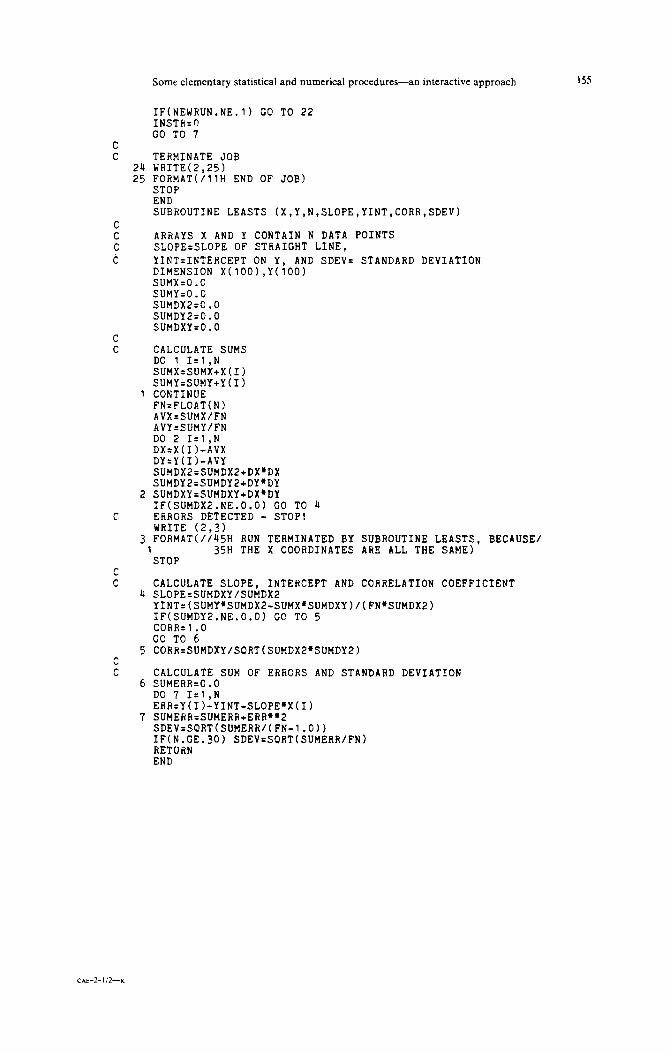
C C CALL SUBROUTINE TO FIT THE POLYNOMIAL

CALL POLY~NTERMS,X,Y,WEICHT,YC,RES,MAXORl,NORDER,GOODN,COEFF,L~ MAXOR=MAXORl-1 IF(L.EO.0) GO TO 23 WRITE(2.22) NORDER

24 FORMAT(141H MAXIMUM ORDER OF POLYNOMIAL TESTED FGR =,I3 1 /33H ORDER OF BEST POLYNOMIAL FOUND =,I31

C C

:;:

23 :

PRINT GOOCNESS OF FIT FOR THE VARIOUS CfiDERS WRITE(2.26) FORMAT(i36H POLYNOMIAL ORDER GOODNESS OF FIT) DO 28 I=l,MAXORl JDL=I-1 WRITE(2,27) JDL,GOODN(I) FORMAT(/~H ,7x,r2,13x,lPEl0.3) CONTINUE

PRINT COEFFICIENTS FOUND FOR THE BEST (OR SPECIFIED) POLYNOMIAL WRITE(2,29)

22 FORMAT(j32H ORDER OF POLYNOMIAL SPECIFIED =,I31 GO TO 25

23 WRITE(2,24) MAXOR,NORDER

29 FORMAT,;,;; FYEFFICIENTS OF THE BEST POLYNOMIAL 1 NORDl.NO;DER+l

= A + B4X + C'X"'2 + D"X**3 +...)/I

DO 31 I=l,NORDl WRITE(2,30) ICOEFF(I),COEFF(I)

30 FORMAT(lH ,AZ,lPE11.4) 31 CONTINUE

C C DECIDE WHETHER TO PRINT A TABLE OF RESICUALS

32 WRITE(2,33) 33 FORMAT(/50H TYPE 1 FOR A TABLE OF RESIDUALS, OTHERWISE TYPE 0

1 /19H THEN PRESS RETURN./) READ(1,3) ITABLE IF(ITABLE.EO.0) GO TO 39 IF(ITABLE.EO.1) GO TO 34 WRITE(2,4) GO TO 72

41 1 /19H THEN PRESS RETURN./) READ(1,3) NEWRUN IF(NEWRUN.EC.0) GO TO 44 INSTRnO IF(NEWRUN.EO.l) GO TO 7 WRITE(2,4) GO TO 41

C C

42 43

ENTER IF THERE ARE NOT ENOUGH POINTS WRITE(2,43) FORMAT(/4OH RUN TERMINATED - NOT ENOUGH DATA POINTS) GO TO 39

C C

44

45

TERMINATE JOB IF(INSTR.EO.0) GO TO 46 WRITE(2,45) FORMAT (50H REMEMBER THAT YOU MUST NOT EXTRAPOLATE BEYOND THE 1 /49H DATA POINTS, AND ALSO THAT INTERPOLATION BETWEEN 2 /49H POINTS IS DANGEROUS WITH HIGH ORDER POLYNOMIALS.)

WRITE(2,35) FORMAT(/49H X Y Y(CALC) DIFF/) RESID2rO.O DO 37 I=l,NTERMS WRITE(2.36) X(I).Y(I).YC(I).RES(I) FORMAT(iH ,4(1PEi2.4,iX)) RESID2=RESID2+RES(I)'*2 CONTINUE WRITE(2,38) RESID2 FORMAT(/24H SUM OF ERRORS SQUARED =,lPE11.4)

DECIDE WHETHER TO FINISH OR HAVE ANOTHER RUN WRITE(2,40) FORMAT(/40H TYPE 0 TO FINISH, OR 1 FOR ANOTHER RUN,

46 WRITE(2,47) 47 FoRMAT(3OH GOODBYE POLY I MUST LEAVE YOU//llH END OF JOB)

STOP- END SUBROUTINE POLY(NTERMS,X,Y,WEIGHT,YC,RES,MAXORl,NCRDER,GOODN, 1 C0EFF.L)


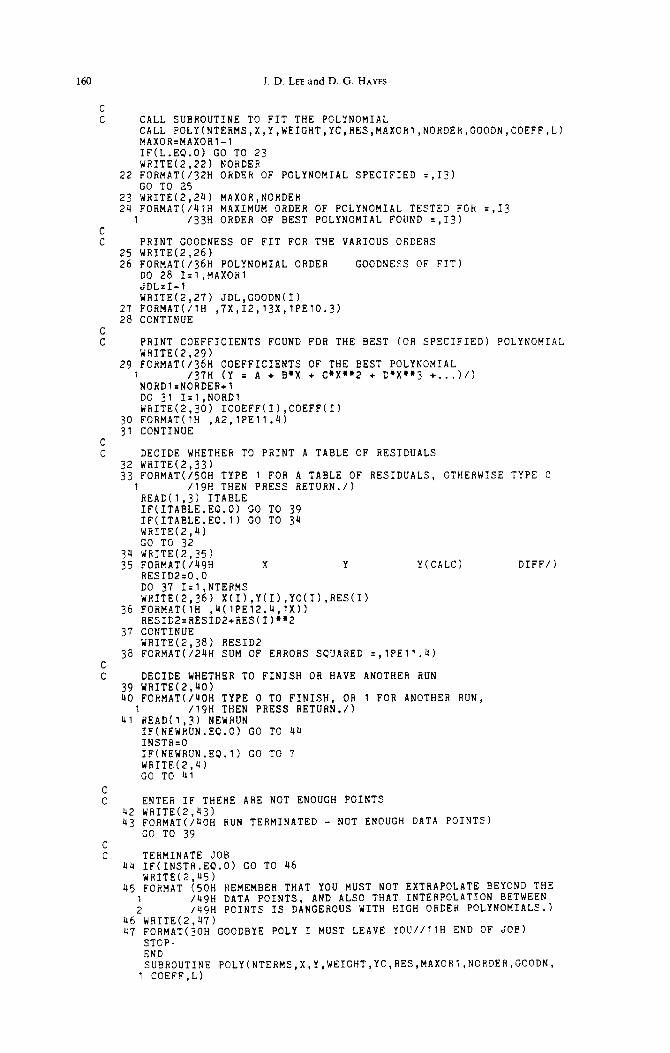
C C C C C C C C C C C C C C

: C

: C C G C

C

C C

SUBROUTINE TO CALCULATE A WEIGHTED LEAST SQUARES POLYNOMIAL BY FORSYTHE'S METHOD USING ORTHOGONAL POLYNOMIALS. NTERMS IS THE NUMBER OF DATA POINTS (MAX VALUE = 100) X t Y ARE ARHAYS CONTAINING THE DATA POINTS WEIGHT IS AN ARRAY CONTAINING THE WEIGHTS YC ARRAY CONTAINS THE CALCULATED Y COORDINATES ON ORIGINAL SCALE RES ARRAY CONTAINS (OBSERVED y - CALCULATED Y) ON ORIGINAL SCALE MAXORl IS THE MAXIMUM DEGREE OF THE POLYNOMIAL TO BE TESTED FOR +l NORDER IS SET ON EXIT TO THE DEGREE OF THE POLYNOMIAL FOUND GOODN IS AN ARRAY WHICH ON EXIT CONTAINS GOODNESS OF FIT TERMS

IE (SCALED SIGMA Y SOUARED/(NO.TERMS-ORDER-111 COEFF IS AN ARRAY WHICH ON EXIT CONTAINS THE COEFFICIENTS OF THE BEST POLYNOMIAL FOUND. IF ON ENTRY L=O THEN ALL THE POLYNOMIALS FROM 0 TO HAXORl-1 ARE EXAMINED, AND FROM THE GOODNESS OF FIT THE BEST POLYNOMIAL IS FOUND, AND THE CONSTANTS FOR THIS ARE REPORTED. IF ON ENTRY L-1 THEN THE POLYNOMIAL REPORTED IS OF DEGREE MAXORl-1. BOTH THE X k Y COORDINATES ARE SCALED IN THE SUBROUTINE TO REDUCE ROUNDING ERRORS. AX k BX ARE USED TO SCALE X TERMS, AY k BY TO SCALE Y TERMS.

DIMENSION X(lOO),Y(lOO),WEIGHT(lOO),DP(lOO),XP(100~ DIMENSION XS(lOO),YS(lOO),YC(lOO~,RES(100) DIMENSION GOODN(lO),COEFF(lO),AL(lO),BA(lO),S(10) DIMENSION CA(lO),CE(lO),CC(10),CD(ll)

HAXORD-MAXORl-1 NORDER=MAXORD DO 1 I=l,MAXORl CC(I)=O.O BA(l)=O.O CD(l)=O.O CD(2)=0.0 CAil)=l.O DELSO=O.O PM-O.0 SUMW=O.O GOOMIN-0.0 IFLAG=O SIGW=WEIGHT(l)

FIND THE MAXIMUM XMAX=X(l) XMIN=X(l) YMAX=Y(l) YMIN.Y(l) DO 2 I=Z,NTERMS IF(X(I).GT.XMAX) IF(X(I).LT.XMIN) IF(Y(I).GT.YMAX) IF(Y(I).LT.YMIN)

AND MINIMUM X k Y

XMAX=X(I) XMIN=X(I) YHAX=Y(I) YMTN=Y(I)

IF(WEIGHT(I).LT.O.O) GO TO 23 SIGW=SIGW+WEICHT(I) IF(SIGW.EO.O.0) GOT0 21 AY=(YMAX+YMIN)/Z.O BY=(YMAX-YMIN)/Z.O IF(BY.GT.O.0) GO TO 3 COEFF(l)=Y(l) NOHDER-0 RETURN

SCALE Y TERMS DO 4 I=l,NTERMS YS(I)=(Y(I)-AY)/BY DELSC=DELSO+WEIGHT(I)"YS(I)**2 DP(I)=l.O XP(I)=O.O PM.PM+WEIGHT(I)*Y.S(I) SUMWsSUMW+WEIGHT(I) S(l)sPM/SUMW CC(l)=S(l) DELSQ=DELSO-S(l)*PM GOODN(l)=ABS(DELSO/FLOAT(NTERMS-1)) AX=i.O/(XMAX-XMIN) BX.-2.0-AX'XMIN

162 J. D. L~~and D.G. HAYES

C C SCALE X

DO 5 ;=l,NTERMS = "S(I)=AX*X(I)+BX

c - C START LOOP FOR EACH ORDER

DO 13 I=l,HAXORD DUzO.0 DO 6 J=l,NTERHS

6 DIJ=DU+WEICHT(J)'XS(J)'DP(J)*"2 AL(I+l)=DU/SUMW XW=SUMW SUMW=O.O PM=O.O DO 7 J=l,NTEAMS DU=BA(I)*XP(J) XP(J)=DP(J) DPijj=(XS~j)-AL(I+l))tDP(J)-DU SUHW=SUHW+WEIGHT(J)'DP(J!**2

7 PM=PM+WEICHT(J)'YS(J)*DP(J) BA(I+l)=SUMW/XW S(I+l)=PH/SUMW DELSQ-DELSQ-S(I+l)*PM COODN(I+l)=ABS(DELSQ/FLOAT(NTERMS-I-1)) IF(L.CT.0) GO TO 10

C C ENTER IF PROGRAM HAS TO DECIDE ON BEST ORDER (LEO)

IF(IFLAC.EQ.l) GO TO 9 IF(COODN(I+1).LT.COODN(I)) GO TO 10

C ENTER IF A MINIMUM DETECTED NGRDER=I-1 IFLAC=l COOMIN=GOODN(I) DO 8 J=l,MAXbRl

8 CB(J)=CC(J) GO TO 10

9 IF (COODN(I+l).GE.(O.6~GOOMIN)) GO TO 13 IFLAG- NORDER-MAXORD

C 10 DC 11 J-1,1

DU=CD(J+l)*BA(I) CD(J+l):CA(J) CA(J)=CD(J)-AL(I+l)'CA(J)-DU

11 CC(J)=CC(J)+S(I+l)*CA(J) CC( I+l)=S(I+l) CA(I+l)=l.O CD(I+2)=0.0 IF(IFLAG.EQ.0) GO TO 13 IF(I.NE.MAXORD) GO TO 13 DO 12 J=l,MAXORl

12 CC(J)=CB(J) 13 CONTINUE

CD(1)sl.O CB(l)=l.O COEFF(l)=CC(l) DO 14 I=P.MAXORl CD(I)=l.O. CB(I)=BX*CB(I-1)

14 COEFF(l)=COEFF(l!+CC(I)*CB(I) DO 16 Jz2,MAXORl CD(l)=CD(l)*AX COEFF(J)+CC(J)*CD(l) KK=2 Jl=J+l IF(Jl.GT.MAXORl) GO TO 17 DO 15 I=Jl,MAXORl CD(KK)=AX*CD(KK)+CD(KK-1) COEFF(J)=COEFF(J)+CC(I)*CD(KK)*CB(KK)

15 KK=KK+l 16 CONTINUE

C C CALCULATE YCALC h RESIDUAL FOR EACH PCINT (ON ORIGINAL SCALE).

17 DO 19 I=l,NTERMS J=NORDEH+l YCAL=COEFF(J) DO 18 K=l,NORDER YCAL=COEFF(J-l)+(X(I)*YCAL)

Some eiementary statistical and numerical procedures-an interactive approach 163

18

19 C C

20

C

H:

23 24

JrJ-1 YC(I)=YCAL"BY+AY RES(I)=(YS(I)-YCAL)*EY

CONVERT COEFF ARRAY BACK TO ORIGINAL SCALE COEFF(lf=tCOEFF(l)*BY)+AY DO 20 I=Z,MAXORl COEFF~I)=COEFF(I)*BY CONTINUE RETURN ENTER IF ERRORS DETECTED WRITE(2,22) FORHAT(51H JOB TERMINATED BY PROGRAM BECAUSE SUM OF WEIGHTS=01 STOP WRITEf2,24) FORMAT(46H NEGATIVE WEIGHTS NOT PERMITTED-NUN TERMXNATED) STOP END

Trial run with POLYNOMIAL program

PROGRAM TO FIT A POLYNOMIAL THROUGH A SET OF POINTS e====== == rt: : f========= =::z=== = =t+ 55: x=5===

TYPE 1 FOR FULL INSTRUCTIONS, OTHEffWISE TYPE 0 THEN PRESS RETURN ?l

TYPE IN X L Y VALUES SEPARATED BY A SPACE. THEN PRESS RETURN, AND TYPE THE NEXT PAIR OF VALUES TERMINATE DATA WITH BOTH X AND Y EQUAL TO 999999.

STARTING DATA X Y

? -1. ? 0. :* ? 1. 1: ? 2. ? 2.5 43175 ? 999999. 999999.

TYPE 0 IF ALL THE POLYNOMIALS FROM ORDER O-9 ARE TO BE EXAMINED, AND THE ONE WHICH FITS BEST REPORTED, OR TYPE IN THE ORDER REPUIRED IN THE RANGE l-9 OF THE ONE SPECIFIC POLYNOMIAL REQUIRED. THEN PRESS RETURN. ?O THE MAXIMUM ORDER HAS BEEN REDUCED BECAUSE OF THE LIMITED NUMBER OF DATA POINTS PROVIDED,

MAXIMUM ORDER OF POLYNOMIAL TESTED FOR o 3 ORDER OF BEST POLYNOMIAL FOUND = 2

POLYNOMIAL ORDER GOODNESS OF FIT 0 7.1473-01

1 ?.290E-01

2 O.OOOE 00

3 2.032E-21

COEFFICIENTS OF THE BEST POLYNOMIAL (Y = A + B'X + C*X'*2 + D*X**3 +...I

A= l.OOOOE 00 B=-l.OOOOE 00 C- l.OOOOE 00

TYPE 1 FOR A TABLE OF RESIDUALS, OTHERWISE TYPE 0 THEN PRESS RETURN. ? 0

TYPE 0 TO FINISH, OR 1 FOR ANOTHER RUN, THEN PRESS RETURN. ?O

GOODBYE POLY 3: MUST LEAVE YOU

END OF JOB

164 _I. D. LEE and D. G. HAYES

kind: supposing we havea process which generates random rtumbers, such that each number generated is one of a known finite set of numbers. Suppose we generate a sequence of random numbers and observe the frequency with which each possible value occurs. Suppose we adopt the hypothesis that all possible values are equally likely. If the observed frequencies are not all equal, what is the proba- brlity that a discrepancy such as the observed discrepancy could have arisen by chance?

One important applic?tion of the chisquared test is as follows: suppose we have a process for generating random numbers, and we are testing the hypothesis that the process generates numbers according to some given theoretical probability distribution function, such as the normal distribution. Suppose we have a sample of numbers generated by the process. We can proceed as follows. Consider the range within which the numbers can lie, according to the theoretical distribution. Divide the range into a suitable number of intervals, such that a random number with the theoretical distribution is equally likely to he in any of the intervals. Note how many numbers of the given sample lie in each interval, and apply the chi-squared test to the frequencies so obtained.

The theoretical distribution may have parameters; for example, in the case of the normaf distribution the parameters are the mean and the variance. The program we are considering assumes that the parameters are not deduced from the sample of random numbers we are using. For example, in the case of the normal distribution, it is assumed that the mean and variance are not deliberately made equal to the mean and variance of the sample.

In the discussion so far, it has been assumed that the theoretical frequencies are ail equal. The chi- squared test can be used to deal with the case where the theoretical frequencies are unequal. However. the program we are concerned with assumes that the theoretical frequencies are equal.

The program takes as input the theoretical frequency, and the observed frequencies. The theoretical frequency is assumed to be the mean of the observed frequencies; the program will not give correct results if it is not. The program outputs the value of x2. the number of degrees-of-freedom, and the appropriate probability.

The value of x2 is given by:

1 x2 = ;x(i;; - t)”

where t is the theoretical frequency and the vi are the observed frequencies. The number ofdegrees-of-

freedom is one less than the number of observed frequencies. The probability calculated by the program is the probability of a value of x2 at least as great as the observed value arising by chance, on the assumption that the theoretical model applies. Thus, a very small probability suggests that the theoretical model is probably not correct. A probability very close to 1007: might also cause one to suspect the theoretical model.

The quantity x2 has probabiliry density function:

where v is the number of degrees-of-freedom. Hence the probability calculated by the program is given by:

xvI2 - 1 e-“‘d.u.

If the substitution z = xi2 is made in f I), this gives:

P 1 _=- J

c ,“~3-1 +2 -

e-‘dz. 100 T(vi2)

A description will now be given of how (2) is evaluated. It can be shown that:

J x0 e-” dx = --.y“ e-* f aj.f- 1 e-I dx_,

The gamma function satisfies the following two equations:

l-(n) = I .2.3.. . (n - 1)if n isapositive integer

T(n f +) = Jn _ $. $. . In - 2) if n is a non-negative integer

(1)

12)

13)

(4)

15)


From (4) and by repeatedly using (3), it can be shown that, if n is a non-negative integer:

s x”e-“dx= -I(n+ l)emX l+x+c+-++.. X3 X”

+-----. I-(3) U4) T(n + 1) >

From (5), and by repeatedly using (3), it can be shown that, if n is an integer which is non-negative or equals - 1. then :

Suppose we define a function Q, by:

0((x) =d& X _ ~ e-“” dt.

It can be shown that (o( so) = 1.

It can also be shown that:

Jx-f eeX dx = 2Jrr@[J(2.x)].

From (7) and (10) it can be seen that:

(7)

(8)

(9)

(10)

” X2

J( !+ r+ 111+ . ..+ l,z Xn n i i.; .

(11) 2’2’2 2 2....(n + 4, >I

From (2) (4) and (6) it can be shown that:

P .2 .v/2- 1 ’ 4

100=e 1+Y+L+...+ 2 2.4 2.4...(v - 2)

where Y = x2, if v is even. (12)

From (2) (9) and (I 1) it can be shown that

P - = 2 = 2@(JY) + e-y/2

2Y

J! - 1 + i + & + . + y

(V-3)/2

100 n 3.5....(v - 2) >

where Y = x2, ifv is odd. (13)

One problem is how to evaluate the function Cp. The program uses the following method. A polynomial p can be found such that l/p(~)~ IS an approximation to 2 - 2@(x) whenever x is positive.

The program uses this polynomial to evaluate the right-hand side of (13). If x is large, then ~/P(x)~ is not a good approximation to 2 - 2@(x), if the error is measured as a fraction of the quantity being approximated. However, when x is large, both ~/P(x)~ and 2 - 2@(x) are close to zero, and so the error is not serious. If v is large, then care must be taken when evaluating (12) and (13), otherwise floating point overflow may occur.

Introduction F AND I TESTS

These two statistical tests are widely used to compare two groups of experimental measurements. The t test is used to determine whether the mean of one group differs significantly from the mean of the other group. More precisely, the t test calculates the probability that the observed difference in means could have arisen by chance on the assumption that the numbers were chosen at random from the same population of normally distributed random numbers. Hence a large probability suggests that the difference is not significant, and a small probability suggests that it is.

The F test determines whether the variance of one group differs significantly from the variance of the other. More precisely, the F test calculates the probability that the observed difference in variance could have arisen by chance, on the assumption that the numbers were chosen at random from the same population of normally distributed random numbers.

The t test assumes that the two groups of measurements have the same variance. If there is a big difference in variances, then the t test should not be regarded as reliable. The difference in variances may have arisen by chance, and the F test can be used to estimate how likely this is.

166 J.D.LEE~~~ D.G. HAYET

Listing of CHI-SQUARE program

WRITE (2,l) 1 FORMAT (//17H CHI-SC'UARED TEST

2 FORMAT (19H THEN PRESS RETURN.) 3 READ (1.4) INSTR 4 FORMAT (ill

C IF POSSIBLE THE ABOVE FORMAT SHOULD BE REPLACED BY c 4 FORMAT (IO)

IF (INSTR.E~.~.OR.INSTR.EP.~) GO TO 6 WRITE (2,5) FORMAT (/35H INCORRECT NUMBER TYPED - TRY AGAIN) GO TO 3 WRITE (2,7) FORMAT (/31H TYPE THE THEORETICAL FREQUENCY) IF (INSTR.EQ.~) WRITE (2,2) READ (1.9) T FORMAT (F7.0)

FREE FORMAT

5

6 7

0 9

C c 9

IF POSSIBLE THE ABOVE FORMAT SHOULD BE REPLACED BY FORMAT (FO.0)

FREE FORMAT

IF (T.GT.O.0) GO TO 14 IF (T.LT.O.0) GO TO 11 WRITE (2,lO)

10 FORMAT(/54H PROGRAM WILL NOT WORK WITH THEORETICAL GO TO 11

FREOUENCY OF 0)

11 12 1?

WRITE (2,121 FORMAT (136~ NEGATIVE FREOUENCIES ARE IMF~SSIBLE)

14 15

WRITE (2,5) GO TO 8 WRITE (2.15)

16

FORMAT (;52H TYPE IN THE OBSERVED DATA IF (IN~TR.EQ.~) WR:TE (2,161

FREGUENCIES ONE AT A TIME)

FORMAT (30H PRESS RETURN AFTER EACH TERM. 1 /39H TERMINATE DATA WITH A VALUE OF 999999.)

C INPUT DATA VALUES NTERMS=O s=o.o DO 17 1=1,500 READ (1.9) V

1 /17H === ______- ==== _______ 2 /14H WOULD YOU LIKE FULL INSTRUCTIONS? 3 /28H TYPE 1 FOR YES OR 0 FOR NO.) WRITE (2,2)

IF (V.Eb.999999.) GO TO 19 S=S+(V-T)**2 NTERMS=NTERMS+l

17 CONTINUE WRITE (2.18)

18 FORMAT (/35H PROGRAM CAN ONLY HANDLE 500 VALUES) C C ABANDON RUN IF LESS THAN 2 TERMS

19 IF (NTERMS.GE.2) GO TO 21 WRITE (2,201

20 FORMAT (/42H ATTEMPT TO RUN WITH THIS DATA ABANDONED - 1 /36H BECAUSE THERE ARE NOT ENOUGH TERMS.) GO TO 29

21 CHISQ=S/T NDEGFR-NTERMS-1 WRITE (2,221 CHISQ,NDEGFR

22 FORMAT (/23H VALUE OF CHI-SOUARED =,F10.5 1 /21H DEGREES OF FREEDOM =,I3) IF (CHISQ.EO.O.0) WRITE (2.23)

23 FORMAT (/69H THE OBSERVED VALUES ALL AGREE EXACTLY WITH THE THEORE 1TICAL FREGUENCY) E2=EXP(-10.0) GZ=CHISQ/2.0 Sl-0.0 Wnl.0 Jr2 Ml=NDEGFR+l IE-0 IF (NDEGFR.EO.2*(NDEGFR/2)) GO TO 25 IE-1 J=3 GO TO 25

24 Sl=Sl+W W=W*CHISC!/FLOAT(J) J=J+2 IF (W.LT.lOOOOO.0) GO TO 25 ;l;S;;E2

G;eG2-lo.o 25 IF (J.LT.Ml) GO TO 24

P2=EXP(-C2)*Sl P-P2 IF (IE.EO.0) GO TO 26 Z=SORT(CHISO)

26

P1=~~~~.0057l1*z-.006523~*z+.038704)*z+.094513)*z+.200039)*Z~l.0 P=l.O/P1**4+SORT(2.0*CHISO/3.l4l59)*P2 P.loo.o*P WRITE (2,271 P

27 FORMAT (/47H PROBABILITY THAT EXPERIMENTAL DATA AGREES WITH 1 /33H THEORETICAL VALUE IS WITHIN THE , 2 F5.l,14H PERCENT LIMIT)

C c DECIDE WHETHER TO TERMINATE JOB OR HAVE ANOTHER RUN WRITE (2,28)


28 FORMAT (/39H TYPE 0 TO FINISH OR 1 FOR ANOTHER RUN.) IF (INSTR.EO.~) WRITE (2,2)

29 READ (1,4) NEWRUN IF (NEwRuN.E~.O) Go TO 31 IF (NEwRUN.EO.~) Go TO 30 WRITE (2,5) GO TO 29

30 INSTR=O GO TO 6

C C TERMINATE JOB

31 WRITE (2,321 32 FORMAT (/54H THERE ARE LIES, DAMNED LIES AND STATISTICS...DISRAELI

1 //28H JOB COMPLETED SUCCESSFULLY.) STOP END


Trial run with CHI-SQUARED program

CHI-SQUARED TEST === ===z==z s=== WOULD YOU LIKE FULL INSTRUCTIONS? TYPE 1 FOR YES OR 0 FOR NO. THEN PRESS RETURN. ?1

TYPE THE THEORETICAL FREQUENCY THEN PRESS RETURN. ? b5.

TYPE IN THE OBSERVED DATA FREQUENCIES ONE AT A TIME PRESS RETURN AFTER EACH TERM. TERMINATE DATA WITH A VALUE OF 999999. ? 41. ? 49. ? 45. ? 45. ? 45. ? 999999.

VALUE OF CHI-SQUARED I 0.71111 DEGREES OF FREEDOM = 4

PROBABILITY THAT EXPERIMENTAL DATA AGREES WITH THEORETICAL VALUE IS WITHIN THE 95.0 PERCENT LIMIT

TYPE 0 TO FINISH OR 1 FOR ANOTHER RUN. THEN PRESS RETURN. ? 0

THERE ARE LIES, DAMNED LIES AND STATISTICS...DISRAELI



interpretation of results

The provability calculated by the t test can lie anywhere between 0 and 100 %. If the means of the two groups are equal, then the probability will be 100 %. If the means diJJer greatly, then the probability will be near 0 %. The probability calculated by the F test will never be more than 50 %, Indeed, if a probability of more than 50 % is obtained, then this probabiiity P is replaced by 100 % - P. This operation is equivalent to interchanging the two groups of numbers. If the two groups ofnumbers are identical, then the F test probability will be 50 %.

Cu~c~~ation of variance

One problem in the F and t tests is how to calculate the variance. If the given readings in one group are :

x1, X2’ x3,. . . x I)

then the variance is defined as

;. -y(Xj - ny

where n is the number of readings, and Z the mean of the readings. The variance may be calculated by first evaluating the mean, and then the differences between each reading and the mean. This has the disadvantage that all the numbers must be stored, thus making the program very big.

An alternative method would be to use the fact that:

This has the disadvantage that it may involve subtraction of two large and nearly equal quantities, leading to Iarge rounding off errors.

The method used is as follows-let (~1~ denote the average of x1, x2, . . . xj. Then it can be shown that

Equation (1) can be used to calculate the variance, avoiding the necessity for storing a large number of data values. The rounding off errors produced are much smaller than those from the second method of calculating the variance, and are not signi~cantly different from those in the first method.

Tests performed by the program

The data values input by the user are tested to ensure that they are suitable for the tests involved. If the vaiues are unsuitable for the t test, they will also be unsuitable for the F test. However, the values might be suitable for the r test but not for the F test. The criteria used to determine suitability are given beiow. The following are needed for both the F test and the I tests:

(a) There must be at least one data value in each group. (b) There must be at least three values in the two groups combined. (c) The numbers in the two groups combined must not all be the same.

The following are needed for the F test but not for the r test:

(a) Each group must have at least two numbers in it. (b) Neither group can have more than sixty numbers in it. (This restriction is imposed because of

floating point underflow and overflow whrch occurred at lo-t8 and 10” respectively on the test computer. If the program is run on a different computer this limit may be changed.)

fcf It is not permissible to have the numbers in one group all equal, and the numbers in the second group all equal but different from the numbers in the first group.

~alc~l~t~on of the t test pro~~bil~t~

if the numbers in one group are equal, and the numbers in the other group are equal, and the numbers in one group are not the same as the numbers in the other group, then the t test probability is 0 %. Otherwise the quantity r is calculated:

170 J. D. LEE and D. G. HAYS

where P,, _?a are the means of the two groups of numbers, nA, n,, are the numbers of readings in the

two groups, and So, sa are the standard deviations. The standard deviation used in (2) is defined as the square root of the variance and differs from that reported by the program (see later). The t test probability is then calculated by

P 2 1-(jv + i)

I

= dt -=_--_ loo j(bk) l-(fv) ,*P, (1 + t2/vp+ ”

(3)

where tp is the value of r calculated from (2) and y = (total number of readings) - 2. An outline of how (3) is eva!uated is given below: If the substitution t = v/y tan 19 is made. one obtains

s n/2

~- =

v!v cos”- ’ I.3 d0.

la” - ’ il& 1 ” (4)

n-l It can be shown that cos” Ode = ! sin 0 COS”- ’ 8 + - COST- 2 e de. (5)

n n

By repeatedly using (5), it can be shown that

r c09ede = !sinecOs~-le + n-l - sin tI cosn- ’ e +

d n n(n - 2)

(n f

- 1). . .5.3 sin e cos e + (n - 1). 3.1

n(n - 2). .4.2 tI

n(n - 2). . .4.2 if n is even and (6)

I COST e de = ! sin e COS”- 1 e + n-l

___ sin e COS”- ’ e -c n n(n - 2)

+ (n - 1). . ‘6.4 sin e cos2 e f (n - 1) . .4.2 sin e

n(n - 2). . 5.3

if n is odd,

n(n - 2). 5.3

If n is an integer, T(n) = (n - l)(n - 2). .2.1

T(n + i) = (n - +)(n

From (3) (4) (6) (7) (8) and (9) it can be deduced

- 2) .3_ . &/7x

(7)

(8)

(9)

1 where u = ~

1 f qv if Y is even and

P 2 - = 1 - ;

Irpl 2.4. (v - 3) uP-3)/2

100 { tan- l T + J[u(l - u)]

4v i 1 + : u + g 2 + . +

3.5. (v - 2) >I

1 where u = ~

1 + tpv if v is odd. ill)

Note that in equation (11) no terms of the series are taken if v = 1.

Calculation of F test probability

To calculate the F test probability, it is first necessary to calculate the quantity F, defined by

F= EA(%l - 1,s: (12)

‘&A - 1)s;

where n,, nB are the numbers of numbers in the two groups, and S,, sR are the standard deviations. The F test probability is then calculated from

P r+, + ~v*)vi”* tY2 = F+' -I

-= 100 r(+v,)r(:v,) 1 ‘2 F,(~2 + v~F)*‘“~+“~)

dF (13)

where FP is the value of F calculated by (12), and vr = (number of numbers in first group) - 1, and v2 = (number of numbers in second group) - 1. If the substitution F = (v2ivI) tan ‘0 is made, it can


be shown that

s

Q FfVl- I 2

I

n/Z dF = - sin”- ’ 0 COP- * 0 de.

p, (v2 + v~F)+(~~+“~) Vyv$” tan-’ JlFv,/rd

It can be shown that

I

1 n-l sin” O cosm tId6 = - -sin”-l ecosm+le + - sin”- 2 e COP e dtI.

m+n m+n

By repeatedly using (15) it can be shown that

1 n-1 sin” 0 cosm 0 d6 = - -sin”-’ ecosm+l e - sinnV3 e coP+l 0

m+n (m + n)(m + n - 2)

It can be shown that

(n - 1)...4.2 COP’+ ’ 0 if n is odd.

(m + n) . (m + 3)(m + 1)

5 1 m-l sin” 6 COP e de = -sin”+ l e COP-* e + -

s sin” e cosm- 2 e de.

nfm n+m


I

1 -sin”+’ ecOsm-le+

m-l sin” e CO? e de = sin”+ 1e~~~m-3 e +

n+ m (n + m)(n + m - 2)

+ (m - 1)...4.2

sin”+ ’ 0 if m is odd. (n + m). . (n + 3)(n + 1)


s

1 n-l sin” 8 ~0s'" e de = - -sin”-*ecOs~+le - siC3 O cos*+1 e

m-k n (m + n)(m + n - 2) -

(14)

(15)

(16)

(17)

(18)

. . .

(n - 1). . .5.3 sinfIcos”+‘e+

(n - 1)...3.1

(m + n). (m + 4)(m + 2) (m-t n)...(m+ 4)(m+ 2) I co? e de if n is even. (19)

From (6) and (19) it can be shown that

1 n-l sin” e cosm e de = - -sin”-’ ecosm+l e - sinnm3 eCOSm+le - . .

m+n (m + n)(m + n - 2)

(n - I)...53 sintIcos”+‘e +

(n - 1)...3.1

- (m + n). (m + 4)(m + 2) sine COS"-l e

(m + n). . . (m + 2)m

+ (n - 1)...3.l.(m - l)sinecos~_3e+ ., + (n - 1)...3.l.(m- l)5.3sinecose

(m + n). . . m(m - 2) (m + n), . .4.2

+ (n - 1). ..3.1 (m - I)... 3.1 6 if m and n are even.

(m + n). .4.2

From (8) (9) (1.1) and (16), it can be shown that

& = (1 - 442 l+$U+ v*(vz + 2) (v* + 2). . . (v2 + VI - 4) uy,,2_l

2.4 112 + . . + v*

2.4.. . (vl - 2) > 1

whereu = 1 + (lIF&JvJ

if \I, is even.

From (8), (9) (13) and (18) it can be shown that

P - = 1 - (1 - up2 vl(\l’ + 2)

u2 + . . . + Vl(VI + 2). . . (VI + v2 - 4) aY2:2 - 1

100 2,4

2.4.. . (v2 - 2) >

(20)

(21)

1 where u =

1 + F,b,lv,) if v2 is even.

c*E-2-1/2-L

(22)

172 J.D.LEE~~~ D.G. HAYES

Listing of F AIVD t TESTprogram

DIMENSION K(2),A(2),Y(2) WRITE (2,l) FOfiMAT (//15H F AND T TESTS./lSH 5 === = =====I) WRITE (2,2) FORMAT (/47H TYPE 1 FOR FULL INSTRUCTIONS, OTHERWISE TYPE 0

/19H THEN PRESS RETURN.) EALL REPLY (INSTR) DO a Jr1,2 A(J)=O.O Y(J)=O.G AIrl.0 Z=O.O WRITE (2,4) J

4 FORMAT (/2aH INPUT THE NUMBERS IN GROUP ,111 IF (1~sTR.Ec.l) WRITE (2,5)

5 FORMAT (/32H PRESS RETURN AFTER EACH NUMBER.

a

9

10 11

12

13 14 15

16 17

la

19

20

21

22

1 /32H AND TERMINATE DATA WITH 999999:) READ (1,7) X FORMAT (F10.5) REPLACE THE ABOVE FORMAT BY FREE FORMAT IF AVAILABLE FORMAT (FO.0) ;FZL;.EQ.999999.) GO TO a

X:=X-Y(J) A(J)=A(J)+Xl*Xl*(AI-l.O)/AI Y(J)=Z/AI AI=AI+l.O GO TO 6 K(J) IS THE NUMBER OF POINTS IN THE CURRENT GROUP K(J)=IFIX(AI)-1 DO 17 Jr1,2 IF (K(J).GT.o) GO TO lo WRITE (2,9) J FORMAT (/6H GROUP,I2) GO TO 14 WRITE (2,111 J,Y(J) FORMAT (/6H GROUP,IZ,aH MEAN =,lPE10.3) WRITE (2.12) A(J) FORMAT (;26H SUM OF ERRORS SOUARED =,lPE10.3) IF (K(J).EQ.~) GO TO 14 SD=SORT(A(J)/FLOAT(K(J)-1)) WRITE (2,13) SD FORMAT (/23H STANDARD DEVIATION .,lPE10.3) WfiITE (2.15) K(J) FORMAT (j26H NUMBER OF DATA POINTS ~~13) Kl=K(J)-1 WRITE (2,16) Kl FORMAT (1338 NUMBER OF DEGREES OF FREEDOM =,I!) CONTINUE IVl=K(l)-1 IF :IVl.LT.O) WRITE (2,181 FORMAT (/31H TOO FEW NUMBERS IN FIRST GROUP) IV2=K(2)-1 IF (IV2.GE.0) GO TO 20 WRITE (2.19) FORMAT (j32H TOO FEW NUMBERS IN SECOND GROUP) GO TO 69 IF (IVl.LT.0) GO TO 69 1v=1v1+1v2 IF (IV.GT.0) GO TO 22 WRITE (2,21) FORMAT (/4OH TOO FEW GO TO 69 04=A(l)+A(21 IF (ti4;GT;O;O) GO TO 24 IF (Y(l).NE.Y(E)) GO TO 24 WRITE (2.23)

23 FORMAT (/35H F AND T 1 /3aH BECAUSE

NUMBERS IN BOTH GROUPS COMBINED)

TEST RESULTS INDETERMINATE, ALL THE DATA VALUES ARE EOUAL)

GO TO 69 THE FOLLOWING LINES PERFORM THE T TEST

24 WRITE (2.25) 25 FORMAT (j36H WOULD YOU LIKE TO PERFORM A T TEST?)

IF (INSTR.NE.O) WRITE (2,26) 26 FORMAT (/31H TYPE 1 IF SO, OTHERWISE TYPE 0)

CALL REPLY (ITT) IF (ITT.EQ.0) GO TO 39


27

28

29

30

31

32

33

34

35

36

37 38

C

z:

41

42

43

44

45

46

47

48

49

50

51

52

53

IF (Q4.GT.0.0) GO TO 27 PzO.0 GO TO 37 S.SQRT(FL0AT~K~1~*K~2~*1V~/~FL0AT~K~1~+K~2~~*Q4~~ T=ABS(Y(l)-Y(2))*S WRITE (i,28) T FORMAT (/24H CALCULATED VALUE OF T =.lPE10.3) Kl=0 AJrl.0 IF (IV.EO.(IV/2)"2) GO TO 29 Kl=1 AJ=2.0 w-1.0 s-o.0 U=l.O/(l.O+T*T/FLOAT(IV)) GO To 31 s=s+w ;iW;;:;J;'AJ+l.O'

= IF (AJ.LT.FLOAT(IV)) co TO 30 IF (Kl.EO.1) GO TO 32 P=lOO.Or(l.O-SORT(l.O-U)*S) GO TO 33 Tl=ATAN(T/SQRT(FLOAT(IV))) P2=2.0/3.14159 P=lOO.O*(l.O-P2*(T1+SQRT(U'(1.0-U))'S)) IF (P.LT.5.) GO TO 35 WRITE (2,341 P FORMAT (/21H T TEST PROBABILITY =,F5.1) GO TO 39 IF (P.LT.0.5) GO TO 37 WRITE (2,36) P FORMAT (/21H T TEST PROBABILITY =,F6.2 Go TO 39 WRITE (2,38) P FORMAT (/21H T TEST PROBABILITY =,F7.3 1 THE FOLLOWING LINES PERFORM THE F TEST WRITE (2.40) FORMAT 037H WOULD YOU LIKE TO PERFORM IF (INSTR.NE.0) WRITE (2,261 CALL REPLY (IFT) IF (IFT.EQ.0) GO TO 69 IS9=0 IF (IVl.GT.0) GO TO 42

AN F TEST?)

WRITE (2,411 FORMAT (/42H TOO FEW NUMBERS IN FIRST GROUP FOR F TEST) IS9=1 IF-(IV2.GT.0) GO TO 44 WRITE (?,43) FORMAT (/43H TOO FEW NUMBERS IN SECOND GROUP FOR F TEST) IS9=1 IF (IVl.LE.60) GO TO 46 WRITE (2,451 FORMAT (/43H TOO MANY NUMBERS IN FIRST GROUP FOR F TEST) IS9=1 IF (IV2.LE.60) GO TO 48 WRITE (2.47) FORMAT (/44H TOO MANY NUMBERS IN SECOND GROUP FOR F TEST) IS9=1 IF (04.GT.O.O) GO TO 50 WRITE (2,491 FORMAT (/28H F TEST RESULT INDETERMINATE) GO TO 69 IF (IS9.EO.l) GO TO 69 IF (A(21.GT.O.O) GO Tb 51 PIO.0 GO TO 67 F=FL0AT(1V2)*A(1)/(FL0AT(1V1~*A(2)) WRITE (2,52) F FORMAT (/24H CALCULATED VALUE OF F .,lPE10.3) IE=O IF (IVl.EO.(IV1/2)*2) GO TO 5.3 IF (IV2.EQ.(IV2/2)*2) GO TO 54 GO T@ 58 U=l.O/(l.O+FLOAT(IV2)/(F'FLOAT(IV1))) Pl=FLOAT(IVl+l) Q=FLOAT(IVZ-2) GO TO 55

174 J. D. LEE and D. G. HAYIS

54 IE=l U=l.O/(i.O+F*FLOAT(IVl)/FLOAT(IV2)) Pl=FLOAT(IV2+1) O=FLOAT(IVl-2)

55 s=o.o W=l.O AJz2.0

56 SrS+W W=W*U'(AJ+Q)/AJ AJ=AJ+Z.O IF (AJ.LT.P~) GO TO 56 Z=SORT(l.O-U) IF (IE.EQ.~) co TO 57 P=100.0*(1.0-S*(Z**Ivl)) GO TO 63

57 P=100.0*S*(Z*fiIV2) GO TO 63

58 ;=;.'$.O+F*FLOAT(IVl)/FLOAT(IV2))

s:o:o wz1.0 AJz2.0 PlzFLOAT(IV2) GO TO 60

59 s=s+w W=W"IJ*AJ/(AJ+l.O)

60

61

62

63

64

65

66

:; 69 70

AJ=AJ+2.0 IF (AJ.LT.P~) ~0 TO 59 W=W*FLOAT(IV2) AJn3.0 Pl=FLOAT(IVl+l) Q=FLOAT(IV2-2) GO TO 62 s=s-w W=W'X'(AJ+O)/AJ AJ=AJ+2.0 -- IF (AJ.LT.~~) GO TO 61 T1=ATAN(SQRT(F‘FLOAT(IVl~/FLOAT(IV2))) Sl=S*sQRT(X'U) P-100.0*(1.0-2.0*(Tl+Sl)/3.14159) IF (~.~~.50.0) p=loo.o-p _ IF (P.LT.5.) GO TO 65 WRITE (2.64) P FORMAT (;21H F TEST PROBABILITY =,F5.1) GO TO 69 IF (P.LT.0.5) GO TO 67 WRITE (2,661 P ;C&R;;T6;/21H F TEST PROBABILITY =,F6.2)

WRITE (2.68) P FORMAT.(/ZlH F TEST PROBABILITY =,F7.3) WRITE (2.70) FORMAT (;/28H WOULD YOU LIKE ANOTHER RUN?) IF (INSTR.EO.~) WRITE (2,26) CALL REPLY (IAR) INSTR=O IF (IAR.EO.~) ~0 TO 3 WRITE (2.71)

71 ;,";'p'AT (/llH END OF JOB)

END C SUBROUTINE TO CHECK REPLIES

SUBROUTINE REPLY (J) 1 READ (1,2) J 2 FORMAT (11)

C REPLACE THE ABOVE FORMAT BY FREE FORMAT IF AVAILABLE C 2 FORMAT (IO)

IF (J.EP.O.OR.J.EQ.1) GO TO 4 WRITE (2,3)

3 FORMAT (/33H INVALID NUMBER TYPED. TRY AGAIN.) GO TO 1

4 RETURN END


Trial run with F AND t TEST program

F AND T TESTS E +=I r =I===

TYPE 1 FOR FULL INSTRUCTIONS, OTHERWISE TYPE 0 THEN PRESS RETURN. ?O

INPUT THE NUMBERS IN GROUP 1 ? 1. ? 2. ? 3. ? 4.

: 5999999.

INPUT THE NUMBERS IN GROUP 2 ? 1. ? 2. ? 3. ? 4. ? 5. ? 6. ? 999999.

GROUP 1 MEAN = 3.000E+OO

SUM OF ERRORS SOUARED = l.OOOE+Ol

STANDARD DEVIATION = 1.581E+OO

NUMBER OF DATA POINTS = 5

NUMBER OF DEGREES OF FREEDOM = 4

GROUP 2 MEAN = 3.500E+OO

SUM OF ERRORS SQUARED = 1.750E+Ol

STANDARD DEVIATION = 1.871E+OO

NUMBER OF DATA POINTS = 6

NUMBER OF DEGREES OF FREEDOM = 5

WOULD YOU LIKE TO PERFORM A T TEST? ?l

CALCULATED VALUE OF T : 4.724E-01

T TEST PROBABILITY = 64.8

WOULD YOU LIKE TO PERFORM AN F TEST? ?l

CALCULATED VALUE OF F = 7.143E-01

F TEST PROBABILITY = 38.3

WOULD YOU LIKE ANOTHER RUN? ?O

END OF JOB


From (S), (9), (13) and (30) tt can be shown that

P f -1 ! tan.-’ t;l_TJ(.UJ). jFpVi i I 2.4 2.4 - f $u+ --us+ 3) _= . ..+ . ..fv. uI”‘- 3liZ

loo ?c ‘. 3.5 3.5.. (v: - 2)

‘.4...lvz - 1) 2.4 . 1. (v2 + 1) - wIY2- IV2 _ xu(vI- I),2 3.5. . iv2 - 71 3.5 . . fv, - 2).3

2.4 1 . fv, i- 3 - 3._F _ fvz _ 2)3,5 xV”~-‘)~2-.-. , .- &;;.“;,Il’.i,1’ _ $~~‘-3J:w- y]

1 whereu =

1 + F,(v,lv,)’ .Y = 1 - IJ, if v,, 13~ are odd.

Note that, in equation (23), no terms with positive signs in the series are taken if v2 = 1, and no terms with negative signs in the series are taken if v, = 1.

DESCRIPTION OF THE PROGRAM

The program first asks whether full instructions are required. The program then takes as input the two groups of numbers, each group being terminated with 999999.. For each group. the program outputs the sum of errors squared, the standard deviation, the number of data points and the number of degrees of freedom. The standard deviation output is the best estimate of the standard deviation of the population from which the numbers in the group were taken. This standard deviation equals

,_

where R is the number of points, the -xi are the points, and .C is the mean of the si. If the data which has been input is unsuitable both for the F test and the t test, for exampie because

the total number of data points is too small, then an appropriate message is output. If the data are not unsuitable, then the program asks whether a t test is required. If it is, then the program outputs the vaiue oft and the corresponding probability.

Whether or not a t test is performed, the program next asks whether an F test is required. If it is, and if an F test can be performed, then the program outputs the value of F and the corresponding probability. It might be that an F test cannot be performed, for exampie if there is only one data point in one of the groups. In this case a suitable message is output.

In all cases, having finished one run the program asks whether another run is required. If Free Format is available, it would be advantageous to change Format statement number 7 in

the main program and Format statement 2 in the subroutine.

REFERENCES

Eckschlager K., Errors, Measuremenr and Rest&s in Analytical Chemistry. Van Nostrand (1969). Forsythe G. E., J. Sot. Indust. Appf. Math. 5, 74 (1957). Hayes J. G., Numerical Approximations to Functions a&Data, (Chapter on fitting data by a single polynomial) .4thlone Press, University of London (1970).

Documents

Some elementary statistical and numerical procedures—An interactive approach