Some Characteristics Are Risk Exposures,and the Rest Are Irrelevant∗

Bryan KellyUniversity of Chicago

Seth PruittArizona State University

Yinan SuUniversity of Chicago

December 1, 2017

Abstract

We use a new method to estimate common risk factors and loadings in the crosssection of asset returns. The method, Instrumented Principal Components Analysis(IPCA), allows for time-varying loadings in a latent factor return model by introducingobservable characteristics that instrument for the unobservable dynamic loadings. Ifthe characteristics’expected return relationship is driven by compensation for expo-sure to latent risk factors, IPCA will identify the corresponding latent factors. If nosuch factors exist, IPCA infers that the characteristic effect is compensation withoutrisk and allocates it to an “anomaly” intercept. Studying returns and characteristicsat the stock-level, we find that three IPCA factors explain the cross section of av-erage returns significantly more accurately than existing factor models and producecharacteristic-associated anomaly intercepts that are small and statistically insignifi-cant. Furthermore, among a large collection of characteristics explored in the literature,only seven are statistically significant in the IPCA specification and are responsible fornearly 100% of the model’s accuracy.

∗We thank Svetlana Bryzgalova (discussant), John Cochrane, Stefano Giglio, Lars Hansen, Serhiy Kozak,Toby Moskowitz, Andreas Neuhierl, Dacheng Xiu and audience participants at AQR, ASU, Chicago,Duke, Minnesota, SoFiE, and the St. Louis Federal Reserve for helpful comments. We are gratefulto Andreas Neuhierl for generously sharing data with us. Corresponding author contact information:bryan.kelly@chicagobooth.edu, (773) 702-8359.

1

One of our central themes is that if assets are priced rationally, variables that are

related to average returns, such as size and book-to-market equity, must proxy for

sensitivity to common (shared and thus undiversifiable) risk factors in returns.

Fama and French (1993)

We have a lot of questions to answer: First, which characteristics really provide

independent information about average returns? Which are subsumed by others?

Second, does each new anomaly variable also correspond to a new factor formed

on those same anomalies? ... Third, how many of these new factors are really

important? Cochrane (2005)

1 Introduction

The greatest collective endeavor of the asset pricing field in the past 25 years is the search for

an empirical explanation of why different assets earn different average returns. The answer

from equilibrium theory is clear—differences in expected returns reflect compensation for

different degrees of risk. But the empirical answer has proven more complicated, as some

of the largest differences in performance across assets continue to elude a reliable risk-based

explanation.

This empirical search centers around return factor models, and arises from the Euler equation

for investment returns. With only the assumption of “no arbitrage,” a stochastic discount

factor mt+1 exists and, for any excess return ri,t, satisfies the equation

Et[mt+1ri,t+1] = 0 ⇔ Et[ri,t+1] =Covt(mt+1, ri,t+1)

V art(mt+1)︸ ︷︷ ︸β′i,t

V art(mt+1)

Et[mt+1]︸ ︷︷ ︸λt

. (1)

The loadings, βi,t, are interpretable as exposures to systematic risk factors, and λt as the

risk prices associated with those factors. More specifically, when mt+1 is linear in factors

ft+1, this maps to a factor model for excess returns of the form1

ri,t+1 = αi,t + β′i,tft+1 + εi,t+1 (2)

where Et(εi,t+1) = Et[εi,t+1ft+1] = 0, Et[ft+1] = λt, and, perhaps most importantly, αi,t = 0

for all i and t. The factor framework in (2) that follows from the asset pricing Euler equation

1Ross (1976), Hansen and Richard (1987).

2

(1) is the setting for most empirical analysis of expected returns across assets.

There are many obstacles to empirically analyzing equations (1) and (2), the most important

being that the factors and loadings are unobservable.2 There are two common approaches

that researchers take.

The first is to pre-specify factors based on previously established knowledge about the empir-

ical behavior of average returns, treat these factors as fully observable by the econometrician,

and then estimate betas and alphas via regression. This approach is exemplified by Fama

and French (1993). A shortcoming of this approach is that it requires previous understand-

ing of the cross section of average returns. But this is likely to be a partial understanding

at best, and at worst is exactly the object of empirical interest.3

The second approach is to treat risk factors as latent and use factor analytic techniques, such

as PCA, to simultaneously estimate the factors and betas from the panel of realized returns, a

tactic pioneered by Chamberlain and Rothschild (1983) and Connor and Korajczyk (1988).

This method uses a purely statistical criterion to derive factors, and has the advantage

of requiring no ex ante knowledge of the structure of average returns. A shortcoming of

this approach is that PCA is ill-suited for estimating conditional versions of equation (2)

because it can only accommodate static loadings. Furthermore, PCA lacks the flexibility

for a researcher to incorporate other data beyond returns to help identify a successful asset

pricing model.

1.1 Our Methodology

In this paper, we use a new method called instrumental principal components analysis,

or IPCA, that estimates market risk factors and loadings by exploiting beneficial aspects of

both approaches while bypassing their shortcomings. IPCA allows factor loadings to partially

depend on observable asset characteristics that serve as instrumental variables for the latent

dynamic loadings. IPCA consistently estimates the mapping between the characteristics

and loadings. It provides a formal statistical link between characteristics and expected

2Even in theoretical models with well-defined risk factors, such as the CAPM, the theoretical factor ofinterest is generally unobservable and must be approximated, as discussed by Roll (1977).

3Fama and French (1993) note that “Although size and book-to-market equity seem like ad hoc variablesfor explaining average stock returns, we have reason to expect that they proxy for common risk factors inreturns. ... We think there is appeal in the simple way we define mimicking returns for the stock-market andbond-market factors. But the choice of factors, especially the size and book-to-market factors, is motivatedby empirical experience. Without a theory that specifies the exact form of the state variables or commonfactors in returns, the choice of any particular version of the factors is somewhat arbitrary.”

3

returns that is consistent with the equilibrium asset pricing principle that risk premia are

solely determined by risk exposures. And, because instruments help consistently recover the

loadings, IPCA is then also able to consistently estimate the latent factors associated with

these loadings. In this way, IPCA allows the factor model to incorporate the robust empirical

fact that stock characteristics provide reliable conditioning information for expected returns.

By including instruments, the researcher can leverage previous, but imperfect, knowledge

about the structure of average returns in order to improve their estimates of factors and

loadings, without the unrealistic requirement that the researcher can correctly specify the

exact factors a priori.

Our central motivation in developing IPCA is to build a model and estimator that admits the

possibility that characteristics line up with average returns because they proxy for loadings on

common risk factors. Indeed, if the “characteristics/expected return” relationship is driven

by compensation for exposure to latent risk factors, IPCA will identify the corresponding

latent factors and betas. But, if no such factors exist, the characteristic effect will be absorbed

in an intercept. This immediately leads to an intuitive intercept test that discriminates

whether a characteristic-based return phenomenon is consistent with a beta/expected return

model, or if it is compensation without risk (a so-called “anomaly”). This test generalizes

alpha-based tests such as Gibbons, Ross, and Shanken (1989, GRS). Rather than asking

the GRS question “do some pre-specified factors explain the anomaly?,” our IPCA test asks

“Does there exist some set of common latent risk factors that explain the anomaly?” It also

provides tests for the importance of particular groups of instruments while controlling for

all others, analogous to regression-based t and F tests, and thus offers a means to address

questions raised in the Cochrane (2005) quote above.

A standard protocol has emerged in the literature: When researchers propose a new charac-

teristic that aligns with future asset returns, they build a portfolio or set of portfolios that

exploit the characteristic’s predictive power and test the alphas of these portfolios relative

to some previously established pricing factors (such as those from Fama and French, 1993,

2015). This protocol is unsatisfactory as it fails to fully account for the gamut of proposed

characteristics in prior literature. Our method offers a different protocol that treats the

multivariate nature of the problem. When a new anomaly characteristic is proposed, it can

be included in an IPCA specification that also includes the long list of characteristics from

past studies. Then, IPCA can estimate the proposed characteristic’s marginal contribution

to the model’s factor loadings or, if need be, its anomaly intercepts, after controlling for

other characteristics in a complete multivariate analysis.

4

1.2 Findings

Our analysis judges asset pricing models on two criteria. First, a successful factor model

should excel in describing the common variation in realized returns. That is, it should accu-

rately describe systematic risks. We measure this according to a factor model’s total panel

R2. We define total R2 as the fraction of variance in ri,t described by β̂′i,t−1f̂t, where β̂i,t−1 are

estimated dynamic loadings and f̂t are the model’s estimated or pre-specified common risk

factors. The total R2 thus includes the explained variation due to contemporaneous factor

realizations and dynamic factor exposures, aggregated over all assets and time periods.

Second, a successful asset pricing model should describe differences in average returns across

assets. That is, it should accurately describe risk compensation. To assess this, we define

a model’s predictive R2 as the explained variation in ri,t due to β̂′i,t−1λ̂, the conditional

expected return on asset i at based on information at time t − 1, where λ̂ is the vector of

estimated factor risk prices.4

Our empirical analysis uses data on returns and characteristics for over 12,000 stocks from

1962–2014. Our preferred IPCA specification includes three factors and restricts all stock-

level intercepts to be zero, and in this case IPCA achieves a total R2 for returns of 17.8%.

With five factors the total R2 rises to 19.3%—as a benchmark, the matched sample total R2

from the Fama-French five-factor model is 21.9%. Thus, IPCA is a competitive model for

describing the variability and hence riskiness of stock returns.

Perhaps more importantly, the factor loadings estimated from IPCA provide an excellent

description of conditional expected stock returns. In the three-factor IPCA model, the

estimated compensation for factor exposures (β̂′i,tλ̂) delivers a predictive R2 for returns of

1.4%. In the matched sample, the predictive R2 from the Fama-French five-factor model is

0.3%. Thus, IPCA is a superior model for describing risk compensation.

If we instead use standard PCA to estimate the latent three-factor specification, it delivers a

26.2% total R2. However, PCA produces a negative predictive R2, showing that it provides

no explanatory power for differences in average returns across stocks. PCA is the linear latent

factor model that maximizes the total R2 statistic by construction. IPCA places additional

restrictions on the latent factor specification that make it weakly inferior to PCA in terms of

in-sample total R2. However, by introducing additional structure on the latent factor spec-

ification, IPCA improves the model’s performance in isolating compensated risk exposures

4We discuss our definition of predictive R2 in terms of the unconditional risk price estimate, λ̂, ratherthan a conditional risk price estimate, in Section 5.

5

while still maintaining large explanatory power for realized return covariation. In summary,

IPCA is the most successful model we analyze for jointly explaining realized variation in

returns (i.e., systematic risks) and differences in average returns (i.e., risk compensation).

The above model performance statistics are based on in-sample estimation. If we instead

use recursive out-of-sample estimation to calculate predictive R2’s for stock returns, we find

that IPCA continues to outperform alternatives. The three-factor IPCA predictive R2 is

0.5% per month out-of-sample, versus 0.2% for the Fama-French five-factor model and again

a negative predictive R2 from PCA.

Furthermore, by linking factor loadings to observable data, IPCA tremendously reduces the

dimension of the parameter space compared to models with observable factors and even

compared to standard PCA. To accommodate the more than 12,000 stocks in our sample,

the Fama-French five-factor model estimates 57,260 loading parameters. Three-factor PCA

estimates 40,236 parameters including the time series of latent factors. Three-factor IPCA

estimates only 2,013 (including each realization of the latent factors), or 95% fewer parame-

ters than the pre-specified factor model or PCA, and incorporates dynamic loadings without

relying on ad hoc rolling estimation approaches. It does this by essentially redefining the

identity of a stock in terms of its characteristics, rather than in terms of the stock identifier.

Thus, once a stock’s characteristics are known, only a small number of parameters (which

are common to all assets) are required to map the observed characteristic values into betas.

In the aforementioned results, IPCA’s success in explaining differences in average returns

across stocks comes solely through its description of factor loadings—it restricts intercept

coefficients to zero for all stocks. The question remains as to whether there are differences

in average returns across stocks that align with characteristics and that are unexplained by

exposures to IPCA factors.

By allowing intercepts to also depend on characteristics, IPCA provides a test for whether

characteristics help explain expected returns above and beyond their role in factor loadings.

Including alphas in the IPCA model generally improves its ability to explain average returns.

When there are very few factors in the model (K = 0, 1, or 2), we can reject the null

hypothesis of zero intercepts. Evidently, with three or fewer factors, the specification of

factor exposures is not rich enough to assimilate all of the return predictive content in stock

characteristics. Thus, the excess predictability from characteristics spills into the intercept

to an economically large and statistically significant extent.

However, when we consider specifications with K ≥ 3, the improvement in model fit due to

non-zero intercepts becomes small and statistically insignificant. The economic conclusion

6

is that a three-dimensional risk structure coincides with information in stock characteristics

in such a way that i) risk exposures are exceedingly well described by stock characteristics,

and ii) the residual return predicability from characteristics, above and beyond that in factor

loadings, falls to effectively zero, obviating the need to resort to “anomaly” intercepts.

The dual implication of IPCA’s superior explanatory power for average stock returns is

that IPCA factors are closer to being multivariate mean-variance efficient than factors in

competing models. We show that the tangency portfolio of factors from the three-factor

IPCA specification achieves an ex ante (i.e., out-of-sample) Sharpe ratio of 1.3, and with

five factors rises to 1.8, versus 0.9 for the five Fama-French factors.

Lastly, IPCA offers a test for which characteristics are significantly associated with factor

loadings (and thus expected returns) while controlling for all other characteristics, in analogy

to t-tests of independent variables in a regression model. In our main specification, we find

that nine of the 36 firm characteristics in our sample are statistically significant at the 5%

significance level, with seven of these significant at the 1% level. These include essentially two

types of variables: valuation ratios (e.g., book-to-market, earnings-to-price) and recent stock

return performance (e.g., short-term reversal and price relative to trailing 52-week high). If

we re-estimate the model using the subset of seven highly-significant regressors, we find that

model fit is nearly identical to the full 36-characteristic specification. The fact that only

a small subset of characteristics is necessary to explain variation in realized and expected

stock returns shows that most characteristics are statistically irrelevant for understanding

the cross section of returns once they are evaluated in an appropriate multivariate context.

Furthermore, that we cannot reject the null of zero alphas using only three IPCA risk factors

leads us to conclude that those few characteristics that are significant enter the model because

they help explain assets’ exposures to systematic risks, and do not appear to represent

anomalous compensation without risk.

1.3 Literature

Our works builds on several literatures studying the behavior of stock returns. Calling this

literature large is a gross understatement. Rather than attempting a thorough review, we

briefly describe three primary strands of literature most closely related to our analysis and

highlight a few exemplary contributions in each.

One branch of this literature analyzes latent factor models for returns, beginning with Ross’s

(1976) seminal APT. Empirical contributions to this literature rely on principal component

7

estimation, such as Chamberlain and Rothschild (1983) and Connor and Korajcyzk (1988,

1989, 1991). Our primary innovation relative to this literature is to bring new information

beyond returns themselves into model estimation and, in doing so, improve the efficiency of

estimation and make it possible to tractably estimate factor models with dynamic loadings.

Another strand of literature models factor loadings as functions of observables. Most closely

related are models in which factor exposures are functions of firm characteristics, dating

at least to Rosenberg (1974). In contrast to our contributions, that analysis is primarily

theoretical, assumes that factors are observable, and does not provide a testing framework.

Ferson and Harvey (1991) allow for dynamic betas as asset-specific functions of macroeco-

nomic variables. They differ from our analysis by relying on observable factors and focusing

on macro rather than firm-specific instrumental variables. Daniel and Titman (1996) di-

rectly compare stock characteristics to factor loadings in their ability to explain differences

in average returns, an approach recently extended by Chordia, Goyal, and Shanken (2015).

IPCA is unique in nesting competing characteristic and beta models of returns while simul-

taneously estimating the latent factors that most accurately coincide with characteristics as

loadings, rather than relying on pre-specified factors.

A third literature models stock returns as a joint function of many characteristics. This

literature has emerged only recently in response to the accumulation of a large body of re-

search on predictive stock characteristics and exploits more recently developed statistical

techniques for high-dimensional predictive models. Lewellen (2015) analyzes the joint pre-

dictive power of up to 15 characteristics in OLS regression. Light, Maslov, and Rytchkov

(2016) and Freyberger, Neuhierl, and Weber (2017) consider much larger collections of pre-

dictors and address concomitant statistical challenges using partial least squares and LASSO,

respectively. These papers take a pure return forecasting approach and do not consider char-

acteristics as loadings or conduct asset pricing tests. In this strand of literature, the most

closely related papers to ours are Kozak, Nagel, and Santosh (forthcoming, 2017). Kozak

et. al (forthcoming) show that a small number of principal components from 15 anomaly

portfolios (from Novy-Marx and Velikov, 2015) are able to price those same portfolios with

insignificant alphas. Kozak et. al (2017) consider a latent SDF and use shrinkage to isolate

a subset of characteristic portfolios with good out-of-sample explanatory power for average

returns. Our approach and findings differ in a few ways. First, our IPCA method selects

pricing factors based on a factor variance criterion, then subsequently and separately tests

whether loadings on these factors explain differences in average returns.5 Second, our ap-

5Kozak et. al (2017) directly model risk prices as functions of average portfolio returns, which amountsto a mechanical in-sample association between their estimated SDF and average returns in their portfoliodata. They use shrinkage to identify a model with reliable, non-mechanical out-of-sample explanatory power

8

proach derives formal tests and emphasizes statistical model comparison in a frequentist

setting. Our tests i) differentiate whether a characteristic is better interpreted as a proxy

for systematic risk exposure or as an anomaly alpha, ii) assess the incremental explanatory

power of an individual characteristic against a (potentially high dimension) set of competing

characteristics, and iii) compares latent factors against pre-specified alternative factors. The

results of these tests conclude that stock characteristics are best interpreted as risk loadings,

that most of the characteristics proposed in the literature contain no incremental explana-

tory power for returns, and that commonly studied pre-specified factors are inefficient in a

mean-variance sense.

We describe the IPCA model in Section 2 and describe the estimator in Section 3. Section

4 develops asset pricing and model comparison tests in the IPCA setting. Section 5 reports

our empirical findings and Section 6 concludes.

2 Model

The general IPCA model specification for an excess return ri,t+1 is

ri,t+1 = αi,t + βi,tft+1 + εi,t+1, (3)

αi,t = z′i,tΓα + να,i,t, βi,t = z′i,tΓβ + νβ,i,t.

The system is comprised of N assets over T periods. The model allows for dynamic factor

loadings, βi,t, on aK-vector of latent factors, ft+1. Loadings potentially depend on observable

asset characteristics contained in the L× 1 instrument vector zi,t.

The specification of βi,t is central to our analysis and plays two roles. First, instrumenting

the estimation of latent factor loadings with observable characteristics allows additional data

to shape the factor model for returns. This differs from traditional latent factor techniques

like PCA that estimate the factor structure solely from returns data. Anchoring the loadings

to observable instruments can make the estimation more efficient and thereby improve model

performance. This is true even if the instruments and true loadings are constant over time

(see Fan, Liao, and Wang 2016). Second, incorporating time-varying instruments makes it

possible to estimate dynamic factor loadings, which is valuable when one seeks a model of

conditional return behavior.

for returns.

9

The matrix Γβ defines the mapping between a potentially large number of characteristics and

a small number of risk factor exposures. Estimation of Γβ amounts to finding linear combi-

nations of candidate characteristics that best describe the latent factor loading structure.6

Our model emphasizes dimension reduction of the characteristic space. If there are many

characteristics that provide noisy but informative signals about a stock’s risk exposures, then

aggregating characteristics into linear combinations isolates the signal and averages out the

noise. Any behavior of dynamic loadings that is orthogonal to the instruments falls into νβ,i,t.

With this term, the model recognizes that firms’ risk exposures are not perfectly recoverable

from observable firm characteristics.

The Γβ matrix also allows us to confront the challenge of migrating assets. Stocks evolve

over time, moving for example from small to large, growth to value, high to low investment

intensity, and so forth. Received wisdom in the asset pricing literature is that stock expected

returns evolve along with these characteristics. But the very fact that the “identity” of the

stock changes over time makes it difficult to model stock-level conditional expected returns

using simple time series methods. The standard response to this problem is to dynamically

form portfolios that hold average characteristic values within the portfolio approximately

constant. But if an adequate description of an asset’s identity requires several characteris-

tics, this portfolio approach becomes infeasible due to the proliferation of portfolios. IPCA

provides a natural and general solution: Parameterize betas as a function of the characteris-

tics that determine a stock’s expected return. In doing so, migration in the asset’s identity is

tracked through its betas, which are themselves defined by their characteristics in a way that

is consistent among all stocks (Γβ is a global mapping shared by all stocks). Thus, IPCA

avoids the need for a researcher to perform the a priori dimension reduction that gathers

test assets into portfolios. Instead, the model accommodates a high-dimensional system of

assets (individual stocks) by estimating a dimension reduction that represents the identity

of a stock in terms of its characteristics.

Our analysis considers a null hypothesis in which characteristics do not proxy for alpha:

Γα is restricted to zero. The unrestricted IPCA specification in (3) includes an alternative

hypothesis that conditional expected returns have non-zero intercepts that depend on stock

characteristics. The structure of αi,t is a linear combination of instruments and may have

an unobservable component να,i,t, mirroring the specification of βi,t. IPCA estimates αi,t

6The model imposes that βi,t is linear in instruments. Yet it accommodates non-linear associationsbetween characteristics and exposures by allowing instruments to be non-linear transformations of raw char-acteristics. For example, one might consider including the first, second, and third power of a characteristicinto the instrument vector to capture nonlinearity via a third-order Taylor expansion, or interactions betweencharacteristics. Relatedly, zi,t can include time-invariant instruments.

10

by finding the linear combination of characteristics (with weights given by Γα) that best

describes conditional expected returns after controlling for the role of characteristics in

systematic risk exposure. If characteristics align with average stock returns differently than

they align with risk factor loadings, then IPCA will estimate a non-zero Γα, conceding

anomalous compensation for holding stocks in excess of that warranted by systematic risk

exposure.

We focus on models in which the number of factors, K, is small, imposing a view that the

empirical content of an asset pricing factor model is parsimony describing sources of system-

atic risk. At the same time, we consider the number of instruments, L, to be potentially

large, as literally hundreds of characteristics have been put forward by the literature to ex-

plain average stock returns. And, because any individual characteristic is likely to be a noisy

representation of true factor exposures, accommodating large L allows the model to average

over characteristics in a way that reduces noise and more accurately reveals true exposures.

3 Estimation

In this section we provide a conceptual overview of IPCA estimation. Our description here

introduces two identifying assumptions and discusses their role in estimation. Kelly, Pruitt,

and Su (2017) derive the IPCA estimator and prove that, together with the identifying

assumptions, IPCA consistently estimates model parameters and latent factors as the number

of assets and the time dimension simultaneously grow large, as long as factors and residuals

satisfy weak regularity conditions (their Assumptions 2 and 3). We refer interested readers

to that paper for technical details.

3.1 Restricted Model (Γα = 0)

We first describe estimation of the restricted model in which anomaly alphas are fixed at

zero. In particular, it imposes Γα = 0L×1, ruling out the possibility that characteristics

capture “anomalous” compensation without risk. Instead, it maintains that characteristics

explain expected returns only insofar as they proxy for systematic risk exposures. In this

case, equation (3) becomes

ri,t+1 = z′i,tΓβft+1 + ε∗i,t+1 (4)

where ε∗i,t+1 = εi,t+1 + να,i,t + νβ,i,tft+1. That is, our data generating process has two sources

of noise that affect estimation of factors and loadings. The first comes from the fact that

11

characteristics do not perfectly reveal the true factor model parameters (reflected in να,i,t

and νβ,i,t) and the second from returns being determined in part by idiosyncratic firm-level

shocks (εi,t+1).

We derive the estimator using the vector form of equation (4),

rt+1 = ZtΓβft+1 + ε∗t+1,

where rt+1 is an N×1 vector of individual firm returns, Zt is the N×L matrix that stacks the

characteristics of each firm, and ε∗t+1 likewise stacks individual firm residuals. Our estimation

objective is to minimize the sum of squared composite model errors:

minΓβ ,F

T−1∑t=1

(rt+1 − ZtΓβft+1)′ (rt+1 − ZtΓβft+1) . (5)

The value of ft+1 that minimizes (5) satisfies the first-order condition

f̂t+1 =(Γ′βZ

′tZtΓβ

)−1Γ′βZ

′trt+1. (6)

In a static latent factor model of returns with rt = βft + εt (e.g., Connor and Korajczyk,

1988), the PCA factor solution is f̂t+1 = (β′β)−1 β′rt+1. Equation (6) is the analogous IPCA

solution in the presence of dynamic instrumented betas.

Substituting the ft+1 solution into the original objective yields a concentrated objective

function for Γβ:

maxΓβ

tr

(T−1∑t=1

(Γ′βZ

′tZtΓβ

)−1Γ′βZ

′trt+1r

′t+1ZtΓβ

). (7)

It is helpful to contrast this concentrated objective with the concentrated objective for the

static model, which takes the form

maxβ

tr

(∑t

(β′β)−1β′rt+1r

′t+1β

).

The static objective maximizes a sum of Rayleigh quotients that all have the same denomi-

nator, β′β. The well-known PCA solution for β in this setting is the first K eigenvectors of∑t rt+1r

′t+1.

The concentrated IPCA objective is more challenging because the Rayleigh quotient denom-

inators, Γ′βZ′tZtΓβ, are different for each element of the sum. Because of this complication,

12

there is not generally an eigenvector solution for Γβ analogous to PCA’s solution for β.

Unless more structure is placed on the problem, the Γβ solution must be found numerically.

While possible in principle, numerical optimization of this objective becomes extremely costly

for moderately high-dimensional systems. The great advantage of PCA is that leading

eigenvectors of a matrix are easy to compute even in very high dimensions.

With the following assumption, it is possible to solve the IPCA problem for Γβ analytically

using an eigenvector decomposition rather than numerical optimization.

Assumption 1. The matrix of instruments is orthonormal: Z ′tZt = IL ∀t.

When instruments are orthonormal period-by-period,7 the objective in (7) reduces to

maxΓβ

tr

(T−1∑t=1

(Γ′βΓβ

)−1Γ′βZ

′trt+1r

′t+1ZtΓβ

). (8)

That is, the objective function collapses to a sum of homogeneous Rayleigh quotients. As a

result, the K leading eigenvectors of∑

t Z′trt+1r

′t+1Zt satisfy the maximization problem and

thus estimate Γβ.

More specifically, we derive the algebraic solution for Γβ via the following eigenvalue decom-

position:

USU ′ =∑t

Z ′trt+1r′t+1Zt,

The IPCA estimator of Γβ is

Γ̂β = UK (9)

where the columns of U are arranged in decreasing eigenvalue order and UK denotes the first

K columns of U . The factor estimates are

f̂t+1 = Γ̂′β(Z ′trt+1). (10)

The unconditional risk prices for each factor, defined as λ = E[ft], are thus estimated as

λ̂ = T−1∑t

f̂t. (11)

7We can directly impose this assumption on the data. In particular, given some matrix of “raw” instru-ments Z̃t, we construct orthonormal instruments Zt using the Gram-Schmidt process as described in Section5.

13

As in any latent factor model, Γβ and ft+1 are unidentified in the sense that any set of solu-

tions can be rotated into another solution ΓβR−1 and Rft+1 for a non-singular K-dimensional

rotation matrix R. The standard PCA problem deals with this by making the identification

assumption that β′β = IK . The following identification assumption for IPCA resolves this

rotational indeterminacy.

Assumption 2. The mapping from instruments to betas is orthonormal: Γ′βΓβ = IK .

Choosing Γβ to itself be orthonormal pins down a unique rotation of the model parameters

and factors. Under Assumptions 1 and 2, the inner product of observable components in

dynamic betas (that is, ZtΓβ) is the identity matrix. Thus, our assumption can be viewed

as the dynamic model counterpart to the standard PCA identification assumption for static

models (see, for example, Assumption F1(a) in Stock and Watson, 2002a).

3.1.1 A Managed Portfolio Interpretation of IPCA

The PCA estimator of a static return factor model studied by Connor and Korajczyk (1988)

applies the singular value decomposition to the panel of individual asset excess returns

ri,t. Our derivation shows that the IPCA problem is solved by applying the singular value

decomposition not to raw returns, but to returns interacted with instruments. Consider the

L× 1 vector defined as

xt+1 = Z ′trt+1. (12)

This is the time t+1 realization of returns on a set of L managed portfolios. The lth element

of xt+1 is a weighted average of stock returns with weights determined by the value of lth

characteristic for each stock at time t.

Stacking time series observations produces the T ×L matrix X = [x′1, ..., x′T ]′. Each column

of X is a time series of returns on a characteristic-managed portfolio. If the first three

characteristics are, say, size, value, and momentum, then the first three columns of X are

time series of returns to portfolios managed on the basis of stocks’ size, value, and momentum

characteristics.

As one uses more and more characteristics to instrument for latent factor exposures, the

number of characteristic-managed portfolios in X grows. Prior empirical work shows that

there tends to be a high degree of common variation in anomaly portfolios (e.g. Novy-Marx

and Velikov, 2015; Kozak, Nagel, and Santosh, forthcoming). IPCA recognizes this and

estimates factors and loadings by focusing on the common variation in X. It estimates

factors as the K linear combinations of X’s columns, or “portfolios of portfolios,” that

14

best explain covariation among the panel of managed portfolios. It does so by choosing

loadings and factors associated with the K leading eigenvalues of the second moment matrix

of managed portfolios, X ′X =∑

t Z′trt+1r

′t+1Zt..

IPCA can also be viewed as a generalization of period-by-period cross section regressions

as employed in Fama and MacBeth (1973). Each portfolio realization xt+1 is the vector of

coefficients in the multiple regression of rt+1 on Zt (because Z ′tZt = IL). When K = L there

is no dimension reduction—the estimates of ft+1 are the characteristic-managed portfolios

themselves and are equal to the period-wise Fama-MacBeth regression coefficients. But when

K < L, IPCA’s ft+1 estimate is a constrained Fama-MacBeth regression coefficient. The

constrained regression not only estimates return loadings on lagged characteristics, but it

must also choose a reduced-rank set of regressors—the K < L combinations of characteristics

that best fit the cross section regression.

Instead of representing IPCA in the space of excess stock returns, we can equivalently rep-

resent it in the space of characteristic-managed portfolio returns:

xt+1 = Γβft+1 + dt+1. (13)

Equation (13) follows from multiplying (4) by Z ′t and defining dt+1 = Z ′tε∗t+1. It provides a

different interpretation of model parameters through the lens of portfolios. First we see that,

for appropriately oriented portfolios, Γβ can be viewed as a set of static portfolio loadings

on the latent pricing factors. Next, factor estimates from equation (10) can be re-defined as

a cross section regression of xt on the estimated loadings,

f̂t =(

Γ̂′βΓ̂β

)−1

Γ̂′βxt. (14)

And, denoting the time series average of xt as the L × 1 vector x̄, equation (11) can be

equivalently stated as

λ̂ =(

Γ̂′βΓ̂β

)−1

Γ̂′βx̄. (15)

That is, risk prices are equal to the cross section regression coefficient of average managed

portfolio returns on their IPCA factor exposures, paralleling the risk price estimator of Fama

and MacBeth (1973).

A common dilemma facing empirical asset pricing tests is how to choose appropriate test

assets. In the asset pricing tests that follow, IPCA overcomes this dilemma through an

equivalence between two choices of test assets. On one hand, IPCA tests can be viewed as

using the set of test assets with the finest possible resolution—the set of individual stocks.

15

On the other hand, IPCA’s tests can be viewed as using characteristic-managed portfolios,

xt, as the set of test assets, which have comparatively low dimension and average out a

substantial degree of idiosyncratic stock risk. The asset pricing literature has struggled

with the question of which test assets are most appropriate for evaluating models (Lewellen,

Nagel, and Shanken, 2010; Daniel and Titman, 2012). Our model and the IPCA estimator

dictate a specific set of characteristic-managed portfolios to be used as test assets—those

comprising X—while explicitly mapping the test assets to individual stocks.8

3.2 Unrestricted Model (Γα 6= 0)

The unrestricted IPCA model allows for intercepts that are functions of the instruments,

thereby admitting the possibility of “anomalies” in which expected returns depend on char-

acteristics in a way that is not explained by exposure to systematic risk. Like the factor

specification in (4), the unrestricted IPCA model assumes that intercepts are a linear com-

bination of instruments with weights defined by the L× 1 parameter vector Γα:

ri,t+1 = z′i,tΓα + z′i,tΓβft+1 + ε∗i,t+1. (16)

To estimate model (16), we set Γ̂β equal to the solution of equation (9), thus holding the

estimate of Γβ fixed between the restricted and unrestricted models. In the unrestricted

model, managed portfolios are represented as xt+1 = Γα + Γβft+1 + dt+1, in analogy with

representation (13) for the unrestricted model. It is immediate, then, that Γ̂α is estimated as

the time series average of portfolio residuals (dt) from the restricted model. Or, from equation

(15), Γ̂α is equivalently defined as the residuals from a regression of average characteristic-

sorted returns, x̄, onto Γβ. That is, the anomaly intercepts in unrestricted IPCA are the

portfolio pricing errors that remain after controlling for systematic risk exposures.

4 Asset Pricing Tests

In this section we develop three hypothesis tests that are central to our empirical analysis.

The first is designed to test the zero alpha condition that distinguishes the restricted and

unrestricted IPCA models of Sections 3.1 and 3.2. The second tests whether a given IPCA

8A further convenience of the managed portfolio representation is that avoids issues with missing observa-tions in stock-level data. In particular, when constructing managed portfolios in equation (12), we evaluatethis inner product as a sum over elements of Zt and rt+1 for which both terms in the cross-product arenon-missing. Thus (12) is a slight abuse of notation.

16

specification significantly improves over an observable factor model (such as the Fama-French

five-factor model) in describing a panel of asset returns. The third tests the incremental

significance of an individual characteristic or set of characteristics while simultaneously con-

trolling for all other characteristics.

4.1 Testing Γα = 0L×1

When a characteristic lines up with expected returns in the cross section, the unrestricted

IPCA estimator in Section 3.2 decides how to split that association. Does the characteristic

proxy for exposure to common risk factors? If so, IPCA will attribute the characteristic

to beta via β̂i,t = z′i,tΓ̂β, thus interpreting the characteristic/expected return relationship

as compensation for bearing systemic risk. Or, does the characteristic capture anomalous

differences in average returns that are unassociated with systematic risk? In this case, IPCA

will be unable to find common factors for which characteristics serve as loadings, so it will

attribute the characteristic to alpha via α̂i,t = z′i,tΓ̂α. In the unrestricted model, any cross-

sectional correlation between expected returns and a characteristic is exhaustively attributed

to the characteristic through either one or both of these avenues.

In the restricted model, the association between characteristics and alphas is disallowed. If

the data truly call for an anomaly alpha, then the restricted model is misspecified and will

produce a poor fit compared to the unrestricted model that allows for alpha. The distance

between unrestricted alpha estimates and zero summarizes the improvement in model fit

from loosening the alpha restriction. If this distance is statistically large (i.e., relative to

sampling variation), we can conclude that the true alphas are non-zero.

We propose a test of the zero alpha restriction that formalizes this logic. We are interested

in testing the null hypothesis

H0 : Γα = 0L×1

against the alternative hypothesis

H1 : Γα 6= 0L×1.

In the IPCA model, characteristics determine alphas only if Γα is non-zero. The null therefore

states that alphas are unassociated with characteristics in the instrument vector zi,t. Because

the hypothesis is formulated in terms of the common parameter, this is a joint statement for

all assets in the system.

17

Note that Γα = 0L×1 does not rule out the existence of alphas entirely. From the model

definition in equation (3), we see that αi,t may differ from zero because να,i,t is non-zero.

That is, the null allows for some mispricing, as long as mispricings are truly idiosyncratic

and unassociated with characteristics in the instrument vector. Likewise, the alternative

hypothesis is not concerned with alphas arising from the idiosyncratic να,i,t mispricings.

Instead, it focuses on the more economically interesting mispricings that may arise as a

regular function of observable characteristics.

In statistical terms, Γα 6= 0L×1 is a constrained alternative. This contrasts, for example, with

the Gibbons, Ross, and Shanken (1989, GRS henceforth) test that studies the unconstrained

alternative αi = 0 ∀i. In GRS, each αi is estimated as an intercept in a time series regression.

GRS alphas are therefore residuals, not a model. Our constrained alternative is itself a

model that links stock characteristics to anomaly expected returns via a fixed mapping that

is common to all firms. If we reject the null IPCA model, we do so in favor of a specific model

for how alphas relate to characteristics. In this sense our asset pricing test is a frequentist

counterpart to Barillas and Shanken’s (forthcoming) Bayesian argument that it should take

a model to beat a model. This has the pedagogical advantage that, if we statistically reject

that H0 in favor of H1, we can further determine which elements of Γα (and thus which

characteristics) are most responsible for the rejection. By isolating those characteristics that

are a wedge between expected stock returns and exposures to aggregate risk factors, we can

work toward an economic understanding of how the wedge emerges.

We construct a Wald-type test statistic for the distance between the restricted and unre-

stricted models as the sum of squared elements in the estimated Γα vector,

Wα = Γ̂′αΓ̂α.

We conduct inference for this test via bootstrap. Inference proceeds in the following steps.

First, we estimate the unrestricted model and, following equation (13), define the estimated

model parameters and residuals in the space of managed portfolios as

Γ̂α, Γ̂β, {f̂t}Tt=1, and {d̂l,t}L,Tl=1,t=1.

Next, for b = 1, ..., 50000, we generate the bth bootstrap sample of returns as

x̃bt = Γ̂β f̂t + d̃bt , d̃bt = qb1d̂qb2 . (17)

The variable qb2 is a list of L random indices drawn uniformly from the set of all possible data

18

point indices. In addition, we multiply each residual draw by a Student t random variable,

qb1, that has unit variance and five degrees of freedom. Then, using this bootstrap sample,

we re-estimate the unrestricted model and record the estimated test statistic W̃ bα = Γ̃b′αΓ̃bα.

Finally, we draw inferences from the empirical null distribution by calculating a p-value as

the fraction of bootstrapped W̃ bα statistics that exceed the value of Wα from the actual data.

4.1.1 Comments on Bootstrap Procedure

The method described above is a “residual” bootstrap. It uses the model’s structure to

generate pseudo-samples under the null hypothesis that Γα = 0. In particular, it fixes the

explained variation in returns at their estimated common factor values under the null model,

Γ̂β f̂t, and randomizes around the null model by sampling from the empirical distribution of

residuals to preserve their properties in the simulated returns data. Because the estimated

unrestricted model allows non-zero Γ̂α, the estimated residuals d̂l,t have zero mean by con-

struction and, in turn, the bootstrap data set xbt satisfies Γα = 0 by construction. This

approach produces an empirical distribution of W̃ bα designed to quantify the amount of sam-

pling variation in the test statistic Wα under the null. In Appendix A, we report a variety of

Monte Carlo experiments illustrating the accuracy of the test in terms of size (appropriate

rejection rates under the null) and power (appropriate rejection rates under the alternative).

Premultiplying the residual draws by a random t variable is a technique known as the “wild”

bootstrap. It is designed to improve the efficiency of bootstrap inference in heteroskedastic

data such as stock returns (Goncalves and Killian, 2004). Appendix A also demonstrates

the improvement in test performance, particularly power for nearby alternatives, from using

a wild bootstrap.

Equation (8) illustrates why we bootstrap data sets of managed portfolios returns, xt, rather

than raw stock returns, rt. Given the definition of the IPCA model, the estimation objective

ultimately takes as data the managed portfolio returns, xt = Z ′trt, and estimates parameters

from their covariance matrix. If we were to resample stock returns, the estimation proce-

dure nonetheless converts these into managed portfolios before estimating model parameters.

This makes it possible to quantify the sampling variation of the test statistic by resampling

xt directly. Bootstrapping managed portfolio returns comes with a number of practical ad-

vantages. It resamples in a lower dimension setting (T × L) than stock returns (T × N),

which reduces computation cost. It also avoids issues with missing observations that exist

in the stock panel, but not in the portfolio panel.

19

Our test enjoys the usual benefits of bootstrapping, such as reliability in finite samples

and validity under weak assumptions on residual distributions. Since the estimate of Γα

operates somewhat like a pooled regression coefficient, it is reasonably to presume it has a

well-behaved limiting distribution that the bootstrap captures. It is important to point out

that our bootstrap tests are feasible only because of the fast analytic estimator that we have

derived for IPCA. Estimation of the model via numerical optimization would not only make

it very costly to use IPCA in large systems—it would immediately take bootstrapping off

the table as a viable testing approach.

4.2 Testing Observable Factor Models Versus IPCA

Next, we develop tests that compares IPCA to commonly studied models with pre-specified,

observable factors. These tests work in the space of L managed portfolios and nest IPCA

and observable factors in an encompassing model:

xt = Γβft + Ψgt + dt. (18)

The first term on the right side is the IPCA latent factor specification following equation

(13). The second term is the portion of returns described by observable factors, where gt

denote the M × 1 vector of observable factor realizations and Ψ is the L ×M associated

matrix of loadings. The encompassing model imposes the zero alpha restriction so that we

can evaluate the ability of competing models to price assets based on exposures to systematic

risk.

We are interested in testing the incremental contribution of observable factors after control-

ling for the IPCA model with two different tests.

4.2.1 Realized Return Variation

The first assesses the incremental benefit of observable factors for explaining the total realized

variation in returns. The hypotheses for this test are

H0 : Ψ = 0L×M vs. H1 : Ψ 6= 0L×M .

To conduct this test we estimate model (18) in two steps. In Step A, we estimate the IPCA

portion of the model,

xt = Γβft + dA,t. (19)

20

Step B, using the estimated residuals of (19), estimates the incremental observable factor

model via the time series regression:

d̂A,t = Ψgt + dB,t. (20)

We denote the estimated coefficients and residuals as Ψ̂ and d̂B,t, and we construct the

Wald-like test statistic

WΨ = vec(Ψ̂)′vec(Ψ̂).

We estimate p-values for the test using the same residual wild bootstrap concept from pre-

ceding sections. First, for each iteration b, resample d̂A,t imposing the null hypothesis:

d̃bA,t = d̃bB,t, where d̃bB,t is a random draw from {d̂B,t}Tτ=1 scaled by a random t-distributed

variable. Next, from the bootstrap data d̃bA,t, we re-estimate Ψ in regression (20). Finally,

we construct each bootstrap sample’s Wald-like test statistic W̃ bΨ and compute the p-value

as the fraction of samples for which W̃ bΨ exceeds WΨ.

4.2.2 Average Returns

The next test investigates whether loadings on observable factors have incremental explana-

tory power for differences in average returns across portfolios. It extends Steps A and B

with a further Step C that estimates incremental risk prices for observable factors, λg, with

a cross-sectional regression:

d̄A = Ψ̂λg + δ, (21)

where d̄A is the L × 1 the time series average of d̂A,t and δ is the vector of regression

residuals. In other words, d̄A is the portion of average returns on characteristic-managed

portfolios unexplained by IPCA, and λg measures how effective observable factors are in

explaining IPCA’s mispricings. The hypotheses for this test are

H0 : λg = 0M×1 vs. H1 : λg 6= 0M×1.

This test differs from the previous test in that it allows for non-zero Ψ. H0 thus states that,

even if gt helps explain return variation, this variation does not account for differences in

average returns above and beyond IPCA.

Let λ̂g and δ̂ denote the estimated coefficients and residuals for regression (21). The test

statistic is

Wλ = λ̂′gλ̂g.

21

Our residual bootstrap for this test proceeds as follows. For each iteration b, resample d̄A

imposing the null hypothesis: ˜̄dbA = δ̃b, with δ̃b a randomization of δ̂.9 Next, re-estimate λg

from resampled data. Finally, construct test statistic W̃ bλ and compute the p-value as the

fraction of these that exceed Wλ.

4.3 Testing Instrument Significance

Our tests for the significance of an individual characteristic (while simultaneously control-

ling for all other characteristics) use the same residual bootstrap concept described above.

In Kelly, Pruitt and Su (2017) we show that the estimate of Γβ has a well-behaved (Gaus-

sian) limiting distribution, which suggests that the bootstrap will work well. We focus on

the zero alpha model in equation (4) to specifically investigate whether a given instrument

significantly contributes to βi,t.

To formulate the hypotheses, we partition the parameter matrix as

Γβ = [γβ,1 , ... , γβ,L]′ ,

where γβ,l is a K × 1 vector that maps characteristic l to each loading on the K factors. Let

the lth element of zi,t be the characteristic in question. The hypotheses that we test are then

H0 : Γβ = [γβ,1 , ... , γβ,l−1 , 0K×1 , γβ,l+1 , ... , γβ,L]′ vs. H1 : Γβ = [γβ,1 , ... , γβ,L]′ .

The statement of the null hypothesis in H0 comes from the fact that, for the lth characteristic

to have zero contribution to the model, it cannot impact any of the K factor loadings. In

this case, the entire lth row of Γβ must be zero.

We estimate an alternative model that incorporates the characteristic being evaluated, then

we assess whether the distance between the estimate of vector γβ,l and zero is statistically

large. Our Wald-type statistic in this case is

Wβ,l = γ̂′β,lγ̂β,l.

Inference for this test proceeds by first estimating the model that includes the characteristic

in question. We define the estimated model parameters and residuals in the space of managed

9Because these are average returns, we do not use the wild bootstrap scaling as in previous tests. Addinga wild scaling has effectively zero impact on our results.

22

portfolios as

{γ̂β,l}Ll=1, {f̂t}Tt=1, and {d̂l,t}L,Tl=1,t=1.

Next, for b = 1, ..., 50000, we generate the bth bootstrap sample of returns under the null

hypothesis that the lth characteristic has no effect on loadings. To do so, we construct the

matrix

Γ̃β = [γ̂β,1 , ... , γ̂β,l−1 , 0K×1 , γ̂β,l+1 , ... , γ̂β,L]

and re-sample characteristic-managed portfolio returns as

x̃bt = Γ̃β f̂t + d̃bt

with the same formulation of d̃bt used in equation (17). Then, for each sample b, we re-

estimate the alternative model and record the estimated test statistic W̃ bβ,l = γ̂b′β,lγ̂

bβ,l. Finally,

calculate the test’s p-value as the fraction of bootstrapped W̃ bβ,l statistics that exceed Wβ,l.

This test can be extended to evaluate the joint significance of multiple characteristics l1, ..., lJ

by modifying the test statistic to Wβ,l1,...,lJ = γ̂′β,l1 γ̂β,l1 + ...+ γ̂′β,lJ γ̂β,lJ .

5 Empirical Findings

5.1 Data

Our stock returns and characteristics data are from Freyberger, Neuhierl, and Weber (2017).

The sample begins in July 1962, ends in May 2014, and includes 12,813 firms. For each

firm we have 36 characteristics. They are market beta (beta), assets-to-market (a2me), total

assets (log at), sales-to-assets (ato), book-to-market (beme), cash-to-short-term-investment

(c), capital turnover (cto), capital intensity (d2a), ratio of change in property/plant/equipment

to change in total assets (dpi2a), earnings-to-price (e2p), fixed costs-to-sales (fc2y), cash

flow-to-book (free cf), idiosyncratic volatility (idio vol), investment (investment), lever-

age (lev), log lagged size (log lme), lagged turnover (lturnover), net operating assets

(noa), operating accruals (oa), operating leverage (ol), price-to-cost margin (pcm), profit

margin (pm), gross profitability (prof), Tobin’s Q (q), closeness to relative high price (rel high),

return on net operating assets (rna), return on assets (roa), return on equity (roe), mo-

mentum (mom 12 2), intermediate momentum (mom 12 7), short-term reversal (mom 2 1),

long-term reversal (mom 36 13), sales-to-price (s2p), SG&A-to-sales (sga2s), bid-ask spread

(spread), and unexplained volume (suv). We restrict attention to (i, t) observations for

23

which all 36 characteristics and the next month return are non-missing. For further details

and summary statistics, see Freyberger, Neuhierl, and Weber (2017).

These characteristics vary both in the cross section and over time. The two dimensions

potentially aid IPCA’s estimation of the factor model in different ways. For example, the

average level of a stock characteristic may be helpful for understanding a stock’s uncon-

ditional factor loadings, while time variation around this mean may help understand the

stock’s conditional loadings. The relevance of the two components for asset pricing may

differ. To allow for this, we separate all characteristics into their time series mean and their

deviation around the mean. We denote the vector of characteristics on stock i at time t as

ci,t. The vector of IPCA instruments includes both the means and deviations as

z̃i,t = (c̄′i, c′i,t − c̄′i)′, where c̄i ≡

1

T

T∑t=1

ci,t.

When we perform out-of-sample analyses, we replace the full sample mean c̄i with the his-

torical mean c̄i,t ≡ 1t

∑tτ=1 ciτ . Similar to Asness et al. (2014), Freyberger et al. (2017), and

Kozak et al. (2017), we perform a rank transformation of these instruments to the unit

interval.

The convenience of the IPCA estimator exploits orthonormality of the instruments, as dis-

cussed in Section 3. To achieve cross-sectional orthonormality in each period, we convert

z̃i,t into zi,t by sequentially orthogonalizing instruments in the cross section using the Gram-

Schmidt process, and then cross-sectionally variance standardizing the result.

This orthogonalization is not invariant to the ordering of characteristics. As a result, our tests

of individual characteristics can be influenced by the order of the instruments. We choose

an instrument ordering on economic grounds. In particular, characteristics are arranged

within zi,t according to the date that the proposed characteristic effect was published. Thus

market beta is ordered first, size second, and so forth as described in Appendix B. Appendix

B also demonstrates the robustness of our results and conclusions to alternative instrument

orderings. It is possible to orthonormalize instruments in an order invariant way, such as

using a cross-sectional eigenvector decomposition of characteristics. While this produces

very similar results in terms of model fits, it destroys interpretability of characteristics.

Publication ordering redefines each instrument as the component of a characteristic that is

orthogonal to all characteristics published before it.

24

5.2 The Asset Pricing Performance of IPCA

We estimate the K-factor IPCA model for various choices of K, and consider both restricted

(Γα = 0L×1) and unrestricted versions of each specification. Two R2 statistics measure model

performance. The first we refer to as the total R2 and define it as

Total R2 = 1−

∑i,t

(ri,t − z′i,t−1Γ̂α − z′i,t−1Γ̂β f̂t

)2∑i,t r

2i,t

. (22)

It represents the fraction of return variance explained by both the dynamic behavior of con-

ditional loadings (and alphas in the unrestricted model), as well as by the contemporaneous

factor realizations, aggregated over all assets and all time periods. The total R2 summarizes

how well the systematic factor risk in a given model specification describes the total realized

riskiness in the panel of individual stocks.

The second measure we refer to as the “predictive R2” and define it as

Predictive R2 = 1−

∑i,t

(ri,t − z′i,t−1Γ̂α − z′i,t−1Γ̂βλ̂

)2∑i,t r

2i,t

. (23)

It represents the fraction of realized return variation explained by the model’s description

of conditional expected returns. IPCA’s return predictions are based on dynamics in factor

loadings (and alphas in the unrestricted model). In theory, expected returns can also vary

because risk prices vary. One limitation of IPCA is that, without further model structure,

it cannot separately identify risk price dynamics. Hence, we hold estimated risk prices

constant and predictive information enters return forecasts only through the instrumented

loadings. When the Γα = 0L×1 is imposed, the predictive R2 summarizes the model’s ability

to describe risk compensation with exposure to systematic risk. For the unrestricted model,

the predictive R2 describes how well characteristics explain expected returns in any form—be

it through loadings or through anomaly intercepts.

Panel A of Table I reports R2’s at the individual stock level for K = 1, ..., 6 factors. With

a single factor, the restricted (Γα = 0) IPCA model explains 14.6% of the total variation in

stock returns. Allowing for non-zero Γα 6= 0 increases the total R2 by 1.1 percentage points

to 15.7%. As a reference point, the one-factor market model total R2 is 11.9% in the same

sample.

The predictive R2 in the restricted one-factor model is 0.5%. This is for individual stocks

25

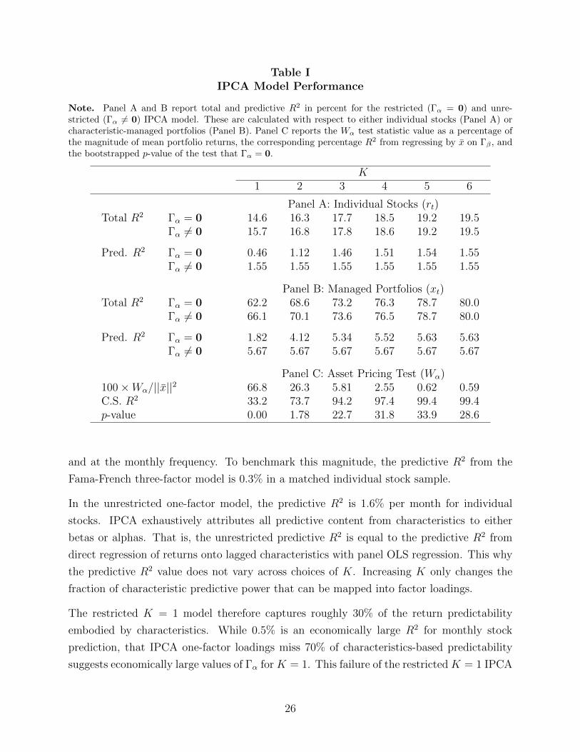
Table IIPCA Model Performance

Note. Panel A and B report total and predictive R2 in percent for the restricted (Γα = 0) and unre-stricted (Γα 6= 0) IPCA model. These are calculated with respect to either individual stocks (Panel A) orcharacteristic-managed portfolios (Panel B). Panel C reports the Wα test statistic value as a percentage ofthe magnitude of mean portfolio returns, the corresponding percentage R2 from regressing by x̄ on Γβ , andthe bootstrapped p-value of the test that Γα = 0.

K1 2 3 4 5 6

Panel A: Individual Stocks (rt)Total R2 Γα = 0 14.6 16.3 17.7 18.5 19.2 19.5

Γα 6= 0 15.7 16.8 17.8 18.6 19.2 19.5

Pred. R2 Γα = 0 0.46 1.12 1.46 1.51 1.54 1.55Γα 6= 0 1.55 1.55 1.55 1.55 1.55 1.55

Panel B: Managed Portfolios (xt)Total R2 Γα = 0 62.2 68.6 73.2 76.3 78.7 80.0

Γα 6= 0 66.1 70.1 73.6 76.5 78.7 80.0

Pred. R2 Γα = 0 1.82 4.12 5.34 5.52 5.63 5.63Γα 6= 0 5.67 5.67 5.67 5.67 5.67 5.67

Panel C: Asset Pricing Test (Wα)100×Wα/||x̄||2 66.8 26.3 5.81 2.55 0.62 0.59C.S. R2 33.2 73.7 94.2 97.4 99.4 99.4p-value 0.00 1.78 22.7 31.8 33.9 28.6

and at the monthly frequency. To benchmark this magnitude, the predictive R2 from the

Fama-French three-factor model is 0.3% in a matched individual stock sample.

In the unrestricted one-factor model, the predictive R2 is 1.6% per month for individual

stocks. IPCA exhaustively attributes all predictive content from characteristics to either

betas or alphas. That is, the unrestricted predictive R2 is equal to the predictive R2 from

direct regression of returns onto lagged characteristics with panel OLS regression. This why

the predictive R2 value does not vary across choices of K. Increasing K only changes the

fraction of characteristic predictive power that can be mapped into factor loadings.

The restricted K = 1 model therefore captures roughly 30% of the return predictability

embodied by characteristics. While 0.5% is an economically large R2 for monthly stock

prediction, that IPCA one-factor loadings miss 70% of characteristics-based predictability

suggests economically large values of Γα for K = 1. This failure of the restricted K = 1 IPCA

26

model is statistically borne out by the hypothesis test of Γα = 0 in Panel C. The test statistic,

Wα, is the sum of squared elements of Γα. To interpret the magnitude of the test statistic,

we report it as a percentage of squared average portfolio returns, 100×Wα/||x̄||2. The cross

section regression of x̄ on Γ̂β in equation (15), which quantifies the relative magnitude of

IPCA pricing errors for characteristic-managed portfolios, is equal to

C.S. R2 = 1−Wα/||x̄||2

and is also reported. For K = 1, 66.8% of cross section variation in average portfolio returns

is unexplained by IPCA, thus the test rejects Γα = 0 with a p-value below 0.1%.

When we allow for multiple IPCA factors, the gap between restricted and unrestricted models

shrinks rapidly. At K = 3, the total R2 for the restricted model is 17.7%, thus achieving

more than 99% of the explanatory power of the unrestricted model. The predictive R2 rises

to 1.5%, capturing 94% of all characteristics’ predictive content while imposing Γα = 0. The

magnitude of the test statistic drops dramatically, as the restricted K = 3 IPCA model

leaves only to 5.8% of variation in x̄ unexplained. The test fails to reject the null hypothesis

that Γα = 0 by a large margin (p-value of 22.7%). The results for K > 3 are quantitatively

similar.

This result says that, with K ≥ 3 factors, IPCA explains essentially all of the heterogeneity

in average stock returns associated with stock characteristics. It does so by identifying a

set of factors and associated loadings such that stocks’ expected returns align with their

exposures to systematic risk—without resorting to alphas to explain the predictive role of

characteristics. In other words, IPCA infers that characteristics are risk exposures, not

anomalies.

Note that, because IPCA is estimated from a least squares criterion, it directly targets total

R2. Thus the risk factors that IPCA identifies are optimized to describe the systematic risks

among stocks. They are by no means specialized to explain average returns, however, as

estimation does not directly target the predictive R2. Because conditional expected returns

are a small portion of total return variation (as evidenced by the 1.6% predictive R2 in

the unrestricted model), it is very well possible that a misspecified model could provide an

excellent description of risk yet a poor description of risk compensation. Evidently, this is

not the case for IPCA, as its risk factors indirectly produce an accurate description of risk

compensation across assets.

The asset pricing literature is accustomed to evaluating the performance of pricing factors

in explaining the behavior of test portfolios, such as the 5×5 size and value-sorted portfolios

27

of Fama and French (1993), as opposed to individual stocks. The behavior of portfolios

can differ markedly from individual stocks because a large amount of idiosyncratic stock

behavior is averaged out. As emphasized in Section 3.1.1, IPCA asset pricing tests can be

equivalently interpreted as tests of stocks or of a particular set of characteristic-managed

portfolios. In this spirit, Panel B of Table I evaluates fit measures for managed portfolios,

xt.10 With K = 3 factors, the total R2’s for the restricted and unrestricted models are 73.2%

and 73.6%, respectively. Indeed, systematic risk explains three-fourths of total variation in

portfolio returns. The reduction in noise via portfolio formation also improves predictive

R2’s to 5.3% and 5.7%, respectively.

5.3 Comparison with Observable Factors

The results in Table I compare the performance of IPCA across specification choices for

K and with or without imposition of asset pricing restrictions. We now compare IPCA to

leading alternative modeling approaches in the literature. The first includes models with pre-

specified observable factors. We consider models with K = 1, 3, 4, 5, or 6 observable factors.

The K = 1 model is the CAPM (using the CRSP value-weighted excess market return as

the factor), the K = 3 model is the Fama-French (1993) three-factor model that includes

SMB and HML (“FF3” henceforth) with the market. The K = 4 model is the Carhart

(1997, “FFC4”) model that adds MOM to the FF3 model. K = 5 is the Fama-French (2015,

“FF5”) five-factor model that adds RMW and CMA to the FF3 factors. Finally, we consider

a six-factor model (“FFC6”) that includes MOM alongside the FF5 factors.

The second set of alternatives are static latent factor models estimated with PCA. In this

approach, we consider one to six principal component factors from the panel of individual

stock returns.

We estimate all models in Table II restricting intercepts to zero. For IPCA, we do so

imposing Γα = 0. For the observable factor models, we estimate stock-by-stock time series

regressions via OLS omitting a constant. For static latent factor models, we estimate PCA

from uncentered stocked returns. This forces a stock’s average return to equal its static

factor loading times the factors’ time series average, exactly mirroring our estimation of the

10Fit measures for xt are

Total R2 = 1−

∑t

(xt − Γ̂α − Γ̂β f̂t

)′ (xt − Γ̂α − Γ̂β f̂t

)∑t x′txt

, Predictive R2 = 1−

∑t

(xt − Γ̂α − Γ̂βλ̂

)′ (xt − Γ̂α − Γ̂βλ̂

)∑t x′txt

.

28

Table IIIPCA Comparison With Observable Factors

Note. The table reports total and predictive R2 in percent and number of estimated parameters (Np) forthe restricted (Γα = 0) IPCA model (Panel A), for observable factor models (Panel B), and for static latentfactor models (Panel D). Observable factor models specifications are: K = 1 MKT-RF; K = 3 (MKT-RF,SMB,HML); K = 4 (MKT-RF,SMB,HML,MOM); K = 5 (MKT-RF,SMB,HML,RMW,CMA); K = 6(MKT-RF,SMB,HML,RMW,CMA,MOM). Panel C reports tests of the incremental explanatory power ofeach observable factor model with respect to the K = 3 IPCA model. Incremental total R2 is the percentageof total portfolio variation explained by observable factors after controlling for K = 3 IPCA. IncrementalC.S. R2 is the percentage of cross-sectional variation in average portfolio returns explained by observablefactors after controlling for K = 3 IPCA.

Test KAssets Statistic 1 3 4 5 6

Panel A: IPCArt Total R2 14.8 17.8 18.6 19.3 19.6

Pred. R2 0.47 1.42 1.47 1.50 1.51Np 671 2013 2684 3355 4026

xt Total R2 62.2 73.2 76.3 78.7 80.0Pred. R2 1.82 5.34 5.52 5.63 5.63Np 671 2013 2684 3355 4026

Panel B: Observable Factorsrt Total R2 11.9 18.9 20.9 21.9 23.7

Pred. R2 0.31 0.29 0.28 0.29 0.23Np 11452 34356 45808 57260 68712

xt Total R2 45.4 60.4 62.8 62.3 64.5Pred. R2 1.28 1.92 1.84 2.31 2.16Np 72 216 288 360 432

Panel C: Test of IPCA vs. Observable FactorsWΨ p-value 80.5 0.01 0.00 0.01 0.03Wλ p-value 0.01 0.00 0.00 0.00 0.00Incremental Total R2 0.02 0.71 1.78 1.01 2.04Incremental C.S. R2 0.56 2.09 2.13 2.12 2.16

Panel D: Principal Componentsrt Total R2 16.8 26.2 29.0 31.5 33.8

Pred. R2 < 0 < 0 < 0 < 0 < 0Np 13412 40236 53648 67060 80472

restricted IPCA model.11

11In calculating PCA, we confront the fact that the panel of returns is unbalanced. Therefore, we mustestimate PCA using an alternating least squares EM algorithm as described by Stock and Watson (2002b).

29

Table II reports the total and predictive R2 as well as the number of estimated parameters

(Np) for each model.12 For ease of comparison, Panel A report model fit results for IPCA

with Γα = 0.13 Panel B reports fits for the observable factor models (CAPM through FFC6).

In the analysis of individual stocks, observable factor models generally produce a slightly

higher total R2 than the IPCA specification using the same number of factors. For example,

at K = 3, FF3 achieves a 1.1 percentage point improvement in R2 relative to IPCA’s fit of

17.8%. To accomplish this, however, observable factors rely on vastly more parameters than

IPCA. The number of parameters in an observable factor model is equal to the number of

loadings, or Np = NK. For IPCA, the number of factors is the dimension of Γβ plus the

number of estimated factor realizations, or Np = LK + TK. In our sample of 11,452 stocks

with 72 instruments over 599 months, observable factor models therefore estimate 17 times

(≈ 11452/(72 + 599)) as many parameters as IPCA.14 In short, IPCA provides a similar

description of systematic risk in individual stock returns as the leading observable factors

while using almost 95% fewer parameters.

At the same time, IPCA provides a substantially more accurate description of stocks’ risk

compensation than observable factor models, as evidenced by the predictive R2. Observable

factor models’ predictive power never rises beyond 0.3% for any specification, only a fifth of

the 1.4% predictive R2 from IPCA with K = 3.

Among xt, observable factor models’ total R2 suffers in comparison to IPCA. At K = 3,

IPCA explains 73.2% of total portfolio return variation while FF5 explains 62.3%. IPCA

(K = 3) more than doubles the predictive R2 of FF5, at 5.3% versus 2.3%. When test assets

are managed portfolios, IPCA dominates in its ability to describe systematic risks as well as

cross-sectional differences in average returns.

As a practical matter, this means that PCA estimation for individual stocks bears a high computationalcost. It also highlights the computational benefit of IPCA, which side steps the unbalanced panel problemby parameterizing betas with characteristics and, as a result, is estimated from managed portfolios that canalways be constructed to have no missing data.

12The R2’s for alternative models are defined analogously to those of IPCA. In particular, for individualstocks they are

Total R2 = 1−

∑i,t

(ri,t − β̂if̂t

)2∑i,t r

2i,t

,Predictive R2 = 1−

∑i,t

(ri,t − β̂iλ̂

)2∑i,t r

2i,t

,

and are similarly adapted for managed portfolios xt. In all cases, model fits are based on exactly matchedsamples with IPCA.

13These differ minutely from Table I results because we drop some stock-month observations for the sakeof estimating the observable factor models—see footnote 14.

14Because we require at least 60 non-missing months to compute observable factor betas, we filter outslightly more than a thousand stocks compared to the sample used in Table I. As a result, statistics inTables I and II can differ minutely.

30

Panel C formally compares of each observable factor model versus IPCA (with K = 3) using

the tests from Section 4.2. We can easily reject the null of no additional explanatory power

from observable factors for all models except the CAPM. Despite this rejection, the incre-

mental benefits of observable factors have small economic magnitudes. The “Incremental

Total R2” row describes the fraction of variation in xt explained by each observable factor

model after controlling for the three-factor IPCA specification.15 After IPCA explains 73.2%

of the panel variation in xt, observable factors explain at most another 2.0% (FFC6).16 We

likewise report the “Incremental C.S. R2,” which describes the fraction of variation in x̄ de-

scribed by observable factor loadings after controlling for IPCA three-factor loadings. IPCA

explains 97.4% of the heterogeneity in x̄, and FFC6 captures an additional 2.1%. In either

calculation, the incremental contribution of observable factors is economically small.

In Panel D we report the performance of static latent factor models estimated with PCA.

Naturally, in this panel, we report only the analysis for individual stocks (PCA on xt is

identical to IPCA). For all K, the total R2 exceeds that of IPCA and observable factor mod-

els. This is expected as PCA directly selects factors and loadings to maximize the explained

variance of stock returns and is the least constrained estimator of the three approaches. This

is evident in its parameter count, Np = NK + TK, which exceeds even that of observable

factor models.

While PCA optimizes the in-sample description of systematic risk, it provides a dismal

description of risk compensation. The static PCA loadings provide such a poor description

of expected returns that the predictive R2 is negative for every K. In other words, a static

return forecast of zero for all stocks is a better prediction than using the estimated risk

loadings from PCA.

5.4 Out-of-sample Comparisons

Thus far, the comparison of IPCA and alternatives has been based on in-sample estimates.

That is, IPCA and PCA factors and loadings are estimated from the full panel of stock

returns, and observable factor loadings are estimated from the full time series. Next we

analyze out-of-sample fits from IPCA and observable factor models. Due to the poor in-

sample predictive performance of PCA, we exclude it from out-of-sample comparisons.

15Let R2IPCA denote total R2 for xt using the IPCA model. Let R2

A denote the regression of IPCA residualson observable factors in equation (20). The incremental total R2 due to observable factors as (1−R2

IPCA)R2A.

16The incremental R2 is non-monotonic inK because observable factor specifications are non-nested. FFC4and FFC6 include MOM, while FF5 does not. The size of the non-monotonicity indicates that momentumis the most important observable factor in terms of incremental total R2.

31

Table IIIOut-of-sample Fits

Note. The table reports out-of-sample total and predictive R2 in percent.

Test KAssets Statistic 1 3 4 5 6

Panel A: IPCArt Total R2 12.2 14.1 14.6 15.1 15.7

Pred. R2 0.40 0.48 0.50 0.50 0.50

xt Total R2 50.5 51.7 51.9 52.7 53.4Pred. R2 1.75 3.35 3.40 3.46 3.42

Panel B: Observable Factorsrt Total R2 8.33 9.65 8.38 7.74 6.55

Pred. R2 0.26 0.30 0.17 0.21 0.11

xt Total R2 37.5 49.6 52.8 51.4 54.4Pred. R2 1.33 2.31 2.33 2.87 2.81

To construct out-of-sample fit measures, we use recursive backward-looking estimation and

track the post-estimation performance of estimated models. In particular, in every month

t ≥ T/2, we use all data through t to estimate the IPCA model and save the estimates

Γ̂β,t and λ̂t.17 Then, based on equation (14), we calculate the out-of-sample realized factor

return at t+ 1 as f̂t+1,t =(

Γ̂′β,tΓ̂β,t

)−1

Γ̂′β,txt+1. That is, IPCA factor returns at t+ 1 may be

calculated with individual stock weights(

Γ̂′β,tΓ̂β,t

)−1 (Γ̂′β,tZ

′t

)that require no information

beyond time t, just like the portfolio sorts used to construct observable factors.

The out-of-sample total R2 compares rt+1 to ZtΓ̂β,tf̂t+1,t and xt+1 to Γ̂β,tf̂t+1,t. The out-

of-sample predictive R2 is defined analgously, replacing f̂t+1,t with λ̂t. Fit measures for

observable factor models are the same with the difference that factor realizations at t+ 1 do

not need to be constructed.

Table III reports out-of-sample R2 statistics. The main conclusion from the table is that the

strong performance of IPCA, both in absolute terms and relative to leading observable factor

models, is not merely an in-sample phenomenon driven by statistical overfit. IPCA delivers

nearly the same out-of-sample total R2 that it achieves in-sample. And while the predictive

R2 is noticeably reduced, it remains economically large and outperforms the predictions from

observable factors, for both individual stocks and managed portfolios.

17Hence, our out-of-sample period begins in mid-1989.

32

Table IVOut-of-Sample Factor Portfolio Efficiency

Note. The table reports out-of-sample annualized Sharpe ratios for individual factors (“univariate”) andfor the mean-variance efficient portfolio of factors in each model (“tangency”).

K1 2 3 4 5 6

Panel A: IPCAUnivariate 0.64 0.83 0.58 0.37 0.47 0.14Tangency 0.64 0.96 1.31 1.57 1.75 2.15

Panel B: Observable FactorsUnivariate 0.49 0.19 0.25 0.49 0.48 0.42Tangency 0.49 0.35 0.52 0.68 0.91 0.96

5.5 Factor Efficiency

Zero intercepts in a factor pricing model are equivalent to multivariate mean-variance ef-

ficiency of the factors. This fact is the basis for the Gibbons, Ross, and Shanken (1989)

alpha test and bears a close association with our Wα test. The evidence thus far indicates

that IPCA describes expected asset returns more accurately than competing factor models

both in-sample and out-of-sample, suggesting that IPCA factors achieve higher multivariate

efficiency than competitors. In this section, we directly investigate factor efficiency in terms

of annualized Sharpe ratios.

Kozak, Nagel, and Santosh (forthcoming) emphasize that higher-order principal components

of “anomaly” portfolios tend to be overfit and generate unreasonably high in-sample Sharpe

ratios. In light of this, we focus our analysis on out-of-sample IPCA factor returns. We report

univariate Sharpe ratios to describe individual factor efficiency. To describe multivariate

efficiency, we report the tangency portfolio Sharpe ratio for a group of factors. We calculate

out-of-sample factor returns following the same recursive estimation approach from Section

5.3. The tangency portfolio return for a set of factors is also constructed on a purely out-

of-sample basis by using the mean and covariance matrix of estimated factors through t and

tracking the post-formation t+ 1 return.

Out-of-sample IPCA Sharpe ratios are shown in Panel A of Table IV. The kth column reports

the univariate Sharpe ratio for factor k as well as the tangency Sharpe ratio based on factors

1 through k. For comparison, we report Sharpe ratios of observable factor models in Panel

33

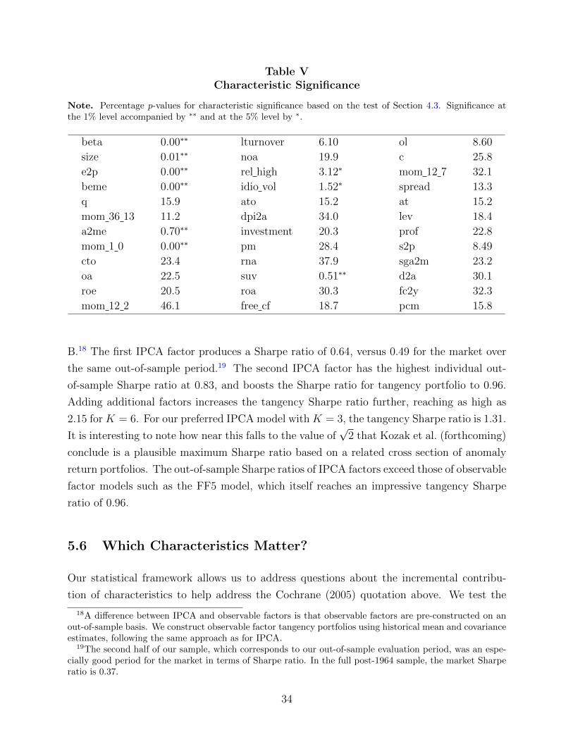
Table VCharacteristic Significance

Note. Percentage p-values for characteristic significance based on the test of Section 4.3. Significance atthe 1% level accompanied by ∗∗ and at the 5% level by ∗.

beta 0.00∗∗ lturnover 6.10 ol 8.60

size 0.01∗∗ noa 19.9 c 25.8

e2p 0.00∗∗ rel high 3.12∗ mom 12 7 32.1

beme 0.00∗∗ idio vol 1.52∗ spread 13.3

q 15.9 ato 15.2 at 15.2

mom 36 13 11.2 dpi2a 34.0 lev 18.4

a2me 0.70∗∗ investment 20.3 prof 22.8

mom 1 0 0.00∗∗ pm 28.4 s2p 8.49

cto 23.4 rna 37.9 sga2m 23.2

oa 22.5 suv 0.51∗∗ d2a 30.1

roe 20.5 roa 30.3 fc2y 32.3

mom 12 2 46.1 free cf 18.7 pcm 15.8

B.18 The first IPCA factor produces a Sharpe ratio of 0.64, versus 0.49 for the market over

the same out-of-sample period.19 The second IPCA factor has the highest individual out-

of-sample Sharpe ratio at 0.83, and boosts the Sharpe ratio for tangency portfolio to 0.96.

Adding additional factors increases the tangency Sharpe ratio further, reaching as high as

2.15 for K = 6. For our preferred IPCA model with K = 3, the tangency Sharpe ratio is 1.31.

It is interesting to note how near this falls to the value of√

2 that Kozak et al. (forthcoming)

conclude is a plausible maximum Sharpe ratio based on a related cross section of anomaly

return portfolios. The out-of-sample Sharpe ratios of IPCA factors exceed those of observable

factor models such as the FF5 model, which itself reaches an impressive tangency Sharpe

ratio of 0.96.

5.6 Which Characteristics Matter?

Our statistical framework allows us to address questions about the incremental contribu-

tion of characteristics to help address the Cochrane (2005) quotation above. We test the

18A difference between IPCA and observable factors is that observable factors are pre-constructed on anout-of-sample basis. We construct observable factor tangency portfolios using historical mean and covarianceestimates, following the same approach as for IPCA.

19The second half of our sample, which corresponds to our out-of-sample evaluation period, was an espe-cially good period for the market in terms of Sharpe ratio. In the full post-1964 sample, the market Sharperatio is 0.37.

34

Table VIIPCA Fits Excluding Insignificant Instruments

Note. IPCA percentage R2 at the individual stock level including only the seven characteristics from TableV that are significant at the 1% level.

K

1 2 3 4 5 6

Total R2 Γα = 0 14.3 15.9 17.2 17.9 18.5 18.7

Γα 6= 0 15.5 16.2 17.3 18.0 18.5 18.7

Pred. R2 Γα = 0 0.47 1.38 1.56 1.58 1.62 1.61

Γα 6= 0 1.61 1.61 1.61 1.61 1.61 1.61

statistical significance of an individual characteristic while simultaneously controlling for all

other characteristics. Each characteristic enters the beta specification through two rows of

Γβ matrix: one row corresponding to the average level of the characteristic and the other to

deviations around this level. A characteristic is irrelevant to the asset pricing model is all Γβ

elements in these two rows are zero. Our tests of characteristic l’s significance is based on

the Wβ statistic of Section 4.3 which measures the distance of these two Γβ rows from zero.

Table V reports p-values for the significance of each characteristic based on this test. Of the

36 characteristics in our sample, only seven are significant at the 1% level: market beta, size,

earnings-to-price, book-to-market, assets-to-market, short-term reversal, and unexplained

volume. Two more, price relative to its trailing 52-week high and idiosyncratic volatility, are

significant at the 5% level.

The insignificance of so many characteristics begs the question of whether the small subset

of significant characteristics produces a factor model with similar explanatory power to the

36 characteristics data set. Table VI repeats the IPCA model fit analysis of Table I but

instead uses only the seven characteristics that are significant at the 1% level. The seven-

characteristic model overall performs very similarly to the model with all 36 characteristics.

For K = 3, the total R2 in the Γα = 0 model is 17.2% and 17.8% for seven and 36 char-

acteristics, respectively. And the predictive R2 improves slightly in the seven-characteristic

model from 1.42% to 1.56%.

The results of Table I show that characteristics align with expected returns through their

association with risk exposures rather than alphas. Additionally, Table VI suggests that

the success of IPCA is obtainable using only a few characteristics, with the others being

statistically irrelevant for the model’s fit.

35

5.6.1 Static or Dynamic Loadings?

Our definition of zi,t splits each characteristic into two instruments: its mean and its time

series deviation from the mean. We next analyze the relative contribution of these two

components to the return factor model. In addition to our main specification in which

zi,t = (c̄′i, c′i,t − c̄′i)′, we consider three nested variations of the IPCA model. The first sets

instruments equal the total characteristic value, zi,t = ci,t. This is equivalent to imposing

that the Γβ coefficients corresponding to c̄i and ci,t − c̄i are equal, and helps answer the

question “Do the level and variation in characteristics contribute different information to

factor loadings.” If this specification performs as well as our main specification, then level

and variation enter βi,t equally and there is no need to split them.

The second variation sets instruments equal to the mean characteristic value, zi,t = c̄i. This

is equivalent to setting Γβ coefficients on to ci,t− c̄i equal to zero. By testing this against our

main specification we address the question, “Is a static factor model sufficient for describing

returns?,” in which case the benefits of characteristics shown in our preceding results arise

from their ability to better differentiate loadings across assets rather than over time. The

third variation asks the complementary question, “Is time series variation in characteristics

the primary contributor to IPCA success?” In this case we set instruments equal to the

deviation value only, zi,t = ci,t − c̄i, and fix coefficients on c̄i to zero.

Because these comparisons can be formulated as restrictions on rows of Γβ, the model com-

parison test in Section 4.3 can be used to conduct formal statistical inference for whether

our main split-characteristic specification significantly improves over each of the three nested

variations.20

Table VII reports model fits for each specification. In terms of total R2, the nested variation

that is closest to our main specification for K = 3 is that using characteristic means, zi,t = c̄i.

It produces a total R2 of 16.6%, versus 17.7% in the main model. This suggests that, for the

purposes of describing asset riskiness, the unconditional levels of characteristics are nearly

as informative as splitting it into its level and variation.

However, the predictive R2 results show that temporal variation around the mean is the most

important characteristic component for describing risk compensation. Conditional expected

return estimates from time series variation alone describe 1.2% of total return variance,

20Goyal (2012) notes that “In practice, one almost always employs firm characteristics that vary overtime. There are relatively few analytical results in the literature for the case dealing with time-varyingcharacteristics.” The tests we describe in this section provide a means of investigating the role of time-varying characteristics in a fully formulated statistical setting.

36

Table VIIStatic Versus Dynamic Loadings

Note. Percentage R2 from IPCA specifications based on either total characteristics, time series meancharacteristics, deviations from their mean, or both.

Total R2 Predictive R2

K c c̄ c− c̄ c̄, c− c̄ c c̄ c− c̄ c̄, c− c̄1 13.9 14.1 12.8 14.6 0.33 0.31 0.41 0.46

2 15.1 15.8 14.4 16.3 0.41 0.35 1.08 1.12

3 16.1 16.6 15.2 17.7 0.43 0.41 1.21 1.46

4 16.9 17.1 15.8 18.5 0.46 0.70 1.21 1.51

5 17.6 17.4 16.2 19.2 0.46 0.70 1.21 1.54

6 18.2 17.6 16.5 19.5 0.59 0.71 1.23 1.55

versus 1.5% from the main split-characteristic specification and 0.4% for the c̄i specification.

Lastly, the statistical test rejects all three nested variations in favor of the more general split-

characteristic specification with p-values below 1%.21 This is true for all K. In summary,

the data significantly prefer a dynamic factor model over a static one, and the variation in

characteristics across assets and over time contribute differently (and both significantly) to

the specification of betas.

6 Conclusion

Our primary conclusions are three-fold. First, by estimating latent factors as opposed to

relying on pre-specified observable factors, we find a three-factor model that is successfully

describes riskiness of stock returns (by explaining realized return variation) and risk com-

pensation (by explaining cross section differences in average returns). We show that there

are no significant anomaly intercepts associated with a large collection stock characteristics,

and instead show that the differences in average returns across stocks align with differences

in exposures to our three factors.

Second, our three-factor model outperforms leading observable factor models, such as the

Fama-French five-factor model, in delivering small pricing errors. This is true in-sample

and out-of-sample. Our factors also achieve a higher level of out-of-sample mean-variance

efficiency than alternative models.

21We omit percentage p-values from the table because as they all are zero to two decimal places.

37

Third, only a small subset of the stock characteristics are responsible for the empirical success

of our approach. The remaining 80% of the characteristics in our sample are statistically

irrelevant to our factor model. Our tests conclude that the 20% of characteristics that are

significant add value by better identifying latent factor loadings, and show no statistical

evidence of generating anomaly alphas.

The key to isolating a successful factor model is incorporating information from stock char-

acteristics into the estimation of factor loadings. We propose a model in which risk loadings

are partially dependent on observable asset characteristics. We propose a new method,

instrumental principal components analysis (IPCA), which treats characteristics as instru-

mental variables for estimating dynamic loadings. The estimator is as easy to work with as

standard PCA while allowing the researcher to bring information beyond just returns into

estimation of latent factors and betas. We introduce a set of statistical asset pricing tests

that offer a new research protocol for evaluating hypotheses about patterns in asset returns.

When a research encounters a new anomaly characteristic, they should test in a multivari-

ate setting against the large body of previously studied characteristics via IPCA. In doing

so, the researcher can draw inferences regarding the incremental explanatory power of the

proposed characteristic after controlling for the extant gamut. And if the characteristic does

contribute significantly to the return model, the research can then test whether it contributes

as a risk factor loading or as an anomaly alpha. Thus, the researcher need no longer asks the

narrow question, “Is my proposed characteristic/return association explained by a specific

set of pre-specified factors,” and instead can ask “Does there exist any set of factors that

explains the observed characteristic/return pattern?”

38

References

Asness, C. S., A. Frazzini, and L. H. Pedersen (2014): “Quality Minus Junk,” Dis-

cussion paper, AQR.

Carhart, M. (1997): “On Persistence in Mutual Fund Performance,” Journal of Finance,

52(1), 57–82.

Chamberlain, G., and M. Rothschild (1983): “Arbitrage, Factor Structure, and Mean-

Variance Analysis on Large Asset Markets,” Econometrica, 51(5), 1281–304.

Chordia, T., A. Goyal, and J. Shanken (2015): “Cross-Sectional Asset Pricing with

Individual Stocks: Betas versus Characteristics,” Working papers, Emory Goizueta and

Swiss Finance Institute.

Cochrane, J. (2005): Asset Pricing. Princeton University Press, second edn.

Connor, G., and R. A. Korajczyk (1988): “Risk and return in an equilibrium APT :

Application of a new test methodology,” Journal of Financial Economics, 21(2), 255–289.

Connor, G., and R. A. Korajczyk (1989): “An Intertemporal Equilibirum Beta Pricing

Model,” Review of Financial Studies, 2(3), 373–392.

(1993): “A Test for the Number of Factors in an Approximate Factor Model,”

Journal of Finance, 48(4), 1263–91.

Daniel, K., and S. Titman (1997): “Evidence on the Characteristics of Cross Sectional

Variation in Stock Returns,” Journal of Finance, 52(1), 1–33.

Daniel, K., S. Titman, et al. (2012): “Testing factor-model explanations of market

anomalies,” Critical Finance Review, 1(1), 103–139.

Fama, E., and K. French (1993): “Common risk factors in the returns on stocks and

bonds,” Journal of Financial Economics, 33(1), 3–56.

Fama, E., and J. MacBeth (1973): “Risk, Return, and Equilibrium: Empirical Tests,”

Journal of Political Economy, 81(3), 607–36.

Fama, E. F., and K. R. French (2015): “A five-factor asset pricing model,” Journal of

Financial Economics, 116(1), 1–22.

Fan, J., Y. Liao, and W. Wang (2016): “Projected principal component analysis in

factor models,” Ann. Statist., 44(1), 219–254.

39

Ferson, W., and C. Harvey (1991): “The Variation of Economic Risk Premiums,”

Journal of Political Economy, 99(2), 385–415.

Freyberger, J., A. Neuhierl, and M. Weber (2017): “Dissecting Characteristics Non-

parametrically,” Working papers, University of Wisconsin and Notre Dame and Chicago

Booth.

Gibbons, M. R., S. Ross, and J. Shanken (1989): “A Test of the Efficiency of a Given

Portfolio,” Econometrica, 57(5), 1121–52.

Goncalves, S., and L. Kilian (2004): “Bootstrapping autoregressions with conditional

heteroskedasticity of unknown form,” Journal of Econometrics, 123(1), 89–120.

Goyal, A. (2012): “Empirical cross-sectional asset pricing: a survey,” Financial Markets

and Portfolio Managament, 26, 3–38.

Hansen, L. P., and S. F. Richard (1987): “The Role of Conditioning Information in

Deducing Testable Restrictions Implied by Dynamic Asset Pricing Models,” Econometrica,

55(3), 587–613.

Kelly, B. T., S. Pruitt, and Y. Su (2017): “Instrumented Principal Component Anal-

ysis,” Working papers, Chicago Booth and ASU WP Carey.

Kozak, S., S. Nagel, and S. Santosh (2017): “Shrinking the Cross-Section,” Discussion

paper, Michigan Ross and Chicago Booth and Maryland Smith.

(forthcoming): “Interpreting Factor Models,” Journal of Finance.

Lewellen, J. (2015): “The Cross-section of Expected Stock Returns,” Critical Finance

Review, 4, 1–44.

Lewellen, J., S. Nagel, and J. Shanken (2010): “A skeptical appraisal of asset pricing

tests,” Journal of Financial economics, 96(2), 175–194.

Light, N., D. Maslov, and O. Rytchkov (2017): “Aggregation of Information About

the Cross Section of Stock Returns: A Latent Variable Approach,” Review of Financial

Studies, 30(4), 1339–1381.

Roll, R. (1977): “A critique of the asset pricing theory’s tests Part I: On past and potential

testability of the theory,” Journal of Financial Economics, 4(2), 129–176.

Rosenberg, B. (1974): “Extra-Market Components of Covariance in Security Returns,”

Journal of Financial and Quantitative Analysis, 9(2), 263–274.

40

Ross, S. A. (1976): “The Arbitrage Theory of Capital Asset Pricing,” Journal of Economic

Theory, 13, 341–360.

Stock, J. H., and M. W. Watson (2002a): “Forecasting Using Principal Components

from a Large Number of Predictors,” Journal of the American Statistical Association,

97(460), 1167–1179.

(2002b): “Macroeconomic Forecasting Using Diffusion Indexes,” Journal of Busi-

ness & Economic Statistics, 20(2), 147–62.

41

Internet Appendix

A Bootstrap Test Monte Carlo

This appendix investigates the finite sample behavior of our test for the null hypothesis

H0 : Γα = 0. Our analysis focuses on assessing the size of the test (rejection rates under the

null) and power of the test (rejection rates under the alternative).

We simulate data according to the following general model:

rt = Zt−1Γακ+ (Zt−1Γβ + νt)Ft + ηt.

We assume use cross sections of N = 500, 5000, or 25000 assets with T = 100 or 1000

monthly observations. We allow for K = 3 or 5 factors, and consider sets of L = 10 or 20

instruments.

We draw Γβ as a random orthonormal matrix. To do this, we draw an L × K matrix of

normals, M , and set Γβ = MM−1C for MC the Cholesky of M ′M . We draw Zt as an N × L

matrix of standard normals. We allow betas to possess a purely unobservable component,

νt, which is an N ×K array of normals, with the variance parameter chosen such that 50%

of the variation of βt−1 ≡ Zt−1Γβ + νt is due to νt.

Idiosyncratic returns, ηt, are drawn as a N × 1 array of normals with time-varying volatility.

In particular, the conditional variance ηt is log-normally distributed with its own variance

chosen such that on average 15% of return variance is systematic and 85% is idiosyncratic.

By incorporating heteroskedasticity akin to that in the data, we can assess the usefulness of

the wild bootstrap in conducting inference.

Γα is a random normal vector that is orthogonal to Γβ. In particular, we draw a L×1 vector

of normals, Y , and set Γα = (IL − Γβ(Γ′βΓβ)−1Γ′β)Y κ. Factor realizations ft are drawn as a

K × 1 vector of normals.

The distance-from-null is controlled by κ. When κ = 0 the model embodies the null hypoth-

esis that Γα = 0. For κ > 0, data is generated under the alternative. We consider three

values of κ > 0 such that when κ = κx, Zt−1Γακx drives about x× 0.25% of the variation in

returns.

In every simulated data set, we calculate the Wα statistic and perform the bootstrap proce-

dure of Section 4.1 to arrive at a p-value. We also consider a variation on our test that uses

42

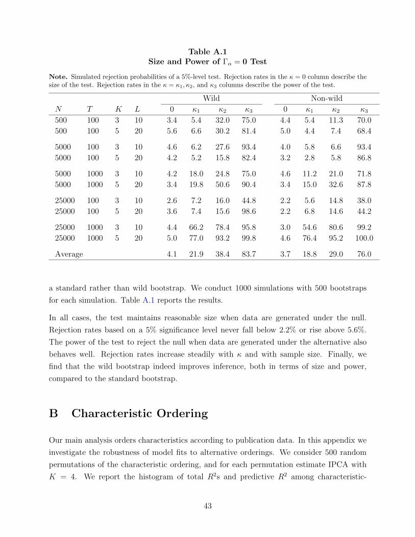
Table A.1Size and Power of Γα = 0 Test

Note. Simulated rejection probabilities of a 5%-level test. Rejection rates in the κ = 0 column describe thesize of the test. Rejection rates in the κ = κ1, κ2, and κ3 columns describe the power of the test.

Wild Non-wild

N T K L 0 κ1 κ2 κ3 0 κ1 κ2 κ3

500 100 3 10 3.4 5.4 32.0 75.0 4.4 5.4 11.3 70.0

500 100 5 20 5.6 6.6 30.2 81.4 5.0 4.4 7.4 68.4

5000 100 3 10 4.6 6.2 27.6 93.4 4.0 5.8 6.6 93.4

5000 100 5 20 4.2 5.2 15.8 82.4 3.2 2.8 5.8 86.8

5000 1000 3 10 4.2 18.0 24.8 75.0 4.6 11.2 21.0 71.8

5000 1000 5 20 3.4 19.8 50.6 90.4 3.4 15.0 32.6 87.8

25000 100 3 10 2.6 7.2 16.0 44.8 2.2 5.6 14.8 38.0

25000 100 5 20 3.6 7.4 15.6 98.6 2.2 6.8 14.6 44.2

25000 1000 3 10 4.4 66.2 78.4 95.8 3.0 54.6 80.6 99.2

25000 1000 5 20 5.0 77.0 93.2 99.8 4.6 76.4 95.2 100.0

Average 4.1 21.9 38.4 83.7 3.7 18.8 29.0 76.0

a standard rather than wild bootstrap. We conduct 1000 simulations with 500 bootstraps

for each simulation. Table A.1 reports the results.

In all cases, the test maintains reasonable size when data are generated under the null.

Rejection rates based on a 5% significance level never fall below 2.2% or rise above 5.6%.

The power of the test to reject the null when data are generated under the alternative also

behaves well. Rejection rates increase steadily with κ and with sample size. Finally, we

find that the wild bootstrap indeed improves inference, both in terms of size and power,

compared to the standard bootstrap.

B Characteristic Ordering

Our main analysis orders characteristics according to publication data. In this appendix we

investigate the robustness of model fits to alternative orderings. We consider 500 random

permutations of the characteristic ordering, and for each permutation estimate IPCA with

K = 4. We report the histogram of total R2s and predictive R2 among characteristic-

43

Figure A.1: Histograms of R2 Across Characteristic Orderings

Note. Total and predicted R2 among characteristic-managed portfolios (xt) in 500 random permutations ofthe characteristic ordering. The results from publication ordering in our main analysis are shown as a blackbar.

0.7 0.72 0.74 0.76 0.780

0.05

0.1

0.15

0.2

0.25

0.3PublicationRandom

0.02 0.03 0.04 0.05 0.06 0.070

0.05

0.1

0.15

0.2

0.25PublicationRandom

managed portfolios (xt) in Figure A.1. The results indicate that the total R2 is very stable

across ordering and ranges between 70% and 80%, versus 76.3% in our main analysis. The

predictive R2 ranges from 2.5% to 6.5%, with a modal value almost exactly equal to the

5.5% value in our main analysis.

44