Discussion paper

FOR 1 2010ISSN: 1500-4066JANUARY 2010

INSTITUTT FOR FORETAKSØKONOMI

DEPARTMENT OF FINANCE AND MANAGEMENT SCIENCE

Some aspects of random utility, ekstreme value theory and multinomial logit models

BYJONAS ANDERSSON AND JAN UBØE

Some aspects of random utility, extreme value theory and

multinomial logit models

Jonas Andersson and Jan Ubøe

Norwegian School of Economics and Business Administration

Helleveien 30, N5045 Bergen, Norway

January 15, 2010

Abstract

In this paper we give a survey on some basic ideas related to random utility, extreme

value theory and multinomial logit models. These ideas are well known within the field of

spatial economics, but do not appear to be common knowledge to researchers in probability

theory. The purpose of the paper is to try to bridge this gap.

Keywords: Random utility theory, extreme value theory, multinomial logit models, entropy.

1 Introduction

Statisticians and probabilists are in general familiar with models of discrete dependent variables.

The multinomial logit model, see, e.g., McFadden (1972), as an example, captures how a discrete

dependent variable is affected by a number of covariates. In many applications of such models,

the aim is to model the mechanism behind how individuals are chosing among a finite number

of alternatives. One example is in which city a person chooses to settle down and what factors

are affecting this choice (McFadden et al., 1978). Introductions to the field of discrete choice

models can be found in Dagsvik (2000) and Ben-Akiva and Lerman (1993). The latter of those

focuses in particular on how the theory is applied to travel demand.

What many statisticians and probabilists are not so familiar with is that such models are nat-

urally arising from random utility theory which is a common way for economists to analyze

the economics of discrete choice, see, e.g. Manski (1977). With some behavourial assumptions

1

on how choices are made, a multinomial logit model arises which can then be fitted to ob-

served data. Compared to many other fields in economics there is thus an unusually direct and

mathematically stringent link between the economic theory and the statistical model used to

operationalize it.

In this paper we review how this occurs. Furthermore, and perhaps more interestingly, we discuss

whether the behavioural assumptions are modest or restrictive. The assumption, very often

made, that random utility is Gumbel distributed is at first sight seemingly made purely to make

the transition from the economic theory to the statistical model mathematically convenient. It

can, however, be shown that there is considerably more depth to this transition and that the

assumption of Gumbel distributed random utility is not as restrictive as it might first appear.

It can nevertheless also be shown that the generality is limited to distributions with a particular

tail behaviour. Since the choices are made based on maximizing random utility we consider this

from the perspective of extreme value theory, see, e.g., De Haan and Ferreira (2006).

The sequel of the paper is structured as follows. Section 2 presents the principle of random

utility maximization and how it leads to the multinomial logit model. Furthermore, it discusses

how and in what circumstances breaches of the assumption of Gumbel distributed random utility

is irrelevant for the results. In Section 3, other arguments, in addition to random utility theory,

also leading to the multinomial logit model, are reviewed. A real world application with shipping

data, originally presented in Ubøe et al. (2009), is revisited in Section 4 and it is argued that a

model that corresponds to a Gumbel distributed random utility is empirically plausible. Some

concluding remarks closes the paper.

2 Random utility maximization

Consider a discrete set S = {S1, . . . , Sn} of objects which we will call the choice set. A large

number of independent agents want to choose an object each from S. Each object Si has a

deterministic utility vi which is common for all agents. In addition each object has a random

utility εi. The εi-s are IID random variables drawn from a distribution which is common for all

objects and all agents. Each agent computes

Ui = vi + εi i = 1, . . . , n (1)

2

and chooses the object with the largest total utility. The basic problem in random utility theory

is to compute the probabilities

pi = P (An agent chooses object nr i) (2)

If we assume that εi has a continuous distribution and use independence, these probabilities can

be computed as follows:

pi = P (An agent chooses object nr i) = P (Uj ≤ Ui,∀j 6= i)

= P (ε1 ≤ vi − v1 + εi, . . . , εi−1 ≤ vi − vi−1 + εi, εi+1 ≤ vi − vi+1 + εi,

. . . , εn ≤ vi − vn + εi)

=∫ ∞−∞

n∏j=1j 6=i

P (εj ≤ vi − vj + x)fε(x)dx (3)

In principle this is straightforward to compute for most distributions. The problem, however,

is that in many applications of this theory n is very large; n > 104 is common, and in special

cases, e.g., image reconstruction, n > 108. We then need to rewrite (3) to be able to carry out

the computations.

As a first step let us assume that ε has a Gumbel distribution with parameters µ = 0, β = 1,

i.e., a distribution with cumulative distribution function

Fε(x) = P (ε ≤ x) = ee−x

In that particular case we get

pi = P (An agent chooses object nr i) =∫ ∞−∞

n∏j=1j 6=i

P (Uj ≤ vi − vj + x)fε(x)dx

=∫ ∞−∞

n∏j=1j 6=i

e−evj−vi−x

e−xe−e−xdx =

∫ ∞0

n∏j=1j 6=i

e−evj−viue−udu

=∫ ∞

0e−(1+

Pnj=1j 6=i

evj−vi )u

du =1

1 +∑n

j=1j 6=i

evj−vi=

evi∑nj=1 e

vj(4)

3

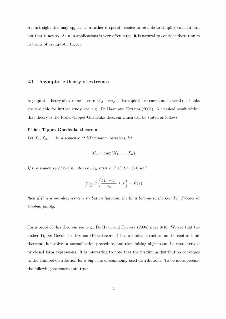
At first sight this may appear as a rather desperate choice to be able to simplify calculations,

but that is not so. As n in applications is very often large, it is natural to consider these results

in terms of asymptotic theory.

2.1 Asymptotic theory of extremes

Asymptotic theory of extremes is currently a very active topic for research, and several textbooks

are available for further study, see, e.g., De Haan and Ferreira (2006). A classical result within

that theory is the Fisher-Tippet-Gnedenko theorem which can be stated as follows:

Fisher-Tippet-Gnedenko theorem

Let X1, X2, . . . be a sequence of IID random variables, let

Mn = max{X1, . . . , Xn}

If two sequences of real numbers an, bn exist such that an > 0 and

limn→∞

P

(Mn − bn

an≤ x

)= F (x)

then if F is a non-degenerate distribution function, the limit belongs to the Gumbel, Frechet or

Weibull family.

For a proof of this theorem see, e.g., De Haan and Ferreira (2006) page 3-10. We see that the

Fisher-Tippet-Gnedenko theorem (FTG-theorem) has a similar structure as the central limit

theorem. It involves a normalization procedure, and the limiting objects can be characterized

by closed form expressions. It is interesting to note that the maximum distribution converges

to the Gumbel distribution for a big class of commonly used distributions. To be more precise,

the following statements are true:

4

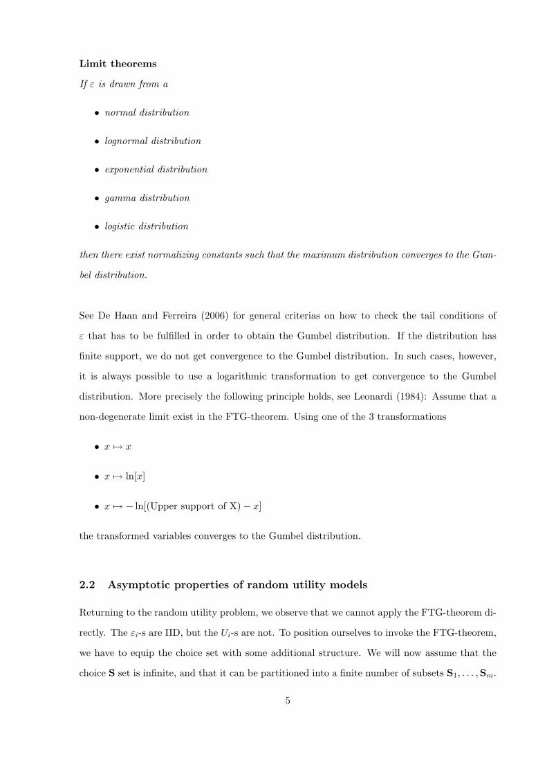
Limit theorems

If ε is drawn from a

• normal distribution

• lognormal distribution

• exponential distribution

• gamma distribution

• logistic distribution

then there exist normalizing constants such that the maximum distribution converges to the Gum-

bel distribution.

See De Haan and Ferreira (2006) for general criterias on how to check the tail conditions of

ε that has to be fulfilled in order to obtain the Gumbel distribution. If the distribution has

finite support, we do not get convergence to the Gumbel distribution. In such cases, however,

it is always possible to use a logarithmic transformation to get convergence to the Gumbel

distribution. More precisely the following principle holds, see Leonardi (1984): Assume that a

non-degenerate limit exist in the FTG-theorem. Using one of the 3 transformations

• x 7→ x

• x 7→ ln[x]

• x 7→ − ln[(Upper support of X)− x]

the transformed variables converges to the Gumbel distribution.

2.2 Asymptotic properties of random utility models

Returning to the random utility problem, we observe that we cannot apply the FTG-theorem di-

rectly. The εi-s are IID, but the Ui-s are not. To position ourselves to invoke the FTG-theorem,

we have to equip the choice set with some additional structure. We will now assume that the

choice S set is infinite, and that it can be partitioned into a finite number of subsets S1, . . . ,Sm.

5

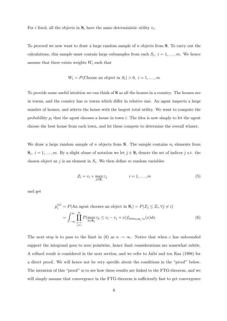
For i fixed, all the objects in Si have the same deterministic utility vi.

To proceed we now want to draw a large random sample of n objects from S. To carry out the

calculations, this sample must contain large subsamples from each Si, i = 1, . . . ,m. We hence

assume that there exists weights Wi such that

Wi = P (Choose an object in Si) > 0, i = 1, . . . ,m

To provide some useful intuition we can think of S as all the houses in a country. The houses are

in towns, and the country has m towns which differ in relative size. An agent inspects a large

number of houses, and selects the house with the largest total utility. We want to compute the

probability pi that the agent chooses a house in town i. The idea is now simply to let the agent

choose the best house from each town, and let these compete to determine the overall winner.

We draw a large random sample of n objects from S. The sample contains ni elements from

Si, i = 1, . . . ,m. By a slight abuse of notation we let j ∈ Si denote the set of indices j s.t. the

chosen object nr j is an element in Si. We then define m random variables

Zi = vi + maxj∈Si

εj i = 1, . . . ,m (5)

and get

p(n)i = P (An agent chooses an object in Si) = P (Zj ≤ Zi,∀j 6= i)

=∫ ∞−∞

m∏j=1j 6=i

P (maxk∈Sj

εk ≤ vi − vj + x)fmaxk∈Siεk

(x)dx (6)

The next step is to pass to the limit in (6) as n → ∞. Notice that when ε has unbounded

support the integrand goes to zero pointwise, hence limit considerations are somewhat subtle.

A refined result is considered in the next section, and we refer to Jaibi and ten Raa (1998) for

a direct proof. We will hence not be very specific about the conditions in the “proof” below.

The intention of this “proof” is to see how these results are linked to the FTG-theorem, and we

will simply assume that convergence in the FTG-theorem is sufficiently fast to get convergence

6

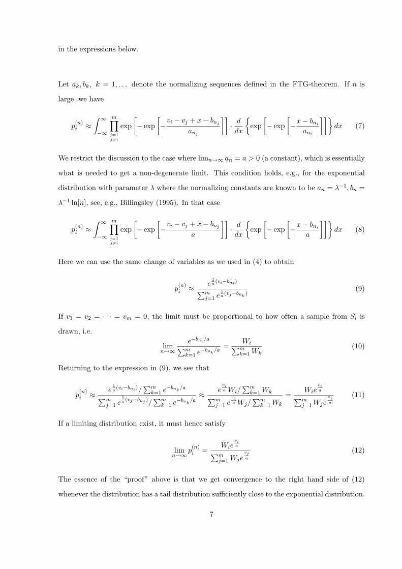
in the expressions below.

Let ak, bk, k = 1, . . . denote the normalizing sequences defined in the FTG-theorem. If n is

large, we have

p(n)i ≈

∫ ∞−∞

m∏j=1j 6=i

exp[− exp

[−vi − vj + x− bnj

anj

]]· ddx

{exp

[− exp

[−x− bni

ani

]]}dx (7)

We restrict the discussion to the case where limn→∞ an = a > 0 (a constant), which is essentially

what is needed to get a non-degenerate limit. This condition holds, e.g., for the exponential

distribution with parameter λ where the normalizing constants are known to be an = λ−1, bn =

λ−1 ln[n], see, e.g., Billingsley (1995). In that case

p(n)i ≈

∫ ∞−∞

m∏j=1j 6=i

exp[− exp

[−vi − vj + x− bnj

a

]]· ddx

{exp

[− exp

[−x− bni

a

]]}dx (8)

Here we can use the same change of variables as we used in (4) to obtain

p(n)i ≈ e

1a(vi−bni )∑m

j=1 e1a(vj−bnk

)(9)

If v1 = v2 = · · · = vm = 0, the limit must be proportional to how often a sample from Si is

drawn, i.e.

limn→∞

e−bni/a∑mk=1 e

−bnk/a

=Wi∑mk=1Wk

(10)

Returning to the expression in (9), we see that

p(n)i ≈

e1a(vi−bni )/

∑mk=1 e

−bnk/a∑m

j=1 e1a(vj−bnj )/

∑mk=1 e

−bnk/a≈

evia Wi/

∑mk=1Wk∑m

j=1 evja Wj/

∑mk=1Wk

=Wie

via∑m

j=1Wjevja

(11)

If a limiting distribution exist, it must hence satisfy

limn→∞

p(n)i =

Wievia∑m

j=1Wjevja

(12)

The essence of the “proof” above is that we get convergence to the right hand side of (12)

whenever the distribution has a tail distribution sufficiently close to the exponential distribution.

7

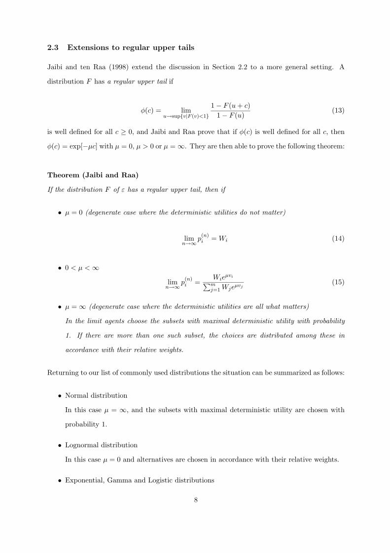
2.3 Extensions to regular upper tails

Jaibi and ten Raa (1998) extend the discussion in Section 2.2 to a more general setting. A

distribution F has a regular upper tail if

φ(c) = limu→sup{v|F (v)<1}

1− F (u+ c)1− F (u)

(13)

is well defined for all c ≥ 0, and Jaibi and Raa prove that if φ(c) is well defined for all c, then

φ(c) = exp[−µc] with µ = 0, µ > 0 or µ =∞. They are then able to prove the following theorem:

Theorem (Jaibi and Raa)

If the distribution F of ε has a regular upper tail, then if

• µ = 0 (degenerate case where the deterministic utilities do not matter)

limn→∞

p(n)i = Wi (14)

• 0 < µ <∞

limn→∞

p(n)i =

Wieµvi∑m

j=1Wjeµvj(15)

• µ =∞ (degenerate case where the deterministic utilities are all what matters)

In the limit agents choose the subsets with maximal deterministic utility with probability

1. If there are more than one such subset, the choices are distributed among these in

accordance with their relative weights.

Returning to our list of commonly used distributions the situation can be summarized as follows:

• Normal distribution

In this case µ = ∞, and the subsets with maximal deterministic utility are chosen with

probability 1.

• Lognormal distribution

In this case µ = 0 and alternatives are chosen in accordance with their relative weights.

• Exponential, Gamma and Logistic distributions

8

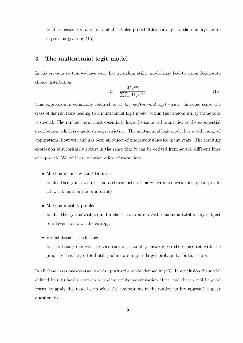
In these cases 0 < µ < ∞, and the choice probabilities converge to the non-degenerate

expression given by (15).

3 The multinomial logit model

In the previous section we have seen that a random utility model may lead to a non-degenerate

choice distribution

pi =Wie

µvi∑mj=1Wjeµvj

(16)

This expression is commonly referred to as the multinomial logit model. In some sense the

class of distributions leading to a multinomial logit model within the random utility framework

is special. The random term must essentially have the same tail properties as the exponential

distribution, which is a quite strong restriction. The multinomial logit model has a wide range of

applications, however, and has been an object of intensive studies for many years. The resulting

expression is surprisingly robust in the sense that it can be derived from several different lines

of approach. We will here mention a few of these lines.

• Maximum entropy considerations

In this theory one wish to find a choice distribution which maximizes entropy subject to

a lower bound on the total utility.

• Maximum utility problem

In this theory one wish to find a choice distribution with maximum total utility subject

to a lower bound on the entropy.

• Probabilistic cost efficiency

In this theory one wish to construct a probability measure on the choice set with the

property that larger total utility of a state implies larger probability for that state.

In all these cases one eventually ends up with the model defined in (16). In conclusion the model

defined by (16) hardly rests on a random utility maximization alone, and there could be good

reason to apply this model even when the assumptions in the random utility approach appear

questionable.

9

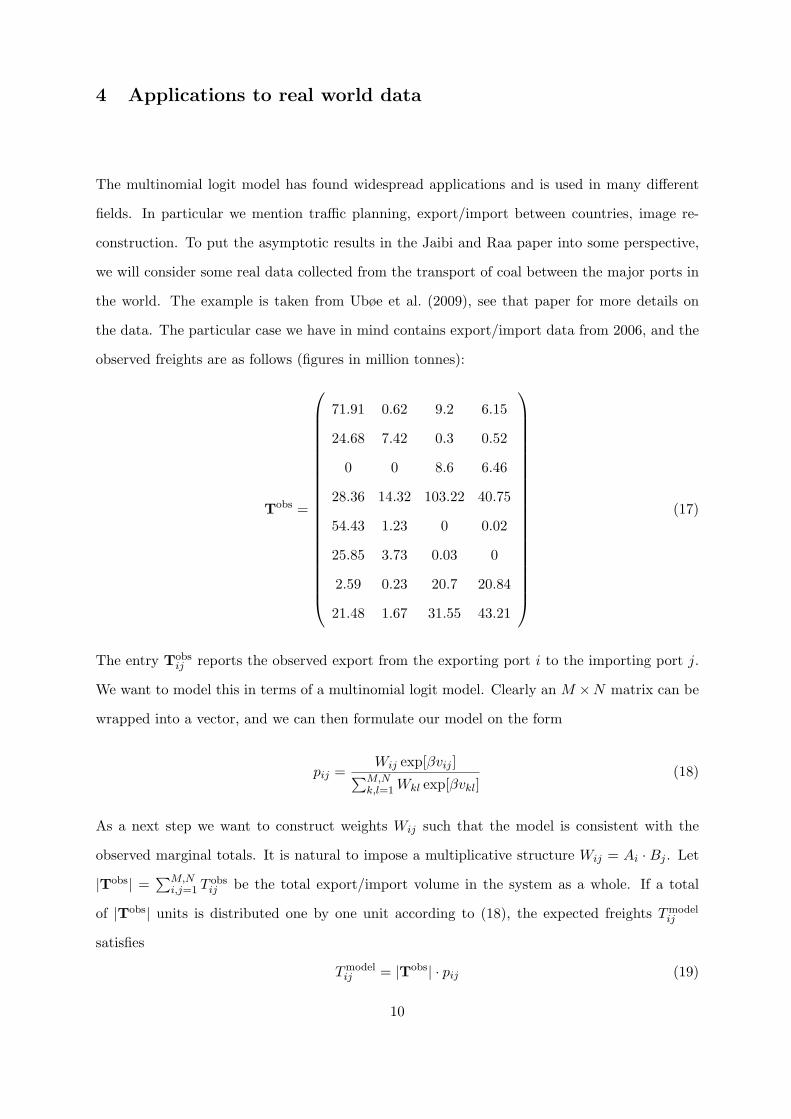
4 Applications to real world data

The multinomial logit model has found widespread applications and is used in many different

fields. In particular we mention traffic planning, export/import between countries, image re-

construction. To put the asymptotic results in the Jaibi and Raa paper into some perspective,

we will consider some real data collected from the transport of coal between the major ports in

the world. The example is taken from Ubøe et al. (2009), see that paper for more details on

the data. The particular case we have in mind contains export/import data from 2006, and the

observed freights are as follows (figures in million tonnes):

Tobs =

71.91 0.62 9.2 6.15

24.68 7.42 0.3 0.52

0 0 8.6 6.46

28.36 14.32 103.22 40.75

54.43 1.23 0 0.02

25.85 3.73 0.03 0

2.59 0.23 20.7 20.84

21.48 1.67 31.55 43.21

(17)

The entry Tobsij reports the observed export from the exporting port i to the importing port j.

We want to model this in terms of a multinomial logit model. Clearly an M ×N matrix can be

wrapped into a vector, and we can then formulate our model on the form

pij =Wij exp[βvij ]∑M,N

k,l=1Wkl exp[βvkl](18)

As a next step we want to construct weights Wij such that the model is consistent with the

observed marginal totals. It is natural to impose a multiplicative structure Wij = Ai · Bj . Let

|Tobs| =∑M,N

i,j=1 Tobsij be the total export/import volume in the system as a whole. If a total

of |Tobs| units is distributed one by one unit according to (18), the expected freights Tmodelij

satisfies

Tmodelij = |Tobs| · pij (19)

10

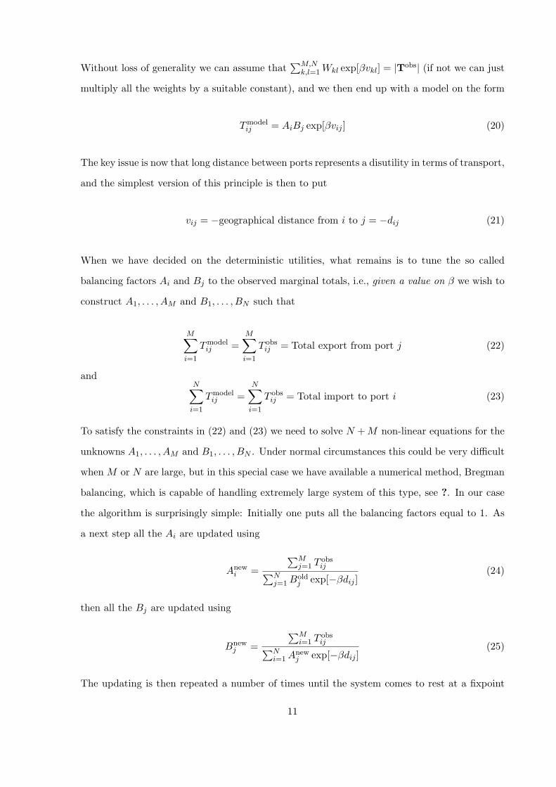
Without loss of generality we can assume that∑M,N

k,l=1Wkl exp[βvkl] = |Tobs| (if not we can just

multiply all the weights by a suitable constant), and we then end up with a model on the form

Tmodelij = AiBj exp[βvij ] (20)

The key issue is now that long distance between ports represents a disutility in terms of transport,

and the simplest version of this principle is then to put

vij = −geographical distance from i to j = −dij (21)

When we have decided on the deterministic utilities, what remains is to tune the so called

balancing factors Ai and Bj to the observed marginal totals, i.e., given a value on β we wish to

construct A1, . . . , AM and B1, . . . , BN such that

M∑i=1

Tmodelij =

M∑i=1

T obsij = Total export from port j (22)

andN∑i=1

Tmodelij =

N∑i=1

T obsij = Total import to port i (23)

To satisfy the constraints in (22) and (23) we need to solve N +M non-linear equations for the

unknowns A1, . . . , AM and B1, . . . , BN . Under normal circumstances this could be very difficult

when M or N are large, but in this special case we have available a numerical method, Bregman

balancing, which is capable of handling extremely large system of this type, see ?. In our case

the algorithm is surprisingly simple: Initially one puts all the balancing factors equal to 1. As

a next step all the Ai are updated using

Anewi =

∑Mj=1 T

obsij∑N

j=1Boldj exp[−βdij ]

(24)

then all the Bj are updated using

Bnewj =

∑Mi=1 T

obsij∑N

i=1Anewj exp[−βdij ]

(25)

The updating is then repeated a number of times until the system comes to rest at a fixpoint

11

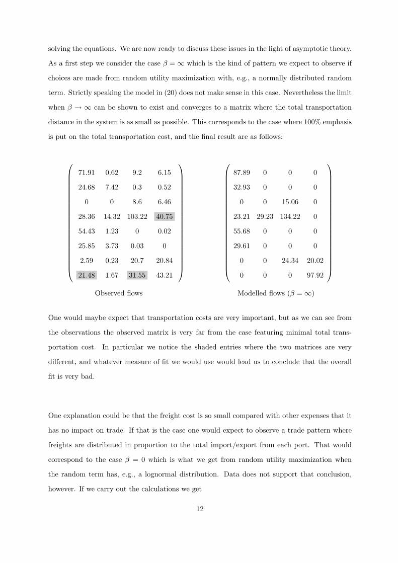
solving the equations. We are now ready to discuss these issues in the light of asymptotic theory.

As a first step we consider the case β =∞ which is the kind of pattern we expect to observe if

choices are made from random utility maximization with, e.g., a normally distributed random

term. Strictly speaking the model in (20) does not make sense in this case. Nevertheless the limit

when β → ∞ can be shown to exist and converges to a matrix where the total transportation

distance in the system is as small as possible. This corresponds to the case where 100% emphasis

is put on the total transportation cost, and the final result are as follows:

71.91 0.62 9.2 6.15

24.68 7.42 0.3 0.52

0 0 8.6 6.46

28.36 14.32 103.22 40.75

54.43 1.23 0 0.02

25.85 3.73 0.03 0

2.59 0.23 20.7 20.84

21.48 1.67 31.55 43.21

87.89 0 0 0

32.93 0 0 0

0 0 15.06 0

23.21 29.23 134.22 0

55.68 0 0 0

29.61 0 0 0

0 0 24.34 20.02

0 0 0 97.92

Observed flows Modelled flows (β =∞)

One would maybe expect that transportation costs are very important, but as we can see from

the observations the observed matrix is very far from the case featuring minimal total trans-

portation cost. In particular we notice the shaded entries where the two matrices are very

different, and whatever measure of fit we would use would lead us to conclude that the overall

fit is very bad.

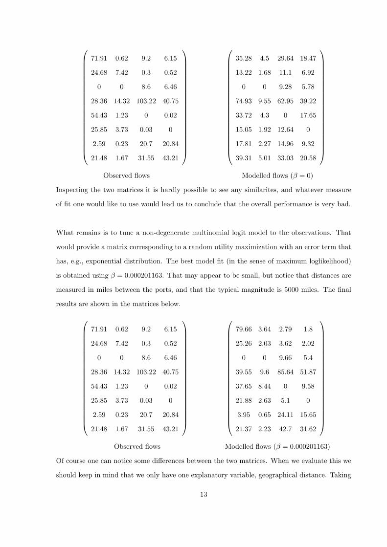
One explanation could be that the freight cost is so small compared with other expenses that it

has no impact on trade. If that is the case one would expect to observe a trade pattern where

freights are distributed in proportion to the total import/export from each port. That would

correspond to the case β = 0 which is what we get from random utility maximization when

the random term has, e.g., a lognormal distribution. Data does not support that conclusion,

however. If we carry out the calculations we get

12

71.91 0.62 9.2 6.15

24.68 7.42 0.3 0.52

0 0 8.6 6.46

28.36 14.32 103.22 40.75

54.43 1.23 0 0.02

25.85 3.73 0.03 0

2.59 0.23 20.7 20.84

21.48 1.67 31.55 43.21

35.28 4.5 29.64 18.47

13.22 1.68 11.1 6.92

0 0 9.28 5.78

74.93 9.55 62.95 39.22

33.72 4.3 0 17.65

15.05 1.92 12.64 0

17.81 2.27 14.96 9.32

39.31 5.01 33.03 20.58

Observed flows Modelled flows (β = 0)

Inspecting the two matrices it is hardly possible to see any similarites, and whatever measure

of fit one would like to use would lead us to conclude that the overall performance is very bad.

What remains is to tune a non-degenerate multinomial logit model to the observations. That

would provide a matrix corresponding to a random utility maximization with an error term that

has, e.g., exponential distribution. The best model fit (in the sense of maximum loglikelihood)

is obtained using β = 0.000201163. That may appear to be small, but notice that distances are

measured in miles between the ports, and that the typical magnitude is 5000 miles. The final

results are shown in the matrices below.

71.91 0.62 9.2 6.15

24.68 7.42 0.3 0.52

0 0 8.6 6.46

28.36 14.32 103.22 40.75

54.43 1.23 0 0.02

25.85 3.73 0.03 0

2.59 0.23 20.7 20.84

21.48 1.67 31.55 43.21

79.66 3.64 2.79 1.8

25.26 2.03 3.62 2.02

0 0 9.66 5.4

39.55 9.6 85.64 51.87

37.65 8.44 0 9.58

21.88 2.63 5.1 0

3.95 0.65 24.11 15.65

21.37 2.23 42.7 31.62

Observed flows Modelled flows (β = 0.000201163)

Of course one can notice some differences between the two matrices. When we evaluate this we

should keep in mind that we only have one explanatory variable, geographical distance. Taking

13

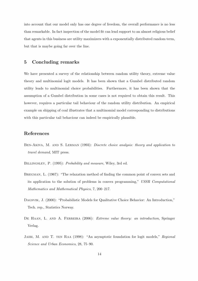
into account that our model only has one degree of freedom, the overall performance is no less

than remarkable. In fact inspection of the model fit can lend support to an almost religious belief

that agents in this business are utility maximizers with a exponentially distributed random term,

but that is maybe going far over the line.

5 Concluding remarks

We have presented a survey of the relationship between random utility theory, extreme value

theory and multinomial logit models. It has been shown that a Gumbel distributed random

utility leads to multinomial choice probabilities. Furthermore, it has been shown that the

assumption of a Gumbel distribution in some cases is not required to obtain this result. This

however, requires a particular tail behaviour of the random utility distribution. An empirical

example on shipping of coal illustrates that a multinomial model corresponding to distributions

with this particular tail behaviour can indeed be empirically plausible.

References

Ben-Akiva, M. and S. Lerman (1993): Discrete choice analysis: theory and application to

travel demand, MIT press.

Billingsley, P. (1995): Probability and measure, Wiley, 3rd ed.

Bregman, L. (1967): “The relaxation method of finding the common point of convex sets and

its application to the solution of problems in convex programming,” USSR Computational

Mathematics and Mathematical Physics, 7, 200–217.

Dagsvik, J. (2000): “Probabilistic Models for Qualitative Choice Behavior: An Introduction,”

Tech. rep., Statistics Norway.

De Haan, L. and A. Ferreira (2006): Extreme value theory: an introduction, Springer

Verlag.

Jaibi, M. and T. ten Raa (1998): “An asymptotic foundation for logit models,” Regional

Science and Urban Economics, 28, 75–90.

14

Leonardi, G. (1984): “The structure of random utility models in the light of the asymptotic

theory of extremes,” in Transportation Planning Models, ed. by M. Florian, 107–133.

Manski, C. (1977): “The structure of random utility models,” Theory and decision, 8, 229–254.

McFadden, D. (1972): Conditional logit analysis of qualitative choice behaviour, Univ of Cali-

fornia, Instit of Urban and Regional Development.

McFadden, D. et al. (1978): “Modelling the choice of residential location,” Spatial interaction

theory and planning models, 25, 75–96.

Ubøe, J., J. Andersson, K. Jornsten, and S. Strandenes (2009): “Modeling freight

markets for coal,” Maritime Economics and Logistics, 11, 289–301.

15