SOME ADVANCES IN THE ANALYSIS OF FLUID …web.mit.edu/.../Some_advances_in_the_analysis_of_fluid_flows.pdfSOME ADVANCES IN THE ANALYSIS OF FLUID FLOWS? ... be regarded as a report

Pergamon

Compuars & Slructures Vol. 64, No. 5/6, pp. 909-930, 1997

0 1997 Elsevier Science Ltd. All rights reserved

PII: soo45-7949(97)ooo4o-o Printed in Gnat Britain

004s7949197 117.00 + 0.00

SOME ADVANCES IN THE ANALYSIS OF FLUID FLOWS?

K. J. Bathex, H. Zhangg and X. Zhangt

iMassachusetts Institute of Technology, Cambridge, MA 02139, U.S.A. $ADINA R & D, Inc., Watertown, MA 02172, U.S.A.

Abstract-We review some new solution capabilities developed and available in the ADINA-F CFD (computational fluid dynamics) program and present example solutions. Unique features and advances are that incompressible and compressible flows with structural interactions can be analyzed and that a general radiation heat transfer analysis capability based on specular and diffusive reflectivities and transmittance is available. This paper is largely a continuation of the presentation given in Ref. [I]. 0 1997 Elsevier Science Ltd.

1. INTRODUCTION

The solution of fluid flows has, during recent years, attracted great interest, largely because available computer hardware and software now make it possible to solve, realistically, three-dimensional fluid flows on engineering workstations. We have developed the ADINA-F CFD program for the analysis of fluid flows. As presented in Ref. [l], some unique features of the program are that it can be used to analyze incompressible flows (with or without heat transfer), compressible flows, free-surface flows and the analysis of these flow conditions with the full interaction of structures modeled with the capabilities of ADINA.

Our objective in this paper is to present the developments in ADINA-F that we have undertaken during the last two years (that is, since the writing of Ref. [l]), and show some example solutions. While, in essence, this paper can be thought of as a continuation of Ref. [l], the paper is, nevertheless, a self-contained presentation.

In Section 2, we review the governing fluid-flow equations and remark upon solution strategies. The solution procedures are of interest because incompressible and compressible flows can be analyzed and an arbitrary Lagrangian-Eulerian formulation is employed when structural interactions are included.

In Section 3, we then present a new radiation analysis capability that includes specular and diffusive reflectivities and transmittance. Ray tracing over the actual geometry is employed and thus no view factors are input when using the analysis capability. This analysis feature is very useful and has found applications, for example, in the simu- lation of fluid flows and heat transfer in motor-car headlamps. We finally present various example solutions obtained with ADINA-F in Section 4.

tSome of the original figures for this paper were generated with a color-producing terminal and submitted in color.

These solutions include fluid flows with structural interactions and show some unique features of the program.

Of course, we are continuing our development in the CFD area, and on ADINA-F, including structural interactions. Hence, this paper should only be regarded as a report on the current status of our work. In the conclusions of the paper, we briefly point toward our future developments in the field. These developments promise to be most exciting indeed because of the many physical phenomena that, eventually, we want to simulate in fluid flows with structural interactions.

2. FLUID-FLOW EQUATIONS

In this section, we briefly summarize the fluid-flow equations that we can solve with ADINA-F. The presentation defines the mathematical models that can be assumed for the fluid flow and gives the solution strategies that are available. As previously mentioned, we consider incompressible and compressible flows, including structural interactions.

2.1. Incompressible fluid-flow equations

We assume a Navier-Stokes fluid described in a stationary Cartesian coordinate system (xi, i = 1,2,3) [l, 21. The fluid-flow equations governing incompressible flows, with heat transfer are in conservative form:

g + V(F - G) = S (1)

with

(2)

(3)

CAS 64/S-&B 909

910 K. J. Bathe

Table 1. Possible boundary conditions directly available for compressible flow analysis using ADINA-F

Type of boundary Variable combinations

External (p. C, M) or (0, P, ~1) Inlet-subsonic (p. H), (p, 0). (0, L.), (0,pr). (p. 1.). or (H. r>) Outlet-subsonic p, 0, p. or c Inlet-supersonic (p. I‘, M), (p. 0, c.), or (P, L’. M) Outlet-supersonic (no variables required) Wall n Symmetry (no variables required) Flu&structure interaction 0 Free surface P

where p = density. 0 = temperature, M = Mach number, H = enthalpy, p = pressure, e = internal energy, 2‘ = velocity.

G= y I I -q (4)

0 s= F I I f% + q8

(5)

where v is the velocity vector; p is the mass density; E is the specific energy = l/2 WV + e; e is the internal energy; r is the stress tensor; q is the vector of heat flows; f* is the vector of externally applied body forces (which can include the forces due to rotations that the fluid is subjected to); and qB is the rate of heat generated per unit volume.

The components of the stress tensor t are given by:

gray transparent surface

c, = -P&, + be,, (6)

where p is the pressure, 6,, is the Kronecker delta, p is the viscosity, and the components of the velocity

strain tensor e are given by

(7)

The components of the heat flow vector q are given

by:

q, = -kB,, (8)

where k is the thermal conductivity and 8 is the temperature. The internal energy, e, is given by de = c, d0, and c, = cP where c, and cp are the specific

heats at constant volume and constant pressure, respectively.

incident unit of

diffusely rellected energy

specldarly reflected

absorbed energy

y transmitted energy (lost to environment)

Fig. 1. Schematic representation of radiation energies corresponding to an incident ray.

Advances in analysis of fluid flows 911

Fig. 2. Concrete tank being filled with oil (half tank and fluids are shown and modeled).

The boundary conditions for the solution of eqn (1) comprise prescribed velocities and tractions for the momentum equations, and prescribed temperatures, prescribed heat fluxes, convection and/or radiation conditions for the energy equation. A useful capability is that the prescribed boundary condition values can be associated with a ‘birth’ and ‘death option. This means that a prescribed boundary value can be inactive until its time of birth and can become inactive at its time of death.

In eqn (l), the material descriptions can be constant, temperature- or time-dependent. The laminar viscosity can also be modeled using power laws or the Carreau model. The Boussinesq approximation is used for modeling the buoyancy force.

Equation (1) governs the laminar flow conditions. To model turbulence, the mixing-length model (for which the user has to program the mixing-length definition), the standard Kt, the RNG K-e models and the K-U models for high and low Reynolds number flows can be used. Of course, using the K-c or K-W models, additional equations need to be solved for K, 6 or w, whichever are applicable [3,4].

Finally, we should mention that incompressible fluid flow through porous media can also be analyzed based on the solution of the following equations:

$= -P.+Pg,[l -B(B-8,)] (9)

ui,i = 0 (10)

pz,; + q5 pc, vi e,i = ( >

Le,, ,i + qB (11)

and

(12)

k’ = f#& + (1 - 4)/c, (13)

where 4 is the porosity; Q is the permeability in the x,-direction; g, is the component of gravity in the x,-direction; /_I is the coefficient of volume expansion; and 0, is the reference temperature in the Boussinesq assumption of buoyancy; the subscript ‘s’ refers to the solid phase. As usual, the boundary conditions consist of prescribed velocities, pressure, temperature and heat fluxes [l].

2.2. Compressible fluid-flow equations

The Navier-Stolces equations governing compressible fluid flows are:

g +V. F-G =S ( >

where, now,

(1%

PV F= pw+pI

[ 1 PVH

(16)

912 K. J. Bathe

1

Advances in analysis of fluid flows

VELOCITY

0.001625

0.001375

0.001125

0.000675

omO625

0.000375

0.000125

52.50

46.50

36.50

31.50

24.50

17.50

10.50

Fig. 4. Velocity field and temperature distribution viewed from the back of the tank at (almost) the middle of oil injection.

(17)

P = P(P@)

e = 4P,@

(19)

(20)

and S was already defined in eqn (5). Here the components of the stress tensor ; are

which for a perfect gas give p = p/((c, - c,)Q) and = c,B. In ADINA-F, the general form

i,, = h,,d,, + 2pe,, (18)

with I as the second viscosity (in Stokes’ hypothesis 1= - ; p) and H is the enthalpy ( = E + p/p). We note that by neglecting all diffusive and viscous effects (that is, by setting G = 0 in eqn (14)), we obtain the Euler equations. With ADINA-F we can solve the full Navier-Stokes eqns (14) - (17) or the Euler equations.

To close the governing equation system for the compressible fluid flow, the equations of state must be included:

of eqns (19) and (20) can be used, or the assumption of a perfect gas can be made. Therefore, eqns (14t( 17) must always be solved considering temperature effects, whereas the incompressible flow

equations can be solved with or without the energy equation.

Of course, the solution of eqns (14) - (20) requires the appropriate specification of boundary conditions. The number of boundary variables that must be specified depends on the type of flow. With ADINA-F, external and internal, subsonic, transonic and supersonic flows can be solved and various

914 K. J. Bathe

combinations of variables can be employed to specify the boundary conditions. Table 1 summarizes the possible specifications. This choice gives the user some ease and flexibility to specify the boundary conditions according to the theoretical or measured data at hand. We note that these boundary conditions are given in terms of primitive and additional variables. However, in the program solution, the conservative variables listed in U in eqn (15) are always employed. Hence, these variables can also directly be prescribed.

The material parameters are assumed to be either constant, temperature-dependent, pressure-dependent or temperature and pressure-dependent. Except for the constant case, the laminar viscosity p and the conductivity k are defined by the Sutherland formulas:

P = P@)‘(~)

k = k,(;)‘.(@j

(21)

(22)

where pO and k, are the viscosity at the reference temperature 0, and conductivity at the reference temperature O,, respectively, m, and m, are constants and S, and S, are selected constant temperature values. To model turbulence effects, the standard compressible K--t model can be employed [3,4].

2.3. Arbitrary Lagrangian-Eulerian formulation

To analyze free-surface flows and the interactions of flows with structures, we use an arbitrary Lagrangian-Eulerian (ALE) formulation of the governing fluid-flow equations given above. Let us

first summarize the various flow conditions that require this formulation.

2.3.1. Free surface. The kinematic boundary condition of a free surface S(xi, t) is:

g + visti = 0

and the dynamic boundary condition is

T&=[-Po+u(~ •k &)]n, (24)

where pO is the externally applied pressure on the surface; u is the surface tension; n, denotes the components of the unit vector normal to the free surface and R, and R2 denote the radii of curvatures of the free surface. The motion of the free surface requires, in ADINA-F, that the mesh be moved during the solution (the mesh shall always bound the fluid region), and this necessitates the use of the ALE formulation.

2.3.2. Interface between two fluid media. We consider two fluid media that are immiscible. The kinematic boundary condition is as in eqn (23) and the dynamic boundary condition is now:

Qn, - $?‘n, = --Q n, (25)

where all variables are as in eqn (24) and rv) and rf) denote the stress components of the two fluids at the interface. The ALE formulation is used for the same reason as in free-surface calculations.

2.3.3. Moving wall. Considering a moving solid boundary, the kinematic interface conditions are:

VP = a(‘) (26)

Fig. 5. Turbulent jet entering channel.


ADINA-F

(4

z -4 Y

VELOCITY TIME 36.05

1 6.062

5.600 4.600

4.000

3.200

2.400

1.600 0.600

_ Fig, 6. (a) Velocity distribution for jet entering channel; (b) pressure and velocity distributions for jet near

entrance.

916 K. J. Bathe

dV’ = d’“’ / I (27)

where d, denotes the components of the displacements and the superscripts (s) and (f) refer to the solid and fluid particles at the interface.

The dynamic boundary condition is:

T;’ = Tj;’ (28)

Equations (26) - (28) assume the no-slip condition of the fluid on the wall. A slip condition can also be imposed, in which case the tangential velocities of the fluid particles on the interface are free, that is, they are not constrained by the wall. This condition is applicable when the fluid is modeled by the Euler equations. The boundary conditions of a moving wall are applicable if the movement of a rigid wall boundary is prescribed by the analyst for the ADINA-F solution or if the motion of a flexible solid boundary as calculated using ADINA is prescribed for the ADINA-F solution. Since the fluid domain changes in these solutions, the ALE formulation is used.

2.3.4. Fluid-structure interactions. Using the ADINA System, the full coupling of incompressible or compressible fluid flows with structural motions can be analyzed. The structure can be modeled with ail the analysis features available in the structural finite element program ADINA. The coupling is achieved using the wall interface conditions described above and iterating between the programs ADINA and ADINA-F to obtain a sufficiently converged solution in each time step. The staggered solution process is automatic and can be employed for transient and steady-state analyses. Of course, the

ALE formulation is used for the fluid flow because the fluid domain changes during the analysis process.

We may note that all the above boundary conditions can, of course, be used in a single analysis (provided these conditions represent, in their combined form, physically realistic conditions).

2.3.5. ALE method. The main characteristic of the boundary conditions described in this section is that the fluid domain changes during the solution. This change in the fluid domain is either imposed onto the ADINA-F solution by a wall or fluid-structure boundary, or is calculated as for the free surface or interface between two different fluids. This characteristic is dealt with in the ALE method by allowing the finite element mesh of the fluid to move. The mesh movement on the moving boundaries is prescribed to follow the physical conditions but is automatically adjusted tangentially to preserve a reasonable mesh quality. For the same reason, nodes inside the fluid domain are also adjusted in their positions, of course, without local constraints of movement. The new nodal positions are calculated by solving first the Laplace equation for the boundary lines, then for the surfaces and finally for the volumes used in modeling the fluid domain. Each time, the available (and just calculated) information is used as boundary conditions for the next Laplace equation problem to obtain improved nodal positions.

The movement in the nodal positions resulting in the mesh velocity v, then enters the calculation of the

hpemeable rock

Fig. 7. Cross-section of the dam and surrounding. 0, = 4°C 0. = - 2O”C, tip = IOOC, H, = 25 m, Hd = 5 m.


(4 ADINA-F

99.0

61.0

63.0

45.0

27.0

9.0

-9.0

0.02526

‘< ‘, .j _;

0.02275 0.01925 0.01575 0.01225 0.00675 -...-.-. j, :: -“-t. ~;““‘“z...________. 0.00525

” ._ ._ _ . .._-- . . _. _ -_.e-------.li 0.00175

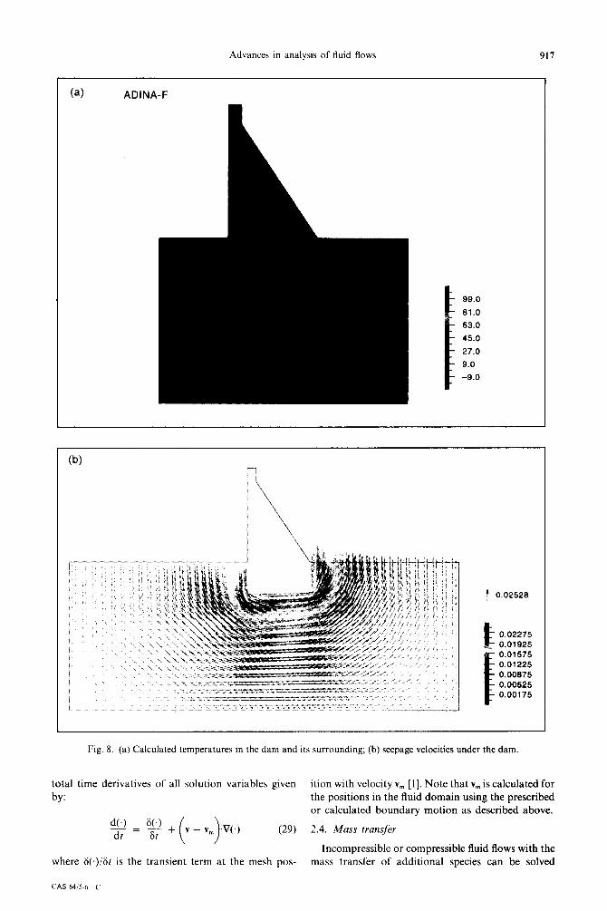
Fig. 8. (a) Calculated temperatures in the dam and its surrounding: (b) seepage velocities under the dam.

total time derivatives of all solution variables given ition with velocity v, [l]. Note that v, is calculated for by: the positions in the fluid domain using the prescribed

or calculated boundarv motion as described above.

dC.1 _=- dt

. (29) 2.4. Mass transfer

\ I

Incompressible or compressible fluid flows with the where 6(.)/6t is the transient term at the mesh pos- mass transfer of additional species can be solved

CAS 64~5.6 C

918 K. J. Bathe

using ADINA-F. The governing fluid-flow equations are then those presented in Sections 2.1 and 2.2 plus the following mass transfer equations for i = I,..., N:

a(pdd at + pmv,wI - &,w,,, > ,, = m, (30)

where N is the number of additional species, pt is the density of the ith species,

Pm = P + i PI, ,=I

p is the fluid density,

w, = P,lPm

is the mass ratio of the ith species, mi is the mass creation rate of the ith species and the D, are the components of the diffusivity tensor. The diffusivity coefficients can be assumed to be either constant, dependent on the velocity and flow directions, or pressure and temperature dependent [3].

The boundary conditions include prescribed mass ratios, mass fluxes and mass convections of each species.

2.5. Finite element solution

The finite element discretization of the governing fluid-flow equations is obtained as described in Ref. [2]. For two-dimensional solutions, the three-

i

Fig. 9. Flow device.

node triangular element is used, and for three- dimensional solutions, the four-node tetrahedral element is used. Both elements satisfy the inf-sup condition because they have a bubble interpolation for the velocities [2]. The elements are referred to in Ref. [2] as the 4/3-c and 5/4-c elements, respectively (for the two-dimensional element, the ‘4’ refers to the three corner nodes velocity interpolation plus the bubble function for the velocity, the ‘3’ refers to the three comer nodes pressure interpolation and the ‘c’ refers to the fact that the pressure between elements is continuous; similarly, for the tetrahedral element).

In addition to these elements, a 9-node and a 27-node element can be used, respectively, for two-dimensional and three-dimensional low Reynolds and Peclet number incompressible flows.

The use of the triangular and tetrahedral elements is attractive for free-meshing of arbitrary geometries. This feature is available in the ADINA-IN pre-pro- cessor for the ADINA-F program in the ADINA System and, in particular, can be employed with Pro/ENGINEER by directly operating on the Pro/E geometry. Problems modeled with I-DEAS and PATRAN can also be solved directly with the ADINA-F program through the use of the translator program TRANSOR for pre- and post-processing.

An important feature for fluid-structure interaction analysis is that the mesh for the fluid can be generated entirely independently from the generation of the mesh for the structure. Indeed, usually a relatively fine mesh must be used for the fluid compared to the mesh employed for the structure. During the analysis, the solution algorithm ensures that the fluid nodes remain on the structural surfaces.

The assembled equations are solved in steady-state analysis using a GMRES or biconjugate gradient iterative scheme with incomplete Cholesky pre-con- ditioning. The same procedures are also used in transient analysis using implicit integration with the Euler method [2]. Full explicit integration using theEuler forward method can be employed for compressible flow solutions, whereas in incompressible flow analysis, only the momentum and energy equations can be solved explicitly while the continuity equation is always solved implicitly.

3. SPECULAR-DIFFUSIVE RADIATION

A special feature offered in ADINA-F is that specular-diffusive radiation conditions can be analyzed. Figure 1 shows a portion of a surface surrounding a fluid and, schematically, the assumptions used.

The surface is assumed to be gray, transparent and diffusely and specularly reflective [5]. Consider an incident unit ray of energy. This ray is decomposed into four portions:

l a diffusely reflected portion (d); l a transmitted portion (t);

Advances in analysis of fluid Rows 919

r

920 K. J. Bathe

l an absorbed portion (a), where by Kirchhoh’s law a = e; e is the emittance;

l a specularly reflected portion (s).

The coefficients s, d, t can be constants or can depend on either a component of velocity, the pressure or the temperature. They are prescribed by the user and the coefficient 2 is calculated by the program using:

a+s+d+t=l. (31)

The transmitted energy is lost to the environment and not traced in the solution and the diffusely reflected energy is accounted for using Lambert’s law. In addition, the specularly reflected energy is calculated in the solution algorithm by tracing the reflected ray of energy using that a, = LY,, see Fig. 1.

The objective of the analysis is to calculate the heat flux into the fluid and, if applicable, to the surrounding solid due to the conditions on the radiating surfaces. The governing equations are established using radiosity as an additional degree of freedom on the radiation surfaces.

Defining RI to be the rate of outgoing radiant energy per unit area at the material point k, we have

Rt = e,o,t% + 4G, + tkfkot0,4 (32)

where G is the rate of incoming radiant energy per unit area, .f is the shape factor (from the environment), 8, is the environmental temperature. CT is the Stefan-Boltzmann constant and the subscript I\- refers to the material point k.

The rate of energy leaving the specular boundaries and arriving at the material point is giving GA:

G, = RIF;mldA, (33)

where. in the calculation of F; i, a unit area at point ic is considered and the integration is performed over all radiating surfaces (denoted as A,). The view factor F; i is calculated using a ray tracing technique

based on Lambert’s law. The finite element solution of eqn (32) is obtained

by allocating the radiosity degree of freedom at the finite element nodes on the radiation surfaces. Hence, we have:

R = zh,R,

where we sum over all element nodes that affect the value of R at the point considered.

Substituting from eqns (33) and (34) into eqn (32) and using the Galerkin method for node i, we

obtain [2]:

[ j?h.d+, - [j; h,( ~V”dA)da]R, (35)

I

I I

I

I I

,I,-________ //-f --# fl _&__-____A---- --

.’ . ,:;jy ,I--

piston

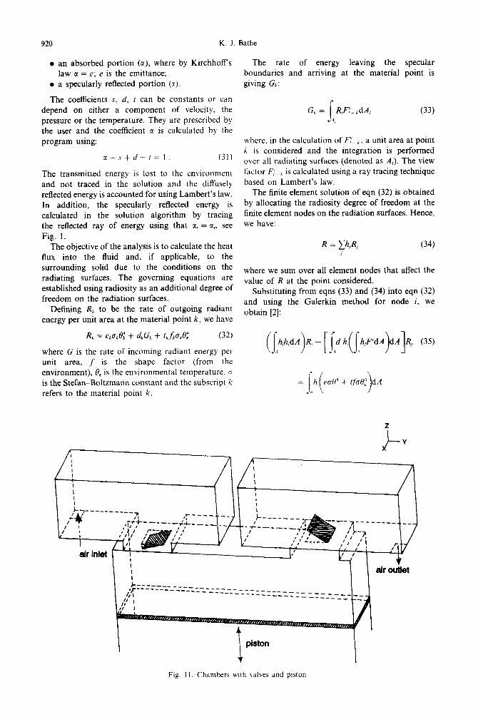
Fig. I I. Chambers with valves and piston.

I airouiet


922 K. J. Bathe


F si %g. 14. Flow near right valve: (a) just before opening (b) just after opening [one time step after t ituation]; (c) valve is fully open; (d) valve starts closing; (e) valve is almost closed; (f) valve is close

time step after the (e) situation]. (Continued overleaf.)

:he (a) d [I 3ne

924 K. J. Bathe


Fig. 14(e)--Continued.

926 K. J

where hi denotes the interpolation function and A corresponds to all element surface areas that take part in the radiation process. Note that F is defined in eqn (33), where it is understood that in eqn (39, the F depends on the material points considered in the double integrations.

Having solved eqn (35) for the nodal radiosities, we calculate the heat flux generated at the radiation surface as the difference of the absorbed and emitted fluxes:

q = e(G - a@) . (36)

Equation (36) gives in discretized form for a material point,

q = e (s

h,FdAR, - 00~ > A

(37)

where we sum over all nodes j of the radiating surfaces.

There are significant assumptions in this model, for example, we assume that the media surrounding the radiating surfaces are transparent and do not absorb, emit or scatter energy in the process described in eqn (32). We exemplify the application of the model in Section 4.6

4. EXAMPLE SOLUTIONS

We present the following example analyses (without details) to demonstrate the capabilities of the ADINA-F program and to show what kind of

Bathe

analyses can be performed in a routine manner. All solutions have been obtained using the ADINA System, version 7.1. The results are frequently given in nondimensional form.

4.1. Conjugate heat transfer of concrete tank storing hot oil

The concrete tank shown in Fig. 2 is used to store oil in a cotd sea at 5°C. The oil is injected, under pressure, at a temperature of 55”C, into openings at the top of the tank and is later retrieved through the same openings. While the oil is injected, seawater is pushed out through openings at the bottom of the tank and during the retrieving of the oil, fresh seawater enters through these same openings. The process of oil filling and emptying the tank is performed periodically using 7 days to fill the tank and 1 day to empty it. The temperature distribution in the concrete shell due to the hot oil is sought.

The complete system was modeled in the ADINA-F analysis using three element groups: one group each to model the concrete tank, the oil and the seawater. The tetrahedral element was used for all groups with, of course, the velocities of elements modeling the tank set to zero. The interface between the oil and seawater was modeled with a moving wall boundary condition. During the injection, the oil temperature at the (top) inlets was prescribed to be 55°C and the seawater temperature at the (bottom) outlets was left free. Then, during the retrieving time, the temperature at the bottom inlets was prescribed


Fig. 16. Meshes for lamp analysis: (a) mesh used for fluid in lamp; (b) mesh used for solid bulb.

928 K. .I. Bathe

to be 5 C and the temperature at the top outlets was shows additional temperature and velocity results left free. viewed from the back of the tank. The calculated

Figure 3 shows the temperature distribution in the temperatures would next be used for a thermal stress concrete tank walls at the time of 31 and 7 days; Fig. 4 analysis of the tank.

ADINA-F (b)

Fig. 17. (a) Three-dimensional view of temperature and velocity distributions mslde the lamp; (b) velocity fields viewed from different direction< on sections through lamp.


4.2. Analysis of turbulent jet Jrow

A turbulent jet leaves a small nonsymmetric opening in a channel, hits the opposing channel wall and mixes with the surrounding fluid; see Fig. 5. The Reynolds number of this problem, based on the diameter of the opening, is 1.32 x 10’.

The geometry of this problem was created using Pro/ENGINEER. The free-form mesh generator of ADINA-IN, operating on the Pro/ENGINEER geometry, was used to construct a tetrahedral element mesh. The effects of turbulence were modeled using the standard K-C model. The steady-state solution was obtained using the transient analysis capabilities with a CFL number of 1000, one iteration per time step and a total of 444 time steps. Figure 6 shows the steady-state velocity and pressure distributions in the channel. The circulation of the flow is clearly seen.

4.3. Analysis of seepageflow under dam with a buried hot pipe

Figure 7 shows the cross-section of a dam to be built. The seepage flow around the dam is to be analyzed taking into account the effect of the pipe carrying a hot fluid (at 1OO’C).

In the ADINA-F solution, the finite element mesh represents the permeable soil and the concrete dam. The boundary conditions are given by (1) the water pressure on the soil (2) the no-flow conditions at the dam surface, at the impermeable rock below the soil and at the two vertical boundaries far from the dam, and (3) the temperature and heat-flow conditions on the boundary of the considered domain.

Figure 8 shows the calculated temperature distribution and flow pattern under the dam and the temperatures in the dam. These temperatures can now directly be used to perform a thermal stress analysis of the dam. We should note that, as expected, the effect of the hot pipe on the temperature distribution in the dam is negligible.

4.4. Mass transfer through a flow device

The device shown in Fig. 9 is rotating in steady- state at an angular speed of 300 rpm. At the top inlet, fluid enters the device at a velocity of 0.1 m s-‘, when suddenly a species at a concentration of 1% is added to the fluid at its entrance for a period of 10 s.

Figure 10 shows the velocity distribution and the species concentration at times 20 and 60 s, respectively, from the start of adding the species. This information is valuable in the design of the flow device for a specific desired concentration distribution.

4.5. Analysis of three-dimensional compressibleJlow in chambers connected by opening/closing valves

Figure 11 shows the three-dimensional chambers and valves connecting them. As the piston moves down, the left valve opens, the right valve closes and the gas is sucked into the piston chamber. As the

piston moves up, the right valve opens, the left valve closes and the gas is pushed through the open valve.

The ADINA-IN program was used to define the geometries for ADINA-F and ADINA, and the mesh of tetrahedral elements for the fluid domain and the mesh of shell elements for the thin valves. The piston was modeled using a moving wall boundary condition.

Figure 12 shows a three-dimensional view of the velocity field at a time when the right valve is open and Fig. 13 shows the upstream and downstream pressures as functions of time. Note that the upstream and downstream pressures are identical when the valves are open and different from each other when the valves are closed.

Figure 14 shows the flow near the right valve at various times from a closed position to being open, and back to being closed. The closing and opening of the valve and the resulting changes in the flow can be clearly distinguished. This analysis is of interest because such flow conditions are, for example, encountered in analyses of compressors.

4.6. Analysis offlow and heat transfer in a lamp with bulb

The temperature and flow conditions in a lamp are considered; see Fig. 15. ADINA-IN was used to define the geometry and to free-form mesh the bulb and the gas inside the bulb and inside the lamp. Figure 16 shows the tetrahedral elements of the lamp and the solid bulb for which the velocities are assigned to be zero. Specular radiation boundary conditions were used for the inside of the bulb. The temperature of the filament inside the bulb was prescribed to be 1000°C.

Figure 17(a) gives a view of the temperature distribution and flow of the gas in steady-state conditions. Figure 17(b) presents velocity fields viewed from different directions. This analysis feature is useful to estimate the rise in temperatures in the lamp for different radiation conditions of the bulb and lamp surfaces.

5. CONCLUDING REMARKS

The objective in this paper was to present our recent developments in CFD. These achievements pertain primarily to the analysis of fluid flows with structural interactions and a new Specular radiation analysis capability. We have demonstrated the solution procedures with various analyses briefly described in the paper.

There are, of course, further significant research and developments tasks in CFD that we are pursuing. These developments pertain to new solver algorithms to increase the effectiveness of solutions with due regard to parallel processing, sparse matrix technology and self-adaptivity, and also pertain to new capabilities for modeling physical phenomena more accurately. Our aim is to continuously strive for

930 K. J. Bathe

improved solution capabilities such that new CFD fluid flows. Computers and Structures, 1995, 5613,

problems can be analyzed that heretofore could not 193-213.

be solved. 2. Bathe, K. J., Finite Element Procedures. Prentice Hall,

Englewood Cliffs, NJ, 1996.

REFERENCES

3. ADINA R & D, Inc., ADINA Theory and Modeling Guide, ADINA-F: Computational Fluid Dynamics. ADINA R&D, Inc., Watertown, MA, 1997.

4. Wilcox, D. C., Turbulence Modeling for CFD. DCW Industries, Inc., 1993.

1. Bathe, K. J., Zhang, H. and Wang, M. H.. Finite 5. Siegel, R. and Howell, J. R., Thermal Radiafion Heat element analysis of incompressible and compressible Transfer. Hemisphere, New York, 1981.

Documents

SOME ADVANCES IN THE ANALYSIS OF FLUID …web.mit.edu/.../Some_advances_in_the_analysis_of_fluid_flows.pdfSOME ADVANCES IN THE ANALYSIS OF FLUID FLOWS? ... be regarded as a report