Embed Size (px)
Citation preview

This pageintentionally left
blank
Copyright © 2007 New Age International (P) Ltd., PublishersPublished by New Age International (P) Ltd., Publishers
All rights reserved.No part of this ebook may be reproduced in any form, by photostat, microfilm,xerography, or any other means, or incorporated into any information retrievalsystem, electronic or mechanical, without the written permission of the publisher.All inquiries should be emailed to [email protected]
ISBN : 978-81-224-2427-0
PUBLISHING FOR ONE WORLD
NEW AGE INTERNATIONAL (P) LIMITED, PUBLISHERS4835/24, Ansari Road, Daryaganj, New Delhi - 110002Visit us at www.newagepublishers.com

10D\N-VIBRA\TIT IV
To Lord Sri Venkateswara

This pageintentionally left
blank
10D\N-VIBRA\TIT V
Preface
Vibration Analysis is an exciting and challenging field and is a multidisciplinary subject. Thisbook is designed and organized around the concepts of Vibration Analysis of Mechanical Systemsas they have been developed for senior undergraduate course or graduate course for engineeringstudents of all disciplines.
This book includes the coverage of classical methods of vibration analysis: matrix analysis,Laplace transforms and transfer functions. With this foundation of basic principles, the bookprovides opportunities to explore advanced topics in mechanical vibration analysis.
Chapter 1 presents a brief introduction to vibration analysis, and a review of the abstractconcepts of analytical dynamics including the degrees of freedom, generalized coordinates,constraints, principle of virtual work and D’Alembert’s principle for formulating the equationsof motion for systems are introduced. Energy and momentum from both the Newtonian andanalytical point of view are presented. The basic concepts and terminology used in mechanicalvibration analysis, classification of vibration and elements of vibrating systems are discussed.The free vibration analysis of single degree of freedom of undamped translational and torsionalsystems, the concept of damping in mechanical systems, including viscous, structural, andCoulomb damping, the response to harmonic excitations are discussed. Chapter 1 also discussesthe application such as systems with rotating eccentric masses; systems with harmonicallymoving support and vibration isolation ; and the response of a single degree of freedom systemunder general forcing functions are briefly introduced. Methods discussed include Fourier series,the convolution integral, Laplace transform, and numerical solution. The linear theory of freeand forced vibration of two degree of freedom systems, matrix methods is introduced to studythe multiple degrees of freedom systems. Coordinate coupling and principal coordinates,orthogonality of modes, and beat phenomenon are also discussed. The modal analysis procedureis used for the solution of forced vibration problems. A brief introduction to Lagrangian dynamicsis presented. Using the concepts of generalized coordinates, principle of virtual work, andgeneralized forces, Lagrange's equations of motion are then derived for single and multi degreeof freedom systems in terms of scalar energy and work quantities.
An introduction to MATLAB basics is presented in Chapter 2. Chapter 2 also presentsMATLAB commands. MATLAB is considered as the software of choice. MATLAB can be usedinteractively and has an inventory of routines, called as functions, which minimize the task ofprogramming even more. Further information on MATLAB can be obtained from: TheMathWorks, Inc., 3 Apple Hill Drive, Natick, MA 01760. In the computational aspects, MATLAB
(vii)
10D\N-VIBRA\TIT VI
has emerged as a very powerful tool for numerical computations involved in control systemsengineering. The idea of computer-aided design and analysis using MATLAB with the SymbolicMath Tool Box, and the Control System Tool Box has been incorporated.
Chapter 3 consists of many solved problems that demonstrate the application of MATLABto the vibration analysis of mechanical systems. Presentations are limited to linear vibratingsystems.
Chapters 2 and 3 include a great number of worked examples and unsolved exerciseproblems to guide the student to understand the basic principles, concepts in vibration analysisengineering using MATLAB.
I sincerely hope that the final outcome of this book helps the students in developing anappreciation for the topic of engineering vibration analysis using MATLAB.
An extensive bibliography to guide the student to further sources of information onvibration analysis is provided at the end of the book. All end-of-chapter problems are fullysolved in the Solution Manual available only to Instructors.
—Author
(viii)
10D\N-VIBRA\TIT VII
Acknowledgements
I am grateful to all those who have had a direct impact on this work. Many people working inthe general areas of engineering system dynamics have influenced the format of this book. Iwould also like to thank and recognize undergraduate and graduate students in mechanicalengineering program at Fairfield University over the years with whom I had the good fortuneto teach and work and who contributed in some ways and provided feedback to the developmentof the material of this book. In addition, I am greatly indebted to all the authors of the articleslisted in the bibliography of this book. Finally, I would very much like to acknowledge theencouragement, patience, and support provided by my wife, Sudha, and family members, Ravi,Madhavi, Anand, Ashwin, Raghav, and Vishwa who have also shared in all the pain, frustration,and fun of producing a manuscript.
I would appreciate being informed of errors, or receiving other comments andsuggestions about the book. Please write to the author’s Fairfield University address or sende-mail to [email protected].
Rao V. Dukkipati
(ix)

This pageintentionally left
blank
10D\N-VIBRA\TIT VIII
Contents
PREFACE (iv)
ACKNOWLEDGEMENTS (vi)
1.1 Classification of Vibrations ........................................................................................ 11.2 Elementary Parts of Vibrating Systems ................................................................... 21.3 Periodic Motion ........................................................................................................... 31.4 Discrete and Continuous Systems ............................................................................ 41.5 Vibration Analysis ...................................................................................................... 4
1.5.1 Components of Vibrating Systems ............................................................... 61.6 Free Vibration of Single Degree of Freedom Systems............................................. 8
1.6.1 Free Vibration of an Undamped Translational System ............................. 81.6.2 Free Vibration of an Undamped Torsional System .................................. 101.6.3 Energy Method ............................................................................................ 101.6.4 Stability of Undamped Linear Systems..................................................... 111.6.5 Free Vibration with Viscous Damping ...................................................... 111.6.6 Logarithmic Decrement .............................................................................. 131.6.7 Torsional System with Viscous Damping .................................................. 141.6.8 Free Vibration with Coulomb Damping .................................................... 141.6.9 Free Vibration with Hysteretic Damping.................................................. 15
1.7 Forced Vibration of Single-degree-of-freedom Systems ........................................ 151.7.1 Forced Vibrations of Damped System ....................................................... 16
1.7.1.1 Resonance ........................................................................................ 181.7.2 Beats ............................................................................................................. 191.7.3 Transmissibility ........................................................................................... 191.7.4 Quality Factor and Bandwidth .................................................................. 201.7.5 Rotating Unbalance ..................................................................................... 211.7.6 Base Excitation ............................................................................................ 211.7.7 Response Under Coulomb Damping .......................................................... 221.7.8 Response Under Hysteresis Damping ....................................................... 221.7.9 General Forcing Conditions And Response ............................................... 221.7.10 Fourier Series and Harmonic Analysis ..................................................... 23
(xi)
10D\N-VIBRA\TIT IX
1.8 Harmonic Functions ................................................................................................. 231.8.1 Even Functions ............................................................................................ 231.8.2 Odd Functions ............................................................................................. 231.8.3 Response Under a Periodic Force of Irregular Form ............................... 231.8.4 Response Under a General Periodic Force ................................................ 241.8.5 Transient Vibration ..................................................................................... 241.8.6 Unit Impulse ................................................................................................ 251.8.7 Impulsive Response of a System ................................................................ 251.8.8 Response to an Arbitrary Input ................................................................. 261.8.9 Laplace Transformation Method ................................................................ 26
1.9 Two Degree of Freedom Systems ............................................................................ 261.9.1 Equations of Motion .................................................................................... 271.9.2 Free Vibration Analysis .............................................................................. 271.9.3 Torsional System ......................................................................................... 281.9.4 Coordinate Coupling and Principal Coordinates ...................................... 291.9.5 Forced Vibrations ........................................................................................ 291.9.6 Orthogonality Principle .............................................................................. 29
1.10 Multi-degree-of-freedom Systems ........................................................................... 301.10.1 Equations of Motion .................................................................................... 301.10.2 Stiffness Influence Coefficients .................................................................. 311.10.3 Flexibility Influence Coefficients ............................................................... 311.10.4 Matrix Formulation..................................................................................... 311.10.5 Inertia Influence Coefficients ..................................................................... 321.10.6 Normal Mode Solution ................................................................................ 321.10.7 Natural Frequencies and Mode Shapes..................................................... 331.10.8 Mode Shape Orthogonality ......................................................................... 331.10.9 Response of a System to Initial Conditions ............................................... 33
1.11 Free Vibration of Damped Systems ........................................................................ 341.12 Proportional Damping.............................................................................................. 341.13 General Viscous Damping ....................................................................................... 351.14 Harmonic Excitations............................................................................................... 351.15 Modal Analysis for Undamped Systems ................................................................. 351.16 Lagrange’s Equation ................................................................................................ 36
1.16.1 Generalized Coordinates............................................................................. 361.17 Principle of Virtual Work ......................................................................................... 371.18 D’Alembert’s Principle ............................................................................................. 371.19 Lagrange’s Equations of Motion .............................................................................. 381.20 Variational Principles .............................................................................................. 381.21 Hamilton’s Principle ................................................................................................. 38
References ................................................................................................................. 38Glossary of Terms ..................................................................................................... 40
(xii)
10D\N-VIBRA\TIT X
2.1 Introduction .............................................................................................................. 532.1.1 Starting and Quitting MATLAB.................................................................. 542.1.2 Display Windows .......................................................................................... 542.1.3 Entering Commands..................................................................................... 542.1.4 MATLAB Expo .............................................................................................. 542.1.5 Abort .............................................................................................................. 542.1.6 The Semicolon (;) .......................................................................................... 542.1.7 Typing % ........................................................................................................ 542.1.8 The clc Command ......................................................................................... 542.1.9 Help ................................................................................................................ 552.1.10 Statements and Variables .......................................................................... 55
2.2 Arithmetic Operations ............................................................................................. 552.3 Display Formats ....................................................................................................... 552.4 Elementary Math Built-in Functions ..................................................................... 562.5 Variable Names ........................................................................................................ 582.6 Predefined Variables ................................................................................................ 582.7 Commands for Managing Variables ........................................................................ 592.8 General Commands .................................................................................................. 592.9 Arrays ........................................................................................................................ 61
2.9.1 Row Vector ................................................................................................... 612.9.2 Column Vector ............................................................................................. 612.9.3 Matrix ........................................................................................................... 612.9.4 Addressing Arrays ....................................................................................... 61
2.9.4.1 Colon for a Vector ............................................................................ 612.9.4.2 Colon for a Matrix ........................................................................... 62
2.9.5 Adding Elements to a Vector or a Matrix .................................................. 622.9.6 Deleting Elements ....................................................................................... 622.9.7 Built-in Functions ....................................................................................... 62
2.10 Operations with Arrays ........................................................................................... 632.10.1 Addition and Subtraction of Matrices ........................................................ 632.10.2 Dot Product .................................................................................................. 642.10.3 Array Multiplication ................................................................................... 642.10.4 Array Division ............................................................................................. 642.10.5 Identity Matrix ............................................................................................ 642.10.6 Inverse of a Matrix ...................................................................................... 642.10.7 Transpose ...................................................................................................... 642.10.8 Determinant ................................................................................................. 652.10.9 Array Division ............................................................................................. 652.10.10 Left Division ................................................................................................ 65
(xiii)
10D\N-VIBRA\TIT XI
2.10.11 Right Division .............................................................................................. 652.10.12 Eigenvalues and Eigenvectors ................................................................... 65
2.11 Element-by-element Operations ............................................................................. 662.11.1 Built-in Functions for Arrays ..................................................................... 67
2.12 Random Numbers Generation ................................................................................. 682.12.1 The Random Command .............................................................................. 69
2.13 Polynomials ............................................................................................................... 692.14 System of Linear Equations .................................................................................... 71
2.14.1 Matrix Division ............................................................................................ 712.14.2 Matrix Inverse ............................................................................................. 71
2.15 Script Files ................................................................................................................ 762.15.1 Creating and Saving a Script File .............................................................. 762.15.2 Running a Script File .................................................................................. 762.15.3 Input to a Script File ................................................................................... 762.15.4 Output Commands ...................................................................................... 77
2.16 Programming in Matlab ........................................................................................... 772.16.1 Relational and Logical Operators .............................................................. 772.16.2 Order of Precedence .................................................................................... 782.16.3 Built-in Logical Functions .......................................................................... 782.16.4 Conditional Statements .............................................................................. 802.16.5 NESTED IF Statements ............................................................................. 802.16.6 ELSE and ELSEIF Clauses ........................................................................ 802.16.7 MATLAB while Structures ......................................................................... 81
2.17 Graphics .................................................................................................................... 822.17.1 Basic 2-D Plots ............................................................................................... 832.17.2 Specialized 2-D Plots ..................................................................................... 83
2.17.2.1 Overlay Plots ................................................................................. 842.17.3 3-D Plots ......................................................................................................... 842.17.4 Saving and Printing Graphs ......................................................................... 90
2.18 Input/Output In Matlab ........................................................................................... 912.18.1 The FOPEN Statement ................................................................................. 91
2.19 Symbolic Mathematics ............................................................................................. 922.19.1 Symbolic Expressions .................................................................................. 922.19.2 Solution to Differential Equations ............................................................. 942.19.3 Calculus ........................................................................................................ 95
2.20 The Laplace Transforms .......................................................................................... 972.20.1 Finding Zeros and Poles of B(s)/A(s) .......................................................... 98
2.21 Control Systems........................................................................................................ 982.21.1 Transfer Functions ...................................................................................... 982.21.2 Model Conversion ........................................................................................ 98
(xiv)
10D\N-VIBRA\TIT XII
2.22 The Laplace Transforms ........................................................................................ 10110.11.1 Finding Zeros and Poles of B(s)/A(s) ....................................................... 102
Model Problems and Solutions ......................................................................................... 1022.23 Summary ................................................................................................................. 137References .......................................................................................................................... 138Problems............................................................................................................................. 138
3.1 Introduction ............................................................................................................ 1503.2 Example Problems and Solutions ......................................................................... 1503.3 Summary ................................................................................................................. 197Problems............................................................................................................................. 198
(xv)

This pageintentionally left
blank
CHAPTER 1
Introduction to Mechanical Vibrations
Vibration is the motion of a particle or a body or system of connected bodies displacedfrom a position of equilibrium. Most vibrations are undesirable in machines and structuresbecause they produce increased stresses, energy losses, cause added wear, increase bearingloads, induce fatigue, create passenger discomfort in vehicles, and absorb energy from thesystem. Rotating machine parts need careful balancing in order to prevent damage fromvibrations.
Vibration occurs when a system is displaced from a position of stable equilibrium. Thesystem tends to return to this equilibrium position under the action of restoring forces (such asthe elastic forces, as for a mass attached to a spring, or gravitational forces, as for a simplependulum). The system keeps moving back and forth across its position of equilibrium. A systemis a combination of elements intended to act together to accomplish an objective. For example,an automobile is a system whose elements are the wheels, suspension, car body, and so forth.A static element is one whose output at any given time depends only on the input at that timewhile a dynamic element is one whose present output depends on past inputs. In the same waywe also speak of static and dynamic systems. A static system contains all elements while adynamic system contains at least one dynamic element.
A physical system undergoing a time-varying interchange or dissipation of energy amongor within its elementary storage or dissipative devices is said to be in a dynamic state. All ofthe elements in general are called passive, i.e., they are incapable of generating net energy. Adynamic system composed of a finite number of storage elements is said to be lumped or discrete,while a system containing elements, which are dense in physical space, is called continuous.The analytical description of the dynamics of the discrete case is a set of ordinary differentialequations, while for the continuous case it is a set of partial differential equations. The analyticalformation of a dynamic system depends upon the kinematic or geometric constraints and thephysical laws governing the behaviour of the system.
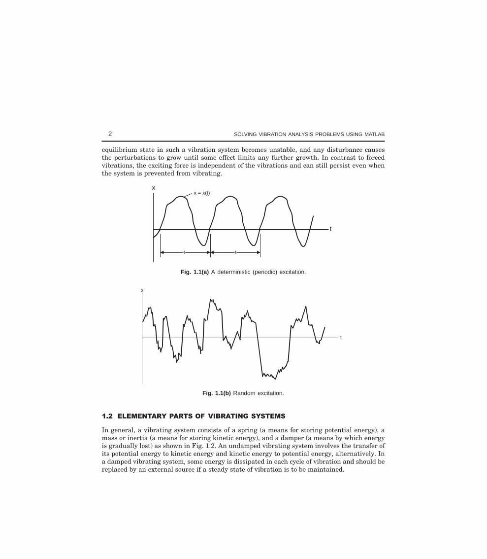
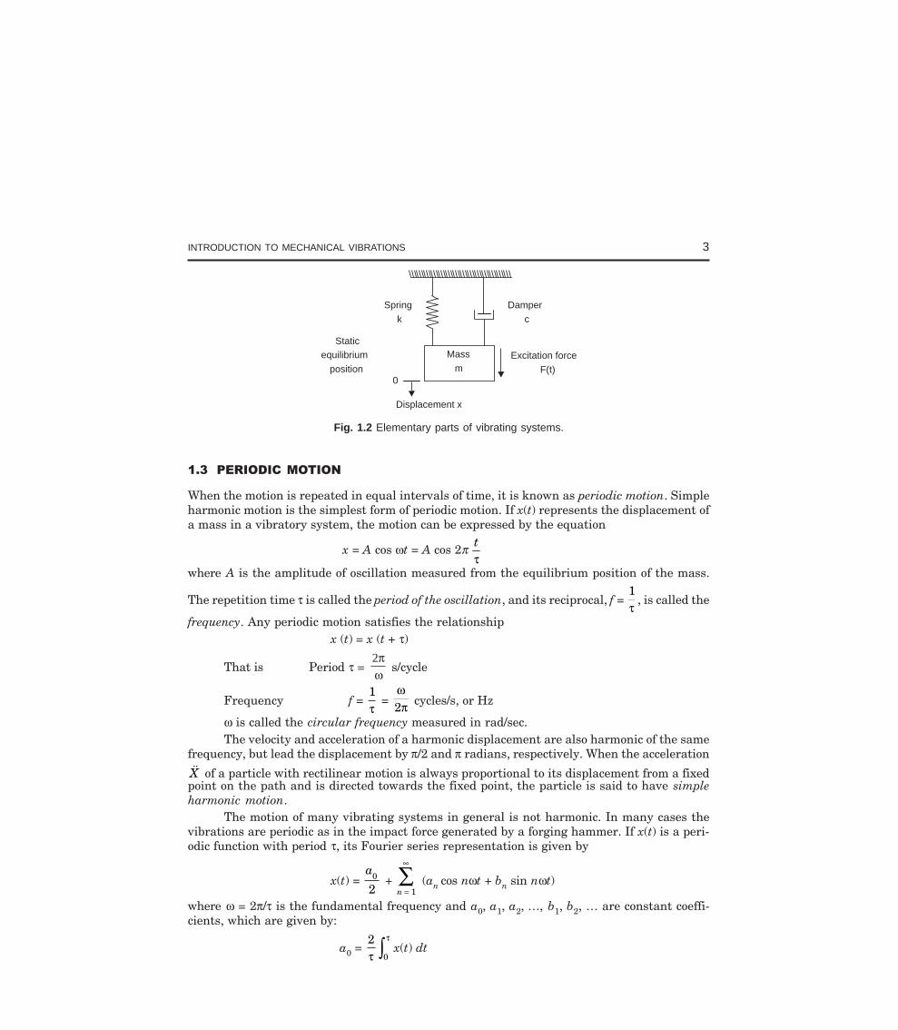
Vibrations can be classified into three categories: free, forced, and self-excited. Free vibration ofa system is vibration that occurs in the absence of external force. An external force that acts onthe system causes forced vibrations. In this case, the exciting force continuously supplies energyto the system. Forced vibrations may be either deterministic or random (see Fig. 1.1). Self-excited vibrations are periodic and deterministic oscillations. Under certain conditions, the
1
2 SOLVING VIBRATION ANALYSIS PROBLEMS USING MATLAB
equilibrium state in such a vibration system becomes unstable, and any disturbance causesthe perturbations to grow until some effect limits any further growth. In contrast to forcedvibrations, the exciting force is independent of the vibrations and can still persist even whenthe system is prevented from vibrating.
xx = x(t)
t
tt tt
Fig. 1.1(a) A deterministic (periodic) excitation.
x
t
Fig. 1.1(b) Random excitation.
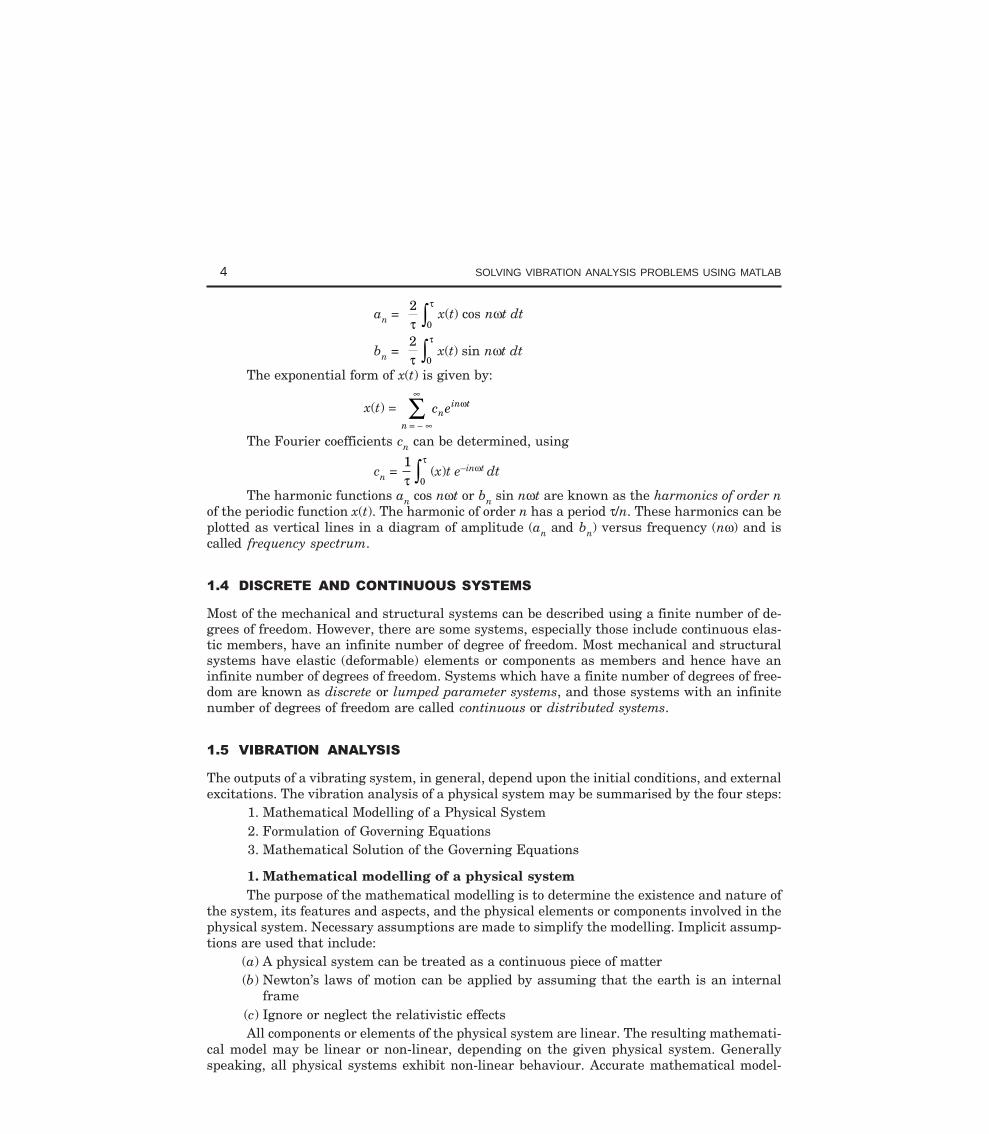
In general, a vibrating system consists of a spring (a means for storing potential energy), amass or inertia (a means for storing kinetic energy), and a damper (a means by which energyis gradually lost) as shown in Fig. 1.2. An undamped vibrating system involves the transfer ofits potential energy to kinetic energy and kinetic energy to potential energy, alternatively. Ina damped vibrating system, some energy is dissipated in each cycle of vibration and should bereplaced by an external source if a steady state of vibration is to be maintained.
INTRODUCTION TO MECHANICAL VIBRATIONS 3
Mass
m
Spring
k
Damper
c
Excitation force
F(t)0
Displacement x
Staticequilibrium
position
Fig. 1.2 Elementary parts of vibrating systems.
When the motion is repeated in equal intervals of time, it is known as periodic motion. Simpleharmonic motion is the simplest form of periodic motion. If x(t) represents the displacement ofa mass in a vibratory system, the motion can be expressed by the equation
x = A cos ωt = A cos 2π tτ
where A is the amplitude of oscillation measured from the equilibrium position of the mass.
The repetition time τ is called the period of the oscillation, and its reciprocal, f = 1τ
, is called the
frequency. Any periodic motion satisfies the relationshipx (t) = x (t + τ)
That is Period τ = ωπ2
s/cycle
Frequency f = 1τ
= ωπ2 cycles/s, or Hz
ω is called the circular frequency measured in rad/sec.The velocity and acceleration of a harmonic displacement are also harmonic of the same
frequency, but lead the displacement by π/2 and π radians, respectively. When the accelerationX of a particle with rectilinear motion is always proportional to its displacement from a fixed
point on the path and is directed towards the fixed point, the particle is said to have simpleharmonic motion.
The motion of many vibrating systems in general is not harmonic. In many cases thevibrations are periodic as in the impact force generated by a forging hammer. If x(t) is a peri-odic function with period τ, its Fourier series representation is given by
x(t) = a0
2 +
n =
∞
∑1
(an cos nωt + bn sin nωt)
where ω = 2π/τ is the fundamental frequency and a0, a1, a2, …, b1, b2, … are constant coeffi-cients, which are given by:
a0 = 2
0τ
τz x(t) dt
4 SOLVING VIBRATION ANALYSIS PROBLEMS USING MATLAB
an = 2
0τ
τz x(t) cos nωt dt
bn = 2
0τ
τz x(t) sin nωt dt
The exponential form of x(t) is given by:
x(t) = n
nin tc e
= − ∞
∞
∑ ω
The Fourier coefficients cn can be determined, using
cn = 1
0τ
τz (x)t e–inωt dt
The harmonic functions an cos nωt or bn sin nωt are known as the harmonics of order nof the periodic function x(t). The harmonic of order n has a period τ/n. These harmonics can beplotted as vertical lines in a diagram of amplitude (an and bn) versus frequency (nω) and iscalled frequency spectrum.
Most of the mechanical and structural systems can be described using a finite number of de-grees of freedom. However, there are some systems, especially those include continuous elas-tic members, have an infinite number of degree of freedom. Most mechanical and structuralsystems have elastic (deformable) elements or components as members and hence have aninfinite number of degrees of freedom. Systems which have a finite number of degrees of free-dom are known as discrete or lumped parameter systems, and those systems with an infinitenumber of degrees of freedom are called continuous or distributed systems.
The outputs of a vibrating system, in general, depend upon the initial conditions, and externalexcitations. The vibration analysis of a physical system may be summarised by the four steps:
1. Mathematical Modelling of a Physical System2. Formulation of Governing Equations3. Mathematical Solution of the Governing Equations
1. Mathematical modelling of a physical systemThe purpose of the mathematical modelling is to determine the existence and nature of
the system, its features and aspects, and the physical elements or components involved in thephysical system. Necessary assumptions are made to simplify the modelling. Implicit assump-tions are used that include:
(a) A physical system can be treated as a continuous piece of matter(b) Newton’s laws of motion can be applied by assuming that the earth is an internal
frame(c) Ignore or neglect the relativistic effectsAll components or elements of the physical system are linear. The resulting mathemati-
cal model may be linear or non-linear, depending on the given physical system. Generallyspeaking, all physical systems exhibit non-linear behaviour. Accurate mathematical model-
INTRODUCTION TO MECHANICAL VIBRATIONS 5
ling of any physical system will lead to non-linear differential equations governing the behav-iour of the system. Often, these non-linear differential equations have either no solution ordifficult to find a solution. Assumptions are made to linearise a system, which permits quicksolutions for practical purposes. The advantages of linear models are the following:
(1) their response is proportional to input(2) superposition is applicable(3) they closely approximate the behaviour of many dynamic systems(4) their response characteristics can be obtained from the form of system equations
without a detailed solution(5) a closed-form solution is often possible(6) numerical analysis techniques are well developed, and(7) they serve as a basis for understanding more complex non-linear system behaviours.It should, however, be noted that in most non-linear problems it is not possible to obtain
closed-form analytic solutions for the equations of motion. Therefore, a computer simulationis often used for the response analysis.
When analysing the results obtained from the mathematical model, one should realisethat the mathematical model is only an approximation to the true or real physical system andtherefore the actual behaviour of the system may be different.
2. Formulation of governing equationsOnce the mathematical model is developed, we can apply the basic laws of nature and
the principles of dynamics and obtain the differential equations that govern the behaviour ofthe system. A basic law of nature is a physical law that is applicable to all physical systemsirrespective of the material from which the system is constructed. Different materials behavedifferently under different operating conditions. Constitutive equations provide informationabout the materials of which a system is made. Application of geometric constraints such asthe kinematic relationship between displacement, velocity, and acceleration is often necessaryto complete the mathematical modelling of the physical system. The application of geometricconstraints is necessary in order to formulate the required boundary and/or initial conditions.
The resulting mathematical model may be linear or non-linear, depending upon thebehaviour of the elements or components of the dynamic system.
3. Mathematical solution of the governing equationsThe mathematical modelling of a physical vibrating system results in the formulation of
the governing equations of motion. Mathematical modelling of typical systems leads to a sys-tem of differential equations of motion. The governing equations of motion of a system aresolved to find the response of the system. There are many techniques available for finding thesolution, namely, the standard methods for the solution of ordinary differential equations,Laplace transformation methods, matrix methods, and numerical methods. In general, exactanalytical solutions are available for many linear dynamic systems, but for only a few non-linear systems. Of course, exact analytical solutions are always preferable to numerical orapproximate solutions.
4. Physical interpretation of the resultsThe solution of the governing equations of motion for the physical system generally
gives the performance. To verify the validity of the model, the predicted performance is com-pared with the experimental results. The model may have to be refined or a new model isdeveloped and a new prediction compared with the experimental results. Physical interpreta-
6 SOLVING VIBRATION ANALYSIS PROBLEMS USING MATLAB
tion of the results is an important and final step in the analysis procedure. In some situations,this may involve (a) drawing general inferences from the mathematical solution, (b) develop-ment of design curves, (c) arrive at a simple arithmetic to arrive at a conclusion (for a typical orspecific problem), and (d) recommendations regarding the significance of the results and anychanges (if any) required or desirable in the system involved.
1.5.1 COMPONENTS OF VIBRATING SYSTEMS
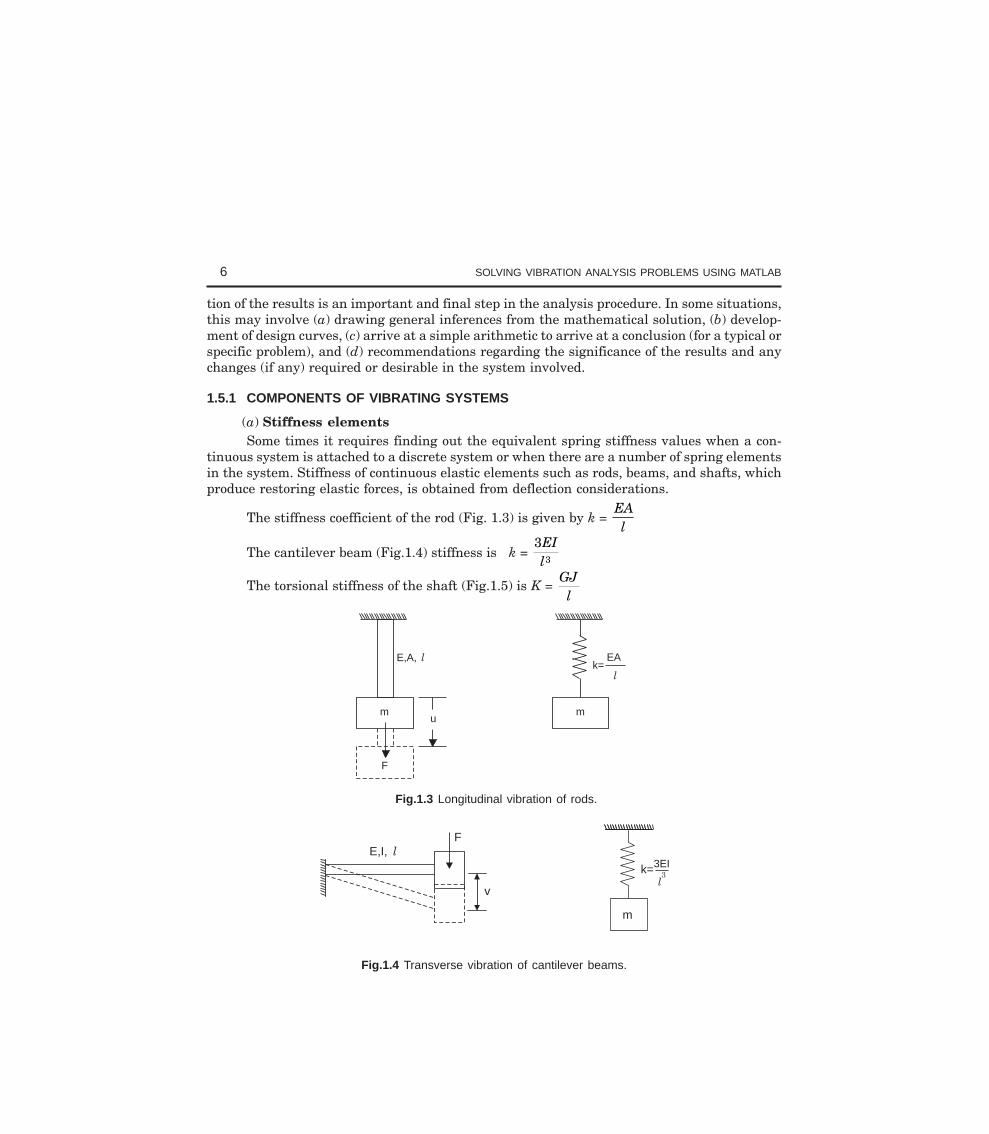
(a) Stiffness elementsSome times it requires finding out the equivalent spring stiffness values when a con-
tinuous system is attached to a discrete system or when there are a number of spring elementsin the system. Stiffness of continuous elastic elements such as rods, beams, and shafts, whichproduce restoring elastic forces, is obtained from deflection considerations.
The stiffness coefficient of the rod (Fig. 1.3) is given by k = EAl
The cantilever beam (Fig.1.4) stiffness is k = 3
3
EIl
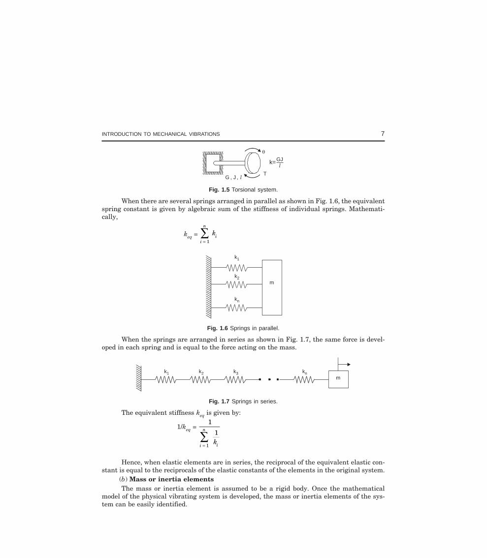
The torsional stiffness of the shaft (Fig.1.5) is K = GJ
l
m
k=l
EA
m
F
E,A, l
u
Fig.1.3 Longitudinal vibration of rods.
E,I, l
F
v
m
k=3EI
l3
Fig.1.4 Transverse vibration of cantilever beams.
INTRODUCTION TO MECHANICAL VIBRATIONS 7
G , J , lT
k=GJl
Fig. 1.5 Torsional system.
When there are several springs arranged in parallel as shown in Fig. 1.6, the equivalentspring constant is given by algebraic sum of the stiffness of individual springs. Mathemati-cally,
keq = i
n
ik=∑
1
m
k1
k2
kn
Fig. 1.6 Springs in parallel.
When the springs are arranged in series as shown in Fig. 1.7, the same force is devel-oped in each spring and is equal to the force acting on the mass.
k1 k2 k3m
kn
Fig. 1.7 Springs in series.
The equivalent stiffness keq is given by:
1/keq = 1
1
1i
n
ik=∑
Hence, when elastic elements are in series, the reciprocal of the equivalent elastic con-stant is equal to the reciprocals of the elastic constants of the elements in the original system.
(b) Mass or inertia elementsThe mass or inertia element is assumed to be a rigid body. Once the mathematical
model of the physical vibrating system is developed, the mass or inertia elements of the sys-tem can be easily identified.
8 SOLVING VIBRATION ANALYSIS PROBLEMS USING MATLAB
(c) Damping elementsIn real mechanical systems, there is always energy dissipation in one form or another.
The process of energy dissipation is referred to in the study of vibration as damping. A damperis considered to have neither mass nor elasticity. The three main forms of damping are viscousdamping, Coulomb or dry-friction damping, and hysteresis damping. The most common typeof energy-dissipating element used in vibrations study is the viscous damper, which is alsoreferred to as a dashpot. In viscous damping, the damping force is proportional to the velocityof the body. Coulomb or dry-friction damping occurs when sliding contact that exists betweensurfaces in contact are dry or have insufficient lubrication. In this case, the damping force isconstant in magnitude but opposite in direction to that of the motion. In dry-friction dampingenergy is dissipated as heat.
Solid materials are not perfectly elastic and when they are deformed, energy is absorbedand dissipated by the material. The effect is due to the internal friction due to the relativemotion between the internal planes of the material during the deformation process. Suchmaterials are known as visco-elastic solids and the type of damping which they exhibit iscalled as structural or hysteretic damping, or material or solid damping.
In many practical applications, several dashpots are used in combination. It is quitepossible to replace these combinations of dashpots by a single dashpot of an equivalent damp-ing coefficient so that the behaviour of the system with the equivalent dashpot is consideredidentical to the behaviour of the actual system.
The most basic mechanical system is the single-degree-of-freedom system, which is characterizedby the fact that its motion is described by a single variable or coordinates. Such a model isoften used as an approximation for a generally more complex system. Excitations can be broadlydivided into two types, initial excitations and externally applied forces. The behavior of asystem characterized by the motion caused by these excitations is called as the system response.The motion is generally described by displacements.
1.6.1 FREE VIBRATION OF AN UNDAMPED TRANSLATIONAL SYSTEM
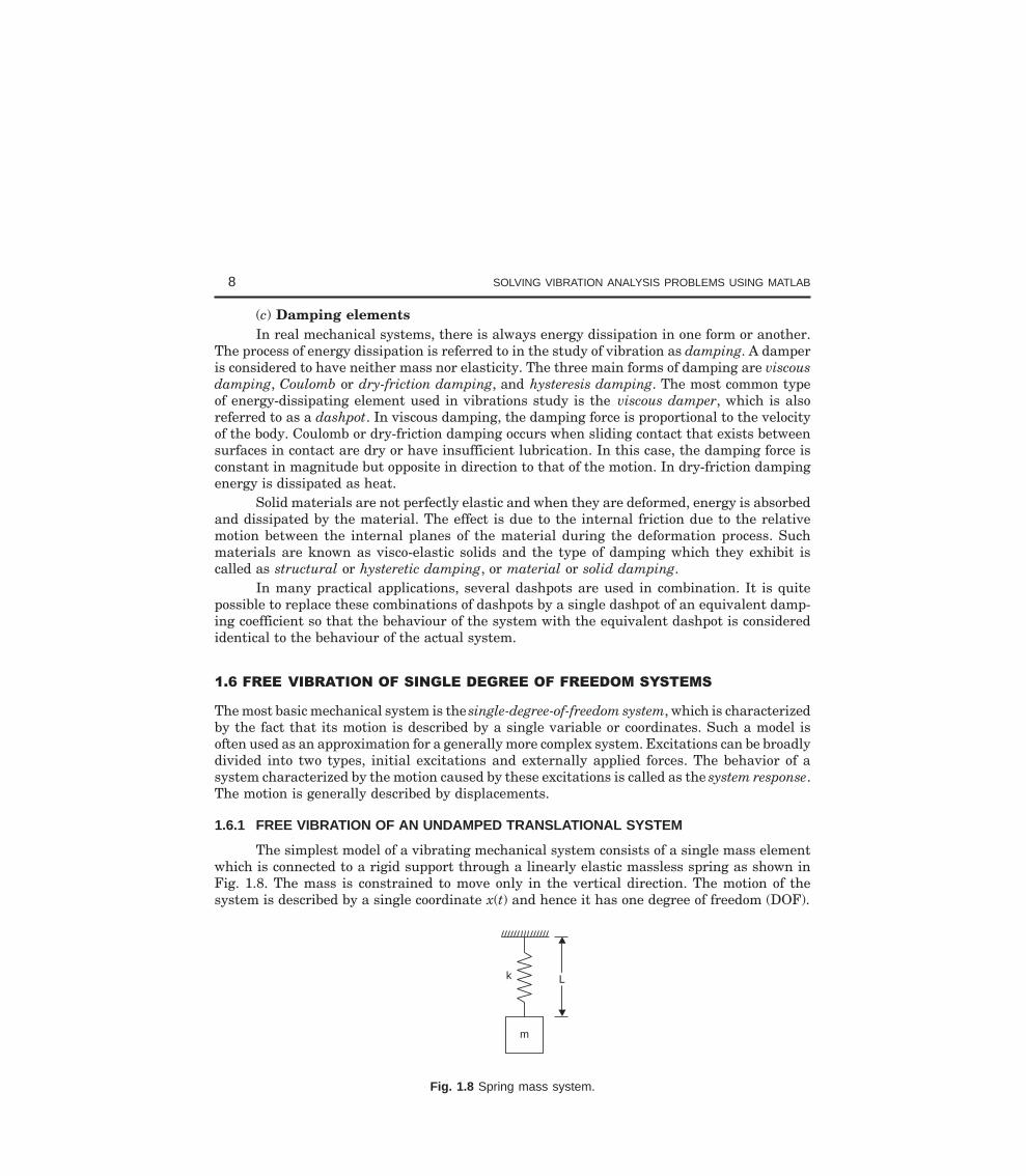
The simplest model of a vibrating mechanical system consists of a single mass elementwhich is connected to a rigid support through a linearly elastic massless spring as shown inFig. 1.8. The mass is constrained to move only in the vertical direction. The motion of thesystem is described by a single coordinate x(t) and hence it has one degree of freedom (DOF).
m
k LL
Fig. 1.8 Spring mass system.
INTRODUCTION TO MECHANICAL VIBRATIONS 9
The equation of motion for the free vibration of an undamped single degree of freedomsystem can be rewritten as
m x(t) + kx (t) = 0Dividing through by m, the equation can be written in the form
x(t) + ω n2 x (t) = 0
in which ωn = k m/ is a real constant. The solution of this equation is obtained from the initialconditions
x(0) = x0, x(0) = v0where x0 and v0 are the initial displacement and initial velocity, respectively.
The general solution can be written as
x(t) = A1e A ei t i nt
nω ω+ −2
in which A1 and A2 are constants of integration, both complex quantities. It can be finallysimplified as:
x(t) = X
e ei t i tn n
2( ) ( )ω φ ω φ− − −+ = X cos (ωnt – φ)
so that now the constants of integration are X and φ.This equation represents harmonic oscillation, for which reason such a system is called
a harmonic oscillator.There are three quantities defining the response, the amplitude X, the phase angle φ
and the frequency ωn, the first two depending on external factors, namely, the initial excitations,and the third depending on internal factors, namely, the system parameters. On the otherhand, for a given system, the frequency of the response is a characteristic of the system thatstays always the same, independently of the initial excitations. For this reason, ωn is called thenatural frequency of the harmonic oscillator.
The constants X and φ are obtained from the initial conditions of the system as follows:
X = xv
n02 0
2
+FHG
IKJω
and φ = tan–1 v
x n
0
0ω
LNMM
OQPP
The time period τ, is defined as the time necessary for the system to complete one vibra-tion cycle, or as the time between two consecutive peaks. It is related to the natural frequencyby
τ = 22
πω
πn
mk
=
Note that the natural frequency can also be defined as the reciprocal of the period, or
fn = 1 12τ π
=km
in which case it has units of cycles per second (cps), where one cycle per second is known as oneHertz (Hz).

10 SOLVING VIBRATION ANALYSIS PROBLEMS USING MATLAB
1.6.2 FREE VIBRATION OF AN UNDAMPED TORSIONAL SYSTEM
A mass attached to the end of the shaft is a simple torsional system (Fig. 1.9). The massof the shaft is considered to be small in comparison to the mass of the disk and is thereforeneglected.
kt
l
IG
Fig. 1.9 Torsional system.
The torque that produces the twist Mt is given by
Mt = GJ
l
where J = the polar mass moment of inertia of the shaft Jd=
FHG
π 4
32 for a circular shaft of
diameter dIK
G = shear modulus of the material of the shaft.l = length of the shaft.
The torsional spring constant kt is defined as
kt = T GJ
lθ=
The equation of motion of the system can be written as:
IGθ + ktθ = 0
The natural circular frequency of such a torsional system is ωn = k
It
G
FHG
IKJ
1/2
The general solution of equation of motion is given by
θ(t) = θ0 cos ωnt + θω
0
n
sin ωnt
1.6.3 ENERGY METHOD
Free vibration of systems involves the cyclic interchange of kinetic and potential energy. Inundamped free vibrating systems, no energy is dissipated or removed from the system. Thekinetic energy T is stored in the mass by virtue of its velocity and the potential energy U isstored in the form of strain energy in elastic deformation. Since the total energy in the system
INTRODUCTION TO MECHANICAL VIBRATIONS 11
is constant, the principle of conservation of mechanical energy applies. Since the mechanicalenergy is conserved, the sum of the kinetic energy and potential energy is constant and its rateof change is zero. This principle can be expressed as
T + U = constant
orddt
(T + U) = 0
where T and U denote the kinetic and potential energy, respectively. The principle of conser-vation of energy can be restated by
T1 + U1 = T2 + U2where the subscripts 1 and 2 denote two different instances of time when the mass is passingthrough its static equilibrium position and select U1 = 0 as reference for the potential energy.Subscript 2 indicates the time corresponding to the maximum displacement of the mass at thisposition, we have then
T2 = 0and T1 + 0 = 0 + U2
If the system is undergoing harmonic motion, then T1 and U2 denote the maximumvalues of T and U, respectively and therefore last equation becomes
Tmax = Umax
It is quite useful in calculating the natural frequency directly.
1.6.4 STABILITY OF UNDAMPED LINEAR SYSTEMS
The mass/inertia and stiffness parameters have an affect on the stability of an undampedsingle degree of freedom vibratory system. The mass and stiffness coefficients enter into thecharacteristic equation which defines the response of the system. Hence, any changes in thesecoefficient will lead to changes in the system behavior or response. In this section, the effectsof the system inertia and stiffness parameters on the stability of the motion of an undampedsingle degree of freedom system are examined. It can be shown that by a proper selection ofthe inertia and stiffness coefficients, the instability of the motion of the system can be avoided.A stable system is one which executes bounded oscillations about the equilibrium position.
1.6.5 FREE VIBRATION WITH VISCOUS DAMPING
Viscous damping force is proportional to the velocity x of the mass and acting in thedirection opposite to the velocity of the mass and can be expressed as
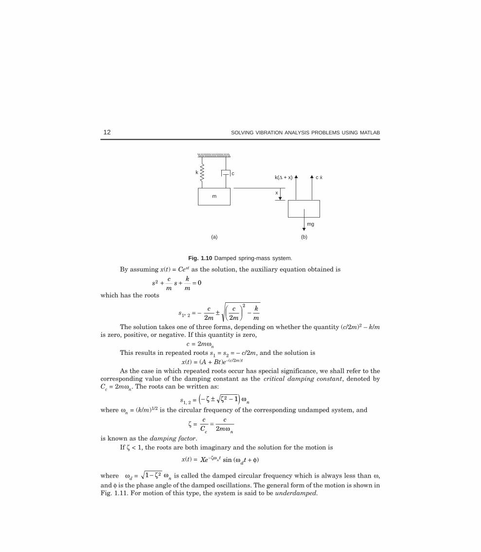
F = c xwhere c is the damping constant or coefficient of viscous damping. The differential equation ofmotion for free vibration of a damped spring-mass system (Fig. 1.10) is written as:
xcm
xkm
x+ + = 0
12 SOLVING VIBRATION ANALYSIS PROBLEMS USING MATLAB
(a) (b)
k c
mx
k( + x) c x.
mg
Fig. 1.10 Damped spring-mass system.
By assuming x(t) = Cest as the solution, the auxiliary equation obtained is
scm
skm
2 0+ + =
which has the roots
s1, 2 = – cm
cm
km2 2
2
± FHG
IKJ −
The solution takes one of three forms, depending on whether the quantity (c/2m)2 – k/mis zero, positive, or negative. If this quantity is zero,
c = 2mωnThis results in repeated roots s1 = s2 = – c/2m, and the solution is
x(t) = (A + Bt)e–(c/2m)t
As the case in which repeated roots occur has special significance, we shall refer to thecorresponding value of the damping constant as the critical damping constant, denoted byCc = 2mωn. The roots can be written as:
s1, 2 = − ± −ζ ζ ω2 1e j n
where ωn = (k/m)1/2 is the circular frequency of the corresponding undamped system, and
ζ = c
Cc
mc n
=2 ω
is known as the damping factor.If ζ < 1, the roots are both imaginary and the solution for the motion is
x(t) = Xe tntd
− +ζω ω φsin ( )
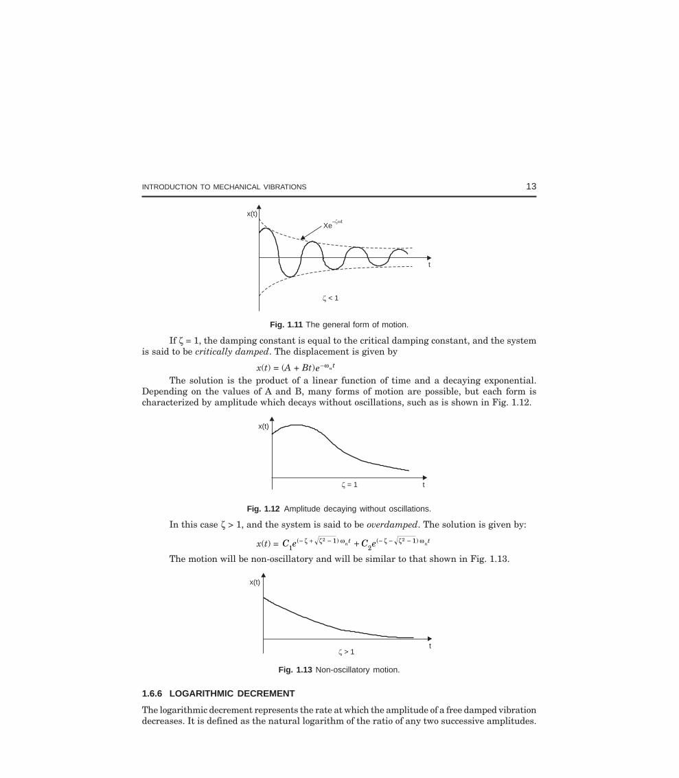
where ωd = 1 2− ζ ωn is called the damped circular frequency which is always less than ω,and φ is the phase angle of the damped oscillations. The general form of the motion is shown inFig. 1.11. For motion of this type, the system is said to be underdamped.
INTRODUCTION TO MECHANICAL VIBRATIONS 13
x(t)
Xe– t
< 1
t
Fig. 1.11 The general form of motion.
If ζ = 1, the damping constant is equal to the critical damping constant, and the systemis said to be critically damped. The displacement is given by
x(t) = (A + Bt)e nt−ω
The solution is the product of a linear function of time and a decaying exponential.Depending on the values of A and B, many forms of motion are possible, but each form ischaracterized by amplitude which decays without oscillations, such as is shown in Fig. 1.12.
t
x(t)
= 1
Fig. 1.12 Amplitude decaying without oscillations.
In this case ζ > 1, and the system is said to be overdamped. The solution is given by:
x(t) = C e C en nt t1
12
12 2( ) ( )− + − − − −+ζ ζ ω ζ ζ ω
The motion will be non-oscillatory and will be similar to that shown in Fig. 1.13.
t
x(t)
> 1
Fig. 1.13 Non-oscillatory motion.
1.6.6 LOGARITHMIC DECREMENT
The logarithmic decrement represents the rate at which the amplitude of a free damped vibrationdecreases. It is defined as the natural logarithm of the ratio of any two successive amplitudes.
14 SOLVING VIBRATION ANALYSIS PROBLEMS USING MATLAB
The ratio of successive amplitudes is
x
xXe
Xei
i
t
t
n i
n i d+
−
− +=1
ζω
ζω τ( ) = e n dζω τ = constant
The logarithmic decrement
δ = lnx
xei
in d
n d
+
= =1
ln ζω τ ζω τ
Substituting τd = 2π/ωd = 2π/ωn 1 2− ζ gives
δ = 2
1 2
πζζ−
1.6.7 TORSIONAL SYSTEM WITH VISCOUS DAMPING
The equation of motion for such a system can be written as
Iθ + ctθ + ktθ = 0
where I is the mass moment of inertia of the disc, kt is the torsional spring constant (restoringtorque for unit angular displacement), and θ is the angular displacement of the disc.
1.6.8 FREE VIBRATION WITH COULOMB DAMPING
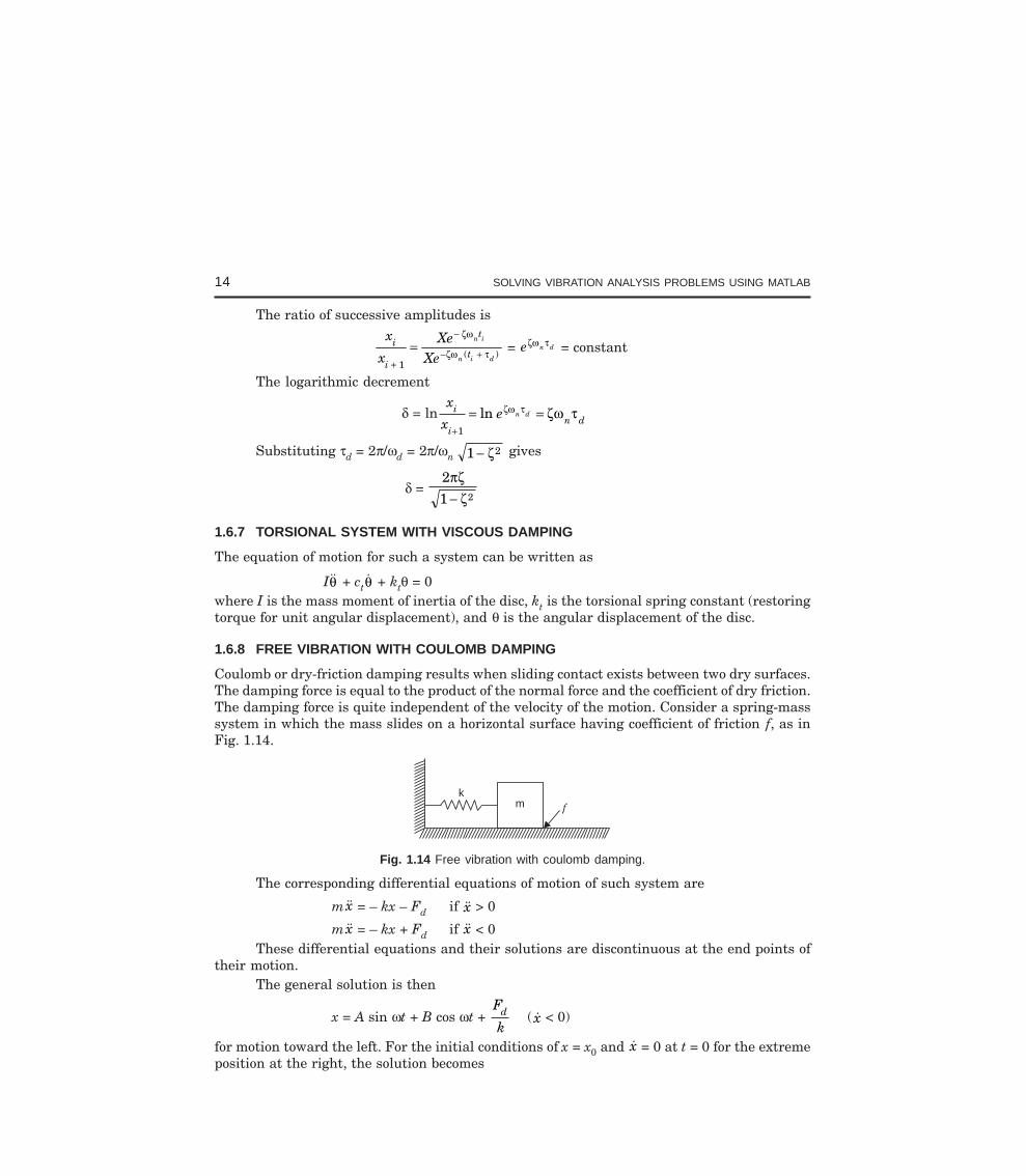
Coulomb or dry-friction damping results when sliding contact exists between two dry surfaces.The damping force is equal to the product of the normal force and the coefficient of dry friction.The damping force is quite independent of the velocity of the motion. Consider a spring-masssystem in which the mass slides on a horizontal surface having coefficient of friction f, as inFig. 1.14.
km
f
Fig. 1.14 Free vibration with coulomb damping.
The corresponding differential equations of motion of such system are
m x = – kx – Fd if x > 0
m x = – kx + Fd if x < 0These differential equations and their solutions are discontinuous at the end points of
their motion.The general solution is then
x = A sin ωt + B cos ωt + F
kd ( x < 0)
for motion toward the left. For the initial conditions of x = x0 and x = 0 at t = 0 for the extremeposition at the right, the solution becomes
INTRODUCTION TO MECHANICAL VIBRATIONS 15
x = xF
kt
F
kd d
0 −FHG
IKJ +cos ω ( x < 0)
This holds for motion toward the left, or until x again becomes zero.Hence the displacement is negative, or to the left of the neutral position, and has a
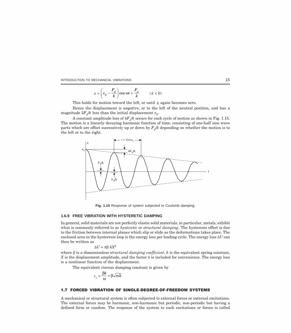
magnitude 2Fd/k less than the initial displacement x0.A constant amplitude loss of 4Fd/k occurs for each cycle of motion as shown in Fig. 1.15.
The motion is a linearly decaying harmonic function of time, consisting of one-half sine waveparts which are offset successively up or down by Fd/k depending on whether the motion is tothe left or to the right.
x
x0 4F /kd
= 2 / n
F /kd
F /kd
t
Fig. 1.15 Response of system subjected to Coulomb damping.
1.6.9 FREE VIBRATION WITH HYSTERETIC DAMPING
In general, solid materials are not perfectly elastic solid materials, in particular, metals, exhibitwhat is commonly referred to as hysteretic or structural damping. The hysteresis effect is dueto the friction between internal planes which slip or slide as the deformations takes place. Theenclosed area in the hysteresis loop is the energy loss per loading cycle. The energy loss ∆U canthen be written as
∆U = πβ kX2
where β is a dimensionless structural damping coefficient, k is the equivalent spring constant,X is the displacement amplitude, and the factor π is included for convenience. The energy lossis a nonlinear function of the displacement.
The equivalent viscous damping constant is given by
ce = βω
βkmk=
A mechanical or structural system is often subjected to external forces or external excitations.The external forces may be harmonic, non-harmonic but periodic, non-periodic but having adefined form or random. The response of the system to such excitations or forces is called
16 SOLVING VIBRATION ANALYSIS PROBLEMS USING MATLAB
forced response. The response of a system to a harmonic excitation is called harmonic response.The non-periodic excitations may have a long or short duration. The response of a system tosuddenly applied non-periodic excitations is called transient response. The sources of harmonicexcitations are unbalance in rotating machines, forces generated by reciprocating machines,and the motion of the machine itself in certain cases.
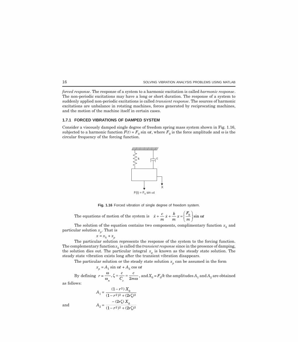
1.7.1 FORCED VIBRATIONS OF DAMPED SYSTEM
Consider a viscously damped single degree of freedom spring mass system shown in Fig. 1.16,subjected to a harmonic function F(t) = F0 sin ωt, where F0 is the force amplitude and ω is thecircular frequency of the forcing function.
ck
F(t) = F sin t0
X
Fig. 1.16 Forced vibration of single degree of freedom system.
The equations of motion of the system is sinxcm
xkm
xF
mt+ + =
FHG
IKJ
0 ω
The solution of the equation contains two components, complimentary function xh andparticular solution xp. That is
x = xh + xpThe particular solution represents the response of the system to the forcing function.
The complementary function xh is called the transient response since in the presence of damping,the solution dies out. The particular integral xp is known as the steady state solution. Thesteady state vibration exists long after the transient vibration disappears.
The particular solution or the steady state solution xp can be assumed in the formxp = A1 sin ωt + A2 cos ωt
By defining r = ω
ωζ
ωn c
cC
cm
, = =2
, and X0 = F0/k the amplitudes A1 and A2 are obtained
as follows:
A1 = ( )
( ) ( )
1
1 2
20
2 2 2
−− +
r X
r rζ
and A2 = −
− +( )
( ) ( )
2
1 20
2 2 2
r X
r r
ζζ
INTRODUCTION TO MECHANICAL VIBRATIONS 17
The steady state solution xp can be written as
xp = X
r rr t r t0
2 2 22
1 21 2
( ) ( )[( ) sin ( ) cos ]
−− −
ζω ζ ω
which can also be written as
xp = X
r rt0
2 2 21 2( ) ( )sin ( )
−−
ζω φ
where X0 is the forced amplitude and φ is the phase angle defined by
φ = tan−−
FHG
IKJ
12
21
rrζ
It can be written in a more compact form asxp = X0β sin (ωt – φ)
where β is known as magnification factor. For damped systems β is defined as
β = 1
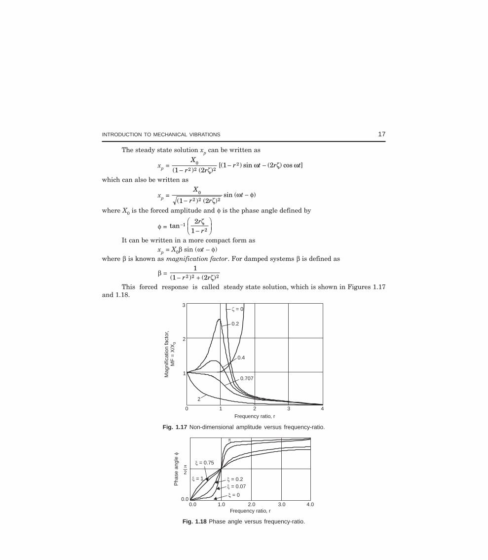
1 22 2 2( ) ( )− +r rζThis forced response is called steady state solution, which is shown in Figures 1.17
and 1.18.
0 1 2 3 4
1
2
3 = 0
0.2
0.4
0.707
2
Mag
nific
atio
nfa
ctor
,M
F=
X/X
0
Frequency ratio, r
Fig. 1.17 Non-dimensional amplitude versus frequency-ratio.
0.00.0 1.0 2.0 3.0 4.0
Pha
sean
gle
2
p
= 0.75
= 1 = 0.2 = 0.07
= 0
Frequency ratio, r
Fig. 1.18 Phase angle versus frequency-ratio.
18 SOLVING VIBRATION ANALYSIS PROBLEMS USING MATLAB
The magnification factor β is found to be maximum when
r = 1 2 2− ζ
The maximum magnification factor is given by:
βmax = 1
2 1 2ζ ζ−In the undamped systems, the particular solution reduces to
xp(t) =
F
k t
n
0
2
1 −FHG
IKJ
L
NMM
O
QPP
ωω
ωsin
The maximum amplitude can also be expressed asX
st
n
δ ωω
=
−FHG
IKJ
1
12
where δst = F0/k denotes the static deflection of the mass under a force F0 and is sometimesknow as static deflection since F0 is a constant static force. The quantity X/δst represents theratio of the dynamic to the static amplitude of motion and is called the magnification factor,amplification factor, or amplitude ratio.
1.7.1.1 Resonance
The case r = ω
ω n
= 1, that is, when the circular frequency of the forcing function is equal to the
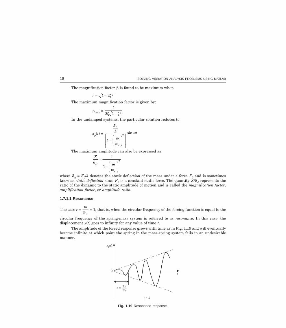
circular frequency of the spring-mass system is referred to as resonance. In this case, thedisplacement x(t) goes to infinity for any value of time t.
The amplitude of the forced response grows with time as in Fig. 1.19 and will eventuallybecome infinite at which point the spring in the mass-spring system fails in an undesirablemanner.
t
x (t)p
0
r = 1
= 2n
Fig. 1.19 Resonance response.
INTRODUCTION TO MECHANICAL VIBRATIONS 19
1.7.2 BEATS
The phenomenon of beating occurs for an undamped forced single degree of freedom spring-mass system when the forcing frequency ω is close, but not equal, to the system circularfrequency ωn. In this case, the amplitude builds up and then diminishes in a regular pattern.The phenomenon of beating can be noticed in cases of audio or sound vibration and in electricpower generation when a generator is started.
1.7.3 TRANSMISSIBILITY
The forces associated with the vibrations of a machine or a structure will be transmitted to itssupport structure. These transmitted forces in most instances produce undesirable effects suchas noise. Machines and structures are generally mounted on designed flexible supports knownas vibration isolators or isolators.
In general, the amplitude of vibration reduces with the increasing values of the springstiffness k and the damping coefficient c. In order to reduce the force transmitted to the sup-port structure, a proper selection of the stiffness and damping coefficients must be made.
From regular spring-mass-damper model, force transmitted to the support can be writ-ten as
FT = k xp + c xp= X0β k c t2 2+ −( ) sin ( )ω ω φ
where φ = φ – φt
and φt is the phase angle defined as
φt = tan–1 ckωF
HGIKJ = tan–1(2rζ)
Transmitted force can also be written as:
FT = F0βt sin (ωt – φ )
where βt = 1 2
1 2
2
2 2 2
+− +
( )
( ) ( )
r
r r
ζζ
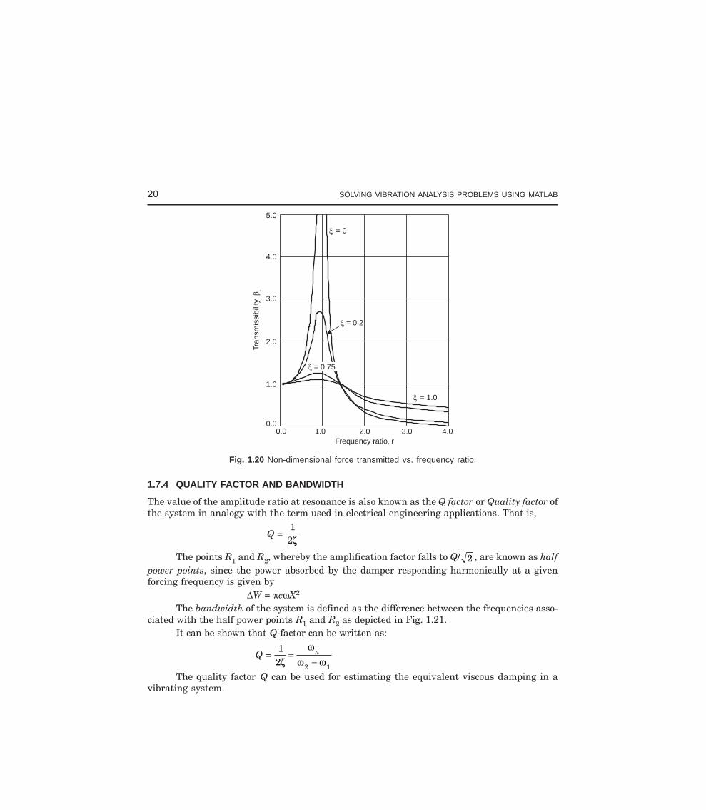
The transmissibility βt is defined as the ratio of the maximum transmitted force to theamplitude of the applied force. Fig. 1.20 shows a plot of βt versus the frequency ratio r fordifferent values of the damping factor ζ.
It can be observed from Fig. 1.20, that β > 1 for r < 2 which means that in this regionthe amplitude of the transmitted force is greater than the amplitude of the applied force. Also,the r < 2 , the transmitted force to the support can be reduced by increasing the damping
factor ζ. For r = 2 , every curve passes through the point βt = 1 and becomes asymptotic to
zero as the frequency ratio is increased. Similarly, for r > 2 , βt < 1, hence, in this region theamplitude of the transmitted force is less than the amplitude of the applied force. Therefore,the amplitude of the transmitted force increases by increasing the damping factor ζ. Thus,vibration isolation is best accomplished by an isolator composed only of spring-elements forwhich r > 2 with no damping element used in the system.
20 SOLVING VIBRATION ANALYSIS PROBLEMS USING MATLAB
= 0
= 0.2
= 1.0
0.0 1.0 2.0 4.03.00.0
1.0
2.0
3.0
4.0
5.0
= 0.75
Tran
smis
sibi
lity,
t
Frequency ratio, r
Fig. 1.20 Non-dimensional force transmitted vs. frequency ratio.
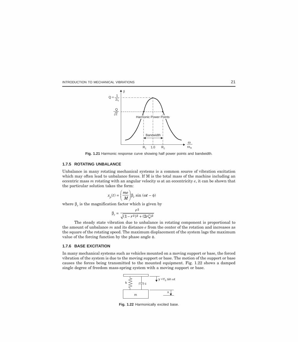
1.7.4 QUALITY FACTOR AND BANDWIDTH
The value of the amplitude ratio at resonance is also known as the Q factor or Quality factor ofthe system in analogy with the term used in electrical engineering applications. That is,
Q = 1
2ζ
The points R1 and R2, whereby the amplification factor falls to Q/ 2 , are known as halfpower points, since the power absorbed by the damper responding harmonically at a givenforcing frequency is given by
∆W = πcωX2
The bandwidth of the system is defined as the difference between the frequencies asso-ciated with the half power points R1 and R2 as depicted in Fig. 1.21.
It can be shown that Q-factor can be written as:
Q = 1
2 2 1ζω
ω ω=
−n
The quality factor Q can be used for estimating the equivalent viscous damping in avibrating system.
INTRODUCTION TO MECHANICAL VIBRATIONS 21
R1 R21.0
b
Q = 12
nww
BandwidthBandwidth
Q2
Harmonic Power PointsHarmonic Power Points
Fig. 1.21 Harmonic response curve showing half power points and bandwidth.
1.7.5 ROTATING UNBALANCE
Unbalance in many rotating mechanical systems is a common source of vibration excitationwhich may often lead to unbalance forces. If M is the total mass of the machine including aneccentric mass m rotating with an angular velocity ω at an eccentricity e, it can be shown thatthe particular solution takes the form:
xp(t) = meM
FHG
IKJ βr sin (ωt – φ)
where βr is the magnification factor which is given by
βr = r
r r
2
2 2 21 2( ) ( )− + ζThe steady state vibration due to unbalance in rotating component is proportional to
the amount of unbalance m and its distance e from the center of the rotation and increases asthe square of the rotating speed. The maximum displacement of the system lags the maximumvalue of the forcing function by the phase angle φ.
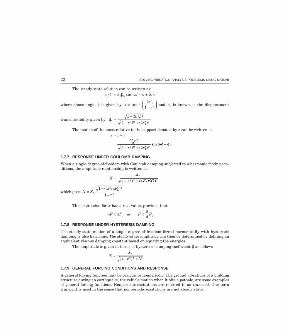
1.7.6 BASE EXCITATION
In many mechanical systems such as vehicles mounted on a moving support or base, the forcedvibration of the system is due to the moving support or base. The motion of the support or basecauses the forces being transmitted to the mounted equipment. Fig. 1.22 shows a dampedsingle degree of freedom mass-spring system with a moving support or base.
m
c
x
ky =Y sin t0
Fig. 1.22 Harmonically excited base.
22 SOLVING VIBRATION ANALYSIS PROBLEMS USING MATLAB
The steady state solution can be written as:xp(t) = Y0βb sin (ωt – φ + φb),
where phase angle φ is given by φ = tan–1 21 2
rrζ
−FHG
IKJ and βb is known as the displacement
transmissibility given by: βb = 1 2
1 2
2
2 2 2
+− +
( )
( ) ( )
r
r r
ζζ
The motion of the mass relative to the support denoted by z can be written asz = x – y
= Y r
r rt0
2
2 2 21 2( ) ( )sin ( )
− +−
ζω φ
1.7.7 RESPONSE UNDER COULOMB DAMPING
When a single-degree-of-freedom with Coulomb damping subjected to a harmonic forcing con-ditions, the amplitude relationship is written as:
X = X
r F Xk0
2 2 21 4( ) ( / )− + π
which gives X = X0
1 4
10
2
2
−
−
( / )F F
r
π
This expression for X has a real value, provided that
4F < πF0 or F < π4
F0
1.7.8 RESPONSE UNDER HYSTERESIS DAMPING
The steady-state motion of a single degree of freedom forced harmonically with hysteresisdamping is also harmonic. The steady-state amplitude can then be determined by defining anequivalent viscous damping constant based on equating the energies.
The amplitude is given in terms of hysteresis damping coefficient β as follows
X = X
r0
2 2 21( )− + β
1.7.9 GENERAL FORCING CONDITIONS AND RESPONSE
A general forcing function may be periodic or nonperiodic. The ground vibrations of a buildingstructure during an earthquake, the vehicle motion when it hits a pothole, are some examplesof general forcing functions. Nonperiodic excitations are referred to as transient. The termtransient is used in the sense that nonperiodic excitations are not steady state.
INTRODUCTION TO MECHANICAL VIBRATIONS 23
1.7.10 FOURIER SERIES AND HARMONIC ANALYSIS
The Fourier series expression of a given periodic function F(t) with period T can be expressedin terms of harmonic functions as
F(t) = a
a n t b n tn
nn
n0
1 12+ +
=
∞
=
∞
∑ ∑cos sinω ω
where ω = 2πT
and a0, an and bn are constants.
F(t) can also be written as follows:
F(t) = F0 + n
n n nF t=
∞
∑ +1
sin ( )ω φ
where F0 = a0/2, Fn = a bn n2 2+ , with ωn = nω and φn = tan–1
a
bn
n
FHG
IKJ
Harmonic functions are periodic functions in which all the Fourier coefficients are zeros exceptone coefficient.
1.8.1 EVEN FUNCTIONS
A periodic function F(t) is said to be even if F(t) = F(– t). A cosine function is an even functionsince cos θ = cos (– θ). If the function F(t) is an even function, then the coefficients bm are allzeros.
1.8.2 ODD FUNCTIONS
A periodic function F(t) is said to be odd if F(t) = – F(– t). The sine function is an odd functionsince sin θ = – sin(– θ). For an odd function, the Fourier coefficients a0 and an are identicallyzero.
1.8.3 RESPONSE UNDER A PERIODIC FORCE OF IRREGULAR FORM
Usually, the values of periodic functions at discrete points in time are available in graphicalform or tabulated form. In such cases, no analytical expression can be found or the directintegration of the periodic functions in a closed analytical form may not be practical. In suchcases, one can find the Fourier coefficients by using a numerical integration procedure. If onedivides the period of the function T into N equal intervals, then length of each such interval is∆t = T/N.
The coefficients are given by
a0 = 2
1NF t
i
N
i=∑ ( )
24 SOLVING VIBRATION ANALYSIS PROBLEMS USING MATLAB
an = 2
1NF t
i
N
i=∑ ( ) cos nωti
bn = 2
1NF t
i
N
i=∑ ( ) sin nωti
1.8.4 RESPONSE UNDER A GENERAL PERIODIC FORCE
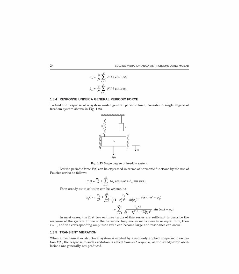
To find the response of a system under general periodic force, consider a single degree offreedom system shown in Fig. 1.23.
m
ck
F(t)
x
Fig. 1.23 Single degree of freedom system.
Let the periodic force F(t) can be expressed in terms of harmonic functions by the use ofFourier series as follows:
F(t) = a
n
0
12+
=
∞
∑ (an cos nωt + bn sin nωt)
Then steady-state solution can be written as
xp(t) = a
k
a k
r rn
n
n n
0
12 2 22 1 2
+− +=
∞
∑ /
( ) ( )ξ cos (nωt – ψn)
+ n
n
n n
b k
r r=
∞
∑ − +12 2 21 2
/
( ) ( )ξ sin (nωt – ψn)
In most cases, the first two or three terms of this series are sufficient to describe theresponse of the system. If one of the harmonic frequencies nω is close to or equal to ω, thenr ≈ 1, and the corresponding amplitude ratio can become large and resonance can occur.
1.8.5 TRANSIENT VIBRATION
When a mechanical or structural system is excited by a suddenly applied nonperiodic excita-tion F(t), the response to such excitation is called transient response, as the steady-state oscil-lations are generally not produced.
INTRODUCTION TO MECHANICAL VIBRATIONS 25
1.8.6 UNIT IMPULSE
Impulse is time integral of the force which is finite and is written asF = ∫ F(t) dt
where F is the linear impulse (in pound seconds or Newton seconds) of the force.
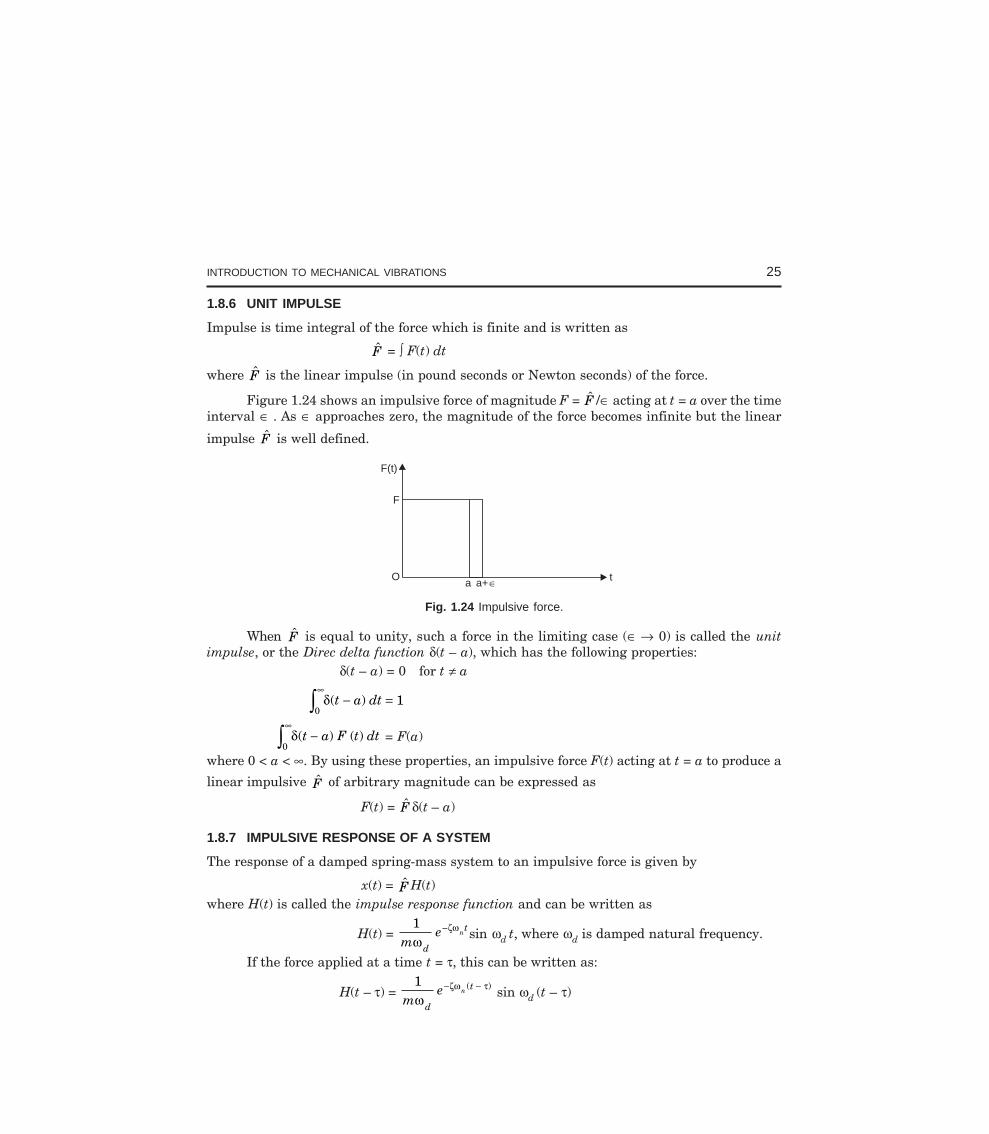
Figure 1.24 shows an impulsive force of magnitude F = F /∈ acting at t = a over the timeinterval ∈ . As ∈ approaches zero, the magnitude of the force becomes infinite but the linear
impulse F is well defined.
t
F
F(t)
Oa a+
Fig. 1.24 Impulsive force.
When F is equal to unity, such a force in the limiting case (∈ → 0) is called the unitimpulse, or the Direc delta function δ(t – a), which has the following properties:
δ(t – a) = 0 for t ≠ a
01
∞z − =δ( )t a dt
0
∞z −δ( ) ( )t a F t dt = F(a)
where 0 < a < ∞. By using these properties, an impulsive force F(t) acting at t = a to produce a
linear impulsive F of arbitrary magnitude can be expressed as
F(t) = F δ(t – a)
1.8.7 IMPULSIVE RESPONSE OF A SYSTEM
The response of a damped spring-mass system to an impulsive force is given by
x(t) = F H(t)where H(t) is called the impulse response function and can be written as
H(t) = 1
me
d
tn
ωζω− sin ωd t, where ωd is damped natural frequency.
If the force applied at a time t = τ, this can be written as:
H(t – τ) = 1
me
d
tn
ωζω τ− −( ) sin ωd (t – τ)
26 SOLVING VIBRATION ANALYSIS PROBLEMS USING MATLAB
1.8.8 RESPONSE TO AN ARBITRARY INPUT
The total response is obtained by finding the integration
x(t) = 0
tF H t dz −( ) ( )τ τ τ
This is called the convolution integral or Duhamel’s integral and is sometimes referred as thesuperposition integral.
1.8.9 LAPLACE TRANSFORMATION METHOD
The Laplace transformation method can be used for calculating the response of a system to avariety of force excitations, including periodic and nonperiodic. The Laplace transformationmethod can treat discontinuous functions with no difficulty and it automatically takes intoaccount the initial conditions. The usefulness of the method lies in the availability of tabulatedLaplace transform pairs. From the equations of motion of a single degree of freedom systemsubjected to a general forcing function F(t), the Laplace transform of the solution x(t) is givenby
x sF s ms c x mx
ms cs k( )
( ) ( ) ( ) ( )= + + ++ +
0 02
The method of determining x(t) given x s( ) can be considered as an inverse transforma-tion which can be expressed as
x(t) = L–1 ( )x s
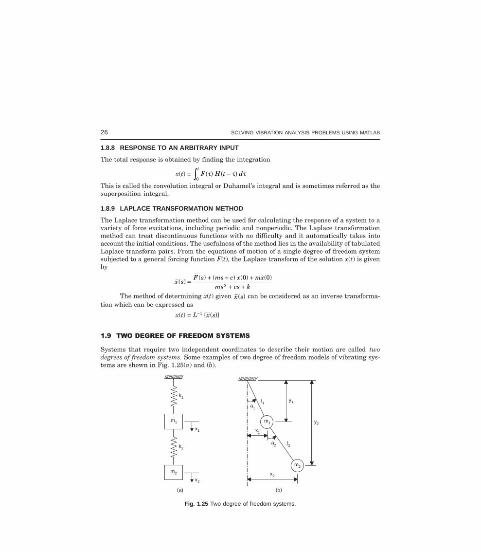
Systems that require two independent coordinates to describe their motion are called twodegrees of freedom systems. Some examples of two degree of freedom models of vibrating sys-tems are shown in Fig. 1.25(a) and (b).
m1
m2
k1
x1
l11
y1
y2
x2
k2l22
x1
x2
m2
m1
(a) (b)
Fig. 1.25 Two degree of freedom systems.
INTRODUCTION TO MECHANICAL VIBRATIONS 27
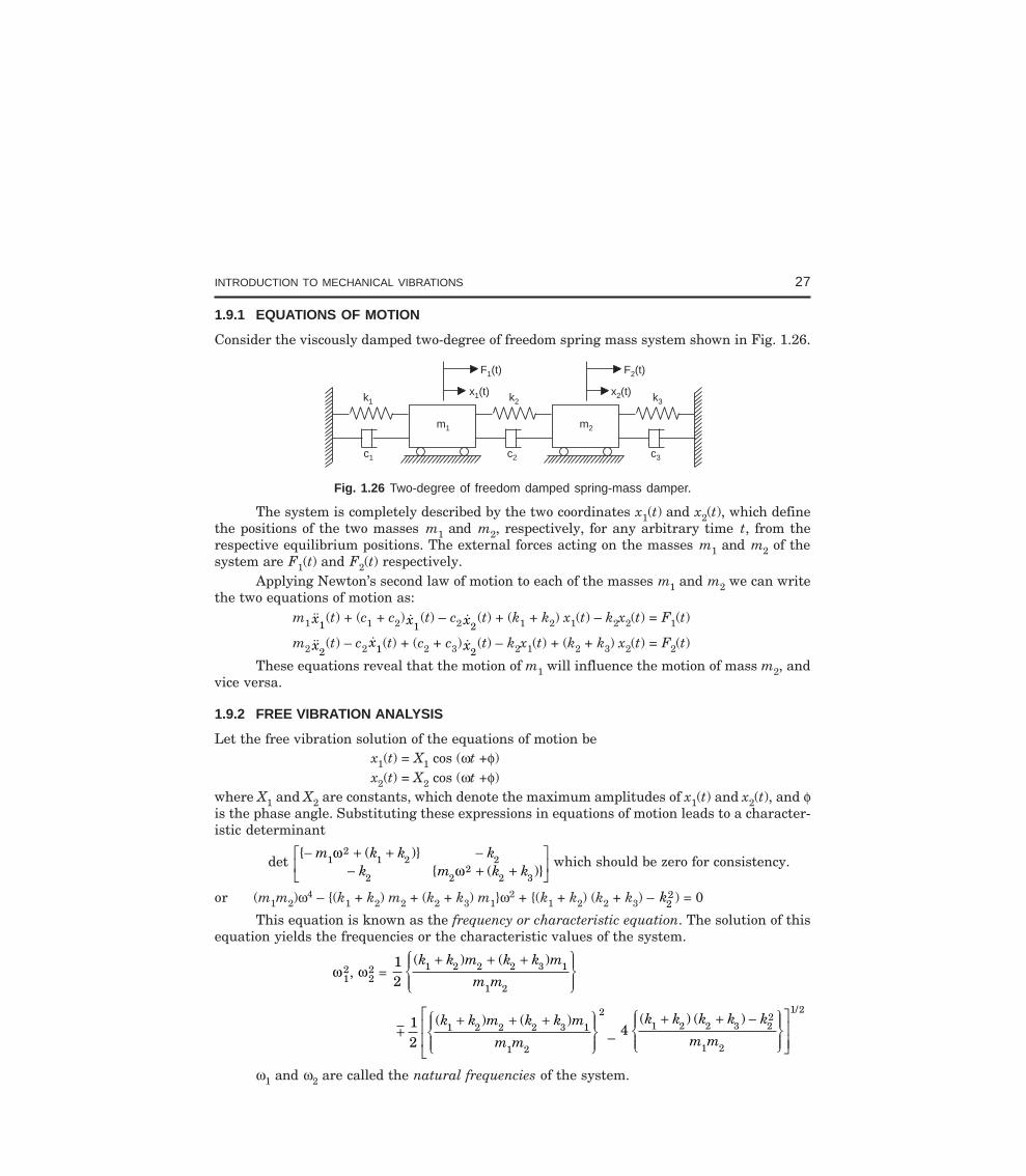
1.9.1 EQUATIONS OF MOTION
Consider the viscously damped two-degree of freedom spring mass system shown in Fig. 1.26.
F (t)1
k1
c3c2c1
k2 k3
m1 m2
F (t)2
x (t)1 x (t)2
Fig. 1.26 Two-degree of freedom damped spring-mass damper.
The system is completely described by the two coordinates x1(t) and x2(t), which definethe positions of the two masses m1 and m2, respectively, for any arbitrary time t, from therespective equilibrium positions. The external forces acting on the masses m1 and m2 of thesystem are F1(t) and F2(t) respectively.
Applying Newton’s second law of motion to each of the masses m1 and m2 we can writethe two equations of motion as:
m1 x1(t) + (c1 + c2) x1
(t) – c2 x2(t) + (k1 + k2) x1(t) – k2x2(t) = F1(t)
m2 x2(t) – c2
x1(t) + (c2 + c3) x2(t) – k2x1(t) + (k2 + k3) x2(t) = F2(t)
These equations reveal that the motion of m1 will influence the motion of mass m2, andvice versa.
1.9.2 FREE VIBRATION ANALYSIS
Let the free vibration solution of the equations of motion bex1(t) = X1 cos (ωt +φ)x2(t) = X2 cos (ωt +φ)
where X1 and X2 are constants, which denote the maximum amplitudes of x1(t) and x2(t), and φis the phase angle. Substituting these expressions in equations of motion leads to a character-istic determinant
det ( )
( )− + + −
− + +LNM
OQP
m k k kk m k k
12
1 2 2
2 22
2 3
ωω
which should be zero for consistency.
or (m1m2)ω4 – (k1 + k2) m2 + (k2 + k3) m1ω
2 + (k1 + k2) (k2 + k3) – k22) = 0
This equation is known as the frequency or characteristic equation. The solution of thisequation yields the frequencies or the characteristic values of the system.
ω12, ω2
2 = 12
1 2 2 2 3 1
1 2
( ) ( )k k m k k m
m m
+ + +RS|T|
UV|W|
++ + +R
S|T|
UV|W|
L
NMM
12
1 2 2 2 3 1
1 2
2( ) ( )k k m k k m
m m – 41 2 2 3 2
2
1 2
1/2( ) ( )k k k k k
m m
+ + −RS|T|
UV|W|OQPP
ω1 and ω2 are called the natural frequencies of the system.
28 SOLVING VIBRATION ANALYSIS PROBLEMS USING MATLAB
The values of X1 and X2 depend on the natural frequencies ω1 and ω2. By denoting the
values of X1 and X2 corresponding to ω1 as X11( ) and X2
1( ) and those corresponding to ω2 as X12( )
and X22( ) :
r1 = X
X
m k k
k
k
m k k21
11
1 12
1 2
2
2
2 12
2 3
( )
( )
( )
( )=
− + +=
− + +ω
ω
r2 = X
X
m k k
k
k
m k k22
12
1 22
1 2
2
2
2 22
2 3
( )
( )
( )
( )=
− + +=
− + +ω
ω
The normal modes of vibration corresponding to ω12 and ω2
2 can be expressed, respec-tively, as
X(1) = X
X
X
r X11
21
11
1 11
( )
( )
( )
( )
RS|T|
UV|W|
=RS|T|
UV|W|
and X(2) = X
X
X
r X12
22
12
2 12
( )
( )
( )
( )
RS|T|
UV|W|
=RS|T|
UV|W|
The vectors X(1) and X(2), which denote the normal modes of vibration, are known asthe modal vectors of the system.
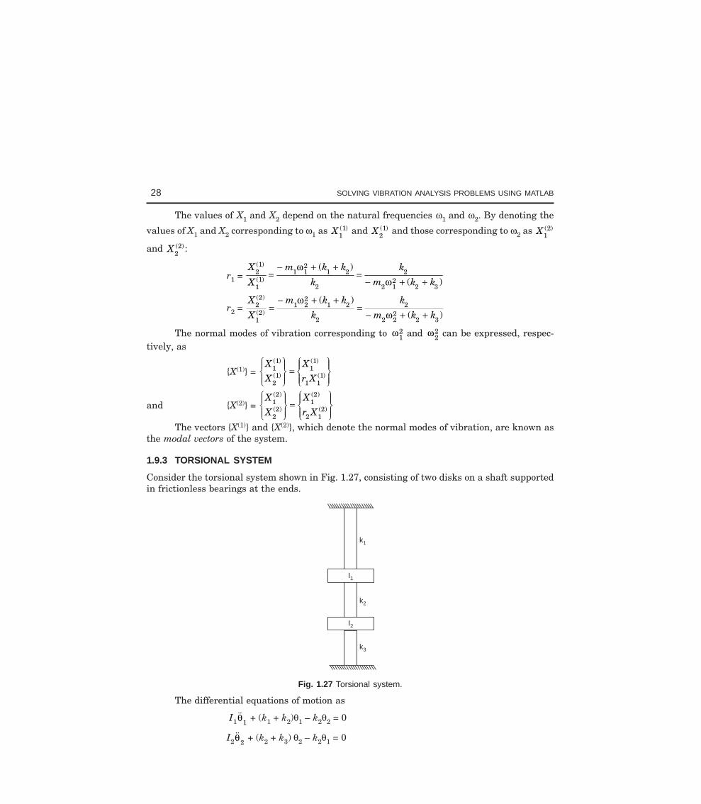
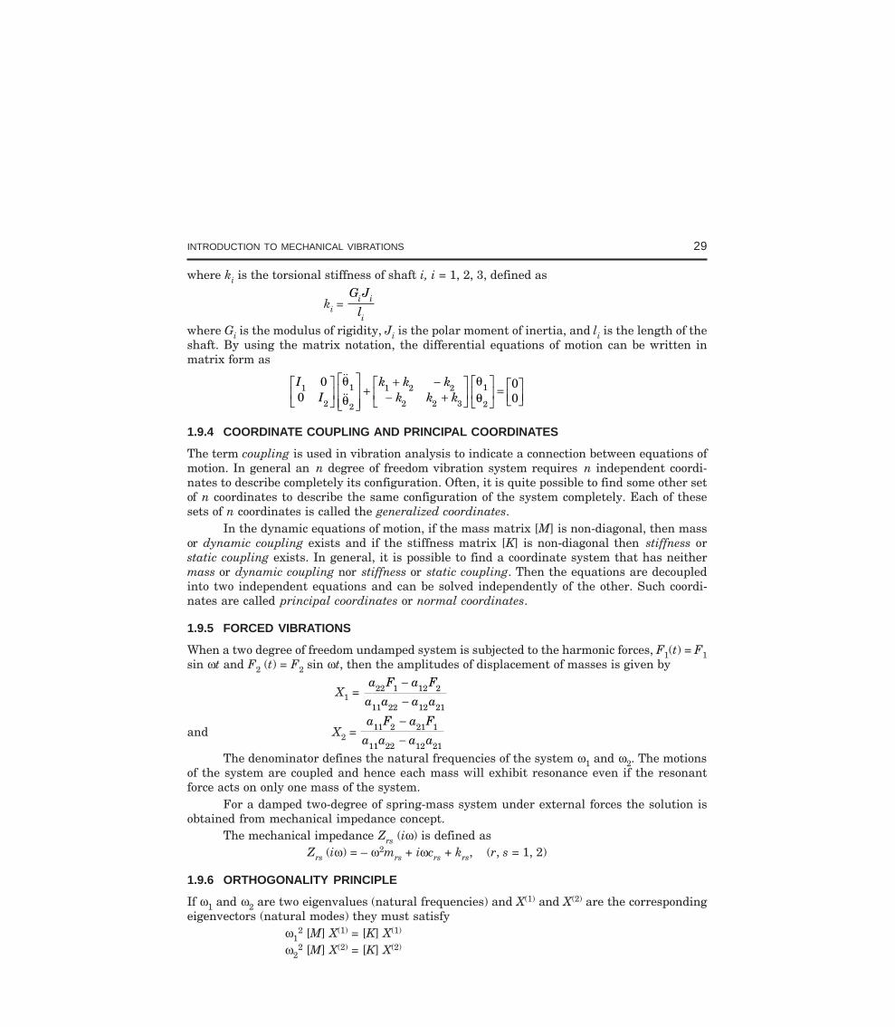
1.9.3 TORSIONAL SYSTEM
Consider the torsional system shown in Fig. 1.27, consisting of two disks on a shaft supportedin frictionless bearings at the ends.
k3
k2
k1
I1
I2
Fig. 1.27 Torsional system.
The differential equations of motion as
I1θ1
+ (k1 + k2)θ1 – k2θ2 = 0
I2θ2 + (k2 + k3) θ2 – k2θ1 = 0
INTRODUCTION TO MECHANICAL VIBRATIONS 29
where ki is the torsional stiffness of shaft i, i = 1, 2, 3, defined as
ki = G J
li i
i
where Gi is the modulus of rigidity, Ji is the polar moment of inertia, and li is the length of theshaft. By using the matrix notation, the differential equations of motion can be written inmatrix form as
II
k k kk k k
1
2
1
2
1 2 2
2 2 3
1
2
00
00
LNM
OQPLNMM
OQPP
++ −
− +LNM
OQPLNM
OQP
= LNMOQP
θθ
θθ
1.9.4 COORDINATE COUPLING AND PRINCIPAL COORDINATES
The term coupling is used in vibration analysis to indicate a connection between equations ofmotion. In general an n degree of freedom vibration system requires n independent coordi-nates to describe completely its configuration. Often, it is quite possible to find some other setof n coordinates to describe the same configuration of the system completely. Each of thesesets of n coordinates is called the generalized coordinates.
In the dynamic equations of motion, if the mass matrix [M] is non-diagonal, then massor dynamic coupling exists and if the stiffness matrix [K] is non-diagonal then stiffness orstatic coupling exists. In general, it is possible to find a coordinate system that has neithermass or dynamic coupling nor stiffness or static coupling. Then the equations are decoupledinto two independent equations and can be solved independently of the other. Such coordi-nates are called principal coordinates or normal coordinates.
1.9.5 FORCED VIBRATIONS
When a two degree of freedom undamped system is subjected to the harmonic forces, F1(t) = F1sin ωt and F2 (t) = F2 sin ωt, then the amplitudes of displacement of masses is given by
X1 = a F a F
a a a a22 1 12 2
11 22 12 21
−−
and X2 = a F a F
a a a a11 2 21 1
11 22 12 21
−−
The denominator defines the natural frequencies of the system ω1 and ω2. The motionsof the system are coupled and hence each mass will exhibit resonance even if the resonantforce acts on only one mass of the system.
For a damped two-degree of spring-mass system under external forces the solution isobtained from mechanical impedance concept.
The mechanical impedance Zrs (iω) is defined asZrs (iω) = – ω2mrs + iωcrs + krs, (r, s = 1, 2)
1.9.6 ORTHOGONALITY PRINCIPLE
If ω1 and ω2 are two eigenvalues (natural frequencies) and X(1) and X(2) are the correspondingeigenvectors (natural modes) they must satisfy
ω12 [M] X(1) = [K] X(1)
ω22 [M] X(2) = [K] X(2)
30 SOLVING VIBRATION ANALYSIS PROBLEMS USING MATLAB
Then it can be shown thatFor ω1 ≠ ω2, [X
(2)]T [M]X(1) = 0This property is very useful, as for example to check the accuracy of computation of
normal modes by its application.
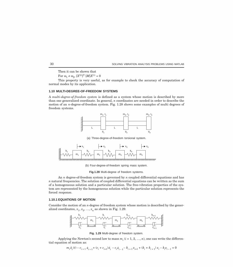
1.10 MULTI-DEGREE-OF-FREEDOM SYSTEMS
A multi-degree-of-freedom system is defined as a system whose motion is described by morethan one generalized coordinate. In general, n coordinates are needed in order to describe themotion of an n-degree-of-freedom system. Fig. 1.28 shows some examples of multi degrees offreedom systems.
L L L
1
m , I1 1 m , I2 2 m , I3 3
2 3
(a) Three-degree-of-freedom torsional system.
k1
x1 x2 x3 x4
k2 k3 k4
m1 m2 m3 m4
(b) Four-degree-of-freedom spring mass system.
Fig.1.28 Multi-degree of freedom systems.
An n degree-of-freedom system is governed by n coupled differential equations and hasn natural frequencies. The solution of coupled differential equations can be written as the sumof a homogeneous solution and a particular solution. The free-vibration properties of the sys-tem are represented by the homogeneous solution while the particular solution represents theforced response.
1.10.1 EQUATIONS OF MOTION
Consider the motion of an n-degree of freedom system whose motion is described by the gener-alized coordinates, x1, x2, …, xn as shown in Fig. 1.29.
c1 ci ci+1 cn+1
m1 m2 mn
k1 ki ki+1 kn+1
Fig. 1.29 Multi-degree of freedom system.
Applying the Newton’s second law to mass mi (i = 1, 2, …, n), one can write the differen-tial equation of motion as:
mi xi (t) – ci + 1 xi + 1+ (ci + ci+1) xi – ci xi − 1
– ki + 1 xi+1 + (ki + ki + 1) xi – kixi – 1 = 0
INTRODUCTION TO MECHANICAL VIBRATIONS 31
For general use, it is convenient to write this equation as in the following matrix form
[M] x(t) + [C] x(t) + [K]x(t) = 0with [M], [C] and [K] being square matrices containing the coefficients mij, cij and kij respec-tively.
In this particular case, the mass-matrix is diagonal. For a different set of coordinates,[M] is not necessarily diagonal.
1.10.2 STIFFNESS INFLUENCE COEFFICIENTS
For a linear system, inertial, damping and stiffness properties enter explicitly in the differen-tial equations through the mass-coefficients mij, damping-coefficients cij and stiffness coeffi-cients kij (i, j = 1,2,…, n) respectively. Of the three, stiffness coefficients are the elastic proper-ties causing a dynamic system to vibrate, e.g., restoring-forces. Stiffness coefficients are alsoknown as stiffness influence coefficients. Stiffness influence coefficients kij is defined as theforce required at x = xi to produce a unit displacement uj = 1 at point x = xj and also thedisplacements at all other points for which x ≠ xj are zero. In other words, they define a rela-tion between the displacement at a point and the forces acting at various other points of sys-tem. Invoking the superposition principle, the force at x = xi producing displacements uj atx = xj (j =1,2,…, n) is
Fi = j
n
ij jk u=
∑1
1.10.3 FLEXIBILITY INFLUENCE COEFFICIENTS
Let the system be acted upon by a single-force Fj at x = xj and consider the displacement of anyarbitrary point x = xi (i = 1, 2, …, n) due to force Fj. Flexibility influence coefficient is defined asthe displacement of the point x = xi due to unit force Fj = 1 applied at the point x = xj. Invokingthe principle of superposition and obtaining displacement ui at x = xi resulting from all forcesFj (j = 1, 2, …, n) by simply summing up the individual contributions
Ui = j
n
ij ja F=
∑1
Note that the units of aij are m/N.For a single-degree of freedom system with only one spring, the stiffness influence
coefficient is merely the spring-constant, whereas the flexibility influence coefficient is itsreciprocal.
1.10.4 MATRIX FORMULATION
For multi-degree of freedom systems, a more general formulation is employed. Arranging theflexibility and stiffness influence coefficients in the square matrices as
[aij] = [A], and [kij] = [K]where [A] is the flexibility matrix and [K] is the stiffness matrix.
The flexibility and stiffness matrices are the inverse of one another. Often the stiffnesscoefficients are easier to evaluate than the flexibility coefficients. When the stiffness matrix issingular, the flexibility matrix does not exist. This implies that the system admits rigid-bodymotions, in which the system undergoes no elastic deformations. This can happen when supports
32 SOLVING VIBRATION ANALYSIS PROBLEMS USING MATLAB
do not fully restrain the system from moving. Thus in the absence of adequate supports, thedefinition of flexibility coefficients cannot be applied, so that the coefficients are not defined.
1.10.5 INERTIA INFLUENCE COEFFICIENTS
The mass-matrix is associated with the kinetic energy. For a multi-degree of freedom system
with xi as the velocity of mass mi (i = 1, 2, …, n.), the kinetic energy is given by
T = 12
[ ] x M xT
where [M] is the mass-matrix or inertia matrix.The elements of the mass-matrix mij are known as the inertia influence coefficients. The
coefficients mij can be obtained using the impulse-momentum relations. The inertia influencecoefficients m1j, m2j, …, mnj are defined as the set of impulses applied at points 1, 2, …, nrespectively, to produce a unit velocity at points 1, 2, …, n respectively, to produce a unitvelocity at point j and zero velocity at every other point. Thus, for a multi degree of freedomsystem, the total impulse at point i, can be found by summing up the impulses causing the
velocities x j (j = 1, 2, …, n) as
~F = [M] X
where [M] is the mass matrix, X and ~F are the velocity and impulse vectors of size
n × 1 respectively.
1.10.6 NORMAL MODE SOLUTION
The general formulation of the differential equations governing the free-vibrations of a linear-undamped n-degree-of-freedom system can be written as
[M] x + [K]x = 0where [M] and [K] are symmetric n × n mass and stiffness matrices respectively and x is the n-dimensional column-vector of generalized coordinates.
Free vibrations of a multi-degree-of-freedom system are initiated by the presence of aninitial potential or kinetic energy.
The normal-mode solution in the form ofx(t) = Xeiωt
where ω the frequency of vibration and X is an n-dimensional vector called a mode shape. Eachnatural frequency has at least one corresponding mode shape. The general solution is a linearsuperposition over all possible modes.
The frequency or eigenvalue equation is defined as– ω2 [M]X + [K]X = 0
The trivial solution (X = 0) is obtained unlessdet[[M]–1 [K] – ω2I] = 0
Thus ω2 must be an eigenvalue of [M]–1 [K]. This form is called characteristic equation.The square of a real positive eigenvalue has two possible values, one positive and one negative.While both are used to develop the general solution, the positive square root is identified as anatural frequency. The mode shape is the corresponding eigenvector.
INTRODUCTION TO MECHANICAL VIBRATIONS 33
1.10.7 NATURAL FREQUENCIES AND MODE SHAPES
Generally in vibration problems, the characteristic equation has only real-roots since thematrices under consideration are symmetric. Assuming that all the eigenvalues of [M]–1 [K]corresponding to the symmetric mass and stiffness matrices are non-negative. Then thereexist n-real natural frequencies that can be arranged by ω1 ≤ ω2 ≤ … ωn. Each distinct eigenvalueω i
2, i = 1, 2, …, n, has a corresponding non-trivial eigenvector Xi, which satisfies
[M]–1[K]Xi = ω i2Xi
This mode shape Xi is an n-dimensional column vector of the form
Xi =
XX
X
i
i
in
1
2
L
N
MMMM
O
Q
PPPP
This mode shape is not unique. The eigenvector is unique only to arbitrary multiplica-tive constant. Normalization schemes exist such that the constant is chosen so the eigenvectorsatisfies an externally imposed condition. The algebraic complexity of the solution growsexponentially with the number of degrees of freedom. Hence, numerical methods, which do notrequire the evaluation of the characteristic equation, are used for systems with a large numberof degrees of freedom.
1.10.8 MODE SHAPE ORTHOGONALITY
In the solution of problems involving multi-degree-of-freedom vibration, one useful fundamen-tal relation exists between the principal modes. Consider any two principal modes of oscilla-tion of a system of several degrees of freedom. Let these be rth and sth modes and the corre-
sponding eigenvalues be ω r2 and ω s
2, then it can shown that
X rT [M]Xs = 0, r ≠ s
X rT [K]Xs = 0 r ≠ s
These define the matrix form of the orthogonal relationships between principal modesof vibration. Since [M] is often a diagonal matrix and [K] is not, it is usually simpler to writethe orthogonality matrix with respect to [M]. The orthogonality relation with respect to [M] iswritten in expanded form as
i
n
j
n
ij ir
jsm x x
= =∑ ∑
1 1
= 0, r ≠ s
Thus the orthogonality relation for the principal modes of vibration is essentially a rela-tion between the amplitudes of two principal modes. These are not necessarily successive modesbut any two modes. It is convenient to normalize mode shapes by requiring that the kineticenergy scalar product of a mode shape with itself is equal to one.
1.10.9 RESPONSE OF A SYSTEM TO INITIAL CONDITIONS
Response of multi-degree-of-freedom system subjected to initial excitations x(0) and x(0) inthe general form can be written as
34 SOLVING VIBRATION ANALYSIS PROBLEMS USING MATLAB
x(t) = r
n
rT
rr
rT
r rU Mx t U Mx t U=
∑ +LNMM
OQPP1
01
0( ) cos ( ) sinωω
ω
Here each of the natural modes can be excited independently of the other.
In the equations of free motion including viscous damping, we can assume a harmonic form forthe response. Due to the presence of damping, the characteristic equation will be a polynomialthat has complex conjugate roots. For a given complex conjugate eigenvalues there are conju-gate eigenvectors. The normal mode method or modal analysis applies only to undamped sys-tems or systems where the damping can be made mathematically equivalent to the mass orstiffness matrix. Sometimes damping can be ignored in the forced response of a vibratingsystem.
For some special systems, where the damping matrix is linearly related to the mass and stiff-ness matrices, the simultaneous diagonalization of the stiffness and mass matrices can beaccomplished along with that of the damping matrix. Such systems are called proportionaldamping systems.
Here [C] = α[K] + β[M]where α and β are constants.
Differential equations governing the free vibrations of a linear system with propor-tional damping can be written as
[M] X + (α[K] + β[M]) X + [K] X = 0If ω1 ≤ ω2 ≤ … ωn are the natural frequencies of an undamped system whose mass-
matrix is [M] and stiffness matrix [K] and U1, U2, … Un are the corresponding normalizedmode shapes. The expansion-theorem implies that X can be written as a linear combination ofthe mode shape vector.
X = Σpi Ui
The matrix triple products possessing orgthogonality properties, is written as
[U]T[M][U] P + [U]T (α[K] + β[M]) [U] P + [U]T[K][U]P = 0The orthogonality of modes with respect to mass and stiffness permits the following
substitutions:[U]T [M] [U] = [I]
and [U]T [K] [U] = [diag ω2] = [Ω]The equations can now be decoupled into governing equations for each degree of free-
dom. Mathematically,
( ) p p pi i i i i+ + +αω β ω2 2 = 0
In this connection, modal damping ratio is defined as ξi = 12
αωβ
ωii
+FHG
IKJ
INTRODUCTION TO MECHANICAL VIBRATIONS 35
The general solution for free vibration problem under ξi < 1 is given by
pi(t) = Aie ti iti i i
− − −ξ ω ω ξ φsin ( )1 2
where Ai and φi are constants determined from the initial conditions. Finally the solution isobtained in terms of generalized coordinates.
The differential equations governing the free-vibrations of a multi-degree-of-freedom systemwith viscous damping are given by
[M] X + [C] X + [K] X = 0If the damping is arbitrary, then the principal coordinates of the undamped system do
not uncouple the above equation. The equation can be reformulated as 2n first-order differen-tial equations by writing
[~
] [~
]M y K y+ = 0
where [~
] [ ][ ] [ ]
M O MM C
= LNM
OQP , [
~] [ ]
[ ]K M O
O K= −LNM
OQP, y =
XXLNM
OQP
If the values of γ are complex-conjugate eigenvalues of [~
] [~
]M K−1 and φ is a correspond-ing eigenvector, then the solution takes the form as
y = φ e–γt
Differential equations governing the motion of an n-degree of freedom undamped system sub-ject to a single-frequency excitation with all excitation terms at the same phase can be writtenas:
[M] x + [K]x = F sin ωtwhere F is an n-dimensional vector of constant forces. A particular solution of the form isassumed as follows:
x(t) = U sin ωtwhere U is an n-dimensional vector of undetermined coefficients.
It results in by usual method as a solutionU = (–ω2 [M] + iω[C] + [K])–1 F
Alternative to this method of undetermined coefficients, Laplace transform method canalso be employed.
The differential equations governing the forced vibration motion of an undamped linear n-degree-of-freedom system are
M X + KX = F
36 SOLVING VIBRATION ANALYSIS PROBLEMS USING MATLAB
The method of modal analysis uses the principal coordinates of the system to uncouplethis equation as follows:
i
n
i j ii
n
i j i jp X MX p X KX X F= =∑ ∑+ =
1 1
( ) ( )
Application of mode shape orthogonality leads to only one non-zero term in each sum-mation, i.e., the term corresponding to i = j. Since the mode shapes are normalized, the follow-ing set of equations are obtained
( )p p g tj j j j+ =ω2
where gj(t) = Xj FIf the initial conditions for pi are both zero, then the convolution integral solution is
given by
pi(t) = 1
0ωτ ω τ τ
i
t
i ig t dz −( ) sin [ ( )]
Once the solution for each pi is obtained, the original generalized coordinates can bedetermined.
The same methodology can be applied to systems having proportional damping.Here it leads to the differential equations for the principal coordinates as
( )p p p g ti i i i i i i+ + =2 2ξ ω ωwhere ξi is modal damping-ratio.
In this case, the convolution-integral solution is given by
pi(t) = 1
0ωτ ω τ τξ ω τ
d
t
it
d
i
i i
ig e t dz − − −( ) sin ( )( )
where1
ωdi
= ωi 1 2− ξ i
There are two general approaches to classical dynamics: vectorial dynamics and analyticaldynamics. Vectorial dynamics is based directly on the application of Newton’s second law ofmotion, concentrating on forces and motions. Analytical dynamics treats the system as a wholedealing with scalar quantities such as the kinetic and potential energies of the system. Lagrangeproposed an approach, which provides a powerful and versatile method for the formulation ofthe equations of motion for any dynamical system. Lagrange’s equation obtains the equation ofmotion in generalized coordinates approaching the system from the analytical dynamics pointof view. Lagrange’s equations are differential equations in which one considers the energies ofthe system and the work done instantaneously in time.
1.16.1 GENERALIZED COORDINATES
The coordinates used to describe the motion in each degree of freedom of a system are termedas generalized coordinates. They may be Cartesian, polar, cylindrical or spherical coordinates,provided any one of them can be used to describe the configuration of the system where the
INTRODUCTION TO MECHANICAL VIBRATIONS 37
motion along any one coordinate direction is independent of others. But, sometimes they maynot have such simple physical or geometrical meaning. For example, the deflections of a string,stretched between two points, can be expressed in the form of trigonometric Fourier series,and the coefficients of all the terms in the series can be considered as a generalized coordinateset. This is because each trigonometric function in the series may be considered as a uniquedegree of freedom and the coefficients describe the extent of deflection in each degree of free-dom.
It is possible to transform the coordinates from any one system to the generalizedcoordinate system or vice versa, through coordinate transformation. Consider a mechanicalsystem consisting of N particles whose positions are (xi, yi, zi), i = 1,2,…, N, in a Cartesiancoordinate system. The motion of the mechanical system is completely defined if the variationwith time of these positions i.e. xi = xi(t), yi = yi(t), zi = zi(t), are known. These 3N coordinatescompletely define a representative space. If it is possible to find another set of generalizedcoordinates, qi, i = 1,2,….n, where n = 3N, then these two coordinate systems are related by thefollowing:
xi(t) = xi(q1, q2, …, qn, t)yi(t) = yi(q1, q2, …, qn, t)zi(t) = zi(q1, q2, …, qn, t)
!"
The principle of virtual work is essentially a statement of the static or dynamic equilibrium ofa mechanical system. A virtual displacement, denoted by δr, is an imaginary displacement andit occurs without the passage of time. The virtual displacement being infinitesimal obeys therules of differential calculus.
Consider a mechanical system with N particles in a three-dimensional space whosecartesian coordinates are (x1, y1, z1,…,zn). Suppose the system is subject to k constraints φj (x1,y1, z1,…,zn, t) = 0, j = 1,2,…,k. The virtual displacements δx1,δy1, δz1 etc. are said to be consist-ent with the system constraints if the constraint equations are still satisfied.
The virtual work performed by the resultant force vector Fi over the virtual displace-
ment vector δri of particle i is
δW = F ri ii
N
. δ=∑
1
When the system is in equilibrium, the resultant force acting on each particle is zero.The resultant force is the sum of the applied force and the reaction force or the constraintforce. The virtual work done by all the forces in moving through an arbitrary virtual displace-ment consistent with the constraints is zero.
#
The principle of virtual work is extended to dynamics, in which form it is known as D’ Alembert’sprinciple. The principle of virtual work is extended to the dynamic case by considering theinertia forces and considering the systems to be in dynamic equilibrium.
38 SOLVING VIBRATION ANALYSIS PROBLEMS USING MATLAB
The generalized principle of D’Alembert states that the virtual work performed by theeffective forces through infinitesimal virtual displacements compatible with the system con-straints is zero.
$
If Qi is called the generalized force in the direction of the ith generalized coordinate, T is thekinetic energy and V is potential energy, then Lagrange’s equation is given by
ddt
Tq
Tq
Vqi i i
∂∂
∂∂
∂∂
FHG
IKJ
− + = Qi
Expressing T – V = L, called the Lagrangian, the equation can be written as
ddt
Lq
Lq
Qi i
i
∂∂
∂∂
FHG
IKJ
− =
%
An alternative approach to the study of motion is the use of variational principle, which viewsthe motion as a whole from the beginning to the end. This involves a search for the path in theconfiguration space, which yields a stationary value for a certain integral. Unlike as in thecase of differential equations, the initial and final points in the configuration space are fixed inthis approach. The most celebrated variational principle in dynamics is the Hamilton’s principle.
Hamilton’s principle is the most important and powerful variational principle in dynamics. Itis derived from the generalized D’Alembert’s principle. The generalized version of Hamilton’sprinciple can be written as
t
tT W dt
0
10z + =( )δ δ or
t
tT V dt
0
10z − =δ ( ) , δ
t
tL dt
0
10z =
where L = T – V.The usual form of Hamilton’s principle applies to a more restricted class of systems,
which are called conservative systems. In these systems all the applied forces are derivablefrom a potential function V(q, t).
The usual form of Hamilton’s principle states that: The actual path in the configurationspace followed by a holonomic system from t0 and t1 is such that the integral
I =t
tL dt
0
1zis stationary with respect to any path variations, which vanish at the end points.
INTRODUCTION TO MECHANICAL VIBRATIONS 39
Benaroya, H., Mechanical Vibrations, Prentice Hall, Upper Saddle River, NJ, 1998.Bhat, R.B., and Dukkipati, R.V., Advanced Dynamics, Narosa Publishing House, New
Delhi, India, 2001.Dimarogonas, A.D., and Haddad, S.D., Vibration for Engineers, Prentice Hall,
Englewood cliffs, NJ, 1992.Dukkipati, R.V., Advanced Engineering Analysis, Narosa Publishing House, New Delhi,
India, 2006.Dukkipati, R.V., Advanced Mechanical Vibrations, Narosa Publishing House, New
Delhi, India, 2006.Dukkipati, R.V., and Amyot, J.R., Computer Aided Simulation in Railway Vehicle
Dynamics, Marcel-Dekker, New York, NY, 1988.Dukkipati, R.V., and Srinivas, J., A Text Book of Mechanical Vibrations, Prentice
Hall of India, New Delhi, India, 2005.Dukkipati, R.V., and Srinivas, J., Vibrations: Problem Solving Companion, Narosa
Publishing House, New Delhi, India, 2006.Dukkipati, R.V., Vehicle Dynamics, Narosa Publishing House, New Delhi, India, 2000.Dukkipati, R.V., Vibration Analysis, Narosa Publishing House, New Delhi, India, 2005.Garg, V.K., and Dukkipati, R.V., Dynamics of Railway Vehicle Systems, Academic
Press, New York, NY, 1984.Kelly, S.G., Fundamentals of Mechanical Vibration, McGraw Hill, New York, NY, 1993.Meirovitch, L., Elements of Vibration Analysis, 2nd ed., McGraw Hill, New York, NY,
1986.Newland, D.E., Mechanical Vibration Analysis and Computation, Longman, 1989.Ramamurti, V., Mechanical Vibration Practice With Basic Theory, CRC Press, Boca
Raton, FL, 2000.Rao, J.S., and Gupta, K., Introductory Course on Theory and Practice of Mechanical
Vibrations, Wiley Eastern, New Delhi, India, 1984.Rao, S.S., Mechanical Vibrations, 3rd ed., Addison Wesley, Reading, MA, 1995.Seto, W.W., Theory and Problems of Mechanical Vibrations, Schaum series, McGraw
Hill, New York, NY, 1964.Srinivasan, P., Mechanical Vibration Analysis, Tata McGraw Hill, New Delhi, India,
1982.Steidel, R.F., An Introduction to Mechanical Vibrations, 3rd ed., Wiley, New York, NY,
1981.Thomson, W.T., and Dahleh, M.D., Theory of Vibrations with Applications, 5th ed.,
Prentice Hall, Englewood Cliffs, NJ, 199.Timoshenko, S., Young, D.H., and Weaver, W., Vibration Problems in Engineering,
5th ed., Wiley, New York, NY 1990.Tong, K.N., Theory of Mechanical Vibration, Wiley, New York, NY, 1960.Tse, F.S., Morse, I.E., and Hinkle, R.T., Mechanical Vibrations, Allyn and Bacon,
Boston, MA, 1963.Vierck, R.K., Vibration Analysis, 2nd ed., Harper & Row, New York, NY, 1979.
40 SOLVING VIBRATION ANALYSIS PROBLEMS USING MATLAB
Terminology used frequently in the field of vibration analysis is compiled here from varioussources including from the document prepared by ISO, TCO-108, Mechanical Vibration andShock, American National Standards Institute Inc., New York.
Acceleration: Acceleration is a vector quantity that specifies the time rate of change ofvelocity.
Amplification Factor: See magnification ratio.Amplification: The amount of power or amplitude in an electric signal. Devices such
as transistors are used to create or increase amplification.Amplitude Ratio: Amplitude ratio or magnifications factor is the ratio of the maxi-
mum force developed in the spring of a mass-spring-dashpot system to the maximum value ofthe exciting force.
Amplitude: Amplitude is the maximum distance from either side of the natural posi-tion that the object can travel once the object is released.
Analytical Dynamics: See analytical mechanics.Analytical Mechanics: Analytical mechanics or variational approach to mechanics or
analytical dynamics, considers the system as a whole, rather that the individual componentsseparately, a process that excludes the reaction and constraint forces automatically.
Angular Frequency (Circular Frequency): The angular frequency of a periodic quan-tity, in radians per unit time, is the frequency multiplied by 2π.
Angular Impulse: The angular impulse of a constant torque T acting for a time t is theproduct Tt.
Angular Mechanical Impedance (Rotational Mechanical Impedance): Angularmechanical impedance is the impedance involving the ratio of torque to angular velocity. (SeeImpedance.)
Angular Momentum: The angular momentum of a body about its axis of rotation isthe moment of its linear momentum about the axis.
Angular Motion: See rotational particle motion.Anti-resonance: For a system in forced oscillation, anti-resonance exists at a point
when any change, however small, in the frequency of excitation causes an increase in theresponse at this point.
Auxiliary Mass Damper (Damped Vibration Absorber): An auxiliary mass damperis a system consisting of a mass, spring, and damper which tends to reduce vibration by thedissipation of energy in the damper as a result of relative motion between the mass and thestructure to which the damper is attached.
Balancing: Balancing is a procedure for adjusting the mass distribution of a rotor sothat vibration of the journals, or the forces on the bearings at once-per-revolution, are reducedor controlled.
Basic Law of Nature: A basic law of nature is a physical law that applies to all physicalsystems regardless of the motional from which the system is constructed.
Beats: Beats are periodic variations that result from the superposition of two simpleharmonic quantities of different frequencies fl and f2. They involve the periodic increase anddecrease of amplitude at the beat frequency.
INTRODUCTION TO MECHANICAL VIBRATIONS 41
Centrifugal Force: If a body rotates at the end of an arm, the force is provided by thetension in the arm. The reaction to this force acts at the centre of rotation and is called thecentrifugal force. It represents the inertia force of the body, resisting the change in the directionof its motion.
Centripetal Acceleration: The acceleration that is directed towards the centre ofrotation is called the centripetal acceleration.
Centripetal Force: A centre seeking force that causes an object to move towards thecentre.
Circular Frequency: See Angular Frequency.Circular Motion: See rotational particle motion.Complex Function: A complex function is a function having real and imaginary parts.Complex Vibration: Complex vibration is vibration whose components are sinusoids
not harmonically related to one another. See Harmonic.Compliance: Compliance is the reciprocal of stiffness.Conservation of Angular Momentum: The total angular momentum of a system of
masses about any one axis remains constant unless acted upon by an external torque aboutthat axis.
Conservation of Energy: Energy can neither be created nor destroyed.Conservation of Linear Momentum: The total momentum of a system of masses in
any one direction remains constant unless acted upon by an external force in that direction.Conservative System: In a conservative system, there is no mechanism for dissipat-
ing or adding energy.Continuous Assumption: The continuous assumption implies that a system can be
treated as a continuous piece of matter.Continuous System: A system with an infinite number of degrees of freedom is called
a continuous system or distributed parameter system.Coulomb Damping: Coulomb damping is the damping that occurs due to dry friction
when two surfaces slide against one another.Coupled Modes: Coupled modes are modes of vibration that are not independent but
which influence one another because of energy transfer from one mode to the other. (See modeof vibration.)
Coupling Factor, Electromechanical: The electromechanical coupling factor is a factorused to characterize the extent to which the electrical characteristics of a transducer are modi-fied by a coupled mechanical system, and vice versa.
Coupling: Coupling is the term used in mechanical vibration to indicate a connectionbetween equations of motion.
Critical Damping: Critical damping is the minimum viscous damping that will allow adisplaced system to return to its initial position without oscillation.
Critical Speed: Critical speed is a speed of a rotating system that corresponds to aresonant frequency of the system.
Critical Velocity: The minimum velocity at the highest point of the loop in order tocomplete a cycle is called the critical velocity.
Critically Damped System: The system is said to be critically damped if the amountof damping is such that the resulting motion is on the border between the two cases ofunderdamped and over damped systems.
42 SOLVING VIBRATION ANALYSIS PROBLEMS USING MATLAB
Cycle: A cycle is the complete sequence of values of a periodic quantity that occur dur-ing a period.
D’Alembert’s Principle: The virtual performed by the effective forces through infini-tesimal virtual displacements compatible with the system constraints is zero.
Damped Natural Frequency: The damped natural frequency is the frequency of freevibration of a damped linear system. The free vibration of a damped system may be consideredperiodic in the limited sense that the time interval between zero crossings in the same direc-tion is constant, even though successive amplitudes decrease progressively. The frequency ofthe vibration is the reciprocal of this time interval.
Damping Ratio: The damping ratio is defined as the ratio of the actual value of thedamping to the critical damping coefficient.
Damping: The process of energy dissipation is generally referred to in the study ofvibrations as damping.
Degrees-of-freedom: The number of degrees-of-freedom of a mechanical system is equalto the minimum number of independent coordinates required to define completely the posi-tions of all parts of the system at any instant of time. In general, it is equal to the number ofindependent displacements that are possible.
Dependent Variables: Dependent variables are the variables that describe the physi-cal behaviour of the system.
Deterministic Excitation: If the excitation force is known at all instants of time, theexcitation is said to be deterministic.
Discrete System: A system with a finite number of degrees of freedom is a discretesystem.
Displacement: Displacement (or linear displacement) is the net change in a particle’sposition as determined from the position function.
Displacement: Displacement is a vector quantity that specifies the change of positionof a body or particle and is usually measured from the mean position or position of rest. Ingeneral, it can be represented as a rotation vector or a translation vector, or both.
Distributed Parameter System: See continuous system.Distributed Systems: Systems where mass and elasticity are considered to be distrib-
uted parameters are called distributed systems.Driving Point Impedance: Driving point impedance is the impedance involving the
ratio of force to velocity when both the force and velocity are measured at the same point andin the same direction. (See Impedance.)
Dry Friction Damping: (See Coulomb Damping.)Duration of Shock Pulse: The duration of a shock pulse is the time required for the
acceleration of the pulse to rise from some stated fraction of the maximum amplitude and todecay to this value. (See Shock Pulse.)
Dynamic Vibration Absorber (Tuned Damper): A dynamic vibration absorber is anauxiliary mass-spring system, which tends to neutralize vibration of a structure to which it isattached. The basic principle of operation is vibration out-of-phase with the vibration of suchstructure, thereby applying a counteracting force.
Dynamically Coupled: If an equation contains cross products of velocity, or if thekinetic energy contains cross products of velocity, that equation of motion is dynamically coupled.
Dynamics: Dynamics is the study of moving objects.
INTRODUCTION TO MECHANICAL VIBRATIONS 43
Elasticity: A material property that causes it to return to its natural state after beingcompressed.
Energy: Energy is the capacity to do work, mechanical energy being equal to the workdone on a body in altering either its position or its velocity.
Environment: (See Natural Environments and Induced Environment.)Equivalent System: An equivalent system is one that may be substituted for another
system for the purpose of analysis. Many types of equivalence are common in vibration andshock technology: (1) equivalent stiffness; (2) equivalent damping; (3) torsional system equiva-lent to a translational system; (4) electrical or acoustical system equivalent to a mechanicalsystem; etc.
Equivalent Viscous Damping: Equivalent viscous damping is a value of viscous damp-ing assumed for the purpose of analysis of a vibratory motion, such that the dissipation ofenergy per cycle at resonance is the same for either the assumed or actual damping force.
Excitation (Stimulus): Excitation is an external force (or other input) applied to asystem that causes the system to respond in some way.
External forces: Actions of other bodies on a rigid body are known as external forces.Flexibility Matrix: The flexibility matrix is the inverse of the stiffness matrix.Force: Force is a push or a pull that one body exerts on another, includes gravitational,
electrostatic, magnetic and contact influences.Forced Vibrations: Vibrations, which occurs in the presence of an external excitation,
are called forced vibrations.Foundation (Support): A foundation is a structure that supports the gravity load of a
mechanical system. It may be fixed in space, or it may undergo a motion that provides excita-tion for the supported system.
Fraction of Critical Damping: The fraction of critical damping (damping ratio) for asystem with viscous damping is the ratio of actual damping coefficient c to the critical damp-ing coefficient cc.
Free Body Diagram Method: One method of deriving the differentiated equations ofmotion, referred to as the free body diagram method, involves applying conservation laws tofree body diagrams of the system drawn at an arbitrary instant.
Free Vibrations: A system is undergoing free vibrations when the vibrations occur inthe absence of an external excitation.
Frequency, Angular: (See Angular Frequency.)Frequency: The frequency is the number of cycles the system executes in a period of
time and is the reciprocal of the period.Friction: Friction is a force that always resists motion or impending motion.Fundamental Frequency: The natural frequencies can be arranged in order of in-
creasing magnitude and the lowest frequency is referred to as the fundamental frequency.Fundamental Mode of Vibration: The fundamental mode of vibration of a system is
the mode having the lowest natural frequency.Generalized Coordinates: A set of independent coordinates which properly and com-
pletely defines the configuration of a system and whose number is equal to the number ofdegrees of freedom is called the generalized coordinates.
Generalized Forces: The generalized forces are not usually actual or observable forcesacting on the system, but some component of a combination of such forces.
44 SOLVING VIBRATION ANALYSIS PROBLEMS USING MATLAB
Gravity Acceleration: Gravity is measured in terms of the acceleration a planet givesto an object on Earth. The value of gravity acceleration is 9.8 m/sec2.
Grid Points: See Mesh Points.Harmonic Excitations: If the excitation force is periodic the excitations is said to be
harmonic.Harmonic Motion: (See Simple Harmonic Motion.)Harmonic Response: Harmonic response is the periodic response of a vibrating sys-
tem exhibiting the characteristics of resonance at a frequency that is a multiple of the excita-tion frequency.
Harmonic: A harmonic is a sinusoidal quantity having a frequency that is an integralmultiple of the frequency of a periodic quantity to which it is related.
Holonomic Coordinates: If each of the coordinates is independent of the others, thecoordinates are known as holonomic coordinates.
Holonomic System: Systems having equations of constraint containing only coordi-nates or coordinates and time are called holonomic systems.
Homogenous Differential Equation: A differential equation in which all terms con-tain the unknown function or its derivative is known as a homogenous differentiated equation.
Hysteric Damping: The existence of hysterics loop leads to energy dissipation fromthe system during each cycle, which causes natural damping called hysterics damping.
Impact: An impact is a single collision of one mass in motion with a second mass, whichmay be either in motion or at rest.
Impedance: Mechanical impedance is the ratio of a force-like quantity to a velocity-like quantity when the arguments of the real (or imaginary) parts of the quantities increaselinearly with time. Examples of force-like quantities are: force, sound pressure, voltage, andtemperature. Examples of velocity-like quantities are: velocity, volume velocity, current, andheat flow. Impedance is the reciprocal of mobility.
Impulse: Impulse is the product of a force and the time during which the force is ap-plied; more specifically, the impulse is Fdt where the force F is time dependent and equal tozero before time t1 and after time t2.
Impulsive Force: An impulsive force is defined as a force which has a large magnitudeand acts during a very short time duration such that the time integral of the force is finite.
Impulsive Torque: A torque, which acts for a very short time, is referred to as animpulsive torque.
Independent Variables: Independent variables are the variables with which thedependent variable changes.
Influence Coefficient: An influence coefficient, denoted by ∝12, is defined as the sta-tus deflection of the system at position 1 due to a unit force applied at position 2 when the unitforce is the only force acting.
Internal Forces: Internal forces hold together parts of a rigid body.Isolation: Isolation is a reduction in the capacity of a system to respond to an excita-
tion, attained by the use of a resilient support. In steady-state forced vibration, isolation isexpressed quantitatively as the complement of transmissibility.
Jerk: Jerk is a vector that specifies the time rate of change of acceleration; jerk is thethird derivative of displacement with respect to time.
INTRODUCTION TO MECHANICAL VIBRATIONS 45
Kinematics: Kinematics is the study of a body’s motion independent of the force on thebody. It is a study of the geometry of motion without consideration of the causes of motion.
Kinematics: The branch of mechanics that studies the motion of objects without refer-ence to the forces that causes the motion.
Kinetic Coefficient of Friction: Coulombs law states that the friction force is propor-tional to the normal force developed between the mass and the surface. The constant of pro-portions µ is called the kinetic coefficient of friction.
Kinetic Energy: The kinetic energy of a body is the energy it possesses due to itsvelocity. If a body of mass m attains a velocity v from rest under the influence of a force P andmoves a distance s, then, work done by P is Ps and the kinetic energy of the body is [1/2 mv2].
Kinetics: Kinetics is the study of motion and the forces that cause motion.Lagrange’s Method: The technique known as Lagrange’s method utilizes both the
principle of virtual displacements and D’Alembert principle to derive the equations of motionof a vibrating system.
Lagrangian Function: See Lagrangian.Lagrangian or Lagrangian Function: The Lagrangian or the Lagrangian function is
defined as the difference between the kinetic energy and the potential energy of a system.Line Spectrum: A line spectrum is a spectrum whose components occur at a number of
discrete frequencies.Linear Damping: With linear damping, the damping force is proportional to velocity.Linear Differential Equation: A linear differential equation is one, which contains
no products of the solution function and/or its derivatives.Linear Mechanical Impedance: Linear mechanical impedance is the impedance in-
volving the ratio of force to linear velocity. (See Impedance.)Linear System: A linear system is one in which particles move only in straight line.
Another name is rectilinear system.Logarithmic Decrement: The rate of decay of amplitude expressed as the natural
logarithm of the amplitude ratio is known as the logarithmic decrement.Longitudinal Wave: A longitudinal wave in a medium is a wave in which the direction
of displacement at each point of the medium is normal to the wave front.Lumped Mass Systems: Systems that can be modelled as a combination of distinct
mass and elastic elements, which possess many degrees of freedom, are often called lumped-mass systems.
Magnification Factor: The magnification factor (also known as the amplitude ratioand amplification factor) is defined as the ratio of the steady-state vibration amplitude to thepseudo-static deflection.
Mass: The mass of a body is determined by comparison with a standard mass, using abeam-type balance.
Matrix Iteration: Matrix iteration is a numerical procedure that allows determinationof a system’s natural frequencies and mode shapes successively, beginning with the smallestnatural frequency.
Mean Square Value: The mean square value of a time function is found from theaverage of the squared values integrated over some time interval.
46 SOLVING VIBRATION ANALYSIS PROBLEMS USING MATLAB
Mechanical Impedance: (See Impedance.)Mechanical Shock: Mechanical shock is a nonperiodic excitation (e.g., a motion of the
foundation or an applied force) of a mechanical system that is characterized by suddennessand severity, and usually causes significant relative displacements in the system.
Mechanical System: A mechanical system is an aggregate of matter comprising adefined configuration of mass, stiffness, and damping.
Mesh Points: In the finite difference method, the solution domain (over which thesolution of the given differential equation is required) is replaced with a finite number ofpoints, referred to as mesh or grid points.
Modal Analysis: The procedure of solving the system of simultaneous differential equa-tions of motion by transforming them into a set of independent equations by means of themodal matrix is generally referred to as modal analysis.
Modal Matrix: The modal matrix consists of the modal vectors or characteristic vectorsrepresenting the natural modes of the system.
Modal Numbers: When the normal modes of a system are related by a set of orderedintegers, these integers are called modal numbers.
Mode of Vibration: In a system undergoing vibration, a mode of vibration is acharacteristic pattern assumed by the system in which the motion of every particle is simpleharmonic with the same frequency. Two or more modes may exist concurrently in a multipledegree-of-freedom system.
Modulation: Modulation is the variation in the value of some parameter, whichcharacterizes a periodic oscillation. Thus, amplitude modulation of a sinusoidal oscillation is avariation in the amplitude of the sinusoidal oscillation.
Momentum: The momentum of a body is the product of its mass and velocity.Multiple Degree-of-freedom System: A multiple degree-of-freedom system is one for
which two or more coordinates are required to define completely the position of the system atany instant.
N Degrees of Freedom System: When n independent coordinates are required tospecify the positions of the masses of a system, the system is of n degrees of freedom.
Natural Environments: Natural environments are those conditions generated by theforces of nature and whose effects are experienced when the equipment or structure is at restas well as when it is in operation.
Natural Frequencies: The positive square roots of the characteristic values oreigenvalues are called the natural frequencies of the system and represent the circular fre-quencies at which the system can oscillate.
Natural Frequency: Natural frequency is the frequency of free vibration of a system.For a multiple degree-of-freedom system, the natural frequencies are the frequencies of thenormal modes of vibration.
Natural Modes: The eigenvectors are also referred to as modal vectors and representphysically the so-called natural modes.
Natural Motions: The free vibrations problem admits special independent solutions inwhich the system vibrates in any one of the natural modes. These solutions are referred to asnatural motions.
INTRODUCTION TO MECHANICAL VIBRATIONS 47
Natural Vibration: If the oscillating motion about an equilibrium point is the result ofa disturbing force that is applied once and then removed, the motion is known as natural (orfree) vibration.
Negative Damping: Negative damping happens when energy is added to the systemrather than the traditional dissipation. Such a system can be unstable.
Newtonian Mechanics or Vectorial Mechanics: In Newtonian mechanics, the equa-tions of motion are expressed in terms of physical coordinates and forces, both quantities con-veniently represented by vectors. Newtonian mechanics is often called or referred to as vectorialmechanics.
Node: The principle-mode vibration exhibits a point for which the displacement is zeroat all times. Such a point is called a node.
Nonholonomic Systems: Systems having equations of constraint containing velocitiesare called nonholonomic systems.
Nonlinear Damping: Nonlinear damping is damping due to a damping force that isnot proportional to velocity.
Nonlinear System: A system is nonlinear if its motion is governed by nonlinear differ-ential equations.
Normal Mode of Vibration: A normal mode of vibration is a mode of vibration that isuncoupled from (i.e., can exist independently of) other modes of vibration of a system. Whenvibration of the system is defined as an eigenvalue problem, the normal modes are theeigenvectors and the normal mode frequencies are the eigenvalues. The term “classical normalmode” is sometimes applied to the normal modes of a vibrating system characterized by vibra-tion of each element of the system at the same frequency and phase. In general, classicalnormal modes exist only in systems having no damping or having particular types of damping.
Normal Modes: The process of adjusting the elements of the natural modes to rendertheir amplitude is called normalization, and the resulting vectors are referred to as normalmodes.
Normalization: It is often convenient to choose the magnitude of the modal vectors soas to reduce matrix [m] to the identity matrix, which automatically reduces the matrix [k] tothe diagonal matrix of natural frequencies squared. This process is known as normalization.
Number of Degrees of Freedom: The number of degrees of freedom is equal to thenumber of coordinates required to completely specify the state of an object.
Orthonormal: If the modes are normalized, then they are called orthonormal.Oscillation: Oscillation is the variation, usually with time, of the magnitude of a quan-
tity with respect to a specified reference when the magnitude is alternately greater and smallerthan the reference.
Overdamped System: If the damping is heavy, the motion is non-oscillatory, and thesystem is said to be overdamped.
Partial Node: A partial node is the point, line, or surface in a standing-wave systemwhere some characteristic of the wave field has minimum amplitude differing from zero. Theappropriate modifier should be used with the words “partial node” to signify the type that isintended; e.g., displacement partial node, velocity partial node, pressure partial node.
Peak Value: The peak value generally refers to the maximum stress that the vibratingpart is undergoing.
48 SOLVING VIBRATION ANALYSIS PROBLEMS USING MATLAB
Peak-to-Peak Value: The peak-to-peak value of a vibrating quantity is the algebraicdifference between the extremes of the quantity.
Period: The time it takes to complete a full cycle is called a period.Periodic Quantity: A periodic quantity is an oscillating quantity whose values recur
for certain increments of the independent variable.Phase of a Periodic Quantity: The phase of a periodic quantity, for a particular value
of the independent variable, is the fractional part of a period through which the independentvariable has advanced, measured from an arbitrary reference.
Pickup: (See Transducer.)Positive (Negative) Semi definite Matrix: A matrix whose elements are the coeffi-
cients of a positive (negative) semi definite quadratic form is said to be a positive (negative)semi definite matrix.
Positive Definite System: When both the mass matrix [m] and the stiffness matrix[k] are positive definite, the system is said to be positive definite system and the motion is thatof undamped free vibrations.
Positive Semi definite System: When the mass matrix [m] is positive definite andthe stiffness matrix [– k] is only positive semi definite, the system is referred to as a positivesemi definite system and the motion is undamped free vibration.
Potential Energy: The potential energy of a body is the energy it possesses due to itsposition and is equal to the work done in raising it from some datum level. Thus the potentialenergy of a body of mass m at a height h above datum level is mgh.
Principle of Virtual Work: The work performed by the applied forces through infini-tesimal virtual displacements compatible with the system constraints is zero.
Q (Quality Factor): The quantity Q is a measure of the sharpness of resonance orfrequency selectivity of a resonant vibratory system having a single degree of freedom, eithermechanical or electrical. In a mechanical system, this quantity is equal to one-half the recipro-cal of the damping ratio. It is commonly used only with reference to a lightly damped system,and is then approximately equal to the following:
Quasi-Sinusoid: A function of the form a = A sin (21 pi ft-theta) where either A or f, orboth, is not a constant but may be expressed readily as a function of time. Ordinarily theta isconsidered constant.
Random Excitation: If the excitation force is unknown but average and standarddeviations are known, the excitation is said to be random.
Random Sine Wave: (See Narrow-band Random Vibration.)Random Vibration: Random vibration is vibration whose instantaneous magnitude is
not specified for any given instant of time. The instantaneous magnitudes of a random vibra-tion are specified only by-probability distribution functions giving the probable fraction of thetotal time that the magnitude (or some sequence of magnitudes) lies within a specified range.Random vibration contains no periodic or quasi-periodic constituents.
Ratio of Critical Damping: (See Fraction of Critical Damping.)Rayleigh Method: Rayleigh method is a technique for obtaining an estimate of the
fundamental frequency of a conservative mechanical system.Rectilinear system: See linear system.Resonance Frequency (Resonant Frequency): A frequency at which resonance
exists.
INTRODUCTION TO MECHANICAL VIBRATIONS 49
Resonance: The condition where the amplitude increases without bound is called reso-nance.
Response Spectrum: See Shock Spectrum.Response: The response of a device or system is the motion (or other output) resulting
from an excitation (stimulus) under specified conditions.Rigid Body: A rigid body does not deform when loaded and can be considered a combi-
nation of two or more particles that remain at as dices, finite distance from each other.Root Mean Square Value: The root mean square (rms) value is the square root of the
mean square value.Rotational Particle Motion: Also known as angular motion and circular motion it is
the motion of a particle around a circular path.Self-induced (Self-excited) Vibration: The vibration of a mechanical system is self-
induced if it results from conversion, within the system, of nonoscillatory excitation to oscilla-tory excitation.
Shock Absorber: A shock absorber is a device, which dissipates energy t, modifies theresponse of a mechanical system to applied shock.
Shock Impulse: See shock pulse.Shock Isolator (Shock Mount.): A shock isolator is a resilient support that tends to
isolate a system from a shock motion.Shock Motion: Shock motion is an excitation involving motion of a foundation. (See
Foundation and Mechanical Shock.)Shock Mount: (See Shock Isolator.)Shock Pulse: A shock pulse (shock impulse) is a disturbing force characterized by a
rise and subsequent delay of acceleration in a very short period of time.Shock Spectrum (Response Spectrum): A shock spectrum is a plot of the maximum
response experienced by a single degree-of-freedom system, as a function of its own naturalfrequency, in response to an applied shock. The response may be expressed in terms of accel-eration, velocity or displacement.
Shock: Shock is a transient phenomenon. Shock results in a sharp, nearly suddenchange in velocity.
Shock-Pulse Duration: (See Duration of Shock Pulse.)Simple Harmonic Motion: Simple harmonic motion is characterized by periodic oscil-
lation about the equilibrium position.Single Degree-of-freedom System: A single degree-of-freedom system is one for which
only one coordinate is required to define completely the configuration of the system at anyinstant.
Sinusoidal Motion: (See Simple Harmonic Motion.)Spectrum: A spectrum is a definition of the magnitude of the frequency components
that constitute a quantity.Spring Constant: See Spring Stiffness.Spring Stiffness: A linear spring obeys a force-displacement law of F = *x where * is
called the spring stiffness or spring constant and has dimensions of force for length, and x isthe displacement of the spring.
50 SOLVING VIBRATION ANALYSIS PROBLEMS USING MATLAB
Spring: A spring is a flexible mechanical line between two particles in a mechanicalsystem.
Static Deflection: Static deflection is the deflection of a mechanical system due togravitational force alone.
Static Friction: The frictional force exerted on a stationery body is known as staticfriction, Coulomb friction, and fluid friction.
Statically Coupled: If an equation of motion contains cross products of coordinates,that equation of motion is statically coupled.
Steady-State Response: The steady-state response is the system response after thetransient motion has decayed sufficiently.
Steady-State Vibration: Steady-state vibration exists in a system if the velocity ofeach particle is a continuing periodic quantity.
Stiffness: Stiffness is the ratio of change of force (or torque) to the corresponding changein translational (or rotational) deflection of an elastic element.
Strain Energy: The strain energy of a body is the energy stored when the body isdeformed. If an elastic body of stiffness S is extended a distance x by a force P, then, work doneis equal to the strain energy equal to [1/2 Sx2].
Structural Damping: Structural damping, which results from within the structure,due to energy loss in the material or at joints.
Sub Harmonic Response: Sub harmonic response is a term sometimes used to denotea particular type of harmonic response which dominates the total response of the system. Itfrequently occurs when the excitation frequency is submultiples of the frequency of the funda-mental resource.
Sub Harmonic: A sub harmonic is a sinusoidal quantity having a frequency that isintegral submultiples of the fundamental frequency of a periodic quantity to which it is related.
Synchronous: Two harmonic oscillations are called synchronous if they have the samefrequency (or angular velocity).
Torsional Pendulum: The system of a torsional spring and mass is referred to as atorsional pendulum.
Torsional Vibration: Torsional vibration refers to vibration of a rigid body about aspecific reference axis. The displacement is measured in terms of an angular coordinate.
Torsional Spring: A torsional spring is a link in a mechanical system where applica-tion of a torque leads to an angular displacement between the ends of the torsional spring.
Transducer (Pickup): A transducer is a device which converts shock or vibratory motioninto an optical, a mechanical, or most commonly to an electrical signal that is proportional to aparameter of the experienced motion.
Transducer: a device that converts an input energy into output energy. The outputenergy is usually a different type of energy than the input energy.
Transfer Impedance: Transfer impedance between two points is the impedance in-volving the ratio of force to velocity when force is measured at one point and velocity at theother point. The term transfer impedance also is used to denote the ratio of force to velocitymeasured at the same point but in different directions (See Impedance.)
Transient Vibration: Transient vibration is the temporarily sustained vibration of amechanical system. It may consist of forced or free vibration or both.
INTRODUCTION TO MECHANICAL VIBRATIONS 51
Transmissibility: Transmissibility is the nondimensional ratio of the response ampli-tude of a system in steady-state forced vibration to the excitation amplitude. The ratio may beone of forces, displacement, velocities, or accelerations.
Transverse Wave: A transverse wave is a wave in which the direction of displacementat each point of the medium is parallel to the wave front.
Tuned System: A tuned system is the one for which the natural frequency of the vibra-tion absorber is equal to the frequency that is to be eliminated (i.e., the forcing frequency).
Uncoupled Mode: An uncoupled mode of vibration is a mode that can exist in a systemconcurrently with and independently of other modes.
Undamped Natural Frequency: The undamped natural frequency of a mechanicalsystem is the frequency of free vibration resulting from only elastic and inertial forces of thesystem.
Underdamped System: For the motion of a system where the displacement is aharmonic function having amplitude which decays exponentially with time, the system is saidto be underdamped, and the damping is below critical.
Uniform Mass Damping: A system is said to possess uniform mass damping if thedamping which acts on each mass is proportional to the magnitude of the mass.
Uniform Motion: The term uniform motion means uniform velocity.Unrestrained Systems: An unrestrained system has a rigid body mode corresponding
to a natural frequency of zero.Unstretched length: The length of a spring when it is not subjected to external forces
is called its unstretched length.Variance: Variance is the mean of the squares of the deviations from the mean value of
a vibrating quantity.Variational Approach to Mechanics: See Analytical MechanicsVector: A mathematical term for a quantity that has both magnitude and direction.Vectorial Mechanics: See Newtonian Mechanics.Velocity: Velocity is the rate of linear motion of a body in a particular direction. Velocity
is a vector quantity.Vibration Control: Vibration control is the use of vibration analysis to develop methods
to eliminate or reduce unwanted vibrations or to use vibrations to protect against unwantedforce or motion transmission.
Vibration Damper: A vibration damper is an auxiliary system composed of an inertiaelement and a viscous damper that is connected to a primary system as a means of vibrationcontrol.
Vibration Isolator: A vibration isolator is a resilient support that tends to isolate asystem from steady-state excitation.
Vibration Machine: A vibration machine is a device for subjecting a mechanical systemto control and reproducible mechanical vibration.
Vibration Meter: A vibration meter is an apparatus for the measurement of displace-ment velocity, or acceleration of a vibrating body.
Vibration Mount: (See Vibration Isolator.)Vibration Pickup: (See Transducer.)
52 SOLVING VIBRATION ANALYSIS PROBLEMS USING MATLAB
Vibration: Vibration is an oscillation where in the quantity is a parameter that definesthe motion of a mechanical system. (See Oscillation.)
Vibratory Motion: See Vibration.Viscous Damper: Viscous damper, which is also referred to as a dashpot is character-
ized by the resistive force exerted on a body moving in a viscous fluid, and hence the name.Viscous Damping: Viscous damping is the dissipation of energy that occurs when a
particle in a vibrating system is resisted by a force that has a magnitude proportional to themagnitude of the velocity of the particle and direction opposite to the direction of the particle.
Wave: A wave is a disturbance, which is propagated in a medium in such a manner thatat any point in the medium the quantity serving as measure of disturbance is a function of thetime, while at any instant the displacement at a point is a function of the position of the point.Any physical quantity that has the same relationship to some independent variable (usuallytime) that a propagated disturbance has, at a particular instant, with respect to space, may becalled a wave.
Weight: The weight of a body is the force of attraction, which the earth exerts upon itand is determined by a suitably calibrated spring-type balance.
Work: Work is the product of the average force and the distance moved in the directionof the force by its point of application.
CHAPTER 2
MATLAB Basics
This Chapter is a brief introduction to MATLAB (an abbreviation of MATrix LABoratory)basics, registered trademark of computer software, version 4.0 or later developed by the MathWorks Inc. The software is widely used in many of science and engineering fields. MATLAB isan interactive program for numerical computation and data visualization. MATLAB is supportedon Unix, Macintosh, and Windows environments. For more information on MATLAB, contactThe MathWorks.Com. A Windows version of MATLAB is assumed here. The syntax is verysimilar for the DOS version.
MATLAB integrates mathematical computing, visualization, and a powerful languageto provide a flexible environment for technical computing. The open architecture makes iteasy to use MATLAB and its companion products to explore data, create algorithms, and createcustom tools that provide early insights and competitive advantages.
Known for its highly optimized matrix and vector calculations, MATLAB offers anintuitive language for expressing problems and their solutions both mathematically and visually.Typical uses include:
• Numeric computation and algorithm development• Symbolic computation (with the built-in Symbolic Math functions)• Modeling, simulation, and prototyping• Data analysis and signal processing• Engineering graphics and scientific visualizationIn this chapter, we will introduce the MATLAB environment. We will learn how to
create, edit, save, run, and debug m-files (ASCII files with series of MATLAB statements). Wewill see how to create arrays (matrices and vectors), and explore the built-in MATLAB linearalgebra functions for matrix and vector multiplication, dot and cross products, transpose,determinants, and inverses, and for the solution of linear equations. MATLAB is based on thelanguage C, but is generally much easier to use. We will also see how to program logic constructsand loops in MATLAB, how to use subprograms and functions, how to use comments (%) forexplaining the programs and tabs for easy readability, and how to print and plot graphics bothtwo and three dimensional. MATLAB's functions for symbolic mathematics are presented. Useof these functions to perform symbolic operations, to develop closed form expressions forsolutions to algebraic equations, ordinary differential equations, and system of equations was
53
54 SOLVING VIBRATION ANALYSIS PROBLEMS USING MATLAB
presented. Symbolic mathematics can also be used to determine analytical expressions for thederivative and integral of an expression.
2.1.1 STARTING AND QUITTING MATLAB
To start MATLAB click on the MATLAB icon or type in MATLAB, followed by pressing theenter or return key at the system prompt. The screen will produce the MATLAB prompt >>(or EDU >>), which indicates that MATLAB is waiting for a command to be entered.
In order to quit MATLAB, type quit or exit after the prompt, followed by pressing theenter or return key.
2.1.2 DISPLAY WINDOWS
MATLAB has three display windows. They are1. A Command Window which is used to enter commands and data to display plots and
graphs.2. A Graphics Window which is used to display plots and graphs3. An Edit Window which is used to create and modify M-files. M-files are files that
contain a program or script of MATLAB commands.
2.1.3 ENTERING COMMANDS
Every command has to be followed by a carriage return <cr> (enter key) in order that thecommand can be executed. MATLAB commands are case sensitive and lower case letters areused throughout.
To execute an M-file (such as Project_1.m), simply enter the name of the file without itsextension (as in Project_1).
2.1.4 MATLAB EXPO
In order to see some of the MATLAB capabilities, enter the demo command. This will initiatethe MATLAB EXPO. MATLAB Expo is a graphical demonstration environment that showssome of the different types of operations which can be conducted with MATLAB.
2.1.5 ABORT
In order to abort a command in MATLAB, hold down the control key and press c to generate alocal abort with MATLAB.
2.1.6 THE SEMICOLON (;)
If a semicolon (;) is typed at the end of a command, the output of the command is not displayed.
2.1.7 TYPING %
When percent symbol (%) is typed in the beginning of a line, the line is designated as a comment.When the enter key is pressed, the line is not executed.
2.1.8 THE clc COMMAND
Typing clc command and pressing enter cleans the command window. Once the clc command isexecuted a clear window is displayed.
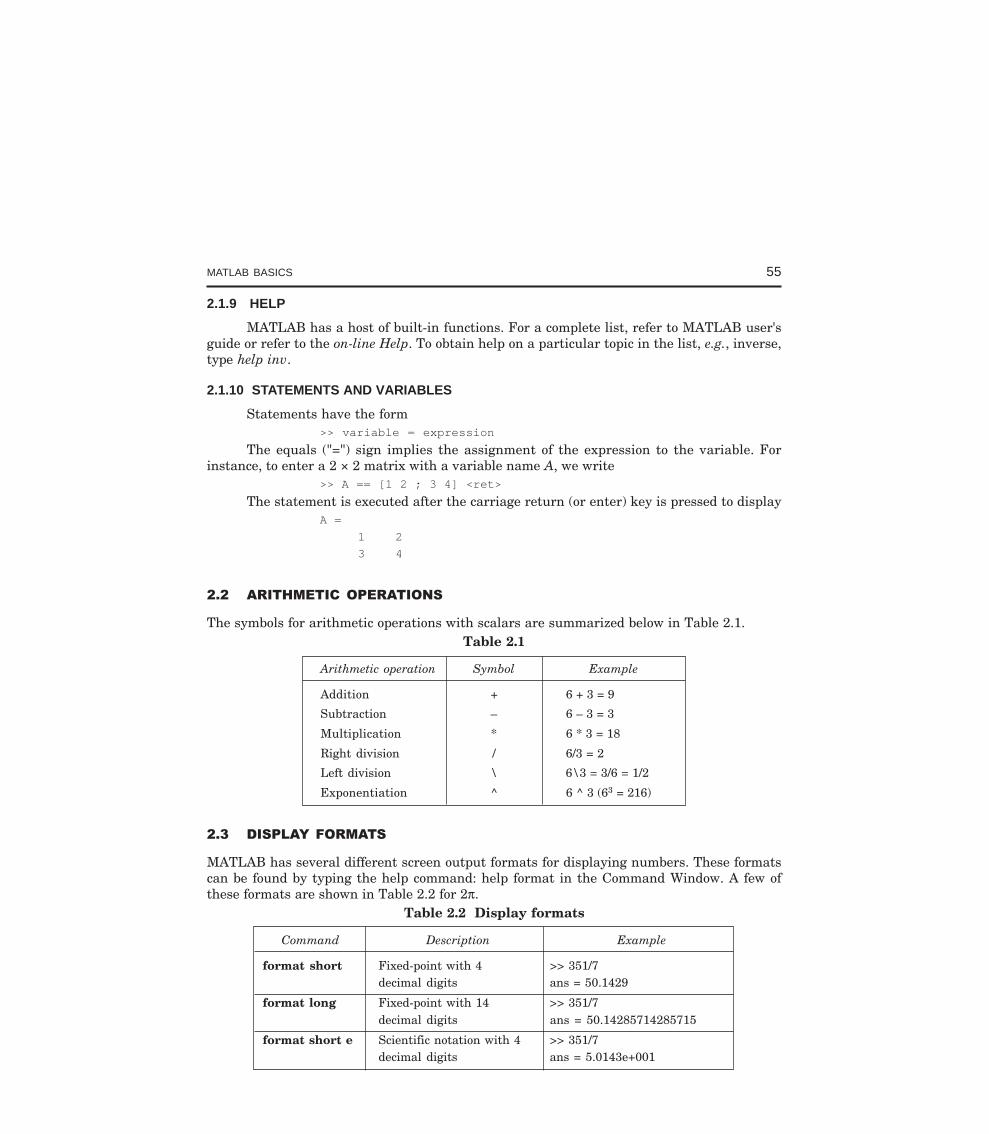
MATLAB BASICS 55
2.1.9 HELP
MATLAB has a host of built-in functions. For a complete list, refer to MATLAB user'sguide or refer to the on-line Help. To obtain help on a particular topic in the list, e.g., inverse,type help inv.
2.1.10 STATEMENTS AND VARIABLES
Statements have the form>> variable = expression
The equals ("=") sign implies the assignment of the expression to the variable. Forinstance, to enter a 2 × 2 matrix with a variable name A, we write
>> A == [1 2 ; 3 4] <ret>
The statement is executed after the carriage return (or enter) key is pressed to displayA =
1 2
3 4
The symbols for arithmetic operations with scalars are summarized below in Table 2.1.Table 2.1
Arithmetic operation Symbol Example
Addition + 6 + 3 = 9
Subtraction – 6 – 3 = 3
Multiplication * 6 * 3 = 18
Right division / 6/3 = 2
Left division \ 6\3 = 3/6 = 1/2
Exponentiation ^ 6 ^ 3 (63 = 216)
MATLAB has several different screen output formats for displaying numbers. These formatscan be found by typing the help command: help format in the Command Window. A few ofthese formats are shown in Table 2.2 for 2π.
Table 2.2 Display formats
Command Description Example
format short Fixed-point with 4 >> 351/7decimal digits ans = 50.1429
format long Fixed-point with 14 >> 351/7decimal digits ans = 50.14285714285715
format short e Scientific notation with 4 >> 351/7decimal digits ans = 5.0143e+001
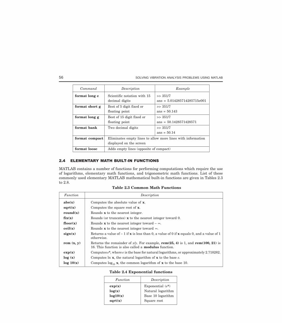
56 SOLVING VIBRATION ANALYSIS PROBLEMS USING MATLAB
Command Description Example
format long e Scientific notation with 15 >> 351/7decimal digits ans = 5.014285714285715e001
format short g Best of 5 digit fixed or >> 351/7floating point ans = 50.143
format long g Best of 15 digit fixed or >> 351/7floating point ans = 50.1428571428571
format bank Two decimal digits >> 351/7ans = 50.14
format compact Eliminates empty lines to allow more lines with informationdisplayed on the screen
format loose Adds empty lines (opposite of compact)
MATLAB contains a number of functions for performing computations which require the useof logarithms, elementary math functions, and trigonometric math functions. List of thesecommonly used elementary MATLAB mathematical built-in functions are given in Tables 2.3to 2.8.
Table 2.3 Common Math Functions
Function Description
abs(x) Computes the absolute value of x.
sqrt(x) Computes the square root of x.
round(x) Rounds x to the nearest integer.
fix(x) Rounds (or truncates) x to the nearest integer toward 0.
floor(x) Rounds x to the nearest integer toward – ∞.
ceil(x) Rounds x to the nearest integer toward ∞.
sign(x) Returns a value of – 1 if x is less than 0, a value of 0 if x equals 0, and a value of 1otherwise.
rem (x, y) Returns the remainder of x/y. For example, rem(25, 4) is 1, and rem(100, 21) is16. This function is also called a modulus function.
exp(x) Computes ex, where e is the base for natural logarithms, or approximately 2.718282.
log (x) Computes ln x, the natural logarithm of x to the base e.
log 10(x) Computes log10 x, the common logarithm of x to the base 10.
Table 2.4 Exponential functions
Function Description
exp(x) Exponential (ex)log(x) Natural logarithmlog10(x) Base 10 logarithmsqrt(x) Square root
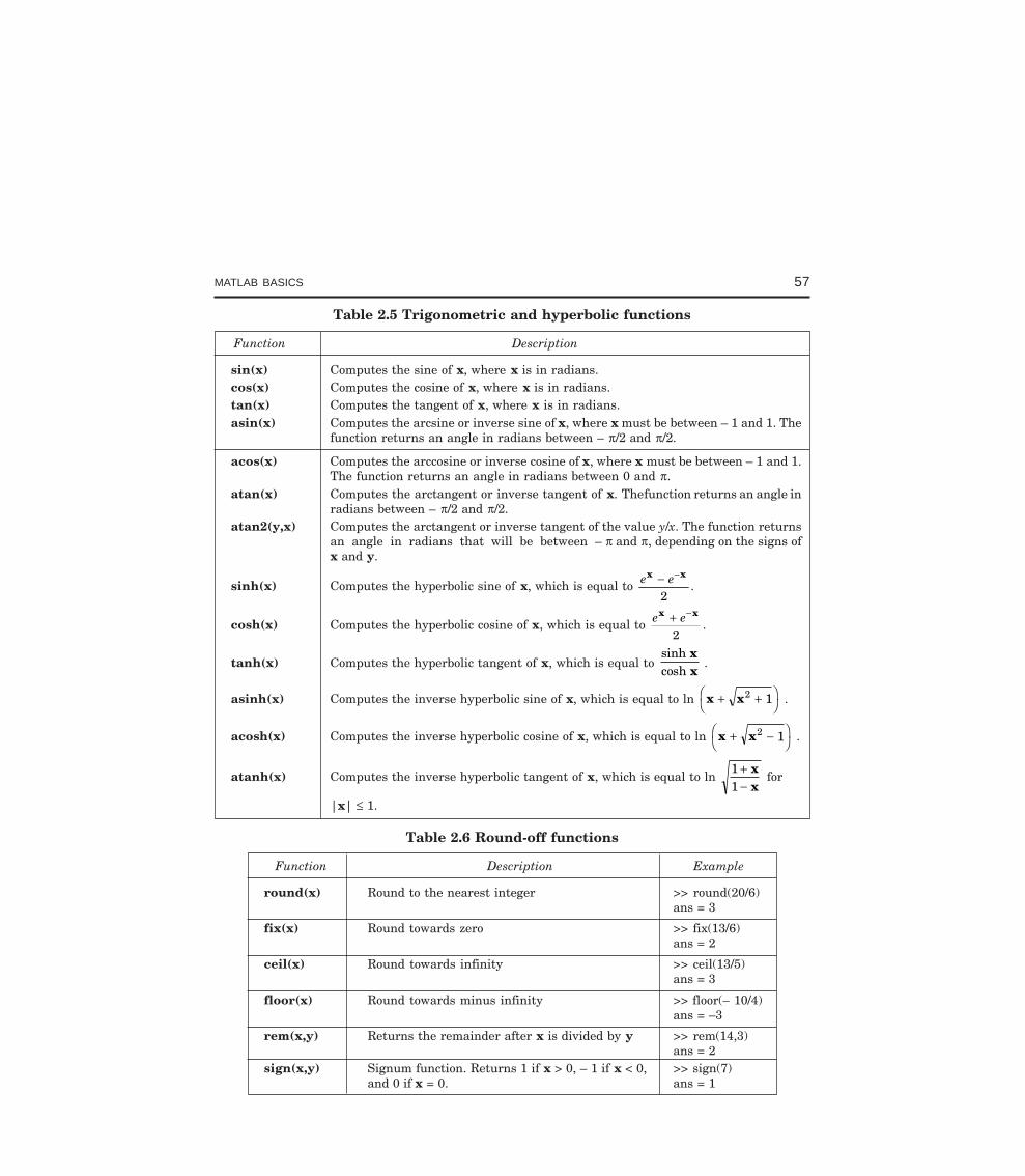
MATLAB BASICS 57
Table 2.5 Trigonometric and hyperbolic functions
Function Description
sin(x) Computes the sine of x, where x is in radians.cos(x) Computes the cosine of x, where x is in radians.tan(x) Computes the tangent of x, where x is in radians.asin(x) Computes the arcsine or inverse sine of x, where x must be between – 1 and 1. The
function returns an angle in radians between – π/2 and π/2.
acos(x) Computes the arccosine or inverse cosine of x, where x must be between – 1 and 1.The function returns an angle in radians between 0 and π.
atan(x) Computes the arctangent or inverse tangent of x. Thefunction returns an angle inradians between – π/2 and π/2.
atan2(y,x) Computes the arctangent or inverse tangent of the value y/x. The function returnsan angle in radians that will be between – π and π, depending on the signs ofx and y.
sinh(x) Computes the hyperbolic sine of x, which is equal to e ex x− −
2.
cosh(x) Computes the hyperbolic cosine of x, which is equal to e ex x+ −
2.
tanh(x) Computes the hyperbolic tangent of x, which is equal to sinhcosh
xx
.
asinh(x) Computes the inverse hyperbolic sine of x, which is equal to ln x x+ +FH
IK
2 1 .
acosh(x) Computes the inverse hyperbolic cosine of x, which is equal to ln x x+ −FH
IK
2 1 .
atanh(x) Computes the inverse hyperbolic tangent of x, which is equal to ln 11
+−
xx
for
|x| ≤ 1.
Table 2.6 Round-off functions
Function Description Example
round(x) Round to the nearest integer >> round(20/6)ans = 3
fix(x) Round towards zero >> fix(13/6)ans = 2
ceil(x) Round towards infinity >> ceil(13/5)ans = 3
floor(x) Round towards minus infinity >> floor(– 10/4)ans = –3
rem(x,y) Returns the remainder after x is divided by y >> rem(14,3)ans = 2
sign(x,y) Signum function. Returns 1 if x > 0, – 1 if x < 0, >> sign(7)and 0 if x = 0. ans = 1
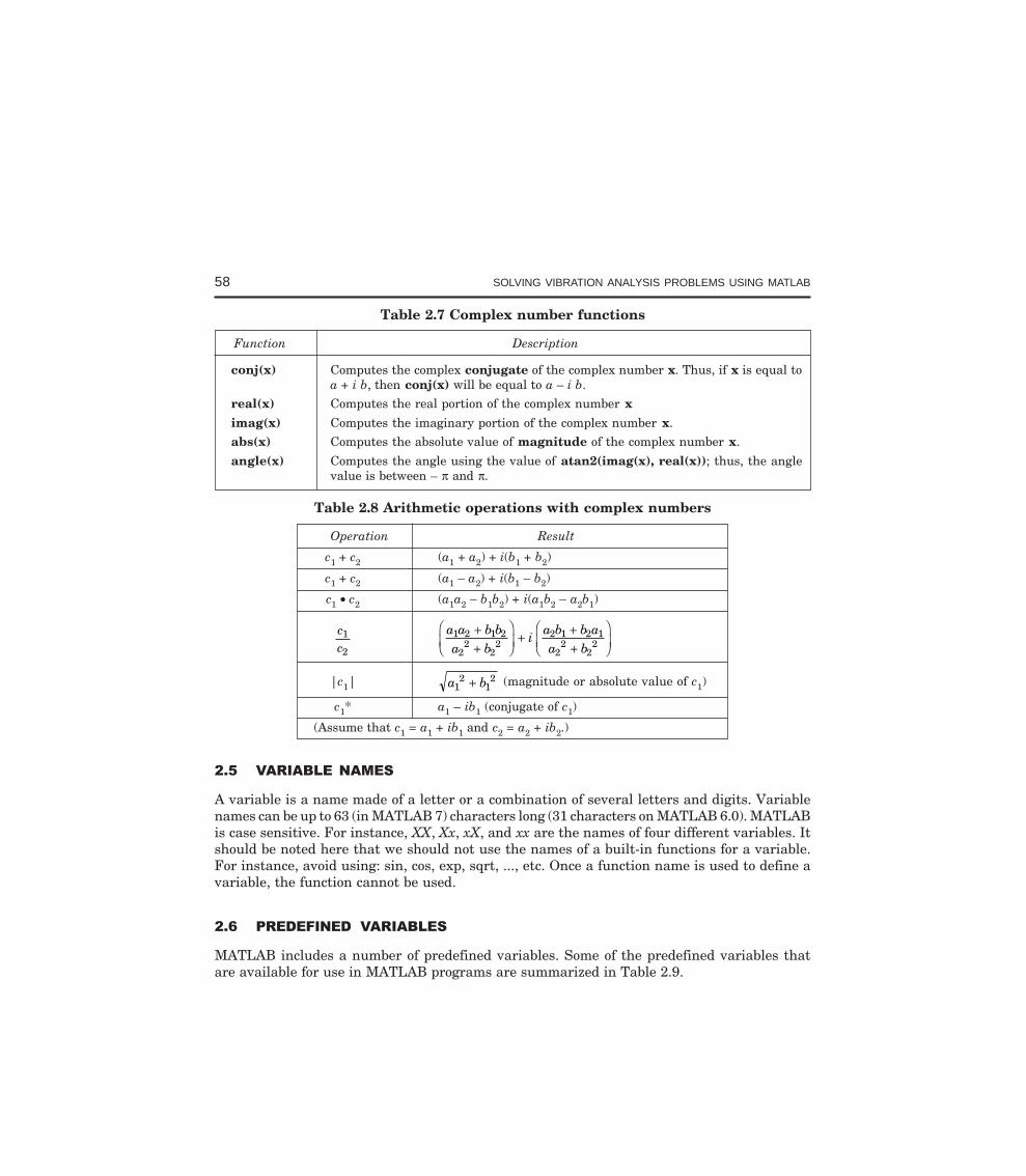
58 SOLVING VIBRATION ANALYSIS PROBLEMS USING MATLAB
Table 2.7 Complex number functions
Function Description
conj(x) Computes the complex conjugate of the complex number x. Thus, if x is equal toa + i b, then conj(x) will be equal to a – i b.
real(x) Computes the real portion of the complex number ximag(x) Computes the imaginary portion of the complex number x.
abs(x) Computes the absolute value of magnitude of the complex number x.
angle(x) Computes the angle using the value of atan2(imag(x), real(x)); thus, the anglevalue is between – π and π.
Table 2.8 Arithmetic operations with complex numbers
Operation Result
c1 + c2 (a1 + a2) + i(b1 + b2)
c1 + c2 (a1 – a2) + i(b1 – b2)
c1 • c2 (a1a2 – b1b2) + i(a1b2 – a2b1)
cc1
2
a a b ba b
ia b b aa b
1 2 1 2
22
22
2 1 2 1
22
22
++
FHG
IKJ
+ ++
FHG
IKJ
|c1| a b12
12+ (magnitude or absolute value of c1)
c1* a1 – ib1 (conjugate of c1)
(Assume that c1 = a1 + ib1 and c2 = a2 + ib2.)
A variable is a name made of a letter or a combination of several letters and digits. Variablenames can be up to 63 (in MATLAB 7) characters long (31 characters on MATLAB 6.0). MATLABis case sensitive. For instance, XX, Xx, xX, and xx are the names of four different variables. Itshould be noted here that we should not use the names of a built-in functions for a variable.For instance, avoid using: sin, cos, exp, sqrt, ..., etc. Once a function name is used to define avariable, the function cannot be used.
MATLAB includes a number of predefined variables. Some of the predefined variables thatare available for use in MATLAB programs are summarized in Table 2.9.
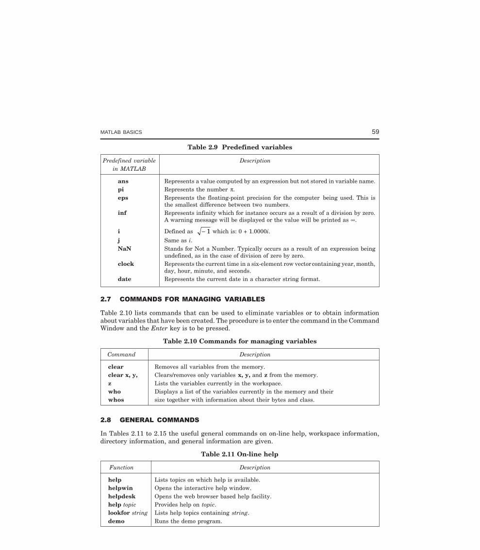
MATLAB BASICS 59
Table 2.9 Predefined variables
Predefined variable Descriptionin MATLAB
ans Represents a value computed by an expression but not stored in variable name.pi Represents the number π.eps Represents the floating-point precision for the computer being used. This is
the smallest difference between two numbers.inf Represents infinity which for instance occurs as a result of a division by zero.
A warning message will be displayed or the value will be printed as ∞.
i Defined as − 1 which is: 0 + 1.0000i.
j Same as i.NaN Stands for Not a Number. Typically occurs as a result of an expression being
undefined, as in the case of division of zero by zero.clock Represents the current time in a six-element row vector containing year, month,
day, hour, minute, and seconds.date Represents the current date in a character string format.
Table 2.10 lists commands that can be used to eliminate variables or to obtain informationabout variables that have been created. The procedure is to enter the command in the CommandWindow and the Enter key is to be pressed.
Table 2.10 Commands for managing variables
Command Description
clear Removes all variables from the memory.clear x, y, Clears/removes only variables x, y, and z from the memory.z Lists the variables currently in the workspace.who Displays a list of the variables currently in the memory and theirwhos size together with information about their bytes and class.
In Tables 2.11 to 2.15 the useful general commands on on-line help, workspace information,directory information, and general information are given.
Table 2.11 On-line help
Function Description
help Lists topics on which help is available.helpwin Opens the interactive help window.helpdesk Opens the web browser based help facility.help topic Provides help on topic.lookfor string Lists help topics containing string.demo Runs the demo program.
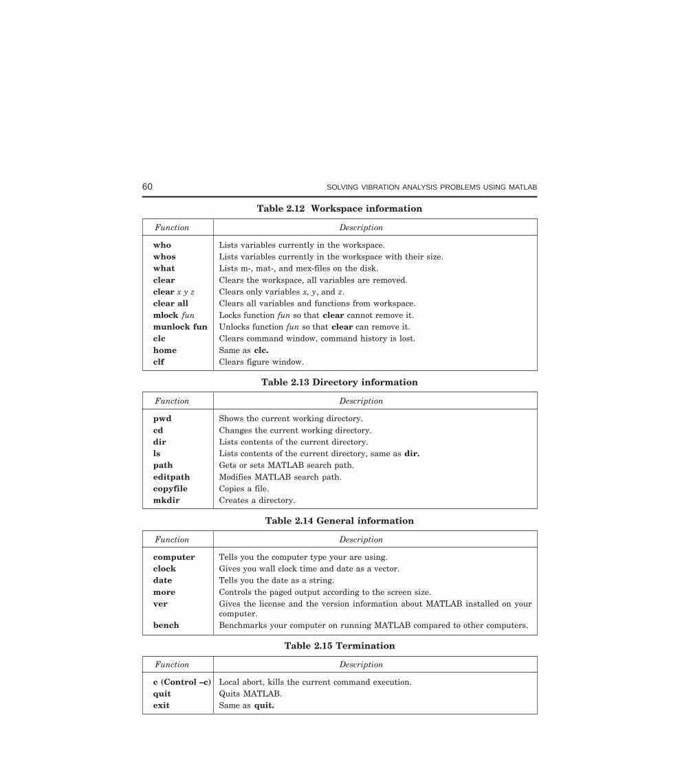
60 SOLVING VIBRATION ANALYSIS PROBLEMS USING MATLAB
Table 2.12 Workspace information
Function Description
who Lists variables currently in the workspace.whos Lists variables currently in the workspace with their size.what Lists m-, mat-, and mex-files on the disk.clear Clears the workspace, all variables are removed.clear x y z Clears only variables x, y, and z.clear all Clears all variables and functions from workspace.mlock fun Locks function fun so that clear cannot remove it.munlock fun Unlocks function fun so that clear can remove it.clc Clears command window, command history is lost.home Same as clc.clf Clears figure window.
Table 2.13 Directory information
Function Description
pwd Shows the current working directory.cd Changes the current working directory.dir Lists contents of the current directory.ls Lists contents of the current directory, same as dir.path Gets or sets MATLAB search path.editpath Modifies MATLAB search path.copyfile Copies a file.mkdir Creates a directory.
Table 2.14 General information
Function Description
computer Tells you the computer type your are using.clock Gives you wall clock time and date as a vector.date Tells you the date as a string.more Controls the paged output according to the screen size.ver Gives the license and the version information about MATLAB installed on your
computer.bench Benchmarks your computer on running MATLAB compared to other computers.
Table 2.15 Termination
Function Description
c (Control –c) Local abort, kills the current command execution.quit Quits MATLAB.exit Same as quit.
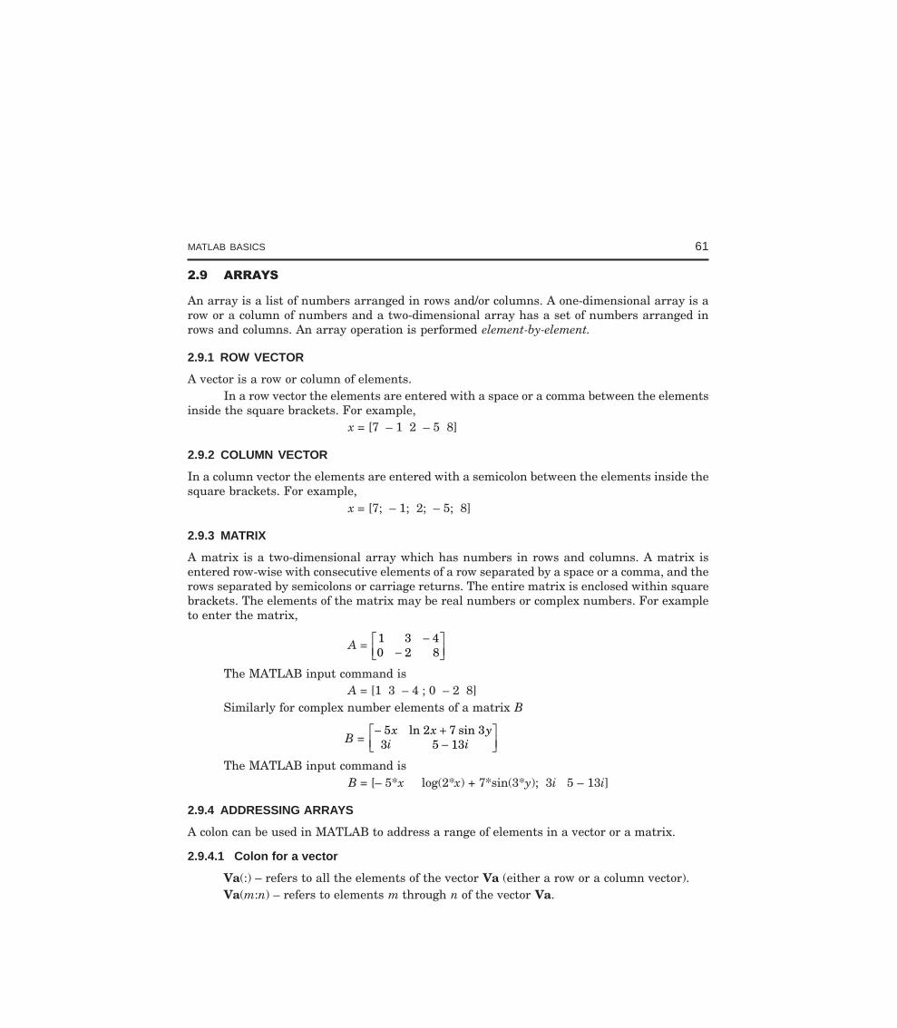
MATLAB BASICS 61
An array is a list of numbers arranged in rows and/or columns. A one-dimensional array is arow or a column of numbers and a two-dimensional array has a set of numbers arranged inrows and columns. An array operation is performed element-by-element.
2.9.1 ROW VECTOR
A vector is a row or column of elements.In a row vector the elements are entered with a space or a comma between the elements
inside the square brackets. For example,x = [7 – 1 2 – 5 8]
2.9.2 COLUMN VECTOR
In a column vector the elements are entered with a semicolon between the elements inside thesquare brackets. For example,
x = [7; – 1; 2; – 5; 8]
2.9.3 MATRIX
A matrix is a two-dimensional array which has numbers in rows and columns. A matrix isentered row-wise with consecutive elements of a row separated by a space or a comma, and therows separated by semicolons or carriage returns. The entire matrix is enclosed within squarebrackets. The elements of the matrix may be real numbers or complex numbers. For exampleto enter the matrix,
A = 1 3 40 2 8
−−
LNM
OQP
The MATLAB input command isA = [1 3 – 4 ; 0 – 2 8]
Similarly for complex number elements of a matrix B
B = − +
−LNM
OQP
5 2 7 33 5 13
x x yi i
ln sin
The MATLAB input command isB = [– 5*x log(2*x) + 7*sin(3*y); 3i 5 – 13i]
2.9.4 ADDRESSING ARRAYS
A colon can be used in MATLAB to address a range of elements in a vector or a matrix.
2.9.4.1 Colon for a vector
Va(:) – refers to all the elements of the vector Va (either a row or a column vector).Va(m:n) – refers to elements m through n of the vector Va.
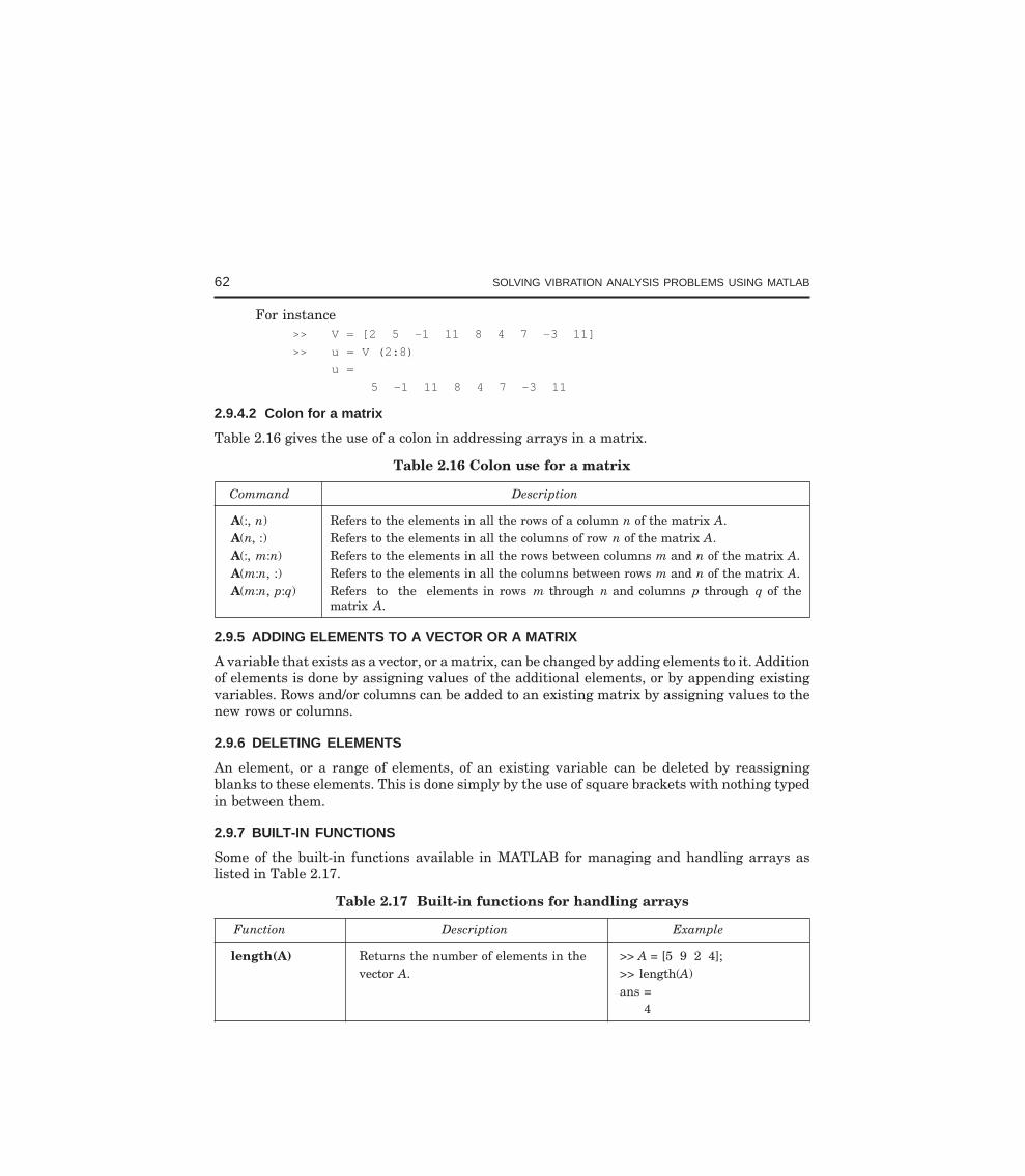
62 SOLVING VIBRATION ANALYSIS PROBLEMS USING MATLAB
For instance>> V = [2 5 –1 11 8 4 7 –3 11]
>> u = V (2:8)
u =
5 –1 11 8 4 7 –3 11
2.9.4.2 Colon for a matrix
Table 2.16 gives the use of a colon in addressing arrays in a matrix.
Table 2.16 Colon use for a matrix
Command Description
A(:, n) Refers to the elements in all the rows of a column n of the matrix A.A(n, :) Refers to the elements in all the columns of row n of the matrix A.A(:, m:n) Refers to the elements in all the rows between columns m and n of the matrix A.A(m:n, :) Refers to the elements in all the columns between rows m and n of the matrix A.A(m:n, p:q) Refers to the elements in rows m through n and columns p through q of the
matrix A.
2.9.5 ADDING ELEMENTS TO A VECTOR OR A MATRIX
A variable that exists as a vector, or a matrix, can be changed by adding elements to it. Additionof elements is done by assigning values of the additional elements, or by appending existingvariables. Rows and/or columns can be added to an existing matrix by assigning values to thenew rows or columns.
2.9.6 DELETING ELEMENTS
An element, or a range of elements, of an existing variable can be deleted by reassigningblanks to these elements. This is done simply by the use of square brackets with nothing typedin between them.
2.9.7 BUILT-IN FUNCTIONS
Some of the built-in functions available in MATLAB for managing and handling arrays aslisted in Table 2.17.
Table 2.17 Built-in functions for handling arrays
Function Description Example
length(A) Returns the number of elements in the >> A = [5 9 2 4];vector A. >> length(A)
ans =4
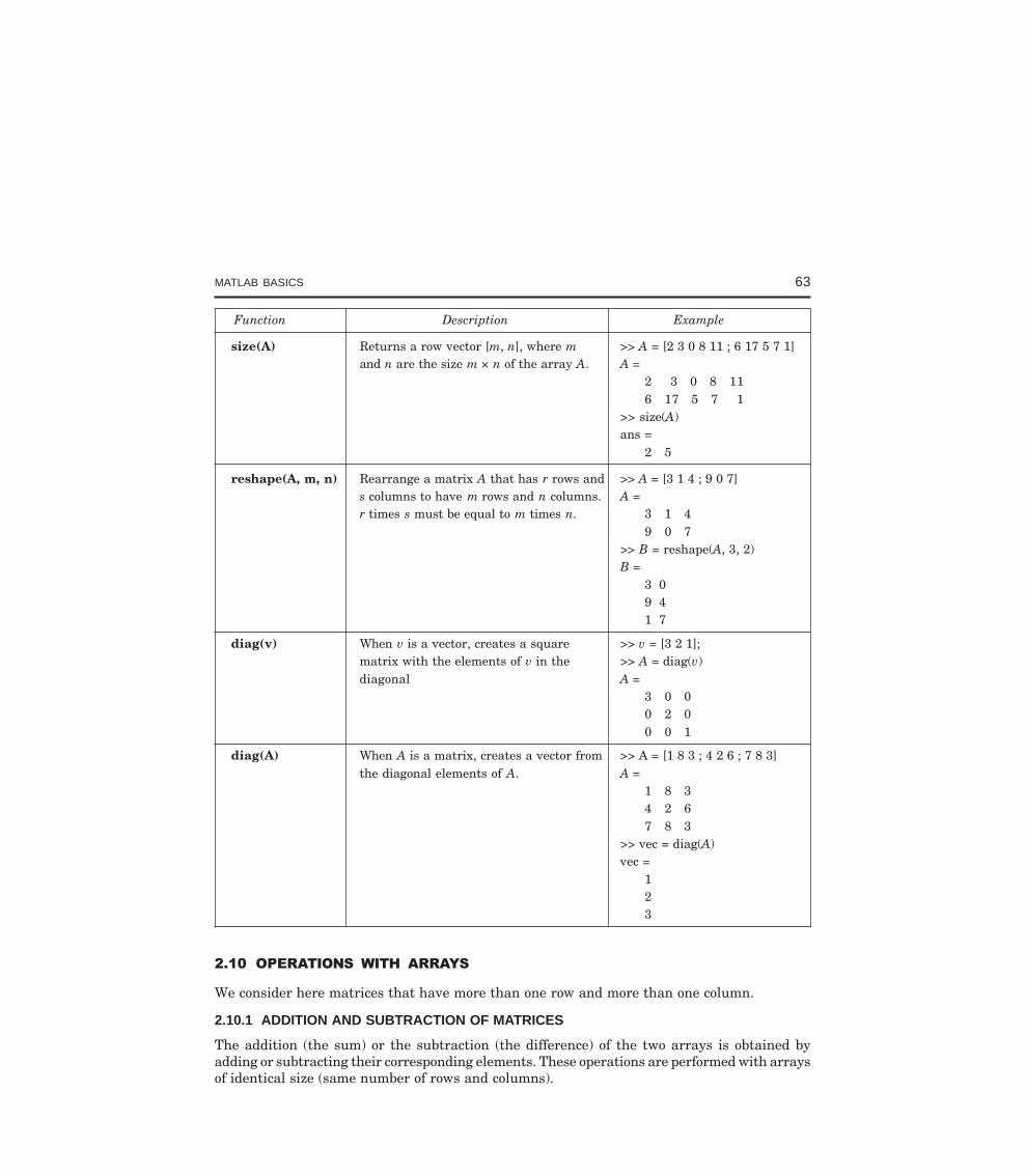
MATLAB BASICS 63
Function Description Example
size(A) Returns a row vector [m, n], where m >> A = [2 3 0 8 11 ; 6 17 5 7 1]and n are the size m × n of the array A. A =
2 3 0 8 116 17 5 7 1
>> size(A)ans =
2 5
reshape(A, m, n) Rearrange a matrix A that has r rows and >> A = [3 1 4 ; 9 0 7]s columns to have m rows and n columns. A =r times s must be equal to m times n. 3 1 4
9 0 7>> B = reshape(A, 3, 2)B =
3 09 41 7
diag(v) When v is a vector, creates a square >> v = [3 2 1];matrix with the elements of v in the >> A = diag(v)diagonal A =
3 0 00 2 00 0 1
diag(A) When A is a matrix, creates a vector from >> A = [1 8 3 ; 4 2 6 ; 7 8 3]the diagonal elements of A. A =
1 8 34 2 67 8 3
>> vec = diag(A)vec =
123
! "
We consider here matrices that have more than one row and more than one column.
2.10.1 ADDITION AND SUBTRACTION OF MATRICES
The addition (the sum) or the subtraction (the difference) of the two arrays is obtained byadding or subtracting their corresponding elements. These operations are performed with arraysof identical size (same number of rows and columns).
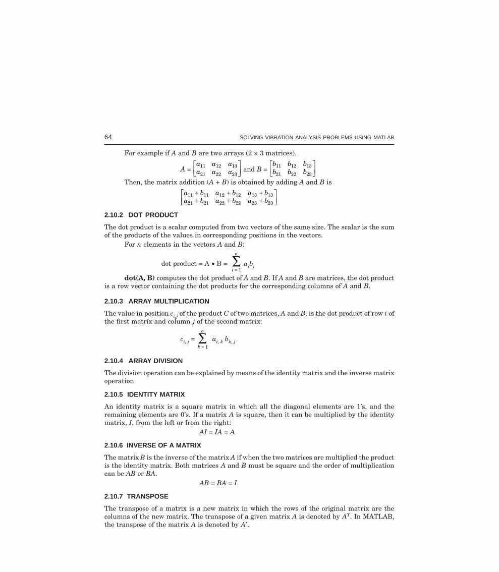
64 SOLVING VIBRATION ANALYSIS PROBLEMS USING MATLAB
For example if A and B are two arrays (2 × 3 matrices).
A = a a aa a a
11 12 13
21 22 23
LNM
OQP and B =
b b bb b b
11 12 13
21 22 23
LNM
OQP
Then, the matrix addition (A + B) is obtained by adding A and B is
a b a b a ba b a b a b
11 11 12 12 13 13
21 21 22 22 23 23
+ + ++ + +
LNM
OQP
2.10.2 DOT PRODUCT
The dot product is a scalar computed from two vectors of the same size. The scalar is the sumof the products of the values in corresponding positions in the vectors.
For n elements in the vectors A and B:
dot product = A • B = i
n
=∑
1aibi
dot(A, B) computes the dot product of A and B. If A and B are matrices, the dot productis a row vector containing the dot products for the corresponding columns of A and B.
2.10.3 ARRAY MULTIPLICATION
The value in position ci,j of the product C of two matrices, A and B, is the dot product of row i ofthe first matrix and column j of the second matrix:
ci, j = k
n
=∑
1
ai, k bk, j
2.10.4 ARRAY DIVISION
The division operation can be explained by means of the identity matrix and the inverse matrixoperation.
2.10.5 IDENTITY MATRIX
An identity matrix is a square matrix in which all the diagonal elements are 1’s, and theremaining elements are 0’s. If a matrix A is square, then it can be multiplied by the identitymatrix, I, from the left or from the right:
AI = IA = A
2.10.6 INVERSE OF A MATRIX
The matrix B is the inverse of the matrix A if when the two matrices are multiplied the productis the identity matrix. Both matrices A and B must be square and the order of multiplicationcan be AB or BA.
AB = BA = I
2.10.7 TRANSPOSE
The transpose of a matrix is a new matrix in which the rows of the original matrix are thecolumns of the new matrix. The transpose of a given matrix A is denoted by AT. In MATLAB,the transpose of the matrix A is denoted by A′.
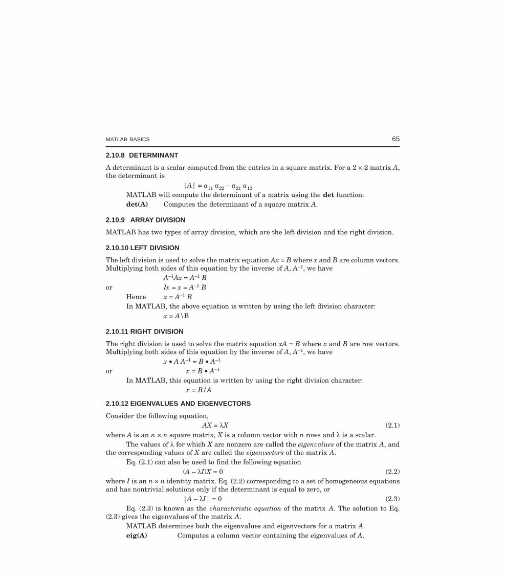
MATLAB BASICS 65
2.10.8 DETERMINANT
A determinant is a scalar computed from the entries in a square matrix. For a 2 × 2 matrix A,the determinant is
|A| = a11 a22 – a21 a12MATLAB will compute the determinant of a matrix using the det function:det(A) Computes the determinant of a square matrix A.
2.10.9 ARRAY DIVISION
MATLAB has two types of array division, which are the left division and the right division.
2.10.10 LEFT DIVISION
The left division is used to solve the matrix equation Ax = B where x and B are column vectors.Multiplying both sides of this equation by the inverse of A, A–1, we have
A–1Ax = A–1 Bor Ix = x = A–1 B
Hence x = A–1 BIn MATLAB, the above equation is written by using the left division character:
x = A\B
2.10.11 RIGHT DIVISION
The right division is used to solve the matrix equation xA = B where x and B are row vectors.Multiplying both sides of this equation by the inverse of A, A–1, we have
x • A A–1 = B • A–1
or x = B • A–1
In MATLAB, this equation is written by using the right division character:x = B/A
2.10.12 EIGENVALUES AND EIGENVECTORS
Consider the following equation,AX = λX (2.1)
where A is an n × n square matrix, X is a column vector with n rows and λ is a scalar.The values of λ for which X are nonzero are called the eigenvalues of the matrix A, and
the corresponding values of X are called the eigenvectors of the matrix A.Eq. (2.1) can also be used to find the following equation
(A – λI)X = 0 (2.2)where I is an n × n identity matrix. Eq. (2.2) corresponding to a set of homogeneous equationsand has nontrivial solutions only if the determinant is equal to zero, or
|A – λI| = 0 (2.3)Eq. (2.3) is known as the characteristic equation of the matrix A. The solution to Eq.
(2.3) gives the eigenvalues of the matrix A.MATLAB determines both the eigenvalues and eigenvectors for a matrix A.eig(A) Computes a column vector containing the eigenvalues of A.
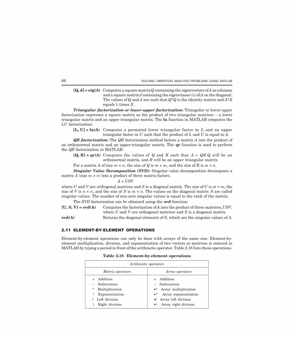
66 SOLVING VIBRATION ANALYSIS PROBLEMS USING MATLAB
[Q, d] = eig(A) Computes a square matrix Q containing the eigenvectors of A as columnsand a square matrix d containing the eigenvlaues (λ) of A on the diagonal.The values of Q and d are such that Q*Q is the identity matrix and A*Xequals λ times X.
Triangular factorization or lower-upper factorization: Triangular or lower-upperfactorization expresses a square matrix as the product of two triangular matrices – a lowertriangular matrix and an upper triangular matrix. The lu function in MATLAB computes theLU factorization:
[L, U] = lu(A) Computes a permuted lower triangular factor in L and an uppertriangular factor in U such that the product of L and U is equal to A.
QR factorization: The QR factorization method factors a matrix A into the product ofan orthonormal matrix and an upper-triangular matrix. The qr function is used to performthe QR factorization in MATLAB:
[Q, R] = qr(A) Computes the values of Q and R such that A = QR.Q will be anorthonormal matrix, and R will be an upper triangular matrix.
For a matrix A of size m × n, the size of Q is m × m, and the size of R is m × n.Singular Value Decomposition (SVD): Singular value decomposition decomposes a
matrix A (size m × n) into a product of three matrix factors.A = USV
where U and V are orthogonal matrices and S is a diagonal matrix. The size of U is m × m, thesize of V is n × n, and the size of S is m × n. The values on the diagonal matrix S are calledsingular values. The number of non-zero singular values is equal to the rank of the matrix.
The SVD factorization can be obtained using the svd function:[U, S, V] = svd(A) Computes the factorization of A into the product of three matrices, USV,
where U and V are orthogonal matrices and S is a diagonal matrix.svd(A) Returns the diagonal elements of S, which are the singular values of A.
Element-by-element operations can only be done with arrays of the same size. Element-by-element multiplication, division, and exponentiation of two vectors or matrices is entered inMATLAB by typing a period in front of the arithmetic operator. Table 2.18 lists these operations.
Table 2.18 Element-by-element operations
Arithmetic operators
Matrix operators Array operators
+ Addition + Addition– Subtraction – Subtraction* Multiplication •* Array multiplication^ Exponentiation •^ Array exponentiation/ Left division •/ Array left division\ Right division •\ Array right division
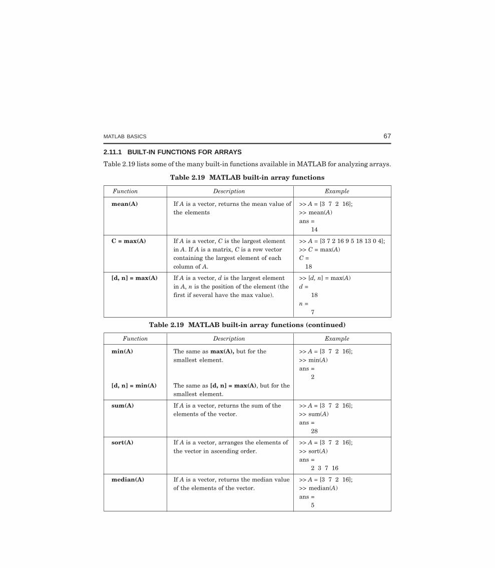
MATLAB BASICS 67
2.11.1 BUILT-IN FUNCTIONS FOR ARRAYS
Table 2.19 lists some of the many built-in functions available in MATLAB for analyzing arrays.
Table 2.19 MATLAB built-in array functions
Function Description Example
mean(A) If A is a vector, returns the mean value of >> A = [3 7 2 16];the elements >> mean(A)
ans =14
C = max(A) If A is a vector, C is the largest element >> A = [3 7 2 16 9 5 18 13 0 4];in A. If A is a matrix, C is a row vector >> C = max(A)containing the largest element of each C =column of A. 18
[d, n] = max(A) If A is a vector, d is the largest element >> [d, n] = max(A)in A, n is the position of the element (the d =first if several have the max value). 18
n =7
Table 2.19 MATLAB built-in array functions (continued)
Function Description Example
min(A) The same as max(A), but for the >> A = [3 7 2 16];smallest element. >> min(A)
ans =2
[d, n] = min(A) The same as [d, n] = max(A), but for thesmallest element.
sum(A) If A is a vector, returns the sum of the >> A = [3 7 2 16];elements of the vector. >> sum(A)
ans =28
sort(A) If A is a vector, arranges the elements of >> A = [3 7 2 16];the vector in ascending order. >> sort(A)
ans =2 3 7 16
median(A) If A is a vector, returns the median value >> A = [3 7 2 16];of the elements of the vector. >> median(A)
ans =5
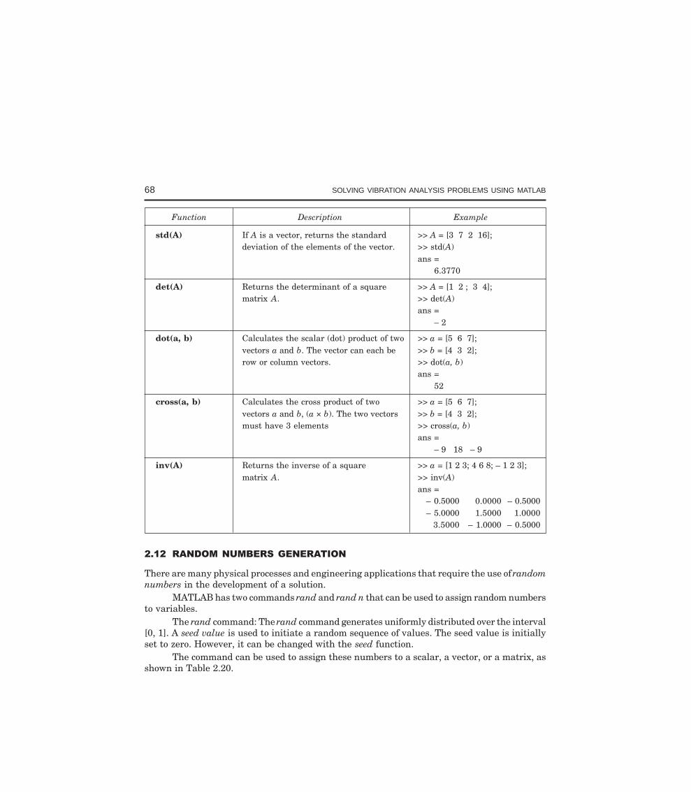
68 SOLVING VIBRATION ANALYSIS PROBLEMS USING MATLAB
Function Description Example
std(A) If A is a vector, returns the standard >> A = [3 7 2 16];deviation of the elements of the vector. >> std(A)
ans =6.3770
det(A) Returns the determinant of a square >> A = [1 2 ; 3 4];matrix A. >> det(A)
ans =– 2
dot(a, b) Calculates the scalar (dot) product of two >> a = [5 6 7];vectors a and b. The vector can each be >> b = [4 3 2];row or column vectors. >> dot(a, b)
ans =52
cross(a, b) Calculates the cross product of two >> a = [5 6 7];vectors a and b, (a × b). The two vectors >> b = [4 3 2];must have 3 elements >> cross(a, b)
ans =– 9 18 – 9
inv(A) Returns the inverse of a square >> a = [1 2 3; 4 6 8; – 1 2 3];matrix A. >> inv(A)
ans =– 0.5000 0.0000 – 0.5000– 5.0000 1.5000 1.0000
3.5000 – 1.0000 – 0.5000
There are many physical processes and engineering applications that require the use of randomnumbers in the development of a solution.
MATLAB has two commands rand and rand n that can be used to assign random numbersto variables.
The rand command: The rand command generates uniformly distributed over the interval[0, 1]. A seed value is used to initiate a random sequence of values. The seed value is initiallyset to zero. However, it can be changed with the seed function.
The command can be used to assign these numbers to a scalar, a vector, or a matrix, asshown in Table 2.20.
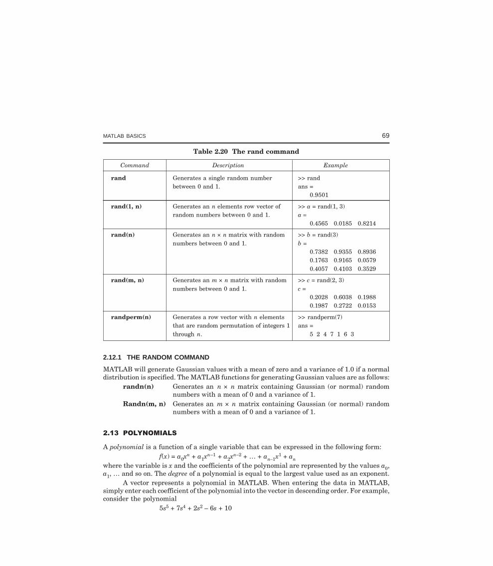
MATLAB BASICS 69
Table 2.20 The rand command
Command Description Example
rand Generates a single random number >> randbetween 0 and 1. ans =
0.9501
rand(1, n) Generates an n elements row vector of >> a = rand(1, 3)random numbers between 0 and 1. a =
0.4565 0.0185 0.8214
rand(n) Generates an n × n matrix with random >> b = rand(3)numbers between 0 and 1. b =
0.7382 0.9355 0.89360.1763 0.9165 0.05790.4057 0.4103 0.3529
rand(m, n) Generates an m × n matrix with random >> c = rand(2, 3)numbers between 0 and 1. c =
0.2028 0.6038 0.19880.1987 0.2722 0.0153
randperm(n) Generates a row vector with n elements >> randperm(7)that are random permutation of integers 1 ans =through n. 5 2 4 7 1 6 3
2.12.1 THE RANDOM COMMAND
MATLAB will generate Gaussian values with a mean of zero and a variance of 1.0 if a normaldistribution is specified. The MATLAB functions for generating Gaussian values are as follows:
randn(n) Generates an n × n matrix containing Gaussian (or normal) randomnumbers with a mean of 0 and a variance of 1.
Randn(m, n) Generates an m × n matrix containing Gaussian (or normal) randomnumbers with a mean of 0 and a variance of 1.
A polynomial is a function of a single variable that can be expressed in the following form:f(x) = a0x
n + a1xn–1 + a2x
n–2 + … + an–1x1 + anwhere the variable is x and the coefficients of the polynomial are represented by the values a0,a1, … and so on. The degree of a polynomial is equal to the largest value used as an exponent.
A vector represents a polynomial in MATLAB. When entering the data in MATLAB,simply enter each coefficient of the polynomial into the vector in descending order. For example,consider the polynomial
5s5 + 7s4 + 2s2 – 6s + 10
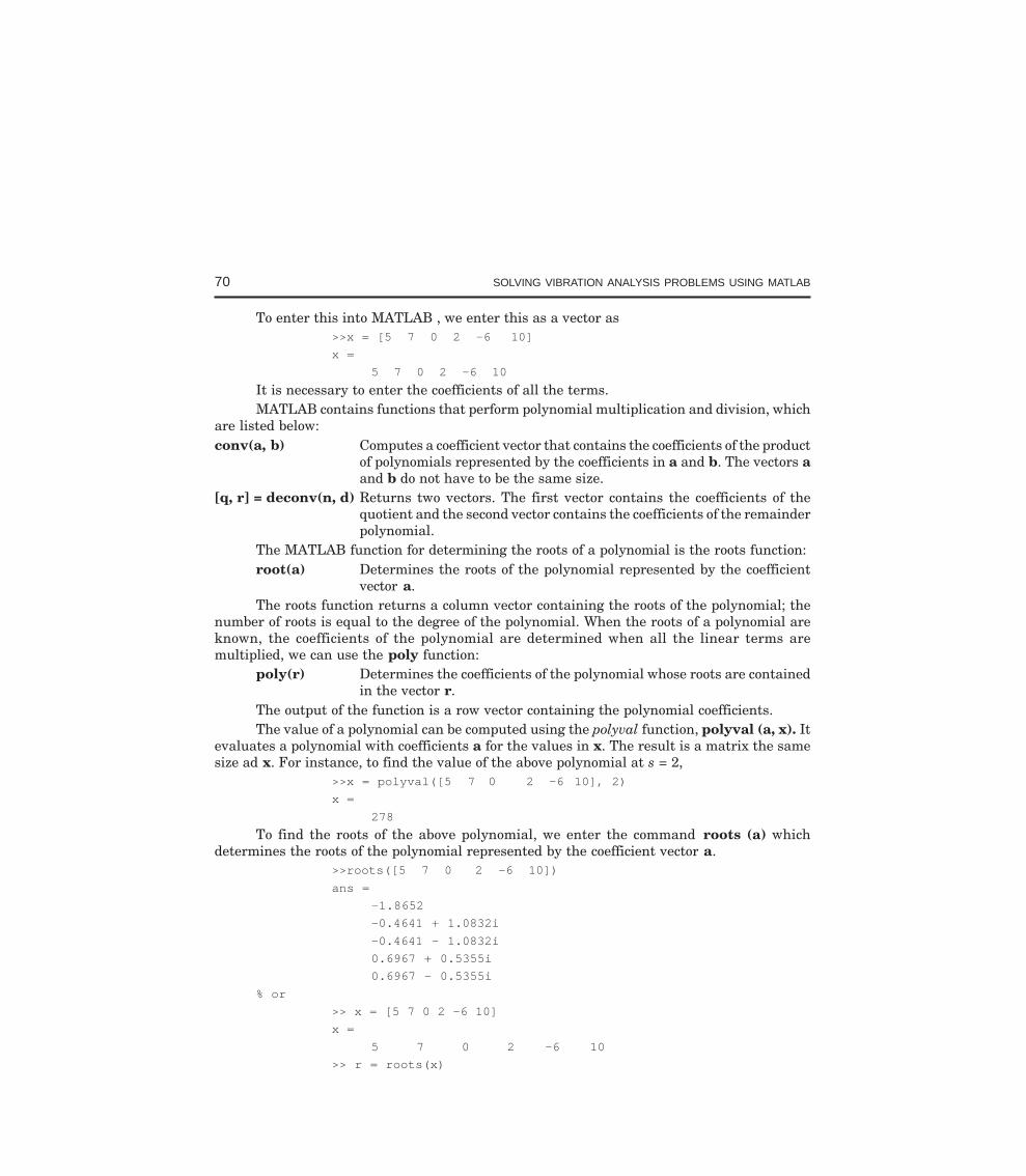
70 SOLVING VIBRATION ANALYSIS PROBLEMS USING MATLAB
To enter this into MATLAB , we enter this as a vector as>>x = [5 7 0 2 –6 10]
x =
5 7 0 2 –6 10
It is necessary to enter the coefficients of all the terms.MATLAB contains functions that perform polynomial multiplication and division, which
are listed below:conv(a, b) Computes a coefficient vector that contains the coefficients of the product
of polynomials represented by the coefficients in a and b. The vectors aand b do not have to be the same size.
[q, r] = deconv(n, d) Returns two vectors. The first vector contains the coefficients of thequotient and the second vector contains the coefficients of the remainderpolynomial.
The MATLAB function for determining the roots of a polynomial is the roots function:root(a) Determines the roots of the polynomial represented by the coefficient
vector a.The roots function returns a column vector containing the roots of the polynomial; the
number of roots is equal to the degree of the polynomial. When the roots of a polynomial areknown, the coefficients of the polynomial are determined when all the linear terms aremultiplied, we can use the poly function:
poly(r) Determines the coefficients of the polynomial whose roots are containedin the vector r.
The output of the function is a row vector containing the polynomial coefficients.The value of a polynomial can be computed using the polyval function, polyval (a, x). It
evaluates a polynomial with coefficients a for the values in x. The result is a matrix the samesize ad x. For instance, to find the value of the above polynomial at s = 2,
>>x = polyval([5 7 0 2 -6 10], 2)
x =
278
To find the roots of the above polynomial, we enter the command roots (a) whichdetermines the roots of the polynomial represented by the coefficient vector a.
>>roots([5 7 0 2 -6 10])
ans =
–1.8652
–0.4641 + 1.0832i
–0.4641 – 1.0832i
0.6967 + 0.5355i
0.6967 – 0.5355i
% or
>> x = [5 7 0 2 -6 10]
x =
5 7 0 2 -6 10
>> r = roots(x)
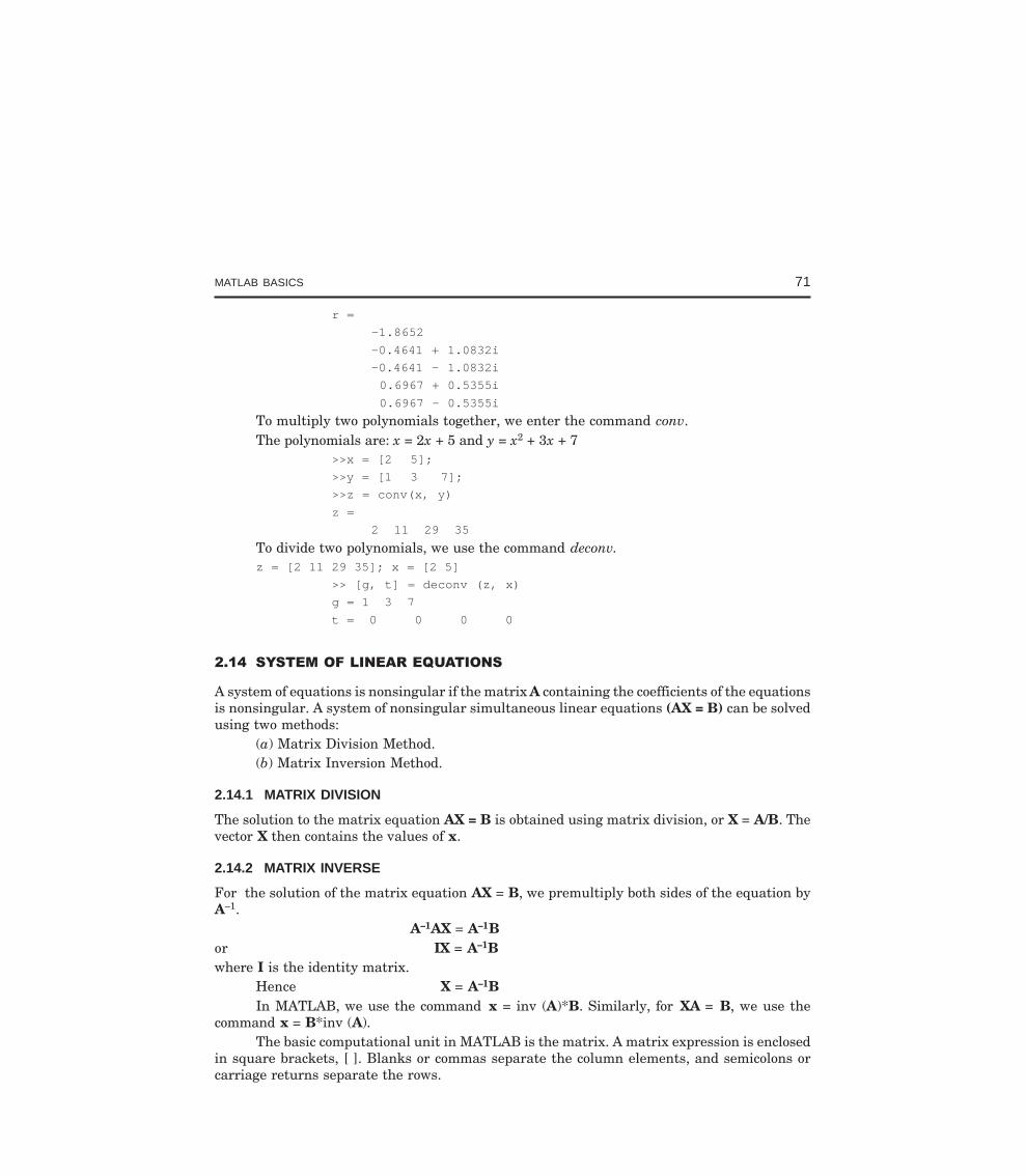
MATLAB BASICS 71
r =
-1.8652
-0.4641 + 1.0832i
-0.4641 - 1.0832i
0.6967 + 0.5355i
0.6967 - 0.5355i
To multiply two polynomials together, we enter the command conv.The polynomials are: x = 2x + 5 and y = x2 + 3x + 7
>>x = [2 5];
>>y = [1 3 7];
>>z = conv(x, y)
z =
2 11 29 35
To divide two polynomials, we use the command deconv.z = [2 11 29 35]; x = [2 5]
>> [g, t] = deconv (z, x)
g = 1 3 7
t = 0 0 0 0
#
A system of equations is nonsingular if the matrix A containing the coefficients of the equationsis nonsingular. A system of nonsingular simultaneous linear equations (AX = B) can be solvedusing two methods:
(a) Matrix Division Method.(b) Matrix Inversion Method.
2.14.1 MATRIX DIVISION
The solution to the matrix equation AX = B is obtained using matrix division, or X = A/B. Thevector X then contains the values of x.
2.14.2 MATRIX INVERSE
For the solution of the matrix equation AX = B, we premultiply both sides of the equation byA–1.
A–1AX = A–1Bor IX = A–1Bwhere I is the identity matrix.
Hence X = A–1BIn MATLAB, we use the command x = inv (A)*B. Similarly, for XA = B, we use the
command x = B*inv (A).The basic computational unit in MATLAB is the matrix. A matrix expression is enclosed
in square brackets, [ ]. Blanks or commas separate the column elements, and semicolons orcarriage returns separate the rows.
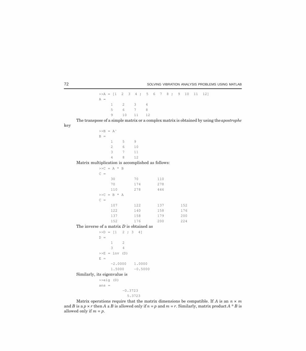
72 SOLVING VIBRATION ANALYSIS PROBLEMS USING MATLAB
>>A = [1 2 3 4 ; 5 6 7 8 ; 9 10 11 12]
A =
1 2 3 4
5 6 7 8
9 10 11 12
The transpose of a simple matrix or a complex matrix is obtained by using the apostrophekey
>>B = A'
B =
1 5 9
2 6 10
3 7 11
4 8 12
Matrix multiplication is accomplished as follows:>>C = A * B
C =
30 70 110
70 174 278
110 278 446
>>C = B * A
C =
107 122 137 152
122 140 158 176
137 158 179 200
152 176 200 224
The inverse of a matrix D is obtained as>>D = [1 2 ; 3 4]
D =
1 2
3 4
>>E = inv (D)
E =
-2.0000 1.0000
1.5000 -0.5000
Similarly, its eigenvalue is>>eig (D)
ans =
-0.3723
5.3723
Matrix operations require that the matrix dimensions be compatible. If A is an n × mand B is a p × r then A ± B is allowed only if n = p and m = r. Similarly, matrix product A * B isallowed only if m = p.
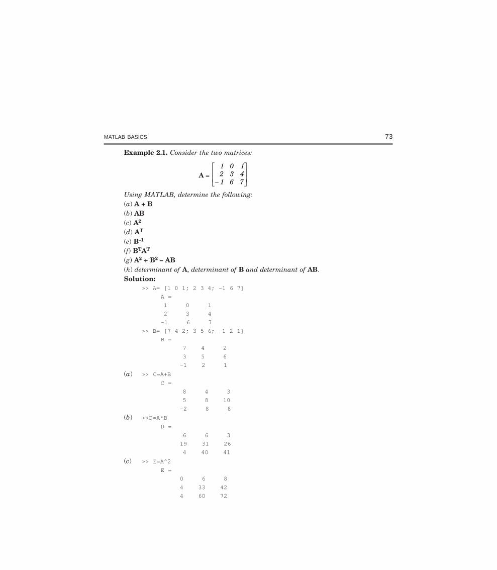
MATLAB BASICS 73
Example 2.1. Consider the two matrices:
A = 1 0 12 3 41 6 7−
L
NMM
O
QPP
Using MATLAB, determine the following:(a) A + B(b) AB(c) A2
(d) AT
(e) B–1
(f) BTAT
(g) A2 + B2 – AB(h) determinant of A, determinant of B and determinant of AB.Solution:
>> A= [1 0 1; 2 3 4; -1 6 7]
A =
1 0 1
2 3 4
-1 6 7
>> B= [7 4 2; 3 5 6; -1 2 1]
B =
7 4 2
3 5 6
-1 2 1
(a) >> C=A+B
C =
8 4 3
5 8 10
-2 8 8
(b) >>D=A*B
D =
6 6 3
19 31 26
4 40 41
(c) >> E=A^2
E =
0 6 8
4 33 42
4 60 72
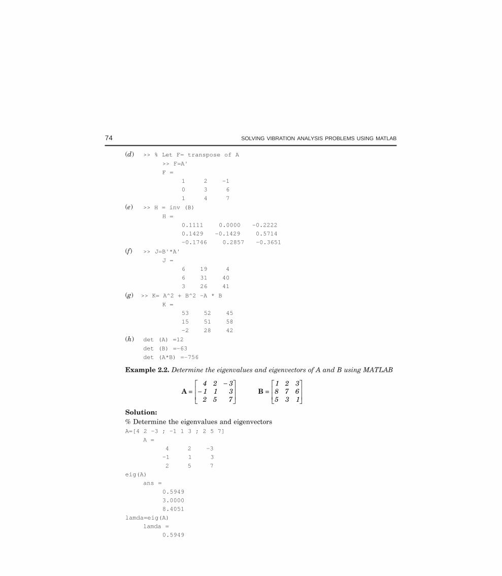
74 SOLVING VIBRATION ANALYSIS PROBLEMS USING MATLAB
(d) >> % Let F= transpose of A
>> F=A'
F =
1 2 -1
0 3 6
1 4 7
(e) >> H = inv (B)
H =
0.1111 0.0000 -0.2222
0.1429 -0.1429 0.5714
-0.1746 0.2857 -0.3651
(f) >> J=B'*A'
J =
6 19 4
6 31 40
3 26 41
(g) >> K= A^2 + B^2 -A * BK =
53 52 45
15 51 58
-2 28 42
(h) det (A) =12
det (B) =-63
det (A*B) =-756
Example 2.2. Determine the eigenvalues and eigenvectors of A and B using MATLAB
A = 4 2 31 1 32 5 7
−−L
NMM
O
QPP B =
1 2 38 7 65 3 1
L
NMM
O
QPP
Solution:% Determine the eigenvalues and eigenvectorsA=[4 2 -3 ; -1 1 3 ; 2 5 7]
A =
4 2 -3
-1 1 3
2 5 7
eig(A)
ans =
0.5949
3.0000
8.4051
lamda=eig(A)
lamda =
0.5949
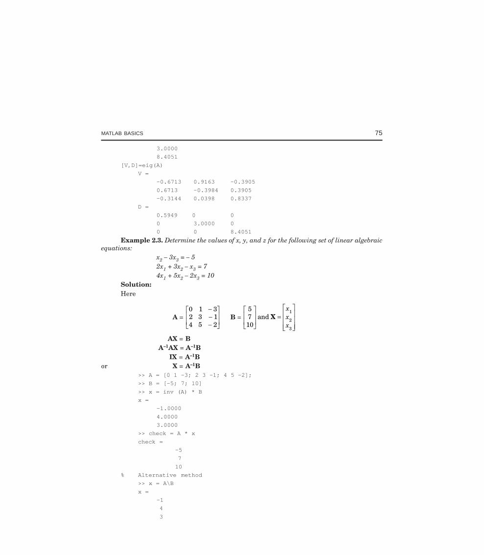
MATLAB BASICS 75
3.0000
8.4051
[V,D]=eig(A)
V =
-0.6713 0.9163 -0.3905
0.6713 -0.3984 0.3905
-0.3144 0.0398 0.8337
D =
0.5949 0 0
0 3.0000 0
0 0 8.4051
Example 2.3. Determine the values of x, y, and z for the following set of linear algebraicequations:
x2 – 3x3 = – 52x1 + 3x2 – x3 = 74x1 + 5x2 – 2x3 = 10
Solution:Here
A = 0 1 32 3 14 5 2
−−−
L
NMM
O
QPP B =
5710
1
2
3
L
NMM
O
QPP =
L
NMMM
O
QPPP
and Xxxx
AX = B A–1AX = A–1B
IX = A–1Bor X = A–1B
>> A = [0 1 -3; 2 3 -1; 4 5 -2];
>> B = [-5; 7; 10]
>> x = inv (A) * B
x =
-1.0000
4.0000
3.0000
>> check = A * x
check =
-5
7
10
% Alternative method
>> x = A\B
x =
-1
4
3
76 SOLVING VIBRATION ANALYSIS PROBLEMS USING MATLAB
A script is a sequence of ordinary statements and functions used at the command prompt level.A script is invoked at the command prompt level by typing the file-name or by using the pulldown menu. Scripts can also invoke other scripts.
The commands in the Command Window cannot be saved and executed again. Also, theCommand Window is not interactive. To overcome these difficulties, the procedure is first tocreate a file with a list of commands, save it, and then run the file. In this way the commandscontained are executed in the order they are listed when the file is run. In addition, as the needarises, one can change or modify the commands in the file, the file can be saved and run again.The files that are used in this fashion are known as script files. Thus, a script file is a text filethat contains a sequence of MATLAB commands. Script file can be edited (corrected and/orchanged) and executed many times.
2.15.1 CREATING AND SAVING A SCRIPT FILE
Any text editor can be used to create script files. In MATLAB script files are created and editedin the Editor/Debugger Window. This window can be opened from the Command Window.From the Command Window, select File, New, and then M-file. Once the window is open, thecommands of the script file are typed line by line. The commands can also be typed in any texteditor or word processor program and then copied and pasted in the Editor/Debugger Window.The second type of M-files is the function file. Function file enables the user to extend the basiclibrary functions by adding one’s own computational procedures. Function M-files are expectedto return one or more results. Script files and function files may include reference to otherMATLAB toolbox routines.
MATLAB function file begins with a header statement of the form:function (name of result or results) = name (argument list)
Before a script file can be executed it must be saved. All script files must be saved withthe extension ‘‘.m’’. MATLAB refers to them as m-files. When using MATLAB M-files editor,the files will automatically be saved with a ‘‘.m’’ extension. If any other text editor is used, thefile must be saved with the ‘‘.m’’ extension, or MATLAB will not be able to find and run thescript file. This is done by choosing Save As… from the File menu, selecting a location, andentering a name for the file. The names of user defined variables, predefined variables, MATLABcommands or functions should not be used to name script files.
2.15.2 RUNNING A SCRIPT FILE
A script file can be executed either by typing its name in the Command Window and thenpressing the Enter key, directly from the Editor Window by clicking on the Run icon. The fileis assumed to be in the current directory, or in the search path.
2.15.3 INPUT TO A SCRIPT FILE
There are three ways of assigning a value to a variable in a script file.1. The variable is defined and assigned value in the script file.2. The variable is defined and assigned value in the Command Window.3. The variable is defined in the script file, but a specified value is entered in the Command
Window when the script file is executed.
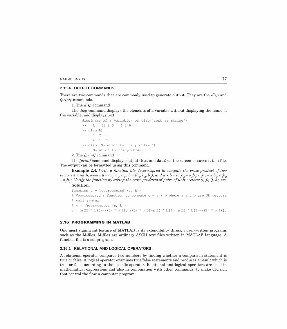
MATLAB BASICS 77
2.15.4 OUTPUT COMMANDS
There are two commands that are commonly used to generate output. They are the disp andfprintf commands.
1. The disp commandThe disp command displays the elements of a variable without displaying the name of
the variable, and displays text.disp(name of a variable) or disp('text as string')
>> A = [1 2 3 ; 4 5 6 ];
>> disp(A)
1 2 3
4 5 6
>> disp('Solution to the problem.')
Solution to the problem.
2. The fprintf commandThe fprintf command displays output (text and data) on the screen or saves it to a file.
The output can be formatted using this command.Example 2.4. Write a function file Veccrossprod to compute the cross product of two
vectors a, and b, where a = (a1, a2, a3), b = (b1, b2, b3), and a × b = (a2b3 – a3b2, a3b1 – a1b3, a1b2– a2b1). Verify the function by taking the cross products of pairs of unit vectors: (i, j), (j, k), etc.
Solution:function c = Veccrossprod (a, b);
% Veccrossprod : function to compute c = a × b where a and b are 3D vectors
% call syntax:
% c = Veccrossprod (a, b);
c = [a(2) * b(3)–a(3) * b(2); a(3) * b(1)–a(1) * b(3); a(1) * b(2)–a(2) * b(1)];
One most significant feature of MATLAB is its extendibility through user-written programssuch as the M-files. M-files are ordinary ASCII text files written in MATLAB language. Afunction file is a subprogram.
2.16.1 RELATIONAL AND LOGICAL OPERATORS
A relational operator compares two numbers by finding whether a comparison statement istrue or false. A logical operator examines true/false statements and produces a result which istrue or false according to the specific operator. Relational and logical operators are used inmathematical expressions and also in combination with other commands, to make decisionthat control the flow a computer program.
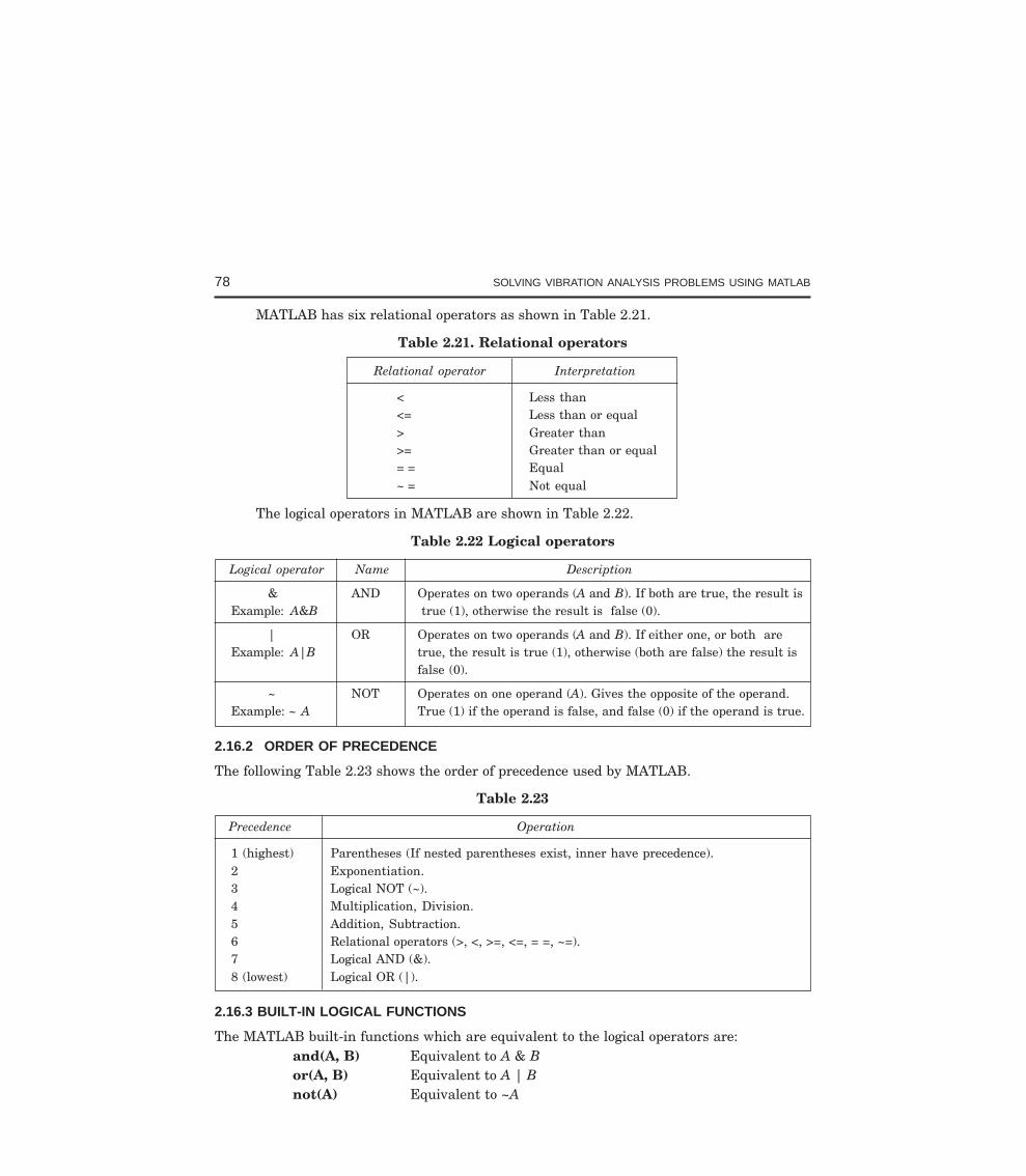
78 SOLVING VIBRATION ANALYSIS PROBLEMS USING MATLAB
MATLAB has six relational operators as shown in Table 2.21.
Table 2.21. Relational operators
Relational operator Interpretation
< Less than<= Less than or equal> Greater than>= Greater than or equal= = Equal~ = Not equal
The logical operators in MATLAB are shown in Table 2.22.
Table 2.22 Logical operators
Logical operator Name Description
& AND Operates on two operands (A and B). If both are true, the result isExample: A&B true (1), otherwise the result is false (0).
| OR Operates on two operands (A and B). If either one, or both areExample: A|B true, the result is true (1), otherwise (both are false) the result is
false (0).
~ NOT Operates on one operand (A). Gives the opposite of the operand.Example: ~ A True (1) if the operand is false, and false (0) if the operand is true.
2.16.2 ORDER OF PRECEDENCE
The following Table 2.23 shows the order of precedence used by MATLAB.
Table 2.23
Precedence Operation
1 (highest) Parentheses (If nested parentheses exist, inner have precedence).2 Exponentiation.3 Logical NOT (~).4 Multiplication, Division.5 Addition, Subtraction.6 Relational operators (>, <, >=, <=, = =, ~=).7 Logical AND (&).8 (lowest) Logical OR (|).
2.16.3 BUILT-IN LOGICAL FUNCTIONS
The MATLAB built-in functions which are equivalent to the logical operators are:and(A, B) Equivalent to A & Bor(A, B) Equivalent to A | Bnot(A) Equivalent to ~A
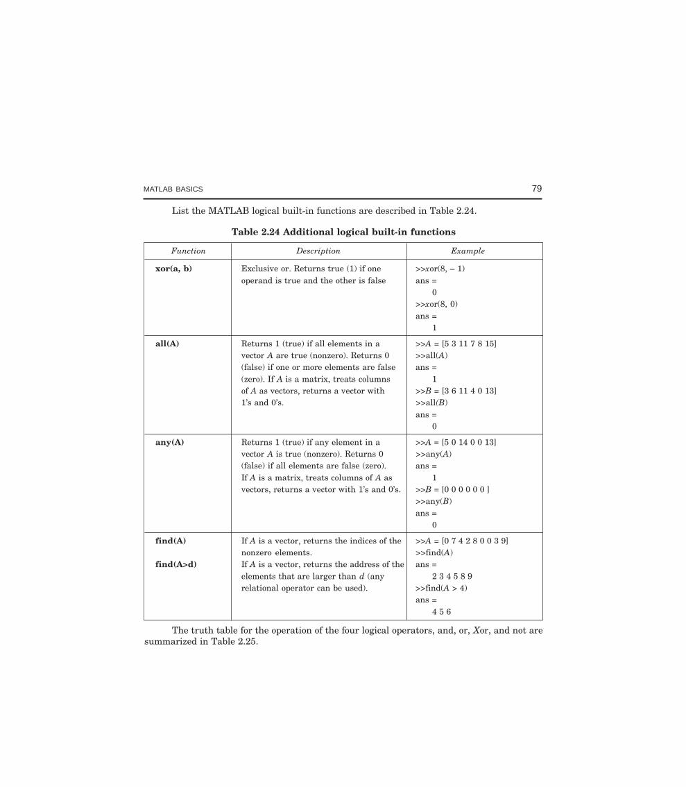
MATLAB BASICS 79
List the MATLAB logical built-in functions are described in Table 2.24.
Table 2.24 Additional logical built-in functions
Function Description Example
xor(a, b) Exclusive or. Returns true (1) if one >>xor(8, – 1)operand is true and the other is false ans =
0>>xor(8, 0)ans =
1
all(A) Returns 1 (true) if all elements in a >>A = [5 3 11 7 8 15]vector A are true (nonzero). Returns 0 >>all(A)(false) if one or more elements are false ans =(zero). If A is a matrix, treats columns 1of A as vectors, returns a vector with >>B = [3 6 11 4 0 13]1’s and 0’s. >>all(B)
ans =0
any(A) Returns 1 (true) if any element in a >>A = [5 0 14 0 0 13]vector A is true (nonzero). Returns 0 >>any(A)(false) if all elements are false (zero). ans =If A is a matrix, treats columns of A as 1vectors, returns a vector with 1’s and 0’s. >>B = [0 0 0 0 0 0 ]
>>any(B)ans =
0
find(A) If A is a vector, returns the indices of the >>A = [0 7 4 2 8 0 0 3 9]nonzero elements. >>find(A)
find(A>d) If A is a vector, returns the address of the ans =elements that are larger than d (any 2 3 4 5 8 9relational operator can be used). >>find(A > 4)
ans =4 5 6
The truth table for the operation of the four logical operators, and, or, Xor, and not aresummarized in Table 2.25.
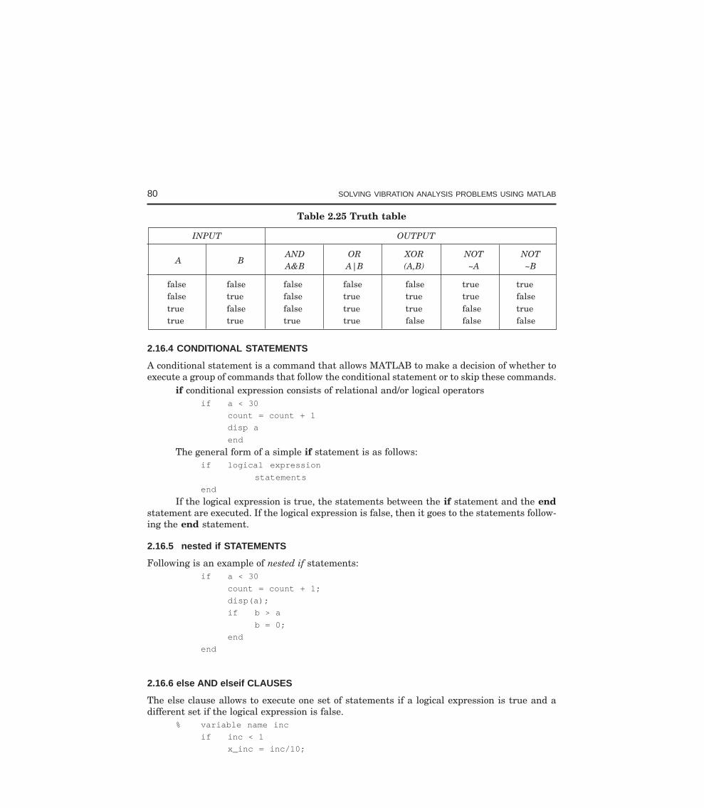
80 SOLVING VIBRATION ANALYSIS PROBLEMS USING MATLAB
Table 2.25 Truth table
INPUT OUTPUT
AND OR XOR NOT NOTA B
A&B A|B (A,B) ~A ~B
false false false false false true truefalse true false true true true falsetrue false false true true false truetrue true true true false false false
2.16.4 CONDITIONAL STATEMENTS
A conditional statement is a command that allows MATLAB to make a decision of whether toexecute a group of commands that follow the conditional statement or to skip these commands.
if conditional expression consists of relational and/or logical operatorsif a < 30
count = count + 1
disp a
end
The general form of a simple if statement is as follows:if logical expression
statements
end
If the logical expression is true, the statements between the if statement and the endstatement are executed. If the logical expression is false, then it goes to the statements follow-ing the end statement.
2.16.5 nested if STATEMENTS
Following is an example of nested if statements:if a < 30
count = count + 1;
disp(a);
if b > a
b = 0;
end
end
2.16.6 else AND elseif CLAUSES
The else clause allows to execute one set of statements if a logical expression is true and adifferent set if the logical expression is false.
% variable name inc
if inc < 1
x_inc = inc/10;
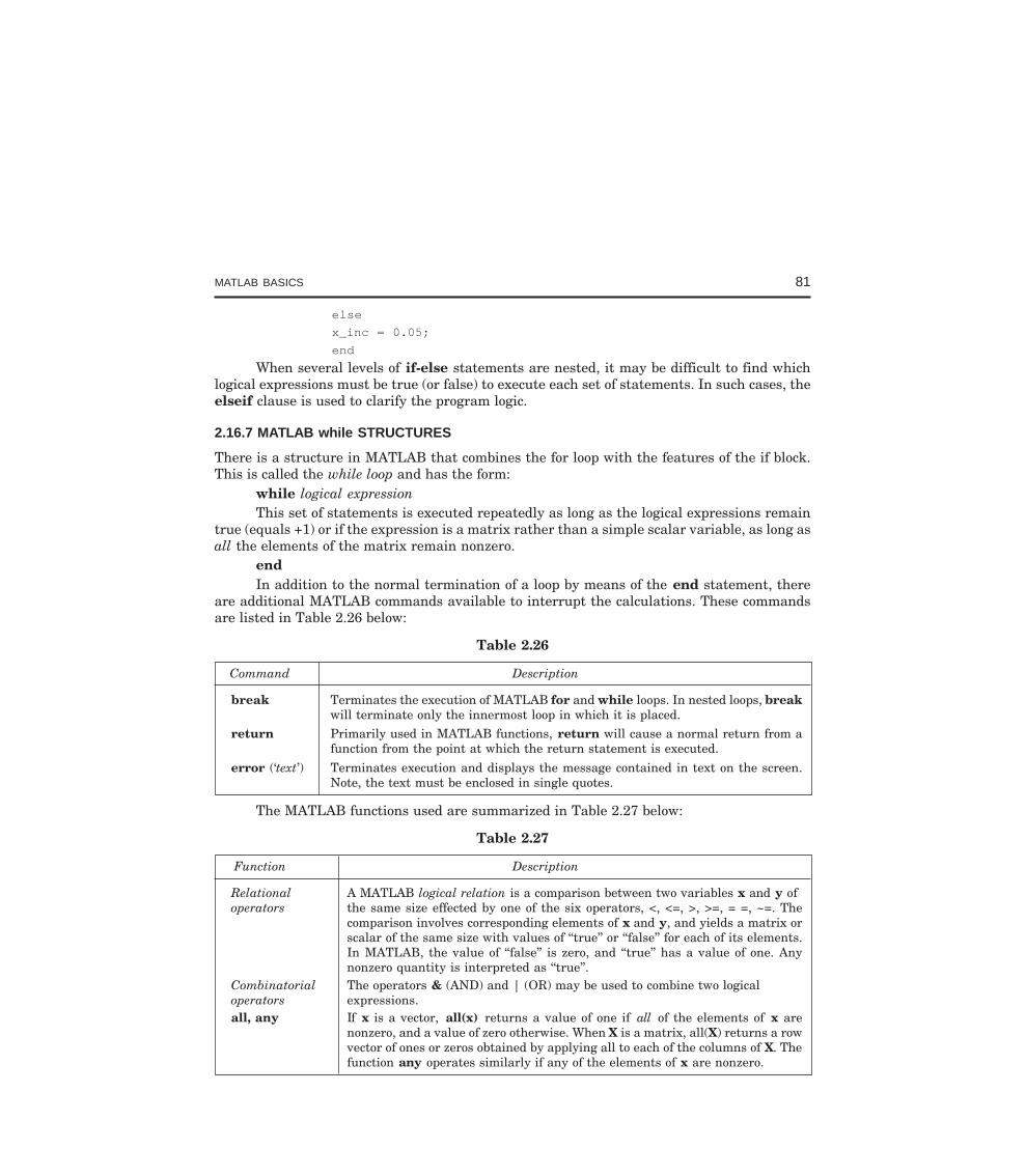
MATLAB BASICS 81
else
x_inc = 0.05;
end
When several levels of if-else statements are nested, it may be difficult to find whichlogical expressions must be true (or false) to execute each set of statements. In such cases, theelseif clause is used to clarify the program logic.
2.16.7 MATLAB while STRUCTURES
There is a structure in MATLAB that combines the for loop with the features of the if block.This is called the while loop and has the form:
while logical expressionThis set of statements is executed repeatedly as long as the logical expressions remain
true (equals +1) or if the expression is a matrix rather than a simple scalar variable, as long asall the elements of the matrix remain nonzero.
endIn addition to the normal termination of a loop by means of the end statement, there
are additional MATLAB commands available to interrupt the calculations. These commandsare listed in Table 2.26 below:
Table 2.26
Command Description
break Terminates the execution of MATLAB for and while loops. In nested loops, breakwill terminate only the innermost loop in which it is placed.
return Primarily used in MATLAB functions, return will cause a normal return from afunction from the point at which the return statement is executed.
error (‘text’) Terminates execution and displays the message contained in text on the screen.Note, the text must be enclosed in single quotes.
The MATLAB functions used are summarized in Table 2.27 below:
Table 2.27
Function Description
Relational A MATLAB logical relation is a comparison between two variables x and y ofoperators the same size effected by one of the six operators, <, <=, >, >=, = =, ~=. The
comparison involves corresponding elements of x and y, and yields a matrix orscalar of the same size with values of ‘‘true’’ or ‘‘false’’ for each of its elements.In MATLAB, the value of ‘‘false’’ is zero, and ‘‘true’’ has a value of one. Anynonzero quantity is interpreted as ‘‘true’’.
Combinatorial The operators & (AND) and | (OR) may be used to combine two logicaloperators expressions.all, any If x is a vector, all(x) returns a value of one if all of the elements of x are
nonzero, and a value of zero otherwise. When X is a matrix, all(X) returns a rowvector of ones or zeros obtained by applying all to each of the columns of X. Thefunction any operates similarly if any of the elements of x are nonzero.
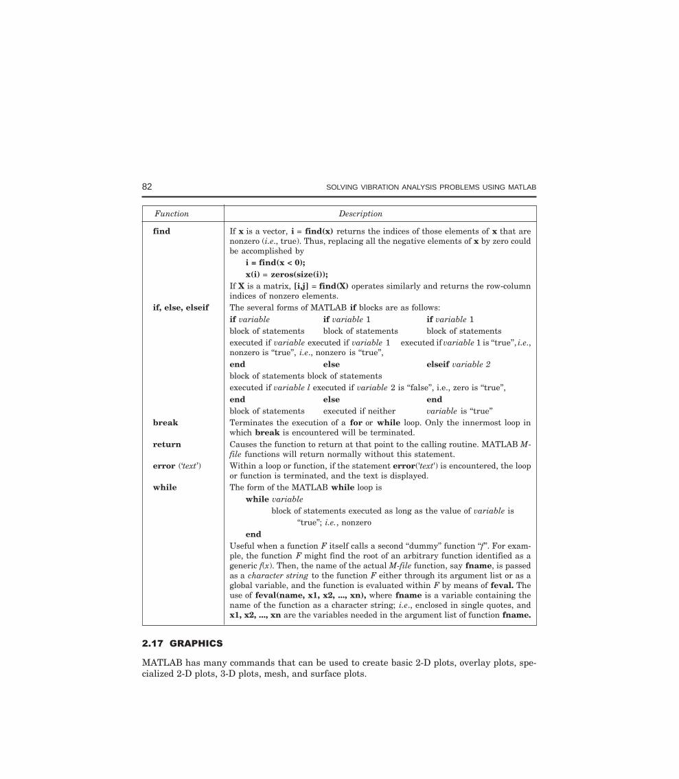
82 SOLVING VIBRATION ANALYSIS PROBLEMS USING MATLAB
Function Description
find If x is a vector, i = find(x) returns the indices of those elements of x that arenonzero (i.e., true). Thus, replacing all the negative elements of x by zero couldbe accomplished by
i = find(x < 0);x(i) = zeros(size(i));
If X is a matrix, [i,j] = find(X) operates similarly and returns the row-columnindices of nonzero elements.
if, else, elseif The several forms of MATLAB if blocks are as follows:if variable if variable 1 if variable 1block of statements block of statements block of statementsexecuted if variable executed if variable 1 executed if variable 1 is ‘‘true’’, i.e.,nonzero is ‘‘true’’, i.e., nonzero is ‘‘true’’,end else elseif variable 2block of statements block of statementsexecuted if variable l executed if variable 2 is ‘‘false’’, i.e., zero is ‘‘true’’,end else endblock of statements executed if neither variable is ‘‘true’’
break Terminates the execution of a for or while loop. Only the innermost loop inwhich break is encountered will be terminated.
return Causes the function to return at that point to the calling routine. MATLAB M-file functions will return normally without this statement.
error (‘text’) Within a loop or function, if the statement error('text') is encountered, the loopor function is terminated, and the text is displayed.
while The form of the MATLAB while loop iswhile variable
block of statements executed as long as the value of variable is‘‘true’’; i.e., nonzero
endUseful when a function F itself calls a second ‘‘dummy’’ function ‘‘f’’. For exam-ple, the function F might find the root of an arbitrary function identified as ageneric f(x). Then, the name of the actual M-file function, say fname, is passedas a character string to the function F either through its argument list or as aglobal variable, and the function is evaluated within F by means of feval. Theuse of feval(name, x1, x2, ..., xn), where fname is a variable containing thename of the function as a character string; i.e., enclosed in single quotes, andx1, x2, ..., xn are the variables needed in the argument list of function fname.
MATLAB has many commands that can be used to create basic 2-D plots, overlay plots, spe-cialized 2-D plots, 3-D plots, mesh, and surface plots.
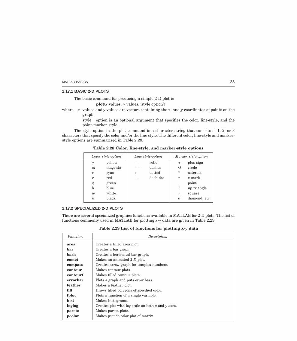
MATLAB BASICS 83
2.17.1 BASIC 2-D PLOTS
The basic command for producing a simple 2-D plot isplot(x values, y values, ‘style option’)
where x values and y values are vectors containing the x- and y-coordinates of points on thegraph.style option is an optional argument that specifies the color, line-style, and thepoint-marker style.
The style option in the plot command is a character string that consists of 1, 2, or 3characters that specify the color and/or the line style. The different color, line-style and marker-style options are summarized in Table 2.28.
Table 2.28 Color, line-style, and marker-style options
Color style-option Line style-option Marker style-option
y yellow – solid + plus signm magenta – – dashes O circlec cyan : dotted * asteriskr red –. dash-dot x x-markg green . pointb blue ^ up trianglew white s squarek black d diamond, etc.
2.17.2 SPECIALIZED 2-D PLOTS
There are several specialized graphics functions available in MATLAB for 2-D plots. The list offunctions commonly used in MATLAB for plotting x-y data are given in Table 2.29.
Table 2.29 List of functions for plotting x-y data
Function Description
area Creates a filled area plot.bar Creates a bar graph.barh Creates a horizontal bar graph.comet Makes an animated 2-D plot.compass Creates arrow graph for complex numbers.contour Makes contour plots.contourf Makes filled contour plots.errorbar Plots a graph and puts error bars.feather Makes a feather plot.fill Draws filled polygons of specified color.fplot Plots a function of a single variable.hist Makes histograms.loglog Creates plot with log scale on both x and y axes.pareto Makes pareto plots.pcolor Makes pseudo color plot of matrix.
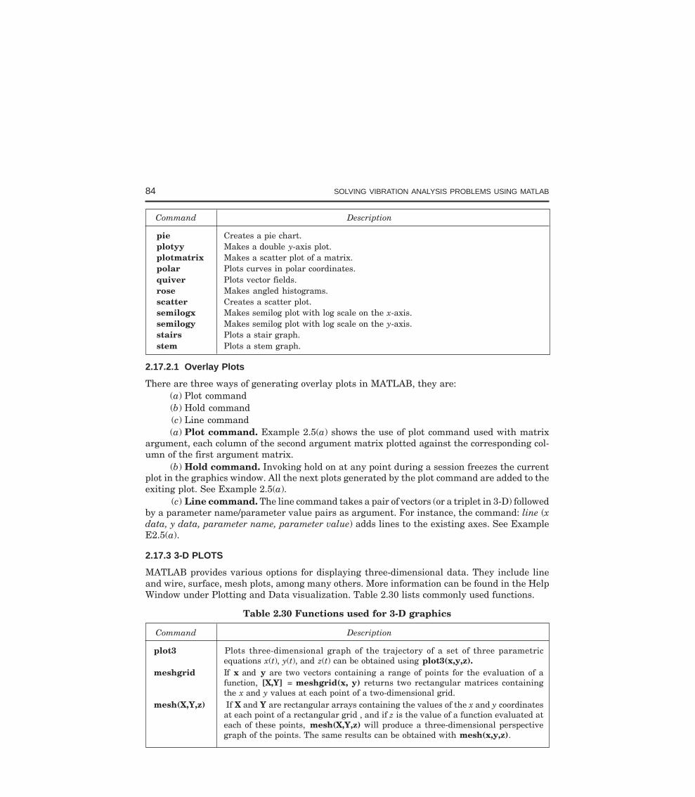
84 SOLVING VIBRATION ANALYSIS PROBLEMS USING MATLAB
Command Description
pie Creates a pie chart.plotyy Makes a double y-axis plot.plotmatrix Makes a scatter plot of a matrix.polar Plots curves in polar coordinates.quiver Plots vector fields.rose Makes angled histograms.scatter Creates a scatter plot.semilogx Makes semilog plot with log scale on the x-axis.semilogy Makes semilog plot with log scale on the y-axis.stairs Plots a stair graph.stem Plots a stem graph.
2.17.2.1 Overlay Plots
There are three ways of generating overlay plots in MATLAB, they are:(a) Plot command(b) Hold command(c) Line command(a) Plot command. Example 2.5(a) shows the use of plot command used with matrix
argument, each column of the second argument matrix plotted against the corresponding col-umn of the first argument matrix.
(b) Hold command. Invoking hold on at any point during a session freezes the currentplot in the graphics window. All the next plots generated by the plot command are added to theexiting plot. See Example 2.5(a).
(c) Line command. The line command takes a pair of vectors (or a triplet in 3-D) followedby a parameter name/parameter value pairs as argument. For instance, the command: line (xdata, y data, parameter name, parameter value) adds lines to the existing axes. See ExampleE2.5(a).
2.17.3 3-D PLOTS
MATLAB provides various options for displaying three-dimensional data. They include lineand wire, surface, mesh plots, among many others. More information can be found in the HelpWindow under Plotting and Data visualization. Table 2.30 lists commonly used functions.
Table 2.30 Functions used for 3-D graphics
Command Description
plot3 Plots three-dimensional graph of the trajectory of a set of three parametricequations x(t), y(t), and z(t) can be obtained using plot3(x,y,z).
meshgrid If x and y are two vectors containing a range of points for the evaluation of afunction, [X,Y] = meshgrid(x, y) returns two rectangular matrices containingthe x and y values at each point of a two-dimensional grid.
mesh(X,Y,z) If X and Y are rectangular arrays containing the values of the x and y coordinatesat each point of a rectangular grid , and if z is the value of a function evaluated ateach of these points, mesh(X,Y,z) will produce a three-dimensional perspectivegraph of the points. The same results can be obtained with mesh(x,y,z).
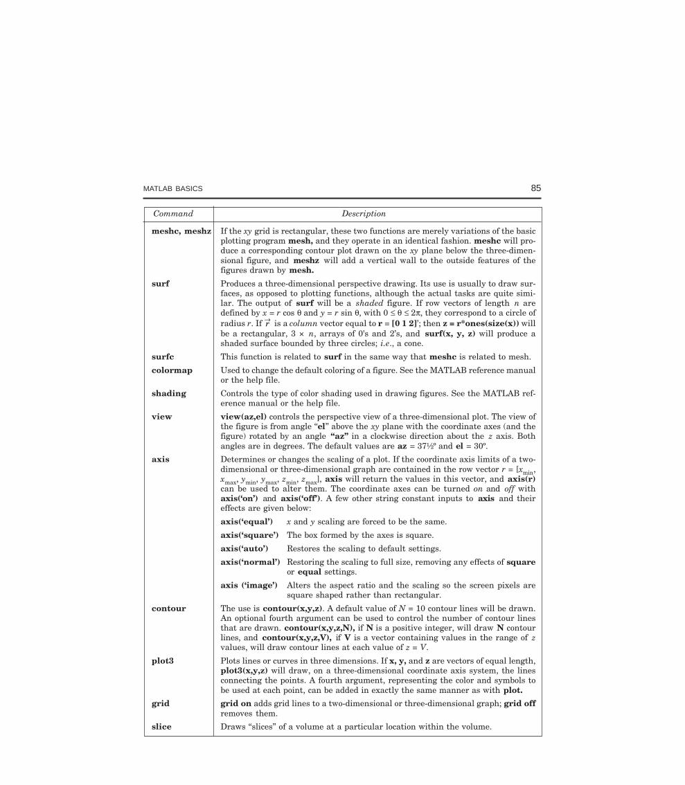
MATLAB BASICS 85
Command Description
meshc, meshz If the xy grid is rectangular, these two functions are merely variations of the basicplotting program mesh, and they operate in an identical fashion. meshc will pro-duce a corresponding contour plot drawn on the xy plane below the three-dimen-sional figure, and meshz will add a vertical wall to the outside features of thefigures drawn by mesh.
surf Produces a three-dimensional perspective drawing. Its use is usually to draw sur-faces, as opposed to plotting functions, although the actual tasks are quite simi-lar. The output of surf will be a shaded figure. If row vectors of length n aredefined by x = r cos θ and y = r sin θ, with 0 ≤ θ ≤ 2π, they correspond to a circle ofradius r. If r→ is a column vector equal to r = [0 1 2]’; then z = r*ones(size(x)) willbe a rectangular, 3 × n, arrays of 0's and 2’s, and surf(x, y, z) will produce ashaded surface bounded by three circles; i.e., a cone.
surfc This function is related to surf in the same way that meshc is related to mesh.
colormap Used to change the default coloring of a figure. See the MATLAB reference manualor the help file.
shading Controls the type of color shading used in drawing figures. See the MATLAB ref-erence manual or the help file.
view view(az,el) controls the perspective view of a three-dimensional plot. The view ofthe figure is from angle ‘‘el’’ above the xy plane with the coordinate axes (and thefigure) rotated by an angle ‘‘az’’ in a clockwise direction about the z axis. Bothangles are in degrees. The default values are az = 37½º and el = 30º.
axis Determines or changes the scaling of a plot. If the coordinate axis limits of a two-dimensional or three-dimensional graph are contained in the row vector r = [xmin,xmax, ymin, ymax, zmin, zmax], axis will return the values in this vector, and axis(r)can be used to alter them. The coordinate axes can be turned on and off withaxis(‘on’) and axis(‘off’). A few other string constant inputs to axis and theireffects are given below:
axis(‘equal’) x and y scaling are forced to be the same.
axis(‘square’) The box formed by the axes is square.
axis(‘auto’) Restores the scaling to default settings.
axis(‘normal’) Restoring the scaling to full size, removing any effects of squareor equal settings.
axis (‘image’) Alters the aspect ratio and the scaling so the screen pixels aresquare shaped rather than rectangular.
contour The use is contour(x,y,z). A default value of N = 10 contour lines will be drawn.An optional fourth argument can be used to control the number of contour linesthat are drawn. contour(x,y,z,N), if N is a positive integer, will draw N contourlines, and contour(x,y,z,V), if V is a vector containing values in the range of zvalues, will draw contour lines at each value of z = V.
plot3 Plots lines or curves in three dimensions. If x, y, and z are vectors of equal length,plot3(x,y,z) will draw, on a three-dimensional coordinate axis system, the linesconnecting the points. A fourth argument, representing the color and symbols tobe used at each point, can be added in exactly the same manner as with plot.
grid grid on adds grid lines to a two-dimensional or three-dimensional graph; grid offremoves them.
slice Draws ‘‘slices’’ of a volume at a particular location within the volume.
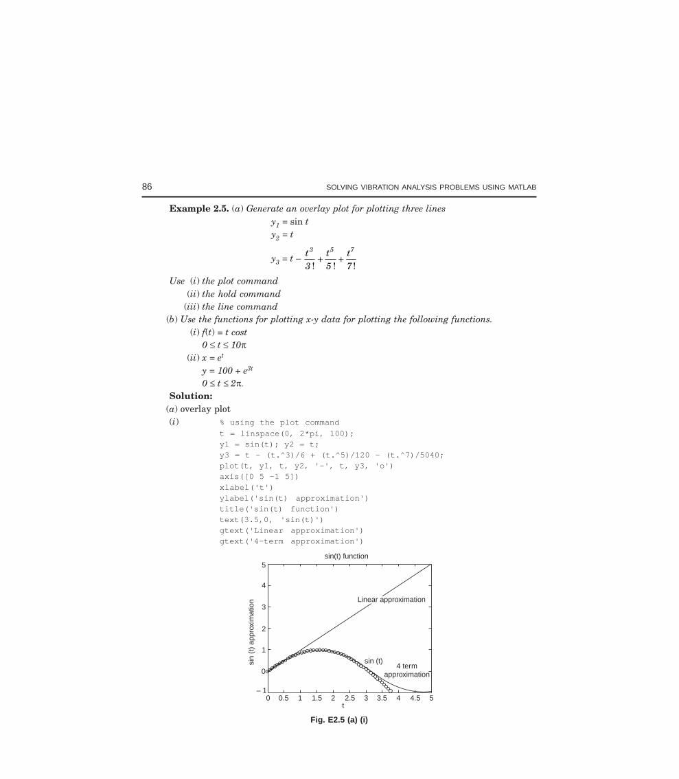
86 SOLVING VIBRATION ANALYSIS PROBLEMS USING MATLAB
Example 2.5. (a) Generate an overlay plot for plotting three linesy1 = sin ty2 = t
y3 = t – t3
t5
t7
3 5 7
! ! !+ +
Use (i) the plot command(ii) the hold command
(iii) the line command(b) Use the functions for plotting x-y data for plotting the following functions.
(i) f(t) = t cost0 ≤ t ≤ 10π
(ii) x = et
y = 100 + e3t
0 ≤ t ≤ 2π.Solution:
(a) overlay plot(i) % using the plot command
t = linspace(0, 2*pi, 100);y1 = sin(t); y2 = t;y3 = t – (t.^3)/6 + (t.^5)/120 - (t.^7)/5040;plot(t, y1, t, y2, '-', t, y3, 'o')axis([0 5 -1 5])
xlabel('t')ylabel('sin(t) approximation')title('sin(t) function')text(3.5,0, 'sin(t)')gtext('Linear approximation')gtext('4-term approximation')
5sin(t) function
4
3
2
1
0
– 10 0.5 1 1.5 2 2.5 3 3.5 4 4.5 5
4 termapproximation
sin (t)
t
sin
(t)
appr
oxim
atio
n Linear approximationLinear approximation
Fig. E2.5 (a) (i)
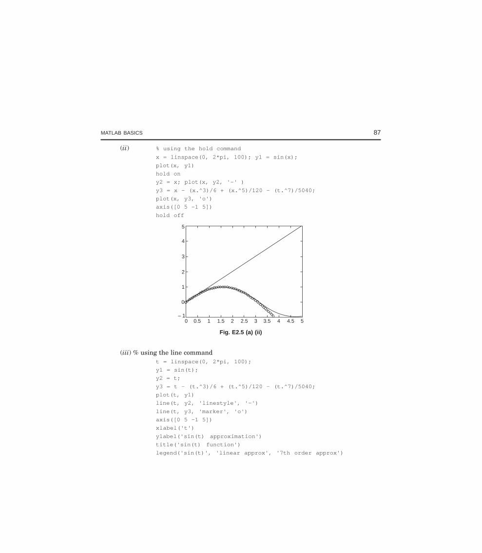
MATLAB BASICS 87
(ii) % using the hold command
x = linspace(0, 2*pi, 100); y1 = sin(x);
plot(x, y1)
hold on
y2 = x; plot(x, y2, '-' )
y3 = x - (x.^3)/6 + (x.^5)/120 - (t.^7)/5040;
plot(x, y3, 'o')
axis([0 5 -1 5])
hold off
5
4
3
2
1
0
– 10 0.5 1 1.5 2 2.5 3 3.5 4 4.5 5
Fig. E2.5 (a) (ii)
(iii) % using the line commandt = linspace(0, 2*pi, 100);
y1 = sin(t);
y2 = t;
y3 = t - (t.^3)/6 + (t.^5)/120 - (t.^7)/5040;
plot(t, y1)
line(t, y2, 'linestyle', '-')
line(t, y3, 'marker', 'o')
axis([0 5 -1 5])
xlabel('t')
ylabel('sin(t) approximation')
title('sin(t) function')
legend('sin(t)', 'linear approx', '7th order approx')
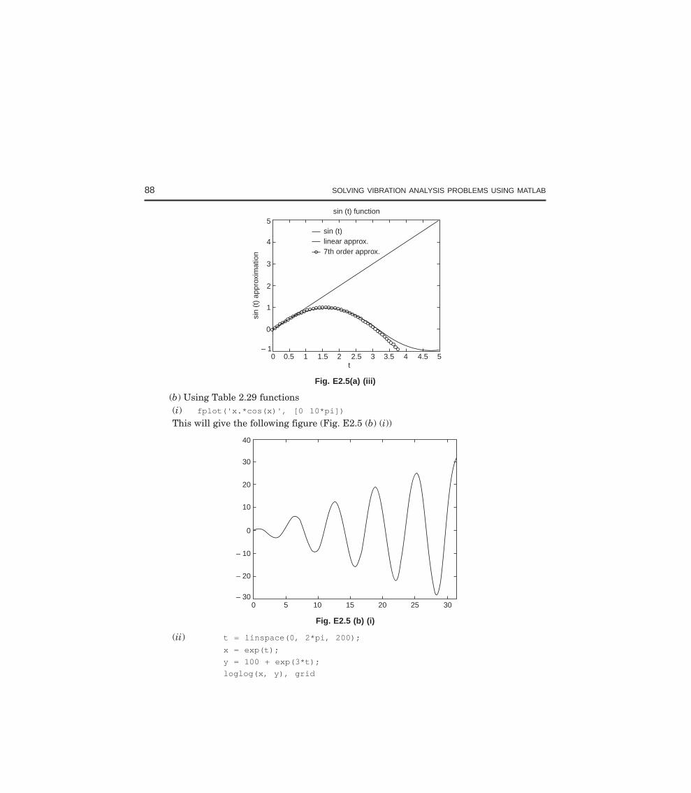
88 SOLVING VIBRATION ANALYSIS PROBLEMS USING MATLAB
5
4
3
2
1
0
– 10 0.5 1 1.5 2 2.5 3 3.5 4 4.5 5
t
sin
(t)
appr
oxim
atio
n
sin (t) function
sin (t)linear approx.7th order approx.
Fig. E2.5(a) (iii)
(b) Using Table 2.29 functions(i) fplot('x.*cos(x)', [0 10*pi])
This will give the following figure (Fig. E2.5 (b) (i))
40
30
20
10
0
– 10
– 20
– 300 5 10 15 20 25 30
Fig. E2.5 (b) (i)
(ii) t = linspace(0, 2*pi, 200);
x = exp(t);
y = 100 + exp(3*t);
loglog(x, y), grid
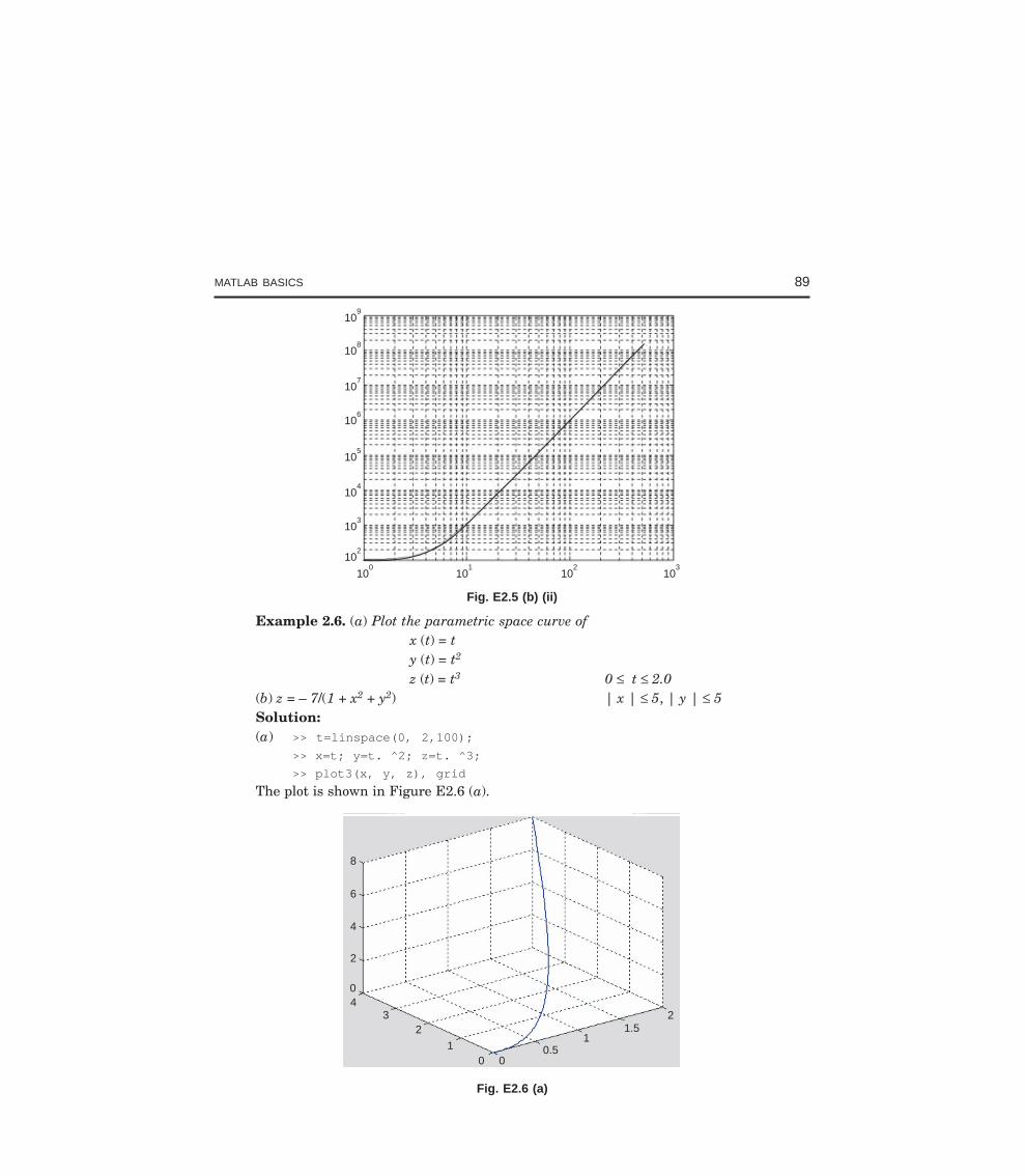
MATLAB BASICS 89
109
108
107
106
105
104
103
102
100
101
102
103
Fig. E2.5 (b) (ii)
Example 2.6. (a) Plot the parametric space curve ofx (t) = ty (t) = t2
z (t) = t3 0 ≤ t ≤ 2.0(b) z = – 7/(1 + x2 + y2) | x | ≤ 5, | y | ≤ 5Solution:(a) >> t=linspace(0, 2,100);
>> x=t; y=t. ^2; z=t. ^3;
>> plot3(x, y, z), grid
The plot is shown in Figure E2.6 (a).
1.51.522
110.50.5
000011
2233
4400
22
44
66
88
Fig. E2.6 (a)
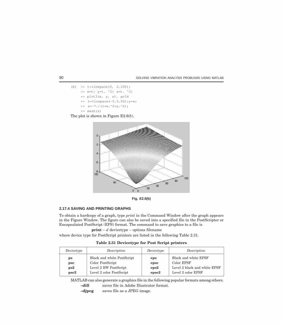
90 SOLVING VIBRATION ANALYSIS PROBLEMS USING MATLAB
(b) >> t=linspace(0, 2,100);
>> x=t; y=t. ^2; z=t. ^3;
>> plot3(x, y, z), grid
>> t=linspace(-5,5,50);y=x;
>> z=-7./(1+x.^2+y.^2);
>> mesh(z)
The plot is shown in Figure E2.6(b).
Fig. E2.6(b)
2.17.4 SAVING AND PRINTING GRAPHS
To obtain a hardcopy of a graph, type print in the Command Window after the graph appearsin the Figure Window. The figure can also be saved into a specified file in the PostScripter orEncapsulated PostScript (EPS) format. The command to save graphics to a file is
print – d devicetype – options filenamewhere device type for PostScript printers are listed in the following Table 2.31.
Table 2.31 Devicetype for Post Script printers
Devicetype Description Devicetype Description
ps Black and white PostScript eps Black and white EPSFpsc Color PostScript epsc Color EPSFps2 Level 2 BW PostScript eps2 Level 2 black and white EPSFpsc2 Level 2 color PostScript epsc2 Level 2 color EPSF
MATLAB can also generate a graphics file in the following popular formats among others.–dill saves file in Adobe Illustrator format.–djpeg saves file as a JPEG image.
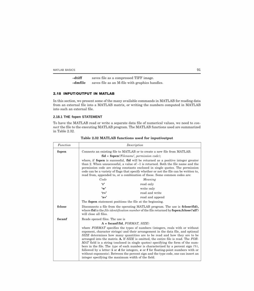
MATLAB BASICS 91
–dtiff saves file as a compressed TIFF image.–dmfile saves file as an M-file with graphics handles.
In this section, we present some of the many available commands in MATLAB for reading datafrom an external file into a MATLAB matrix, or writing the numbers computed in MATLABinto such an external file.
2.18.1 THE fopen STATEMENT
To have the MATLAB read or write a separate data file of numerical values, we need to con-nect the file to the executing MATLAB program. The MATLAB functions used are summarizedin Table 2.32.
Table 2.32 MATLAB functions used for input/output
Function Description
fopen Connects an existing file to MATLAB or to create a new file from MATLAB.fid = fopen(‘Filename’, permission code);
where, if fopen is successful, fid will be returned as a positive integer greaterthan 2. When unsuccessful, a value of –1 is returned. Both the file name and thepermission code are string constants enclosed in single quotes. The permissioncode can be a variety of flags that specify whether or not the file can be written to,read from, appended to, or a combination of these. Some common codes are:
Code Meaning
‘r’ read only‘w’ write only‘r+’ read and write‘a+’ read and append
The fopen statement positions the file at the beginning.
fclose Disconnects a file from the operating MATLAB program. The use is fclose(fid),where fid is the file identification number of the file returned by fopen.fclose(‘all’)will close all files.
fscanf Reads opened files. The use isA = fscanf(fid, FORMAT, SIZE)
where FORMAT specifies the types of numbers (integers, reals with or withoutexponent, character strings) and their arrangement in the data file, and optionalSIZE determines how many quantities are to be read and how they are to bearranged into the matrix A. If SIZE is omitted, the entire file is read. The FOR-MAT field is a string (enclosed in single quotes) specifying the form of the num-bers in the file. The type of each number is characterized by a percent sign (%),followed by a letter (i or d for integers, e or f for floating-point numbers with orwithout exponents). Between the percent sign and the type code, one can insert aninteger specifying the maximum width of the field.
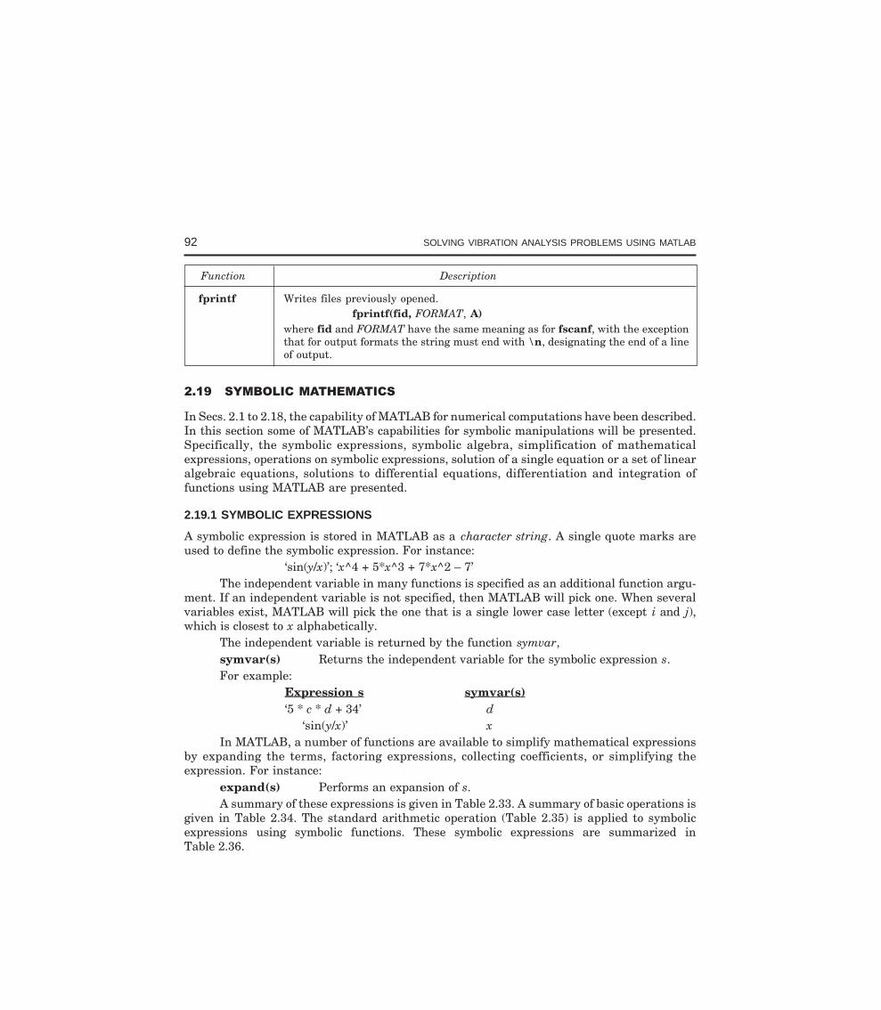
92 SOLVING VIBRATION ANALYSIS PROBLEMS USING MATLAB
Function Description
fprintf Writes files previously opened.fprintf(fid, FORMAT, A)
where fid and FORMAT have the same meaning as for fscanf, with the exceptionthat for output formats the string must end with \n, designating the end of a lineof output.
In Secs. 2.1 to 2.18, the capability of MATLAB for numerical computations have been described.In this section some of MATLAB’s capabilities for symbolic manipulations will be presented.Specifically, the symbolic expressions, symbolic algebra, simplification of mathematicalexpressions, operations on symbolic expressions, solution of a single equation or a set of linearalgebraic equations, solutions to differential equations, differentiation and integration offunctions using MATLAB are presented.
2.19.1 SYMBOLIC EXPRESSIONS
A symbolic expression is stored in MATLAB as a character string. A single quote marks areused to define the symbolic expression. For instance:
‘sin(y/x)’; ‘x^4 + 5*x^3 + 7*x^2 – 7’The independent variable in many functions is specified as an additional function argu-
ment. If an independent variable is not specified, then MATLAB will pick one. When severalvariables exist, MATLAB will pick the one that is a single lower case letter (except i and j),which is closest to x alphabetically.
The independent variable is returned by the function symvar,symvar(s) Returns the independent variable for the symbolic expression s.For example:
Expression s symvar(s)‘5 * c * d + 34’ d
‘sin(y/x)’ xIn MATLAB, a number of functions are available to simplify mathematical expressions
by expanding the terms, factoring expressions, collecting coefficients, or simplifying theexpression. For instance:
expand(s) Performs an expansion of s.A summary of these expressions is given in Table 2.33. A summary of basic operations is
given in Table 2.34. The standard arithmetic operation (Table 2.35) is applied to symbolicexpressions using symbolic functions. These symbolic expressions are summarized inTable 2.36.
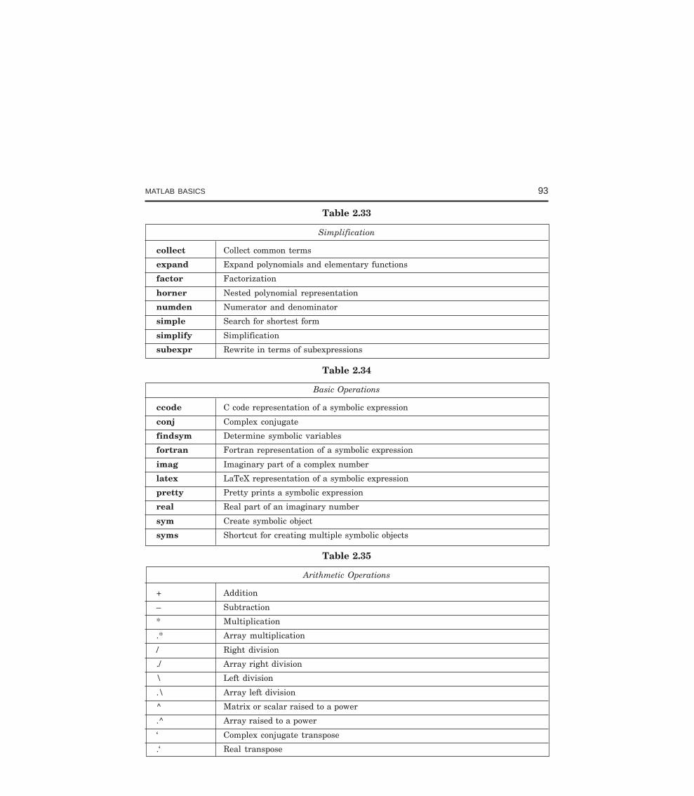
MATLAB BASICS 93
Table 2.33
Simplification
collect Collect common terms
expand Expand polynomials and elementary functions
factor Factorization
horner Nested polynomial representation
numden Numerator and denominator
simple Search for shortest form
simplify Simplification
subexpr Rewrite in terms of subexpressions
Table 2.34
Basic Operations
ccode C code representation of a symbolic expression
conj Complex conjugate
findsym Determine symbolic variables
fortran Fortran representation of a symbolic expression
imag Imaginary part of a complex number
latex LaTeX representation of a symbolic expression
pretty Pretty prints a symbolic expression
real Real part of an imaginary number
sym Create symbolic object
syms Shortcut for creating multiple symbolic objects
Table 2.35
Arithmetic Operations
+ Addition
– Subtraction
* Multiplication
.* Array multiplication
/ Right division
./ Array right division
\ Left division
.\ Array left division
^ Matrix or scalar raised to a power
.^ Array raised to a power
‘ Complex conjugate transpose
.‘ Real transpose
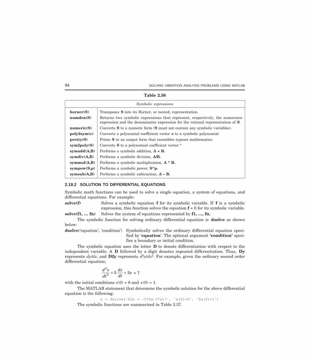
94 SOLVING VIBRATION ANALYSIS PROBLEMS USING MATLAB
Table 2.36
Symbolic expressions
horner(S) Transposes S into its Horner, or nested, representation.
numden(S) Returns two symbolic expressions that represent, respectively, the numeratorexpression and the denominator expression for the rational representation of S.
numeric(S) Converts S to a numeric form (S must not contain any symbolic variables).
poly2sym(c) Converts a polynomial coefficient vector c to a symbolic polynomial.
pretty(S) Prints S in an output form that resembles typeset mathematics.
sym2poly(S) Converts S to a polynomial coefficient vector.*
symadd(A,B) Performs a symbolic addition, A + B.symdiv(A,B) Performs a symbolic division, A/B.symmul(A,B) Performs a symbolic multiplication, A * B.sympow(S,p) Performs a symbolic power, S^p.symsub(A,B) Performs a symbolic subtraction, A – B.
2.19.2 SOLUTION TO DIFFERENTIAL EQUATIONS
Symbolic math functions can be used to solve a single equation, a system of equations, anddifferential equations. For example:solve(f) Solves a symbolic equation f for its symbolic variable. If f is a symbolic
expression, this function solves the equation f = 0 for its symbolic variable.solve(f1, … fn) Solves the system of equations represented by f1, …, fn.
The symbolic function for solving ordinary differential equation is dsolve as shownbelow:dsolve(‘equation’, ‘condition’) Symbolically solves the ordinary differential equation speci-
fied by ‘equation’. The optional argument ‘condition’ speci-fies a boundary or initial condition.
The symbolic equation uses the letter D to denote differentiation with respect to theindependent variable. A D followed by a digit denotes repeated differentiation. Thus, Dyrepresents dy/dx, and D2y represents d2y/dx2. For example, given the ordinary second orderdifferential equation;
d x
dt
dxdt
x2
2 5 3+ + = 7
with the initial conditions x(0) = 0 and x (0) = 1.The MATLAB statement that determine the symbolic solution for the above differential
equation is the following:x = dsolve('D2x = -5*Dx-3*x+7', 'x(0)=0', 'Dx(0)=1')
The symbolic functions are summarized in Table 2.37.
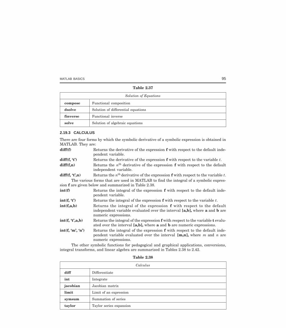
MATLAB BASICS 95
Table 2.37
Solution of Equations
compose Functional composition
dsolve Solution of differential equations
finverse Functional inverse
solve Solution of algebraic equations
2.19.3 CALCULUS
There are four forms by which the symbolic derivative of a symbolic expression is obtained inMATLAB. They are:diff(f) Returns the derivative of the expression f with respect to the default inde-
pendent variable.diff(f, ‘t’) Returns the derivative of the expression f with respect to the variable t.diff(f,n) Returns the nth derivative of the expression f with respect to the default
independent variable.diff(f, ‘t’,n) Returns the nth derivative of the expression f with respect to the variable t.
The various forms that are used in MATLAB to find the integral of a symbolic expres-sion f are given below and summarized in Table 2.38.int(f) Returns the integral of the expression f with respect to the default inde-
pendent variable.int(f, ‘t’) Returns the integral of the expression f with respect to the variable t.int(f,a,b) Returns the integral of the expression f with respect to the default
independent variable evaluated over the interval [a,b], where a and b arenumeric expressions.
int(f, ‘t’,a,b) Returns the integral of the expression f with respect to the variable t evalu-ated over the interval [a,b], where a and b are numeric expressions.
int(f, ‘m’, ‘n’) Returns the integral of the expression f with respect to the default inde-pendent variable evaluated over the interval [m,n], where m and n arenumeric expressions.
The other symbolic functions for pedagogical and graphical applications, conversions,integral transforms, and linear algebra are summarized in Tables 2.38 to 2.42.
Table 2.38
Calculus
diff Differentiate
int Integrate
jacobian Jacobian matrix
limit Limit of an expression
symsum Summation of series
taylor Taylor series expansion
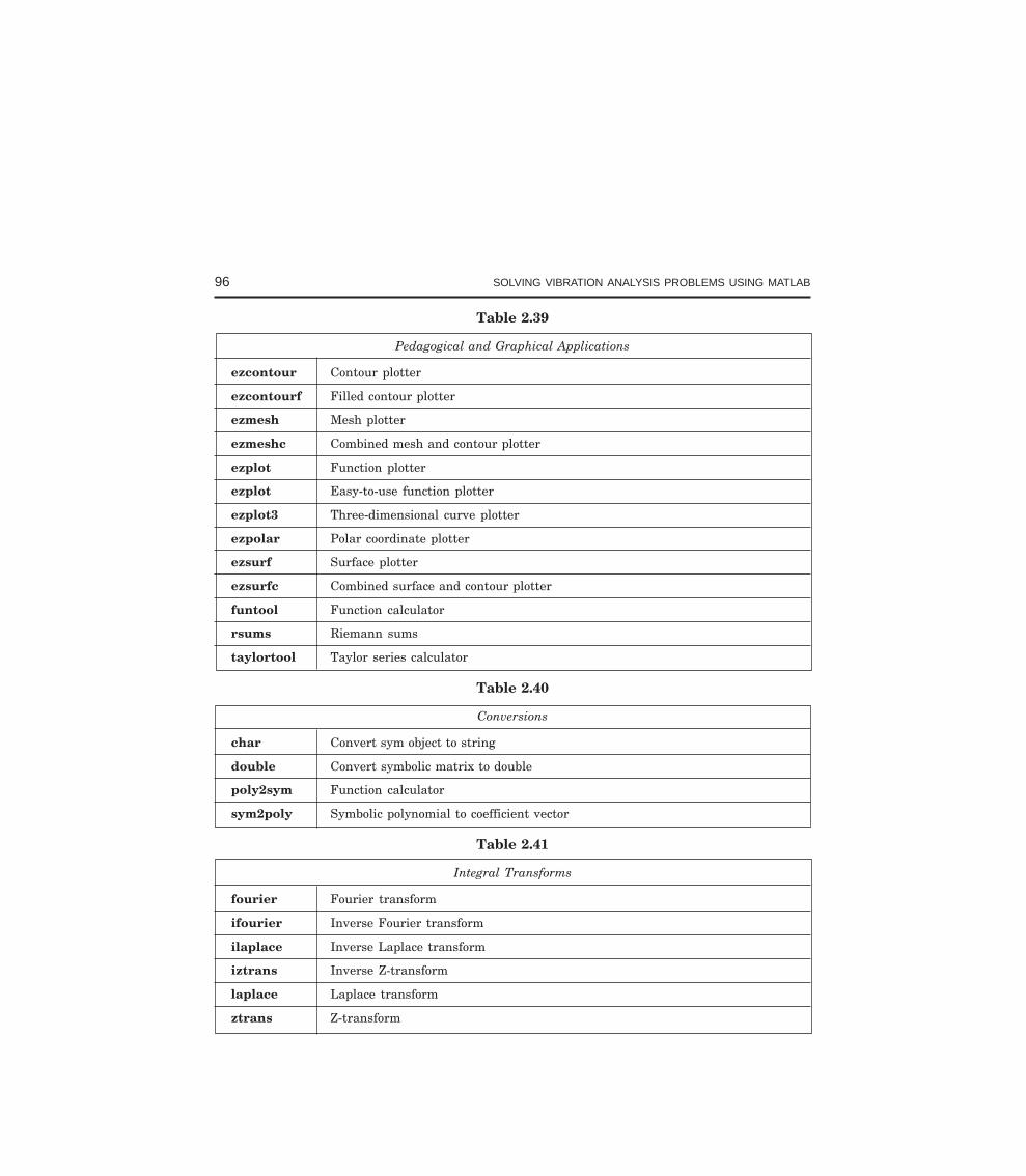
96 SOLVING VIBRATION ANALYSIS PROBLEMS USING MATLAB
Table 2.39
Pedagogical and Graphical Applications
ezcontour Contour plotter
ezcontourf Filled contour plotter
ezmesh Mesh plotter
ezmeshc Combined mesh and contour plotter
ezplot Function plotter
ezplot Easy-to-use function plotter
ezplot3 Three-dimensional curve plotter
ezpolar Polar coordinate plotter
ezsurf Surface plotter
ezsurfc Combined surface and contour plotter
funtool Function calculator
rsums Riemann sums
taylortool Taylor series calculator
Table 2.40
Conversions
char Convert sym object to string
double Convert symbolic matrix to double
poly2sym Function calculator
sym2poly Symbolic polynomial to coefficient vector
Table 2.41
Integral Transforms
fourier Fourier transform
ifourier Inverse Fourier transform
ilaplace Inverse Laplace transform
iztrans Inverse Z-transform
laplace Laplace transform
ztrans Z-transform
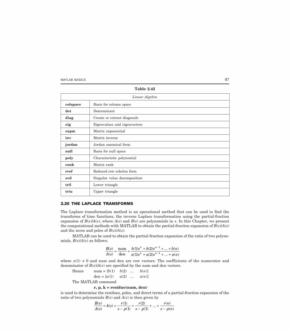
MATLAB BASICS 97
Table 2.42
Linear Algebra
colspace Basis for column space
det Determinant
diag Create or extract diagonals
eig Eigenvalues and eigenvectors
expm Matrix exponential
inv Matrix inverse
jordan Jordan canonical form
null Basis for null space
poly Characteristic polynomial
rank Matrix rank
rref Reduced row echelon form
svd Singular value decomposition
tril Lower triangle
triu Upper triangle
The Laplace transformation method is an operational method that can be used to find thetransforms of time functions, the inverse Laplace transformation using the partial-fractionexpansion of B(s)/A(s), where A(s) and B(s) are polynomials in s. In this Chapter, we presentthe computational methods with MATLAB to obtain the partial-fraction expansion of B(s)/A(s)and the zeros and poles of B(s)/A(s).
MATLAB can be used to obtain the partial-fraction expansion of the ratio of two polyno-mials, B(s)/A(s) as follows:
B sA s
b s b s b na s a s a n
n n
n n( )( )
( ) ( ) ... ( )( ) ( ) ... ( )
= = + + ++ + +
−
−numden
1 21 2
1
1
where a(1) ≠ 0 and num and den are row vectors. The coefficients of the numerator anddenominator of B(s)/A(s) are specified by the num and den vectors.
Hence num = [b(1) b(2) … b(n)]den = [a(1) a(2) … a(n)]
The MATLAB commandr, p, k = residue(num, den)
is used to determine the residues, poles, and direct terms of a partial-fraction expansion of theratio of two polynomials B(s) and A(s) is then given by
B sA s
k sr
s pr
s pr n
s p n( )( )
( )( )
( )( )
( )...
( )( )
= +−
+−
+ +−
11
21
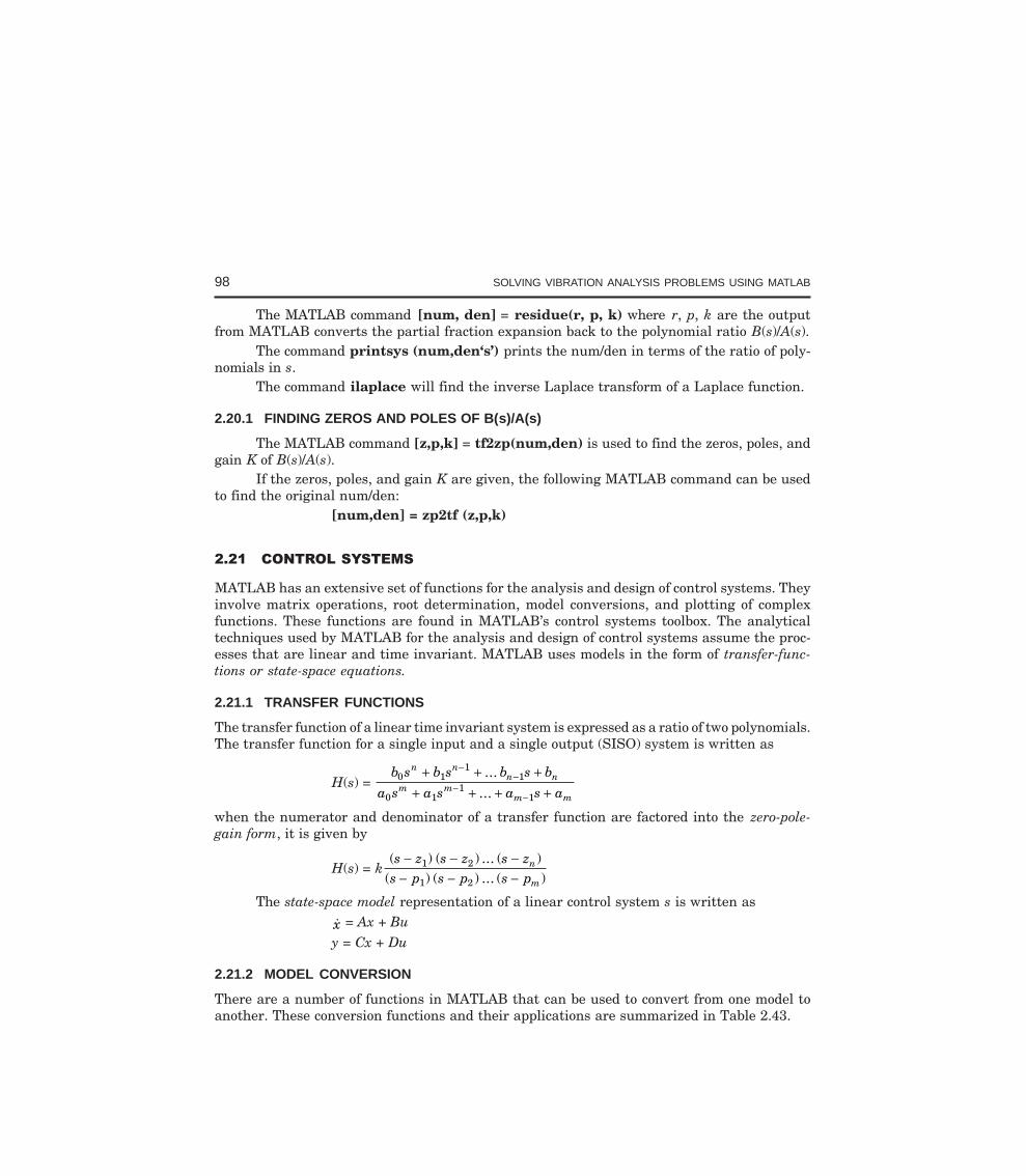
98 SOLVING VIBRATION ANALYSIS PROBLEMS USING MATLAB
The MATLAB command [num, den] = residue(r, p, k) where r, p, k are the outputfrom MATLAB converts the partial fraction expansion back to the polynomial ratio B(s)/A(s).
The command printsys (num,den‘s’) prints the num/den in terms of the ratio of poly-nomials in s.
The command ilaplace will find the inverse Laplace transform of a Laplace function.
2.20.1 FINDING ZEROS AND POLES OF B(s)/A(s)
The MATLAB command [z,p,k] = tf2zp(num,den) is used to find the zeros, poles, andgain K of B(s)/A(s).
If the zeros, poles, and gain K are given, the following MATLAB command can be usedto find the original num/den:
[num,den] = zp2tf (z,p,k)
MATLAB has an extensive set of functions for the analysis and design of control systems. Theyinvolve matrix operations, root determination, model conversions, and plotting of complexfunctions. These functions are found in MATLAB’s control systems toolbox. The analyticaltechniques used by MATLAB for the analysis and design of control systems assume the proc-esses that are linear and time invariant. MATLAB uses models in the form of transfer-func-tions or state-space equations.
2.21.1 TRANSFER FUNCTIONS
The transfer function of a linear time invariant system is expressed as a ratio of two polynomials.The transfer function for a single input and a single output (SISO) system is written as
H(s) = b s b s b s b
a s a s a s a
n nn n
m mm m
0 11
1
0 11
1
+ + ++ + + +
−−
−−
...
...
when the numerator and denominator of a transfer function are factored into the zero-pole-gain form, it is given by
H(s) = k( ) ( ) ... ( )
( ) ( ) ... ( )s z s z s z
s p s p s pn
m
− − −− − −
1 2
1 2
The state-space model representation of a linear control system s is written as
x = Ax + Buy = Cx + Du
2.21.2 MODEL CONVERSION
There are a number of functions in MATLAB that can be used to convert from one model toanother. These conversion functions and their applications are summarized in Table 2.43.
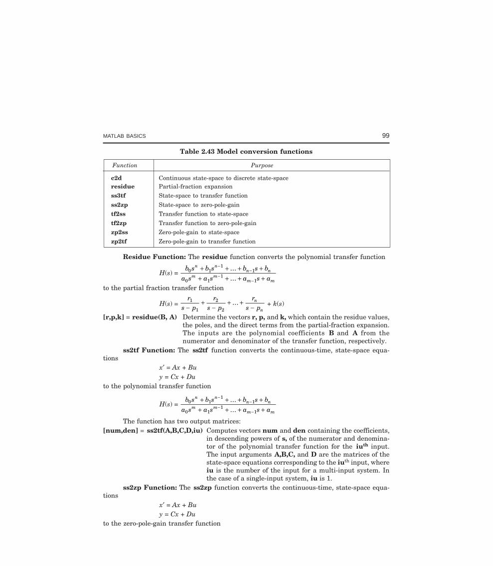
MATLAB BASICS 99
Table 2.43 Model conversion functions
Function Purpose
c2d Continuous state-space to discrete state-spaceresidue Partial-fraction expansion
ss3tf State-space to transfer function
ss2zp State-space to zero-pole-gain
tf2ss Transfer function to state-space
tf2zp Transfer function to zero-pole-gain
zp2ss Zero-pole-gain to state-space
zp2tf Zero-pole-gain to transfer function
Residue Function: The residue function converts the polynomial transfer function
H(s) = b s b s b s b
a s a s a s a
n nn n
m mm m
0 11
1
0 11
1
+ + + ++ + + +
−−
−−
...
...to the partial fraction transfer function
H(s) = r
s pr
s pr
s pn
n
1
1
2
2−+
−+ +
−... + k(s)
[r,p,k] = residue(B, A) Determine the vectors r, p, and k, which contain the residue values,the poles, and the direct terms from the partial-fraction expansion.The inputs are the polynomial coefficients B and A from thenumerator and denominator of the transfer function, respectively.
ss2tf Function: The ss2tf function converts the continuous-time, state-space equa-tions
x′ = Ax + Buy = Cx + Du
to the polynomial transfer function
H(s) = b s b s b s b
a s a s a s a
n nn n
m mm m
0 11
1
0 11
1
+ + + ++ + + +
−−
−−
...
...
The function has two output matrices:[num,den] = ss2tf(A,B,C,D,iu) Computes vectors num and den containing the coefficients,
in descending powers of s, of the numerator and denomina-tor of the polynomial transfer function for the iuth input.The input arguments A,B,C, and D are the matrices of thestate-space equations corresponding to the iuth input, whereiu is the number of the input for a multi-input system. Inthe case of a single-input system, iu is 1.
ss2zp Function: The ss2zp function converts the continuous-time, state-space equa-tions
x′ = Ax + Buy = Cx + Du
to the zero-pole-gain transfer function
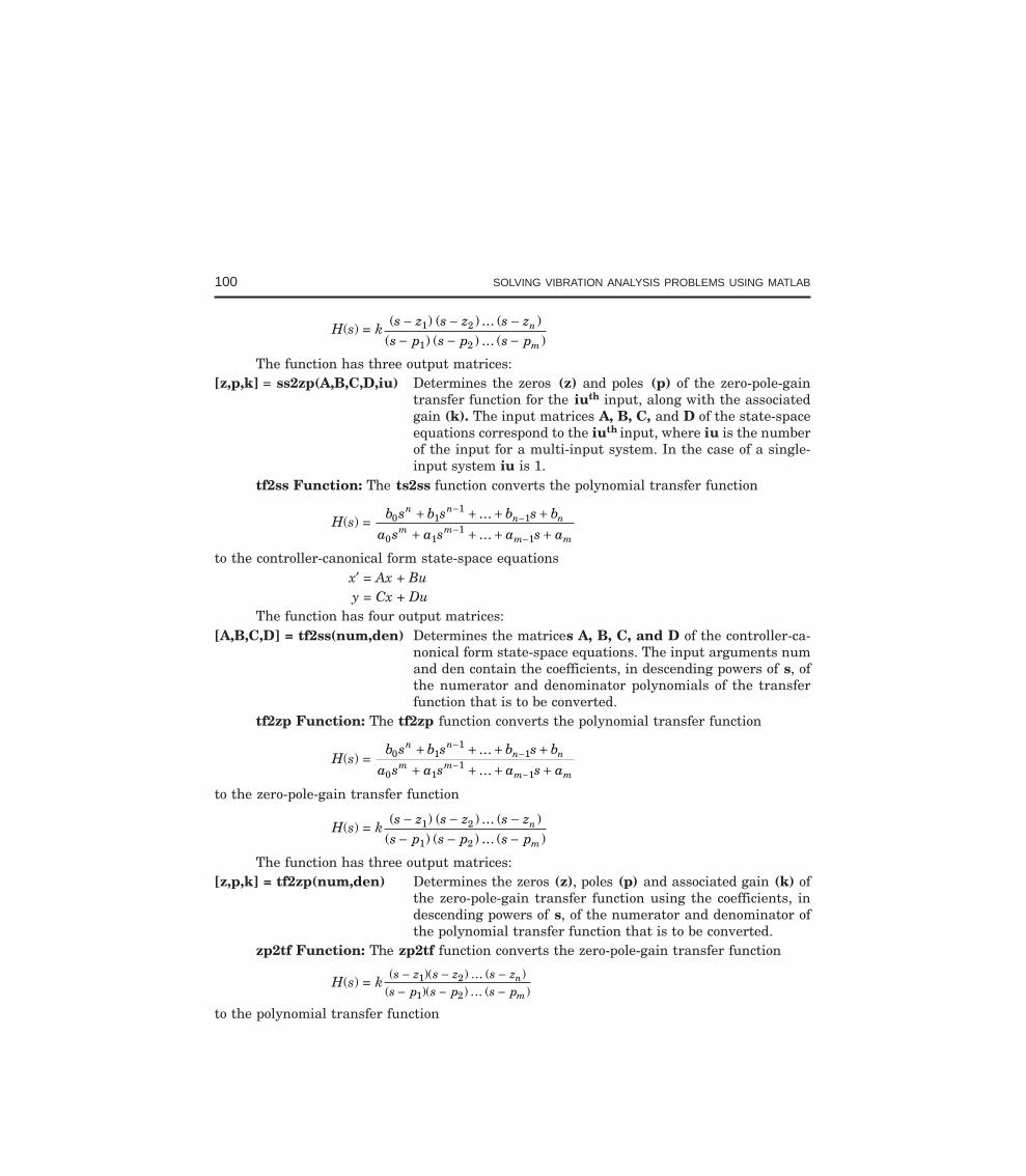
100 SOLVING VIBRATION ANALYSIS PROBLEMS USING MATLAB
H(s) = k ( ) ( ) ... ( )( ) ( ) ... ( )
s z s z s zs p s p s p
n
m
− − −− − −
1 2
1 2
The function has three output matrices:[z,p,k] = ss2zp(A,B,C,D,iu) Determines the zeros (z) and poles (p) of the zero-pole-gain
transfer function for the iuth input, along with the associatedgain (k). The input matrices A, B, C, and D of the state-spaceequations correspond to the iuth input, where iu is the numberof the input for a multi-input system. In the case of a single-input system iu is 1.
tf2ss Function: The ts2ss function converts the polynomial transfer function
H(s) = b s b s b s b
a s a s a s a
n nn n
m mm m
0 11
1
0 11
1
+ + + ++ + + +
−−
−−
...
...
to the controller-canonical form state-space equationsx′ = Ax + Buy = Cx + Du
The function has four output matrices:[A,B,C,D] = tf2ss(num,den) Determines the matrices A, B, C, and D of the controller-ca-
nonical form state-space equations. The input arguments numand den contain the coefficients, in descending powers of s, ofthe numerator and denominator polynomials of the transferfunction that is to be converted.
tf2zp Function: The tf2zp function converts the polynomial transfer function
H(s) = b s b s b s b
a s a s a s a
n nn n
m mm m
0 11
1
0 11
1
+ + + ++ + + +
−−
−−
...
...
to the zero-pole-gain transfer function
H(s) = k( ) ( ) ... ( )
( ) ( ) ... ( )s z s z s z
s p s p s pn
m
− − −− − −
1 2
1 2
The function has three output matrices:[z,p,k] = tf2zp(num,den) Determines the zeros (z), poles (p) and associated gain (k) of
the zero-pole-gain transfer function using the coefficients, indescending powers of s, of the numerator and denominator ofthe polynomial transfer function that is to be converted.
zp2tf Function: The zp2tf function converts the zero-pole-gain transfer function
H(s) = k( )( ) ... ( )
( )( ) ... ( )s z s z s z
s p s p s pn
m
− − −− − −
1 2
1 2
to the polynomial transfer function
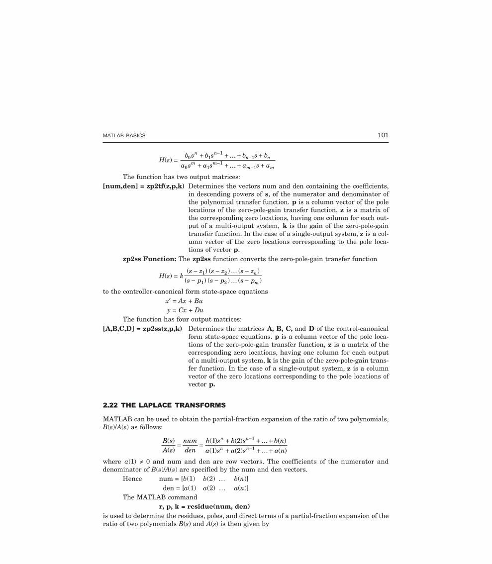
MATLAB BASICS 101
H(s) = b s b s b s b
a s a s a s a
n nn n
m mm m
0 11
1
0 11
1
+ + + ++ + + +
−−
−−
...
...
The function has two output matrices:[num,den] = zp2tf(z,p,k) Determines the vectors num and den containing the coefficients,
in descending powers of s, of the numerator and denominator ofthe polynomial transfer function. p is a column vector of the polelocations of the zero-pole-gain transfer function, z is a matrix ofthe corresponding zero locations, having one column for each out-put of a multi-output system, k is the gain of the zero-pole-gaintransfer function. In the case of a single-output system, z is a col-umn vector of the zero locations corresponding to the pole loca-tions of vector p.
zp2ss Function: The zp2ss function converts the zero-pole-gain transfer function
H(s) = k( ) ( ) ... ( )
( ) ( ) ... ( )s z s z s z
s p s p s pn
m
− − −− − −
1 2
1 2
to the controller-canonical form state-space equationsx′ = Ax + Buy = Cx + Du
The function has four output matrices:[A,B,C,D] = zp2ss(z,p,k) Determines the matrices A, B, C, and D of the control-canonical
form state-space equations. p is a column vector of the pole loca-tions of the zero-pole-gain transfer function, z is a matrix of thecorresponding zero locations, having one column for each outputof a multi-output system, k is the gain of the zero-pole-gain trans-fer function. In the case of a single-output system, z is a columnvector of the zero locations corresponding to the pole locations ofvector p.
MATLAB can be used to obtain the partial-fraction expansion of the ratio of two polynomials,B(s)/A(s) as follows:
B sA s
numden
b s b s b na s a s a n
n n
n n( )( )
( ) ( ) ... ( )( ) ( ) ... ( )
= = + + ++ + +
−
−1 21 2
1
1
where a(1) ≠ 0 and num and den are row vectors. The coefficients of the numerator anddenominator of B(s)/A(s) are specified by the num and den vectors.
Hence num = [b(1) b(2) … b(n)] den = [a(1) a(2) … a(n)]
The MATLAB commandr, p, k = residue(num, den)
is used to determine the residues, poles, and direct terms of a partial-fraction expansion of theratio of two polynomials B(s) and A(s) is then given by
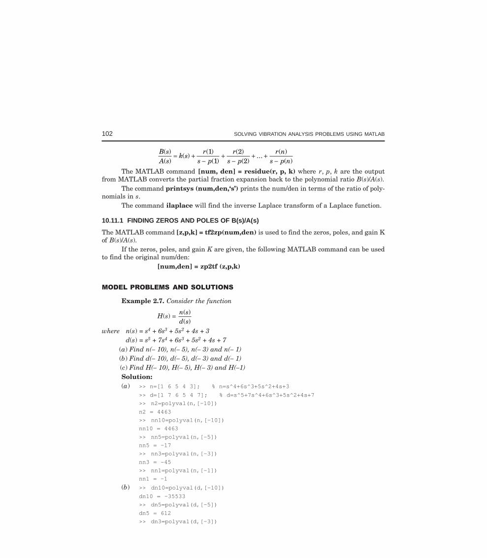
102 SOLVING VIBRATION ANALYSIS PROBLEMS USING MATLAB
B sA s
k sr
s pr
s pr n
s p n( )( )
( )( )
( )( )
( )...
( )( )
= +−
+−
+ +−
11
22
The MATLAB command [num, den] = residue(r, p, k) where r, p, k are the outputfrom MATLAB converts the partial fraction expansion back to the polynomial ratio B(s)/A(s).
The command printsys (num,den,‘s’) prints the num/den in terms of the ratio of poly-nomials in s.
The command ilaplace will find the inverse Laplace transform of a Laplace function.
10.11.1 FINDING ZEROS AND POLES OF B(s)/A(s)
The MATLAB command [z,p,k] = tf2zp(num,den) is used to find the zeros, poles, and gain Kof B(s)/A(s).
If the zeros, poles, and gain K are given, the following MATLAB command can be usedto find the original num/den:
[num,den] = zp2tf (z,p,k)
Example 2.7. Consider the function
H(s) = n sd s
( )( )
where n(s) = s4 + 6s3 + 5s2 + 4s + 3d(s) = s5 + 7s4 + 6s3 + 5s2 + 4s + 7
(a) Find n(– 10), n(– 5), n(– 3) and n(– 1)(b) Find d(– 10), d(– 5), d(– 3) and d(– 1)(c) Find H(– 10), H(– 5), H(– 3) and H(–1)Solution:(a) >> n=[1 6 5 4 3]; % n=s^4+6s^3+5s^2+4s+3
>> d=[1 7 6 5 4 7]; % d=s^5+7s^4+6s^3+5s^2+4s+7
>> n2=polyval(n,[-10])
n2 = 4463
>> nn10=polyval(n,[-10])
nn10 = 4463
>> nn5=polyval(n,[-5])
nn5 = -17
>> nn3=polyval(n,[-3])
nn3 = -45
>> nn1=polyval(n,[-1])
nn1 = -1
(b) >> dn10=polyval(d,[-10])
dn10 = -35533
>> dn5=polyval(d,[-5])
dn5 = 612
>> dn3=polyval(d,[-3])
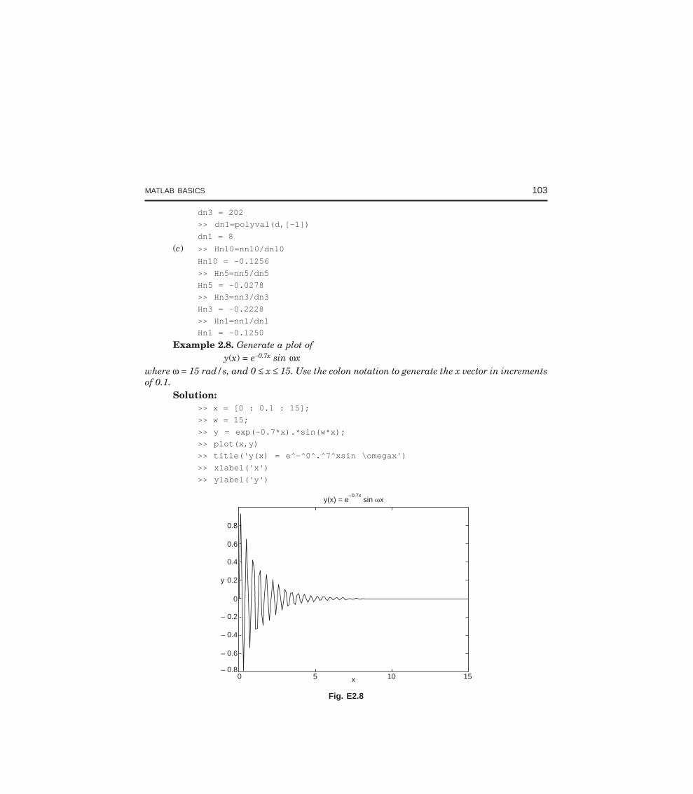
MATLAB BASICS 103
dn3 = 202
>> dn1=polyval(d,[-1])
dn1 = 8
(c) >> Hn10=nn10/dn10
Hn10 = -0.1256
>> Hn5=nn5/dn5
Hn5 = -0.0278
>> Hn3=nn3/dn3
Hn3 = -0.2228
>> Hn1=nn1/dn1
Hn1 = -0.1250
Example 2.8. Generate a plot ofy(x) = e–0.7x sin ωx
where ω = 15 rad/s, and 0 ≤ x ≤ 15. Use the colon notation to generate the x vector in incrementsof 0.1.
Solution:>> x = [0 : 0.1 : 15];
>> w = 15;
>> y = exp(-0.7*x).*sin(w*x);
>> plot(x,y)
>> title('y(x) = e^-^0^.^7^xsin \omegax')
>> xlabel('x')
>> ylabel('y')
0.8
0.6
0.4
0.2
0
– 0.2
– 0.4
– 0.6
– 0.80 5 10 15x
y(x) = e sin x–0.7x
y
Fig. E2.8
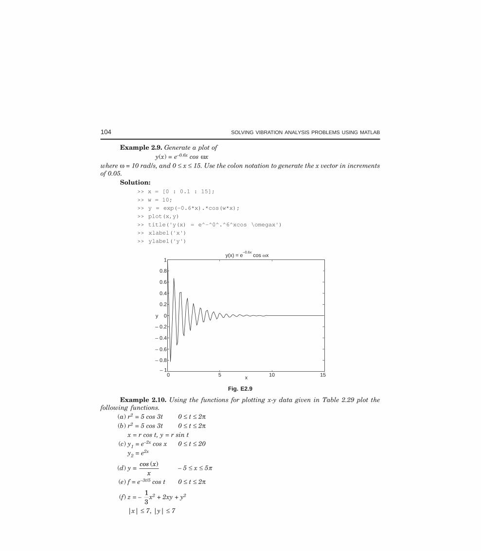
104 SOLVING VIBRATION ANALYSIS PROBLEMS USING MATLAB
Example 2.9. Generate a plot ofy(x) = e–0.6x cos ωx
where ω = 10 rad/s, and 0 ≤ x ≤ 15. Use the colon notation to generate the x vector in incrementsof 0.05.
Solution:>> x = [0 : 0.1 : 15];
>> w = 10;
>> y = exp(-0.6*x).*cos(w*x);
>> plot(x,y)
>> title('y(x) = e^-^0^.^6^xcos \omegax')
>> xlabel('x')
>> ylabel('y')
y(x) = e cos x–0.6x
0 5 10 15– 1
– 0.8
– 0.6
– 0.4
– 0.2
0
0.2
0.4
0.6
0.8
1
y
x
Fig. E2.9
Example 2.10. Using the functions for plotting x-y data given in Table 2.29 plot thefollowing functions.
(a) r2 = 5 cos 3t 0 ≤ t ≤ 2π(b) r2 = 5 cos 3t 0 ≤ t ≤ 2π
x = r cos t, y = r sin t(c) y1 = e–2x cos x 0 ≤ t ≤ 20
y2 = e2x
(d) y = cos x
x( )
– 5 ≤ x ≤ 5π
(e) f = e–3t/5 cos t 0 ≤ t ≤ 2π
(f) z = – 13
x2 + 2xy + y2
|x| ≤ 7, |y| ≤ 7
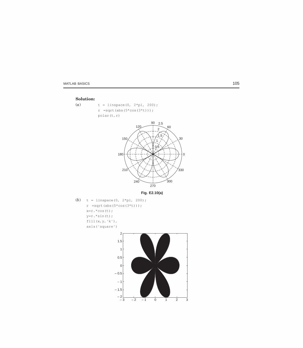
MATLAB BASICS 105
Solution:(a) t = linspace(0, 2*pi, 200);
r =sqrt(abs(5*cos(3*t)));
polar(t,r)
150
180
210
240270
300
330
0
30
6090
1202.5
2
1.5
1
0.5
Fig. E2.10(a)
(b) t = linspace(0, 2*pi, 200);
r =sqrt(abs(5*cos(3*t)));
x=r.*cos(t);
y=r.*sin(t);
fill(x,y,'k'),
axis('square')
– 3 – 2 – 1 0 21 3– 2
– 1.5
– 1
– 0.5
0
0.5
1
1.5
2
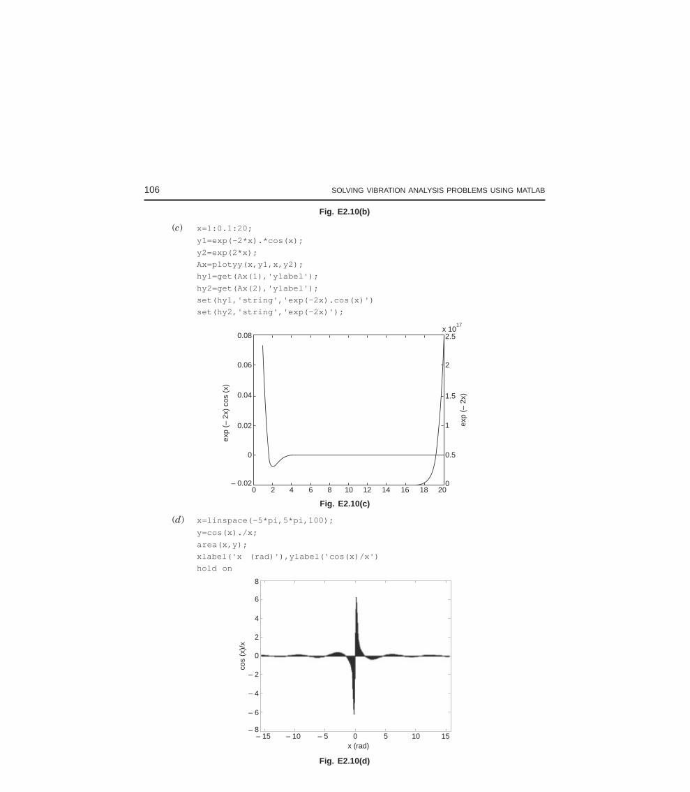
106 SOLVING VIBRATION ANALYSIS PROBLEMS USING MATLAB
Fig. E2.10(b)
(c) x=1:0.1:20;
y1=exp(-2*x).*cos(x);
y2=exp(2*x);
Ax=plotyy(x,y1,x,y2);
hy1=get(Ax(1),'ylabel');
hy2=get(Ax(2),'ylabel');
set(hy1,'string','exp(-2x).cos(x)')
set(hy2,'string','exp(-2x)');
0.08
0.06
0.04
0.02
0
– 0.02
2.5x 10
17
2
1.5
1
0.5
0
exp
(–2x
)
0 2 4 6 8 10 12 14 16 18 20
exp
(–2x
)co
s(x
)
Fig. E2.10(c)
(d) x=linspace(-5*pi,5*pi,100);
y=cos(x)./x;
area(x,y);
xlabel('x (rad)'),ylabel('cos(x)/x')
hold on
x (rad)– 15 – 10 – 5 0 5 10 15
– 8
– 6
– 4
– 2
0
2
4
6
8
cos
(x)/
x
Fig. E2.10(d)
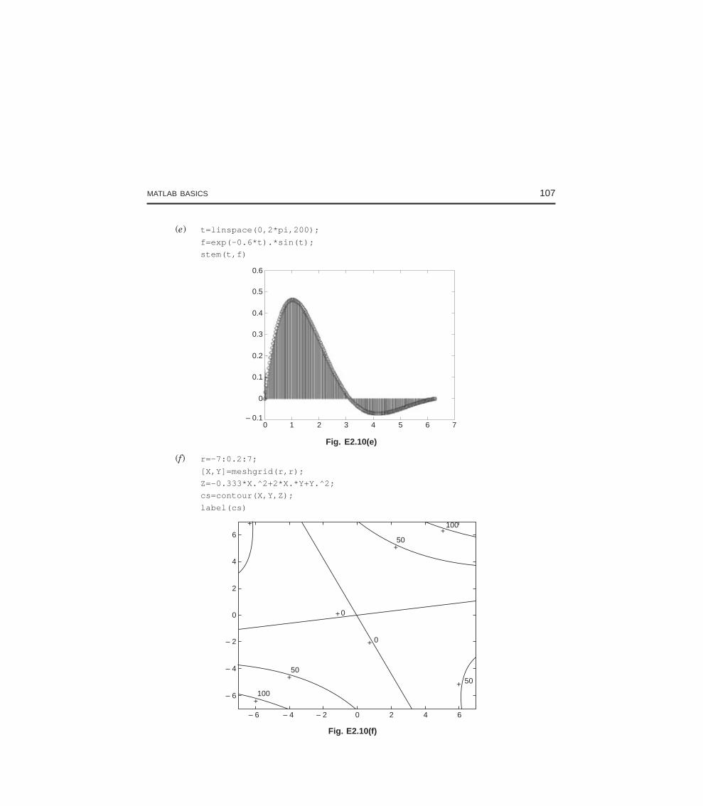
MATLAB BASICS 107
(e) t=linspace(0,2*pi,200);
f=exp(-0.6*t).*sin(t);
stem(t,f)
0.6
0.5
0.4
0.3
0.2
0.1
0
– 0.10 1 2 3 4 5 6 7
Fig. E2.10(e)
(f) r=-7:0.2:7;
[X,Y]=meshgrid(r,r);
Z=-0.333*X.^2+2*X.*Y+Y.^2;
cs=contour(X,Y,Z);
label(cs)
+
+
+
+
+
+
+50
100
0
0
5050
100
+
– 6 – 4 – 2 0 2 4 6
– 6
– 4
– 2
0
2
4
6
Fig. E2.10(f)
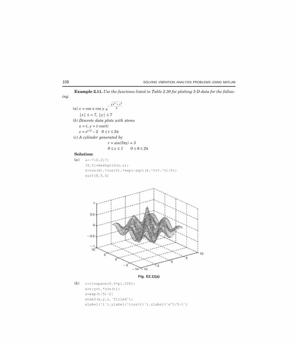
108 SOLVING VIBRATION ANALYSIS PROBLEMS USING MATLAB
Example 2.11. Use the functions listed in Table 2.30 for plotting 3-D data for the follow-ing.
(a) z = cos x cos y ex y
5
2 2
−+
|x| ≤ = 7, |y| ≤ 7(b) Discrete data plots with stems
x = t, y = t cos(t)z = et/5 – 2 0 ≤ t ≤ 5π
(c) A cylinder generated byr = sin(5πz) + 30 ≤ z ≤ 1 0 ≤ θ ≤ 2π
Solution:(a) u=-7:0.2:7;
[X,Y]=meshgrid(u,u);
Z=cos(X).*cos(Y).*exp(-sqrt(X.^2+Y.^2)/5);
surf(X,Y,Z)
Fig. E2.11(a)
(b) t=linspace(0,5*pi,200);
x=t;y=t.*cos(t);
z=exp(t/5)-2;
stem3(x,y,z,'filled');
xlabel('t'),ylabel('tcos(t)'),zlabel('e^t/5-1')
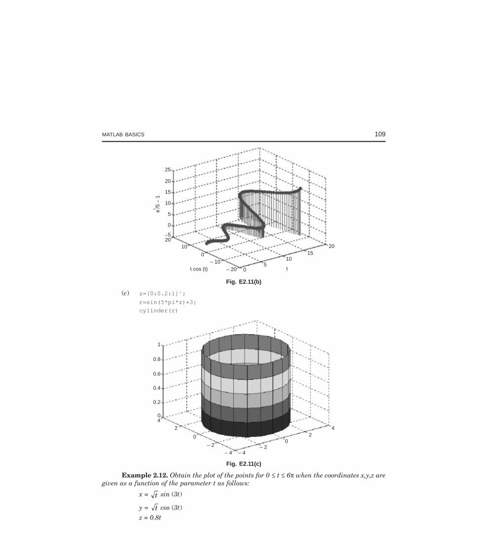
MATLAB BASICS 109
25
20
15
10
5
0
–520
10
0– 10
– 20 05
1015
20
tt cos (t)
e/5
–1
t
Fig. E2.11(b)
(c) z=[0:0.2:1]';
r=sin(5*pi*z)+3;
cylinder(r)
1
0.8
0.6
0.4
0.2
04
2
0
– 2
– 4 – 4– 2
02
4
Fig. E2.11(c)
Example 2.12. Obtain the plot of the points for 0 ≤ t ≤ 6π when the coordinates x,y,z aregiven as a function of the parameter t as follows:
x = t sin (3t)
y = t cos (3t)z = 0.8t
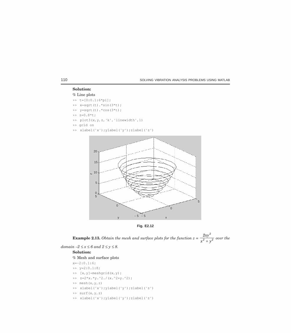
110 SOLVING VIBRATION ANALYSIS PROBLEMS USING MATLAB
Solution:% Line plots>> t=[0:0.1:6*pi];
>> x=sqrt(t).*sin(3*t);
>> y=sqrt(t).*cos(3*t);
>> z=0.8*t;
>> plot3(x,y,z,'k','linewidth',1)
>> grid on
>> xlabel('x');ylabel('y');zlabel('z')
– 5– 5– 5– 5
00
5500
55
00
xxyy
55
1010
1515
2020
zz
Fig. E2.12
Example 2.13. Obtain the mesh and surface plots for the function z = 2xy
x y
2
2 2+ over the
domain –2 ≤ x ≤ 6 and 2 ≤ y ≤ 8.Solution:% Mesh and surface plotsx=-2:0.1:6;
>> y=2:0.1:8;
>> [x,y]=meshgrid(x,y);
>> z=2*x.*y.^2./(x.^2+y.^2);
>> mesh(x,y,z)
>> xlabel('x');ylabel('y');zlabel('z')
>> surf(x,y,z)
>> xlabel('x');ylabel('y');zlabel('z')
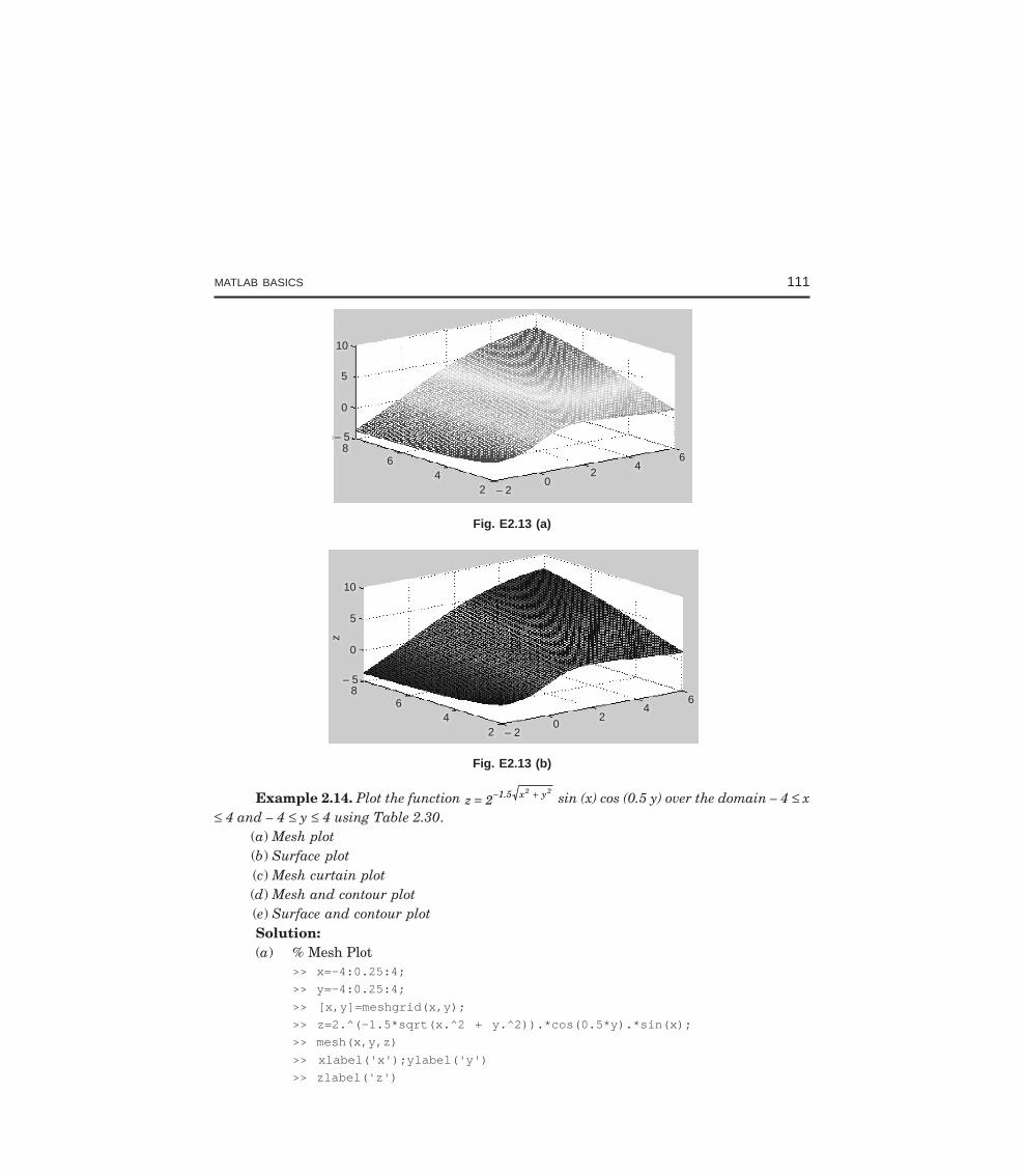
MATLAB BASICS 111
88
00
– 5– 5
55
1010
6644
22 – 2– 200
2244
66
Fig. E2.13 (a)
88
00
– 5– 5
55
1010
6644
22 – 2– 200
2244
66
zz
Fig. E2.13 (b)
Example 2.14. Plot the function z 2 1.5 x y2 2
= − + sin (x) cos (0.5 y) over the domain – 4 ≤ x≤ 4 and – 4 ≤ y ≤ 4 using Table 2.30.
(a) Mesh plot(b) Surface plot(c) Mesh curtain plot(d) Mesh and contour plot(e) Surface and contour plotSolution:(a) % Mesh Plot
>> x=-4:0.25:4;
>> y=-4:0.25:4;
>> [x,y]=meshgrid(x,y);
>> z=2.^(-1.5*sqrt(x.^2 + y.^2)).*cos(0.5*y).*sin(x);
>> mesh(x,y,z)
>> xlabel('x');ylabel('y')
>> zlabel('z')
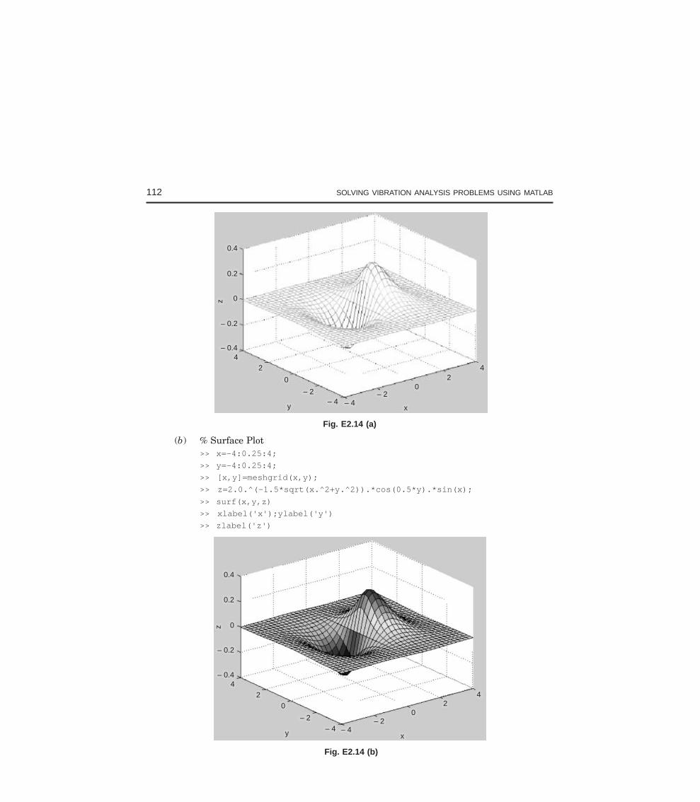
112 SOLVING VIBRATION ANALYSIS PROBLEMS USING MATLAB
– 0.4– 0.4
– 0.2– 0.2
00
0.20.2
0.40.4
44
zz
22
00
– 2– 2– 4– 4 – 4– 4
– 2– 200
2244
yy xx
Fig. E2.14 (a)
(b) % Surface Plot>> x=-4:0.25:4;
>> y=-4:0.25:4;
>> [x,y]=meshgrid(x,y);
>> z=2.0.^(-1.5*sqrt(x.^2+y.^2)).*cos(0.5*y).*sin(x);
>> surf(x,y,z)
>> xlabel('x');ylabel('y')
>> zlabel('z')
0.40.4
0.20.2
00
– 0.2– 0.2
– 0.4– 0.444
2200
– 2– 2– 4– 4 – 4– 4
– 2– 200
2244
xxyy
zz
Fig. E2.14 (b)
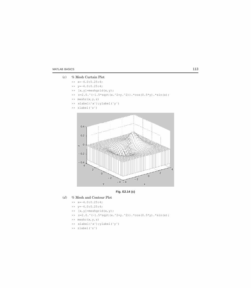
MATLAB BASICS 113
(c) % Mesh Curtain Plot>> x=-4.0:0.25:4;
>> y=-4.0:0.25:4;
>> [x,y]=meshgrid(x,y);
>> z=2.0.^(-1.5*sqrt(x.^2+y.^2)).*cos(0.5*y).*sin(x);
>> meshz(x,y,z)
>> xlabel('x');ylabel('y')
>> zlabel('z')
0.40.4
0.20.2
00
– 0.2– 0.2
– 0.4– 0.444
22
00
– 2– 2
– 4– 4 – 4– 4– 2– 2
0022
44
yy xx
zz
Fig. E2.14 (c)
(d) % Mesh and Contour Plot>> x=-4.0:0.25:4;
>> y=-4.0:0.25:4;
>> [x,y]=meshgrid(x,y);
>> z=2.0.^(-1.5*sqrt(x.^2+y.^2)).*cos(0.5*y).*sin(x);
>> meshc(x,y,z)
>> xlabel('x');ylabel('y')
>> zlabel('z')
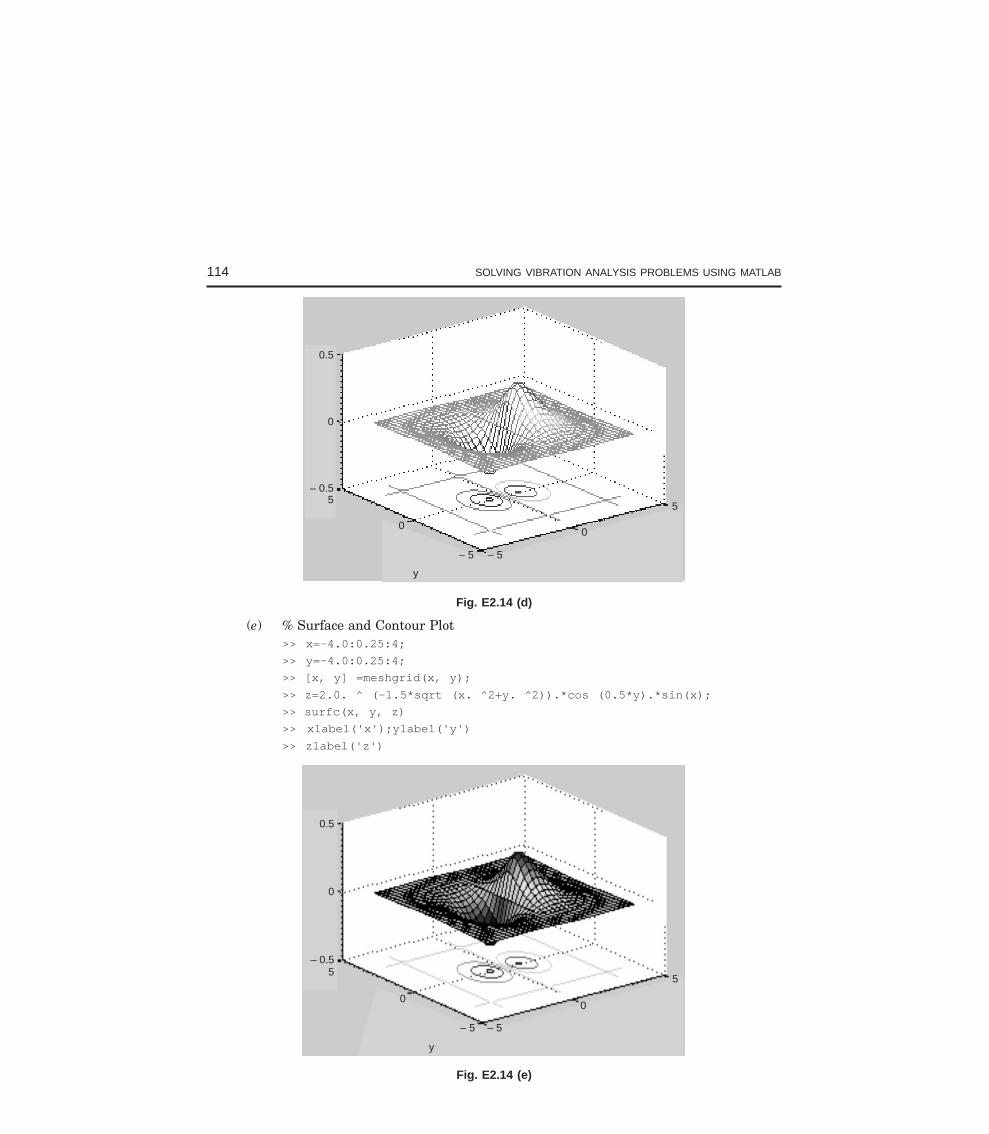
114 SOLVING VIBRATION ANALYSIS PROBLEMS USING MATLAB
0.5
0
– 0.55
0
– 5 – 5
0
5
y
Fig. E2.14 (d)
(e) % Surface and Contour Plot>> x=-4.0:0.25:4;
>> y=-4.0:0.25:4;
>> [x, y] =meshgrid(x, y);
>> z=2.0. ^ (-1.5*sqrt (x. ^2+y. ^2)).*cos (0.5*y).*sin(x);
>> surfc(x, y, z)
>> xlabel('x');ylabel('y')
>> zlabel('z')
0.5
0
– 0.55
0
– 5 – 5
0
5
y
Fig. E2.14 (e)
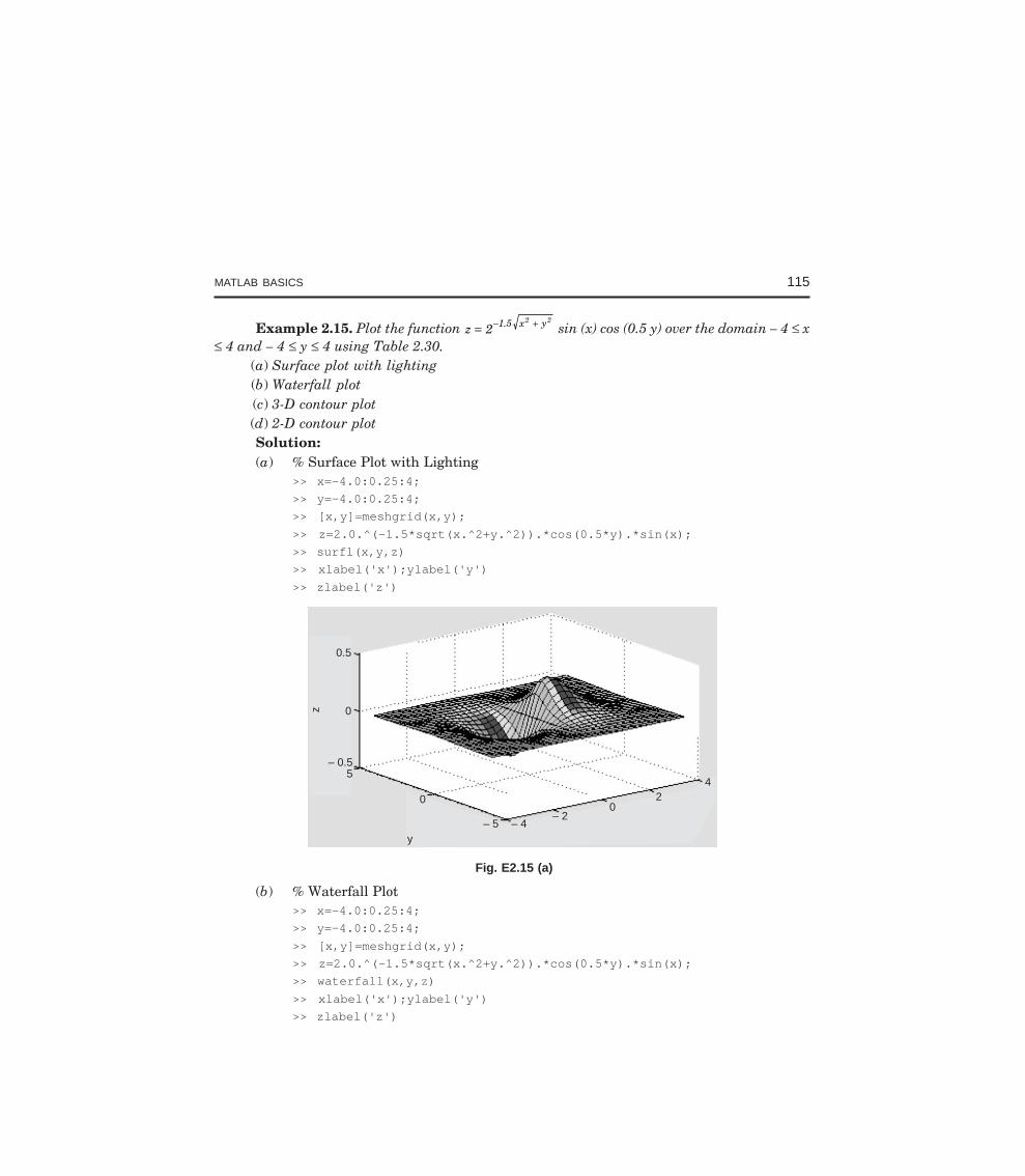
MATLAB BASICS 115
Example 2.15. Plot the function z 2 1.5 x y2 2
= − + sin (x) cos (0.5 y) over the domain – 4 ≤ x≤ 4 and – 4 ≤ y ≤ 4 using Table 2.30.
(a) Surface plot with lighting(b) Waterfall plot(c) 3-D contour plot(d) 2-D contour plotSolution:(a) % Surface Plot with Lighting
>> x=-4.0:0.25:4;
>> y=-4.0:0.25:4;
>> [x,y]=meshgrid(x,y);
>> z=2.0.^(-1.5*sqrt(x.^2+y.^2)).*cos(0.5*y).*sin(x);
>> surfl(x,y,z)
>> xlabel('x');ylabel('y')
>> zlabel('z')
0.5
0
– 0.55
0
– 5 – 4– 2
02
4
y
z
Fig. E2.15 (a)
(b) % Waterfall Plot>> x=-4.0:0.25:4;
>> y=-4.0:0.25:4;
>> [x,y]=meshgrid(x,y);
>> z=2.0.^(-1.5*sqrt(x.^2+y.^2)).*cos(0.5*y).*sin(x);
>> waterfall(x,y,z)
>> xlabel('x');ylabel('y')
>> zlabel('z')
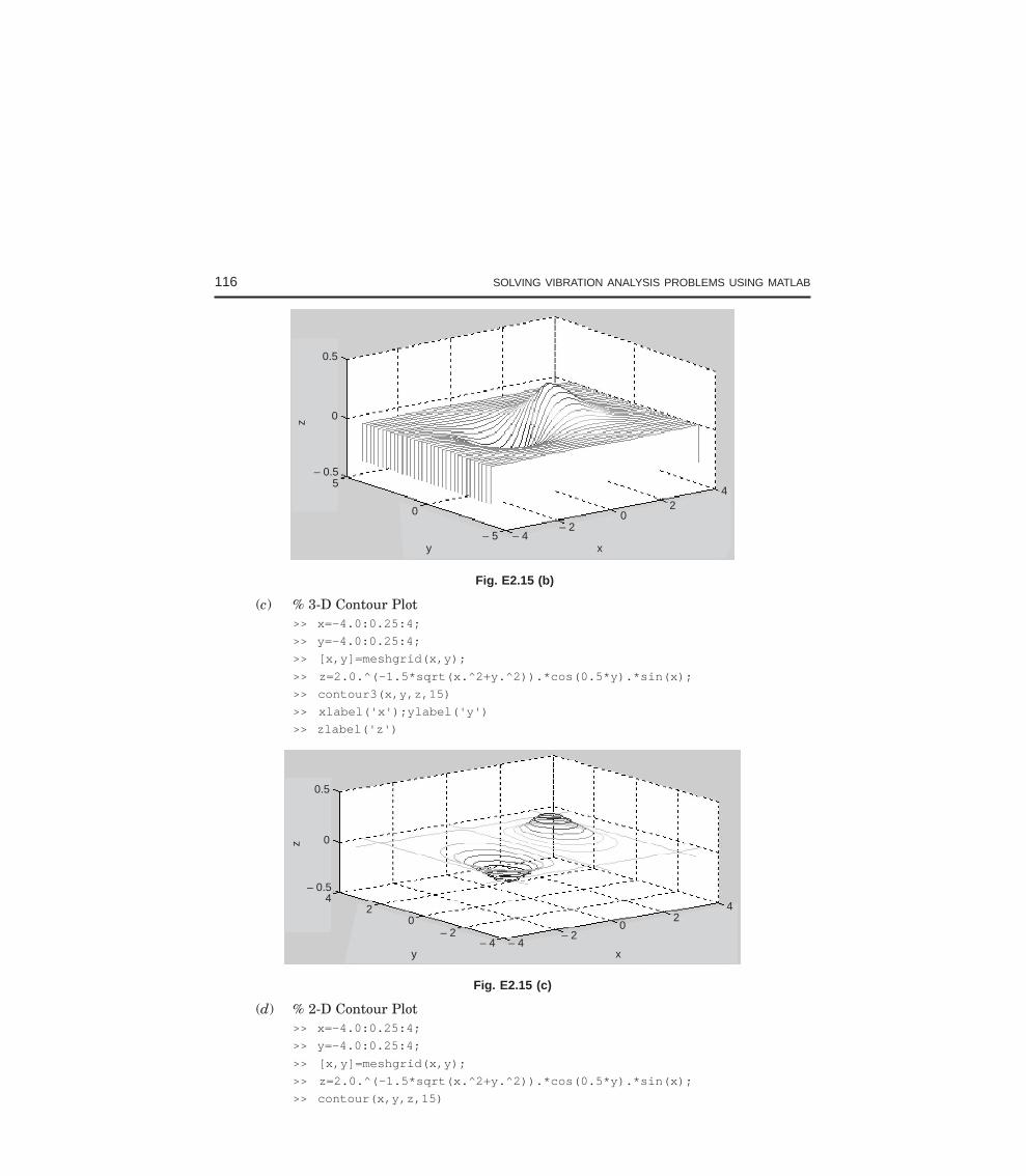
116 SOLVING VIBRATION ANALYSIS PROBLEMS USING MATLAB
0.5
0
– 0.55
z
0
– 5 – 4– 2
02
4
y x
Fig. E2.15 (b)
(c) % 3-D Contour Plot>> x=-4.0:0.25:4;
>> y=-4.0:0.25:4;
>> [x,y]=meshgrid(x,y);
>> z=2.0.^(-1.5*sqrt(x.^2+y.^2)).*cos(0.5*y).*sin(x);
>> contour3(x,y,z,15)
>> xlabel('x');ylabel('y')
>> zlabel('z')
0.5
0
– 0.54
z
20
– 2– 4 – 4
– 20
24
y x
Fig. E2.15 (c)
(d) % 2-D Contour Plot>> x=-4.0:0.25:4;
>> y=-4.0:0.25:4;
>> [x,y]=meshgrid(x,y);
>> z=2.0.^(-1.5*sqrt(x.^2+y.^2)).*cos(0.5*y).*sin(x);
>> contour(x,y,z,15)
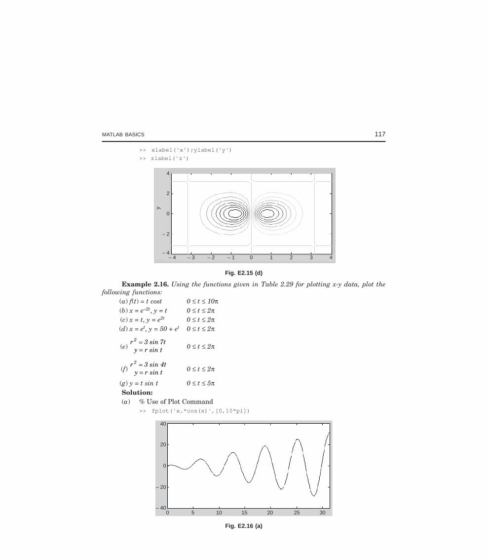
MATLAB BASICS 117
>> xlabel('x');ylabel('y')
>> zlabel('z')
4
2
0
– 2
– 4– 4 – 3 – 2 – 1 0 1 2 3 4
y
Fig. E2.15 (d)
Example 2.16. Using the functions given in Table 2.29 for plotting x-y data, plot thefollowing functions:
(a) f(t) = t cost 0 ≤ t ≤ 10π(b) x = e–2t, y = t 0 ≤ t ≤ 2π(c) x = t, y = e2t 0 ≤ t ≤ 2π(d) x = et, y = 50 + et 0 ≤ t ≤ 2π
(e)r 3 sin 7t
y r sin t
2 == 0 ≤ t ≤ 2π
(f)r 3 sin 4t
y r sin t
2 == 0 ≤ t ≤ 2π
(g) y = t sin t 0 ≤ t ≤ 5πSolution:(a) % Use of Plot Command
>> fplot('x.*cos(x)',[0,10*pi])
40
20
0
– 20
– 400 5 10 15 20 25 30
Fig. E2.16 (a)
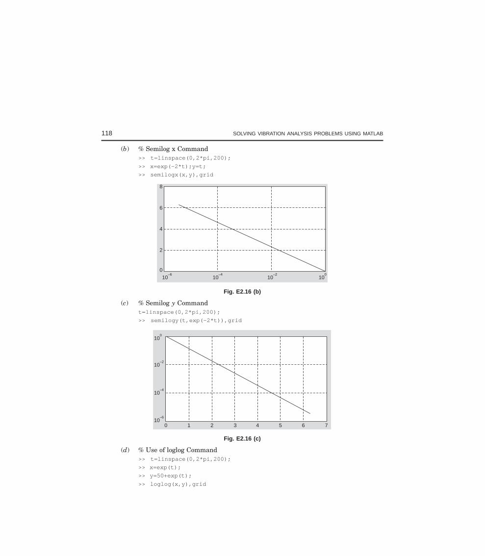
118 SOLVING VIBRATION ANALYSIS PROBLEMS USING MATLAB
(b) % Semilog x Command>> t=linspace(0,2*pi,200);
>> x=exp(-2*t);y=t;
>> semilogx(x,y),grid
8
6
4
2
010
–610
–410
–210
0
Fig. E2.16 (b)
(c) % Semilog y Commandt=linspace(0,2*pi,200);
>> semilogy(t,exp(-2*t)),grid
10–6
10–4
10–2
100
0 1 2 3 4 5 6 7
Fig. E2.16 (c)
(d) % Use of loglog Command>> t=linspace(0,2*pi,200);
>> x=exp(t);
>> y=50+exp(t);
>> loglog(x,y),grid
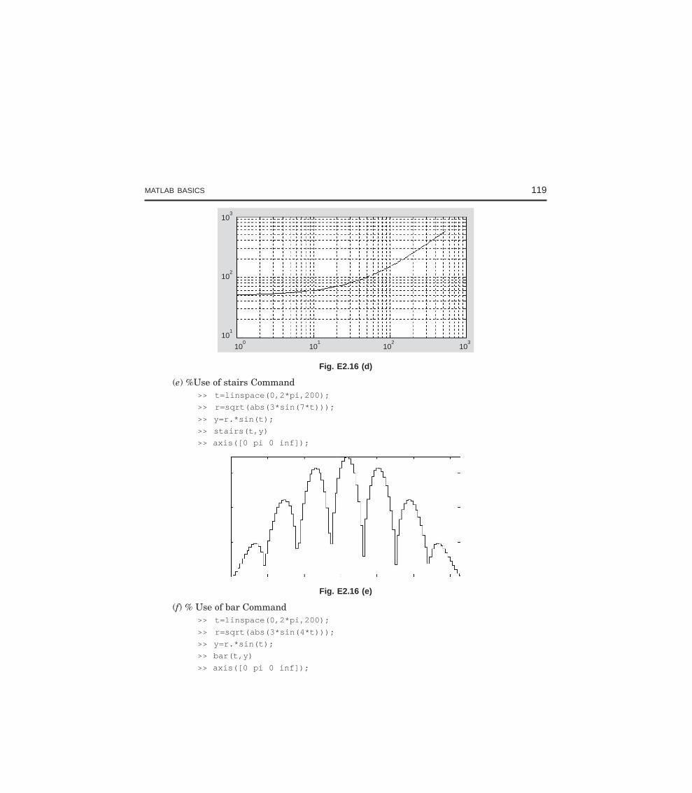
MATLAB BASICS 119
103
102
101
100
101
102
103
Fig. E2.16 (d)
(e) %Use of stairs Command>> t=linspace(0,2*pi,200);
>> r=sqrt(abs(3*sin(7*t)));
>> y=r.*sin(t);
>> stairs(t,y)
>> axis([0 pi 0 inf]);
Fig. E2.16 (e)
(f) % Use of bar Command>> t=linspace(0,2*pi,200);
>> r=sqrt(abs(3*sin(4*t)));
>> y=r.*sin(t);
>> bar(t,y)
>> axis([0 pi 0 inf]);
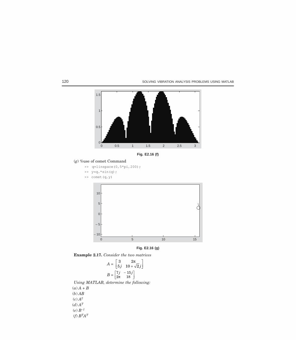
120 SOLVING VIBRATION ANALYSIS PROBLEMS USING MATLAB
1.5
1
0.5
00 0.5 1 1.5 2 2.5 3
Fig. E2.16 (f)
(g) %use of comet Command>> q=linspace(0,5*pi,200);
>> y=q.*sin(q);
>> comet(q,y)
10
5
0
– 5
– 10
0 5 10 15
Fig. E2.16 (g)
Example 2.17. Consider the two matrices
A = 3 25 10 2
πj j+
LNM
OQP
B = 7 152 18
j j−LNM
OQPπ
Using MATLAB, determine the following:(a) A + B(b) AB(c) A2
(d) AT
(e) B–1
(f) BTAT
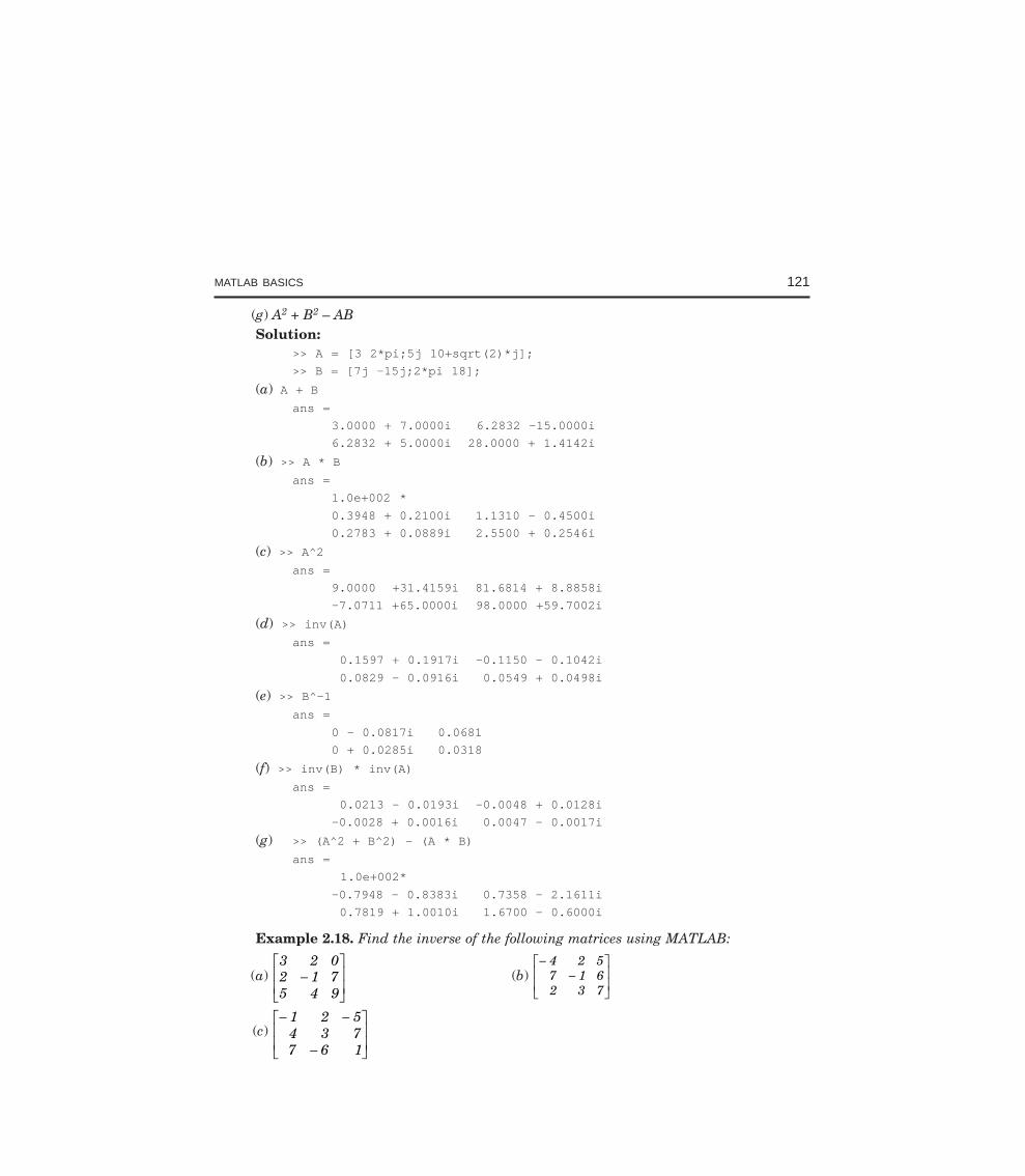
MATLAB BASICS 121
(g) A2 + B2 – ABSolution:
>> A = [3 2*pi;5j 10+sqrt(2)*j];
>> B = [7j -15j;2*pi 18];
(a) A + Bans =
3.0000 + 7.0000i 6.2832 -15.0000i
6.2832 + 5.0000i 28.0000 + 1.4142i
(b) >> A * Bans =
1.0e+002 *
0.3948 + 0.2100i 1.1310 - 0.4500i
0.2783 + 0.0889i 2.5500 + 0.2546i
(c) >> A^2ans =
9.0000 +31.4159i 81.6814 + 8.8858i
-7.0711 +65.0000i 98.0000 +59.7002i
(d) >> inv(A)ans =
0.1597 + 0.1917i -0.1150 - 0.1042i
0.0829 - 0.0916i 0.0549 + 0.0498i
(e) >> B^-1ans =
0 - 0.0817i 0.0681
0 + 0.0285i 0.0318
(f) >> inv(B) * inv(A)ans =
0.0213 - 0.0193i -0.0048 + 0.0128i
-0.0028 + 0.0016i 0.0047 - 0.0017i
(g) >> (A^2 + B^2) - (A * B)
ans =
1.0e+002*
-0.7948 - 0.8383i 0.7358 - 2.1611i
0.7819 + 1.0010i 1.6700 - 0.6000i
Example 2.18. Find the inverse of the following matrices using MATLAB:
(a)3 2 02 1 75 4 9
−L
NMM
O
QPP (b)
−−
L
NMM
O
QPP
4 2 57 1 62 3 7
(c)− −
−
L
NMM
O
QPP
1 2 54 3 77 6 1
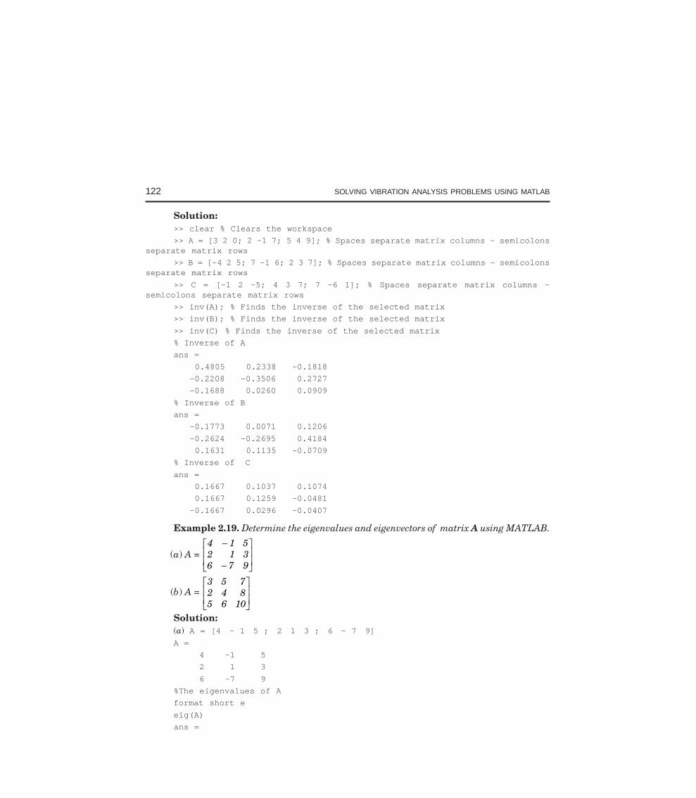
122 SOLVING VIBRATION ANALYSIS PROBLEMS USING MATLAB
Solution:>> clear % Clears the workspace
>> A = [3 2 0; 2 -1 7; 5 4 9]; % Spaces separate matrix columns - semicolonsseparate matrix rows
>> B = [-4 2 5; 7 -1 6; 2 3 7]; % Spaces separate matrix columns - semicolonsseparate matrix rows
>> C = [-1 2 -5; 4 3 7; 7 -6 1]; % Spaces separate matrix columns -semicolons separate matrix rows
>> inv(A); % Finds the inverse of the selected matrix
>> inv(B); % Finds the inverse of the selected matrix
>> inv(C) % Finds the inverse of the selected matrix
% Inverse of A
ans =
0.4805 0.2338 -0.1818
-0.2208 -0.3506 0.2727
-0.1688 0.0260 0.0909
% Inverse of B
ans =
-0.1773 0.0071 0.1206
-0.2624 -0.2695 0.4184
0.1631 0.1135 -0.0709
% Inverse of C
ans =
0.1667 0.1037 0.1074
0.1667 0.1259 -0.0481
-0.1667 0.0296 -0.0407
Example 2.19. Determine the eigenvalues and eigenvectors of matrix A using MATLAB.
(a) A = 4 1 52 1 36 7 9
−
−
L
NMM
O
QPP
(b) A = 3 5 72 4 85 6 10
L
NMM
O
QPP
Solution:(a) A = [4 – 1 5 ; 2 1 3 ; 6 – 7 9]
A =
4 -1 5
2 1 3
6 -7 9
%The eigenvalues of A
format short e
eig(A)
ans =
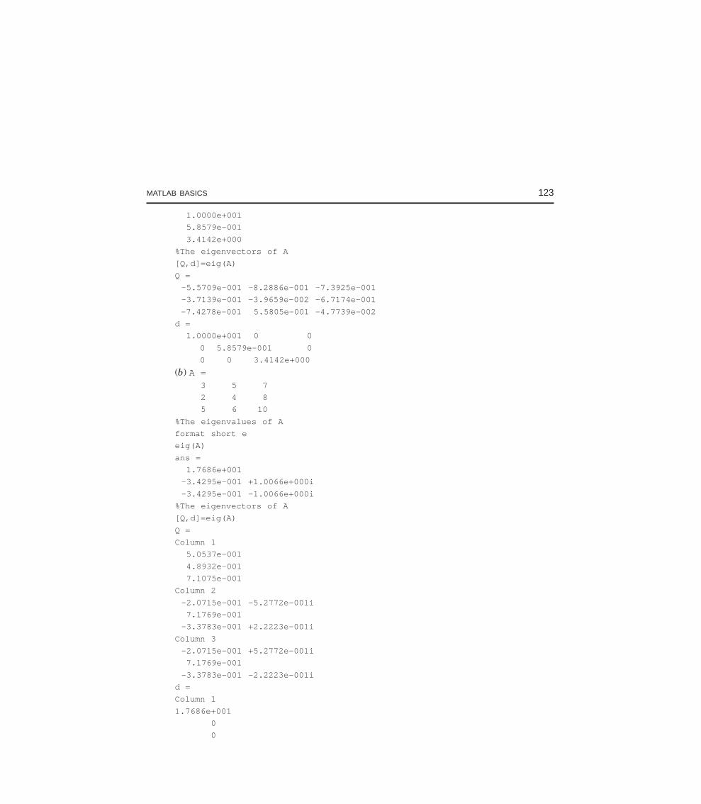
MATLAB BASICS 123
1.0000e+001
5.8579e-001
3.4142e+000
%The eigenvectors of A
[Q,d]=eig(A)
Q =
-5.5709e-001 -8.2886e-001 -7.3925e-001
-3.7139e-001 -3.9659e-002 -6.7174e-001
-7.4278e-001 5.5805e-001 -4.7739e-002
d =
1.0000e+001 0 0
0 5.8579e-001 0
0 0 3.4142e+000
(b) A = 3 5 7
2 4 8
5 6 10
%The eigenvalues of A
format short e
eig(A)
ans =
1.7686e+001
-3.4295e-001 +1.0066e+000i
-3.4295e-001 -1.0066e+000i
%The eigenvectors of A
[Q,d]=eig(A)
Q =
Column 1
5.0537e-001
4.8932e-001
7.1075e-001
Column 2
-2.0715e-001 -5.2772e-001i
7.1769e-001
-3.3783e-001 +2.2223e-001i
Column 3
-2.0715e-001 +5.2772e-001i
7.1769e-001
-3.3783e-001 -2.2223e-001i
d =
Column 1
1.7686e+001
0
0
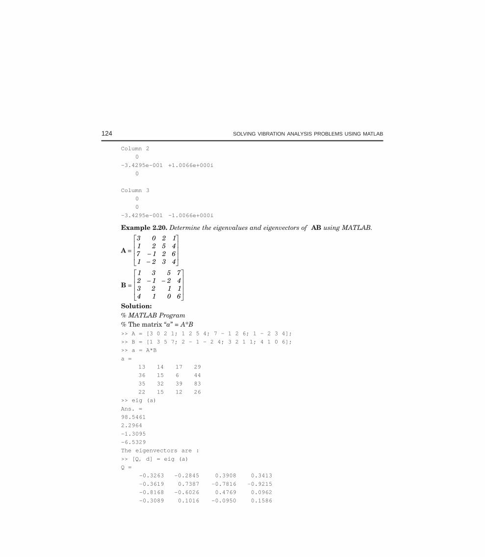
124 SOLVING VIBRATION ANALYSIS PROBLEMS USING MATLAB
Column 2
0
-3.4295e-001 +1.0066e+000i
0
Column 3
0
0
-3.4295e-001 -1.0066e+000i
Example 2.20. Determine the eigenvalues and eigenvectors of AB using MATLAB.
A =
3 0 2 11 2 5 47 1 2 61 2 3 4
−−
L
N
MMM
O
Q
PPP
B =
1 3 5 72 1 2 43 2 1 14 1 0 6
− −L
N
MMM
O
Q
PPP
Solution:% MATLAB Program% The matrix “a” = A*B>> A = [3 0 2 1; 1 2 5 4; 7 – 1 2 6; 1 – 2 3 4];
>> B = [1 3 5 7; 2 – 1 – 2 4; 3 2 1 1; 4 1 0 6];
>> a = A*B
a =
13 14 17 29
36 15 6 44
35 32 39 83
22 15 12 26
>> eig (a)
Ans. =
98.5461
2.2964
–1.3095
–6.5329
The eigenvectors are :
>> [Q, d] = eig (a)
Q =
–0.3263 –0.2845 0.3908 0.3413
–0.3619 0.7387 –0.7816 –0.9215
–0.8168 –0.6026 0.4769 0.0962
–0.3089 0.1016 –0.0950 0.1586
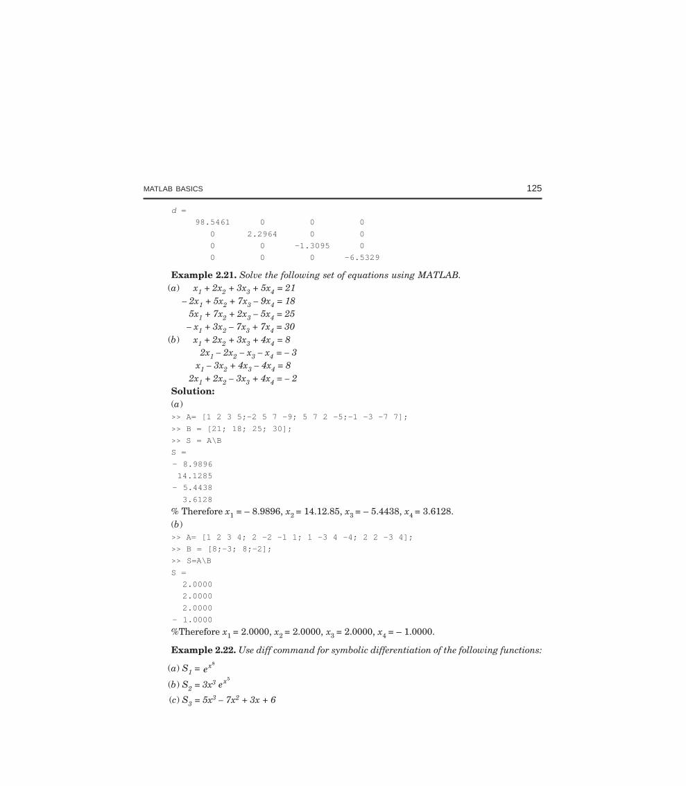
MATLAB BASICS 125
d =
98.5461 0 0 0
0 2.2964 0 0
0 0 –1.3095 0
0 0 0 –6.5329
Example 2.21. Solve the following set of equations using MATLAB.(a) x1 + 2x2 + 3x3 + 5x4 = 21
– 2x1 + 5x2 + 7x3 – 9x4 = 185x1 + 7x2 + 2x3 – 5x4 = 25– x1 + 3x2 – 7x3 + 7x4 = 30
(b) x1 + 2x2 + 3x3 + 4x4 = 82x1 – 2x2 – x3 – x4 = – 3
x1 – 3x2 + 4x3 – 4x4 = 82x1 + 2x2 – 3x3 + 4x4 = – 2
Solution:(a)>> A= [1 2 3 5;–2 5 7 –9; 5 7 2 –5;–1 –3 –7 7];
>> B = [21; 18; 25; 30];
>> S = A\B
S =
– 8.9896
14.1285
– 5.4438
3.6128
% Therefore x1 = – 8.9896, x2 = 14.12.85, x3 = – 5.4438, x4 = 3.6128.(b)>> A= [1 2 3 4; 2 -2 -1 1; 1 -3 4 -4; 2 2 -3 4];
>> B = [8;-3; 8;-2];
>> S=A\B
S =
2.0000
2.0000
2.0000
– 1.0000
%Therefore x1 = 2.0000, x2 = 2.0000, x3 = 2.0000, x4 = – 1.0000.
Example 2.22. Use diff command for symbolic differentiation of the following functions:
(a) S1 = ex8
(b) S2 = 3x3 ex5
(c) S3 = 5x3 – 7x2 + 3x + 6
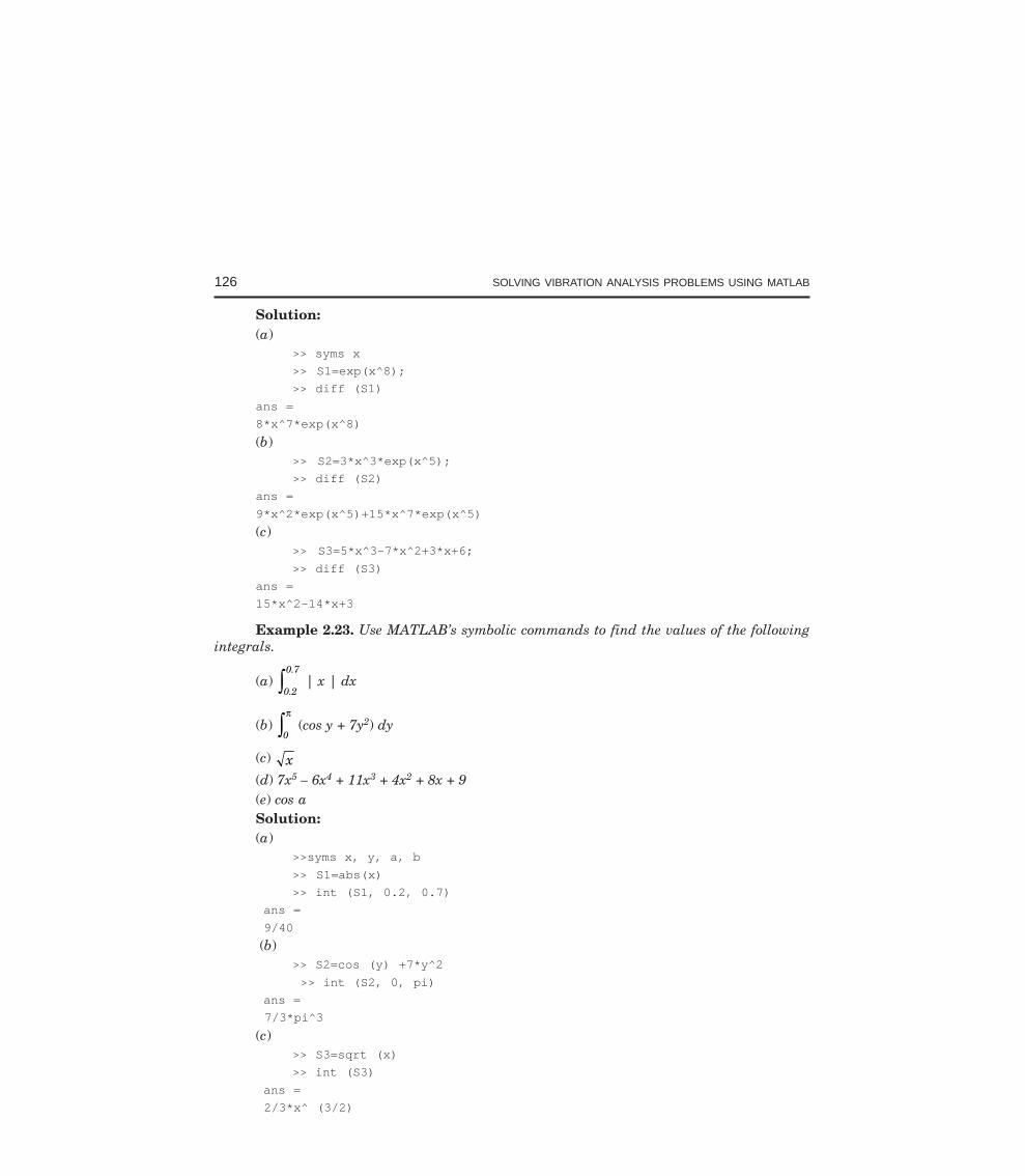
126 SOLVING VIBRATION ANALYSIS PROBLEMS USING MATLAB
Solution:(a)
>> syms x
>> S1=exp(x^8);
>> diff (S1)
ans =
8*x^7*exp(x^8)
(b)>> S2=3*x^3*exp(x^5);
>> diff (S2)
ans =
9*x^2*exp(x^5)+15*x^7*exp(x^5)
(c)>> S3=5*x^3-7*x^2+3*x+6;
>> diff (S3)
ans =
15*x^2-14*x+3
Example 2.23. Use MATLAB’s symbolic commands to find the values of the followingintegrals.
(a) 0.2
0.7z | x | dx
(b) 0
πz (cos y + 7y2) dy
(c) x(d) 7x5 – 6x4 + 11x3 + 4x2 + 8x + 9(e) cos aSolution:(a)
>>syms x, y, a, b
>> S1=abs(x)
>> int (S1, 0.2, 0.7)
ans =
9/40
(b)>> S2=cos (y) +7*y^2
>> int (S2, 0, pi)
ans =
7/3*pi^3
(c)>> S3=sqrt (x)
>> int (S3)
ans =
2/3*x^ (3/2)
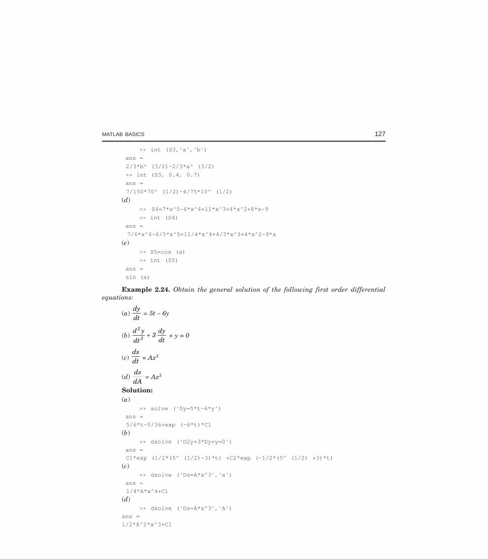
MATLAB BASICS 127
>> int (S3,'a','b')
ans =
2/3*b^ (3/2)-2/3*a^ (3/2)
>> int (S3, 0.4, 0.7)
ans =
7/150*70^ (1/2)-4/75*10^ (1/2)
(d)>> S4=7*x^5-6*x^4+11*x^3+4*x^2+8*x-9
>> int (S4)
ans =
7/6*x^6-6/5*x^5+11/4*x^4+4/3*x^3+4*x^2-9*x
(e)>> S5=cos (a)
>> int (S5)
ans =
sin (a)
Example 2.24. Obtain the general solution of the following first order differentialequations:
(a) dydt
= 5t – 6y
(b) d y
dt3
dydt
2
2 + + y = 0
(c) dsdt = Ax3
(d) dsdA
= Ax3
Solution:(a)
>> solve ('Dy=5*t-6*y')
ans =
5/6*t-5/36+exp (-6*t)*C1
(b)>> dsolve ('D2y+3*Dy+y=0')
ans =
C1*exp (1/2*(5^ (1/2)-3)*t) +C2*exp (-1/2*(5^ (1/2) +3)*t)
(c)>> dsolve ('Ds=A*x^3','x')
ans =
1/4*A*x^4+C1
(d)>> dsolve ('Ds=A*x^3','A')
ans =
1/2*A^2*x^3+C1
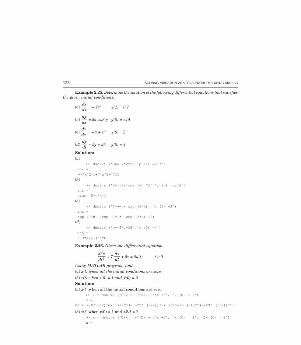
128 SOLVING VIBRATION ANALYSIS PROBLEMS USING MATLAB
Example 2.25. Determine the solution of the following differential equations that satisfiesthe given initial conditions.
(a) dydx
= – 7x2 y(1) = 0.7
(b) dydx
= 5x cos2 y y(0) = π/4
(c) dydx
= – y + e3x y(0) = 2
(d) dydt
+ 5y = 35 y(0) = 4
Solution:(a)
>> dsolve ('Dy=-7*x^2','y (1) =0.7')
ans =
-7*x^2*t+7*x^2+7/10
(b)>> dsolve ('Dy=5*x*cos (y) ^2','y (0) =pi/4')
ans =
atan (5*t*x+1)
(c)>> dsolve ('Dy=-y+ exp (3*x)','y (0) =2')
ans =
exp (3*x) +exp (-t)*(-exp (3*x) +2)
(d)>> dsolve ('Dy+5*y=35','y (0) =4')
ans =
7-3*exp (-5*t)
Example 2.26. Given the differential equation
d x
dt
2
2 + 7 dxdt
+ 5x = 8u(t) t ≥ 0
Using MATLAB program, find(a) x(t) when all the initial conditions are zero
(b) x(t) when x(0) = 1 and x(0) = 2.Solution:(a) x(t) when all the initial conditions are zero
>> x = dsolve ('D2x = -7*Dx - 5*x +8', 'x (0) = 0')
x =
8/5+ (-8/5-C2)*exp (1/2*(-7+29^ (1/2))*t) +C2*exp (-1/2*(7+29^ (1/2))*t)
(b) x(t) when x(0) = 1 and x(0) = 2>> x = dsolve ('D2x = -7*Dx - 5*x +8', 'x (0) = 1', 'Dx (0) = 2')
x =
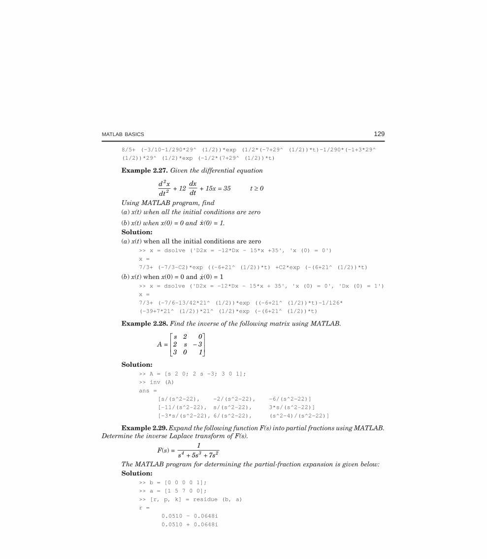
MATLAB BASICS 129
8/5+ (-3/10-1/290*29^ (1/2))*exp (1/2*(-7+29^ (1/2))*t)-1/290*(-1+3*29^
(1/2))*29^ (1/2)*exp (-1/2*(7+29^ (1/2))*t)
Example 2.27. Given the differential equation
d x
dt
2
2 + 12 dxdt
+ 15x = 35 t ≥ 0
Using MATLAB program, find(a) x(t) when all the initial conditions are zero
(b) x(t) when x(0) = 0 and x(0) = 1.Solution:(a) x(t) when all the initial conditions are zero
>> x = dsolve ('D2x = -12*Dx - 15*x +35', 'x (0) = 0')
x =
7/3+ (-7/3-C2)*exp ((-6+21^ (1/2))*t) +C2*exp (-(6+21^ (1/2))*t)
(b) x(t) when x(0) = 0 and x(0) = 1>> x = dsolve ('D2x = -12*Dx - 15*x + 35', 'x (0) = 0', 'Dx (0) = 1')
x =
7/3+ (-7/6-13/42*21^ (1/2))*exp ((-6+21^ (1/2))*t)-1/126*
(-39+7*21^ (1/2))*21^ (1/2)*exp (-(6+21^ (1/2))*t)
Example 2.28. Find the inverse of the following matrix using MATLAB.
A = s 2 02 s 33 0 1
−L
NMM
O
QPP
Solution:>> A = [s 2 0; 2 s -3; 3 0 1];
>> inv (A)
ans =
[s/(s^2-22), -2/(s^2-22), -6/(s^2-22)]
[-11/(s^2-22), s/(s^2-22), 3*s/(s^2-22)]
[-3*s/(s^2-22), 6/(s^2-22), (s^2-4)/(s^2-22)]
Example 2.29. Expand the following function F(s) into partial fractions using MATLAB.Determine the inverse Laplace transform of F(s).
F(s) = 1
s 5s 7s4 3 2+ +The MATLAB program for determining the partial-fraction expansion is given below:Solution:
>> b = [0 0 0 0 1];
>> a = [1 5 7 0 0];
>> [r, p, k] = residue (b, a)
r =
0.0510 - 0.0648i
0.0510 + 0.0648i
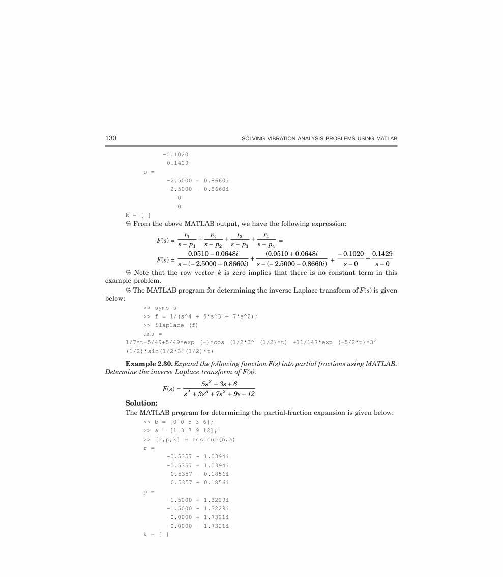
130 SOLVING VIBRATION ANALYSIS PROBLEMS USING MATLAB
-0.1020
0.1429
p =
-2.5000 + 0.8660i
-2.5000 - 0.8660i
0
0
k = [ ]
% From the above MATLAB output, we have the following expression:
F(s) = r
s pr
s pr
s pr
s p1
1
2
2
3
3
4
4−+
−+
−+
− =
F(s) = 0 0510 0 0648
2 5000 0 86600 0510 0 0648
2 5000 0 8660. .
( . . )( . .( . . )
−− − +
+ +− − −
is i
is i +
−−
+−
0 10200
0 14290
. .s s
% Note that the row vector k is zero implies that there is no constant term in thisexample problem.
% The MATLAB program for determining the inverse Laplace transform of F(s) is givenbelow:
>> syms s
>> f = 1/(s^4 + 5*s^3 + 7*s^2);
>> ilaplace (f)
ans =
1/7*t-5/49+5/49*exp (-)*cos (1/2*3^ (1/2)*t) +11/147*exp (-5/2*t)*3^
(1/2)*sin(1/2*3^(1/2)*t)
Example 2.30. Expand the following function F(s) into partial fractions using MATLAB.Determine the inverse Laplace transform of F(s).
F(s) = 5s 3s 6
s 3s 7s 9s 12
2
4 3 2+ +
+ + + +Solution:The MATLAB program for determining the partial-fraction expansion is given below:
>> b = [0 0 5 3 6];
>> a = [1 3 7 9 12];
>> [r,p,k] = residue(b,a)
r =
-0.5357 - 1.0394i
-0.5357 + 1.0394i
0.5357 - 0.1856i
0.5357 + 0.1856i
p =
-1.5000 + 1.3229i
-1.5000 - 1.3229i
-0.0000 + 1.7321i
-0.0000 - 1.7321i
k = [ ]
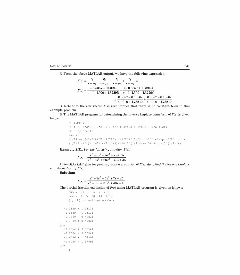
MATLAB BASICS 131
% From the above MATLAB output, we have the following expression:
F(s) = r
s pr
s pr
s pr
s p1
1
2
2
3
3
4
4−+
−+
−+
− =
F(s) = − −− − +
+ − +− − +
0 5357 0 03941500 13229
0 5357 103941500 1 3229
. .( . . )
( . . )( . . )
is i
is i
+ 0 5357 0 1856
0 173210 5357 0 1856
0 17321. .
( . ). .
( . )−
− − ++ −
− − −i
s ii
s i% Note that the row vector k is zero implies that there is no constant term in this
example problem.% The MATLAB program for determining the inverse Laplace transform of F(s) is given
below:>> syms s
>> f = (5*s^2 + 3*s +6)/(s^4 + 3*s^3 + 7*s^2 + 9*s +12);
>> ilaplace(f)
ans =
11/14*exp(-3/2*t)*7^(1/2)*sin(1/2*7^(1/2)*t)-15/14*exp(-3/2*t)*cos
(1/2*7^(1/2)*t)+3/14*3^(1/2)*sin(3^(1/2)*t)+15/14*cos(3^(1/2)*t)
Example 2.31. For the following function F(s):
F(s) = s 3s 5s 7s 25
s 5s 20s 40s 45
4 3 2
4 3 2+ + + +
+ + + +Using MATLAB, find the partial-fraction expansion of F(s). Also, find the inverse Laplace
transformation of F(s).Solution:
F(s) = s s s s
s s s s
4 3 2
4 3 2
3 5 7 255 20 40 45+ + + +
+ + + +The partial-fraction expansion of F(s) using MATLAB program is given as follows:
num = [ 1 3 5 7 25];
den = [1 5 20 40 45];
[r,p,k] = residue(num,den)
r =
-1.3849 + 1.2313i
-1.3849 - 1.2313i
0.3849 - 0.4702i
0.3849 + 0.4702i
p =
-0.8554 + 3.0054i
-0.8554 - 3.0054i
-1.6446 + 1.3799i
-1.6446 - 1.3799i
k =
1
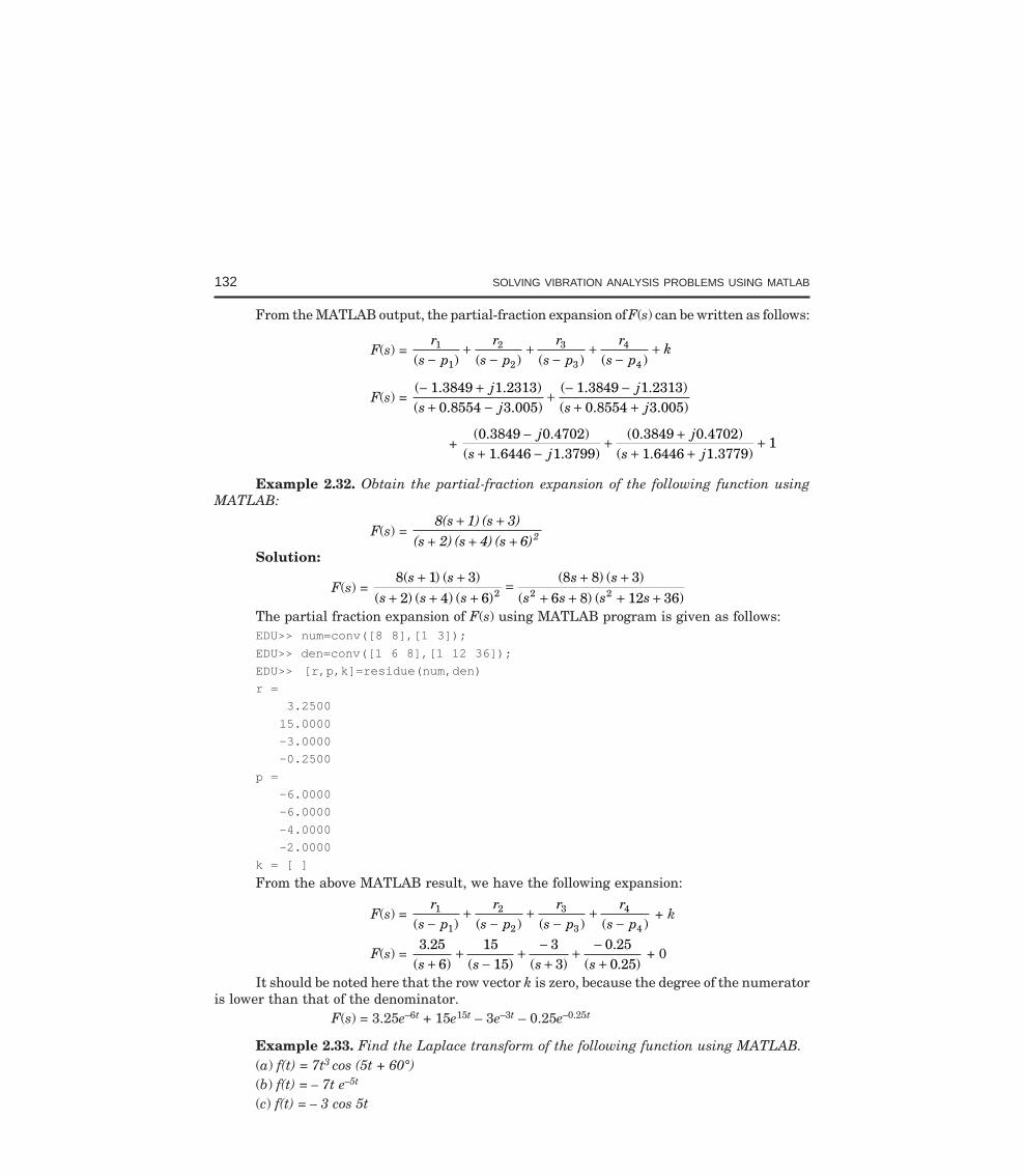
132 SOLVING VIBRATION ANALYSIS PROBLEMS USING MATLAB
From the MATLAB output, the partial-fraction expansion of F(s) can be written as follows:
F(s) = r
s pr
s pr
s pr
s pk1
1
2
2
3
3
4
4( ) ( ) ( ) ( )−+
−+
−+
−+
F(s) = ( 1.3849 1.2313)( 0.8554 3.005)
( 1.3849 1.2313)( 0.8554 3.005)
− ++ −
+ − −+ +
js j
js j
+ (0.3849 0.4702)
( 1.6446 1.3799)(0.3849 0.4702)
( 1.6446 1.3779)1
−+ −
+ ++ +
+js j
js j
Example 2.32. Obtain the partial-fraction expansion of the following function usingMATLAB:
F(s) = 8(s 1) (s 3)
(s 2) (s 4) (s 6)2+ +
+ + +Solution:
F(s) = 8 1 32 4 6
8 8 36 8 12 362 2 2
( ) ( )( ) ( ) ( )
( ) ( )( ) ( )
s ss s s
s ss s s s
+ ++ + +
= + ++ + + +
The partial fraction expansion of F(s) using MATLAB program is given as follows:EDU>> num=conv([8 8],[1 3]);
EDU>> den=conv([1 6 8],[1 12 36]);
EDU>> [r,p,k]=residue(num,den)
r =
3.2500
15.0000
-3.0000
-0.2500
p =
-6.0000
-6.0000
-4.0000
-2.0000
k = [ ]
From the above MATLAB result, we have the following expansion:
F(s) = r
s pr
s pr
s pr
s p1
1
2
2
3
3
4
4( ) ( ) ( ) ( )−+
−+
−+
− + k
F(s) = 3 25
615
1533
0 250 25
.( ) ( ) ( )
.( . )s s s s+
+−
+ −+
+ −+
+ 0
It should be noted here that the row vector k is zero, because the degree of the numeratoris lower than that of the denominator.
F(s) = 3.25e–6t + 15e15t – 3e–3t – 0.25e–0.25t
Example 2.33. Find the Laplace transform of the following function using MATLAB.(a) f(t) = 7t3 cos (5t + 60°)(b) f(t) = – 7t e–5t
(c) f(t) = – 3 cos 5t
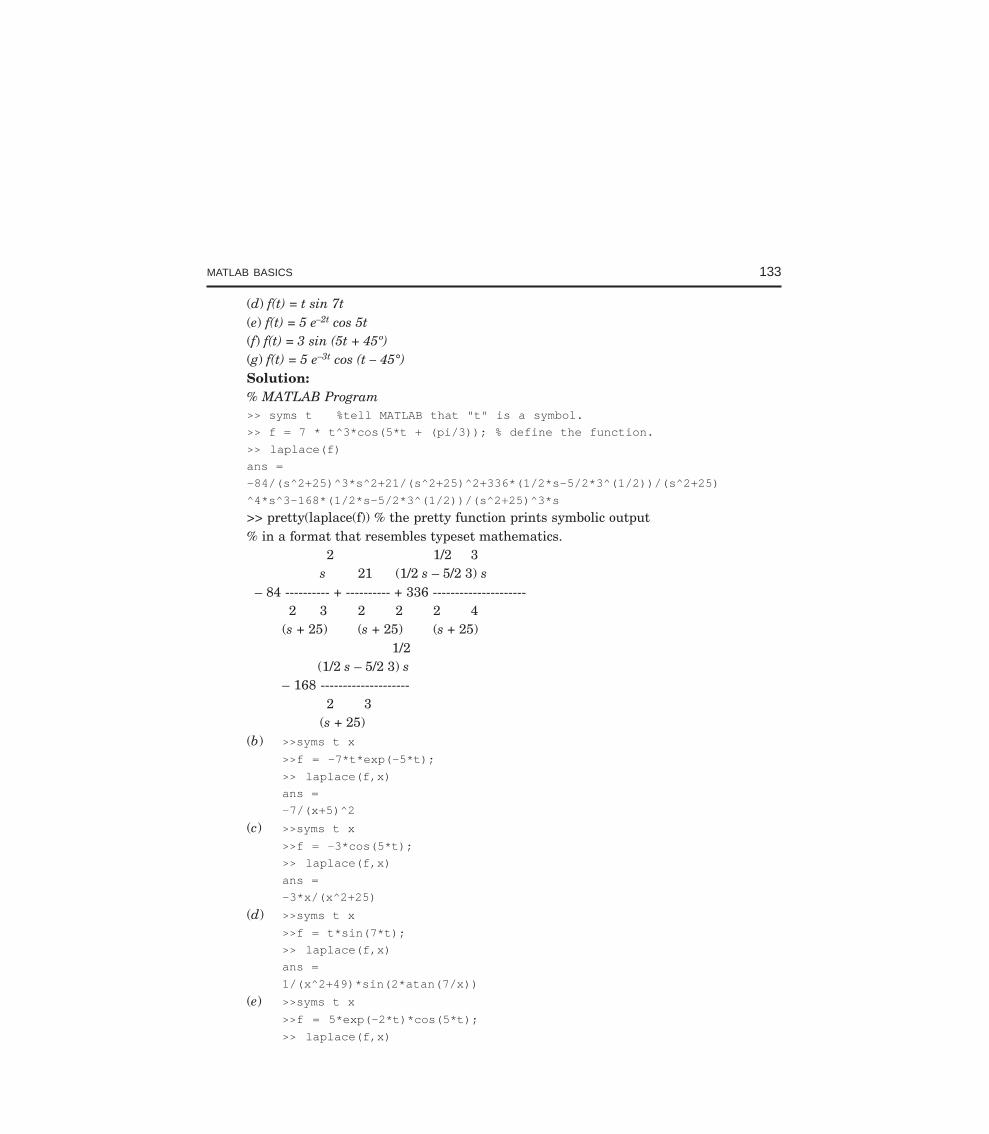
MATLAB BASICS 133
(d) f(t) = t sin 7t(e) f(t) = 5 e–2t cos 5t(f) f(t) = 3 sin (5t + 45º)(g) f(t) = 5 e–3t cos (t – 45°)Solution:% MATLAB Program>> syms t %tell MATLAB that "t" is a symbol.
>> f = 7 * t^3*cos(5*t + (pi/3)); % define the function.
>> laplace(f)
ans =
-84/(s^2+25)^3*s^2+21/(s^2+25)^2+336*(1/2*s-5/2*3^(1/2))/(s^2+25)
^4*s^3-168*(1/2*s-5/2*3^(1/2))/(s^2+25)^3*s
>> pretty(laplace(f)) % the pretty function prints symbolic output% in a format that resembles typeset mathematics.
2 1/2 3s 21 (1/2 s – 5/2 3) s
– 84 ---------- + ---------- + 336 ---------------------2 3 2 2 2 4
(s + 25) (s + 25) (s + 25) 1/2 (1/2 s – 5/2 3) s
– 168 --------------------2 3
(s + 25)(b) >>syms t x
>>f = -7*t*exp(-5*t);
>> laplace(f,x)
ans =
-7/(x+5)^2
(c) >>syms t x
>>f = -3*cos(5*t);
>> laplace(f,x)
ans =
-3*x/(x^2+25)
(d) >>syms t x
>>f = t*sin(7*t);
>> laplace(f,x)
ans =
1/(x^2+49)*sin(2*atan(7/x))
(e) >>syms t x
>>f = 5*exp(-2*t)*cos(5*t);
>> laplace(f,x)
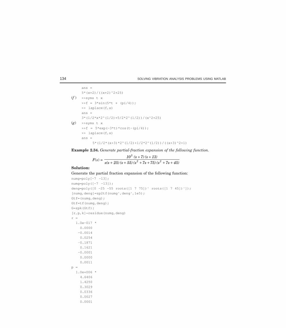
134 SOLVING VIBRATION ANALYSIS PROBLEMS USING MATLAB
ans =
5*(x+2)/((x+2)^2+25)
(f ) >>syms t x
>>f = 3*sin(5*t + (pi/4));
>> laplace(f,x)
ans =
3*(1/2*x*2^(1/2)+5/2*2^(1/2))/(x^2+25)
(g) >>syms t x
>>f = 5*exp(-3*t)*cos(t-(pi/4));
>> laplace(f,x)
ans =
5*(1/2*(x+3)*2^(1/2)+1/2*2^(1/2))/((x+3)^2+1)
Example 2.34. Generate partial-fraction expansion of the following function.
F(s) = 10 (s 7) (s 13)
s(s 25) (s 55) (s 7s 75) (s 7s 45)
5
2 2+ +
+ + + + + +Solution:Generate the partial fraction expansion of the following function:numg=poly[-7 -13];
numg=poly([-7 -13]);
deng=poly([0 -25 -55 roots([1 7 75])' roots([1 7 45])']);
[numg,deng]=zp2tf(numg',deng',1e5);
Gtf=(numg,deng);
Gtf=tf(numg,deng);
G=zpk(Gtf);
[r,p,k]=residue(numg,deng)
r =
1.0e-017 *
0.0000
-0.0014
0.0254
-0.1871
0.1621
-0.0001
0.0000
0.0011
p =
1.0e+006 *
4.6406
1.4250
0.3029
0.0336
0.0027
0.0001
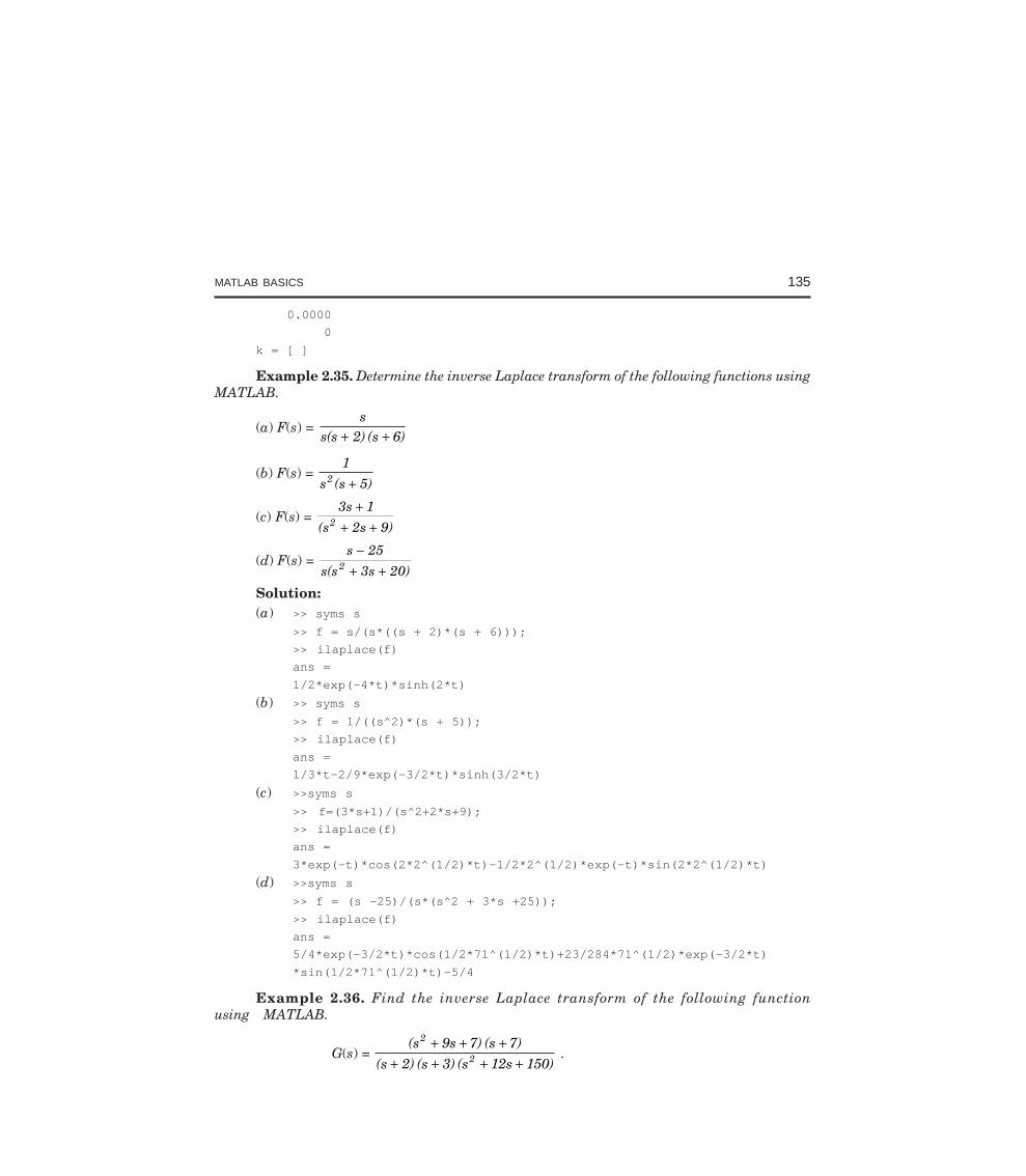
MATLAB BASICS 135
0.0000
0
k = [ ]
Example 2.35. Determine the inverse Laplace transform of the following functions usingMATLAB.
(a) F(s) = s
s(s 2) (s 6)+ +
(b) F(s) = 1
s (s 5)2 +
(c) F(s) = 3s 1
(s 2s 9)2
++ +
(d) F(s) = s 25
s(s 3s 20)2
−+ +
Solution:(a) >> syms s
>> f = s/(s*((s + 2)*(s + 6)));
>> ilaplace(f)
ans =
1/2*exp(-4*t)*sinh(2*t)
(b) >> syms s
>> f = 1/((s^2)*(s + 5));
>> ilaplace(f)
ans =
1/3*t-2/9*exp(-3/2*t)*sinh(3/2*t)
(c) >>syms s
>> f=(3*s+1)/(s^2+2*s+9);
>> ilaplace(f)
ans =
3*exp(-t)*cos(2*2^(1/2)*t)-1/2*2^(1/2)*exp(-t)*sin(2*2^(1/2)*t)
(d) >>syms s
>> f = (s -25)/(s*(s^2 + 3*s +25));
>> ilaplace(f)
ans =
5/4*exp(-3/2*t)*cos(1/2*71^(1/2)*t)+23/284*71^(1/2)*exp(-3/2*t)
*sin(1/2*71^(1/2)*t)-5/4
Example 2.36. Find the inverse Laplace transform of the following functionusing MATLAB.
G(s) = (s 9s 7) (s 7)
(s 2) (s 3) (s 12s 150)
2
2+ + +
+ + + + .
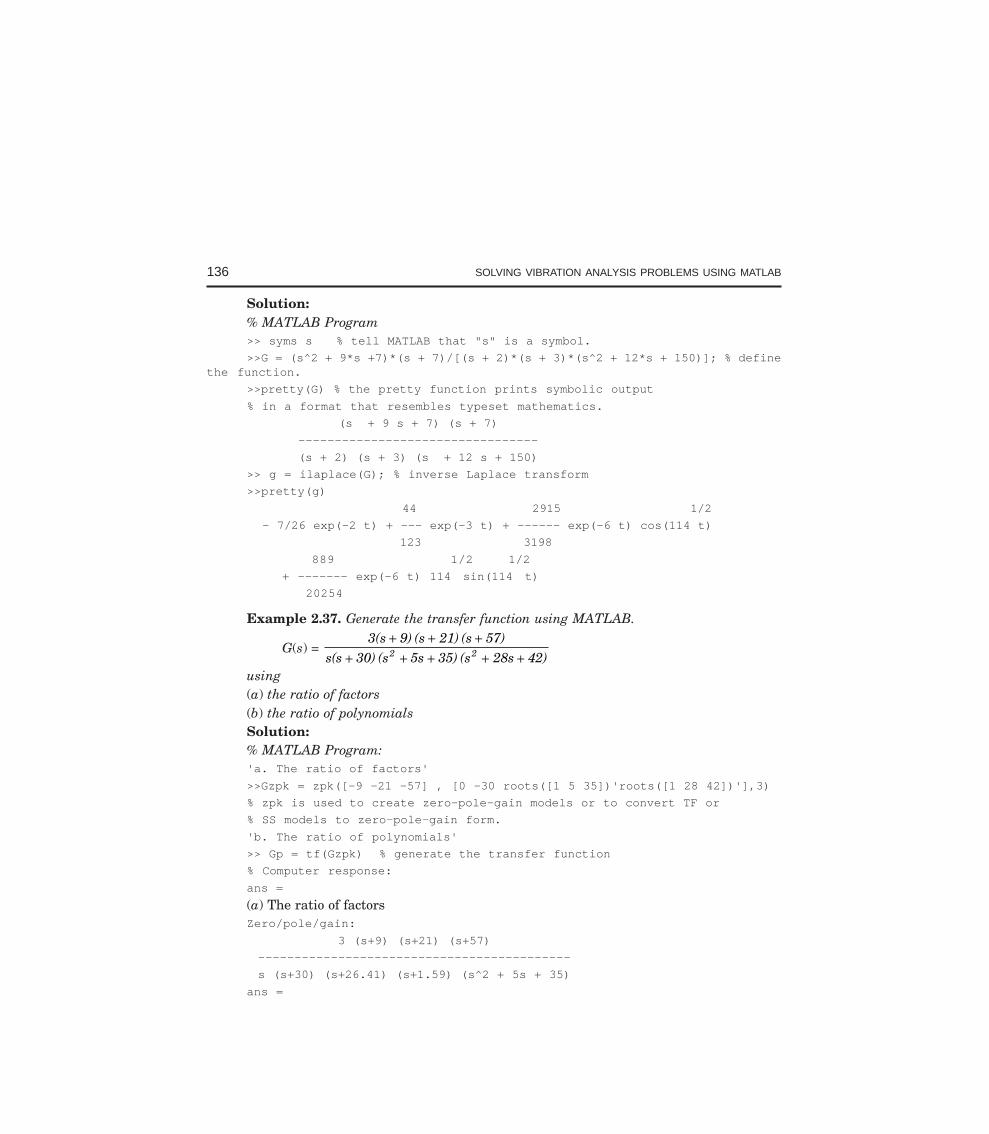
136 SOLVING VIBRATION ANALYSIS PROBLEMS USING MATLAB
Solution:% MATLAB Program>> syms s % tell MATLAB that "s" is a symbol.
>>G = (s^2 + 9*s +7)*(s + 7)/[(s + 2)*(s + 3)*(s^2 + 12*s + 150)]; % definethe function.
>>pretty(G) % the pretty function prints symbolic output
% in a format that resembles typeset mathematics.
(s + 9 s + 7) (s + 7)
---------------------------------
(s + 2) (s + 3) (s + 12 s + 150)
>> g = ilaplace(G); % inverse Laplace transform
>>pretty(g)
44 2915 1/2
- 7/26 exp(-2 t) + --- exp(-3 t) + ------ exp(-6 t) cos(114 t)
123 3198
889 1/2 1/2
+ ------- exp(-6 t) 114 sin(114 t)
20254
Example 2.37. Generate the transfer function using MATLAB.
G(s) = 3(s 9) (s 21) (s 57)
s(s 30) (s 5s 35) (s 28s 42)2 2+ + +
+ + + + +using(a) the ratio of factors(b) the ratio of polynomialsSolution:% MATLAB Program:'a. The ratio of factors'
>>Gzpk = zpk([-9 -21 -57] , [0 -30 roots([1 5 35])'roots([1 28 42])'],3)
% zpk is used to create zero-pole-gain models or to convert TF or
% SS models to zero-pole-gain form.
'b. The ratio of polynomials'
>> Gp = tf(Gzpk) % generate the transfer function
% Computer response:
ans =
(a) The ratio of factorsZero/pole/gain:
3 (s+9) (s+21) (s+57)
-------------------------------------------
s (s+30) (s+26.41) (s+1.59) (s^2 + 5s + 35)
ans =
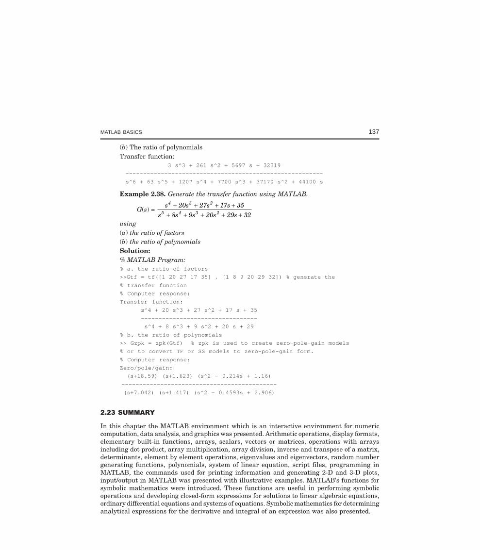
MATLAB BASICS 137
(b) The ratio of polynomialsTransfer function:
3 s^3 + 261 s^2 + 5697 s + 32319
--------------------------------------------------------
s^6 + 63 s^5 + 1207 s^4 + 7700 s^3 + 37170 s^2 + 44100 s
Example 2.38. Generate the transfer function using MATLAB.
G(s) = s 20s 27s 17s 35
s 8s 9s 20s 29s 32
4 3 2
5 4 3 2+ + + +
+ + + + +using(a) the ratio of factors(b) the ratio of polynomialsSolution:% MATLAB Program:% a. the ratio of factors
>>Gtf = tf([1 20 27 17 35] , [1 8 9 20 29 32]) % generate the
% transfer function
% Computer response:
Transfer function:
s^4 + 20 s^3 + 27 s^2 + 17 s + 35
---------------------------------
s^4 + 8 s^3 + 9 s^2 + 20 s + 29
% b. the ratio of polynomials
>> Gzpk = zpk(Gtf) % zpk is used to create zero-pole-gain models
% or to convert TF or SS models to zero-pole-gain form.
% Computer response:
Zero/pole/gain:
(s+18.59) (s+1.623) (s^2 - 0.214s + 1.16)
--------------------------------------------
(s+7.042) (s+1.417) (s^2 - 0.4593s + 2.906)
In this chapter the MATLAB environment which is an interactive environment for numericcomputation, data analysis, and graphics was presented. Arithmetic operations, display formats,elementary built-in functions, arrays, scalars, vectors or matrices, operations with arraysincluding dot product, array multiplication, array division, inverse and transpose of a matrix,determinants, element by element operations, eigenvalues and eigenvectors, random numbergenerating functions, polynomials, system of linear equation, script files, programming inMATLAB, the commands used for printing information and generating 2-D and 3-D plots,input/output in MATLAB was presented with illustrative examples. MATLAB's functions forsymbolic mathematics were introduced. These functions are useful in performing symbolicoperations and developing closed-form expressions for solutions to linear algebraic equations,ordinary differential equations and systems of equations. Symbolic mathematics for determininganalytical expressions for the derivative and integral of an expression was also presented.
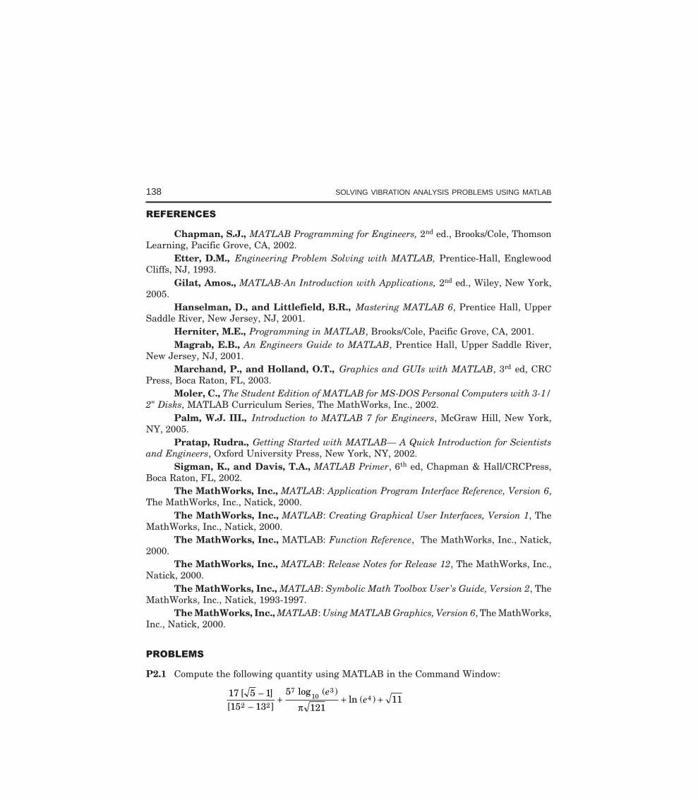
138 SOLVING VIBRATION ANALYSIS PROBLEMS USING MATLAB
Chapman, S.J., MATLAB Programming for Engineers, 2nd ed., Brooks/Cole, ThomsonLearning, Pacific Grove, CA, 2002.
Etter, D.M., Engineering Problem Solving with MATLAB, Prentice-Hall, EnglewoodCliffs, NJ, 1993.
Gilat, Amos., MATLAB-An Introduction with Applications, 2nd ed., Wiley, New York,2005.
Hanselman, D., and Littlefield, B.R., Mastering MATLAB 6, Prentice Hall, UpperSaddle River, New Jersey, NJ, 2001.
Herniter, M.E., Programming in MATLAB, Brooks/Cole, Pacific Grove, CA, 2001.Magrab, E.B., An Engineers Guide to MATLAB, Prentice Hall, Upper Saddle River,
New Jersey, NJ, 2001.Marchand, P., and Holland, O.T., Graphics and GUIs with MATLAB, 3rd ed, CRC
Press, Boca Raton, FL, 2003.Moler, C., The Student Edition of MATLAB for MS-DOS Personal Computers with 3-1/
2" Disks, MATLAB Curriculum Series, The MathWorks, Inc., 2002.Palm, W.J. III., Introduction to MATLAB 7 for Engineers, McGraw Hill, New York,
NY, 2005.Pratap, Rudra., Getting Started with MATLAB— A Quick Introduction for Scientists
and Engineers, Oxford University Press, New York, NY, 2002.Sigman, K., and Davis, T.A., MATLAB Primer, 6th ed, Chapman & Hall/CRCPress,
Boca Raton, FL, 2002.The MathWorks, Inc., MATLAB: Application Program Interface Reference, Version 6,
The MathWorks, Inc., Natick, 2000.The MathWorks, Inc., MATLAB: Creating Graphical User Interfaces, Version 1, The
MathWorks, Inc., Natick, 2000.The MathWorks, Inc., MATLAB: Function Reference, The MathWorks, Inc., Natick,
2000.The MathWorks, Inc., MATLAB: Release Notes for Release 12, The MathWorks, Inc.,
Natick, 2000.The MathWorks, Inc., MATLAB: Symbolic Math Toolbox User's Guide, Version 2, The
MathWorks, Inc., Natick, 1993-1997.The MathWorks, Inc., MATLAB: Using MATLAB Graphics, Version 6, The MathWorks,
Inc., Natick, 2000.
P2.1 Compute the following quantity using MATLAB in the Command Window:
17 5 115 13
5
12111
2 2
710
34[ ]
[ ]
log ( )ln ( )
−−
+ + +e
eπ
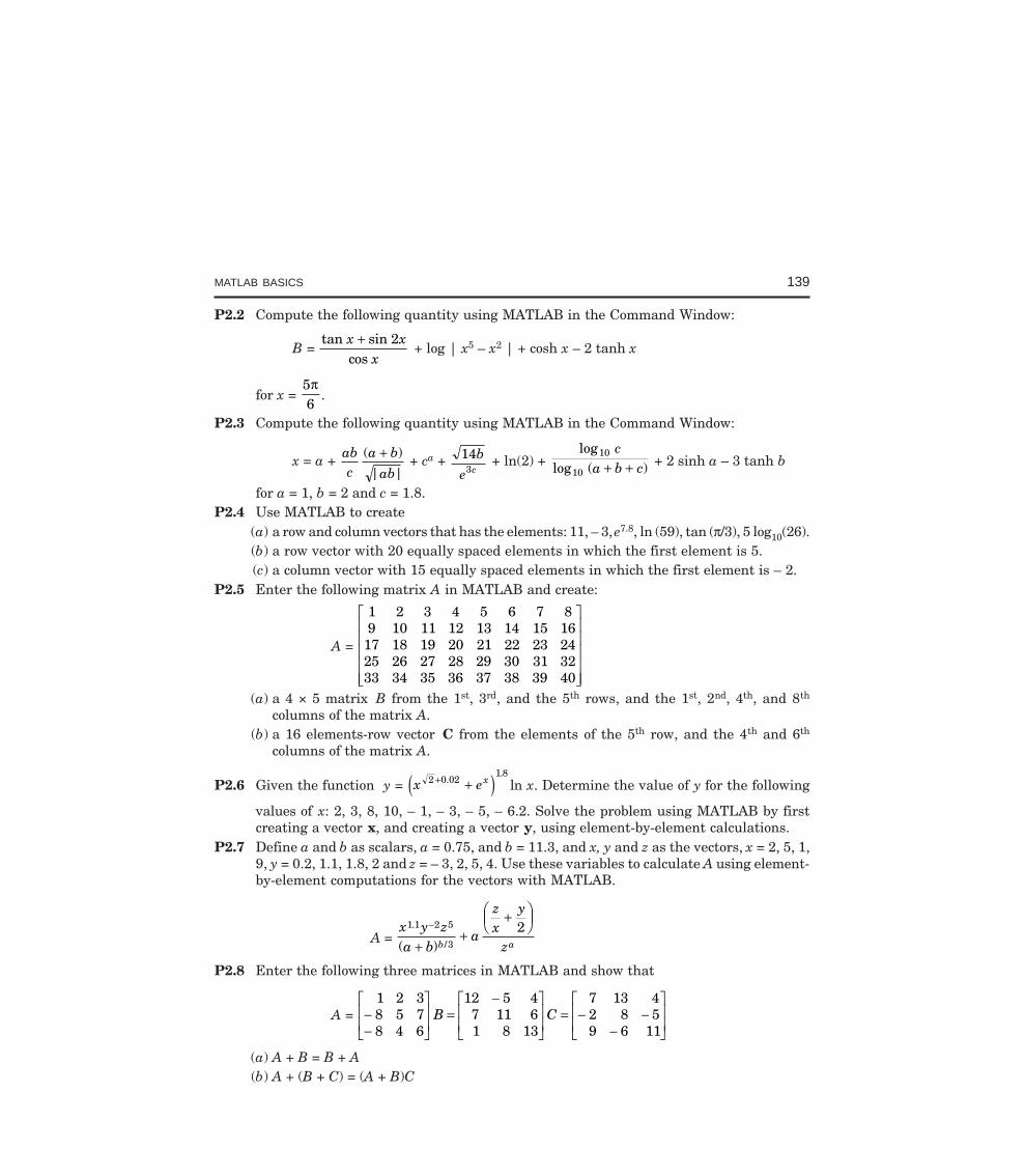
MATLAB BASICS 139
P2.2 Compute the following quantity using MATLAB in the Command Window:
B = tan sin
cosx x
x+ 2
+ log | x5 – x2 | + cosh x – 2 tanh x
for x = 56π
.
P2.3 Compute the following quantity using MATLAB in the Command Window:
x = a + abc
a b
ab
( )
| |
+ + ca + 143
b
e c + ln(2) +
loglog ( )
10
10
ca b c+ + + 2 sinh a – 3 tanh b
for a = 1, b = 2 and c = 1.8.P2.4 Use MATLAB to create
(a) a row and column vectors that has the elements: 11, – 3, e7.8, ln (59), tan (π/3), 5 log10(26).(b) a row vector with 20 equally spaced elements in which the first element is 5.(c) a column vector with 15 equally spaced elements in which the first element is – 2.
P2.5 Enter the following matrix A in MATLAB and create:
A =
1 2 3 4 5 6 7 89 10 11 12 13 14 15 16
17 18 19 20 21 22 23 2425 26 27 28 29 30 31 3233 34 35 36 37 38 39 40
L
N
MMMMM
O
Q
PPPPP
(a) a 4 × 5 matrix B from the 1st, 3rd, and the 5th rows, and the 1st, 2nd, 4th, and 8th
columns of the matrix A.(b) a 16 elements-row vector C from the elements of the 5th row, and the 4th and 6th
columns of the matrix A.
P2.6 Given the function y = x ex2 0.021 8
+ +e j.
ln x. Determine the value of y for the following
values of x: 2, 3, 8, 10, – 1, – 3, – 5, – 6.2. Solve the problem using MATLAB by firstcreating a vector x, and creating a vector y, using element-by-element calculations.
P2.7 Define a and b as scalars, a = 0.75, and b = 11.3, and x, y and z as the vectors, x = 2, 5, 1,9, y = 0.2, 1.1, 1.8, 2 and z = – 3, 2, 5, 4. Use these variables to calculate A using element-by-element computations for the vectors with MATLAB.
A = x y za b
a
zx
y
zb a
1 2 5
3
2.1
/( )
−
++
+FHG
IKJ
P2.8 Enter the following three matrices in MATLAB and show that
A = 1 2 38 5 78 4 6
12 5 47 11 61 8 13
7 13 42 8 59 6 11
−−
L
NMM
O
QPP =
−L
NMM
O
QPP = − −
−
L
NMM
O
QPPB C
(a) A + B = B + A(b) A + (B + C) = (A + B)C
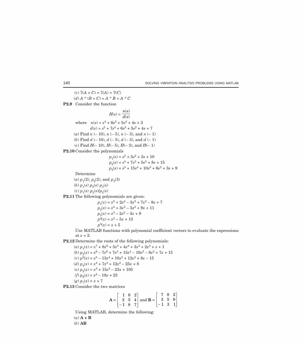
140 SOLVING VIBRATION ANALYSIS PROBLEMS USING MATLAB
(c) 7(A + C) = 7(A) + 7(C)(d) A * (B + C) = A * B + A * C
P2.9 Consider the function
H(s) = n sd s
( )( )
where n(s) = s4 + 6s3 + 5s2 + 4s + 3d(s) = s5 + 7s4 + 6s3 + 5s2 + 4s + 7
(a) Find n (– 10), n (– 5), n (– 3), and n (– 1)(b) Find d (– 10), d (– 5), d (– 3), and d (– 1)(c) Find H(– 10), H(– 5), H(– 3), and H(– 1)
P2.10 Consider the polynomialsp1(s) = s3 + 5s2 + 3s + 10p2(s) = s4 + 7s3 + 5s2 + 8s + 15p3(s) = s5 + 15s4 + 10s3 + 6s2 + 3s + 9
Determine(a) p1(2), p2(2), and p3(3)(b) p1(s) p2(s) p3(s)(c) p1(s) p2(s)/p3(s)
P2.11 The following polynomials are given:p1(x) = x5 + 2x4 – 3x3 + 7x2 – 8x + 7p2(x) = x4 + 3x3 – 5x2 + 9x + 11p3(x) = x3 – 2x2 – 3x + 9p4(x) = x2 – 5x + 13p5(x) = x + 5
Use MATLAB functions with polynomial coefficient vectors to evaluate the expressionsat x = 2.
P2.12 Determine the roots of the following polynomials:(a) p1(x) = x7 + 8x6 + 5x5 + 4x4 + 3x3 + 2x2 + x + 1(b) p2(x) = x6 – 7x6 + 7x5 + 15x4 – 10x3 – 8x2 + 7x + 15(c) p3(x) = x5 – 13x4 + 10x3 + 12x2 + 8x – 15(d) p4(x) = x4 + 7x3 + 12x2 – 25x + 8(e) p5(x) = x3 + 15x2 – 23x + 105(f) p6(x) = x2 – 18x + 23(g) p7(x) = x + 7
P2.13 Consider the two matrices
A = 1 0 22 5 41 8 7−
L
NMM
O
QPP and B =
7 8 23 5 91 3 1−
L
NMM
O
QPP
Using MATLAB, determine the following:(a) A + B(b) AB
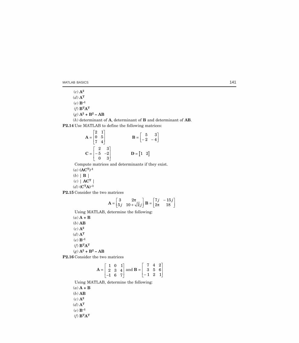
MATLAB BASICS 141
(c) A2
(d) AT
(e) B–1
(f) BTAT
(g) A2 + B2 – AB(h) determinant of A, determinant of B and determinant of AB.
P2.14 Use MATLAB to define the following matrices:
A = 2 10 57 4
L
NMM
O
QPP B =
5 32 4− −
LNM
OQP
C = 2 35 20 3
− −L
NMM
O
QPP D = 1 2
Compute matrices and determinants if they exist.(a) (ACT)-1
(b) | B |(c) | ACT |(d) (CTA)–1
P2.15 Consider the two matrices
A = 3 25 10 2
πj j+
LNM
OQP B =
7 152 18
j j−LNM
OQPπ
Using MATLAB, determine the following:(a) A + B(b) AB(c) A2
(d) AT
(e) B–1
(f) BTAT
(g) A2 + B2 – ABP2.16 Consider the two matrices
A = 1 0 12 3 41 6 7−
L
NMM
O
QPP and B =
7 4 23 5 61 2 1−
L
NMM
O
QPP
Using MATLAB, determine the following:(a) A + B(b) AB(c) A2
(d) AT
(e) B–1
(f) BTAT
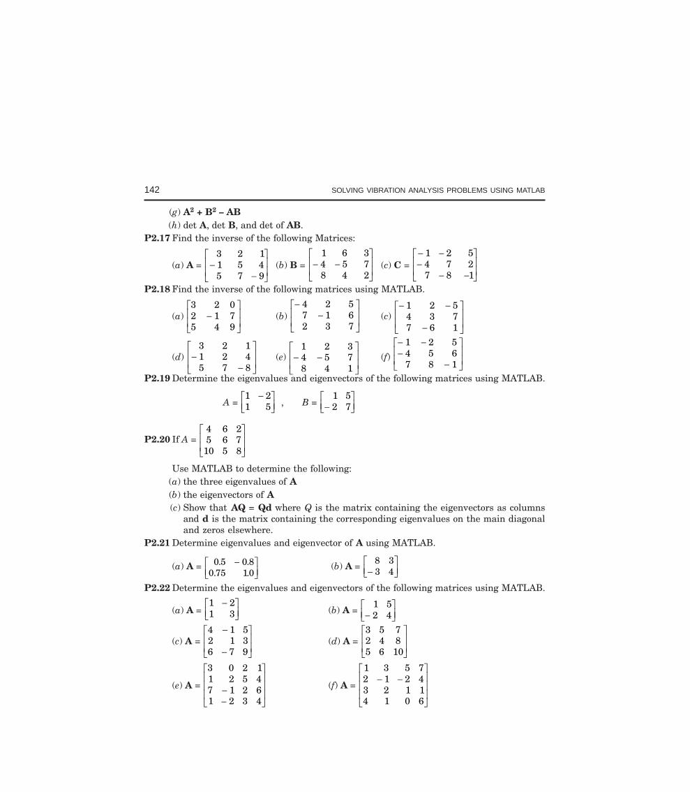
142 SOLVING VIBRATION ANALYSIS PROBLEMS USING MATLAB
(g) A2 + B2 – AB(h) det A, det B, and det of AB.
P2.17 Find the inverse of the following Matrices:
(a) A = 3 2 11 5 45 7 9
−−
L
NMM
O
QPP (b) B =
1 6 34 5 78 4 2
− −L
NMM
O
QPP (c) C =
− −−
− −
L
NMM
O
QPP
1 2 54 7 27 8 1
P2.18 Find the inverse of the following matrices using MATLAB.
(a) 3 2 02 1 75 4 9
−L
NMM
O
QPP (b)
−−
L
NMM
O
QPP
4 2 57 1 62 3 7
(c) − −
−
L
NMM
O
QPP
1 2 54 3 77 6 1
(d) 3 2 11 2 45 7 8
−−
L
NMM
O
QPP (e)
1 2 34 5 78 4 1
− −L
NMM
O
QPP (f)
− −−
−
L
NMM
O
QPP
1 2 54 5 67 8 1
P2.19 Determine the eigenvalues and eigenvectors of the following matrices using MATLAB.
A = 1 21 5
−LNM
OQP , B =
1 52 7−
LNM
OQP
P2.20 If A = 4 6 25 6 7
10 5 8
L
NMM
O
QPP
Use MATLAB to determine the following:(a) the three eigenvalues of A(b) the eigenvectors of A(c) Show that AQ = Qd where Q is the matrix containing the eigenvectors as columns
and d is the matrix containing the corresponding eigenvalues on the main diagonaland zeros elsewhere.
P2.21 Determine eigenvalues and eigenvector of A using MATLAB.
(a) A = 0 5 0 80 75 10
. .. .
−LNM
OQP
(b) A = 8 33 4−
LNM
OQP
P2.22 Determine the eigenvalues and eigenvectors of the following matrices using MATLAB.
(a) A = 1 21 3
−LNM
OQP (b) A =
1 52 4−
LNM
OQP
(c) A = 4 1 52 1 36 7 9
−
−
L
NMM
O
QPP (d) A =
3 5 72 4 85 6 10
L
NMM
O
QPP
(e) A =
3 0 2 11 2 5 47 1 2 61 2 3 4
−−
L
N
MMM
O
Q
PPP
(f) A =
1 3 5 72 1 2 43 2 1 14 1 0 6
− −L
N
MMM
O
Q
PPP
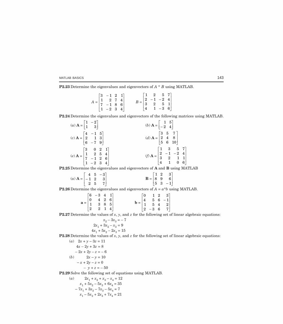
MATLAB BASICS 143
P2.23 Determine the eigenvalues and eigenvectors of A * B using MATLAB.
A =
3 1 2 11 2 7 47 1 8 61 2 3 4
−
−−
L
N
MMM
O
Q
PPP
B =
1 2 5 72 1 2 43 2 5 14 1 3 6
− −
−
L
N
MMM
O
Q
PPP
P2.24 Determine the eigenvalues and eigenvectors of the following matrices using MATLAB.
(a) A = 1 21 3
−LNM
OQP (b) A =
1 52 4−
LNM
OQP
(c) A = 4 1 52 1 36 7 9
−
−
L
NMM
O
QPP (d) A =
3 5 72 4 85 6 10
L
NMM
O
QPP
(e) A =
3 0 2 11 2 5 47 1 2 61 2 3 4
−−
L
N
MMM
O
Q
PPP
(f) A =
1 3 5 72 1 2 43 2 1 14 1 0 6
− −L
N
MMM
O
Q
PPP
P2.25 Determine the eigenvalues and eigenvectors of A and B using MATLAB
(a) A = 4 5 31 2 32 5 7
−−L
NMM
O
QPP
B = 1 2 38 9 65 3 1−
L
NMM
O
QPP
P2.26 Determine the eigenvalues and eigenvectors of A = a*b using MATLAB.
a =
6 3 4 10 4 2 61 3 8 52 2 1 4
−L
N
MMM
O
Q
PPP
b =
0 1 2 34 5 6 11 5 4 22 3 6 7
−
−
L
N
MMM
O
Q
PPP
P2.27 Determine the values of x, y, and z for the following set of linear algebraic equations:x2 – 3x3 = – 7
2x1 + 3x2 – x3 = 94x1 + 5x2 – 2x3 = 15
P2.28 Determine the values of x, y, and z for the following set of linear algebraic equations:(a) 2x + y – 3z = 11
4x – 2y + 3z = 8– 2x + 2y – z = – 6
(b) 2x – y = 10– x + 2y – z = 0
– y + z = – 50P2.29 Solve the following set of equations using MATLAB.
(a) 2x1 + x2 + x3 – x4 = 12x1 + 5x2 – 5x3 + 6x4 = 35
– 7x1 + 3x2 – 7x3 – 5x4 = 7x1 – 5x2 + 2x3 + 7x4 = 21
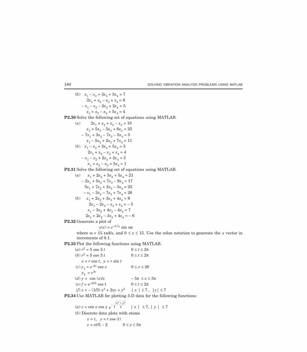
144 SOLVING VIBRATION ANALYSIS PROBLEMS USING MATLAB
(b) x1 – x2 + 3x3 + 5x4 = 72x1 + x2 – x3 + x4 = 6
– x1 – x2 – 2x3 + 2x4 = 5x1 + x2 – x3 + 5x4 = 4
P2.30 Solve the following set of equations using MATLAB.(a) 2x1 + x2 + x3 – x4 = 10
x1 + 5x2 – 5x3 + 6x4 = 25– 7x1 + 3x2 – 7x3 – 5x4 = 5
x1 – 5x2 + 2x3 + 7x4 = 11(b) x1 – x2 + 3x3 + 5x4 = 5
2x1 + x2 – x3 + x4 = 4– x1 – x2 + 2x3 + 2x4 = 3
x1 + x2 – x3 + 5x4 = 1P2.31 Solve the following set of equations using MATLAB.
(a) x1 + 2x2 + 3x3 + 5x4 = 21– 2x1 + 5x2 + 7x3 – 9x4 = 17
5x1 + 7x2 + 2x3 – 5x4 = 23– x1 – 3x2 – 7x3 + 7x4 = 26
(b) x1 + 2x2 + 3x3 + 4x4 = 9 2x1 – 2x2 – x3 + x4 = – 5x1 – 3x2 + 4x3 – 4x4 = 7
2x1 + 2x2 – 3x3 + 4x4 = – 6P2.32 Generate a plot of
y(x) = e–0.7x sin ωxwhere ω = 15 rad/s, and 0 ≤ x ≤ 15. Use the colon notation to generate the x vector inincrements of 0.1.
P2.33 Plot the following functions using MATLAB.(a) r2 = 5 cos 3 t 0 ≤ t ≤ 2π(b) r2 = 5 cos 3 t 0 ≤ t ≤ 2π
x = r cos t, y = r sin t(c) y1 = e–2x cos x 0 ≤ x ≤ 20
y2 = e2x
(d) y = cos (x)/x – 5π ≤ x ≤ 5π(e) f = e–3t/5 cos t 0 ≤ t ≤ 2π(f) z = – (1/3) x2 + 2xy + y2 | x | ≤ 7 , |y| ≤ 7
P2.34 Use MATLAB for plotting 3-D data for the following functions:
(a) z = cos x cos y ex y−
+2 2
5 | x | ≤ 7, | y | ≤ 7
(b) Discrete data plots with stemsx = t, y = t cos (t)z = et/5 – 2 0 ≤ x ≤ 5π
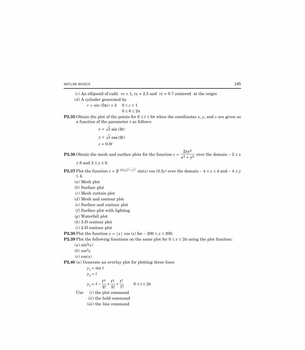
MATLAB BASICS 145
(c) An ellipsoid of radii rx = 1, ry = 2.5 and rz = 0.7 centered at the origin(d) A cylinder generated by
r = sin (5πz) + 3 0 ≤ z ≤ 10 ≤ θ ≤ 2π
P2.35 Obtain the plot of the points for 0 ≤ t ≤ 6π when the coordinates x, y, and z are given asa function of the parameter t as follows:
x = t tsin ( )3
y = t tcos ( )3
z = 0.8t
P2.36 Obtain the mesh and surface plots for the function z = 2 2
2 2
xyx y+
over the domain – 2 ≤ x
≤ 6 and 2 ≤ y ≤ 8.
P2.37 Plot the function z = 2 1 5 2 2− +. x y sin(x) cos (0.5y) over the domain – 4 ≤ x ≤ 4 and – 4 ≤ y≤ 4.
(a) Mesh plot(b) Surface plot(c) Mesh curtain plot(d) Mesh and contour plot(e) Surface and contour plot(f) Surface plot with lighting(g) Waterfall plot(h) 3-D contour plot(i) 2-D contour plot
P2.38 Plot the function y = |x| cos (x) for – 200 ≤ x ≤ 200.P2.39 Plot the following functions on the same plot for 0 ≤ x ≤ 2π using the plot function:
(a) sin2(x)(b) cos2x(c) cos(x)
P2.40 (a) Generate an overlay plot for plotting three linesy1 = sin ty2 = t
y3 = tt t t
− + +3 5 7
3 5 7! ! !0 ≤ t ≤ 2π
Use (i) the plot command (ii) the hold command(iii) the line command
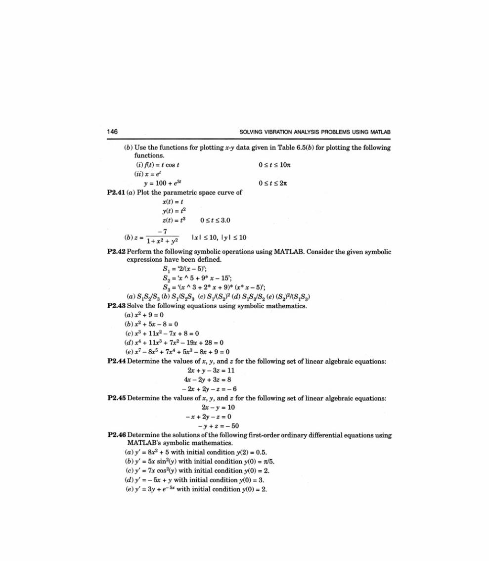
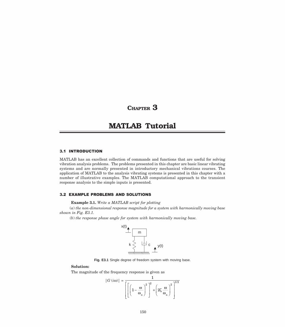
CHAPTER 3
MATLAB Tutorial
MATLAB has an excellent collection of commands and functions that are useful for solvingvibration analysis problems. The problems presented in this chapter are basic linear vibratingsystems and are normally presented in introductory mechanical vibrations courses. Theapplication of MATLAB to the analysis vibrating systems is presented in this chapter with anumber of illustrative examples. The MATLAB computational approach to the transientresponse analysis to the simple inputs is presented.
Example 3.1. Write a MATLAB script for plotting(a) the non-dimensional response magnitude for a system with harmonically moving base
shown in Fig. E3.1.(b) the response phase angle for system with harmonically moving base.
m
k c
x(t)
y(t)
Fig. E3.1 Single degree of freedom system with moving base.
Solution:The magnitude of the frequency response is given as
|G (iω)| = 1
1 22 2 2
1/2
−FHG
IKJ
L
NMM
O
QPP +
FHG
IKJ
L
N
MMM
O
Q
PPP
ωω
ζ ωωn n
150
MATLAB TUTORIAL 151
The magnitude of X (iω) is given as
|X (iω)| = 12
2 1/2
+FHG
IKJ
L
NMM
O
QPP
ζωω n
|G (iω) |A
where y (t) = Re Aiωt
x (t) = X (iω) eiωt
The phase angle φ is given as
φ(ω) = tan–1
2
12
3
2 2
ζ ωω
ωω
ζωω
n
n n
FHG
IKJ
−FHG
IKJ +
FHG
IKJ
L
N
MMMMM
O
Q
PPPPP
The frequency ratio
r = ω
ωn
The non-dimensional response magnitude is given as the transmissibility
| ( )|X iA
ω =
12
12
2
2 2
+FHG
IKJ
−FHG
IKJ +
FHG
IKJ
L
N
MMMMM
O
Q
PPPPP
ζωω
ωω
ζωω
n
n n
Based on these equations MATLAB script is written as follows:zeta= [0.05; 0.1; 0.15; 0.25; 0.5; 1.25; 1.5]; % damping factors
r= [0:0.01:3]; %frequency ratio
for k=1: length (zeta)
G(k,:)=sqrt((1+(2*zeta(k)*r).^2)./((1-r.^2).^2+(2*zeta(k)*r).^2));
phi(k,:)=atan2(2*zeta(k)*r.^3,1-r.^2+(2*zeta(k)*r).^2);
end
figure (1)
plot(r, G)
xlabel ('\omega/\omega_n')
ylabel ('|x (i\omega)|/A')
grid
legend ('\zeta_1=0.05','\zeta_2=0.1','\zeta_3=0.15','\zeta_4
=0.25','\zeta_5=0.5','\zeta_6=1.25','\zeta_7=1.5')
figure (2)
plot(r, phi)
xlabel ('\omega/\omega_n')
ylabel ('\phi (\omega)')
grid
ha=gca;
set (ha,'ytick',[0:pi/2:pi])
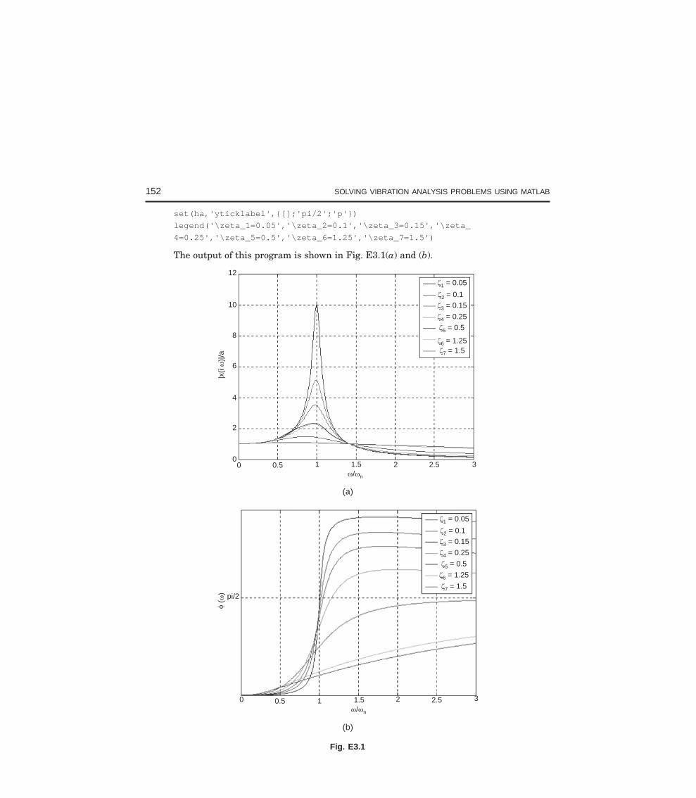
152 SOLVING VIBRATION ANALYSIS PROBLEMS USING MATLAB
set(ha,'yticklabel',[];'pi/2';'p')
legend('\zeta_1=0.05','\zeta_2=0.1','\zeta_3=0.15','\zeta_
4=0.25','\zeta_5=0.5','\zeta_6=1.25','\zeta_7=1.5')
The output of this program is shown in Fig. E3.1(a) and (b).
12
10
8
6
4
2
00 0.5 1 1.5 2 2.5 3
/n
|x(i
)|/a
1 = 0.05
2 = 0.1
3 = 0.15
4 = 0.25
5 = 0.5
6 = 1.257 = 1.5
(a)
(
) pi/2
0 1 1.5 20.5 2.5 3
/ n
1 = 0.05
2 = 0.1
3 = 0.15
4 = 0.25
5 = 0.5
6 = 1.25
7 = 1.5
(b)
Fig. E3.1
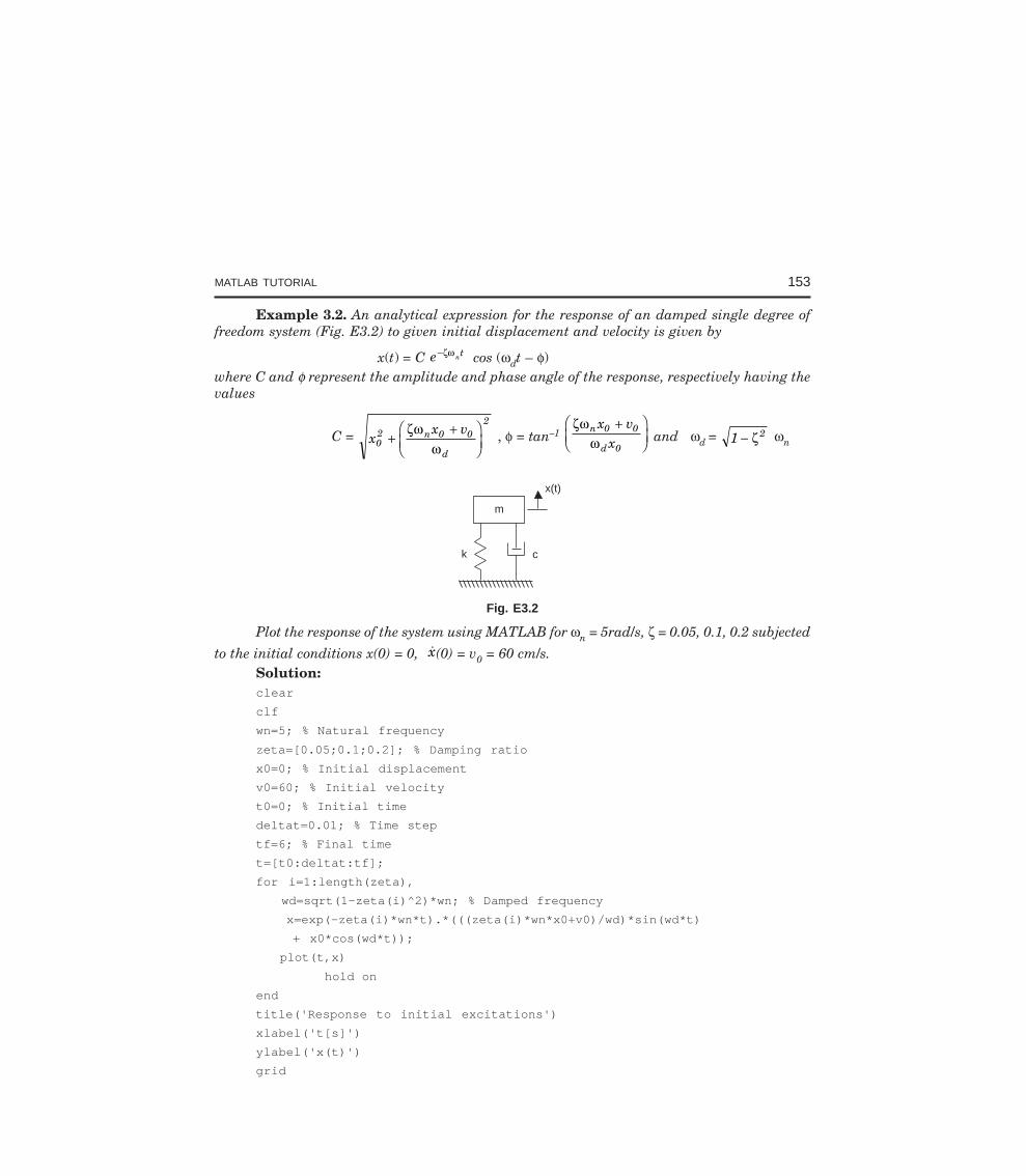
MATLAB TUTORIAL 153
Example 3.2. An analytical expression for the response of an damped single degree offreedom system (Fig. E3.2) to given initial displacement and velocity is given by
x(t) = C e nt−ζω cos (ωdt – φ)where C and φ represent the amplitude and phase angle of the response, respectively having thevalues
C = xx v
02 n 0 0
d
2
++F
HGIKJ
ζωω
, φ = tan–1 ζω
ωn 0 0
d 0
x vx+F
HGIKJ and ωd = 1 2− ζ ωn
m
k
x(t)
c
Fig. E3.2
Plot the response of the system using MATLAB for ωn = 5rad/s, ζ = 0.05, 0.1, 0.2 subjected
to the initial conditions x(0) = 0, x(0) = v0 = 60 cm/s.Solution:clear
clf
wn=5; % Natural frequency
zeta=[0.05;0.1;0.2]; % Damping ratio
x0=0; % Initial displacement
v0=60; % Initial velocity
t0=0; % Initial time
deltat=0.01; % Time step
tf=6; % Final time
t=[t0:deltat:tf];
for i=1:length(zeta),
wd=sqrt(1-zeta(i)^2)*wn; % Damped frequency
x=exp(-zeta(i)*wn*t).*(((zeta(i)*wn*x0+v0)/wd)*sin(wd*t)
+ x0*cos(wd*t));
plot(t,x)
hold on
end
title('Response to initial excitations')
xlabel('t[s]')
ylabel('x(t)')
grid
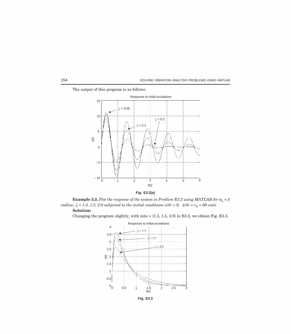
154 SOLVING VIBRATION ANALYSIS PROBLEMS USING MATLAB
The output of this program is as follows:
Response to initial excitations15
10
5
0
– 5
– 100 1 2 3 4 5 6
t[s]
= 0.05
= 0.1
= 0.2
Fig. E3.2(a)
Example 3.3. Plot the response of the system in Problem E3.2 using MATLAB for ωn = 5rad/sec, ζ = 1.3, 1.5, 2.0 subjected to the initial conditions x(0) = 0, x(0) = v0 = 60 cm/s.
Solution:Changing the program slightly, with zeta = [1.3, 1.5, 2.0] in E3.2, we obtain Fig. E3.3.
Response to initial excitations
3.5
3
2.5
2
1.5
1
0.5
0
4
x(t)
0 0.5 1 21.5 2.5 3t[s]
Fig. E3.3
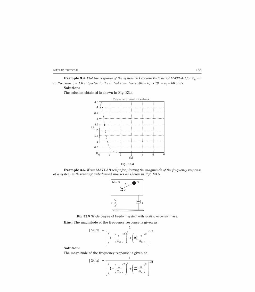
MATLAB TUTORIAL 155
Example 3.4. Plot the response of the system in Problem E3.2 using MATLAB for ωn = 5rad/sec and ζ = 1.0 subjected to the initial conditions x(0) = 0, x(0) = v0 = 60 cm/s.
Solution:The solution obtained is shown in Fig. E3.4.
Response to initial excitations4.5
4
3.5
3
2.5
2
1.5
1
0.5
0
x(t)
0 1 2 3 4 5 6t[s]
Fig. E3.4
Example 3.5. Write MATLAB script for plotting the magnitude of the frequency responseof a system with rotating unbalanced masses as shown in Fig. E3.5.
M – m
k c
me
Fig. E3.5 Single degree of freedom system with rotating eccentric mass.
Hint: The magnitude of the frequency response is given as
|G(iω)| = 1
1 22 2 2
1/2
−FHG
IKJ
FHGG
IKJJ +
FHG
IKJ
L
NMMM
O
QPPP
ωω
ζ ωωn n
Solution:The magnitude of the frequency response is given as
|G(iω)| = 1
1 22 2 2
1/2
−FHG
IKJ
FHGG
IKJJ +
FHG
IKJ
L
NMMM
O
QPPP
ωω
ζ ωωn n
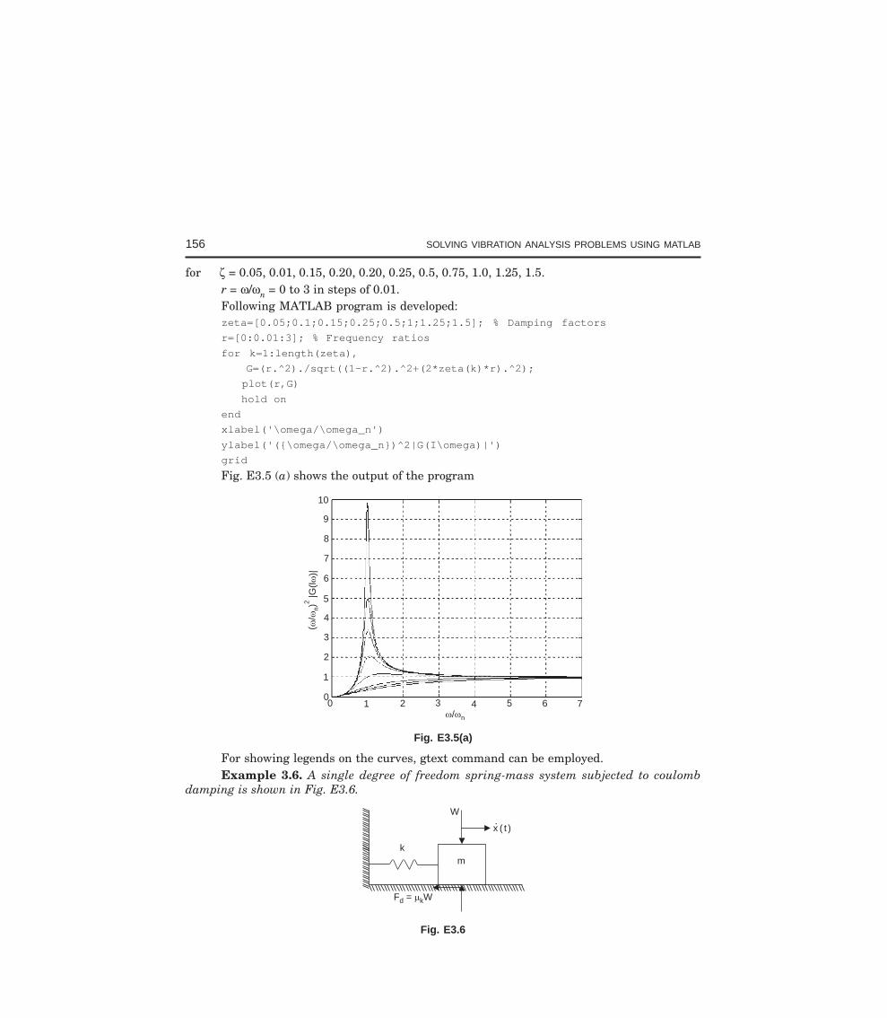
156 SOLVING VIBRATION ANALYSIS PROBLEMS USING MATLAB
for ζ = 0.05, 0.01, 0.15, 0.20, 0.20, 0.25, 0.5, 0.75, 1.0, 1.25, 1.5.r = ω/ωn = 0 to 3 in steps of 0.01.Following MATLAB program is developed:zeta=[0.05;0.1;0.15;0.25;0.5;1;1.25;1.5]; % Damping factors
r=[0:0.01:3]; % Frequency ratios
for k=1:length(zeta),
G=(r.^2)./sqrt((1-r.^2).^2+(2*zeta(k)*r).^2);
plot(r,G)
hold on
end
xlabel('\omega/\omega_n')
ylabel('(\omega/\omega_n)^2|G(I\omega)|')
grid
Fig. E3.5 (a) shows the output of the program
(/
)|G
(l)|
n
2
10
9
8
7
6
5
4
3
2
1
00 1 2 3 4 5 6 7
/ n
Fig. E3.5(a)
For showing legends on the curves, gtext command can be employed.Example 3.6. A single degree of freedom spring-mass system subjected to coulomb
damping is shown in Fig. E3.6.
mk
W
)t(x
F = Wd k
Fig. E3.6
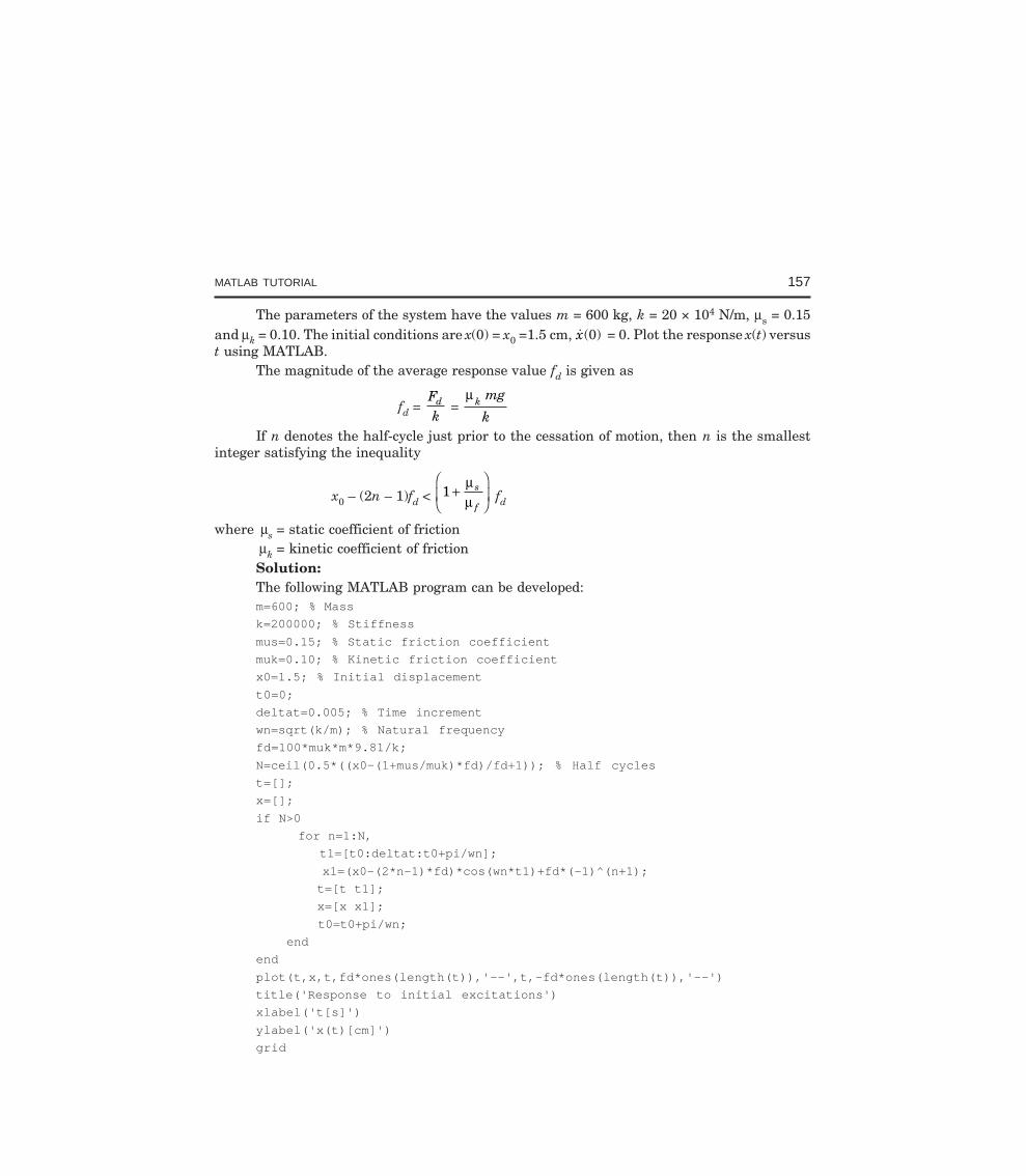
MATLAB TUTORIAL 157
The parameters of the system have the values m = 600 kg, k = 20 × 104 N/m, µs = 0.15and µk = 0.10. The initial conditions are x(0) = x0 =1.5 cm, x(0) = 0. Plot the response x(t) versust using MATLAB.
The magnitude of the average response value fd is given as
fd = Fkd =
µ k mg
kIf n denotes the half-cycle just prior to the cessation of motion, then n is the smallest
integer satisfying the inequality
x0 – (2n – 1)fd < 1 +FHG
IKJ
µµ
s
f fd
where µs = static coefficient of frictionµk = kinetic coefficient of frictionSolution:The following MATLAB program can be developed:m=600; % Mass
k=200000; % Stiffness
mus=0.15; % Static friction coefficient
muk=0.10; % Kinetic friction coefficient
x0=1.5; % Initial displacement
t0=0;
deltat=0.005; % Time increment
wn=sqrt(k/m); % Natural frequency
fd=100*muk*m*9.81/k;
N=ceil(0.5*((x0-(1+mus/muk)*fd)/fd+1)); % Half cycles
t=[];
x=[];
if N>0
for n=1:N,
t1=[t0:deltat:t0+pi/wn];
x1=(x0-(2*n-1)*fd)*cos(wn*t1)+fd*(-1)^(n+1);
t=[t t1];
x=[x x1];
t0=t0+pi/wn;
end
end
plot(t,x,t,fd*ones(length(t)),'--',t,-fd*ones(length(t)),'--')
title('Response to initial excitations')
xlabel('t[s]')
ylabel('x(t)[cm]')
grid
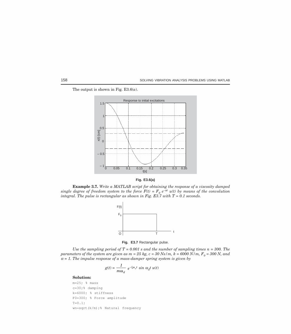
158 SOLVING VIBRATION ANALYSIS PROBLEMS USING MATLAB
The output is shown in Fig. E3.6(a).
1.5
1
Response to initial excitations
0.5
0
– 0.5
– 1
0
0.05 0.1 0.15 0.2 0.25 0.3 0.35t[s]
x(t)
[cm
]
Fig. E3.6(a)
Example 3.7. Write a MATLAB script for obtaining the response of a viscosity dampedsingle degree of freedom system to the force F(t) = F0 e–αt u(t) by means of the convolutionintegral. The pulse is rectangular as shown in Fig. E3.7 with T = 0.1 seconds.
tTO
F0
F(t)
Fig. E3.7 Rectangular pulse.
Use the sampling period of T = 0.001 s and the number of sampling times n = 300. Theparameters of the system are given as m = 25 kg, c = 30 Ns/m, k = 6000 N/m, F0 = 300 N, andα = 1. The impulse response of a mass-damper spring system is given by
g(t) = 1
m dω e nt−ζω sin ωdt u(t)
Solution:m=25; % mass
c=30;% damping
k=6000; % stiffness
F0=300; % Force amplitude
T=0.1;
wn=sqrt(k/m);% Natural frequency
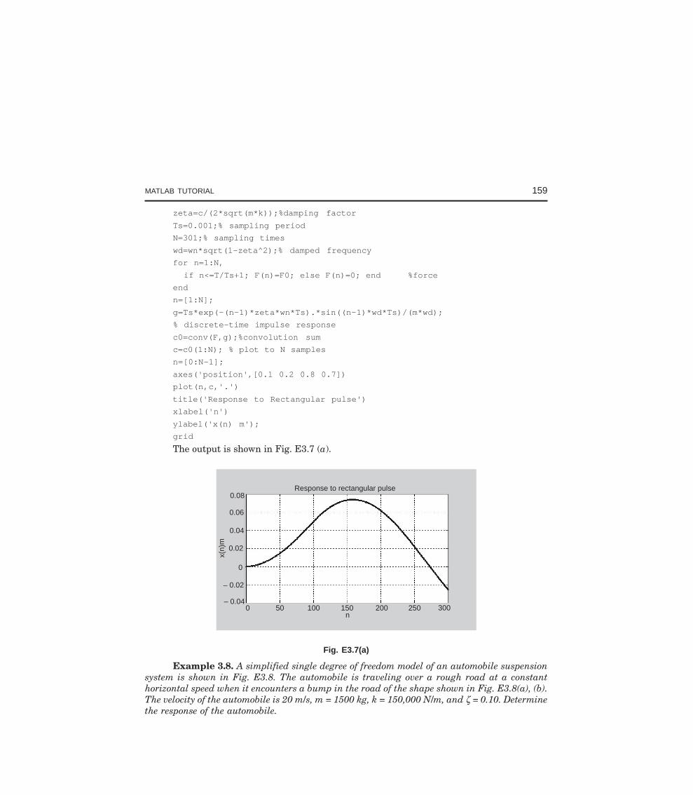
MATLAB TUTORIAL 159
zeta=c/(2*sqrt(m*k));%damping factor
Ts=0.001;% sampling period
N=301;% sampling times
wd=wn*sqrt(1-zeta^2);% damped frequency
for n=1:N,
if n<=T/Ts+1; F(n)=F0; else F(n)=0; end %force
end
n=[1:N];
g=Ts*exp(-(n-1)*zeta*wn*Ts).*sin((n-1)*wd*Ts)/(m*wd);
% discrete-time impulse response
c0=conv(F,g);%convolution sum
c=c0(1:N); % plot to N samples
n=[0:N-1];
axes('position',[0.1 0.2 0.8 0.7])
plot(n,c,'.')
title('Response to Rectangular pulse')
xlabel('n')
ylabel('x(n) m');
grid
The output is shown in Fig. E3.7 (a).
Response to rectangular pulse0.08
0.06
0.04
0.02
0
– 0.02
– 0.040 50 100 200 300150 250
x(n)
m
n
Fig. E3.7(a)
Example 3.8. A simplified single degree of freedom model of an automobile suspensionsystem is shown in Fig. E3.8. The automobile is traveling over a rough road at a constanthorizontal speed when it encounters a bump in the road of the shape shown in Fig. E3.8(a), (b).The velocity of the automobile is 20 m/s, m = 1500 kg, k = 150,000 N/m, and ζ = 0.10. Determinethe response of the automobile.
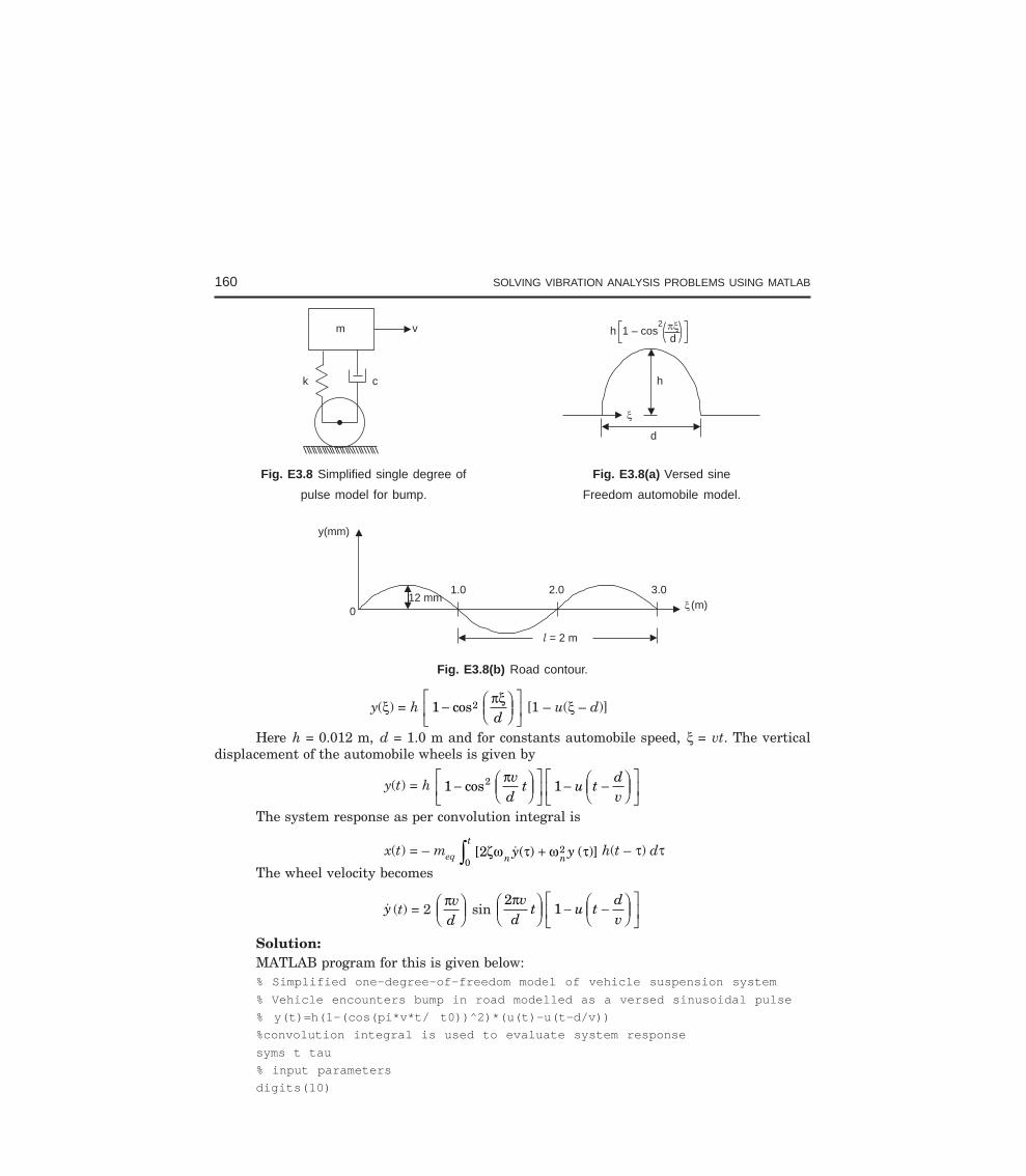
160 SOLVING VIBRATION ANALYSIS PROBLEMS USING MATLAB
m
k c
v
h
d
h 1 – cos2
d
Fig. E3.8 Simplified single degree of Fig. E3.8(a) Versed sine
pulse model for bump. Freedom automobile model.
12 mm0
1.0 2.0 3.0
= 2 ml
(m)
y(mm)
Fig. E3.8(b) Road contour.
y(ξ) = h 1 2− FHG
IKJ
LNM
OQP
cosπξd
[1 – u(ξ – d)]
Here h = 0.012 m, d = 1.0 m and for constants automobile speed, ξ = vt. The verticaldisplacement of the automobile wheels is given by
y(t) = h 1 12− FHG
IKJ
LNM
OQP
− −FHG
IKJ
LNM
OQP
cosπvd
t u tdv
The system response as per convolution integral is
x(t) = – meq 0
22t
n ny yz +[ ( ) ( )]ζω τ ω τ h(t – τ) dτ
The wheel velocity becomes
y (t) = 2 πvd
FHG
IKJ sin
21
πvd
t u tdv
FHG
IKJ − −F
HGIKJ
LNM
OQP
Solution:MATLAB program for this is given below:% Simplified one-degree-of-freedom model of vehicle suspension system
% Vehicle encounters bump in road modelled as a versed sinusoidal pulse
% y(t)=h(1-(cos(pi*v*t/ t0))^2)*(u(t)-u(t-d/v))
%convolution integral is used to evaluate system response
syms t tau
% input parameters
digits(10)
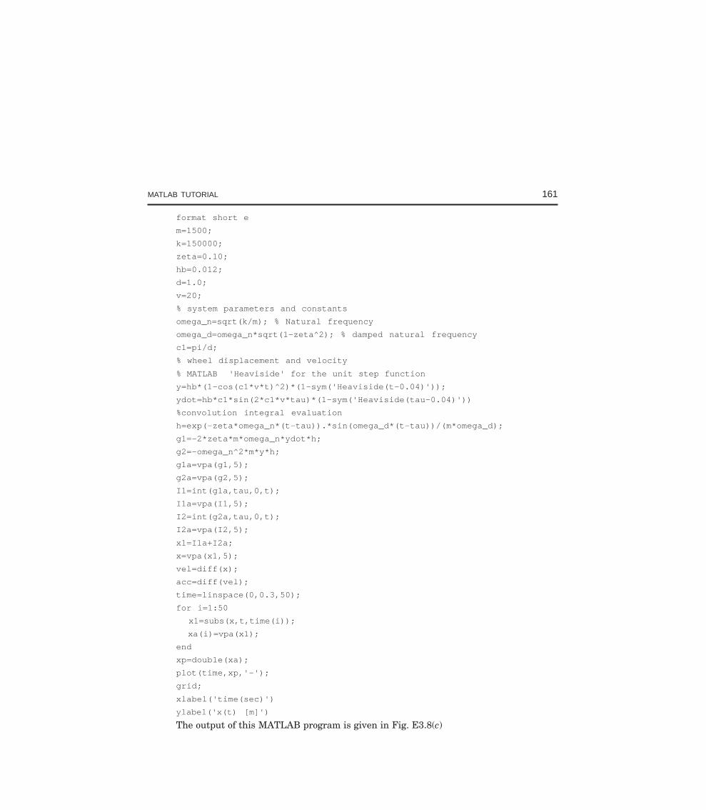
MATLAB TUTORIAL 161
format short e
m=1500;
k=150000;
zeta=0.10;
hb=0.012;
d=1.0;
v=20;
% system parameters and constants
omega_n=sqrt(k/m); % Natural frequency
omega_d=omega_n*sqrt(1-zeta^2); % damped natural frequency
c1=pi/d;
% wheel displacement and velocity
% MATLAB 'Heaviside' for the unit step function
y=hb*(1-cos(c1*v*t)^2)*(1-sym('Heaviside(t-0.04)'));
ydot=hb*c1*sin(2*c1*v*tau)*(1-sym('Heaviside(tau-0.04)'))
%convolution integral evaluation
h=exp(-zeta*omega_n*(t-tau)).*sin(omega_d*(t-tau))/(m*omega_d);
g1=-2*zeta*m*omega_n*ydot*h;
g2=-omega_n^2*m*y*h;
g1a=vpa(g1,5);
g2a=vpa(g2,5);
I1=int(g1a,tau,0,t);
I1a=vpa(I1,5);
I2=int(g2a,tau,0,t);
I2a=vpa(I2,5);
x1=I1a+I2a;
x=vpa(x1,5);
vel=diff(x);
acc=diff(vel);
time=linspace(0,0.3,50);
for i=1:50
x1=subs(x,t,time(i));
xa(i)=vpa(x1);
end
xp=double(xa);
plot(time,xp,'-');
grid;
xlabel('time(sec)')
ylabel('x(t) [m]')
The output of this MATLAB program is given in Fig. E3.8(c)
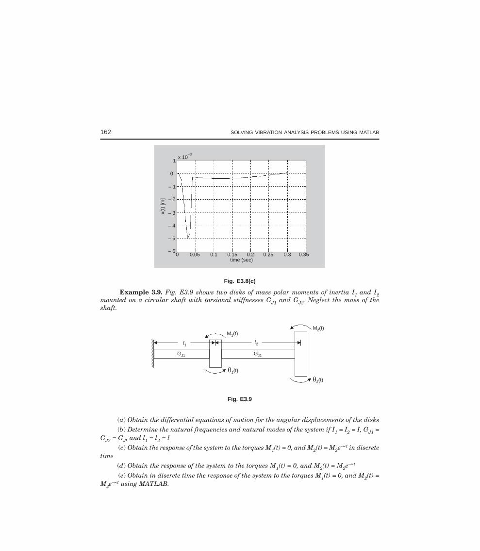
162 SOLVING VIBRATION ANALYSIS PROBLEMS USING MATLAB
x 10–3
1
0
– 1
– 2
– 3
– 4
– 5
– 6
x(t)
[m]
0 0.05 0.1 0.15 0.2 0.25 0.3 0.35time (sec)
Fig. E3.8(c)
Example 3.9. Fig. E3.9 shows two disks of mass polar moments of inertia I1 and I2mounted on a circular shaft with torsional stiffnesses GJ1 and GJ2. Neglect the mass of theshaft.
GJ1 GJ2
l1l2
M (t)1
1(t)
2(t)
M (t)2
Fig. E3.9
(a) Obtain the differential equations of motion for the angular displacements of the disks(b) Determine the natural frequencies and natural modes of the system if I1 = I2 = I, GJ1 =
GJ2 = GJ, and l1 = l2 = l
(c) Obtain the response of the system to the torques M1(t) = 0, and M2(t) = M2e–∝t in discretetime
(d) Obtain the response of the system to the torques M1(t) = 0, and M2(t) = M2e–∝t
(e) Obtain in discrete time the response of the system to the torques M1(t) = 0, and M2(t) =M2e
–∝t using MATLAB.
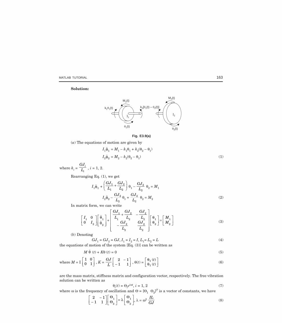
MATLAB TUTORIAL 163
Solution:
I1
1(t) 2(t)
k11(t)
I2
M (t)1
k [ (t) – (t)]2 1 2
M (t)2
Fig. E3.9(a)
(a) The equations of motion are given by
I1θ1 = M1 – k1θ1 + k2(θ2 – θ1)
I2θ2 = M2 – k2(θ2 – θ1) (1)
where ki = GJL
i
i , i = 1, 2.
Rearranging Eq. (1), we get
I1θ1 +
GJL
GJL
1
1
2
2+
FHG
IKJ θ1 –
GJL
2
2 θ2 = M1
I2θ2 –
GJL
2
2θ1 +
GJL
2
2 θ2 = M2 (2)
In matrix form, we can write
II
GJ
L
GJ
L
GJ
LGJ
L
GJ
L
MM
1
2
1
2
1
1
2
2
2
2
2
2
2
2
1
2
1
2
00
LNM
OQPLNMM
OQPP
++ −
−
L
N
MMMMM
O
Q
PPPPP
LNM
OQP
=LNM
OQP
θθ
θθ (3)
(b) DenotingGJ1 = GJ2 = GJ, I1 = I2 = I, L1= L2 = L (4)
the equations of motion of the system [Eq. (3)] can be written as
M θ (t) + Kθ (t) = 0 (5)
where M = I 1 00 1LNM
OQP , K =
GJL
2 11 1
−−
LNM
OQP , θ(t) =
θθ
1
1
( )( )tt
LNM
OQP (6)
are the mass matrix, stiffness matrix and configuration vector, respectively. The free vibrationsolution can be written as
θi(t) = Θieiωt, i = 1, 2 (7)
where ω is the frequency of oscillation and Θ = [Θ1 Θ2]T is a vector of constants, we have
2 11 1
1
2
1
2
−−
LNM
OQPLNM
OQP
=LNM
OQP
ΘΘ
ΘΘλ , λ = ω2
ILGJ
(8)
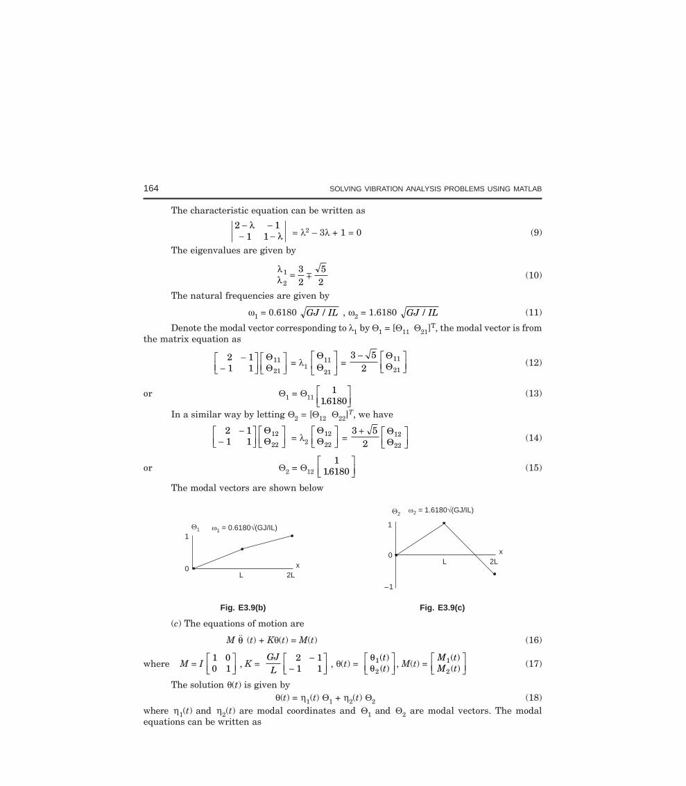
164 SOLVING VIBRATION ANALYSIS PROBLEMS USING MATLAB
The characteristic equation can be written as
2 11 1
− −− −
λλ = λ2 – 3λ + 1 = 0 (9)
The eigenvalues are given by
λλ
1
2
32
52
= (10)
The natural frequencies are given by
ω1 = 0.6180 GJ IL/ , ω2 = 1.6180 GJ IL/ (11)
Denote the modal vector corresponding to λ1 by Θ1 = [Θ11 Θ21]T, the modal vector is fromthe matrix equation as
2 11 1
11
21
−−
LNM
OQPLNM
OQP
ΘΘ = λ1
ΘΘ
11
21
LNM
OQP =
3 52
11
21
− LNM
OQP
ΘΘ (12)
or Θ1 = Θ11 1
16180.LNM
OQP
(13)
In a similar way by letting Θ2 = [Θ12 Θ22]T, we have
2 11 1
12
22
−−
LNM
OQPLNM
OQP
ΘΘ = λ2
ΘΘ
12
22
LNM
OQP =
3 52
12
22
+ LNM
OQP
ΘΘ (14)
or Θ2 = Θ12 1
16180.LNM
OQP (15)
The modal vectors are shown below
= 0.6180 (GJ/IL)11
1
0L 2L
x
2
1
0L 2L
x
–1
= 1.6180 (GJ/IL)2
Fig. E3.9(b) Fig. E3.9(c)
(c) The equations of motion are
M θ (t) + Kθ(t) = M(t) (16)
where M = I 1 00 1LNM
OQP , K =
GJL
2 11 1
−−
LNM
OQP , θ(t) =
θθ
1
2
( )( )tt
LNM
OQP , M(t) =
M tM t
1
2
( )( )
LNM
OQP (17)
The solution θ(t) is given byθ(t) = η1(t) Θ1 + η2(t) Θ2 (18)
where η1(t) and η2(t) are modal coordinates and Θ1 and Θ2 are modal vectors. The modalequations can be written as
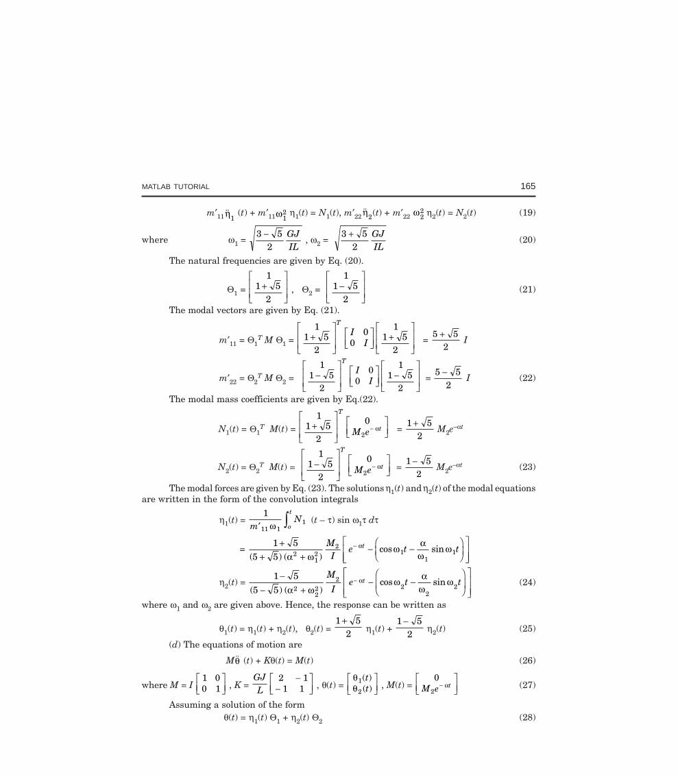
MATLAB TUTORIAL 165
m′11η1 (t) + m′11ω1
2 η1(t) = N1(t), m′22η2(t) + m′22 ω2
2 η2(t) = N2(t) (19)
where ω1 = 3 5
2− GJ
IL , ω2 =
3 52
+ GJIL
(20)
The natural frequencies are given by Eq. (20).
Θ1 = 1
1 52
+L
NMM
O
QPP , Θ2 =
11 5
2−
L
NMM
O
QPP (21)
The modal vectors are given by Eq. (21).
m′11 = Θ1T M Θ1 =
11 5
2
00
11 5
2+
L
NMM
O
QPP
LNM
OQP +L
NMM
O
QPP
T
II =
5 52
+ I
m′22 = Θ2T M Θ2 =
11 5
2
00
11 5
2−
L
NMM
O
QPP
LNM
OQP −L
NMM
O
QPP
T
II =
5 52
− I (22)
The modal mass coefficients are given by Eq.(22).
N1(t) = Θ1T M(t) =
11 5
2
02
+L
NMM
O
QPP
LNM
OQP−
T
tM e α = 1 5
2+
M2e–αt
N2(t) = Θ2T M(t) =
11 5
2
02
−L
NMM
O
QPP
LNM
OQP−
T
tM e α = 1 5
2−
M2e–αt (23)
The modal forces are given by Eq. (23). The solutions η1(t) and η2(t) of the modal equationsare written in the form of the convolution integrals
η1(t) = 1
11 11m
No
t
′ zω (t – τ) sin ω1τ dτ
= 1 5
5 5 212
21
11
++ +
− −FHG
IKJ
LNMM
OQPP
−
( ) ( )cos sin
α ωω α
ωωαM
Ie t tt
η2(t) = 1 5
5 5 222
22
22
−− +
− −FHG
IKJ
LNMM
OQPP
−
( ) ( )cos sin
α ωω α
ωωα
M
Ie t tt (24)
where ω1 and ω2 are given above. Hence, the response can be written as
θ1(t) = η1(t) + η2(t), θ2(t) = 1 5
2+
η1(t) + 1 5
2−
η2(t) (25)
(d) The equations of motion are
Mθ (t) + Kθ(t) = M(t) (26)
where M = I 1 00 1
LNM
OQP , K =
GJL
2 11 1
−−
LNM
OQP , θ(t) =
θθ
1
2
( )( )tt
LNM
OQP , M(t) =
02M e t−
LNM
OQPα (27)
Assuming a solution of the formθ(t) = η1(t) Θ1 + η2(t) Θ2 (28)
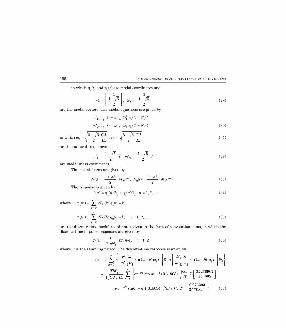
166 SOLVING VIBRATION ANALYSIS PROBLEMS USING MATLAB
in which η1(t) and η2(t) are modal coordinates and
Θ1 = 1
1 52
+L
NMM
O
QPP , Θ2 =
11 5
2−
L
NMM
O
QPP (29)
are the modal vectors. The modal equations are given by
m′11 η1 (t) + m′11 ω1
2 η1(t) = N1(t)
m′22η2 (t) + m′22 ω2
2 η2(t) = N2(t) (30)
in which ω1 = 3 5
2− GJ
IL , ω2 =
3 52
+ GJIL
(31)
are the natural frequencies.
m′11 = 1 5
2+
I, m′22 = 1 5
2−
I (32)
are modal mass coefficients.The modal forces are given by
N1(t) = 1 5
2+
M2e–αt, N2(t) =
1 52
− M2e
–αt (33)
The response is given byθ(n) = η1(n)Θ1 + η2(n)Θ2, n = 1, 2, … (34)
where η1(n) = k
n
N=
∑0
1 (k) g1(n – k),
η2(n) = k
n
N=∑
02 (k) g2(n – k), n = 1, 2, … (35)
are the discrete-time modal coordinates given in the form of convolution sums, in which thediscrete time impulse responses are given by
gi(n) = T
m ii i′ ω
sin nωiT, i = 1, 2 (36)
where T is the sampling period. The discrete-time response is given by
θ(n) = T k
n N k
mn k T
N k
mn k T
=∑ ′
−LNMM
OQPP
+′
−LNMM
OQPP
RS|T|
UV|W|0
1
11 11 1
2
22 22 2
( )sin ( )
( )sin ( )
ωω
ωωΘ Θ
= TM
GJ ILe n k
GJIL
Tk
nk2
010 618034
0 7236907117082/
sin ( ) ...
=
−∝∑ − LNM
OQP
RS|T|
T
+ e– αkT sin(n – k)1.618034 GJ IL/ T −L
NMOQPUVW
0 2763930 17082
.. (37)
MATLAB TUTORIAL 167
Denoting GJ IL/ = 1, M2/I = 1, α = 1 and T = 0.01 s, the response is given by
θ(n) = 0.01 k
nke n k
=
−∑ − LNM
OQP
RST0
0.01 0 618034 0 7236071170820
sin . ( ) ..
+ sin 1.618034(n – k)T −L
NMOQPUVW
0 2763930 170820
.. (38)
The discrete-time response sequence is given by
θ(0) = 00LNMOQP
θ(1) = 0.01 sin . ..0 00618034 0 723607
1170820LNM
OQP
RST + sin 0.0161803 −L
NMOQPUVW
0 2763931170820
..
= 182291 109 999 10
9
5..
××
LNM
OQP
−
−
θ(2) = 0.01 [sin ( . ) sin . ] ..0 00618034 2 0 00618034 0 723607
11708200.01× + L
NMOQP
RST−e
+ [sin(0.0161803 × 2) + e– 0.01 sin 0.0161803] −L
NMOQPUVW
0 2763930 170820
..
= 154497 102 990 10
8
4.
.×
×LNM
OQP
−
− (39)
(e) The response θi(n) (i = 1, 2) is plotted in Fig. E3.9 (d) obtained from the followingMATLAB program.
% Response of 2-degree of freedom system
clear
clf
I=1; % mass
k=1;%=GJ/L torsional stiffness
M=I*[1 0;0 1];% mass matrix
K=k*[2 -1;-1 1];%stiffness matrix
[u,W]=eig(K,M);% eigenvalue problem
% W= eigenvalues
u(:,1)=u(:,1)/max(u(:,1)); % normalization
u(:,2)=u(:,2)/max(u(:,2));
[w(1),I1]=min(max(W)); % relabeling of the eigenvalues
[w(2),I2]=max(max(W));
w(1)=sqrt(w(1)); % Lowest natural frequency
w(2)=sqrt(w(2)); % highest natural frequency
U(:,1)=u(:,I1); % relabelling of the eigenvectors
U(:,2)=u(:,I2);
m1=U(:,1)'*M*U(:,1); % mass quantities
m2=U(:,2)'*M*U(:,2);
T=0.01; % sampling period
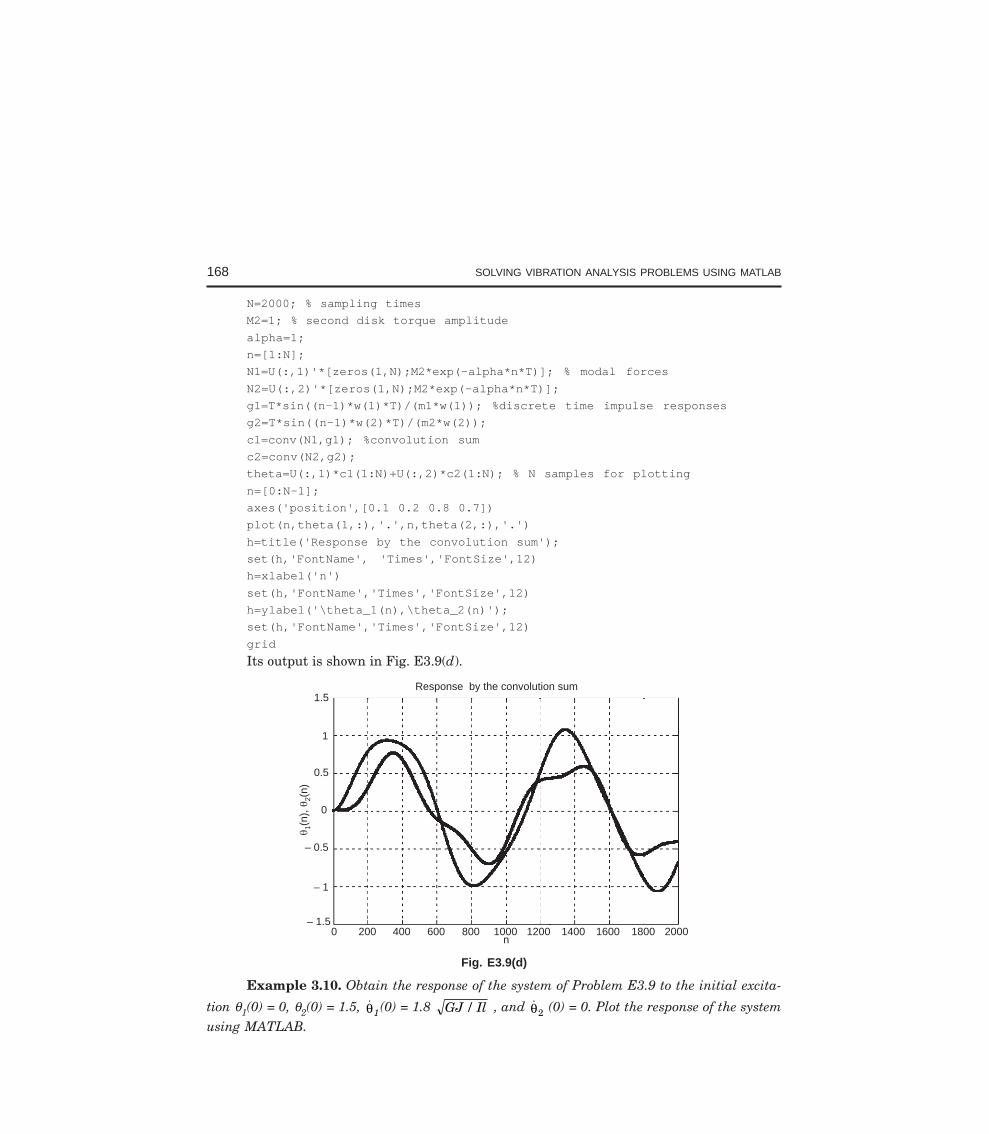
168 SOLVING VIBRATION ANALYSIS PROBLEMS USING MATLAB
N=2000; % sampling times
M2=1; % second disk torque amplitude
alpha=1;
n=[1:N];
N1=U(:,1)'*[zeros(1,N);M2*exp(-alpha*n*T)]; % modal forces
N2=U(:,2)'*[zeros(1,N);M2*exp(-alpha*n*T)];
g1=T*sin((n-1)*w(1)*T)/(m1*w(1)); %discrete time impulse responses
g2=T*sin((n-1)*w(2)*T)/(m2*w(2));
c1=conv(N1,g1); %convolution sum
c2=conv(N2,g2);
theta=U(:,1)*c1(1:N)+U(:,2)*c2(1:N); % N samples for plotting
n=[0:N-1];
axes('position',[0.1 0.2 0.8 0.7])
plot(n,theta(1,:),'.',n,theta(2,:),'.')
h=title('Response by the convolution sum');
set(h,'FontName', 'Times','FontSize',12)
h=xlabel('n')
set(h,'FontName','Times','FontSize',12)
h=ylabel('\theta_1(n),\theta_2(n)');
set(h,'FontName','Times','FontSize',12)
grid
Its output is shown in Fig. E3.9(d).
Response by the convolution sum1.5
1
– 0.5
0.5
0
– 1
– 1.5
12
(n),
(n)
0 200 400 600 800 1000 1200 1400 1600 1800 2000n
Fig. E3.9(d)
Example 3.10. Obtain the response of the system of Problem E3.9 to the initial excita-
tion θ1(0) = 0, θ2(0) = 1.5, θ1(0) = 1.8 GJ Il/ , and θ2 (0) = 0. Plot the response of the systemusing MATLAB.
MATLAB TUTORIAL 169
Solution:The initial conditions are given as
θ1(0) = 0, θ2(0) = 1.5, θ1 (0) = 1.8
GJIL
, θ2(0) = 0 (1)
From Problem V3.9, we have
ω1 = 0.6180 GJIL
, Θ1 = ΘΘ
11
21
LNM
OQP = Θ11
11 6180.
LNM
OQP
ω2 = 1.6180 GJIL
, Θ2 = ΘΘ
12
22
LNM
OQP = Θ12
11 6180.
LNM
OQP (2)
The response to the initial excitation is a superposition of the natural modes. Henceθ(t) = C1 cos(ω1t – φ1)Θ1 + C2 cos(ω2t – φ2)Θ2
or θ(t) = C1 (cos ω1t cos φ1 + sin ω1t sin φ1)Θ1+ C2 (cos ω2t cos φ2 + sin ω2t sin φ2)Θ2 (3)
and θ (t) = C1ω1(sin ω1t cos φ1 – cos ω1t sin φ1)Θ1– C2ω2 (sin ω2t cos φ2 – cos ω2t sin φ2)Θ2
If t = 0, then Eq. (3) becomes
θ(0) = θθ
1
2
00
( )( )
LNM
OQP = C1 cos φ1
ΘΘ
11
21
LNM
OQP + C2 cos φ2
ΘΘ
12
22
LNM
OQP
θ (0) = ( ) ( )θθ
1
2
00
LNMM
OQPP = C1ω1 sin φ1
ΘΘ
11
21
LNM
OQP + C2ω2 sin φ2
ΘΘ
12
22
LNM
OQP (4)
From Eq. (4) we have,
C1 cos φ1 = Θ Θ
Θ22 10 12 20θ θ−
| | , C2 cos φ2 =
Θ ΘΘ
11 20 21 10θ θ−| |
C1 sin φ1 = Θ Θ
Θ22 10 12 20
1
| |
θ θω
− , C2 sin φ2 =
Θ ΘΘ
11 20 21 10
2
| |
θ θω
−(5)
where θ10 = θ1(0), θ20 = θ2(0), θ 10 = θ 1(0), θ 20 = θ 2(0) and |Θ| is the determinant of the matrix
Θ = Θ ΘΘ Θ
11 12
21 22
LNM
OQP (6)
Letting Θ11 = Θ12 = 1,
C1 cos φ1 = 1 5.| |Θ , C2 cos φ2 =
1 5.| |Θ ,
C1 sin φ1 = 1 8.| |Θ , C2 sin φ2 =
1 8.| |Θ
|Θ| = 1 1
16180 16180. .− = – 2.2360 (7)
170 SOLVING VIBRATION ANALYSIS PROBLEMS USING MATLAB
The response to the given initial excitation is given by
θ(t) = θθ
1
2
( )( )tt
LNM
OQP =
12 2360
1 5 1 8 11 61801 1.
( . cos . cos ) .ω ωt t+ LNM
OQP
LNM
+ (– 1.5 cos ω2t + 1.8 sin ω2t) 1
0 6180−LNM
OQPOQP.
or by components
θ1(t) = 0.6708 cos . cos .0 6180 1 6180GJIL
tGJIL
t−FHG
IKJ
+ 0.8060 sin . sin .0 6180 1 6180GJIL
tGJIL
t+FHG
IKJ
θ2(t) = 1.0854 cos 0.6180 GJIL
t + 1.3025 sin 0.6180 GJIL
t
+ 0.4146 cos 1.6180 GJIL
t – 0.4975 sin 106180 GJIL
t (8)
The MATLAB program listed as follows:% response of a two-degree-of freedom system to initial excitations
clear
clf
I=1; % inertia
k=1;%=GJ/L stiffness
M=I*[1 0;0 1];% mass
K=k*[2 -1;-1 1];%stiffness
[u,W]=eig(K,M);% eigenvalue problem
% W=matrix of eigenvalues
u(:,1)=u(:,1)/max(u(:,1)); % normalization
u(:,2)=u(:,2)/max(u(:,2));
[w(1),I1]=min(max(W)); % relabeling
[w(2),I2]=max(max(W));
w(1)=sqrt(w(1)); % lowest natural frequency
w(2)=sqrt(w(2)); % highest natural frequency
U(:,1)=u(:,I1); % relabelling
U(:,2)=u(:,I2);
x0=[0;2];% Initial displacement
v0=[2*sqrt(k/I);0]; % initial velocity
t=[0:0.1:20]; % initial time, time increment, final time
% displacement
x1=(((U(2,2)*x0(1)-U(1,2)*x0(2))*cos(w(1)*t)+(U(2,2)*v0(1)-
U(1,2)*v0(2))*sin(w(1)*t)/w(1))*U(1,1)+((U(1,1)*x0(2)
-U(2,1)*x0(1))*cos(w(2)*t)+(U(1,1)*v0(2)-U(2,1)*v0(1))*sin(w(2)*t)
/w(2))*U(1,2))/det(U);
x2=(((U(2,2)*x0(1)-U(1,2)*x0(2))*cos(w(1)*t)+(U(2,2)*v0(1)-
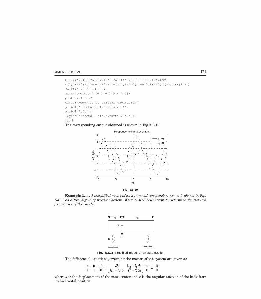
MATLAB TUTORIAL 171
U(1,2)*v0(2))*sin(w(1)*t)/w(1))*U(2,1)+((U(1,1)*x0(2)-
U(2,1)*x0(1))*cos(w(2)*t)+(U(1,1)*v0(2)-U(2,1)*v0(1))*sin(w(2)*t)
/w(2))*U(2,2))/det(U);
axes('position',[0.2 0.3 0.6 0.5])
plot(t,x1,t,x2)
title('Response to initial excitation')
ylabel('\theta_1(t),\theta_2(t)')
xlabel('t[s]')
legend('\theta_1(t)','\theta_2(t)',1)
grid
The corresponding output obtained is shown in Fig.E 3.10
Response to initial excitation3
2
1
0
– 1
– 2
– 3
12
(t),
(t)
0 5 10 15 20t[s]
1 (t)
2 (t)
Fig. E3.10
Example 3.11. A simplified model of an automobile suspension system is shown in Fig.E3.11 as a two degree of freedom system. Write a MATLAB script to determine the naturalfrequencies of this model.
G
k kx
l1 l2
Fig. E3.11 Simplified model of an automobile.
The differential equations governing the motion of the system are given as
m x k l l kl l k l l k
x00 1
2 00
2 1
2 1 22
12
LNM
OQPLNM
OQP +
−− −
LNM
OQPLNM
OQP = L
NMOQP
( )( ) ( )θ θ
where x is the displacement of the mass center and θ is the angular rotation of the body fromits horizontal position.
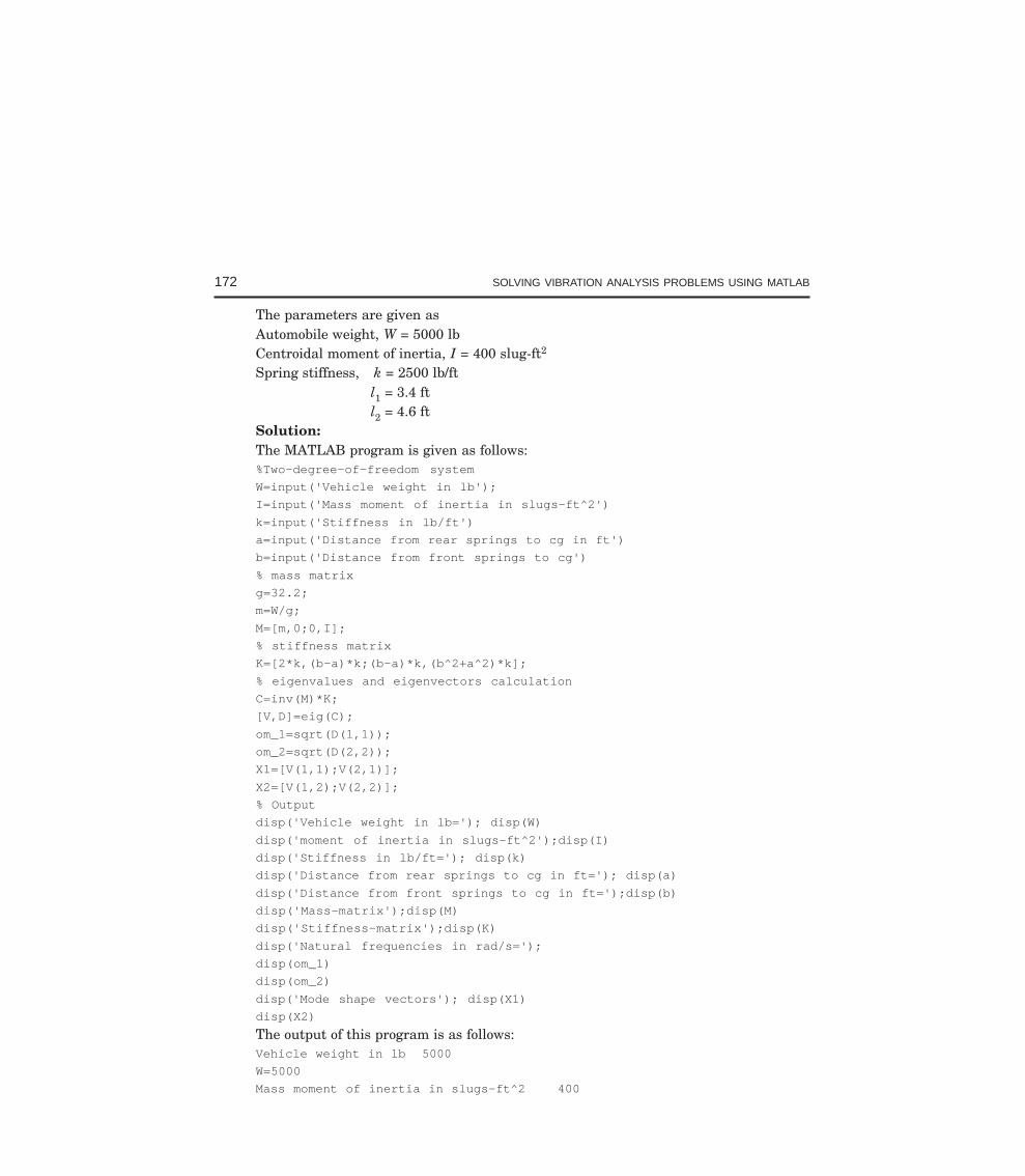
172 SOLVING VIBRATION ANALYSIS PROBLEMS USING MATLAB
The parameters are given asAutomobile weight, W = 5000 lbCentroidal moment of inertia, I = 400 slug-ft2
Spring stiffness, k = 2500 lb/ftl1 = 3.4 ftl2 = 4.6 ft
Solution:The MATLAB program is given as follows:%Two-degree-of-freedom system
W=input('Vehicle weight in lb');
I=input('Mass moment of inertia in slugs-ft^2')
k=input('Stiffness in lb/ft')
a=input('Distance from rear springs to cg in ft')
b=input('Distance from front springs to cg')
% mass matrix
g=32.2;
m=W/g;
M=[m,0;0,I];
% stiffness matrix
K=[2*k,(b-a)*k;(b-a)*k,(b^2+a^2)*k];
% eigenvalues and eigenvectors calculation
C=inv(M)*K;
[V,D]=eig(C);
om_1=sqrt(D(1,1));
om_2=sqrt(D(2,2));
X1=[V(1,1);V(2,1)];
X2=[V(1,2);V(2,2)];
% Output
disp('Vehicle weight in lb='); disp(W)
disp('moment of inertia in slugs-ft^2');disp(I)
disp('Stiffness in lb/ft='); disp(k)
disp('Distance from rear springs to cg in ft='); disp(a)
disp('Distance from front springs to cg in ft=');disp(b)
disp('Mass-matrix');disp(M)
disp('Stiffness-matrix');disp(K)
disp('Natural frequencies in rad/s=');
disp(om_1)
disp(om_2)
disp('Mode shape vectors'); disp(X1)
disp(X2)
The output of this program is as follows:Vehicle weight in lb 5000
W=5000
Mass moment of inertia in slugs-ft^2 400
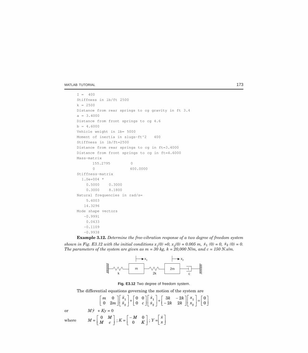
MATLAB TUTORIAL 173
I = 400
Stiffness in lb/ft 2500
k = 2500
Distance from rear springs to cg gravity in ft 3.4
a = 3.4000
Distance from front springs to cg 4.6
b = 4.6000
Vehicle weight in lb= 5000
Moment of inertia in slugs-ft^2 400
Stiffness in lb/ft=2500
Distance from rear springs to cg in ft=3.4000
Distance from front springs to cg in ft=4.6000
Mass-matrix
155.2795 0
0 400.0000
Stiffness-matrix
1.0e+004 *
0.5000 0.3000
0.3000 8.1800
Natural frequencies in rad/s=
5.6003
14.3296
Mode shape vectors
-0.9991
0.0433
-0.1109
-0.9938
Example 3.12. Determine the free-vibration response of a two degree of freedom system
shown in Fig. E3.12 with the initial conditions x1(0) =0, x2(0) = 0.005 m, x1 (0) = 0, x2 (0) = 0.The parameters of the system are given as m = 30 kg, k = 20,000 N/m, and c = 150 N.s/m.
x1
m2k c
2mk
x2
Fig. E3.12 Two degree of freedom system.
The differential equations governing the motion of the system are
mm
xx c
xx
k kk k
xx
00 2
0 00
3 22 2
00
1
2
1
2
1
2
LNM
OQPLNM
OQP
+ LNM
OQPLNM
OQP
+ −−
LNM
OQPLNM
OQP
= LNM
OQP
or M y + Ky = 0
where M = 0 MM c
LNM
OQP ; K =
−LNM
OQP
MK0
0 ; Y =xx
LNM
OQP
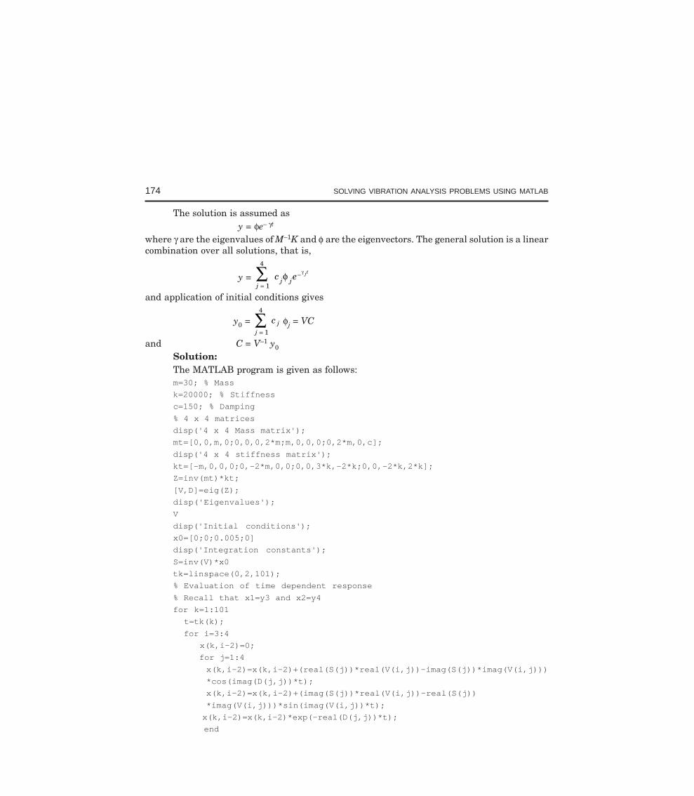
174 SOLVING VIBRATION ANALYSIS PROBLEMS USING MATLAB
The solution is assumed asy = φe– γt
where γ are the eigenvalues of M–1K and φ are the eigenvectors. The general solution is a linearcombination over all solutions, that is,
y = j =∑
1
4
c ej jjtφ γ−
and application of initial conditions gives
y0 = j
jc=
∑1
4
φj = VC
and C = V–1 y0Solution:The MATLAB program is given as follows:m=30; % Mass
k=20000; % Stiffness
c=150; % Damping
% 4 x 4 matrices
disp('4 x 4 Mass matrix');
mt=[0,0,m,0;0,0,0,2*m;m,0,0,0;0,2*m,0,c];
disp('4 x 4 stiffness matrix');
kt=[-m,0,0,0;0,-2*m,0,0;0,0,3*k,-2*k;0,0,-2*k,2*k];
Z=inv(mt)*kt;
[V,D]=eig(Z);
disp('Eigenvalues');
V
disp('Initial conditions');
x0=[0;0;0.005;0]
disp('Integration constants');
S=inv(V)*x0
tk=linspace(0,2,101);
% Evaluation of time dependent response
% Recall that x1=y3 and x2=y4
for k=1:101
t=tk(k);
for i=3:4
x(k,i-2)=0;
for j=1:4
x(k,i-2)=x(k,i-2)+(real(S(j))*real(V(i,j))-imag(S(j))*imag(V(i,j)))
*cos(imag(D(j,j))*t);
x(k,i-2)=x(k,i-2)+(imag(S(j))*real(V(i,j))-real(S(j))
*imag(V(i,j)))*sin(imag(V(i,j))*t);
x(k,i-2)=x(k,i-2)*exp(-real(D(j,j))*t);
end
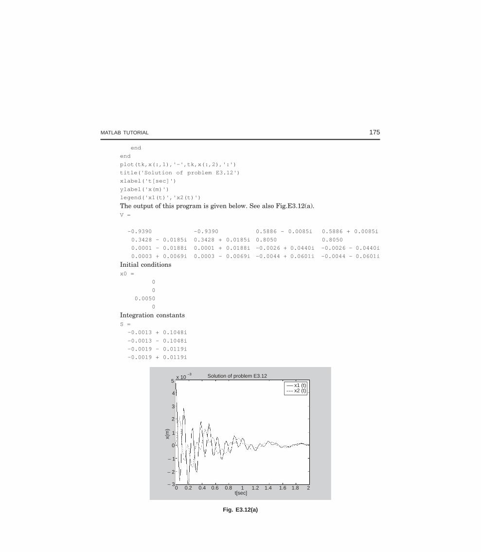
MATLAB TUTORIAL 175
end
end
plot(tk,x(:,1),'-',tk,x(:,2),':')
title('Solution of problem E3.12')
xlabel('t[sec]')
ylabel('x(m)')
legend('x1(t)','x2(t)')
The output of this program is given below. See also Fig.E3.12(a).V =
-0.9390 -0.9390 0.5886 - 0.0085i 0.5886 + 0.0085i
0.3428 - 0.0185i 0.3428 + 0.0185i 0.8050 0.8050
0.0001 - 0.0188i 0.0001 + 0.0188i -0.0026 + 0.0440i -0.0026 - 0.0440i
0.0003 + 0.0069i 0.0003 - 0.0069i -0.0044 + 0.0601i -0.0044 - 0.0601i
Initial conditionsx0 =
0
0
0.0050
0
Integration constantsS =
-0.0013 + 0.1048i
-0.0013 - 0.1048i
-0.0019 - 0.0119i
-0.0019 + 0.0119i
Solution of problem E3.125
4
3
2
1
0
– 1
– 2
– 3
x 10–3
0 0.2 0.4 0.6 0.8 1 1.2 1.4 1.6 1.8 2
x1 (t)x2 (t)
x(m
)
t[sec]
Fig. E3.12(a)
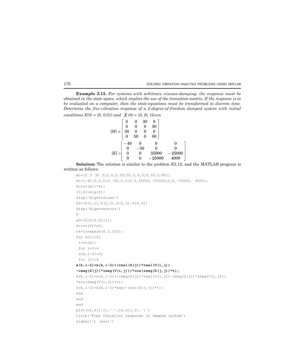
176 SOLVING VIBRATION ANALYSIS PROBLEMS USING MATLAB
Example 3.13. For systems with arbitrary viscous-damping, the response must beobtained in the state-space, which implies the use of the transition-matrix. If the response is tobe evaluated on a computer, then the state-equations must be transformed to discrete time.Determine the free-vibration response of a 2-degree-of-freedom damped system with initial
conditions X(0) = 0, 0.01 and X (0) = 0, 0. Given
[M] =
0 0 30 00 0 0 5030 0 0 00 50 0 80
L
N
MMM
O
Q
PPP
[K] =
−−
−−
L
N
MMM
O
Q
PPP
40 0 0 00 50 0 00 0 35000 250000 0 25000 4000
Solution: The solution is similar to the problem E3.12, and the MATLAB program iswritten as follows:
mt=[0 0 30 0;0,0,0,50;30,0,0,0;0,50,0,80];
kt=[-40,0,0,0;0,-50,0,0;0,0,35000,-25000;0,0,-25000, 4000];
Z=inv(mt)*kt;
[V,D]=eig(Z);
disp('Eigenvalues')
DS=[D(1,1),D(2,2),D(3,3),D(4,4)]
disp('Eigenvectors')
V
x0=[0;0;0.01;0];
S=inv(V)*x0;
tk=linspace(0,2,101);
for k=1:101
t=tk(k);
for i=3:4
x(k,i-2)=0;
for j=1:4
x(k,i-2)=x(k,i-2)+(real(S(j))*real(V(i,j))
-imag(S(j))*imag(V(i,j)))*cos(imag(D(j,j))*t);
x(k,i-2)=x(k,i-2)+(imag(S(j))*real(V(i,j))-imag(S(j))*imag(V(i,j)))
*sin(imag(V(i,j))*t);
x(k,i-2)=x(k,i-2)*exp(-real(D(j,j))*t);
end
end
end
plot(tk,x(:,1),'-',tk,x(:,2),':')
title('Free Vibration response of damped system')
xlabel('t (sec)')
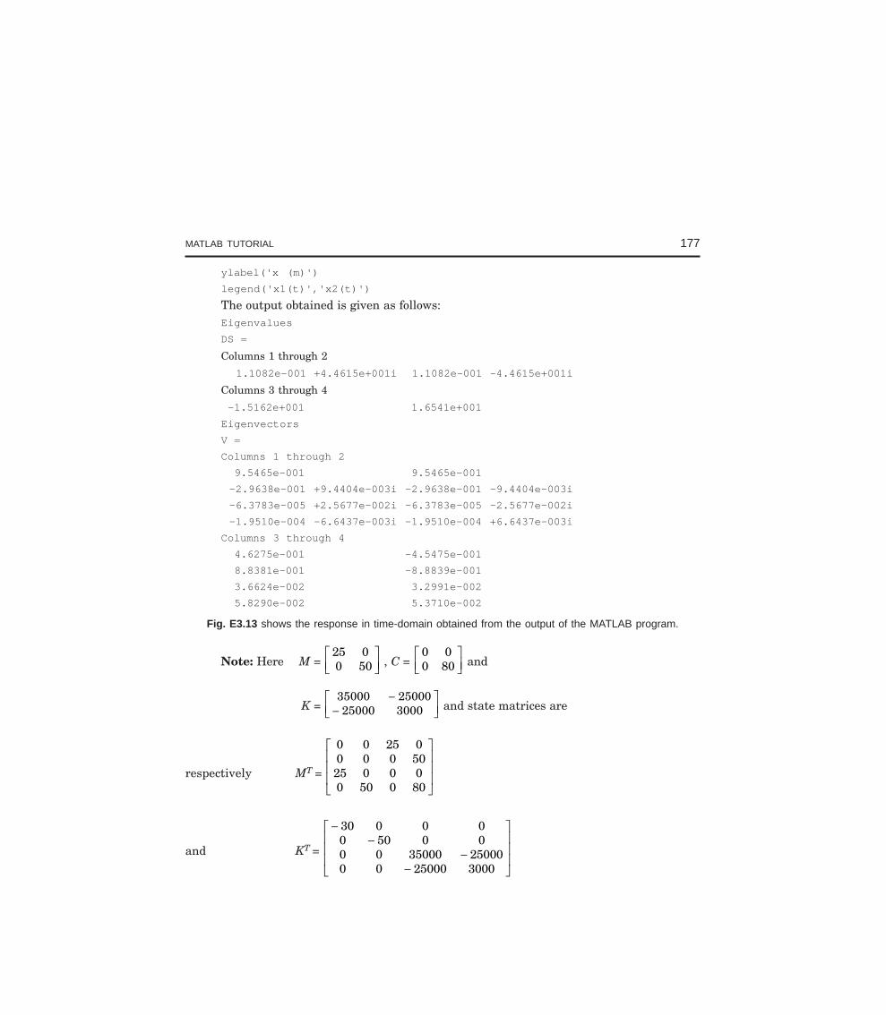
MATLAB TUTORIAL 177
ylabel('x (m)')
legend('x1(t)','x2(t)')
The output obtained is given as follows:Eigenvalues
DS =
Columns 1 through 2
1.1082e-001 +4.4615e+001i 1.1082e-001 -4.4615e+001i
Columns 3 through 4
-1.5162e+001 1.6541e+001
Eigenvectors
V =
Columns 1 through 2
9.5465e-001 9.5465e-001
-2.9638e-001 +9.4404e-003i -2.9638e-001 -9.4404e-003i
-6.3783e-005 +2.5677e-002i -6.3783e-005 -2.5677e-002i
-1.9510e-004 -6.6437e-003i -1.9510e-004 +6.6437e-003i
Columns 3 through 4
4.6275e-001 -4.5475e-001
8.8381e-001 -8.8839e-001
3.6624e-002 3.2991e-002
5.8290e-002 5.3710e-002
Fig. E3.13 shows the response in time-domain obtained from the output of the MATLAB program.
Note: Here M = 25 00 50
LNM
OQP , C =
0 00 80
LNM
OQP and
K = 35000 2500025000 3000
−−
LNM
OQP and state matrices are
respectively MT =
0 0 25 00 0 0 5025 0 0 00 50 0 80
L
N
MMM
O
Q
PPP
and KT =
−−
−−
L
N
MMM
O
Q
PPP
30 0 0 00 50 0 00 0 35000 250000 0 25000 3000
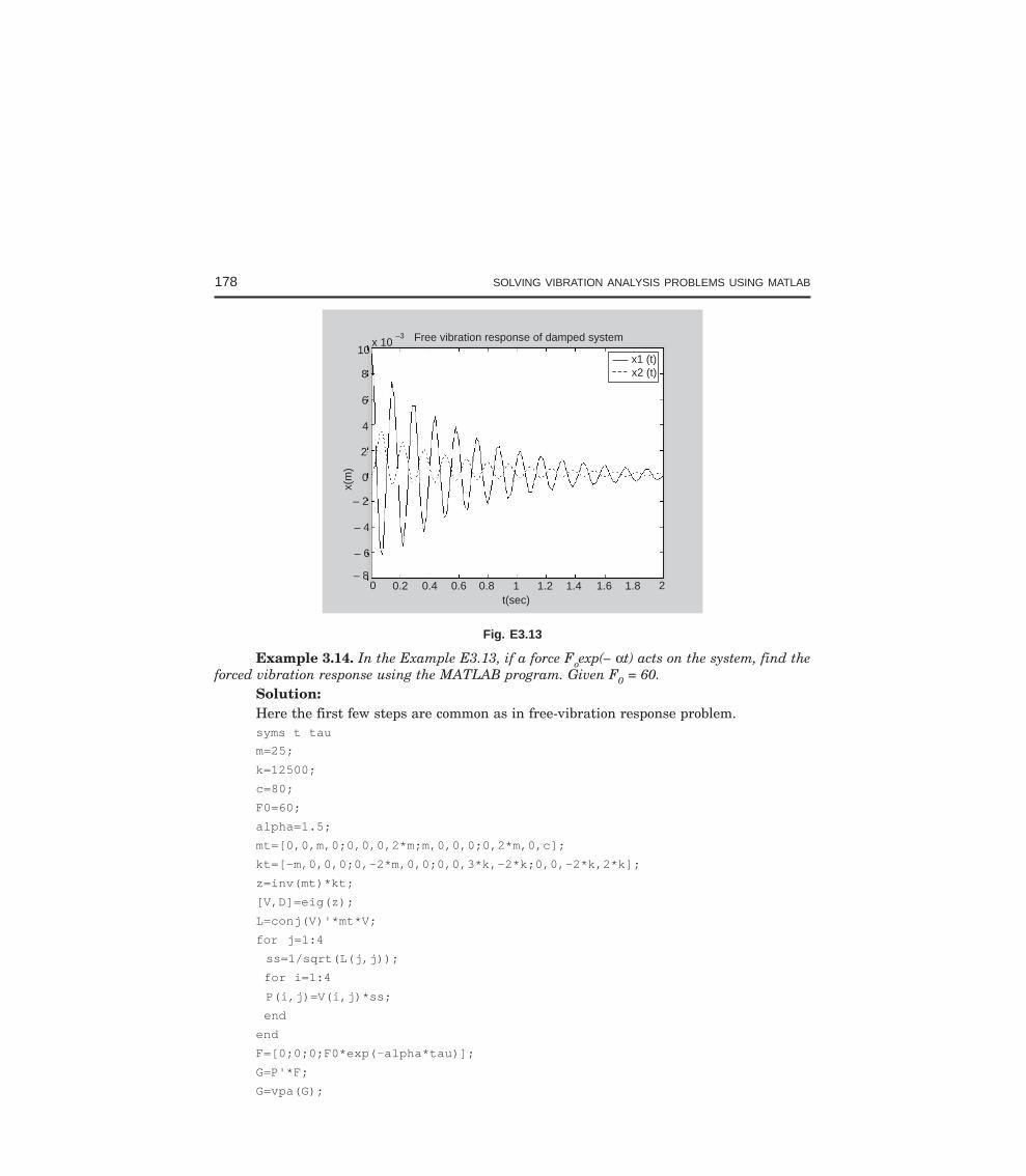
178 SOLVING VIBRATION ANALYSIS PROBLEMS USING MATLAB
Free vibration response of damped systemx 10–3
10
8
6
4
2
0
– 2
– 4
– 6
– 80 0.2 0.4 0.6 0.8 1 1.2 1.4 1.6 1.8 2
x1 (t)x2 (t)
t(sec)
x(m
)
Fig. E3.13
Example 3.14. In the Example E3.13, if a force Foexp(– αt) acts on the system, find theforced vibration response using the MATLAB program. Given F0 = 60.
Solution:Here the first few steps are common as in free-vibration response problem.syms t tau
m=25;
k=12500;
c=80;
F0=60;
alpha=1.5;
mt=[0,0,m,0;0,0,0,2*m;m,0,0,0;0,2*m,0,c];
kt=[-m,0,0,0;0,-2*m,0,0;0,0,3*k,-2*k;0,0,-2*k,2*k];
z=inv(mt)*kt;
[V,D]=eig(z);
L=conj(V)'*mt*V;
for j=1:4
ss=1/sqrt(L(j,j));
for i=1:4
P(i,j)=V(i,j)*ss;
end
end
F=[0;0;0;F0*exp(-alpha*tau)];
G=P'*F;
G=vpa(G);
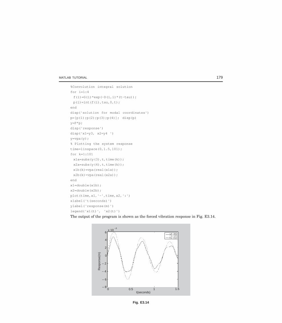
MATLAB TUTORIAL 179
%Convolution integral solution
for i=1:4
f(i)=G(i)*exp(-D(i,i)*(t-tau));
p(i)=int(f(i),tau,0,t);
end
disp('solution for modal coordinates')
p=[p(1);p(2);p(3);p(4)]; disp(p)
y=P*p;
disp('response')
disp('x1=y3, x2=y4 ')
y=vpa(y);
% Plotting the system response
time=linspace(0,1.5,101);
for k=1:101
x1a=subs(y(3),t,time(k));
x2a=subs(y(4),t,time(k));
x1b(k)=vpa(real(x1a));
x2b(k)=vpa(real(x2a));
end
x1=double(x1b);
x2=double(x2b);
plot(time,x1,'-',time,x2,':')
xlabel('t(seconds)')
ylabel('response(m)')
legend('x1(t)', 'x2(t)')
The output of the program is shown as the forced vibration response in Fig. E3.14.
t(seconds)
Res
pons
e(m
)
6
4
2
0
– 2
– 4
– 6
x 10–3
– 80 0.5 1 1.5
x1 (t)x2 (t)
Fig. E3.14
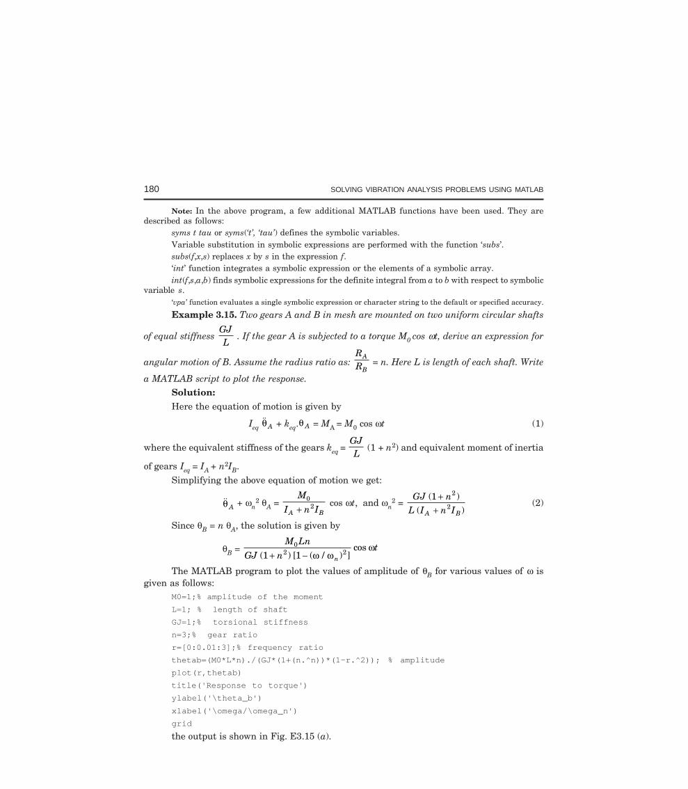
180 SOLVING VIBRATION ANALYSIS PROBLEMS USING MATLAB
Note: In the above program, a few additional MATLAB functions have been used. They aredescribed as follows:
syms t tau or syms(‘t’, ‘tau’) defines the symbolic variables.Variable substitution in symbolic expressions are performed with the function ‘subs’.subs(f,x,s) replaces x by s in the expression f.‘int’ function integrates a symbolic expression or the elements of a symbolic array.int(f,s,a,b) finds symbolic expressions for the definite integral from a to b with respect to symbolic
variable s.‘vpa’ function evaluates a single symbolic expression or character string to the default or specified accuracy.
Example 3.15. Two gears A and B in mesh are mounted on two uniform circular shafts
of equal stiffness GJL
. If the gear A is subjected to a torque M0 cos ωt, derive an expression for
angular motion of B. Assume the radius ratio as: RR
A
B = n. Here L is length of each shaft. Write
a MATLAB script to plot the response.Solution:Here the equation of motion is given by
Ieq θ A + keq.θ A = MA = M0 cos ωt (1)
where the equivalent stiffness of the gears keq = GJL
(1 + n2) and equivalent moment of inertia
of gears Ieq = IA + n2IB.Simplifying the above equation of motion we get:
θ A + ωn2 θA =
M
I n IA B
02+
cos ωt, and ωn2 =
GJ n
L I n IA B
( )( )
1 2
2+
+(2)
Since θB = n θA, the solution is given by
θB = M Ln
GJ nt
n
02 21 1( ) [ ( / ) ]
cos+ − ω ω
ω
The MATLAB program to plot the values of amplitude of θB for various values of ω isgiven as follows:
M0=1;% amplitude of the moment
L=1; % length of shaft
GJ=1;% torsional stiffness
n=3;% gear ratio
r=[0:0.01:3];% frequency ratio
thetab=(M0*L*n)./(GJ*(1+(n.^n))*(1-r.^2)); % amplitude
plot(r,thetab)
title('Response to torque')
ylabel('\theta_b')
xlabel('\omega/\omega_n')
grid
the output is shown in Fig. E3.15 (a).
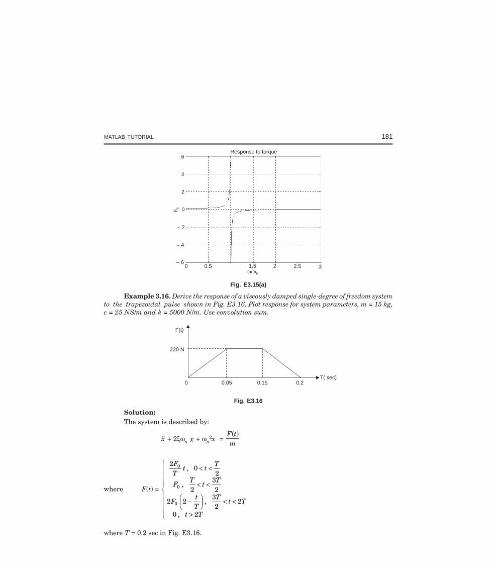
MATLAB TUTORIAL 181
Response to torque6
4
2
0
– 2
– 4
– 60 0.5 1.5 2 2.5 3
/ n
b
Fig. E3.15(a)
Example 3.16. Derive the response of a viscously damped single-degree of freedom systemto the trapezoidal pulse shown in Fig. E3.16. Plot response for system parameters, m = 15 kg,c = 25 NS/m and k = 5000 N/m. Use convolution sum.
220 N
0.15
F(t)
T( sec)0.05 0.20
Fig. E3.16
Solution:The system is described by:
x + 2ξωn x + ωn2x =
F tm( )
where F(t) =
20
2
232
2 232
2
0 2
0
0
0
FT
t tT
FT
tT
FtT
Tt T
t T
,
,
,
,
< <
< <
−FHG
IKJ < <
>
R
S
||||
T
||||
where T = 0.2 sec in Fig. E3.16.
182 SOLVING VIBRATION ANALYSIS PROBLEMS USING MATLAB
The discrete time response by convolution sum is:
x(n) = k
n
F k g n k=
∑ −0
( ) ( )
The MATLAB script for this problem is given below:m=15; % mass
c=25; % damping
k=5000; % stiffness
F0=220;
T=0.2;
wn=sqrt(k/m); % Natural frequency
zeta=c/(2*sqrt(m*k));
Ts=0.003; % Sampling period
N=201; % sampling times
wd=wn*sqrt(1-zeta^2); % frequency
% force
for n=1:N,
if n<=(T/2)/Ts+1;F(n)=2*F0*(n-1)*Ts/T; else;F(n)=F0;end
if n>(3*T/2)/Ts+1;F(n)=2*F0*(2-(n-1)*Ts/T);end
if n>2*T/Ts+1;F(n)=0;end
end
n=[1:N];
g=Ts*exp(-(n-1)*zeta*wn*Ts).*sin((n-1)*wd*Ts)/(m*wd);
% discrete-time impulse response
c0=conv(F,g); % Convolution sum
c=c0(1:N); % plot to N samples
n=[0:N-1];
axes('position',[0.1 0.2 0.8 0.7])
plot(n,c,'.');
title('Response to the Trapezodial pulse');
xlabel('n')
ylabel('x(n) [m]')
grid
Output of this program is the Fig. E3.16(a)
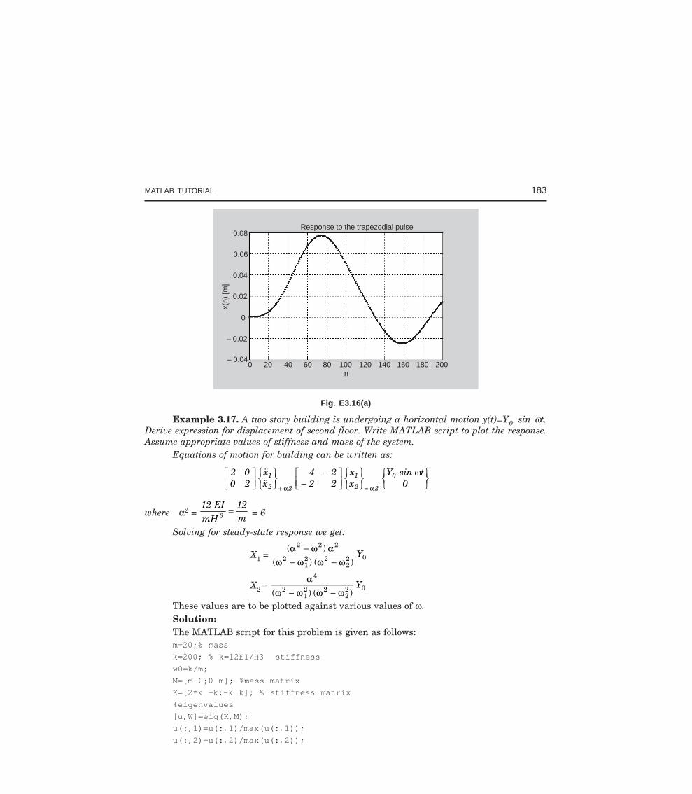
MATLAB TUTORIAL 183
Response to the trapezodial pulse0.08
0.06
0.04
0.02
0
– 0.02
– 0.04
x(n)
[m]
0 20 40 60 80 100 120 140 160 180 200n
Fig. E3.16(a)
Example 3.17. A two story building is undergoing a horizontal motion y(t)=Y0. sin ωt.Derive expression for displacement of second floor. Write MATLAB script to plot the response.Assume appropriate values of stiffness and mass of the system.
Equations of motion for building can be written as:
2 00 2
xx
4 22 2
xx
Y sin t0
1
2 2
1
2 2
0LNM
OQPRST
UVW−
−LNM
OQPRST
UVWRST
UVW+ =
α α
ω
where α2 = 12 EImH
12m3 = = 6
Solving for steady-state response we get:
X1 = ( )
( ) ( )α ω α
ω ω ω ω
2 2 2
212 2
22 0
−− −
Y
X2 = α
ω ω ω ω
4
212 2
22 0
( ) ( )− −Y
These values are to be plotted against various values of ω.Solution:The MATLAB script for this problem is given as follows:m=20;% mass
k=200; % k=12EI/H3 stiffness
w0=k/m;
M=[m 0;0 m]; %mass matrix
K=[2*k -k;-k k]; % stiffness matrix
%eigenvalues
[u,W]=eig(K,M);
u(:,1)=u(:,1)/max(u(:,1));
u(:,2)=u(:,2)/max(u(:,2));
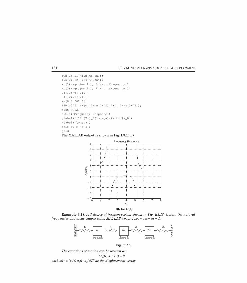
184 SOLVING VIBRATION ANALYSIS PROBLEMS USING MATLAB
[wn(1),I1]=min(max(W));
[wn(2),I2]=max(max(W));
wn(1)=sqrt(wn(1)); % Nat. frequency 1
wn(2)=sqrt(wn(2)); % Nat. frequency 2
U(:,1)=u(:,I1);
U(:,2)=u(:,I2);
w=[0:0.002:6];
T2=(w0^2)./((w.^2-wn(1)^2).*(w.^2-wn(2)^2));
plot(w,T2)
title('Frequency Response')
ylabel('\itX_2(\omega)/\itY_0')
xlabel('\omega')
axis([0 8 -5 5])
grid
The MATLAB output is shown in Fig. E3.17(a).
Frequency Response5
4
3
2
1
0
– 1
– 2
– 3
– 4
– 50 1 2 3 4 5 6 7 8
X(
)/y
20
Fig. E3.17(a)
Example 3.18. A 3-degree of freedom system shown in Fig. E3.18. Obtain the naturalfrequencies and mode shapes using MATLAB script. Assume k = m = 1.
m 2mkk 2k
2m2k
Fig. E3.18
The equations of motion can be written as:
M x(t) + Kx(t) = 0with x(t) = [x1(t) x2(t) x3(t)]T as the displacement vector
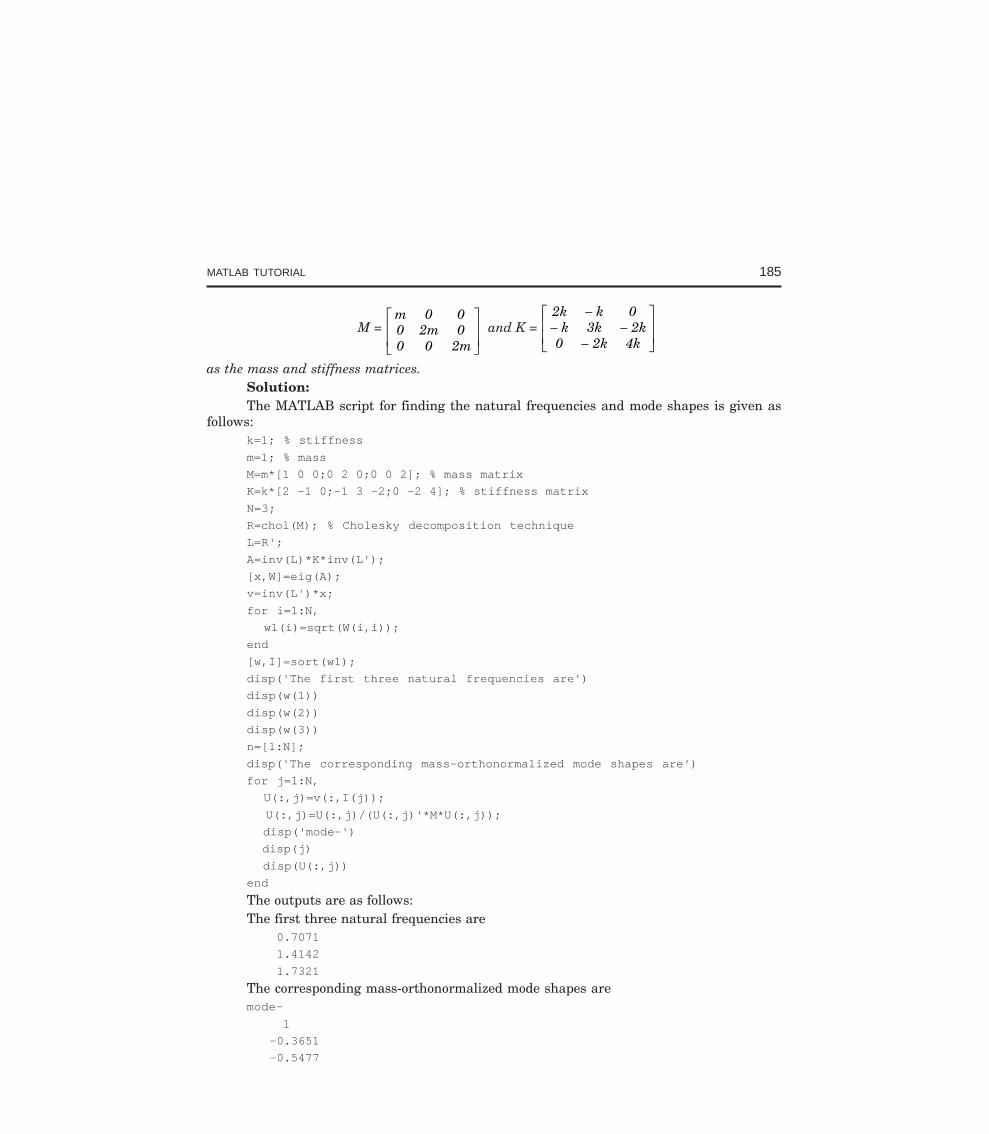
MATLAB TUTORIAL 185
M = m 0 00 2m 00 0 2m
L
NMM
O
QPP and K =
2k k 0k 3k 2k
0 2k 4k
−− −
−
L
NMM
O
QPP
as the mass and stiffness matrices.Solution:The MATLAB script for finding the natural frequencies and mode shapes is given as
follows:k=1; % stiffness
m=1; % mass
M=m*[1 0 0;0 2 0;0 0 2]; % mass matrix
K=k*[2 -1 0;-1 3 -2;0 -2 4]; % stiffness matrix
N=3;
R=chol(M); % Cholesky decomposition technique
L=R';
A=inv(L)*K*inv(L');
[x,W]=eig(A);
v=inv(L')*x;
for i=1:N,
w1(i)=sqrt(W(i,i));
end
[w,I]=sort(w1);
disp('The first three natural frequencies are')
disp(w(1))
disp(w(2))
disp(w(3))
n=[1:N];
disp('The corresponding mass-orthonormalized mode shapes are')
for j=1:N,
U(:,j)=v(:,I(j));
U(:,j)=U(:,j)/(U(:,j)'*M*U(:,j));
disp('mode-')
disp(j)
disp(U(:,j))
end
The outputs are as follows:The first three natural frequencies are 0.7071
1.4142
1.7321
The corresponding mass-orthonormalized mode shapes aremode-
1
-0.3651
-0.5477
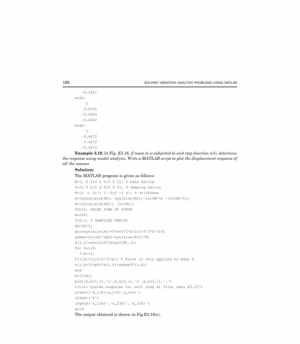
186 SOLVING VIBRATION ANALYSIS PROBLEMS USING MATLAB
-0.3651
mode-
2
0.8165
-0.0000
-0.4082
mode-
3
-0.4472
0.4472
-0.4472
Example 3.19. In Fig. E3.18, if mass m is subjected to unit step function u(t), determinethe response using modal analysis. Write a MATLAB script to plot the displacement response ofall the masses.
Solution:The MATLAB program is given as follows:M=[1 0 0;0 2 0;0 0 2]; % mass matrix
C=[0 0 0;0 0 0;0 0 0]; % damping matrix
K=[2 -1 0;-1 3 -2;0 -2 4]; % stiffness
A=[zeros(size(M)) eye(size(M));-inv(M)*K -inv(M)*C];
B=[zeros(size(M)); inv(M)];
TO=10; %RISE TIME OF FORCE
N=200;
T=0.1; % SAMPLING PERIOD
NO=TO/T;
phi=eye(size(A))+T*A+T^2*A^2/2+T^3*A^3/6;
gamma=inv(A)*(phi-eye(size(A)))*B;
x(:,1)=zeros(2*length(M),1);
for k=1:N,
f(k)=1;
F(:,k)=[1;0;0]*f(k); % Force is only applied to mass m
x(:,k+1)=phi*x(:,k)+gamma*F(:,k);
end
k=[0:N];
plot(k,x(1,:),'o',k,x(2,:),'s',k,x(3,:),'.')
title('system response for unit step at first mass E3.19')
ylabel('x_1(k),x_2(k),x_3(k)')
xlabel('k')
legend('x_1(k)','x_2(k)','x_3(k)')
grid
The output obtained is shown in Fig.E3.19(a).
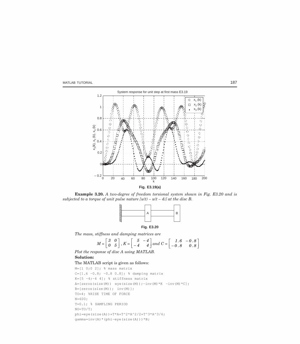
MATLAB TUTORIAL 187
System response for unit step at first mass E3.191.2
1
0.8
0.6
0.4
0.2
0
– 0.2
x(k
),x
(k),
x(k
)1
23
0 20 40 60 80 100 120 140 160 180 200
x (k)1
x (k)2
x (k)3
k
Fig. E3.19(a)
Example 3.20. A two-degree of freedom torsional system shown in Fig. E3.20 and issubjected to a torque of unit pulse nature [u(t) – u(t – 4)] at the disc B.
A B
Fig. E3.20
The mass, stiffness and damping matrices are
M = 3 00 5
LNM
OQP , K =
5 44 4
−−
LNM
OQP and C =
1 .6 0 . 80 . 8 0 . 8
−−
LNM
OQP
Plot the response of disc A using MATLAB.Solution:The MATLAB script is given as follows:M=[1 0;0 2]; % mass matrix
C=[1.6 -0.8; -0.8 0.8]; % damping matrix
K=[5 -4;-4 4]; % stiffness matrix
A=[zeros(size(M)) eye(size(M));-inv(M)*K -inv(M)*C];
B=[zeros(size(M)); inv(M)];
TO=4; %RISE TIME OF FORCE
N=600;
T=0.1; % SAMPLING PERIOD
NO=TO/T;
phi=eye(size(A))+T*A+T^2*A^2/2+T^3*A^3/6;
gamma=inv(A)*(phi-eye(size(A)))*B;
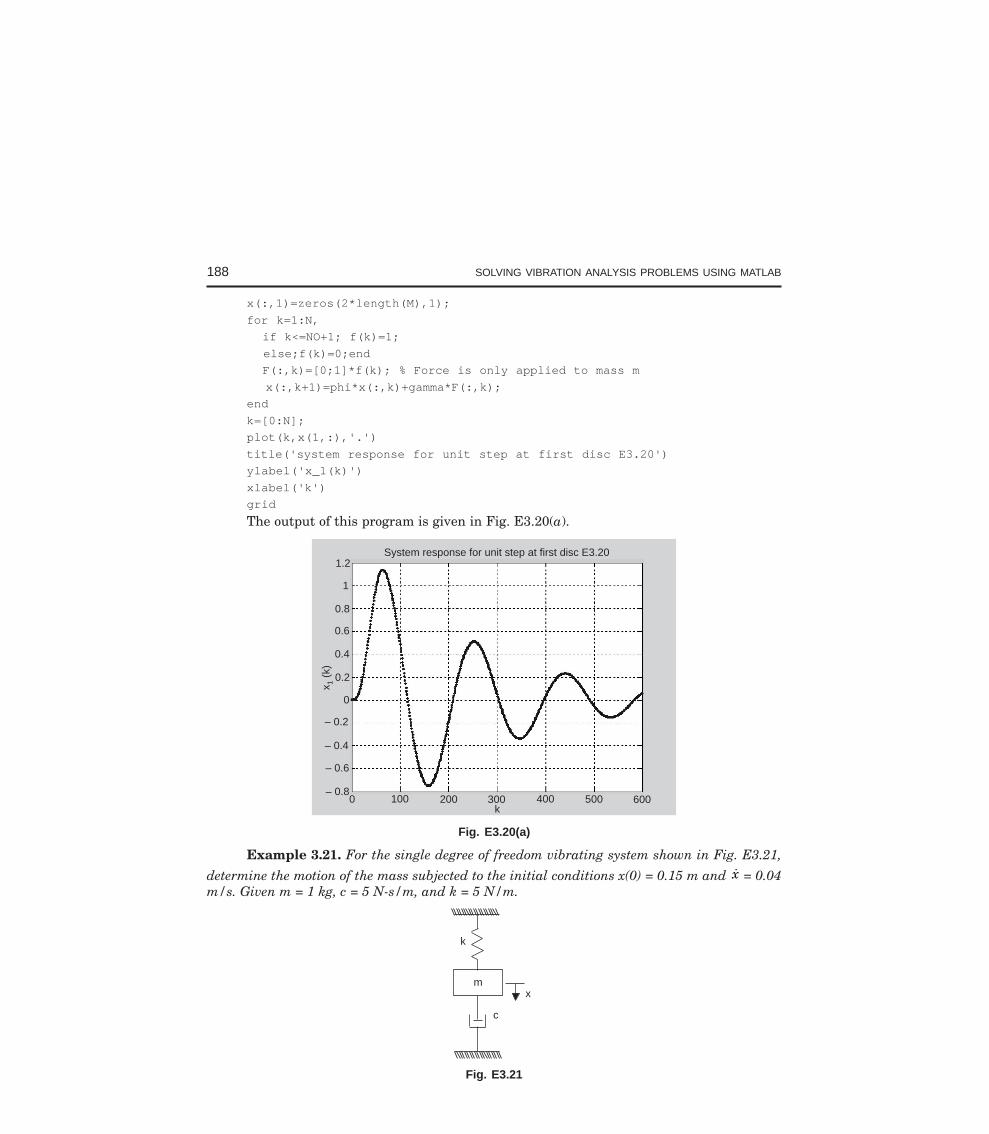
188 SOLVING VIBRATION ANALYSIS PROBLEMS USING MATLAB
x(:,1)=zeros(2*length(M),1);
for k=1:N,
if k<=NO+1; f(k)=1;
else;f(k)=0;end
F(:,k)=[0;1]*f(k); % Force is only applied to mass m
x(:,k+1)=phi*x(:,k)+gamma*F(:,k);
end
k=[0:N];
plot(k,x(1,:),'.')
title('system response for unit step at first disc E3.20')
ylabel('x_1(k)')
xlabel('k')
grid
The output of this program is given in Fig. E3.20(a).
System response for unit step at first disc E3.201.2
1
0.8
0.4
0.2
0
– 0.2
– 0.4
0.6
– 0.6
– 0.80 100 200 300 400 500 600
k
x(k
)1
Fig. E3.20(a)
Example 3.21. For the single degree of freedom vibrating system shown in Fig. E3.21,
determine the motion of the mass subjected to the initial conditions x(0) = 0.15 m and x = 0.04m/s. Given m = 1 kg, c = 5 N-s/m, and k = 5 N/m.
m
k
c
x
Fig. E3.21
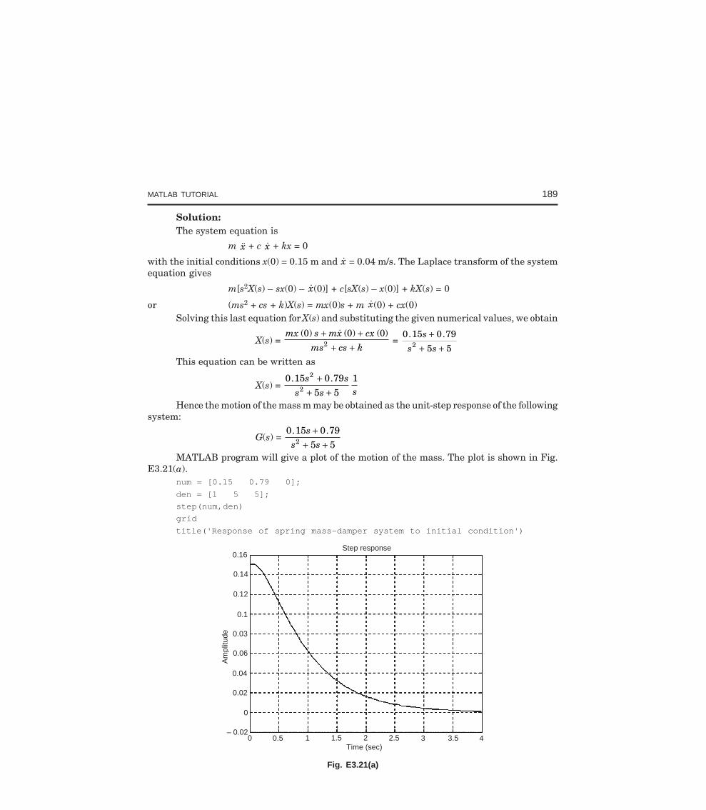
MATLAB TUTORIAL 189
Solution:The system equation is
m x + c x + kx = 0
with the initial conditions x(0) = 0.15 m and x = 0.04 m/s. The Laplace transform of the systemequation gives
m[s2X(s) – sx(0) – x(0)] + c[sX(s) – x(0)] + kX(s) = 0
or (ms2 + cs + k)X(s) = mx(0)s + m x(0) + cx(0)Solving this last equation for X(s) and substituting the given numerical values, we obtain
X(s) = mx s mx cx
ms cs k
( ) ( ) ( )0 0 02
+ ++ +
= 0 15 0 79
5 52. .s
s s
++ +
This equation can be written as
X(s) = 0 15 0 79
5 512
2
. .s ss s s
++ +
Hence the motion of the mass m may be obtained as the unit-step response of the followingsystem:
G(s) = 0 15 0 79
5 52
. .ss s
++ +
MATLAB program will give a plot of the motion of the mass. The plot is shown in Fig.E3.21(a).
num = [0.15 0.79 0];
den = [1 5 5];
step(num,den)
grid
title('Response of spring mass-damper system to initial condition')
Step response0.16
0.14
0.12
0.1
0.03
0.06
0.04
0.02
0
– 0.020
Am
plitu
de
0.5 1 1.5 2.5 3.52 3 4Time (sec)
Fig. E3.21(a)
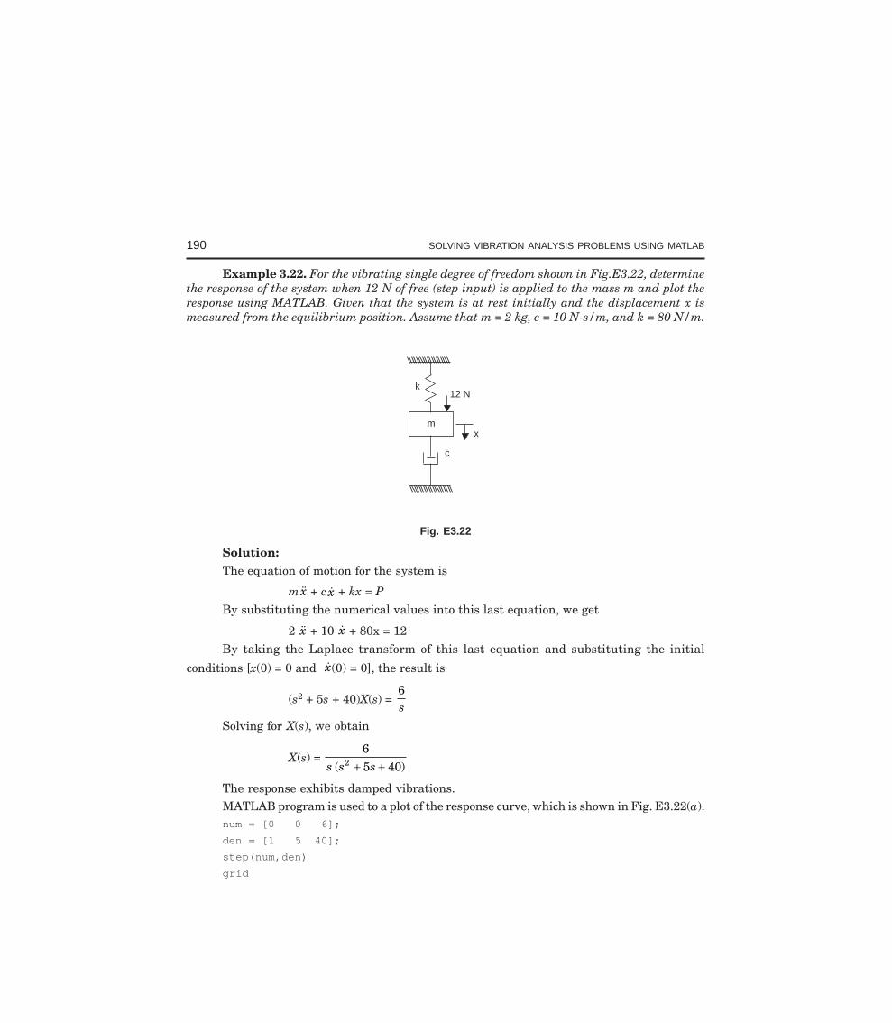
190 SOLVING VIBRATION ANALYSIS PROBLEMS USING MATLAB
Example 3.22. For the vibrating single degree of freedom shown in Fig.E3.22, determinethe response of the system when 12 N of free (step input) is applied to the mass m and plot theresponse using MATLAB. Given that the system is at rest initially and the displacement x ismeasured from the equilibrium position. Assume that m = 2 kg, c = 10 N-s/m, and k = 80 N/m.
12 N
m
k
c
x
Fig. E3.22
Solution:The equation of motion for the system is
m x + c x + kx = PBy substituting the numerical values into this last equation, we get
2 x + 10 x + 80x = 12By taking the Laplace transform of this last equation and substituting the initial
conditions [x(0) = 0 and x(0) = 0], the result is
(s2 + 5s + 40)X(s) = 6s
Solving for X(s), we obtain
X(s) = 65 402s s s( )+ +
The response exhibits damped vibrations.MATLAB program is used to a plot of the response curve, which is shown in Fig. E3.22(a).num = [0 0 6];
den = [1 5 40];
step(num,den)
grid

MATLAB TUTORIAL 191
Step response
Am
plitu
de
0.2
0.18
0.16
0.14
0.12
0.1
0.08
0.06
0.04
0.02
01.5 2.5210.50
Time (sec)
Fig. E3.22(a)
Example 3.23. For the mechanical system shown in Fig. E3.23, obtain the response x0(t)when xi(t) is a unit step displacement input. Assume that k1 = 2 N/m, k2 = 4 N/m, c1 = 1 N-s/m,and c2 = 2 N-s/m.
k1
c2
x
c1
k2
x0
Fig. E3.23
Solution:The transfer function X0(s)/Xi(s) is given by
X sX si
0 ( )( ) =
ck
sck
s
ck
sck
sck
s
1
1
2
2
1
1
2
2
2
1
1 1
1 1
+FHG
IKJ +FHG
IKJ
+FHG
IKJ +FHG
IKJ +
Substitution of the given numerical values yields
X sX si
0 ( )( )
= ( . ) ( . )
( . ) ( . )0 5 1 0 5 1
0 5 1 0 5 1s s
s s s+ +
+ + + = 0 25 10 25 2 1
2
2
..
s ss s
+ ++ + =
s ss s
2
2
4 48 4
+ ++ +
The MATLAB program is used to obtain the unit-step response is given below:
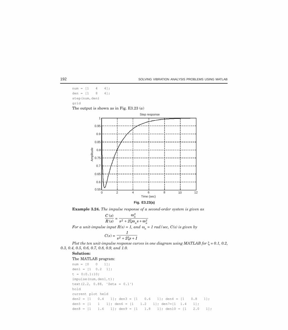
192 SOLVING VIBRATION ANALYSIS PROBLEMS USING MATLAB
num = [1 4 4];
den = [1 8 4];
step(num,den)
grid
The output is shown as in Fig. E3.23 (a)
Step response1
0.95
0.9
0.85
0.8
0.75
0.7
0.65
0.6
0.550 4 6 8 10 12
Time (sec)2
Am
plitu
de
Fig. E3.23(a)
Example 3.24. The impulse response of a second-order system is given as
C sR s
( )( )
= ω
ξω ωn2
2n n
2s 2 s+ +For a unit-impulse input R(s) = 1, and ωn = 1 rad/sec, C(s) is given by
C(s) = 1
s 2 s 12 + +ξPlot the ten unit-impulse response curves in one diagram using MATLAB for ξ = 0.1, 0.2,
0.3, 0.4, 0.5, 0.6, 0.7, 0.8, 0.9, and 1.0.Solution:The MATLAB program:num = [0 0 1];
den1 = [1 0.2 1];
t = 0:0.1:10;
impulse(num,den1,t);
text(2.2, 0.88, 'Zeta = 0.1')
hold
current plot held
den2 = [1 0.4 1]; den3 = [1 0.6 1]; den4 = [1 0.8 1];
den5 = [1 1 1]; den6 = [1 1.2 1]; den7=[1 1.4 1];
den8 = [1 1.6 1]; den9 = [1 1.8 1]; den10 = [1 2.0 1];
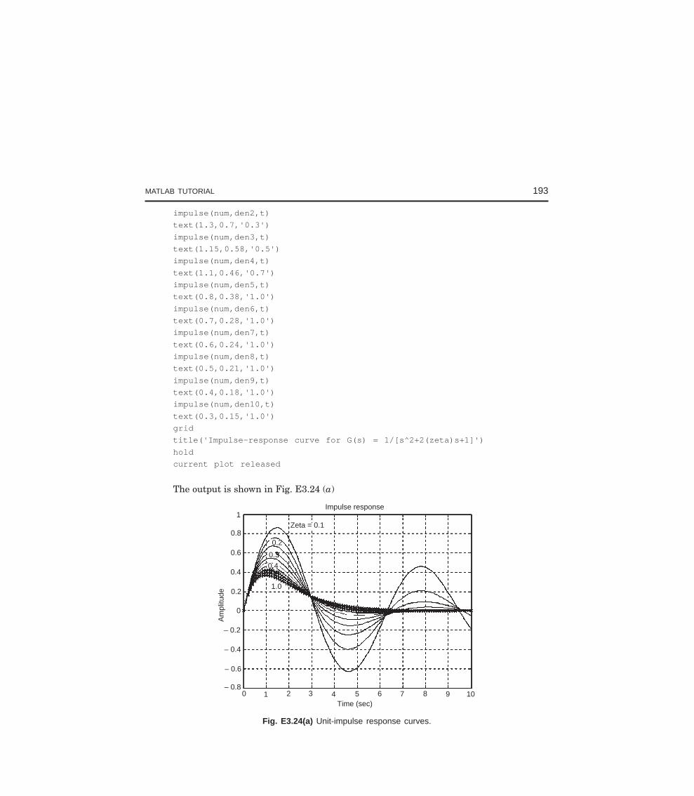
MATLAB TUTORIAL 193
impulse(num,den2,t)
text(1.3,0.7,'0.3')
impulse(num,den3,t)
text(1.15,0.58,'0.5')
impulse(num,den4,t)
text(1.1,0.46,'0.7')
impulse(num,den5,t)
text(0.8,0.38,'1.0')
impulse(num,den6,t)
text(0.7,0.28,'1.0')
impulse(num,den7,t)
text(0.6,0.24,'1.0')
impulse(num,den8,t)
text(0.5,0.21,'1.0')
impulse(num,den9,t)
text(0.4,0.18,'1.0')
impulse(num,den10,t)
text(0.3,0.15,'1.0')
grid
title('Impulse-response curve for G(s) = 1/[s^2+2(zeta)s+1]')
hold
current plot released
The output is shown in Fig. E3.24 (a)
Impulse response1
0.8
0.6
0.4
0.2
0
– 0.2
– 0.4
– 0.6
– 0.80 1 2 3 4 5 6 7 8 9 10
Time (sec)
Zeta = 0.1
Am
plitu
de
0.2
0.3
0.4
1.0
Fig. E3.24(a) Unit-impulse response curves.
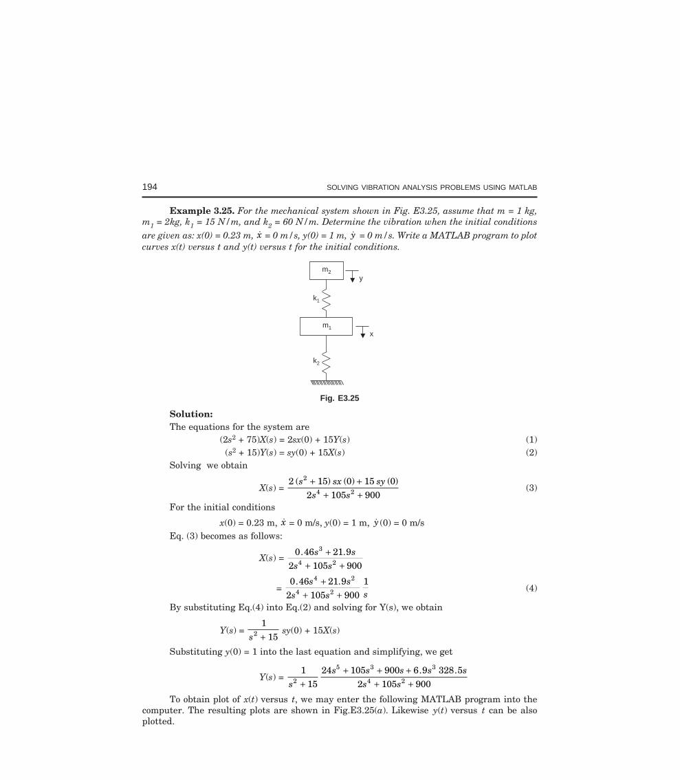
194 SOLVING VIBRATION ANALYSIS PROBLEMS USING MATLAB
Example 3.25. For the mechanical system shown in Fig. E3.25, assume that m = 1 kg,m1 = 2kg, k1 = 15 N/m, and k2 = 60 N/m. Determine the vibration when the initial conditionsare given as: x(0) = 0.23 m, x = 0 m/s, y(0) = 1 m, y = 0 m/s. Write a MATLAB program to plotcurves x(t) versus t and y(t) versus t for the initial conditions.
m1
k1
ym2
k2
x
Fig. E3.25
Solution:The equations for the system are
(2s2 + 75)X(s) = 2sx(0) + 15Y(s) (1) (s2 + 15)Y(s) = sy(0) + 15X(s) (2)
Solving we obtain
X(s) = 2 15 0 15 0
2 105 900
2
4 2
( ) ( ) ( )s sx sys s+ +
+ +(3)
For the initial conditions
x(0) = 0.23 m, x = 0 m/s, y(0) = 1 m, y (0) = 0 m/sEq. (3) becomes as follows:
X(s) = 0 46 21 9
2 105 900
3
4 2
. .s ss s
++ +
= 0 46 21 9
2 105 90014 2
4 2
. .s ss s s
++ +
(4)
By substituting Eq.(4) into Eq.(2) and solving for Y(s), we obtain
Y(s) = 1
152s + sy(0) + 15X(s)
Substituting y(0) = 1 into the last equation and simplifying, we get
Y(s) = 1
1524 105 900 6 9 328 5
2 105 9002
5 3 3
4 2ss s s s s
s s++ + +
+ +. .
To obtain plot of x(t) versus t, we may enter the following MATLAB program into thecomputer. The resulting plots are shown in Fig.E3.25(a). Likewise y(t) versus t can be alsoplotted.
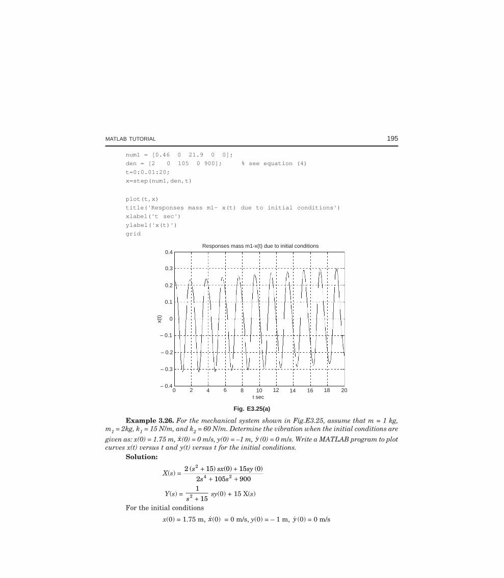
MATLAB TUTORIAL 195
num1 = [0.46 0 21.9 0 0];
den = [2 0 105 0 900]; % see equation (4)
t=0:0.01:20;
x=step(num1,den,t)
plot(t,x)
title('Responses mass m1- x(t) due to initial conditions')
xlabel('t sec')
ylabel('x(t)')
grid
Responses mass m1-x(t) due to initial conditions0.4
0.3
0.2
0.1
0
– 0.1
– 0.2
– 0.3
– 0.40 2 4 6 8 10 12 14 16 18 20
t sec
x(t)
Fig. E3.25(a)
Example 3.26. For the mechanical system shown in Fig.E3.25, assume that m = 1 kg,m1 = 2kg, k1 = 15 N/m, and k2 = 60 N/m. Determine the vibration when the initial conditions are
given as: x(0) = 1.75 m, x(0) = 0 m/s, y(0) = –1 m, y (0) = 0 m/s. Write a MATLAB program to plotcurves x(t) versus t and y(t) versus t for the initial conditions.
Solution:
X(s) = 2 15 0 15 0
2 105 900
2
4 2
( ) ( ) ( )s sx sys s+ +
+ +
Y(s) = 1
152s + sy(0) + 15 X(s)
For the initial conditions
x(0) = 1.75 m, x(0) = 0 m/s, y(0) = – 1 m, y (0) = 0 m/s
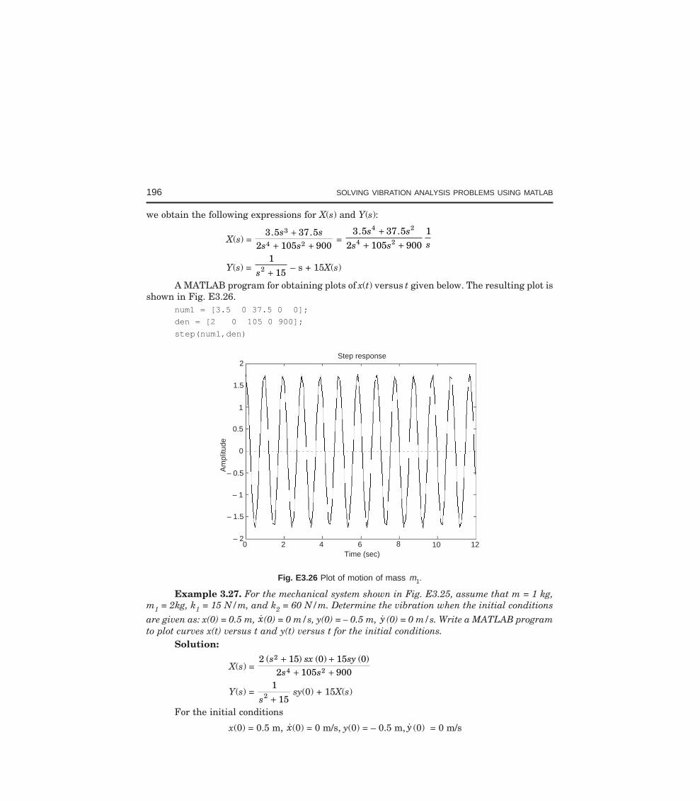
196 SOLVING VIBRATION ANALYSIS PROBLEMS USING MATLAB
we obtain the following expressions for X(s) and Y(s):
X(s) = 3 5 37 5
2 105 900
3
4 2
. .s ss s
++ +
= 3 5 37 5
2 105 90014 2
4 2
. .s ss s s
++ +
Y(s) = 1
152s + – s + 15X(s)
A MATLAB program for obtaining plots of x(t) versus t given below. The resulting plot isshown in Fig. E3.26.
num1 = [3.5 0 37.5 0 0];
den = [2 0 105 0 900];
step(num1,den)
Step response
1.5
2
1
0.5
0
– 0.5
– 1
– 1.5
– 20 2 4 6 8 10 12
Time (sec)
Am
plitu
de
Fig. E3.26 Plot of motion of mass m1.
Example 3.27. For the mechanical system shown in Fig. E3.25, assume that m = 1 kg,m1 = 2kg, k1 = 15 N/m, and k2 = 60 N/m. Determine the vibration when the initial conditions
are given as: x(0) = 0.5 m, x(0) = 0 m/s, y(0) = – 0.5 m, y (0) = 0 m/s. Write a MATLAB programto plot curves x(t) versus t and y(t) versus t for the initial conditions.
Solution:
X(s) = 2 15 0 15 0
2 105 900
2
4 2
( ) ( ) ( )s sx sys s+ +
+ +
Y(s) = 1
152s + sy(0) + 15X(s)
For the initial conditions
x(0) = 0.5 m, x(0) = 0 m/s, y(0) = – 0.5 m, y (0) = 0 m/s
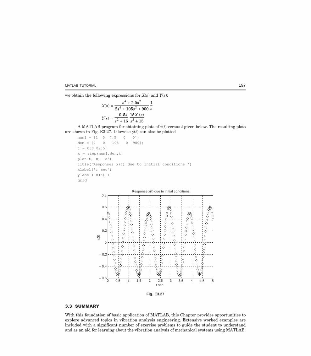
MATLAB TUTORIAL 197
we obtain the following expressions for X(s) and Y(s):
X(s) = s s
s s s
4 2
4 2
7 52 105 900
1++ +
.
Y(s) = −
+ +0 5
15
15
152 2. ( )s
s
X s
sA MATLAB program for obtaining plots of x(t) versus t given below. The resulting plots
are shown in Fig. E3.27. Likewise y(t) can also be plottednum1 = [1 0 7.5 0 0];
den = [2 0 105 0 900];
t = 0:0.02:5;
x = step(num1,den,t)
plot(t, x, 'o')
title('Responses x(t) due to initial conditions ')
xlabel('t sec')
ylabel('x(t)')
grid
Response x(t) due to initial conditions0.8
0.6
0.4
0.2
0
– 0.2
– 0.4
– 0.6
x(t)
0 0.5 1.5 2.5 3.5 4.5 54321t sec
Fig. E3.27
With this foundation of basic application of MATLAB, this Chapter provides opportunities toexplore advanced topics in vibration analysis engineering. Extensive worked examples areincluded with a significant number of exercise problems to guide the student to understandand as an aid for learning about the vibration analysis of mechanical systems using MATLAB.
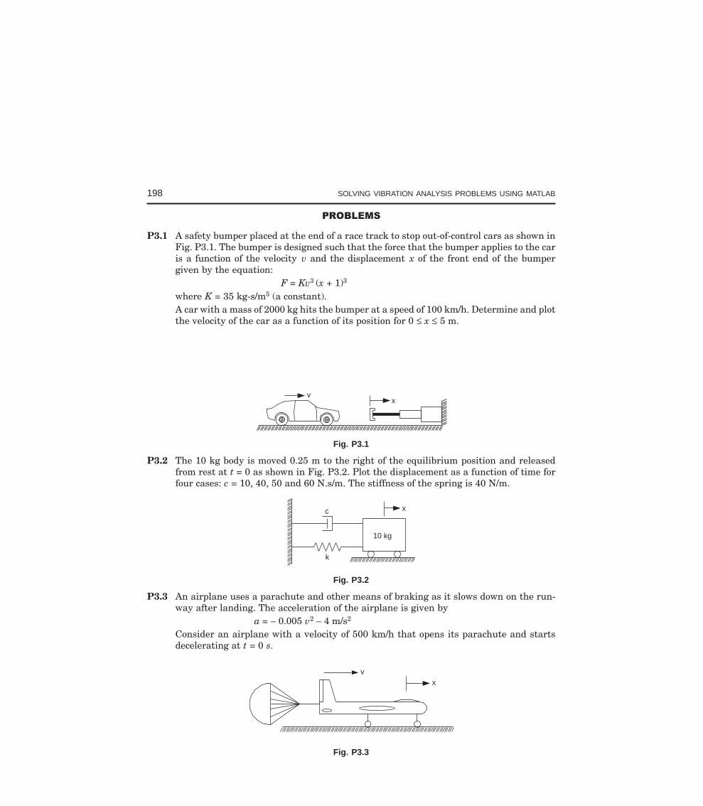
198 SOLVING VIBRATION ANALYSIS PROBLEMS USING MATLAB
P3.1 A safety bumper placed at the end of a race track to stop out-of-control cars as shown inFig. P3.1. The bumper is designed such that the force that the bumper applies to the caris a function of the velocity v and the displacement x of the front end of the bumpergiven by the equation:
F = Kv3 (x + 1)3
where K = 35 kg-s/m5 (a constant).A car with a mass of 2000 kg hits the bumper at a speed of 100 km/h. Determine and plotthe velocity of the car as a function of its position for 0 ≤ x ≤ 5 m.
vx
Fig. P3.1
P3.2 The 10 kg body is moved 0.25 m to the right of the equilibrium position and releasedfrom rest at t = 0 as shown in Fig. P3.2. Plot the displacement as a function of time forfour cases: c = 10, 40, 50 and 60 N.s/m. The stiffness of the spring is 40 N/m.
10 kg
k
c x
Fig. P3.2
P3.3 An airplane uses a parachute and other means of braking as it slows down on the run-way after landing. The acceleration of the airplane is given by
a = – 0.005 v2 – 4 m/s2
Consider an airplane with a velocity of 500 km/h that opens its parachute and startsdecelerating at t = 0 s.
vx
Fig. P3.3
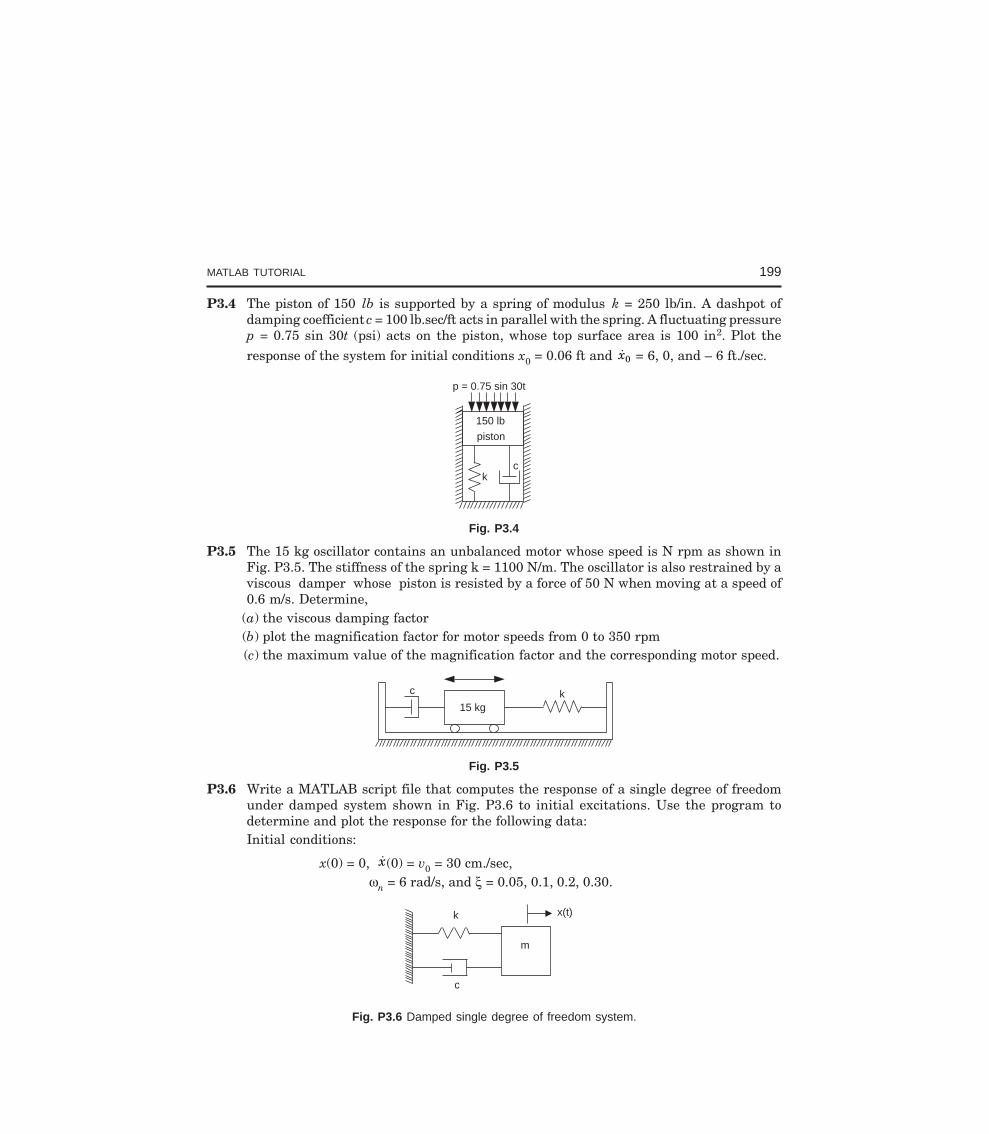
MATLAB TUTORIAL 199
P3.4 The piston of 150 lb is supported by a spring of modulus k = 250 lb/in. A dashpot ofdamping coefficient c = 100 lb.sec/ft acts in parallel with the spring. A fluctuating pressurep = 0.75 sin 30t (psi) acts on the piston, whose top surface area is 100 in2. Plot theresponse of the system for initial conditions x0 = 0.06 ft and x0 = 6, 0, and – 6 ft./sec.
150 lb
piston
kc
p = 0.75 sin 30t
Fig. P3.4
P3.5 The 15 kg oscillator contains an unbalanced motor whose speed is N rpm as shown inFig. P3.5. The stiffness of the spring k = 1100 N/m. The oscillator is also restrained by aviscous damper whose piston is resisted by a force of 50 N when moving at a speed of0.6 m/s. Determine,
(a) the viscous damping factor(b) plot the magnification factor for motor speeds from 0 to 350 rpm(c) the maximum value of the magnification factor and the corresponding motor speed.
15 kgkc
Fig. P3.5
P3.6 Write a MATLAB script file that computes the response of a single degree of freedomunder damped system shown in Fig. P3.6 to initial excitations. Use the program todetermine and plot the response for the following data:Initial conditions:
x(0) = 0, x(0) = v0 = 30 cm./sec, ωn = 6 rad/s, and ξ = 0.05, 0.1, 0.2, 0.30.
m
k
c
x(t)
Fig. P3.6 Damped single degree of freedom system.
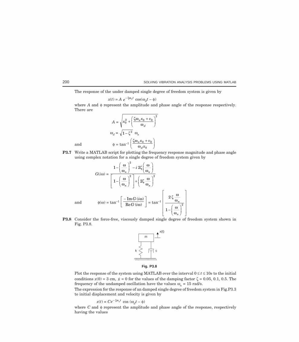
200 SOLVING VIBRATION ANALYSIS PROBLEMS USING MATLAB
The response of the under damped single degree of freedom system is given by
x(t) = A e nt− ξω cos(ωdt – φ)where A and φ represent the amplitude and phase angle of the response respectively.There are
A = xx vn
d02 0 0
2
++F
HGIKJ
ζωω
ωd = 1 2− ζ ωn
and φ = tan–1 ζω
ωn
d
x vx
0 0
0
+FHG
IKJ
P3.7 Write a MATLAB script for plotting the frequency response magnitude and phase angleusing complex notation for a single degree of freedom system given by
G(iω) =
1 2
1 2
2
2 2
−FHG
IKJ −
FHG
IKJ
−FHG
IKJ
L
NMM
O
QPP +
FHG
IKJ
ωω
ζ ωω
ωω
ζ ωω
n n
n n
i
and φ(ω) = tan–1 −L
NMOQP
Im ( )Re ( )
G iG i
ωω = tan–1
2
12
ζ ωω
ωω
n
n−FHG
IKJ
L
N
MMMMM
O
Q
PPPPP
P3.8 Consider the force-free, viscously damped single degree of freedom system shown inFig. P3.8.
m
k c
x(t)
Fig. P3.8
Plot the response of the system using MATLAB over the interval 0 ≤ t ≤ 10s to the initialconditions x(0) = 3 cm, x = 0 for the values of the damping factor ζ = 0.05, 0.1, 0.5. Thefrequency of the undamped oscillation have the values ωn = 15 rad/s.The expression for the response of an damped single degree of freedom system in Fig.P3.3to initial displacement and velocity is given by
x(t) = Ce nt− ζω cos (ωdt – φ)where C and φ represent the amplitude and phase angle of the response, respectivelyhaving the values
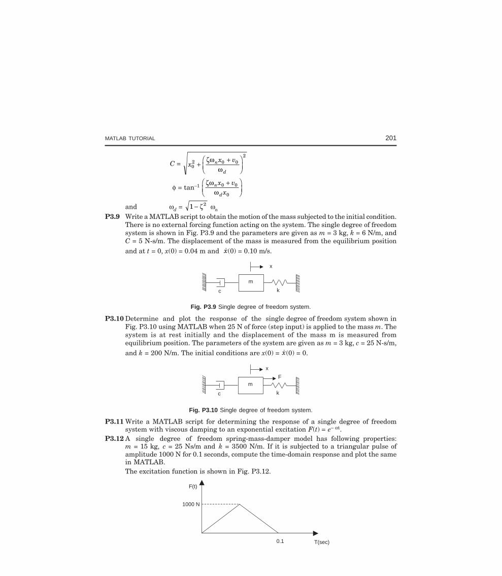
MATLAB TUTORIAL 201
C = xx vn
d02 0 0
2
++F
HGIKJ
ζωω
φ = tan–1 ζω
ωn
d
x vx
0 0
0
+FHG
IKJ
and ωd = 1 2− ζ ωn
P3.9 Write a MATLAB script to obtain the motion of the mass subjected to the initial condition.There is no external forcing function acting on the system. The single degree of freedomsystem is shown in Fig. P3.9 and the parameters are given as m = 3 kg, k = 6 N/m, andC = 5 N-s/m. The displacement of the mass is measured from the equilibrium positionand at t = 0, x(0) = 0.04 m and x(0) = 0.10 m/s.
m
kc
x
Fig. P3.9 Single degree of freedom system.
P3.10 Determine and plot the response of the single degree of freedom system shown inFig. P3.10 using MATLAB when 25 N of force (step input) is applied to the mass m. Thesystem is at rest initially and the displacement of the mass m is measured fromequilibrium position. The parameters of the system are given as m = 3 kg, c = 25 N-s/m,and k = 200 N/m. The initial conditions are x(0) = x(0) = 0.
m
kc
x
F
Fig. P3.10 Single degree of freedom system.
P3.11 Write a MATLAB script for determining the response of a single degree of freedomsystem with viscous damping to an exponential excitation F(t) = e– αt.
P3.12 A single degree of freedom spring-mass-damper model has following properties:m = 15 kg, c = 25 Ns/m and k = 3500 N/m. If it is subjected to a triangular pulse ofamplitude 1000 N for 0.1 seconds, compute the time-domain response and plot the samein MATLAB.The excitation function is shown in Fig. P3.12.
1000 N
0.1
F(t)
T(sec)
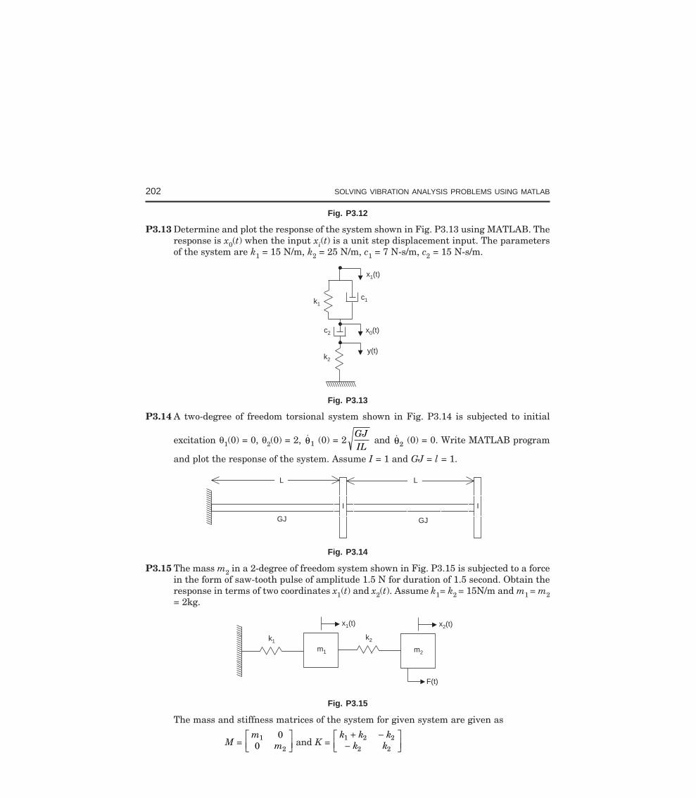
202 SOLVING VIBRATION ANALYSIS PROBLEMS USING MATLAB
Fig. P3.12
P3.13 Determine and plot the response of the system shown in Fig. P3.13 using MATLAB. Theresponse is x0(t) when the input xi(t) is a unit step displacement input. The parametersof the system are k1 = 15 N/m, k2 = 25 N/m, c1 = 7 N-s/m, c2 = 15 N-s/m.
k1c1
x1(t)
k2
c2 x0(t)
y(t)
Fig. P3.13
P3.14 A two-degree of freedom torsional system shown in Fig. P3.14 is subjected to initial
excitation θ1(0) = 0, θ2(0) = 2, θ1 (0) = 2GJIL
and θ2 (0) = 0. Write MATLAB program
and plot the response of the system. Assume I = 1 and GJ = l = 1.
I I
GJ GJ
L L
Fig. P3.14
P3.15 The mass m2 in a 2-degree of freedom system shown in Fig. P3.15 is subjected to a forcein the form of saw-tooth pulse of amplitude 1.5 N for duration of 1.5 second. Obtain theresponse in terms of two coordinates x1(t) and x2(t). Assume k1= k2 = 15N/m and m1 = m2= 2kg.
m1
k1
x (t)1
m2
k2
x2(t)
F(t)
Fig. P3.15
The mass and stiffness matrices of the system for given system are given as
M = m
m1
2
00
LNM
OQP and K =
k k kk k
1 2 2
2 2
+ −−
LNM
OQP
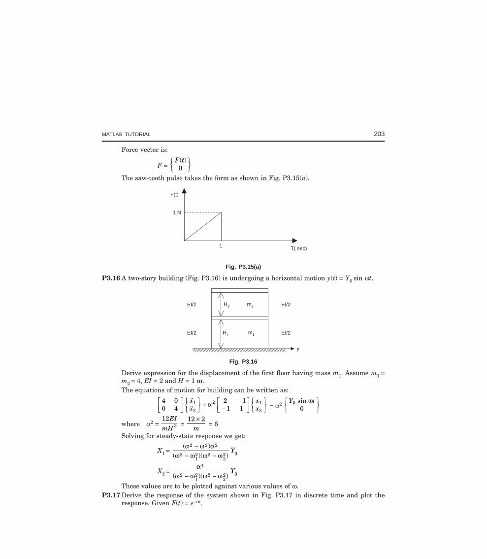
MATLAB TUTORIAL 203
Force vector is:
F = F t( )0
RSTUVW
The saw-tooth pulse takes the form as shown in Fig. P3.15(a).
1 N
1
F(t)
T( sec)
Fig. P3.15(a)
P3.16 A two-story building (Fig. P3.16) is undergoing a horizontal motion y(t) = Y0 sin ωt.
EI/2
EI/2 EI/2
EI/2H1
H2 m2
m1
y
Fig. P3.16
Derive expression for the displacement of the first floor having mass m1. Assume m1 =m2 = 4, EI = 2 and H = 1 m.The equations of motion for building can be written as:
4 00 4
2 11 1
1
2
2 1
2
LNM
OQPRST
UVW + −−
LNM
OQPRST
UVW
xx
xx
α = α2 Y t0
0sin ωRST
UVWwhere α2 =
123
EI
mH =
12 2×m
= 6
Solving for steady-state response we get:
X1 = ( )
( )( )α ω α
ω ω ω ω
2 2 2
212 2
22 0
−− −
Y
X2 = α
ω ω ω ω
4
212 2
22 0( )( )− −
Y
These values are to be plotted against various values of ω.P3.17 Derive the response of the system shown in Fig. P3.17 in discrete time and plot the
response. Given F(t) = e–αt.
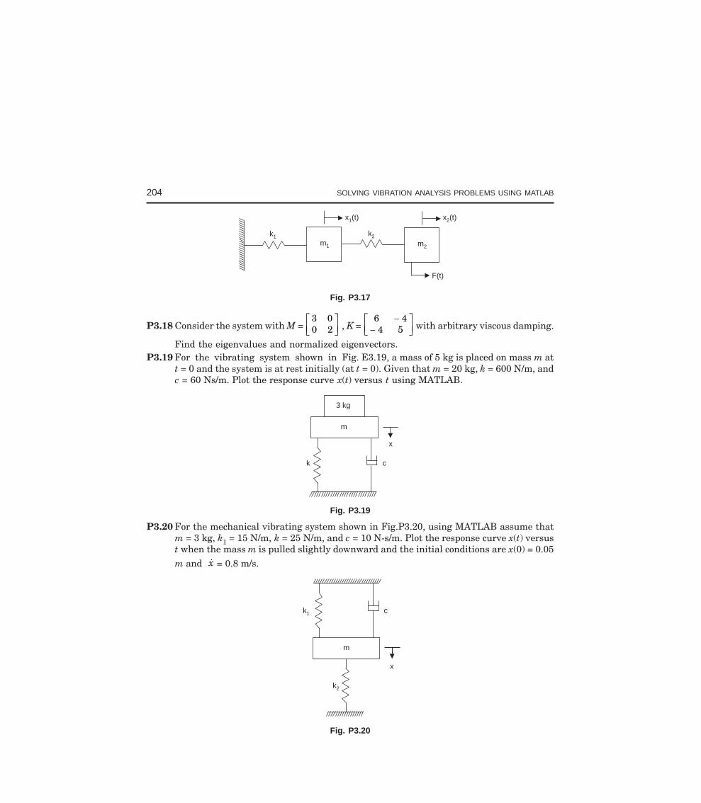
204 SOLVING VIBRATION ANALYSIS PROBLEMS USING MATLAB
k1m1 m2
x (t)1
k2
x (t)2
F(t)
Fig. P3.17
P3.18 Consider the system with M = 3 00 2
LNM
OQP , K =
6 44 5
−−
LNM
OQP with arbitrary viscous damping.
Find the eigenvalues and normalized eigenvectors.P3.19 For the vibrating system shown in Fig. E3.19, a mass of 5 kg is placed on mass m at
t = 0 and the system is at rest initially (at t = 0). Given that m = 20 kg, k = 600 N/m, andc = 60 Ns/m. Plot the response curve x(t) versus t using MATLAB.
m
3 kg
k c
x
Fig. P3.19
P3.20 For the mechanical vibrating system shown in Fig.P3.20, using MATLAB assume thatm = 3 kg, k1 = 15 N/m, k = 25 N/m, and c = 10 N-s/m. Plot the response curve x(t) versust when the mass m is pulled slightly downward and the initial conditions are x(0) = 0.05m and x = 0.8 m/s.
m
k1 c
x
k2
Fig. P3.20
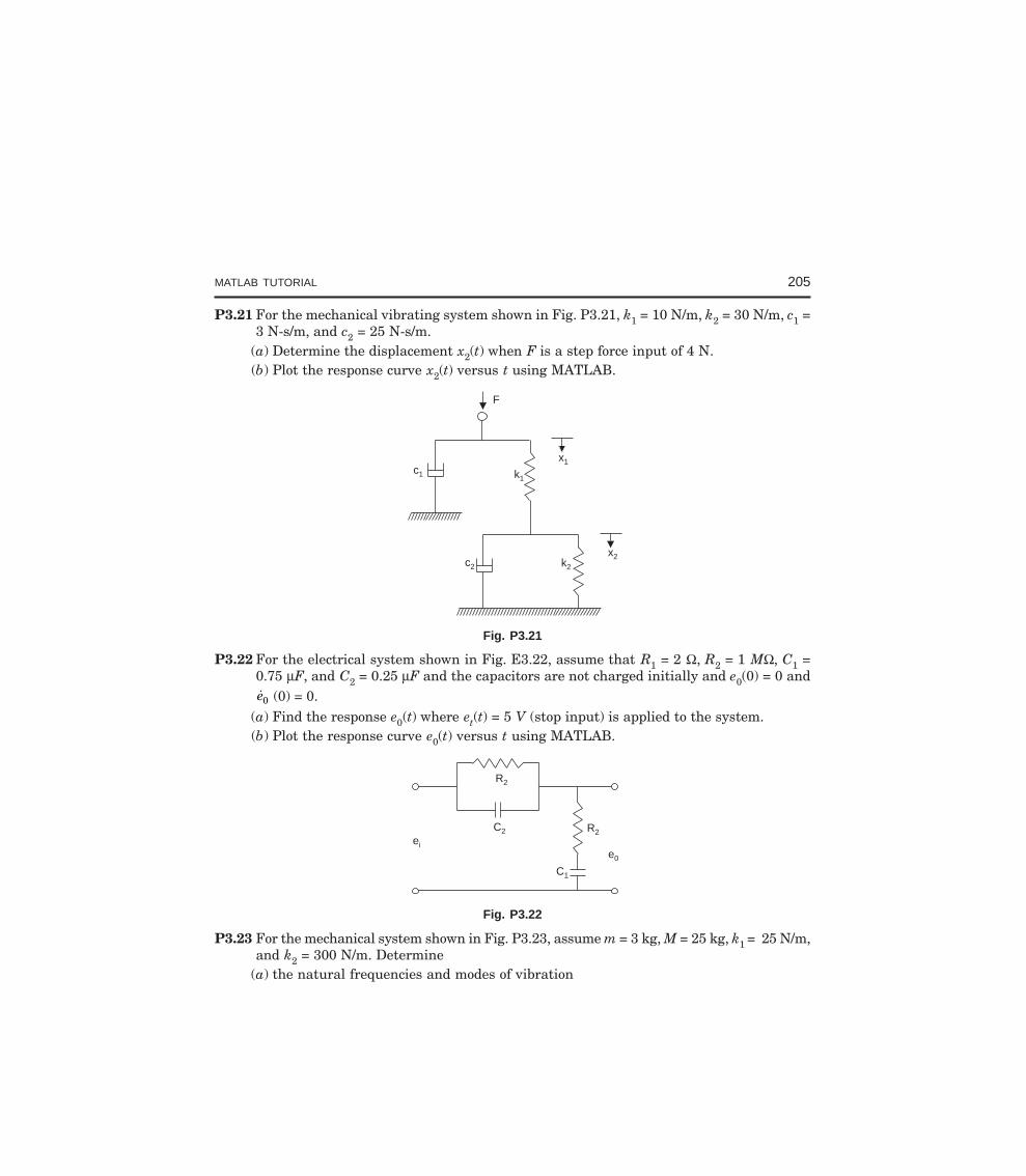
MATLAB TUTORIAL 205
P3.21 For the mechanical vibrating system shown in Fig. P3.21, k1 = 10 N/m, k2 = 30 N/m, c1 =3 N-s/m, and c2 = 25 N-s/m.
(a) Determine the displacement x2(t) when F is a step force input of 4 N.(b) Plot the response curve x2(t) versus t using MATLAB.
c1
F
k1
x1
x2c2 k2
Fig. P3.21
P3.22 For the electrical system shown in Fig. E3.22, assume that R1 = 2 Ω, R2 = 1 MΩ, C1 =0.75 µF, and C2 = 0.25 µF and the capacitors are not charged initially and e0(0) = 0 ande0 (0) = 0.
(a) Find the response e0(t) where et(t) = 5 V (stop input) is applied to the system.(b) Plot the response curve e0(t) versus t using MATLAB.
ei
R2
C2
C1
R2
e0
Fig. P3.22
P3.23 For the mechanical system shown in Fig. P3.23, assume m = 3 kg, M = 25 kg, k1 = 25 N/m,and k2 = 300 N/m. Determine
(a) the natural frequencies and modes of vibration
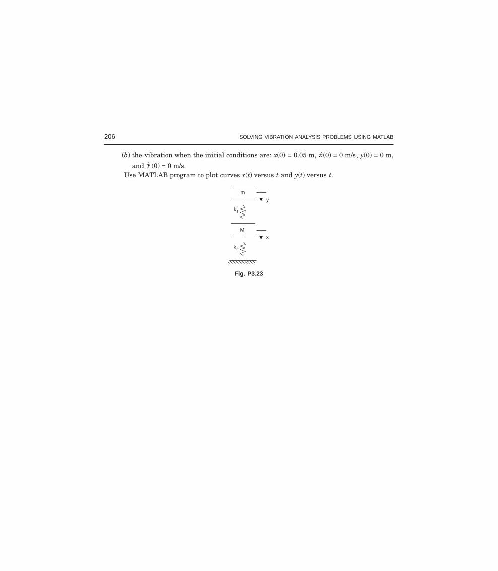
206 SOLVING VIBRATION ANALYSIS PROBLEMS USING MATLAB
(b) the vibration when the initial conditions are: x(0) = 0.05 m, x(0) = 0 m/s, y(0) = 0 m,
and y (0) = 0 m/s.Use MATLAB program to plot curves x(t) versus t and y(t) versus t.
my
Mx
k1
k2
Fig. P3.23
Bibliography
There are several outstanding text and reference books on vibration analysis, numeri-cal methods, and MATLAB that merit consultation for those readers who wish to pursue thesetopics further. Also, there are several publications devoted to presenting research results andin-depth case studies in vibration analysis. The following list is but a representative sample ofthe many excellent references that includes journals and periodicals on vibration analysis,numerical methods, and MATLAB.
Adams, M.L., Rotating Machinery Vibration, Marcel Dekker, New York, NY, 2002.
Anderson, J.F., and Anderson, M.B., Solution of Problems in Vibrations, LongmanScientific and Technical, Essex, UK, 1987.
Anderson, R.A., Fundamentals of Vibrations, Macmillan, New York, NY, 1967.
Balachandran, B., and Magrab, E.B., Vibrations, Brooks/Cole, Pacific Grove, CA, 2004.
Barker, J.R., Mechanical and Electrical Vibrations, Wiley, New York, NY, 1964.
Beards, C.F., Structural Vibration Analysis, Ellis Harwood, U.K, 1983.
Beards, G.F., Vibrations and Control System, Ellis Harwood, UK, 1988.
Benaroya, H., Mechanical Vibrations, Prentice Hall, Upper Saddle River, NJ, 1998.
Bendat, J.S., and Piersol, A.G., Engineering Applications of Correlation and SpectralAnalysis, Wiley, New York, 1980.
Bendat, J.S., and Piersol, A.G., Measurement and Analysis of Random Vibration Data,Wiley, New York, NY, 1965.
Bendat, J.S., and Piersol, A.G., Random Data, Wiley, New York, NY, 1986.
Bendat, J.S., and Piersol, A.G., Random Data: Analysis and Measurement Procedures,Wiley, New York, NY, 1971.
Beranek, L.L., and Ver, I.L., Noise and Vibration Control Engineering: Principles andApplications, Wiley, New York, NY, 1992.
Beranek, L.L., Noise and Vibration Control, McGraw Hill, New York, NY, 1971.
Berg, G.V., Elements of Structural Dynamics, Prentice Hall, Englewood cliffs, NJ, 1989.
Bernhard, R.K., Mechanical Vibrations, Pitman Publishing, 1943.
207
208 SOLVING VIBRATION ANALYSIS PROBLEMS USING MATLAB
Bhat, R.B., and Dukkipati, R.V., Advanced Dynamics, Narosa Publishing House, NewDelhi, India, 2001.
Bickley, W.G., and Talbot, A., Vibrating Systems, Oxford University Press, Oxford,1961.
Bishop, R. E.D., Vibration, Cambridge University Press, Cambridge, England, 1979.
Bishop, R.E.D., and Gladwell, G.M.L., The Matrix Analysis of Vibration, CambridgeUniversity Press, Cambridge, England, 1965.
Bishop, R.E.D., and Johnson, D.C., Vibration Analysis Tables, Cambridge UniversityPress, Cambridge, England, 1956.
Bishop, R.F.D., and Johnson, D.C., The Mechanics of Vibration, Cambridge UniversityPress, New York, NY, 1960.
Blevins, R.D., Formulas for Natural Frequencies and Mode Shapes, R.E. Krieger,Melbourne, FL, 1987.
Broch, J.F., Mechanical Vibrations and Shock Measurements, Larson & Sons,Copenhagen, Denmark, 1980.
Brommundt, E., Vibration of Continuous Systems, CISM, Udine, Italy, 1969.
Burton, R., Vibration and Impact, Dover Publications, New York, NY, 1958.
Bykhovsky, I., Fundamentals of Vibration Engineering, MIR Publications, 1972.
Centa, G., Vibration of Structures and Machines, Springer Verlag, New York NY, 1993.
Chen, Y., Vibrations: Theoretical Methods, Addison-Wesley, Reading, MA, 1966.
Church, A.H., Mechanical Vibrations, 2nd ed., Wiley, New York, NY, 1963.
Cole, E.B., The Theory of Vibrations for Engineers, Crosby Lockwood, 1950.
Crafton, P.A., Shock and Vibration in Linear Systems, Harper & Row, New York, NY,1961.
Crandall, S.H., and Mark, W.D., Random Vibration in Mechanical Systems, AcademicPress, New York, NY, 1963.
Crandall, S.H., Random Vibration, MIT Press, Cambridge, MA, 1963.
De Silva, C.W., Vibration: Fundamentals and Practice, CRC Press, Boca Raton, FL,2000.
Del Pedro, M., and Pahud, P., Vibration Mechanics, Kluwer Academic Publishers,Dordrecht, Netherlands, 1989.
Den Hartog. J.P., Mechanical Vibrations, 4th ed., McGraw Hill, New York, NY, 1956.
Dimarogonas, A.D., and Haddad, S.D., Vibration for Engineers, Prentice Hall,Englewood cliffs, NJ, 1992.
Dimarogonas, A.D., Vibration for Engineers, 2nd ed., Prentice Hall, Englewood cliffs,NJ, 1996.
Dukkipati, R.V., Advanced Engineering Analysis, Narosa Publishing House, New Delhi,India, 2006.
Dukkipati, R.V., Advanced Mechanical Vibrations, Narosa Publishing House, New Delhi,India, 2006.
BIBLIOGRAPHY 209
Dukkipati, R.V., and Amyot, J.R., Computer Aided Simulation in Railway VehicleDynamics, Marcel-Dekker, New York, NY, 1988.
Dukkipati, R.V., and Srinivas, J., A Text Book of Mechanical Vibrations, PrenticeHall of India, New Delhi, India, 2005.
Dukkipati, R.V., and Srinivas, J., Vibrations: Problem Solving Companion, NarosaPublishing House, New Delhi, India, 2006.
Dukkipati, R.V., Vehicle Dynamics, Narosa Publishing House, New Delhi, India, 2000.
Dukkipati, R.V., Vibration Analysis, Narosa Publishing House, New Delhi, India, 2005.
Fertis, D.G., Mechanical and Structural Vibrations, Wiley, New York, NY, 1995.
Garg, V.K., and Dukkipati, R.V., Dynamics of Railway Vehicle Systems, AcademicPress, New York, NY, 1984.
Garg, V.K., and Dukkipati, R.V., Dynamics of Railway Vehicle Systems, Academic Press,New York, NY, 1984.
Genta, G., Vibration of Structures and Machines, Springer-Verlag, New York, NY, 1992.
Ginsberg, J.H., Mechanical and Structural Vibrations, Wiley, New York, NY, 2001.
Gorman, D.J., Free Vibration Analysis of Beams and Shafts, Wiley, New York, NY, 1975.
Gorman, D.J., Free Vibration Analysis of Rectangular Plates, Elsevier, 1982.
Gough, W., Richards, J.P.G., and Williams, R.P., Vibrations and Waves, Wiley, NewYork, NY, 1983.
Gross, E.E., Measurement of Vibration, General Radio, 1955.
Grover, G.K., Mechanical Vibration, Nem Chand and Bros. Roorkee, 1972.
Haberman, C.M., Vibration Analysis, Merril, Columbus, OH, 1968.
Hansen, H.M., and Chenea, P.F., Mechanics of Vibration, Wiley, New York, NY, 1952.
Harris, C.M., Crede, C.E., Shock and Vibration Handbook, 4th ed., McGraw Hill, NewYork, NY, 199
Hatter, D.H., Matrix Computer Methods of Vibration Analysis, Wiley, New York, NY,1973.
Hayashi, C., Nonlinear Oscillations in Physical Systems, McGraw Hill. New York, NY,1964.
Hurty, W.C., and Rubenstein, M.F., Dynamics of Structures, Prentice Hall, NJ, 1964.
Huston, R., and Josephs, H., Dynamics of Mechanical Systems, CRC Press, Boca Raton,FL, 2002.
Inman, D.J., Vibration with Control Measurement and Stability, Prentice Hall, Englewoodcliffs, NJ, 1989.
Jackson, C., The Practical Vibration Primer, Gulf Publishing, Houston, TX, 1979.
Jacobsen, L.S., and Ayre, R.S., Engineering Vibrations, McGraw Hill, New York, 1958.
James, M.L., Smith, G.M., Wolford, J.C., and Whaley, P.W., Vibration of Mechanicaland Structural Systems, Harper and Row, 1989.
Jones, D.S., Electrical and Mechanical Oscillations, Routledge and Kegan, London, 1961.
210 SOLVING VIBRATION ANALYSIS PROBLEMS USING MATLAB
Karnopp, D.C., Margolis, D.L., and Rosenberg, R.C., System Dynamics, 3rd ed., WileyInter Science, New York NY, 2000.
Kelly, S.G., Fundamentals of Mechanical Vibration, McGraw Hill, New York, NY, 1993.
Kelly, S.G., Theory and Problems of Mechanical Vibrations, Schaum’s Outline Series,McGraw Hill, New York, NY, 1996.
Kimball, A.L., Vibration Prevention in Engineering, Wiley, New York, NY, 1932.
Lalanne, M., Berthier, P., and Der Hagopian, J., Mechanical Vibrations for Engineers,Wiley, New York, NY, 1983.
Lancaster, P., Lambda-Matrices and Vibrating Systems, Pergamon, 1966.
Loewy, R.G., and Piarulli, V.J., Dynamics of Rotating Shafts, Naval Publication, 1969.
Manley, R.G., Fundamentals of Vibration Study, Wiley, New York, NY, 1942.
Marguerre, K., and Wolfel, H., Mechanics of Vibration, Sitjthoff and Noordhoff, 1979.
Mclachlan, N.W., Theory of Vibration, Dover publications, 1951.
Meirovitch, L., Analytical Methods in Vibrations, Macmillan, New York, NY, 1967.
Meirovitch, L., Elements of Vibration Analysis, 2nd ed., McGraw Hill, New York, NY,1986.
Meirovitch, L., Introduction to Dynamics and Control, Wiley, New York, NY, 1985.
Meirovitch, L., Methods of Analytical Dynamics, McGraw Hill, New York, NY, 1970.
Meirovitch, L., Principles and Techniques of Vibrations, Prentice Hall, Upper SaddleRiver, NJ, 1997.
Minorosky, M., Nonlinear Oscillations, Van Nostrand, Princeton, NJ, 1962.
Moretti, P.M., Modern Vibrations Primer, CRC Press, Boca Raton, FL, 2002.
Morrill, B., Mechanical Vibration, The Ronald Press, 1937.
Morrow, C.T., Shock and Vibration Engineering, Wiley, New York, NY, 1963.
Morse, P.M., Vibration and Sound, McGraw Hill, New York, NY, 1948.
Muller, P.C., and Schiehlen, W.O., Linear Vibrations, Martinus Nighoff, 1985.
Myklestad, N.O., Fundamentals of Vibration Analysis, McGraw Hill, New York, NY,1956.
Nakra, B.C., Yadava, G.S., and Thurestadt, L., Vibration Measurement and Analysis,NPC, New Delhi, India, 1989.
Nashif, A.D., Jones, D.I.G., and Henderson, J.P., Vibration Damping, Wiley, NewYork, NY, 1985.
Nayfeh, A.H., and Mook, D.T., Nonlinear Oscillations, Wiley, New York, NY, 1979.
Newland, D.E., An Introduction to Random Vibrations and Spectral Analysis, 2nd ed.,Longman, 1984.
Newland, D.E., Mechanical Vibration Analysis and Computation, Longman, 1989.
Newland, D.E., Random Vibrations and Spectral Analysis, 2nd ed., Longman, London,1984.
BIBLIOGRAPHY 211
Nigam, N.C., Introduction to Random Vibrations, MIT Press, 1983.
Norton, M.P., Fundamentals of Noise and Vibration Analysis for Engineers, CambridgeUniversity Press, Cambridge, 1989.
Pain, H.J., The Physics of Vibrations and Waves, Wiley, New York, NY 1983.
Pippard, A.B., The Physics of Vibration, Cambridge University Press, Cambridge, 1978.
Piszek, K., and Niziol, J., Random Vibrations of Mechanical Systems, Ellis Horwood,1986.
Prentis, J.M., and Leckie, F.A., Mechanical Vibrations: An Introduction to MatrixMethods, Longman, 1963.
Ramamurti, V., Mechanical Vibration Practice With Basic Theory, CRC Press, BocaRaton, FL, 2000.
Rao, J.S., Advanced Theory of Vibration, Wiley, New York, NY, 1991.
Rao, J.S., and Dukkipati, R.V., Mechanism and Machine Theory, 2nd ed., Wiley Eastern,New Delhi, India, 1992.
Rao, J.S., and Gupta, K., Introductory Course on Theory and Practice of MechanicalVibrations, Wiley Eastern, New Delhi, India, 1984.
Rao, S.S., Mechanical Vibrations, 3rd ed., Addison Wesley, Reading, MA, 1995.
Rocard, V., General Dynamics of Vibrations, Unger, New York, NY, 1960.
Seto, W.W., Theory and Problems of Mechanical Vibrations, Schaum series, McGrawHill, New York, NY, 1964.
Shabana, A.A., Theory of Vibration: An Introduction, Springer-Verlag, New York, NY,1991.
Shabana, A.A., Theory of Vibration: Discrete and Continuous Systems, Springer, NewYork, NY, 1991.
Smith, J.D., Vibration Measurement and Analysis, Butterworths, 1989.
Snowdon, J.C., Vibration and Shock in Damped Mechanical Systems, Wiley, New York,NY, 1968.
Srinivasan, P., Mechanical Vibration Analysis, Tata McGraw Hill, New Delhi, India,1982.
Steidel, R.F., An Introduction to Mechanical Vibrations, 3rd ed., Wiley, New York, NY,1981.
Stoker, J.J., Nonlinear Vibrations, Inter science, New York, NY, 1950.
Thompson, J.M.T., and Stewart, H.B., Nonlinear Dynamics and Chaos, Wiley, NewYork NY, 1986.
Thomson, W.T., and Dahleh, M.D., Theory of Vibrations with Applications, 5th ed.,Prentice Hall, Englewood Cliffs, NJ, 199.
Thornson, D.L., Mechanics Applied to Vibrations and Balancing, Wiley, New York, NY,1940.
Timoshenko, S., Young, D.H., and Weaver, W., Vibration Problems in Engineering,5th ed., Wiley, New York, NY 1990.
212 SOLVING VIBRATION ANALYSIS PROBLEMS USING MATLAB
Timoshenko, S.P., and Young, D.H., Advanced Dynamics, McGraw Hill, New York,NY, 1948.
Timoshenko, S.P., Vibrations in Engineering, D. Van Nostrand, New York, NY, 1955.
Tong, K.N., Theory of Mechanical Vibration, Wiley, New York, NY, 1960.
Tse, F.S., Morse, I.E., and Hinkle, R.T., Mechanical Vibrations, Allyn and Bacon,Boston, MA, 1963.
Tuplin, W.A., Torsional Vibration, Wiley, New York, NY, 1934.
Van Santen, G.W., Mechanical Vibration, Macmillan, New York, NY, 1998.
Vernon, J.B., Linear Vibration Theory, Wiley, New York, NY, 1967.
Vierck, R.K., Vibration Analysis, 2nd ed., Harper & Row, New York, NY, 1979.
Volterra, E., and Zachmanoglon, E.C., Dynamics of Vibrations, Merrill, 1965.
Wallace, R.H., Understanding and Measuring Vibrations, Springer, New York, NY, 1970.
Walshaw, A.C., Mechanical Vibrations with Applications, Ellis Harwood, 1984.
Weaver, W., Timoshenko, S.P., and Young, D.H., Vibration Problems in Engineering,5th ed., Wiley, New York, NY, 1990.
Wilson, W.K., Practical Solution of Torsional Vibration Problems, Vol.1, Wiley, NewYork, NY, 1949
Wilson, W.K., Practical Solution of Torsional Vibration Problems, Vol.2, Wiley, NewYork, NY, 1949
Wowk, V., Machinery Vibration: Measurement and Analysis, McGraw Hill, New York,NY, 1991.
Akai, T.J., Applied Numerical Methods for Engineers, Wiley, New York, NY, 1993.
Ali, R., “Finite difference methods in vibration analysis”, Shock and Vibration Digest,Vol.15, March 1983, pp.3-7.
Atkinson, K.E., An Introduction to Numerical Analysis, 2nd ed., Wiley, New York, NY,1993.
Atkinson, L.V., and Harley, P.J., Introduction to Numerical Methods with PASCAL,Addison Wesley, Reading, MA, 1984.
Ayyub, B.M., and McCuen, R.H., Numerical Methods for Engineers, Prentice Hall,Upper Saddle River, New Jersey, NJ, 1996.
Bathe, K.J., and Wilson, E.L., Numerical Methods in Finite Element Analysis, PrenticeHall, Englewood Cliffs, NJ, 1976.
Belytschko, T., “Explicit Time Integration of Structure-Mechanical Systems”, in J. Donea(Ed.), Advanced Structural Dynamics, Applied Science Publishers, London, England,1980, pp.97-122.
Belytschko, T., and Mullen, R., “Stability of Explicit-Implicit Mesh Partitions in TimeIntegration”, International Journal for Numerical Methods in Engineering, Vol.12,1975, pp.1575-1586.
BIBLIOGRAPHY 213
Belytschko, T., Schoeberle. D.F., “On the Unconditional Stability of An ImplicitAlgorithm for Nonlinear Structural Dynamics”, Journal of Applied Mechanics, Vol.42,1975, pp.865-869.
Belytschko. T., Holmes, N., and Mullen, R., “Explicit Integration Stability, SolutionProperties, Cost”, Finite-Element Analysis of Transient Nonlinear Structural Behavior,ASME, AMD Vol.14, 1975.
Bhat, R.B., and Dukkipati, R.V., Advanced Dynamics, Narosa Publishing House, NewDelhi, India, 2001.
Brice, C., Luther, H.A and Wilkes, J. O., Applied Numerical Methods, New York, NY,1969.
Chapra, S.C., Numerical Methods for Engineers with Software and ProgrammingApplications, 4th ed., McGraw Hill, New York, NY, 2002.
Clough, R.W., and Penzien, J., Dynamics of Structures, McGraw Hill, New York, NY,1975.
Conte, S.D., and DeBoor, C.W., Elementary Numerical Analysis: An AlgorithmApproach, 2nd ed., McGraw Hill, New York, NY, 1972.
Cornwell, R.E., Craig, R.R. Jr., and Johnson, C.P., “On the Application of the Mode-Acceleration Method to Structural Engineering Problems”, Earthquake Engineeringand Structural Dynamics, Vol. 11, 1983, pp. 679-688.
Dukkipati, R.V., Ananda Rao, M., and Bhat, R.B., Computer Aided Analysis andDesign of Machine Elements, Narosa Publishing House, New Delhi, India, 2000.
Dukkipati, R.V., and Amyot, J.R., Computer Aided Simulation in Railway VehicleDynamics, Marcel-Dekker, New York, NY, 1988.
Dukkipati, R.V., Vehicle Dynamics, Narosa Publishing House, New Delhi, India, 2000.
Epperson, J.F., An Introduction to Numerical Methods and Analysis, Wiley, New York,NY, 2001.
Fallow, S.J., “A Computer Program to Find Analytical Solutions of Second Order LinearDifferential Equations”, International Journal for Numerical Methods in Engineering,Vol.6, 1973, pp. 603-606.
Fausett, L.V., Applied Numerical Analysis using MATLAB, Prentice Hall, Upper SaddleRiver, New Jersey, NJ, 1999.
Fausett, L.V., Numerical Methods using MATHCAD, Prentice Hall, Upper Saddle River,New Jersey, NJ, 2002.
Ferziger, J.H., Numerical Methods for Engineering Applications, 2nd ed., Wiley, NewYork, NY, 1998.
Forbear, C. E., Introduction to Numerical Analysis, Addison Wesley, Reading, MA, 1969.
Garg, V.K., and Dukkipati, R.V., Dynamics of Railway Vehicle Systems, Academic Press,New York, NY, 1984.
Gerald, C.F., and Wheatley, P.O., Applied Numerical Analysis, 3rd ed., Addison Wesley,Reading, MA, 1984.
214 SOLVING VIBRATION ANALYSIS PROBLEMS USING MATLAB
Goudreau, G.L., and Taylor, R.L., “Evaluation of Numerical Integration Methods inElastodynamics”, Computational Methods in Applied Mechanics and Engineering, Vol.2, 1973, pp. 69-97.
Hanselman, D., and Littlefield, B.R., Mastering MATLAB 6, Prentice Hall, UpperSaddle River, New Jersey, NJ, 2001.
Hildebrand, F.B., Introduction to Numerical Analysis, McGraw-Hill, New York, NY,1956.
Hojjat, A., Gere, J.M., and Weaver, W., “Algorithm For Nonlinear Structural Dynamics”,Journal of the Structural Division, ASCE, Feb.1978, pp. 263-279.
Houbolt, J.C., “A Recurrence Matrix Solution for the Dynamic Response of ElasticAircraft”, Journal of Aeronautical Sciences, Vol.17, 1950, pp. 540-550, 594.
Huges, T.J.R., “A Note on the Stability of Newmark’s Algorithm in Nonlinear StructuralDynamics”, International Journal for Numerical Methods in Engineering, Vol.11, 1976,pp. 383-386.
Hurty, W.C., and Rubinstein, M.F., Dynamics of Structures, Prentice Hall, EnglewoodCliffs, NJ, 1970.
Jennings, A., and Orr, D.R.L., “Application of the Simultaneous Iteration Method toUndamped Vibration Problems”, International Journal for Numerical Methods inEngineering, Vol.3, 1971, pp.13-24.
Key, S.W., “Transient Response by Time Integration: Review of Implicit and ExplicitOperators”, in J. Donea (Ed.), Advanced Structural Dynamics, Applied SciencePublishers, London, England, 1980.
Krieg, R.D., “Unconditional Stability in Numerical Time Integration Methods”, Journalof Applied Mechanics, Vol.40, 1973, pp.417-421.
Lambert, J.D., Numerical Methods for Ordinary Differential Equations—The InitialValue Problems, Wiley, New York, NY, 1991.
Lau, P.C.M., “Finite Difference Approximation for Ordinary Derivatives”, InternationalJournal for Numerical Methods in Engineering, Vol.17, 1981, pp.663-678.
Leech, J.W., Hsu, P.T., Mack, E.W., “Stability of A Finite-Difference Method for SolvingMatrix Equations”, AIAA Journal, Vol.3, 1965, pp. 2172-2173.
Levy, S., and Kroll W.D., “Errors Introduced by Finite Space and Time Increments inDynamics Response Computation”, Proceedings of the First U.S. National Congress ofApplied Mechanics, 1951, pp.1-8.
Levy, S., and Wilkinson, J.P.D., The Component Element Method in Dynamics withApplication to Earthquake Engineering, McGraw Hill, New York, NY, 1976.
Lindfield, G., and Penny, J., Numerical Methods using MATLAB, 2nd ed., PrenticeHall, Upper Saddle River, New Jersey, NJ, 2000.
Magrab, E.B., An Engineers Guide to MATLAB, Prentice Hall, Upper Saddle River, NewJersey, NJ, 2001.
Mathews, J.H., and Fink, K., Numerical Methods using MATLAB, 3rd ed., PrenticeHall, Upper Saddle River, New Jersey, NJ, 1999.
BIBLIOGRAPHY 215
McNamara, J.F., “Solution Schemes for Problems of Nonlinear Structural Dynamics”,Journal of Pressure Vessel Technology, ASME, May 1974, pp.96-102.
Nakamara, S., Numerical Analysis and Graphic Visualization with MATLAB, 2nd ed.,Prentice Hall, Upper Saddle River, New Jersey, NJ, 2002.
Nakamura, S., Computational Methods in Engineering and Science, Wiley, New York,NY, 1977.
Newmark, N.M., “A Method of Computation for Structural Dynamics”, ASCE Journalof Engineering Mechanics Division, Vol. 85, 1959, pp. 67-94.
Park, K.C., “An improved Stiffly Method for Direct Integration of Non-Linear StructuralDynamics Equations”, Journal of the Applied Mechanics, ASME, June 1975, pp.464-470.
Penman, E.D., “A Numerical Method for Coupled Differential Equations”, InternationalJournal for Numerical Methods in Engineering, Vol. 41972, pp. 587-596.
Rao, S.S., Applied Numerical Methods for Engineers and Scientists, Prentice Hall, UpperSaddle River, New Jersey, NJ, 2002.
Reali, M., Rangogni, R., and Pennati, V., “Compact Analytic Expressions of Two-Dimensional Finite Difference Forms”, International Journal for Numerical Methodsin Engineering, Vol. 20, 1984, pp.121-130.
Recktenwald, G.W., Introduction to Numerical Methods and MATLAB—Implementationand Applications, Prentice Hall, Upper Saddle River, New Jersey, NJ, 2001.
Romanelli, M.J., “Runge-Kutta Method for the Solution of Ordinary DifferentialEquations”, in Mathematical Methods for Digital Computers, A. Ralston and H.S. Wilf(eds.), Wiley, New York, NY, 1965.
Tillerson, J.R., Stricklin, J.A., and Haisler, W.E., “Numerical Methods for the Solutionof Nonlinear Problems in Structural Analysis”, ASME Winter Annual Meeting, Detroit,MI, Nov. 11-15, 1973.
Timoshenko, S.P., Young, D.H., and Weaver, W. Jr., Vibration Problems inEngineering, 4th ed., Wiley, New York, 1974.
Wah, T., and Colcote, L.R., Structural Analysis by Finite Difference Calculus, VanNostrand Reinhold, New York, NY, 1970.
Wang, P.C., Numerical and Matrix Methods in Structural Mechanics, Wiley, New York,NY, 1966.
Wilson, E.L., Farhoomand, I., and Bathe, K.J., “Nonlinear Dynamic Analysis ofComplex Structures”, International Journal of Earthquake Engineering and StructuralDynamics, Vol. 1, 1973, pp. 241-252.
Chapman, S.J., MATLAB Programming for Engineers, 2nd ed., Brooks/Cole, ThomsonLearning, Pacific Grove, CA, 2002.
Dabney, J.B., and Harman, T.L., Mastering SIMULINK 4, Prentice Hall, Upper SaddleRiver, NJ, 2001.
216 SOLVING VIBRATION ANALYSIS PROBLEMS USING MATLAB
Djaferis, T.E., Automatic Control- The Power of Feedback using MATLAB, Brooks/Cole,Thomson Learning, Pacific Grove, CA, 2000.
R.V. Dukkipati, Solving Engineering Mechanics Problems with MATLAB, New AgeInternational (P) Ltd., New Delhi, India, ISBN: 81-224-1809-0, 2007.
R.V. Dukkipati, MATLAB for Engineers, New Age International (P) Ltd., New Delhi,India, ISBN: 81-224-1809-0, 2007.
R.V. Dukkipati, Analysis and Design of Control Systems using MATLAB, New AgeInternational (P) Ltd., New Delhi, India, ISBN: 81-224-1809-0, 2006.
R.V. Dukkipati, Solving Engineering System Dynamics Problems with MATLAB, NewAge International (P) Ltd., New Delhi, India, 2007.
Etter, D.M., Engineering Problem Solving with MATLAB, Prentice-Hall, Englewood Cliffs,NJ, 1993.
Gardner, J.F., Simulation of Machines using MATLAB and SIMULINK, Brooks/Cole,Thomson Learning, Pacific Grove, CA, 2001.
Harper, B. D., Solving Dynamics Problems in MATLAB, 5th ed, Wiley, New York, 2002.
Harper, B. D., Solving Statics Problems in MATLAB, 5th ed, Wiley, New York, 2002.
Herniter, M.E., Programming in MATLAB, Brooks/Cole, Pacific Grove, CA, 2001.
Karris, S.T., Signals and Systems with MATLAB Applications, Orchard Publications,Fremont, CA, 2001.
Leonard, N.E., and Levine, W.S., Using MATLAB to Analyze and Design ControlSystems, Addison-Wesley, Redwood City, CA, 1995.
Lyshevski, S.E., Engineering and Scientific Computations Using MATLAB, Wiley, NewYork, 2003.
Moler, C., The Student Edition of MATLAB for MS-DOS Personal Computers with 3-1/2” Disks, MATLAB Curriculum Series, The MathWorks, Inc., 2002.
Ogata, K., Designing Linear Control Systems with MATLAB, Prentice Hall, Upper SaddleRiver, NJ, 1994.
Ogata, K., Solving Control Engineering Problems with MATLAB, Prentice Hall, UpperSaddle River, NJ, 1994.
Pratap, Rudra., Getting Started with MATLAB- A Quick Introduction for Scientists andEngineers, Oxford University Press, New York, NY, 2002.
Saadat, Hadi., Computational Aids in Control Systems using MATLAB, McGraw Hill,New York, NY, 1993.
Sigman,K., and Davis, T.A., MATLAB Primer, 6th ed, Chapman& Hall/CRCPress, BocaRaton, FL, 2002.
The MathWorks, Inc., SIMULINK, Version 3, The MathWorks, Inc., Natick, MA, 1999.
The MathWorks, Inc., MATLAB: Application Program Interface Reference Version 6,The MathWorks, Inc., Natick, 2000.
The MathWorks, Inc., MATLAB: Control System Toolbox User’s Guide, Version 4, TheMathWorks, Inc., Natick, 1992-1998.
BIBLIOGRAPHY 217
The MathWorks, Inc., MATLAB: Creating Graphical User Interfaces, Version 1, TheMathWorks, Inc., Natick, 2000.
The MathWorks, Inc., MATLAB: Function Reference, The MathWorks, Inc., Natick,2000.
The MathWorks, Inc., MATLAB: Release Notes for Release 12, The MathWorks, Inc.,Natick, 2000.
The MathWorks, Inc., MATLAB: Symbolic Math Toolbox User’s Guide, Version 2, TheMathWorks, Inc., Natick, 1993-1997.
The MathWorks, Inc., MATLAB: Using MATLAB Graphics, Version 6, The MathWorks,Inc., Natick, 2000.
The MathWorks, Inc.,, MATLAB: Using MATLAB, Version 6, The MathWorks, Inc.,Natick, 2000.
AIAA JournalApplied Mechanics ReviewsASCE Journal of Applied MechanicsASME Journal of Applied MechanicsASME Journal of Vibration and AcousticsBulletin of the Japan Society of Solids and StructuresCommunications in Numerical Methods in EngineeringEarthquake Engineering and Structural DynamicsInternational Journal for Numerical Methods in EngineeringInternational Journal for Numerical Methods in EngineeringInternational Journal of Analytical and Experimental Modal AnalysisInternational Journal of Vehicle DesignJournal of Mechanical Systems and Signals, Academic Press, New York, NY, USA.Journal of Sound and Vibration, Academic Press, New York, NY, USAJournal of the Acoustical Society of AmericaJournal of Vibration and Acoustics, American Society of Mechanical Engineers, NewYork, NY, USA.JSME International Journal Series III - Vibration Control EngineeringNoise and Vibration WorldwideShock and Vibration, IOS press, Amsterdam, The NetherlandsVehicle System DynamicsVibrations, Mechanical Systems and Signal Processing.
Shock and Vibration Digest, Sage Science Press, Thousand Oaks, CA, USA.Sound and Vibration, Acoustical Publications, Bay Village, Ohio, USA.


![Theoretical and Experimental Study on Vibration of … · in torsional vibration). ... equations and solving them numerically [1]. He ... codes are written in the MATLAB software](https://img.dokumen.tips/doc/110x75/5b86b1077f8b9a2e3f8d66e4/theoretical-and-experimental-study-on-vibration-of-in-torsional-vibration.jpg)