Solving the linear interval tolerance problem for weight initialization of neural networks

Neural Networks 54 (2014) 17–37

Contents lists available at ScienceDirect

Neural Networks

journal homepage: www.elsevier.com/locate/neunet

Solving the linear interval tolerance problem for weight initializationof neural networksS.P. Adam a,b,∗, D.A. Karras c, G.D. Magoulas d, M.N. Vrahatis a

a Computational Intelligence Laboratory, Department of Mathematics, University of Patras, GR-26110 Patras, Greeceb Department of Computer Engineering, Technological Educational Institute of Epirus, 47100 Arta, Greecec Department of Automation, Technological Educational Institute of Sterea Hellas, 34400 Psahna, Evia, Greeced Department of Computer Science and Information Systems, Birkbeck College, University of London, Malet Street, London WC1E 7HX, UK

a r t i c l e i n f o

Article history:Received 30 March 2013Received in revised form 3 February 2014Accepted 13 February 2014

Keywords:Neural networksWeight initializationInterval analysisLinear interval tolerance problem

a b s t r a c t

Determining good initial conditions for an algorithm used to train a neural network is considereda parameter estimation problem dealing with uncertainty about the initial weights. Interval analysisapproaches model uncertainty in parameter estimation problems using intervals and formulatingtolerance problems. Solving a tolerance problem is defining lower and upper bounds of the intervals sothat the system functionality is guaranteed within predefined limits. The aim of this paper is to showhow the problem of determining the initial weight intervals of a neural network can be defined in termsof solving a linear interval tolerance problem. The proposed linear interval tolerance approach copeswith uncertainty about the initial weights without any previous knowledge or specific assumptions onthe input data as required by approaches such as fuzzy sets or rough sets. The proposed method istested on a number of well known benchmarks for neural networks trained with the back-propagationfamily of algorithms. Its efficiency is evaluated with regards to standard performance measures and theresults obtained are compared against results of a number of well known and established initializationmethods. These results provide credible evidence that the proposedmethod outperforms classical weightinitialization methods.

© 2014 Elsevier Ltd. All rights reserved.

1. Introduction

The purpose of Interval Analysis (IA) is to set upper and lowerbounds on the effect produced on some computed quantity by dif-ferent types of mathematical computing errors (rounding, approx-imation, uncertainty etc.) (Hansen &Walster, 2004; Moore, 1966).Intervals are used to model uncertainty in parameter estimationproblems such as the noise associated with measured data. Suchproblems arise in engineering design or mathematical modelingwhere tolerances in the relevant parameters need to be defined interms of upper and lower bounds so that the desired functionalityis guaranteed within these bounds. The interval-based algorithmsare used to reliably approximate the set of consistent values of pa-rameters by inner and outer intervals and thus take into accountall possible options in numerical constraint satisfaction problems.

∗ Corresponding author at: Computational Intelligence Laboratory, Depart-ment of Mathematics, University of Patras, GR-26110 Patras, Greece. Tel.: +306970806559.

E-mail address: [email protected] (S.P. Adam).

http://dx.doi.org/10.1016/j.neunet.2014.02.0060893-6080/© 2014 Elsevier Ltd. All rights reserved.

The promising features of IA motivated researchers from dif-ferent disciplines to invest in the study and implementation of IAmethods whenever reliable numerical computations are required.Currently, this research field is rapidly growing due to the increas-ing computation power of modern hardware. Examples of applica-tions range from finite element analysis (Degrauwe, Lombaert, &Roeck, 2010) and data analysis (Garloff, Idriss, & Smith, 2007), tostock market forecasting (Hu & He, 2007), reliability of mechanicaldesign (Penmetsa & Grandhi, 2002), and many more. Research inthe area of neural networks has also benefited from IA and a num-ber of efforts utilizing concepts and methods from IA are reportedin the literature. Examples are those by de Weerdt, Chu, and Mul-der (2009) on the use of IA for optimizing the neural network out-put, Ishibuchi and Nii (1998) on the generalization ability of neuralnetworks, Xu, Lam, and Ho (2005) on robust stability criteria forinterval neural networks, Li, Li, and Du (2007) regarding trainingof neural networks, and others.

An important problem encountered when training a neuralnetwork is to determine appropriate initial values for the con-nection weights. Effective weight initialization is associated to

http://dx.doi.org/10.1016/j.neunet.2014.02.006

http://www.elsevier.com/locate/neunet

http://www.elsevier.com/locate/neunet

http://crossmark.crossref.org/dialog/?doi=10.1016/j.neunet.2014.02.006&domain=pdf

mailto:[email protected]

http://dx.doi.org/10.1016/j.neunet.2014.02.006

18 S.P. Adam et al. / Neural Networks 54 (2014) 17–37

performance characteristics such as the time needed to success-fully train the network and the generalization ability of the trainednetwork. Inappropriate weight initialization is very likely to in-crease the training time or even to cause non convergence of thetraining algorithm, while another unfortunate result may be to de-crease the network’s ability to generalize well, especially whentrainingwith back-propagation (BP), a procedure suffering from lo-cal minima, (Hassoun, 1995; Haykin, 1999; Lee, Oh, & Kim, 1991).These are defaults and limitations for having successful practicalapplication of neural networks in real life processes.

The importance manifested by the research community for thissubject has been demonstrated by the number of research workpublished in this area. The proposed approaches can be, roughly,divided into two categories. Methods in the first category performinput data clustering in order to extract significant information(feature vectors or reference patterns) pertaining the pattern spaceand initial connection weights are chosen to be near the centersof these clusters. The main drawback of these methods is thecomputational cost needed to preprocess the input data. Often thiscost may be prohibitive for these methods to be used in real worldapplications. The second category includes those methods that arebased on random selection of initial weights from a subset of Rn,which is an interval defined considering important properties ofthe pattern space and/or the parameters of the training process.

The notion of the interval, underlying random weight selec-tion methods, suggests the idea to use IA in order to deal withuncertainty about the initial weights. Hence, the unknown initialweights are considered to be intervals with unknown bounds. Un-der generally adopted assumptions about the input to any node,the resulting unknown interval quantity is then limited withinspecific upper and lower bounds. Ensuring that scientific compu-tations provide results within guaranteed limits is an issue men-tioned by researchers in IA as a tolerance problem. In consequence,the approach proposed herein gives rise to formulating a linear in-terval tolerance problem which is solved to determine significantintervals for the initial weights. Beaumont and Philippe (2001),Pivkina and Kreinovich (2006), Shary (1995) and other researcherspropose differentmethods for solving a tolerance problem. Besidesformulating the problem of determining initial weights as a linearinterval tolerance problem, we also present here a new algorithmfor defining the required solution to the specific tolerance problem.

The proposed linear interval tolerance approach (LIT-Approach)deals with uncertainty about the initial weights based exclusivelyon numerical information of the patterns without any assumptionon the distribution of the input data. IA provides themeans of han-dling uncertainty in parameters in much the same way this hap-penswith other approaches such as the possibilistic approachwithFuzzy sets (Zadeh, 1978), Evidence theory (Shafer, 1976), Roughsets (Pawlak, 1991) or methods combining properties of these ap-proaches. However, methods using fuzzy sets require parametersof themembership functions to be tuned and eventually some pre-processing of the input data to be done if pertinent input variablesneed to be identified. Moreover, when using rough sets one needsto process the input data in order to deal with the indiscernibil-ity relation and establish upper and lower approximations of theconcepts pertaining the problem, see Bello and Verdegay (2012).Finally, application of the Dempster–Shafer (evidence) theory is amatter of subjective estimation of uncertainty as it assumes thatvalues of belief (or plausibility) are given by an expert. Unlike allthese approaches, the interval computation used for LIT-Approachneeds only elementary statistics of the input data to be computedsuch the sample mean, the sample standard deviation or the me-dian and the quartiles of the sample.

It is worth noting here the approach formulated by Jamett andAcuña (2006) as an interval approach for weight initialization.The solution proposed ‘‘solves the network weight initialization

problem, performing an exhaustive search for minima by meansof interval arithmetic. Then, the global minimum is obtained oncethe search has been limited to the region of convergence’’. For theexperimental evaluation proposed, interval weights are initiallydefined as wide as necessary (with amplitudes up to 106). Inaddition, the IA solution adopted by these researchers extends todefining an interval version of the gradient descent procedure. Onthe contrary, the method presented in this paper uses IA conceptsonly for computing effective intervals for the initial weights andtherefore it is not computationally expensive.

The sections of this paper are organized as follows. Section 2is devoted to a presentation of the IA concepts underpinning theLIT-Approach. Section 3 presents the analysis of LIT-Approachincluding both theoretical results and the weight initializationalgorithm. Section 4 is dedicated to the experimental evaluationof our approach and its comparison with well known initializationprocedures. Finally, Section 5 summarizes the paper with someconcluding remarks.

2. Interval analysis and the tolerance problem

2.1. Interval arithmetic

The arithmetic defined on sets of intervals, rather than sets ofreal numbers is called interval arithmetic. An interval or intervalnumber I is a closed interval [a, b] ⊂ R of all real numbers be-tween (and including) the endpoints a and b, with a 6 b. The termsinterval number and interval are used interchangeably. Whenevera = b the interval is said to be degenerate, thin or even point inter-val. An intervalX maybe also denoted as

X, X

, [X] or even [XL, XU ]

where subscripts L and U stand for lower and upper bounds respec-tively. Interval variables may be uppercase or lowercase, (Alefeld& Mayer, 2000). In this paper, identifiers for intervals and intervalobjects (variables or vectors) will be denoted with boldface lower-case such as x, y, z and boldface uppercase notation will be usedfor matrices, e.g. X . Lowercase letters will be used for the squarebracketed notation of intervals [x, x], or the elements of an inter-val as a set. An interval [x, x] where x = −x is called a symmetricinterval. Finally, if x = [x, x] then the following notation will beused in this paper.

rad(x) = (x − x)/2, is the radius of the interval xmid(x) = (x + x)/2, is themidpoint

(meanvalue) of the interval x|x| = max{|x|, |x|}, is the absolute value

(magnitude) of the interval xIR, denotes the set of real intervalsIRn, denotes the set of n-dimensional vectors of real intervals

Let � denote one of the elementary arithmetic operators {+, −, ×,÷} for the simple arithmetic of real numbers x, y. If x, y denote realintervals then the four elementary arithmetic operations are de-fined by the rule

x � y = { x � y | x ∈ x, y ∈ y}. (1)

This definition guarantees that x�y ∈ x�y for any arithmetic oper-ator and any values of x and y. In practical calculations each intervalarithmetic operation is reduced to operations between real num-bers. If x = [x, x] and y = [y, y] then it can be shown that the abovedefinition produces the following intervals for each arithmetic op-eration:

x + y = [x + y, x + y] (2a)

x − y = [x − y, x − y] (2b)

S.P. Adam et al. / Neural Networks 54 (2014) 17–37 19

x × y =min

xy, xy, xy, xy

,max

xy, xy, xy, xy

(2c)

x ÷ y = x ×1y, with (2d)

1y

=

1y,1y

, provided that 0 ∈

y, y

. (2e)

The usual algebraic laws of arithmetic operations applied to realnumbers need to be reconsidered regarding finite arithmetic onintervals. For instance, a non-degenerate (thick) interval has noinverse with respect to addition and multiplication. So, if x, y arenon-degenerate intervals then,

x + y = z ; x = z − y, (3a)

x × y = z ; x = z ×1y. (3b)

The following sub-distributive law holds for non-degenerate inter-vals x, y and z ,

x × (y + z) ⊆ x × y + x × z. (4)

One may easily verify that the usual distributive law holds if x is apoint interval or if both y and z are point intervals. Hereafter, themultiplication operator × will be omitted as in usual algebraic ex-pressions with real numbers. A very important property of intervalarithmetic operations is that,

if a, b, c, d ∈ IR and a ⊆ b, c ⊆ d (5)then a � c ⊆ b � d, � ∈ {+, −, ×, ÷}.

This property is the inclusion isotony of interval arithmetic oper-ations and it is considered to be the fundamental principle of IA.More details on interval arithmetic and its extensions can be foundin Alefeld and Mayer (2000), Hansen andWalster (2004) and Neu-maier (1990).

2.2. Interval linear systems

An interval linear system is a system of the form,

Ax = b (6)

where A ∈ IRm×n, also notedA,A

, is an m-by-n matrix of real

intervals, b ∈ IRm, also notedb, b

, is anm-dimensional vector of

real intervals and x is the n-dimensional vector of unknown inter-val variables. Solving a system of linear interval equations has at-tracted the interest of several researchers in the field of IA formorethan forty years. Initially, research focused on systemswith squareinterval matrices (A ∈ IRn×n) and a number of different methodsfor studying and solving such systems have been proposed.

To solve the above system of interval linear equations Ax = b,generally, means to compute the solution set defined as

(A, b) = {x ∈ Rn| Ax = b for real A ∈ A, b ∈ b}. (7)

That is,

(A, b) is the set of all solutions for allmatrices A ∈ Awithreal elements and all vectors b ∈ b having real number compo-nents. This set is generally not an interval vector but a rather com-plicated set that is usually impractical to define and use (Hansen& Walster, 2004). In practice, defining this solution set resultedin proposing methods such as the interval versions of Gaussianelimination or the Gauss–Seidel method which compute vectorsthat bound

(A, b). Note that these interval algorithms differ

significantly from corresponding point algorithms as they use pre-conditioning with a point matrix for the algorithms to be effec-tive (Hansen & Walster, 2004; Neumaier, 1990). Other frequentlyused methods are those based on the Rump/Krawczyk iteration(Krawczyk, 1969; Rump, 2001).

An important issue was to define the narrowest interval vectorcontaining the solution set

(A, b). This interval vector is called

the hull of the solution set. Determining the hull is a problem that isNP-hard as shown by Heindl, Kreinovich, and Lakeyev (1998), andso, in general, methods try to compute only outer bounds for thehull. Other important research results include: the work by Rohn(2003) on the solvability of systems of linear interval equationswith rectangular matrices, the algorithm proposed by Hansen(2006), to solve over-determined systems and the work presentedby Kubica (2010) on interval methods for under-determined non-linear systems.

For such methods one may refer to Alefeld and Herzberger(1983), Hansen (1992), Hansen and Walster (2004), Kearfott(1996), Kreinovich, Lakeyev, Rohn, and Kahl (1997), Neumaier(1990). The number of different methods proposed to solve sys-tems of linear interval equations underlines the importance ofthe subject, especially regarding the difficulty to generally iden-tify the hull of the solution set of such a system. Research efforthas been dedicated on the evaluation of different methods solvingsystems of linear interval equations. Important works on this mat-ter include Goldsztejn (2007), Neumaier (1984), Ning and Kearfott(1997), Rohn (1993).

2.3. Tolerance problem and the tolerance solution set

The tolerance problem arises in engineering design and sys-tem modeling and refers to the estimation of the tolerance of cer-tain parameters of a system or a device so that its behavior i.e. itsoutput is guaranteed within specified bounds. In mathematicalterms, if F : Rn

→ Rm is the mapping relating variables x =

(x1, x2, . . . , xn)⊤ with output parameters y = (y1, y2, . . . , ym)⊤,then the tolerance problem is associatedwith the computation of adomain for the variables of F such that the corresponding y = F (x)lie within some predefined range, (Neumaier, 1986, 1990).

In Shary (2002) the tolerance problem is described as aparticular problem related with the analysis of a system. Usingintervals and quantifier formalism to model uncertainty, about asystem’s parameters, Shary defines three types of solutions to thegeneral input-state-output equation describing a system. Thesesolutions are sets of values providing answers to different issues ofsystems analysis. Hence, according to Shary (2002), for the intervalequation F (a, x) = b of a system with n unknown parametersx ∈ Rn, there are three particular cases of the general AE-solutionset:

• the United solution set consisting of the solutions of all pointequation systems of the form F

a, x

= bwith a ∈ a and b ∈ b,

• the Controllable solution set containing all point vectors x suchthat for any b ∈ b one can find the right a ∈ a such thatFa, x

= b, and finally,

• the Tolerable (or Tolerance) solution set formed by all pointvectors x such that for any a ∈ a the image F

a, x

∈ b.

In the case of a static linear system F has the form of the intervallinear system Ax = b and the solution set defined by (7) is theUnited solution set. Using the notation introduced in Shary (1995)the solution sets defined previously are:

United solution set:∃∃

(A, b) = {x ∈ Rn| (∃A ∈ A)(∃b ∈ b)(Ax = b)}. (8)

Controllable solution set:∃∀

(A, b) = {x ∈ Rn| (∀b ∈ b)(∃A ∈ A)(Ax = b)}. (9)


Tolerance solution set:∀∃

(A, b) = {x ∈ Rn| (∀A ∈ A)(∃b ∈ b)(Ax = b)} (10)

⊆

(A, b) = {x ∈ Rn| Ax ⊆ b}. (11)

Both the Controllable and the Tolerance solution sets are subsetsof the more general United solution set. The specific uncertaintyproblem defines which of the above solution sets contains thesolution of the problem. With respect to the assumption that Fdescribes the input–output relation of a static linear system, thetolerance solution set provides answers to the question whetherthere are input signals x to the system such that the output Axremainswithin specified limits b. Moreover, it is worth noting herethat the elements of the solution sets, as defined previously, are notjust points in Rn but they may be intervals in IRn as well (Pivkina& Kreinovich, 2006; Shary, 1995).

3. Weight initialization with the LIT-Approach

3.1. Random selection of initial weights

Random initialization of connection weights seems to be themost widely used approach for real world applications. A numberof approaches such as those presented in this section claim thereputation to provide improvement in BP convergence speed andavoidance of bad local minima, (Nguyen &Widrow, 1990; Wessels& Barnard, 1992). Unless differently defined, hereafter din denotesthe number of inputs to a node.

Fahlman (1988) studies on random weight initializationtechniques resulted in the use of a uniform distribution over theinterval [−1.0, 1.0]. This seems to constitute a simplified approachfor use in any problem without further hypotheses.

Boers and Kuiper (1992) initialize the weights using a uniformdistribution over the interval

−3/

√din, 3/

√din. This interval is

defined so that the stimulus of any node is located around theorigin of the axes where the sigmoid activation function has itssteepest slope. This interval is the same as the one defined by theconventional method of Wessels and Barnard (1992). However,in order to avoid false local minima detected when applying thisconventional method, Wessels and Barnard (1992) also propose amore refined method adopting a different strategy for the input-to-hidden layer connections and for the hidden-to-output layerconnections.

Bottou (1988) defines the interval−a/

√din, a/

√din, where a

is chosen so that the weight variance corresponds to the points ofthe maximal curvature of the activation function. For the logisticsigmoid activation function a is set to be approximately equal to2.38 and 0.66 for the hyperbolic tangent. Criticismon this approachconcerns the fact that it was not compared against other methods.

Kim and Ra (1991) calculated a lower bound for the initiallength of the weight vector of a neuron to be

√η/din where η is

the learning rate used by the training procedure.Smieja (1991) based on the study of the hyperplanes dynamics,

proposes uniformly distributed weights normalized to the magni-tude 2/

√din for each node. The thresholds for the hidden units are

initialized to a random value in the interval−

√din/2,

√din/2

and the thresholds of the output nodes are set to zero.

Drago and Ridella (1992) proposed a method aiming to avoidflat regions in the error surface in an early stage of training.Their method is called statistically controlled activation weightinitialization (SCAWI). They determine the maximum magnitudeof the weights through statistical analysis. They show thatthe maximum magnitude of the weights is a function of theparalyzed neuron percentage (PNP), which is in turn related to

the convergence rate. By determining the optimal range of PNPthrough computer simulations, the maximum magnitude of theweights can be obtained. The weights are uniformly distributedover the interval [−r, r] with r = 1.3/

1 + niv2 for the hidden

layer nodes and r = 1.3/√1 + 0.3nh for the output layer nodes.

Here, ni denotes the number of inputs to the network and nh isthe number of nodes in the hidden layer. In addition v2 is themean of the expectation of the quadratic values of the inputs,v2

= 1/nini

i=1 E[I2i ].Nguyen and Widrow (1990) proposed a simple modification of

the widely used random initialization process of Fahlman (1988).The weights connecting the output units to the hidden units areinitialized with small random values over the interval [−0.5, 0.5].The initial weights at the first layer are designed to improve thelearning capabilities of the hidden units. Using the magnificationfactor defined by the relation, ρ = 0.7H1/N whereH is the numberof hidden units and N is the number of inputs, the weights arerandomly selected in the interval [−1, 1] and then scaled by v =

ρv/ ∥ v ∥where v is the first layer weight vector. Results obtainedby Pavelka and Procházka (2004), provide significant experimentalevidence on the superiority of Nguyen–Widrow’s method againsttypical random initialization techniques.

In addition to the above, a number of interesting methodsrelated to this context have been formulated by Chen andNutter (1991), LeCun (1993), Osowski (1993), Schmidhuber andHochreiter (1996), YamandChow (1995, 1997), aswell as by othersresearchers.

Despite the availability of such an armory of weight initial-ization methods, it seems that, there does not exist any, widelyaccepted, assessment, regarding the effectiveness of these meth-ods with some specific problem or a class of problems. Researchefforts concerning the comparison of different weight initializa-tion techniques include those reported in Fernández-Redondoand Hernández-Espinosa (2001), Thimm and Fiesler (1994).Thimm and Fiesler compared several randomweight initializationschemes using a very large number of computer experiments. Theyconcluded that the best initial weight variance is determined bythe dataset, but differences for small deviations are not signifi-cant and weights in the range [−0.77, 0.77] seem to give the bestmean performance. Fernández-Redondo and Hernández-Espinosa(2001) presented an extensive experimental comparison of sevenweight initializationmethods; those reported by Drago and Ridella(1992), Kim and Ra (1991), Li, Alnuweiri, and Wu (1993), Palu-binskas (1994), Shimodaira (1994), Yoon, Bae, and Min (1995).Researchers claim that methods described in Palubinskas (1994),Shimodaira (1994) above proved to give the better results from allmethods tested. However, they argue that the method presentedin Shimodaira (1994) suffers from the need of preprocessing.

3.2. Analysis of the LIT-Approach

Let us consider a multi-layer perceptron (MLP) with 3 layers,input, hidden and output. Let N,H and O denote the number ofnodes of the three layers, respectively. The analysis presentedhereafter refers to any node, say j (1 6 j 6 H), in the hidden layerand so the results apply without any further assumption to everynode in the hidden layer. Nodes in the hidden and the output layersare considered to have a sigmoid activation functionwhich is eitherthe logistic function or the hyperbolic tangent. In consequence, theoutput of any node, say the jth, is given by

yj = sig

Ni=1

wjixi + wjb

, 1 6 j 6 H, (12)


while output of a node in the output layer is given by

zk = sig

Hj=1

wkjyj + wkb

, 1 6 k 6 O. (13)

Note that wji is the weight of the connection from the ith inputnode to the jth hidden one. Moreover, wjb and wkb denote theweights of the bias connections to the jth hidden and the kth outputnodes respectively.

Sigmoid functions (sig) are able to effectively discriminatebetween inputs when these inputs lie in the so-called active regionof their domain, that is the input range where the derivativeof the activation function has a large value. When training thenetwork, in order to avoid problems such as premature saturation,a realistic hypothesis is to start training with such weight valuesthat the node input would be in the active region of the sigmoidfunction, (Boers & Kuiper, 1992; Yam & Chow, 1997). Then,the training algorithm is responsible to explore the domain ofdefinition of the sigmoid function, in order to determine thosevalues of the weights that minimize the error of the networkoutput. For any node, say the jth, in the hidden layer having itsinput in the active region of the sigmoid means that:

− a 6

i

wjixi + wjb 6 a, (14)

where −a and a are the lower and the upper bounds of the activeregion of the sigmoid activation function.

Suppose that p patterns are available for training and each pat-tern is represented by an N-dimensional vector x = (x1, x2, . . . ,xN)⊤. Then expression (14) yields the following linear system of pinequalities with N + 1 unknown variables wj1, wj2, . . . , wjN , wjb.

−a 6

i

wjix1i + wjb 6 +a

−a 6

i

wjix2i + wjb 6 +a

· · · · · · · · · · · · · · · · · · · · · · · · · · ·

−a 6

i

wjixpi + wjb 6 +a.

(S1)

Note that in general, p > N + 1 and so this system is over-determined and has a solution only if p − (N + 1) pattern vectorsare linearly dependent. Problems where the number of featuresis higher than the number of patterns are known as High Dimen-sion Low Sample Size (HDLSS) problems and constitute a specialresearch topic, (Ahn, Marron, Muller, & Chi, 2007; Yata & Aoshima,2010).

Weight initialization methods define symmetric intervals forselecting values of the initial weights. Hence, it is legitimate toassume that each unknownweightwji is a real number taken froma symmetric interval [wji] = [−wji, wji], 1 6 i 6 N and [wjb] =

[−wjb, wjb] is the symmetric interval for the unknown thresholds.If [a] = [−a, a] denotes the interval for the active range of theactivation function of the jth node, then expression (14) may bewritten in interval form as,

i

[wji]xi + [wjb] ⊆ [a]. (15)

In accordance to Section 2.3 this relation defines wji as a solutionto the tolerance problem associated with the equation

i

[wji]xi + [wjb] = [a]. (16)

Fromanother point of view, if one considers the p input patternsavailable for training then this equation expands to the following

interval system of linear equations,[wj1]x11 + [wj2]x12 + · · · + [wjN ]x1N + [wjb] = [a]

[wj1]x21 + [wj2]x22 + · · · + [wjN ]x2N + [wjb] = [a]· · · · · · · · · · · · · · · · · · · · · · · · · · · · · · · · · · · · · · · · · · · · ·

[wj1]xp1 + [wj2]x

p2 + · · · + [wjN ]xpN + [wjb] = [a].

(S2)

Let us denote this system Xwj = a, with X being the p ×

(N + 1) matrix formed by the p × N matrix of the pattern valuesaugmented with the p-dimensional vector (1, 1, . . . , 1)⊤ for thethreshold, wj = ([wj1], [wj2], . . . , [wjN ], [wjb])

⊤ is the (N + 1)-dimensional vector of the unknown weight intervals and a =

([a], [a], . . . , [a])⊤ the p-dimensional vector of the right hand side.Note that the elements of X are real numbers which are hereconsidered as point intervals in order to comply with notation ofSection 2.3.

From an algebraic point of view a solution to this interval lin-ear system is an interval vectorwa such that substituting it to (S2)and executing all interval arithmetic operations yields the validequality Xwa = a. All the interval vectors that are algebraic so-lutions to some interval linear equation or a system of equationsformanon-empty set. So, speaking about the solution of an intervalequation (system of equations, inequalities, etc.) on its own is ir-relevant with respect to the specific uncertainty problemmodeledby the interval equation (system of equations etc.) at hand (Shary,2002). The right thingwould be to refer to the solution of some spe-cific problem statement relating to the interval equation (systemofequations, inequalities, etc.). Hence, what really matters with thesolution of the latter interval system is to obtain an interval vector,say w∗

j = ([w∗

j1], [w∗

j2], . . . , [w∗

jN ], [w∗

jb])⊤, such that for all given

patterns xk ∈ RN , 1 6 k 6 p the following relation is valid,

Ni=1

[w∗

ji]xki + [w∗

jb] ⊆ [a]. (17)

This statement clearly identifies the system (S2) as the formulationof an interval linear tolerance problem for the initialization of theconnection weights to any node in the hidden layer of an MLP.

Different algorithms have been proposed to construct intervalsolutions to the linear tolerance problem in terms of its innerinterval approximations, (Beaumont & Philippe, 2001; Shary, 1995).Prior to discussing the existence of an algorithm for deriving asolution for this linear interval tolerance problem we need todiscuss the non emptiness of the tolerance solution set of thesystem (S2).

Lemma 1. Consider the interval linear system Ax = b, where A ∈

IRm×n is an m-by-n matrix of real intervals, b ∈ IRm is an m-dimensional vector of real intervals b = {b1, b2, . . . , bm} and x isthe n-dimensional vector of unknown interval variables. If 0 ∈ bk forall k ∈ {1, 2, . . . ,m} then the tolerance solution of this system is notempty.

Proof. It is straightforward to see that the trivial m-dimensionalvector t0 = (0, 0, . . . , 0) is such that At0 ⊆ b. Thus the tolerancesolution set of this system is not empty. �

However, the trivial solution may not be adequate for theproblem at hand. To further advance with this issue one mayprove the algebraic solvability of the given system (S2) thensolve the system and finally select the solutions that are in thetolerance solution set (Shary, 1995). Another way to proceed is aconstructive approach which consists in proposing an algorithmfor constructing tolerance solutions. A number of approaches arepresented in Shary (1995). The proposed LIT-Approach is also aconstructive one.


Here let us present the algorithm of Shaidurov using the samenotation as given in Shary (1995). Let an intervalm×nmatrix A =

(aij) and an interval right-hand sidem dimensional vector b = (bi)and let

∀∃

(X, b) denote the solution set to the associated linearinterval tolerance problem.

Algorithm. For some given t ∈

∀∃(X, b), t = (t1, t2, . . . , tn)⊤

calculate the intervals

ri =

rad(bi) −

mid(bi) −

nj=1

aijtj

n

j=1|aij|

, (18)

i = 1, 2, . . . ,m, and then put ρ = min16i6m ri. The vector (t + ρe)is a solution to the linear tolerance problem. Note that e is theinterval vector ([−1, 1], [−1, 1], . . . , [−1, 1])⊤.

Regarding the tolerance problem for weight initialization thehypothesis of having an initial solution to start with this algorithmcan be satisfied by taking the initial vector t to be the trivial vector(0, 0, . . . , 0). A similar method proposed by Neumaier (1986) aswell as other approaches can be found in Shary (1995). Moreover,a discussion regarding various aspects andoptimality criteria of thedifferent algorithms can be found in Pivkina and Kreinovich (2006)and Shary (1995). The question concerning the best approachwhensolving theweight initialization tolerance problem depends on theperformance parameters set for the weight initialization problemitself. We consider that this question has both theoretical andpractical importance and needs to be separately addressed outsidethis paper.

3.2.1. Theoretical resultsHereafter, we present our approach to constructing a solution

to the tolerance problem for the initialization of weights. We takeadvantage of the fact that the intervals are symmetric and buildthe proposedmethod based on the followingmathematical resultsomitting the hypothesis of disposing an initial solution vectort . Without loss of generality and for the sake of readability thenotation used is the same as above for Eqs. (15)–(17).

Lemma 2. For any symmetric intervals w1 and w2 such that w1 ⊆

w2 and any real numbers x1 and x2 such that x1 6 x2 then, the relationx1w1 ⊆ x2w2 is satisfied.

Proof. The relation x1 6 x2 implies that [x1, x1] ⊆ [x2, x2] holdstrue for the point intervals corresponding to x1 and x2. Hence, giventhat the interval multiplication is inclusion isotonic the relationx1w1 ⊆ x2w2 is satisfied. �

Lemma 3. Consider the interval equation [x][w] = [a], where [a] isa symmetric interval, [a] = [−a, a], and [x] = [xL, xU ] with 0 <xL 6 xU . Then, the solution of the equation is [−w, w] = [−a, a]/xU .

Proof. Let us assume that [w] is an interval of the form [wL, wU ].Then the multiplication operation of intervals implies for [−a, a]that −a = min{xLwL, xLwU , xUwL, xUwU } and a = max{xLwL, xLwU , xUwL, xUwU }. Moreover, the inequality 0 < xL 6 xU impliesthat wL < 0 < wU and so −a = xUwL and a = xUwU . Thus, thesolution of the interval equation is [−w, w] = [−a, a]/xU . �

When the coefficient of [w] is not an interval [x] but a finite setof p real numbers x1, x2, . . . , xp then one may consider this as aninterval linear system of p equations of the variable [w]. Then, thefollowing Lemma 4 gives a solution to this interval linear system.

Lemma 4. Consider the interval system of p linear equations withone variable [w] of the form, x[w] = [a], where [a] is a symmetricinterval, [a] = [−a, a], and x is a real number from a set withfinite number of elements, x ∈ X = {x1, x2, . . . , xp}. Suppose thatxm = maxxk∈X |xk|. Then, the interval [wm

] which is a solution of theinterval equation xm[w] = [a], is such that, ∀xk ∈ X, xk[wm

] ⊆ [a],and hence, [wm

] is a member of the tolerance solution set for thisinterval system.Proof. One may observe that, [wm

] = [−a, a]/xm, according toLemma 3 and considering xm = [xm, xm] to be a point interval.Given that, |xk| 6 xm, for any xk ∈ X, it follows that, xk 6 xm,and xk/xm 6 1. In consequence, xk[wm

] = [−a, a]xk/xm ⊆ [−a, a].Hence [wm

] is a solution in the tolerance solution set. �

The following proposition is a generalization of the previousLemma 4 for an interval system of p linear equations with nunknown variables and symmetric right-hand side intervals.

Proposition 1. Consider the interval system of linear equations ofthe form, x1[w1] + x2[w2] + · · · + xn[wn] = [a], with [a] beinga symmetric interval, [a] = [−a, a], and each xi a real numberfrom a set with finite number of elements, that is, xi ∈ Xi =

{x1i , x2i , . . . , x

pi } ⊂ R, 1 6 i 6 n. In addition, for 1 6 i 6 n let xmi =

maxxl∈Xi |xl|, and [w∗] be the interval defined by the relation [w∗

] =

[−a, a]/

i xmi . Then the vector w∗

= ([w∗

1], [w∗

2], . . . , [w∗n]) with

[w∗

i ] = [w∗], 1 6 i 6 n constitutes a solution in the tolerance

solution set for this interval system.

Proof. For every xki ∈ Xi, 1 6 k 6 p, it stands that xki 6 xmi . Then,according to Lemma2, the relation xki [w

∗

i ] ⊆ xmi [w∗

i ] is valid. So, forany combination of elements of the sets X1,X2, . . . ,Xn, we have:

xk11 [w∗

1] ⊆ xm1 [w∗

1]

xk22 [w∗

2] ⊆ xm2 [w∗

2]

...

xknn [w∗

n] ⊆ xmn [w∗

n].

Adding the above relations and given that interval addition isinclusion isotonic we have that,

xk11 [w∗

1] + xk22 [w∗

2] + · · · + xknn [w∗

n]

⊆ xm1 [w∗

1] + xm2 [w∗

2] + · · · + xmn [w∗

n]

⊆ xm1 [−a, a]1

ixmi

+ xm2 [−a, a]1

ixmi

+ · · · + xmn [−a, a]1

ixmi

= (xm1 + xm2 + · · · + xmn )[−a, a]1

ixmi

= [−a, a].

This proves the proposition. �

This proposition applies directly to the interval linear sys-tem (S2) above or to Xwj = a. Notice that each of the setsXi corresponds to a column vector of X and the interval vector([w1], [w2], . . . , [wn])

⊤ stands for the interval vector wj of theweights to any node j. So the following relation defines a solutionto the system (S2), considering also the bias column.

[w∗

ji] = [−a, a]/(U + 1), (19)

with, U =N

i=1 u(i), and u(i) = max16k6p(|xki |), where |xki | de-notes the absolute value of xki .

These intervals stand for any weight interval [wji] as well as forthe bias [wjb] and verify relation (17). So, this solution is a memberof the tolerance solution set.


3.2.2. Refining the methodThe above approach effectively tackles the problem of neural

saturation by decoupling the weights from the patterns. Thisproblem has already been addressed by other researchers usingmathematically questionable hypotheses (Yam&Chow, 2000). Thesolution provided by this approach takes into account the outliersfor each component of the input sample. However, in practice therandom selection of weights reduces the impact of the input to thehidden node yj induced by outliers with large values. Recalling thearguments of Wessels and Barnard (1992), the standard deviationof the input yj to a hidden node is given by σyj = (w

√din)/3

where din is the number of inputs to the node and w defines theinterval [−w, w] where the weights are randomly selected from.It is easy to verify that if w is computed using our approach theneven for small values of din (e.g. 5) the value of σyj is very small(0.53) and tends to become smaller (→ 0.13) as din increases.This means that the intervals computed by the proposed methodcan be widened while still satisfying the tolerance conditions.Hence, the idea is to ‘‘modulate’’ each interval with respect tothe effective range of the input sample and thus differentiate theweight intervals corresponding to different features of the inputdata. This is achieved by taking into account some statistics of theinput data (e.g. the variance).

Let us denote sxi a statistic providing summary informationabout the ith input data component xi such as the third quartile(Q3) or any q-quantilemarking the boundary of approximately 4/5of the input data. These statistics provide important informationabout the location of the majority of the input data regardlessthe distribution of the sample. If the input data display normaldistribution then some multiple of the sample standard deviationcan be used instead. Given this hypothesis and followingdefinitions of Proposition 1 above wemay conclude that [w∗

ji]sxi ⊆

[w∗

ji]xmi . Equating the two sides of this relation and solving permits

to derive the interval

[W ∗

ji ] = [w∗

ji]xmi /sxi , (20)

which effectively satisfies the previous assumptions. Moreover,this relation widens the weight intervals with respect to themajority of the input data and as argued previously it complies‘‘statistically’’ with the tolerance problem solution.

In the above heuristic using some suitably chosen sxi , such asQ3, to divide the right-hand side of (20) is done in order ensureenlargement of the weight intervals with respect to the majorityof the input data. In descriptive statistics, outliers are expected tolie outside the interval [Q1 − k(Q3 − Q1),Q3 + k(Q3 − Q1)]for some nonnegative constant k and Q3 − Q1 being the InterQuartile Range (IQR) (Agresti & Franklin, 2009). Note that typically,for statistical packages such as Minitab and SPSS, k = 1.5 (Meyers,Gamst, & Guarino, 2013). So, if the value of an outlier, say xli, is usedinstead of sxi , then this outlier should be carefully chosen otherwisedepending on this value the fraction xmi /xli in Eq. (20) tends toone. In consequence, depending on the input data distribution andthe outlier used this heuristic will probably result in unnoticeable(i.e. insignificant from practical point of view) enlargement of theweight intervals.

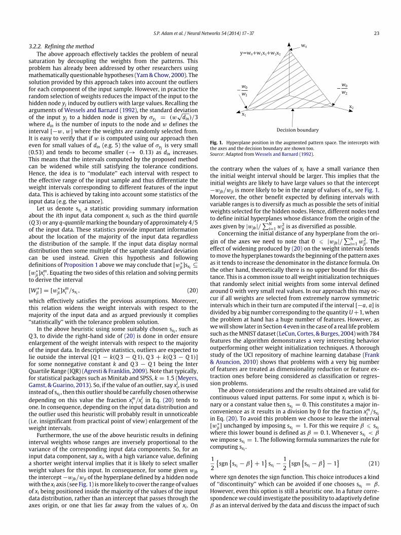
Furthermore, the use of the above heuristic results in defininginterval weights whose ranges are inversely proportional to thevariance of the corresponding input data components. So, for aninput data component, say xi, with a high variance value, defininga shorter weight interval implies that it is likely to select smallerweight values for this input. In consequence, for some given wjbthe intercept−wjb/wji of the hyperplane defined by a hidden nodewith the xi axis (see Fig. 1) ismore likely to cover the range of valuesof xi being positioned inside the majority of the values of the inputdata distribution, rather than an intercept that passes through theaxes origin, or one that lies far away from the values of xi. On

Fig. 1. Hyperplane position in the augmented pattern space. The intercepts withthe axes and the decision boundary are shown too.Source: Adapted fromWessels and Barnard (1992).

the contrary when the values of xi have a small variance thenthe initial weight interval should be larger. This implies that theinitial weights are likely to have large values so that the intercept−wjb/wji is more likely to be in the range of values of xi, see Fig. 1.Moreover, the other benefit expected by defining intervals withvariable ranges is to diversify as much as possible the sets of initialweights selected for the hidden nodes. Hence, different nodes tendto define initial hyperplanes whose distance from the origin of theaxes given by |wjb|/

Ni=1 w2

ji is as diversified as possible.Concerning the initial distance of any hyperplane from the ori-

gin of the axes we need to note that 0 6 |wjb|/N

i=1 w2ji . The

effect of widening produced by (20) on the weight intervals tendstomove the hyperplanes towards the beginning of the pattern axesas it tends to increase the denominator in the distance formula. Onthe other hand, theoretically there is no upper bound for this dis-tance. This is a common issue to all weight initialization techniquesthat randomly select initial weights from some interval definedaround 0 with very small real values. In our approach this may oc-cur if all weights are selected from extremely narrow symmetricintervals which in their turn are computed if the interval [−a, a] isdivided by a big number corresponding to the quantityU+1,whenthe problem at hand has a huge number of features. However, aswewill show later in Section 4 even in the case of a real life problemsuch as theMNIST dataset (LeCun, Cortes, & Burges, 2004)with 784features the algorithm demonstrates a very interesting behavioroutperforming other weight initialization techniques. A thoroughstudy of the UCI repository of machine learning database (Frank& Asuncion, 2010) shows that problems with a very big numberof features are treated as dimensionality reduction or feature ex-traction ones before being considered as classification or regres-sion problems.

The above considerations and the results obtained are valid forcontinuous valued input patterns. For some input xi which is bi-nary or a constant value then sxi = 0. This constitutes a major in-convenience as it results in a division by 0 for the fraction xmi /sxiin Eq. (20). To avoid this problem we choose to leave the interval[w∗

ji] unchanged by imposing sxi = 1. For this we require β 6 sxiwhere this lower bound is defined as β = 0.1. Whenever sxi < βwe impose sxi = 1. The following formula summarizes the rule forcomputing sxi .

12

sgn

sxi − β

+ 1

sxi −

12

sgn

sxi − β

− 1

(21)

where sgn denotes the sign function. This choice introduces a kindof ‘‘discontinuity’’ which can be avoided if one chooses sxi = β .However, even this option is still a heuristic one. In a future corre-spondencewe could investigate the possibility to adaptively defineβ as an interval derived by the data and discuss the impact of such


a formulae on specific experiments. In the present research thebenchmarks and realworld problems tackled provide no hints as towhich is the optimum formula for sxi definition in this specific case.

Typically, normalization or scaling is applied (Bishop, 1995) sothat the input samples are in the interval [−1, 1],mainly in order tofacilitate training (LeCun, 1993). These operations normally do notalter the status of the input data. So, the previous considerationsremain valid and the use of the term sxi for properly modulatingthe original weight intervals [w∗

ji] still applies after normalizationor scaling of the input data. For the rest of this paper, we assumethat the values of the input patterns are normalized to be in theinterval [−1, 1] or the interval [0, 1]. Under these hypotheses wemay state that the relation [w∗

ji]sxi ⊆ [w∗

ji]1 is valid and suggeststhat solving the following equations:Wjisxi = [w∗

ji], 1 6 i 6 N (22)

permits to define the intervals,W ∗

ji

= [w∗

ji]1sxi

, 1 6 i 6 N (23)

that obviously satisfy the relation,

[W ∗

j1]sx1 + [W ∗

j2]sx2 + · · · + [W ∗

jN ]sxN + [w∗

jb]1

= [w∗

j1] + [w∗

j2] + · · · + [w∗

jN ] + [w∗

jb]

= [a]. (24)

Hence, the interval vector W∗j = ([W ∗

j1], [W∗

j2], . . . , [W∗

jN ], [w∗

jb])⊤

is a solution in the tolerance solution set of the interval system (S2).Recall that sxi is computed using formula (21).

3.2.3. Initializing hidden-to-hidden and hidden-to-output layer con-nection weights

The analysis presented above focuses on effective initializationof weights of the input-to-hidden layer connections. Earlier im-plementations of a complete algorithm were based on minimalassumptions regarding the initial values of weights for hidden-to-hidden and hidden-to-output layer connections, that is, ran-dom selection of values in the interval [−1, 1]. This choice gaverather satisfactory results in the case of small sized networks anddatasets, see Section 4, Suites 1 and 2 of experiments. In order todefine a full scale algorithm for initializing weights of anyMLP twoissues are considered here. The first deals with saturation of thenodes in any hidden layer, while the second defines an order ofmagnitude for the weights of connections leading to output layernodes.

In order to avoid saturation of any node in the kth hidden layerwe adopt the hypotheses of the previous analysis. This means thatweights of connections linking a node in the hidden layer k withthe outputs of nodes in the layer k − 1 are randomly selected inthe interval [−ak/(Hk−1 + 1), ak/(Hk−1 + 1)], where Hk−1 is thenumber of nodes of the layer k− 1 and ak is the active range of theactivation function of the node in the hidden layer k. The previousformula for nodes in the hidden layer k is derived considering thatthe outputs of the layer k− 1 have a maximum value equal to 1. Inpractice, instead of (Hk−1+1) the value ofHk−1 can be usedwithoutany difference regarding the training performance.

For the weights of the hidden-to-output connections differentapproaches are proposed by different researchers (Section 3.1). Inorder to optimize the choice of these weights we used the formula[−3A/

√din, 3A/

√din] introduced in Wessels and Barnard (1992)

where instead of din we setH for the number of hidden layer nodes.The authors in that paper determined the value of the scale fac-tor A = 1 through experiments with small sized networks. Weadopted the same approach but we also experimented with net-works with a higher number of nodes in the hidden layer. For

these networks when A = 1 the fraction 3A/√H becomes too

small yielding extremely narrow weight intervals for the hidden-to-output layer connections which slow the training process. Bygradually increasing the value of A we observed that the networkperformance improved and so we came up with the following ruleof thump.

The value of A = 1 is valid for networks with a relatively smallnumber of nodes in the hidden layer i.e. H / 30. For medium tolarger sized networks i.e. H > 30 the best network performancewas observed when A > 1. Experimented with H = 36 we foundthat A ≈ 1.2 and A ≈ 3 for H = 300. Finally, for H = 650 we no-ticed thatA should be set to 4 for nodeswith the logistic sigmoid ac-tivation function while for nodes with the hyperbolic tangent thisvalue should be A ≈ 2. We cannot guarantee that these results areoptimal for every considered dataset. However, the resulting inter-vals roughly confirm the findings for the weight intervals reportedin Nguyen and Widrow (1990) and Thimm and Fiesler (1994). Tothe best of our knowledge there is no specific study on this matterin the literature and in light of these results this should constitutean interesting point for deeper investigation.

3.3. Algorithm and discussion

3.3.1. Algorithm descriptionThe algorithm implementing the above approach computes one

specific interval [W ∗

ji ] for each component i of the input data aswell as the interval [w∗

jb] for the threshold. Thus, n+1 intervals arecomputed once and they are used for selecting the weights of anynode in the hidden layer.

Input data coding

1. Continuous input data are scaled to be in the interval [−1, 1](or [0, 1]). Binary variables are set to {−1, 1} (or {0, 1}).

2. For each continuous valued input data variable xi computethe third quartile Q3 and set sxi = Q3. If xi displays normaldistribution compute the sample standard deviation σxi and setsxi = 2σxi . If xi can be approximated by the normal distributionthen sxi = kσxi for some suitably chosen k. If xi is not continuousthen Apply rule (21) above.

3. Define the value of the parameter a for the bounds of the activeregion interval [−a, a] depending on the type of the activationfunction of the jth node, see Section 3.3.2 hereafter.

Computing weights of input to hidden layer connections

4. For each node j in the hidden layer and any input connection ithe weight wji is randomly selected with uniform distributionfrom the interval [W ∗

ji ] defined using relation (23) above.5. For each node j in the hidden layer the weight wjb of the bias is

randomly selected with uniform distribution from the interval[w∗

jb] defined using relation (19) above.

Computingweights of connections from hidden layer (k−1) to hiddenlayer (k)

6. These weights are random numbers selected to be uniformlydistributed in the interval [−ak/Hk−1, ak/Hk−1] as defined in theprevious subsection.

Computing weights of hidden to output layer connections

7. Weights of the hidden to the output layer connections arerandom numbers selected to be uniformly distributed in theinterval

−3A/

√N, 3A/

√Nwhere the scale factor A is defined

in the previous subsection.


3.3.2. DiscussionStep3 of the algorithm requires setting the bounds of [−a, a] for

the active region of the sigmoid activation function. This intervalis assumed to be the region where the derivative of the sigmoidactivation function is greater than or equal to 0.04Dmax or 0.05Dmaxwhere Dmax denotes the maximum magnitude of the derivativeof the sigmoid, (Yam & Chow, 2000, 2001). For example in case alogistic sigmoid activation function is used then a = 4.59 or a =

4.34. For the experiments shown in this paper the values adoptedare those defined by the Neural Network Toolbox of MATLAB, thatis, a = 4 for the logistic sigmoid and a = 2 for the hyperbolictangent. These values are computed for λ = 1 where λ is the slopeparameter of the sigmoid activation function.

Most of the issues pertaining the formulation of the LIT-Approach were analyzed and resolved in earlier subsections. Herewe will briefly refer to the ability of the proposed method to copewith prematurely saturated units and symmetry breaking. Thesematters are reported in the literature (Hassoun, 1995; Haykin,1999) as troubles of neural network training that need to beaddressed by weight initialization. Regarding premature saturationof the units the proposed method by default defines initial weightswhich prevent saturation of the hidden nodes at an early stage oftraining. In addition, symmetry breaking that is preventing nodesfrom adopting similar functions is addressed using randomweightselection from intervals with different bounds.

Besides these matters, Wessels and Barnard (1992) note thatanother problem is what they call false local minima for which theyname three possible causes. These are the following: Stray hiddennodes, that is nodes defining initial decision boundarieswhich havebeenmoved out of the region of the sample patterns. Hidden nodeshaving duplicating function are the nodes that define separatinghyperplanes having the same initial position and orientation. Fi-nally, dead regions in the pattern space are created when in theseregions the hidden nodes are arranged so that they all happen tobe inactive, that is, there are no hyperplanes defined by the hiddennodes inside these regions. The LIT-Approach tackles these issuesbased on theway it defines theweight intervals. The issues regard-ing stray hidden nodes and dead regions are sufficiently addressedbased on the way the LIT-Approach defines the initial weight in-tervals and then on the way the hidden nodes define the initialhyperplanes to be in the heart of the pattern data, see Section 3.2.2.Moreover, hidden nodes are not likely to have duplicating functiondue to the random weight selection. The LIT-Approach, while notspecifically designed to tackle these specific problems, it, however,addresses them efficiently as shown by the results of the exper-iments hereafter. Based on the advantages of distributions suchas those proposed in Sonoda and Murata (2013) there might beimprovements concerning how the LIT-Approach tackles randomweight selection, now defined by uniform distribution.

Finally, we need to note that the proposed approach does notintend to deal with the problem of structural local minima inthe weight space. This issue concerns the training phase of anMLP and it has effectively been tackled in Magoulas, Vrahatis, andAndroulakis (1997).

4. Experimental evaluation

In order to assess the effectiveness of the proposed methodwe designed and conducted three different suites of experiments.The first suite deals with the comparison of the performance ofthe proposed method against six different weight initializationmethods which are based on random selection of initial weightsfrom predefined intervals. The benchmarks used for this first suitemainly concern classification problems, while one of them dealswith regression and a secondwith prediction of a highly non-linearphenomenon. Moreover, a number of experiments were executed

on function approximation and they are presented in a separatesubsection. The second suite constitutes a thorough comparisonof the proposed LIT-Approach with the well known initializationprocedure proposed by Nguyen and Widrow (1990).

The performance measures considered for all experiments are:the convergence success of the training algorithm, the conver-gence rate and the generalization performance achieved for thetest patterns. The convergence success of the training algorithmis the number of initial weight sets for which the training algo-rithm reached the predefined convergence criteria. The conver-gence rate is the number of epochs needed for the training toconverge. For benchmarks with continuous valued output, gener-alization performance is computed using the mean absolute errorof the output of the network and the target output, and for classifi-cation benchmarks, generalization is defined as the percentage ofsuccessfully classified previously unknown test patterns. The anal-ysis of the experimental resultswas carried out using the statisticalanalysis package SPSS v17.0 (Green & Salkind, 2003), STATService2.0 (Parejo, García, Ruiz-Cortés, & Riquelme, 2012) and the R sta-tistical computing environment.

Hereafter, training a network for some specific benchmarkwithinitial weights selected using some weight initialization method iscalled a trial. A training experiment is a set of trials correspondingto training the network for some specific benchmark using a set ofinitial weights selected by the same weight initialization method.

4.1. Suite 1 of experiments

4.1.1. Experimental setupThis suite of experiments was set up in order to investigate the

efficiency of the proposed approach on a relatively broad spectrumof real world problems. Comparison is done against the follow-ing (in alphabetical order of the abbreviations used) well knownweight initialization methods; BoersK, (Boers & Kuiper, 1992),Bottou, (Bottou, 1988), Kim–Ra, (Kim & Ra, 1991), NW, (Nguyen& Widrow, 1990), SCAWI, (Drago & Ridella, 1992), and Smieja,(Smieja, 1991).

The real world problems adopted for the experiments arebenchmarks reported in various research papers used to compareperformance of different weight initialization methods, as forexample Fernández-Redondo and Hernández-Espinosa (2001),Thimm and Fiesler (1997), Yam and Chow (2000, 2001). These realworld problems are briefly described in the following paragraph.Detailed description andmore information can de found in the UCIrepository of machine learning database (Frank & Asuncion, 2010)and references cited therein.

1. Auto-MPG prediction (inputs:7, outputs:1). This dataset con-cerns city-cycle fuel consumption inmiles per gallon, to be pre-dicted in terms of 3 multi-valued discrete and 4 continuousattributes. The number of instances is 398. Six patterns withmissing values have been removed.

2. British language vowels recognition (inputs:10, outputs:11).As stated in the benchmark summary, this is a speaker inde-pendent recognition problem of the eleven steady state vow-els of British English using a specified training set of 10 linearprediction coefficients derived log area ratios. The originaldataset comprises 991 instances pronounced by differentspeakers. A subset containing the first 330 instances were re-tained for training and testing.

3. Glass identification (inputs:9, outputs:1). Based on 9 attributes,this classification of types of glass was motivated by crimino-logical investigation. The dataset used is the glass2 download-able from PROBEN1 (1994) ftp site. It consists of 214 instancesalready preprocessed and so there are no missing values.


Table 1Architectures of networks and training parameters used for Suite 1 of the experiments.

Benchmark Network architecture Activation functiona Learning rate Convergence criterion Max cycles Input data scale

Auto-MPG 7-3-1 logsig 0.3 0.01 500 [−1, 1]British vowels 10-20-11 tansig 0.05 90% 800 [−1, 1]

Glass 9-10-8-6 logsig 0.6 0.04 800 [0, 1]Servo 12-3-1 logsig 0.1 0.008 500 [−1, 1]Solar 12-5-1 logsig 0.3 0.005 500 [0, 1]Wine 13-6-3 tansig 0.2 95% 500 [−1, 1]

a logsig denotes the logistic sigmoid function and tansig is the hyperbolic tangent.

Table 2Convergence success results in 100 trials for Suite 1 of the experiments.

Benchmark Initialization algorithmsBoersK Bottou Kim–Ra LIT-A NW SCAWI Smieja

Auto-MPG 100 100 100 100 100 100 100British vowels 91 100 100 100 91 100 100

Glass 22 21 0 72 12 0 0Servo 100 100 100 100 99 100 100Solar 100 100 100 100 92 100 100Wine 100 100 100 100 100 100 100

4. Servo prediction (inputs:12, outputs:1). Originally this bench-mark was created by Karl Ulrich (MIT) in 1986 and refers to ahighly non-linear phenomenon that is predicting the rise timeof a servomechanism in terms of two (continuous) gain settingsand two (discrete) choices of mechanical linkages. The datasetconsists of 167 patterns and has no missing values.

5. Solar sunspot prediction (inputs:12, outputs:1). The datasetcontains the sunspot activity for the years 1700 to 1990. Thetask is to predict the sun spot activity for one of those yearsgiven the activity of the preceding twelve years. A total of 279different patterns are derived from the raw data.

6. Wine classification (inputs:13, outputs:3). These data are theresults of a chemical analysis of wines grown in the same regionin Italy but derived from three different cultivars. The analysisdetermined the quantities of 13 constituents found in each ofthe three types ofwines. The dataset contains 178 instances andhas no missing values.

The original datasets were preprocessed to eliminate duplicatepatterns and values were scaled to match requirements set by theweight selection procedures. These operationswere performed ac-cording to PROBEN1 guidelines, (Prechelt, 1994). Unless otherwisestated, the datasetswere partitioned to training sets using approxi-mately 75% of the patterns and to test sets using the remaining 25%.For the Servo prediction benchmark the training set was made us-ing 84 patterns and the test set using 83 patterns. The training andthe test sets are defined once and used for all experiments. Duringnetwork training the patterns of the training set are presented inthe same order using the trains i.e. the online sequential trainingprocedure of MATLAB.

A total number of 42 experiments were set up for these 6 prob-lems and the 7weight initializationmethods. Each experimentwascarried out using a set of 100 initial weight vectors, selected bythe corresponding method. The same network architecture wasinitialized with these vectors and trained using online BP. Thenetwork architecture and the training parameters, used in thisarrangement, are reported in Table 1. These parameters are sim-ilar to those found by Thimm and Fiesler (1994).(a) Learning rate is the rate used by the vanilla BP online algorithm.(b) Convergence criterion is either the goal set for the minimiza-

tion of the error function or the minimum percentage of thetraining patterns correctly classified by the network.

(c) Max cycles denote the maximum number of BP cycles. Duringa cycle all training patterns are presented to the network inrandom order and weights are updated after every trainingpattern. Training stops when Max cycles number is reached.

(d) Input data scale indicates the interval used by all weight ini-tialization algorithms except the Nguyen–Widrow algorithm,which scales input data values in the interval [−1, 1].

4.1.2. Analysis of the resultsTables 2–4 report the experimental results on the benchmarks

considered for the aforementioned performancemeasures. A quicklook at these results shows that the proposed approach improvesnetwork performance for all parameters.

The comparison of the efficiency of the different initializationmethods is based on the statistical analysis of the results obtained.In order to evaluate the statistical significance of the observed per-formance one-way ANOVA (Green & Salkind, 2003) was used totest equality of means. ANOVA relies on three assumptions: inde-pendence, normality and homogeneity of variances of the samples.This procedure is robustwith respect to violations of these assump-tions except in the case of unequal variances with unequal samplesizes, which is true for the Glass benchmark as the larger group sizeis more than 1.5 times the size of the smaller group.

The validity of the normality assumption is omitted and Lev-ene’s test for testing equality of variances is conducted, (Ra-machandran & Tsokos, 2009). Homogeneity of variances is rejectedfor all cases by Levene’s test and so Tamhane’s post-hoc proce-dure, Ramachandran and Tsokos (2009), is applied to performmul-tiple comparisons analysis of the samples. The significance levelset for these tests is α = 0.05. The p-value (Sig.) indicated foreach initialization method, concerns comparison with the pro-posed method and the mean value is marked with an ∗ whenequality of means is rejected p-value <0.05. The analysis of theGlass benchmark results was performed pairwise between suc-cessful initialization methods using the Mann–Whitney test.

Table 5 reports for each initialization method how manytimes a method delivers superior, equal or inferior performancewhen compared (pairwise comparisons) with all other methodsregarding convergence rate and generalization. The advantageoffered by the proposed method to achieve better convergencerate is manifested by these results. So, performance of a neuralnetworkwhenweights are initializedwith the proposedmethod issuperior in 42% of the cases. In 50% of the cases performance is thesame with all other methods and only in 6% the proposed methoddelivers inferior performance to the training algorithm.

In terms of generalization the proposed method though havingamarginally better scorewhen compared to themethodof KimandRaproves to be better than all the othermethods in all benchmarks,


Table 3Convergence rate results for Suite 1 of the experiments.

Benchmarks Initialization algorithmsLIT-A BoersK Bottou Kim–Ra NW SCAWI Smieja

Auto-MPGMean 2.19 2.51 2.38 2.97* 4.73* 2.34 2.26St.D. 0.46 1.03 0.86 0.39 2.88 0.59 0.52Sig. 0.106 0.690 0.000 0.000 0.638 1.000

British vowelsMean 471.29 521.88* 476.99 487.96 517.77* 468.83 476.58St.D. 41.59 94.16 46.15 36.50 79.28 54.82 53.82Sig. 0.000 1.000 0.060 0.000 1.000 1.000

ServoMean 88.07 87.31 86.37 124.07* 77.17 96.02* 86.88St.D. 8.66 14.75 12.87 3.14 35.29 9.02 8.96Sig. 1.000 0.999 0.000 0.071 0.000 1.000

SolarMean 142.67 150.26 159.74* 169.88* 233.05* 160.15* 158.08*

St.D. 30.73 28.66 30.90 18.33 91.24 29.87 29.74Sig. 0.794 0.003 0.000 0.000 0.001 0.008

WineMean 11.42 10.57* 10.73* 11.65 10.50 11.08 11.26St.D. 1.10 1.68 1.42 0.98 5.49 1.32 1.52Sig. 0.001 0.004 0.932 0.899 0.658 1.000

Glass

Min 600 616 660 a 563 a a

Max 799 785 795 a 789 a a

Median 721.00 730.50 759.00* a 718.00 a a

Sig. 0.214 0.001 a 0.975 a a

* denotes that the mean value of the initialization method is significantly different from the mean value of LIT-A using the indicated p-values (Sig.) computed by thepost-hoc analysis of the ANOVA results.

a The initialization method failed to meet the convergence criteria exceeding the maximum number of cycles in all trials.

Table 4Generalization performance results for Suite 1 of the experiments.

Benchmarks Initialization algorithmsLIT-A BoersK Bottou Kim–Ra NW SCAWI Smieja

Auto-MPGMean 0.0743 0.0750 0.0748 0.0738 0.0778* 0.0739 0.0741St.D. 0.0041 0.0052 0.0047 0.0018 0.0073 0.0043 0.0041Sig. 0.999 1.000 1.000 0.001 1.000 1.000

British vowelsMean 96.23% 93.72%* 96.29% 96.27% 94.52%* 95.86% 96.18%St.D. 1.60% 2.85% 1.37% 1.18% 2.70% 1.81% 1.45%Sig. 0.000 1.000 1.000 0.000 0.933 1.000

ServoMean 0.0792 0.0854* 0.0839* 0.0797* 0.0969* 0.0842* 0.0801*

St.D. 0.0010 0.0055 0.0045 0.0002 0.0145 0.0049 0.0020Sig. 0.000 0.000 0.000 0.000 0.000 0.002

SolarMean 0.0924 0.0924 0.0919 0.0876* 0.1025* 0.0911 0.0917St.D. 0.0040 0.0030 0.0030 0.0019 0.0107 0.0029 0.0034Sig. 1.000 0.999 0.000 0.000 0.160 0.980

WineMean 99.84% 98.98%* 99.38%* 99.80% 98.69%* 99.58% 99.40%*

St.D. 0.57% 1.20% 1.05% 0.64% 1.48% 0.93% 1.22%Sig. 0.000 0.003 1.000 0.000 0.282 0.025

Glass

Min 59.62% 67.31% 65.38% a 65.38% a a

Max 71.15% 75.00% 75.00% a 75.00% a a

Median 65.38% 71.15%* 69.32%* a 69.23%* a a

Sig. 0.000 0.000 a 0.000 a a


a The initialization method failed to meet the convergence criteria exceeding the maximum number of cycles in all trials.

Table 5Summary of pairwise comparisons score for each method for Suite 1 of the experiments.

Initialization method Convergence rate GeneralizationSuperior Equal Inferior Superior Equal Inferior

BoersK 12 19 5 6 17 13Bottou 12 20 4 10 20 6Kim–Ra 4 12 20 16 15 5LIT-A 15 19 2 17 15 4NW 6 13 17 4 5 27

SCAWI 7 20 9 8 20 8Smieja 8 24 4 9 20 7

except in the case of the Glass benchmark, see Table 4. For the Glassbenchmark the generalization performance seems to be betterfor the methods of Boers–Kuiper, Bottou and Nguyen–Widrowcompared to our LIT-Amethod. However, one should also take into

account the number of successful experiments for each method.Generalization ‘‘achieved’’ by the proposed method is superior in47% of the cases, while in 42% of the cases performance is the samewith other methods and only in 11% of the cases the proposed


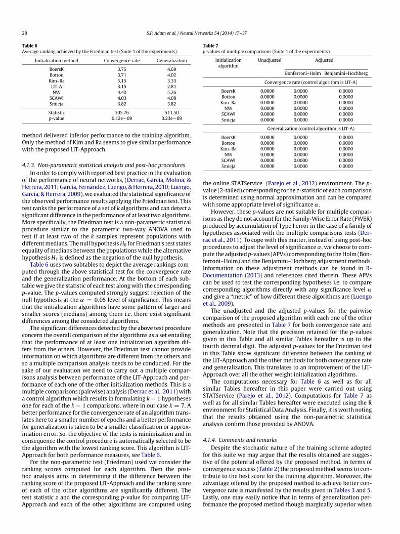
Table 6Average ranking achieved by the Friedman test (Suite 1 of the experiments).

Initialization method Convergence rate Generalization

BoersK 3.75 4.69Bottou 3.71 4.02Kim–Ra 5.15 3.33LIT-A 3.15 2.81NW 4.40 5.26

SCAWI 4.03 4.08Smieja 3.82 3.82

Statistic 305.76 511.50p-value 0.12e−09 0.23e−09

method delivered inferior performance to the training algorithm.Only the method of Kim and Ra seems to give similar performancewith the proposed LIT-Approach.

4.1.3. Non-parametric statistical analysis and post-hoc proceduresIn order to complywith reported best practice in the evaluation

of the performance of neural networks, (Derrac, García, Molina, &Herrera, 2011;García, Fernández, Luengo, &Herrera, 2010; Luengo,García, &Herrera, 2009),we evaluated the statistical significance ofthe observed performance results applying the Friedman test. Thistest ranks the performance of a set of k algorithms and can detect asignificant difference in the performance of at least two algorithms.More specifically, the Friedman test is a non-parametric statisticalprocedure similar to the parametric two-way ANOVA used totest if at least two of the k samples represent populations withdifferentmedians. The null hypothesisH0 for Friedman‘s test statesequality of medians between the populations while the alternativehypothesis H1 is defined as the negation of the null hypothesis.

Table 6 uses two subtables to depict the average rankings com-puted through the above statistical test for the convergence rateand the generalization performance. At the bottom of each sub-tablewe give the statistic of each test alongwith the correspondingp-value. The p-values computed strongly suggest rejection of thenull hypothesis at the α = 0.05 level of significance. This meansthat the initialization algorithms have some pattern of larger andsmaller scores (medians) among them i.e. there exist significantdifferences among the considered algorithms.

The significant differences detected by the above test procedureconcern the overall comparison of the algorithms as a set entailingthat the performance of at least one initialization algorithm dif-fers from the others. However, the Friedman test cannot provideinformation onwhich algorithms are different from the others andso a multiple comparison analysis needs to be conducted. For thesake of our evaluation we need to carry out a multiple compar-isons analysis between performance of the LIT-Approach and per-formance of each one of the other initialization methods. This is amultiple comparisons (pairwise) analysis (Derrac et al., 2011) witha control algorithm which results in formulating k − 1 hypothesesone for each of the k − 1 comparisons, where in our case k = 7. Abetter performance for the convergence rate of an algorithm trans-lates here to a smaller number of epochs and a better performancefor generalization is taken to be a smaller classification or approx-imation error. So, the objective of the tests is minimization and inconsequence the control procedure is automatically selected to bethe algorithmwith the lowest ranking score. This algorithm is LIT-Approach for both performance measures, see Table 6.

For the non-parametric test (Friedman) used we consider theranking scores computed for each algorithm. Then the post-hoc analysis aims in determining if the difference between theranking score of the proposed LIT-Approach and the ranking scoreof each of the other algorithms are significantly different. Thetest statistic z and the corresponding p-value for comparing LIT-Approach and each of the other algorithms are computed using

Table 7p-values of multiple comparisons (Suite 1 of the experiments).

Initializationalgorithm

Unadjusted Adjusted

Bonferroni–Holm Benjamini–Hochberg

Convergence rate (control algorithm is LIT-A)

BoersK 0.0000 0.0000 0.0000Bottou 0.0000 0.0000 0.0000Kim–Ra 0.0000 0.0000 0.0000NW 0.0000 0.0000 0.0000

SCAWI 0.0000 0.0000 0.0000Smieja 0.0000 0.0000 0.0000

Generalization (control algorithm is LIT-A)


SCAWI 0.0000 0.0000 0.0000Smieja 0.0000 0.0000 0.0000

the online STATService (Parejo et al., 2012) environment. The p-value (2-tailed) corresponding to the z-statistic of each comparisonis determined using normal approximation and can be comparedwith some appropriate level of significance α.

However, these p-values are not suitable for multiple compar-isons as they do not account for the Family-Wise Error Rate (FWER)produced by accumulation of Type I error in the case of a family ofhypotheses associated with the multiple comparisons tests (Der-rac et al., 2011). To copewith this matter, instead of using post-hocprocedures to adjust the level of significance α, we choose to com-pute the adjusted p-values (APVs) corresponding to theHolm (Bon-ferroni–Holm) and the Benjamini–Hochberg adjustment methods.Information on these adjustment methods can be found in R-Documentation (2013) and references cited therein. These APVscan be used to test the corresponding hypotheses i.e. to comparecorresponding algorithms directly with any significance level αand give a ‘‘metric’’ of how different these algorithms are (Luengoet al., 2009).

The unadjusted and the adjusted p-values for the pairwisecomparison of the proposed algorithm with each one of the othermethods are presented in Table 7 for both convergence rate andgeneralization. Note that the precision retained for the p-valuesgiven in this Table and all similar Tables hereafter is up to thefourth decimal digit. The adjusted p-values for the Friedman testin this Table show significant difference between the ranking ofthe LIT-Approach and the othermethods for both convergence rateand generalization. This translates to an improvement of the LIT-Approach over all the other weight initialization algorithms.

The computations necessary for Table 6 as well as for allsimilar Tables hereafter in this paper were carried out usingSTATService (Parejo et al., 2012). Computations for Table 7 aswell as for all similar Tables hereafter were executed using the Renvironment for Statistical Data Analysis. Finally, it is worth notingthat the results obtained using the non-parametric statisticalanalysis confirm those provided by ANOVA.

4.1.4. Comments and remarksDespite the stochastic nature of the training scheme adopted

for this suite we may argue that the results obtained are sugges-tive of the potential offered by the proposed method. In terms ofconvergence success (Table 2) the proposedmethod seems to con-tribute to the best score for the training algorithm. Moreover, theadvantage offered by the proposed method to achieve better con-vergence rate is manifested by the results given in Tables 3 and 5.Lastly, one may easily notice that in terms of generalization per-formance the proposed method though marginally superior when


Table 8Convergence success results for the function approximation benchmarks.

Benchmarks Initialization methodsBoersK Bottou Kim–Ra LIT-A NW SCAWI Smieja

Function 1 73 91 82 92 74 85 82Function 2 100 100 100 100 76 100 100Function 3 81 100 100 84 81 91 47

Table 9Convergence rate results for the function approximation benchmarks.

Benchmarks Initialization algorithmsBoersK Bottou Kim–Ra LIT-A NW SCAWI Smieja

Function 1 Mean 379.79 504.70 538.73 337.05 275.70 333.72 401.71St.D. 217.57 177.66 164.74 198.95 212.12 184.73 225.23

Function 2 Mean 6.89 6.87 8.93 6.49 69 7.23 7.36St.D. 1.61 1.54 2.25 1.40 191.28 1.95 2.34


compared, using ANOVA, to the Kim–Ra it proves to be better thanall the other methods in all benchmarks, except the Glass bench-mark, see Tables 4 and 5. These conclusions are strongly supportedby the non-parametric statistical analysis with the Friedman test.Though these results are indicative and for comparison purposes,they provide significant evidence regarding the efficiency of theproposed method.

4.2. Function approximation

4.2.1. Setup of the experimentsIn order to cover the whole range of problems for which MLPs

are used, one needs to consider the problem of approximatinganalytically defined non-linear functions. This constitutes anecessary prerequisite for a ‘‘fair’’ comparison first and foremostwith the method of Nguyen and Widrow, as these researchersinitially demonstrated their method on a function approximationproblem. The functions used as benchmarks are defined in thefollowing paragraphs.Function 1. The function for this benchmark is the one reported inthe original paper of Nguyen and Widrow (1990),

y = 0.5 sinπx21

sin(2πx2).

The network used here, is a 3-layer (2-21-1) architecture with thehyperbolic tangent activation function for the hidden layer nodesas well as for the output node. A total of 625 (=25 × 25) pointsare randomly selected, using uniform distribution, in the interval[−1, 1] × [−1, 1]. Among these points 450 are used for trainingand 175 for testing the network.Function 2. The function considered here is a variant of the functionconsidered in Yam and Chow (2000, 2001). This function is amapping of eight input variables, taken in the interval [0, 1], intothree output ones defined by the following three equations:

y1 = (x1x2 + x3x4 + x5x6 + x7x8) /4

y2 =

(x1 + x2 + x3 + x4 + x5 + x6 + x7 + x8)/8

y3 = (1 − y1)1/3.

For this benchmark, a 8-12-3 network architecture was used withlogistic activation functions for nodes of the hidden and the outputlayer. A set of 75 patterns is formed by randomly sampling, withuniform distribution, values for the input variables and calculatingoutput values. Among these input–output patterns, 50 are used fortraining the network and25 for testing, as in YamandChow (2001).

Function 3. The function used here is a real-valued non-linearfunction of two variables, taken in the interval [−1, 1], defined bythe formula:

y = sin(2πx1x2)/(2πx1x2).

A 3-layer network architecture with 30 nodes in the hidden layerwas adopted for this benchmark. All nodes in the hidden layeras well as the output node have a hyperbolic tangent activationfunction. The training set is formed by taking 320 patterns of thetotal 400 (=20 × 20) that are randomly selected using uniformdistribution. The rest 80 patterns constitute the test set.

A total of 21 training experiments were executed for the above3 functions and the 7 (LIT-A plus other six) weight initializationmethods considered in this section. Each training experimentis made up of a hundred (100) initial weight vectors derivedusing one of the weight initialization methods. Networks in allexperiments are trained using the Levenberg–Marquardt method(LM), (Hagan, Demuth, & Beale, 1996; Hagan & Menhaj, 1994;Marquardt, 1963). The performance goal for the network outputerror is set to 1.0e−04 for Functions 1 and 2, and 1.0e−03 forFunction 3. If the performance goal is not met when a maximumnumber of 1000 epochs is reached then the training stops. Thelearning rate for all experiments of Function 1 is set to 0.1 and 0.5for the other two benchmarks. Results of the training experimentsare reported in Tables 8–10 hereafter.

For the benchmarks Functions 1 and 3 LIT-A was applied us-ing 1.5σxi for the term sxi . This choice is based on the assumptionthat the input data are approximately normally distributed, andtherefore sxi in the LIT-Approach was ‘‘roughly’’ approximated us-ing 1.5σxi instead of the third quartile Q3.

4.2.2. Analysis of the resultsThe results obtained regarding the performance measures set

are shown in Tables 8–10. A rough observation of these resultsshows that the proposed LIT-Approach remains on top of theother methods as in the previous Suite 1 concerning convergencerate (Table 9) while being among the best methods regardingconvergence success (Table 8) and generalization (Table 10).

Comparison between the performance of the different initial-ization methods, for the function mapping experiments, is carriedout using the non-parametric Friedman test. The average rankingscomputed are reported in Table 11. The hypotheses of the Fried-man test and the post-hoc procedures performed are the same asthose for Suite 1 of the experiments. The unadjusted and the ad-justed p-values of the post-hoc procedures are given in Table 12.The fact that the control procedure for the convergence rate is LIT-Approach together with the p-values in Table 12underline the su-


Table 10Generalization performance results for the function approximation benchmarks.

Benchmarks Initialization algorithmsBoersK Bottou Kim–Ra LIT-A NW SCAWI Smieja




Table 11Average ranking achieved by the Friedman test (function approximation bench-marks).


BoersK 3.87 3.60Bottou 3.59 3.24Kim–Ra 4.91 3.80LIT-A 2.99 3.25NW 4.57 6.43

SCAWI 3.45 3.48Smieja 4.61 4.20

Statistic 195.05 486.06p-value 0.10e−09 0.21e−09

Table 12p-values of multiple comparisons (function approximation benchmarks).


Unadjusted Adjusted




SCAWI 0.0091 0.0182 0.0106Smieja 0.0000 0.0000 0.0000

Generalization (control algorithm is Bottou)

BoersK 0.0394 0.1586 0.0690Kim–Ra 0.0015 0.0073 0.0034LIT-A 0.9397 1.0000 1.0000NW 0.0000 0.0000 0.0000

SCAWI 0.1706 0.5119 0.2389Smieja 0.0000 0.0000 0.0000

periority of the proposedmethod. On the other hand the algorithmof Bottou is considered to be the control procedure for the general-ization. This does not prove that Bottou’s method performs betterthan LIT-Approach as the corresponding unadjusted and adjustedp-values denote that the performance of these algorithms is thesame.

4.2.3. Comments and remarksIn termsof convergence success (Table 8) all initializationmeth-

ods seem to have similar performance while the method of Bottougives the best results as the networks initialized with this methodare trapped in local minima for only 9 trials (2% of the total num-ber of trials). The results reported in Table 9 support the improve-ment in convergence rate offered by the proposed method, whencompared with other weight initialization methods in the contextof these function approximation problems. Concerning generaliza-tion, results in Table 10 indicate that the performance observed forthe LIT-Approach seems to be among the best of all methods. Theseremarks are confirmed by the results of the Friedman test in Ta-ble 11 and the post-hoc procedures in 12, especially regarding theconvergence rate.

On the other hand generalization performance of the LIT-Approach is found to be marginally weaker than the performanceof Bottou’s method. Compared with the results of Suite 1 perfor-mance of the LIT-Approach in terms of generalization is consideredhere suboptimal. Various reasons may account for this. One reasonis the fact that the distribution of the input data for benchmarksFunctions 1 and 3 was considered to be the normal and there-fore it was ‘‘roughly’’ approximated using the term 1.5σxi . Actu-ally, it seems that defining weight intervals with different rangesfor the input variables seemsmeaningless for function approxima-tion problems as these are different from classification ones. More-over, speaking about outliers and extreme input data in the case ofa function approximation benchmark is useless. However, in thecontext of the LIT-Approach we have not considered that functionapproximation should be treated as a special case. So, it remains asan open issue for further investigation, in the case of function ap-proximation, the estimation of the optimal value k for the term kσxi ,given a specific function approximation problem. However, theseclaims, as well as others, need to be further investigatedwithmorebenchmarks together with taking into account the whole input setof training patterns.

What is noteworthy here is the poor generalization per-formance achieved by the network when initialized with theNguyen–Widrowmethod; in this case, it is very likely that the net-work gets trapped in local minima. One should note that, seem-ingly, the Nguyen–Widrow method showed notable performancein convergence ratewhen experimentingwith the non-linear Func-tion 1, which is reported in the original paper by Nguyen andWidrow (Nguyen &Widrow, 1990).


4.3.1. Experimental setupSetting up this suite is motivated by the importance the re-

search community has devoted to theweight initializationmethodof Nguyen and Widrow. In addition, popular neural networkpackages, such as the Neural Network Toolbox of MATLAB andthe Encog Neural Network Framework (2013), use this techniqueas the default initialization algorithm for neural networks.

The datasets used for these experiments and basic featuresof the problems are briefly outlined here. More details on thesebenchmarks can be found in theUCI repository ofmachine learningdatabase (Frank & Asuncion, 2010) and references cited therein.

1. Iris classification benchmark (inputs:4, outputs:3). This bench-mark is known as Fisher’s Iris problem. Based on the values ofsepal length and width, petal length and width, the class of irisplant needs to be predicted. The dataset contains 3 classes of 50instances each, where each class refers to a type of iris plant.The training set used consists of 120 examples and the test setof 30 examples.

2. Pima Indians Diabetes problem (inputs:8, outputs:2). The aimof this real world-classification task is to decide when a PimaIndian individual is diabetes positive or not. The values of


Table 13Architectures of networks and training parameters used for Suite 2 of experiments.

Benchmark Network architecture Activation functiona Total weights Learning rateb Max epochsc Goal for MSEc Min gradientc

Iris 4-2-3 logsig 19 0.90 5000 0.01 1.0e−09Diabetes 8-2-2-2 logsig 30 0.50 2000 0.14 1.0e−09Thyroid 21-4-3 logsig 103 0.50 2000 0.035 1.0e−09Yeast 8-16-10 logsig 314 0.50 5000 0.05 1.0e−09Gene2 120-4-2-3 tansig 503 0.50 5000 0.0075 1.0e−09

a logsig denotes the logistic sigmoid function and tansig is the hyperbolic tangent.b Learning rate is the initial learning rate used for training.c Training stops when at least one of the following conditions is satisfied, Max epochs is reached, Error of the network output becomes lower than or equal to Goal for

MSE, Min gradient is reached during training.

Table 14Convergence success results for Suite 2 of experiments.

Benchmark Training algorithmsAGDM BFGS LM RBP SCG

NW LIT-A NW LIT-A NW LIT-A NW LIT-A NW LIT-AIris 18.2 100.0 11.5 46.3 42.8 96.0 76.1 99.9 46.9 98.5

Diabetes 12.2 77.2 21.5 73.9 40.3 63.4 39.1 77.3 40.5 70.2Thyroid 19.0 99.1 58.1 73.9 85.2 99.9 100.0 100.0 93.6 91.3Yeast 94.5 100.0 35.3 98.3 68.1 94.4 100.0 100.0 84.7 100.0Gene2 20.1 86.5 1.8 6.7 32.5 43.9 6.9 35.2 26 75.7

All numbers indicated are in the range 0 · · · 100 to denote the percentage of successful training trials.

the input attributes represent personal data and result froma medical examination. The dataset consists of a total of 768patterns. The training set used consists of 576 patterns and thetest set of the 192 remaining patterns.

3. Thyroid classification problem (inputs:21, outputs:3). Based onpatient query data and patient examination data the task is todecide whether the patient’s thyroid has over function, normalfunction, or under function. Using the original thyroid1 datasetthe training set is made from 5400 patterns while the test set ismade from 1800 patterns.

4. Yeast classification problem (inputs:8, outputs:10). Yeast isa relatively complicated organism possessing different typesof proteins, related to the cytoskeletal structure of thecell, the nucleus organization, membrane transporters andmetabolic related proteins (as mitochondrial proteins). Afterthe necessary preprocessing, Yeast data is found to include 1453patterns, that is, there are 1453 proteins labeled according to10 sites. As the dataset is radically imbalanced, the training setwas generated by randomly selecting approximately the 70% ofpatterns from each of the 10 sites, giving a total of 1019 trainingpatterns. The rest of the patterns, i.e. 434, were included in thetest set.

5. Gene2 classification (inputs:120, outputs:3). This is a binaryproblem with 120 input attributes and 3 output classes. Thegoal of this classification task is to decide, from a window of60 DNA sequence elements (nucleotides), whether the middleis either an intron/exon boundary (a donor), or an exon/intronboundary (an acceptor), or none of them. The dataset forthis problem was created based on the Splice-junction GeneSequences dataset from the UCI repository, (Frank & Asuncion,2010). It consists of 2990 patterns (duplicates are excluded) andit is partitioned to form the training set (2243 patterns) and thetest set (747 patterns).

The original datasets were preprocessed to eliminate duplicatepatterns and values were scaled to match requirements setby the weight selection procedures. These operations wereperformed according to PROBEN1 guidelines, (Prechelt, 1994).Unless otherwise stated, the training sets used are made with 75%of the patterns of the initial dataset and the test sets with the rest25% of the patterns.

For each benchmark a neural network architecture was de-fined. Batch processing was used for training with five well known

training algorithms, namely, the Adaptive gradient descent withmomentum (AGDM) (Hagan et al., 1996; Vogl, Mangis, Rigler,Zink, & Alkon, 1988), Resilient back-propagation (RBP) (Ried-miller &Braun, 1993), the Levenberg–Marquardtmethod (LM) (Ha-gan et al., 1996; Hagan & Menhaj, 1994; Marquardt, 1963),Scaled conjugate gradient (SCG) (Moller, 1993) and the Broy-den–Fletcher–Goldfarb–Shanno method (BFGS) (Gill, Murray, &Wright, 1981). For each benchmark a set of a thousand (1000)initial weight vectors was created by each one of the two initializa-tionmethods and used in all experiments. A total of 50 (=5 bench-marks × 5 training algorithms × 2 initialization methods) exper-iments were carried out, giving a total of 25000 weights for eachinitialization method. Architectures of the networks and trainingparameters used are those reported in the literature (Anastasiadis,2005) to be the most appropriate for each problem; see Table 13.Note that the value of themomentum coefficientwas set to 0.5 andall networks are fully connected without intra-layer or supra-layerconnections.

4.3.2. Analysis of the resultsThe results obtained regarding the performance measures set

are shown in Tables 14–16. A rough observation of these resultsshows that the proposed LIT-Approach delivers successful networkperformance for all parameters.

The statistical analysis, applied on results in Tables 15 and 16,concerns the comparison of the two initialization techniques us-ing t-test for independent unpaired samples data. However, whilethe samples are independent by default, application of the t-testassumes that these samples are drawn from normally distributedpopulations with equal variances. The Shapiro–Wilk test (Shapiro& Wilk, 1965) was used to test the normality assumption, withα = 0.05, while SPSS automatically uses Levene’s test for equal-ity of variances, (Green & Salkind, 2003). In all experiments, ex-cept one (training Gene2 benchmark with the BFGS algorithm forgeneralization performance) the hypothesis of normality is re-jected (p-value <0.05) for the results of both weight initializationmethods and so the non-parametric Mann–Whitney test for inde-pendent samples is used to compare equality of medians. The sta-tistical significance of the comparison, that is the p-value (Sig.) in-dicated underneath the results for every pair of experiments, is theone calculated by the Mann–Whitney test (or the t-test, when thenormality assumption is validated), (Green & Salkind, 2003).


Table 15Convergence rate results for Suite 2 of experiments.

Training algorithmsAGDM BFGS LM RBP SCG

NW LIT-A NW LIT-A NW LIT-A NW LIT-A NW LIT-AIris

Min 174 111 9 21 4 3 91 33 15 14Max 4927 143 1076 3272 3532 621 4027 1381 4508 205

Median 981 117 59 51 13 7 512 67 167 26Sig. 0.000 0.863 0.000 0.000 0.000

DiabetesMin 254 366 63 56 6 5 67 74 59 48Max 1996 1999 1935 1835 1925 1903 1977 1996 1993 1971

Median 1021 1436 250 123 27 18 465 681 390 166Sig. 0.000 0.000 0.000 0.000 0.000

ThyroidMin 282 211 186 176 10 10 92 84 570 329Max 1992 528 1976 1971 1999 1659 1455 687 1991 1980

Median 402 319 788.5 575 45 25 268 103 1229 732.5Sig. 0.000 0.000 0.000 0.000 0.000

YeastMin 729 906 168 187 7 7 74 73 102 103Max 4753 1594 4636 4348 4560 4432 280 197 4701 800

Median 1553 1148.5 403 423 20 12 130 112.5 196 145Sig. 0.000 0.534 0.000 0.000 0.000

Gene2Min 489 283 110 57 12 11 436 222 129 61Max 4971 4956 4757 4990 4976 4675 4946 4654 4974 4962

Median 2426 720 1936 794 31 24 2281 697.5 1118 155Sig. 0.000 0.016 0.000 0.000 0.000

Table 16Generalization performance resultsa for Suite 2 of experiments.

Training algorithmsAGDM BFGS LM RBP SCG

NW LIT-A NW LIT-A NW LIT-A NW LIT-A NW LIT-AIris

Min 95.56 95.56 91.11 91.11 91.11 91.11 93.33 93.33 91.11 93.33Max 97.78 97.78 97.78 97.78 97.78 97.78 97.78 97.78 97.78 97.78

Median 95.56 95.56 95.56 95.56 95.56 95.56 95.56 95.56 95.56 97.78Sig. 0.000 0.000 0.000 0.351 0.000

DiabetesMin 70.83 69.27 68.23 65.63 68.75 67.71 68.23 68.23 68.75 68.23Max 78.65 78.65 80.73 79.17 79.69 79.17 79.17 79.17 79.69 80.21

Median 75.52 76.04 75.52 75.52 75.52 75.00 75.00 75.52 75.52 75.52Sig. 0.000 0.029 0.011 0.000 0.234

ThyroidMin 92.28 93.78 92.22 92.50 92.10 92.18 92.25 93.05 97.11 96.67Max 94.22 94.17 98.28 98.50 99.00 99.00 98.30 98.75 98.33 98.44

Median 93.67 94.06 97.44 97.78 98.28 98.33 97.07 97.90 97.83 97.86Sig. 0.000 0.000 0.000 0.000 0.788

YeastMin 55.07 58.53 44.47 43.55 38.82 45.39 58.29 58.53 43.55 51.15Max 64.06 64.06 62.44 61.29 62.90 63.82 64.52 64.29 63.59 63.36

Median 60.83 61.52 55.99 52.77 57.14 60.60 61.52 61.52 59.45 60.37Sig. 0.000 0.000 0.000 0.081 0.000

Gene2Min 78.18 79.38 82.33 82.06 79.38 78.31 79.79 79.79 79.12 76.04Max 90.76 91.43 89.83 89.29 90.36 90.50 89.70 90.76 90.50 90.63

Median 85.68 87.15 85.54b 85.82b 86.61 85.54 86.75 86.08 85.81 86.75Sig. 0.000 0.541b 0.000 0.098 0.000

a All numbers in this table denote percentage.b denotes that with the BFGS algorithm, mean values are used instead of medians, as the Shapiro–Wilk test approved the normality of populations which allowed us to

use the t-test.

Results in Table 15, are indicative that in all cases, except intwo of them, the proposedmethod produced initial weight vectorswhich permitted faster convergence of the training algorithm inuse. In the other two cases, the Iris and the Yeast benchmarks,the two weight initialization methods seem to allow for the sameperformance of the BFGS training algorithm.

With regards to generalization, results are presented in Table 16and denote the percentage of successfully classified unknownpatterns. In the case of Gene2 benchmark for networks trainedwith the BFGS algorithm, mean values (marked with ∗) areused instead of medians, as the Shapiro–Wilk test approved thenormality of populations which allowed us to use the t-test.


Results, in Table 16, show that the proposed initializationmethod led to networks that generalize better in about 50% of thecases (12 out of the 25 comparisons) while the Nguyen–Widrowinitialization technique was superior in only 3 cases. One maynotice inconsistency between the p-values indicating significantdifference between the medians, while these medians appear, forthe Iris problem and some training algorithms, to be the same.Indeed, the values of the medians suggest that the two methodsdisplay the sameperformance in terms of generalization. However,for the NW algorithm the score of 95.56% is taken over 18.2% ofsuccessful trials, while for the LIT-Approach 95.56% corresponds to100% of successful trials.

4.3.3. Comments and remarksThe proposed method demonstrates better performance than

the one proposed by Nguyen and Widrow in all cases. However,despite the fact that these benchmarks concern classificationproblems while the method of Nguyen andWidrowwas originallydemonstrated for a function approximation problem, we believethat, what really affects performance of this method is the neuralnetworks architecture itself and not the type of the problem athand. The magnification factor multiplying the randomly selectedinput-to-hidden layer weights for a (2-21-1) network is given bythe formula 0.7H1/N

= 211/2≃ 4.5 where H denotes the number

of hidden layer nodes.Weights of this magnitude seem to define intheweight space a starting point which accelerates convergence ofthe training algorithm.

On the other hand, it is easy to notice thatwhen the network hasa differently shaped architecture, that is, the number of input nodesis higher than the number of hidden nodes, the factor H1/N tendsto reduce to 1. In consequence the initialization method tendsto degenerate to the commonly used random weight selection inthe interval [−1, 1]. Hence, performance of the Nguyen–Widrowmethod strongly depends on the number of nodes of the inputand the hidden layers. This argument may be experimentallyconfirmed by progressively training a network while graduallyincreasing the number of hidden layer nodes. Some training trialswe performed on the Iris problem showed that convergence rateof the Nguyen–Widrow method increases when increasing thehidden layer units. Nevertheless, the price to pay for this is thedecrease in generalization performance.


4.4.1. Experimental setupThe objective of this suite is twofold. Firstly, it was set up in

order to test the ability of the LIT-Approach to deal with problemshaving a big number of features and thus see if the assumptionsunderlying the method remain valid when the method addresseslarge real life problems. The second objective is to test theperformance of the LIT-Approach against more recent competitorsthat do not belong to the ‘‘family’’ of methods which randomlyselect initial weights from some predefined interval. Among suchmethods we retained the following:Linear-Least-Squares initialization of MLPs through backpropagationof the desired response (LLSQ). The method uses a technique forback-propagating the desired response of an MLP through its non-linear layers. This permits to train each layer by solving a linearsystem of equations per layer which is the solution to a linear leastsquares problem. The authors claim that besides initialization themethod can be used for training the network (Erdogmus, Fontenla-Romero, Principe, Alonso-Betanzos, & Castillo, 2005).Computing Linear-Least-Squares layer by layer in forward direction(FLLS). The outputs of the first hidden layer are assigned withrandom numbers in the active region of the activation function

of the nodes. The inverses of these output values are computedand a linear least squares problem is solved to define the weightsof the input to the hidden layer. Using these weights and theinput patterns, actual outputs are computed and used to repeat theprocess towards the next layer until the output layer. The methoddetermines the initial weights by successively solving one linearleast squares problem per layer in a feed forward way (Yam &Chow, 1997).Particle Swarm Optimization based weight initialization (PSOI). Themethod was initially proposed in van den Bergh (1999). ParticleSwarm Optimization is used to define the most pertinent initialweights which are then used for subsequent training by BP.Actually, PSO performs pretraining of the MLP for some iterationsbefore activating BP. The method is an evolutionary approachto weight initialization which, however, suffers itself from theinitialization problem. In our experiments PSO is activated for 20iterations and theweights computed are used, in the sequel, by theonline BP.

Hereafter we will refer to these methods using their acronyms.In addition to the above in this suite we used the method ofBottou. Hence we form a complete test of comparisons betweenfivemethods; the previous three and the twomethods that had thebest performance in the other test suites. It is important to notethat in this suite the algorithm implementing LIT-Approach usesthe third quartile of the input data Q3 instead of some multipleof the standard deviation. Moreover, the weights of the hidden-to-output nodes are computed using assumptions introduced inSection 3.3. The benchmarks used for this test suite are definedhereafter in alphabetical order.

1. Far-infrared Laser (FIL) (inputs:50, outputs:1). This is anextension of the DataSet A from the Santa Fe CompetitionData (Weigend & Gershenfeld, 2001) consisting of sampledvalues from the emission intensity of far-infrared laser (NH3-FIR) (Hüebner, Abraham, & Weiss, 1989). It is a time seriesforecasting problem and the aim is to predict the intensity ofa far infrared laser at a particular moment from past samples.In our tests we choose to predict the value of the quantity xat time k + 1 given the past 50 samples xk, xk−1, . . . , xk−49 asin YamandChow (2001). The total number of patterns is 10043.The training set wasmadewith 8000 patterns and the rest 2043were used for the test set.

2. Landsat Satellite Data (LSAT) (inputs:36, outputs:6). Thisdataset was generated taking a small section (82 rows and 100columns) from the original Landsat data. The dataset consistsof the multi-spectral values of pixels in 3 × 3 neighborhoodsin a satellite image. The aim is to predict the classificationassociated with the central pixel in each neighborhood. Eachline in the data contains 36 values, that is, the pixel valuesin the four spectral bands times the 9 pixels in the 3 × 3neighborhood. The classification label of the central pixel is anumber corresponding to one of the seven classes. Note thatclass 6 has no examples in this dataset. The total number of 6435patterns available was partitioned in the training set composedof 4435 patterns and the test set having 2000 patterns.

3. Multiple Features DataSet (MFEAT) (inputs:649, outputs:10).This dataset was created by Robert P.W. Duin, Dept. of AppliedPhysics, Univ. of Delft. It consists of features of handwrittendigits (‘0’–‘9’) extracted from a collection of Dutch utility maps.A number of 200 patterns per class, that is a total of 2000patterns have been digitized in binary images. These digits arerepresented in terms of the following six feature sets given inseparate files:- mfeat-fou: 76 Fourier coefficients of the character shapes- mfeat-fac: 216 profile correlations- mfeat-kar: 64 Karhunen–Loève coefficients


Table 17Architectures of networks and training parameters used for Suite 3 of the experiments.

Benchmark Network architecture Activation functiona Learning rate Convergence criterion Max cycles Input data scale

LSAT 36-36-6 tansigb 0.9 90% 250 [−1, 1]FIL 50-20-1 logsig 0.9 0.001 100 [0, 1]

MFEAT 649-649-10 logsig 0.15 97.5% 500 [−1, 1]MNIST 784-300-10 logsig 0.15 95% 500 [−1, 1]

a logsig denotes the logistic sigmoid function and tansig is the hyperbolic tangent.b Landsat benchmark uses the hyperbolic tangent for the hidden layer nodes and the logistic sigmoid for nodes in the output layer. All other networks use the same

activation function for all nodes.

- mfeat-pix: 240 pixel averages in 2 × 3 windows- mfeat-zer: 47 Zernike moments- mfeat-mor: 6 morphological features.The 2000 patterns, contained in each file, are stored in ASCIIon 2000 lines. The first 200 patterns correspond to class ‘0’, thenext 200 to class ‘1’, that is, sets of 200 patterns for each of theclasses ‘0’–‘9’. The training set for our experiments consists of1500 patterns and the test set has 500 patterns.

4. The MNIST database of handwritten digits (inputs:784, out-puts:10). TheMNIST databasewas constructed fromNIST’s Spe-cial Database 1 (SD-1) and Special Database 3 (SD-3), whichcontain binary images of handwritten digits (LeCun et al., 2004).The MNIST training set has a total of 60000 patterns, that is,30 000 patterns from SD-1 and 30000 patterns from SD-3. Thetest set is composed of 5000 patterns from SD-1 and 5000 pat-terns from SD-3 that is a total of 10000 patterns. The sets ofwriters of the training set and test set were disjoint. For per-formance reasons of our experiments we formed a training setconsisting of 10% of the patterns of the original training set anda test set with 10% of the patterns of the original test set. Forevery class in the database we selected the first 10% of the pat-terns belonging to this class thus forming a balanced sample ofthe original dataset. So the training set for our experiments con-sists of 6000 patterns and the test set has 1000 patterns.

A total of 18 (16+2) training experimentswere executed for theabove 4 benchmarks and the 4 (LIT-A, Bottou, FLLS, PSOI) weightinitialization methods considered in this subsection. The other2 experiments concern the LLSQ method which was tested onlyagainst the FIL and LSAT benchmarks. Each training experimentis made up of a hundred (100) initial weight vectors derivedusing one of the weight initialization methods. The same networkarchitecture was initialized with these vectors and trained usingonline BP. The network architecture and the training parameters,used in this arrangement, are reported in Table 17. Benchmarksare listed in increasing order of the number of features using theiracronyms.

4.4.2. Analysis of the resultsTables 18–20 report the experimental results on the bench-

marks for the performance measures considered. The symbol – isused in these Tables to denote that the corresponding initializationmethod failed tomeet the convergence criteria exceeding themax-imum number of cycles in all trials. A quick look at these resultsshows that the three newly introduced initializationmethods havevery poor performance especially in the case of the benchmarkswith a big number of features. We need to note that regarding themethod LLSQ these tables report the results only for the first twobenchmarks that is LSAT and FIL.

The comparison between the performance of the initializationmethods was carried out using ANOVA for the LSAT and FILbenchmarks. The difference between the proposed LIT-Approachand the other methods is indicated with a ∗ and supported bythe corresponding p-value (Sig.). In addition comparison of theinitialization methods in these benchmarks is carried out usingthe non-parametric test of Friedman and the post-hoc procedures

Table 18Convergence success results in 100 trials for Suite 3 of the experiments.

Benchmark Initialization algorithmsBottou FLLS LIT-A LLSQ PSOI

LSAT 100 0 100 72 68FIL 100 0 100 0 100

MFEAT 100 0 100 a 0MNIST 100 0 100 a 0

a The initialization method was not tested for these benchmarks.

Table 19Convergence rate results for Suite 3 of the experiments.

Benchmarks Initialization algorithmsLIT-A Bottou FLLS LLSQ PSOI

LSATMean 110 120.46 251* 143.32* 150.95*

St.D. 40.96 31.36 0.00 78.08 75.92Sig. 0.363 0.000 0.000 0.000

FILMean 7.51 7.15 0.00* 0.00* 9.6*

St.D. 0.67 0.69 0.00 0.00 3.25Sig. 0.589 0.000 0.000 0.000

MFEATMean 5.39 12.97* a b a

St.D. 4.36 1.02 a b a

Sig. a a b a

MNISTMean 7.66 11.66* a b a

St.D. 0.61 0.48 a b a

Sig. a a b a

* denotes that the mean value of the initialization method is significantlydifferent from themean value of LIT-A using the indicated p-values (Sig.) computedby the post-hoc analysis of the ANOVA results.

a The initialization method failed to meet the convergence criteria exceeding themaximum number of cycles in all trials.

b The initialization method was not tested for this benchmark.

of Bonferroni–Holm and Benjamini–Hochberg in the same contextas for Suite 1 of the experiments. The average rankings computedare reported in Table 21. These rankings roughly confirm theresults observed regarding the mean values of the performanceparameters. Pairwise comparison results reported in Table 22reward the performance of LIT-Approach in terms of convergencerate while they reveal that the proposed method has the sameperformance with Bottou’s method regarding generalization.

4.4.3. Comments and remarksThe results of these experiments coincide with those already

obtained in the previous suites. As seen above the LIT-Approach isdominant in terms of convergence speed and seems to be equal,or at most slightly weaker, in terms of generalization comparedwith Bottou’s method. The method of Bottou is generally powerfulwhile it seems to be weaker when addressing problems with bignumber of features such as MFEAT and MNIST. These remarksare also supported by the non-parametric statistical analysis tests,Tables 21 and 22, for both performance characteristics. What isdisarming is the seemingly bad performance of the other methods.We need to note here that in these experiments we do take intoaccount the resources needed in terms of time and memory foran initialization procedure to run. The reason is that the weightinitialization methods based on random weight selection need


Table 20Generalization performance results for Suite 3 of the experiments (FIL in mean absolute error).

Benchmarks Initialization algorithmsLIT-A Bottou FLLS LLSQ PSOI

LSATMean 88.27% 88.33% 45.19%* 85.42%* 83.56%*

St.D. 0.42% 0.44% 13.73% 6.39% 9.05%Sig. 0.972 0.000 0.000 0.000

FILMean 0.0155 0.0158 0.2765* 0.0668* 0.0176*

St.D. 0.0007 00010 0.1451 0.0282 0.0017Sig. 0.157 0.000 0.000 0.000

MFEATMean 98.52% 98.69% a b a

St.D. 0.23% 0.24% a b a

Sig. a a b a

MNISTMean 89.69% 89.57% a b a

St.D. 0.41% 0.26% a b a

Sig. a a b a


a The initialization method failed to meet the convergence criteria exceeding the maximum number of cycles in all trials.b The initialization method was not tested for this benchmark.

Table 21Average ranking achieved by the Friedman test (Suite 3 of the experiments).


Bottou 2.01 1.63LIT-A 1.54 1.64FLLS 4.30 4.50LLSQ 3.80 3.87PSOI 3.35 3.36

Statistic 890.44 1094.19p-value 0.25e−09 0.0

very little memory to run and they preprocess the input patternsonly in order to extract simple statistics of the sample. On theother hand the memory and time requirements set by methodsnot based on random weight selection constitute a serious barrierfor their application in real life problems. Finally, besides thelimitations analyzed in Section 3.2, LIT-Approach seems to performverywell even in the case of the selected real life problemswith bignumber of patterns. It is worth noting that we have not consideredbenchmarks with even higher number of features as these arenormally treated with feature selection and/or dimensionalityreduction methods before applying a classification method thatrequires parameter initialization.

5. Conclusion

In this paper we studied an interval analysis approach for neu-ral network weight initialization with the aim to deal with uncer-tainty about the initial weights. Instead of algebraically solving alinear interval system we formulated and solved a linear intervaltolerance problem. Hence, a self contained standalone algorithmis proposed that inherently includes major concepts such as: thenumber of inputs to a node in the first hidden layer, the statisti-cal information of the input data, effective positioning of the hy-perplanes in the pattern space and full utilization of the dynamicrange of the activation function. Both the theoretical analysis andthe experimental results suggest that the proposed LIT-Approachsuccessfully tackles the problem of neural saturation while avoid-ing false local minima.

The proposed LIT-Approach has been compared against otherwell known random weight initialization techniques on a numberofwell known realworld benchmarks. The experiments carried outcover a broad range of problems using networkswith architecturesof increasing complexity. The results obtained are suggestiveof the efficiency of the proposed method while providing anoverall classification framework for some of the most well knownweight initialization methods. For all performance characteristics

Table 22p-values of multiple comparisons (Suite 3 of the experiments).


Unadjusted Adjusted



Bottou 0.0000 0.0001 0.0000FLLS 0.0000 0.0000 0.0000LLSQ 0.0000 0.0000 0.0000PSOI 0.0000 0.0000 0.0000

Generalization (control algorithm is Bottou)

LIT-A 0.9554 1.0000 1.0000FLLS 0.0000 0.0000 0.0000LLSQ 0.0000 0.0000 0.0000PSOI 0.0000 0.0000 0.0000

set, the proposed method is either on top of other initializationmethods or at least exhibits similar performance with the othermethods. Moreover, it is easy to notice that the proposed methoddemonstrates stable inter-problem performance behavior. Webelieve that all these featuresmake the proposedmethod a reliablealgorithm for use in real life problems.

Solving the linear interval tolerance problem seems to success-fully address the problem of weight initialization. However, someimportant questions need to be investigated in future research.These questions concern the possibility to define among all so-lutions in the Tolerance solution set, the optimal one, if any, forthe weight initialization problem; the evaluation of different al-gorithms solving the linear interval tolerance problem for weightinitialization, and others, such as the potential offered by such anapproach to other types of neural networks.

Acknowledgments

The authors would like to thank the anonymous reviewers fortheir valuable suggestions and comments on earlier draft of themanuscript, that helped to significantly improve the paper at hand.Special thanks are due to Prof. Erdogmus for kindly offering thesoftware implementing the method LLSQ, as well as to Mr. GeorgeDimakopoulos, statistical analyst at the Technological EducationalInstitute of Epirus, for his helpful comments regarding ANOVA.

References

Agresti, A., & Franklin, C. (2009). Statistics: the art and science of learning from data(3rd ed.). Boston, MA: Pearson Education.

Ahn, J., Marron, J., Muller, K. M., & Chi, Y.-Y. (2007). The high-dimension, low-sample-size geometric representation holds undermild conditions. Biometrika,94, 760–766.

http://refhub.elsevier.com/S0893-6080(14)00045-8/sbref1



Alefeld, G., & Herzberger, J. (1983). Introduction to interval computations. New York,NY: Academic Press.

Alefeld, G., & Mayer, G. (2000). Interval analysis: theory and applications. Journal ofComputational and Applied Mathematics, 121, 421–464.

Anastasiadis, A.D. (2005). Neural networks training and applications usingbiological data, Ph.D. thesis, Birkbeck College, University of London.

Beaumont, O., & Philippe, B. (2001). Linear interval tolerance problem and linearprogramming techniques. Reliable Computing , 7, 433–447.

Bello, R., & Verdegay, J. L. (2012). Rough sets in the soft computing environment.Information Sciences, 212, 1–14.

Bishop, C. M. (1995). Neural networks for pattern recognition. New York, NY, USA:Oxford University Press, Inc.

Boers, E.G.W., & Kuiper, H. (1992). Biological metaphors and the design of modularartificial neural networks. Master’s thesis, Leiden University Netherlands.

Bottou, L.Y. (1988). Reconnaissance de la parole par reseaux multi-couches. InProceedings of the international workshop neural networks applications, Neuro-Nimes’88, Nimes, France, (pp. 197–217).

Chen, C.L., & Nutter, R.S. (1991). Improving the training speed of three-layerfeedforward neural nets by optimal estimation of the initial weights. InProceedings of the international joint conference on neural networks, IJCNN’91,Seattle, WA, vol. 3, (pp. 2063–2068).

Degrauwe, D., Lombaert, G., & Roeck, G. D. (2010). Improving interval analysisin finite element calculations by means of affine arithmetic. Computers andStructures, 88, 247–254.

Derrac, J., García, S., Molina, D., & Herrera, F. (2011). A practical tutorial on the useof nonparametric statistical tests as amethodology for comparing evolutionaryand swarm intelligence algorithms. Swarm and Evolutionary Computation, 1,3–18.

Drago, G. P., & Ridella, S. (1992). Statistically controlled activation weightinitialization (SCAWI). IEEE Transactions on Neural Networks, 3, 627–631.

deWeerdt, E., Chu, Q. P., &Mulder, J. A. (2009). Neural network output optimizationusing interval analysis. IEEE Transactions on Neural Networks, 20, 638–653.

Encog Neural Network Framework. 2013. URL: http://www.heatonresearch.com/encog/articles/nguyen-widrow-neural-network-weight.html.

Erdogmus, D., Fontenla-Romero, O., Principe, J., Alonso-Betanzos, A., & Castillo, E.(2005). Linear-least-squares initialization of multilayer perceptrons throughbackpropagation of the desired response. IEEE Transactions on Neural Networks,16, 325–337.

Fahlman, S. E. (1988). An empirical study of learning speed in back-propagationnetworks. Technical Report CMU–CS–88–162. School of Computer Science,Carnegie Mellon University Pittsburg.

Fernández-Redondo, M., & Hernández-Espinosa, C. (2001). Weight initializationmethods for multilayer feedforward. In Proceedings of the European symposiumon artificial neural networks, ESANN’2001. (pp. 119–124). Bruges, Belgium: D-Facto.

Frank, A., & Asuncion, A. (2010). UCI machine learning repository. URL:http://archive.ics.uci.edu/ml.

García, S., Fernández, A., Luengo, J., & Herrera, F. (2010). Advanced nonparametrictests for multiple comparisons in the design of experiments in computationalintelligence and data mining: experimental analysis of power. InformationSciences, 180, 2044–2064.

Garloff, J., Idriss, I., & Smith, A. (2007). Guaranteed parameter set estimation forexponential sums: the three-terms case. Reliable Computing , 13, 351–359.

Gill, P. E., Murray, W., & Wright, M. H. (1981). Practical optimization. New York, NY:Academic Press.

Goldsztejn, A. (2007). Comparison of the Hansen–Sengupta and the From-mer–Lang–Schnurr. Computing , 79, 53–60.

Green, S. B., & Salkind, N. J. (2003). Using SPSS for windows and macintosh: analyzingand understanding data (3rd ed.). Upper Saddle River, NJ: Prentice Hall.

Hagan, M. T., Demuth, H. B., & Beale, M. H. (1996). Neural network design. Boston,MA: PWS Publishing.

Hagan, M. T., & Menhaj, M. B. (1994). Training feedforward networks with theMarquardt algorithm. IEEE Transactions on Neural Networks, 5, 989–993.

Hansen, E. R. (1992). Bounding the solution of interval linear equations. SIAM Journalon Numerical Analysis, 29, 1493–1503.

Hansen, E. (2006). Solving over-determined systems of interval linear equations.Reliable Computing , 12, 239–243.

Hansen, E., & Walster, G. W. (2004). Global optimization using interval analysis (2nded.). New York, NY: Marcel Dekker.

Hassoun, M. H. (1995). Fundamentals of artificial neural networks. Cambridge, MA:MIT Press.

Haykin, S. (1999). Neural networks a comprehensive foundation (2nd ed.). UpperSaddle River, NJ: Prentice-Hall.

Heindl, G., Kreinovich, V., & Lakeyev, A. (1998). Solving linear interval systems isNP-hard even if we exclude overflow and underflow. Reliable Computing , 4,383–388.

Hu, C., & He, L. (2007). An application of interval methods to stock marketforecasting. Reliable Computing , 13, 423–434.

Hüebner, U., Abraham, N. B., & Weiss, C. O. (1989). Dimensions and entropies ofchaotic intensity pulsations in a single-mode far-infrared NH3 laser. PhysicsReview A, 40, 6354.

Ishibuchi, H., & Nii, M. (1998). Improving the generalization ability of neuralnetworks by interval arithmetic. In L. C. Jain, & R. K. Jain (Eds.), Proc. 2nd int.conf. knowledge-based intelligent electronic systems, KES 1998. IEEE.

Jamett, M., & Acuña, G. (2006). An interval approach for weight’s initialization offeedforward neural networks. In LNCS: vol. 4293. Proceedings of the 5th Mexicaninternational conference on artificial intelligence, MICAI 2006 (pp. 305–315).Springer-Verlag.

Kearfott, R. B. (1996). Interval computations: introduction, uses, and resources.Euromath Bulletin, 2, 95–112.

Kim, Y.K., & Ra, J.B. (1991). Weight value initialization for improving trainingspeed in the back-propagation network. In Proceedings of the international jointconference on neural networks, IJCNN’91 Seattle, WA, vol. 3 (pp. 2396–2401).

Krawczyk, R. (1969). Newton-algorithmen zur bestimmung von nullstellen mitfehlerschranken. Computing , 4, 187–201.

Kreinovich, V., Lakeyev, A., Rohn, J., & Kahl, P. (1997). Computational complexity andfeasibility of data processing and interval computations. Dordrecht, Netherland:Kluwer Academic.

Kubica, B. J. (2010). Interval methods for solving underdetermined nonlinearsystems. Reliable Computing , 15, 207–217.

LeCun, Y. (1993). Efficient learning and second-order methods. Tutorial at neuralinformation processing systems conference, NIPS.

LeCun, Y., Cortes, C., & Burges, C.J. (2004). TheMNIST database of handwritten digits.URL: http://yann.lecun.com/exdb/mnist/.

Lee, Y., Oh, S.H., & Kim, M.W. (1991). The effect of initial weights on prematuresaturation in back-propagation learning. In Proceedings of the international jointconference on neural networks, IJCNN’91, Seattle, WA, vol. I (pp. 765–770).

Li, G., Alnuweiri, H., & Wu, Y. (1993). Acceleration of back-propagation throughinitialweight pre-trainingwith delta rule. In Proceedings of the international jointconference on neural networks, IJCNN’93, San Francisco, CA, vol. 1 (pp. 580–5858).

Li, H., Li, H., & Du, Y. (2007). A global optimization algorithm based on novelinterval analysis for training neural networks. In Proc. 2nd int. conf. advancesin computation and intelligence, ISICA’07. (pp. 286–295). Berlin, Heidelberg:Springer-Verlag.

Luengo, J., García, S., & Herrera, F. (2009). A study on the use of statistical tests forexperimentation with neural networks: analysis of parametric test conditionsand non-parametric tests. Expert Systems with Applications, 36, 7798–7808.

Magoulas, G. D., Vrahatis, M. N., & Androulakis, G. S. (1997). Effective back-propagation training with variable stepsize. Neural Networks, 10, 69–82.

Marquardt, D. (1963). An algorithm for least-squares estimation of nonlinearparameters. SIAM Journal on Applied Mathematics, 11, 431–441.

Meyers, L. S., Gamst, G. C., & Guarino, A. J. (2013). Performing data analysis using IBMSPSS (1st ed.). Hoboken, NJ: John Wiley.

Moller, M. F. (1993). A scaled conjugate gradient algorithm for fast supervisedlearning. Neural Networks, 6, 525–533.

Moore, R. E. (1966). Interval analysis. Englewood Cliffs, NJ: Prentice-Hall.Neumaier, A. (1984). New techniques for the analysis of linear interval equations.

Linear Algebra and its Applications, 58, 273–325.Neumaier, A. (1986). Tolerance analysis with interval arithmetic. In Freiburger

intervall-berichte 86(9). Freiburg: Albert-Ludwigs-Universität.Neumaier, A. (1990). Interval methods for systems of equations. New York, NY:

Cambridge University Press.Nguyen, D., & Widrow, B. (1990). Improving the learning speed of two-layer neural

networks by choosing initial values of the adaptive weights. In Proceedings ofthe international joint conference on neural networks, IJCNN’90, Ann Arbor, MI,vol. 3 (pp. 21–26).

Ning, S., & Kearfott, R. B. (1997). A comparison of some methods for solving linearinterval equations. SIAM Journal on Numerical Analysis, 34, 1289–1305.

Osowski, S. (1993). New approach to selection of initial values of weights in neuralfunction approximation. Electronics Letters, 29, 313–315.

Palubinskas, G. (1994). Data-driven weight initialization of back-propagation forpattern recognition. In Proceedings of the international conference on artificialneural networks, ICANN’94, London, vol. 2 (pp. 851–854).

Parejo, J. A., García, J., Ruiz-Cortés, A., & Riquelme, J. C. (2012). Statservice:Herramienta de análisis estadístico como soporte para la investigación conmetaheurísticas. In Actas del VIII Congreso Expañol sobre Metaheurísticas,Algoritmos Evolutivos y Bio-inspirados.

Pavelka, A., & Procházka, A. (2004). Algorithms for initialization of neural networkweights. In Sborník príspevku 12 rocníku konference MATLAB 2004, Prague, vol. 2(pp. 453–459).

Pawlak, Z. (1991). Rough sets—theoretical aspects of reasoning about data. Dordrecht,Netherlands: Kluwer Academic Publishers.

Penmetsa, R. C., & Grandhi, R. V. (2002). Efficient estimation of structuralreliability for problems with uncertain intervals. Computers and Structures, 80,1103–1112.

Pivkina, I., & Kreinovich, V. (2006). Finding least expensive tolerance solutions andleast expensive tolerance revisions: algorithms and computational complexity.Technical Report UTEP–CS–06–37. Department of Computer Science, Universityof Texas at El Paso El Paso.

Prechelt, L. (1994). PROBEN1, A set of benchmarks and benchmarking rules for neuralnetwork training algorithms. Technical Report 21/94, Fakultät für Informatik.Universität Karlsruhe Germany.

PROBEN1. (1994) Anonymous ftp site. URL: ftp://ftp.ira.uka.de/pub/neuron/.R-Documentation. (2013) Adjust P-values for multiple comparisons. URL: http://

stat.ethz.ch/R-manual/R-patched/library/stats/html/p.adjust.html. Packagestats version 2.15.2.

Ramachandran, K. M., & Tsokos, C. P. (2009). Mathematical statistics withapplications. London, UK: Elsvier.

Riedmiller, M., & Braun, H. (1993). A direct adaptive method for faster back-propagation learning: the RPROP algorithm. In Proceedings of the internationalconference on neural networks, ICNN 1993, San Francisco, CA, (pp. 586–591).

Rohn, J. (1993). Cheap and tight bounds: the recent result by E. Hansen can bemademore efficient. Interval Computations, 4, 13–21.

Rohn, J. (2003). Solvability of systems of linear equations. SIAM Journal on MatrixAnalysis and Applications, 25, 237–245.










http://www.heatonresearch.com/encog/articles/nguyen-widrow-neural-network-weight.html











http://archive.ics.uci.edu/ml






















http://yann.lecun.com/exdb/mnist/


















ftp://ftp.ira.uka.de/pub/neuron/

http://stat.ethz.ch/R-manual/R-patched/library/stats/html/p.adjust.html
















Rump, S. M. (2001). Self-validatingmethods. Linear Algebra and its Applications, 324,3–13.

Schmidhuber, J., & Hochreiter, S. (1996). Guessing can outperform many long timelag algorithms. Technical Note IDSIA–19–96. Manno–Lugano, Switzerland: DalleMolle Institute for Artificial Intelligence.

Shafer, G. A. (1976). Mathematical theory of evidence. Princeton, NJ: PrincetonUniversity Press.

Shapiro, S. S., & Wilk, M. B. (1965). An analysis of variance test for normality(complete samples). Biometrika, 52, 591–611.

Shary, S. P. (1995). Solving the linear interval tolerance problem. Mathematics andComputers in Simulation, 839, 53–85.

Shary, S. P. (2002). A new technique in systems analysis under interval uncertaintyand ambiguity. Reliable Computing , 8, 321–418.

Shimodaira, H. (1994). A weight value initialization method for improved learningperformance of the back-propagation algorithm in neural networks. InProceedings of the 6th international conference on tools with artificial intelligence,ICTAI’94, New Orleans, (pp. 672–675).

Smieja, F.J. (1991). Hyperplane spin dynamics, network plasticity and back-propagation learning. GMD Report National Resesearch Centre for InformationScience (GMD) Bonn (St. Augustine), Germany.

Sonoda, S., & Murata, N. (2013). Nonparametric weight initialization of neuralnetworks via integral representation, URL: http://arxiv.org/abs/1312.6461.

Thimm, G., & Fiesler, E. (1994). High-order and multilayer perceptron initialization.Technical Report 94–07. Martigny, Switzerland: IDIAP Research Institute.

Thimm, G., & Fiesler, E. (1997). High-order andmultilayer perceptron initialization.IEEE Transactions on Neural Networks, 8, 349–359.

van den Bergh, F. (1999). Particle swarm weight initialization in multi-layerperceptron artificial neural networks. In Proceedings of the ICAI, development andpractice of artificial intelligence techniques, Durban, South Africa, (pp. 41–45).

Vogl, T. P., Mangis, J. K., Rigler, J. K., Zink, W. T., & Alkon, D. L. (1988). Acceleratingthe convergence of the back-propagation method. Biological Cybernetics, 59,257–263.

Weigend, A.S., & Gershenfeld, N. (2001). The Santa Fe time series competition data.http://www-psych.stanford.edu/~andreas/Time-Series/.

Wessels, L. F. A., & Barnard, E. (1992). Avoiding false local minima by properinitialization of connections. IEEE Transactions on Neural Networks, 5, 899–905.

Xu, S., Lam, J., & Ho, D. W. (2005). Novel global robust stability criteria for intervalneural networks with multiple time-varying delays. Physics Letters A, 342,322–330.

Yam, Y. F., & Chow, T. W. S. (1995). Determining initial weights of feedforwardneural networks based on least squares method. Neural Processing Letters, 2,13–17.

Yam, Y. F., & Chow, T.W. S. (1997). A newmethod in determining the initial weightsof feedforward neural networks for training enhancement.Neurocomputing , 16,23–32.

Yam, Y. F., & Chow, T. W. S. (2000). A weight initialization method for improvingtraining speed in feedforward neural networks. Neurocomputing , 30, 219–232.

Yam, J. Y. F., & Chow, T. W. S. (2001). Feedforward networks training speedenhancement by optimal initialization of the synaptic coefficients. IEEETransactions on Neural Networks, 12, 430–434.

Yata, K., & Aoshima, M. (2010). Intrinsic dimensionality estimation of high-dimension, low sample size data with D-asymptotics. Communications inStatistics - Theory and Methods, 39, 1511–1521.

Yoon, H.-S., Bae, C.-S., & Min, B.-W. (1995). Neural networks using modified initialconnection strengths by the importance of feature elements. In Proceedings ofthe 1995 IEEE international conference systems, man and cybernetics, Vancouver,BC, vol. 1, (pp. 458–461).

Zadeh, L. A. (1978). Fuzzy sets as a basis for a theory of possibility. Fuzzy Sets andSystems, 1, 3–28.







http://arxiv.org//abs/1312.6461




http://www-psych.stanford.edu/~andreas/Time-Series/









Documents

Solving the linear interval tolerance problem for weight initialization of neural networks