1

SOLVING THE HOUSING PROBLEM

This originally appeared as an article by Dean Richards in “Solving the Housing Problem: A Note on the Comparison of U.S. and Foreign Housing Statistics,” International Journal for Housing Science and Its Applications (Coral Gables, Florida), vol. 13 (1989), pp. 87-108.

SOLVING THE HOUSING PROBLEM: A NOTE ON THE COMPARISON OF U.S. AND SOVIET HOUSING

STATISTICS FOR THE PERIOD 1913 TO 1980 ABSTRACT This essay compares U.S. and Soviet housing space square foot figures between the period 1913 and 1980. This involves considerable computations, as such figures are not readily available. Taken into consideration are two factors ignored in most comparisons. First, the three distinct measures of housing square footage are differentiated: gross, useful and livable. The comparison of U.S. gross figures with Soviet useful or livable figures overstates U.S. housing space. Second, U.S. housing space distribution is considered. According to the U.S. Bureau of the Census, the affluent (40 percent) of the U.S. population receive two-thirds (67 percent) of the total U.S. income. The majority (60 percent) receive one-third. Housing space is also distributed unequally. When housing space measures and distribution are taken into account, one finds the free market may be an inferior system in serving majority housing space needs. The defense industry by emphasizing Soviet military strength gains unlimited socialized (public) funding. The majority, their labor unions in the building trades, and their organizations representing homeowners, tenants and the homeless, as well as the housing construction industry generally could benefit in a similar manner by publicizing the Soviet strength in housing.

Introduction

Scholars like Tom Gervas in The Myth of Soviet Military Superiority (1986) have pointed out the lack of objectivity among government and corporate interests when discussing the Soviet military. There is a similar problem concerning Soviet housing. The tendency is to overstate military strength and understate housing accomplishments. Contrary to the scholarship of Morton (1980), Szymanski (1981), Sosnovy (1954) and even the U.S. Congress (1981), a close study of Soviet and U.S. housing statistics suggests, as set forth in Diagram-1 below, that each Soviet citizen since 1918 may have had more housing space than the U.S. majority.

2

FIGURE-I

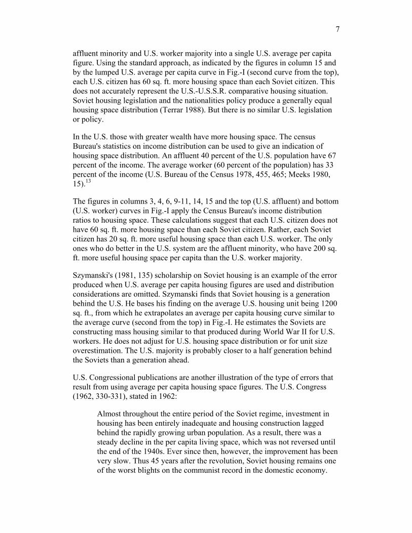
TABLE-I Components for Constructing Fig.-I: Columns 1-41

12 U.S.

housing units in millions

2 Col 1 x 50sq.m

(538 sq. ft.; average U.S. unit size) = total U.S.

space in milns of sq.m.

3 Col 2 x .66 = average U.S.

space occupied by

all affluent in millions of

sq.m.

4 Col 3 x 10.76 sq. ft. (1 m. = 10.76 sq. ft.) = average U.S.

space occupied by all affluent in mil. sq. ft.

1980 88 4400 2904 31247 1970 68 3400 2244 24145 1960 58 2900 1914 20595 1950 41 2050 1353 14558 1940 33 1650 1089 11718 1930 29 1450 957 10297 1920 22 1100 726 7812 1910 20 1000 660 7102

3

TABLE-I (Cont’d) Components for Constructing Fig.-I: Columns 5-8

53 U.S.

population in

millions

6 Col 5 x .40 equals U.S.

affluent population

74 Col 2 divided

by Col 6 = affluent U.S.

per capita space in

sq.m.

84 Col 7 x 10.76 sq. ft. = U.S. affluent per

capita space in sq. ft.

1980 227 90 32 344 1970 203 81 28 301 1960 179 72 27 291 1950 151 60 23 247 1940 132 53 21 226 1930 123 49 20 215 1920 106 42 17 183 1910 52 37 18 194

TABLE-I (Cont’d) Components for Constructing Fig.-I: Columns 9-12

9 Col 2 x .33 =

averspace

occupied by U.S.

majrity in mils sq.m

10 Col 9 x 10.76

sq. ft. = average space occupied by

U.S. majority in millions of

sq. ft.

11 Col 5 x .60 = U.S. majority population in

millions

124 Col 2 divided by Col. 11 = majority per capita U.S.

space in sq. m.

1980 1452 15624 136 11 1970 1122 12073 122 9 1960 957 10297 107 9 1950 677 7285 91 7 1940 545 5864 79 7 1930 479 5154 74 6 1920 363 3906 64 6 1910 330 3443 55 6

4

TABLE-I (Cont’d) Components for Constructing Fig.-I: Columns 13-16

134 Col 12 x 10.76 sq. ft. ft. = U.S. per capita space in

sq.m

14 Col 2 divided

by col. 5 = average U.S.

per capita space in sq. m.

15 Col 14 x

10.76 sq. ft. = average U.S.

per capita space in sq. ft.

165 Soviet per

capita urban housing space

in sq. m.

1980 118 19 204 13 1970 97 17 183 11 1960 97 16 172 9 1950 75 14 151 7 1940 75 13 140 1930 65 12 129 1920 65 10 108 1910 65 11 118 6.3

TABLE-I (Cont’d) Components for Constructing Fig.-I: Column 17

176 Col 16 x 10.76 sq. ft. = Soviet per

capita urban housing in sq. ft.; 1920 & 1940 are estimates based on a loss

of 10 sq. ft. in the Civil War and World War II.

1980 140 1970 118 1960 97 1950 75 1940 (80) 1930 1920 (58) (1922 1910 68 (1913)

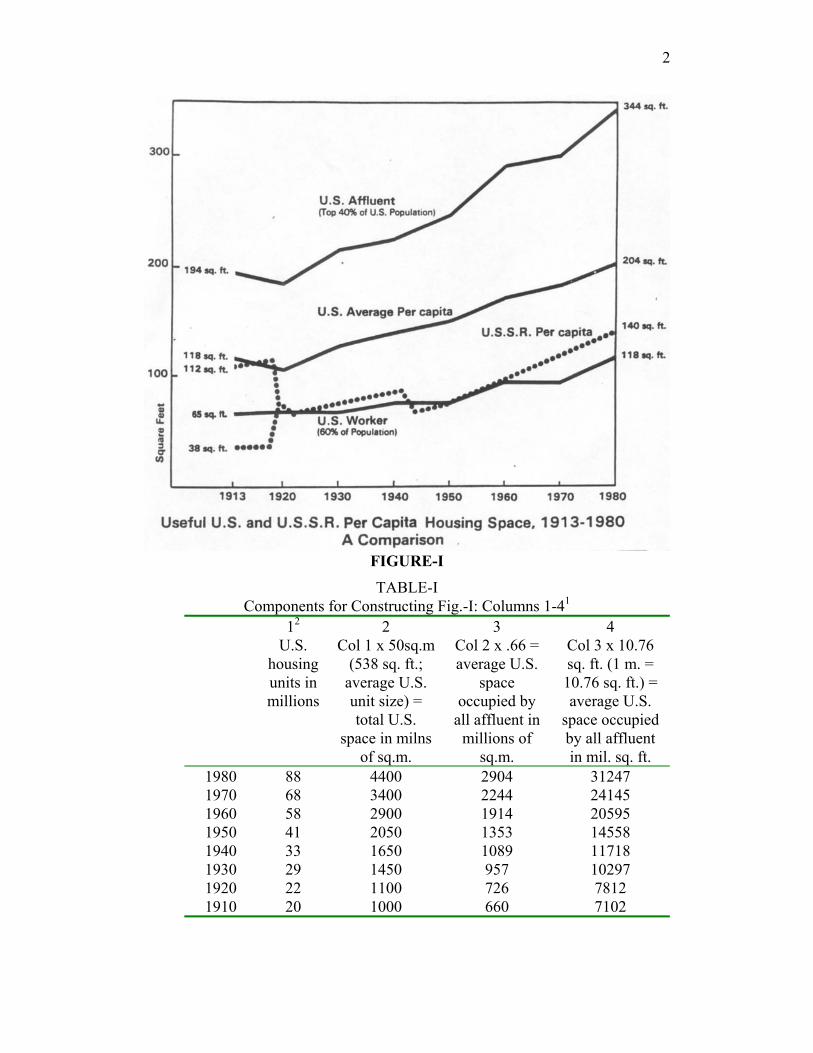
Fig.-I approximates the relationship between Soviet and U.S. housing over most of the twentieth century. Unlike the usual approach, it takes into account housing unit size and the unequal distribution of housing between the affluent minority and the non-affluent majority of the population. In 1913 the U.S. majority had twice as much housing space per capita as the Soviet majority (65 versus 38 square feet). The 1917-1918 revolution in housing raised the Soviet majority to 68 sq. ft. (three square feet above the U.S. majority). The Soviets have maintained the housing lead. The U.S. majority housing space per capita has risen at a rate of one square foot per year, while the Soviet rate has been two square feet per year. The difference is not because the Soviets are building more gross floor space per

5

year. The Soviets average 401 million square feet per year while the U.S. averages 530 million square feet.7 The difference is because the Soviet nationalities policy mandates affirmative action and equal distribution, while the U.S. gives its affluent an average of 355 million square feet and its majority 175 million square feet per year.8

When comparing the Soviets and the U.S., the key statistic is per capita square feet of housing space. It is so important in measuring housing adequacy that it is constitutionally mandated in the Soviet Union (Topornin 1980, 252). U.S. scholars in making comparisons do not generally realize the central importance of this measure. Most of their studies rely on unit or room counts. Because these measures do not account for the size of units and rooms or their distribution, they overstate U.S. majority housing.9 The underdeveloped nature of U.S. housing scholarship is reflected in the failure of the U.S. government to even collect per capita square feet statistics.10

The approximation of per capita square feet as presented in Fig.-I is based on the limited studies of unit and room size that are available and which are discussed in footnote eleven, and on the formula:

Average sq. ft. of useful space per person = (column 13)

total number average useful housing of U.S. housing space per unit units (column 1) X (column 2) total U.S. population (column 5)

The calculations for this formula call for the data and computations in columns 1 to 15 of Table-I, Components for Constructing Fig.-I.

Estimating Unit Space: A 538 Square Foot Average (Column 2)

In calculating housing space square footage per capita, a main step is estimating average square feet per unit. A review of prior unit size studies made over the years gives the parameters for an estimation of 538 square feet of useful housing space.11

There are three different square foot measurements of housing space: gross, useful and livable. U. S. statistics are typically gross housing space measurements. Gross housing space measures from the perimeter of the outside walls and includes all stories or floors. The Soviets do not use gross measurements, only useful and livable ones. The useful measure excludes basements, attics, elevator shafts, exterior hallways, lobbies, thickness of walls, columns and stairs, all of which amount to 25 percent of total area. The livable measure excludes even more and is the square footage on which Soviets pay rent. In addition to that excluded by the useful measure, it excludes kitchens,

6

bathrooms, interior hallways, closets and utility areas.

The Soviets publish their statistics in terms of useful space. U.S. scholars and the U.S. Congress use livable space, the minimal measure, when discussing Soviet housing space (Sosnovy 1954, 6; U.S. Congress 1962, 330). Illustrative of American scholarship in approaching Soviet housing statistics is Morton (1980, 256), who writes:

Soviet housing statistics are invariably reported in square meters of housing space (the total useful space in a unit that includes kitchen, bathroom, corridors and storage area) and not in sq. m. of living space (based on the number of rooms in a unit) which every citizen goes by. To calculate living space from housing space figures, I have used a correction factor of .67 which is used for Moscow, the only city for which aggregate living space data are available.

Using a gross housing space measure, the U.S. Bureau of the Census in its construction starts square footage figures overstates U.S. housing space by counting space that is not useful or livable (U.S. Federal Housing Administration 1960, 13; Building Officials Code Administrators International 1983, 29, 31). The Soviet scholar Fleishits (1976, 36), is accurate in suggesting that in order to be comparable, either Soviet useful or livable space statistics have to be increased upward or U.S. gross space statistics have to be adjusted downward. He writes:

Housing accommodation is calculated in the USSR in terms of the free floor area of living area only and does not include the area of kitchens, hallways, etc. Sixty square meters of living space is equivalent, for example to more than 900 square feet in Great Britain.

To be accurate as a measure of housing adequacy and to be comparable to the Soviet measurements, U.S. Bureau of the Census figures must be reduced by 25 percent to obtain the useful space measure. It must be reduced 58 percent (25 + 33 percent), if comparisons are to be made with Soviet statistics of livable space employed by scholars and the U.S. Congress.12

With adjusted multifamily housing average floor space being in the 400 sq. ft. range, and single family housing in the 500 to 600 sq. ft. range, the 538 sq. ft. average per unit figure used in Fig.-I calculations is a reasonable overall useful space estimation. It is within the median range of sizes discussed in prior studies, if basements, attics, elevator shafts, built in garages, lobbies, hallways, storage and utility areas are eliminated.

Distribution (Columns 3, 4, 6, 10, 11, 14 And 15)

In addition to unit size, the other main consideration in constructing an accurate measure of housing adequacy is distribution. The standard approach is to lump the

7

affluent minority and U.S. worker majority into a single U.S. average per capita figure. Using the standard approach, as indicated by the figures in column 15 and by the lumped U.S. average per capita curve in Fig.-I (second curve from the top), each U.S. citizen has 60 sq. ft. more housing space than each Soviet citizen. This does not accurately represent the U.S.-U.S.S.R. comparative housing situation. Soviet housing legislation and the nationalities policy produce a generally equal housing space distribution (Terrar 1988). But there is no similar U.S. legislation or policy.

In the U.S. those with greater wealth have more housing space. The census Bureau's statistics on income distribution can be used to give an indication of housing space distribution. An affluent 40 percent of the U.S. population have 67 percent of the income. The average worker (60 percent of the population) has 33 percent of the income (U.S. Bureau of the Census 1978, 455, 465; Meeks 1980, 15).13

The figures in columns 3, 4, 6, 9-11, 14, 15 and the top (U.S. affluent) and bottom (U.S. worker) curves in Fig.-I apply the Census Bureau's income distribution ratios to housing space. These calculations suggest that each U.S. citizen does not have 60 sq. ft. more housing space than each Soviet citizen. Rather, each Soviet citizen has 20 sq. ft. more useful housing space than each U.S. worker. The only ones who do better in the U.S. system are the affluent minority, who have 200 sq. ft. more useful housing space per capita than the U.S. worker majority.

Szymanski's (1981, 135) scholarship on Soviet housing is an example of the error produced when U.S. average per capita housing figures are used and distribution considerations are omitted. Szymanski finds that Soviet housing is a generation behind the U.S. He bases his finding on the average U.S. housing unit being 1200 sq. ft., from which he extrapolates an average per capita housing curve similar to the average curve (second from the top) in Fig.-I. He estimates the Soviets are constructing mass housing similar to that produced during World War II for U.S. workers. He does not adjust for U.S. housing space distribution or for unit size overestimation. The U.S. majority is probably closer to a half generation behind the Soviets than a generation ahead.

U.S. Congressional publications are another illustration of the type of errors that result from using average per capita housing space figures. The U.S. Congress (1962, 330-331), stated in 1962:

Almost throughout the entire period of the Soviet regime, investment in housing has been entirely inadequate and housing construction lagged behind the rapidly growing urban population. As a result, there was a steady decline in the per capita living space, which was not reversed until the end of the 1940s. Ever since then, however, the improvement has been very slow. Thus 45 years after the revolution, Soviet housing remains one of the worst blights on the communist record in the domestic economy.

8

A more accurate evaluation is that the Soviets have over the years outperformed the U.S. in housing investment and improvements for the majority. The U.S. Congress employs a double standard. Congress created and funds the U.S. public housing program. In its National Housing Act of 1949 Congress declared that every U.S. citizen should have decent housing. It established a 10 year plan in which .8 million units would be built for the most needy. The Soviets build that amount in 10 months. It took the Congress 23 years to reach its .8 million goal (Starr 1977, 27).14 U.S. cities generally have no laws restricting the number of people who can occupy a housing unit. Where such laws do exist, they require only 50 sq. ft. or less gross space per person. Under such laws, ten people in an average-sized two-bedroom apartment is legal.

Scholars sometimes fail to take into account the distribution of Russian housing space prior to 1918 and the housing space lost in the Civil War and World War II. This results in a negative assessment of Soviet housing performance. Morton (1980, 235-236) is illustrative:

Of all Soviet urban problems, housing remains the most intransigent. The tsarist legacy in housing was dismal. Under Stalin, conditions worsened. Soviet citizens suffer from the poorest housing of any industrialized nation.

The tsarist legacy may have been dismal. But as indicated in Fig.-I, the legacy, once distributed to the Soviet masses, gave them more housing space than the U.S. majority. Further, under Stalin conditions did not worsen, but improved and at a faster rate than for the U.S. majority.

Conclusion

U.S. scholarship underestimates Soviet and overstates U.S. housing space. The per capita unit and room measure used by the U.S. Bureau of the Census does not take into consideration room and unit size, or that the room may be a garage, basement, attic, porch, kitchen, dining room or shack, or that there is unequal distribution of rooms and units between the affluent and the majority.

Perhaps the 538 sq. ft. estimated unit size is short of the mark. Certainly it is a challenge to the 1200-1500 sq. ft. figure used by scholars and which in fact is the gross space of single family new housing starts. New single family housing starts do not take into consideration multiple family dwellings (apartments) and mobile homes, which together account for 50 to 75 percent of new housing. Nor does the new housing starts figure consider the 99 percent of housing stock that is not new, nor the unequal distribution between affluent and majority, nor that as a gross measure, a significant percentage of the figure is neither useful or livable.

Perhaps it is an incorrect assumption to apply to housing space the U.S. Bureau of the Census ratio concerning income: the affluent (40 percent of the population)

9

gets 66 percent of the income and the majority (60 percent) gets 33 percent. Perhaps housing is not as unequally distributed as income. Or perhaps it is even more unequally distributed. Certainly the affluent have more housing space than the majority.

The Bureau of the Census has the capacity to produce a definitive housing space measure. It already measures square footage for new housing starts, and unit and room counts for all housing in the decennial census. The next step is to include a useful per capita square footage question in the 1990 decennial census. The Soviets produce a per capita square footage measure; there is no reason the U.S. cannot do likewise. If indeed the Soviets are outperforming the U.S., the majority might consider shifting the U.S. housing emphasis from the free market to the planned sector, just as it does already for roads, schools, the judiciary, social security, the military, public utilities, banking and mortgage insurance and the post office. The planned housing sector (public housing) may, as the Soviets demonstrate, have a greater ability for serving majority needs than the free market system.

The defense industry gets unlimited government (socialized) funding because it year in and year out plays the Soviet card, the supposed Soviet military superiority. The majority and their labor unions in the building trades, their homeowners, tenants and homeless organizations and the building industry generally could learn a lesson. Their federal programs such as Housing Development Action Grants and Lower-Income Housing Assistance are a defense issue. The strength of the military comes from its defending the system which serves the majority's interest. The soldiers are part of the majority, not of the affluent. Ultimately they and the society which produces them will not defend a system that is not in their interest. The czar and the affluent whom he represented learned this the hard way, when "their" army took sides with the revolution.

References

Alimov, A.A. Soviet Union 50 Years: Statistical Returns. Moscow: Progress Publishers, 1969.

Andrusz, G. D. Housing and Urban Development in the USSR. New York: State University Press, 1984.

Atkinson, A. "On the Measurement of Inequality." Journal of Economic Theory 2 (New York: 1970): 244-263.

Atkinson, W. P. Housing USA. New York: Simon-Boardman, 1954.

Bauman, J. F. Public Housing, Race and Renewal: Urban Planning in Philadelphia,

10

1920-1974. Philadelphia: Temple University Press, 1987.

Building Officials and Code Administrators International, The BOAC Basic National Building Code. Country Club Hills, Ill.: BOAC, 9th ed., 1983.

Carole, C. Analysis of the Floor Area Per Unit in City-Financed Limited Profit Housing Projects. New York: Housing and Redevelopment Board, 1963.

Ceresto, S. "Socialism, Capitalism and Inequality." Insurgent Sociologist 11 (Binghampton, N.Y.: Spring 1982): 5-38.

Cheboksarov, N. N., Zhukov, K. V. "Housing and Population." Great Soviet Encyclopedia 9 (New York: Macmillan, 1973-1985): 248-252.

_______."Housing." Great Soviet Encyclopedia 31 (New York: Macmillan, 1973-1985): 20-25, 286.

Clem, R. S. Research Guide to the Russian and Soviet Censuses. Ithaca, N.Y.: Cornell University Press, 1986.

DiMaio, A. J. Soviet Urban Housing Problems and Policies. New York: Praeger, 1974.

Fleishits, Y. The Civil Codes of the Soviet Republics. Moscow: Progress Publishers, 1976.

Gervas, T. The Myth of Soviet Military Superiority. New York: Harper and Row, 1986.

Gilman, C. P. Women and Economics. New York: Macmillan, 1898.

Jasny, N. The Soviet 1956 Statistical Handbook: A Commentary.East Lancing: Michigan State University Press, 1957.

Josowitz, A. "Housing Statistics: Published and Unpublished." Monthly Labor Review 92 (Washington, D.C., December 1969): 50-55.

Kerblay, B. Modern Soviet Society. New York: Pantheon, 1977.

Khalfina, R. State Property in the USSR. Moscow: Progress Publishers, 1980.

Kirschner, D. S. City and Country: Rural Responses to Urbanization in the 1920s. Westport, Conn.: Greenwood Press, 1970.

Knowles, M. Industrial Housing. New York: Arno Press, 1920.

Kumm, K. Living Standards in the Estonian SSR. Tallinn, Periodika, 1980.

Lampman, R. J. The Share of Top Wealth-Holders in National Wealth. Princeton, N.J.: Princeton University Press, 1962.

11

Lane, H. U. The World Almanac and Book of Facts. New York: Newspaper Enterprise, 1983.

Lenski, G. Power and Privilege: A Theory of Social Stratification. New York: Viking, 1966.

Lorring, W. C. Housing and Social Problems. 3 (1956): 160-168.

Mandel, W. "Impressions," Citizen Diplomat 7 (San Francisco: Fall 1986).

_______. Soviet But Not Russian: The "Other" Peoples of the Soviet Union. Palo Alto, Cal.: University of Alberta Press, 1985.

Meeks, C. B. Housing. Englewood Cliffs, N.J.: Prentice-Hall, 1980.

Michailov, E. C. "The Housing Problem in the Contemporary Stage." S Sh A 25 (Moscow, March 1986): 49-57.

Montgomery, R. Housing in America: Problems and Perspective. New York: Bobbs-Merrill, 1979.

Morris, E. W. Housing: Family and Society. New York: Wiley, 1978.

Morton, H. "Who Gets What, When and How? Housing in the Soviet Union." Soviet Studies 32 (Oxford: April 1980), 235-259.

Quandolo, J. The Constitutionality of Housing Codes: A Survey of the U.S. Supreme Court. Washington, D.C.: National Association of Housing and Redevelopment Officials, 1961.

Riley, H. E. "Evolution in the Worker's Housing Since 1900." Monthly Labor Review 81 (Washington, D.C., 1958): 854-861.

Schutz, R. "On the Measurement of Income Inequality." American Economic Review 41 (Princeton, N.J.: 1951): 107-122.

Smith, B. G. "The Material Lives of Laboring Philadelphians:1750 to 1800." William and Mary Quarterly 38 (Williamsburg, Va., April 1981): 166-176.

Sosnovy, T. The Housing Problem in the Soviet Union. New York: Research Program on the USSR, 1954.

Starr, R. America's Housing Challenge. New York: Hill and Wang, 1977.

Sternlieb, G. S. "Death of the American Dream House." Housing 1971-1972: An AMS Anthology (New York: AMS, 1975): 492-498.

_______. "The Sociology of Statistics: Measuring Substandard Housing." Housing 1973-

12

1974: An AMS Anthology ( New York: AMS: 1976): 335-341.

_______. America's Housing: Prospects and Problems. New Brunswick, N.J.: Rutgers University Press, 1980.

Stiglitz, J. "Distribution of Income and Wealth Among Individuals." Econometrica 37 (Evanston, Ill.: 1969): 382-397.

Straus, N. Two-Thirds of a Nation: A Housing Program. New York: Knopf, 1952.

Swell, J. W. The United States and World Development: Agenda 1977. New York:Praeger, 1977.

Szymanski, A. Human Rights in the Soviet Union. London: Zed Press, 1981.

Terrar, T. "The Right to Housing in the Soviet Union: A Book Review Essay." GeoJournal (Helmstedt, FRG) 17 (June, 1988): 151-154.

Topornin, B. The New Constitution of the USSR. Moscow: Progress Publishers, 1980.

Turner, J. H. American Society: Problem of Structure. New York: Harper and Row, 1976.

United Nations. Compendium of Housing Statistics: 1975-1977. New York: Department of International Economic and Social Affairs, 1980.

U.S. Bureau of the Census. Catalogue of Publications 1946 - 1972. Washington, D.C.: Department of Commerce, 1972.

_______. Historical Statistics of the US: Colonial Times to 1970. Washington, D.C.: Department of Commerce, 1975a.

_______. Construction Reports: New One-Family Homes Sold and for Sale. Washington, D.C.: Department of Commerce, 1975b.

_______. Statistical Abstract of the U.S.: 1978. Washington, D.C.: Department of Commerce, 1978.

_______. User's Guide: Population and Housing, 20th Census, 1980. Washington, D.C.: Department of Commerce, 1980.

_______. Construction Report, Series c25: Characteristics of New Housing, 1984. Washington, D.C.: Department of Commerce, 1985a.

_______. Statistical Abstract of the U.S.: 1985. Washington, D.C.: Department of Commerce, 1985b.

U.S. Bureau of Labor Statistics. "Characteristics of New One-Family Houses: 1954-1956." Monthly Labor Review 76 (Washington, D.C, May 1957), 572-575.

13

U.S. Bureau of Labor Standards. Housing for Migrant Workers: Labor Camp Standards, Bulletin 235. Washington, D.C.:Department of Labor, November 1962.

U.S. Congress. Consumption in the USSR: An International Comparison. Washington, D.C.: Joint Economic Committee, 1981.

_______. Dimensions of Soviet Economic Power. Washington, D.C.: Joint Economic Committee, 1962.

_______. The Federal Response to the Homeless Crisis. Washington, D.C.: Subcommittee of the House Committee on Government Operations, 1985.

U.S. Federal Housing Administration. Minimum Property Requirements for Properties of Three or More Living Units, 1202-c. Washington, D.C.: Government Printing Office, 1960.

_______. Minimum Property Standards for One and Two Living Units (No-300, 602-3.1). Washington, D.C.: Government Printing Office, 1960.

_______. How FHA Measures a House (No-948). Washington, D.C.: Department of Housing and Urban Development, 1966a.

_______. Minimum Property Standards for Low Income Housing (PG-1, part vi, L602-3.1). Washington, D.C.: Department of Housing and Urban Development, 1966b.

U.S. Housing Authority. Summary of Standards and Requirements for USHA-Aided Projects. Washington, D.C.: Federal Works Agency, February 1940.

USSR Central Statistical Board, The USSR in Figures for 1978: Statistical Handbook. Moscow: Statistike, 1979.

Wheaton, W. "Housing." Collier's Encyclopedia 12 (New York: Macmillan, 1978): 318.

Whittenburg, J. "Measuring Inequality: A Fortran Program for the GENI Index, Schutz Coefficient and Lorenz Curve." Historical Methods 10 (Washington, D.C.: 1977): 77-84.

Endnotes

1All housing statistics are in terms of useful space.

2Housing unit statistics (column 1) are from U.S. Bureau of the Census 1975a, part 1, 646; U.S. Bureau of the Census 1984, 731; Morris 1978, 110; Meeks 1980, 21. National housing statistics were collected for the first time in a decennial census in 1940. The inclusion of housing questions, which has

14

continued in each decennial census since then, reflected the housing rights expectations mobilized during the depression (Bauman 1987). The housing section of the 1940 and subsequent censuses focused on the need of repair. It and more recent censuses did not enumerate amount of floor space per unit or per room. After the 1940 census was completed, the census bureau made a rough estimate of the number of units existing from 1890 to 1930 by equating the "number of households" category used in the earlier decennial censuses with housing units. The definition and criteria for the "household" category approximated the unit definition (Sternlieb 1976, 236; U.S. Bureau of the Census 1975a, part 2, 634; U.S. Bureau of the Census 1980, 15).

The Census Bureau also collected construction start figures for various categories of new housing units as part of its Census of Business for 1929, 1935 and 1938. It published similar figures for 1967 as part of its Economic Census (U.S. Bureau of the Census 1972, 45). Currently it publishes annual construction start figures in its series, Characteristics of New Housing (U.S. Bureau of the Census 1985a).

3Population statistics (column 5) are published in U.S. Bureau of the Census 1975a, 8; Lane 1983, 197.

4Average per capita majority and affluent housing space in sq. ft. (columns 7, 8, 12 and 13) is obtained by the formula:

average sq. ft. of housing per affluent U.S. citizen =

total U.S. housing space (Col 2) x .66 . 40 x U.S. population (Col 5)

Column 3 Column 6 =

Column 8

average sq. ft. of housing per U.S. majority =

total U.S. housing space (Col 2) x .33 .60 x U.S. population (Col 5)

Column 9 Column 11 =

Column 12

5Alimov (1969, 252) lists (column 16) the 1913 and 1950 figures. He also has 10 sq. m. per capita for 1966. DiMaio (1974, 34) lists the 1960 (8.8 sq. m.) and 1970 figures; Cheboksarov (1973-1985, vol. 31, 25), lists the 1980 figure. Jasny (1957) and Clem (1986) give a history of Soviet statistics. The Soviets lost one sq. m. (10.76 sq. ft) housing space per capita in their civil war and another one sq. m. in World War II. Cheboksarov (1973-1985, vol. 9, 253) quotes the Civil War housing space loss as 14 percent.

The per capita housing loss for the Civil War was obtained by the formula:

15

per capita housing loss =

Russian 1913 per capita percentage of housing urban housing space X lost (1913-1921)

= 6.3 x .14 = 1 sq. m. per capita

Cheboksarov (1973-1985, 250, 252) quotes the World War II housing space loss as 70 million sq. m., making 25 million people homeless. The per capita housing loss for World War II is given by the formula:

per capita = housing loss

Soviet 1940 per percentage of capita urban X population that lost housing space their housing space

And

percentage of population that lost their housing space =

population losing housing total housing population in 1940

25 million = 194 million = 13 percent

6In 1913 the total Russian housing space (column 17) was unevenly distributed. This is illustrated by the dotted curve in Fig.-I for the year 1913. The Fig.-I estimate was made by using the same procedure as was applied to the U.S. data discussed in the text. This indicates Russian workers/peasants had 38 sq. ft. per capita in 1913 and the Russian affluent 112 sq. ft. per capita of housing space. The formula for obtaining these figures has three parts. The first part of the formula for the 1913 figure is:

amount of housing space in millions of sq. m. = owned by affluent

total urban + rural Russian 1913 housing X .66 = space in mil. sq. m.

1000 mil. sq. m. X .66 = 666 mil. sq. m.

A total Russian housing space statistic was not published, only an urban statistic. Alimov (1969, 252) lists the total urban housing space in millions of sq. m. for 1913 as 180. For comparative purposes Alimov also lists useful floor space in millions of sq. m. for 1926 as 216, for 1940 as 421, for 1950 as 513, and for 1960 as 958. Cheboksarov (1973-1985, vol. 9, 250) and DiMaio (1974, 34) list 1970 as 1529; Cheboksarov (1973-1985, vol. 31, 286) lists 1980 as 2200.

The total urban plus rural 1913 figure was approximated, using the formula:

16

total urban + rural 1913 housing in = millions of sq. m.

urban housing space in sq. m. = percentage of total urban to total space

180 mil. sq. m. .18 =

1000 mil. sq. m.

The percentage of urban population is known. It is assumed housing occurs in about the same proportions for rural as for urban population. Cheboksarov (1973-1985, vol. 31, 286) notes that in 1981, one-third of new housing was rural. This was proportional to the rural population. Any disproportion is probably in the direction of more abundant rural housing, since there has been a long term rural migration to the cities. Morton (1980, 249) writes that: "The large scale migration from the countryside to the city has left many abandoned but fully habitable houses in rural areas." Kumm (1980, 61) comments that in Estonia, "Living conditions are better in the countryside where 17 sq. m. of useful housing space are available to each inhabitant." Mandel (1985), Terrar (1988) and Andrusz (1984, 270) discuss Soviet government policy, which since 1918 has been for uniform and proportional development, and the elimination of differences between town and country.

Cheboksarov (1973-1985, vol. 9, 250) lists the percentage of urban Russian population as 18 percent in 1913. For purposes of comparison Cheboksarov lists urban population percentages as 33 for 1940 and 48 for 1959. The same author (1973-1985, vol. 31, 20) lists 63 percent for 1981.

The second part of the formula for the 1913 figure is:

affluent per capita housing space sq. m. =

amount of housing space owned by affluent in sq. m. = affluent population

666 mil. sq. m. 64 mil. people = 10.4 sq m. = 112 sq. ft.

affluent population =

Russian 1913 pop. (i.e., 159 mil.) X .40 =

64 million people

Cheboksarov (1973-1985, vol. 31, 20) lists the Soviet population statistics. For purposes of comparison that Cheboksarov lists 147 millions of people in 1926, 194 in 1940, 179 in 1950, 214 in 1960, 242 in 1970 and 267 in 1981.

The third part of the formula for the 1913 figure is:

17

amount of housing space in millions of sq. m. occupied = by Russian workers/peasants in 1913

total Russian 1913 space = X. .33 =

1000 mil. sq. m X .33 = 333 mil. sq. m.

worker/peasant per capita housing = in 1913 sq. m.

amount of housing space in millions of sq. m. occupied by workers/peasants = worker/peasant population

333 mil. sq. m. 95 mil. people = 3.5 sq. m. 38 sq. ft.

worker/peasant population = Russian 1913

population X .60 = 95 mil. people

For purposes of comparison, the number of Soviet housing units in millions was 4.5 in 1913, 5.4 in 1926, 10.5 in 1940, 12.8 in 1950, 24 in 1960, 38 in 1970 and 55 in 1980. United Nations (1980, 158) lists 31 million urban units in 1965, with an average 1.3 persons per room. Generally, Soviet unit statistics are not published, but can be calculated as in the 1913-1980 figures above, with the formula:

total housing units in millions =

total Soviet housing space in millions sq. m. average unit size space

The average unit size in sq. m. for 1913 through 1960 was 40, for 1970 was 45 and for 1980 was 51. These figures are based on Cheboksarov (1973-1985, vol. 9, 248). He writes that by 1925 a program of standard design multistory housing was in place. Apartments were predominantly two separate rooms with a total area of 40-45 sq. m. Most apartments were intended for one family but several families usually lived in them. Kerblay (1979, 55, 70) remarks that the several families were generally related: a widowed mother or father would live in and help raise the grandchildren for working parents. The same "communal" housing occurred and occurs in the U.S. Unlike singles and childless couples, couples with children get priority for newly built housing. If couples with children live in a parent's home or have a parent live with them, it is not generally from necessity. U.S. feminists as early as Charlotte Gilman in the 19th century advocated such "communal" living along with day care and shared cooking, dining and laundering facilities as a liberating achievement. According to Mandel (1986, 7), the Young Communist League in the Soviet Union and many citizens believe in

18

semi-communal complexes for young marrieds with children. In 1986 3000 delegates of the Youth Housing Complex movement held a conference in Moscow.

The 1970 and 1980 figures for unit size are calculated from total square meters of floor space and unit quantities given by Cheboksarov (1973-1985, vol. 31, 287) and Alimov (1969, 250). Thus the fifth (1951-1955) five year plan in sq. m. was 38, the sixth (1956-1960) was 39, the seventh (1960-1965) was 42, the eighth (1966-1970) was 45, the ninth (1971-1975) was 48 and the tenth (1976-1980) was 51. Kumm (1980, 61) notes that in Estonia, the average unit, which was a three room apartment, was 43 sq. m. in 1950 and 65 sq. m. in 1980.

7The square foot yearly average was obtained by the formula: total sq. m. (1980) - total sq. m. (1913) 1980-1913 X 10.76 sq. ft.

i.e., U.S. Sq. ft. yearly average =

4400 mil. sq. m. – 1100 mil. sq. m. 67 years

= 530 mil. sq. ft.

Soviet sq. ft yearly average =

3500 mil. sq. m. – 1000 mil. sq. m. 67 years = 401 mil. sq. ft.

For U.S. total sq. m. see Table-I, Components for Constructing Fig.-I, column 2. The Soviet total sq. m. figures above were obtained by the formula:

Soviet total sq. m. space in 1913/1980 =

total urban (1913/1980) percentage of total urban to whole country

i.e.,

180 mil. sq. m. 18% = 1000 mil. sq. m. in 1913

2200 mil. sq. m. 63% = 3500 mil. sq. m. in 1980

For Soviet urban total sq. m. and urban percentage figures used above, see Table-I, Components for Constructing Fig.-I, column 17.

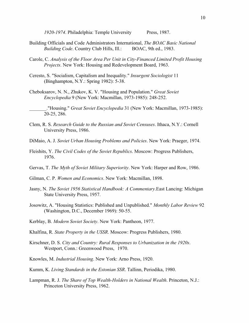
8The affluent and majority yearly housing square foot average was obtained by the formula:

affluent/majority percentage of annual floor space X total annual floor space

19

i.e.,

67% x 530 mil. sq. ft. = 355 mil. sq. ft. average affluent housing space

33% x 530 mil. sq. ft. = 175 mil. sq. ft. average majority housing space

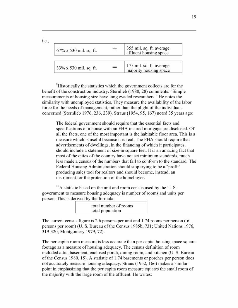
9Historically the statistics which the government collects are for the benefit of the construction industry. Sternlieb (1980, 28) comments: "Simple measurements of housing size have long evaded researchers." He notes the similarity with unemployed statistics. They measure the availability of the labor force for the needs of management, rather than the plight of the individuals concerned (Sternlieb 1976, 236, 239). Straus (1954, 95, 167) noted 35 years ago:

The federal government should require that the essential facts and specifications of a house with an FHA insured mortgage are disclosed. Of all the facts, one of the most important is the habitable floor area. This is a measure which is useful because it is real. The FHA should require that advertisements of dwellings, in the financing of which it participates, should include a statement of size in square feet. It is an amazing fact that most of the cities of the country have not set minimum standards, much less made a census of the numbers that fail to conform to the standard. The Federal Housing Administration should stop trying to be a "profit" producing sales tool for realtors and should become, instead, an instrument for the protection of the homebuyer.

10A statistic based on the unit and room census used by the U. S. government to measure housing adequacy is number of rooms and units per person. This is derived by the formula:

total number of rooms total population

The current census figure is 2.6 persons per unit and 1.74 rooms per person (.6 persons per room) (U. S. Bureau of the Census 1985b, 731; United Nations 1976, 319-320; Montgomery 1979, 72).

The per capita room measure is less accurate than per capita housing space square footage as a measure of housing adequacy. The census definition of room included attic, basement, enclosed porch, dining room, and kitchen (U. S. Bureau of the Census 1980, 15). A statistic of 1.74 basements or porches per person does not accurately measure housing adequacy. Straus (1952, 166) makes a similar point in emphasizing that the per capita room measure equates the small room of the majority with the large room of the affluent. He writes:

20

Definitions of terms are essential. A "6-room house" or a "4 1/2-room apartment" may mean a dwelling of 400 square feet or 1000 square feet. A housing project described as having "an acre of parks for use of tenants" or having "buildings which cover only 25 percent of the site" may be desirable and uncrowded or may be instead, a new superslum with fancy gadgets, colored tile baths - and 500 people packed into every acre. The only dependable measures of congestion are (a) size of the dwelling and (b) the number of persons living on an acre of ground.

11A researcher in the 1920s (Knowles 1920, 297-298), for example, found the typical skilled, high paid worker's house to be 576 gross sq. ft., based on a study of 18 house styles. This included a living room (168 square feet), dining room (120 square feet), two bedrooms (120 and 80 sq. ft.) and bathroom (35 sq. ft.). Lower paid workers lived with private families or in boarding houses or in dorms with double bunkbeds or with two or more to a bed (Knowles 1920, 334).

Similar gross sq. ft. dimensions were typical of the 1940s (between 420-550 sq. ft. for two bedrooms and 440-570 sq. ft. for three bedrooms) and 1950s (552 sq. ft. with two bedrooms, a living room, kitchen and bath) (U. S. Housing Authority 1940, 25-26; Atkinson 1954, 135). The Federal Housing Administration set 220 sq. ft. as a minimum requirement for an efficiency apartment in the housing which it helped insure (U. S. Housing Administration 1948, 24). Half of all the apartments built with FHA assistance in the 1950s were 3 1/2 rooms or less (350 sq. ft.) (Straus 1952, 126).

During the 1950s government and non-government organizations set ideal gross sq. ft. per capita and unit size norms. The Los Angeles Housing Authority had a 575 sq. ft. unit minimum. But 480 sq. ft. units were commonly built by the large scale builders able to do without government financing (Straus 1952, 86).

While 1088 gross sq. ft. was an ideal for a 1950s six room house, in actuality six room houses averaged 674 sq. ft. (Straus 1952, 28). A 672 sq. ft. pattern (24 x 28 ft.) was widely used by conventional builders and prefabricators in the 1950s (Straus 1952, 54). The American Public Health Association set 450 sq. ft. as the norm for a single person, 750 sq. ft. for a couple, and 1000 sq. ft. for a family of three. But as C. E. Winslow (Straus 1952, 86), chair of the Public Health Association said at the time:

Very little of the housing erected meets these standards. In most of our mushrooming suburban housing developments today you cannot tell the house from the garage. If we progress much further in this direction, you won't be able to tell the house from the letter box.

Minimum average floor space in the 1960s and 1970s according to one source was 140 gross sq. ft. per person (Wheaton 1978, 318). The Federal Housing

21

Administration in 1960 set 420 sq. ft. as the minimum property standard for a one bedroom unit (U. S. Federal Housing Administration 1960, 32). In 1966 the Federal Housing Administration listed as minimum property standards 380 sq. ft. (one bedroom unit), 450 sq. ft. (two bedroom unit) and 550 sq. ft. (three bedroom unit) (U. S. Federal Housing Administration 1966). Wheaton (1978, 318) states that during this period the average dwelling contained 1200 gross sq. ft. One-third to one-half of this (400-600 sq. ft.) was basements, attics, halls, closets and utility rooms. In New York City during the 1960s, 523 sq. ft. was the median for a one bedroom unit, 679 sq. ft. for a two bedroom unit and 838 sq. ft. for a three bedroom unit (Carole 1963, 1-2). In his research Carole found the New York median to be too high, because of finance and construction costs. He suggested it be lowered to 430 sq. ft. (one bedroom), 590 sq. ft. (two bedrooms) and 750 sq. ft. (three bedrooms).

Starting in 1954 the Bureau of Labor Statistics and after 1959 the Census Bureau when it took over the job, began to make field surveys in selected areas and to include in its statistics on construction starts, the square foot space for new non-farm single family private housing. The median space for the single family starts in 1958 was 1200 sq. ft. and has ranged up to 1500 sq. ft. over the years. This figure is a gross housing space measurement. It includes both finished and unfinished basements and attics at least five feet in height, closets, halls, utility and laundry rooms, built in garages, bathrooms and kitchens (U. S. Bureau of Labor Statistics 1957, 572-575; U. S. Bureau of the Census 1972, 46; U. S. Bureau of the Census 1975b; U. S. Bureau of the Census 1985a, 31, 34; U. S. Federal Housing Administration 1966, 5; Josowitz 1969, 50-55; Riley 1958, 861).

In the 1970s the Census Bureau added to its construction starts, surveys on square footage of multiple family (apartment) units. The median figure (900 sq. ft. per unit) included hallways, lobbies, elevator shafts, basements and attics. U. S. Bureau of the Census 1985a, 41).

12Aside from the misleading nature of using a gross space statistic as a measure of housing adequacy, there are other factors which support a downward adjustment of, for example, the construction start figures of 1200-1500 sq. ft. for a single family unit and 900 sq. ft. for a multiple family unit. Since 1970 mobile homes have accounted for one-third to one-half of new single family housing units. Mobile homes generally have less space than apartments. They are not counted as single family homes. This results in an overestimation of the median measure of single family housing (U. S. Bureau of the Census 1975a, 640; Sternlieb 1975, 492, 496).

Another factor in considering housing size is the housing of those who live in work camps, prisons and similar situations. In the 21 states which set legal standards, 35 to 50 sq. ft. per person of housing space is mandated for farm workers and their families. In trailers 20 sq. ft. of clear space per person is normative (U. S. Bureau of Labor Statistics 1962, 12-13). By government

22

definition, poverty means housing inadequacy. According to government statistics thirty-five million (15 percent of the population) are in poverty. They live in rural and inner city areas. One-third of the U. S. housing stock is rural and another is inner city (Sternlieb 1976, 237; Sternlieb 1980, 9). The housing census includes in its definition of housing unit, items such as shacks, cellars and dormitories. To include such in a measure of housing adequacy is to overstate what is adequate. Speculators use political influence to prevent efforts to increase building code minimum habitable unit floor areas. For example an increase from 400 to 800 sq. ft. was resisted in New York with the argument that "the determination of the size of homes is an improper use of police powers of the state, and has no relation to the safety, health, morals or welfare of the citizen" (Straus 1952, 87; Quandolo 1961).

13Lane (1983, 205) states that the highest 20 percent of the U.S. population has 42 percent of the income and the highest 40 percent has 66 percent of income. Wealth, as a category, is even less evenly distributed than income. Among those who discuss why wealth distribution rather than income distribution is a more accurate measure of equality are Ceresto (1982, 13) and Turner (1976). Housing is part of wealth, not income. Housing is thus probably less well distributed than indicated in Fig.-I (Lampman 1962, 1-2, 8, 136; Lenski 1966; Atkinson 1970; Schutz 1951; Stiglitz 1969; Whittenburg 1977).

14According to Starr, this was because landlord and banking interests tend to have a disproportional influence in the legislature. Public housing decreases profit. The poorest developing nations regularly outperform the U.S. Congress. In the U.S., affluent housing is segregated by law (zoning codes) from majority housing. U.S. housing scholars are affluent and sometimes live their lives in ignorance of majority housing conditions. Overcrowded housing is profitable to landlords who can charge higher prices. It results in the spreading of diseases such as tuberculosis (Lorring 1956, 160-168). The affluent point to the opportunity which the U.S. offers to rise out of poor housing. However, they do not advocate that their own children live in such conditions. The majority U.S. population have similar wishes for their children. They prefer to end poverty, so their children will not have to rise out of it, but rather enjoy the advantages of decent housing. And they prefer not to rise on the backs of the most vulnerable.