NASA / TM--2000-209400

Solving ODE Initial Value Problems With

Implicit Taylor Series Methods

James R. Scott

Glenn Research Center, Cleveland, Ohio

March 2000

https://ntrs.nasa.gov/search.jsp?R=20000034027 2020-04-19T10:15:31+00:00Z

The NASA STI Program Office... in Profile

Since its founding, NASA has been dedicated to

the advancement of aeronautics and spacescience. The NASA Scientific and Technical

Information (STI) Program Office plays a key part

in helping NASA maintain this important role.

The NASA STI Program Office is operated by

Langley Research Center, the Lead Center forNASA's scientific and technical information. The

NASA STI Program Office provides access to the

NASA STI Database, the largest collection ofaeronautical and space science STI in the world.

The Program Office is also NASA's institutional

mechanism for disseminating the results of itsresearch and development activities. These results

are published by NASA in the NASA STI ReportSeries, which includes the following report types:

TECHNICAL PUBLICATION. Reports of

completed research or a major significant

phase of research that present the results ofNASA programs and include extensive data

or theoretical analysis. Includes compilationsof significant scientific and technical data and

information deemed to be of continuingreference value. NASA's counterpart of peer-

reviewed formal professional papers but

has less stringent limitations on manuscriptlength and extent of graphic presentations.

TECHNICAL MEMORANDUM. Scientific

and technical findings that are preliminary or

of specialized interest, e.g., quick releasereports, working papers, and bibliographiesthat contain minimal annotation. Does not

contain extensive analysis.

CONTRACTOR REPORT. Scientific and

technical findings by NASA-sponsored

contractors and grantees.

CONFERENCE PUBLICATION. Collected

papers from scientific and technicalconferences, symposia, seminars, or other

meetings sponsored or cosponsored byNASA.

SPECIAL PUBLICATION. Scientific,technical, or historical information from

NASA programs, projects, and missions,

often concerned with subjects havingsubstantial public interest.

TECHNICAL TRANSLATION. English-

language translations of foreign scientificand technical material pertinent to NASA'smission.

Specialized services that complement the STIProgram Office's diverse offerings includecreating custom thesauri, building customized

data bases, organizing and publishing research

results.., even providing videos.

For more information about the NASA STI

Program Office, see the following:

• Access the NASA STI Program Home Pageat http-//www.sti.nasa.gov

• E-mail your question via the Internet to

help@sti.nasa.gov

• Fax your question to the NASA Access

Help Desk at (301) 621-0134

• Telephone the NASA Access Help Desk at(301) 621-0390

Write to:

NASA Access Help DeskNASA Center for AeroSpace Information7121 Standard Drive

Hanover, MD 21076

NASA / TMm2000-209400

Solving ODE Initial Value Problems With

Implicit Taylor Series Methods

James R. Scott

Glenn Research Center, Cleveland, Ohio

National Aeronautics and

Space Administration

Glenn Research Center

March 2000

Acknowledgments

The author would like to acknowledge valuable technical discussions with Ayo Oyediran, Loren Dill,

Ananda Himansu, Ken Loh, and Shang-Tao Yu.

NASA Center for Aerospace Information712i standard Drive

Hanover, MD 21076Price Code: A06

Available from

National Technical Information Service

5285 PortRoyal Road

Springfield, VA 22100Price Code: A06

Solving ODE Initial Value Problems with

Implicit Taylor Series Methods

James R. Scott

National Aeronautics and Space Administration

Glenn Research Center

Cleveland, Ohio

Introduction

By expanding the solution to the initial value problem

y' = f(t,y) y(to) = Yo (1.1a,b)

in a Taylor series about to, one obtains a local solution which is valid within its radius of

convergence R0. If the series is evaluated at t,, where t, < Ro, one obtains an approx-

imation to y(t,), and the solution may then be expanded in a new series about tl. The

solution may of course then be extended to the point t_, and so forth, so that by a process

of "analytic continuation" one obtains a piecewise polynomial solution to (1.1).

When the derivatives of y can be obtained cheaply, the method of Taylor series, or

analytic continuation, offers several advantages over other methods. Foremost among these

is that a Taylor series solution provides information that is not provided by other methods.

This includes derivative information, local radius of convergence, and the location of poles

in the complex plane. Another advantage is that both the stepsize and order can be easily

changed, so that an optimal stepsize can always be chosen. Finally, Taylor series integration

provides a piecewise continuous solution to the ODE, so that it is never necessary to

interpolate at intermediate points.

Since analytic continuation is efficient only when high order derivatives can be ob-

tained inexpensively, much effort has been made to develop recursive techniques that can

generate the derivatives numerically. The first known attempt to incorporate recursion

into the Taylor series method was by J.R. Airey in 1932 [1]. Miller was the first to employ

a full recurrence scheme in which all series coefficients were calculated numerically, and

the first to develop a systematic approach which was applicable to a class of differential

equations [2,3]. Other early work include s that of Gibbons [4] and Moore [5], who devel-

oped programs that automatically generate the series coefficients for differential systems

in canonical form. Other work concerning automated differentiation is that of Leavitt [6],

Nikolaev [7], Barton et. al. [8,9], Norman [10], Kedem [11], Rall [12], Chang [13], Corliss

and Chang [14], Irvine and Savageau [15], and Savageau and Volt [16].

Of the above, the most complete and systematic treatments of the Taylor series method

are those of Barton, Willers, and Zahar [8,9], Chang [13,17,18] and Corliss and Chang [14],

NASAfYM--2000-209400 1

and Irvine and Savageau[15]. Barton ct.al, were the first to develop and implement a

general purpose algorithm that automatically reduces a given differential system to canon-

ical form and generates the series coefficients without any previous manipulations by the

user. Chang and Corliss developed a similar approach along with computer programs that

are fully portable. Their programs also provide information oll the location and order of

primary singularities. Irvine and Savageau developed highly emcient series methods for

differential equations that can be expressed in the form of an "S-system". Their approach

obviates the need to generate problem-dependent source code for each new problem.

Corliss and Chang and Irvine and Savageau compared their codes with several stan-

dard ODE solvers on the problem set of Hull et.al. [19]. Compared to the IMSL routines

D\TERK (Runge-Kutta method) and DGEAR (variable order Adams method), Corliss

and Chang report that their code was significantly faster for error tolerances in the range

10 -9 to 10 -12 . They conclude that the Taylor series method is superior to tile variable

order Adams method and the Runge-Kutta method when stringent accuracies are required

and when solving small systems. Irvine and Savageau compared their method with two

standard Runge-Kutta schemes, a variable order Adams method, and Gear's method. On

an S-system from cellular biology, they report solution times that were significantly faster

than all four methods for error tolerances ranging from 10 -5 to 10 -55 . In some cases,

their code was faster by one or two orders of magnitude. On Hull's problem set, their

results compared favorably both in terms of solution times and number of flmction eval-

uations. For small error tolerances, their code was up to 20 times faster. One concludes

that the Taylor series method is indeed competitive with other methods, especially when

high accuracies are required.

In this paper we propose an extension of the Taylor series method which improves its

accuracy and stability while also increasing its range of applicability. The basic idea is

to formulate the method as a generalized implicit method. Specifically, given an interval

[t., tn+5], we consider a series solution to (1.1) which is expanded about the intermediate

point t_ + It h, where h is the stepsize and tt is an arbitrary parameter called an expansion

coefficient.

The main results of the paper are the following. (i) We derive the discretization error

for a series solution to (1.1) which is expanded about the point t_ + # h. It is shown that

a series of degree k has exactly k expansion coefficients which raise its order of accuracy.

The increase is one order if k is odd, and two orders if k is even. For k odd, it will be seen

that a class of Turan type, one-stage implicit Runge-Kutta methods are recovered [20]. (ii)

We consider stability for the problem y_ = A y, Re (A) < 0, and identify several A-stable

schemes. (iii) We show that, for all series of degree three or higher, local extrapolation

can be used to increase accuracy by two additional orders. (iv) We discuss variable step

schemes. (v) We present numerical results for a range of problems, including ODE's with

a singular point and stiff systems. Our results indicate that implicit Taylor series methods

are an effective integration tool for most problems.

NASA/TM--2000-209400 2

Taylor Series of Degree One

We assume that f(t, y) is a real-valued function which is analytic at the point (t,_, yn),

and that the problem

y' = f(t,y), y(t,_) = Yn, (2.1a,b)

has a unique, continuous solution which can be expressed as a power series that converges

for all t in the interval It - t,_] < R,_. We denote the stepsize t,_+l - t,_ by h, where

h < Rn.

A Taylor series of first degree expanded about tn gives the equation

h 2

y(tn+l) ---- y(tn) -]- h f(tn, Yn) + -_ f'(_n,Y(_n)), tn < _n < tn+l, (2.2)

from which one obtains Euler's method

y,_+l = yn + h f(t,_,y,,) (2.3)

h 2 IIand its associated discretization error T ff(_n, y(_n)) := y (_,_). The error may also be

expressed by the expansion

h2 h3 h4 f"' (2.4)en+l := y(tn+l) -- Yn+l : _ fin + _ f_n' + -_n + "'"

where f_ := f'(tn, yn), and similarly for ]_' and f'_'.

If the series is expanded about tn+a, one obtains the backward Euler method

Y_+I = Yn + h f(tn+l,y,_+l), (2.5)

where yn+l must be obtained implicitly. By expanding f(tn+l, Y,_+I) in a Taylor series

about (tn, Yn), one derives from (2.5) the discretization error

[h__ h 3 Ofnen+l :---- y(tn+l) -- Yn+l -_ -- ftn + -6-- (2f_ _ + 3-_y f_)

h 4 Ofn Of_ ]+ N (3f" + s f" + 12 f:) + (2.6)

Both the forward and backward Euler methods provide a linear approximation to y

on In := [tn, t_+l]. This approximation can be written

Y,_ = Y,+u + (t - t,+u ) f(t,_+u, Y,_+u), t_ < t < tn+l, (2.7)

where p is zero or one, respectively.

NASA/TM--2000-209400 3

If we define tn+, := tn + #h, where 0 _< # _< 1, Eq. (2.7) becomes a generalized

approximation to y on In. In this case the approximation will pass through the intermediate

value yn+_, which is unknown. By observing that y,_ must equal y,_ when t = tn, one can

see that Y,_+t* must be determined from

_J_+. = yn + l*h f(t,_+., y_+.). (2.Sa)

Note that this is just the backward Euler method for the partial step from t,_ to t_+,.

Once yn+, is determined from (2.8a), one sets t = t_+_, yn = yn+; in (2.7) to obtain

y,_+_ = yn.. + (1 - _) h f(t,,+., y,,+.). (2.8b)

One observes that this is just tile forward Euler method for the partial step from t_,+r, to

tn+1. Thus, two steps are required to advance the solution to t,_+l - a backward Euler

intermediate step followed by a forward Euler final step.

To determine an optimal expansion point tn+u, one obtains the truncation error for

(2.8). Since (2.8a) is the backward Euler method with stepsize p h, one uses (2.6) to obtain

an expansion for y,,+,, which may then be substituted into (2.8b). One gets from (2.6),

yn+, = y,_ + ph fn + (#h)2f_, + T (f_(ph)3" +--_-y fn)i)f",

+ (p.h) 4 (f,,, + 2of_ of:_W f:' + a-g-y-yL) +

Upon expanding f(t,_+., yn+.) about (t.,, y._), and evaluating powers of (Y,_+t_

way of (2.9), one obtains from (2.85)

Yn+I = Yn + h f,_ + #h2 f'_ + #2 ha Of,_ ,(f:"+ w

+ _3 h4 (r"' 0% 0]" ,V"" + 2W:" + awf )

The error expansion for (2.8) isthen

enq-I

+ O(h_). (2.10)

h Of,, ]:= y(tn.t) - Yn+, = (1-2.)-_-f/_ + -_ (1-3p2) f_ ' - 3#2--_-y f_

h 4

. _-_ [(1 - 4,')f"'on - p3 (8 --_-yfnOf'_,, . 12_0__y0f_f:)] * O(h5). (2.11)

NASA/TM--2000-209400 4

1 the marching schemebecomesTaking # = _,h

Yn+½ = Yn + -_ f(tn+½,Y..+½)(2.12a)

Yn+l =

with discretization error

h

Yn+½ + -_ f(t,_+½,y,_+½), (2.12b)

h3 of. f.)e.+, --- 25 (f" - 3

h4 (fro _ 20fn Of'n+ _-_ _Jn -_y fin' - 3--0-_y f,',) + O(h5) ' (2.13)

1 thus leads to a second-order scheme. Ill view of the central expansionThe choice p =

point tn+ ½, we will refer to (2.12) as the "centered Euler nlethod".

It should be noted that, corresponding to (2.12), the linear expansion (2.7) approx-h 2

imates y(t) with an error at most equal to W lf_[ + O(h3)" This is one-fourth the error

bound on (2.7) corresponding to the forward and backward Euler methods.

We should also mention that the explicit halfstep (2.12b) can be equivalently expressed

as

Yn+l = Y,_ + h f(tn+½,Y.+]). (2.14)

When written in this form, it is clear that the centered Euler method is similar to the

trapezoidal ruleh

Yn+l = Yn + -_ [f(tn, y,_) + f(t,_+l, yn+l)]. (2.15)

It is also similar to the one-stage Gauss implicit scheme [21], [22],

Yn+l = Yn + kl (2.16a)

kl = h f(tn+½,Yn + ½kl),

which is equivalent to the implicit midpoint rule [22],

(2.16b)

yn+l = yn + hf(tn+½, ½(y,_ + Y_+I))- (2.17)

It can be shown in fact that the centered Euler method and the implicit midpoint rule are

equivalent schemes. One can also show that the trapezoidal linear approximation to y on

yT(t) = Yn + (t--tn) f(tn, y_)+ f(t_+l,y_+l) (2.18)2

h 2approximates y with a maximum error equal to that of the centered Euler method, _- ]f,',I +

O(h3). One concludes that these three schemes offer nearly identical benefits over the

forward and backward Euler methods.

NASA/TM--2000-209400 5

Taylor Series of Degree Two

Analogous to Eq. (2.7), a Taylor series of second degree expanded about the point

t,,+_ approximates y on I,, by

(t-tn+.)Y_, = Y,_+u + (t-t,.+u)f(t,,+,,y,,.+,) + 2 f'(t,,+t,,y,+u ). (3.1)

As in the previous section, tile expansion coefficient # defines a family of marching schemes.

Choosing p = 0 and setting t = tn+l, Yn = Y,,+I, one obtains the Taylor series method of

order two

with local error

h 2

Y,+I = Y,_ + h f(t,,,yn) + -_- f'(t,,,y_) (3.2)

h3 h4 f., h5 fm_ + ... (3.3)en + l = --_- f /[ Jr _-4 ., n + 5_ J n

Similarly, choosing # = 1 and setting t = tn, Yn = Y,,, one obtains the implicit method

h 2

Yn+l = Y,, + h f(tn+l,yn+l) 2 f'(t,,+l,y_+l). (3.4)

By expanding both f(tn+_, y,,+_) and ff(tn+l, Yn+l) in a Taylor series about (tn, Yn), one

derives from (3.4) the error expansion

h3 h4 (3 f',n_' O.f,,end_ 1 = --_-f:[ + _-_ + 4-_--y f;')

h5 (_ fro, Ofn fm Of/,

+ _,_,,, + 15_0,, + 10-_y f:') + O(h6). (3.5)

When 0 < p < 1, (3.1) leads to a two-halfstep, implicit/explicit marching scheme,

analogous to (2.8). Setting t = t_, Yn = Yn, one obtains the implicit halfstep

Y,,+u = Yn + #h f(t,,+u,y,,+u)h)22 f'(t_+,,y,,+,). (3.6a)

Setting t = t,,+l, y,, = yn+l, one obtains the explicit halfstep

Yn+l = Yn+l t Jr (1 -- #) h f(tn+#,yn+#) Jr [(1 - p) h] 2 f'(t,,+p,y,,+,,). (3.6b)2

An error expansion for (3.6) can be derived by proceeding as in the previous section.

Utilizing the fact that (3.6a) is just (3.4) for the partial step p It, one obtains an expansion

for Y,_+u by way of Eq. (3.5). One gets

Yn+u = Yn + ph fn + ----_ f_n(Ph)2 (ph)412 ton(fro+ 2--_-y f[[)Ofn

NASA/TM--2000-209400 6

(tz h) 5 (f,,,, Of,_ f,,, Of_24 ,_n + 3-5-_y__ + 2-5-_yf::) + o (h°)• (3.7)

An expansion for yn+l is then obtained from (3.6b) by expanding f(tn+.,yn+.) and

ff(tn+u,, Yn+_) about (tn, Yn), and evaluating powers of (yn+. - Y.) by way of (3.7). Re-

taining terms through O(h5), one finds that

h 2 h 3

= Yn -k hfn + --2-f,'_. + 3p(1-P)-7:-/_IYn+lZ I..)

+ 0in,,]_-_ (6 - 8 #) f,'(' - 4p--_y f,_ (3.8)

0so ,,, os ,](10- 15,)f'_J" - 15#-_y _n - 10-_y f," + O(h6).

Subtracting the left hand side of (3.8) from y(t,_+l) and the right hand side from the Taylor

series expansion of y(t,_+l), one obtains

h 3 h4[ Ofn 1=- - # )]n + 4p3_f_'e,_+l (1 3#+3#2)____f_, + 2-4 (1_6,2+8 3,-,,,

4"_ ellll It

+ 5-_- 1- 10# 3 + 15, )3-,_ + 15#4--_y .,n + 10#3--_-y f;:

Setting the leading coefficient to zero,

+ O(h6). (3.9)

1 - 3# + 3# 2 = 0, (3.10)

one finds1

= - -- (3.11)It 2 ±i 6 ,

so that the expansion point tn+u := tn +# h must be moved into the complex plane. Upon

1 ± i @ into (3.9), one obtains the complex truncation errorsubstituting p =

h5 (r"" - 50f,en+l -- 720 ,_n -_y f_") (3.12)

[ V/3 h 4 (f'" - 40fn + __h5 n_(f'"' - 30f_ f,,, _ 4 --_-- )Of_,, ]q: i ,-, -SVS") -SVy_ _yf::

The above expression is valid so long as f is analytic in a sufficiently large neighborhood

of (tn, yu) in the complex plane.

Equation (3.12) shows that for a real-valued function f, the real truncation error is

O(h5). This is two orders higher than for any other value of #. We should note further

that with p defined as above, (3.6) becomes

NASA/TM--2000-209400 7

Y-.+t, = Re(y,_) + # h :(tn+t,,y,_+_)(p h) 2

2 f'(tn+t,,Y,_+,) (3.13a)

Yn+l = Yn+_ + Ph f(t_+t,,yn+t,) + ([*h)2 f'(t,.+,,yn+_), (3.13b)2

where /2 is the complex conjugate of p. All operations in (3.13) must be performed in

complex arithmetic, while the solution at each time level is the real part of y,_.

1 minimizes the truncation error en+l at a valueIf p is real, one can verify that p =h 3

of _ f" + O(h4), in which case (3.6) becomes

h

- y,_ + -_ f(t,_+_,Yn+_)Y,_+ ½

h 2

8 f'(t,_+½,y,_+½) (3.14a)

h h 2

Y,+I = Yn+½ + _f(t,+½,Yn+½) + --_f'(tn+½,Yn+½)" (3.14b)

It can also be shown that, corresponding to (3.14), the quadratic expansion (3.1) approx-h 3

imates y on I_ with a maximum error of -ff_ If"[ + O(h4). The corresponding error boundh 3

for both (3.2) and (3.4) is -g-[f'n'[ + O(h4) • As in the linear case, a centered expansion

has a maximum error which is one-fourth that of an expansion around either endpoint.

It should also be observed that, while (3.14) is only a second-order scheme, it provides

a polynomial approximation to y on I,_ whose accuracy is one order higher than that of

(2.12).

Taylor Series of Arbitrary Degree

Let f(k)(t, y) denote the kth total derivative of f with respect to t, where f(°)(t, y) :=

f(t, y). A Taylor series approximation of degree k to the exact solution y on I,_ := [tn, tn+l]

is

(t -- tn+u) 2Y, = Y'+t' + (t--t,+_')f(t'_+t',Y'_+t*) + 2[ f'(t,_+,,y,_+,)

(t -- tn+tt) k

+ (t- t,_+t,)33! f"(t,+,,y_+,) + ... + k! f(k-1)(t'_+"'Yn+")' (4.1)

where tn+, := t,_ + # h and 0 < Re (#) < 1. As shown in the two previous sections, the

expansion coefficient # defines a family of marching schemes.

Corresponding to # = 0, one obtains the explicit Taylor series method of order k,

h 2 h k

Yn+l = Y,_ + h f(t,_,y,_) + _. f'(tn,Yn) + "'" + _ f(k-1)(tn,Yn). (4.2)

NASA/TM--2000-209400 8

Correspondingto it = 1, one obtains the implicit series method

Y_+I = Y_ + h f(t_+l,yn+l) h2 r t2! f ( n+1, Yn+l)

h3 fr,(tn+l,yn+l) .... + ... + (-1) k-1 h k+ _ k-_ f(k-1)(tn+l' Yn+l). (4.3)

When 0 < Re (it) < 1, one obtains a two-halfstep implicit/explicit marching scheme anal-

ogous to (2.8) and (3.6), where the implicit and explicit halfsteps are,

y,+, = y_ + ith_f(t_+,,y_+,)(ith)2

2! f'(t"+u' Y"+")

+ (it h)3 f,, ...... ,3! (t,,.+,,y,,+,) - + + (-1) k-1 (ith)k-- k] f(k-1)(tn+ p y_+u) (4.4a)

Yn+l = Yn+, + (1-it) hf(tn+p, yn+,) + [(1-it) hi2 't2! f ( n+u, yn+.)

+ [(1 - it) h] 3 f,, ... 1)3! (tn+u,y_+,) + + [(1--#)h]kk! f(k- (t,,+u, y_+u), (4.4b)

respectively.

The local error of (4.2) is

hk+2 hk+3_(k) hk+l f(k) + f(k+l) -t- f(k+2)en+l -- (k+l)! (k+2)!°'_ (k+3)!°n + "" (4.5)

The truncation error for (4.3) and (4.4) can also be derived. Corresponding to (4.3), one

obtains

_(k) = (_l)k hk+l f(k) + [(k + 1) f/k+l) + (k+ 2)e_+_ (_-TT)! (k+2)!

Of_ :(k+_)h k+3 (k + 1)(k + 2) :(k+2) + (k + 1)(k + 3) -_y+ (k + 3)! 2 "" "_

(k+ :)(k + 3) of" f(_))l _ + °(h_+_)'+ 2 Oy J

(4.6)

for all k > 2. A proof is given in the Appendix. (The error for k = 1 is given by (2.6), and

only differs from (4.6) in the last term.)

NASA/TM--2000-209400 9

The discretization error for (4.4) can be derived in a two-step process. Recognizingthat (4.4a) is equivalent to (4.3) with a stepsizeof # h, one uses (4.6), with It replaced by

# h, to obtain an expansion for Yn+u. For k odd, one gets

y(k),_+u = Yn + #h fn +

(# h) 2 (# h) k (k-l)2! f:_ + "'" + k------_-f'' (4.7)

+ 2 ("h)k+l fff) +(k + 1)!

(_ h) k+2 [(k + 2)! (k + 2) f, ff:+l) + (k+ 2) _Ofnf_k)]Y _

+ Ofn :(k+l)(#h)k+3 k2+3k+4 f(, k+2) + (k+l)(k+3)-_y +(k q- 3)! 2 an

(k + 2)(k + 3) Offn ,_(k)l2 Oy Jn J

and for k even, one obtains

+ O(hk+4),

k

o(k) _ 2---(-.f;'_+ ' + k--f-._ny,,+. -- yn + ph fn + (#h)2 (tzh) f(k-1) (4.8)

OA. f(k)]("h)k+2 [k t"(k+l) + (k + 2)-_-y

[ Ofn f(k+l) (k + 2)(k + 3) Olin f_(k)](#/@+3 Lk(k+3) f'('k+2) + (k+ 1)(k+a)-_y +(k + 3)! 2 _n 2 Oy _ J

4- O(hk+4).

One then expands f(tn+u, y_+.) and its total derivatives in (4.4b) in a series about

(t,_, y,_). Powers of (Yn+u - Y_) that appear are evaluated by way of (4.7) for k odd and_ (k)

by (4.8) for k even. It can be shown that Yn+l agrees with the Taylor series expansion for

y(tn+l) through terms of order k. The O(h k+l) term is a function of #, and for k is odd,

is given by

hk+l f(nk) {2. k+l + [(k + l) #k (1- .) (4.9)(k + 1)!

+ + (k+ 1) #(!--#)k] _(k + 1) k #k-1 (1 - #)z + (k+l) k(k-1) #k_2 (l_p) 3 ...+ 2! 3[

JJ

NASAlTM--2000-209400 10

and for k even, is given by

hk+l f(k) _" [(k + 1)pk (1 - p) (4.10)(k + 1)! t

](k+ 1) k(k-1)

+ + (k+ 1) p (1 -/t)k] _(k + 1) k .k-1 (1-/0 2 + Itk-2(1-p) a "" .

+ 2! 3!

The sum in brackets in (4.9) and (4.10) can be simplified by making use of the following

identity, which follows from the binomial theorem.

#k _jr_ ]_#k-1 (1- #) + k (k - 1) pk-2 (1 -/,_2, (4.11)2_

k(k-1)(k-2)itk_ a(1_>)3+ 3!

Equation (4.11) holds for all k > 0.

Now (4.9) can be written

-4- ... + kit(1- #)k-1 ___ (1-/z) k _ 1.

hk+l f(a){#k+l _+_ [/zk+l -4-(.k+l)pa(1-#)(k+ 1)!(4.12)

-4- (k+l) k(k-1)pk_2(l_#) a + + (k+l) p(l_p)k(k + 1) k #k-1 (1 - >)2 + ...2! 3!

+ (1 -

It follows from (4.11) that (4.12) equals

- (1 - #)k+l}.

hk+l f(k)[#k+l (1--/z)k+l q- 1] (4.13)(k + 1)!

Similarly, one rewrites (4.10) as

hk+l f(n k) _ _ #k+l -4- [#k+l q_ (k + 1)#k (1 - #)(k + 1)! [

(4.14)

-4-(k+l)k

2!#k--1 (1 - p)2 _+_ (k+l) k(k-1) #k_2(1_#) 3

3_+ ... + (k+l) p(1-tt) k

+ (1 - #)k+l] _ (1 - p)k+l}

NASA/TM--2000-209400 11

which equalshk+l

(k + 1)!

The expansion for, (k) is then,Un+l

f(n k) [I- .k+l, (1- .)k+l].

for k odd or even,

(4.15)

b(k) h 2 h kn+l = Yn + bin + "_.f'n + "'" + .__.f(k-U

hk+l f(k) [1 + (--1) k+:pk+l _ (1 -.)k+l] + O(hk+2). (4.16)+ (k + 1)!

It follows that the discretization error of the marching scheme (4.4) is

e(k) - + (-1)k (k+ 1)!,_+1 = [(1 .)k+i .k+l] hk+l f(n k) ___ O(hk+2) (4.17)

Equation (4.17) is valid for 0 < Re (p) < 1, and for all k _> 1.

One may also derive the higher order terms for o(k) in a manner similar to the above._n + 1

The next two terms in the expansion are

{[(1-.)k+l + (k+ 1). [ (1--.)k+l + (--1)k. k+l] ]f(k+l)

(-1) k (k + 2) ,k+l af,_ f(k)_ hk+2+Oy ) (k + 2)! (4.18)

and

[(1 -- .)k+l [(k --[- 1)It + 1] +(k + 2)(k + 1) .2 [(1 - .)k+l -1-

2 (--1)kpk+l] ] fn(k+2)

+ (-1) k (k + 3)(k + 1).k+20fn f(k+l) (4.19)Oy

+ (_1) k (k + 3) (k + 2) pk+: Of" } h k+a2 ov A(k) (k + a)!

From (4.17) it follows that the optimal expansion coefficients for a Taylor series method

of degree k are the roots of the equation

(1- .)k+I + (_l)k.k+l = O, (4.20)

or

NASA/TM--2000-209400

(1 --.)k+l _ ,k+l = 0 for k odd, (4.21a)

12

and(1 - #)k+l + #k+l = 0 for k even. (4.21b)

Since the left hand sides of (4.21a,b) are polynomials of degree k, each equation has at

most k distinct roots. One can show that the k roots of (4.21a) are

1 + i 1 [(k_l)Tr] k+l (4.22a)= 5 _ tan m = 1,2,...,-5--

and the k roots of (4.21b) are

1 1 [(m- ½)It] k (4.22b)p = _ 4- i_tan[ __]- m=1,2,...,_.

Equation (4.21a) thus has one real root, tt = ½, while Eq. (4.21b) has no real roots.

Using (4.17) - (4.20), the discretization error corresponding to all # defined by (4.22)

is

hk+2(k,m)en+ 1 -- (k+2)! (1 - tt) k+l fn (k+l) -t-

hk+3 [(_ + 3)! (1 -- .)k+l [(_ ___ 1)# nI- 1] :(k+2) ++

+ (_1) _ (k + 3)(k + 2) ,k+l OE f(k)l2 Oy "

Equation (4.23) can be simplified by utilizing, from (4.20),

o f____y__]

(-1) k (k + 2)#k,i oy f(k)]

(-1) k (k + 3) (k + 1) pk+20fnOy

__ f(k+_)

(4.23)

(1 - #)k+l = (_1)k+1 _tk+l. (4.24)

One obtains

(k,rn) = (_l)k+l { hk+2 [ Oqfn ]en+l #k+1 (£T2)! /(k+l) _ (k + 2) _ f(k)

hk+3+3)! [ _0fn+ ,(k + 1) [f(k+2) _ (k + 3) f(k+l)](k

+:(k+2) (k + 3_(k + 2) Of_ ]},in -- _-Y f(k) + O(hk+4).

(k,m)Now if # is written in polar form, the expression for %+1

By defining 0 according to

(4.25)

can be simplified further.

k+l0 = + (m-1) rr for rn=l 2,...,-- forkodd

k+l ' ' 2(4.26a)

NASA/TM--2000-209400 13

and

one can write

O=i

One then obtains

It follows that for k odd,

kk+l ' for m=1,2,...,_ forkeven (4.26b)

1

It = 5 sec 0 e i°. (4.27)

Itk+l = (lsecO)k+lei(k+l)O. (4.28)

1 0) k+lItk+l = (_l)m+l (2 see (4.29a)

and for k even,

Itk+l = i (-1)m+l sgn(O) (2 secO) k+l- (4.29b)

It is significant that Itk+l is pure real when k is odd and pure imaginary when k is

even. An inspection of (4.25) shows that if f is a real-valued flmction and k is odd, the

O(h k+2) error term is real. On the other hand, if f is real and k is even, the O(h k+2) error

term is pure imaginary. Consequently, the real truncation error is O(h k+2) when k is odd,

and O(h k+a) when k is even. One thus obtains to leading order, for all odd k >_ 1 and for

f real,

(k,m) = (_l)k+m 1 0) k+l h k+2 [ ]en+ 1 (_ sec (k7 5)! f(k+l) _ (k + 2) OfnW f'?) (4.30)

where 0 and rn are defined by (4.26a). For even k, one obtains

(_l)k+m+ 1 k + 1 12 I tan01 (2

(k,m) (4.31)en+ 1 =

k+l i:+3see

O) (k + 3)! [ 1:A - (k+ 3) f(k+l)

where 0 and m are defined by (4.26b).

It is thus clear that, corresponding to the expansion coefficients derived above, a Taylor

series method can have an accuracy which is one or two orders higher than the classical

case in which It = 0. It also turns out that, due to the special form of the truncation error

in (4.30) and (4.31), the accuracy of the solution can be raised two additional orders by

local extrapolation. We will return tO this point later in the paper.

One can now simplify the marching scheme (4.4) for all It defined by (4.22). Using

the fact that

1 - It = #, (4.32)

NASA/TM--2000-209400 14

(4.4) becomes

Yn+, = Re (y,_) + tt h f(tn+_, y_+_)(it h)2

2! f'(t,,+,, y_+p)

__ (it h) 33! f"(t,,+,,, y,,+,,) .... + ... + (-1) ('h)k-- ' k! f(k-1)(tn+t,,yn+_) (4.33a)

Y_+I = Y,,+_ + ft h f(t,,+t,,y,,+_) + (p h)22----_.f'(t,+,,y,+,)

+ (#h) 3 f,, (#h) k3_ (t,_+t,,yn+_) + "" + k! f(k-1)(t,_+p.yn+t,). (4.33b)

1For the special case It = 7, one has It = #, so that (4.33) can be written

1

= Y" + z-_hf(t'_+½"Y_+½)Y,, + ½

1 h 2

2: 2! "(/ttn+½' Yn+½)

1 h 3 1 h k

+ 2---53--(.f"(tn+½'Y_+½) .... + "'" + (-:-l)k-1 2--£ k--(f(k-1)(tn+½'Y"+l) (4.34a)

Yn+l =

1 h 3

Y'_ + h f(tn+½'Yn+½) + 22 3! f"(tn+½'Yn+½)

1 h 5 f(4)(tn+ Yn+½) q- "'" -}- [2_ q- (--1) k-1 1] h k+ 2-7 5-T ½' -_ _ f(k-1)(tn+½,y,,+½ ). (4.34b)

Note that all odd-ordered derivatives have been eliminated in (4.34b).

Scheme (4.34) is equivalent to a class of Turan type, one-stage implicit Runge-Kutta

methods [20]. However, unlike implicit Runge-Kutta methods, the implicit step (4.34a)

only requires the solution of a single equation, instead of a system of k equations. This

advantage becomes significant when k is much bigger than one.

From (4.30), the local error of the real marching scheme (4.34) is, for all odd k,

Ofn ]_(k) 1 hk+2 t"(k+l) - (k + 2) -_y f(k) + O(hk+a). (4.35a)en-t-1 -- 2 k+l (k -I- 2)! _n

For even k, one obtains from (4.17)

e(k) 1 h k+l f(k) + O(hk+2). (4.35b)n+l - 2k (k --f-1)!

NASA/TM--2000-209400 15

1 the following error boundson tile polynomialOnealsoderives,correspondingto p = _,

approximate y,_(t) defined by (4.1).

k odd:

1 h k+l

ly(t) - y n(t)l <_ 2k+1 (k + 1)! If(k)l + O(hk+2)' t,_ < t < tn+l (4.36a)

]¢ even;

1 h k+l

[y(t) - y,_(t)l <_ 2_ (k + 1)! [ffk)[ + O(h_+u),t, < t < t,_+a. (4.36b)

Compared to the corresponding error bounds for # = 0 and p = 1, (4.36a) is more accurate

by a factor of 2 k+l, and (4.36b) is more accurate by a factor of 2 k.

Stability fory' = Ay, Re(A) < 0

Applying the marching scheme (4.4) to

y' = > y(to) = yo (5.1)

one gets

1 + (1-p) Ah + (1 p)2,k2h _ (1 p)kAkh kYn+l = Y,,, -- 7 + "'" + -- k--[., (5.2)

i - #Ah + y2A2 h--3-22! .... + "'" + (--1)k# k Ak h___tkt

so that the discrete solution is

1 + (1-p) Ah + (1--#)2A2h 2 n

7i-., + "' + (1- p)kAa hk

Yn = Yo 1 #Ah + #2A2 h_-- --2! -- "'" + "'" + (--1) k#k Ak_hk(5.3a)

Equation (5.3a) is valid for all p satisfying 0 _< Re (#) < 1.

Since the exact solution to (5.1), y(t) = yo e x(t-t°), tends to zero as t tends to infinity

when Re (A) < 0, it follows that the stability criterion is

1 + (1 p) Ah + (! #)2A2 h2- - 7., + "'" + (1 #)kAkh k- -g!-.,

1 - lzkh + It 2 A 2 h=--2! - "'" + "'" + (--1)kp k Ak-_.hk< 1. (5.3b)

1 for which (5.3) simplifiesWe consider the three cases # = 0, It = 1, and Re (#) = _,

as follows.

NASA/TM--2000-209400 16

. = O:

YTI, Yo (1 + Ah, + A2_. + ... +h2 Ak_d.)hk (5.4a)

1 + A h + A2 h2-_. + ... + Akh ,k <1 (5.4b)

p=l:

YT/,

YO

[1 Ah q- A 2 h2_! ... + ... + (_l)kAkhk in(5.5a)

1 - A h + A2 h2--2! - "" + "'" + (--1)kAkhk > 1 (>Sb)

1Re (.) = _ :

Yn = Yo [

[ __

1 + p A h + p2 A2 ___.v _L ...q_h2 /2k Ak hkk.__ ]

./_h -{- .2,_2 h22! + + (--1)k" k Ak g_k!J

1 + /2 A h + /22 A2 h2 ,_k hkT.,-.,+ "'" + /2k -K.,

1 .Ah + .2A2h=- --2! - "'" + "'" + (-1) k"kkk_hk

(5.6a)

< 1 (5.6b)

Degree-1 Taylor Series

Letting A h = w = u + i v, where u < 0, the stability criterion for Euler's method is

[1 + wl2 = (1 + u) 2 + v 2 < 1. (5.7a)

The above inequality describes the set of points inside a circle of radius one centered at

the point (-1,0) in the complex A h plane. For real A, (5.7a) simplifies to

2

h < _A" (5.7b)

From (5.5b), the stability requirement of the backward Euler method is

I1 - wl 2 -- (1 - u) 2 + v 2 > 1, (5.8)

which is clearly satisfied for all negative u. The backward Euler solution thus tends to zero

and remains stable for any fixed h > 0. Schemes which possess this property for problem

(5.1) are said to be A-stable [23],[24].

NASA/TM--2000-209400 17

From (5.6b), the stability requirement of the centeredEuler method is

2

l+#w< 1,

1 - #w

1 Since the centered Euler solutionwhere # =/5 = _.

tt rt

(l + A_ ) (5.10)hYn Y° 1 )_

is identical to that of the trapezoidal rule (wtfich is known to be A-stable), it follows that

the centered Euler method is also A-stable. (It should be noted that Dahlquist [25] has

shown that the trapezoidal rule is the most accurate, A-stable scheme from the general

class of linear nmltistep methods. The centered Euler method is, of course, a Taylor series

method and therefore not in the same class. However, both methods give the same solution

to y' = A y.)

Degree-2 Taylor Series

The explicit stability requirement (5.4b) is

1 + w + 2 < 1, (5.11a)

which reduces to

1 v 2 22u + 2u 2 + u(u 2 + v 2) + _(u 2 + ) < 0. (5.11b)

The above inequality is satisfied for all (u; v) such that

-2 < u < 0 (5.12a)

1,,I< V/2 + 2) - u(u + 2). (5.125)

See Figure 1.

The fully implicit stability criterion is

1 - w + 2 > 1, (5.13a)

or

1 v 2 )22u - 2u 2 + u(u 2 + v 2) - _(u 2 + < 0. (5.13b)

Since (5.13b) is satisfied for all u < 0, an implicit Taylor series of degree two is A-stable.

NASA/TM--2000-209400 18

(5.9)

Stability requirement (5.6b) is

1 + fiw + /22 w2-y < 1.1 #w + #2 w2- -_-

Letting #i := Im (#), it can be shown that (5.14a) holds if

u 2 + 4#iv + (4 + #_) (u2 + v2 < 0.

Inequality (5.14b) is clearly satisfied for all negative u when #i = 0.

corresponding to (3.12), (5.14b) can be written

-5-*_ (-5-'/5 1)_]rL1 + + v + < O,U

1 and 1 v_so that a degree-two series is A-stable for both it = 7 it = g + i -g-.

(5.14a)

(5.14b)

For iti = + ,/56 '

(5.15)

Degree-3 Taylor Series

Proceeding as above, one derives tile following stability constraints for Taylor series

of degree three.

it=O:1

4 u3 1 (u 4 _ 1)4) q_ (u2 _ff v2)22u + 2u_ + 5 + 5 7

1 v2)2 1 v2)3+ gu(u 2 + + _(u 2 + < 0 (5.16)

it=l:

i 1it -- _ + i iti :

u [2 + 4 itik

4u3 _ 1 12,2- 2_: + 5 g(_4 _/)4) _ _(u_ +/):):

1 v2)2 1 (u 2 + v2)3 < 0+ _ u (u 2 + 36 (5.17)

u 2 1 2 u2 v 2 1 u 2 v 2v + y + 4it_v 2 + giti + 5 (--4- + it_ v2) (-T + it_ u2)

(5.18)

4 1 1 1 it4)] < 0+ 5#i'U(Zt2 if- V2) ( 7 -l- it2) if_ _ (,tt4 q_ /)4) (.i__ +

Because of the complexity of the above expressions, direct analysis is difficult. How-

ever, one can determine numerically that, corresponding to (5.16), an explicit series of

degree three has the stability region shown in Figure 2. One can also show that near

v = + x/_, (5.17) is not satisfied as u _ 0-, so that a degree-three, fully implicit series is

not A-stable. See Figure 3.

' (See (4.22a).)Corresponding to (5.18), one considers stability for #i = 0 and iti = +_.

For iti = O, one can see directly that (5.18) is always satisfied when u is negative, so that a

1 However, for iti 1degree-three series is A-stable for it = g. = -q-g, one can show that (5.18)1

is not satisfied for all negative u. When Pi = + 7, one obtains the instability region

NASA/TM--2000-209400 19

-(4V/-(v + 2) - (v + 2) 2 < u < 0 (5.19a)

1and when #4 = 2' one obtains

-4.5198421 _< v _< -2, (5.19b)

-V/4 2- (v- _<u < 0 (5.2Oa)

See Figure 4.

2 _< v _< 4.5198421. (5.20b)

Degree-4 Taylor Series

For Taylor series of degree four, one must rely primarily on numerical means to de-

termine stability. We obtained the results shown in Figures 5 and 6 for explicit (# = 0)

and fully implicit (# = 1) series, respectively. On the other hand, it is possible to show

rigorously that, for p = ½, the degree-four series is A-stable. However, corresponding to1+iltile two complex pairs p = ½ + i ½ tan _0 and # = _ _ tan _-_ defined by (4.22b),

the degree-four series is not A-stable. See Figure 7.

Summary of A-Stable Taylor Series

To the best of our knowledge, there are no A-stable Taylor series of the form (4.4)

wittl degree higher than four. (There are, however, A-stable schemes which use derivatives

of arbitrarily high order [26],[27].) Table I summarizes the A-stable Taylor series identified

in this section.

Taylor Series

Degree-1 # = 1

Degree-2

Expansion Coefficient

1

(Backward Euler)

(Centered Euler)

It= 11

#=3

1 +

1Degree-3 # =

1Degree-4 # =

Table I A-Stable Taylor series with

Order of Accuracy

1st Order

2nd Order

2nd Order

2nd Order

i v/5 4th Order6

4th Order

4th Order

their orders of accuracy.

NASA/TM--2000-209400 20

Numerical Results - Uniform Stepsize

Our main objectives in this section are to verify the order-of-accuracy results presented

earlier in the paper and to introduce extrapolation schemes for Taylor series of degree three

and higher. We also discuss some details concerning the numerical implementation of the

marching scheme (4.33). For a set of model problems, we consider Problems A1 - A5 from

Hull et. al. [19], which are shown below.

Problem ODE Initial Condition Exact Solution

1. y_ = - y y(O) = 1 y = e -t

y3 12. y' -- y(O) = 1 y =-

2 vq+l

3. y' = y cost y(0) = 1 y ---- e sint

4. y' = _(1- ) y(0) = 1 y =

2O

1 + 19e -t/4

5. y_ y - t-- y(O) = 4y+t

r = 4e _r/2 e -°

t = r cos0

y = r sin 0

Degree-1 Taylor Series

1Corresponding to k = 1 and it = 7,

(2.12a,b)

Yn+½ = Yn +

(4.33) becomes the centered Euler method

h

h

Yn+l = Yn+½ + _ f(tn+½,Yn+½)"

For nonlinear f, the implicit halfstep (2.12a) must be solved by iteration. One can iterate

on (2.12a) directly using corrector iteration,

_(t) h . (/-- 1),,,_+½ = Yn + -_ f(tn+½'Yn+½ )' (6.1)

NASA/TM--2000-209400 21

where y(0) = y,_. One can alternatively use Newton iteration,n+½

. (t-l) h f(t.+½,-(/-1)'_y.+½ ) - y.(5 - ) Y'+½ : (6.2)

Yn+½ = Y[[+ -- 1 h Of (tn+ ½ _ (/-1)_20y ' Yn+½ )

For each method, the computational work per step depends on the number of iterations

M required to solve (2.12a). See Tables II and III. Corresponding results for the implicit

midpoint rule and trapezoidal rule are also shown for comparison.

We solved Problems 1 - 5 on the interval [0,20], with stepsize h = 0.5, 0.25, 0.125, ....

Figure 8 shows the reduction of numerical error with stepsize. The corresponding orders of

accuracy are shown in Table IV. All calculations were performed in double precision FOR-

TRAN 77 on a Dell Dimension XPS R400 computer running under the LINUX operating

system.

Centered Euler Implicit Midpoint Trapezoidal

Operation

Function M + 1 M M + 1

Evaluations

Additions and M + 1 2 M 2 M

Subtractions

Multiplications M + 1 2 M M

Divisions 0 0 0

Table II Computational Work Per Step - Corrector Method

Centered Euler Implicit Midpoint Trapezoidal

Operation

Function 2M+ 1 2M 2M+ 1

Evaluations

Additions and 4 M + 1 5 M 5 M

Subtractions

Multiplications 2 M + 1 3 M 2 M

Divisions M M M

Table III Computational Work Per Step Newton's Method

NASA/TM--2000-209400 22

Problem:

3 4

Method

Centered Euler 2.00 1.98 2.02 1.99

Trapezoidal Rule 2.00 2.01 2.00 2.00

hnplicit Midpoint 2.00 2.00 1.95 2.00

Table IV Numerical order of accuracy for Problems 1 - 5.

5

2.06

2.02

1.98

Degree-2 Taylor Series

1 :t: i 1 , 1 -4- i _ in (4.33), one recovers the marchingSetting k = 2 and it = : : tan _ =

scheme (3.13a,b)

Yn+u -- Re (yn) + it h f(tn+t,, Yn+_)(it h) 2

2 f'(t,_+u, YT_+u)

(#h)2 f'(tn+u, y,_+,),YT_+I -- Yn+u + fih f(tn+u, yn+u) +

where the expansion point t,_+_ := tn + p h is in the complex plane. Taking the "plus"

sign for p, the integration path takes the form shown in Figure 9.

Analogous to (6.1), corrector iteration for (3.13a) is given by

where - (0)gn+#

o (l--l)_(t) - Re(yn) + ithf(tn+.,y..+. )Yn+tt --

(it h) 2 _ (t-1)_ (6.3)2 f'(t'_+u, Y,_+u )

= Re(y,_). Similarly, Newton iteration for (3.13a) is

y(l--1)n+# (l-1) (#h) 2 f,(tn+u, _ q-1)_- #h f(tn+t,,Yn+t, ) + 2 y,_+, ) - Re(yn)

_ (l- 1)_1 - ith °O-_y(tn+u, Yn+u"('-:)') + (_h)_2 0-L(tn+u'Y,,+UOy )

(6.4)

Letting M denote the number of iterations required to solve (3.13a), the work per

step is shown in Table V, where all operations must be performed in complex arithmetic.

Note that the evaluation of -_y in the denominator of (6.4) is not counted as a function

evaluation, since it is part of the evaluation of ff in the numerator.

Application of the degree-2 Taylor series to Problems 1 - 5 on the interval [0,20]

produced the error reduction results shown in Figure 10. Table VI shows the corresponding

orders of accuracy.

NASA/TM--2000-209400 23

Operation

Function

Evaluations

Additions and

Subtractions

Multiplications

Divisions

Table V

Corrector Iteration Newton Iteration

2M+2 3M+2

2M+2 6M+2

2M+2 4M+2

0 M

Computational work per step for a degree-2 Taylor series with tt = 7 + i --g-.

Expansion

Coefficient

Problem:

1 2 3 4 5

1 v'g 4.04 3.96 4.12 3.97 4.23# = 7 + i-_--

Table VI Numerical order of accuracy for Problems 1 - 5 using a degree-2 Taylor series.

NASA/TM--2000-209400 24

Degree-3 Taylor Series

From (4.22a) and (4.30), tim marching scheme (4.33) is fourth-order-accurate when

k = 3 and1

= - (6.5)2

or1 1

# = - + i-. (6.6)2 2

1 is real and has the smallest, trnncation error, it is the preferred expansionSince p =

coefficient.

The degree-3 Taylor series can be implemented using corrector or Newton iteration,

analogous to (6.3) and (6.4), respectively. The work per step is shown in Table VII.

We now show that one can construct an extrapolation scheme using (6.5) - (6.6) which• (3,1)

is sixth-order-accurate. Let Y,,+I denote the numerical solution at tn+l corresponding to

1 and letp=_,

. (3,1) (6.7)(3,1) y(tn+l) Yn+len+ 1 :----

_ (3,2)denote its truncation error. Similarly, let Y,,+I denote the numerical solution at tn+l

1 1corresponding to p = _ + i 3, and let

(3,2) . (3,2) (6.8)en+ 1 := y(tn+l) - Y,_+I"

_(3,1)Then one can see from (4.25) and (4.293) that for a real-valued flmction f, %+1 and the

_(3,2)real part of %+1 are related according to

R[ (3,2)) (3,1)et, en+ 1 = -4%+ 1 + O(hT). (6.9)

Taking the real part of (6.8) and using (6.9), one gets

_(3,1) /" (3,2)'_

-4%+ 1 + O(h 7) = y(t,_+l)- Re_,y,_+l). (6.10)

4 and (6.10) by 1 and then adding the resulting equations andMultiplying (6.7) by g g

rearranging, one obtains

4 (3,1) IT, /' (3,2)st

g Yn+l + 5 tte_, yn+l ) = y(tn+l) -_- O(hT) • (6.11)

The extrapolated solution

4 q (3,1) 1 [ (3,2)_

Y(_) := _ _n+l + _ Re[,Yn+l) (6.12)

is thus sixth-order-accurate.

In Figure 11 we show the stability region of the above extrapolation for problem (5.1).

1 _ 1+i½,Figure 12 presents error reduction results for Problems 1 - 5 for # = 7, P - 2

and extrapolation. The numerical orders of accuracy are shown in Table VIII.

NASA/TM--2000-209400 25

Corrector Iteration Newton Iteration

Operation

Function 3 M + 3 4 M + 3

Evaluations

Additions and 3 M + 3 8 M + 3

Subtractions

Multiplications 3 M + 3 6 M + 3

Divisions 0 M

Table VII Computational work per step for a degree-3 Taylor series with p1 1

#=-_ q-i_.

ior

Expansion

Coefficient

1

1 1It = -_ + i 7

extrapolation

Table VIII

Problem:

1 2 3 4 5

3.99 3.98 4.01 3.99 4.04

4.01 3.91 4.02 3.97 3.94

6.11 5.89 6.03 6.02 6.20

Numerical order of accuracy for Problems 1 - 5 using a degree-3 Taylor series.

NASA/TM--2000-209400 26

Degree-4 Taylor Series

From (4.22b), one obtains the expansion coefficients

1 1 _r= - -- (6.13)

tt 2 + i _ tan 10

and1 1 3_

# = _ ± i _ tan 1---0-' (6.14)

for which (4.33) is sixth-order-accurate. One can verify from (4.31) that (6.13) has a

truncation error which is about 47 times smaller than that of (6.14).

Using a corrector or Newton iteration implementation, the degree-4 Taylor series re-

quires the work per step shown in Table IX.

As in the previous section, extrapolation can be used to raise the accuracy of the

degree-4 Taylor series by two additional orders. Rather than go through the details, we

simply state the results.(4,1) 1 ,, (4,2)

Let _,_+1 denote the discrete solution at tn+l when p = ½ + i 7 tan _, and let u,+l

1 1 ._.denote the discrete solution when # = _ -_- i _ tan Define p and q by

p := tani-0 sec_ (6.15a)

and

Then the extrapolated solution

37r (sec 3 __ 5q := taIl_ 10] "(6.15b)

satisfies

(4,1) . (4,2)

_ (4,e) q Yn+l + P Yn+l (6.16)Yn+l :_

p + q

(4,e)Y,,+I = y(tn+l) + O(h 9) (6.17)

_ (4,_)so that Yn+l is eighth-order-accurate.

The stability region of the above extrapolation for problem (5.1) is shown in Figure

13. Figure 14 shows reduction of error with stepsize for Problems 1 - 5 using It =

1 +il 1 37r_ tan _, # = ½ + i _ tan i-if, and extrapolation. Table X shows the corresponding

orders of accuracy.

NASA/TM--2000-209400 27

Operation

Function

Evaluations

Additions and

Subtractions

Corrector Iteration Newton Iteration

4M+4 5M+4

4M+4 10M+4

Multiplications 4 M + 4 8 M + 4

Divisions 0 M

Table IX Computational work per step for a degree-4 Taylor series with

1 1 14_il an# = _ i i_ tan_0 or tt = _ _ tan 1--g'

Expansion

Coefficient

1 1 7r#=g +i_ tan--10

# =1+ i ½ tan 3---_10

cxtrapolation

Table X

Problem:

1 2 3 4 5

6.00 5.94 6.01 5.99 5.89

6.00 5.80 5.92 6.00 6.27

7.98 7.62 8.01 7.97 7.89

Numerical order of accuracy for Problems 1 - 5 using a degree-4 Taylor series.

NASA/TM--2000-209400 28

Extrapolation for Taylor Series of Arbitrary Degree

According to our work in the two previous sections, a degree-3 Taylor series with ex-

trapolation provides a sixth-order method, and a degree-4 Taylor series with extrapolation

provides an eighth-order method. In general, if k is odd, a degree-k Taylor series wittl

extrapolation provides a (k + 3)rd-order method, and if k is even, a degree-k Taylor series

with extrapolation provides a (k + 4)th-order method. The purpose of this section is to

generalize these results.(k,_) , (k,1) (k,2)

Let Yn+l denote the extrapolated solution of degree k at t,,+l. Let u,,+l and Y,_+I

denote the regular solution of degree k at tn+t corresponding to # = it1 and # = p2,

respectively, where #1 and p2 are defined as follows. For k odd, let

1#1 = - (6.18a)

2

and

For k even let

and

1 1 rr

#_ = _ + i_ tan k+----I-" (6.18b)

#11 . 1 rr (6.19a)

= _ + _tan2(k+l)

#2

1 1 3_r

= _ + i_ tan2(k+ 1)" (6.19b)

The extrapolated solution for all k is then

. (k,1) _ (k,2)

. (k,e) q Yn+l + P Y_+_ (6.20)Yn+l := p + q

where p and q are defined below. For all odd k > 3,

and

For all even k >_ 4,

and

p = 1 (6.21a)

q = (seck---_ ] " (6.21b)

[ ]k+lp = tan2(k+l) see2(k+l) (6.22a)

3rr [ 3_r )]k+l (6.22b)q = tan2(k+l) sec2(k+l

Using the above formulas, we implemented extrapolation schemes of degree five and

six. Figure 15 shows the corresponding stability regions for problem (5.1). Application

to Problem 1 produced the results shown in Figures 16.a,b, where the numerical orders of

accuracy are 8.01 and 9.87, respectively.

NASA/TM--2000-209400 29

Numerical Results - Variable Stepsize

The purpose of this section is to briefly introduce a variable step approach that can be

implemented using an implicit Taylor series method. Here we present results for Problems

1 - 5, and in the next two sections we consider singular equations and stiff systems.

To develop a variable step scheme, one must have a method for estimating the local

error and a procedure for controlling the stepsize. For an implicit series of degree three

or higher, the local error can be obtained by extrapolation. For a degree-two series, the

error can be obtained by integrating twice at each step once with (3.13) and once with

(3.14). The difference between the two solutions is an O(h 3) error estimate. Similarly, one

integrates with (2.12) and (2.5) when using a series of first degrec.

The stepsize may be adjusted as follows. Let % denote tile error at step n, and let, T

be the error tolerance. Then if e,_ is O(h p) and hn is a successful stepsize, an estimate for

hn + l is1

(-); ( 11h,n+l = _ hn

where _ is an adjustable parameter less than one [28]. (See [29] for a discussion of stepsize

control for long Taylor series methods.)

In what follows, we present numerical results from four variable step schemes, which

we identify as follows. Scheme 1 is the degree-1 Taylor series (2.12) combined with (2.5).

Scheme 2 is tile degree-2 series (3.13) combined with (3.14). Schemes 3 and 4 are the

degree-3 and -4 series with extrapolation, respectively. See Table XI.

Scheme

Taylor Series Order of Accuracy __At__

1 Degree 1 2nd 2

2 Degree 2 4th 3

3 Degree 3 6th 5

4 Degree 4 8th 7

Table XI Variable step schemes with their orders of accuracy and p values.

We integrated Problems 1 - 5 on the interval [0,20]. For Schemes 2 - 4, the initial

stepsize was determined from hk-E¢,.f(k-1) < r, where k is the degree of the corresponding

Taylor series and the total derivative f(k-1) was evaluated near to but not at to. For

h_ A2 -_yScheme 1, we used -_- < r, where A = [30]. Subsequent stepsizes were determined

from (7.1), subject to h.+_ < hfact, where hfact = 2.0. We took _ to be 0.9 for Schemes 2 -hn --

! !4 and 0.7 for Scheme 1. Unsuccessful stepsizes hn+ 1 were reduced using hn+l := u hn+l,

NASA/TM--2000-209400 30

where v = 0.7. At the initial step we took v = 0.1. All parameters identified above were

maintained at their stated values for all calculations.

For each problem, we varied the tolerance from 10 -2 to 10 -12 , and determined the

maximum absolute error and number of integration steps per tolerance. The results are

shown in Tables XII - XVI. The average number of repeat steps per tolerance is stated at

the bottom of each table.

Tolerance

Scheme:

1 2 3 4

0.10E-01 0.0740 0.0437 0.0291 0.0150

0.10E-02 0.0789 0.0453 0.0328 0.0209

0.10E-03 0.0807 0.0447 0.0331 0.0212

0.10E-04 0.0814 0.0454 - 0.0327 0.0212

0.10E-05 0.0816 0.0454 0.0329 0.0210

0.10E-06 0.0816 0.0452 0.0327 0.0213

0.10E-07 0.0817 0.0450 0.0329 0.0208

0.10E-08 0.0817 0.0439 0.0331 0.0200

0.10E-09 0.0817 0.0355 0.0297 0.0196

0.10E-10 0.0817 0.0229 0.0231 0.0171

0.10E-11 0.1690 0.0128 0.0166 0.0147

Table XII.a Maximum error in units of the error tolerance for Problem 1.

Tolerance

Scheme:

1 2 3 4

0.10E-01 24 11 8 7

0.10E-02 68 18 11 9

0.10E-03 205 32 15 11

0.10E-04 642 61 21 14

0.10E-05 2023 124 31 17

0.10E-06 6391 258 46 23

0.10E-07 20204 545 70 30

0.10E-08 63886 1164 108 39

0.10E-09 202023 2497 167 53

0.10E-10 638849 5368 260 71

0.10E-11 2020214 11553 407 96

Table XII.b Number of integration steps per tolerance for Problem 1. Average number

of repeat steps is 0.00 for all four schemes.

NASA/TM_2000-209400 31

Tolerance

Scheme:

1 2 3 4

0.10E-01 0.0447 0.0179 0.0129 0.0026

0.10E-02 0.0509 0.0195 0.0330 0.0127

0.10E-03 0.0530 0.0149 0.0447 0.0220

0.10E-04 0.0536 0.0090 0.0491 0.0312

0.10E-05 0.0538 0.0047 0.0463 0.0389

0.10E-06 0.0539 0.0023 0.0391 0.0439

0.10E-07 0.0539 0.0011 0.0300 0.0453

0.10E-08 0.0539 0.0005 0.0217 0.0430

0.10E-09 0.0539 0.0003 0.0149 0.0384

0.10E-10 0.0777 0.0004 0.0100 0.0325

0.10E-11 0.2639 0.0043 0.0067 0.0267

Table XIII.a Maximum error in units of the error tolerance for Problem 2.

Tolerance

Scheme:

1 2 3 4

0.10E-01 22 10 8 7

0.10E-02 62 17 10 8

0.10E-03 189 31 13 10

0.10E-04 593 60 18 13

0.10E-05 1868 121 25 16

0.10E-06 5899 252 37 20

0.10E-07 18649 535 54 26

0.10E-08 58968 1143 82 34

0.10E-09 186466 2453 125 45

0.10E-10 589650 5275 194 60

0.10E-11 1864632 11352 303 81

Table XIII.b Number of integration steps per tolerance for Problem 2. Average number

of repeat steps is 0.00 for all four schemes.

NASA/TM--2000-209400 32

Tolerance

Scheme:

1 2 3 4

0.10E-01 0.3811 0.1431 2.7849 1.4753

0.10E-02 0.4194 0.1012 1.6676 6.0293

0.10E-03 0.5615 0.0338 0.4951 2.9164

0.10E-04 0.6472 0.0394 0.3809 0.9818

0.10E-05 0.9096 0.0187 0.0843 0.6711

0.10E-06 0.8700 0.0112 0.1057 2.0509

0.10E-07 0.9516 0.0072 0.1928 0.2164

0.10E-08 1.0210 0.0035 0.0881 0.3157

0.10E-09 1.1632 0.0019 0.0953 0.3654

0.10E-10 1.5815 0.0139 0.0205 0.2030

0.10E-11 6.7590 0.2318 0.0355 0.1470

Table XIV.a Maximum error in units of the error tolerance for Problem 3.

Tolerance

Scheme:

1 2 3 4

0.10E-01 189 48 24 18

0.10E-02 583 91 35 24

0.10E-03 1833 182 54 32

0.10E-04 5785 374 81 45

0.10E-05 18282 786 124 59

0.10E-06 57802 1676 189 78

0.10E-07 182774 3587 293 109

0.10E-08 577969 7706 457 148

0.10E-09 1827690 16580 718 200

0.10E-10 5779651 35699 1129 275

0.10E-11 18276843 76885 1784 376

Table XIV.b Number of integration steps per tolerance for Problem 3. Average number

of repeat steps is 13.27, 39.55, 21.55, and 18.64, respectively.

NASA/TM--2000-209400 33

Tolerance

Scheme:

1 2 3 4

0.10E-01 0.5808 0.0845 0.1886 0.1124

0.10E-02 0.6372 0.0447 0.0563 0.2916

0.10E-03 0.7465 0.0358 0.0960 0.1249

0.10E-04 0.7706 0.0253 0.1353 0.1802

0.10E-05 0.8511 0.0176 0.1521 0.1105

0.10E-06 0.8976 0.0132 0.1325 0.0940

0.10E-07 0.9536 0.0070 0.1009 0.0655

0.10E-08 1.0350 0.0049 0.0670 0.0680

0.10E-09 1.0712 0.0031 0.0706 0.0458

0.10E-10 1.3559 0.0064 0.0375 0.0276

0.10E-11 6.3949 0.1315 0.0426 0.0249

Table XV.a Maximum error in units of the error tolerance for Problem 4.

Tolerance

Scheme:

1 2 3 4

0.10E-01 61 15 9 8

0.10E-02 188 26 12 9

0.10E-03 587 48 16 11

0.10E-04 1851 94 22 13

0.10E-05 5845 193 31 17

0.10E-06 18476 406 45 21

0.10E-07 58421 864 68 27

0.10E-08 184736 1849 102 35

0.10E-09 584179 3973 157 46

0.10E-10 1847330 8546 244 61

0.10E-11 5841766 18398 382 81

Table XV.b Number of integration steps per tolerance for Problem 4. Average number

of repeat steps is 1.82, 5.64, 2.00, and 2.45, respectively.

NASA/TM--2000-209400 34

Tolerance

Scheme:

1 2 3 4

0.10E-01 0.8047 0.4356 0.2230 0.0720

0.10E-02 0.8404 0.3574 0.4007 0.1866

0.10E-03 0.8525 0.2637 0.4884 0.3063

0.10E-04 0.8564 0.1598 0.5048 0.4553

0.10E-05 0.8576 0.0965 0.4550 0.5675

0.10E-06 0.8580 0.0512 0.3541 0.5609

0.10E-07 0.8582 0.0293 0.2658 0.5781

0.10E-08 0.8584 0.0154 0.1848 0.5165

0.10E-09 0.9120 0.0109 0.1254 0.4395

0.10E-10 0.6662 0.0266 0.0828 0.3670

0.10E-11 12.1506 0.1926 0.0400 0.3304

Table XVI.a Maximum error in units of the error tolerance for Problem 5.

Tolerance

Scheme:

1 2 3 4

0.10E-01 66 13 8 7

0.10E-02 203 23 11 8

0.10E-03 635 41 15 10

0.10E-04 2003 82 21 13

0.10E-05 6328 169 30 16

0.10E-06 20005 355 45 21

0.10E-07 63254 757 68 28

0.10E-08 200021 1620 104 36

0.10E-09 632515 3479 161 49

0.10E-10 2000183 7484 251 65

0.10E-11 6325129 16113 393 88

Table XVI.b Number of integration steps per tolerance for Problem

of repeat steps is 0.00, 3.36, 0.00, and 0.00, respectively.

5. Average number

NAS A/TM---2000-209400 35

Numerical Results - ODE's with a Singular Point

Three ODE's with a regular singularity at the origin are Bessel's equation,

x2 y" + x y I + (x 2 - k 2) y = 0 (8.1)

Coulomb's equation,

x2y '' + [-L(L+I) - 2r/x + x2]y = 0 (8.2)

and the hypergeometric equation (Gauss's equation)

x(1-x)y 1' + [7 - (c_+fl+l)x]y' - c_/_y = 0. (8.3)

The above equations are typical of a large class of linear, second-order equations from

mathematical physics with a regular singular point. A general approach for integrating

such equations has been presented by Holubee and Stauffer [31]. Haftel et. al. [32] presented

a similar approach for coupled systems. We show here that implicit Taylor series methods

can directly integrate such problems as a special case. We consider the following set of

model problems.

Problem ODE hfitial Condition Exact Solution

6.a (8.1) with k = 0 y(0) = 1 J0y'(0) = 0

6.b (8.1) with k = 1 y(0) = 0 J1

y'(0) = 1/2

7. (8.2) with L = 0, y(0) = 0 Coulomb

r] = 1 y'(0) = e- _ V/rr/sinh 7r Wavefunction

8.a (8.3) with c_ = 0.4, y(0) = 1 Hypergeometric

fl = 1.0, 7 = 0.5 y'(0) = 0.8 Function

8.b (8.3) with c_ = 0.5, y(0) = 1 Hypergeometric

fl = 0.5, _, = 1.5 y'(0) = 1/6 Function

We first looked at order of accuracy near the singular point. Each problem was

reformulated as a system of two first order equations in tile usual way. Problems 6 and 7

NASA/TM---2000-209400 36

were integrated on [0,1], and Problem 8 on [0,½]. Error reduction results are plotted inFigures 17 - 19, and the correspondingorders of accuracy are smnmarized in Table XVII.

It is evident that a significant lossof accuracy occurred on Problems 6.b and 7. Thedegree-4Taylor serieslost from one to four orders of accuracy,while the degree-2and -3serieslost fl'om one to two orders. However, it should be noted that the orders of accuracyabove are as high or higher than an explicit Taylor seriesof the samedegreewould befor a nonsingular problem. We also observefrom Figures 17 - 19 that without exceptionthe extrapolated solution for the degree-3and -4 Taylor seriesis more accurate than thenon-extrapolated solutions.

To look at variable step performance,we used Schemes1 - 4 to solveProblems 6.a,bon the interval [0,20]. Each schemewasused asdescribed in Section 7, with appropriatemodifications for a system. The results shownin TablesXVIII - IXX are indeedcomparableto those in TablesXII - XVI for the nonsingular Problems 1 - 5.

Taylor Series

Degree-11

P=3

Problem:

6.a 6.b 7 8.a 8.b

2.00 1.89 1.85 2.01 1.92

Degree-2

3.93 2.00 3.02 3.82 4.07

Degree-3

1 3.99 3.89 3.82 4.01 3.88P=7

1 1 3.99 3.89 3.81 3.84 3.77#=7+i-_

extrapolation 5.83 4.47 4.21 5.57 5.77

Degree-4

1 1 7r# = 7 + i_ tan--10 5.92 4.01 4.99 5.84 5.75

#= _1 + i_1 tan 3_-1__0_ 5.92 4.10 5.02 5.70 5.62

extrapolat ion 5.83 3.94 4.83 7.20 7.48

Table XVII Order of accuracy near a regular singular point.

NASA/TM--2000-209400 3 7

Tolerance

Scheme:

1 2 3 4

0.10E-01 1.0965 1.7756 0.4928 1.1900

0.10E-02 1.0755 0.5731 0.4334 1.0079

0.10E-03 1.0736 0.2519 0.2957 0.4966

0.10E-04 1.0733 0.1157 0.2076 0.3070

0.10E-05 1.0732 0.0536 0.1335 0.2350

0.10E-06 1.0732 0.0249 0.0849 0.1643

0.10E-07 1.0732 0.0116 0.0543 0.1179

0.10E-08 1.0733 0.0054 0.0340 0.0878

0.10E-09 1.0744 0.0024 0.0216 0.0624

0.10E-10 1.1015 0.0012 0.0130 0.0622

0.10E-11 1.3933 0.0212 0.0106 0.0892

Table XVIII.a Maximum error in units of the error tolerance for Problem 6.a.

Tolerance

Scheme:

1 2 3 4

0.10E-01 114 24 15 13

0.10E-02 332 51 23 18

0.10E-03 1021 107 34 22

0.10E-04 3198 226 52 28

0.10E-05 10083 481 81 37

0.10E-06 31854 1032 125 49

0.10E-07 100701 2217 196 66

0.10E-08 318415 4769 308 89

0.10E-09 1006888 10269 484 120

0.10E-10 3184029 22115 764 164

0.10E-11 10068755 47639 1206 225

Table XVIII.b Number of integration steps per tolerance for Problem 6.a.

number of repeat steps is 0.00, 0.09, 0.64, and 0.45, respectively.

Average

NASA/TM--2000-209400 38

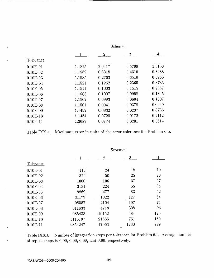
Tolerance

Scheme:

1 2 3 4

0.10E-01 1.1825 2.0417 0.5799 3.3158

0.10E-02 1.1569 0.6318 0.4310 0.8488

0.10E-03 1.1535 0.2763 0.3510 0.5983

0.10E-04 1.1521 0.1262 0.2365 0.3736

0.10E-05 1.1511 0.1003 0.1515 0.2587

0.10E-06 1.1505 0.1007 0.0958 0.1845

0.10E-07 1.1502 0.0993 0.0604 0.1307

0.10E-08 1.1501 0.0941 0.0378 0.0940

0.10E-09 1.1492 0.0832 0.0237 0.0736

0.10E-10 1.1454 0.0720 0.0172 0.2112

0.10E-11 1.3087 0.0774 0.0201 0.5614

MaximumTable IXX.a error in units of the error tolerance for Problem 6.b.

Tolerance

Scheme:

1 2 3 4

0.10E-01 113 24 18 19

0.10E-02 326 50 25 23

0.10E-03 1000 106 37 27

0.10E-04 3131 224 55 34

0.10E-05 9869 477 83 42

0.10E-06 31177 1022 127 54

0.10E-07 98557 2194 197 71

0.10E-08 311633 4718 308 93

0.10E-09 985438 10152 484 125

0.10E-10 3116197 21855 761 169

0.10E-11 9854247 47063 1200 229

Table IXX.b Number of integration steps per tolerance for

of repeat steps is 0.00, 0.09, 0.09, and 0.00, respectively.

Problem 6.b. Average number

NASA/TM--2000-209400 39

Numerical Results - Stiff Equations

In this section we briefly consider stiff equations. For a set of model problems we use

Problems 9 - 13 below.

Problem 9: (Enright and Pryce [33], Problem A3)

!Yl = -104yl + 100y2 - 10y3 + Y4

Y_ = -- 103 Y2 + 10y3 -- 10y4

!

Y3 -- --Y3 + 10y4

y_ = - 0.1 Y4

yl(0) = 1, y2(0) = 1, y3(0) = 1, y4(0) = 1, tend = 20

Problem 10: ([33], Problem B1)

!

Yl ---- -Yl + Y2

y_ = - 100yl -- Y2!

Y3 = --100y3 + Y4

/Y4 = -- 104y3 -- 100y4

yl(0) = 1, y2(0) = 0, y3(0) = 1, y4(0) : 0, ten d : 20

Problem 11: ([33], Problem D4)

y_ = -0.013yl - 1000yly3

!

Y2 = - 2500 Y2 Y3

y_ = - 0.013 Yl - 1000 Yl Y3 -- 2500 Y2 Y3

Yl(0) = 1, y2(0) = 1, y3(0) = 0, tend = 50

NASA/TM--2000-209400 40

Problem 12: (Robertson [34])

!

Yl = - 0.04 Yl + 104 Y2 Y3

y_ _-- 0.04yl - 104y2Y3-- 3"107y2

3 10 7 2Y3 " Y2

yl(0) : 1, y2(0) = 0, y3(0) = 0, tend = 40

Problem 13: ([33], Problem F3)

y_ = - 107 Y2 Yl + 10 Y3

!

Y2 = -- 107 Y2 Yl - 107 Y2 Y5 + 10y3 q- 10 Y4

Y3 = 107 Y2 Yl -- 1.001 • 104 Y3 q- 10-3 y4

!

Y4 : 104 Y3 -- 10.001 y4 q- 107 Y2 Y5

y_ = 10 Y4 -- 107 Y2 Y5

yl(O) : 4" 10 -6 , y2(O) = 1.10 -6 , y3(O) = O,

tend = 100

y4(0) : 0, y5(0) _-0

We integrated each system using Schemes 1 - 4, along with a trapezoidal extrapolation

scheme which we now introduce.

Let yT denote the trapezoidal solution (2.15), and let y!2) denote the degree-2 Taylor

series solution (3.14) with # = ½. One can show that the extrapolated solution

(2) T2_,_+1 + Y,+I (9.7)

Y_+I := 3

NASA/TM--2000-209400 41

is A-stable and fourth-order-accurate with truncation error

02f. ]h5 Of,,:,,, (02fn + fi,)f:[ (9.8)y(t,,+l)- y, +x - 2880 :"'' + 5- -y .. + 20,0to v ov 2 .

A variable stepsize for (9.7) can bc obtained using (7.1) together with the O(h 3) error

_ _ (2) I The above extrapolation with variable step implementationestimate % = [Yn+l u,_+l,.will be called Scheme 2T.

In integrating Problems 9 - 13, the parameters _, hf_t, and u, introduced in Section

7, were assigned default values of 0.9, 2.0, and 0.7, respectively, except for Scheme 1 where

was set to 0.7. Any deviation from these values is noted at the bottom of Tables XX

- XXIV. The local error estimate % was taken to be the largest absolute error in any

solution component. The initial stepsize was determined as in Section 7 (with appropriate

modifications for a system).

Tables XX - XXI demonstrate some degradation in the ability of Schemes 1 - 4 to

meet the error tolerance. Whether this holds in general for stiff problems requires further

investigation.

One also observes that the eighth-order-accurate Scheme 4 frequently required more

steps than some of the lower order schemes. This contrasts with the nonstiff results pre-

sented earlier, and illustrates the well known need for stiff solvers to be able to vary their

order.

Tolerance

Scheme:

1 2 2T 3 4

0.10E-01 0.1512 0.0485 0.0096 0.0326 0.3952

0.10E-02 0.2270 0.0628 0.0129 0.0332 1.0237

0.10E-03 0.3221 0.1356 0.0164 0.0339 2.1679

0.10E-04 0.3287 0.1016 0.0229 0.0393 2.8883

0.10E-05 0.3292 0.0450 0.0155 0.0488 6.2514

0.10E-06 0.3293 0.0453 0.0100 0.0695 4.1981

0.10E-07 0.3293 0.0455 0.0095 0.4929 6.7522

0.10E-08 0.3295 0.0443 0.0095 0.5759 5.6286

0.10E-09 0.3265 0.0327 0.0086 1.9309 6.1883

0.10E-10 0.4206 0.0176 0.0061 5.1021 9.4324

0.10E-11 1.4309 0.1217 0.3659 5.7487 5.8660

Table XX.a Maximum error in units of the error tolerance for Problem 9.

NASA/T ----2000-209400 42

Tolerance

Scheme:

1 2 2T 3 4

0.10E-01 121 34 34 24 31

0.10E-02 369 60 60 32 34

0.10E-03 1157 116 116 44 41

0.10E-04 3654 236 236 65 53

0.10E-05 11551 496 496 96 72

0.10E-06 36525 1055 1055 145 105

0.10E-07 115498 2259 2259 224 163

0.10E-08 365234 4851 4851 349 249

0.10E-09 1154967 10438 10438 547 406

0.10E-10 3652325 22473 22473 883 662

0.10E-11 11549662 48402 48402 1450 1119

Table XX.b Number of integration steps per error tolerance for Problem 9. Average

number of repeat steps is 0.18, 0.91, 1.18, 5.82, and 13.00, respectively. Changes to default

values: Scheme 3, u = 0.5; Scheme 4, hfact = 1.5, u = 0.5.

Tolerance

Scheme:

1 2 2T 3 4

0.10E-01 1.5593 2.8866 0.4222 0.7640 7.1984

0.10E-02 2.0085 3.0205 0.6115 0.8367 3.7537

0.10E-03 2.0902 2.1121 0.6816 0.5848 3.2502

0.10E-04 2.1074 3.2174 0.4245 0.9580 11.8994

0.10E-05 2.1121 3.3088 0.7441 0.6915 4.3284

0.10E-06 2.1134 2.2518 0.7997 0.5903 3.3849

0.10E-07 2.1141 2.8611 0.4129 0.8654 2.0479

0.10E-08 2.1142 0.9528 0.2677 0.3111 2.3132

0.10E-09 2.1166 0.4421 0.1545 0.2352 0.4552

0.10E-10 2.1143 0.2346 0.1879 0.2052 0.2391

0.10E-11 17.8417 0.4707 2.7374 0.1712 0.1882

Table XXI.a Maximum error in units of the error tolerance for Problem 10.

NASA/TM_2000-209400 43

Tolerance

Scheme:

1 2 2T 3 4

0.10E-01 712 135 142 73 44

0.10E-02 2219 299 304 118 70

0.10E-03 6992 642 648 192 105

0.10E-04 22082 1380 1389 307 147

0.10E-05 69805 2969 2978 486 211

0.10E-06 220720 6395 6397 766 297

0.10E-07 697952 13771 13775 1208 413

0.10E-08 2207094 29655 29656 1905 571

0.10E-09 6979416 63864 63864 3008 792

0.10E-10 22070843 137568 137569 4757 1092

0.10E-11 69794029 296360 296361 7528 1512

Table XXI.b Number of integration steps per error tolerance for Problem 10. Average

nunfl_er of repeat steps is 19.45, 26.64, 26.73, 19.18, and 10.00, respectively. Changes to

default values: Scheme 1, v = 0.5; Scheme 2, _ = 0.8; Scheme 2T, _ = 0.8; Scheme 3,

= 0.8; Scheme 4, _ = 0.8, u = 0.5.

Tolerance

Scheme:

1 2 2T 3 4

0.10E-01 23 13 13 15 40

0.10E-02 31 15 15 16 44

0.10E-03 56 17 17 17 46

0.10E-04 135 21 21 18 44

0.10E-05 387 29 29 19 46

0.10E-06 1187 46 46 22 48

0.10E-07 3720 83 83 26 51

0.10E-08 11734 164 164 32 54

0.10E-09 37081 337 337 43 77

0.10E-10 117237 710 710 60 117

0.10E-11 370738 1515 1515 89 189

Table XXII Number of integration steps per error tolerance for Problem 11. Average

number of repeat steps is 0.00, 1.45, 1.55, 0.09, and 10.36, respectively. Changes to default

values: Scheme 3, u = 0.5; Scheme 4, _ = 0.8, bract --- 1.5, u = 0.5.

NASA/TM--2000-209400 44

Tolerance

Scheme:

1 2 2T 3 4

0.10E-01 29 15 26 41 85

0.10E-02 48 91 22 43 79

0.10E-03 109 715 25 45 90

0.10E-04 303 41 41 47 73

0.10E-05 920 75 77 47 72

0.10E-06 2874 153 154 49 77

0.10E-07 9054 319 321 60 74

0.10E-08 28599 676 679 78 78

0.10E-09 90406 1448 1450 112 84

0.10E-10 285857 3108 3111 164 115

0.10E-11 903936 6686 6688 249 168

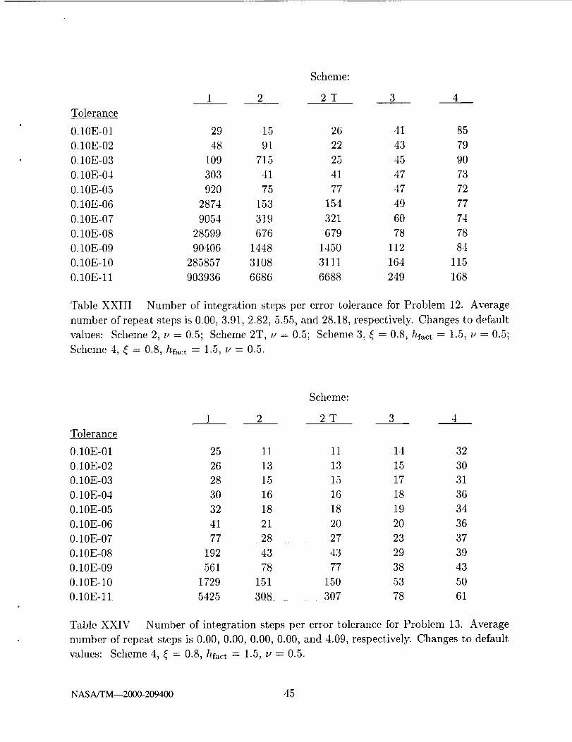
Table XXIII Number of integration steps per error tolerance for Problem 12. Average

number of repeat steps is 0.00, 3.91, 2.82, 5.55, and 28.18, respectively. Changes to default

values: Scheme 2, u = 0.5; Scheme 2T, u = 0.5; Scheme 3, _ = 0.8, hfact ---- 1.5, u -= 0.5;

Scheme 4, _ = 0.8, hfact = 1.5, u = 0.5.

Tolerance

Scheme:

1 2 2T 3 4

0.10E-01 25 11 11 14 32

0.10E-02 26 13 13 15 30

0.10E-03 28 15 15 17 31

0.10E-04 30 16 16 18 36

0.10E-05 32 18 18 19 34

0.10E-06 41 21 20 20 36

0.10E-07 77 28 27 23 37

0.10E-08 192 43 43 29 39

0.10E-09 561 78 77 38 43

0.10E-10 1729 151 150 53 50

0.10E-11 5425 308 307 78 61

Table XXIV Number of integration steps per error tolerance for Problem 13. Average

number of repeat steps is 0.00, 0.00, 0.00, 0.00, and 4.09, respectively. Changes to default

values: Scheme 4, _ = 0.8, hfact = 1.5, u = 0.5.

NASA/TM--2000-209400 45

Discussion and Conclusion

In this paper we have presented a new class of implicit Taylor series methods for

solving ODE initial value problems. Based on the results presented herein, we conclude

that the main advantages of implicit series methods are (i) ability to achieve high accuracy

while maintaining stability, (ii) robustness, (iii) simplicity, and (ix,) versatility (ability to

solve a wide range of problems).

However, implicit series methods suffer the disadvantage of being computationally

intensive. Table XXV summarizes the median number of Newton iterations per step for

tile results presented in the last ttiree sections. Tile Newton convergence criteria for these

results was that successive solution iterates differ by less than 10 -14 .

It is seen that a minimum of four Newton iterations are required per step - two

iterations for each independeut solution calculated. This means that, for a system of

equations, at least two L-U decompositions must be performed at each step. Consequently,

an implicit series method must be able to solve a given problem in relatively fewer steps

to be competitive with other methods. For most nonstiff problems, this implies the need

for a series with high order accuracy. For stiff problems, this implies the need to vary the

order of accuracy during the calculation.

We conclude with tile following remarks. First, for nonstiff problems, corrector itera-

tion is an attractive alternative to Newton iteration. It is easier to implement, requires less

derivative information, and for small error tolerances is often more computationally effi-

cient. It works especially well for small, uniform stepsizes. Second, for problems without

a singular point, Scheme 2T is preferred over Scheme 2. Although both schemes employ

a degree-two Taylor series, use the same local error estimate (to O(hr')), and generally

require the same number of marching steps, Scheme 2T can be programmed in real arith-

Inetic and is significantly faster as a result. Third, due to tile length of this paper, we

have not made any direct comparisons with other methods. Comparing the efficiency and

reliability of integration methods has practically become a specialty in itself, and requires

considerable care and discussion. The intent here is to present enough results to give some

idea of performance on a range of problems. The next step toward a full comparison with

other methods is to extend implicit series methods to become a variable order approach.

This is proposed as a future research topic. Fourth, and lastly, implicit Taylor series meth-

ods offer a unique combination of high accuracy, stability, robustness, and versatility. The

author is not aware of another existing method that can, without modification, solve both

regular ODE's and stiff systems, together with linear and nonlinear ODE's with a singular

point -- all with an arbitrarily high order of accuracy. With computer speed and memory

steadily increasing, algorithm features such as robustness, versatility, and ease of use are

becoming increasingly important. For this reason, implicit Taylor series methods merit

conSlderatl0n as a standard integration tool for solving ordinary differential equations.

NASA]TM--2000-209400 46

Problem:Scheme 1 2 3 4 5 6a 6b

1 4.00 5.00 4.00 5.00 4.92 4.00 4.00

2 4.00 5.97 4.12 5.73 5.73 4.00 4.00

3 4.00 7.72 4.33 7.94 6.90 4.00 4.00

4 4.00 7.84 4.81 8.56 7.52 4.00 4.00

9 t0 11 12 13

1 4.00 4.00 5.95 6.00 5.56

2 4.00 4.02 6.41 7.01 5.43

2T 4.00 4.02 5.82 6.00 5.35

3 4.02 4.15 9.78 13.65 6.35

4 4.08 4.18 17.08 26.57 10.56

Table XXV Median number of Newton iterations per timestep.

NASA/TM--2000-209400 47

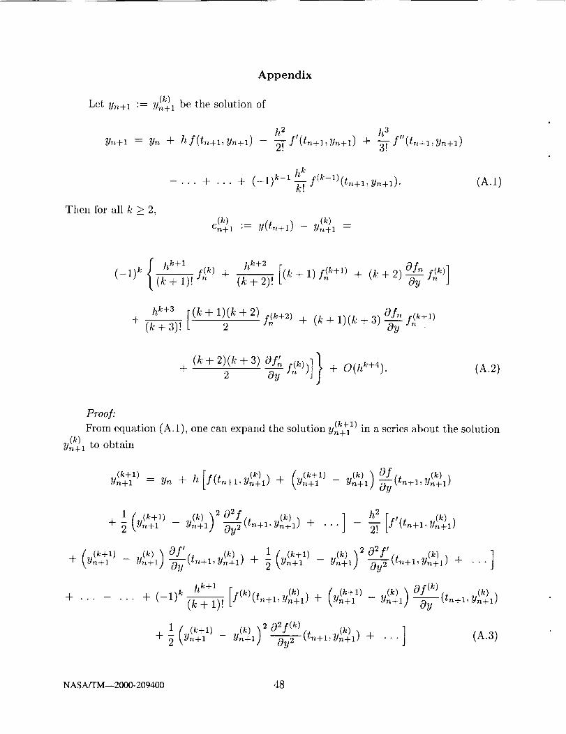
Let Yn+l

Yn+l =

Appendix

(k) be the solution of:= Yn+l

Yn + h,f(tn+l,Yn+l) h2 ha f"2! f'(tn+l,yn+l) + _ (t,,+l,yn+l)

... + ... + (-1) k-1 tzkk--( f(a-1)(tn+l,yr_+l).

Then for all k _> 2,

e(k) . (k)n+l := y(t,_+l) - =Yn+l

(A.1)

hk+l f(k) +(-1)a (k + 1)! hk+2 [(k+2)! (k+l) f(k+U + (k + 2) Of., f(k)]

Of,_ r(k+_)h k+3 (_ + 1)(k + 2) t.(k+2 ) + (k + 1)(k + 3) _+ (k + 3)! 2 _'_ _'_

+ (k+ 2)(k+ 3) of', ]}2 Oy f(k)) + O(hk+4).(A.2)

Proof:o (k+l)

From equation (A.1), one can expand the solution Yn+l in a series about the solution

b(k) to obtainn+l

---- -- Yn+l _yy Yn+l}tin+l/ + LYn+I (tn+l,

1 /' (k+l) q (k) ,_2 02f (tn+l, " (k),, ] h2 [ q (k))- Yn+l) + f'(tn+I,-_- 2 LYn+I Yn+i] _ " "" "_. Yn+l]

{ (k+l) ,(k) ,(k) _ [ (k+l, ,,(k) ) ___y2 (tn+l,y(k)+l) + ]+ LYn+I _n+l) Of' 1 2 02f '+ - , ...-- _n+l] 2 Yn+

+ ... - ... + (-1) k ha+l [f(a)(t,_+l(k+ 1)!

. (a) / (a+_),Yn+l) + [Yn+l --

b(k) _ Of (k) t, o (k)

(A.3)

NASA/TM--2000-209400 48

from which one gets

y(k+i)n+l -- Y,_ + h f(tn+l °,_,_+11(k)

h2 , A(k)2! f (t_+x, y,_+lJ

+ ... - ... + (-1) khk+l

(k+ 1)!

(_ (k+l) _ (k) '_ [h Of-_- kgn+l -- Yn+l) _ Yn+x)_y(tn+l " (k) ,

+ ... - ... + (-1) k

-_- ° . ,

f(k) (t,_+l," (k)Yn+l)

h 2 Of'

2_ Oy(tn+ i _ (k) xYn+l)

hk+ 1 Of(k)

(k + 1)! Oy

- _'n+l) _--fiy2t_-+l, vn+lJ

h 2 02f ' _ (k)

2! Oy 2 (tn+l,_n+11

... + (-1) khk+l 02f(k)

(k + 1)! Oy 2

-I- • • •

(A.4)

Now

y_ + hf(tn+_,_,_+_)

+ ... -- 3- (--1) k-1 hk"'" k!

from equation (A.1). Therefore (A.4) becomes

h 2

,t_n+l J2_

__ f(k_l)(t_+i,_ (k) _ (k)un+lz _ Yn+l (A.5)

_ ,(k) = (_l)kYn+l

h k+l _ (k)

(k + 1)! f(k)(tn+l' _]n+l)

(_ (k+_)+ \Un+I . (t_) _ [[hOf (tn+l, " (k)9n+lyn+ ) )

-_ • ° ° -- , • •

1 [ (k+i) _ (k) 'l+ 7 tyn+, -

-_ ° ° , -- , • •

(k+i)It follows from (A.6) that v_+i

one gets

h 2 Of'

2! Oy(tn+ 1'- (k) xYn+l)

(k) (i (A.6)+ (-1) k hk+l of(k)(t,,+l, un+lJj(k + 1)! Oy

2 [h 02f i, _ (k)'2y2 kVn+l _ Yn+l}

h 2 02f ' _ (k)

2! Oy _"(tn+l, Yn+l]

hk+ 1 02f(k) _ (k))]+ (-1)_ (k + 1)! Oy_ (t_+_,_+_

_- o ° •

-(_) is O(hk+l). Retaining terms through O(hk+3),-- 9n+l

NASA/TM--2000-209400 49

(k+l) (k) h k+_ . (k)

Yn+l - Yn+l = (-1) k (k+ 1)! f(k)(t'_+l'Y"+ll

/ (k+l) _(k) _ [ Of h 2 Of' ]+ _Y,,+I h (t,,.+1 I) + O(h3) (A.7)- Yn+I} _yy(tn+l _ (k) _ _(k), ten+l! 2 0 9 ,/Jn+

so that

(k) = _J'-l'k-- Yn+l

h k + 1

(k + 1)!(k) /f(k) (t,,+:, _+:)

/

Yn + 1 )1 - It =--(t,,+l, +oy" 20y

For sufficiently small h, one then obtains

(A.8)

y(k+l)n+l

(k) = ;;'-l'k-- _/n+I

hk+l

(k+ 1)! off(k)(t,,+ 1 ,(k) _ 1 + h =---(t,,+l, ° (k)"!In+ 1 ],Yn + 1 ] oy

+ he [ 0f(t'+lay ' y'+(k)1J'2 _ -21--Off(t"+"'OyYn+lJ](k),l } + O(hk+4). (A.9)

Now each term on the right hand side of (A.9) can be expanded in a series about (tn, yn),

so that

b(k+l) .(k) hk+l [ Of (k) / (k) Of(* k)

,,+I - Y,_+I = (-1) k (#T I-)! LA(k)+ h _ + ky_+1-y,,)

+2 Ot 2 + h [Yn+l- OtOy + -2 [Yn+l- Oy 2 + O(h 3) 1 + h O---y-

+ h202f.. / (k) Yn)02f_ h2" 0f,_,2 10_;1OtOy+ h t,_n+l- Oy_ + [(-0T; 2 0yJ + O(h_) (A.10)

For all k > 2, equation (3.8) shows that

h 2

_(k) hA + f', + o(h_)..Vn+l - Y_ = -_- (A.11)

Substituting (A.11) into (A.10) and simplifying, one finally obtains

_(k+_) ,(k) h_+I [ oA A(k)),,+,- _,,+i= (-_)_(i7_)!f'(_)+ h(z_(k+1)+

--t- -_-h'2 (f(k+2)_}_ 2 0fnf(k+l)oqy -Jr- --_y f(n k)) • (A.12)

NASA/TM--2000-209400 50

Since

_(k+l)_ _(k) Ak+l) (A.13)(k+l) _ (k) _ (k) y(tn+l) - Yn+l ) "m+l - %+1Y,,+I - _,_+1 = y(t,,+l) - _+1 - =

one obtains from (A.12)

en+l(k+l) en+l-(k) 1)k+l (/_TT)!hk+l [ _Of" f(k))- = (- f,?) + h +

Of', ]

h 2

Since n and h are both fixed, (A.14) is a linear difference equation on k. One can verify by

direct substitution that tile solution to the difference equation is given by (A.2), plus an

arbitrary constant which may be taken to be zero. Therefore (A.2) is valid for all k > 2.

References

1. J.R. Airey, "Emden Functions," British Association for the Advancement of Science

Mathematical Tables, Vol. II. B. A., London (1932).

2. J.C.P. Miller, "The Airy Integral," in British Association for the Advancement of

Science Mathematical Tables, Part-Vol. B. Cambridge Univ. Press, London and New

York (1946).

3. J.C.P. Miller, "Numerical Analysis, An Introduction" in The Numerical Solution of

Ordinary Differential Equations, (J. Walsh, ed.) Chapter 4, Academic Press, New

York and London (1966).

4. A. Gibbons, A program for the automatic integration of differential equations using

the method of Taylor series, Comput. or. 3, 108 (1960).

5. R.A. Moore, Interval Analysis, Prentice-Hall, Englewood Cliffs, New Jersey (1966).

6. J.A. Leavitt, Methods and applications of power series, Math. Comp. 20, 46 (1966).

7. V.S. Nikolaev, The solution of systems of ordinary differential equations by expansion

in power series on high speed computers, USSR Comp. Math. and Math. Phys. 5, 32

(1965).

8. D. Barton, I.M. Willers, and R.V.M. Zahar, The automatic solution of ordinary dif-

ferential equations by the method of Taylor series Comput. J. 14, 243 (1971).

9. D. Barton, I.M. Willers, and R.V.M. Zahar, Taylor series methods for ordinary differ-

ential equations- an evaluation, In Mathematical Software, John Rice (Ed.), Academic

Press, New York, 369 (1971).

NASA/TM--2000-209400 51

10. A.C. Norman, Expanding the solutions of implicit sets of ordinary differential equa-tions in power series, Comput. J. 19, 63 (1976).

11. (3. Kedem, Automatic differentiation of computer programs, A.C.M. Trans. Math.

Softw. 6, 150 (1980).

12. L.B. Rall, Automatic Differentiation: Techniques and Applications, in Lecture Notes

in Computer Science 120, Springer-Verlag, New York (1981).

13. Y.F. Chang, Automatic Solution of Differential Equations, in Constructive and Com-

putational Methods for Differential and Integral Equations, D.L. Colton and R.P.

Gilbert (Eds.). Lecture Notes in Mathematics 430, 61, Springer-Verlag, New York

(1974).

14. (3. Corliss and Y.F. Chang, Solving ordinary differential equations using Taylor Series,

A.C.M. Trans. Math. S@w. 8, 114 (1982).

15. D.H. Irvine and M.A. Savageau, Efficient solution of nonlinear ordinary differential

equations expressed in S-system canonical form, SIAM J. Numer. Anal. 27, 704

(1990).

16. M.A. Savageau and E.O. Volt, Recasting nonlinear differential equations as S-systems:

a canonical nonlinear form, Mathematical Biosciences 87, 83 (1987).

17. Y.F. Chang and (3. Corliss, Compiler for the solution ordinary differential equations

using Taylor series, Tech. Rep., Marquette Univ., Marquette, Wisconsin (1981).

18. Y.F. Chang, G. Corliss, and R. Morris, ATSMCC User Manual, Dep. of Mathemat-

ics, Statistics, and Computer Science Rep., Marquette Univ., Marquette, Wisconsin

(1979).

19. T.E. Hull, W.H. Enright, B.M. Fellen, and A.E. Sedgwick, Comparing numerical

methods for ordinary differential equations, SIAM J. Numer. Anal. 9, 603 (1972).

20. K. Kastlunger and G. Wanner, On Turan Type Implicit Runge-Kutta Methods, Com-

puting 9, 317-325 (1972).

21. L. Lapidus and J.H. Seinfeld, Numerical Solution of Ordinary Differential Equations,

Mathematics in Science and Engineering 74, 61, Academic Press, New York and

London (1971).

22. J.D. Lambert, Numerical Methods for Ordinary Differential Systems, 190, John Wiley

and Sons, Chichester (1991).

23. G. Dahlquist, A special stability problem for linear nmltistep methods, BIT 3, 27

(1963).

24. C.W. Gear, Numerical Initial Value Problems in Ordinary Differential Equations, 212,

Prentice-Hall, Inc., Englewood Cliffs, New Jersey (1971).

25. G. Dahlquist, Stability questions for some numerical methods for ordinary differential

equations, Proc. Symposia in Applied Mathematics 15, 147 (1963).

NASA/TM--2000-209400 52

26. B.L. Ehle, High order A-stable methodsfor the numericalsolution of systemsof D.E.'s,BIT S, 276 (1968).

27. H. Scholz, The examination of nonlinear stability and solvability of the algebraic

equations for the implicit Taylor series method, Appl. Num. Math. 28, 439 (1998).

28. E. Hairer, S.P. Norsett, and G. Wanner, Solving Ordinary Differential Equations I,

2nd Edition, Springer Series in Computational Mathematics, 168, Springer-Verlag,

New York (1987).

29. G. Corliss and D. Lowery, Choosing a stepsize for Taylor series methods for solving

ODE's, J. Cornp. A. Math. 3, 251 (1977).

30. K. Radhakrishnan and A.C. Hindmarsh, Description and Use of LSODE, the Liv-

errnore Solver for Ordinary Differential Equations, 62, NASA Reference Publication

1327, Lawrence Livermore National Laboratory Report UCRL-ID-113855 (1993).

31. A. Holubec and A.D. Stauffer, Efficient solution of differential equations by analytic

continuation, J. Phys. A. Math. Gcn. 18, 2141 (1985).

32. M. Haftel, R. Krivec, and V.B. Mandelzweig, Power series solution of coupled differ-

ential equations in one variable, J. Cornp. Phys. 123, 149 (1996).

33. W.H. Enright and J.D. Pryce, Two FORTRAN packages for assessing initial value

methods, ACM Transactions on Mathematical Software 13, 1 (1987).

34. H.H. Robertson, The solution of a set of reaction rate equations, in Numerical Anal-

ysis, 178, J. Walsh (ed.), Thompson Book Co., Washington (1967).

NASA/TM--2000-209400 53

' I ' I ' I ' I '

t-

Em

!1

>

3

-1

-3

Figure 1.a

Unstable

I t _ I t t

-8 -6 -4

u = Re(Xh)

Stability region for Euler's method.

I I ,

-2 0

NASA/TM--2000-209400 54

' I ' I ' I ' I '

c"

V

Em

II

>

3

-1

Figure 1.b

Unstable

-8 -6 -4 -2

u = Re.(;Lh)

Stability region for a degree-2 explicit Taylor series.

Stable

I

0

NASA/TM--2000-209400 55

' 1 ' I ' 1 ' I '

¢-

v

Em

II

>

3

1

-1

-3

_5 ...... L

-10

Figure 2

Unstable

I _ __1 , I

-8 -6 -4

u = Re(_h)

, L ,

Stability region for a degree-3 explicit Taylor series.

-2 0

NASA/TM--2000-209400 56

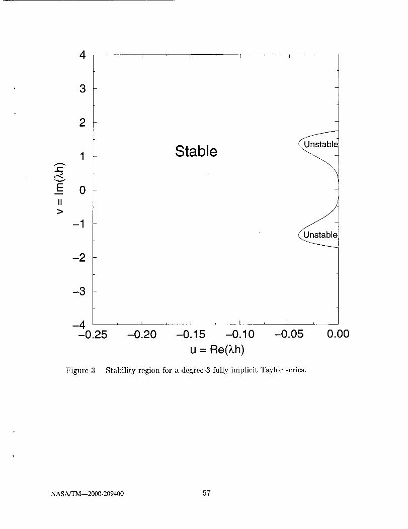
' I ' t ' I ' I '

t-

V

En

II

>

3

2

1

0

-1

-2

-3

Figure 3

Stable

I P I ,. I , I

-0.20 -0.15 -0.10 -0.05

u = Re(Xh)

Stability region for a degree-3 fully implicit Taylor series.

I

0.00

NASA/TM--2000-209400 57

_ 1 ' I _ I ' I '

c"

V

Em

II>

4

3

2

0

-1

-2

-3

-4

Figure 4.a

Stable

, L .... , I , t

-4 -3 -2

u = Re(;Lh)

1 1Stability region for a degree-3 Taylor series with # = _ + i _.

i r i

-1 0

NASA/TM--2000-209400 58

' I ' [ ' I

¢-

V

Em

II

>

4

3

2

0

-1

-2

-3

-4

Figure 4.b

' I *

Stable

, I , I , _1 , I ,

-4 -3 -2 -1

u = Re(;Lh)

1 i aStability region for a degree-3 Taylor series with # - 2 2

0

NASA/TM--2000-209400 59

' I ' [ ' I ' I '

¢..

V

Ei

II>

3

-1

Figure 5

Unstable

Stable

i 1

-8 -6 -4

u = Re(_h)

, I ,

Stability region for a degree-4 explicit Taylor series.

-2 0

NASA/TM--2000-209400 60

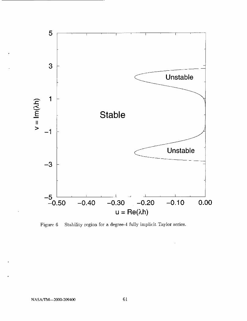
' I ' I ' I ' I '

¢-

v

Em

II

>

3

-1

-3

Stable

-0.40 -0.30

_- Unstable

Unstable

-0.20 -0.10 0.00

u = Re(;Lh)

Figure 6 Stability region for a degree-4 fully implicit Taylor series.

NASA/TM--2000-209400 61

..lC

V

Em

II>

6

4

2

0-

-2

-4

-6

Figure 7.a

Stable

I , I , I L I ,

-4 -3 -2 -1 0

u = Re(_,h)

1 1 7rStability region for a degree-4 Taylor series with it = _ + i _ tan --10"

NASA/TM--2000-209400 62

' I ' I ' I

c-

V

Em

II

>

6

4

2

0

-2

_-4

-6

Figure 7.b

' I '

Stable

I

-4 -3 -2 -1 0

u = Re(;Lh)

1 1Stability region for a degree-4 Taylor series with # = _ - i _ tan _.

NASA/TM--2000-209400 63

' I ' I ' 1 ' I '

c-

v

En

II

>

6

4

2

0

-2

-4

-6

Figure 7.c

I

Stable

t , I , I , I t

-4 -3 -2 -1 0

u = Re(Xh)

1 1 _.Stability region for a degree-4 Taylor series with # = _ + i _ tan

NASA/TM--2000-209400 64

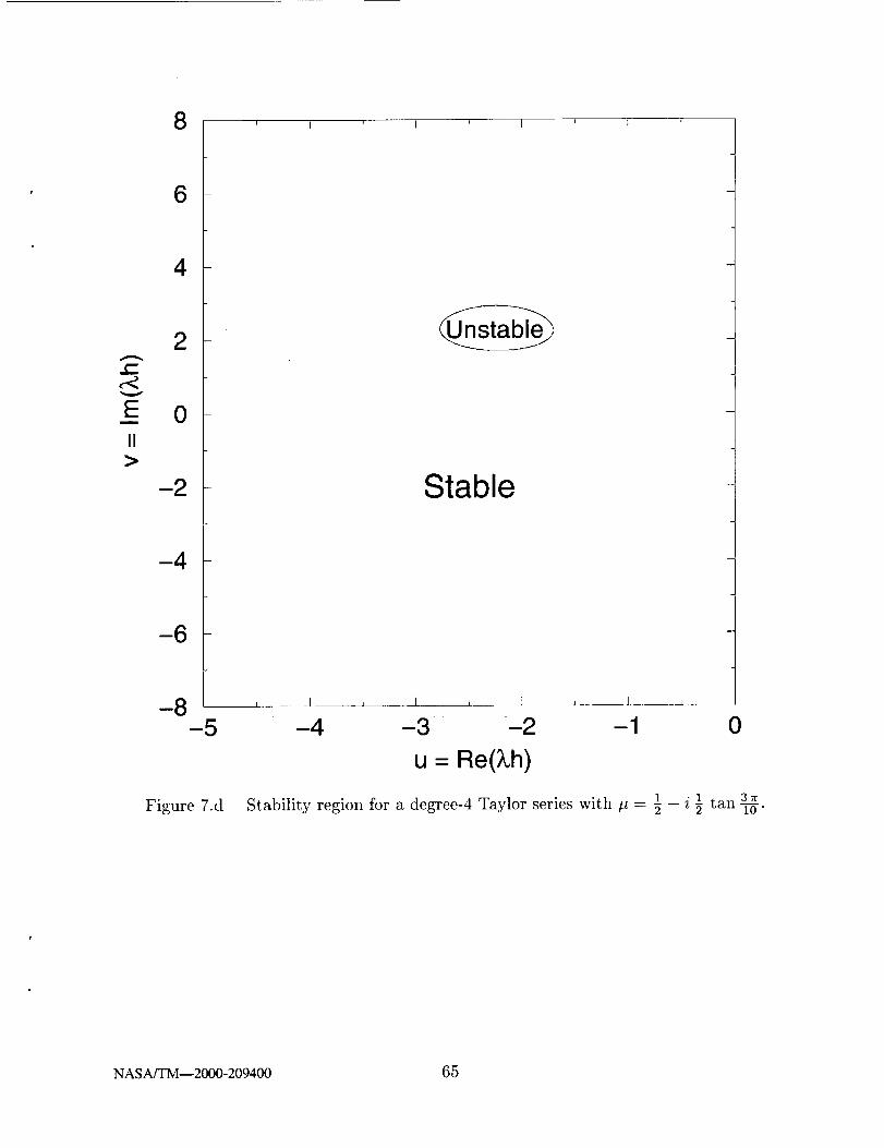
c-

V

Em

II

>

6

4

2

0

-2

-4

-6

Figure 7.d

Stable

, I , I , ] , l ,

-4 -3 -2 -1 0

u = Re(Xh)

t _ i ½ tan 3Stability region for a degree-4 Taylor series with tt = _ Tff"

NASA/TM--2000-209400 65

O

W

x

10-I

10-3

10-5

10-7

10 -9

10 -11

1 0 -13

I ! I I

Q---© CE

[] [] Trap/_ ±IMP

1 0 -15 J I I I

102 10° 10-2 10-4 10 -6 10-8

Stepsize h

Figure 8.a Reduction of error for Problem 1. Results are shown for the Centered Euler

Method, Trapezoidal Rule, and Implicit Midpoint Rule.

NASMTM--2000-209400 66

OL_

X

10 -1

10 -3

10-5

10 -7

10 -9

10 -11

1 0 -13

10 -15

I I I 1

I I I I

102 10° 10-2 10-4 10-6 10-8

Stepsize h

Figure 8.b Reduction of error for Problem 2. Results are shown for the Centered Euler

Method, Trapezoidal Rule, and Implicit Midpoint Rule.

NASA/TM--2000-209400 67

101 t I I I

0

LIJ

X

10-1

10 -3

10-5

10 -11

10 -13

1 0 -15 ,, I t 1 I

102 10° 10-2 10-4 10-8 10-8

Stepsize h

Figure 8.c Reduction of error for Problem 3. Results are shown for the Centered Euler

Method, Trapezoidal Rule, and Implicit Midpoint Rule.

NASA/TM--2000-209400 68

O

UJ

X

10-1

10 -3

10-5

10 -9

10 -11

1 0 -13

I I

10-15 I I _.

102 1O° 10-2 10-4 10-6 10-8

Stepsize h

Figure 8.d Reduction of error for Problem 4. Results are shown for the Centered Euler

Method, Trapezoidal Rule, and Implicit Midpoint Rule.

NASA/TM--2000-209400 69

10 -1

10 -3

10-5

0_- -7

"- 10UJX

1 0 -11

1 0 -13

1 i I I

0 OCE

[] [] Trap±IMP

10 -15 _ i r J I

102 10° 10-2 10-4 10-6 10.8

Stepsize h

Figure 8.e Reduction of error for Problem 5. Results are shown for the Centered Euler

Method, Trapezoidal Rule, and Implicit Midpoint Rule.

NASA/TM--2000-209400 70

v

E

00

Real(t)

1 v_Figure 9 Integration path for a degree-2 Taylor series with # = _ + i a •

NASA/TM--2000-209400 71

10 -2

10 .6

L_

0L-- -8

_- 10LU

x

:_ 10-1°

1 0 -12

1 0 -14

1 0 -16

Figure 10.a

__+ i,/52 6 "

I i I I

I I I t

102 1O° 10-2 10 -4 10-6 10-8

Stepsize h

Reduction of error for Problem 1 using a degree-2 Taylor series with # =

NASA/TM--2000-209400 72

10-1

10-3

10-5

0-7'- 10

UJ

X

1 0 -11

1 0 -13

1 0 -15

Figure 10.b

1 + i,/52 6 "

I I I I

I I l...... I

102 10° 10-2 10-4 10-6 10-8

Stepsize h

Reduction of error for Problem 2 using a degree-2 Taylor series with It =

NASA/TM--2000-209400 73

101 I I I I

10-1

10-3

10-_

0I,....I,=..,

w 10 -7X

10 -9

10 -11

10 -13

1 0 -15

Figure 10.c1 e52+i 6'

102 10° 10-2 10 -4 10-6 10-8

Stepsize h

Reduction of error for Problem 3 using a degree-2 Taylor series with # =

NASA/TM--2000-209400 74

10 -1 _

10 -3 _

10-5 _

10 -7 _

10-9 _

10-11

10 -13 _

1 0 -15

102

Figure lO.d

_+i 6"

I I I I

I I I I

1O° 10-2 10-4 10-8 10-8

Stepsize h

Reduction of error for Problem 4 using a degree-2 Taylor series with # =

NASA/TM--2000-209400 75

10 -1

10 -3

10-5

0I... -7

'- 10I.UX

10 .9

10 -11

1 0 -13

1 0 -15

Figure lO.e1 ,/5_+i 6 •

I I I i

I I I

102 10° 10-2 10-4 10 .6 10.8

Stepsize h

Reduction of error for Problem 5 using a degree-2 Taylor series with # --

NASA/TM--2000-209400 76

' t ' I ' I '

c-c,tV

Em

H

>

0.5

0

-1

-2

Figure 11

Stable

t I i 1 i I i

-1.5 -1 -0.5

u = Re(Xh)

Stability region for a degree-3 Taylor series with extrapolation.

0

NASA/TM--2000-209400 77

10o I I I I

0'L_

LUX

10 -2

10 -4

1 0 -10

1 0 -12

1 0 -14

0 O_tlS---EB #2l A extrap

]

1 0 -16 I , I 1 I

102 10° 10-2 10-4 10 -6 10-8

Stepsize h

Figure 12.a Reduction of error for Problem 1 using a degree-3 Taylor series with #1 = ½,1

#2 = _ + i ½, and with extrapolation.

NASA/TM--2000-209400 78

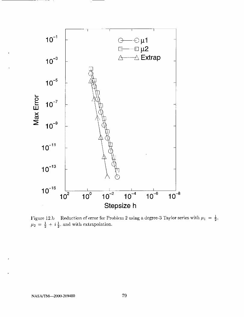
10-1

10 -3

10-5

0-7

'- 10UJ

X

10 -11

1 0 -13

I t I

O Opl[] [] p2

A A Extrap _

1 0 -15 I I J I

102 10° 10-2 10 -4 10-6 10-8

Stepsize h

Figure 12.b Reduction of error for Problem 2 using a degree-3 Taylor series with/,1

i 1 and with extrapolation.

1

NASA/TM--2000-209400 79

101 I I I I

O

I.U

X

10-1

10-5

10 -7

1 0 -11

1 0 -13

0 Ogl[] D g2

_ extrap

10 -15 .. I I I I

102 10° 10-2 10-4 10-6 10-8

Stepsize h

Figure 12.c Reduction of error for Problem 3 using a degree-3 Taylor series with tq = ½,1 1

#2 = _ + i 3, and with extrapolation.

NASA,rI'M--2000-209400 80

I I I I

OL_

UJ

X

10 -1

10 -3

10 -7

10 -9

10 -11

1 0 -13

©

[]

A

©gl

[] g2

A extrap

1 0 -15 ] _L i i P102 10 ° 10 -2 10 -4 10 -6 10 -8

Stepsize h

Figure 12.d Reduction of error for Problem 4 using a degree-3 Taylor series with #1

1 1 and with extrapolation.#2 = 7+i_,

i

NASA/TM--2000-209400 81

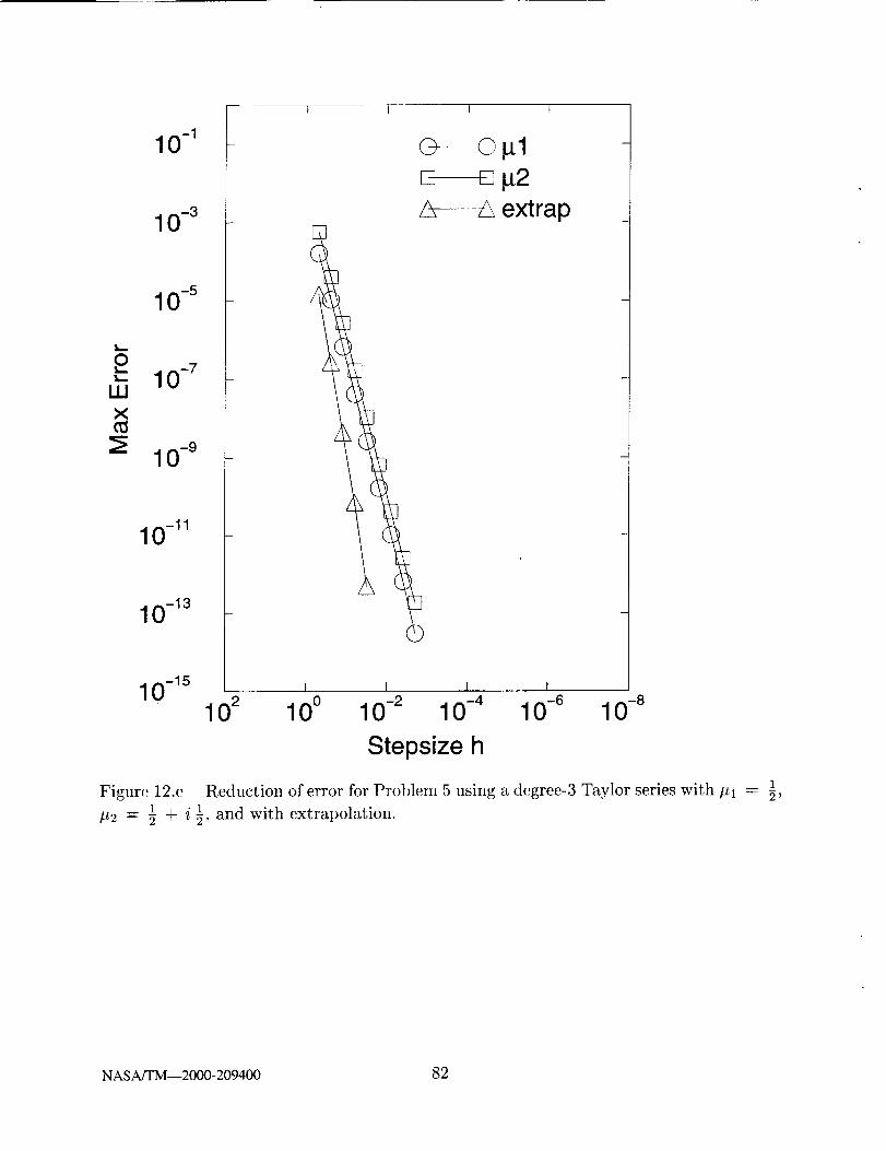
OI...

UJ

X

10 -I

10 -3

10-5

10 -9

10 -11

10 -13

10 -15

t I I t

_. -©gl

[] __g2....& extrap

I 1 1 I

102 10° 10-2 10-4 10-6 10-8

Stepsize h

Figure 12.e Reduction of error for Problem 5 using a degree-3 Taylor series with #1

1 1 and with extrapolation.IL2 -- 2 +i7'

1

NASA/TM--2000-209400 82

ml ' I ' I ' I ' t '

{-

v

Em

II

>

-2

-3

-4

-5

-6

-7

Figure 13

/Unstable Stable

Unstable

J

L I , I _ I , I z

-2 -1.5 -1 -0.5

u = Re(_h)

Stability region for a degree-4 Taylor series with extrapolation.

0

NASA/TM--2000-209400 83

10o I I

0

III

X

10 -2

10 -4

10-6

10 -8

1 0 -1°

1 0 -12

1 0 -14

0 0#1[] [] #2

extrap

1 0 -16 I I I t

102 10° 10-2 10-4 10-e 10-8

Stepsize h

Figure 14.a Reduction of error for Problem 1 using a degree-4 Taylor series with #1 =

1 1 3_ and with extrapolation.+ i_ tan_, #2 = ½ + i½ tan TS-,

NASA/TM--2000-209400 84

10o I I I I

0

UJX

10-2

10-4

10-6

1 0 -10

1 0 -12

1 0 -14

@-to gl[] [] g2A ± extrap

10-16 I L i I

102 10° 10-2 10-4 10-6 10-6

Stepsize h

Figure 14.b Reduction of error for Problem 2 using a degree-4 Taylor series with #1 =

1+il _i i_ tan _, #2 - _ + i _ tan -_, and with extrapolation.

NASA/TM--2000-209400 85

101 I I I I

0$-,

UJ

X

10 -1

10 -3

10-s

10-7

1 0 -11

1 0 -13

0 0#1_----_ #2/_ _ extrap

1 0 -15 I I _ I

102 10° 10-2 10-4 10-e 10-8

Stepsize h

Figure 14.c Reduction of error for Problem 3 using a degree-4 Taylor series with #a =

1 + i 1 1 1 3_ and with extrapolation._ tan_,p2 = _ + i_ tanT6-,

NASA/TM--2000-209400 86

O

UJ

X

10-1

10-5

10 -7

10 -9

10 -11

1 0 -13

1 0 -15

I I

I I I I

1 I

© ©gl -

g2A _ extrap _

102 10° 10-2 10-4 10-6 10-8

Stepsize h

Figure 14.d Reduction of error for Problem 4 using a degree-4 Taylor series with ttl =

-21+ i _1 tan 75,_ #2 = 71 + i ½ tan -i-if,anand with extrapolation.

NASA/TM--2000-209400 8 7

O

W

X

10-I

10 -3

10-5

10 -7

10 -11

1 0 -13

1 0 -15

I I

1

I I

[] [] #2

extrap

I l I I

102 10° 10-2 10-4 10-e 10-8

Stepsize h

Figure 14.e Reduction of error fox" Problem 5 using a degree-4 Taylor series with #t =1 l 7r I I 37r

+ i _ tan Y6, #2 = _ + i _ tan 5-_, and with extrapolation.

NASA]TM--2000-209400 88

¢-.

V

E

II

>

7

5

3

-1

-3

-5

-7

Figure 15.a

Stable

Unstable

q I , I J L

-3 -2 -1

u = Re(Xh)

Stability region for a degree-5 Taylor series with extrapolation.

0

NASA/TM--2000-209400 89

' I ' I ' I ' I ' I '

t-

V

E!1

>

-2

-4

-6

-8

Figure 15.b

Stable

o

Unstable 0

/Unstable

-5 -4 -3 -2 -1

u = Re(Xh)

Stability region for a degree-6 Taylor series with extrapolation.

0

NASA/TM--2000-209400 90

10 -2

10 -4

10 -6

0_,- -8'- 10UJX

1 0 -12

1 0 -14

1 0 -16 I

102 100

I I I I

© 0#1[] [] #2A _ extrap

iI 1 I

10-2 10-4 10-e 10-8

Stepsize h

Figure 16.a Reduction of error for Problem 1 using a degree-5 Taylor series with #1 = ½,1 1 7r

#2 = _ + i _ tan 3, and with extrapolation.

NASA/TM--2000-209400 91

10 -2

10 -4

10-8

10-8UJ

10 -_°

10 -12

1 0 -14

1 0 -16

I I I I

O----O gl

[] _ g2£, ± extrap _

1 I I I

102 10° 10-2 10-4 10-6 10-8

Stepsize h

Figure 16.b Reduction of error for Problem 1 using a degree-6 Taylor series with #1 =

1 1 1 3,_ and with extrapolation.2 + i_ tan_,p2 = _ + i½ tans-g,

NASA/TM--2000-209400 92

10-1

0-7

•- 10ILl

X

10 -9

10 -11

1 0 -13

1 0 -15

Figure 17.a1

= -2"

I I t

0 0 Prob. 6.a

[] [] Prob. 6.b

I I I L

102 10° 10-2 10.4 10.6 10-8

Stepsize h

Reduction of error for Problems 6.a,b using a degree-1 Taylor series with

NASA/TM--2000-209400 93

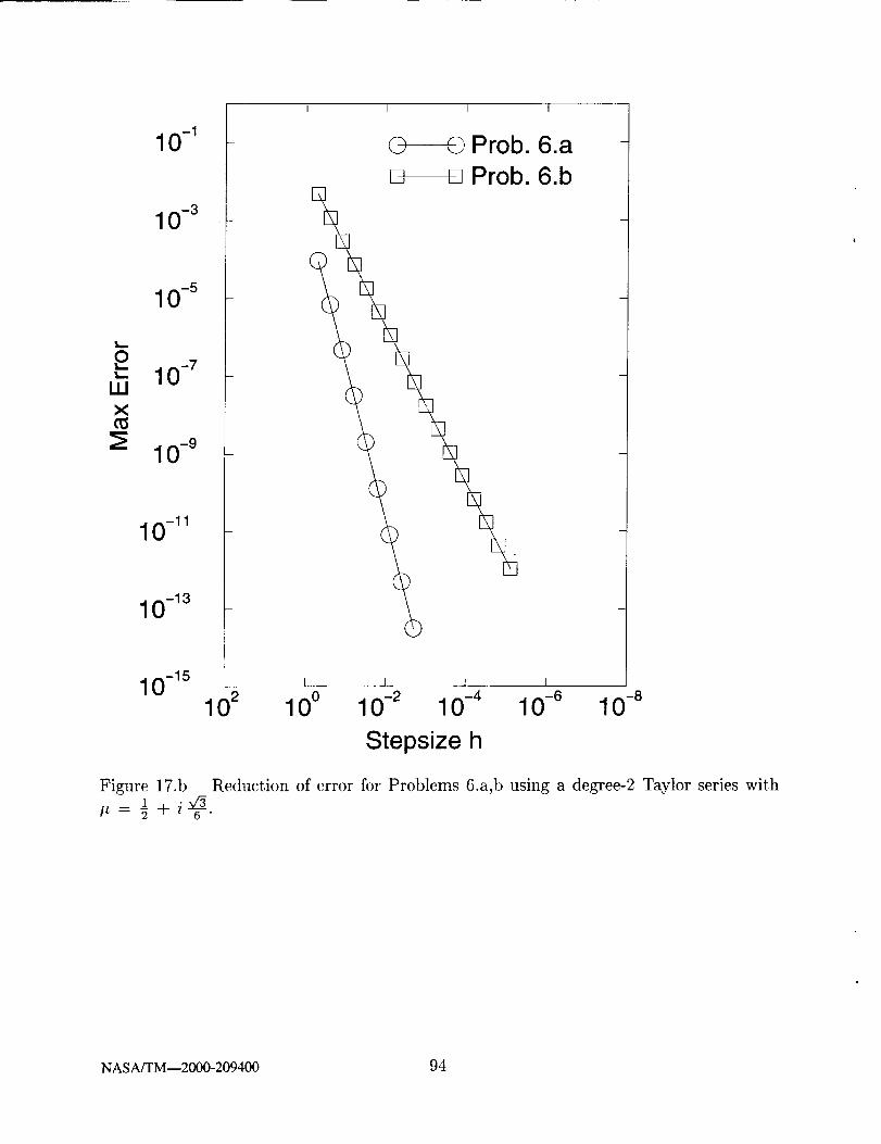
10-1

10-3

10-5

0I.. -7'-- 10

LM

X

10 -11

1 0 -13

F,

1 0 -15 i

102 10o

I I I

0 0 Prob. 6.a

[] [] Prob. 6.b

I 1 I

10.2 10 -4 10.6 10-8

Stepsize h

Figure 17.b Reduction of error for Problems 6.a,b using a degree-2 Taylor series with1 ,/5

It=-_+i 6 •

NASA/TM--2000-209400 94

10 -2

10 -4

10 -6

'L__

0• - -8•- 10

UJ

X

10-l°

1 0 -12

1 0 -14

I I I

© ©_tl -[] [] _2

/_ extrap _

1 0 -16 I I I L

102 10° 10-2 10-4 10-6 10-8

Stepsize h

Figure 17.c Reduction of error for Problem 6.a using a degree-3 Taylor series with #1 =

_,/_21 = _+i_,1 1 and with extrapolation.

NASA/TM--2000-209400 95

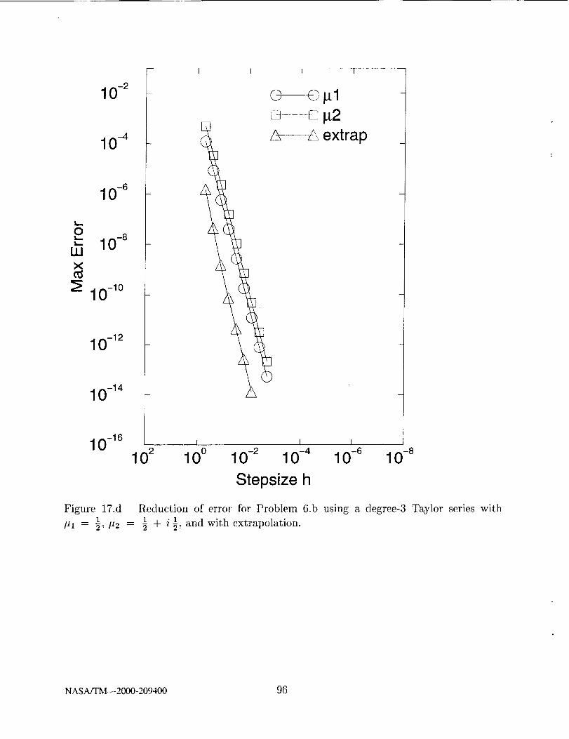
10 -2

10 -4

10-6

0L_ -8

•- 10IJ.I

X

10-l°

1 0 -12

1 0 -14

I I I I

© ©_1

[] [] _2A ± extrap

1 0 -16 I I I I

102 10 ° 10-2 10-4 10-e 10-8

Stepsize h

Figure 17.d Reduction of error for Problem 6.b using a degree-3 Taylor series with1 i

#1 = ½, #2 = g + i_, and with extrapolation.

NASA/TM--2000-209400 96

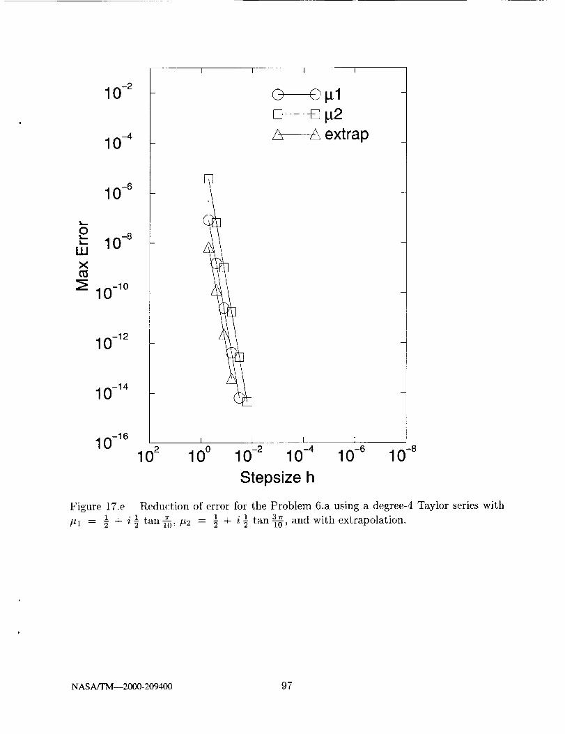
10 -2

10 -4

10 -6

0-8'.- 10

LUX

10-l°

1 0 -12

1 0 -14

I I I I

© ©gl

/_ ± extrap

1 0 -16 I I i

102 10° 10-2 10-4 10-6 10-8

Stepsize h

Figure 17.e Reduction of error for the Problem 6.a using a degree-4 Taylor series with

1 + i 1 _ 1 1 3,_ and with extrapolation.#1 = 7 _ tan 75,#2 = _ + i_ tan-F0-,

NASA/TM--2000-209400 97

10 -2

10 -4

10 -6

0I,- -8

•- 10ILl

X

10-l°

1 0 -12

1 0 -14

1 0 -16

I I I

© ©pl

[] [] p2& ± extrap

I l I I

102 10° 10-2 10-4 10-6 10-8

Stepsize h

Figure 17.f Reduction of error for Problem 6.b using a degree-4 Taylor series with #1 =

1 + i_1 tany6,_ #2 ---- _l + i½ tany6-,3_ and with extrapolation.

NASA/TM--2000-209400 98

10 -1

10 -3

10-5

0-7

'- 10UJ

X

10-9

10 -11

1 0 -13

1 0 -15

Figure 18.a

I I I I

I I I I

102 1O° 10-2 10-4 10-6 10 -8

Stepsize h

1Reduction of error for Problem 7 using a degree-1 Taylor series with p = 7.

NASA/TM--2000-209400 99

10 -2

10 -4

10 -6

0L --8'.- 10

U.i

X

10-l°

1 0 -12

1 0 -14

1 0 -16

Figure 18.b

1+i_2 6 "

t I I I

t I I I

102 10° 10-2 10-4 10 -6 10-8

Stepsize h

Reduction of error for Problem 7 using a degree-2 Taylor series with # =

NASAJTM--2000-209400 100

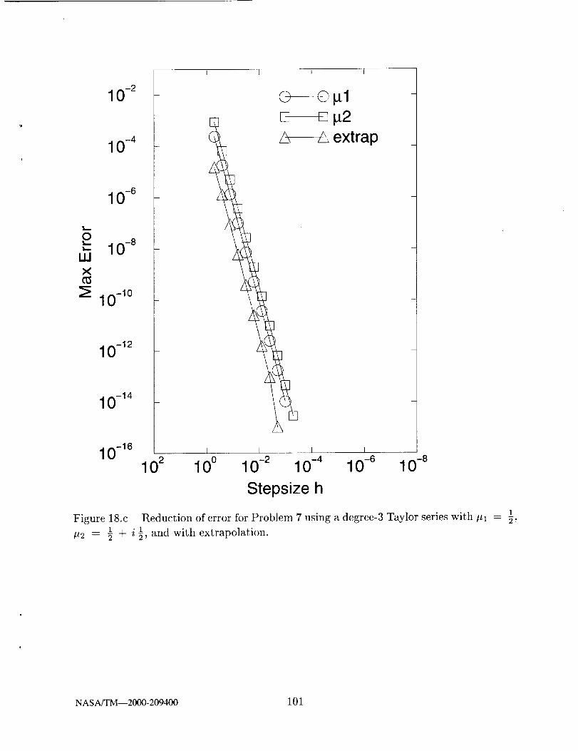
10 -2

10 -4

10 -6

0_,- -8'-- 10

UJ

X

10-l°

1 0 -12

1 0 -14

10 -16

I I I

0 0#1[] [] #2A & extrap

I I I I

102 1O° 10-2 10-4 10-8 10-8

Stepsize h

1Figure 18.c Reduction of error for Problem 7 using a degree-3 Taylor series with #1 = 5,

1#2 = _ + i ½, and with extrapolation.

NASA/TM--2000-209400 101

10 -2

10-4

0-8•" 1ILl

10-l°

1 0 -12

1 0 -14

1 0 -16

I I I I

Q----C_ _tl[] [] #2

/_ ± extrap

102 10 ° 10-2 10 -4 10-6 10 -8

Stepsize h

Figure 18.d

l+ii _ tan _, P2

Reduction of error for Problem 7 using a degree-4 Taylor series with #l =1 1 37r

= _ + i _ tan Tff, and with extrapolation.

NASA/TM--2000-209400 102

10 -1

10 -3

10-5

0•.,.. -7

'-- 10UJ

X

10 .9

1 0 -11

1 0 -13

1 0 -15

Figure 19.a]

#= _.

I I I

0 0 Prob. 8.a[] [] Prob. 8.b

1 I I 1

102 10° 10.2 10-4 10-e 10.8

Stepsize h

Reduction of error for Problems 8.a,b using a degree-1 Taylor series with

NASA/TM--2000-209400 103

10 -1

10 -3

10 -5

,o O-7'- 1LUX

10-9

10 -11

10 -13

I I I

0 0 Prob. 8.a

[] [] Prob. 8.b

rh

10-15 _ , _ J102 10° 10-2 10-4 10-6

Stepsize h

Figure i9.b Reduction of error for Problems 8.a,b using a degree-2 Taylor series with1 ,/5

#-----_+i 6 .

NASA/TM--2000-209400 104

I I

O

W

X

10-I

10-3

10-5

10-7

1 0 -11

1 0 -13

10-15 I I I 1

102 1O° 10-2 10-4 10-6 10-8

Stepsize h

Figure 19.c Reduction of error for Problem 8.a using a degree-3 Taylor series with #1 =1 1 17, #2 = 7 + i 7, and with extrapolation.

NASA/TM--2000-209400 105

I0-I

1 0 -3 -

10-5 _

o-7

'- 10IJJX

10-9

10-11

10 -13 _

1 0 -15 .....

102

Figure 19.d1

I I I I

0-- .....C_#1 -

[] [] #2/_ _ extrap _

I I 1 I

1O° 10-2 10-4 10 -6 10-8

Stepsize h

Reduction of error for Problem 8.b using a degree-3 Taylor series with1 1

+ i _, and with extrapolation.

NASA/TM--2000-209400 106

0

UJ

X

10-1

10-3

10-5

10 -7

1 0 -11

1 0 -13

I I t I

© ©gl_---_ g2/_ ± extrap

10-15 I I [ I

102 1O° 10-2 10-4 10-8 10-8

Stepsize h

Figure 19.e Reduction of error for Problem 8.a using a degree-4 Taylor series with #1 =

1 _t_ il _ 1 1 3_r_ tan _, P2 -- _ + i _ tan 75, and with extrapolation.

NASA/TM--2000-209400 107

10-I

10 -3

10-5

0II-- -7

•- 10LIJX

10-9

10 -11

1 0 -13

I I I I

© ©pl[] [] p2

A & extrap

10 -15 i I I I

102 10° 10-2 10-4 10-e 10-8

Stepsize h

Figure 19.f Reduction of error for Problem 8.b using a degree-4 Taylor series with gl -

1 1 ] 3_ and with extrapolation.+ i_ tan_4,#2 = _ + i½ tany_-,

NASA/TM--2000-209400 108

Form ApprovedREPORT DOCUMENTATION PAGE

OMB No. 0704-0188

Public reporting burden for this collection of information is estimated to average 1 hour per response, including the time for rewewing insiructions, searching existing data sources,

gathering and maintaining the data needed, and completing and reviewing the collection of information. Send comments regarding this burden estimate or any other aspect of this

collection of information, including suggestions for reducing this burden, to Washington Headquarters Services, Directorate for Information Operations and Reports, 1215 Jefferson

Davis Highway, Suite 1204, Arlington, VA 22202-4302, and to the Office of Management and Budget, Paperwork Reduction Project (0704-018B), Washington, DC 20503.

1. AGENCY USE ONLY (Leave blank) 2. REPORT DATE 3. REPORTTYPE AND DATES COVEREDMarch 2000 Technical Memorandum

4. TITLE AND SUBTITLE

Solving ODE Initial Value Problems With Implicit Taylor Series Methods

6. AUTHOR(S)

James R. Scott

7. PERFORMING (_RGANIZAT1ON NAME(S) AND ADDRESS(ES)

National Aeronautics and Space Administration

John H. Glenn Research Center at Lewis Field

Cleveland, Ohio 44135-3191

9. SPONSORII_IG/MONITORING AGENCY NAME(S) AND ADDRESS(ES)

National Aeronautics and Space Administration

Washington, DC 20546-0001

5. FUNDING NUMBERS

WU-522-81-11-00

8. PERFORMING ORGANIZATIONREPORT NUMBER

E-11836

10. SPONSORING/MONITORINGAGENCY REPORT NUMBER

NASA TM--2000-209400

11. SUPPLEMENTARY NOTES

Responsible person, James R. Scott, organization code 5940, (216) 433-5863.

12a. DISTI_i'BUTION/AVAILABtLITY STATEMENT

Unclassified - Unlimited

Subject Category: 64 Distribution: Nonstandard

This publication is available from the NASA Center for AeroSpace Information. (301) 621-0390.

12b. DISTRIBUTION CODE

13. ABSTRACT (Maximum 200 words)

In this paper we introduce a new class of numerical methods for integrating ODE initial value problems. Specifically, we

propose an extension of the Taylor series method which significantly improves its accuracy and stability while also

increasing its range of applicability. To advance the solution from t n to tn+ 1, we expand a series about the intermediate

point tn+p:= t n + ].lh, where h is the stepsize and/.t is an arbitrary parameter called an expansion coefficient. We showthat, in general, a Taylor series of degree k has exactly k expansion coefficients which raise its order of accuracy. The

accuracy is raised by one order if k is odd, and by two orders if k is even. In addition, if k is three or greater, local

extrapolation can be used to raise the accuracy two additional orders. We also examine stability for the problem y" = _y,

Re (_.) < 0, and identify several A-stable schemes. Numerical results are presented for both fixed and variable stepsizes. It

is shown that implicit Taylor series methods provide an effective integration tool for most problems, including stiff

systems and ODE's with a singular point.

14. SUBJECT TERMS

Taylor series; Implicit, Ordinary differential equation; ODE; Initial value problem; Time marching;

Numerical integration; Systems of equations; Stiff equations; Singular initial value problem

17. SECURITY CLASSIFICATIONOF REPORT

Unclassified

NSN 7540-01-280-5500

18. SECURITY CLASSIFICATIONOF THIS PAGE

Unclassified

19. SECURITY CLASSIFICATIONOF ABSTRACT

Unclassified

15. NUMBER OF PAGES

11416. PRICE CODE

A%20. LIMITATION OF ABSTRACT

i..

Standard Form 298 (Rev. 2-89)Prescribed by ANSI Std. Z39-18

298-102