Solving a Large-Scale Energy Management Problem With ... · Reviewer: Prof. Dr. rer. nat. Dorothea Wagner Advisors: Dipl.-Math. Reinhard Bauer Dr.-Ing. Andreas Cardeneo Dipl.-Inform

Solving a Large-ScaleEnergy Management Problem

with Varied Constraints

Diploma Thesis of

Felix Brandt

At the Department of InformaticsInstitute of Theoretical Informatics

Reviewer: Prof. Dr. rer. nat. Dorothea WagnerAdvisors: Dipl.-Math. Reinhard Bauer

Dr.-Ing. Andreas CardeneoDipl.-Inform. Markus Völker

Time Period: 9th February 2010 – 6th August 2010

www.kit.eduKIT – University of the State of Baden-Wuerttemberg and National Laboratory of the Helmholtz Association

Zusammenfassung (German Summary)

Diese Arbeit beschaftigt sich mit dem Problem der Wartungs- und Produktionsplanungeines großen konventionellen Kraftwerksparks unter Berucksichtigung vielfaltiger Nebenbe-dingungen und Unsicherheit uber einen Zeitraum von bis zu 5 Jahren. Die Aufgabenstel-lung entstammt dem ROADEF/EURO Challenge 2010, einem Wettbewerb der gemein-sam von der franzosischen Organisation fur Operations Research und Decision Support(ROADEF) und der Europaischen Organisation fur Operations Research (EURO) ausge-schrieben wurde. Das im Wettbewerb verwendete Modell und die zur Verfugung gestelltenDatensatze stammen vom großten Franzosischen Energieversorger Electricite de France(EDF). Da diese Arbeit erst nach der Vorrunde des Wettbewerbs begonnen wurde, konn-ten wir nicht mehr daran teilnehmen.

Das Modell unterscheidet zwei Typen von Kraftwerken, eine allgemein gehaltene Klasseetwa fur Kohle- und Gaskraftwerke oder Energieimporte und -exporte sowie eine Klassedetaillierter modellierter Kernkraftwerke. Die Aufgabenstellung enthalt drei voneinanderabhangige Teilprobleme. Erstens die Erstellung eines zulassigen Wartungsplans fur dieKernkraftwerke, das heißt die Festlegung von Zeitraumen, in denen die Kraftwerke vomNetz getrennt sind und gewartet werden. Die Wartungsplane mussen eine Reihe von be-reits mathematisch formulierten Bedingungen einhalten um unter anderem logistisch undpersonell durchfuhrbar zu sein, gesetzlichen Vorgaben zu genugen und die Netzstabilitatnicht zu beeintrachtigen. Das zweite Teilproblem ist die Erzeugung von Produktionspla-nen fur alle Kraftwerke unter verschiedenen Angebots- und Nachfrageszenarien. Aus denBrennstoffvorraten der Kernkraftwerke ergeben sich weitere Einschrankungen in den Pro-duktionsplanen. Die Festlegung der nachzufullenden Brennstoffmenge bildet das dritteTeilproblem, da das Auffullen nur wahrend einer Wartung durchgefuhrt werden kann. Dasubergeordnete Ziel ist die Minimierung der gesamten Produktionskosten.

Zu Beginn entwickeln wir zwei untere Schranken, welche wir in unserer Losung gewinnbrin-gend einsetzen. Wir losen das Problem in zwei Schritten. In einem ersten Schritt erzeugenwir einen gultigen Wartungsplan mit Methoden der Constraint Programmierung unterVerwendung des Open-Source Frameworks Gecode. Dabei erweitern wir das Modell umzusatzliche Bedingungen, welche die Losbarkeit der verbleibenden Teilprobleme sicherstel-len. Anschließend verwenden wir eine Weiterentwicklung einer der erwahnten Schranken,um mittels einer einfachen Greedy-Heuristik die Produktions- und Bevorratungsplane zuerstellen.

Im weiteren Verlauf der Arbeit entwickeln wir Techniken um unsere Ergebnisse zu verbes-sern. Ein erfolgreicher, randomisierter Ansatz betrachtet die Entwicklung der durch eineWartung verursachten Mehrkosten und bevorzugt gunstige Wartungszeitpunkte. Weiter-hin fuhren wir eine neue Bedingung ein, welche den Suchraum des Problems auf gunstigeWartungsplane beschrankt. Außerdem entwickeln wir eine Bevorratungsstrategie, welcheden erwarteten Profit in Relation zum Brennstoffvorrat setzt.

Abschließend vergleichen wir unsere Losungen der zur Verfugung gestellten Datensatzemit den besten bekannten Losungen der Wettbewerbsteilnehmer. Unser Ansatz erreicht

iii

iv

fur alle Datensatze gute Ergebnisse und entsprache einem 2. Platz unter den 21 Finalistendes Wettbewerbs.

iv

Selbstandigkeitserklarung

Hiermit versichere ich, dass ich die vorliegende Arbeit selbstandig angefertigt habe undnur die angegebenen Hilfsmittel und Quellen verwendet wurden.

Karlsruhe, den 06. August 2010

Unterschrift: .........................................

v

vi

vi

Acknowledgements

First of all, I want to thank Prof. Wagner for the opportunity to write my thesis ather institute about my self-chosen and not so common topic. Special thanks go to myadvisors (in alphabetical order) Reinhard Bauer, for his constant support over the lastmonths, his excellent guidance and his mathematical point of view, Andreas Cardeneo, forhis cooperation and especially for pointing me to the topic, and Markus Volker, for hisinsights to Gecode and lots of proofreading.

Finally, I would like to thank all of the other proofreaders of this thesis.

vii

Contents

1 Introduction 11.1 Related Work . . . . . . . . . . . . . . . . . . . . . . . . . . . . . . . . . . . 21.2 Overview . . . . . . . . . . . . . . . . . . . . . . . . . . . . . . . . . . . . . 2

2 Fundamentals 52.1 Constraint Programming . . . . . . . . . . . . . . . . . . . . . . . . . . . . . 52.2 Graphs and Networks . . . . . . . . . . . . . . . . . . . . . . . . . . . . . . 10

3 Problem Statement 133.1 Introduction . . . . . . . . . . . . . . . . . . . . . . . . . . . . . . . . . . . . 133.2 General Definitions . . . . . . . . . . . . . . . . . . . . . . . . . . . . . . . . 153.3 Constraints . . . . . . . . . . . . . . . . . . . . . . . . . . . . . . . . . . . . 183.4 Objective Function . . . . . . . . . . . . . . . . . . . . . . . . . . . . . . . . 23

4 Lower Bounds 254.1 Type-2 Power Plant Unit Production Cost . . . . . . . . . . . . . . . . . . . 254.2 An Auction-Based Lower Bound . . . . . . . . . . . . . . . . . . . . . . . . 294.3 A Flow-Based Lower Bound . . . . . . . . . . . . . . . . . . . . . . . . . . . 314.4 Evaluation . . . . . . . . . . . . . . . . . . . . . . . . . . . . . . . . . . . . . 41

5 Basic Solution 435.1 Outage Scheduling . . . . . . . . . . . . . . . . . . . . . . . . . . . . . . . . 435.2 Production Assignment . . . . . . . . . . . . . . . . . . . . . . . . . . . . . 575.3 Evaluation . . . . . . . . . . . . . . . . . . . . . . . . . . . . . . . . . . . . . 60

6 Optimization 656.1 Incremental Cost Branching . . . . . . . . . . . . . . . . . . . . . . . . . . . 656.2 Decremental Cost Branching . . . . . . . . . . . . . . . . . . . . . . . . . . 716.3 Sweep Margin Branching . . . . . . . . . . . . . . . . . . . . . . . . . . . . . 726.4 Online Propagator . . . . . . . . . . . . . . . . . . . . . . . . . . . . . . . . 736.5 Residual Fuel Penalty . . . . . . . . . . . . . . . . . . . . . . . . . . . . . . 756.6 Tuning Fuel Levels . . . . . . . . . . . . . . . . . . . . . . . . . . . . . . . . 76

7 Evaluation 817.1 Implementation and Testing Environment . . . . . . . . . . . . . . . . . . . 817.2 Provided Datasets . . . . . . . . . . . . . . . . . . . . . . . . . . . . . . . . 817.3 Evolution of Results . . . . . . . . . . . . . . . . . . . . . . . . . . . . . . . 837.4 Best Solutions . . . . . . . . . . . . . . . . . . . . . . . . . . . . . . . . . . . 83

8 Conclusion 87

List of Figures 89

ix

x Contents

List of Tables 91

List of Algorithms 93

Bibliography 95

x

1. Introduction

Electric energy is an essential resource in today’s life. No matter if we make our first cupof coffee or tea in the morning or run a multi-million euro business, all the time we relyon a secure and inexpensive supply of electricity. In this work we take the perspectiveof a large utility company, tackling their problems in modeling and planning productionassets, i.e., a multitude of power plants. Our goal is to fulfill the respective demand ofenergy over a time horizon of several years, with respect to the total operating cost of allmachinery.

Determining optimal maintenance schedules and production plans is not easy because ofthe number of alternatives to assess. As the exact electricity demand of each forthcomingday is unknown and depends on a large variety of factors (season, weather, holidays,etc.), this leads to the need of multiple uncertainty scenarios. Additionally, the increasingproportion of renewable energies in today’s energy mix makes things more complicated foran utility company, because it has to feed the energy of third-party solar or wind powerplants into its electricity networks and regulate its own power plants accordingly.

The problem discussed in this thesis was proposed by the ROADEF/EURO Challenge2010 [PGJ+], a competition announced by the French Operational Research and DecisionSupport Society (ROADEF) and the European Operational Research Society (EURO).The model has been developed by the French utility company Electricite de France (EDF).Since we started this work shortly after the challenge’s submission deadline for the qual-ification round passed, we could not take part in the competition. Nevertheless, we willcompare our results with the best results obtained by the participants of the challenge.

The examined problem comprises three fields of optimization: maintenance scheduling,production planning and determining refueling amounts. It is a tactical model, neitherconsidering short-term operational restrictions (like intraday load following) nor containingstrategic decisions (like adding new power plants). However, the proposed model allowsa generic formulation of other concerns like electricity network stability, safety consider-ations, availability of staff and tools, as well as legal restrictions. All of these limitationscan be expressed as mathematical constraints.

Our solution combines a constraint programming formulation of the problem with severalheuristics. We decompose the problem and develop different solution strategies rangingfrom very simple approaches up to sophisticated ones, which are driven by lower boundswe develop. Additionally, we present optimization techniques to improve our obtainedresults.

1

2 1. Introduction

Along with the presented solution methods we show our experimental results. All con-sidered problem instances are provided by the competition and are extracted from realworld data. Our solution performs competitive and provides good results for all proposedinstances.

One will notice the small differences between trivial and the best known solutions. But,as fuel cost is a major cost component in the power industry, it is worth optimizing alongthis edge. In the end, improving a solution by 0.1% is equivalent to saving several millionsof euros per year in operating cost.

1.1 Related Work

To the best of our knowledge, no work has been published yet that addresses the givenmodel. A former model proposed by EDF, comprising a subset of constraints and onlyconsidering maintenance scheduling, was solved by a combination of constraint program-ming and local search [KPB06]. While both models only accept solutions that fulfill allof the problem’s constraints, we note that most other models from the literature employpenalties if constraints are violated, rather than looking for exact solutions.

Nevertheless, there exists a vast amount of literature concerning production planning ofpower generating facilities. Different models have been proposed that track either main-tenance scheduling [FMS08],[SN91] or production planning [NKT00],[DR97]. A moregeneral problem addressed frequently in the literature is the unit commitment problem[Pad04],[FKL96],[SK98]. When applied to power systems the objective usually is to findlow-cost short-term (typically between 24 and 168 hours) production plans.

For a general introduction to solving combinatorial problems we refer to comprehensive lit-erature about combinatorial optimizations [NW88], networks and network flows [AMO93],and algorithms and data structures [CLRS01]. Methods which have successfully been ap-plied to power generation scheduling include genetic algorithms, ant colony search, tabusearch and simulated annealing [LES07]. A detailed introduction to different types andfeatures of power plants can be found in [WW96].

1.2 Overview

In the following we briefly outline the structure of this thesis:

Chapter 2 provides background knowledge of the main concepts of our solution and settlessome basic notation. It starts with a short introduction to constraint programmingand describes Gecode, the constraint programming toolkit that we use to solve partsof the problem. The chapter concludes with some basic definitions from the field ofgraph theory.

Chapter 3 gives an extensive introduction to the topic posed by the ROADEF/EUROChallenge 2010. After a first high-level presentation of the problem, we settle somebasic terminology and define the model in detail, i.e., its variables, constraint typesand the objective function.

Chapter 4 presents our first theoretical approach to the problem. We analyze the proposedmodel and derive three lower bounds. The first bound is a lower bound on the unitproduction cost of single power plants, while the other two limit the value of themain objective function. One of the latter two is a fast greedy heuristic, while theother is modeled as a minimum cost flow problem and yields closer bounds.

2

1.2. Overview 3

Chapter 5 introduces our basic solution to the problem. First, we explain how to find fea-sible outage schedules by transferring the proposed model into a constraint program.Afterwards, we describe the computation of a valid production plan for a given out-age schedule. At the end of this chapter, we present first experimental results of ourapproach.

Chapter 6 discusses several optimization techniques that we apply to our solution andpresents the achieved results. In the beginning of this chapter, we present twoadvanced search strategies that find better outage schedules. Afterwards, we add anew constraint to the problem, which limits the search space to promising outageschedules. Finally, we present an improved refueling strategy.

Chapter 7 describes our experimental setup. It introduces the instances we use to evaluateour solution and compares our results with the best results of the official contestparticipants. Finally, it presents an overview of how our best solutions evolved withthe proposed optimization steps.

Chapter 8 sums up the most important results of this thesis and concludes our work.

3

4 1. Introduction

4

2. Fundamentals

In this chapter we introduce the main concepts and tools that will be used in the remainderof this thesis. First, Section 2.1 is dedicated to constraint programming as a programmingparadigm and especially introduces the constraint programming toolkit Gecode. After-wards, Section 2.2 settles some basic notation about graphs and networks.

2.1 Constraint Programming

Constraint programming (CP) is a declarative programming paradigm that evolves sincethe 1980s and is a powerful method for solving combinatorial problems. While first ideascame from the artificial intelligence field, CP received broader attention from the areaof operations research during the 1990s resulting in the first commercial applications forresource planning and other decision support systems. Furthermore, CP has proven to beuseful in many other fields of combinatorial optimization such as electrical engineering,molecular biology, and natural language processing.

As a declarative paradigm, CP formulations define the properties of a solution to be foundrather than specifying the exact sequence of the steps to execute. These properties can bestated as simple logical conditions (e.g., ”A ⇒ B”), relational constraints (e.g., ”x ≤ y”)or much more complex domain specific constraints (e.g., limitations of drivers’ workinghours). Afterwards, solving a concrete problem is delegated to some specialized CP solver.A solver therefore offers a set of predefined models and constraint types, which can beextended almost arbitrarily to fit any application-specific needs. Furthermore, the modelmight be modified during the execution of the solver.

Preliminaries

First, we settle some basic notation, mostly following the definitions from [RBW06].

CP models define constraints between variables. The domain of a variable x, denotedD(x), is a set of elements that can be assigned to x. Let X = {x1, . . . , xn} denote a set ofvariables. A constraint C can be seen as a subset of the Cartesian product of the variablesin X, i.e., C ⊆ D(x1) × . . . ×D(xn). A tuple (d1, . . . , dn) ∈ C is called a solution to C.A solution assigns the value di to xi, for all 1 ≤ i ≤ n. We also say that this assignmentsatisfies C. If C = ∅, there exists no valid assignment/solution and we say that C isinconsistent.

5

6 2. Fundamentals

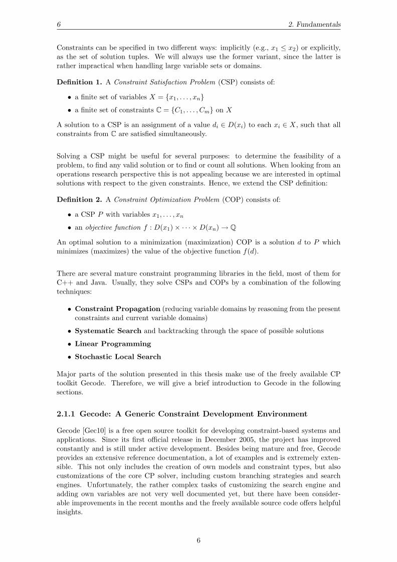
Constraints can be specified in two different ways: implicitly (e.g., x1 ≤ x2) or explicitly,as the set of solution tuples. We will always use the former variant, since the latter israther impractical when handling large variable sets or domains.

Definition 1. A Constraint Satisfaction Problem (CSP) consists of:

• a finite set of variables X = {x1, . . . , xn}

• a finite set of constraints C = {C1, . . . , Cm} on X

A solution to a CSP is an assignment of a value di ∈ D(xi) to each xi ∈ X, such that allconstraints from C are satisfied simultaneously.

Solving a CSP might be useful for several purposes: to determine the feasibility of aproblem, to find any valid solution or to find or count all solutions. When looking from anoperations research perspective this is not appealing because we are interested in optimalsolutions with respect to the given constraints. Hence, we extend the CSP definition:

Definition 2. A Constraint Optimization Problem (COP) consists of:

• a CSP P with variables x1, . . . , xn

• an objective function f : D(x1)× · · · ×D(xn)→ Q

An optimal solution to a minimization (maximization) COP is a solution d to P whichminimizes (maximizes) the value of the objective function f(d).

There are several mature constraint programming libraries in the field, most of them forC++ and Java. Usually, they solve CSPs and COPs by a combination of the followingtechniques:

• Constraint Propagation (reducing variable domains by reasoning from the presentconstraints and current variable domains)

• Systematic Search and backtracking through the space of possible solutions

• Linear Programming

• Stochastic Local Search

Major parts of the solution presented in this thesis make use of the freely available CPtoolkit Gecode. Therefore, we will give a brief introduction to Gecode in the followingsections.

2.1.1 Gecode: A Generic Constraint Development Environment

Gecode [Gec10] is a free open source toolkit for developing constraint-based systems andapplications. Since its first official release in December 2005, the project has improvedconstantly and is still under active development. Besides being mature and free, Gecodeprovides an extensive reference documentation, a lot of examples and is extremely exten-sible. This not only includes the creation of own models and constraint types, but alsocustomizations of the core CP solver, including custom branching strategies and searchengines. Unfortunately, the rather complex tasks of customizing the search engine andadding own variables are not very well documented yet, but there have been consider-able improvements in the recent months and the freely available source code offers helpfulinsights.

6

2.1. Constraint Programming 7

Basics

The central object in a Gecode model is a so-called space. It describes the current state ofour world/model, including all variables, their respective domains and all the constraintsa solution has to fulfill. Adding further constraints to a space is called posting.

In the remainder of this section we give a short introduction to the different componentsof a Gecode model. For further reading we recommend the great introduction ”Modellingand Programming with Gecode” [STL10] and the dissertation about ”Constraint Propaga-tion” [Tac09] by one of the main contributors of Gecode.

2.1.2 Models and Constraints

One of the models offered by Gecode to formulate constraint programs are finite domainintegers (FDI). An FDI variable can take any integer of its domain – a finite set of 32-bitintegers. Note that we can also model logical values using an FDI variable with a domainof {0; 1}.

The general procedure performed by the CP solver is as follows. In the beginning a spaceis set up and all its variables are only limited by their initial domain (e.g., D(x1) ={1, . . . , 10}, D(x2) = {4, . . . , 10}). First, a phase of constraint propagation is performed,to limit these domains by reasoning from the given constraints (e.g., x1 > x2 ⇒ D(x1) ={5, . . . , 10}∧D(x2) = {4, . . . , 9}). We call a state where no further propagation is possiblein the space a fix point. A branching now splits the search space into (generally) twobranches. One branch usually gets one variable assigned to a value of its domain, while thisvalue is excluded from the variables domain in the second branch. After that, constraintpropagation can be applied to both branches and the process repeats until there are nomore unassigned variables, i.e., a valid solution is found. Usually, this search process isorganized as a depth first search in the search tree formed by the branching.

The details of propagation, branching and search will be explained in the following sections.Let us first have a look on the constraint types for finite domain integers provided byGecode, which will be relevant for our upcoming problem formulation:

Domain constraints: The domain of a variable is specified by a lower and upper boundor is defined as a set of integers.

Relational constraints: These constraints can be used to enforce different types of binaryrelations (e.g., >,≥,=, 6=,≤, <) between different variables or between a variable anda constant. They can also be used in another way, where the relation is not enforced,but is evaluated and assigned to a boolean-valued FDI variable (e.g., x < y ⇔ b).Most relational constraints can be naturally applied to arrays of variables.

Linear constraints: They can be used to determine a (weighted) sum of an array of vari-ables and model a relation between the result and another variable or constant (e.g.,∑

i ai · xi ≤ y). Similar to the relational constraints, there is an option to evaluatethe relation and assign its result (true or false) to another variable.

Arithmetic constraints: A variety of basic arithmetic operations can by applied to vari-ables and constants. This includes basic binary operators (+, −, ∗, /, mod) as wellas unary ones (square and square root, absolute value) and operations on arrays ofvariables (minimum, maximum). The result of this operation is always related toanother variable by equality (e.q. x1 ∼ x2 = x3).

Scheduling constraints: This is one of the more sophisticated constraint types of Gecode.They model resource limits when scheduling a set of unsplittable jobs onto a set ofmachines. Jobs are given by their possible start/end dates, duration and resource

7

8 2. Fundamentals

consumption. The machines are given by their respective resource amount per unit oftime. Resource limits can be either upper or lower bounds. Note that this constraintdoes not actively schedule the dates, but limits each jobs start/end domain to feasiblevalues, considering the available machines and states of the other jobs. See [BC02]for details.

Relational constraints on boolean variables (like ∨, ∧, ⇒, ⇔) can also be modelled usingarithmetic and relational constraints (e.g., A ⇒ B is equivalent to B − A ≥ 0). Addi-tionally, Gecode provides a variety of other constraint types like array element, distinct,channel, sorted, cardinality and graph constraints which we will not introduce here, sincethey do not appear in our model.

To ease the effort required for modeling, there is a so-called direct modeling supportprovided by Gecode (technically it is overloading C++ operators). These functions allowus to formulate constraints in a very natural way. For example the constraint (x + y <23)⇒ z = 42 would look like:

post(space, tt(imp( ~(x + y < 23), ~(z == 42))))

2.1.3 Propagation

In Gecode constraints are implemented as so-called propagators. When set up, each propa-gator subscribes to its affected variables. Later, it is notified on changes of these variables’domains. When called because of changes to a variable x, the propagator checks if thesmaller domain of x helps to reduce the domains of other variables. We call this processpropagation and the reduction of domains filtering. Filtering does not change the set ofsolutions. Furthermore, a propagator manipulating the domain of a variable possibly trig-gers further propagator execution (including of itself). This notification/execution schemeis repeated until we either reach a fix point or a domain becomes empty. We call the lattera failed space.

We can distinguish between different strengths of filtering. A filtering for a constraint Cis complete if each removal of a value from the residual variable domains would reduce theset of solutions for C. Otherwise, all filterings where additional narrowing of a domainwould be possible are called partial. We will now formalize two so-called consistency levels,which arise from the filtering strengths (cf. [RBW06]):

Definition 3. (Domain Consistency) Let C be a constraint on the variables x1, . . . , xnwith their respective domains D(xi) for every 1 ≤ i ≤ n. We say that C is domainconsistent if for 1 ≤ i ≤ n and v ∈ D(xi), there exists a tuple (d1, . . . , dn) ∈ C such thatdi = v. A CSP is domain consistent if each of its constraints is domain consistent.

Definition 4. (Bound Consistency) Let C be a constraint on the variables x1, . . . , xnwith respective lower and upper bounds L(x1), U(x1), . . . , L(xn), U(xn). We say that C isbound consistent if both (L(x1), . . . , L(xn)) ∈ C and (U(x1), . . . , U(xn)) ∈ C.

We illustrate both consistency types in a short example. Let us assume that we have twovariables with domains D(x1) = {1, . . . , 5}, D(x2) = {1, . . . , 6, 8} and a single constraintx1 +x2 = 10. A close look reveals that the domain consistent fix point is D(x1) = {2, 4, 5}and D(x2) = {5, 6, 8}. Note that it is generally hard (even NP-hard) to find such a fixpoint. Using the variables’ bounds (L(x1) = 1, U(x1) = 5, L(x2) = 1, U(x2) = 8) we canderive that x1 ≥ 2 and x2 ≥ 5, thus resulting in a slightly weaker bound consistent fixpoint at D(x1) = {2, . . . , 5} and D(x2) = {5, 6, 8}.

8

2.1. Constraint Programming 9

Gecode offers three different notification levels for propagators, derived from these con-sistency levels. In the strongest, domain level, a propagator gets notified of all domainchanges of its subscriptions. In bound level, the system notifies a propagator if either thelower or upper bound of a subscribed variable is modified. Finally, the weakest level, valuelevel, only notifies propagators if a subscribed variable gets assigned, i.e., when its domainsize becomes exactly one.

Execution costs between these levels may vary greatly. Although domain consistency yieldsthe strongest filtering, it might be computationally hard to achieve. The weaker levels canprovide a significant speedup at the cost of a reasonably poorer filtering. Thus, one cantweak a model by choosing the right notification levels for the propagators.

2.1.4 Branching

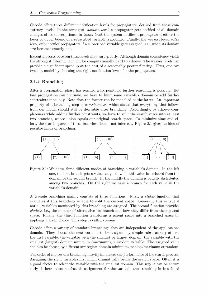
After a propagation phase has reached a fix point, no further reasoning is possible. Be-fore propagation can continue, we have to limit some variable’s domain or add furtherconstraints manually. Note that the former can be modelled as the latter. An importantproperty of a branching step is completeness, which states that everything that followsfrom our model should still be derivable after branching. Accordingly, to achieve com-pleteness while adding further constraints, we have to split the search space into at leasttwo branches, whose union equals our original search space. To minimize time and ef-fort, the search spaces of these branches should not intersect. Figure 2.1 gives an idea ofpossible kinds of branching.

{1, . . . , 10}

{1} {2, . . . , 10}

{1, . . . , 10}

{1, . . . , 5} {6, . . . , 10}

{1, . . . , 10}

{1} {10}. . .

Figure 2.1: We show three different modes of branching a variable’s domain. In the leftone, the first branch gets a value assigned, while this value is excluded from thedomain of the second branch. In the middle the domain is equally distributedamong two branches. On the right we have a branch for each value in thevariable’s domain.

A Gecode branching mainly consists of three functions. First, a status function thatevaluates if this branching is able to split the current space. Generally this is true ifnot all variables monitored by this branching are assigned. The second function provideschoices, i.e., the number of alternatives to branch and how they differ from their parentspace. Finally, the third function transforms a parent space into a branched space byapplying a given choice. This step is called commit.

Gecode offers a variety of standard branchings that are independent of the applicationsdomain. They choose the next variable to be assigned by simple rules, among others:the first variable, the variable with the smallest or largest domain, the variable with thesmallest (largest) domain minimum (maximum), a random variable. The assigned valuecan also be chosen by different strategies: domain minimum/median/maximum or random.

The order of choices of a branching heavily influences the performance of the search process.Assigning the right variables first might dramatically prune the search space. Often it isa good choice to select the variable with the smallest domain. This way it can be shownearly if there exists no feasible assignment for the variable, thus resulting in less failed

9

10 2. Fundamentals

spaces throughout the remaining search process. Accordingly, we can say that the numberof failed spaces visited during the search attributes to the quality of a branching.

For most problems there exist good heuristics to decide which variable to assign next andwhich value to choose. Gecode offers a way to implement such heuristics in custom branch-ings and to use them in the search process. This way, one might get better performanceand branching quality (i.e., less failed spaces).

2.1.5 Search Engines

Gecode offers several search engines which roughly control the search process. Basically,the engine decides about the order of traversal of the search tree formed by the branchingsand their respective choices. A common search engine for solving constraint models is asimple depth-first search. At each node of the search tree, the engine commits the firstalternative of the choice of one of the present branchings. After each commit a propagationphase takes place. If the domain of at least one variable becomes empty, i.e., a failed spaceis reached, a backtrack step is performed and the next alternative is chosen. This isrepeated until no branching can split the search space anymore – a solution is found – orthe whole search tree has been traversed.

One notable problem of a depth-first search on large search spaces is that bad assignmentsof the first branched variables can hardly be revised. In this case, the whole – possiblyhuge – subtree has to be evaluated before a decision can be revoked. We will overcomethis problem by restarting the search process after a certain number of failed spaces hasbeen reached and by randomizing choices.

2.2 Graphs and Networks

In this section we briefly introduce the main graph theoretic concepts that will appearin the upcoming chapters. For a general introduction to the topic we refer to [CLRS01].Detailed information about network flows can be found in [AMO93].

Definition 5. (Digraph) A directed graph is a pair G = (V,E), where V is a finite setof vertices and E ⊆ V × V is a set of ordered pairs of vertices, called arcs. An arc fromu ∈ V to v ∈ V is denoted by (u, v).

Definition 6. (Flow Network) A flow network N = (G, cap, s, t) consists of a directedgraph G = (V,E), a capacity function cap : E → [R≥0,R≥0] and two distinguished vertices:a source s and a target t. For each arc the capacity function returns a non-empty interval.If (u, v) /∈ E, we assume cap(u, v) := [0, 0].

Definition 7. (Flow) Let N = (G, cap, s, t) be a flow network. A valid flow is a functionf : V × V → R, which satisfies the following three properties:

• Capacity constraint: ∀u, v ∈ V : f(u, v) ∈ cap(u, v)

• Skew symmetry: ∀u, v ∈ V : f(u, v) = −f(v, u)

• Flow conservation: ∀u ∈ V \ {s, t} :∑v∈V

f(u, v) = 0

Definitions 6 and 7 differ slightly from the definitions found in the mentioned textbooks,because we introduce the additional feature of a lower bound of the capacity function.But, such a network can be transformed into a network without a lower capacity bound(see Figure 2.2), but where any valid flow has to saturate certain arcs.

10

2.2. Graphs and Networks 11

s tu v[l, h]

s tu v

l

h− l

l

Figure 2.2: Removal of minimum capacities: The arc (u, v) in the upper network has aminimum capacity of l. The lower network does not comprise minimum ca-pacities anymore, but each valid flow has to saturate the new arcs incident tos and t.

Definition 8. (Minimum Cost Flow Problem) Let N = (G, cap, s, t) be a flow network,cost : V × V → R a cost function of each arc and d the required amount of flow. Theminimum-cost flow problem P = (N, cost) is to find a valid flow f that minimizes the costfunction when implementing a flow of size d in the network:

• Required Flow: d =∑u∈V

f(s, u) =∑u∈V

f(u, t)

• Objective Function: minf

∑(u,v)∈E

f(u, v) · cost(u, v)

There are several algorithms available to solve the minimum cost flow problem. For ourexperiments we use an implementation of the cost scaling algorithm [GT90] which is partof the Lemon Graph Library [Lem10]. The algorithm runs in O(n3 log(nC)) where C isthe maximum absolute integer-valued arc cost.

While modeling a part of our problem as a flow network, we identify costs that do notdepend on the implemented flow in the network. We will extract these costs into a globalcost offset and adjust the value of the objective function accordingly:

cost(f) := global cost offset +∑

(u,v)∈E

f(u, v) · cost(u, v)

11

12 2. Fundamentals

12

3. Problem Statement

This chapter introduces the problem proposed by the ROADEF/EURO Challenge 2010in [PGJ+] and sets up the model used throughout this thesis. The problem definition wasmainly developed by the French utility company EDF and therefore also contains somefeatures of French energy policy. Furthermore, all problem instances are provided by EDF.

We begin with an introduction to the topic in Section 3.1 to the model, followed by somegeneral definitions in Section 3.2. Besides some domain-specific terminology, this sectionintroduces the indices, variables and auxiliary constructs used in the model. Afterwards,Section 3.3 presents the core of the model: various constraint types separated into pro-duction related constraints (i.e., technical constraints of each single power plant) andoutage scheduling constraints (i.e., constraints between different power plants). Finally,Section 3.4 shows a formal definition of the objective function.

Parts of this chapter replicate the ROADEF/EURO Challenge 2010 subject document.We slightly modify the model proposed there to remove redundancies and to make param-eters, function signatures and indexing consistent and easier to understand. There are noconceptual changes.

3.1 Introduction

In the following we introduce a model for medium-term electricity production planningutilizing a large set of power plants. As it is a tactical model, we neither make any strategicdecisions (like adding/removing power plants) nor do we care for short-term operationalrestrictions (like intraday load following). Although the model comprises some peculiaritiesof the French energy market (see [Kid09]), it should be useful in different contexts.

The model extends over a period of time (e.g., 5 years). This period is split into uniformtime steps of configurable length (e.g., 1 day). The two first class entities of our model area set of various power plants and a set of uncertainty demand scenarios (see Figure 3.1).For each scenario we are looking for a production assignment, such that the sum of energyproduced by all available power plants equals the demand during each time step. The needfor multiple scenarios arises from the numerous uncertainties that have to be taken intoaccount (e.g., unknown energy demand, generation units availability, spot market prices,quantities that can be bought or sold, . . .).

In our model there are two very different types of facilities. Power plants of the first typecan operate continuously and their fuel supply is outside the scope of our problem. During

13

14 3. Problem Statement

Power Plants Demand Scenarios

?

Figure 3.1: On the left, we have an inhomogeneous set of power plants, on the right, a setof demand scenarios. For each scenario we have to generate a production plandistributing the demand among the power plants.

1

Scenario 0

prod

ucti

on

min

max

real· · ·

unit

cost

· · ·

Scenario s

· · ·

· · ·

Figure 3.2: Sample plots illustrating the development of production and unit cost overtime of a Type-1 power plant for different scenarios. In the upper plots thered (blue) lines show the minimum (maximum) allowed production. The greenlines are production plans. In the lower plots the red lines show the cost perunit of energy produced by this plant.

each time step they can produce an amount of energy in an interval depending on thescenario and time step (see Figure 3.2). We call them Type-1 power plants. Production atthese power plants induces cost that is proportional to the power output of a plant andalso depend on the scenario and time step. Power plants of this type might be coal- orgas-fired or even virtual power plants for exporting and importing energy, whose availablepower levels and unit cost we cannot influence.

The other type of power plants, called Type-2 power plants, has to be shut down forrefueling and maintenance regularly. Therefore, modeling these facilities requires moreeffort. As the plants have only limited capacities to store fuel and running out of itwould stop the production of energy, these power plants have to be refueled regularly (seeFigure 3.3). Refueling can only take place when a power plant is offline for several weeks.Hence, the operation of a Type-2 power plant is organized in cycles – successions of anoffline period (an outage with refueling and maintenance) and the following productioncampaign. It might not be necessary to schedule all cycles of a Type-2 power plant beforethe end of the time horizon, i.e., we can postpone outages. But the order of a power plant’scycles is fixed and so all successive cycles would have to be postponed, too.

Contrary to Type-1 power plants, production at Type-2 power plants is billed via theamount of fuel reloaded. In the model, the fuel unit cost depends on the cycle and power

14

3.2. General Definitions 15

2

Scenario 0

prod

ucti

on max

real

Outage

· · ·

fuel

leve

l Refueling· · ·

Scenario s

· · ·

· · ·

Figure 3.3: Sample plots illustrating the production and fuel levels over time of a Type-2power plant for different scenarios. In the upper plots the gray areas show theallowed production interval. The green line is a production plan. Note thatthe outage dates (red area) and refueling amounts (upturns of the cyan line)are equal in all scenarios.

plant. For each Type-2 power plant a number of (fuel-related) production constraintsapply. Furthermore, outages of different Type-2 power plants are dependent on each otherto fulfill resource, staff, grid stability, production safety and legal restrictions. Power plantsof this type are generally nuclear power plants.

To conclude, the proposed subject consists of modeling the production assets and findingan optimal outage schedule. It includes two dependent subproblems:

1. Determine a schedule of plant outages. This schedule must satisfy the given con-straints in order to comply with limitations on resources, which are necessary toperform refueling and maintenance operations.

2. Determine an optimal production plan to satisfy demand, i.e., a quantity of energyto produce by each plant at each time step for each scenario.

The objective is to minimize the expected cost of production.

3.2 General Definitions

In this section, we define domain-specific terminology, indices, decision variables and prob-lem parameters, which will be used by the constraint definitions in the next section andall following parts of this thesis.

3.2.1 Terminology

First, we introduce some words with domain-specific meaning:

Time Step: The time horizon is split into discrete periods of time of the same length. Atime step is the smallest unit of time we deal with, i.e., our world is constant duringa time step.

Week: A (per dataset) fixed number of successive time steps. Note that power plantoutages are scheduled in weeks, while production levels will be planned for each timestep.

Scenario: The demand to be satisfied by all plants is given in the form of different uncer-tainty scenarios. Each scenario is given as a vector of concrete production amounts(i.e., one value per time step), which can be seen as the result of some stochasticprocess.

15


The following terms apply only to Type-2 power plants:

Outage: A series of weeks during which a plant is offline.

Production Campaign: A series of weeks during which a plant can produce.

Cycle: The succession of an outage and a production campaign.

Decoupling: The first week of an outage.

Coupling: The first week of a production campaign.

Reloading/Refueling: The amount of fuel provided during an outage.

Modulation: The sum of the differences between the maximum allowed and actual pro-duction over all time steps of a production campaign.

Imposed Power Profile: A constraint imposing that the production level of a plant hasto follow a given profile if the fuel level is below a certain threshold.

3.2.2 Indices

A dataset comprises various sets of entities. Let S denote the set of the scenarios, J theset of Type-1 power plants and I the set of Type-2 power plants. Our timeline consistsof T uniform time steps spanning over W weeks in total, where T is always a multiple ofW. We define the corresponding sets for time steps as T = {0, . . . ,T−1} and weeks asW = {0, . . . ,W−1}.

We denote the number of cycles of each Type-2 power plant as K and the correspondingset as K = {0, . . . ,K−1}. K is equal for all Type-2 power plants. Furthermore, we denotethe cycle and production campaign each plant starts with (i.e., during time step 0) asthe initial cycle and use k = −1 for it. Similarly, we use K, T and W in the upcomingparameters to denote the end of our time horizon.

The following lower case indices will be used throughout this document to access singleentities of the given type: s ∈ S, j ∈ J , i ∈ I, t ∈ T , w ∈ W, k ∈ K.

3.2.3 Decision Variables

The following three types of decision variables make up our problem:

Decoupling Dates: Each Type-2 power plant regularly goes offline for refueling and main-tenance. Let hai,k ∈ {−1} ∪ W denote the week of decoupling of plant i in cyclek. Note that there are two special cases. First, for the initial cycle of each plantwe define hai,−1 := 0. Second, if a cycle is not scheduled, i.e., its decoupling date ispostponed behind the time horizon, then hai,k will be set to −1.

Refueling Amounts: During each outage a Type-2 power plant can be supplied with acertain of amount of fuel. Let ri,k ∈ R≥0 denote this amount of plant i in cycle k.We define the refueling amount of postponed cycle as 0.

Production Levels: In a solution all power plants (i.e., both types) need to have an ab-solute real-valued production level assigned for each time step and scenario. Letpj,s,t/pi,s,t ∈ R≥0 denote this level of power plant j/i during time step t in scenario s.

Note that a power plant’s production levels may vary between demand scenarios of adataset, while outage dates and refueling amounts are decision variables of the dataset,i.e, they are equal in all scenarios.

3.2.4 Global Parameters

• DEMs,t: Demand to satisfy for scenario s and time step t

• D: Length of a time step (all time steps have equal length)

16

3.2. General Definitions 17

3.2.5 Parameters of each Type-1 Power Plant j

• PMINs,tj : Minimum production level during time step t of scenario s

• PMAXs,tj : Maximum production level during time step t of scenario s

• Cs,tj : Cost of production per unit during time step t of scenario s

3.2.6 Parameters of each Type-2 Power Plant i

• PMAXti: Maximum production level during time step t in all scenarios

• XIi: Initial fuel level (i.e., in time step 0)

• Ci,T: Discount per unit for residual fuel at the end of the time horizon

The following parameters are provided for each cycle k of a Type-2 power plant:

• DAi,k: Duration of the outage in weeks (note the special case DAi,−1 := 0)

• Ci,k: Cost of refueling per unit during this cycle’s outage

• RMINi,k: Minimum refueling amount

• RMAXi,k: Maximum refueling amount

• MMAXi,k: Maximum modulation over production campaign

• Qi,k: Refueling coefficient (see constraint 10)

• BOi,k: Fuel level threshold activating the imposed power profile for this campaign

• PBi,k: Decreasing power profile (a piece–wise linear concave function: R≥0 → [0, 1])

• ε: Tolerance for the imposed power profile

• AMAXi,k: Upper bound of fuel level before refueling

• SMAXi,k: Upper bound of fuel level after refueling

Additionally, the parameters MMAXi,−1, BOi,−1 and PBi,−1 will also be provided.

3.2.7 Auxiliary Constructs

We define some auxiliary constructs for Type-2 power plants, which will come in handyfor the upcoming constraint definitions:

Definition 9. Given an arbitrary Type-2 power plant i and a production cycle k, lett−i,k denote the first time step of this cycle (which is also the first time step of the outage),t∗i,k denote the first time step of this cycle’s production campaign and t+i,k denote the firsttime step after the end of this cycle. For a not scheduled cycle all three variables equal T.Formally we define:

hai,k 6= −1 =⇒ t−i,k = hai,k · T /W

hai,k 6= −1 =⇒ t∗i,k = (hai,k + DAi,k) · T /W

hai,k+1 6= −1 =⇒ t+i,k = hai,k+1 · T /W

Note that t+i,k generally corresponds to t−i,k+1 with exceptions for the initial cycle, wheret−i,−1 = t∗i,−1 = 0, and the last cycle, where t+i,K−1 = T.

Definition 10. Let x(i, s, t) denote the fuel level of plant i at the beginning of time stept in scenario s. For each plant and scenario the fuel level of a time step depends on the fuellevel of the previous time step and the production level and refueling performed duringthe previous time step. See the constraints 9 and 10 for the details. Note that x(i, s,T)denotes the fuel level at the end of the time horizon.

17


3.3 Constraints

In this section we define the constraints that make up our model. We adopt the numberingfrom the official problem statement of the competition. In the first part we model plantoperations (production levels, fuel level variation, fuel level restrictions). The second partpresents different types of outage constraints between Type-2 power plants which arise fromlimited resources (staff, tools, . . .), legal restrictions and production safety considerations.

[CT 1] Coupling load and production

The sum of production of all Type-1 power plants and all Type-2 power plants equals thedemand DEMs,t in all scenarios s and time steps t:∑

j∈Jpj,s,t +

∑i∈I

pi,s,t = DEMs,t s ∈ S; t ∈ T

3.3.1 Production Related Constraints

[CT 2] Bound of production of Type-1 power plants

The production pj,s,t of a Type-1 power plant j has to stay between its lower boundPMINs,t

j and upper bound PMAXs,tj . These bounds may also model outages which are

outside the scope of our problem:

PMINs,tj ≤ pj,s,t ≤ PMAXs,t

j j ∈ J ; s ∈ S; t ∈ T

[CT 3] Offline power

During every time step t where a Type-2 power plant i is on outage, its production pi,s,tequals zero in all scenarios s:

pi,s,t = 0 i ∈ I; s ∈ S; t ∈⋃k∈K

[t−i,k, t∗i,k − 1]

[CT 4] Bound of production of Type-2 power plants

During every time step t the production pi,s,t of a Type-2 power plant i is between zeroand the upper bound PMAXt

i:

0 ≤ pi,s,t ≤ PMAXti i ∈ I; s ∈ S; t ∈ T

[CT 5] Maximum power before power profile imposition

We merged this constraint with CT 4.

[CT 6] Maximum power after power profile imposition

If the fuel level x(i, s, t) of a Type-2 power plant i drops below the cycle’s threshold BOi,k,then the production pi,s,t is fixed to the given ratio PBi,k : R≥0 → [0, 1] of PMAXt

i withina tolerance of ε, as long as there is enough fuel x(i, s, t) to cover the current consumption:

PBi,k(x(i, s, t)) · PMAXti ·D ≤ x(i, s, t) < BOi,k =⇒

(1− ε)(PBi,k(x(i, s, t)) · PMAXti) ≤ pi,s,t ≤ (1 + ε)(PBi,k(x(i, s, t)) · PMAXt

i)

If there is not enough fuel left to fulfill the imposed production amount, then this powerplant cannot produce anything:(

x(i, s, t) < BOi,k

)∧(x(i, s, t) < PBi,k(x(i, s, t)) · PMAXt

i ·D)

=⇒ pi,s,t = 0

18

3.3. Constraints 19

[CT 7] Bounds of refueling

If a cycle k of Type-2 power plant i is scheduled (i.e., hai,k 6= −1), then the performedrefueling ri,k is between its lower bound RMINi,k and upper bound RMAXi,k:

hai,k 6= −1 =⇒ RMINi,k ≤ ri,k ≤ RMAXi,k i ∈ I; k ∈ K

[CT 8] Initial fuel level

For each Type-2 power plant i, the fuel level x(i, s, t) of the first time step equals theplant’s initial fuel level parameter XIi:

x(i, s, 0) = XIi i ∈ I; s ∈ S

[CT 9] Fuel level variation during a production campaign

Fuel levels are passed between successive time steps and adjusted by the fuel consumption,which is calculated from the production level pi,s,t and the time steps duration D:

x(i, s, t+ 1) = x(i, s, t)− pi,s,t ·D i ∈ I; s ∈ S; t ∈⋃k∈K

[t∗i,k, t+i,k − 1]

Note that fuel levels cannot be negative:

x(i, s, t) ≥ 0 i ∈ I; s ∈ S; t ∈ T ∪ {T}

[CT 10] Fuel level variation during an outage

In the process of refueling a Type-2 power plant i, a certain amount of unspent fuel has tobe removed to make the addition of new fuel possible. The refueling coefficient Qi,k helpsto quantify this amount. Note that the fuel threshold BOi,k is in reality part of the reload– refueling ri,k and threshold BOi,k have been separated in the formulation because one isa decision variable and the other is imposed (a technical parameter).

Refueling is performed entirely during the first timestep t−i,k of an outage:

x(i, s, t−i,k + 1) =Qi,k−1

Qi,k

(x(i, s, t−i,k)− BOi,k−1) + ri,k + BOi,k i ∈ I; s ∈ S; k ∈ K

There is no further fuel variation during an outage.

[CT 11] Fuel level bounds around refueling

The fuel levels before and after refueling of a Type-2 power plant i and cycle k are restrictedby AMAXi,k and SMAXi,k respectively:

0 ≤ x(i, s, t−i,k) ≤ AMAXi,k

x(i, s, t−i,k + 1) ≤ SMAXi,k

i ∈ I; s ∈ S; k ∈ K

[CT 12] Maximum modulation over a cycle

While production is not imposed (see CT 6), the production campaign’s aggregated devi-ation from the maximum production PMAXt

i is limited by MMAXi,k. If the fuel level isbelow BOi,k then the imposed power profile determines the exact production level.∑

t∗i,k≤t<t+i,k

x(i,s,t)≥BOi,k

(PMAXt

i−pi,s,t)·D ≤ MMAXi,k i ∈ I; s ∈ S; k ∈ K

19


3.3.2 Outage Scheduling Constraints

The following constraints set up relations between outages of different Type-2 power plants.A dataset might contain multiple instances of the constraint types 14 to 21 for varyingsubsets of plants and with different parameters. Note that all these constraint instancesare independent and do not share any parameters.

[CT 13A] Earliest and latest date of outage

An outage has to start during a given interval or may not be scheduled.

Data:

• i: The given Type-2 power plant

• k: The given outage/cycle

• TOi,k: First possible week of decoupling

• TAi,k: Latest week of decoupling (or −1 if the cycle can be postponed)

Constraint:

TAi,k 6= −1 =⇒ TOi,k ≤ hai,k ≤ TAi,k

TAi,k = −1 =⇒ hai,k = −1 ∨ TOi,k ≤ hai,k

[CT 13B] Order of outage

Outages of a Type-2 power plant i appear in the same order as presented in the datasetand do not overlap (remember DAi,k as outage duration). Therefore, if we decide not toschedule an outage, all successive outages of the same plant have to be postponed, too.

Constraint:

hai,k 6= −1 =⇒ hai,k−1 + DAi,k−1 ≤ hai,khai,k−1 = −1 =⇒ hai,k = −1

i ∈ I; k ∈ K

3.3.3 Outage Dependency Constraints

The following constraints operate on a subset of Type-2 power plants A ⊆ I and only ontheir scheduled cycles.

Data:

• A: Set of considered Type-2 power plants

3.3.3.1 Spacing Constraints

The following constraints define minimum spacings (or maximum overlappings, respec-tively) between scheduled cycles from power plants of the set A.

Data:

• Se: Duration in weeks of minimum authorized spacing. Negative values are inter-preted as maximum authorized overlapping.

20

3.3. Constraints 21

[CT 14] Minimum spacing/Maximum overlapping between outages

This constraint defines a set of Type-2 power plants A whose outages have to be scheduledwith a minimum pairwise spacing (or maximum overlapping) of Se weeks.

Constraint:

(hai,k − hai′,k′ −DAi′,k′ ≥ Se

)∨

(hai′,k′ − hai,k −DAi,k ≥ Se)i, i′ ∈ A; k, k′ ∈ K; i 6= i′

[CT 15] Minimum spacing/Maximum overlapping between outages during aspecific period

Outages of a set A of Type-2 power plants that intersect an interval [ID, IF] have to bescheduled with a minimum pairwise spacing (or maximum overlapping) of Se weeks.

Data:

• ID: First week of the specific period

• IF: Last week of the specific period

Constraint:

(ID−DAi,k +1 ≤ hai,k ≤ IF

)∧(

ID−DAi′,k′ +1 ≤ hai′,k′ ≤ IF)

=⇒(hai,k − hai′,k′ −DAi′,k′ ≥ Se

)∨(

hai′,k′ − hai,k −DAi,k ≥ Se) i, i′ ∈ A; k, k′ ∈ K; i 6= i′

[CT 16] Minimum spacing between decoupling dates

Decoupling dates of outages from a set A of Type-2 power plants have to be spaced by atleast Se weeks.

Constraint:

|hai,k − hai′,k′ | ≥ Se i, i′ ∈ A; k, k′ ∈ K; i 6= i′

[CT 17] Minimum spacing between coupling dates

Coupling dates of outages of a set A of Type-2 power plants have to be spaced by at leastSe weeks.

Constraint:

|hai,k + DAi,k−hai′,k′ −DAi′,k′ | ≥ Se i, i′ ∈ A; k, k′ ∈ K; i 6= i′

[CT 18] Minimum spacing between decoupling and coupling dates

Decoupling dates and coupling dates of outages of a set A of Type-2 power plants have tobe spaced by at least Se weeks.

21


Constraint:

|hai,k + DAi,k−hai′,k′ | ≥ Se i, i′ ∈ A; k, k′ ∈ K; i 6= i′

3.3.3.2 Resource Constraints

The following constraints aggregate values if a condition holds. Therefore, we first definean indicator function:

1([l, h), x

)={

1 if x ∈ [l, h)0 else

[CT 19] Limited resources

Each outage of a set A of Type-2 power plants requires one unit of the given resourceduring certain weeks of its outage. All outages have to be scheduled with respect to thelimited availability of the resource, i.e., there is no week w where the resource limit isexceeded.

Data:

• Li,k: First week of resource usage (0 ≤ Li,k < DAi,k)

• TUi,k: Time of usage of the resource in weeks (0 ≤ TUi,k; Li,k + TUi,k ≤ DAi,k)

• Q: Available quantity of the resource

Constraint:

∑i∈Ak∈K

hai,k 6=−1

1([hai,k + Li,k, hai,k + Li,k + TUi,k), w

)≤ Q w ∈ W

[CT 20] Maximum number of outages during a given week

The number of outages among a set A of Type-2 power plants during a specific week canbe limited.

Data:

• H: The considered week

• N: Maximum number of outages during this week

Constraint:

∑i∈Ak∈K

hai,k 6=−1

1([hai,k, hai,k + DAi,k),H

)≤ N

[CT 21] Maximum offline power capacity during a specific period

During the given period the aggregated maximum production capacity of all plants onoutage from a set A can be limited.

22

3.4. Objective Function 23

Data:

• ID: First time step of period

• IF: Last time step of period

• IMAX: Maximum offline power capacity

Constraint:

∑i∈AS

k∈K[t−i,k,t∗i,k−1]3t

PMAXti ≤ IMAX t ∈ T ; ID ≤ t ≤ IF

3.4 Objective Function

While satisfying all given constraints (CT 1 – 21) the sum of the following two terms is tobe minimized:

• The expected production cost of all Type-1 power plants over all scenarios.

• The total refueling cost of all Type-2 power plants reduced by the expected value ofresidual fuel at the end of the time horizon over all scenarios.

We can formalize our objective function as follows:

∑i∈I

∑k∈K

Ci,k ·ri,k︸︷︷︸PP2 refueling cost

+1|S|∑s∈S

(∑t∈T

(∑j∈J

Cs,tj ·pj,s,t ·D︸︷︷︸

PP1 production cost

)−∑i∈I

Ci,T ·x(i, s,T)︸︷︷︸PP2 residual fuel refund

)

Note that the refueling amounts and refueling unit costs are constant in all scenarios.Contrary, the unit production costs of Type-1 power plants and residual fuel amounts ofType-2 power plants can vary between scenarios and have to be averaged.

23


24

4. Lower Bounds

In this chapter we present two lower bounds for the overall solution cost of a given dataset,which have several useful applications. For example, they can be used to evaluate thequality of found solutions and – since our considered search spaces are far too big to befully explored – to decide when to stop the search. Furthermore, a lower bound that is fastto compute can be used to guide the search into promising regions of the solution space.

Before composing the first bound for our main problem, we develop a lower bound forType-2 power plant unit production costs, which is presented in Section 4.1. Then, wepresent the first lower bound for the entire problem – utilizing a cheapest-first auction– in Section 4.2. This bound provides a vantage point for a simple and correct greedyproduction assignment heuristic presented later.

A more sophisticated lower bound, which also considers most of the fuel level and refuelingconstraints, is presented in Section 4.3. It employs a flow network to model productionlevels and refueling amounts.

4.1 Type-2 Power Plant Unit Production Cost

In contrast to Type-1 power plants, the production of Type-2 power plants is not chargedvia the produced amounts of energy but with the fuel reloaded during each outage. Inthis section, we set up a simple lower bound for the unit production cost (UPC) of eachType-2 power plant in a given dataset. This lower bound will enable us to compare theUPC of all plants and – in a next step – assign production to the cheapest plants.

There are several hurdles to overcome while transforming reloading costs into productioncosts:

• The initial fuel level is provided for free.

• Refueling unit costs vary with each cycle (CT 7).

• Refueling is not just adding fuel – we can lose or gain fuel for free (CT 10).

• There is a refund for residual fuel at the end of the time horizon.

For this bound we will assume that Type-2 power plants can produce in each time step, i.e.,there are no scheduled outage periods. Furthermore, we relax the following constraints:

CT 6 : Maximum power after power profile imposition

25

26 4. Lower Bounds

CT 7 - 11 : Fuel level tracking constraints

CT 12 : Maximum modulation over a cycle

CT 13 - 21 : Outage dependency constraints

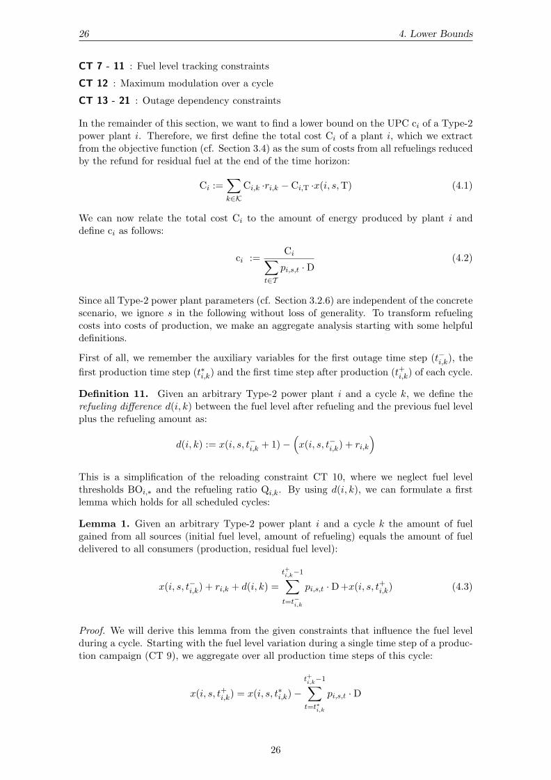
In the remainder of this section, we want to find a lower bound on the UPC ci of a Type-2power plant i. Therefore, we first define the total cost Ci of a plant i, which we extractfrom the objective function (cf. Section 3.4) as the sum of costs from all refuelings reducedby the refund for residual fuel at the end of the time horizon:

Ci :=∑k∈K

Ci,k ·ri,k − Ci,T ·x(i, s,T) (4.1)

We can now relate the total cost Ci to the amount of energy produced by plant i anddefine ci as follows:

ci :=Ci∑

t∈Tpi,s,t ·D

(4.2)

Since all Type-2 power plant parameters (cf. Section 3.2.6) are independent of the concretescenario, we ignore s in the following without loss of generality. To transform refuelingcosts into costs of production, we make an aggregate analysis starting with some helpfuldefinitions.

First of all, we remember the auxiliary variables for the first outage time step (t−i,k), thefirst production time step (t∗i,k) and the first time step after production (t+i,k) of each cycle.

Definition 11. Given an arbitrary Type-2 power plant i and a cycle k, we define therefueling difference d(i, k) between the fuel level after refueling and the previous fuel levelplus the refueling amount as:

d(i, k) := x(i, s, t−i,k + 1)−(x(i, s, t−i,k) + ri,k

)This is a simplification of the reloading constraint CT 10, where we neglect fuel levelthresholds BOi,∗ and the refueling ratio Qi,k. By using d(i, k), we can formulate a firstlemma which holds for all scheduled cycles:

Lemma 1. Given an arbitrary Type-2 power plant i and a cycle k the amount of fuelgained from all sources (initial fuel level, amount of refueling) equals the amount of fueldelivered to all consumers (production, residual fuel level):

x(i, s, t−i,k) + ri,k + d(i, k) =

t+i,k−1∑t=t−i,k

pi,s,t ·D +x(i, s, t+i,k) (4.3)

Proof. We will derive this lemma from the given constraints that influence the fuel levelduring a cycle. Starting with the fuel level variation during a single time step of a produc-tion campaign (CT 9), we aggregate over all production time steps of this cycle:

x(i, s, t+i,k) = x(i, s, t∗i,k)−t+i,k−1∑t=t∗i,k

pi,s,t ·D

26

4.1. Type-2 Power Plant Unit Production Cost 27

According to CT 3, we can substitute the time step t∗i,k in the production sum by t−i,k asthere is no production in between these time steps. Similarly, corresponding to CT 10, thefuel level at t∗i,k equals the level at t−i,k + 1. We get:

x(i, s, t+i,k) = x(i, s, t−i,k + 1)−t+i,k−1∑t=t−i,k

pi,s,t ·D

By replacing the fuel level after refueling x(i, s, t−i,k + 1) with the simplified reloadingformula from Definition 11, we gain our final equation.

Equation 4.3 can be summarized over all cycles of a plant i to relate the fuel levels/variationwith i’s aggregated production. Since generally t+i,k = t−i,k+1, the initial and residual fuellevels of successive cycles can be canceled down. Furthermore, the initial fuel level can beset according to CT 8:

XIi +∑k∈K

ri,k +∑k∈K

d(i, k) =∑t∈T

pi,s,t ·D +x(i, s,T) (4.4)

Definition 12. For each Type-2 power plant i, let Ci denote the minimum refueling cost:

Ci := mink

(Ci,k)

To get rid of varying refueling unit costs, we substitute the unit cost Ci,k of each cycleby Ci in the following. This way, we get a lower bound for the total cost of plant i fromEquation 4.1:

Ci ≥ Ci

∑k∈K

ri,k − Ci,T ·x(i, s,T) (4.5)

By replacing the refueling amounts of Equation 4.5 with Equation 4.4 (solved for the sumof refuelings) and inserting this to Equation 4.2, we can estimate ci:

ci ≥ Ci +

Ci

(−XIi−

∑k∈K

d(i, k)

)−(

Ci,T−Ci

)· x(i, s,T)∑

t∈Tpi,s,t ·D

(4.6)

We assume a non-negative numerator in Equation 4.6, thereby ignoring all degeneratedcases where a plant has negative total cost Ci. Given upper bounds for the sum of refuel-ing differences d(i, k), the sum of production levels pi,s,t and the amount of residual fuelx(i, s,T), we have found a computable lower bound for ci.

Lemma 2. The residual fuel level can be limited by:

x(i, s,T) ≤ max(

XIi,maxk

(SMAXi,k))

Proof. In the beginning the fuel level equals XIi (see CT 8). During any following cam-paign, the fuel level never exceeds the maximum fuel level allowed after refueling of thiscampaign because the fuel level is monotonically decreasing during production accordingto CT 4 and CT 9. Hence, the residual fuel level cannot exceed the maximum of theseupper bounds.

27

28 4. Lower Bounds

Lemma 3. The sum of production can be limited by:∑t∈T

pi,s,t ≤∑t∈T

PMAXti

Proof. This follows directly from CT 4 when assuming maximum production in each timestep.

Lemma 4. The sum of refueling differences can be limited by:

∑k∈K

d(i, k) ≤ maxκ∈K

(BOi,κ +

(κ−1∑k=0

BOi,k

Qi,k+1

)−

Qi,0−1Qi,0

BOi,−1

)

Proof. Remember the refueling equation from CT 10:

x(i, s, t−i,k + 1) =Qi,k−1

Qi,k

(x(i, s, t−i,k)− BOi,k−1

)+ ri,k + BOi,k (4.7)

We can insert this into Definition 11 to approximate the amount of fuel gained or lostduring refueling in the given outage:

d(i, k) = BOi,k−Qi,k−1

Qi,k

BOi,k−1−1

Qi,k

x(i, s, t−i,k)

Assuming that there is no fuel left before refueling, we get an upper bound for d(i, k):

d(i, k) ≤ BOi,k−Qi,k−1

Qi,k

BOi,k−1

Note that d(i, k) might be negative. We now aggregate d(i, k) for the first κ cycles utilizinga telescoping series:

∑0≤k<κ

d(i, k) = BOi,κ +

(κ−1∑k=0

BOi,k

Qi,k+1

)−

Qi,0−1Qi,0

BOi,−1

Since we do not consider any outages here, we cannot determine how many cycles of eachplant will be exactly scheduled and as d(i, k) might be negative, the sum over all cycles isprobably not the maximum. In order to limit the sum of d(i, k), we choose the maximumreached when only scheduling the first κ cycles.

By inserting the results of the Lemmas 2, 3 and 4 into Equation 4.6, we get the soughtlower bound of the unit production cost ci of a Type-2 power plant i.

Theorem 1. For an arbitrary Type-2 power plant i we can calculate a lower bound ofthe unit production cost ci as

ci ≥ Ci −Ci (XIi +∆i) +

(Ci,T−Ci

)·max

(XIi,max

k(SMAXi,k)

)∑t∈T

PMAXti ·D

where Ci is the minimum refueling cost of i and ∆i is defined as

∆i = maxκ∈K

(BOi,κ +

(κ−1∑k=0

BOi,k

Qi,k+1

)−

Qi,0−1Qi,0

BOi,−1

)

28

4.2. An Auction-Based Lower Bound 29

4.2 An Auction-Based Lower Bound

In this section we present a first lower bound for the objective function (cf. Section 3.4) of agiven dataset. It will allow a first (and fast) evaluation of the quality of the found solutionsand is the source of a valid production assignment algorithm presented in Section 5.2.

The basic idea is that all plants emit offers of production capacity (and its cost) for eachscenario and time step, while we assign production levels in a greedy way to the cheapestplants. We relax the imposed power profile constraint (CT 6), as well as all fuel leveltracking (CT 7 - 12) and outage scheduling constraints (CT 13 - 21). Since the unitproduction costs of the Type-2 power plants is not explicitly given, we will use the lowerbound of the unit production cost of each plant presented in Section 4.1.

Definition 13. The gross production amounts (as an interval [pmin,pmax]) and unit costoffered by all plants are defined in the following table:

Type-1 power plant o Type-2 power plant o

pmino PMINs,to 0

pmaxo PMAXs,to PMAXt

o

costo Cs,to ci

Subtracting already assigned production levels gives the net amount of production thatcan be offered. Since we relax all fuel tracking constraints, we can run the auction foreach time step of each scenario independently. Algorithm 1 presents such a single auctionconsisting of two steps. First, the minimum required production level of each plant isassigned. Afterwards we assign as much production as possible to the cheapest plantsuntil the demand is covered.

Algorithm 1: AUCTION (scenario s, time step t)Output: Total cost of assigned production for the given scenario and time stepbegin

demand←− DEMs,t

foreach plant o dopo,s,t ←− pminodemand←− demand− pmino

foreach plant o ascending by costo doproduce←− min(demand, pmaxo − po,s,t)po,s,t ←− po,s,t + producedemand←− demand− produce

return∑j∈J

costj · pj,s,t ·D +∑i∈I

costi · pi,s,t ·D

end

Lemma 5. Given an arbitrary scenario s and a time step t, then Algorithm 1 finds acheapest possible production assignment with respect to CT 1, 2 and 4.

Proof. The conformance with CT 1,2 and 4 can easily be shown by using invariants onAlgorithm 1. We will proof the remaining statement by contradiction, assuming thatAlgorithm 1 produced an assignment p, but there exists a cheaper assignment p′. In thiscase, there have to be two plants ϕ and ϕ′ whose production in p and p′ differs and which

29

30 4. Lower Bounds

have different unit costs as follows:

pϕ,s,t > p′ϕ,s,t (4.8)

pϕ′,s,t < p′ϕ′,s,t (4.9)

costϕ′ < costϕ (4.10)

Since both solutions have to meet the minimum offers, Algorithm 1 must have assigneddifferent values in the maximum offer step. According to Equation 4.10, the cheaper plantϕ′ is processed before plant ϕ. From Equation 4.9 follows that pϕ′,s,t is strictly less thanthe maximum amount offered by ϕ′, which implies that the assigned production levelwas bounded by the demand and all more expensive plants (especially ϕ) do not get anyproduction assigned. But, this is a contradiction to Equation 4.8 because pϕ,s,t has to bestrictly greater than 0.

We can now execute Algorithm 1 for all scenarios and time steps, which yields a cheapestproduction plan for our model without outages and fuel tracking. Algorithm 2 does thisand returns the average total cost of production per scenario.

Algorithm 2: AUCTIONSOutput: Average cost of assigned production across all scenariosbegin

cost←− 0foreach s ∈ S do

foreach t ∈ T docost←− cost+ AUCTION(s, t)

return cost| S |

end

Lemma 6. Given production intervals from Definition 13, then Algorithm 2 returns alower bound of the objective function’s value for a given dataset.

Proof. From Lemma 5 we can assume that Algorithm 2 aggregates lower bound productionassignments for each time step and thus finds a global cheapest production assignment forthe offers of Definition 13. We now want to show that offers of Definition 13 also form alower bound according to the original objective function (from Section 3.4). This is doneby formalizing the result of Algorithm 2 and transforming it into the original objectivefunction:

1| S |

∑s∈S

(∑t∈T

(∑j∈J

Cs,tj pj,s,t D +

∑i∈I

ci pi,s,t D))

=1| S |

∑s∈S

(∑t∈T

(∑j∈J

Cs,tj pj,s,t D

)+∑i∈I

(ci∑t∈T

pi,s,t D))

Eq 4.1/4.2

≤ 1| S |

∑s∈S

(∑t∈T

(∑j∈J

Cs,tj pj,s,t D

)+∑i∈I

(∑k∈K

Ci,k ri,k − Ci,T x(i, s,T)))

=∑i∈I

∑k∈K

Ci,k ri,k +1| S |

∑s∈S

(∑t∈T

(∑j∈J

Cs,tj pj,s,t D

)−∑i∈I

Ci,T x(i, s,T)

)

30

4.3. A Flow-Based Lower Bound 31

Since we neither care for outages nor for fuel levels, this bound is not as close to realsolutions as one might wish and we will present a more sophisticated bound in the nextsection.

4.3 A Flow-Based Lower Bound

In this section, we present a flow network, which models outage restrictions as well as fuelsources and consumption to deduce a lower bound of the objective function for a givendataset. The network is instantiated for each scenario of a dataset. We first calculate alower bound on the cost of each scenario. In the end, the average cost over all scenariosprovides a lower bound for the production cost of a dataset.

We first present some basic intuition about the structure of our network. After that, weexplain some specialties of not scheduled cycles. Next, we give a formal definition of thenetwork and, in the last part of this section, we prove the lower bound property of aminimum cost flow in our network.

The previously shown auction-based bound has two major drawbacks, which we overcomeusing the flow-based bound:

1. Unit production costs of Type-2 power plants are strongly underestimated. This isnot a big problem when distributing demand (because all Type-2 power plants arenearly equally underestimated) but clearly distorts any lower bound.

2. Type-2 power plant production capacity is overestimated, because we neither carefor outage scheduling nor restrict the amount of fuel consumed over time.

4.3.1 Intuition

The network consists of two logical parts (see Figure 4.1). One part handles the distributionof demand levels to the power plants, a simple matching approach. The other part modelsthe internals of Type-2 power plants, more precisely the sources of fuel which is consumedfor production. The networks commodity is fuel, i.e., production levels and demands haveto be multiplied by their duration (see CT 9). Arcs are annotated with minimum andmaximum capacities, as well as the cost per unit of flow.

In each time step, there is an amount of fuel required to cover the demand level. Thedemand is distributed among all facilities. Since costs of Type-1 power plants are chargedwith the produced amounts of energy, an arc between the time step and the Type-1 powerplant can capture this cost.

To charge the production of a Type-2 power plant, we have to map the consumed fuel toits source. In the second part of the network, we first map any production of a Type-2power plant i onto a cycle of i that may be active at the given time step. From a cycle’spoint of view, there are two sources of fuel: the residual fuel of the previous cycle and therefueling done during the cycle’s outage. To model the residual fuel in our network, weintroduce an arc with negative cost (the refund) from the source directly into the last cycleof each Type-2 power plant. For technical reasons, we add a bypass arc of zero cost. Itscapacity equals the sum of capacities from all residual arcs. This way, we get a minimumcost flow problem to solve.

For this bound, we relax the following constraints:

CT 6: We only track the fuel levels before and after each production campaign. Since wedo not determine the fuel levels for each time step in between exactly, we cannotreduce the maximum production capacity during time steps where an imposed powerprofile would apply.

31

32 4. Lower Bounds

ProductionAssignment

Type-1 power plants

Fuel Tracking

Type-2 power plant i

Type-2 power plant i′

. . .

SO

UR

CE

TA

RG

ET

Bypass

DE

Ms,0

,DE

Ms,0

t0

...

tl − 1

tl

tl + 1

...

tT−1

j1

...

j|J |

PM

INs,0

1,P

MAX

s,0

1,C

s,0

1

0,∞

PNi′, 0

...

PNi′, l− 1

PNi′, l

PNi′, l +1

...

PNi′, T−1

ANi′,−1

...

ANi′, k−1

ANi′, k

...

ANi′, K−1

TNi′,−1

...

TNi′, k−1

TNi′, k

...

TNi′, K−1

ONi′, 0

...

ONi′, k

...

ONi′, K−1

PNi, 0

...

PNi, l − 1

PNi, l

PNi, l + 1

...

PNi, T−1

0, PMAXli

ANi,−1

...

ANi, k− 1

ANi, k

...

ANi, K−1

TNi,−1

...

TNi, k− 1

TNi, k

...

TNi, K−1

ONi, 0

...

ONi, k

...

ONi, K−1

0, SMAXi,K−1,−Ci,T

SMAXi,k

0, AMAXi,k,Ci,k / Qi,k

XIi, XIi

DMINi,k,DMAXi,k,

Ci,k

SO

UR

CE

TA

RG

ET

Figure 4.1: Sketch of the flow network: The left part performs the production assignment,while the lower right parts assign the fuel consumed by Type-2 power plantsto a potential cycle, where it is charged. Only red arcs incur costs.

32


CT 14 - 21: All dependencies between outages of different plants are ignored.

In our flow network we cannot handle the rather complex refueling formula (see CT 10)directly. Therefore, to model a weaker form of this restriction, we define the simplerreloading difference, which can be embedded in the network.

Definition 14. Given an arbitrary Type-2 power plant i and a cycle k, we define thereloading difference δ(i, s, k) between the fuel level after refueling and the previous fuellevel as:

δ(i, s, k) := x(i, s, t−i,k + 1)− x(i, s, t−i,k)

Lemma 7. For an arbitrary Type-2 power plant i and cycle k, the reloading differencecan be limited to δ(i, s, k) ∈ [DMINi,k,DMAXi,k], where the interval is defined as follows:

[DMINi,k,DMAXi,k] :=[RMINi,k−

AMAXi,k

Qi,k

,RMAXi,k

]+ BOi,k−

Qi,k−1Qi,k

BOi,k−1

Proof. We derive this from the refueling constraint CT 10 and Definition 14, relating bothby x(i, s, t−i,k + 1):

δ(i, s, k) = ri,k −1

Qi,k

x(i, s, t−i,k)−Qi,k−1

Qi,k

BOi,k−1 + BOi,k (4.11)

We get the minimum of δ(i, s, k) by performing minimum refueling (ri,k = RMINi,k, seeCT 7) at the maximum possible fuel level (x(i, s, t−i,k) = AMAXi,k, see CT 11). Analogouslythe maximum is reached by setting ri,k = RMAXi,k and x(i, s, t−i,k) = 0.

Note that we will only consider the reloading difference in our network and do not careexplicitly for the bounds of refueling. As a result, the concrete amount of charged fuel ishidden inside the reloading difference and with it the exact cost of the refueling operation.We can overcome this problem with the following lemma.

Lemma 8. For an arbitrary Type-2 power plant i and a cycle k, we can calculate theexact cost of refueling, given the reloading difference δ(i, s, k) and the fuel level beforerefueling x(i, s, t−i,k) as:

Ci,k

Qi,k

· x(i, s, t−i,k)︸︷︷︸fuel level

+ Ci,k ·δ(i, s, k)︸︷︷︸reloading difference

+ Ci,k ·(

Qi,k−1Qi,k

BOi,k−1−BOi,k

)︸︷︷︸

global cost offset

While the first two factors can be embedded in the flow network, the latter is just a globalcost, which can be handled in a post-processing step.

Proof. According to the objective function, reloaded fuel is charged by Ci,k ·ri,k. Replacingri,k by Equation 4.11 yields the final formula.

Besides the refueling issues, there are two constraints whose compliance we cannot fullyenforce in our flow network, especially because the outage dates are not fixed yet. Never-theless, we will model these constraints to improve the bound:

CT 3: As the outage dates are not determined yet, it is unknown during which time stepsa power plant is shut down. Therefore, we focus on each cycle and its earliest andlatest possible production time step. Remember that to estimate the cost, it is onlyimportant during which cycle the consumed fuel was provided. So, we allow the fuelconsumed during a time step to be gathered from all cycles that might be activeduring this step, thereby indirectly modeling this constraint if no cycle is availablefor the respective time step.

33

34 4. Lower Bounds

CT 12: Remember that coupling dates are uncertain and this constraint applies in eachcycle only until the fuel level threshold BOi,k is under-run. Furthermore, fuel levelsare also not determined at the time of instantiation of our flow network. Therefore,we can only apply very weak limits to the amount of production for each cycle.We get the minimum production, when assuming the shortest production campaignlength (latest start and earliest end) while exhausting the available maximum modu-lation MMAXi,k completely. Analogously, the maximum is reached in a long-lastingproduction campaign with no modulation.

4.3.2 Handling Non-Scheduled Cycles

In this section we address several issues that arise from postponed cycles in our flownetwork. At building time of a concrete flow network instance, the number of scheduledcycles performed by a power plant in a final (and maybe optimal) solution is unknown.But, since parts of the network will be set up per cycle, we have to take care that thecost induced by modelled but postponed cycles does not destroy the lower bound property.Therefore, we want to group cycles with similar characteristics (considering their possibledecoupling dates). We identify three categories of cycles:

Mandatory cycles have to be scheduled in any valid solution. This generally holds forcycles with a last possible decoupling date set explicitly, i.e., TAi,k 6= −1.

Optional cycles might, but need not, be scheduled in a solution. We can identify themby their earliest possible decoupling date TOi,k < W and an unset latest possibledecoupling date: TAi,k = −1 (see CT 13).

Impossible cycles cannot be scheduled in any valid solution. They can be characterizedby their earliest possible decoupling date being past the time horizon (TOi,k ≥W).This might be stated as a dataset parameter, but is more likely not to be revealeduntil we perform a basic reasoning (cf. Section 5.1) on the given dataset.

Definition 15. For an arbitrary Type-2 power plant i let Kmini denote the number of the

last mandatory cycle and Kmaxi denote number of the last optional cycle.

When building a concrete network instance, we omit all impossible cycles and model onlythe cycles up to Kmax

i of each power plant. Furthermore, optional cycles will have tobe modelled in a special way that preserves the lower bound property if such a cycle isnot scheduled in the optimal solution. In Lemma 8 we identified three components whichassemble the refueling cost of Type-2 power plants in our network. These cost factors haveto be designed to form a lower bound, no matter how many of the optional cycles arescheduled in a solution:

Fuel Level: This factor models the opportunity cost of lost (or not gained free) fuel duringan outage. Since there is no such loss for not scheduled cycles and this factor is alwayspositive, we cannot insert these cost for optional cycles into the network.

Furthermore, according to our network, the final fuel level of a Type-2 power plantmight have to pass several optional cycles. Hence, we have to relax the maximumfuel level before and after refueling (see CT 11) of each optional cycle and allow acapacity range up to the maximum achievable fuel level until this time step, insteadof AMAXi,k and SMAXi,k. We define appropriate parameters for all optional cycles:

AMAX′i,k :=

XIi if k = 0max(AMAXi,k,SMAXi,k−1) if k = Kmin

i +1max(AMAXi,k,SMAX′i,k−1) else

(4.12)

SMAX′i,k := max(AMAX′i,k,SMAXi,k) (4.13)

34


Reloading Difference: As there will be no refueling in a not scheduled outage, there wouldbe no extra cost when charging the refueling amount of an optional outage. But sucha solution might not satisfy the bounds of refueling. Therefore, we relax CT 7 foroptional cycles to: 0 ≤ ri,k ≤ RMAXi,k. Furthermore, we adapt the bounds of thereloading difference δ(i, s, k):

[DMIN′i,k,DMAX′i,k] := [min(0,DMINi,k),DMAXi,k]

Global Cost: These offsets (one per cycle) enable us to model the rather complicatedrefueling formula in a simple way. Costs might be positive or negative values. Wechoose the minimum subsum when scheduling any possible number of optional cycles,as the real global cost of a power plant i:

costi := minKmin

i ≤κ≤Kmaxi

(κ∑k=0

Ci,k ·(

Qi,k−1Qi,k

BOi,k−1−BOi,k

))

4.3.3 Formal Network Definition

In this section we formally define the flow network N = (G, cap, source, target) shown inFigure 4.1. It consists of a directed graph G = (V,E), arc capacities cap : E → [R≥0,R≥0]and arc cost function cost : V × V → R. Besides the source and target nodes, a node foreach time step t ∈ T and a node for each Type-1 power plant j ∈ J , there are severalcategories of nodes:

• A production node PNi,t exists for each Type-2 power plant i and time step t tolimit the plant’s production during this time step:

VPP2 = {PNi,t|i ∈ I; t ∈ T }

• An aggregation node ANi,k exists per Type-2 power plant i and cycle k (includingthe initial cycle as −1), aggregating the production during this cycle:

VAGG = {ANi,−1|i ∈ I} ∪ {ANi,k|i ∈ I; k ∈ K}

• A transfer node TNi,k exists per Type-2 power plant i and cycle k (including theinitial cycle as −1), to connect fuel levels to the previous and next cycles:

VTRA = {TNi,−1|i ∈ I} ∪ {TNi,k|i ∈ I; k ∈ K}

• An outage node ONi,k will connect two successive campaigns of a Type-2 power planti, to perform refueling operations:

VOUT = {ONi,k|i ∈ I; k ∈ K}

The set of nodes can be written as:

V = {source; target} ] T ] J ]VPP2 ] VAGG ] VTRA ] VOUT

In our network, arcs generally connect different node groups to distribute fuel from thesource, via nodes representing time steps, production, aggregation, transfer and outages,to the target node. We now introduce the different arc categories and define the capacityfunction cap for each category. Note that a lot of categories have a minimum requiredflow.

35

36 4. Lower Bounds

• For each time step t of the given scenario an arc carries the production demand:

EDEM = {(source, t)|t ∈ T }cap(e) = [DEMs,t ·D,DEMs,t ·D] e ∈ EDEM

• For each time step t, an arc carries the assigned production level of Type-1 powerplant j:

EPP1 = {(t, j)|t ∈ T ; j ∈ J }cap(e) = [PMINs,t

j ·D,PMAXs,tj ·D] e ∈ EPP1

• For each Type-1 power plant j an arc hauls the aggregated production to the target:

EPPT = {(j, target)|j ∈ J }cap(e) = [0,∞) e ∈ EPPT

• For each time step t and Type-2 power plant i an arc carries the assigned production:

EPP2 = {(t, i)|PNi,t ∈ VPP2; t′ ∈ T : t = t′}cap(e) = [0,PMAXt

i ·D] e ∈ EPP2

• For each production node PNi,t of a Type-2 power plant i there are arcs to allaggregation nodes ANi,k, whose cycle k might be active at that time step. As thedecoupling dates might still be uncertain when we build the flow network, let usdenote min(t∗i,k) as the first possible coupling date of cycle k of power plant i andmax(t+i,k) as the latest possible decoupling date of the following cycle.

EAGG = {(PNi,t, ANi,k)|PNi,t ∈ VPP2;ANi,k ∈ VAGG : min(t∗i,k) ≤ t < max(t+i,k)}cap(e) = [0,∞) e ∈ EAGG

• For each aggregation node ANi,k there is an arc to the corresponding transfer nodeTNi,k, which limits the production over the cycle:

ELIM = {(ANi,k, TNi,k)|ANi,k ∈ VAGG;TNi,k ∈ VTRA}

cap(e) = [0,∞) ∩

[−MMAXi,k, 0] +

t+i,k−1∑t=t∗i,k

PMAXti

e ∈ ELIM

• Each outage node ONi,k is connected to the transfer node TNi,k−1 of the previouscycle (to receive the fuel level before refueling):

EAMAX = {(ONi,k, TNi,k)|ONi,k ∈ VOUT ;TNi,k−1 ∈ VTRA}

cap(e) ={

[0,AMAXi,k] if k ≤ Kmini

[0,AMAX′i,k] else e ∈ EAMAX

• Each transfer node is connected to the outage node of the same cycle (to receive thefuel level after refueling):

ESMAX = {(TNi,k, ONi,k)|TNi,k ∈ VTRA;ONi,k ∈ VOUT }

cap(e) ={

[0, SMAXi,k] if k ≤ Kmini

[0,SMAX′i,k] else e ∈ ESMAX

36


• Initial fuel levels are injected from the target into the initial cycle (k = −1) of eachType-2 power plant:

EINIT = {(i, target)|TNi,−1 ∈ VTRA}cap(e) = [XIi,XIi] e ∈ EINIT

• The reloading difference of each outage flows from each outage node into the target :

EREF = {(ONi,k, target)|ONi,k ∈ VOUT }

cap(e) ={

[DMINi,k,DMAXi,k] if k ≤ Kmini

[DMIN′i,k,DMAX′i,k] else e ∈ EREF

• Residual fuel levels are provided from the source into the last cycle (k = K−1) ofeach Type-2 power plant:

ERES = {(source, TNi,k)|TNi,k ∈ VTRA : k = K−1}cap(e) = cap((TNi,K−1, ONi,K−1)) e ∈ ERES

• To be able to fix the amount of flow through the network, we introduce a bypassarc. This arc carries all fuel which is not present in any Type-2 power plant at theend of the time horizon:

eBY P = {source, target}

cap(eBY P ) =∑

e∈ERES

cap(e)

The set of arcs now consists of a disjoint union of all the categories above.

Finally, we need to define our arc cost function cost for the given arc groups:

• Type-1 power plant production cost is applied to the corresponding production arc:

cost(t, j) = Cs,tj (t, j) ∈ EPP1

• Type-2 power plant refueling cost is applied to the corresponding reloading arc:

cost(ONi,k, target) = Ci,k (ONi,k, target) ∈ EREF

• Additional cost for refueling (see Lemma 8) is applied to the corresponding fuel levelbefore refueling arc:

cost(ONi,k, TNi,k) ={

Ci,k /Qi,k if k ≤ Kmini

0 else(ONi,k, TNi,k) ∈ EAMAX

• The refund for residual fuel is applied to the residual arc of each Type-2 power plant:

cost(source, TNi,k) = −Ci,T (source, TNi,k) ∈ ERES

All other arc categories have zero costs. The global cost offset for each scheduled cycle(see Lemma 8) can be added in a post-processing step.

37

38 4. Lower Bounds

4.3.4 Proof of the Lower Bound

In the following we prove the lower bound property of the presented flow network. This isdone in two steps. First, we show how a given solution can be transformed into a networkflow. Afterwards, we analyze the cost of a fixed flow in the network and show that thisdoes not exceed the value of the objective function of the corresponding solution.

Embedding a given solution into our flow network is almost straightforward. We rememberthat a solution contains the exact production levels of all power plants during all time steps(pj,s,t and pi,s,t) as well as the decoupling dates (hai,k) and refueling amounts (ri,k) forall outages. From these values we can deduce the fuel levels x(i, s, t) of all Type-2 powerplants for all time steps (see CT 8 – 10).

We describe the embedding of a given solution by the induced flow amounts f : E → R≥0

for each arc type:

• flow on demand arcs EDEM can be derived from the dataset parameters:

f(source, t) = DEMs,t ·D t ∈ T

• production of Type-1 power plants is directly assigned to the EPP1 arcs:

f(t, j) = pj,s,t ·D j ∈ J ; t ∈ T

• the sum of production per Type-1 power plant is assigned to the EPPT arcs:

f(j, target) =∑t∈T

pj,s,t ·D j ∈ J

• production of Type-2 power plants is assigned to the arc of the time step:

f(t, PNi,t) = pi,s,t ·D i ∈ I; t ∈ T

• among the aggregation arcs EAGG only those carry flow, which connect a productionnode to the active cycle of the time step:

f(PNi,t, ANi,k) ={pi,s,t ·D if t∗i,k ≤ t < t+i,k0 else

i ∈ I; k ∈ K; t ∈ T

• the sum of production per cycle of a Type-2 power plant is assigned to the ELIMarcs:

f(ANi,k, TNi,k) =

t+i,k−1∑t=t∗i,k

pi,s,t ·D i ∈ I; k ∈ K

• flow on EAMAX arcs corresponds to the cycle’s fuel level before refueling:

f(ONi,k, TNi,k−1) = x(i, s, t−i,k) i ∈ I; k ∈ K

• flow on ESMAX arcs corresponds to the cycle’s fuel level after refueling:

f(TNi,k, ONi,k) = x(i, s, t∗i,k) i ∈ I; k ∈ K

• flow on initial fuel arcs EINIT can be derived from dataset parameters:

f(TNi,−1, target) = XIi i ∈ I

38


• we derive the reloading difference EREF from the pre- and post-refueling fuel levels:

f(ONi,k, target) = x(i, s, t−i,k + 1)− x(i, s, t−i,k) i ∈ I; k ∈ K

• the final fuel levels are put on the residual arcs ERES :

f(source, TNi,K−1) = x(i, s,T) i ∈ I

• to fit the fixed flow, all fuel that is not pushed along the residual arcs flows on ourbypass arc:

f(source, target) =∑i∈I

max(cap((source, TNi,K−1)))− x(i, s,T)

Lemma 9. A given solution implements a valid flow in the flow network.

Sketch of proof. We show that flow conservation (∀u :∑

v∈V f(u, v) =∑

v∈V f(v, u)) holdsfor all nodes and the capacity constraints (min(e) ≤ f(e) ≤ max(e)) hold for all arcs. Webegin with the flow conservation for each node category:

• Time step t: Follows directly from CT 1, which has to hold for a valid solution.

• Type-1 power plant j: Follows from the definition of the outgoing flow.

• Production node PNi,t: Follows from the definition of the outgoing flow, as thereis only one k, such that t∗i,k ≤ t < t+i,k (i.e., the cycle is well defined). Note that thereis no production between t−i,k and t∗i,k (see CT 3).

• Aggregation node ANi,k: Follows from the definition of the outgoing flow.

• Transfer node TNi,k: Follows from CT 9, which has to hold for a valid solution.

• Outage node ONi,k: Follows from the definition of the EREF arcs.

According to the flow network definition, the overall amount of flow that has to be pushedfrom the source to the target node equals:

f(E) =∑t∈T

DEMs,t + max(cap(EBY P ))

Now we have to show that each solution, which implements this flow, fulfills the minimumand maximum capacity constraints on all arcs. Again we iterate over all arc types, skippingarcs with infinite capacity:

• Demand EDEM : Follows from the definition of the embedding.

• Type-1 production EPP1: Follows from CT 2.

• Type-2 production EPP2: Follows from CT 4/5.

• Transfer ELIM : Follows from the definition of cap(ELIM ) and CT 12.

• Initial EINIT : Follows from CT 8.

• Before refueling EAMAX : Follows from CT 11.

• After refueling ESMAX : Follows from CT 11.

• Reloading EREF : Follows from Lemma 7 and the network definition. The bound-aries proposed by the lemma are chosen as arc capacity bounds in the flow network.

• Residual ERES: Follows from the definition of cap(ERES) and the fact that SMAXi,k

is an upper bound of the fuel level of cycle k.

39

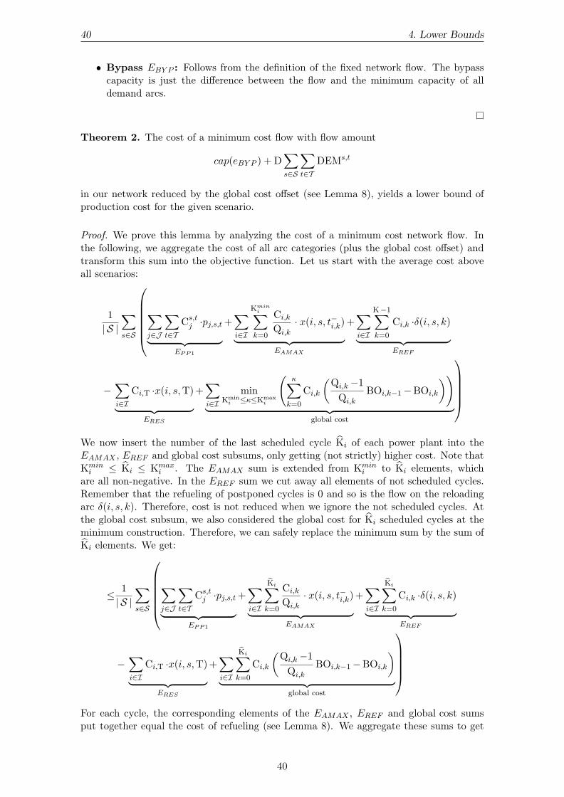
40 4. Lower Bounds

• Bypass EBY P : Follows from the definition of the fixed network flow. The bypasscapacity is just the difference between the flow and the minimum capacity of alldemand arcs.

Theorem 2. The cost of a minimum cost flow with flow amount

cap(eBY P ) + D∑s∈S

∑t∈T

DEMs,t

in our network reduced by the global cost offset (see Lemma 8), yields a lower bound ofproduction cost for the given scenario.

Proof. We prove this lemma by analyzing the cost of a minimum cost network flow. Inthe following, we aggregate the cost of all arc categories (plus the global cost offset) andtransform this sum into the objective function. Let us start with the average cost aboveall scenarios:

1| S |

∑s∈S

∑j∈J

∑t∈T

Cs,tj ·pj,s,t︸︷︷︸

EPP1

+∑i∈I

Kmini∑k=0

Ci,k

Qi,k

· x(i, s, t−i,k)︸︷︷︸EAMAX

+∑i∈I

K−1∑k=0

Ci,k ·δ(i, s, k)︸︷︷︸EREF

−∑i∈I

Ci,T ·x(i, s,T)︸︷︷︸ERES

+∑i∈I

minKmin

i ≤κ≤Kmaxi

(κ∑k=0

Ci,k

(Qi,k−1

Qi,k

BOi,k−1−BOi,k

))︸︷︷︸

global cost

We now insert the number of the last scheduled cycle Ki of each power plant into theEAMAX , EREF and global cost subsums, only getting (not strictly) higher cost. Note thatKmini ≤ Ki ≤ Kmax

i . The EAMAX sum is extended from Kmini to Ki elements, which

are all non-negative. In the EREF sum we cut away all elements of not scheduled cycles.Remember that the refueling of postponed cycles is 0 and so is the flow on the reloadingarc δ(i, s, k). Therefore, cost is not reduced when we ignore the not scheduled cycles. Atthe global cost subsum, we also considered the global cost for Ki scheduled cycles at theminimum construction. Therefore, we can safely replace the minimum sum by the sum ofKi elements. We get:

≤ 1| S |

∑s∈S

∑j∈J

∑t∈T


EPP1

+∑i∈I

bKi∑k=0

Ci,k

Qi,k

· x(i, s, t−i,k)︸︷︷︸EAMAX

+∑i∈I

bKi∑k=0

Ci,k ·δ(i, s, k)︸︷︷︸EREF

−∑i∈I


+∑i∈I

bKi∑k=0

Ci,k

(Qi,k−1

Qi,k

BOi,k−1−BOi,k

)︸︷︷︸

global cost

For each cycle, the corresponding elements of the EAMAX , EREF and global cost sumsput together equal the cost of refueling (see Lemma 8). We aggregate these sums to get

40

4.4. Evaluation 41

the real refueling cost:

=1| S |

∑s∈S

∑j∈J

∑t∈T


EPP1

+∑i∈I

bKi∑k=0

Ci,k ·ri,k︸︷︷︸refueling cost

−∑i∈I


We now extend the sum of refueling costs by all not scheduled cycles. Since ri,k equals 0for these cycles, this does not change the sum. Finally, by moving the refueling costs outof the average above all scenarios, we get the objective function:

=∑i∈I

∑k∈K

Ci,k ·ri,k +1|S|∑s∈S

(∑t∈T

(∑j∈J

Cs,tj ·pj,s,t ·D

)−∑i∈I

Ci,T ·x(i, s,T)

)

4.4 Evaluation

In this section we evaluate the proposed lower bounds. For an introduction of our generalexperimental setup see Chapter 7.

The results that we obtained for all instances can be seen in Table 4.1. Both bounds yieldstable deviations from the best known results. Obviously, the network-based lower boundgives far better results than the auction-based bound. The reason is that the network isdesigned to overcome the disadvantages of the auction (underestimated unit cost of Type-2 power plants and overestimated production capacity). In the flow network, the cost ofproduction by Type-2 power plants is really mapped onto a concrete outage and billedwith the refueling. Furthermore, the network models outages by limiting the productionof the power plants over a certain period of time, while outages are not considered in theauction approach.

Therefore, the remaining gap between the network-based lower bound and an optimalsolution originates mainly from the unconsidered spacing and resource constraints (CT 14- 21) and the caveats against optional outages.

The lower bounds for instances from the sets B and X differ much more from their bestknown solution than instances from the set A do. This probably results from the largernumber of outages and spacing constraints in the respective instances. Consequently, theinfluence of the spacing constraints, which are not modeled in the lower bound, grows andmakes real solutions close to the lower bound hard to obtain.

As the obtained scores (deviation from the best known solution, cf. Section 7.2) of ourlower bounds are similar among the instances from the sets B and X, we assume thatthese instances are somewhat equally hard to solve. Thus, a good solution should alsoyield similar scores for all instances.

41

42 4. Lower Bounds

Auction NetworkInstance Value Score Value Score

A00 8 676 507 008 664 -0,66% 8 701 730 192 910 -0,34%A01 160 847 599 728 -5,13% 165 560 766 563 -2,35%A02 130 148 129 044 -10,09% 139 991 463 398 -4,15%A03 137 744 660 926 -10,80% 148 454 212 611 -3,87%A04 82 428 942 096 -23,45% 102 326 409 223 -8,30%A05 94 379 648 874 -24,99% 112 467 964 426 -10,61%

B06 36 338 357 898 -56,44% 69 592 490 826 -16,58%B07 38 263 622 745 -52,86% 68 528 158 937 -15,58%B08 28 410 840 209 -65,32% 62 594 950 271 -23,60%B09 30 000 446 786 -63,30% 63 991 967 201 -21,72%B10 30 389 023 703 -60,92% 63 747 909 586 -18,03%

X11 33 377 981 846 -57,81% 66 931 120 300 -15,40%X12 36 740 208 840 -52,65% 66 558 720 126 -14,22%X13 25 789 835 024 -66,27% 62 155 964 336 -18,70%X14 26 903 399 271 -64,68% 63 045 557 475 -17,23%X15 28 444 392 103 -62,13% 61 866 985 938 -17,62%

Table 4.1: Lower bounds: We compare both lower bounds with respect to the obtainedobjective function value and its score (deviation from the best known solution,cf. Section 7.2).

42

5. Basic Solution

In this chapter we present a first solution to the proposed problem. Since there is probablyno way to solve even medium-sized instances of this problem exactly in reasonable time,we develop several heuristics. We decompose the problem into an outage scheduling anda power assignment phase. Outage dates hai,k are fixed in the first phase, while powerlevels pj,s,t/pi,s,t and refuelings ri,k are calculated in the second phase for a given outageschedule. Throughout this chapter we primarily care about getting a valid solution –postponing optimization to Chapter 6.

First, Section 5.1 deals with the outage scheduling phase. Due to the large number ofconstraint types (see Section 3.3) and their dependencies we use a CP formulation to finda feasible schedule. In Section 5.2, we present a valid production assignment heuristic fora given set of outages. Therefore, we utilize a demand auction derived from the lowerbound presented in Section 4.2.

In Table 5.1 we give an overview at which point of the solution process we take care of eachconstraint type of the problem. We mark parts of our heuristics with an orange square ifthe consideration of the given constraint is necessary, i.e., not checking this property in theparticular step might result in invalid solutions. A green dot stands for a sufficient mean toachieve this constraint, i.e., after performing this step the remaining solution space cannotfail this constraint.

5.1 Outage Scheduling

In this section we show a heuristic that constructs an outage schedule (i.e., explicit valuesfor all hai,k decision variables) for a given problem instance (see Chapter 3). The resultingschedule is valid with respect to the outage scheduling constraints CT 13 to CT 21. Weadd further constraints to our model, to ensure the feasibility of the remaining productionassignment problem, which is solved in Section 5.2. As Type-1 power plants are notscheduled for outages, we only consider Type-2 power plants here.

We use the constraint programming toolkit Gecode for the creation of outage schedules andtherefore present a suitable CP formulation of our problem in the upcoming sections. TheCP model is presented in a bottom-up approach. In Section 5.1.1.1, we define the differentvariables for a single cycle of a Type-2 power plant and set up their relations among eachother. After that, we establish the relations between consecutive cycles of a power plant inSection 5.1.1.2. Therefore, we also introduce two custom constraints, which propagate fuel

43

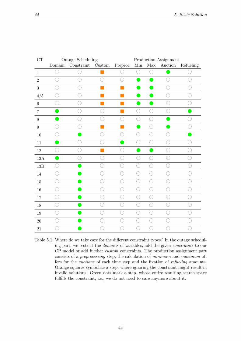
44 5. Basic Solution

CT Outage Scheduling Production AssignmentDomain Constraint Custom Preproc Min Max Auction Refueling

1

2

3

4/5

6

7

8

9

10

11

12

13A

13B

14

15

16

17

18

19

20

21

Table 5.1: Where do we take care for the different constraint types? In the outage schedul-ing part, we restrict the domains of variables, add the given constraints to ourCP model or add further custom constraints. The production assignment partconsists of a preprocessing step, the calculation of minimum and maximum of-fers for the auctions of each time step and the fixation of refueling amounts.Orange squares symbolize a step, where ignoring the constraint might result ininvalid solutions. Green dots mark a step, whose entire resulting search spacefulfills the constraint, i.e., we do not need to care anymore about it.

44

5.1. Outage Scheduling 45

levels between successive cycles and enforce minimum durations of production campaigns.In Section 5.1.3 we model the various outage scheduling constraints, emphasizing the morecomplex constraints that cannot be modelled one-to-one from their definition in Section 3.3.Finally, Section 5.1.4 presents different branching strategies and explains how the searchfor a schedule works.

5.1.1 Basic Modelling

We model all variables using the finite domain integer model provided by Gecode. Notethat problems may arise from the real-valued fuel levels. Hence, when implementing thispart, we have to model fuel level constraints with tolerance for rounding errors.

5.1.1.1 Modelling a single cycle

We start by modeling a single cycle of a Type-2 power plant. The key variable of eachcycle is the decoupling date. Although one variable would technically suffice, we add twoother auxiliary variables for convenience.

Definition 16. Given an arbitrary Type-2 power plant i and cycle k (including the initialcycle −1), we define the boolean-valued finite domain integer variable schi,k as an indicator(1/true if this cycle is scheduled before the end of the time horizon) and an integer-valuedvariable dec∗i,k as the week of decoupling of power plant i in cycle k. Furthermore, we definedeci,k as the result of hai,k. Note that deci,k equals dec∗i,k as long as the cycle is scheduled.Only if a cycle is postponed, the values differ. deci,k then contains the published result−1, while dec∗i,k represents the internally available date range of this outage (which is afterthe time horizon). We set the limits of these variables as follows (remember TOi,k andTAi,k from CT 13):

schi,k ∈ {0, 1} (5.1)

TOi,k ≤ dec∗i,k ≤{

TAi,k if TAi,k 6= −1∞ else

(5.2)

deci,k ∈ {−1, 0, 1, . . . ,W−1} (5.3)

For these three variables we can come up with a basic constraint set, which arises fromCT 13: If the cycle is scheduled, dec∗i,k and deci,k are equal. If it is postponed, deci,k hasto be −1 while dec∗i,k is only limited by TOi,k. Equations 5.4 to 5.6 give a formalizationof this construct:

schi,k ⇐⇒ deci,k = dec∗i,k (5.4)

schi,k ⇐⇒ dec∗i,k < W (5.5)

¬ schi,k ⇐⇒ deci,k = −1 (5.6)

Note that only the deci,k variables need to be assigned in a solution, because they determinethe schi,k variables. The dec∗i,k are unimportant in a solution. Either deci,k equals −1 (i.e.,the cycle is postponed) or it lies in between the earliest and latest allowed decoupling dates.Because the special meaning of deci,k = −1, we do not use deci,k in the following. Insteadwe use dec∗i,k, which is simply not assigned in a solution if the cycle is not scheduled.

The reason for duplicating the decoupling date into the variables deci,k and dec∗i,k is notobvious. But, modeling this way has three advantages:

• Standard Branching: Gecode’s standard branching techniques work towards as-signing all decision variables. In our case we do not care about the specific dateof an outage, if it is scheduled after the time horizon. So, when using a standardbranching, we only consider deci,k as a decision variable.

45


• Smaller Domains: A later cycle is more likely to be postponed (deci,k = −1). So,until we decide if a cycle is scheduled, its domain ranges from −1 to W−1 (scheduledfor the last week), which results in poor constraint propagation. However, dec∗i,kalways represents the true scheduling options.

• Easier Modelling: By using dec∗i,k we can get rid of any exceptions arising frompostponed cycles, when modeling outage dependency constraints (CT 14 to CT 21).Furthermore, this can be seen as a more natural model, since we really move thecycle’s decoupling date after the time horizon.

Although we do not plan any production levels in this phase, it is crucial to track fuel levelsin order to keep the remaining production assignment problem feasible. We give a shortexample: Let us take the minimum achievable fuel level at the beginning of a productioncampaign and the maximum allowed fuel level at the beginning of the next outage. Theirdifference imposes a minimum amount of fuel that has to be consumed during the givenproduction campaign. Since fuel consumption is limited (see PMAXt

i and CT 9), thiseffectively generates a spacing constraint between two successive outages. We model thefuel tracking by three more finite domain integer variables for each cycle:

Definition 17. Given an arbitrary Type-2 power plant i and cycle k (including the initialcycle -1), we define the following variables: prei,k as the fuel level before refueling, refi,k asthe amount of fuel provided during this outage and posti,k as the fuel level after refuelingbut before any production. We set the limits of these variables as follows:

0 ≤ prei,k ≤ AMAXi,k (5.7)

RMINi,k ≤ ref i,k ≤ RMAXi,k (5.8)

0 ≤ post i,k ≤ SMAXi,k (5.9)

The limits of ref i,k can be naturally taken from the bounds of refueling (CT 7). Similarly,we can extract the limits of prei,k and post i,k from the maximum allowed fuel levels beforeand after refueling (CT 11). For the initial campaign we consider post i,−1 = XIi, whileprei,−1 and ref i,−1 can be ignored.

We now add the refueling constraint (CT 10) to our model:

post i,k =Qi,k−1

Qi,k

(prei,k−BOi,k−1) + ref i,k + BOi,k (5.10)

So far, we established a model for a single cycle. Table 5.2 gives an overview of theintroduced variables, their values for the initial cycle (k = −1) and domain boundariesfor the following cycles. In the next section we assemble these cycles to model a completeType-2 power plant.

5.1.1.2 Modelling Type-2 Power Plants

Right now our CP model can handle decoupling dates, scheduled states (i.e., scheduled orpostponed) and fuel levels of each cycle independently. In this section, we first fix the orderof cycles of a Type-2 power plant. Afterwards, we augment our model with constraintsthat guarantee the feasibility of the production assignment problem for a single powerplant in the second phase.

According to CT 13B all cycles of a Type-2 power plant have to be scheduled in the sameorder as they appear in the dataset. Therefore, we introduce Equation 5.11. Note that wedo not need to care if the outage is scheduled, because we use dec∗i,k instead of deci,k.

dec∗i,k+1 ≥ dec∗i,k + DAi,k (5.11)

46


Variablek = −1 k > −1

DescriptionAssign Min Max

schi,k 1 0 1 Is this campaign scheduled?

deci,k 0 −1 W−1 Date of decoupling

dec∗i,k 0 0 ∞ Auxiliary variable for date of decoupling

ref i,k 0 RMINi,k RMAXi,k Amount of fuel provided

prei,k 0 0 AMAXi,k Fuel level before refueling

post i,k XIi 0 SMAXi,k Fuel level after refueling

Table 5.2: Finite domain integer variables instantiated for each cycle of a Type-2 powerplant i. The Initial column comprises the predefined values of this variable forthe initial cycle k = −1, while the Min and Max columns represent the domainlimits for all successive cycles.

Equation 5.11 implies that there is no scheduled outage after the first not scheduled outageof a Type-2 power plant.

Lemma 10. It holds:schi,k+1 = 1 =⇒ schi,k = 1

Proof. We derive this lemma from the previously defined constraints/equations in thissection:

schi,k+1 = 1 5.5⇐⇒ dec∗i,k+1 < W 5.11=⇒ dec∗i,k < W 5.5⇐⇒ schi,k = 1

The constraints provided yet would suffice to create a valid outage schedule for a singleType-2 power plant. Unfortunately, it is not sufficient to guarantee feasible productionassignments later, since we might schedule two outages within a time distance that istoo short to consume enough fuel to comply with CT 11 in the next cycle. Furthermore,from an opposite perspective we discover that fixing two successive outage dates dec∗i,k anddec∗i,k+1 imposes restrictions on the amount of refueling ref i,k.

5.1.2 Additional Constraints

In this section we add constraints to our CP model, which solve the problems shown inthe last paragraph. I.e., they guarantee the feasibility of the production assignment phasefor a yet to find outage schedule. Technically, we have to model further dependenciesbetween the fuel levels and the decoupling dates of consecutive cycles (see Figure 5.1). Onthe one hand, the minimum difference between the fuel levels before (post i,k−1) and after(prei,k) a production campaign imposes a minimum spacing between the decoupling datesdeci,k−1 and deci,k. On the other hand, the maximum distance between the decouplingdates imposes a maximum difference between the fuel levels.

In the following we present a CP formulation in the form of two custom propagators,which enforce the additional constraints. Both propagators heavily rely on the estimationof maximum fuel levels in forward and backward direction in time. Forward propagationworks straightforward (see CT 9). How to perform backward propagation is explained inSection 5.1.2.1. There we show how to deduce an upper bound of the fuel level of a previoustime step from the given fuel level of the present time step. Afterwards in Section 5.1.2.2,

47


deci,k−1

post i,k−1

deci,k

prei,k

Figure 5.1: Conflicting variables of consecutive cycles.

we present a propagator that limits the fuel levels before and after a production cam-paign, based on the possible outage dates. Finally, we present the second propagator inSection 5.1.2.3, which sets up a minimum spacing constraint between consecutive outagesof a plant, considering the fuel levels and dataset parameters.

5.1.2.1 Fuel Level Back Calculation

In this section we present an inverse function that calculates an upper bound of the fuellevel x(i, s, t) from a given future fuel level x(i, s, t+n) and the available production inter-vals in between. This function is utilized in the upcoming additional constraint definitions.Note that the back calculation is easier for time steps t where the fuel level x(i, s, t) is abovethe fuel level threshold BOi,k (see CT 6). In this case we exactly know the maximum pro-duction levels (and with it the maximum possible fuel consumption) of all time steps andcan apply CT 9:

Lemma 11. For an arbitrary Type-2 power plant i and a given fuel level at time stept+ 1 we can bound the fuel level at time step t as:

x(i, s, t) ≤ x(i, s, t+ 1) + PMAXti ·D

Note that Lemma 11 holds for all time steps. As long as the production level is notimposed, this bound even guarantees that future fuel limits are achievable if the currentfuel level does not exceed its bound. To give this guarantee while BOi,k is under-runrequires additional effort. We do not know the available ratio of the maximum productionlevel (see Figure 5.2), because it depends on the previous fuel level – the value we arelooking for. From CT 6 and CT 9 we derive:

x(i, s, t) = x(i, s, t+ 1) + PBi,k(x(i, s, t)) · PMAXti ·D (5.12)

To transform this equation into a computable upper bound, we first introduce an alterna-tive notation of PBi,k. While the original problem defines this piecewise linear function byits data nodes (fuel level, ratio), we use a different representation to ease the calculation:

Notation 1. Let the imposed power profile PBi,k : R≥0 → [0, 1] for a Type-2 power planti and cycle k be denoted as follows. Let s0, s1, . . . , sn denote the fuel level values of thedata nodes in descending order (i.e., s0 = BOi,k and sn = 0). Besides, let ml denote theslope of the ratio between sl and sl−1 and nl denote the offset of this linear function (seeFigure 5.2). For a given fuel level x less or equal s0 we calculate the available fuel ratio byPBi,k(x) := ml · x+ nl where l is chosen such that sl ≤ x < sl−1. Furthermore, we definem0 := 0 and n0 := 1 so that, for x ≥ s0 it holds PBi,k(x) = 1.

By using Notation 1 we can rewrite Equation 5.12:

48


ratio= m l

· fuel + n l

BOi,k = s0

PBi,k

0fuel level

1

0

avail. ratioof PMAXt

iconsumption

s0sl−1slsn−1

Figure 5.2: Available production ratio during a time step in relation to the current fuellevel. As long as there is more than BOi,k fuel, we can choose the ratio freely(yellow area). Otherwise the ratio is fixed by the piecewise linear concavefunction PBi,k. Note that we ”move” left in this chart, since we consume fuelbetween two time steps.

Lemma 12. For an arbitrary Type-2 power plant and a given fuel level at time step t+1,there exists an l such that we can bound the fuel level at time step t to:

x(i, s, t) ≤ x(i, s, t+ 1) + (ml · x(i, s, t) + nl) · PMAXti ·D (5.13)

and it holds sl ≤ x(i, s, t) < sl−1.

By solving Lemma 12 for x(i, s, t) we can present the core of the inverse function, whichworks out the initial fuel level of a time step.

Lemma 13. For an arbitrary Type-2 power plant i with a fuel level x(i, s, t + 1) at theend of time step t, we can limit the fuel level x(i, s, t) at the beginning of this time step.There exists a (not necessarily unique) l such that

x(i, s, t) ≤ x(i, s, t+ 1) + PMAXti ·D ·nl

1− PMAXti ·D ·ml

and sl ≤ x(i, s, t) < sl−1 or production during t was unbound (x(i, s, t) ≥ BOi,k).

Proof. We assume that production is bound, i.e., x(i, s, t) < BOi,k (otherwise the equationcan be reduced to Lemma 11). The existence of an l that fulfills sl ≤ x(i, s, t) < sl−1 followsdirectly from Notation 1. Taking a suitable l, we can transform Lemma 12 into the soughtformula.

Although we know that a suitable segment l exists, it is not trivial to forecast. A goodchoice might be the segment of the x(i, s, t + 1) value, but dependent on the granularityof PBi,k the segment of x(i, s, t) might still be several steps away. Algorithm 3 takes asimpler approach, iterating over all segments of PBi,k and stopping at the first matchingsegment – thus maximizing the available production ratio.

Finally, note that our back calculation does generally not provide a lower bound of thefuel level before production in cases where the residual fuel level is so low that productionmight have been ceased for several time steps (see CT 6). In this case we cannot determinethe last time step of production.

49


Algorithm 3: PREVIOUS (plant i, time step t, power profile PBi,k, fuel level post)Input: Plant parameters and fuel level after production of time step tOutput: Upper bound on the fuel level before production of time step tbegin

l←− 0// Loop over segments, stop at the first matching segmentrepeat

l←− l + 1// Perform calculation of Lemma 13pre ←− (post + PMAXt

i ·D ·nl)/(1− PMAXti ·D ·ml)

until sl ≤ prereturn pre

end

5.1.2.2 Fuel Level Propagation

In this section we model the connection between fuel levels of consecutive cycles, specificallythe difference between the level after refueling post i,k and the level before the refuelingof the next campaign prei,k+1. We focus on the estimation of the amount of productionduring the campaign. Technically, we realized this section by adding a custom propagatorto the CP model. We show the concept of this propagator, while omitting implementationspecific details.

In our CP model fuel levels of consecutive cycles are not related yet. But, since thesefuel levels effectively impose spacing constraints between outages, we cannot ignore themhere. From the problem formulation we know that fuel levels depend on production levels(CT 9). Besides, other constraints apply during a production campaign, for example, theallowed maximum modulation (CT 12) or power profile imposition (CT 6) if we under-runthe threshold BOi,k.

When modeling the overall production of a campaign, the following degrees of freedomarise from the problem formulation:

• start of production campaign (dec∗i,k + DAi,k)

• opening fuel level (post i,k)

• end of production campaign (dec∗i,k+1 or time horizon)

• final fuel level (prei,k+1)

• maximum modulation (MMAXi,k)

To limit the fuel level variables we consider a minimum and a maximum production sce-nario. Maximum production is obviously done with PMAXt

i. Similarly we model minimumproduction by adding the maximum modulation MMAXi,k to the fuel level and by per-forming maximum production at all time steps. This works because the accumulateddifference between the maximum and minimum production cannot exceed MMAXi,k. Onemight imagine these additional units of fuel as no-production units, which, when consumedby a plant, reduce the plant’s real production level.

In the following we introduce the forward and the backward propagation of this constraint.First, we limit the opening fuel level of the next cycle prei,k+1 by performing a maximumand minimum production starting with post i,k (Forward Propagation). After that wesimulate maximum production starting with prei,k+1 and going back in time (BackwardPropagation), thus finding an upper bound of post i,k for any feasible production assignmentproblem.

50


Forward Propagation

Since we want to constrict prei,k+1 as much as possible, we have to choose the concretevalues from the remaining degrees of freedom accordingly. To reach the maximum finalfuel level we take the upper domain limit of the opening fuel level, choose the shortestduration of the production campaign and fully exhaust modulation. Contrary, to reachthe minimum final fuel level we take the lower domain limit of the opening fuel level,choose the longest duration and no modulation. Table 5.3 gives an overview of the usedparameters, while Figure 5.3 illustrates the process.

Minimum Maximum

start min(dec∗i,k) + DAi,k max(dec∗i,k) + DAi,k

end max(dec∗i,k+1) min(dec∗i,k+1)

fuel min(post i,k) max(post i,k)

modulation 0 MMAXi,k

Table 5.3: Forward propagation parameters to get an upper limit (Maximum) and lowerlimit (Minimum) of prei,k+1.

fuel

timedec∗i,k + DAi,k dec∗i,k+1

post i,k

prei,k+1

MMAXi,k

Figure 5.3: Forward propagation: From post i,k we simulate maximum production (lowerline) and minimum production (upper line) to limit the domain of prei,k+1.

Both maximum and minimum calculation can be performed using CT 9 for all time stepsof the considered campaign range and initializing the first fuel level properly.

Backward Propagation

While the forward propagation of fuel levels can be seen just as completion of the CPmodel, backward propagation is crucial to keep the production assignment problem of thenext phase feasible. Assuming that post i,k would not be limited this way, we might loadmore fuel than can be consumed in the following production campaign and fail to reachthe maximum allowed fuel level before refueling of the next campaign AMAXi,k+1 (seeCT 11). Technically, we can also provide a lower bound for post i,k, but this is not a hardconstraint, since less fuel would just result in ceased production of this plant.

Backward propagation should constrict post i,k, so we again have to choose values from theremaining degrees of freedom (see Table 5.4). To determine the maximum allowed fuellevel at the beginning of the production campaign we take the upper domain limit of thefinal fuel level, choose the longest duration of the production campaign and no modulation.

51


Minimum Maximum

start min(dec∗i,k+1) max(dec∗i,k+1)

end max(dec∗i,k) + DAi,k min(dec∗i,k) + DAi,k

fuel min(prei,k+1) max(prei,k+1)

modulation MMAXi,k 0

Table 5.4: Backward propagation parameters to get an upper limit (Maximum) and lowerlimit (Minimum) of post i,k.

fuel


post i,k

prei,k+1

MMAXi,k

Figure 5.4: Backward propagation: From prei,k+1 we simulate backward maximum pro-duction (upper line) and backward minimum production (lower line) to limitthe domain of post i,k. Note that the minimum production is more of a sugges-tion than a hard constraint.

For the sake of completeness Table 5.4 also lists the parameters to get a lower limit of a”useful” post i,k. Again Figure 5.4 illustrates the process.

Both maximum and minimum calculation can be performed using Algorithm 3 for all timesteps of the considered campaign range in descending order and initializing the last fuellevel properly.

5.1.2.3 Outage Date Propagation

In the last section we limited the fuel levels before (post i,k) and after (prei,k+1) a productioncampaign. Given these levels and the power plant’s maximum production for all time stepsof the production campaign, we can deduce the minimum period of time the plant needsto consume this fuel difference. Note that scheduling the neighboring outages in a shorterdistance would not yet fail our outage scheduling phase but surely result in an infeasibleproduction assignment problem.

In this section we set up a spacing constraint between consecutive outages of a given Type-2 power plant. Similar to the last section, we simulate maximum production (in forwardand backward direction) to constrain the latest start and earliest stop date of a productioncampaign. Again, we realized this as a custom propagator in Gecode, while this documentjust shows the concept.

Contrary to the fuel propagation constraint, there are no real degrees of freedom in thisconstraint. The considered fuel levels can be fixed (minimum before and maximum afterproduction), while production itself is always assumed to be maximal. Only the decouplingdates are variable.

52


During forward propagation we determine the earliest possible stop date of a productioncampaign (or the earliest date of decoupling of the next campaign, respectively). Therefore,we try to reach the maximum fuel level at the end as early as possible, which means:starting at the earliest date of coupling and performing maximum production. Figure 5.5illustrates this concept.

fuel


min(post i,k)

max(prei,k+1)

Figure 5.5: Outage Forward Propagation: Starting maximum production at the earliestpossible date with the minimum fuel level (min(post i,k)), we can limit theearliest date of the next outage to the time step, where we reach the maximumallowed fuel level at the end (max(prei,k+1)).

Backward propagation works in a similar way and is illustrated in Figure 5.6. We arelooking for the latest possible start date of a production campaign. We assume thatproduction reaches the maximum allowed fuel level before refueling AMAXi,k+1 at thelatest possible time step, while maximum production has been performed throughout thewhole production campaign. The time step where the fuel level back calculation reachesthe minimum pre-production fuel level is an upper bound for the coupling date.

fuel


min(post i,k)

max(prei,k+1)

Figure 5.6: Outage Backward Propagation: Assuming maximum production until thelatest possible date, reaching the maximum allowed fuel level at the end(max(prei,k+1)), we can limit the latest date of the beginning of the produc-tion campaign to the time step where we reach the minimum fuel level beforeproduction (min(post i,k)).

5.1.3 Modelling Constraint Types

In the last section we worked out a basic model of Type-2 power plant operations that caresfor feasibility of the second phase – the production assignment. All constraints considered

53


yet (CT 3 - 13) applied to a single power plant. In this section we model the remainingconstraints CT 14 - 21.

Note that CT 14 - 18 are all spacing constraints with large similarities. In Section 5.1.3.1we first show how to formulate these spacing constraints for our CP model. After that,the constraints CT 19 -21 are handled separately in Sections 5.1.3.2 to 5.1.3.4, because allof them are special on their own.

5.1.3.1 Handling Spacing Constraints

The spacing constraints CT 14 - 18 operate on a set A of Type-2 power plants. For allpairs of cycles k and k′ from two different power plants i and i′ in A they impose a certainminimum spacing between these cycles’ outages. We can transform the constraints fromtheir definition in Section 3.3.3.1 in a canonical way and add them to our model for allpairs of cycles from different Type-2 power plants :

[CT 14] Minimum spacing between outages(dec∗i,k− dec∗i′,k′ −DAi′,k′ ≥ Se

)∨(

dec∗i′,k′ − dec∗i,k−DAi,k ≥ Se)

[CT 15] Minimum spacing between outages during a specific period

(ID−DAi,k < dec∗i,k) ∧ (dec∗i,k ≤ IF) ∧ (ID−DAi′,k′ < dec∗i′,k′) ∧ (dec∗i′,k′ ≤ IF)

=⇒ (dec∗i,k− dec∗i′,k′ −DAi′,k′ ≥ Se) ∨ (dec∗i′,k′ − dec∗i,k−DAi,k ≥ Se)

[CT 16] Minimum spacing between decoupling dates

| dec∗i,k− dec∗i′,k′ | ≥ Se

[CT 17] Minimum spacing between coupling dates

| dec∗i,k + DAi,k− dec∗i′,k′ −DAi′,k′ | ≥ Se

[CT 18] Minimum spacing between decoupling and coupling dates

| dec∗i,k + DAi,k− dec∗i′,k′ | ≥ Se

Note that we do not need to care if the cycles are scheduled or not, since we always usethe dec∗i,k variables. If a cycle may not be scheduled, the upper bound of dec∗i,k is infinityand therefore all the just formulated constraints hold.

5.1.3.2 [CT 19] Resource Constraint

To model this constraint type we make use of the cumulatives constraint (see [BC02])of Gecode, which schedules tasks onto limited resources. In our setup we have a singleconstrained resource per instance of CT 19 and a task corresponds to the usage of thisresource during an outage. Note that the outage’s duration and the time of resourceconsumption are not equal – resource consumption starts Li,k weeks after decoupling andlasts for TUi,k weeks. Therefore, we have to calculate the dates for each task relative tothe decoupling date of each outage. We have to set the start and duration of each task,where starti,k is again a finite domain integer variable while durationi,k is a constant. Theheight is set to 1 for each task, since CT 19 states that each outage consumes exactly oneunit of the resource.

54


The global resource limit is given as Q and can be used directly. Algorithm 4 gives apseudo-code notation of the approach stated above.

Algorithm 4: POST#19 (A, starts L, durations TU, limit Q)

beginforeach i ∈ A do

foreach k ∈ K dostarti,k ←− dec∗i,k +Li,kdurationi,k ←− TUi,k

heighti,k ←− 1

cumulatives(start, duration, height,Q)end

5.1.3.3 [CT 20] Maximum number of outages during a given week

We model this constraint type utilizing a linear constraint. A boolean-valued FDI vectormarks if an outage takes place during the given week. The sum of this vector is limited tothe given number of maximum parallel outages. See Algorithm 5.

Algorithm 5: POST#20 (A,week H, limit N)

beginv ←− vector of boolean-valued FDI variablesforeach i ∈ A do

foreach k ∈ K do(dec∗i,k ≤ H) ∧ (dec∗i,k + DAi,k > H)⇔ vi,k = 1

linear(v, IRT LQ,N)end

5.1.3.4 [CT 21] Maximum offline power capacity during a specific period

Similarly to CT 20 we use a linear constraint here. But instead of limiting the sum of thevector itself, we limit the sum of v · PMAX, hence limiting the maximum power capacityon outage. Since this constraint applies over a certain period of time, we have to postthis constraint for each time step in between. Although outage dates only vary in weeks,posting one constraint per week would not suffice, since the maximum capacity of a Type-2power plant can change during a week. See Algorithm 6.

Algorithm 6: POST#21 (A,weeks [ID, IF], limit IMAX)

beginforeach ID ≤ time step t ≤ IF do

v ←− vector of boolean-valued FDI variablesforeach i ∈ A do

foreach k ∈ K do(dec∗i,k ≤ weekt) ∧ (dec∗i,k + DAi,k > weekt)⇔ vi,k = 1

linear(v,PMAXt, IRT LQ, IMAX)

end

5.1.4 Branching

The employed branching strategy is not crucial to find any solutions, but important tofind good solutions fast. As introduced in Section 2.1.4 branching always consists of twoparts: choosing an unassigned variable and deciding what to do with it.

55


The constraints set up now limit all variable domains as strong as possible. When prop-agation reaches a fix point (i.e., no further domain limiting is possible), we have to addfurther constraints and branch the resulting search space, to allow further constraint prop-agation. Branching and propagation are alternating steps. We repeat them until all cyclesare either scheduled at a specific date or postponed.

In this section we present three different branching strategies and show their respectiveadvantages and disadvantages. The first two are standard Gecode branchings. Rememberthat we designed our model in a way (deci,k vs. dec∗i,k) that standard branchings work forour needs.

The first branching strategy, presented in Section 5.1.4.1, schedules outages with the small-est domain first. Our second branching strategy introduces a randomized approach inSection 5.1.4.2. Finally, a branching that schedules outages in the order in which theyappear is presented in Section 5.1.4.3, overcoming a problem of the branchings before: thedecision to postpone all optional outages.

No matter which branching technique we use, searching the whole search tree is out ofscope. Even if we assume that we only try out the lower and upper date bounds ofeach outage, the search space is still of size 2|outages|. However, medium sized datasetshave around 60 outages to be scheduled (the biggest ones have around 300). Therefore,randomizing the search and continuously limiting of the domains towards promising regionsshould yield good options to achieve cheap schedules.

In Chapter 6 we develop more sophisticated branching techniques to improve the resultsfound. This includes branchings augmented with lower bound data.

5.1.4.1 Smallest Domain Branching

In our first shown branching technique we fix the outages with the smallest domain first,i.e., outages with a small difference between max(dec∗i,k) and min(dec∗i,k). Although wedo not care for the cost incurred this might be reasonable to find first solutions. Outageswith small domains are more likely to become infeasible if other outages are assigned first.

Choosing a good value is not simple: if an outage is scheduled too early we loose fuelduring the outage’s refueling, but if the outage is scheduled too late we run out of fueland are effectively offline longer than necessary. Since we set up constraints that ensurefeasible fuel levels, we keep this branching simple and choose from three options: minimum,median, maximum decoupling date.

branch(dec, INT VAR SIZE MIN, INT VAL MIN)

branch(dec, INT VAR SIZE MIN, INT VAL MED)

branch(dec, INT VAR SIZE MIN, INT VAL MAX)

5.1.4.2 Random Branching

Although deterministic branching would sooner or later explore all possible solutions, ithas the huge disadvantage that we are nearly unable to revoke early decisions, due to thesize of our search tree. To overcome this problem we present a randomized branching inthis section, which chooses an outage and the assigned value randomly from all unassignedoutages and their respective domains.

Choosing outage dates randomly often results in infeasible spaces. Therefore, we restartthis branching frequently, at the latest when a solution has been found. Especially the

56

5.2. Production Assignment 57

decision to schedule or postpone a specific cycle often leads to this problem because wecannot predict if the resulting spacing constraints can be fulfilled. Therefore, we use apreprocessing before applying this branching:

1. perform an initial propagation step

2. postpone all cycles whose sch-variable’s domain contains 0

This way we only schedule the mandatory cycles, which results in less constraints andless failed spaces. Unfortunately, this also results in poor solutions for weak constraineddatasets, since here most cycles are optional, but not scheduling them leads to Type-2power plants running out of fuel.

branch(dec, INT VAR RND, INT VAL RND)

5.1.4.3 Sweep Branching

Remember that the quality of a branching can be seen as how early infeasible regions aredetected. Both previously presented branchings fail from this point of view, because thecycles assigned one after another are seldom closely related. This results in situationswhich look feasible until we try to assign a cycle, whose predecessor and successor havealready been assigned. For this reason it might be useful to assign variables of similardates consecutively, as this might result in early detection of failed states and thereforefinding more results in the given time.

Our third proposed branching overcomes this problem. It always chooses the cycle thatminimizes min(dec∗i,k) and assigns dec∗i,k to its minimum. So, when scheduling a cycle,we can be sure that its previous cycle has already been scheduled to a fixed date. If theminimum above all unassigned dec∗i,k is behind the time horizon, i.e., greater or equal W,the remaining cycles are not scheduled.

5.2 Production Assignment

In this section we present a power assignment heuristic derived from the auction-basedlower bound presented in Section 4.2. Power assignments are performed for a given outageschedule (i.e., all hai,k are fixed) and assign the resulting decision variables: productionlevels pj,s,t/pi,s,t and refueling amounts ri,k. We use the same auction method and Type-1power plant offers as presented in Chapter 4 about lower bounds but augment the offers ofType-2 power plants by their current fuel level and consumed modulation (i.e., the differ-ence between the maximum and realized production throughout the current campaign).

The auction is run in ascending order of the time steps and for all scenarios in parallel.This way, it is easy to adjust the fuel levels from the previous time step and fix the refuelingamounts consistently, when we run the auction for the second time step of an outage.

This chapter is organized as follows. First, we present a special preprocessing step in Sec-tion 5.2.1 which is performed for each Type-2 power plant to ensure production feasibility.After that we show how the offers of each Type-2 power plant are compiled in Section 5.2.2.Finally, we introduce the calculation of the refueling amounts in Section 5.2.3.

Although cheap production is the ultimate goal, sometimes we have to utilize a Type-2power plant at any cost to comply with the given constraints. Fortunately, the provideddatasets suggest that Type-2 power plant production is generally cheaper than Type-1power plant production. But, this is nowhere stated explicitly and cannot be taken forgranted. Nevertheless, we assume in this chapter that it is desirable for each Type-2 power

57


plant to produce as much as possible and adjust our refueling strategy accordingly. Thismeans that we always choose the maximum possible refueling amount and thus increaseType-2 power plant utilization. A more sophisticated refueling strategy is presented inSection 6.6.

5.2.1 Type-2 Power Plant Preprocessing

During each production campaign a certain amount of fuel has to be consumed to reachthe fuel level limits that apply before or after the upcoming refueling (see CT 11). InSection 5.1.2.2 we introduced a custom constraint that assured this property betweensuccessive outages. In this preprocessing step we define this limit for each time step,relying on the custom constraint that the assignment problem is feasible.

We start at the last time step and move backward in time. Since we know all outage dates,we can assign a maximum allowed fuel level to each time step by assuming maximumproduction in each step and minimum refueling during each outage. See Algorithm 7 fora pseudo-code illustration of this preprocessing step.

Note that these maximum fuel levels impose a minimum production if the current fuellevel comes close to its maximum.

Algorithm 7: PREPROCESS (plant i)Output: Vector of upper bounds of fuel levels after production for each time stepbegin

// initialize the last element of the result vectorfuelmaxT ←−∞foreach scheduled k ∈ K in descending order do

// backward propagation of the maximum fuel levelfor t = t+i,k − 1 to t∗i,k do

fuelmaxt ←− PREVIOUS(i, t, fuelmaxt+1)// apply fuel level limit after refuelingfuelmaxt−i,k+1 ←− min(max(post i,k), fuelmaxt∗i,k)

// reconstruct the fuel level before a minimum refueling

fuelmaxt−i,k←−

Qi,k

Qi,k−1(fuelmaxt−i,k+1 −min(ref i,k)− BOi,k) + BOi,k−1

// apply fuel level limit before refuelingfuelmaxt−i,k

←− min(max(prei,k), fuelmaxt−i,k)

return fuelmaxend

5.2.2 Type-2 Power Plant Offers

Besides the maximum allowed fuel levels, we have to take care of several other constraintswhen assembling the offered production amounts of a Type-2 power plant. Firstly, offershave to comply with imposed power profiles if we under-run the fuel level threshold BOi,k.This is achieved by setting an imposed power level as the minimum offer. Since we trackthe fuel level of each time step, we can easily calculate this production level. Secondly, themaximum modulation over each cycle has to be respected. Since the auction should bedone in ascending order of the time steps, the production levels of previous time steps areknown, and with them the currently consumed modulation. Given the maximum allowedfuel levels of each time step, we can now formulate the offers.

58

5.2. Production Assignment 59

Type-2 Power Plant Minimum Offers

Minimum offers ensure the validity of the found assignment. Therefore, we consider thefollowing constraints here:

CT 6: If the power level is imposed, we calculate the exact level and set it as the minimumoffer.

CT 11: If the current fuel level exceeds the maximum allowed fuel level of this time step,we are not able to reach the maximum fuel level before or after refueling of the nextcycle. Therefore, we set a minimum offer, such that the fuel level is reduced to itsmaximum allowed value.

CT 12: If the consumed modulation of the current cycle (including the time step of theauction) would exceed the allowed maximum modulation, the minimum offer is set,such that the modulation equals MMAXi,k.

Algorithm 8 gives a pseudo-code notation of this process.

Algorithm 8: MINOFFER (plant i, cycle k, scenario s, time step t)Output: Minimum required amount of productionbegin

amount←− 0// Is this a production time step? [CT3]if t∗i,k ≤ t then

// Imposed power profile active? [CT6]if fuelleveli,t < BOi,k then

amount←− PBi,k(fuelleveli,t) · PMAXti

else// Stay below maximum fuel level [CT11]if fuelleveli,t > fuelmaxi,t then

amount←− (fuelleveli,t − fuelmaxi,t)/D

consumed modulation =∑t

τ=t∗i,k(PMAXτ

i −p(i, s, τ)) ·D// Stay below maximum modulation [CT12]if consumed modulation > MMAXi,k then

amount←− max(amount, (consumed modulation−MMAXi,k)/D)

return amountend

Type-2 Power Plant Maximum Offers

Determining the maximum offers is easy. For time steps where a Type-2 power plant isoffline or its production is imposed, the maximum production was already set by the mini-mum offer. During all other time steps, the only constraints limiting maximum productionare CT 4, stating the maximum production of the plant, and CT 9, limiting the fuel levelto non-negative values. Algorithm 9 assembles the maximum offered production amount.

5.2.3 Refueling Amounts

Finally, we have to decide how much fuel to reload during each outage. If the auction isrun for a time step in which a refueling for plant i has to be performed, we know i’s currentfuel levels in all scenarios, because the previous auctions have already been executed. Sincewe calculated the maximum allowed fuel levels of all scenarios in the preprocessing step,we can determine a possible refueling interval for each scenario. The intersection of theseintervals is the globally possible refueling interval of the considered outage.

59


Algorithm 9: MAXOFFER (plant i, cycle k, scenario s, time step t)Output: Maximum available amount of productionbegin

amount←− 0// Is this a production time step? [CT3]if t∗i,k ≤ t then

// production not imposed? [CT6]if fuelleveli,t ≥ BOi,k then

// choose minimal upper bound from [CT4/5] and [CT9]amount←− min(fuelleveli,t/D,PMAXt

i−p(i, s, t))return amount

end

Lemma 14. Given an arbitrary Type-2 power plant i and cycle k, the intersection of thescenarios’ refueling intervals ri,k is not empty.

Proof. Since the realized fuel level in each scenario is less or equal its upper bound foundin the preprocessing step, we can at least perform a minimum refueling without exceedingthe maximum allowed fuel level of the next time step (see Algorithm 7).

We still have to decide which value to take from the global refueling interval of the outage.A higher amount of refueling probably results in higher utilization of the plant. Thisseems desirable, as the provided instances suggest that Type-2 power plant production isgenerally cheaper than production by Type-1 power plants. On the other hand, a largerrefueling results in more residual fuel and thus a worse refueling difference, i.e., more lostfuel during refueling (see CT 10).

For now, we always choose the maximum possible refueling amount and postpone opti-mization to Section 6.6. Algorithm 10 demonstrates the calculation of the concrete value.

Algorithm 10: REFUELING (plant i, cycle k, time step t)Output: The reloading amount to performbegin

a←− RMAXi,k

foreach scenario s doa←− min

(a, fuelmaxi,t−i,k+1 − BOi,k−Q−1

Q (fuellevels,t−i,k − BOi,k−1))

return aend

5.3 Evaluation

In this section we present the first results of our approach. We evaluate the proposedbranching strategies with respect to the solution quality. As the ROADEF/EURO Chal-lenge 2010 limits program running times to 30 minutes (for A instances) and 60 minutes(for B and X instances), we always exploit this time. Thus, deterministic branchings(smallest domain branching, sweep branching) iterate through the CP solutions (i.e., out-age schedules) and run the production assignment phase for each found schedule, alwayskeeping the best solution. Contrary, random branching is restarted from the root of thesearch tree after it visited a certain number of failed spaces. As this maximum failurecount, we choose twice the number of outages to assign. This number is big enough to

60

5.3. Evaluation 61

outage scheduling

set up model

initial reasoning

postpone optional cycles

run search

production planning

fuel preprocessing

greedy heuristic

offers refueling

greedy heuristic

offers refuel

update best result

instance

resultouta

gesc

hedu

le

restart/proceed until time limit

Figure 5.7: Illustration of the overall solution process. Postpone optional cycles is notapplied when using sweep branching. Additionally, only random branchingrestarts the search from the beginning, while both other branchings iterate tothe next solution.

ignore single failures and small enough to restart soon if it seems we search an infeasibleregion of the search tree. If the CP yields a valid outage schedule, we run the productionassignment phase for the found schedule and also restart the CP from its root. See Fig-ure 5.7 for an illustration of the overall process. All three presented branching techniqueshave very low computational overhead, as their choice depends solely on the domains ofthe decision variables (dec∗i,k). For an introduction of our general experimental setup andthe evaluated instances see Chapter 7.

Let us first have a look at the results of smallest domain branching. We evaluate all threeoptions: minimum, median, maximum branching. The results obtained for all instancescan be seen in Table 5.5. For most instances we get a fair score (the deviation from thebest known solution, see Section 7.2 for a precise definition), with exceptions for the lessconstrained instances B08 and B09.

In 6 of 48 cases the branching was not able to find a solution in the given time. We supposethat in these cases an infeasible variable assignment was made early by the branching andthere was not enough time to backtrack up to this point. As smallest domain branchingworks deterministic, repeating the experiment does not improve the situation.

Note that 9 of 15 best solutions have been obtained using the median value strategy.This is comprehensible, since neither very early nor very late decoupling dates are desired.Scheduling an outage too early leads to large amounts of residual fuel and more expensiverefueling (cf. CT 10), while too late outages result in Type-2 power plants running out offuel. There are also three (two) instances where late (early) branching outperforms theother strategies. In these cases, other factors like the number of parallel outages or thecurrent unit cost of other power plants might influence the result stronger than the plants’fuel levels. Finally, we cannot generally say that it is good to schedule outages after acertain proportion of their available decoupling interval.

The second analyzed technique is random branching. Compared to both other branchingsit provides pretty good results. We attribute this to the fact that our random branch-ing is restarted regularly and therefore visits many more different regions of the searchtree. Unfortunately, this technique fails quite often to find a feasible outage schedule (seeTable 5.6). This means, we waste a lot of time evaluating ”dead” parts of the search tree.

As repeated random branching results in different outage schedules, we analyze again ifthere is a promising direction of decoupling dates (i.e., early or late). Therefore, we sum

61


Instance MIN MED MAX

A00 0.16% 0.19% 0.12%A01 2.11% 1.03% 0.56%A02 2.37% 0.89% 0.96%A03 1.96% 1.41% INFEASIBLEA04 2.54% INFEASIBLE 3.27%A05 INFEASIBLE INFEASIBLE INFEASIBLE

B06 9.93% 10.01% 13.86%B07 18.52% 12.68% 11.57%B08 4 716.79% 4 647.15% 4 805.49%B09 4 605.46% 4 027.56% 4 224.70%B10 11.45% 9.53% 9.94%

X11 10.35% 7.01% 7.89%X12 10.57% 6.82% 8.27%X13 14.37% 11.23% INFEASIBLEX14 18.75% 12.65% 15.66%X15 9.38% 6.87% 6.51%

Table 5.5: Smallest Domain Branching: We compare the achieved scores (deviations fromthe best known results, cf. Section 7.2) by the strategies MIN, MED and MAXfor all proposed instances. The best results are in bold font. Runs that didnot give a valid solution in 30 minutes (set A) or 60 minutes (set B and X) aremarked as infeasible.

Instance Best Score Iterations Failure Rate

A00 0.12% >1000 0%A01 0.37% >1000 8%A02 0.61% >1000 30%A03 0.71% >1000 17%A04 1.83% 909 28%A05 2.26% >1000 64%

B06 8.16% 176 23%B07 9.39% 178 12%B08 4 554.66% 71 30%B09 3 840.82% 66 20%B10 8.25% 59 12%

X11 6.54% 217 37%X12 6.04% 230 29%X13 10.29% 189 65%X14 12.00% 84 44%X15 5.61% 90 28%

Table 5.6: Random Branching: We show the best achieved score (cf. Section 7.2) for allinstances. Column iterations lists the number of restarts of our search procedureduring the given time. Failure rate lists the proportion of iterations that didnot provide a valid result before the next restart.

62

5.3. Evaluation 63

Instance A0

185

200

0.130 0.155

date

sum

Instance A1

9200

9500

0.40 0.65

Instance A2

16300

16800

0.65 0.95Instance A3

score in %16900

17400

0.70 0.90

date

sum

Instance A4

score in %28500

29700

1.9 2.6

Instance A5

score in %

26300

27800

2.5 6.5

Figure 5.8: Random Branching: Results from around 1000 iterations on the A instances.We plot the sum of decoupling dates (not scheduled outages are set to W)against the obtained score (cf. Section 7.2). The higher the sum of decouplingdates the later the outages have been scheduled.

up all single decoupling dates and add a dummy value of W (number of weeks in theinstance) for each not scheduled outage. This way, a higher sum can be interpreted asscheduling outages at a later date. The results are plotted in Figure 5.8.

Although there seem to be trends for each instance, these trends vary heavily. Later datesgive better results for instance A1. Contrary, earlier dates provide cheaper schedules forinstance A5. There is even one instance – A4 – without a clear trend. Note that theseresults coincide with the results obtained from smallest domain branching.

Next, we look at the results of sweep branching (see Table 5.7). Although it does generallynot perform as well as random branching, we note that it is the only technique providingreasonable results for all instances. Its main advantage is that we can postpone the decisionwhich outages/cycles we want to schedule and which not. Furthermore, this techniquebranches into very little failed spaces, since the decision variables are assigned in ascendingorder (i.e., dec∗i,k before dec∗i,k+1). This is the same order in which these variables dependon each other and therefore, each decision immediatelly takes effect on all the ”later”variables of a plant. This results in better propagation and thus less failed spaces.

Finally, we compare the results of all three branching techniques in Table 5.7. We no-tice that 14 out of 16 best results have been obtained using random branching. Both,smallest domain branching and random branching, fail at instances B08 and B09. Theseinstances have a lot of optional cycles, which are not scheduled by these branchings. Sweepbranching solves these instances much better, since optional cycles are only not scheduledif they become impossible cycles while searching. Therefore, we will put further effort intodetermining promising decoupling dates.

63


Instance Domain Random Sweep

A00 0.12% 0.12% 0.16%A01 0.56% 0.37% 2.12%A02 0.89% 0.61% 2.34%A03 1.41% 0.71% 1.95%A04 2.54% 1.83% 2.50%A05 INFEASIBLE 2.26% 6.54%

B06 9.93% 8.16% 11.53%B07 11.57% 9.39% 16.53%B08 4 647.15% 4 554.66% 17.88%B09 4 027.56% 3 840.82% 27.90%B10 9.53% 8.25% 11.90%

X11 7.01% 6.54% 10.57%X12 6.82% 6.04% 10.58%X13 11.23% 10.29% 14.86%X14 12.65% 12.00% 20.43%X15 6.51% 5.61% 9.94%

Table 5.7: Overview of the three basic branching techniques: smallest domain branching(Domain), random branching (Random) and sweep branching (Sweep). Weshow the best scores for all instances achieved by each branching.

64

6. Optimization

From the last chapter we learned that the considered search spaces are far too big to befully explored. Thus, it is not satisfactory to rely on the current model and basic branchingtechniques to receive good results. In this chapter we examine strategies that provide morepromising outage schedules and improve production assignment.

In the first three sections, we focus on the branching part and do not change the modelset up in Section 5.1. We reuse ideas about the lower bounds presented in Chapter 4. InSection 6.1 we introduce a branching that schedules outages to somehow cheap dates, byconsidering the additional cost of each outage. A similar idea is presented in Section 6.2but not further elaborated, since first results have been rather bad. Afterwards we presentour most competitive branching technique so far, sweep margin branching, in Section 6.3.It combines ideas from the Sections 5.1.4.3 and 6.1.

In the remaining sections we restrict our model to a smaller search space or alter theway of search. In Section 6.4 we propose a new constraint that limits decoupling datesto reasonable intervals. Furthermore, we refine the calculation of the additional cost inSection 6.5. Finally, Section 6.6 introduces an improved refueling strategy that repeatsthe production assignment phase and utilizes knowledge from the first run throughout thesecond.

Each proposed optimization technique is added to our model and employed in the followingoptimization steps unless otherwise stated. Along with the presented optimizations we willshortly evaluate their solution quality, focussing on improving our best achieved results.

6.1 Incremental Cost Branching

Although all branchings presented yet are able to find an optimal solution given unre-stricted time, the best results obtained in Section 5.3 come from a bulk random search.Obviously, choosing outage dates randomly is unlikely to provide a best choice. There-fore, we present a new randomized branching that selects promising outage dates withhigher probability. It augments the random selection by the additional cost incurred,when scheduling an outage, i.e., making a Type-2 power plant unavailable. To modeladditional cost we will use a simplification of the power assignment phase, with adaptivecalculation for each outage fixation.

The basic idea of this branching is to fix outages first that potentially increase the solutioncost the most and schedule them to their cheapest date. We assume that a Type-2 power

65

66 6. Optimization

demand

capacity

unit cost0 1 2 3

800 700 1200 600

14 16 21 31

0 500 1000 1500 2000 2500 3000

offer=2free=400

Figure 6.1: Ordered and stacked list of offers for a single time step and scenario. The greenline marks the margin offer for a demand of 2300 units. We store the index ofthe offer and the remaining capacity.

plant, whose outage has to be scheduled, is among the cheapest plants and its productionlevel is maximal in all time steps, i.e., equals PMAXt

i. Although this is nowhere statedexplicitly, the provided datasets support this assumption. Scheduling this outage to anyspecific decoupling date would now increase the overall cost of production, because theplant’s production during the shut down time steps has to be shifted to other – moreexpensive – plants. So, it is desirable to assign outages to dates where this additional costis small.

By calculating the least additional cost for each yet unassigned outage, we can identifythe critical outages (i.e., outages which might lead to high production cost in the end) andschedule them first. This is appropriate, because scheduling this outage later will result ineven higher additional cost, as more Type-2 power plants will not be available. Note thatan outage with high additional cost for all possible decoupling dates is not necessarily acritical one, since we have no real option to achieve a good result.

The branching is set up as follows. First, to reduce the number of failures, we only schedulemandatory cycles (cf. Section 4.3.2). Afterwards we preprocess the additional cost andstart the search. Creating a choice of this branching is a two-step process. First, for eachunassigned outage, we estimate the additional cost of each possible decoupling date andselect a cheap date. Each outage is now annotated with a good decoupling date and thecorresponding additional cost. In the second step, we choose an outage with high additionalcost. This outage and its selected decoupling date form the choice of the branching step.

In the following we present all parts of the branching. First, we introduce the preprocessingstep and the concept of margin offers in Section 6.1.1. After that, we present the choiceof the best decoupling dates and best outage in the Sections 6.1.2 and 6.1.3. Finally, inSection 6.1.4 we show how to adapt data structures when committing a choice.

6.1.1 Preprocessing Margin Offers

To estimate the additional cost that arise from scheduling an outage, we extend theauction–based approach, which was presented in Section 4.2. Remember that we dis-tributed the demand among the cheapest power plants there. This time, we are rather in-terested in the most expensive power plant still utilized for production than in the globallyresulting cost. We will call this most expensive offer that we need to produce the requireddemand a margin offer. Information about this offer (or power plant respectively) and itscurrent utilization is the key to determine cost differences when the demand changes. Ofcourse, demand does not really change, but putting a Type-2 power plant on outage isbasically the same as increasing the demand by the plant’s production capacity, assumingthat the plant was fully utilized before.

When this branching is initialized, we collect the maximum production offers of all powerplants for each time step and scenario. We sort these lists ascending by their unit cost and

66

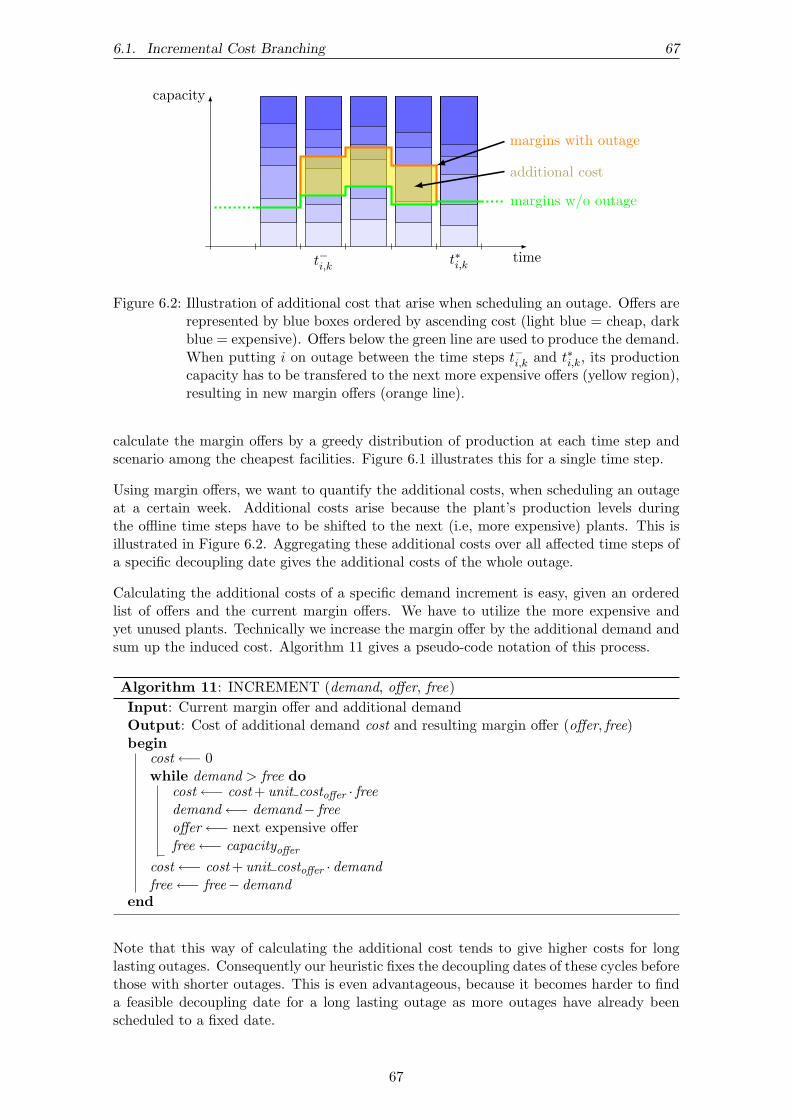
6.1. Incremental Cost Branching 67

capacity

timet−i,k t∗i,k

margins with outage

additional cost

margins w/o outage

Figure 6.2: Illustration of additional cost that arise when scheduling an outage. Offers arerepresented by blue boxes ordered by ascending cost (light blue = cheap, darkblue = expensive). Offers below the green line are used to produce the demand.When putting i on outage between the time steps t−i,k and t∗i,k, its productioncapacity has to be transfered to the next more expensive offers (yellow region),resulting in new margin offers (orange line).

calculate the margin offers by a greedy distribution of production at each time step andscenario among the cheapest facilities. Figure 6.1 illustrates this for a single time step.

Using margin offers, we want to quantify the additional costs, when scheduling an outageat a certain week. Additional costs arise because the plant’s production levels duringthe offline time steps have to be shifted to the next (i.e, more expensive) plants. This isillustrated in Figure 6.2. Aggregating these additional costs over all affected time steps ofa specific decoupling date gives the additional costs of the whole outage.

Calculating the additional costs of a specific demand increment is easy, given an orderedlist of offers and the current margin offers. We have to utilize the more expensive andyet unused plants. Technically we increase the margin offer by the additional demand andsum up the induced cost. Algorithm 11 gives a pseudo-code notation of this process.

Algorithm 11: INCREMENT (demand, offer, free)Input: Current margin offer and additional demandOutput: Cost of additional demand cost and resulting margin offer (offer, free)begin

cost←− 0while demand > free do

cost←− cost + unit costoffer · freedemand←− demand− freeoffer←− next expensive offerfree←− capacityoffer

cost←− cost + unit costoffer · demandfree←− free− demand

end

Note that this way of calculating the additional cost tends to give higher costs for longlasting outages. Consequently our heuristic fixes the decoupling dates of these cycles beforethose with shorter outages. This is even advantageous, because it becomes harder to finda feasible decoupling date for a long lasting outage as more outages have already beenscheduled to a fixed date.

67

68 6. Optimization

6.1.2 Outage Date Selection

In this section we focus on the selection of a best date of decoupling for a single outage.Furthermore, we add a cost value to this date, making it comparable to other outages.

We perform Algorithm 11 for each potential offline time step and aggregate the results foreach decoupling date (i.e, all weeks from the interval [ha(i, k), ha(i, k)+DAi,k]). Hence, weget a set of tuples consisting of decoupling dates and the corresponding additional costs.

Among these dates we are interested in selecting dates, which incur low additional costs,with higher probability. Therefore, we choose the k-th best out of n decoupling dateswith probability P[k] := 0.5k. The worst date is chosen with the residual probabilityP[n] := 1−

∑n−1k=1 P[k] = 0.5n−1.

To choose the cost of a selected decoupling date, we will try four measures. Rememberthat outages, which are more likely to produce higher additional cost, should get a highcost value assigned now. As the cost of the outage represents the set of possible dates, wecalculate it independently of the chosen decoupling date. The proposed measures are:

MAX: The most expensive decoupling date. Note that this measure does not care if alldecoupling date options are equally bad.

MED: The median of all available decoupling dates’ costs. This measure is resistantagainst outliers, but requires the most computational effort.

RANGE: The cost difference between the cheapest and most expensive decoupling date.

REGRET: The difference between the average and minimum costs. This measure providesa good estimation of the proportion of cheap decoupling dates.

6.1.3 Outage Selection

In the previous section we set up the choice of a best decoupling date for each outageand an associated cost value. We now have to choose one of these outages for branching.Since our primary goal is to save cost, we have to choose the outage with the highestcost here. Remember that additional costs are monotonically increasing while we schedulemore outages, hence an outage with already high costs matters most. Again, we order alloutages by their cost values and choose the more expensive outages with higher probability.Technically, we reuse the distribution function presented in Section 6.1.2.

6.1.4 Committing a Choice

Until now, we showed how to choose a probably good outage and one of its decouplingdates for a branching step. In this section we illustrate how the search space is splittedand changed when committing a choice.

A choice splits the search space into two branches. In the first we assign the chosendecoupling date to the specific outage, while we exclude this date from the domain ofdec∗i,k in the second branch (see Figure 6.3). Technically this is done by adding furtherconstraints (e.g., dec∗i,k = x) to the copied search space, when the commit procedure is runfor a specific alternative.

After adapting our model, we need to update the internal state of the margin offers inboth branches. In the first branch, where we assigned the decoupling date, we executeAlgorithm 11 for all time steps of the scheduled outage, increment the demand by the nowshut down production capacity and adjust the margin offers accordingly. In the secondbranch we do not change the margin offers, as there was no outage actively scheduled.Note that we will miss outages, which become assigned by constraint propagation.

68

6.1. Incremental Cost Branching 69

dec∗i,k ∈ {. . .}

dec∗i,k = x dec∗i,k 6= x

0 1

Figure 6.3: Branching alternatives by adding constraints. While we assign the chosenoutage date x in the left branch, we exclude it from the search space of rightbranch.


A00 0.05% >1000 0%A01 0.12% >1000 1%A02 0.19% >1000 11%A03 0.37% >1000 58%A04 0.62% 315 4%A05 1.19% 177 47%

B06 7.36% 47 24%B07 8.50% 32 9%B08 4 674.42% 25 0%B09 4 011.19% 21 0%B10 6.17% 10 2%

X11 5.72% 38 5%X12 3.88% 40 0%X13 9.73% 8 35%X14 9.67% 8 0%X15 2.84% 15 0%

Table 6.1: Incremental Cost Branching: We show the best achieved score (cf. Section 7.2)for all instances. Iterations lists the number of restarts, failure rate the propor-tion of iterations without a result. New best results are in bold font.

6.1.5 Evaluation

In this section we evaluate our results obtained by using incremental cost branching in-stead of the previously presented branching techniques. We start with the analysis of theproposed cost measures. In Figure 6.4 we show our experimental results on the A in-stances. Obviously, none of the measures has outstanding performance when compared tothe others. Accordingly, we assume that of order of the variable assignments (which is theeffect of the cost measures) has much less influence on the quality of an outage schedulethan the choice of a good decoupling date. From this point of view we might be able toreduce the complexity of the choice of the next outage to assign and still get results of asimilar quality.

The best results obtained for all instances by using incremental cost branching are shownin Table 6.1. The results are generally better than those presented in Section 5.3, butsuffer the same problems as random branching with the less-constrained instances B08and B09. Having a look into a concrete solution of B08 (see Figure 7.1), this can clearlybe attributed to our decision to postpone all optional outages.

The calculation of additional costs requires considerable effort, i.e., the number of roundsthat can be performed in the given time drops by a factor of around 5 when compared to

69

70 6. Optimization

Instance A01 Instance A02

0.10

0.15

0.20

0.30

0.40

max

med

rang

e

regr

et

scor

e in

%

0.2

0.3

0.4

0.5

max

med

rang

e

regr

et

scor

e in

%

Instance A03 Instance A04

0.4

0.5

0.6

0.7

max

med

rang

e

regr

et

scor

e in

%

0.6

0.7

0.8

0.9

1.0

max

med

rang

e

regr

et

scor

e in

%

Instance A05

12

5

max

med

rang

e

regr

et

scor

e in

%

Figure 6.4: Quality of cost measures: We compare the results obtained by the 4 proposedcost measures: Maximum, Median, Range and Regret. The plots show thedistribution of the obtained scores from 100 runs. The centered ticks at eachmeasure mark single results. Thick horizontal lines mark the mean achievedby each strategy. We omit the dummy-instance A00.

70

6.2. Decremental Cost Branching 71

048

048

time

production

40,000

60,000

80,000 capacity

demand

#outages RB

#outages ICB

Figure 6.5: Histograms of the best outage schedules found by random branching (RB)and incremental cost branching (ICB), compared to the capacity of all powerplants and the demand. We see that ICB schedules outages towards times oflow demand. The data are taken from scenario 0 of instance A05.

random branching. Furthermore, this branching technique results in less failures than purerandom branching. We guess this is caused by the fact that several outages which mightbe performed in an expensive region are assigned by the branching shortly after another.This results in earlier detection of infeasible states, because the majority of constraints –the spacing constraints – apply to outages which are scheduled within a short date range.Remember the sweep branching (SB, cf. Section 5.1.4.3) that assigned outages to theirearliest possible date in ascending order, i.e., it also schedules outages with similar rangesof their potential decoupling dates shortly after another. As SB also shows the smallestfailure rate among our basic branchings, we will combine SB and ICB in Section 6.3.

Finally, we analyze why this branching performs better. All previously presented branch-ings select outage dates without considering anything else than the variable’s domain.Therefore, these dates become somewhat equally distributed. Contrary, ICB considersmargin offers when selecting a date, which tend to have higher values when there is littleunused production capacity. In Figure 6.5 one can clearly see how ICB scheduled theoutages towards times with low demand and thus high unused capacity.

6.2 Decremental Cost Branching

Similar to incremental cost branching, we developed decremental cost branching, whichworks in opposite direction. In the beginning, we assume each Type-2 power plant isnot available for production during all time steps where it might be offline, i.e., betweenmin(dec∗i,k) and max(dec∗i,k)+DAi,k. We set up the margin offers accordingly, i.e., they arehigher than in a final solution. Branching again limits the domains of the dec∗i,k variables,thereby reducing the number of time steps a Type-2 power plant is not available. For allnewly available time steps we decrement the margin offers by the production capacity ofthe plant. In each branching step, we choose the outage that reduces the margin offers themost.

In our first experiments this branching did not perform as well as the incremental costbranching and was therefore dismissed.

71

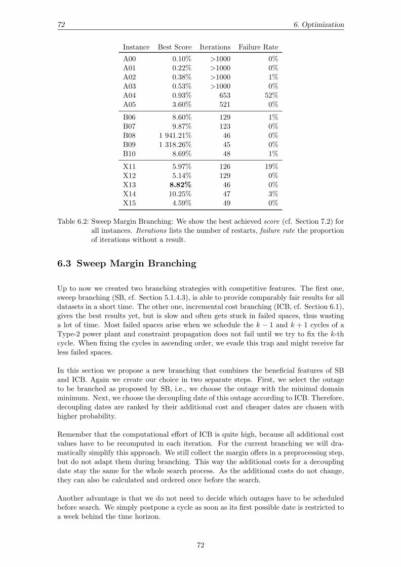
72 6. Optimization


A00 0.10% >1000 0%A01 0.22% >1000 0%A02 0.38% >1000 1%A03 0.53% >1000 0%A04 0.93% 653 52%A05 3.60% 521 0%

B06 8.60% 129 1%B07 9.87% 123 0%B08 1 941.21% 46 0%B09 1 318.26% 45 0%B10 8.69% 48 1%

X11 5.97% 126 19%X12 5.14% 129 0%X13 8.82% 46 0%X14 10.25% 47 3%X15 4.59% 49 0%

Table 6.2: Sweep Margin Branching: We show the best achieved score (cf. Section 7.2) forall instances. Iterations lists the number of restarts, failure rate the proportionof iterations without a result.

6.3 Sweep Margin Branching

Up to now we created two branching strategies with competitive features. The first one,sweep branching (SB, cf. Section 5.1.4.3), is able to provide comparably fair results for alldatasets in a short time. The other one, incremental cost branching (ICB, cf. Section 6.1),gives the best results yet, but is slow and often gets stuck in failed spaces, thus wastinga lot of time. Most failed spaces arise when we schedule the k − 1 and k + 1 cycles of aType-2 power plant and constraint propagation does not fail until we try to fix the k-thcycle. When fixing the cycles in ascending order, we evade this trap and might receive farless failed spaces.

In this section we propose a new branching that combines the beneficial features of SBand ICB. Again we create our choice in two separate steps. First, we select the outageto be branched as proposed by SB, i.e., we choose the outage with the minimal domainminimum. Next, we choose the decoupling date of this outage according to ICB. Therefore,decoupling dates are ranked by their additional cost and cheaper dates are chosen withhigher probability.

Remember that the computational effort of ICB is quite high, because all additional costvalues have to be recomputed in each iteration. For the current branching we will dra-matically simplify this approach. We still collect the margin offers in a preprocessing step,but do not adapt them during branching. This way the additional costs for a decouplingdate stay the same for the whole search process. As the additional costs do not change,they can also be calculated and ordered once before the search.

Another advantage is that we do not need to decide which outages have to be scheduledbefore search. We simply postpone a cycle as soon as its first possible date is restricted toa week behind the time horizon.

72

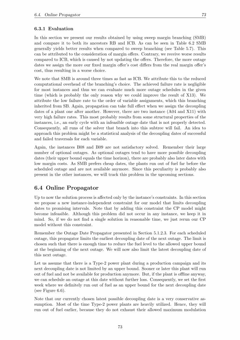
6.4. Online Propagator 73

6.3.1 Evaluation

In this section we present our results obtained by using sweep margin branching (SMB)and compare it to both its ancestors RB and ICB. As can be seen in Table 6.2 SMBgenerally yields better results when compared to sweep branching (see Table 5.7). Thiscan be attributed to the consideration of margin offers. Contrary, we receive worse resultscompared to ICB, which is caused by not updating the offers. Therefore, the more outagedates we assign the more our fixed margin offer’s cost differs from the real margin offer’scost, thus resulting in a worse choice.

We note that SMB is around three times as fast as ICB. We attribute this to the reducedcomputational overhead of the branching’s choice. The achieved failure rate is negligiblefor most instances and thus we can evaluate much more outage schedules in the giventime (which is probably the only reason why we could improve the result of X13). Weattribute the low failure rate to the order of variable assignments, which this branchinginherited from SB. Again, propagation can take full effect when we assign the decouplingdates of a plant one after another. However, there are two instance (A04 and X11) withvery high failure rates. This most probably results from some structural properties of theinstances, i.e., an early cycle with an infeasible outage date that is not properly detected.Consequently, all runs of the solver that branch into this subtree will fail. An idea toapproach this problem might be a statistical analysis of the decoupling dates of successfuland failed traversals for each variable.

Again, the instances B08 and B09 are not satisfactory solved. Remember their largenumber of optional outages. As optional outages tend to have more possible decouplingdates (their upper bound equals the time horizon), there are probably also later dates withlow margin costs. As SMB prefers cheap dates, the plants run out of fuel far before thescheduled outage and are not available anymore. Since this peculiarity is probably alsopresent in the other instances, we will track this problem in the upcoming sections.

6.4 Online Propagator

Up to now the solution process is affected only by the instance’s constraints. In this sectionwe propose a new instance-independent constraint for our model that limits decouplingdates to promising intervals. Note that by adding this constraint the CP model mightbecome infeasible. Although this problem did not occur in any instance, we keep it inmind. So, if we do not find a single solution in reasonable time, we just rerun our CPmodel without this constraint.

Remember the Outage Date Propagator presented in Section 5.1.2.3. For each scheduledoutage, this propagator limits the earliest decoupling date of the next outage. The limit ischosen such that there is enough time to reduce the fuel level to the allowed upper boundat the beginning of the next outage. We will now also limit the latest decoupling date ofthis next outage.

Let us assume that there is a Type-2 power plant during a production campaign and itsnext decoupling date is not limited by an upper bound. Sooner or later this plant will runout of fuel and not be available for production anymore. But, if the plant is offline anyway,we can schedule an outage at this date without further loss. Consequently, we set the firstweek where we definitely run out of fuel as an upper bound for the next decoupling date(see Figure 6.6).

Note that our currently chosen latest possible decoupling date is a very conservative as-sumption. Most of the time Type-2 power plants are heavily utilized. Hence, they willrun out of fuel earlier, because they do not exhaust their allowed maximum modulation

73

74 6. Optimization

fuel


post i,k

λ ·MMAXi,k

Figure 6.6: Reasoning by the Online Propagator: The latest possible decoupling date ofthe upcoming outage is limited to the week where the plant runs definitely outof fuel.

Instance A03 Instance B08

0.30

0.35

0.40

0.45

0.50

0 0.25 0.5 0.75 1

scor

e in

%

34

56

7

0 0.25 0.5 0.75 1

scor

e

Figure 6.7: Online Propagator: We compare the results obtained for different values ofλ ∈ {0, 0.25, 0.5, 0.75, 1}. The plots show the distribution of the obtainedscores (cf. Section 7.2) from around 15 runs per λ.

MMAXi,k completely. Therefore, we add a parameter λ ∈ [0, 1] to this constraint whichrepresents the exhausted proportion of MMAXi,k. In our experiments we will evaluatedifferent values for λ.

To determine the latest decoupling date, i.e., max(dec∗i,k+1), we perform a fuel level forwardpropagation (cf. Section 5.1.2.2). As the maximum production of a plant is achieved witha post-refueling fuel level of max(post i,k), we choose max(post i,k) + λ ·MMAXi,k as theinitial fuel level of the production campaign and perform maximum production, whichstarts at the latest possible coupling date max(dec∗i,k)+DAi,k. We set the first week whereproduction is ceased (see CT 6) as the upper bound of dec∗i,k+1.

We notice that there is one special case, where the current setup will result in failedspaces. This happens if the plant runs definitely out of fuel before the earliest possiblenext decoupling date. So, in this case we do not commit the infeasible upper bound butassign dec∗i,k+1 to its domain minimum.

6.4.1 Evaluation

In this section we discuss the results obtained after adding the Online Propagator to ourmodel. First we analyze the impact of λ. In Figure 6.7 we picked two sample instances

74

6.5. Residual Fuel Penalty 75


A00 0.05% >1000 0%A01 0.17% >1000 0%A02 0.28% >1000 0%A03 0.33% >1000 0%A04 0.72% 606 48%A05 0.63% 529 0%

B06 5.92% 123 2%B07 4.34% 119 0%B08 6.60% 47 0%B09 6.63% 45 3%B10 5.51% 48 2%

X11 4.94% 73 75%X12 3.76% 126 1%X13 5.35% 47 0%X14 5.37% 45 3%X15 2.85% 47 0%

Table 6.3: Online Propagator: We show the best achieved score for all instances. Iterationslists the number of restarts, failure rate the proportion of iterations without aresults. New best results are in bold font.

and evaluate their performance for varying proportions of modulation. We identify a cleartrend: less modulation yields better results. There are probably two reasons for this effect.Firstly, Type-2 power plants are fully utilized most of the time and thus consume theirfuel as fast as possibe. Secondly, the chosen fuel level before production max(post i,k) is anoverestimation. This seems plausible because the upper bound of post i,k assumes minimumproduction in the previous cycles, which is probably not the case.

In the following experiments we will always assume λ = 0.

Before, let us have a look on the results obtained after adding the propagator (see Ta-ble 6.3). First of all, we note that we improve the results of B08 and B09 up to a similarquality as our other solutions. Additionally, we can considerably improve the results ofmost other instances. The computational effort is nearly unchanged. So, although thenew constraint requires additional effort for propagation, this can be compensated by thesmaller search space.

6.5 Residual Fuel Penalty

Choosing outage dates based on their additional cost yields our best results yet. This iswhy we further analyze this strategy. Looking at the refueling formula CT 10 we realizethat we do not consider fuel levels before refueling as a factor of additional cost. But, thehigher this fuel level is, the more fuel is lost in the next refueling operation.

In the following we will analyze the influence of the fuel level before refueling to theadditional cost and increase this cost by an appropriate penalty. First, we set up a lowerbound of residual fuel (see Figure 6.8). We choose the minimum initial fuel level beforeproduction and perform maximum production, thus determining the minimum residualfuel level for each week of the domain of dec∗i,k+1.

We now analyze the consequences on the objective function caused by different fuel levelsbefore refueling. Let us assume two different fuel levels f1 = 0 and f2 = x(i, s, t−i,k) before

75

76 6. Optimization

fuel


post i,k

minimumresidual

fuel

Figure 6.8: For each possible decoupling date of dec∗i,k+1 we determine the minimum resid-ual fuel level.

refueling. After reloading the same amount of fuel, the difference between both fuel levelsreduced by x(i, s, t−i,k)/Qi,k (see CT 10). We call this difference the loss of fuel. Accordingto the objective function each unit of fuel is worth Ci,k. Hence, we add the followingpenalty to the additional cost of each week with a residual fuel amount of f :

penalty(f) :=Ci,k

Qi,k

· f

After adding the penalty to the additional cost and resorting the decoupling dates, theused branching technique proceeds as normal. Note that this penalty calculation is onlypractical for sweep margin branching, because there the penalties have to be calculatedonly for the outage chosen for branching. With incremental cost branching we would haveto calculate the penalties for all outages because the outage to branch is selected afterevaluating all decoupling dates.

6.5.1 Evaluation

In this section we present the results obtained after adding residual fuel penalties to thechoice of sweep margin branching (see Table 6.5). There is no significant impact on thefailure rate because the penalty just modifies the probabilities of the decoupling datesand does not further limit the search space. Besides, this technique hardly influences therunning time because the calculation is run only once at each branching step.

We can improve 4 of 16 solutions, but improvements are rather marginal. Contrary, thesolution quality of all other instances becomes worse. We assume that the impact of therealized outage schedules on the objective function is much stronger than the impact ofthe residual fuel levels. Accordingly, we should not consider the amount residual fuel inthe outage scheduling phase, but optimize the fuel levels afterwards. In the following, wewill not make further use of the residual fuel penalty.

6.6 Tuning Fuel Levels

Remember our basic refueling strategy (presented in Section 5.2.3) to always choose themaximum possible refueling amount. This is fast to compute, but not desirable for severalreasons. First, if the plant is operating at its maximum allowed fuel level, its productionlevel is imposed in order to stay below the maximum allowed fuel level at the end of theproduction campaign (cf. Section 5.2.2). So, the plant might have to produce althoughit is not among the cheapest plants. Second, reloading more fuel is expensive and as we

76

6.6. Tuning Fuel Levels 77


A00 0.05% >1000 0%A01 0.19% >1000 0%A02 0.28% >1000 1%A03 0.34% >1000 0%A04 0.76% 640 41%A05 0.91% 585 0%

B06 5.75% 125 0%B07 4.53% 122 0%B08 5.35% 47 0%B09 6.53% 44 2%B10 5.73% 48 2%

X11 5.34% 55 60%X12 4.05% 126 0%X13 5.10% 45 0%X14 6.43% 47 0%X15 2.98% 49 0%

Table 6.4: Residual Fuel Penalty: We show the best achieved score (cf. Section 7.2) for allinstances. Iterations lists the number of restarts, failure rate the proportion ofiterations without a results.

reload more fuel, we probably get a higher fuel level at the end of the production campaign,thus resulting in a higher penalty for residual fuel (see CT 10 and Section 6.5). On theother hand, reloading too little amounts of fuel results in less production, and hence alsohigher cost.

To determine a good refueling amount, we set up a model to forecast the profit induced bya certain refueling amount. We will estimate this profit from the initial cost of refueling,the production amounts and a penalty for the residual fuel level. Note that the cost ofthe initial and residual fuel levels can be easily determined. The key idea to transferproduction amounts into revenue is to run our production assignment phase twice. In thefirst run, we store the margin cost realized for each time step. We will use these cost inthe second run as the price of each produced unit of energy.

Algorithm 12: PROFIT (s, i, k, fuel level f , refueling r, margins c)Output: Estimated profit of the cycle when refueling rbegin

profit← −r · Ci,k

f ← fuel level, when refueling rfor time step t← t∗i,k to t+i,k do

prod← production with respect to the fuel level, modulation, unit cost, ...profit← profit+ prod · ct

if next cycle is scheduled thenprofit← profit− Ci,k+1

Qi,k+1· f

elseprofit← profit+ f · Ci,T

return profitend

77

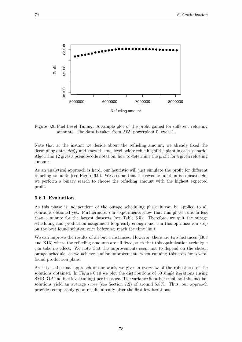
78 6. Optimization

● ● ● ● ● ● ● ● ● ● ● ● ● ● ● ● ● ● ● ● ● ● ● ● ● ● ● ● ● ● ●

5000000 6000000 7000000 8000000

0e+

004e

+08

8e+

08

Refueling amount

Pro

fit

Figure 6.9: Fuel Level Tuning: A sample plot of the profit gained for different refuelingamounts. The data is taken from A05, powerplant 0, cycle 1.

Note that at the instant we decide about the refueling amount, we already fixed thedecoupling dates dec∗i,k and know the fuel level before refueling of the plant in each scenario.Algorithm 12 gives a pseudo-code notation, how to determine the profit for a given refuelingamount.

As an analytical approach is hard, our heuristic will just simulate the profit for differentrefueling amounts (see Figure 6.9). We assume that the revenue function is concave. So,we perform a binary search to choose the refueling amount with the highest expectedprofit.

6.6.1 Evaluation

As this phase is independent of the outage scheduling phase it can be applied to allsolutions obtained yet. Furthermore, our experiments show that this phase runs in lessthan a minute for the largest datasets (see Table 6.5). Therefore, we quit the outagescheduling and production assignment loop early enough and run this optimization stepon the best found solution once before we reach the time limit.

We can improve the results of all but 4 instances. However, there are two instances (B08and X13) where the refueling amounts are all fixed, such that this optimization techniquecan take no effect. We note that the improvements seem not to depend on the chosenoutage schedule, as we achieve similar improvements when running this step for severalfound production plans.

As this is the final approach of our work, we give an overview of the robustness of thesolutions obtained. In Figure 6.10 we plot the distributions of 50 single iterations (usingSMB, OP and fuel level tuning) per instance. The variance is rather small and the mediansolutions yield an average score (see Section 7.2) of around 5.8%. Thus, our approachprovides comparably good results already after the first few iterations.

78

6.6. Tuning Fuel Levels 79

2 4 6 8 10

X15

X14

X13

X12

X11

B10

B09

B08

B07

B06

score in %

Figure 6.10: Robustness of our solution: We show the scores (cf. Section 7.2) of 50 it-erations on the B and X instances. Ticks mark single solutions. The thickvertical lines mark the median solution of each instance. Note that the av-erage expected score (dotted line) after one iteration of each instance is lessthan 6%.

79

80 6. Optimization

Instance Best Score Running Time [sec] Variability Improvement

A00 0.05% 1 28% 0.00%A01 0.07% 1 20% -0.03%A02 0.12% 2 21% -0.04%A03 0.22% 2 32% -0.10%A04 0.46% 5 24% -0.14%A05 0.55% 5 14% -0.07%

B06 5.37% 17 21% -0.13%B07 4.14% 16 39% -0.06%B08 6.60% 44 0% 0.00%B09 6.63% 43 22% 0.00%B10 4.91% 42 38% -0.52%

X11 4.55% 18 21% -0.30%X12 3.33% 16 38% -0.34%X13 5.35% 43 0% 0.00%X14 4.92% 45 22% -0.12%X15 2.40% 44 38% -0.37%

Table 6.5: Fuel Level Tuning: Score (cf. Section 7.2) presents the best solutions obtained.Column variability lists the average distance between the maximum and mini-mum allowed refueling amounts (RMAXi,k and RMINi,k) in the instance. Theother columns show the average running time of the extra auction round, andthe average improvement when applying this technique to results obtained with-out fuel level tuning.

80

7. Evaluation

We implemented the algorithms and methods which we describe in this thesis in C++and evaluated their performance by using the instances provided by the ROADEF/EUROChallenge 2010. In this chapter we introduce the general experimental setup and give anoverview of our experiments. As detailed evaluation is presented along with the develop-ment of our solution, we reference to the corresponding sections.

This chapter is organized as follows: First, we specify our implementation and testingenvironment in Section 7.1. Afterwards, in Section 7.2 we give an overview of the instancesthat have been used for evaluation and highlight their features. Section 7.3 summarizesthe results obtained by our presented methods and optimization steps. We conclude withthe best solutions found by our approach in Section 7.4.

7.1 Implementation and Testing Environment

We implemented of our solution in C++ and utilize two external libraries. First, forthe solution of the outage scheduling phase (cf. Section 5.1) we extend the constraintprogramming toolkit Gecode 3.3.2 [Gec10]. A detailed introduction into Gecode is givenin Section 2.1.1. To solve the Minimum-Cost Flow Problem of the network-based lowerbound (cf. Section 4.3) we use the implementation of the Cost-Scaling Algorithm from theLemon Graph Library 1.2 [Lem10].

The mentioned libraries and our code have been compiled with GCC 4.3, using optimiza-tion level 3. Our presented experiments have been performed on one core of a 2x dual-coreAMD Opteron Processor 2218 clocked at 2.6 GHz, equipped with 1 MB L2 Cache per coreand 32 GB RAM. We notice that this setup is slightly less powerful than the referencesetup used in the competition (2x quad-core Intel Xeon 5420 at 2.5 GHz, 12 MB L2 Cache,8 GB RAM). Our solutions are run as a single thread and do not consume more than 8GB of memory per process.

7.2 Provided Datasets

Three datasets (A, B and X) have been provided by the ROADEF/EURO Challenge 2010.While the first two sets have always been available to us, the X set – which was meant forfinal evaluation of the challenge – was published two weeks before we finished this work.The A set contains 6 small instances, while the B and X sets comprise 5 big instances each.

81

82 7. Evaluation

Instance # Power Plants Scenarios Weeks Timesteps # ConstraintsType-1 Type-2 13 14–18 19 20 21

A00 1 2 2 89 623 4 1 0 0 0A01 11 10 10 250 1750 46 11 1 1 1A02 21 18 20 250 1750 84 17 1 1 1A03 21 18 20 250 1750 80 18 1 1 1A04 31 30 30 250 1750 122 23 1 1 1A05 31 28 30 250 1750 120 22 1 1 3

B06 25 50 50 277 5817 222 77 1 50 5B07 27 48 50 265 5565 192 70 1 50 5B08 19 56 121 277 5817 114 86 1 50 5B09 19 56 121 277 5817 114 86 1 50 5B10 19 56 121 265 5565 235 86 1 50 5

X11 25 50 50 277 5817 239 77 1 50 5X12 27 48 50 263 5523 207 70 1 50 5X13 19 56 121 277 5817 260 86 1 50 5X14 19 56 121 277 5817 256 86 1 50 5X15 19 56 121 263 5523 245 86 1 50 5

Table 7.1: Overview of the instances provided by the ROADEF/EURO Challenge 2010.

Their key figures are shown in Table 7.2. Note that the ratio between Type-1 and Type-2power plants is nearly 1 : 1 in set A, while the sets B and X comprise 2-3 times more Type-2 power plants than Type-1 power plants. As most of our constraint types are related toType-2 power plants the B and X instances require much more effort. Additionally, someinstances contain more than 120 different demand scenarios, therefore resulting in morethan 50 million decision variables in a single instance.

All instances – except the dummy-instance A00 – contain 6 cycles for each Type-2 powerplant. From the original problem description we derive that a time step’s duration in realtime is between 8 and 24 hours. The demand scenarios show similar characteristics andseem realistic (e.g., clear seasonal oscillation). Besides, there is no artificial variability,as would anyway be unrealistic from a power network control point of view. InstancesB08 and B09 are a bit special as they contain less outage date range constraints CT 13,which dramatically increases the search space, making it harder to find the best solution.Furthermore, in B08 and X13 all refueling amounts are fixed (i.e., RMINi,k = RMAXi,k).

All instances contain one Type-1 power plant that is able to cover the complete demand– at extremely high cost though. This plant can be seen as a backup plant to keep theproblems feasible. As it is never desirable to utilize this plant, we will omit it in all plotsand figures.

To make solution qualities comparable, the ROADEF/EURO Challenge 2010 defines aso called score on each result, which corresponds to the result’s deviation from the bestknown solution in percent. Assume that R is our solution and R′ the best known solutionso far, then the score is calculated as:

score(R) :=cost(R)cost(R′)

− 1

where cost returns the result’s value of the objective function. In the competition teamsare ranked by their average score for all B and X instances. Each unsolved instance givesa penalty of two times the score of the worst submitted solution.

82

7.3. Evolution of Results 83

Note that the objective function measures solutions in abstract monetary units. Since theseare huge numbers and rather unhandy, we will always use the score (given in percent) whencomparing our results.

7.3 Evolution of Results

In this section we show how our best solutions evolve while we add the presented opti-mization techniques (see Table 7.2). Remember that we rerun our solver until we reachthe time limit for the given instance. In each iteration we first search for a valid outageschedule. Afterwards, we perform a production assignment for the found schedule andupdate our best solution if necessary. If we do not find a valid outage schedule within acertain time, we also proceed to the next iteration.

Our basic solution from Chapter 5 performs one iteration with sweep branching (SB) toget a first reasonable result. Afterwards random branching (RB) is performed. The basicsolution provides fair results with an average score of 11.21%. Difficulties arise in theinstances B08 and B09 because they comprise a lot of optional cycles, which we do notschedule efficiently. In Section 6.1 we replace RB by incremental cost branching (ICB) andcan improve most results because the consideration of additional cost for the respectivedecoupling dates yields more promising outage schedules. Since ICB is rather slow, wecombine it with SB in Section 6.3. The resulting sweep margin branching (SMB) obtainsbetter results than those of SB and runs much faster than ICB. However, its results arenot as good as those of ICB. The remaining optimization techniques work all with SMB.In Section 6.4 we add the online propagator (ON) to our model, which limits the domainsof outage dates to promising values, thus dramatically reducing the search space. We areable to find comparable good results for the instances B08 and B09 for the first time andcan improve most other best solutions, resulting in an average score of 5.13%. In Figure 7.1we present some charts of our best production plans achieved by ICB, SMB and OP. Onecan see that the available production capacity of the Type-2 power plants sinks over timebecause we postpone all optional schedules, while SMB utilizes these cycles and keepsthe production capacity at a fair level. With ON the plan becomes more regular and theavailable Type-2 power plant production capacity can be increased again.

Afterwards, in Section 6.5 we modify the search order of SMB by introducing penaltiesfor undesirable residual fuel levels of the production campaigns. Although this techniquecan improve the results of 4 instances the overall solution quality becomes worse. Wedismiss this technique and add a deterministic postprocessing of the best found solutions inSection 6.6. It repeats the production assignment phase and utilizes an improved refuelingstrategy that is based on knowledge from the first run of the production assignment phase.This technique again improves most of our results.

7.4 Best Solutions

In this section we present the best solutions found by our approach. First of all, wenote that our obtained solution quality for A instances is much better than for B and Xinstances. This probably originates from some nice properties of the A instances: theycomprise less spacing constraints and outages to schedule and thus the search spaces aresmaller.

Among the B and X instances we achieve good results with a robust deviation from thebest known solution (see Figure 6.10). Unfortunately, we have not been able to improvethe best known results for the provided instances. Remember that only the B and Xinstances are considered for the ranking of the ROADEF/EURO Challenge 2010. Acrossthese instances we gained an average score of 4.66% which corresponds to the second bestrating in the competition.

83

84 7. Evaluation

SectionsMethod 5 6.1 6.3 6.4 6.5 6.6

1× SBn× RBn× ICBn× SMBONPENFUEL

Instance 5 6.1 6.3 6.4 6.5 6.6

A00 0.12% 0.05% 0.10% 0.05% 0.05% 0.05%A01 0.37% 0.12% 0.22% 0.17% 0.19% 0.07%A02 0.61% 0.19% 0.38% 0.28% 0.28% 0.12%A03 0.71% 0.37% 0.53% 0.33% 0.34% 0.22%A04 1.83% 0.62% 0.93% 0.72% 0.76% 0.46%A05 2.26% 1.19% 3.60% 0.63% 0.91% 0.55%

B06 8.16% 7.36% 8.60% 5.92% 5.75% 5.37%B07 9.39% 8.50% 9.87% 4.34% 4.53% 4.14%B08 17.88% 17.88% 17.88% 6.60% 5.35% 6.60%B09 27.90% 27.90% 27.90% 6.63% 6.53% 6.63%B10 8.25% 6.17% 8.69% 5.51% 5.73% 4.91%

X11 6.54% 5.72% 5.97% 4.94% 5.34% 4.55%X12 6.04% 3.88% 5.14% 3.76% 4.05% 3.33%X13 10.29% 9.73% 8.82% 5.35% 5.10% 5.35%X14 12.00% 9.67% 10.25% 5.37% 6.43% 4,92%X15 5.61% 2.84% 4.59% 2.85% 2.98% 2.40%max(B +X) 27.90% 27.90% 27.90% 6.63% 6.53% 6.63%avg(B +X) 11.21% 9.97% 10.77% 5.13% 5.18% 4.82%

Table 7.2: Evolution of results: The upper table shows the utilized methods of each section.We show sweep branching(SB, cf. 5.1.4.3), random branching(RB, cf. 5.1.4.2),incremental cost branching(ICB, cf. 6.1), sweep margin branching(SMB, cf. 6.3),the online propagator(ON, cf. 6.4), residual fuel penalty(PEN, cf. 6.5) and tun-ing fuel levels(FUEL, cf. 6.6). In the lower table we list the best scores obtainedin each section. Improvements to previous steps are in bold font.

84

7.4. Best Solutions 85

Figure 7.1: Sample Production Plans: We show three different solutions to instance B08aggregating all power plants. The upper solution was found by ICB, while bothother have been found by SMB. The lower solution was found after adding theonline propagator (OP) to our model. There are lines for the gross capacity ofall plants (blue), the demand (green), the gross capacity of all Type-2 powerplants (purple) and the minimum capacity of all plants (red). The light (dark)gray region marks the available production capacity of all Type-1 (Type-2)Power Plants. We clearly see that the plants run out of fuel and become un-available when using incremental cost branching, because all optional cycles arepostponed. While SMB performs better the online propagator again increasesthe available capacity.

85

86 7. Evaluation

Instance Best Known Solution Our Best Solution Score

A00 8 730 985 367 093 8 735 652 150 125 0.05%A01 169 538 386 903 169 661 789 155 0.07%A02 146 048 433 973 146 226 213 771 0.12%A03 154 429 888 940 154 775 064 397 0.22%A04 111 591 350 516 112 106 431 505 0.46%A05 125 822 236 385 126 509 328 020 0.55%

B06 83 424 716 217 87 901 956 744 5.37%B07 81 174 243 138 84 535 993 963 4.14%B08 81 926 206 073 86 308 981 283 5.35% *B09 81 750 858 197 87 092 422 958 6.53% *B10 77 767 024 999 81 587 212 103 4.91%

X11 79 116 772 289 82 718 992 355 4.55%X12 77 589 910 940 80 171 684 438 3.33%X13 76 449 207 715 80 345 858 956 5.10% *X14 76 172 998 633 79 921 258 048 4.92%X15 75 101 398 439 76 901 330 176 2.40%

Table 7.3: Best solutions: We compare the costs of the best known results to our bestachieved results. Note that the starred solutions (B08, B09, X13) have beenfound using the residual fuel penalty from Section 6.5. All other best solutionshave been found by tuning fuel levels instead (cf. Section 6.6).

86

8. Conclusion

In this thesis we solved the problem posed by the ROADEF/EURO Challenge 2010, whichcontained an industry scale power plant production planning problem in an uncertain andhighly constrained environment. The overall objective function was to reduce the totaloperating cost.

We developed two lower bounds for the problem. One is a fast greedy heuristic, the other isbased on a flow network and yields closer bounds at the cost of high computational effort.We decomposed the main problem into two stages: outage scheduling and productionassignment. For the first stage we formulated the given model as a constraint programand added further constraints which ensure the feasibility of the remaining productionassignment problem. In the second stage we utilized a greedy heuristic – developed fromour greedy lower bound – to assign production levels and refueling amounts for a givenoutage schedule.

We applied several optimization techniques to our basic solution. First, we improved thesearch for good outage schedules by randomization, identifying promising outage dates andchoosing them with a higher probability. We further analyzed the problem and developeda new constraint which removes undesirable outage schedules from the search space. Atlast we improved our production assignment stage by running it twice, utilizing knowledgefrom the first run throughout the second.

We implemented all the proposed methods and evaluated their performance on 16 instanceswhich have been provided by the French utility company EDF and are extracted from realworld data. For all experiments we kept as close as possible to the specifications of thecompetition.

Finally, we related this work to the results obtained by the participating teams of theROADEF/EURO Challenge 2010. Our approach is able to solve all proposed instances,which only 4 of 21 finalist teams did achieve. In our experiments we gained very competitiveresults with an average deviation from the best known results of less than 5%. Thiscorresponds to the second best score achieved in the competition.

87

88 8. Conclusion

88

List of Figures

2.1 Illustration of different branching techniques . . . . . . . . . . . . . . . . . . 92.2 Removal of minimum capacities . . . . . . . . . . . . . . . . . . . . . . . . . 11

3.1 Power plants vs. demand scenarios . . . . . . . . . . . . . . . . . . . . . . . 143.2 Illustration of a Type-1 power plant . . . . . . . . . . . . . . . . . . . . . . 143.3 Illustration of a Type-2 power plant . . . . . . . . . . . . . . . . . . . . . . 15

4.1 Sketch of the flow network lower bound . . . . . . . . . . . . . . . . . . . . 32

5.1 Conflicting variables of consecutive cycles. . . . . . . . . . . . . . . . . . . . 485.2 Illustration of imposed power profiles . . . . . . . . . . . . . . . . . . . . . . 495.3 Fuel level forward propagation . . . . . . . . . . . . . . . . . . . . . . . . . 515.4 Fuel level backward propagation . . . . . . . . . . . . . . . . . . . . . . . . 525.5 Outage date forward propagation . . . . . . . . . . . . . . . . . . . . . . . . 535.6 Outage date backward propagation . . . . . . . . . . . . . . . . . . . . . . . 535.7 Illustration of the overall solution process . . . . . . . . . . . . . . . . . . . 615.8 Comparison of early vs. late outages . . . . . . . . . . . . . . . . . . . . . . 63

6.1 Illustration of a marginal offer . . . . . . . . . . . . . . . . . . . . . . . . . . 666.2 Illustration of additional cost . . . . . . . . . . . . . . . . . . . . . . . . . . 676.3 Branching alternatives . . . . . . . . . . . . . . . . . . . . . . . . . . . . . . 696.4 Quality of ICB cost measures . . . . . . . . . . . . . . . . . . . . . . . . . . 706.5 Histogram comparison: random branching vs. incremental cost branching . 716.6 Illustration of reasoning by the Online Propagator . . . . . . . . . . . . . . 746.7 Quality of the Online Propagator with respect to λ . . . . . . . . . . . . . . 746.8 Illustration of residual fuel levels . . . . . . . . . . . . . . . . . . . . . . . . 766.9 An example of Fuel Level Tuning . . . . . . . . . . . . . . . . . . . . . . . . 786.10 Robustness of our approach . . . . . . . . . . . . . . . . . . . . . . . . . . . 79

7.1 Sample production plans from a real instance . . . . . . . . . . . . . . . . . 85

89

90 List of Figures

90

List of Tables

4.1 Results of the proposed lower bounds . . . . . . . . . . . . . . . . . . . . . . 42

5.1 Overview of the solution steps and considered constraints . . . . . . . . . . 445.2 Variables of a cycle . . . . . . . . . . . . . . . . . . . . . . . . . . . . . . . . 475.3 Parameters of fuel level forward propagation . . . . . . . . . . . . . . . . . . 515.4 Parameters of fuel level backward propagation . . . . . . . . . . . . . . . . 525.5 Results from smallest domain branching . . . . . . . . . . . . . . . . . . . . 625.6 Results from random branching . . . . . . . . . . . . . . . . . . . . . . . . . 625.7 Results from basic branching techniques . . . . . . . . . . . . . . . . . . . . 64

6.1 Results from the incremental cost branching . . . . . . . . . . . . . . . . . . 696.2 Results from sweep margin branching . . . . . . . . . . . . . . . . . . . . . 726.3 Results from the Online Propagator . . . . . . . . . . . . . . . . . . . . . . 756.4 Results from Residual Fuel Penalty . . . . . . . . . . . . . . . . . . . . . . . 776.5 Results from Fuel Level Tuning . . . . . . . . . . . . . . . . . . . . . . . . . 80

7.1 Overview of instances . . . . . . . . . . . . . . . . . . . . . . . . . . . . . . 827.2 Evolution of results . . . . . . . . . . . . . . . . . . . . . . . . . . . . . . . . 847.3 Best Solutions . . . . . . . . . . . . . . . . . . . . . . . . . . . . . . . . . . . 86

91

92 List of Tables

92

List of Algorithms

1 A greedy heuristic for demand distribution . . . . . . . . . . . . . . . . . . . 29

2 Assembly of the auction-based lower bound . . . . . . . . . . . . . . . . . . . 30

3 Upper bound calculation of previous fuel levels . . . . . . . . . . . . . . . . . 50

4 CP formulation of the limited resources CT 19 . . . . . . . . . . . . . . . . . 55

5 CP formulation of the maximum number of outages CT 20 . . . . . . . . . . 55

6 CP formulation of the maximum offline power capacity CT 21 . . . . . . . . 55

7 Precalculation of the maximum allowed fuel level per time step . . . . . . . . 58

8 Assembly of minimum offers of Type-2 power plants . . . . . . . . . . . . . 59

9 Assembly of maximum offers of Type-2 power plants . . . . . . . . . . . . . 60

10 Determination of the refueling amount . . . . . . . . . . . . . . . . . . . . . . 60

11 Calculation of additional cost using marginal offers . . . . . . . . . . . . . . . 67

12 Calculation of the profit induced by a given refueling amount . . . . . . . . . 77

93

94 List of Algorithms

94

Bibliography

[AMO93] R. K. Ahuja, T. L. Magnanti, and J. B. Orlin, Network Flows: Theory, Algo-rithms, and Applications. Prentice-Hall, Inc., 1993.

[BC02] N. Beldiceanu and M. Carlsson, “A New Multi-resource cumulatives Constraintwith Negative Heights,” in Proceedings of the 8th International Conference onPrinciples and Practice of Constraint Programming. Springer-Verlag, 2002,pp. 63–79.

[CLRS01] T. H. Cormen, C. E. Leiserson, R. L. Rivest, and C. Stein, Introduction toAlgorithms, 2nd ed. MIT Press, 2001.

[DR97] D. Dentcheva and W. Romisch, “Optimal Power Generation under Uncertaintyvia Stochastic Programming,” in Stochastic Programming Methods and Techni-cal Applications, Lecture Notes in Economics and Mathematical Systems 458,K. Marti and P. Kall, Eds. Springer-Verlag, 1997, pp. 22–56.

[FKL96] S. Feltenmark, K. C. Kiwiel, and P. Lindberg, “Solving Unit Commitment Prob-lems in Power Production Planning,” in Operations Research Proceedings 1996.Springer-Verlag, 1996, pp. 236–241.

[FMS08] W. K. Foong, H. R. Maier, and A. R. Simpson, “Power Plant MaintenanceScheduling Using Ant Colony Optimization: An Improved Formulation,” Engi-neering Optimization, vol. 40, pp. 309 – 329, 2008.

[Gec10] “GECODE - A Generic Constraint Development Environment,” http://www.gecode.org, 2010.

[GT90] A. V. Goldberg and R. E. Tarjan, “Finding Minimum-Cost Circulations bySuccessive Approximation,” Mathematics of Operations Research, vol. 15, no. 3,pp. 430–466, 1990.

[Kid09] S. Kidd, “Nuclear in France - What Did They Get Right?” NuclearEngineering International Magazine, 2009. [Online]. Available: http://www.neimagazine.com/story.asp?storyCode=2053355

[KPB06] M. O. I. Khemmoudj, M. Porcheron, and H. Bennaceur, “When ConstraintProgramming and Local Search Solve the Scheduling Problem of Electricite deFrance Nuclear Power Plant Outages,” in Principles and Practice of ConstraintProgramming, Lecture Notes in Computer Science 4204, 2006, pp. 271–283.

[Lem10] “LEMON Graph Library,” http://lemon.cs.elte.hu, 2010.

[LES07] K. Y. Lee and M. A. El-Sharkawi, Modern Heuristic Optimization Techniques:Theory and Applications to Power Plants. Wiley-Interscience, 2007.

[NKT00] J. M. Ngundam, F. Kenfack, and T. T. Tatietse, “Optimal Scheduling of Large-Scale Hydrothermal Power Systems Using the Lagrangian Relaxation Tech-nique,” International Journal of Electrical Power & Energy Systems, vol. 22,no. 4, pp. 237 – 245, 2000.

95

http://www.gecode.org

http://www.gecode.org

http://www.neimagazine.com/story.asp?storyCode=2053355

http://www.neimagazine.com/story.asp?storyCode=2053355

http://lemon.cs.elte.hu

96 Bibliography

[NW88] G. L. Nemhauser and L. A. Wolsey, Integer and Combinatorial Optimization.Wiley-Interscience, 1988.

[Pad04] N. Padhy, “Unit Commitment - A Bibliographical Survey,” Power Systems,IEEE Transactions on, vol. 19, no. 2, pp. 1196 – 1205, 2004.

[PGJ+] M. Pocheron, A. Gorge, O. Juan, T. Simovic, and G. Dereu, “ChallengeROADEF/EURO 2010: A Large-Scale Energy Management Problem withVaried Constraints.” [Online]. Available: http://challenge.roadef.org/2010/

[RBW06] F. Rossi, P. v. Beek, and T. Walsh, Handbook of Constraint Programming(Foundations of Artificial Intelligence). Elsevier Science Inc., 2006.

[SK98] S. Sen and D. P. Kothari, “Optimal Thermal Generating Unit Commitment: AReview,” International Journal of Electrical Power & Energy Systems, vol. 20,no. 7, pp. 443 – 451, 1998.

[SN91] T. Satoh and K. Nara, “Maintenance Scheduling by Using Simulated AnnealingMethod [for Power Plants],” Power Systems, IEEE Transactions on, vol. 6, pp.850 – 857, 1991.

[STL10] C. Schulte, G. Tack, and M. Z. Lagerkvist, “Modeling and Programming withGecode,” www.gecode.org/doc-latest/MPG.pdf, 2010, online handbook.

[Tac09] G. Tack,“Constraint Propagation – Models, Techniques, Implementation,”Doc-toral Dissertation, Saarland University, 2009.

[WW96] A. J. Wood and B. F. Wollenberg, Power Generation, Operation, and Control,2nd ed. Wiley-Interscience, 1996.

96

http://challenge.roadef.org/2010/

www.gecode.org/doc-latest/MPG.pdf

Documents

Solving a Large-Scale Energy Management Problem With ... · Reviewer: Prof. Dr. rer. nat. Dorothea Wagner Advisors: Dipl.-Math. Reinhard Bauer Dr.-Ing. Andreas Cardeneo Dipl.-Inform