Solvable Nonlinear Evolution PDEs in Multidimensional …emis.dsd.sztaki.hu/journals/SIGMA/2006/Paper088/sigma06-088.pdf · 2 F. Calogero and M. Sommacal which is rotation-invariant

Symmetry, Integrability and Geometry: Methods and Applications Vol. 2 (2006), Paper 088, 17 pages

Solvable Nonlinear Evolution PDEs

in Multidimensional Space?

Francesco CALOGERO † and Matteo SOMMACAL ‡§

† Dipartimento di Fisica, Universita di Roma “La Sapienza”,Istituto Nazionale di Fisica Nucleare, Sezione di Roma,P.le Aldo Moro 2, 00185 Rome, ItalyE-mail: [email protected], [email protected]

‡ Laboratoire J.-L. Lions, Universite Pierre et Marie Curie, Paris VI,175 Rue du Chevaleret, 75013 Paris, France (until October 30th, 2006)

§ Dipartimento di Matematica, Universita di Perugia,Via Vanvitelli 1, 06123 Perugia, Italy (from November 1st, 2006)E-mail: [email protected]

Received October 31, 2006; Published online December 08, 2006Original article is available at http://www.emis.de/journals/SIGMA/2006/Paper088/

Abstract. A class of solvable (systems of) nonlinear evolution PDEs in multidimensionalspace is discussed. We focus on a rotation-invariant system of PDEs of Schrodinger type andon a relativistically-invariant system of PDEs of Klein–Gordon type. Isochronous variantsof these evolution PDEs are also considered.

Key words: nonlinear evolution PDEs in multidimensions; solvable PDEs; NLS-like equa-tions; nonlinear Klein–Gordon-like equations; isochronicity

2000 Mathematics Subject Classification: 35G25; 35Q40; 37M05

This article is dedicated to the memory of Vadim Kuznetsov, with whom we spentseveral happy days during a Gathering of Scientists held at the Centro Internacionalde Ciencias in Cuernavaca, and as well when he visited us in Rome, and when wemet at several other meetings.

1 Introduction

Over a decade ago a class of C-integrable – i.e., solvable via a Change of variables – systemsof PDEs in multidimensional space were identified [2]. (A problem involving nonlinear PDEsis considered solvable if its solution can be obtained by performing algebraic operations – suchas finding the zeros of a given polynomial – and by solving linear PDEs; of course only seldomthese operations can be performed explicitly.) In the present paper – motivated by the scarcityof solvable models of nonlinear evolution PDEs in multidimensions hence by the interest of anysuch model – we study (a subclass of) these solvable PDEs in more detail than it was donehitherto. We focus mainly on the system of PDEs of Schrodinger type

iψn,t −∆ψn +W (~r)ψn = 2N∑

m=1,m 6=n

a+ bψnψm −(~∇ψn

)·(~∇ψm

)ψn − ψm

, (1.1)

?This paper is a contribution to the Vadim Kuznetsov Memorial Issue “Integrable Systems and Related Topics”.The full collection is available at http://www.emis.de/journals/SIGMA/kuznetsov.html

mailto:[email protected]



http://www.emis.de/journals/SIGMA/2006/Paper088/

http://www.emis.de/journals/SIGMA/kuznetsov.html

2 F. Calogero and M. Sommacal

which is rotation-invariant if W (~r) = W (r), and on the relativistically-invariant system of PDEsof Klein–Gordon type

ψn,tt −∆ψn +M2ψn = 2N∑

m=1,m 6=n

a+ bψnψm + ψn,tψm,t −(~∇ψn

)·(~∇ψm

)ψn − ψm

. (1.2)

Notation. Here and throughout N is an arbitrary positive integer (N ≥ 2); the index n,as well as other analogous indices (see below), range generally from 1 to N ; the dependentvariables ψn ≡ ψn (~r, t) are generally considered complex (although this is only mandatory forthe first, (1.1), of these two systems of PDEs); the space variable ~r is a (real) S-vector (withS arbitrary : for S = 3, ~r ≡ (x, y, z)), and r indicates its modulus, r2 = ~r · ~r; a dot sandwichedamong two S-vectors denotes the standard (rotation-invariant) scalar product (for instance,for S = 3, ~r · ~r = x2 + y2 + z2); the “potential” W (~r) is an arbitrary function of the spatialcoordinate ~r (we will often assume that it only depends on the modulus r of the S-vector ~r); theconstants a and b, as well as the “mass” parameter M, are arbitrary (they might also vanish); t isthe (real) time variable; subscripted independent variables always denote partial differentiations;~∇ respectively ∆ ≡ ~∇ · ~∇ are the gradient respectively the Laplace operator in S-dimensionalspace. Isochronous variants of these evolution PDEs are also considered.

In the following Section 2 we review tersely the general class of PDEs treatable in thismanner and the technique to solve them. In Sections 3 respectively 4 we treat in some detailthe PDEs (1.1) respectively (1.2), describing various properties of their solutions and reportingsome representative examples, and we exhibit their isochronous versions. In Section 5 we takeadvantage of the electronic format of this article to present a few animations displaying visuallythe time evolution of a few solutions of some of these solvable (systems of) nonlinear evolutionPDEs: in this article we restrict these presentations to very few cases, all with space dimensiona-lity less than three (we are of course aware that the three-dimensional case is probably the mostinteresting one – since we seem to live in a three-dimensional world – but the presentation ofanimations in a three-dimensional context is somewhat more tricky and we therefore postponethe display of such examples to future articles we hope to issue soon). In Section 6 we outlinefuture directions of research.

2 A class of solvable (systems of) PDEsin multidimensional space

In this section we review tersely the basic idea allowing to identify a class of solvable nonlinearevolution PDEs. The interested reader will find a more detailed treatment in the paper wherethis approach was introduced [1], and especially in [3] where this method is treated in con-siderable detail: see Section 2.3 of this book, and other references quoted there in Section 2.N.These treatments focussed however on ODEs rather than PDEs: the extension to PDEs is ratherstraightforward, although it took some time to realize its feasibility [2] (see also Exercise 2.3.4.2-5in [3]).

Let Ψ (ψ;~r, t) be a (time- and space-dependent) monic polynomial of degree N in the vari-able ψ, and denote by ψn (~r, t) its N zeros and by ϕm (~r, t) its N coefficients:

Ψ (ψ;~r, t) =N∏n=1

[ψ − ψn (~r, t)] , (2.1a)

Ψ (ψ;~r, t) = ψN +N∑m=1

ϕm (~r, t)ψN−m. (2.1b)

Solvable Nonlinear Evolution PDEs in Multidimensional Space 3

Assume then that the time evolution of the dependent variable Ψ – hence its dependence onthe time and space independent variables t and ~r, as well as its dependence on the independentvariable ψ – is characterized by a linear evolution PDE, which must of course be consistent withthe fact that Ψ is, for all time, a monic polynomial of degree N in ψ, see (2.1). The linearcharacter of this PDE entails that the time-evolution of the N coefficients ϕm (~r, t), see (2.1b),is as well linear, possibly explicitly solvable (see below). On the other hand the correspondingtime evolution of the N zeros ψn (~r, t) will be nonlinear, due to the nonlinear character of themapping relating the N zeros ψn (~r, t) to the N coefficients ϕm (~r, t) of the polynomial Ψ (ψ;~r, t),see (2.1). These (systems of) nonlinear evolution PDEs satisfied by the dependent variablesψn (~r, t) are those referred to in the title of this paper: they are indeed generally solvable bytaking advantage of the mapping, see (2.1), relating the N dependent variables ψn (~r, t) to theN functions ϕm (~r, t).

In particular it is easily seen (using, if need be, the formulas provided in Section 2.3 of [3]),that to the evolution PDE

iΨt −∆Ψ− V (~r) (ψΨψ −NΨ) + aΨψψ + b[ψ2Ψψψ −N (N − 1) Ψ

]= 0 (2.2)

satisfied by Ψ (ψ;~r, t) , there corresponds for the N zeros ψn (~r, t) , see (2.1a), just the systemof nonlinear evolution PDEs of Schrodinger type (1.1) with

W (~r) = V (~r)− 2 (N − 1) b, (2.3)

while the corresponding evolution of the N coefficients ϕm (~r, t), see (2.1b), is clearly given bythe system of linear evolution PDEs

iϕm,t −∆ϕm + [W (~r)− b (m+ 3)]mϕm= −a (N −m+ 2) (N −m+ 1)ϕm−2, m = 1, . . . , N (2.4)

with ϕ−1 = 0 and ϕ0 = 1 (see (2.1b)). Note that this system of linear PDEs is decoupled if theconstant a vanishes; as we shall see in the following section, it can also be replaced by a decoupledsystem if the constant a does not vanish, a 6= 0, but the potential W (~r) is constant, W (~r) = C,see Section 3.

Likewise to the evolution PDE

Ψtt −∆Ψ− µ2 [ψΨψ −NΨ] + aΨψψ + b[ψ2Ψψψ −N (N − 1) Ψ

]= 0, (2.5)

there corresponds for the N zeros ψn (~r, t) just the system of nonlinear evolution PDEs ofKlein–Gordon type (1.2) with

M2 = µ2 − 2 (N − 1) b,

while the corresponding evolution of the N coefficients ϕm (~r, t) is clearly given by the systemof linear evolution PDEs

ϕm,tt −∆ϕm +[M2 − b (m+ 3)

]mϕm

= −a (N −m+ 2) (N −m+ 1)ϕm−2, m = 1, . . . , N, (2.6)

again with ϕ−1 = 0 and ϕ0 = 1 (see (2.1b)): this system is decoupled if the constant a vanishes,and can be replaced by a decoupled system even if a does not vanish, see Section 4.

Having conveyed, tersely but hopefully clearly, the main idea of this approach to identifysolvable systems of nonlinear evolution PDEs, we turn, in the next two sections, to the studyof the two systems of nonlinear evolution PDEs (1.1) and (1.2).


3 Solvable system of nonlinear PDEs of Schrodinger type

In this section we investigate the system of nonlinear evolution equations (1.1), firstly by analytictechniques and subsequently by reporting some of its solutions in a representative set of cases.

Remark 3.1. The “mean field” ψ (~r, t)

ψ (~r, t) =1N

N∑n=1

ψn (~r, t) (3.1)

satisfies the linear Schrodinger equation

iψt −∆ψ +W (~r) ψ = 0.

Proof. Sum the nonlinear evolution PDEs (1.1) over n from 1 to N , use (3.1) in the left-handside, and notice that the double sum in the right-hand side vanishes due to the antisymmetryof the summand under the exchange of the two dummy indices n and m. �

Remark 3.2. If all the N coefficients ϕm vanish, ϕm = 0, then Ψ = ψN (see (2.1b)), hence allitsN zeros ψn correspondingly vanish, ψm = 0 (and more generally: if the firstM coefficients ϕmvanish, ϕm = 0 for m = 1, . . . ,M , then M of the N zeros of Ψ vanish). Hence to a set oflocalized solutions ψn (~r, t) of the system of nonlinear evolution equations (1.1), characterizedby the asymptotic conditions

limr→∞

[ψn (~r, t)] = 0, n = 1, . . . , N, (3.2a)

there correspond a set of localized solutions of the system of linear Schrodinger PDEs (2.4)(with (2.3)), characterized by the analogous asymptotic conditions

limr→∞

[ϕn (~r, t)] = 0, n = 1, . . . , N ; (3.2b)

and, of course, viceversa, namely clearly (3.2b) entails (3.2a). However when two differentcomponents, ψn (~r, t) and ψm (~r, t) with n 6= m, of the system of nonlinear evolution equa-tions (1.1) are equal, ψn (~r, t) = ψm (~r, t), clearly this system runs into a singularity due to thevanishing of one of the denominators in the right-hand side of (1.1); and this situation getseven worst if the two different components, ψn (~r, t) and ψm (~r, t) with n 6= m, both vanish,ψn (~r, t) = ψm (~r, t) = 0. Hence in all the examples considered below we shall try and avoid thisproblem, and in particular we shall focus, rather than on localized solutions ψn (~r, t) that vanishasymptotically (see (3.2a)), either on solutions that oscillate asymptotically, or on solutions thatare asymptotically constant,

limr→∞

[ψn (~r, t)] = an with an 6= am if n 6= m. (3.3)

Note that these asymptotic values an might depend on the direction along which the spacecoordinate ~r diverges.

Remark 3.3. If the potential V (r) is constant,

V (r) = B, (3.4)

(entailing that W (r) is as well constant,

W (r) = B − 2 (N − 1) b,


see (2.3)), it may be convenient to replace the expression (2.1b) of the monic polynomialΨ (ψ;~r, t) in terms of its coefficients ϕm (~r, t) by the following representation:

Ψ (ψ;~r, t) =CγN (cψ)kNcN

+N∑m=1

χm (~r, t)CγN−m (cψ)kN−mcN−m

, (3.5a)

c =(− ba

)1/2

, (3.5b)

γ = −B + b

2b, (3.5c)

where the polynomial Cγ` (z), of degree `, is the standard Gegenbauer polynomial [5], satisfyingthe ODE(

1− z2)Cγ′′l (z)− (2γ + 1) zCγ′l (z) + ` (`+ 2γ)Cγl (z) = 0

(where appended primes denote derivatives with respect to the argument of the function theyare appended to, in this case with respect to z), and being characterized by the asymptoticbehavior

limz→∞

[Cγl (z)k`

]= 1, where k` =

2`Γ (γ + `)`!Γ (γ)

.

Then the requirement that Ψ (ψ;~r, t) satisfy the PDE (2.2) with (3.4), and therefore that itsN zeros ψn (~r, t) satisfy the system of nonlinear PDEs (1.1) with (3.4), entails that the Ncoefficients χm (~r, t) satisfy the (system of decoupled) linear Schrodinger PDEs (with constantpotentials)

iχm,t −∆χm + [B − b(2N −m− 1)]mχm = 0, m = 1, . . . , N. (3.6)

The investigation of the limiting cases in which some coefficients vanish, and therefore a differentset of classical polynomials come into play in place of the Gegenbauer polynomials, is left as anexercise for the diligent reader.

The nonlinear mapping among the N dependent variables ψn (~r, t) satisfying the system ofnonlinear PDEs (1.1) and the N functions ϕm (~r, t) respectively χm (~r, t) satisfying the system oflinear PDEs (2.4) respectively (3.6), entailed by the simultaneous validity of (2.1a) and (2.1b)respectively (3.5), is the key to the solvability of the system of nonlinear PDEs (1.1). Thiscan be taken advantage of in two ways: to solve the initial-value problem for the system ofnonlinear PDEs (1.1), or to manufacture special, possibly quite explicit, solutions of this systemof nonlinear PDEs.

3.1 Solution of the initial-value problem for the systemof nonlinear Schrodinger-like PDEs (1.1)

The initial-value problem consists in the determination of the solution ψn (~r, t), n = 1, . . . , N ,of the system of Schrodinger-like nonlinear PDEs (1.1) corresponding to assigned initial dataψm (~r, 0), m = 1, . . . , N .

The first step is to determine the corresponding initial data ϕm (~r, 0) of the system ofSchrodinger-like linear PDEs (2.4). This is achieved by solving for the N functions ϕm (~r, 0) thesystem

ψN +N∑m=1

ϕm (~r, 0)ψN−m =N∏n=1

[ψ − ψn (~r, 0)] , (3.7)


entailed by the simultaneous validity of (2.1a) and (2.1b) at t = 0. This amounts to thedetermination of the N coefficients ϕm of a monic polynomial given its N zeros ψn; the relevant,explicit formulas are of course well-known:

ϕ1 (~r, 0) = −N∑n=1

ψn (~r, 0) , ϕ2 (~r, 0) =N∑

n,m=1,m 6=nψn (~r, 0)ψm (~r, 0) ,

and so on, up to

ϕN (~r, 0) = (−)NN∏n=1

ψn (~r, 0) .

The second step is to solve the initial-value problem for the system of evolution PDEs (2.4),obtaining thereby its solution ϕm (~r, t) at time t. The linear character of this (coupled) systemof evolution PDEs, (2.4), provides the main simplification; of course an explicit solution is onlypossible for special choices of the potential W (~r).

The third step is to obtain the solution ψn (~r, t) from the, now assumedly known, functionsϕm (~r, t), via the relation

N∏n

[ψ − ψn (~r, t)] = ψN +N∑m=1

ϕm (~r, t)ψN−m, (3.8)

again entailed by the simultaneous validity of (2.1a) and (2.1b), but now at time t. This amountsof course just to the purely algebraic task of finding the zeros of a given monic polynomial ofdegree N : an explicit solution is of course only possible for N ≤ 4.

In the special case of a constant potential V (r), see (3.4), an alternative procedure of solutioncan be based on the representation (3.5) rather than (2.1b): this eases the second of the stepsoutlined above, but makes a bit less simple the first step. The diligent reader will easily figureout the relevant details.

3.2 How to manufacture explicit solutions of the systemof nonlinear Schrodinger-like PDEs (1.1)

Clearly the appropriate strategy – underlining all the examples exhibited below – is to identifyan explicit solution ϕm (~r, t) of the system of linear evolution PDEs (2.4), and then to obtainthe corresponding solution ψn (~r, t) of the system of nonlinear evolution PDEs (1.1) via (3.8),namely by identifying the N zeros ψn (~r, t) of the monic polynomial of degree N in ψ havingthe coefficients ϕm (~r, t), see (2.1b). This can of course be done explicitly only for N ≤ 4: nota significant restriction when it comes to the explicit exhibition of examples, which would indeedbe impractical for larger values of N (in Section 5 we indeed limit our exhibition of animationsto the 3-body case, N = 3).

An alternative route – applicable when the potential is constant, see (3.4) – takes as startingpoint an explicit solution χm (~r, t) of the (decoupled) system of linear evolution PDEs (3.6), andthen obtains the corresponding solution ψn (~r, t) of the system of nonlinear evolution PDEs (1.1)via (3.5), namely by identifying the N zeros ψn (~r, t) of the monic polynomial of degree N in ψgiven by this expression (3.5).

3.3 Examples

Example 3.3.1. The simplest example is characterized by the assignment

a = b = 0, W (~r) = V (~r) = 0,


namely by the system of nonlinear evolution PDEs in one-dimensional space (see (1.1))

iψn,t −∆ψn = −2N∑

m=1,m 6=n

~∇ψn · ~∇ψmψn − ψm

. (3.9)

The corresponding system of linear PDEs satisfied by the coefficients ϕm (~r, t) of the poly-nomial Ψ (ψ;~r, t) in the variable ψ of which the solutions ψn (~r, t) are the N zeros,

Ψ (ψ;~r, t) = ψN +N∑m=1

ϕm (~r, t)ψN−m =N∏n

[ψ − ψn (~r, t)] , (3.10)

reads as follows (see (2.4)):

iϕm,t −∆ϕm = 0, m = 1, . . . , N. (3.11)

A special class of “traveling wave” solutions of these (decoupled) linear PDEs reads

ϕm (~r, t) = ϕm (~r − ~vt) = Am +Bm exp [−i~v (~r − ~vt)] , (3.12)

with ~v an arbitrary real constant S-vector and the 2N scalar constants Am, Bm also arbitrary(possibly complex ). These solutions (which are clearly the most general ones of “travelingwave” character, namely depending on the single S-vector ~r − ~vt rather than separately on theS-vector space variable ~r and the scalar time variable t) are not localized: they are constantalong the S−1 space directions orthogonal to ~v, periodic with period L = |2π/v| along the spacedirection parallel to ~v, and periodic in t with period T = 2πv−2. The corresponding travelingwave solutions ψn (x, t) of the system of nonlinear PDEs (3.9) are the N zeros of the followingpolynomial of degree N in the variable ψ:

PN (ψ) +QN−1 (ψ) exp [−i~v (~r − ~vt)] =N∏n

[ψ − ψn (~r, t)] , (3.13a)

where PN (ψ) is an arbitrary monic polynomial of degree N and QN−1 (ψ) is an arbitrarypolynomial of degree N − 1,

PN (ψ) = ψN +N∑m=1

AmψN−m, QN−1 (ψ) =

N∑m=1

BmψN−m. (3.13b)

This entails of course that these solutions are as well of the same traveling wave type, ψn (~r, t) =ψn (~r − ~vt), with the same periodicity properties described above for ϕm (~r, t) = ϕm (~r − ~vt) –or possibly with time periods which are integer multiples of that of the coefficients ϕm (~r, t) dueto the possibility that through the time evolution the zeros of the polynomial (3.13b) exchangetheir roles; for each component ψn (~r, t) this integer multiple cannot of course exceed N , while forthe entire solution {ψn (~r, t) ;n = 1, . . . , N} the period can be somewhat larger – but generallynot too much [6].

A solution of this kind (with S = 2 and N = 3, and a specific choice of the remaining freeparameters) is displayed as an animation in Section 5.

Another special set of solutions of (3.11) – written below, for simplicity, for the one-dimensionalcase (S = 1) – reads

ϕm (x, t) = Am +Bm

(t+ tm + iηm)1/2exp

[−i (x− xm + iηmvm)2

4 (t+ tm + iηm)

], (3.14)


where the constants Am and Bm are arbitrary (possibly complex ; but see below for some con-ditions on the constants Am), the constants xm, tm and vm are also arbitrary but real, and theconstants ηm are also arbitrary but positive, ηm > 0: it is indeed easily seen that these conditionsare sufficient to guarantee that ϕm (x, t) is nonsingular for all real values of the independentvariables x and t and tend asymptotically to the constants Am:

limx→±∞

[ϕm (x, t)] = Am.

The corresponding solutions ψn (x, t) of the system of nonlinear PDEs (3.9) are the N zeros ofthe following polynomial of degree N in the variable ψ:

ψN +N∑m=1

{Am +

Bm



4 (t+ tm + iηm)

]}ψN−m

=N∏n=1

[ψ − ψn (x, t)] . (3.15)

Note that this entails that these solutions satisfy the asymptotic property (3.3), with the con-stants an being the N zeros of the polynomial, of degree N in the variable a,

aN +N∑m=1

AmaN−m =

N∏n=1

(a− an) .

Of course the constants Am should be assigned so that theseN zeros an are all different, see (3.3).A solution of this kind (with N = 3, and a specific choice of all the remaining free parameters)

is displayed as an animation in Section 5.

3.4 Isochronous version of the class of nonlinear PDEs of Schrodinger type

In this subsection we report, without much commentary, an “ω-modified” version of (a subclassof) the system of nonlinear PDEs of Schrodinger type (1.1), which is characterized by theproperty to possess an ample class of solutions completely periodic in time with period

T =2πω

(3.16)

(the reason why this is so will be rather obvious from what follows; for more details on, andother examples of, isochronous PDEs obtained in an analogous manner see [7] and Chapter 6of [4]).

We start from the subcase of the system of nonlinear PDEs of Schrodinger type (1.1) with

b = 0, W (~r) = 0,

and we set

ψn (~r, t) = eiλωtψn (~ρ, τ) , ~ρ ≡ ~ρ (t) = eiωt2 ~r, τ ≡ τ (t) =

eiωt − 1iω

,

with ω an arbitrary positive constant and λ an arbitrary real rational number if a vanishes(a = 0, see (1.1) and below), otherwise λ = −1/2. It is then easily seen that the new dependentvariables ψn (~r, t) satisfy the following system of nonlinear PDEs of Schrodinger type:

iψn,t −∆ψn + λωψn +ω

2~r · ~∇ψn = 2

N∑m=1,m 6=n

a−(~∇ψn

)·(~∇ψm

)ψn − ψm

.


Note that this system is autonomous with respect to the time variable, but it features an explicitdependence on the space variable ~r (see the last term in the left-hand side); and it is clearlyrotation invariant.

Example 3.4.1. The simplest example is again characterized by the assignment

S = 1, a = 0,

namely by the system of nonlinear evolution PDEs in one-dimensional space (see (1.1))

iψn,t − ψn,xx + λωψn +ω

2xψn,x = −2

N∑m=1,m 6=n

ψn,xψm,x

ψn − ψm.

A special class of solutions of this system of nonlinear PDEs obtains, via the formula

ψn (x, t) = exp (iλωt)ψn (ξ, τ) ,

ξ ≡ ξ (t) = exp(iωt

2

)x, τ ≡ τ (t) =

exp (iωt)− 1iω

, (3.17)

from the solutions ψn (ξ, τ) of (3.13a), now reading

PN (ψ) +QN−1 (ψ) exp [−iv (ξ − vτ)] =N∏n

[ψ − ψn (ξ, τ)] ,

where PN (ψ) is an arbitrary monic polynomial of degree N and QN−1 (ψ) is an arbitrarypolynomial of degree N − 1, see (3.13b).

Another class of solutions is provided via (3.17) from the solutions ψn of (3.15), now reading

ψN +N∑m=1

{Am +

Bm

(τ + τm + iηm)1/2exp

[−i (ξ − ξm + iηmvm)2

4 (τ + τm + iηm)

]}ψN−m

=N∏n=1

[ψ − ψn (ξ, τ)] .

4 Solvable systems of nonlinear PDEs of Klein-Gordon type

In this section we investigate, firstly by analytic techniques and subsequently via the explicitdisplay of a few of its solutions, the system of nonlinear evolution equations of Klein–Gordontype (1.2). The first remarks are analogous to those given in the first part of the precedingsection and are therefore reported below without much commentary (their proofs are analogousto those given in the preceding section; we also use occasionally the same notation, confidingthat this will cause no misunderstandings).

Remark 4.1. The “mean field” ψ (~r, t) defined by (3.1) satisfies now the linear Klein–Gordonequation

ψtt −∆ψ +M2ψ = 0.

Remark 4.2. To a set of localized solutions ψn (~r, t) of the system of nonlinear evolutionequations of Klein–Gordon type (1.2) characterized by the asymptotic conditions (3.2a) therecorrespond a set of localized solutions of the system of linear Klein–Gordon PDEs (2.6) char-acterized by the analogous asymptotic conditions (3.2b); and, of course, viceversa. But suchlocalized solutions cause the same kind of problem discussed in Remark 3.1. Hence in all theexamples considered below we shall try and avoid this problem, just as indicated in Remark 3.2.


Remark 4.3. It may be convenient to replace the expression (2.1b) of the monic polynomialΨ (ψ;~r, t) in terms of its coefficients ϕm (~r, t) by the representation (3.5a), again with (3.5b)but now with

γ = −M2 + b (2N −m)

2b, (4.1)

instead of (3.5c). Then the requirement that Ψ (ψ;~r, t) satisfy the PDE (2.5), and therefore thatits N zeros ψn (~r, t) satisfy the system of nonlinear PDEs (1.2), entails that the N coefficientsχm (~r, t) satisfy the (system of) decoupled linear Klein–Gordon PDEs

χm,tt −∆χm +[M2 − b(m+ 3)

]mχm = 0, m = 1, . . . , N. (4.2)

Analogous developments to those reported in the preceding Section 3 in the context of thesystem of Schrodinger-like nonlinear evolution PDEs (1.1) can now be elaborated in the presentcontext of the system of Klein–Gordon-like nonlinear evolution PDEs (1.2). Our presentationbelow is more terse than in the preceding section, to avoid repetitions.

4.1 Solution of the initial-value problem for the systemof nonlinear Klein–Gordon-like PDEs (1.2)

The initial-value problem consists now in the determination of the solution ψn (~r, t) of the systemof Klein–Gordon-like nonlinear PDEs (1.2) corresponding to assigned initial data ψm (~r, 0) andψm,t (~r, 0) , m = 1, . . . , N.

The first step is to determine the corresponding initial data ϕm (~r, 0) and ϕm,t (~r, 0) of thesystem of Klein–Gordon-like linear PDEs (2.6). This is achieved by firstly solving, as above, forthe N functions ϕm (~r, 0) the system (3.7), and then by solving for the N functions ϕm,t (~r, 0)the system

N∑m=1

ϕm,t (~r, 0)ψN−m = −N∑n=1

ψn,t (~r, 0)N∏

m=1,m 6=n[ψ − ψm (~r, 0)]

.

The second step is to obtain the solution ϕm (~r, t) at time t of the system of evolutionPDEs (2.6). Again, the linear character of this system of evolution PDEs provides the mainsimplification.

The third step is, as above, to obtain the solution ψn (~r, t) from the, now assumedly known,functions ϕm (~r, t) via the relation (3.8), amounting again just to the purely algebraic task offinding the N zeros of a given monic polynomial of degree N .

An alternative procedure of solution can be based on the representation (3.5a) (with (3.5b)and (4.1) rather than (3.5c)): this eases the second of the steps outlined above, but makes a bitless simple the first step. The diligent reader will easily figure out the relevant details.

4.2 How to manufacture explicit solutions of the systemof nonlinear Klein–Gordon-like PDEs (1.2)

As above the strategy – that underlies all the examples discussed below – is to identify anexplicit solution ϕm (~r, t) of the system of linear evolution PDEs (2.6), and then to obtain thecorresponding solution ψn (~r, t) of the system of nonlinear evolution PDEs (1.2) via (3.8), namelyby identifying the N zeros ψn (~r, t) of the monic polynomial of degree N in ψ with coefficientsϕm (~r, t), see (2.1b).

An alternative route takes as starting point an explicit solution χm (~r, t) of the (decoupled)system of linear evolution PDEs (4.2), and then obtains the corresponding solution ψn (~r, t)


of the system of nonlinear evolution PDEs (1.2) by identifying the quantities ψn (~r, t) as theN zeros of the monic polynomial of degree N in ψ given by the expression (3.5a) with (3.5b)and (4.1).

4.3 Examples

Example 4.3.1. The simplest example is characterized by the assignment

a = b = 0, M = 0,

namely by the system of nonlinear evolution PDEs (see (1.2))

ψn,tt −∆ψn = 2N∑

m=1,m 6=n

ψn,tψm,t − ~Oψn · ~Oψmψn − ψm

. (4.3)

The corresponding system of linear PDEs satisfied by the coefficients ϕm (~r, t) of the poly-nomial Ψ (ψ;~r, t) in the variable ψ of which the solutions ψn (~r, t) are the N zeros, see (3.10),reads as follows (see (2.6)):

ϕm,tt −∆ϕm = 0, m = 1, . . . , N.

The general solution of these linear PDEs reads

ϕm (~r, t) =K∑k=1

fmk (~r − ~ukt) , (4.4)

with the KN functions fmk (~r) arbitrary and the K constant S-vectors ~uk having unit length,uk = 1, but being otherwise arbitrary. Of course these solutions ϕm (~r, t) are localized if the arbi-trary functions fmk (~r) are themselves localized, but (motivated by Remark 4.2) we shall ratherconsider solutions that tend asymptotically to nonvanishing asymptotic values; and ϕm (~r, t)has the character of a traveling wave if K = 1.

The corresponding solutions ψn (~r, t) of the system of nonlinear PDEs (4.3) are the N zerosof the following polynomial of degree N in ψ:

Ψ (ψ;~r, t) = ψN +N∑m=1

ψN−mK∑k=1

fmk (~r − ~ukt) =N∏n

[ψ − ψn (~r, t)] .

Two solutions of this kind (with S = 2 respectively S = 1, N = 3, and a specific choice ofthe remaining free parameters) are displayed as animations in Section 5.

Example 4.3.2. An analogous example – but reported here for simplicity in the two-dimensionalcase (S = 2) – is characterized by the analogous assignment

S = 2, a = b = 0, M = 0,

namely by the system of nonlinear evolution PDEs in two-dimensional space (see (1.1))

ψn,tt − ψn,xx − ψn,yy = 2N∑

m=1,m 6=n

ψn,tψm,t − ψn,xψm,x − ψn,yψm,yψn − ψm

.

The corresponding system of (decoupled) PDEs satisfied by the coefficients ϕm (x, y, t) reads

ϕm,tt − ϕm,xx − ϕm,yy = 0.


A class of regular solutions of this system of PDEs reads

ϕm (x, y, t) = J0

(√(x− xm)2 + (y − ym)2

)[Am cos(t) +Bm sin(t)] + Cm, (4.5)

where Am, Bm and Cm are 3N arbitrary constants (possibly complex ), and J0(r) is the zeroth-order Bessel function of the first kind. A solution of this kind (with N = 3, and a specific choiceof the remaining free parameters) is displayed as an animation in Section 5.

4.4 Isochronous version of the class of nonlinear PDEs of Klein–Gordon type

In this subsection we report, with even less commentary than in the (analogous) Subsection 3.4,an “ω-modified” version of (a subclass of) the system of nonlinear PDEs of Klein–Gordontype (1.2), which is again characterized by the property to possess an ample class of solutionscompletely periodic in time with period T, see (3.16).

Now we start from the subcase of the system of nonlinear PDEs of Klein–Gordon type (1.2)with

b = 0, M = 0,

and we set

ψn (~r, t) = eiλωtψn (~ρ, τ) , ~ρ ≡ ~ρ (t) = eiωt~r, τ ≡ τ (t) =eiωt − 1iω

,

with ω an arbitrary positive constant and λ an arbitrary real rational number if a vanishes(a = 0, see (1.2) and below), otherwise λ = −1. It is then easily seen that the new dependentvariables ψn (~r, t) satisfy the following system of nonlinear PDEs of Klein–Gordon type:

ψn,tt −∆ψn − 2iω(~r · ~∇)ψn,t − i (2λ+ 1)ωψn,t

− λ (λ+ 1)ω2ψn − (2λ+ 1)ω2(~r · ~∇)ψn − ω2(~r · ~∇)2ψn

= 2N∑

m=1,m 6=n

a−(~∇ψn

)·(~∇ψm

)ψn − ψm

+

[ψn,t − iλωψn − iω(~r · ~∇)ψn

] [ψm,t − iλωψm − iω(~r · ~∇)ψm

]ψn − ψm

.

Note that this system is autonomous with respect to the time variable, but it features anexplicit dependence on the space variable ~r (incidentally, in the last term in the left-hand side,

(~r · ~∇)2 ≡ (~r · ~∇)(~r · ~∇) = S(~r · ~∇)+S∑

k,j=1

rkrj∇k∇j , where of course rj denotes the j-th component

of the S-vector ~r); and it is clearly rotation invariant.

5 Animations

In this section we show a few solutions of the Schrodinger and Klein–Gordon type problemstreated in the previous sections, displayed as animations over time.

Let us begin with a brief description of the methodology – implemented via a software writtenusing Mathematica – employed to obtain the numerical results presented below. After assigningthe space dimension S, the coefficients ϕn (~r, t) (see (2.4) and (2.6)) and the monic polynomialΨ (ψ;~r, t) of degree N in ψ (see (2.1)), we compute the N zeros ψn (~r, t) of this polynomial


Figure 5.1.1. The ϕm (~r, t) functions and the absolute values of the ψm (~r, t) solutions for 0 ≤ t ≤ 1/8.

as follows: firstly we create in the (S + 1)-dimensional space of the independent variables ~r, ta lattice; next, we use a root-finding routine to calculate, at an appropriately chosen point ofthe lattice, the (generally complex ) values of the N zeros ψn (~r, t) of the polynomial Ψ (ψ;~r, t),taking them in a generic order; and then we use an iterative root-finding procedure to calculatethe N zeros of the polynomial Ψ (ψ;~r, t) at any new point of the lattice, making use of thezeros previously calculated at the nearest points of the lattice so as to preserve the same initialordering of the zeros.

In the following we consider only examples with N = 3. The animations are organized asarrays of synchronized subanimations, showing above the time evolution of the three ϕm (~r, t)functions, and below the corresponding time evolution of the three ψn (~r, t) solutions. In eachframe of the animation (namely, for a fixed value of the time variable), we display the valuesof the functions ϕm (~r, t) and ψn (~r, t) (or their absolute values |ϕm (~r, t)| and |ψn (~r, t)|, whenthese functions are complex ), with respect to the x variable in two-dimensional plots if S = 1,or with respect to the x and y variables in three-dimensional plots if S = 2. In this paper werestrict attention only to cases with space dimension S = 1 and S = 2.

5.1 Solutions of (1.1)

In this subsection we present two numerical solutions of (1.1) displayed as animations, the firstone with S = 2 and the other two with S = 1.

Example 5.1.1. The first animation corresponds to Example 3.3.1, with S = 2, a = b = 0,W (r) = V (r) = 0 and the ϕm (~r, t) functions as in (3.12), namely (but with 3 different 2-vectorparameters ~vm)

ϕm (~r, t) = Am +Bm exp [−i~vm (~r − ~vmt)] ,

with

A1 = 1, A2 = 5, A3 = −5,


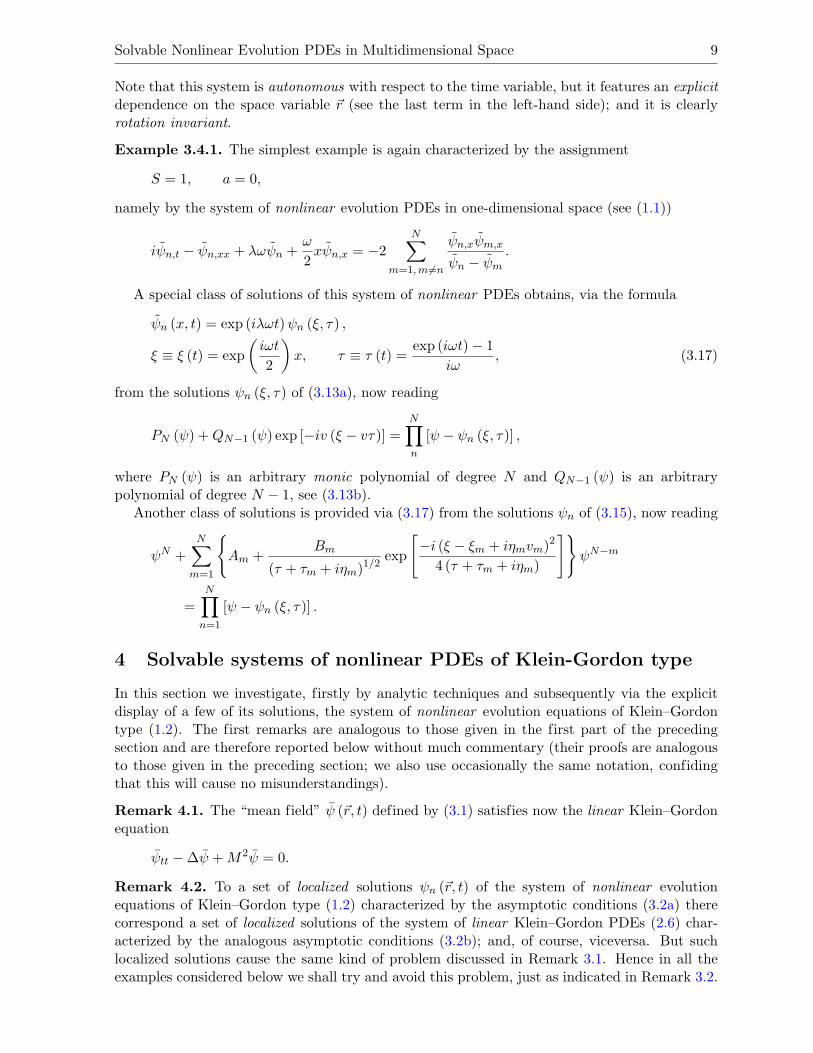
Figure 5.1.2. The absolute values of the ϕm (x, t) functions and the absolute values of the ψm (x, t)solutions for 0 ≤ t ≤ 20.

B1 = 1, B2 = 2, B3 = 3,

~v1 = (4√π, 0), ~v2 = (−2

√π, 2

√3π), ~v3 = (−2

√π,−2

√3π).

Here the periods in time of the three ϕm (~r, t) functions are chosen to be the same, T = 1/8,and the animation is performed on the time interval 0 ≤ t ≤ T , then closed in loop.

Fig. 5.1.1 is the first frame. To see the whole animation, please click on the following(external) link: http://www.emis.de/journals/SIGMA/2006/Paper088/Animation5.1.1.gif.

Example 5.1.2. The second animation corresponds to the Example 3.3.1, with S = 1, a = b =0, W (r) = V (r) = 0 and the ϕm (x, t) functions as in (3.14), namely

ϕm (x, t) = Am +Bm



4 (t+ tm + iηm)

],

with

A1 = 0, B1 = 0.5, x1 = 30, v1 = 0.5, η1 = 1, t1 = 0.8,A2 = −0.6, B2 = −0.9, x2 = 0, v2 = 1, η2 = 2, t2 = 0.4,A3 = 1.4, B3 = 0.8, x3 = −20, v3 = 0.5, η3 = 7, t3 = 1.

Here the animation is performed on the time interval 0 ≤ t ≤ 20.Fig. 5.1.2 is the first frame. To see the whole animation, please click on the following

(external) link: http://www.emis.de/journals/SIGMA/2006/Paper088/Animation5.1.2.gif.

5.2 Solutions of (1.2)

In this subsection we present three numerical solutions of (1.2) displayed as animations, twowith S = 2 and the last with S = 1.

Example 5.2.1. The first animation corresponds to the Example 4.3.1, with S = 2, a = b = 0,M = 0 and the ϕm (x, t) functions as in (4.4), with K = 4 and a very particular choice of thefunctions ϕm (x, y, t):

ϕm (x, y, t) = Am exp

−(x− x

(1)m − t

)2

am

+Bm exp

−(x− x

(2)m + t

)2

bm

http://www.emis.de/journals/SIGMA/2006/Paper088/Animation5.1.1.gif



Figure 5.2.1. The ϕm (~r, t) functions and the absolute values of the ψm (~r, t) solutions for 0 ≤ t ≤ 20.

+ Cm exp

−(y − y

(1)m − t

)2

cm

+Dm exp

−(y − y

(2)m + t

)2

dm

+ Em,

where

A1 = −3, B1 = 3, C1 = 0, D1 = 0, E1 = 0,A2 = 0, B2 = 0, C2 = −6, D2 = −3, E2 = 10,A3 = 6, B3 = 6, C3 = 3, D3 = 4.5, E3 = −12,a1 = 1.5, b1 = 1.3, c1 = 1.3, d1 = 1.6,a2 = 1.8, b2 = 1.2, c2 = 2, d2 = 1.6,a3 = 1.4, b3 = 1.5, c3 = 1.4, d3 = 1.2,

x(1)1 = −6, x

(2)1 = 7, y

(1)1 = 0, y

(2)1 = 0,

x(1)2 = 0, x

(2)2 = 0, y

(1)2 = 2.5, y

(2)2 = −1.5,

x(1)3 = −5, x

(2)3 = 6, y

(1)3 = −5.5, y

(2)3 = 4.5.

Here the animation is performed on the time interval 0 ≤ t ≤ 20.Fig. 5.2.1 is the first frame. To see the whole animation, please click on the following

(external) link: http://www.emis.de/journals/SIGMA/2006/Paper088/Animation5.2.1.gif.

Example 5.2.2. The second animation corresponds to the Example 4.3.2, with S = 2, a = b =0, M = 0 and the ϕm (~r, t) functions as in (4.5):

ϕm (x, y, t) = J0

(√(x− xm)2 + (y − ym)2

)[Am cos(t) +Bm sin(t)] + Cm,

where

A1 = 1, B1 = 0.1, C1 = 0, x1 = 5, y1 = 0,



Figure 5.2.2. The ϕm (~r, t) functions and the absolute values of the ψm (~r, t) solutions for 0 ≤ t ≤ 2π.

A2 = −1, B2 = 1, C2 = 3, x2 = −5/2, y2 = 5√

3/2,

A3 = 0.1, B3 = 1, C3 = −3, x3 = −5/2, y3 = −5√

3/2.

The ϕm (~r, t) functions are periodic in time with period T = 2π. The animation is performedon the time interval 0 ≤ t ≤ T , then closed in loop.


Example 5.2.3. The third animation corresponds again to the Example 4.3.1, with S = 1,a = b = 0, M = 0 and the ϕm (x, t) functions as in (4.4) with K = 2, and with a very particularchoice of the functions ϕm (x, t):

ϕm (x, t) = Am cos(x− t+Bm) + Cm cos(x+ t+Dm) + Em,

where

A1 = 1, B1 = 0, C1 = 3, D1 = 0.1, E1 = 0,A2 = 2, B2 = π, C2 = −1, D2 = π + 0.1, E2 = 5,A3 = −1, B3 = π/2 + 0.1, C3 = 2, D3 = π/2, E3 = −5.

The ϕm (x, t) functions are periodic in time with period T = 2π and periodic with respect tothe x variable with period L = π. The animation is performed on the time interval 0 ≤ t ≤ T ,then closed in loop.


6 Outlook

In future articles we plan to report additional investigations of these solvable (systems of)nonlinear evolution PDEs, and in particular to display visual animations of solutions of certainof these models in three-dimensional space.




Figure 5.2.3. The ϕm (x, t) functions and the absolute values of the ψm (x, t) solutions for 0 ≤ t ≤ 2π.

Acknowledgements

The final correction of this paper was done while both authors were taking part in a ScientificGathering on Integrable Systems and the Transition to Chaos at the Centro International deCiencias in Cuernavaca.

[1] Calogero F., Motion of poles and zeros of special solutions of nonlinear and linear partial differential equa-tions, and related “solvable” many body problems, Nuovo Cimento B, 1978, V.43, 177–241.

[2] Calogero F., A class of C-integrable PDEs in multidimensions, Inverse Problems, 1994, V.10, 1231–1234.

[3] Calogero F., Classical many-body problems amenable to exact treatments, Lecture Notes in Physics Mono-graph, Vol. 66, Berlin Heidelberg, Springer-Verlag, 2001.

[4] Calogero F., Isochronous systems, Monograph, 200 pages, to appear.

[5] Erdelyi A. (Editor), Higher transcendental functions, Vol. II, New York, McGraw-Hill, 1953.

[6] Gomez-Ullate D., Sommacal M., Periods of the goldfish many-body problem, J. Nonlinear Math. Phys.,2005, V.12, suppl. 1, 351–362.

[7] Mariani M., Calogero F., Isochronous PDEs, Theor. Math. Phys., 2005, V.68, 958–968.

Documents

Solvable Nonlinear Evolution PDEs in Multidimensional …emis.dsd.sztaki.hu/journals/SIGMA/2006/Paper088/sigma06-088.pdf · 2 F. Calogero and M. Sommacal which is rotation-invariant