Solutions to the Boltzmann Equation in the Boussinesq Regimefield, u and 8, are the Oberbeck-Boussinesq (OBE) equations (see refs. 4, 12), which we write as Here n is the kinematic

Journal of Statistical Physics, Vol. 90, Nos. 5/6, 1998

Solutions to the Boltzmann Equation in theBoussinesq Regime

R. Esposito,1 R. Marra,2 and J. L. Lebowitz3

Received June 6, 1997; final November 21, 1997

We consider a gas in a horizontal slab in which the top and bottom wallsare kept at different temperatures. The system is described by the Boltzmannequation (BE) with Maxwellian boundary conditions specifying the wall tem-peratures. We study the behavior of the system when the Knudsen number e. issmall and the temperature difference between the walls as well as the velocityfield is of order E, while the gravitational force is of order e2. We prove thatthere exists a solution to the BE for t E(0, t) which is near a global Maxwellian,and whose moments are close, up to order e2, to the density, velocity andtemperature obtained from the smooth solution of the Oberbeck-Boussinesqequations assumed to exist for t< t.

KEY WORDS: Boltzmann equation; hydrodynamic scaling; Boussinesqequation; Rayleigh-Benard convection.

1. INTRODUCTION

In the study of thermal convection phenomena the following system playsa paradigmatic role: a viscous heat conducting fluid between flat horizontalplates with the lower plate maintained at a temperature greater than theupper one. When the temperature difference between the plates is small, thestationary state is one in which the fluid is at rest with a linear temperatureprofile. When the temperature difference is made larger, the gravitationalbuoyancy force acting on the light, higher temperature fluid below, over-comes the effects of viscosity and a new stationary state of thermal Rayleigh-

1 Dipartimento di Matematica, Universita degli Studi di L'Aquila, Coppito, 67100 L'Aquila,Italy.

2 Dipartimento di Fisica, Universita di Roma Tor Vergata, 00133 Rome, Italy.3 Departments of Mathematics and Physics, Rutgers University, New Brunswick, New Jersey,

08903.

1129

0022-4715/98/0300-1129$15.00/0 C 1998 Plenum Publishing Corporation

Benard convection sets in. In typical experimental situations the variationsof temperature and density are small and the system is described in theBoussinesq approximation under which the Navier-Stokes equationsreduce to the Oberbeck-Boussinesq equations (OBE). This approximation,which is formulated on a phenomenological basis, gives quantitativelycorrect predictions in most cases.(1)

A justification of this approximation, based on introducing a scalingwhich leaves the Rayleigh number invariant is given in ref. 2 (see alsorefs. 3, 4). This approach follows the general strategy of taking into accountthe invariance, under appropriate scaling, of the hydrodynamical equations.Such considerations allow, for example, to derive the incompressibleNavier-Stokes equations from the compressible ones, as well as from micro-scopic and kinetic models.

The main aim of this paper is to derive the OBE starting from theBoltzmann equation (BE), which describes gases on the kinetic level, inter-mediate between the microscopic and the macroscopic. To go from thekinetics BE to a hydrodynamical one it is necessary to consider situationsin which the Knudsen number £, the ratio between the mean free path andthe size of the slab, is very small. It is well known that the inviscid Eulerequations correctly describe the behavior of this system for times of ordere-1 in the limit e->0.(5) To obtain the OBE we need to consider longertimes, of order e - 2 , so as to get the effects of viscosity and thermal conduc-tivity. To make this possible, we have to study the system in the incom-pressible regime, corresponding to macroscopic velocity fields of order e.(6)

This scaling would appear, at first sight, to require that the force G bescaled as e3 to be consistent with the incompressible regime, i.e. to get afinite force term in the equation for the velocity field. However, the case ofa conservative force is special from this point of view in that larger forcesare permissible. In fact we find that G has to be scaled as e2 in order tokeep the Rayleigh number finite.

We take the walls to be at fixed temperatures and impose a no-slipboundary condition for the velocity field at the hydrodynamic level. This ismodeled at the kinetic level by assuming that each particle colliding witha wall is reflected with a random velocity, distributed according to theequilibrium distribution at the temperature of that wall, i.e. we assumeMaxwellian boundary conditions.

Our solution of the BE is given in terms of a truncated expansion in ewhose leading term in the bulk is a global Maxwellian. The term of order e,denoted by f1, determines the hydrodynamic quantities which are close,up to order e2, to the density, velocity and temperature solutions of theOBE. Near the boundary, in a thin layer of size e, the hydrodynamicalapproximation is not correct and we provide a detailed description of the

1130 Esposito et al.

solution in this region. The initial datum is chosen to match the expansionup to order e2, to avoid a treatment of the initial layer which is more orless standard.

The validity of the expansion is established up to a time t such that theOBE have a sufficiently regular solution by estimating the remainder. Thisexpansion technique goes back to Hilbert, Chapman and Enskog; a rigorousproof of the hydrodynamic limit is given for the Euler case in ref. 5 andfor the incompressible Navier-Stokes case in ref. 6. In particular, in theabsence of gravity, the results of the present paper extend the ones of ref. 6to the case of a fluid confined in a domain with walls at different tem-peratures modeled by Maxwellian boundary conditions. The main techni-cal difficulty for such systems, even in the absence of an external force, isin dealing with the terms coming from the boundary conditions in theestimate for the remainder. The approach proposed in ref. 5, and used alsoin ref. 6, is based on the estimate of some Sobolev norm of the solutions.But in the presence of the boundaries this cannot be used because thederivatives of the solution may become singular at the boundaries. Weavoid the estimates of the derivatives by first looking for L2 estimates andthen improving them to Loo estimates. This technique was already used inrefs. 7 and 8 which concern essentially one-dimensional problems, i.e. acompressible fluid in a slab with the walls held at fixed temperatures underthe action of a force parallel to the walls in the stationary regime. Since weconsider here the fully three dimensional time dependent case we need tomodify the method to bound the Loo norm of the remainder by using a newmethod based on a result in ref. 9. This is presented in Section 4 and in theAppendix. A formal expansion including boundary layer corrections wasgiven earlier in ref. 10.

The case with a force perpendicular to the walls presents extra dif-ficulties stemming from the fact that we need good properties of thederivatives with respect to vz, the vertical component of the velocity, to getthe exponential decay of certain boundary layer terms and to control theremainder. Unfortunately, the derivative with respect to vz is singular atthe boundaries at v, = 0. To overcome this difficulty we have to decomposethe force into a part acting in the bulk only and a part acting only near theboundaries, decreasing to zero at a distance of order e. The Milne problemwe consider for the boundary layer terms involve these short range forcesand can be solved by using the result in ref. 11, where it is proven that thevz derivative is bounded in L2 and Loo norms locally, away from the boun-daries. This is enough to control the terms appearing in the equation forthe remainder and in the Milne problems for the higher order corrections.

While the above results are independent of the nature of the solutionof the OBE, we are only able to construct stationary solutions to the

Boltzmann Equation in Boussinesq Regime 1131


Boltzmann equation which correspond, at the hydrodynamic level, to thebehavior of the purely conducting stationary solution of OBE. This is dueto the fact that the methods in this paper are based on the perturbation ofa global Maxwellian and therefore require that the temperature differencebetween the plates be small, corresponding to having a small Rayleighnumber. We expect to be able to construct the purely conductive solutionof the Boltzmann equation for any Rayleigh number, even when the basichydrodynamic solution becomes unstable, by perturbing a Maxwelliancorresponding to the hydrodynamic solution. This involves many technicaldifficulties and will be discussed in a forthcoming paper. The hope is toextend these results to the convective solutions which appear for largervalues of the Rayleigh number.

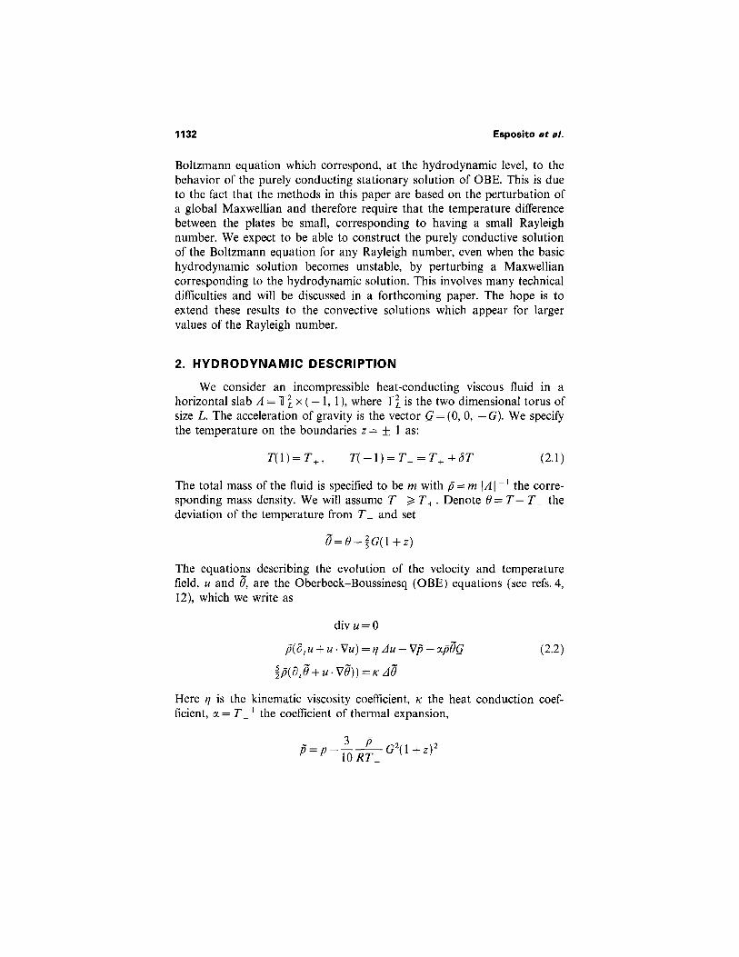
2. HYDRODYNAMIC DESCRIPTION

We consider an incompressible heat-conducting viscous fluid in ahorizontal slab A = T2

L x (— 1, 1), where T2L is the two dimensional torus of

size L. The acceleration of gravity is the vector G = (0, 0, — G). We specifythe temperature on the boundaries z = + 1 as:

The total mass of the fluid is specified to be m with p = m|A|-1 the corre-sponding mass density. We will assume T_ > T+. Denote 0= T— T_ thedeviation of the temperature from T_ and set

The equations describing the evolution of the velocity and temperaturefield, u and 8, are the Oberbeck-Boussinesq (OBE) equations (see refs. 4,12), which we write as

Here n is the kinematic viscosity coefficient, K the heat conduction coef-ficient, a = T-1 the coefficient of thermal expansion,

is kept fixed. We refer to ref. 2 for the detailed (formal) derivation of (2.2),(2.3), (2.4), (2.5) from the compressible Navier-Stokes in the limit e->0,while in next sections we will provide its rigorous derivation from theBoltzmann equation.

This scaling is a natural one in order to derive the OBE because, under it,the Rayleigh number Ra defined as

It can be proved that if u0 and 00 are smooth functions of x (i.e., withSobolev Hs(A)-norm finite for some s sufficiently large), then there is tdepending on the initial and boundary data such that the system (2.2),(2.3), (2.4) has a unique solution, at least as smooth as the initial data, for0 < t < t. We do not give the proof of this statement which is ratherstandard and refer to ref. 4 for details.

The regime under which the OBE are expected to be valid correspondto a low Mach number, a sufficiently weak gravity and a small differencebetween the temperatures of the top and bottom walls. To make thisprecise we introduce a space scale parameter e and rescale the variables asfollows:

for any (x, y) e T2L and any positive t.

Moreover, let r = p — p be the deviation of the density from thehomogeneous density p, let r = r + pG(1 +z)/T_. Then r is determined bythe Boussinesq condition

for any x e A, with div u0 = 0. The boundary conditions for this problemare

and p is the unknown pressure which arises from the incompressibility con-straint. The initial conditions are



We note that our equations do not coincide exactly with the usualOberbeck-Boussinesq (OBE) equations as given in refs. 4, 12 because ofthe term proportional to G in the boundary conditions for 9 and of thequadratic term in G in the definition of p. In the usual experimental condi-tions (see ref. 1) such terms are much smaller than the others, so one canneglect the effect of the variation of the density due to the gravitationalforce. If we denote by ps and Ts the solution of the stationary problem

with Ps = psTs and boundary conditions (2.1) the approximation corre-sponds to setting P s ~ P ( 1 ) = p(1) T(1) . In this way we would recover theusual OBE. We finally remark that the Boussinesq condition (2.5), whichis assumed as an "equation of state" in the usual discussions of theBoussinesq approximation (see ref. 3, 12), in our approach is just a conse-quence of the scaling limit (2.6).

3. KINETIC DESCRIPTION

We consider the BE for a gas between parallel planes. We keep thenotations of Section 2. To model the hydrodynamic boundary conditionswe choose the so called Maxwellian boundary conditions: when a particlehits the walls of the slab (z = — 1 or z = 1) it is diffusely reflected with avelocity distributed according to a Maxwellian with zero mean velocity andprescribed temperatures T_ and T+ respectively. In the language of kinetictheory this means that the accommodation coefficient equals one. Theabove prescription implies the impermeability of the walls, namely no par-ticle flux across the boundary is allowed. We introduce as scale parameter£ the Knudsen number. The height of the slab is 2e - 1 , hence in rescaledvariables z e [ — 1, 1 ]. we take for simplicity periodic conditions in the x, ydirection, and call

The BE rescaled according to (2.6) is

with

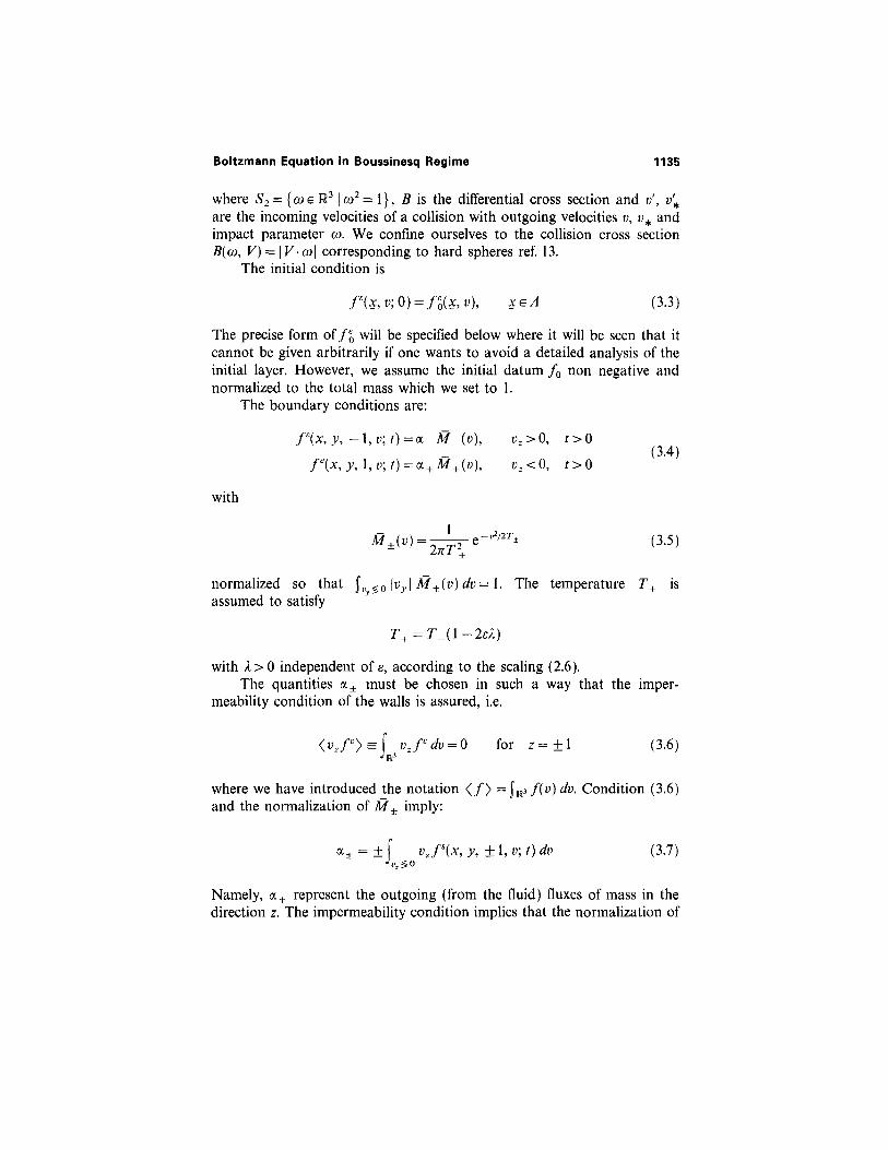
Namely, a± represent the outgoing (from the fluid) fluxes of mass in thedirection z. The impermeability condition implies that the normalization of

where we have introduced the notation <f> —fR3 f ( v ) d v . Condition (3.6)and the normalization of M ± imply:

with y>0 independent of e, according to the scaling (2.6).The quantities a± must be chosen in such a way that the imper-

meability condition of the walls is assured, i.e.

normalized so that fvy <o |vy| M ± ( v ) d v = 1. The temperature T+ isassumed to satisfy

with

The precise form of fo will be specified below where it will be seen that itcannot be given arbitrarily if one wants to avoid a detailed analysis of theinitial layer. However, we assume the initial datum f0 non negative andnormalized to the total mass which we set to 1.

The boundary conditions are:

where S2 = {w e R3| w2 = 1}, B is the differential cross section and v', v'*are the incoming velocities of a collision with outgoing velocities v, v* andimpact parameter w. We confine ourselves to the collision cross sectionB(w, V) = | V.w| corresponding to hard spheres ref. 13.

The initial condition is



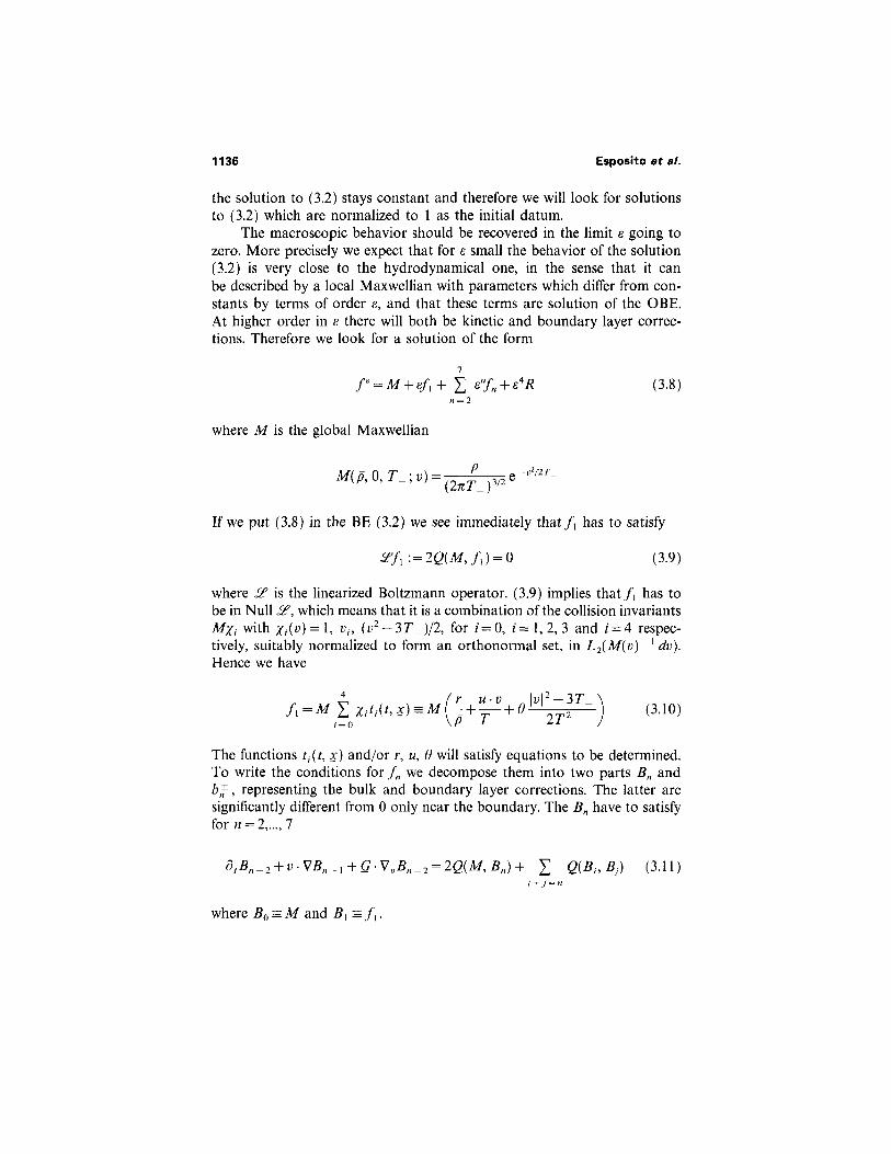
the solution to (3.2) stays constant and therefore we will look for solutionsto (3.2) which are normalized to 1 as the initial datum.

The macroscopic behavior should be recovered in the limit s going tozero. More precisely we expect that for e small the behavior of the solution(3.2) is very close to the hydrodynamical one, in the sense that it canbe described by a local Maxwellian with parameters which differ from con-stants by terms of order e, and that these terms are solution of the OBE.At higher order in e there will both be kinetic and boundary layer correc-tions. Therefore we look for a solution of the form

where M is the global Maxwellian

If we put (3.8) in the BE (3.2) we see immediately that f1 has to satisfy

where £ is the linearized Boltzmann operator. (3.9) implies that f1 has tobe in Null £, which means that it is a combination of the collision invariantsMXi with Xi(

v) = 1) vi, (v2 — 3T_)/2, for i = 0, i= 1, 2, 3 and i = 4 respec-tively, suitably normalized to form an orthonormal set, in L 2 ( M ( v ) - 1 dv).Hence we have

The functions t , ( t , x) and /or r, u, 0 will satisfy equations to be determined.To write the conditions for fn we decompose them into two parts Bn andb ±, representing the bulk and boundary layer corrections. The latter aresignificantly different from 0 only near the boundary. The Bn have to satisfyfor n = 2,..., 7

where B0 = M and B1 = f1.

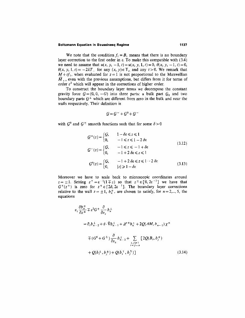
Moreover we have to scale back to microscopic coordinates aroundz = ± l . Setting z ± = e - 1 ( 1 + z ) so that z ± e [ 0 , 2 e - 1 ] we have thatG±(z±) is zero for z± e [28 ,2e - 1 ] . The boundary layer correctionsrelative to the wall z= ±1, b+, are chosen to satisfy, for n = 2,..., 5, theequations

with G° and G± smooth functions such that for some 8 > 0

We note that the condition f1 =B1 means that there is no boundarylayer correction to the first order in e. To make this compatible with (3.4)we need to assume that u(x, y, — 1 , t ) = u(x, y, 1, t) = 0, 0(x, y, —1, t ) = 0,0(x, y, 1, t)= — 2yT_ for any (x, y ) e T L and any t>0. We remark thatM + ef1, when evaluated for z = 1 is not proportional to the MaxwellianM+, even with the previous assumptions, but differs from it for terms oforder e2 which will appear in the corrections of higher order.

To construct the boundary layer terms we decompose the constantgravity force G = (0, 0, — G) into three parts: a bulk part G0 and twoboundary parts G± which are different from zero in the bulk and near thewalls respectively. Their definition is



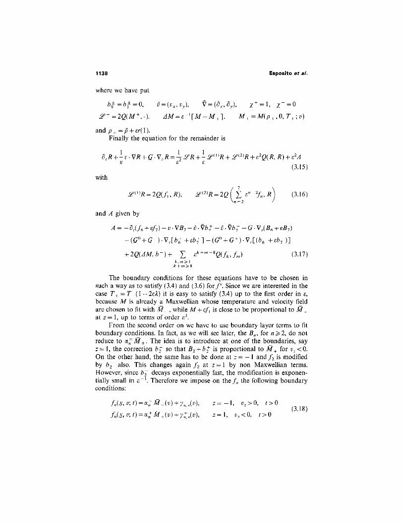
where we have put

and p + = p + er( 1).Finally the equation for the remainder is

with

and A given by

The boundary conditions for these equations have to be chosen insuch a way as to satisfy (3.4) and (3.6) for fe. Since we are interested in thecase T+ = T_( l — 2 e y ) it is easy to satisfy (3.4) up to the first order in e,because M is already a Maxwellian whose temperature and velocity fieldare chosen to fit with M_ , while M + ef1 is close to be proportional to M+

at z = 1, up to terms of order e2.From the second order on we have to use boundary layer terms to fit

boundary conditions. In fact, as we will see later, the Bn , for n > 2, do notreduce to a± M±. The idea is to introduce at one of the boundaries, sayz = 1, the correction b+

2 so that B2 + b2 is proportional to M+ for vz <0.On the other hand, the same has to be done at z = — 1 and f2 is modifiedby b2

- also. This changes again f2 at z = 1 by non Maxwellian terms.However, since b2 decays exponentially fast, the modification is exponen-tially small in e-1. Therefore we impose on the fn the following boundaryconditions:

because the Maxwellian M does not depend on x and t. This is equivalentto

to ensure the normalization of the solution. Note that this condition on Ris satisfied because it is true at time t = 0.

Outline of Solution

The equations for the /„ are coupled in a complicated way and haveto be solved in the proper sequence, which we now outline. The hydro-dynamical part of the bulk terms is determined by the solvability condi-tions for (3.11), that we get by multiplying (3.11) by xi, i = 0...4, integratingover velocity and using the fact that < Q ( f , g ) x i > =0. The solvability con-dition for (3.11) with n = 2 is

The initial conditions for R(x, v; 0) are chosen to be R(x, v; 0) = 0,z=+ l for simplicity. The initial values for the fn's are partly determinedby the procedure below, so that only their hydrodynamical part can beassigned arbitrarily. To remove such restrictions one would have to includean analysis of the initial layer, which we skip to make the presentation sim-pler. Finally we impose the conditions

Finally, to fulfil (3.4) we impose the following conditions on R:

with the functions y +e ( v ) exponentially small in e-1 and such that

(y +E V z > =0, to be specified later. Moreover



The first one is the usual incompressibility condition while the secondone becomes the Boussinesq condition (2.5), when one defines r = r +p ( G / T _ ) ( 1 + z ) . Once (3.24) are satisfied, we can deduce from (3.11) withn = 2 the following expression for B2, where L -1 denotes the inverse of therestriction of 3? to the orthogonal of its null space

The solvability condition for (3.11) with n = 3 is

and this produces the equations for u and 9. Let us fix i= 1, 2, 3 in (3.26).Then the first term gives the time derivative of pu. The second one reducesto — Gr after integrating by parts. Finally we write

The first term, as is well known, gives rise to the dissipative and transportterms in the second of (2.2), while the second one is the second ordercorrection to the pressure P2. The result is

Using the Boussinesq condition, the definitions of r and 0 and the relationbetween P2 and p of Section 2, we find (2.2)2 as in Section 2, with 77 givenby

To get the equation for the temperature, it is convenient to replace x4

in (3.26) by x4 = 1\2 [ v2 — 5T_)]. A simple computation, using the Boussinesqcondition, yields:

Since the coefficients t(2) can be chosen arbitrarily on the boundarieswe use them to compensate q2. To satisfy the impermeability conditionswe have to choose t(2) = 0 on the boundaries. The coefficients of thehydrodynamic part of B2 will, for i= 0, be determined by the compatibility

with boundary condition (at z =0) prescribing the incoming flux as theopposite of the non hydrodynamic part of B2 at z= — 1. The results inref. 11 tell us that the solution approaches, as z - -> oo a function q2 inNull L- . Thus we set b2=h — q2, which will go to zero at infinityexponentially in z - and will be the boundary layer correction we arelooking for.

In conclusion, we have

Summarizing our results so far: we have shown that, assuming u, p, 0satisfy the QBE (2.2), (2.3), (2.4), (2.5) up to a time t, the coefficients ti

entering in the definition of f1 are determined. Therefore, once initial andboundary conditions for the OBE are specified, f1 is completely determinedas a function of (t, x, v).

On the other hand the hydrodynamic part of B2 is not yet determined,but, by (3.28), div t ( 2 ) is determined in terms of r. Moreover, a combinationof t(2) and t4

(2) contributes to the pressure p which is determined by theOBE, so that these parameters are not independent.

The non-hydrodynamic part of B2 depends on the derivatives of r, u,9 which are in general different from zero on the boundaries. Therefore B2

violates the boundary conditions and we need to introduce b2 to adjustthe boundary conditions. We choose b2 by solving, for any t>0, theMilne problem

Finally, equation (3.26) with i = 0 gives

Collecting the above results we get (2.2) with K given by


In ref. 11 the following result is proved.

Theorem 3.1. (1) Suppose that for r>3 and some a'>0 thereare finite constants c1 and c2 such that

Consider the following Milne problem:

Iterating this procedure it is possible to find all fn. To prove that theterms in the expansion have the right properties we use the results in ref. 11for the solutions of the Milne problem with a force, that we state below.

Let F(z) = —a V ( z ) be a force vanishing at infinity such that V(x) andits derivative are bounded. Define

condition for n = 4. These are time-dependent non-homogeneous Stokesequations (linear second order differential equations) in a slab, togetherwith the b.c. t(2) = q21 , i= 1, 2, 4. Then t(2) is found up to a constant thatis chosen so that the total mass associated to f2 vanishes. Finally we get

1142 Esposito et at.

4. RESULTS IN THE TIME-DEPENDENT CASE

The main properties of the fn's are summarized in Theorem 4.1 below.

Theorem 4.1. Suppose that there is t>0 such that p(t), 0(t) andu(t) are smooth solutions of QBE, with | | V u ( t ) | | H s + | | V 0 ( t ) | | H s < q for suf-ficiently large s and 0<t < t. Then it is possible to determine functions fn,n = 2,..., 7 satisfying, for 0 < t < t, Eq. (3.11) and the conditions

for any a < c.

(3) If y :=supz e ( 0 , + o o )[ |F' |+ |F|] exists and is finite then for anyS > 0 and for y sufficiently small there exists a finite constant Cs such that

for some constant c/ and i = 3. Then there are finite constants c and c', suchthat

for any a < c'.

(2) Suppose that for fixed r > 3, l> 1 and some B > 0

Then there is a unique solution f eL o o(R+ x R 3 ) to the Milne problem(3.29)-(3.33). Moreover there exist constants c and c' such that / verifiesthe conditions:

1143Boltzmann Equation in Boussinesq Regime

where M+ =exp[ - V+(z + )] M+,_ -dz+V+ = e2G+, B2 is the non-hydro-dynamical part of B2 given by B2 = £-1[v. Vf1 + G. VVM- Q( f 1 , f1)].Finally q 2 ( v ; t) is the limit at infinity of the solution b2 of the same Milneproblem with boundary condition B2, as explained in the previous section.

The force G+ has been chosen smooth and vanishing as z+ goes to+ oo in such a way as to satisfy the assumptions on the force in Theorem3.1. Furthermore, for e small the force term (and its derivative) in (4.7) issmall. The boundary conditions verify (3.34) by the property of Jz-1 (seeref. 13). Hence, by Theorem 3.1, M - 1 / 2 b2

+ satisfy (3.35)-(3.39).

Proof. The proof is achieved by showing that every step of the proce-dure described in the previous section is correct, namely that the conditionson the source and on the boundary conditions for the Milne problems thatwe have to solve at each step are satisfied. Moreover we need to check thesolvability conditions for the Stokes equations.

Step 1. The first step is finding the boundary layer term b2 solvingfor any (x, y) e T2 the Milne problem for g2 = b2 /M+:

for h < 1 / ( 4 T _ ) . Here

Moreover, for any £ > 3 there is a constant c such that:



In the same way we construct b2 imposing the boundary condition inz- = 0 given by B2(x, y, -1, v; t).

Step 2. As explained above the coefficients ti(2), i=1,2,4 of the

hydrodynamical part of B2 are determined by the compatibility conditionfor n = 4

where

Proceeding as in the determination of the Boussinesq equation, we findnow a set of three linear time-dependent non-homogeneous Stokes equa-tions for ti

(2). The non-homogeneous terms depend on the third orderspatial derivatives of f1. We note that the non linear terms in the hydro-dynamic equations come from the quadratic term Q ( f 1 , f1) in (3.25), whilein (4.9) appears a term linear in B2. General theorems for the Stokes equa-tion assures the existence of a solution for the chosen boundary and initialconditions.

Step 3. Once B2 is completely determined, (4.9) gives the non-hydro-dynamical part of B3, B3. As before, we introduce the terms b3 to compen-sate B3 on the boundaries z= ± 1. The term b3 is found as a solution ofthe Milne problem for g3: ^/M+ g3 = b3

with source

and with boundary condition

We have to check that the source satisfies the conditions of Theorem 3.1.The condition (3.33) is true due to the properties of Q and to (3.32)

for b2 . The terms of the form Q(f, g) are bounded by means of the Gradestimates

and it is bounded because of (3.39), Theorem 3.1, that applies as shown inStep 1.

The first term in r.h.s. of (4.13) is bounded by observing that the timederivative of 62

- is a solution of the Milne problem we get by differentiating(4.7) with respect to time with boundary condition d,b2

-(0, v; t), vz>0,t>0.

The second term in r.h.s. of (4.13) is zero by construction forO<z < S so that

Since T_ = T + ( 1 +2ey) we have that |e - 1(M- M+ )/^/W_|r_1 < C | ( ( v 2 /T_) + 1 ) ^ M | r _ 1 .

The functions f1, and b2+ have bounded norm, hence the third term in

(4.11) is bounded. The first term in (4.11) is bounded by using the propertiesof the derivatives with respect to x and y of b2 assured by Theorem 3.1.

Step 4. B3 is constructed as in Step 2. Instead the Milne problem forb4 has to be discussed since in the source appear also derivatives of b2

+

with respect t and vz. We have for ^M + g4 = b4+ that

The second term in (4.11) is bounded in the same way

where |.| r :=|. | r , 0 , so that



Finally the condition (3.33) is satisfied since the velocity flux of thederivatives of b2 with respect to time and velocity is zero.

The terms /„ with higher n are constructed and bounded in the sameway. As a consequence, it is easy to see by using the preceding argumentsthat the term A in (3.15) satisfies the bound (4.5) and (4.2). This concludesthe proof of Theorem 4.1.

To complete the construction of a solution to the BE, we have toshow that the remainder is bounded in norm |.|l,h defined in (4.6).The remainder has to satisfy (3.15) and the conditions (3.20) and (3.21)with <yn,e

±Bvz> =0. Moreover R has to satisfy

which implies aR = ± f v z < 0 v z R ( ± 1 , v ; t) dv. To construct the solution of(3.15), (3.20), (3.21) and (4.14) we first deal with the following linear initialboundary value problem: given D on T2 x [ -1, 1 ] x R3, find R such that

with the same initial and boundary conditions as before.Once one obtains good estimates for the solution of this linear

problem, the non linear problem is solved by simple Banach fixed pointarguments, for small e. This allows to conclude the existence of the solutionfe and its convergence to the solution of the OBE.

Solution of Linear Problem

We consider the linear problem (4.15) with a given D satisfying<y z D> =0. Put R = MO. Therefore the equation for O is

where D = M- 1/2D, M = M exp[ eG(z + 1 )/T_ ] and

The boundary and initial conditions are


where

Introduce the L2 norm as

We now give the L2 bound for O and then we provide the Loo bound.

Theorem 4.2. The solution of the linear problem (4.16), (4.17)satisfy the bound

with

Proof. Multiplying (4.16) by O and integrating on Q x R3 we have

To bound the boundary terms in the second line of (4.19), we proceed asfollows. We consider first the more difficult term

In Appendix we prove that the r.h.s. of (4.23) is bounded as follows:let t1 be any time in (0, t]. Then

The same argument shows that ( v z O 2 ( x , y, — 1, v; t)> is non positivebecause

Using this bound and (4.21) in (4.20) we find

Using the relation between M in z= +1 and M+, the normalization ofM+, and the relation T+ = T _ ( 1 — 2ey), we get, after a straightforwardcomputation,

By the Schwartz inequality,


1150 Esposito at al.

We recall the following crucial properties of the linearized Boltzmannoperator L (see for example ref. 13):

with K an integral operator and v a smooth function. Moreover, for hardspheres, there are two constants v0 and v1 such that

(2) There is a constant C>0 such that

with the usual decomposition O = O + 0, with P and <P the non-hydrodynamical and the hydrodynamical part of 0 respectively.

To estimate the operators L1 and L2 we will use the following estimateon the collision operator Q (see for example ref. 14): for any MaxwellianM and for any y e [ — 1, 1 ]

This inequality and the bounds on the fn's imply the following bounds:

Note that the presence of the product ||^v0|| ||$|| depends on the factthat L1 and L2 are both orthogonal to the collision invariants.

We integrate (4.19) in time between 0 and t1, and recall that0(x, v,0) = 0. With the notation ( ., t), we get

A and Q are defined in (3.1).We call p 1 ( x , v ) the characteristics of the equation

Loo Bound

Let us give some notation:

In conclusion, by the use of the Gronwall lemma, for £ sufficiently small,we get:

is valid for any positive e, x, y. We apply it with x = ||v $ ||, y = ||<P|| andsuitable constants c1 and c2. We get

The last line in (4.29) derives from the bound (4.24). The first term in thesecond line is due to the bounds (4.27) and (4.28). Moreover||M- 1/2f1|| < C by the regularity of the solutions of the macroscopic equa-tions for 0<t<t and \ \M - 1 / 2E 7

n = 2 f n | | <C by Theorem 4.1.The following elementary inequality



given by

and, for fixed t, define t as the last time, before t, in which the charac-teristics passing by (x, v) at time t is in a point (z, w) such that ( t - , z, w) edS (see ref. 15, p. 44-48).

Given smooth functions H, v on S and h in dS, consider the initialboundary value problem

The solution of this problem is written as

We introduce the norm

and denote by Lp ,q the corresponding space. We define the operator Ns as

We assume that v corresponds to the collision rate for hard spheres, i.e.

Then Ns satisfies the estimate

where

Hence the result.This Lemma will be used also for p = + oo and q > d to control the

(oo, q)-norm of N's f in terms of (q, oo)-norm of the solution of (4.36).We write (4.16), (4.17) in the form (4.34), (4.35) with

we get

With one more change of variables

where we have put i = s — t. We have under the change (4.42)

Proof. Consider the following change of variables v -> y:


The following lemma allows to bound the Lp,q norm of Ns f in termsof the Lq,p norm of f. It is a generalization to the case with a constant forceof the theorem of Ukai and Asano.(9)

Lemma 4.3. Assume x, veRd and let 1<q, p<+oo and a =( 1 / q ) - ( 1 / p ) . Then


Here the v' are defined analogously to v as

Finally we set v = v + ev1 + £2v2 and it is immediate to check that v satisfiesthe assumption (4.39).

We have the following

Theorem 4.4. Let d, 1/2 — 1 /d< 1/q,

Proof. By (4.36) we get

In the last term we substitute for <& its expression (4.36) so that

To estimate the terms containing K we use the following Lemma whoseproof is given in ref. 9.

Lemma 4.5. Let LsY the spaces of functions f(v) such that

with y e R. Let 1 < s< r < oo and n 0 = 1 — ( 1 / s ) + ( 1 / r ) . Then the operator KmapsL; into Ly +n if ( 1 / s ) - ( 1 / r ) <(2/d) and n<n0.


Substituting (4.47) in (4.46) we get

Using (4.40) and the bound f t ds exp[ - e - 2 v 0 ( t - s ) ] < Ce2, thefirst term in the r.h.s. of (4.48) is estimated as Cs2 sup0<t<t ||H'||oo,q. Thesecond term is dealed with by using (4.40) to get rid of the time integralsso that we gain a factor e2. By Lemma 4.5 the operator K maps Loo in itselfso that the final bound for this term is again Ce2 sup0<t<t ||H'||oo,q. Webound the last term in (4.48) by using Lemmas 4.3 and 4.5 as follows.

To get the first inequality we have used (4.40) and Lemma 4.3. Thesecond step is based on Lemma 4.5 to replace the Loo norm on the velocitywith the L2 norm, by taking r = + oo, s = 2, y = 0. We pass from the secondline of previous inequality to the third one using again Lemma 4.3 toexchange the exponents for space and velocity introducing a factor( e / ( s - s ' ) ) d B , with B= 1/2-1/q, while (4.40) produces the factorexp[—v0(s —s')/e2]. Finally Lemma 4.5 again, with r = q, s = 2 and y = 0,gives the bound in terms of the L2 norm in space and velocity.

To get convergence of the /-integral we need Q<B< 1/d, so we haveto choose q > d, 1/2 — 1/d<1/q. From the time integrations we get a factor

We remark that the characteristics p which is on the boundary z = 1with velocity v such that vz>0 at time t- — t had to start either from somepoint in the bulk or from the boundary z = — 1. In the first case wehave h = 0 in (4.51) otherwise we get h = 0(x,y, — 1 , v ; t ) for t z >0. In

Equation (4.36) allows to express aR in terms of P(x, y, — 1 , v , t ) ,vz<0 and H. In fact by (4.36)

If r_ = t then h = <P(x, v; 0) = 0; if T_<t then h = <P(x, y, ± 1, v; t), incorrespondence of v z < O and ( p _ T ( x , v ; t ) ) z = ± 1 . The boundary condi-tions on 0 are given by (4.17) with

Now we control the boundary terms. First, we observe that by using(4.40) and Lemma 4.5 as we did for the second term in (4.48) we canestimate the second term in (4.50) as C sup0<s<t ||Ns h||oo,q . Hence we areleft with the first term in (4.50). We recall that the meaning of the bound-ary condition h is as follows: define

£4-2(u+u) with u = d/q, u1 = dp. Combined with the prefactor e(u+u) itproduces e4-(u+u). But u +u' =d/2 so that the factor we gain is e 4 - d / 2

In conclusion



the latter case it is shown in the Appendix that the integral f ' t -dsv( < p s - t ( x , y, — 1 , v ) ) is bounded from below by Ce. As a consequence, wecan estimate the exponential in the first row of (4.51) as e-c/E.

We exploit the same argument to deal with aR and use (4.36) to repre-sent <t> on the boundary z = — 1. There is a difference with respect to theprevious case: due to the presence of the force the characteristic q> whichis on the boundary z = — 1 with velocity v, v z<0 at time t- — t can startfrom the bulk, from the boundary z = 1 with negative v. or from theboundary z— — 1 with positive v2. In the Appendix it is shown that in thelatter case the exponential factor in the first row of (4.51) allows to gain afactor Ce2.

We discuss explicitely the bound for aR. The case of aR is dealt within the same way. By using the representation (4.36) we get

where ||C||OO,Q :=sup^x,y e an [f dv Cq]1/q. The first step is obtained from theinequality


As explained before, to get a bound of the last term in (4.52) in terms ofthe L2 norm we need to iterate the procedure and use again the representa-tion formula (4.36) in the last term

In this way all the terms in (4.53) are analogous to terms already discussedin the first part of the proof but the term containing h. The problem withthis term is that it can be estimated in terms of the Loo norm of 0 but weneed to gain a small factor and Ns- cannot provide it. Hence we have torepeat the previous argument and use (4.36) to represent 0 on the bound-ary in terms of the function evaluated on the point on the boundaryreached after a finite amount of time.

We get

By using the properties of Ns and K and the bounds on the integral in theexponential as discussed before the second term in (4.54) is bounded bye2||*||oo,q.

Finally we get

By (4.40) and Lemma 4.5 (used with r= +00 and s replaced by q), forq > d/2 we have


Now we can apply all the previous arguments to get the following estimatefor the boundary term in (4.50)

Finally by (4.50) and (4.30) we have

This concludes the proof of Theorem 4.4.To get the L°° bound for 3

Proof. By (4.36) we have

Hence, for e small

Finally the regularity property of the hydrodynamic solution and Theorem4.1 give

where Q + is the gain term of the collision operator.By using (4.59) and the definitions of Ki, i= 1, 2 we get

The boundary term |h|0< C |aR |oo + |aR |oo + |C|o has been estimatedbefore by using (4.56). The containing H' will be bounded using the Gradestimate

Hence

Because of the factor (1 + | v | ) r in the definition of |.|r and of the bounded-ness of the space domain, if r > 3 we have

By (4.57) we get

1160 Esposito et gl.


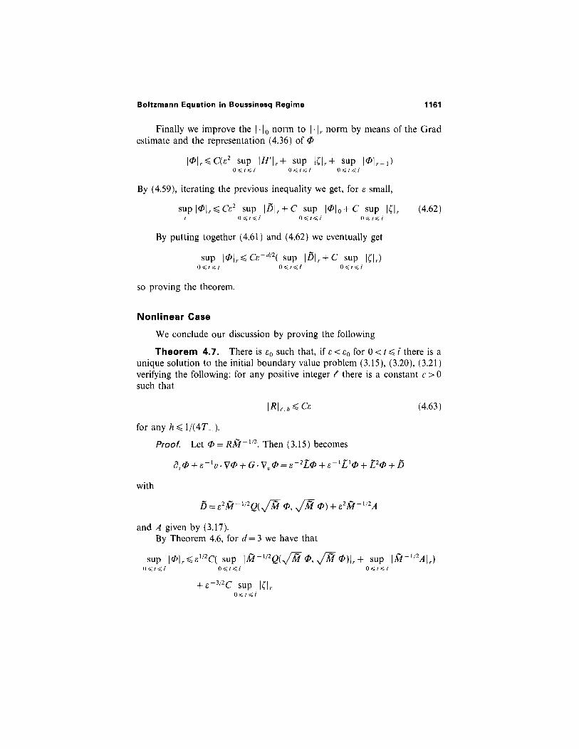
Finally we improve the | . |0 norm to | . |r norm by means of the Gradestimate and the representation (4.36) of <t>

By (4,59), iterating the previous inequality we get, for e small,

By putting together (4.61) and (4.62) we eventually get

so proving the theorem.

Nonlinear Case

We conclude our discussion by proving the following

Theorem 4.7. There is e0 such that, if e < e0 for 0 < t < t there is aunique solution to the initial boundary value problem (3.15), (3.20), (3.21)verifying the following: for any positive integer f there is a constant c>0such that

for any h < 1 / ( 4 T _ _ ) .

Proof. Let 0 = RM-1/2. Then (3.15) becomes

with

and A given by (3.17).By Theorem 4.6, for d = 3 we have that

with M ± ( v ) given by (3.5) and a± now independent on x, y and t, givenby (3.7), so that f e satisfies (3.6).

We construct the solution in the form (3.8) with fn to be determinedaccording to a bulk and boundary layer expansion. These terms are com-puted as in the time-dependent case and a theorem similar to Theorem 4.1can be stated also in this case. We only discuss the remainder equation

The boundary conditions are:

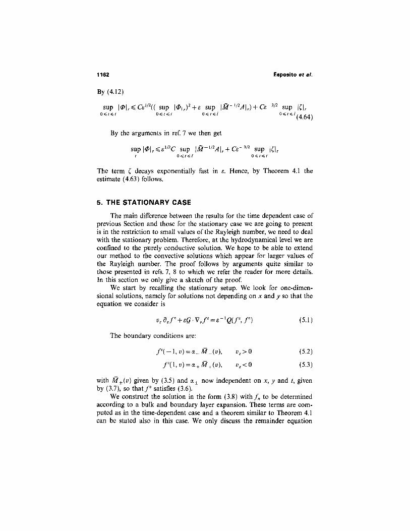
The term ( decays exponentially fast in e. Hence, by Theorem 4.1 theestimate (4.63) follows.

5. THE STATIONARY CASE

The main difference between the results for the time dependent case ofprevious Section and those for the stationary case we are going to presentis in the restriction to small values of the Rayleigh number, we need to dealwith the stationary problem. Therefore, at the hydrodynamical level we areconfined to the purely conductive solution. We hope to be able to extendour method to the convective solutions which appear for larger values ofthe Rayleigh number. The proof follows by arguments quite similar tothose presented in refs. 7, 8 to which we refer the reader for more details.In this section we only give a sketch of the proof.

We start by recalling the stationary setup. We look for one-dimen-sional solutions, namely for solutions not depending on x and y so that theequation we consider is

By the arguments in ref. 7 we then get

By (4.12)


Sketch of the Proof. We follow the strategy of the previous section:first we get a L2 bound and then the Loo bound. In the present case we

Then there are A 0 > 0 and e 0>0 such that, if A < A 0 and e<e0, thereis a stationary solution to the boundary value problem above such that

with r and 0 the thermal conduction solution of the OBE corresponding tothe temperatures T_ and T+ = T(1 — 2eA), namely

The theorem below summarizes the results about the existence ofstationary solutions.

Theorem 5.1. Let M be the Maxwellian with parameters p, Tand vanishing mean velocity. Put

The boundary conditions on R are given by (3.20), (3.21). R satisfies thenormalization condition (3.22) and the vanishing flux condition

with J2?(1) and £(2)R defined in (3.16). Moreover, A is given by

because its solution requires a different technique. This equation has theform


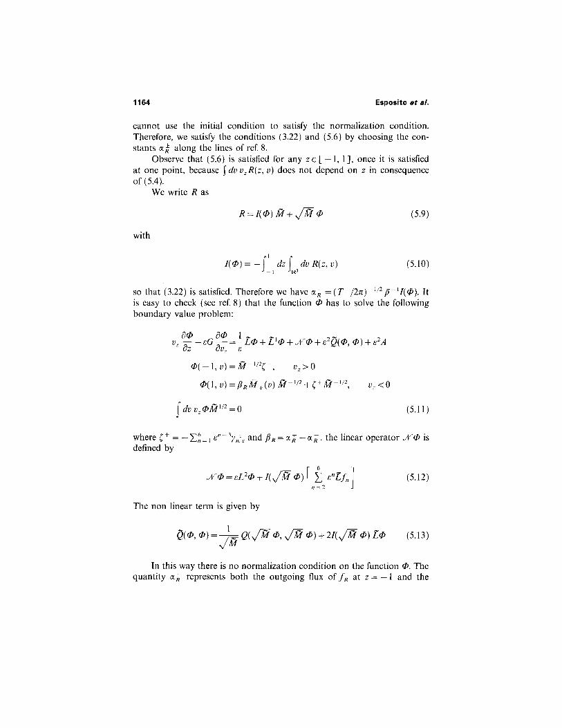
In this way there is no normalization condition on the function 0. Thequantity aR represents both the outgoing flux of fR at z = — 1 and the

The non linear term is given by

where C+ = — En = 1 en-3y+n,e and BR = aR —aR . the linear operator N<t> is

defined by

so that (3.22) is satisfied. Therefore we have aR = ( T _ / 2 n ) - 1 / 2 p - 1 I ( < t > ) . Itis easy to check (see ref. 8) that the function <P has to solve the followingboundary value problem:

with

cannot use the initial condition to satisfy the normalization condition.Therefore, we satisfy the conditions (3.22) and (5.6) by choosing the con-stants aR along the lines of ref. 8.

Observe that (5.6) is satisfied for any ze [ — 1, 1], once it is satisfiedat one point, because f dv vzR(z, v) does not depend on z in consequenceof (5.4).

We write R as



integral of R over z and v. The constant BR is determined so that R satisfiescondition (5.6) at the point z= 1, i.e.

To construct the solution of (5.11), we first consider the followinglinear boundary value problem: given D on [ — 1, l ] x R 3 and £* on{ve R3 s.t. v z < 0 } , find R satisfying

and the last three conditions (5.11).As usual we introduce the hydrodynamic and the non-hydro-

dynamic part of 0 respectively. Multiplying (5.15) by <t> and integratingover velocity, we have

By integrating over z, using (4.25), (4.27) and (4.28) we get

Here ||*||2 = f 1_1 dz f dv j2v. One can check (see ref. 8) that the l.h.s. of thisinequality is positive. Therefore we get

Using the inequality xy <kx2 + y2/4k with x= ||||, y = e ||0|| and asuitably small k, we find

To bound the hydrodynamical part, we multiply (5.15) by v,Y,,yi = M xi, i = 2 and integrate over [ - 1, z] x R3.

Note that the only point where we need X small is in the step from (5.18)to (5.19).

Combining (5.16) and (5.19) we get

so that for A small enough we get

with B a non-singular matrix. This allows to estimate Hi and hence =0, we can decompose , we get



Loo Bounds

To write the integral form of the linear equation (5.15) we follow theapproach in ref. 11. the notation is as follows: The "total energy" isE(z, v) = v2/2 + V(z) with V(z) = eG(z + 1). The lines with fixed E are thecharacteristic curves of the equation

For E(z, v) > V(z') we define

Moreover call z + (z, v) the function implicity defined by the equation

Finally put

Consider the equation

with boundary conditions

The solution of (5.21) can be written in an integral form as: for v, >0:

The definition of T is given in a similar way.By slightly modifying the proof in ref. 11 to take into account the

factor s it is possible to prove the following Lemmas (see also ref. 7).

where

We can write the previous formulas in a compact form as

for vs<0 and E> V ( 1 ) :

for vz<0 and E< V ( 1 } )


Finally (5.30) implies

Noting that ||v-1/2D|| < | v - 1 D | 3 and using (5.19) we get

and h ± ( ± 1 , v ) given by (5.11). Combining these Lemmas and usingthe properties of the operator L one gets

Theorem 5.4. There exists a constant C such that for any r < 3 thesolution of (5.15) verifies

We write (5.14) in the form (5.21) with

Here

Lemma 5.3. For any d > 0 and for any r > 2 there is a constant Cs

such that

Here

Lemma 5.2. For any integer r>O there is a constant c such thatthe integral operator T satisfies the following inequality,


Using now the form of Hin (5.28)

Finally, using again the Schwartz inequality and recalling the expression ofBR in (5.14) we get

we get

with s ± = £ ± M - 1 / 2 and |s± | = supvy < o,z | s ± ( v ) | . By (5.25), using theSchwartz inequality and

The term containing h involves BR which still depends on <P. Toestimate it, we follow the method in ref. 8.

Equation (5.25) allows to express BR in terms of T H and the restric-tion of P( — 1, v) to vz > 0. We have the estimate


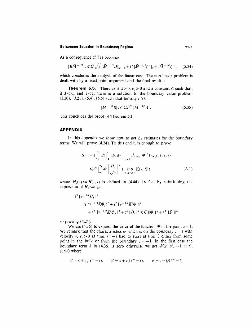
so proving (4.24).We use (4.36) to express the value of the function <t> in the point z = 1.

We remark that the characteristics q which is on the boundary z = 1 withvelocity v, vz>0 at time t- — t had to start at time 0 either from somepoint in the bulk or from the boundary z = — 1. In the first case theboundary term h in (4.36) is zero otherwise we get P(x', y', — 1 , v ' ; t ) ,v'z > 0 where

where H , ( . ) : = H ( . , t ) is defined in (4.44). In fact by substituting theexpression of H, we get

APPENDIX

In this appendix we show how to get L2 estimates for the boundaryterms. We will prove (4.24). To this end it is enough to prove

This concludes the proof of Theorem 5.1.

which concludes the analysis of the linear case. The non-linear problem isdealt with by a fixed point argument and the final result is

Theorem 5.5. There exist A > 0, EO > 0 and a constant C such that,if y < A0 and e<e0 there is a solution to the boundary value problem(3.20), (3.21), (5.4), (5.6) such that for any r>O

As a consequence (5.31) becomes



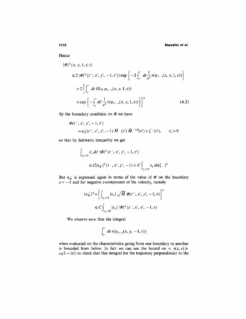
Hence

By the boundary condition on $ we have

so that by Schwartz inequality we get

But aR is expressed again in terms of the value of £ on the boundaryz = — 1 and for negative z-component of the velocity, namely

We observe now that the integral

when evaluated on the characteristics going from one boundary to anotheris bounded from below. In fact we can use the bound on v, v(x, v) >c0(l + |v|) to check that this integral for the trajectory perpendicular to the

where

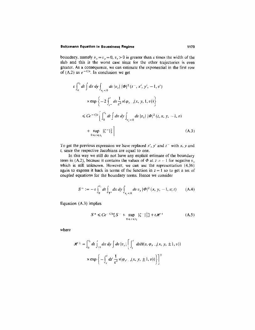
Equation (A.3) implies

To get the previous expression we have replaced x', y' and t with x, y andt, since the respective Jacobians are equal to one.

In this way we still do not have any explicit estimate of the boundaryterm in (A.2), because it contains the values of P at z= — 1 for negative vz

which is still unknown. However, we can use the representation (4.36)again to express it back in terms of the function in z = 1 so to get a set ofcoupled equations for the boundary terms. Hence we consider

boundary, namely vx = vy = 0, vz > 0 is greater than e times the width of theslab and this is the worst case since for the other trajectories is evengreater. As a consequence, we can estimate the exponential in the first rowof (A.2) as e - c / e . In conclusion we get


The other trajectories give a larger value to this integral.

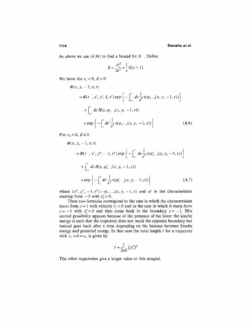
where (x", y " , — 1 , v " ) = (pt-_,(x, y , — 1 , v ) and p' is the characteristicsstarting from -1 with v" > 0.

These two formulas correspond to the case in which the characteristicsstarts from z = 1 with velocity vz'< 0 and to the case in which it starts fromz= — 1 with v">0 and then come back to the boundary z= — 1. Thissecond possibility appears because of the presence of the force: the kineticenergy is such that the trajectory does not reach the opposite boundary butinstead goes back after a time depending on the balance between kineticenergy and potential energy. In that case the total length l for a trajectorywith vx = 0 = vy is given by

For vz<0, E<0

We have: for vz<0, E>0

As above we use (4.36) to find a bound for S . Define


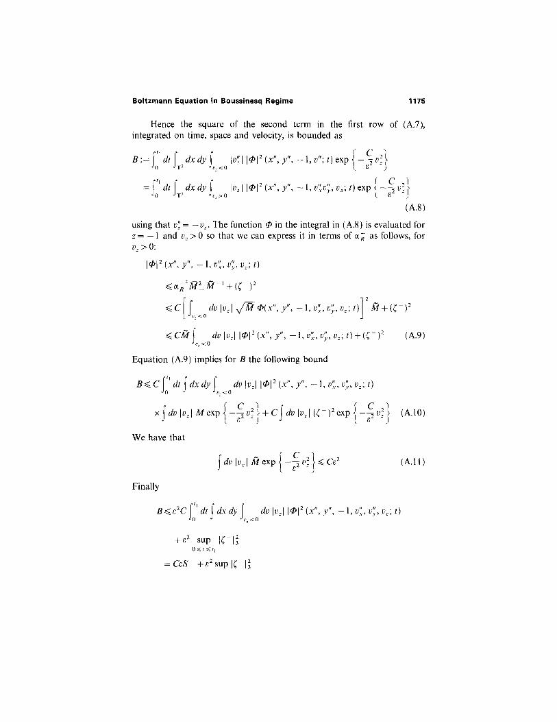
Finally

We have that

Equation (A.9) implies for B the following bound

using that v",= — v,. The function <t> in the integral in (A.8) is evaluated forz = — 1 and v, > 0 so that we can express it in terms of aR as follows, forv. > 0:


Hence the square of the second term in the first row of (A.7),integrated on time, space and velocity, is bounded as

To conclude the argument we now provide an estimate for H. By theSchwartz inequality applied to the integral over s, we have

Putting together (A.5) and (A.14) we get

where 2P = 3f + + 3? . This implies, for e small,

Summarizing we can write

The contribute of the first term in (A.7) to S is

Esposito et al.1176


Consider the term

and the following change of variables (t, vz) -> (£, w)

whose Jacobian is e |vz|-1. Denote also by t(£) the inverse of £(t). We have

Hence

ACKNOWLEDGMENTS

Research supported in part by AFOSR Grant 95-0159, and by CNR-GNFM and MURST. We also wish to thank the warm hospitality of theIHES, Bures-sur-Yvette, where some of this work was done.

REFERENCES1. P. G. Drazin and W. H. Reid, Hydrodynamic Instability (Cambridge Univ. Press,

Cambridge, 1981).


2. R. Esposito and R. Marra, Incompressible fluids on three levels: hydrodynamic, kinetic,microscopic, Mathematical Analysis of Phenomena in Fluid and Plasma Dynamics (RIMS,Kyoto, 1993).

3. J. M. Mihaljan, A rigourous exposition of the Boussinesq approximation applicalbe to athin layer of fluid, Astrophys. J., 136:1126-1133 (1962).

4. D. D. Joseph, Stability of Fluid Motions (Springer-Verlag, Berlin, 1976).5. R. E. Caflisch, The fluid dynamic limit of the nonlinear Boltzmann equation, Commun. on

Pure and Applied Math. 33:651-666 (1980).6. A. De Masi, R. Esposito, and J. L. Lebowitz, Incompressible Navier-Stokes and Euler

limits of the Boltzmann equation, Commun. Pure and Applied Math. 42:1189-1214 (1989).7. R. Esposito, J. L. Lebowitz, and R. Marra, Hydrodynamic Limit of the Stationary

Boltzmann Equation in a Slab, Commun. Math. Phys. 160:49-80 (1994).8. R. Esposito, J. L. Lebowitz, and R. Marra, The Navier-Stokes limit of stationary solu-

tions of the nonlinear Boltzmann equation, J. Stat. Phys. 78:389-412 (1995).9. S. Ukai and K. Asano, Steady solutions of the Boltzmann equation for a flow past an

obstacle, I. Existence, Arc. Rat. Mech. Anal. 84:249-291 (1983).10. C. Bardos, R. Caflisch, and B. Nicolaenko, Thermal layer Solutions of the Boltzmann

Equation, Random Fields: Rigorous Results in Statistical Physics. Koszeg (1984), J. Fritz,A. Jaffe and D. Szasz, eds. (Birkhauser, Boston, 1985).

11. C. Carcignani, R. Esposito, and R. Marra, The Milne problem with a force term, preprint(1996).

12. J. Boussinesq, Theorie analytique de la chaleur (Gauthier-Villars, Paris, 1903).13. C. Cercignani, R. Illner, and M. Pulvirenti, The Mathematical Theory of Dilute Gases

(Springer-Verlag, New York, 1994)14. F. Golse, B. Perthame and C. Sulem, On a boundary layer problem for the nonlinear

Boltzmann equation, Arch. Rat. Mech. Anal. 104:81-96 (1988).15. N. B. Maslova, Nonlinear evolution equations: kinetic approach (World Scientific, 1993).

Documents

Solutions to the Boltzmann Equation in the Boussinesq Regimefield, u and 8, are the Oberbeck-Boussinesq (OBE) equations (see refs. 4, 12), which we write as Here n is the kinematic