Embed Size (px)
Citation preview

Solutions to Schrödinger's equation for spherical potential wells:
Modelling the Atomic Nucleus
and the H atom electron
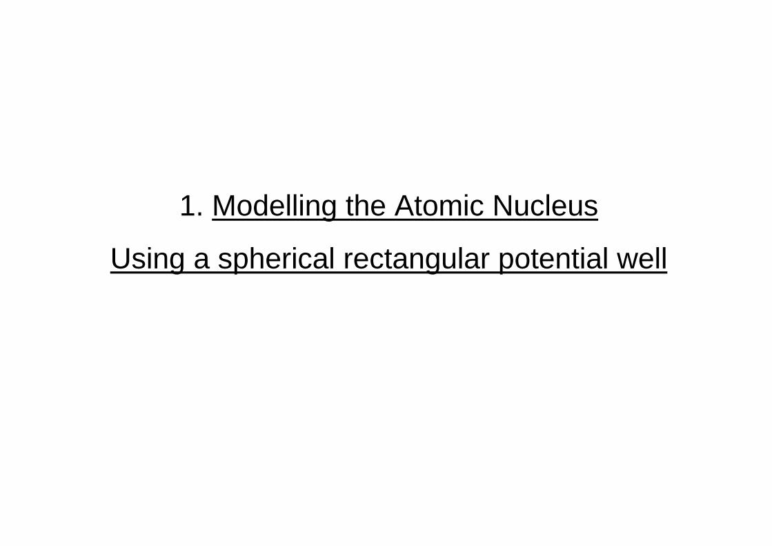
1. Modelling the Atomic Nucleus
Using a spherical rectangular potential well

q
1D finite rectangular well
0
−V0
(3D) finite spherical rectangular well
f
V(r) = 0 for r ≥ R
V(r) = −V0 for r < R
0 Rr
r r
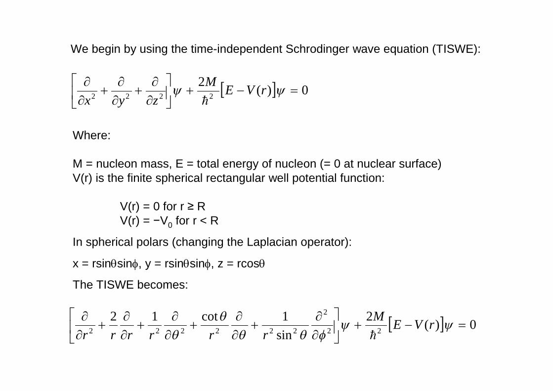
We begin by using the time-independent Schrodinger wave equation (TISWE):
[ ] 0 )(2
2222 =-+úû
ùêë
鶶
+¶¶
+¶¶ yy rVE
Mzyx h
Where:
M = nucleon mass, E = total energy of nucleon (= 0 at nuclear surface)V(r) is the finite spherical rectangular well potential function:
V(r) = 0 for r ≥ RV(r) = −V0 for r < R
In spherical polars (changing the Laplacian operator):
x = rsinqsinf, y = rsinqsinf, z = rcosq
The TISWE becomes:
[ ] 0 )(2
sin1cot12
22
2
222222 =-+úû
ùêë
鶶
+¶¶
+¶¶
+¶¶
+¶¶ yy
fqqq
qrVE
Mrrrrrr h

Separation of variables gives:
[ ]
[ ] )1(sin
1cot
1)(
22
:)RYrby (multiply
0)(2
sincot2
:
),()(),,(
2
2
22
2
2
2
2
22
2
22
2
2222
2
22
2
+=úû
ùêë
鶶
+¶¶
+¶¶
-=-++
=-+¶¶
+¶¶
+¶¶
++
=
llYYY
YrVE
MrdrdR
Rr
drRd
Rr
RYrVEMY
rRY
Rr
YrR
drdR
rY
drd
Y
gives
YrRr
fqqq
q
fqqq
q
fqfqy
h
h
Where we have set each side equal to a constant which we have designated l(l+1) for later convenience.
[ ]
0)1(sin
1cot
1
)1()(22
2
2
22
2
2
2
2
22
=++úû
ùêë
鶶
+¶¶
+¶¶
+=-++
llYYY
Y
llrVEMr
drdR
Rr
drRd
Rr
fqqq
q
h(1)
(2)
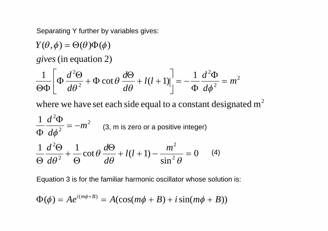
Separating Y further by variables gives:
0sin
)1(cot11
1
m designatedconstant a toequal sideeach set have wewhere
1)1(cot
1
2)equation (in
)()(),(
2
2
2
2
22
2
2
22
2
2
2
=-++Q
Q+
-=F
F
=F
F-=ú
û
ùêë
é++
QF+
QF
QF
FQ=
qqq
q
f
fqq
q
fqfq
mll
dd
dd
mdd
mdd
lldd
dd
gives
Y
(3, m is zero or a positive integer)
(4)
Equation 3 is for the familiar harmonic oscillator whose solution is:
))sin()(cos()( )( BmiBmAAe Bmi +++==F + fff f
0sin
)1(cot11
2
2
2
2
=-++Q
Q+
QQ qq
mll
dd
dd
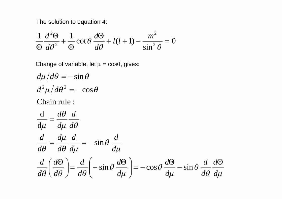
The solution to equation 4:
Change of variable, let m = cosq, gives:
mqq
mq
mq
qqq
mq
mqm
q
qmq
m
qqm
qqm
dd
dd
dd
dd
dd
dd
dd
dd
dd
dd
dd
dd
dd
dd
dd
Q-
Q-=÷÷
ø
öççè
æ Q-=÷
øö
çèæ Q
-==
=
-=
-=
sincossin
sin
dd
:ruleChain
cos
sin22

( ) 0sin
)1(21
0sin
)1(cotd
: of in terms /dθd and d/din ngSubstituti
)1(
sincossincos
2
2
2
22
2
2
2
2
22
2
22
2
2
2
=Q÷÷ø
öççè
æ-++
Q-
Q-
=Q÷÷ø
öççè
æ-++
Q+
Q
Q-
Q-=
Q
Q+
Q-=
Q-
Q-
qmm
mm
qqq
q
mq
mm
mm
q
mmq
mq
mqq
mq
mll
dd
dd
gives
mll
dd
d
dd
dd
dd
gives
dd
dd
dd
dd
dd
dd
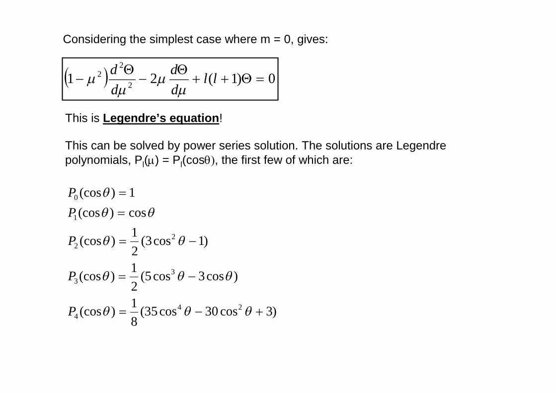
Considering the simplest case where m = 0, gives:
( ) 0)1(21 2
22 =Q++
Q-
Q- ll
dd
dd
mm
mm
This is Legendre’s equation!
This can be solved by power series solution. The solutions are Legendre polynomials, Pl(m) = Pl(cosq), the first few of which are:
)3cos30cos35(81
)(cos
)cos3cos5(21
)(cos
)1cos3(21
)(cos
cos)(cos
1)(cos
244
33
22
1
0
+-=
-=
-=
==
qqq
qqq
qqq
P
P
P
P
P

For the general case, including m ≠ 0, and as long as |m| ≤ l, a solution which remains finite for all values of m is:
)()1()( ||
||2||2 mm
mm lm
mmm
l Pdd
P -=
where Plm(m) is the associated Legendre function.
The associated Legendre function multiplied by the solution to equation 3 for f, and normalised, gives the spherical harmonics which are solutions to Y(q,f) = Q(q)F(f):
fqp
fq imml
ml eP
mlmll
Y )(cos)!()!(
412
),( ×+-+
=

Associated Legendre Functions with argument cosq
qqq
qqq
qqq
qqq
q
333
223
213
203
222
12
202
11
01
00
sin15)(cos
sincos15)(cos
sin)1cos5(23
)(cos
)3cos5(cos21
)(cos
sin3)(cos
cossin3)(cos
)1cos3(21
)(cos
sin)(cos
cos)(cos
1)(cos
-=
=
--=
-=
=
-=
-=
-=
=
=
P
P
P
P
P
P
P
P
P
P

Spherical Harmonics
f
f
f
f
f
f
qp
fq
qqp
fq
qqp
fq
qqp
fq
qp
fq
qqp
fq
qp
fq
qp
fq
qp
fq
pfq
fq
i
i
i
i
i
i
ml
eY
eY
eY
Y
eY
eY
Y
eY
Y
Y
Y
3333
2223
213
303
2222
12
202
11
01
00
sin35
81
),(
cossin2105
41
),(
)1cos5(sin21
81
),(
)cos3cos5(7
41
),(
sin215
41
),(
cossin215
21
),(
)1cos3(5
41
),(
sin23
21
),(
cos3
21
),(
121
),(
),(
-=
=
--=
-=
=
-=
-=
-=
=
=
-
fqp
fq imml
ml eP
mlmll
Y )(cos)!()!(
412
),( ×+-+
=

[ ] )1()(22
2
2
2
22
+=-++ llrVEMr
drdR
Rr
drRd
Rr
h
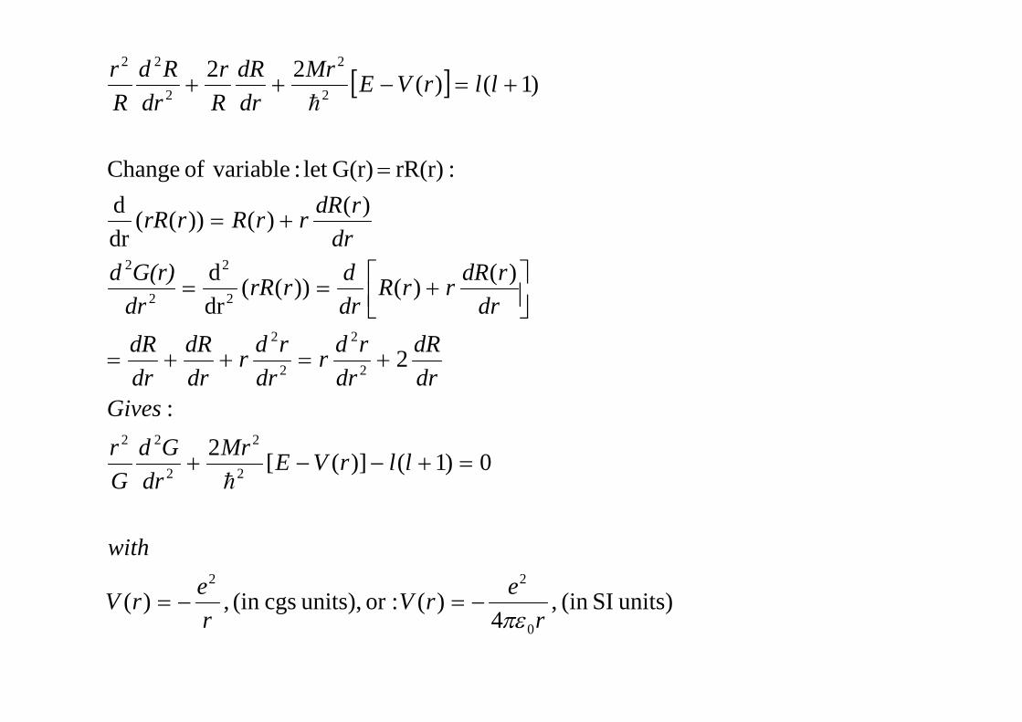
Returning to the radial equation (1):
We introduce the wave number:
22 2)]([ hMrVEk -=
and change the variable to r = kr and replace R by √(p/2kr)R'
2
222
2
2
:rulechain
/ ,
rrrr
rr
r
rr
dRd
kddR
dd
kddR
drd
kdr
Rd
ddR
kdrd
ddR
drdR
krkdrd
=÷÷ø
öççè
æ=÷÷
ø
öççè
æ=
==
==

2
221232325
2
2
2123
22
22
2221
221
243
2221
22
0)1(2
rrp
rrp
rrprp
r
rrprp
r
rpp
rr
rr
r
dRd
dRd
dRd
Rd
Rd
dRd
RddR
RRkr
R
with
llddR
RdRd
R
gives
¢+¢
-¢
-¢=
¢+¢-=
¢=¢=
=+-++
----
--

Substituting in the new expressions for our differential operators into:
( )
RllRdRd
dRd
gives
RlldRd
Rd
RddRd
R
gives
RlldRd
R
dRd
dRd
R
gives
llddR
RdRd
R
¢+-+¢+¢
+¢
¢+-+¢
+¢-¢
+¢
-¢
¢+-+÷÷ø
öççè
æ ¢+¢-+
÷÷ø
öççè
æ ¢+¢
-¢
=+-++
--
---
---
---
21221212
223
21221212
2232121
2122123
2
22123252
22
22
))1((41
))1((243
2)1(
2221
2
22243
0)1(2
rrrr
rr
r
rrr
rrr
rr
rr
rrrr
rprpr
rrp
rrprpr
rr
rr
r

021
have we
41
)1(41
21
21
21
since
))1((41
22
2
22
22
2122
22
-¢÷÷ø
öççè
æ÷øö
çèæ +-+
¢+¢
++=++=÷øö
çèæ +÷øö
çèæ +=÷
øö
çèæ +
¢+-+¢-¢
+¢ -
RldRd
dRd
lllllll
RllRdRd
dRd
gives
rr
rr
r
rrr
rr
r
which is Bessel’s equation!

Solutions to Bessel’s equation:
021
22
2
22 -¢÷
÷ø
öççè
æ÷øö
çèæ +-+
¢+¢
RldRd
dRd r
rr
rr
for half an odd integer, Jl+½, are:
)(2
)()( 21 krJkr
krjrR ll +×==p
which are spherical Bessel functions, the first few of which are:
krkr
krkr
krj
krkr
krj
cos1
sin)(
1)(
sin1
)(
21
0
-=
=
Higher order solutions can be found from the recurrence formula:
)()(12
)( 11 krjkrjkrl
krj lll -+ -+
=

Energy Eigenvalues
Consider the first solution for l = 0:
... 3, 2, 1,
:withby designatedion eigenfuncteach ofenergy kinetic theGives
)]([2
: and umbers, quantum twointroduced have weWhere
2
:zero) still ( issmallest next The
kR
:iscondition thissatisfyingk of aluesmallest v The
radiusnuclear theis R r where
0sin
:requiring condition)(boundary surfacenuclear at the zero bemust This
sin)()(
22
20
10nuc
nuc
0
=
=-=
=
==
=
=
==
v
E
ErVEMk
l
Rk
l
Rk
kRkR
krkr
krjrR
v
vtotvl
nuc
nuc
nuc
nuc
vl
hn
p
p

Evaluation of the model
If we construct a nucleus by assuming that neutrons and protons can populate the same set of energy levels (requiring that no two neutrons or protons can have the same set of quantum numbers and introducing nucleon spin with two possible values: +½ and −½) we predict the first few magic numbers, corresponding to fully occupied energy levels (n): 2, 8 and 20. However, it fails to accurately predict the higher magic numbers given by the shell model.
Our rectangular spherical potential, in which the potential abruptly changes at the nuclear surface, is inaccurate. A more realistic potential would include a more gradual change in potential at the well edge (such as by using the Woods-Saxon potential). We also need to account for fine structure by introducing spin-orbit coupling.
the introduction of spin-orbit coupling accurately predicts all the magic numbers (at least up to 184). The shape of the well (flatness of the well bottom and the steepness of its sides) affects the exact energy levels, but not their order (again we reserve the possibility of differences for very high magic numbers).

2. Modelling the Hydrogen Atom
Using a Coulomb Potential Well
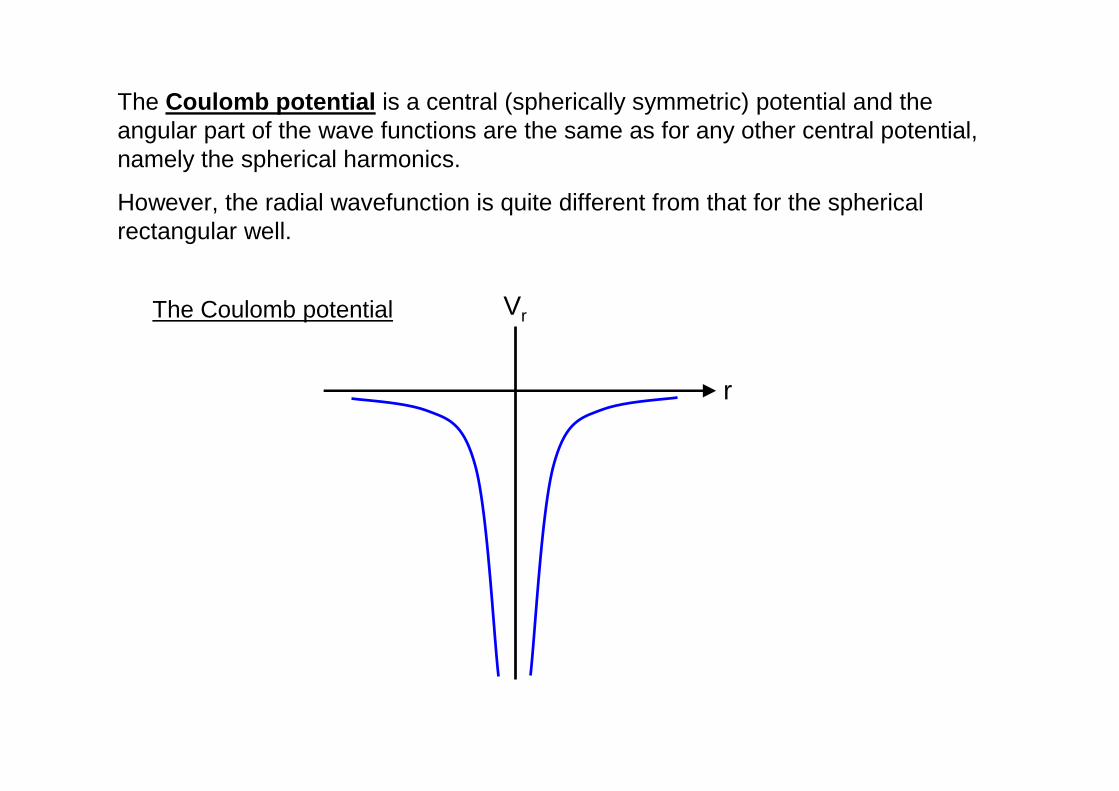
The Coulomb potential is a central (spherically symmetric) potential and the angular part of the wave functions are the same as for any other central potential, namely the spherical harmonics.
However, the radial wavefunction is quite different from that for the spherical rectangular well.
r
VrThe Coulomb potential
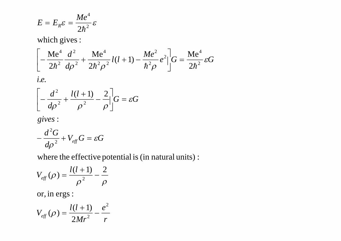
[ ]
units) SI(in ,4
)( :or units), cgs(in ,)(
0)1()]([2
:
2
)()())((
drd
)()())((
drd
:rR(r) G(r)let : variableof Change
)1()(22
0
22
2
2
2
22
2
2
2
2
2
2
2
2
2
2
2
22
re
rVre
rV
with
llrVEMr
drGd
Gr
GivesdrdR
drrd
rdr
rdr
drdR
drdR
drrdR
rrRdrd
rrRdrG(r)d
drrdR
rrRrrR
llrVEMr
drdR
Rr
drRd
Rr
pe-=-=
=+--+
+=++=
úûù
êëé +==
+=
=
+=-++
h
h

rr
e
r
2
2
0
00
2
2
2
2
22
2
22
22
2
ar
have we
radiusBohr theis a where,
:units natural theUsing
2)1(
2
: toequivalent iswhich
02
)1(2
:gives This
Me
EE
ar
EGGre
Mrll
drd
M
GMr
llre
EM
drGd
R
h
hh
hh
==
=
=
=úû
ùêë
é-
++-
=úû
ùêë
é +-++
re
Mrll
V
llV
GGVd
Gd
gives
GGll
dd
ei
GGeMe
lldd
MeEE
eff
eff
eff
R
2
2
2
2
2
22
2
2
42
2
2
22
4
2
2
2
4
2
4
2)1(
)(
:ergsin or,
2)1()(
:units) natural(in is potential effective thewhere
:
2)1(
..
2Me
)1(2Me
2Me
:giveswhich 2
-+
=
-+
=
=+-
=úû
ùêë
é-
++-
=úû
ùêë
é-++-
==
r
rrr
er
errr
errr
ee
hhhh
h

Where the first term on the RHS is the centrifugal potential, l(l+1)/2Mr2, and the second term is the coulomb energy, -e2/r.
Let’s consider limiting cases:
Gebd
Gd
be
b
Gd
Gd
-ε
Gd
Gd
Mrll
for
b
b
er
r
e
r
er
er
r
r
r
r
-==
-=
³=
=+
><
-»
®+
®¥®
-
-
-
22
2
2
b
2
2
2
2
2
ddG
:DE theintoback solution thisngsubstitutiby seen becan As
0,-b where
e~)G(
:isequation thisosolution t acceptableAn
0
:so ,0 so and 0 E states boundFor
:giveswhich
02)1(
and 0energy Coulomb the,

At the other extreme, when r→ 0 we have:
parity. galternatin with states bound theof nature waveheconsider t : thissee To
)1()
:polynomial aby multipliedsolution thisbe toexpected issolution general The
~)G(
:form theof be osolution t expect the weTherefore,
)1()1(
)1(
~)(
:is which ofsolution acceptableAn
)1(
max1
1
12
12
2
1
22
2
å=
-+
-+
+-
+
-=
+=+»
+»
+»
i
oi
ii
ibl
bl
ll
l
l
ceρG(ρ
e
llll
dGd
lddG
G
Gll
dGd
r
rr
rr
rr
rr
rr
rr
r
r

)()1()
:have weso 1/n, bat shortly th see shall We
/1/1max
rr rr feρceρG(ρ nli
oi
ii
inl -+
=
-+ =-=
=
åNow we need to find the values of the coefficients, ci:
2
21112
22
2
11
2
2
122
2
22
2
)1(2
)1(2)1(
)1(dG
:follows as
0)]1(1[2])1[(2
:satisfies )f( shown that becan it then
2)1(2)1(
:satisfies )G( If
rrrr
rrr
rrr
r
rr
rr
r
rerrr
errr
r
rrr
rrr
r
dfd
epddf
epbll
feblbll
dGd
ddf
epfebfeld
flbddf
bld
fd
fell
dGd
GGll
dd
blblbl
blblbl
bl
-+-+-+
-+-+-
-+
+÷÷ø
öççè
æ-
++÷÷
ø
öççè
æ+
+-
+=
+-+=
=+-+-++
÷÷ø
öççè
æ--
+=Þ=ú
û
ùêë
é-
++-
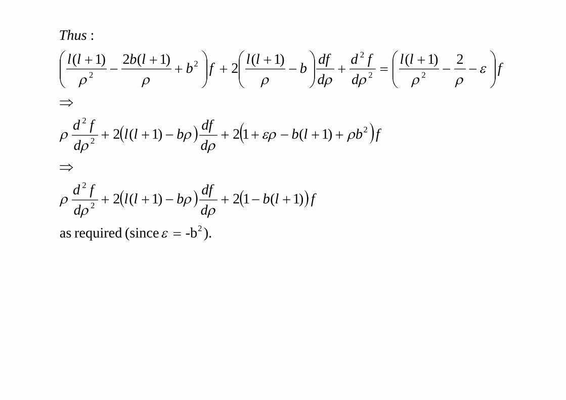
( ) ( )
( ) ( )
).-b (since required as
)1(12)1(2
)1(12)1(2
2)1()1(2
)1(2)1(
:
2
2
2
22
2
22
22
2
=
+-+-++
Þ
++-++-++
Þ
÷÷ø
öççè
æ--
+=+÷÷
ø
öççè
æ-
++÷÷
ø
öççè
æ+
+-
+
e
rr
rr
rerr
rr
r
errrrrrr
flbddf
blld
fd
fblbddf
blld
fd
fll
dfd
ddf
bll
fblbll
Thus
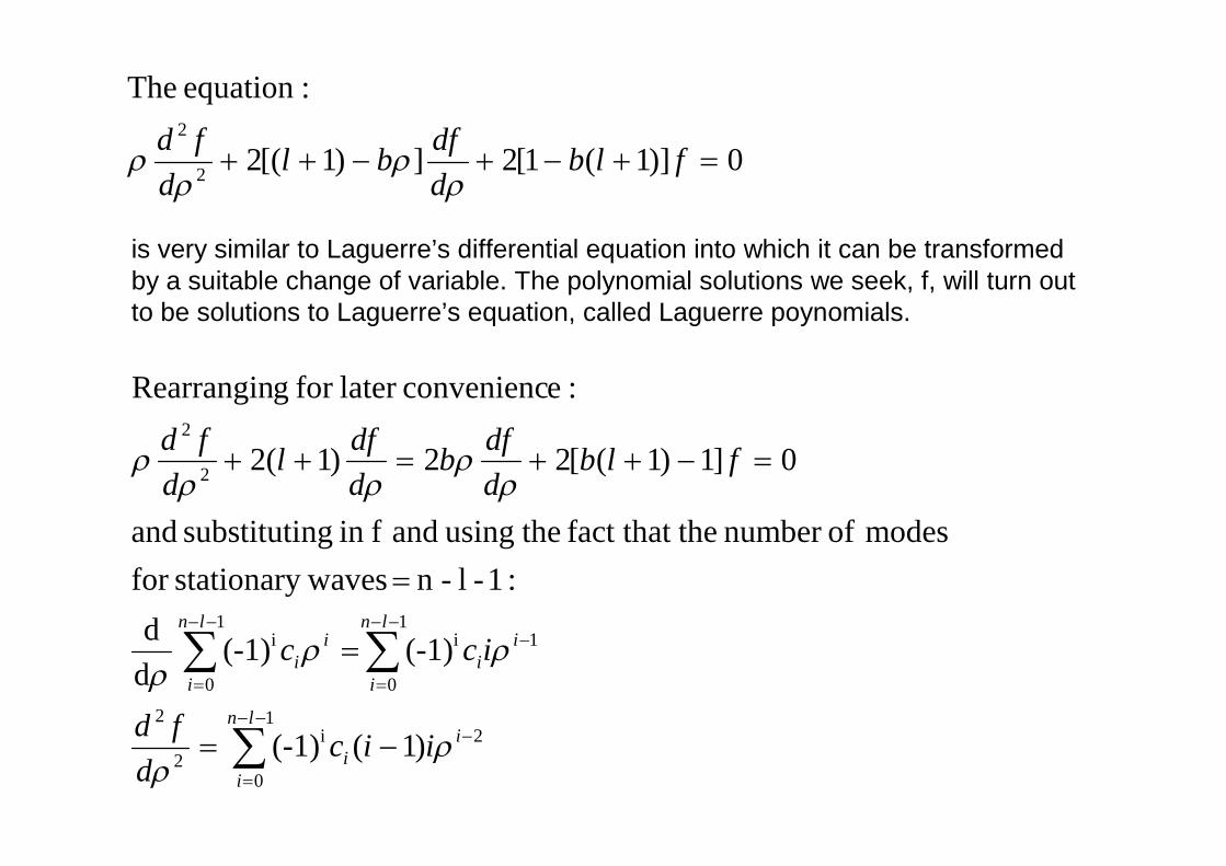
0)]1(1[2])1[(2
:equation The
2
2
=+-+-++ flbddf
bld
fdr
rr
r
is very similar to Laguerre’s differential equation into which it can be transformed by a suitable change of variable. The polynomial solutions we seek, f, will turn out to be solutions to Laguerre’s equation, called Laguerre poynomials.
å
åå--
=
-
--
=
---
=
-=
=
=
=-++=++
1
0
2i2
2
1
0
1i1
0
i
2
2
)1((-1)
(-1)(-1)dd
:1-l-n wavesstationaryfor
modes ofnumber thefact that theusing and fin ngsubstituti and
0]1)1([22)1(2
:econvenienclater for gRearrangin
ln
i
ii
ln
i
ii
ln
i
ii
iicd
fd
icc
flbddf
bddf
ld
fd
rr
rrr
rr
rrr

åå
åå
åååå
--
=
--
=
-
--
=
--
=
-
--
=
--
=
--
=
---
=
-
-++=++-
-++=++-Þ
-++=++-
Þ
1
0
j1
0
1j
1
0
j1
0
1i
1
0
i1
0
i1
0
1i1
0
1j
)]1)1((22[(-1)])1(2)1[((-1)
:
)]1)1((22[(-1)])1(2)1[((-1)
(-1)]1)1([2(-1)2(-1))1(2)1((-1)
ln
i
ii
ln
i
jj
ln
i
ii
ln
i
ii
ln
i
ii
ln
i
ii
ln
i
ii
ln
i
ii
lbbicjljjc
Thus
lbbiciliic
clbicbcliic
rr
rr
rrrr
When j = 1 + 1, we have:
)22)(1()1(2
cc
:tscoefficien for the formula a have weNow
n1b giveswhich
1)]c-1)2(b(l1)-l--[2b(n0
:have we,1 with and zero equal separatelymust each term
)]1)1((22[)]1)(1(2)1([
i
1i
1-l-n
1
iliniln
n-l-i
clbbicilii ii
+++---
=
=++=
=-++-=++++
+
+
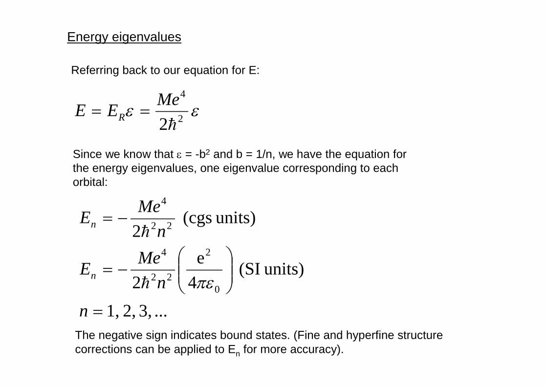
Energy eigenvalues
Referring back to our equation for E:
ee 2
4
2hMe
EE R ==
Since we know that e = -b2 and b = 1/n, we have the equation for the energy eigenvalues, one eigenvalue corresponding to each orbital:
... 3, 2, 1,
units) (SI 4
e2
units) (cgs 2
0
2
22
4
22
4
=
÷÷ø
öççè
æ-=
-=
n
nMe
E
nMe
E
n
n
peh
h
The negative sign indicates bound states. (Fine and hyperfine structure corrections can be applied to En for more accuracy).

Normalisation
We still need to determine the coefficient c0 which will enable us to determine the other coefficients by recursion. To determine c0 we require the integral of the square of the wavefunction = 1, since this is the probability distribution function of the electron and the probability of the electron being somewhere in space = 1.
1a
:1n 0,for
e.g. is, c when normalised is )(f
1)(a
:require we
1sin),(
:normalised YWith
1sin),()(
1sin),,(
/2
0
2
0223
o
0n
/2
0
2223o
0
2
0
2
m
0 0
2
0
22/30
2
2
0 0
2
0
=
==
=
=
=
=
-¥
+
-¥
+
= =
¥
= = =
-
¥
= = =
ò
ò
ò ò
ò ò ò
ò ò ò
dpec
l
dpef
ddY
dddYfea
ddrdrr
nl
l
nnl
l
lm
l
rlmnl
nl
rnlm
r
r
p
q
p
f
p
q
p
f
r
p
q
p
f
r
r
rr
fqqfq
fqrqrfqrr
fqqfqy

on.distributiy probabilit observable obtain the to
ion wavefunct thesquare wesincet unimportan is c ofsign the:Note
2||
:
2||
:obtain We
!r
:integral standard following theUsing
0
2300
30
22
0
01
q
-
¥
+-
=
=
=ò
ac
gives
ac
qdre q
r
aa

0
0
0
0
0
0
3/
2
0
23
032
3/
00
23
031
3/20
2
0
23
030
2/
0
23
021
2/
0
23
020
/23
010
31
527
22
61
31
324
272
32
131
2
21
3
1
21
21
2
12
ar
ar
ar
ar
ar
ar
ear
aR
ear
ar
aR
ear
ar
aR
ear
aR
ear
aR
ea
R
-
-
-
-
-
-
÷÷ø
öççè
æ÷÷ø
öççè
æ=
÷÷ø
öççè
æ-÷÷
ø
öççè
æ÷÷ø
öççè
æ=
÷÷ø
öççè
æ+-÷÷
ø
öççè
æ=
÷÷ø
öççè
æ÷÷ø
öççè
æ=
÷÷ø
öççè
æ-÷÷
ø
öççè
æ=
÷÷ø
öççè
æ=
Some radial wavefunctions, Rnl(r):
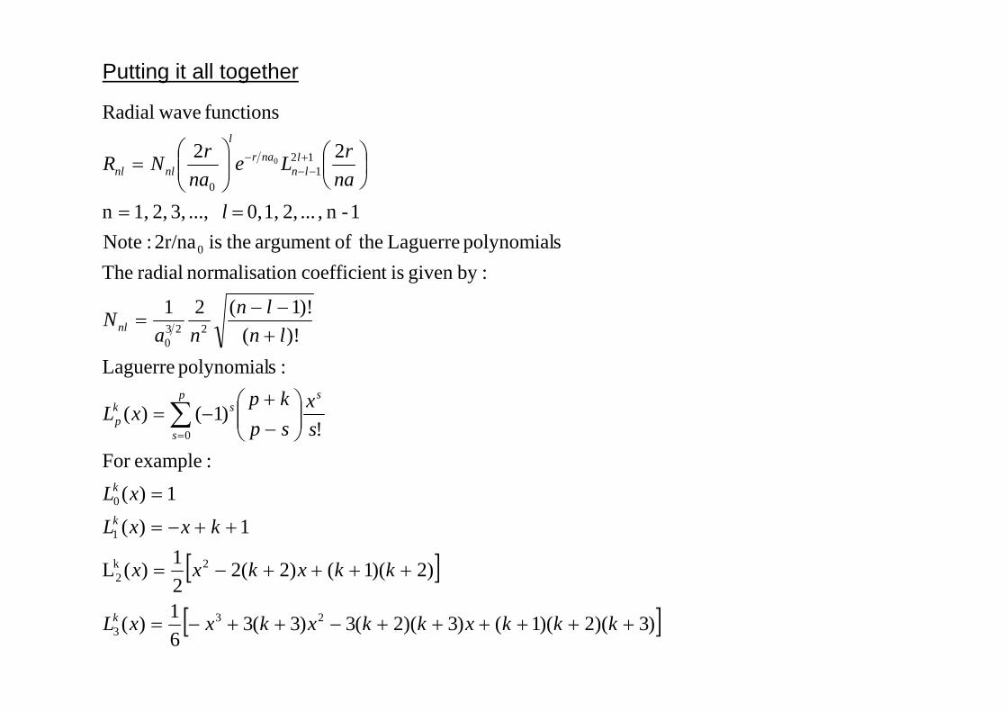
Putting it all together
[ ]
[ ])3)(2)(1()3)(2(3)3(361
)(
)2)(1()2(221
)(L
1)(
1)(
:exampleFor
!)1()(
:spolynomial Laguerre
)!()!1(21
:bygiven ist coefficienion normalisat radial The
spolynomial Laguerre theofargument theis 2r/na :Note
1-n , ... 2, 1, 0, ..., 3, 2, 1,n
22
functions waveRadial
233
2k2
1
0
0
2230
0
121
0
0
++++++-++-=
++++-=
++-=
=
÷÷ø
öççè
æ-+
-=
+--
=
==
÷øö
çèæ
÷÷ø
öççè
æ=
å=
+--
-
kkkxkkxkxxL
kkxkxx
kxxL
xL
sx
sp
kpxL
lnln
naN
l
nar
Lena
rNR
k
k
k
sp
s
skp
nl
lln
nar
l
nlnl

fqqp
y
py
p
iar
ar
eear
ar
aer
Y
)1cos5(sin21
81
2!71
811
)(
:1m with orbital 4f2
2)(
2
1
:orbital 1s
E.g.
24
3
023
0431
230
100
00
0
0
-÷÷ø
öççè
æ-=
=
=
=
-
--