arX

iv:h

ep-t

h/02

0219

9v2

30

Sep

2002

Solutions of the Polchinski ERG equation in theO(N) scalar model

Yu.A. Kubyshin∗

Departament de Matematica Aplicada IV, Universitat Politecnica de Catalunya

C-3, Campus Nord, C. Jordi Girona, 1-3, 08034 Barcelona, Spain

yuri@mat.upc.es

R. Neves and R. Potting

Area Departamental de Fısica, FCT, Universidade do Algarve

Campus de Gambelas, 8000-117 Faro, Portugal

rneves@ualg.pt, rpotting@ualg.pt

Abstract

Solutions of the Polchinski exact renormalization group equation in the scalarO(N) theory are studied. Families of regular solutions are found and their rela-tion with fixed points of the theory is established. Special attention is devotedto the limit N = ∞, where many properties can be analyzed analytically.

Keywords: Exact Renormalization Group; Non-Perturbative Effects.

1 Introduction

The Exact Renormalization Group (ERG) has proven to be a powerful non-perturba-tive method for studies of phenomena in quantum field theories at various scales.It stems from the Wilson renormalization group [1] (see, for example, Ref. [2] for areview) and is, basically, its continuous version adapted to quantum field theory [3]-[6](see Refs. [7]-[11] for reviews). The ERG method allows for general non-perturbativestudies of low-energy effective actions, in particular their flows and fixed points, andis also recognized as a rather powerful calculational framework.

The central object within the ERG approach is the (Wilsonian) effective actionSΛ or the Legendre effective action, which gives an adequate description of the theory

∗On leave of absence from the Institute for Nuclear Physics, Moscow State University, 119899Moscow, Russia.

1

at the scale Λ in terms of renormalized quantities. The action satisfies an equa-tion in functional derivatives which determines completely the renormalization groupevolution of SΛ with the scale. This equation is called the ERG equation.

Various formulations of the ERG have been proposed, the most widely used arethe Wegner-Houghton sharp cutoff equation [3], Polchinski ERG equation for theWilson effective action [5] (see Ref. [12] for detailed derivation and discussion), andequations for the Legendre effective action [13]-[17]. All these equations are essentiallyequivalent, the relation between them was clarified in Refs. [17] and [18]. It turns outthat in practice they are too complicated to be solved exactly. Two well-developednon-perturbative approximate schemes for solving the ERG equations are: (1) trun-cation in the operator content to a finite set of operators [19], and (2) expansion inpowers of space-time derivatives [20]-[22]. Whereas the first scheme is of limited relia-bility [23, 24], the second one, called the derivative expansion, was shown to be quitereliable and accurate enough in finding the fixed points and calculating the criticalexponents [6, 21, 22],[25]-[37]. In particular, the fixed point (FP) corresponding tothe Ising model in three dimensions [6, 22, 26],[35]-[37], and the conformal FPs in twodimensions [27, 32] were calculated using the derivative expansion. The lowest orderof the derivative expansion, O(∂0)-order, also called the local potential approximation(LPA), already gives rather good accuracy in a large variety of problems (see Refs. [6]and [25]). The next-to-leading order (O(∂2)-order) usually improves the results of theleading order and has also been thoroughly studied in the literature (see, for example,Refs. [21, 26, 28] and [31]).

To outline some general features of the ERG approach let us consider the case of ascalar field in d dimensions. A generalization to the fermionic case is straightforward[38]; the gauge invariant formalism is, however, more involved [39]. For a scalar fieldφ the effective interactions within the LPA are restricted to a potential VΛ(φ) of ageneral form and do not include the derivatives. The ERG flow equation reducesto a non-linear second order partial differential equation which symbolically can bewritten as

f(φ, t) = F(f ′′(φ, t), f ′(φ, t), f(φ, t); η, d), (1)

where t = − ln(Λ/Λ0) is the flow parameter, Λ0 is a scale where initial conditions areset,

f(φ, t) = V ′Λ(φ) ≡

∂VΛ(φ)

∂φ,

and η is the anomalous dimension. The prime denotes derivation with respect to thefield φ and the dot denotes derivation with respect to the parameter t. The concreteform of the ERG equation will be given in Sect. 2.

FP solutions f∗(φ) satisfy Eq. (1) with f = 0, i.e. the equation

F(f ′′(φ), f ′(φ), f(φ); η, d) = 0. (2)

For the LPA to be consistent the value of the anomalous dimension in the FP equationmust be set to η∗ = 0. Eq. (2) is supplied with two boundary conditions, usually at

2

φ = 0. Assuming that the theory is symmetric under Z2-transformations φ → −φ,these conditions are often chosen as

f(0) = 0, f ′(0) = γ. (3)

A consistent ERG FP equation always has the trivial solution f∗ = 0. It describes thefree massless theory and is called the Gaussian FP (GFP). For all known formulationsthe ERG equation is stiff and most of its solutions singular at some finite value ofthe field, making them not acceptable from the physical point of view. Moreover, itturns out that only finitely many solutions of Eq. (2) do not end up in a singularity,thus giving massless continuum limits with the prescribed field content [22]. They

correspond to particular values γ = γ(n)∗ , n = 1, 2, . . ..

Let us consider Eq. (2) in a wider mathematical context and study more generalsolutions, namely solutions for arbitrary η. They are parameterized by γ and η(for d fixed), i.e. f = f(φ; γ, η). The dependence of F on η is smooth enough,as a consequence f(φ; γ, η) depends at least continuously on γ and η. It is easy tounderstand that regular solutions correspond to certain points (γ, η) in the space of

parameters which form continuous curves η = ηn(γ). The special values γ(n)∗ , which

were already introduced above, satisfy ηn(γ(n)∗ ) = 0. In what follows, by abuse of

terminology, we will be referring to these regular solutions of Eqs. (2) and (3) witharbitrary η as FP solutions, keeping in mind that physical FPs in the LPA correspondto η = 0. Such curves of regular solutions were first found in Ref. [32].

Obviously, it is useful to know the complete space of solutions of the ERG equationin the leading approximation. There is also a practical reason for studying FP problem(2), (3) with η 6= 0. The FP equations to next-to-leading order, i.e. the equationsobtained with both O(∂0) and O(∂2) terms in S taken into account, form a systemof coupled nonlinear differential equations. They are stiff and solving them require asimultaneous fine tuning of η and γ. This makes the direct integration of the systema hard task, and one of the ways to solve it is to use an iterative numerical procedure[26]. In some cases, as for example for d = 3, one can perform such iterations startingwith a solution of the first order FP equation with η = 0, i.e. with a physical FP.1

However, for d = 2 this is no longer possible. It turns out that due to the natureof the problem only periodic or singular solutions, neither of which is a physical FP,exist for η = 0 [27, 32] (see Sect. 2 for details). For this reason one needs leadingorder FP solutions with η 6= 0 as initial solutions to start the iteration procedure.

In the present article we study solutions of the Polchinski ERG equation in O(N)scalar field theories. Though much research on the structure of the space of solutionshas been already done, we feel that some questions remain unanswered. Namely, inall previous articles the condition of regularity was imposed in the course of numericalintegration of the equation (see Refs. [22, 23, 26] and [29] for algorithms). No ”an-alytical” understanding of how this condition works and how it gives rise to critical

1This solution is the Wilson-Fischer FP for d = 3.

3

curves ηn(γ) was gained. Also, the relation between the curves and the asymptotics ofthe solutions f(φ) for large φ remains obscure. To explain this last issue we note thatsolutions of the Polchinski ERG equation in the LPA have, for large φ, the asymptoticform [26]

f(φ; γ, η) ∼(

1− η

2

)

φ+ D(η, γ)φ−∆−

∆+ + · · · , (4)

where we introduced

∆± = 1± d

2− η

2. (5)

The coefficient D(η, γ) in expansion (4) cannot be derived from the asymptotic anal-ysis of Eq. (2) alone, without solving the FP equation. Fixing D is equivalent tosetting the boundary conditions at φ = ∞, and only a countable number of values ofthis coefficient correspond to FP solutions. The values depend on γ and ηn in someintrinsic way. In the present article we will address these and other related issues.

We found it convenient to study them in the context of O(N) scalar theories. Thereason is that for N = ∞ a general solution of the lowest order ERG flow equationis known analytically though indirectly [29, 40, 41]. Namely, the inverse functionφ = φ(f, t) can be obtained in a closed analytical form. This will be enough forour purpose. We will study various properties of the corresponding FP solutions forN = ∞ and relate them to the analogous properties of FP solutions for finite N ,where only numerical or approximate analytical results are available. In particular,we will analyze the appearance of the critical curves ηn(γ) of regular solutions forN = ∞ and see how they change for finite N .

We would like to note that O(N) scalar models (also called spherical models) areinteresting on their own [42]. They play an important role in the description of phasetransitions. In particular, N = 4 is relevant for the QCD phase transition [2, 14, 43].These models were also studied within the ERG using the 1/N -expansion [44] (seeRefs. [10] and [30] for other studies and references therein).

The plan of the article is the following. In Sect. 2 we introduce basic notations anddiscuss the Polchinski ERG equation in the O(N) scalar model for finite N . Sect. 3is devoted to the Polchinski ERG equation in the limit N = ∞. We formulate thecondition of regularity of solutions, find regular solutions and study their propertiesin detail. The appearance of critical curves η = ηn(γ) is analyzed. In Sect. 4 weanalyze the behavior of the critical curves for finite N and show that they match theN = ∞ case. Sect. 5 contains some discussion and concluding remarks.

2 O(N) Polchinski ERG equation

In this article we consider a general O(N)-symmetric scalar field theory in d-dimen-sional Euclidean space.

4

Let us denote the field components by φa(x), a = 1, 2, . . . , N and assume that theWilson effective action at the scale Λ is of the following general form:

SΛ[φ] =1

2

∫

ddp

(2π)dφp ·M(p2,Λ) · φ−p + Sint,Λ[φ]. (6)

Here φap denotes the field in the momentum representation, i.e. the Fourier transform

of φa(x). In fact the field depends on the scale Λ as well, i.e. φap = φa(p; Λ). The dots

in Eq. (6) stand for the contraction over indices of O(N). The inverse propagator is

Mab(p2,Λ) = δab

1

P (p2,Λ),

P (p2,Λ) =K(p2/Λ2)

p2,

where K(p2/Λ2) is a cutoff function (also called a regulating function or simply aregulator) [5, 12]. It has to satisfy the following two requirements: (1) K(0) = 1,and (2) K(z) → 0 as z → ∞ fast enough. The second property guarantees thatcontributions of high momentum modes are suppressed. In some studies on the ERGa sharp cutoff function, defined by K(z) = 1 for 0 ≤ z ≤ 1 and K(z) = 0 for z > 1,was used [3, 6]. This choice corresponds to integrating out modes with p2 > Λ2

exactly. In the present article we assume that K(z) is a smooth enough function, sothat higher momentum modes are integrated out effectively. The term Sint,Λ[φ] is theinteraction term. In general it contains all possible O(N)-invariant interactions.

2.1 Polchinski ERG equation for arbitrary N

The central idea of the ERG approach is essentially the following: under a change ofthe scale Λ the Wilson effective action changes in such a way so that the generatingfunctional of the theory and, therefore, the Green functions remain unchanged [3, 5].This requirement gives rise to an equation on SΛ[φ] which is called an ERG flowequation. One of the most widely used versions is the Polchinski equation:

Λd

dΛS[ϕ; Λ] =

1

2

∫

ddp

(2π)dΛdP (p2,Λ)

dΛ

[

δS

δϕ−p· δS

δϕp

− 1

NTr

(

δ2S

δϕ−pδϕp

)

− 2P−1(p2,Λ)ϕp ·δS

δϕp

]

, (7)

where we introduced ϕap = φa

p/√N and S = S[ϕ; Λ] = (1/N)SΛ[φ], the notations

which will be convenient in the N → ∞ limit. This equation for N = 1 was firstderived and discussed in Ref. [5], for N > 1 it was studied in Ref. [29].

The structure of Eq. (7) becomes more transparent if it is rewritten in terms of thedimensionless momentum p = p/Λ and the dimensionless field variable ϕa

p = Λ1+d/2ϕap.

5

We also introduce the renormalization group flow parameter t = − ln(Λ/Λ0), whereΛ0 is some fixed ultraviolet reference scale. When expanded in powers of ϕa

p a generalaction of interaction has the form

Sint[ϕ; t] =∞∑

k=1

∫

ddp1 . . . ddp2k

(2π)d(2k−1)sn;a1,...a2k(p1, . . . , p2k; t)

× ϕa1p1ϕa2p2. . . ϕa2k

p2kδ(d)(p1 + . . .+ p2k). (8)

Note that the terms of the expansion contain only an even number of fields and areO(N)-invariant. The Polchinski ERG equation, Eq. (7), becomes

∂S

∂t=

∫

ddp

(2π)dK ′(p2)

[

δS

δϕ−p· δS

δϕp− 1

NTr

(

δ2S

δϕ−pδϕp

)]

+ Sd+∫

ddp

(2π)d

[

1− d

2− η(t)

2− 2p2

K ′(p2)

K(p2)

]

ϕp ·δS

δϕp

−∫

ddp

(2π)dϕp · p ·

∂′

∂p

δS

δϕp. (9)

The partial derivative in the l.h.s. acts on the t-dependent coefficient functionssn;a1,...a2k in Eq. (8) and does not act on ϕa

p. The scale dependence of the field ϕap is

determined by

dϕap

dt=

[

−1− d

2+

η

2

]

ϕap,

where η is the anomalous dimension, and has already been taken into account in Eq.(9) by adding the rescaling terms (the second line in Eq. (9)). The prime in themomentum derivative in the last term in the r.h.s. means that it does not act on theδ-function of the energy-momentum conservation (see Eq. (8)).

Being supplied with an initial condition S[ϕ; t = 0] = S0[ϕ] at t = 0 (or Λ = Λ0),where S0[ϕ] is some given functional, Eq. (9) determines the flow of the effective actionand allows to calculate, at least in principle, the action and physical characteristicsof the theory at low energies, when Λ → 0 (or t → +∞). The limit Λ0 → ∞, whenthe cutoff scale Λ0 is removed, is called the continuum limit and corresponds to therenormalized theory.

2.2 Leading order approximation

As was mentioned already in the Introduction, to find solutions of the ERG equationin concrete calculations various approximate (but non-perturbative) techniques areused. A reliable and efficient one is the derivative expansion. In the coordinate

6

representation it corresponds to the following expansion of the action of interactionin powers of derivatives:

Sint[ϕ; t] =∫

ddx

V(

ϕ2; t)

+ Z(

ϕ2; t)

(

∂ϕ(x)

∂xµ

)2

+ W(

ϕ2; t)

(

ϕ(x) · ∂ϕ(x)∂xµ

)2

+ . . .

,

where the potentials V , Z and W do not contain derivatives of the field. We also tookinto account that these functions depend on the field only through the O(N)-invariantcombination ϕ2 = ϕ(x) · ϕ(x) ≡ ϕa(x)ϕa(x). Restricting the action to the first termgives the leading-order of the derivative expansion, the LPA. In this approximationthe Polchinski ERG equation reduces to a partial differential equation for the functionV (z2; t), where we denoted ϕ2 = z2. Introducing the notation f(z, t) ≡ ∂

∂zV (z2; t),

one can write the equation as

f =1

Nf ′′ − 2ff ′ +

[(

1− 1

N

)

1

z+∆−z

]

f ′ +[

∆+ −(

1− 1

N

)

1

z2

]

f, (10)

where the dot and prime denote the derivative with respect to the flow parameter tand variable z respectively and, as before,

∆± = 1± d

2− η

2

(see Eq. (5)). FP solutions f(z) are solutions of Eq. (10) with the property f = 0,i.e. they satisfy the equation

1

Nf ′′ − 2ff ′ +

[(

1− 1

N

)

1

z+∆−z

]

f ′ +[

∆+ −(

1− 1

N

)

1

z2

]

f = 0. (11)

Note that η is constant here.In this paper we will assume that the potential V (z2) is analytic in z2 at z2 = 0, i.e.

V (0) is finite and its expansion at z = 0 is convergent and contains only non-negativeinteger powers of z2 = φ2. This assumption is fulfilled in most of scalar models and,therefore, does not add new essential restrictions in field theory applications of theERG. Correspondingly, the expansion of f(z) at z = 0 includes only odd powers ofz. To have a unique FP solution we must add two conditions on f(z). In field theoryproblems it is natural to impose them at z = 0 in the form

f(z)|z=0 = 0, f ′(z)|z=0 = γ. (12)

For purely historical reasons these conditions are called initial conditions. The firstcondition is a consequence of the O(N)-symmetry of the potential V (ϕ2). The pa-rameter γ plays the role of the square of the mass of the field.

7

For further studies it is convenient to define a new variable y and a new functionu(y, t) instead of z and f(z, t) in the following way:

z =√

2y, (13)

f(z, t) =

√

y

2u(y, t). (14)

Note that these formulas define u(y, t) on the semi-axes y > 0 only. In terms of y andu(y, t) Eq. (10) becomes

u(y, t) =2y

Nu′′yy − 2yuu′

y − u2 +(

1 +2

N+ 2y∆−

)

u′y + su, (15)

where we introduced the notation

s ≡ ∆+ +∆− = 2− η. (16)

The prime in Eq. (15) denotes the derivative with respect to y. The FP equationnow reads

2y

Nu′′yy − 2yuu′

y − u2 +(

1 +2

N+ 2y∆−

)

u′y + su = 0. (17)

Let us rewrite initial conditions (12) in terms of u(y). Using relations (13), (14) itis easy to check that the condition f(0) = 0 together with the assumption about thebehavior of f(z) at z = 0 are equivalent to the requirement that u(y) is analytic aty = 0, i.e. u(0) is finite and its expansion at y = 0 is convergent and contains onlynon-negative integer powers of y. Therefore, from now on we will be interested onlyin solutions of Eq. (17) which are analytic at y = 0. The second initial condition in(12) transforms to

u(y)|y=0 = 2γ. (18)

Using the analyticity of u(y) the value of u′(y) at the origin can be calculated fromthe FP equation (17):

u′(y)|y=0 =2γ(2γ − s)

1 + 2N

.

In fact, to be physical solutions functions f(z) or u(y) must satisfy even strongerrequirements. Recall that f(z) is the derivative of the effective potential V withrespect to the field variable. In field theory applications one is interested in solutionssuch that V (ϕ2) and its derivatives are finite and do not have singularities for allfinite values of the field variable. This means that f(z) does not have singularitiesfor finite z or, equivalently, u(y) does not have singularities for finite y ≥ 0. Suchsolutions will be called regular solutions.

8

From Eqs. (11) and (12), or, equivalently, from Eqs. (17) and (18), one can seethat for a given d a FP solution is completely determined by the values of γ and η.Correspondingly, any solution of the FP problem can be represented by a point (γ, η)in the parameter space.

One comment is in order. Since the potentials Z andW are not taken into accountin the LPA, the kinetic term in the effective action, which contains two derivativesof the field, matches ERG equation (9) for η = 0 only. Regular solutions of Eqs.(11), (17) with η = 0 will be called physical FPs. As we have already explained inthe Introduction, we will relax this condition and study a wider class of FP solutionswith η 6= 0. To summarize, in the present article we will study solutions u(y) of Eq.(17) with arbitrary η, both regular and non-regular, which satisfy condition (18) andare analytic at y = 0.

The asymptotics of a solution u(y) for large y can be obtained from ERG equation(17) by a straightforward calculation. Namely, one writes a general expression for theexpansion of u(y) as a series in decreasing powers of y and fixes the coefficients andthe exponents from Eq. (17). One gets

u(y) = s−Dyβ − αD2

s(2− α)y2β − D3

s2α(α + 1)

(2− α)2y3β −D

1 + 2Nβ

s(2− α)2yβ−1 + · · · , (19)

where

α =2∆−

s=

2∆−

∆+ +∆−, β = − 1

2− α= − s

2∆+.

As was already mentioned in the Introduction, this technique does not allow to fixthe constant D = D(γ, η). Expansion (19) is, of course, in a full correspondence withasymptotic formula (4) with

D = 2− 1

2

(

∆−

∆+−1

)

D.

The FP equation has two trivial solutions. The first one is obtained for γ = 0 andis equal to f = 0. This is the GFP describing the free massless theory. It correspondsto the line γ = 0 on the (γ, η)-plane. The second solution is obtained for γ = s/2and is given by the linear function f(z) = sz/2, where s is defined in Eq. (16). Thesesolutions, termed high temperature FPs or infinite mass GFPs, are described by thestraight line η = 2− 2γ on the (γ, η)-plane. For the sake of brevity we will call themtrivial FPs (TFP). As one can easily see from Eqs. (14) and (13), these solutionscorrespond to u = 0 and u = s respectively.

2.3 N = 1 case

Before starting the analysis of FP solutions in the O(N) model for arbitrary N it isinstructive to consider the N = 1 model. In this case the O(N)-symmetry reduces to

9

the Z2-symmetry under the reflection φ → −φ. The leading order Polchinski ERGequation (11) with initial condition (12) becomes the familiar FP problem (see [26])

f ′′(z)− 2f(z)f ′(z) + ∆−zf ′(z) + ∆+f(z) = 0, (20)

f(0) = 0, f ′(0) = γ. (21)

For ∆− = 0 or ∆+ = 0 this equation can be integrated analytically. Let us analyzethe case ∆− = 0 first. With this condition, which implies ∆+ = d, Eqs. (20) and (21)become

f ′′(z)− 2f(z)f ′(z) + df(z) = 0, f(0) = 0, f ′(0) = γ. (22)

Denoting g = f ′ one can rewrite Eq. (22) as a first order differential equation forg(f):

gdg

df= f [2g(f)− d] , g(f)|f=0 = γ. (23)

If γ < d/2 solutions to problem (23) are given by the following periodic trajectoriesin the phase space (f, f ′) = (f, g):

f 2 = g − γ +d

2ln

(

d/2− g

d/2− γ

)

.

In particular, for |γ| ≪ d the trajectories are given approximately by ellipses

d · f 2 + g2 = γ2.

This family of regular solutions corresponds to the straight line η = 2 − d for allγ < d/2 on the (γ, η)-plane. Note that for d = 2 they are solutions with η = 0.

If γ ≥ d/2 the trajectories in the phase space are unbounded. They describesolutions f(z) which are singular at some finite value of z.

Let us consider now the case ∆+ = 0, i.e. η = 2 + d. Eqs. (20) and (21) become

f ′′(z)− 2f(z)f ′(z)− dzf ′(z) = 0, f(0) = 0, f ′(0) = γ. (24)

Solutions of this problem can be obtained from solutions of Eq. (22) with γ substitutedby γ + d/2. Indeed, let function h(z) be a solution of

h′′(z)− 2h(z)h′(z) + dh(z) = 0, h(0) = 0, h′(0) = γ +d

2

(cf. (20)). As one can easily check, then f(z) = h(z)− (d/2)z is a solution of problem(24).

10

In a general case solutions of (20), (21) can be found only numerically. A genericsolution f(z) or its derivative end up with a singularity at a finite point z = z0, i.e.,is not regular. A natural method for searching regular solutions is to fine tune η andγ in such a way that the position of singularity z0 = z0(γ, η) → ∞. A realizationof this recipe in a practical computation is to pick a solution for which z0 shows atendency to diverge [22, 26].

First we studied numerically solutions of the FP problem, Eqs. (20) and (21), ford = 2, in a wide range of values of γ, η. We found that for η = 0 and any γ < 1there is a periodic solution. This is in accordance with our analytic result for ∆− = 0above (note that for d = 2 ∆− = −η/2).

-0.6 -0.4 -0.2 0 0.2 0.4 0.6γ

0

0.2

0.4

0.6

0.8

1

η

d=2

-0.6 -0.4 -0.2 0 0.2 0.4 0.6γ

-0.8

-0.6

-0.4

-0.2

0

0.2

0.4

η

d=3

Figure 1: Non-trivial FP curves for d = 2 and d = 3. Only the first 7 curves areshown.

For 0 < η ≤ 1 and η < 2 − 2γ the parameter γ can be fine tuned to a certainvalue so that a non-trivial regular FP solution exists. The set of such values (γ, η)form an infinite discrete series of curves ηn(γ) (n = 1, 2, 3, . . .) shown in Fig. 1. Atγ = 0 ηn(0) = 2/(n+ 1). The curves accumulate at the line η = 0 as n → ∞.

There are general grounds to expect the existence of the curves ηn(γ) whose points(γ, ηn(γ)) correspond to regular FP solutions [32]. Indeed, let us suppose that for somevalue (γ′, η′) there exists a regular solution. This means that the singularity of thissolution is situated at z0(γ

′, η′) = ∞. Consider now another value η′′ sufficiently closeto η′. Assuming that the function z0(γ, η) is continuous in the vicinity of (γ′, η′) itis clear that there exists the value γ′′ such that again z0(γ

′′, η′′) = ∞. Consequently,there is a curve η(γ) passing through the point (γ′, η′) in the parameter space. Thecurve is defined by the equation z0(γ, η) = ∞.

We found that when moving along a given curve ηn(γ) the shape of the corre-sponding solution qualitatively remains the same. When passing from one curve toanother the shape of the solution changes significantly following the same regularpattern as the one obtained by T.R. Morris within the Legendre ERG equation [27].

11

Since all the curves ηn(γ) are situated in the η > 0 half-plane, their presence is asignal of the existence of an infinite number of non-trivial FPs in two-dimensionalscalar theories. This expectation turns out to be true. As it was shown in Refs. [27]and [32] by studying the next-to-leading ERG equations, they do correspond to theminimal unitary series of p(p+ 1) (p = 3, 4, . . .) conformal models.

For d = 3 we found periodic solutions corresponding to η = −1. Again, this isin accordance with our analytic results for ∆− = 0 because for d = 3 the condition∆− = 0 leads to η = −1. We also found an infinite number of critical curves η = ηn(γ),n = 1, 2, . . ., corresponding to non-trivial regular FP solutions of Eqs. (20) and (21).They are plotted in Fig. 1. The curves accumulate at the line η = −1 as n → ∞. Atγ = 0 ηn(0) = (2− n)/(n+1). The curve η1(γ) crosses the γ-axis at γ∗ = −0.229 . . ..The value of γ coincides with the one for which a non-trivial physical FP was foundin the LPA of the Polchinski equation [26]. This is the well-known Wilson-FischerFP analyzed in numerous previous studies (see [6],[22]-[24], [31], [35]-[37]. It belongsto the Ising model universality class. The rest of the curves are situated between thehorizontal lines η = 0 and η = −1 (except for the value of η2(γ) at γ = 0: η2(0) = 0,the GFP). This suggests that for d = 3 there is only one non-trivial physical FP,namely the one associated with the curve η1(γ).

3 N = ∞ Polchinski ERG equation

In this section we will study solutions of the leading order Polchinski ERG equationfor N = ∞. In this limit many features of the solutions can be described analytically,and we are going to take advantage of this. Our aim is to study the η(γ) curves ofregular FP solutions for N = ∞. We expect them to be certain smooth deformationsof the analogous curves for finite N , therefore the analysis of the N = ∞ case willhelp us to understand the features of the η(γ) curves for finite N .

3.1 Equation and general solution

In the limit N → ∞ the Polchinski flow equation, Eq. (15), simplifies considerablyand becomes

u(y, t) = −2yuu′y − u2 +

(

1 + 2y∆−)

u′y + su (25)

for −∞ < t < ∞ and y ≥ 0 (see Eq. (13)).The FP equation for u(y) follows from Eqs. (17) and (18), and is given by

− 2yuu′y − u2 +

(

1 + 2y∆−)

u′y + su = 0, (26)

u(y)|y=0 = 2γ. (27)

12

As in the case of finite N , Eq. (26) is solved by the GFP u(y) = 0 and by the TFPu(y) = s.

Let us consider solutions of flow equation (25) first. As was pointed out in Ref. [29],it can be solved analytically for the inverse function y(u, t). Indeed, from Eq. (25)one obtains the following flow equation for y(u, t):

y(u, t) = (u− s)uy′u − 2(

∆− − u)

y − 1. (28)

Its general solution is equal to [29]

y(u, t) =1

(s− u)2−αuαF(

s− u

uest)

+ y(u), (29)

where

α = 2∆−/s, (30)

F is an arbitrary function and y(u) satisfies the inverse FP equation, i.e. Eq. (28)with y = 0, and the corresponding initial condition:

(u− s)uy′u − 2(

∆− − u)

y(u)− 1 = 0, (31)

y(2γ) = 0. (32)

The FP equation, of course, can also be obtained directly by inverting Eq. (26).Condition (32) follows from (27).

Eq. (31) can be solved analytically [29]. Its general solution is given by

y(u) =1

(s− u)2−αuα

[

−uα(s− u)1−α

α+

α− 1

α

∫ u

0

(

s− z

z

)−α

dz − C

]

. (33)

Note that it is consistent with general solution (29) with the function F taken to beconstant, F = −C.

The form of the solution is not unique and integrating by parts one can bring it toanother one. Possible divergences of the integral in Eq. (33) can be absorbed in theintegration constant C. Equivalently, one can choose the lower limit to be u0 6= 0, inthis case C becomes u0-dependent.

It is important to bear in mind that a solution u(y) may not be monotonous and,therefore, not invertible on the whole semi-axis y ≥ 0. As an example let us considerthe case in which u(y) is monotonically decreasing in a subinterval 0 ≤ y ≤ y# andmonotonically increasing in the infinite interval y# ≤ y < ∞. One has u(0) > u(y#)and u(∞) > u(y#). In each of these regions u(y) is invertible, let us denote thecorresponding inverse functions as y(<)(u) and y(>)(u) respectively. The former isdefined for u# ≤ u ≤ u(0), where u# ≡ u(y#), the latter for u# ≤ u < u(∞). Theyhave to satisfy the following matching condition:

13

y(<)(u#) = y(>)(u#). (34)

Hence, there are two branches of y(u), y(<)(u) and y(>)(u), such that their inversefunctions form the solution u(y) for 0 ≤ y < ∞. Note that initial conditions (27) and(32) imply that y(<)(u(0)) = y(<)(2γ) = 0. This equality fixes the integration constantC in formula (33) for the y(<)(u) branch. The analogous constant in the expression forthe y(>)(u) branch is fixed by the matching condition, Eq. (34). Concrete exampleswill be considered in Sect. 3.3.

To conclude this discussion we stress once more that Eq. (33) gives the exactgeneral solution of the Polchinski FP equation, Eq. (26), in the LPA in terms of theinverse function y(u). The constant C is fixed either by initial condition (32) or by amatching condition similar to (34).

The parameter α, defined by (30), turns out to be very convenient in the analysisof FP solutions. The anomalous dimension η and the parameter s are expressed interms of α as follows:

η = 2− d

1− α, s =

d

1− α. (35)

There are different types of solutions for different intervals of values of α. The intervalwhich is most interesting for physical applications is

− 1 < α < 0. (36)

It corresponds to the range 2 − d < η < (4 − d)/2. From now on we will only beconsidering interval (36) of values of α. The form of the solution, given by Eq. (33),is adequate to this interval.

The asymptotics of the solution u(y) for large y is given by the N → ∞ limit ofEq. (19). In the case in hand it can also be found from exact formula (33). For thiswe first calculate the asymptotic behavior of the function y(u) as u → s and theninvert the asymptotic formula. This procedure not only reproduces formula (19), butalso allows to determine the constant D. One obtains

D =

[

sα

C − πdsinπα

]− s

2∆+

.

Now we turn to the analysis of the expression for the derivative of the solutionu(y) following from Eq. (26):

u′y =

u(s− u)

2uy − (1 + 2y∆−). (37)

The denominator is zero if 2yu = (1 + 2y∆−). Let us introduce the function

using(y) =1 + 2y∆−

2y. (38)

14

For α satisfying (36) we have s > 0 and ∆− < 0. It follows that a general solution u(y)with initial condition u(0) = 2γ (see (27)) and asymptotics limy→∞ u(y) = s (fromEq. (19)) necessarily crosses the curve of potential singularities using(y) at some pointy = ysing. In other words, there always exists at least one point ysing > 0 such thatu(ysing) = using(ysing). Let us denote this value of u as u0,

u0 ≡ u(ysing) =1 + 2ysing∆

−

2ysing.

Since in general u0 6= 0, u0 6= s the derivative of the solution does not exist at thispoint and the solution is singular.2

Note that this picture has an equivalent description in terms of the inverse functiony(u). Its derivative is obtained from Eq. (31),

y′u =1 + 2(∆− − u)y

u(u− s).

So the line of potential singularities is

ysing(u) =1

2(u−∆−), (39)

the inverse function of using(y).A general solution y(u) always intersects this curve at some point, namely at

u = u0 (see Fig. 2). Note that in general there may be a few points of intersection.If u0 6= 0, u0 6= s the derivative y′u vanishes, the derivative u′

y does not exist, and thesolution is singular.

The analysis of relation (37) shows that a general solution has the following be-havior near the point of singularity:

u(y) = u0 + A√

y − ysing + b(y − ysing) + c(y − ysing)3/2 + · · · . (40)

The coefficients are determined from Eq. (37) and are equal to

A = ±√

√

√

√

u0(s− u0)

ysing, b =

s+∆− − 3u0

3ysing, etc.

Using these expressions one can easily see that the solution is indeed non-analyticand the derivative does not exist at y = ysing:

u′(y) =A

2√y − ysing

+ b+ · · · . (41)

By inverting a general solution, Eq. (40), one gets the following expansion for y(u) inthe vicinity of u = u0:

2This observation was made in Ref. [29].

15

-0.2 -0.1 0 0.1 0.2u

0.5

1

1.5

2

2.5

y

d=3

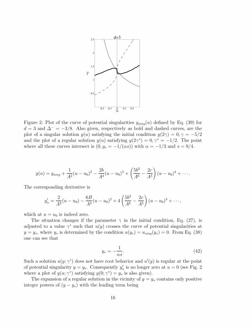
Figure 2: Plot of the curve of potential singularities ysing(u) defined by Eq. (39) ford = 3 and ∆− = −3/8. Also given, respectively as bold and dashed curves, are theplot of a singular solution y(u) satisfying the initial condition y(2γ) = 0, γ = −5/2and the plot of a regular solution y(u) satisfying y(2γ∗) = 0, γ∗ = −1/2. The pointwhere all these curves intersect is (0, y∗ = −1/(αs)) with α = −1/3 and s = 9/4.

y(u) = ysing +1

A2(u− u0)

2 − 2b

A4(u− u0)

3 +

(

5b2

A6− 2c

A5

)

(u− u0)4 + · · · .

The corresponding derivative is

y′u =2

A2(u− u0)−

6B

A4(u− u0)

2 + 4

(

5b2

A6− 2c

A5

)

(u− u0)3 + · · · ,

which at u = u0 is indeed zero.The situation changes if the parameter γ in the initial condition, Eq. (27), is

adjusted to a value γ∗ such that u(y) crosses the curve of potential singularities aty = y∗, where y∗ is determined by the condition u(y∗) = using(y∗) = 0. From Eq. (38)one can see that

y∗ = − 1

αs. (42)

Such a solution u(y; γ∗) does not have root behavior and u′(y) is regular at the pointof potential singularity y = y∗. Consequently y′u is no longer zero at u = 0 (see Fig. 2where a plot of y(u; γ∗) satisfying y(0; γ∗) = y∗ is also given).

The expansion of a regular solution in the vicinity of y = y∗ contains only positiveinteger powers of (y − y∗) with the leading term being

16

u(y) = bn(y − y∗)n + higher powers of (y − y∗). (43)

It is the leading power n which defines the type of the solution. It turns out thatthere are two qualitatively different classes of regular solutions: (1) with n = 1, and(2) with n ≥ 2.

For n = 1 the expansion at y = y∗ is given by

u(y) = b1(y − y∗) + b2(y − y∗)2 + b3(y − y∗)

3 + · · · , (44)

b1 = −s2α(α+ 1)

2, b2 = −3s3α2(α+ 1)2

4(α+ 2). (45)

For n ≥ 2, as one can find out using ERG FP equation (26) or Eq. (37), the behaviorof the solution is more complicated:

u(y) = bn(y − y∗)n + c2n(y − y∗)

2n−1 + b2n(y − y∗)2n (46)

+ d3n(y − y∗)3n−2 + c3n(y − y∗)

3n−1 + · · · .

For such a function to satisfy the equation the parameter α must be fixed to the valueα = −1/n. This amounts to η = 2 − dn/(n + 1), s = dn/(n + 1), etc. However, thecoefficient bn is not fixed by the equation and remains a free parameter. In otherwords, there is a regular solution for any value of bn. The rest of the coefficients areexpressed in terms of bn. For example,

c2n = − 2n3

s2(n− 1)b2n, b2n = −2n + 1

sb2n, etc.

Note that for n = 2 the terms proportional to (y − y∗)2n and to (y − y∗)

3n−2 give thesame power of (y − y∗)

4 so that expansion (46) is of the form

u(y) = b2(y − y∗)2 + c4(y − y∗)

3 + (b4 + d6)(y − y∗)4 + · · · .

Let us analyze the expansion of the corresponding inverse functions y(u) aroundy∗. Consider the two classes of regular solutions.

(i) For the solution u(y) with n = 1 the inverse function y(u) has the followingbehavior close to u = 0:

y(u) = y∗ +1

b1u− b2

b31u2 +O(u3), (47)

where b1, b2 are given by Eq. (45).

17

(ii) For regular solutions with n ≥ 2, y∗ = n/s and the expansion for y(u) is thesum of two series in powers on u of the form

y(u) =n

s+ au

1n

[

1 + k1u+ k2u2 + . . .

]

+ l1u+ l2u2 + · · · , (48)

where a, ki, lj are related to the coefficients in Eq. (46) as follows:

a =1

b1/nn

, k1 = − b2nnb2n

=2n+ 1

sn, l1 = − c2n

nb2n=

2n2

s2(n− 1), etc.

This analysis explains the nature of the condition of regularity of solutions of theERG equation (for N = ∞): the parameter γ must be adjusted to the value for whichthe solution u(y), fixed by the initial condition u(0) = 2γ, satisfies

u(

− 1

2∆−

)

= 0. (49)

This property actually follows from Eq. (31). Indeed, it is easy to see that if thederivative y′(u) is finite at u = 0, then y(0) must be

y(0) = − 1

2∆−= − 1

αs= y∗.

The latter is equivalent to (49).We would like to note that there is another class of solutions, namely those which

satisfy

u(y′∗) = using(y′∗) = s,

where y′∗ = 1/(2∆+). As it can be seen from (37) and (38), its derivative does nothave a singularity and the solution is analytic at the point of potential singularity.This class will not be discussed further in the article.

From now on we focus on regular solutions of Eqs. (26) and (27) only. Whenit is necessary to indicate their dependence on the parameters we will be using theextended notation u(y; γ, η, d) and y(u; γ, η, d) correspondingly.

Expanding formula (33) in powers of u around u = 0 one gets

y(u) = − 1

αs− C

s2−α

1

uα

[

1− α− 2

su+O(u2)

]

− 2

α(1 + α)s2u+O(u2). (50)

Compare this expansion with Eqs. (47) and (48). It is easy to see that there are twopossibilities for function (50) to give a regular FP solution:

(i) C = 0, in which case solution (47) or (44) is reproduced.

18

(ii) C 6= 0, α = −1/n, n = 2, 3, . . ., in which case solution (48) or (46) is obtained.

One may also wonder whether there is a regular solution in the case C 6= 0,α = −1. It can be readily checked that the answer is negative. Indeed, for α = −1the integral in (33) can be calculated explicitly. To avoid the divergence at the lowerlimit let us consider a modification of Eq. (33) with the lower limit of integrationu = 0 substituted by u = u0 > 0 and the constant C changed to another constantCu0

. Performing the calculation one gets

y(u) = − u

(s1 − u)3Cu0

+1

s1 − u− 2u(u− u0)

(s1 − u)3+

2s1u

(s1 − u)3ln

u

u0

, (51)

where s1 = d/2. For α = −1 it follows from Eq. (35) that η = (4−d)/2. The behaviorof solution (51) at u = 0 is given by

y(u) =1

s1+

2

s21u lnu+O(u, u2 ln u, . . .).

Consequently though u(1/s1) = u′(1/s1) = 0 the second derivative u′′(y) is singularat y = 1/s1 and so the solution u(y) for α = −1 is not regular.

In the following subsections we will see that the two classes of functions listedabove are quite different and characterized by two distinct sets of eigenvalues andeigenoperators for perturbations around the FP [29]. Let us consider both cases inturn.

3.2 C = 0

In this case the solution u(y) is invertible for all 0 ≤ y < ∞. The integration constantin Eq. (33) is fixed by initial condition (32) and, therefore, for a given d becomes thefollowing function of γ and η:

C(γ, η) = −(2γ)α(s− 2γ)1−α

α+

α− 1

α

∫ 2γ

0

(

s− z

z

)−α

dz. (52)

The condition C(γ, η) = 0 defines a curve in the parameter space which we denoteas η1(γ). The lower index ”1” corresponds to the power n = 1 of the leading term inexpansion (43). Using Eq. (52) the condition C(γ, η) = 0 can be written as

− 2γ

d(1− α)2

(

1− 2γ

d(1− α)

)α−1 ∫ 1

0dzzα

(

1− 2γ

d(1− α)z

)−α

= 1, (53)

where we took into account the second relation in (35). Solutions in the case un-der consideration will be denoted as u1(y; γ, d) ≡ u(y; γ, η1(γ), d) and y1(u; γ, d) ≡y(u; γ, η1(γ), d). They exist only for negative values of the parameter γ. This canbe seen from the following arguments. Eqs. (35), (36) and (42) imply that s > 0

19

and y∗ > 0. In accordance with asymptotic formula (19) the solution u1(y; γ, d) ap-proaches s for large y. As it follows from Eqs. (44) and (45), u1(y∗; γ, d) = 0 and hasa positive linear slope at y = y∗. Therefore, regular solutions exist for γ < 0 only,since otherwise there would be other zeros of u1(y) in the interval 0 ≤ y < y∗ andu1(y∗; γ, d) would not be invertible.

Thus, Eq. (53) defines α as a function of γ for γ < 0. In fact, one can easily seethat it is a function of the ratio γ/d. We denote it by α1(γ/d). In accordance withthe first relation in Eq. (35) this defines the function

η1(γ) = 2− d

1− α1

(

γd

) . (54)

Limiting values of α1(γ/d) can be readily derived from Eq. (53). For γ < 0 andγ → 0−

α1

(

γ

d

)

→ −1, or η1(γ) →4− d

2.

These limiting points correspond to the GFP. Expanding Eq. (53) in powers of γ andusing Eq. (54) we obtain that

η1(γ) =4− d

2+ 2γ + 24

γ2

d+ 480

γ3

d2+ d · O

(

γ4

d4

)

. (55)

For γ → −∞

α1

(

γ

d

)

→ 0, or η1(γ) → 2− d.

The asymptotic expansion of the function α1(γ/d) can be found from the analysis ofEq. (53). Introducing the variable w = −d/(2γ), which is positive and tends to zeroas γ → −∞, we get

α1

(

γ

d

)

= −w + w2 − w2 lnw − w3 ln2w + · · · .

The dots stand for the terms w3, w4, w4 ln3w, etc., which in this limit are at leastlogarithmically smaller than the terms written down explicitly.

As before, we denote by γ∗ the point at which η1(γ) = 0. As was explained in theIntroduction, this point is of special interest because it corresponds to the physicalFP solution of the Polchinski ERG equation in the LPA. From expansion (55) onesees that γ∗ = 0 for d = 4. Hence, in this case only the trivial GFP exists. For d = 2we find γ∗ = −∞ and, therefore, there are no non-trivial physical FP solutions forfinite values of γ.

Let us analyze the case d = 3. The value η = 0 corresponds to α = −1/2 (seeEq. (54)). The integral in formula (53) can be calculated explicitly. One gets theequation

20

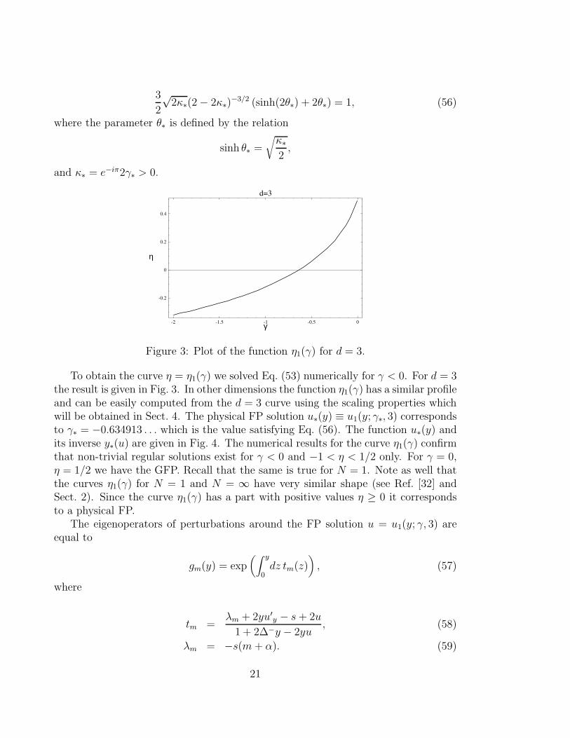
3

2

√2κ∗(2− 2κ∗)

−3/2 (sinh(2θ∗) + 2θ∗) = 1, (56)

where the parameter θ∗ is defined by the relation

sinh θ∗ =

√

κ∗

2,

and κ∗ = e−iπ2γ∗ > 0.

-2 -1.5 -1 -0.5 0

γ

-0.2

0

0.2

0.4

η

d=3

Figure 3: Plot of the function η1(γ) for d = 3.

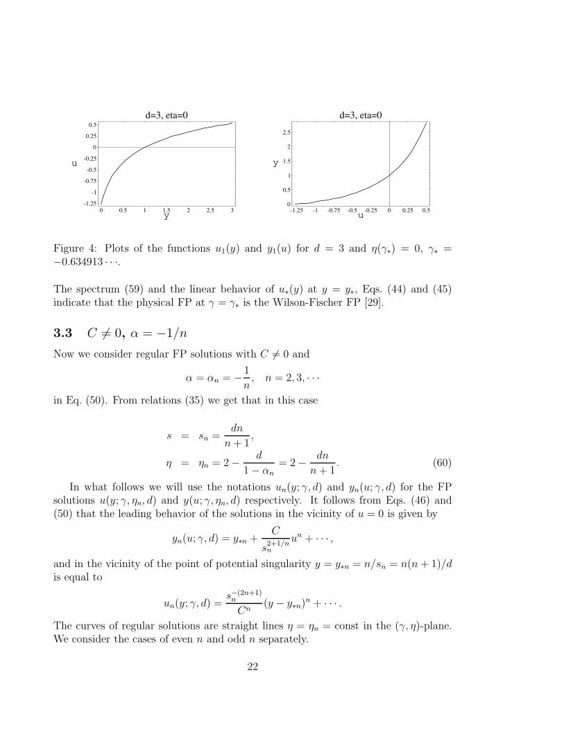
To obtain the curve η = η1(γ) we solved Eq. (53) numerically for γ < 0. For d = 3the result is given in Fig. 3. In other dimensions the function η1(γ) has a similar profileand can be easily computed from the d = 3 curve using the scaling properties whichwill be obtained in Sect. 4. The physical FP solution u∗(y) ≡ u1(y; γ∗, 3) correspondsto γ∗ = −0.634913 . . . which is the value satisfying Eq. (56). The function u∗(y) andits inverse y∗(u) are given in Fig. 4. The numerical results for the curve η1(γ) confirmthat non-trivial regular solutions exist for γ < 0 and −1 < η < 1/2 only. For γ = 0,η = 1/2 we have the GFP. Recall that the same is true for N = 1. Note as well thatthe curves η1(γ) for N = 1 and N = ∞ have very similar shape (see Ref. [32] andSect. 2). Since the curve η1(γ) has a part with positive values η ≥ 0 it correspondsto a physical FP.

The eigenoperators of perturbations around the FP solution u = u1(y; γ, 3) areequal to

gm(y) = exp(∫ y

0dz tm(z)

)

, (57)

where

tm =λm + 2yu′

y − s+ 2u

1 + 2∆−y − 2yu, (58)

λm = −s(m+ α). (59)

21

0 0.5 1 1.5 2 2.5 3y

-1.25

-1

-0.75

-0.5

-0.25

0

0.25

0.5

u

d=3, eta=0

-1.25 -1 -0.75 -0.5 -0.25 0 0.25 0.5u

0

0.5

1

1.5

2

2.5

y

d=3, eta=0

Figure 4: Plots of the functions u1(y) and y1(u) for d = 3 and η(γ∗) = 0, γ∗ =−0.634913 · · ·.

The spectrum (59) and the linear behavior of u∗(y) at y = y∗, Eqs. (44) and (45)indicate that the physical FP at γ = γ∗ is the Wilson-Fischer FP [29].

3.3 C 6= 0, α = −1/n

Now we consider regular FP solutions with C 6= 0 and

α = αn = −1

n, n = 2, 3, · · ·

in Eq. (50). From relations (35) we get that in this case

s = sn =dn

n+ 1,

η = ηn = 2− d

1− αn

= 2− dn

n+ 1. (60)

In what follows we will use the notations un(y; γ, d) and yn(u; γ, d) for the FPsolutions u(y; γ, ηn, d) and y(u; γ, ηn, d) respectively. It follows from Eqs. (46) and(50) that the leading behavior of the solutions in the vicinity of u = 0 is given by

yn(u; γ, d) = y∗n +C

s2+1/nn

un + · · · ,

and in the vicinity of the point of potential singularity y = y∗n = n/sn = n(n + 1)/dis equal to

un(y; γ, d) =s−(2n+1)n

Cn(y − y∗n)

n + · · · .

The curves of regular solutions are straight lines η = ηn = const in the (γ, η)-plane.We consider the cases of even n and odd n separately.

22

0 0.2 0.4 0.6 0.8 1

γ0

10

20

30

40

50

60

C

d=3, n=2

Figure 5: Plot of the function C2(γ) for d = 3.

3.3.1 n even

In this case a solution yn(u; γ, d) has two branches. As it was discussed earlier,the branch which satisfies 0 ≤ yn(u; γ, d) ≤ y∗n is given by formula (33) with theintegration constant equal to

Cn(γ) = −(2γ)αn(sn − 2γ)1−αn

αn+

αn − 1

αn

∫ 2γ

0

(

sn − z

z

)−αn

dz

(cf. (52)). This expression is a consequence of the initial condition, Eq. (32).For n even the function Cn(γ) and the solution yn(u; γ, d) exist for 0 < γ < sn/2.

In particular, for n = 2 one gets

C2(γ) = +3s2 arcsin

√

2γ

s2+ 2

√

s2 − 2γ

2γ(s2 + γ),

with s2 = 2d/3. The plot of the function C2(γ) for d = 3 is presented in Fig. 5.For each value of γ ≥ 0 and γ < sn/2 the two branches of the solution yn(u; γ, d)

are given by:for 0 ≤ u ≤ 2γ, 0 ≤ yn(u) ≤ y∗n

y(u) = − Cn(γ)

uα(s− u)2−α− 1

α(s− u)+

α− 1

α

1

uα(s− u)2−α

∫ u

0

(

s− z

z

)−α

dz (61)

= − u1/n

(s− u)2+1/nCn(γ)−

n

(sn − u)+

(n + 1)u1/n

(sn − u)2+1/n

∫ u

0

(

sn − z

z

)−α

dz;

for 0 ≤ u ≤ s, y∗n ≤ yn(u) < ∞

y(u) =Cn(γ)

uα(s− u)2−α− 1

α(s− u)+

α− 1

α

1

uα(s− u)2−α

∫ u

0

(

s− z

z

)−α

dz (62)

23

2 4 6 8 10y

0.25

0.5

0.75

1

1.25

1.5

1.75

2

u

d=3, n=2

0.25 0.5 0.75 1 1.25 1.5 1.75 2u

2

4

6

8

10

y

d=3, n=2

Figure 6: Plots of the functions u2(y) and y2(u) for d = 3 and γ = 1/2.

=u1/n

(s− u)2+1/nCn(γ)−

n

(sn − u)+

(n+ 1)u1/n

(sn − u)2+1/n

∫ u

0

(

sn − z

z

)−α

dz.

Formulas (61), (62) match together at u = 0. These two branches define a uniquefunction un(y; γ, d) for y ≥ 0. In Fig. 6 we show the plots of the functions u2(y; 1/2, 3)and y2(u; 1/2, 3) respectively.

It is easy to see that Cn(γ) → +∞ when γ → 0+. This limit, of course, corre-sponds to the GFP. For γ = sn/2 we find

Cn(sn/2) = ndπαn

sin(παn)=

πd

sin πn

.

The corresponding regular solution is un(y; sn/2, d) = sn = const, the TFP. Thisfunction is not invertible, hence the corresponding solution yn(u; sn/2, d) does notexist at γ = sn/2.

3.3.2 n odd

For n odd, n ≥ 3, regular solutions exist only for negative γ and consist of onebranch. The function yn(u; γ, d) is defined for 2γ ≤ u < s and varies in the range0 ≤ yn(u; γ, d) < ∞. The integration constant C in formula (33) is fixed by the initialcondition, Eq.(32), and is given by Eq. (52). As before, we denote it by Cn(γ). It iseasy to see that for odd n as κ = e−iπn2γ → 0+

Cn(γ) ∼ −nκ− 1

n s1−αn

n → −∞,

The plot of the function C3(γ) for d = 3 is shown in Fig. 7. The solutions u3(y;−1, 3)and y3(u;−1, 3) are given in Fig. 8.

Note the characteristic cubic root behavior of y3(u;−1, 3) in the vicinity of u = 0(see Eq. (50)).

24

-1.5 -1.25 -1 -0.75 -0.5 -0.25 0

γ

-70

-60

-50

-40

-30

-20

-10

0

C

d=3, n=3

Figure 7: Plot of the function C3(γ) for d = 3.

0.5 1 1.5 2 2.5 3 3.5 4y

-1.5

-1

-0.5

0

0.5

1

u

d=3, n=3

-1.5 -1 -0.5 0 0.5 1u

0.5

1

1.5

2

2.5

3

3.5

4

y

d=3, n=3

Figure 8: Plots of the functions u3(y) and y3(u) for d = 3 and γ = −1.

25

-4 -3 -2 -1 0 1u

0.5

1

1.5

2

2.5

3

3.5

4

y

d=3, n=3

Figure 9: Plot of the function y3(u) for d = 3 and γ = −2.5. The function isnon-monotonous in a vicinity of u = 0.

At certain value γ = γ∗n < 0 the function Cn(γ) = 0. Of course, this is thepoint where the straight line η = ηn (n = 3, 5, . . .) in the (γ, η)-plane hits the curveη = η1(γ) obtained in Sect. 3.1.

The solution un(y; γ∗n, d) coincides with u1(y; γ∗n, d) for this value of γ. Whentrying to search for solutions for γ < γ∗n one finds out that yn(u; γ, d) becomesnon-monotonous, and hence non-invertible, in a vicinity of u = 0, and therefore thesolution un(y; γ, d) does not exist. An example of such behavior is illustrated in Fig. 9which shows the plot of the function y3(u;−2.5, 3).

The eigenoperators are of the same form as in Eqs. (57) and (58). The eigenvaluesare given by

λnm = sn(1−

m

n). (63)

Note that these are also the eigenvalues of the GFP.

Let us summarize the results obtained in this section. We have found the infinitediscrete series of lines η = ηn(γ) (n = 1, 2, 3, . . .) located in a certain region of theparameter space (γ, η). Points on these lines correspond to regular FP solutions ofthe N = ∞ Polchinski ERG equation in leading approximation. The curve η1(γ) (seeFig. 3) bounds the region from the left. From the right the region is bounded by thestraight line η = 2 − 2γ of TFP solutions u = s. The curves η = ηn, n = 2, 3, . . .,are straight horizontal lines (see Eq. (60)). They start at γ = 0 (GFP solution) andend up either at γ = sn/2 > 0 (the TFP solution) for n even, or at γ = γ∗n < 0 forn odd. The value γ∗n is defined by the condition η1(γ∗n) = ηn. As n → ∞ the linesη = ηn accumulate at η∞ = 2− d.

26

4 Solutions for finite N and their N → ∞ limit

In the sections above we have seen a detailed treatment of the Polchinski ERG equa-tion for N = 1 and N = ∞. Not presented there are the finite N cases, that are ofinterest in their own right, but also because the N = ∞ case should be viewed as alimiting case for large N . For that reason, we present in this section a study of thefinite N case, and show how the N = ∞ case comes about as a limit.

First of all from the plots for N = 1 in Fig. 1 it is easy to notice that the patternsof the curves of regular solutions are the same for d = 2 and d = 3. They differ justby a vertical shift. Our analysis in the previous section shows that this is also truein the N = ∞ case. It turns out that for a given N the pattern of the curves ηn(γ)is universal and does not depend on the dimension of the space d. Namely, when wepass from one number of dimensions d to another d the functions ηn(γ) experiencea constant shift and some scaling transformation while the pattern of the curves ispreserved. This is a consequence of a property of the ERG equation which we aregoing to analyze in the remainder of this section.

Let u(y; γ, η, d) be a regular solution of (17), (18) corresponding to a point of acurve η = ηn(γ). Perform a scaling transformation

u(y) → u(y) = λu(y; η, γ, d), y =1

λy.

It is easy to check that the function u(y) satisfies the equation

2y

N

d2

dy2u(y)− 2yu

du

dy− u2 +

(

1 +2

N+ 2y∆−λ

)

du

dy+ sλu = 0, (64)

u(0) = 2γ ≡ 2λγ. (65)

Therefore u(y) is a regular solution in d dimensions corresponding to the point (γ, η)of the curve η = ηn(γ), where γ, η, d and a relation between ηn(γ) and ηn(γ) can befound from Eqs. (64) and (65) as follows. According to Eqs. (5) and (16), η = 2− s,d = s − 2∆−. Correspondingly, η = 2 − s, d = s− 2∆−, where ∆− = λ∆−, s = λs,see Eq. (64). Combining these relations we obtain that

d = λd, γ = λγ,

η = 2− λs = 2− λ(2− η) = 2(1− λ) + λη.

Trading λ for d/d we arrive at the relation

ηn(γ) = 2

(

1− d

d

)

+d

dηn

(

d

dγ

)

. (66)

This formula is valid for any N ≥ 1.

27

Eq. (66) can be rewritten as the relation

ηn(dγ)− 2

d=

ηn(dγ)− 2

d

which tells that the combination βn(γ) ≡ (ηn(dγ)− 2)/d is in fact independent of d.Therefore, a general solution of functional equation (66) is given by

ηn(γ) = 2 + dβn

(

γ

d

)

. (67)

The functions ηn(γ) studied in the previous sections do have this property. Wechecked that in the case N = 1 and d = 2 or d = 3, the curves ηn(γ) verify relation(66) or, equivalently, are described by (67). Special limits ∆+ = 0, ∆− = 0 areconsistent with (66), (67) as well. The results for the N → ∞ case in Sect. 3 are alsoin a full correspondence with this property. In particular, from Eqs. (54) and (60) itfollows that

βn

(

γ

d

)

= − 1

1− αn

(

γd

) .

Recall that for n ≥ 2 αn is the constant function αn = −1/n.For d fixed the shape of the curves changes with N . For N = 1, d = 2, 3, a few

curves are shown in Fig. 1. For N = ∞, d = 3 the plot of η1(γ) is given in Fig. 3.For n ≥ 2 ηn = 2− dn/(n+ 1) = const, i.e., they are represented by horizontal lines.It is of interest to study the curves for finite N > 1 and understand the transitionfrom N = 1 to N = ∞. In particular, a natural question arises: Do the intersectionsof the curves ηn(γ) (n odd, n ≥ 3) with the curve η1(γ), encountered for N = ∞,have an equivalent for finite N? Such intersections do not exist for N = 1. Is therea value of N for which intersections are encountered, or the N = ∞ curves approachthe large N limit in some other way?

To gain more insight into the properties of the functions ηn(γ) for an arbitraryN it is useful to study their behavior in the vicinity of γ = 0. This can be doneby a perturbative analysis for small values of γ. To this end, perform the change ofvariables v = −N∆−y, u(y) = 2γh(v). Eqs. (17) and (18) turn into

L(v)h− E h +2γ

∆−v h h′

z +γ

∆−h2 = 0, (68)

h(0) = 1, (69)

where

E =s

2∆−, L(v)h = v h

′′

vv + (M − z)h′v

and

28

M =N

2+ 1.

The linearized equation L(v)h = E h can be solved using the known solutions ofthe eigenvalue problem L(v)hn = λnhn:

λn = −n, hn(v) = Φ(−n,M ; v), n = 0, 1, 2, · · · , (70)

where

Φ(a, b; v) = 1 +a

bv +

(a)2(b)2

v2

2!+ · · · ,

(a)n = a(a+ 1) . . . (a+ n− 1), (a)0 = 1,

denotes the confluent hypergeometric function (see Ref. [45]). Note that hn(v) is apolynomial of order n with hn(0) = 1.

We now develop perturbation theory around these solutions. Fixing n, we write

h(v) = (1 + γD1 + γ2D2 + · · ·)(hn(v) + γ∑

k 6=n

ckhk + γ2∑

k 6=n

dkhk + · · ·),

E = E(0)n + γE(1)

n + γ2E(2)n + · · ·

(here Dn are constants) and solve system (68), (69) order by order in γ. Note that,at any order, the sums over k 6= n are over a finite number of terms. Here we list afew results.

At order γ0, we find En = E(0)n = −n, from which it follows that

ηn = 2− n d

n+ 1+O(γ), (71)

a result that is independent of N . A more detailed calculation yields

η0(γ) = 2− 2γ,

η1(γ) = 2− d

2+ 2γ(1 +

3

M) + γ224

d(1 +

13

M+

12

M2) +O(γ3),

η2(γ) = 2− 2d

3− 8γ

3M + 8

M(M + 1)+O(γ2),

η3(γ) = 2− 3d

4+ 6γ

3M2 + 69M + 196

M(M + 1)(M + 2)+O(γ2),

η4(γ) = 2− 4d

5− 48γ

15M2 + 215M + 636

M(M + 1)(M + 2)(M + 3)+O(γ2),

29

η5(γ) = 2− 5d

6+ 80γ

5M3 + 360M2 + 4225M + 12846

M(M + 1)(M + 2)(M + 3)(M + 4)+O(γ2),

η6(γ) = 2− 6d

7− 960γ

35M3 + 1365M2 + 14308M + 44364

M(M + 1)(M + 2)(M + 3)(M + 4)(M + 5)+O(γ2).

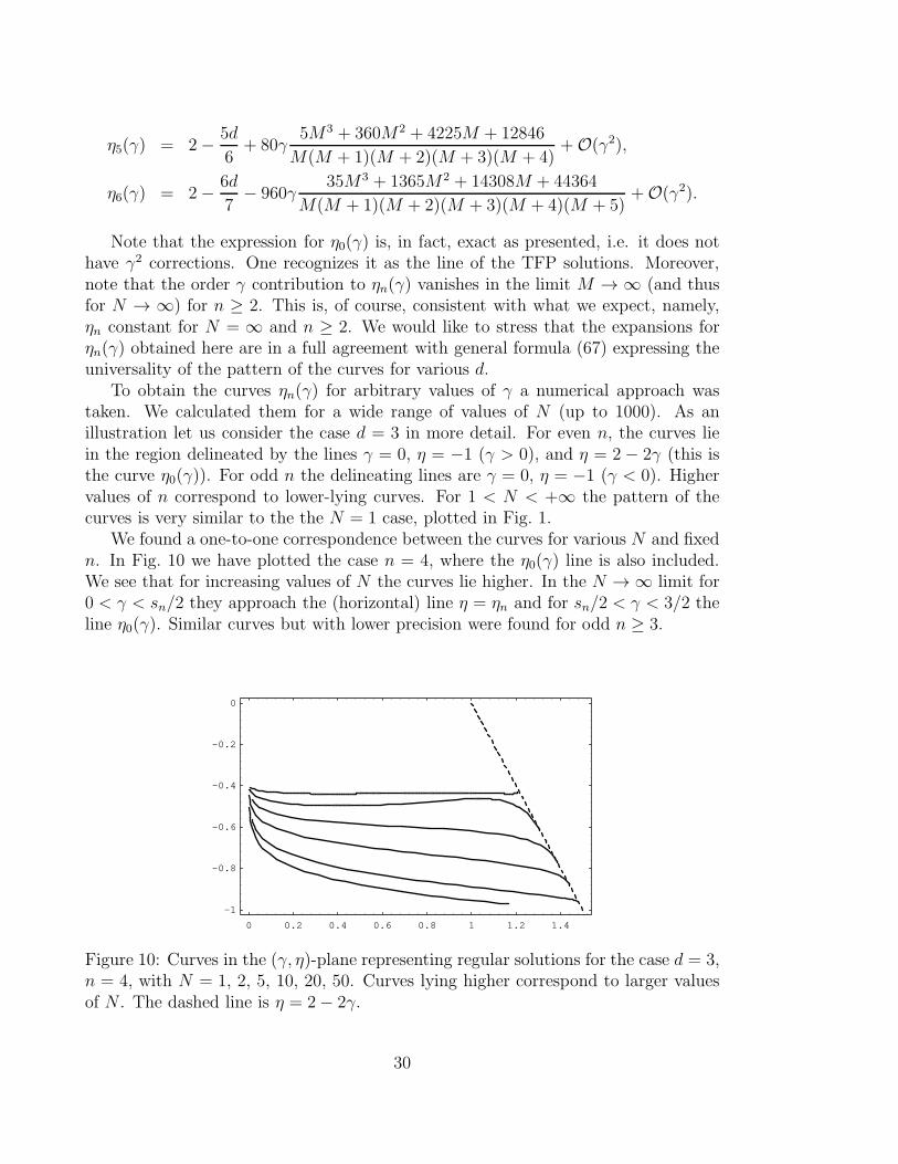
Note that the expression for η0(γ) is, in fact, exact as presented, i.e. it does nothave γ2 corrections. One recognizes it as the line of the TFP solutions. Moreover,note that the order γ contribution to ηn(γ) vanishes in the limit M → ∞ (and thusfor N → ∞) for n ≥ 2. This is, of course, consistent with what we expect, namely,ηn constant for N = ∞ and n ≥ 2. We would like to stress that the expansions forηn(γ) obtained here are in a full agreement with general formula (67) expressing theuniversality of the pattern of the curves for various d.

To obtain the curves ηn(γ) for arbitrary values of γ a numerical approach wastaken. We calculated them for a wide range of values of N (up to 1000). As anillustration let us consider the case d = 3 in more detail. For even n, the curves liein the region delineated by the lines γ = 0, η = −1 (γ > 0), and η = 2 − 2γ (this isthe curve η0(γ)). For odd n the delineating lines are γ = 0, η = −1 (γ < 0). Highervalues of n correspond to lower-lying curves. For 1 < N < +∞ the pattern of thecurves is very similar to the the N = 1 case, plotted in Fig. 1.

We found a one-to-one correspondence between the curves for various N and fixedn. In Fig. 10 we have plotted the case n = 4, where the η0(γ) line is also included.We see that for increasing values of N the curves lie higher. In the N → ∞ limit for0 < γ < sn/2 they approach the (horizontal) line η = ηn and for sn/2 < γ < 3/2 theline η0(γ). Similar curves but with lower precision were found for odd n ≥ 3.

0 0.2 0.4 0.6 0.8 1 1.2 1.4

-1

-0.8

-0.6

-0.4

-0.2

0

Figure 10: Curves in the (γ, η)-plane representing regular solutions for the case d = 3,n = 4, with N = 1, 2, 5, 10, 20, 50. Curves lying higher correspond to larger valuesof N . The dashed line is η = 2− 2γ.

30

Within the accuracy of the computation it can be concluded that as N grows thefunctions ηn(γ), existing for −∞ < γ < 0, transform to ηn =const, existing only forγ∗n < γ < 0. The latter is the limit we expect from our studies of the case N = ∞ inSect. 3.

5 Discussion and conclusions

We studied families of regular FP solutions of the Polchinski ERG equation for theO(N)-model in the LPA. The families are labeled by the integer n ≥ 1 and arerepresented by curves ηn(γ) in the (γ, η)-plane. We proved that for given N thepattern of the curves is universal for all d and described by Eq. (67).

There is a one-to-one correspondence between the curves for different N . Inparticular, for any N

ηn(0) = 2− nd

n+ 1,

see Eq.(71), and ηn → 2− d as γ → −∞ for n odd. Further properties of the curveswere discussed in detail in Sect. 4.

As N increases the η1(γ) curve transforms into the corresponding curve for N =∞. The rest of the curves transform into the straight lines given by Eq. (60).

For the N = ∞ case the solutions were studied analytically. We have shownthat most of them have a singularity at some finite point (see Eq. (41)) and are notacceptable from the physical point of view. The condition of regularity imposes arelation between the parameters η and γ. We analyzed this condition of regularityexplicitly and demonstrated how various classes of FP solutions appear.

The analysis of the N = ∞ case, carried out in the article, gives an explicitanalytical illustration of the condition which selects regular solutions. This enablesto get an insight into the nature of FP solutions of the ERG equations in the LPA.Usually these equations are stiff, and gaining a better understanding of the behaviorof its solutions is quite valuable.

We would like to mention that the pattern of the curves resembles the pattern ofeigenvalues (ηn) of an eigenvalue problem with a parameter (γ). As the parametervaries the levels change and various phenomena, like level crossing, may occur.

The results can be extended to higher order approximations of the Polchinski ERGequation. In particular, as it was mentioned in the Introduction, the regular solutionsstudied here can be used as initial input in the iteration procedure used for solvingthe next-to-leading order approximation. Methods of the analysis and the obtainedresults can also be useful in studies of ERG equations of other types in scalar models,as well as in other classes of theories, in particular in fermionic theories.

31

Acknowledgments

We would like to thank T.R. Morris for useful discussions and valuable comments.We acknowledge financial support from the Portuguese Fundacao para a Ciencia e aTecnologia (F.C.T.) under grants CERN/P/FIS/40108/2000, PRAXIS/2/2.1/FIS/-286/94, POCTI/FIS/32694/2000 and fellowships PRAXIS/BPD/14137/97, SFRH-/BPD/7182/2001.

References

[1] K.G. Wilson, Phys. Rev. B4, 3174, 3184 (1971); K.G. Wilson and J.B. Kogut,Phys. Rep. C12, 75 (1974).

[2] S. Ma, Rev. Mod. Phys. 45, 589 (1973).

[3] F.J. Wegner and A. Houghton, Phys. Rev. A8, 401 (1973).

[4] S. Weinberg, in Understanding the Fundamental Constituents of Matter, Erice1976, ed. A. Zichichi (Plenum Press, New York, 1978).

[5] J. Polchinski, Nucl. Phys. B231, 269 (1984).

[6] A. Hasenfratz and P. Hasenfratz, Nucl. Phys. B270, 687 (1986).

[7] T.R. Morris, in New Developments in Quantum Field Theory, NATO ASI Series366, (Plenum Press, New York, 1998), p. 147, hep-th/9709100; Prog. Theor.

Phys. Suppl. 131, 395 (1998) [hep-th/9802039]; in The Exact Renormalization

Group, ed. A. Krasnitz et al. (World Scientific, 1999), p. 1, hep-th/9810104.

[8] Yu.A. Kubyshin, Int. J. Mod. Phys. B12, 1321 (1998).

[9] C. Bagnuls and C. Bervillier, Phys. Rep. 348, 91 (2001).

[10] D.-U. Jungnickel and C. Wetterich, in The Exact Renormalization Group, ed.A. Krasnitz et al. (World Scientific, 1999), p. 41, hep-th/9710397; C. Wetterich,Int. J. Mod. Phys. A16, 1951 (2001); J. Berger, N. Tetradis and C. Wetterich,Phys. Rep. 363, 233 (2002).

[11] Yu.M. Ivanchenko and A.A. Lisyansky, Physics of Critical Phenomena (Springer,New York, 1995).

[12] R.D. Ball and R.S. Thorne, Annals. Phys. 236, 117 (1994).

[13] J.F. Nicoll and T.S. Chang, Phys. Lett. A62, 287 (1977).

[14] T.S. Chang, D.D. Vvedensky and J.F. Nicoll, Phys. Rep. 217, 279 (1992).

32

[15] M. Bonini, M. D’Attanasio, and G. Marchesini, Nucl. Phys. B409, 441 (1993).

[16] C. Wetterich, Phys. Lett. B301, 90 (1993).

[17] T.R. Morris, Int. J. Mod. Phys. A9, 2411 (1994).

[18] J.I. Latorre and T.R. Morris, J. High Energy Phys. 0011, 004 (2000); Int. J.Mod. Phys. A16, 2071 (2001); S. Arnone, A. Gatti and T.R. Morris, J. HighEnergy Phys. 0205, 059 (2002).

[19] A. Margaritis, G. Odor, and A. Patkos, Z. Phys. C39, 109 (1988); M. Alford,Phys. Lett. B336, 237 (1994).

[20] R.J. Myerson, Phys. Rev. B12, 2789 (1975).

[21] G.R. Golner, Phys. Rev. B33, 7863 (1986).

[22] T.R. Morris, Phys. Lett. B329, 241 (1994).

[23] T.R. Morris, Phys. Lett. B334, 355 (1994).

[24] P.E. Haagensen, Yu.A. Kubyshin, J.I. Latorre and E. Moreno, Phys. Lett. B323,330 (1994); in Proceedings of the International Seminar ”Quarks-94”, ed. D.Yu.Grigoriev et al. (World Scientific, 1995), p. 422, hep-th/9408050.

[25] J.F. Nicoll, T.S. Chang and H.E. Stanley, Phys. Rev. Lett. 33, 540 (1974); Phys.Rev. A13, 1251 (1976); V.I. Tokar, Phys. Lett. A104, 135 (1984).

[26] R.D. Ball, P.E. Haagensen, J.I. Latorre and E. Moreno, Phys. Lett. B347, 80(1995).

[27] T.R. Morris, Phys. Lett. B345, 139 (1995).

[28] T.R. Morris, Nucl. Phys. Proc. Suppl. 42, 811 (1995); Nucl. Phys. B458 [FS],477 (1996); Phys. Rev. Lett. 77, 1658 (1996); Int. J. Mod. Phys. B12, 1343(1998); Nucl. Phys. B495, 477 (1997).

[29] J. Comellas and A. Travesset, Nucl. Phys. B498, 539 (1997).

[30] T.R. Morris and M.D. Turner, Nucl. Phys. B509, 637 (1998); M. D’Attanasioand T.R. Morris, Phys. Lett. B409, 363 (1997).

[31] J. Comellas, Nucl. Phys. B509, 662 (1998).

[32] Yu.A. Kubyshin, R. Neves and R. Potting, in The Exact Renormalization Group,ed. A. Krasnitz et al. (World Scientific, 1999), p. 159, hep-th/981151.

[33] Yu.A. Kubyshin, R. Neves and R. Potting, Int. J. Mod. Phys. A16, 2065 (2001).

33

[34] T.R. Morris and J.F. Tighe, J. High Energy Phys. 9908, 007 (1999); Int. J.Mod. Phys. A16, 2095 (2001).

[35] G. Felder, Comm. Math. Phys. 111, 101 (1987).

[36] A.E. Filippov, Theor. Math. Phys. 91, 551 (1992); A.E. Filippov and S.A. Breus,Phys. Lett. A158, 300 (1991); Physica A192, 486 (1993).

[37] N. Tetradis and C. Wetterich, Nucl. Phys. B422, 541 (1994).

[38] J. Comellas, Yu.A. Kubyshin and E. Moreno, Nucl. Phys. B490, 653 (1997).

[39] T.R. Morris, Nucl. Phys. B573, 97 (2000) [hep-th/9910058]; J. High Energy

Phys. 0012, 012 (2000).

[40] S. Ma, Phys. Lett. A43, 479 (1973).

[41] F. David, D.A. Kessler and H. Neuberger, Phys. Rev. Lett. 53, 2071 (1984);Nucl. Phys. B257, 695 (1985).

[42] J. Zinn-Justin, Quantum Field Theory and Critical Phenomena (ClarendonPress, Oxford, 1993); Phys. Rep. 344, 159 (2001).

[43] G. Zumbach, Nucl. Phys. B413, 754 (1994).

[44] M. Reuter, N. Tetradis and C. Wetterich, Nucl. Phys. B401, 567 (1993).

[45] I.S. Gradshteyn and I.M. Ryzhik, Tables of Integrals, Series and Products: 6th

Edition (Academic Press, San Diego, 2000).

34