Solution of the groundwater transportmanagement problem by sequential relaxation

David P. Ahlfeld*, Antigoni Zafirakou 1 & R. Guy RieflerResearch Center for Groundwater Remediation Design, Department of Civil and Environmental Engineering, U-37,

University of Connecticut, Storrs, CT 06269, USA

(Received 3 March 1995; revised 26 December 1995; accepted 29 April 1997)

A heuristic algorithm is presented for problems which are formulated to find anoptimal groundwater remediation strategy with constraints on confined groundwaterflow and contaminant transport. The problem is simplified by decoupling the transportconstraints from the hydraulic constraints to produce a linear hydraulic controloptimization problem. The solution is obtained by an iterative process in which theconstraints on hydraulic gradient are updated, using information from transportsimulation, and the hydraulic control problem is solved repeatedly. In effect, thetransport simulation is used to calibrate the head difference constraint values of thehydraulic control problem. The algorithm is described in detail and its convergence isdemonstrated on several examples. The advantages and limitations of the algorithmare discussed.q 1998 Elsevier Science Limited. All rights reserved

Key words:groundwater, transport management, sequential relaxation, optimization.

1 INTRODUCTION

The remedial design problem consists of selecting the loca-tions of wells and associated rates of pumping so as tosatisfy hydraulic control and solute concentration criteriawhile minimizing overall system cost. Numerous manage-ment models have been proposed which couple numericaloptimization methods with groundwater flow and contami-nant transport simulation models (for example, Refs.1–3).One of the more computationally challenging types ofmanagement models are those where concentrations areconstrained as a function of pumping rates at remediationwells. The relationship between concentration and pumpingis non-linear and non-convex. Formulations withconstrained concentrations are generally computationallyintensive.4,5

In this paper, a heuristic algorithm is described anddemonstrated for solving formulations in which concentra-tions are constrained. The method is based on decouplingthe concentration constraints from the remaining, relativelyeasy, hydraulic control problem. The full problem is solved

using an iterative technique. At each iteration the hydraulicconstraints are adjusted. The adjustment is based on simula-tion of contaminant transport using the optimal pumpingrates from the previous hydraulic control problem solution.Iterations cease when optimal pump rates converge.

The motivation for the work presented here is to exploitthe relatively low computational costs associated with thehydraulic control problem while incorporating the impact ofthe hydraulic control solution on contaminant transport intothe decision process. The method will ultimately produce aremedial strategy which is feasible and optimal with respectto the hydraulic control problem and satisfies the constraintson concentration. The approach can be viewed as calibratingthe constraints of the hydraulic control problem by examin-ing the response of the transport solution.

Another algorithm which has involved combined use ofboth flow and transport modeling without direct solution ofthe contaminant remediation problem is that by Atwood andGorelick.6 These authors presented a scheme in which acentral extraction well, with specified location and rate,was used and a set of hydraulic control wells around theperimeter of the plume were selected to produce a capturezone. In their approach, the hydraulic control wells had to beoutside the plume perimeter. A transport model was used topredict the approximate location of the plume over time for

Advances in Water ResourcesVol. 21, pp. 591–604, 1998q 1998 Elsevier Science Ltd

Printed in Great Britain. All rights reserved0309-1708/98/$19.00 + 0.00PII: S 0 3 0 9 - 1 7 0 8 ( 9 7 ) 0 00 2 1 - 3

591

*Corresponding author.1 Present address: Department of Civil and EnvironmentalEngineering, Tufts University, Medford, MA 02155, USA.

purposes of defining candidate well locations. The hydrauliccontrol model was solved and the resulting impact on trans-port was simulated. Modifications were made to the candi-date well locations to insure that the hydraulic control wellsremained outside of the plume boundary.

Datta and Peralta7 proposed a regional groundwatermanagement model in which a convective transport modelwas used to modify the solution of a regional hydrauliccontrol model. In their case, the derivative of concentrationin a cell with respect to head in that same cell was calculatedanalytically from the finite difference approximation. Theimpact of head changes on concentration in adjacent cellswas not directly incorporated.

2 MODELING GROUNDWATER FLOW ANDCONTAMINANT TRANSPORT

The system under study is represented by the well knownthree-dimensional, coupled model for areal groundwaterflow and transport of a non-decaying, adsorbing, desorbingsolute in a confined aquifer, and consists of three partialdifferential equations with appropriate boundary conditions:

=·K·=hþ∑np

k¼ 1qkd(xk, yk, zk) ¼ 0 (1)

v¼ ¹ K·=h (2)

=·vD·=c¹ v·=c¹∑np

k¼ 1qk(c¹ c0k)d(xk, yk, zk) ¼ vR

]c]t

(3)

where

K ¼ hydraulic conductivity tensor (l/t),h ¼ hydraulic head (l),np ¼ number of pumps,qk ¼ pump rate for pump located at point (xk, yk, zk)(l 3/t),d(xk, yk, zk) ¼ dirac delta function evaluated at point(xk, yk, zk) (1/l3),v ¼ average Darcy velocity vector (l/t),v ¼ porosity of aquifer medium (dimensionless),c ¼ contaminant concentration (m/l3),c0k ¼ contaminant concentration in pumped fluid atpump pointk (m/l3),R ¼ retardation coefficient (dimensionless),D ¼ hydrodynamic dispersion tensor (m2/t).

3 OPTIMIZATION FORMULATION FORHYDRAULIC CONTROL

The method to be described here is applicable to problemsin which constraints are placed on both heads and concen-trations. Ahlfeld and Heidari3 provide a detailed derivation

of head constrained problems. For purposes of demon-strating the approach the following optimization formula-tion is considered

minimize∑j[J

bjqj (4)

such that

hi $ hpi, l i [ L (5)

hi # hpi,u i [ U (6)

hi1 ¹ hi2 $ di i [ D (7)

qj # qpj j [ J (8)

ci,T(q) # cpi i [ I (9)

where q represents the vector of all extraction rates atcandidate well locations,qj is the extraction rate at locationj, andJ is the set of candidate well locations made availableto the optimizer. At optimality, the model sets a givenpump rate to a positive value indicating withdrawl at thatwell or zero if no pumping is needed.

The objective function (eqn (4)) provides a measure ofcost whereb j is a cost coefficient on pumping at locationj.Constraint eqn (5) and (6) place bounds on the head at nodei, wherehi , l* and hi ,u* are specified lower and upper boundvalues, andhi is the head at locationi that results from thestresses described byq as simulated by eqn (1). The setsLandU indicate the node points at which, respectively, lowerand upper bounds are placed on the heads. Constraint eqn(7) is used to force a gradient in the hydraulic flow field,either horizontally or vertically. Here,di is a specifiedbound on the difference in heads at node pointsi1 and i2(hi 1 andhi 2). D is the set of indices which identify node pairsat which requirements on the differences in heads areimposed. Constraint eqn (8) limits extraction rates to thebound expressed byqj*.

Finally, constraint eqn (9) requires that the concentrationbe less than or equal to a prespecified value at the end of theplanning horizon at observation points within the system.Here,ci* is the specified maximum concentration bound atnodei, ci,T(q) is the concentration at nodei at the last timeperiod of the simulation as a function of pump rates, andI isthe set of nodes at which system concentration behavior willbe observed.

Because of the linear form of eqn (1), constraint eqn (5)–(8) are linear functions of pumping. Thus, if constraint eqn(9) is neglected the resulting problem is a linear program3

which can be solved with the widely used simplex method.8

The largest cost associated with solving the linear hydrauliccontrol problem is the calculation of the response matrix.The response matrix consists of derivatives of hydraulichead with respect to pumping. The response matrix isoften computed by perturbation which requires a flow simu-lation for each candidate well.3,9 The response matrix willnot change during execution of the sequential relaxation

592 D. P. Ahlfeldet al.

algorithm. At each iteration only the right hand side of thelinear program is changed. Repeated solution of the linearprogram involves relatively small computational cost. Thecomputational advantage described here depends on thelinear form of all the constraint equations except thoseinvolving concentration. Therefore, the aquifer thicknessmust be assumed independent of head; however, additionallinear constraints can be added to the formulation presentedhere.

4 HEURISTIC ALGORITHM FOR OPTIMALREMEDIAL DESIGN

The formulation described above is solved through a proce-dure involving decoupling and iteration. If the concentrationconstraint (eqn (9)) is relaxed the resulting problem is alinear program which is solved with modest computationaleffort. Given a particular solution to the hydraulic controlproblem, a simulation of the effect of the particular pumpingscheme on contaminant transport is performed. If the con-centration constraints do not satisfy certain criteria then theconstraints on head difference (which are synonymouslyreferred to as gradient constraints) are adjusted and thehydraulic control problem is resolved.

The functional relationships can be identified by definingL(d) as the linear programming operator which solves therelaxed problem given by eqns (4)–(8) mapping the headdifference constraint vector,d, to pumping rates (all con-straints other than eqn (7) are assumed fixed), andS(q) as thesimulation model operator which solves eqns (1)–(3) andmaps pumping rates to concentrations.

When viewed as a sequential process, it can be seen thatthe concentration vector,c, is a function of the head differ-ence constraints posed in the hydraulic control problem. Infunctional form this can be written as

q¼ L(d) (10)

c¼ S(q) (11)

or

c¼ S(L(d)) (12)

The key to the algorithm presented here is determination ofnew head difference constraints after evaluation of eqn(12). It is presumed that a robust relationship betweenhead difference constraints and concentration constraintsis present. This relationship can be assured by carefulplacement of candidate wells, head difference constraintsand concentration constraints in close proximity, so thateach concentration constraint can be unambiguously asso-ciated with a head difference constraint. The guidingrequirement for constraint placement is to insure thatmodification of head difference constraints will impactpumping rates at candidate wells which, in turn, willimpact concentrations at the associated concentration con-straint locations. If a head difference constraint does not

affect the optimal pumping (e.g. a head difference con-straint that is always satisfied), then concentration con-straints associated with that head difference constraintcannot be controlled.

The algorithm development proceeds by defining, foreach head difference locationi, a unique set of concentra-tion observation points,I i, such thatIi ∩ Ij ¼ 0 for all i notequal to j and I1 ∪ I2 ∪ … Ii ∪ … In ¼ I where n is thenumber of head difference constraint pairs inD. A firstorder Taylor Series expansion ofc, as described in eqn(12), about the head difference constraint value is per-formed. The vectorc can be approximated in terms of itsindividual elements by

ckþ 1l ¼ ck

l þ]cl

]di(dkþ 1

i ¹ dki ) l [ Ii , i ¼ 1, …, n (13)

where the superscripts indicate the iteration level. Note thatit is implicitly assumed in eqn (13) that the concentrationdepends only on theith head difference constraint. Thecriteria for selection ofdi

kþ1 is that the concentration thatresults from imposition of the new head difference con-straint value will satisfy constraint (9). This criteria isapproximated by imposing the requirement on eqn (13)that di

kþ1 be selected so that

ckþ 1l # cp

l (14)

Substituting eqn (13) into eqn (14) and rearranging yields

ckl þ

]cl

]di(dkþ 1

i ¹ dki ) # cp

l (15)

or

dkþ 1i # dk

i þ(cp

l ¹ ckl )

]cl =]di(16)

If the partial derivative in eqn (16) is approximated by

]cl

]di¼

(ckl ¹ ck¹ 1

l )(dk

i ¹ dk¹ 1i )

(17)

then eqn (16) can be used to provide a proposed change inhead difference constraint based on each of the associatedconcentration constraints. Hence, for theith head differenceconstraints the proposed changes are given by

dkþ 1i, l # dk

i þ(cp

l ¹ ckl )

(ckl ¹ ck¹ 1

l )(dk

i ¹ dk¹ 1i ) l [ Ii (18)

eqn (18) yields multiple proposed head difference con-straint values,di,l

kþ1, if the head difference constraint hasmultiple concentration constraints with which it is asso-ciated. In this circumstance, a prioritization method mustbe devised. Considering the inequality described in eqn(18), four cases can arise. They can be examined by con-sidering two factors: the sign of(cp

l ¹ ckl ) and the sign of

the gradient in eqn (17). To facilitate this considerationdefine

D¼(cp

l ¹ ckl )

(ckl ¹ ck¹ 1

l )(dk

i ¹ dk¹ 1i ) (19)

Groundwater transport management 593

Proposed head difference constraint changes which derivefrom locations where the concentration constraint are notsatisfied, i.e.cl . cl*, are given priority over all otherproposed constraint changes regardless of the sign of eqn(17). To satisfy all concentration constraints at the nextiteration, the maximum head difference change proposedis selected. Thus, theith head difference constraint ischosen to satisfy

dkþ 1i ¼ dk

i þ maxl[I p

i

lDlsign(D) (20)

where the setI i* is defined so thatl [ I pi if and only if l [ Ii

andcl . cpl . Note that the fact that eqn (19) may take on a

positive or negative sign is incorporated.If all the concentration constraints associated with theith

head difference constraint are satisfied as inequalities, thenthe head difference constraint can be relaxed until at leastone of the concentration constraints is binding. The direc-tion of change of the head difference constraint needed toachieve a binding concentration constraint will depend onthe sign of eqn (17). The magnitude of the change is deter-mined by the minimum proposed head difference change,since the observation point which generates the minimumproposed head difference is estimated to be the first to reachits bound. Thus, whencl # cl* for all l [ Ii , the ith con-straint head difference is chosen to satisfy

dkþ 1i ¼ dk

i þ minl[Ii

lDlsign(D) (21)

The algorithm can be stated concisely using the followingdefinitions;

qk ¼ vector of pump rates at iterationk,ck ¼ vector of concentrations at locations from setI atiterationk,dk ¼ vector of head difference requirements at loca-tions from setD at iterationk,d0 ¼ an initial guess of the head difference require-ments, andG(c) ¼ the head difference updating operator, summar-ized in eqns (19)–(21), which maps concentration toupdated head difference constraint values.

The algorithm proceeds as follows;

Step 1: Initializationsetq0 ¼ `setd0 ¼ d0

setc0 ¼ S(L(d0))setd1 ¼ d0 þ dd

setk ¼ 1Step 2: Solution of hydraulic control model

setqk ¼ L(dk)Step 3: Test for convergence

if kqk ¹ qk¹1` , d stopelse continue

Step 4: Solution of transport modelsetck ¼ S(qk)

Step 5: Update head difference requirementssetdkþ1 ¼ G(ck)

Step 6: Iteratesetk ¼ k þ 1 ; go to Step 2

Here dd is a perturbation of the initial head differenceconstraint value,k…k is a suitable norm of the indicatedquantity, andd is a specified convergence criteria. Eqns(19)–(21) define, in scalar form, the vector relation requiredin Step 5 of the algorithm.

It should be noted that the test for convergence is imposedon the pumping rates. Since pumping rates are the primarydecision variables of the formulation, their use in testing forconvergence is a natural choice. Examination of eqns (19)–(21) reveals that head difference constraints are not modi-fied, if all the concentration constraints are satisfied, and atleast one concentration constraint associated with each headdifference constraint is binding. If the head difference con-straints are not modified, then the new pumping rates thatare derived from Step 2 will be unchanged from the previousiteration. Hence, convergence of the optimal pumping ratesimplies convergence of the head difference constraints, andin turn, convergence of the concentration constraints. Casesmay arise where all concentration constraints associatedwith a head difference constraint are satisfied as inequal-ities. Evaluation of eqn (21) would then dictate a change inthe head difference constraint value. However, if themodified head difference constraint is already satisfied,then the optimal pumping rates may not change at thenext iteration and the algorithm will terminate. As long asconcentration constraints are satisfied, such termination isacceptable.

One complication that may arise in execution of thisalgorithm is that a linear program created by updating ofthe head difference constraints in Step 5 may proveinfeasible when Step 2 is evaluated in the next iteration. Adirect method for accommodating this problem is to allowthe updating algorithm to select head differences accordingto the rules discussed above and attempt to solve the controlproblem. If the resulting control problem is infeasible, thenall gradient changes can be reduced by a factor. To quantifythis, define an updating factor alpha, with 0# a # 1, so thatthe updated gradients are calculated as

d̂k þ 1

¼ dk þ a(dk þ 1 ¹ dk) (22)

where d̂k þ 1

is the new head difference constraint used instep 2 of the algorithm. If the problem in step 2 isinfeasible, we seek to maximize alpha such that the con-straints are feasible.

5 DEMONSTRATION OF THE ALGORITHM

The algorithm described above has been implemented in asingle code which couples and repeatedly executes therespective flow and transport equations. In the tests to beconducted here these equations are solved using the codes

594 D. P. Ahlfeldet al.

MODFLOW10 for three-dimensional groundwater flow andMT3D11 for three-dimensional solute transport. Both ofthese codes employ the finite difference method. Testingof the algorithm that is presented here has been performedon a hypothetical problem solved on the 50003 2300 footfinite difference grid shown in Fig. 1. A uniform gridspacing of 100 feet is used over the entire domain. Twomodel layers are represented, each with a thickness of 100feet, although, the model parameters in each layer are iden-tical and, for the results presented here, all constraints andpumping wells are located in the upper layer. The hydraulicconductivity is a uniform 10 feet/day, the porosity is 0.25,the non-pumping regional gradient is 0.02 and the disper-sivities are 45 and 17.5 feet, respectively, in the longitudinaland transverse directions. A plume is generated on this gridfrom a Dirichlet source with simulation conducted over a 10year period. The resulting plume, which will serve as initialconditions for subsequent optimization runs, is shown inFig. 2.

In a first example, designed to demonstrate the behaviorof the algorithm, a single pumping well is placed in thedomain along with a head difference constraint and concen-tration observation point. The arrangement of these problem

elements are shown in Fig. 3(a), where the open circle repre-sents the candidate well location, the heavy line representsthe location of the head difference constraint, the asteriskrepresents the location of the concentration observationpoint and the dashed line indicates the head difference con-straint to which the concentration constraint is associated.The candidate well, head difference constraint and observa-tion point are all numbered for convenience.

The concentration constraint imposed at the observationpoint is 5 concentration units after 10 years of remedialpumping. The algorithm converges after nine iterationsfrom an initial head difference constraint of 0.01 and initialconcentration at the concentration observation point of 26.The convergence behavior of the gradients required in eachhydraulic control problem, the pumping rates, and theresulting concentrations are shown in Table 1. The firstiteration uses the specified initial guess of the gradientvalue of 0.01. The second iteration uses a user-definedperturbed value of the initial gradient to produce the firstderivative of the form of eqn (17). Once begun, all thevariables in the algorithm follow a rapid, monotonicconvergence to the solution where the constraint is satisfiedto five digits of accuracy. The steady hydraulic head

Fig. 1. Cell-centered finite different grid for test problem.

Fig. 2. Initial concentration distribution for test problem.

Groundwater transport management 595

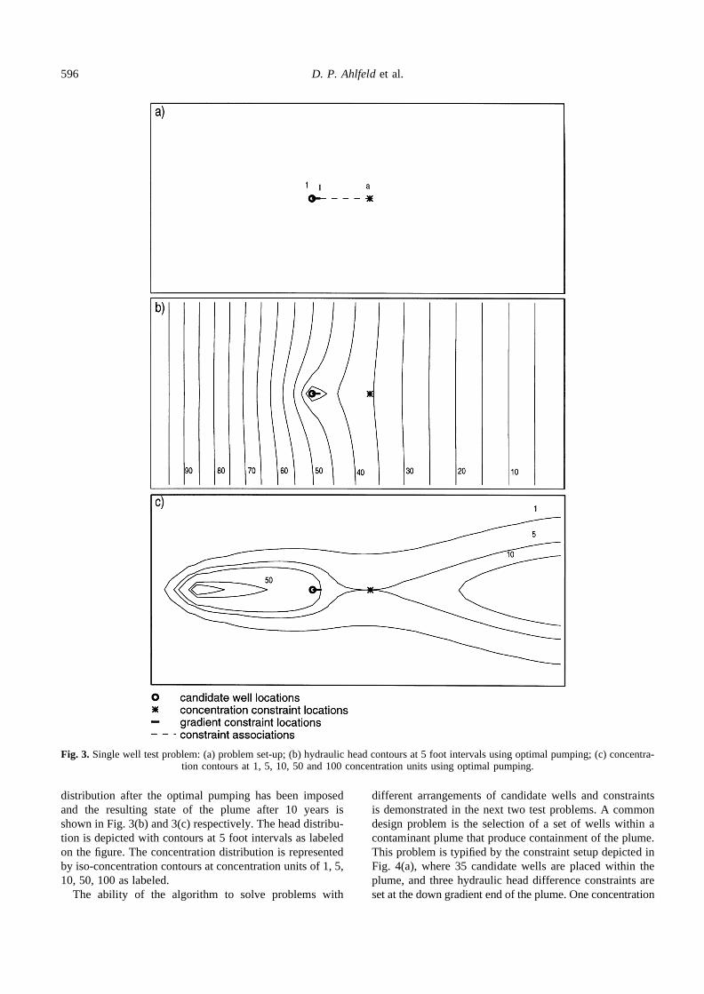
distribution after the optimal pumping has been imposedand the resulting state of the plume after 10 years isshown in Fig. 3(b) and 3(c) respectively. The head distribu-tion is depicted with contours at 5 foot intervals as labeledon the figure. The concentration distribution is representedby iso-concentration contours at concentration units of 1, 5,10, 50, 100 as labeled.

The ability of the algorithm to solve problems with

different arrangements of candidate wells and constraintsis demonstrated in the next two test problems. A commondesign problem is the selection of a set of wells within acontaminant plume that produce containment of the plume.This problem is typified by the constraint setup depicted inFig. 4(a), where 35 candidate wells are placed within theplume, and three hydraulic head difference constraints areset at the down gradient end of the plume. One concentration

Fig. 3. Single well test problem: (a) problem set-up; (b) hydraulic head contours at 5 foot intervals using optimal pumping; (c) concentra-tion contours at 1, 5, 10, 50 and 100 concentration units using optimal pumping.

596 D. P. Ahlfeldet al.

observation point is associated with each hydraulic headdifference constraint as shown. The resulting problem issolved successfully in 13 iterations. As can be seen in Fig.4(b) and 4(c), well 35 is selected and produces a schemewhich meets the specified standard at the observation points.This problem is symmetric about the longitudinal axis of theplume. An alternate solution would consist of pumping atwell 12 which would produce a plume that is symmetric to

that shown here. The choice of pumping wells can be seenby examining the iterative development of the solution forthis problem depicted in Table 2. The algorithm beginswith symmetric head difference constraints and a nearlysymmetric solution with pumping at both wells 12 and 35.However, because of round-off errors in computation of thehydraulic head solution the pumping is slightly different atthe two wells and the concentration at the symmetric points

Fig. 4. Multiple well containment problem: (a) problem set-up; (b) hydraulic head contours at 5 foot intervals using optimal pumping; (c)concentration contours at 1, 5, 10, 50 and 100 concentration units using optimal pumping.

Groundwater transport management 597

a and c are slightly different. This difference tips the solu-tion towards use of well 35. Note that at iteration 5 thegradients are set to zero in an attempt by the algorithm toincrease the concentrations at the observation points to theirstandard. This over-compensation produces violations atobservation point b which is corrected in subsequentiterations. It should also be noted that in these test problems,

a minimum head difference constraint value of 0.0 isestablished. In addition, a rule is imposed that introducesa specified increase in head difference constraint, when anyof the constraints associated with a head difference con-straint at 0.0 are violated. This rule is implemented initeration 9 of this test problem.

Another example is depicted in Fig. 5. Here, the scheme

Fig. 5. Longitudinal well containment problem: (a) problem set-up; (b) hydraulic head contours at 5 foot intervals using optimal pumping;(c) concentration contours at 1, 5, 10, 50 and 100 concentration units using optimal pumping.

598 D. P. Ahlfeldet al.

consists of pumping along the longitudinal axis of the plumeto prevent transverse spreading of contaminant. The headdifference constraints are associated with clusters of con-centration constraints located on the sides of the plume. Theassociations are indicated by the dashed lines connectinghead difference constraints with clusters of concentration

constraint locations on Fig. 5(a). The wells are placedaway from the centerline of the plume to produce anon-symmetric solution. This problem is readily solved in14 iterations with pumping rates of 12 746, 11 524 and27 004 cubic feet per day respectively at wells 1, 2 and 3.The hydraulic head and concentration surfaces produced by

Fig. 6. Head difference constraint interference problem: (a) problem set-up; (b) hydraulic head contours at 5 foot intervals using optimalpumping; (c) concentration contours at 1, 5, 10, 50 and 100 concentration units using optimal pumping.

Groundwater transport management 599

the optimal pumping solution are depicted in Fig. 5(b) and5(c), respectively. Concentration constraints at observationpoints f and r are binding at the solution. The headdifference constraints that control the pumping at wells 1and 3 are in turn controlled by the nearby binding concentra-tion constraints. The pumping at well 2 is due in large part tothe specified minimum head difference constraint of 0.0.

6 DISCUSSION OF POTENTIAL LIMITATIONS OFTHE ALGORITHM

Several limitations to the algorithm are possible. Theserelate to limitations of the general nature of the relationshipbetween gradients and concentrations and poor problem set-up. Several examples are provided to demonstrate these

Fig. 7. Multiple concentration constraint interference problem: (a) problem set-up; (b) concentration contours at 1, 5, 10, 50 and 100concentration units at iteration 22; (c) concentration contours at 1, 5, 10, 50 and 100 concentration units at iteration 23.

600 D. P. Ahlfeldet al.

limitations, and guidance is offered for appropriate use ofthe algorithm.

The primary postulate of this algorithm is that the rela-tionship between concentration and head difference con-straints is unique and reliable. This assumption forms thebasis for the updating method described in eqn (18). The useof this assumption has two subsidiary assumptions. First, itis assumed that changing a head difference constraint doesnot significantly affect those concentration values that arenot associated with that head difference constraint. That is,only a single gradient affects each concentration. Second,all concentrations that are affected by a given head differ-ence constraint are affected in a consistent manner—forexample, the concentrations increase or decrease together.The validity and significance of these two assumptions arediscussed in the examples below.

6.1 Influence of multiple head difference constraints ona single concentration

Intuitively, the assumption that a single concentration isonly affected by a single head difference constraint mightbe violated in circumstances where concentration at a singlelocation is affected by pumping at several wells. Hence, onemight expect that significant competition effects mightcause failure of the algorithm. While no proof can be offeredthat this will never be a problem, our experience indicatesthat this will not be the problem that might be imagined.

For example, consider the problem depicted in Fig. 6. Theproblem set-up is such that the concentrations at locations g,h, i, j, k, and l should be significantly impacted by pumpingat wells 2 and 3. However, these concentrations are linked togradients I and II which are closely associated with well 1.Despite this apparent potential for interaction, a solution isachieved after 53 iterations as depicted in Fig. 6(b) and 6(c).That interference is occurring can be seen from examinationof Table 3 which shows the gradients and pumping ratesassociated with wells 1 and 3 along with the concentrationsat location h over the first five iterations. At iteration 3,gradient I is driven to a value of 0.8109. This increase ingradient produces an increase in pumping at well 1 and adecrease in concentration at h. Having overshot the desireddecrease (the concentration is now below the standard), thealgorithm reduces gradient I at iteration 4 to get an increasein concentration at h to just meet the standard. However, atthe same iteration gradient III has increased causing well 3to increase its pumping. This causes a further reduction inpumping due to the interference between pumping at well 3and concentration at h. After one additional iteration, 5, thegradient increases again at I seeking to increase the concen-tration. The new hydro-chemical regime produced by largepumping at 3 responds and the concentration increases.Because the algorithm only utilizes information from thepast step, it is able to recover from a change in the type ofresponse that is encountered at the concentration responsepoint.

6.2 Multiple concentrations influencing a single headdifference constraint

Another possible problem is the association of several dis-tant concentration constraints with a single head differenceconstraint. The presumption made in the association of aconcentration constraint with a head difference constraintis that there exists a significant physical connection betweenthe two and that all concentration constraints connected tothe same head difference constraint have a similar responseto changes in that constraint. The appropriate level ofsignificance is a matter of judgment, however, multiple

Table 1. Convergence behavior for single well test problem

Iteration Gradient I Well 1 Concentration a

1 0.0100 ¹11 311.7 25.95182 0.0095 ¹11 308.9 25.95453 3.9585 ¹33 157.6 11.07134 5.5694 ¹42 070.2 7.86655 7.0103 ¹50 042.0 5.85806 7.6259 ¹53 447.8 5.18597 7.7961 ¹54 389.5 5.01878 7.8151 ¹54 494.6 5.00049 7.8155 ¹54 496.7 5.0000

Table 2. Convergence behavior for multiple well containment problem

Iteration Gradient I Gradient II Gradient III Well 12 Well 35 Concentration a Concentration b Concentration c

1 0.0100 0.0100 0.0100 ¹66 098.0 4.4073 4.4073 20.9961 4.440532 0.0095 0.0095 0.0095 ¹66 080.4 ¹66 081.8 4.4055 20.9982 4.40363 0.1757 3.7775 0.1769 0.0 ¹347 575.8 0.0054 0.0034 0.00184 0.0000 2.8808 0.0000 0.0 ¹293 935.9 0.0769 0.0626 0.03845 0.0000 0.0000 0.0000 ¹65 773.1 ¹65 774.6 4.3686 21.0336 4.36676 0.000 2.2025 0.0000 0.0 ¹23 367.6 0.5292 0.5714 0.41567 0.000 1.7258 0.000 0.0 ¹224 854.8 1.16181 2.3357 1.97508 0.000 1.0060 0.000 0.0 ¹181 798.3 2.6305 8.6080 11.38109 0.0000 1.4201 0.1000 0.0 ¹206 565.6 2.5626 4.8891 4.751210 0.000 1.4077 0.0962 0.0 ¹205 827.1 2.5932 5.0148 4.906711 0.000 1.4092 0.0940 0.0 ¹205 914.2 2.5896 4.9999 4.888212 0.0000 1.4092 0.1076 0.0 ¹205 913.9 2.5897 5.0000 4.888313 0.0000 1.4092 1.1076 0.0 ¹205 913.9 2.5897 5.0000 4.8883

Groundwater transport management 601

concentration constraints that are driven by substantiallydifferent physical phenomena linked to the same headdifference constraint can produce problems in performanceof the algorithm. An example of this behavior is provided inthe test problem depicted in Fig. 7. Here, concentrationconstraints are linked as shown in Fig. 7(a). After 19 itera-tions, the algorithm begins to oscillate in the solutionselected at each iteration. This behavior is depicted inTable 4 for iterations 20–40. In even numbered iterationsgradient I is lowered to satisfy constraint i. The pumpingrate at well 1 is dropped and constraint i is nearly satisfied.However, the decrease in pumping rates causes an increasein concentration at constraint c, where the constraint isviolated. In odd numbered iterations, gradient I is increasedto satisfy constraint c. The pumping rate is increased, andthe violation of constraints is reversed. The other headdifference constraints and pumping rates do not changeappreciably during these iterations. The apparentlycounter-intuitive response to pumping at constraints c andi is a result of the fact that they are in two different hydro-chemical regimes of the plume. On the upgradient side,increasing pumping at well 1 causes contraction of theplume and a reduction of concentrations at c. On the down-gradient side, increased pumping causes movement of ahigh concentration zone closer to constraint i. The plume

that is produced during even numbered iterations is shownin Fig. 7(b). The plume produced in odd numbered iterationsis shown in Fig. 7(c). It is clear that we are seeking a singlehead difference constraint (and associated pumping rate) tosatisfy conditions in two distinctly different portions of theplume. Because of this difference in response to pumping atthe two concentration constraints, no single gradient value(or associated pumping rate) can satisfy both constraints,and the algorithm fails. Hence, care must be taken toavoid assigning concentration constraints to head differenceconstraints that are not expected to respond in a similarfashion.

6.3 Non-monotonic convergence

In conventional gradient based algorithms, the objectivefunction (if minimized) is expected to decrease mono-tonically at each iteration. In fact, the proof of this descentis a necessary (but not sufficient) condition for proof ofconvergence.8 However, the present algorithm contains noguarantee that such descent will occur. Instead, the algo-rithm can be viewed as one in which the head differenceconstraints are adjusted to best coincide with the concentra-tion constraints. The initial constraint space is bounded bylinear hydraulic head difference constraints and non-linear

Table 3. Initial iterations for head difference constraint interference problem

Iteration Gradient I Gradient III Well 1 Well 3 Concentration h

1 0.0100 0.0100 ¹10 429.8 ¹10 301.9 6.01512 0.0095 0.0095 ¹10.429.8 ¹10 299.4 6.01583 0.8109 0.0095 ¹14 249.1 ¹9915.1 4.28644 0.4802 1.0095 ¹16 379.3 ¹14 282.7 1.35455 0.8914 2.3288 ¹15 358.5 ¹22 604.3 5.6478

Table 4. Iterations for the multiple concentration constraint interference problem showing oscillation of head difference constraintvalues.

Iteration Gradient I Gradient III Gradient IV Well 1 Well 2 Well 3 Concentration c Concentration i

20 39.3390 0.6063 5.5601 ¹188 433.3 ¹5146.3 ¹402.5 6.2879 3.569021 62.5194 0.6793 0.5590 ¹293 581.3 ¹212.6 ¹149.8 5.0017 14.862622 42.2761 0.6678 0.5590 ¹201 764.0 ¹4803.6 ¹4102.5 6.873 4.213523 62.5515 0.6777 0.5590 ¹293 726.8 ¹196.2 ¹144.2 5.0004 14.865924 43.7731 0.6762 0.5590 ¹208 554.9 ¹4504.8 ¹3807.4 5.9922 5.374825 62.5592 0.6774 0.5590 ¹293 761.5 ¹193.3 ¹142.7 5.0001 14.866426 43.0313 0.6773 0.5590 ¹205 190.6 ¹4681.1 ¹3.951.7 6.0384 4.716927 62.5604 0.6774 0.5590 ¹293 767.2 ¹192.8 ¹142.5 5.0000 14. 866428 43.5760 0.6774 0.5590 ¹207 661.1 ¹4556.6 ¹3845.4 6.0043 5.176029 62.5605 0.6774 0.5590 ¹293 767.8 ¹192.8 ¹142.5 5.0000 14.866330 43.2311 0.6774 0.5590 ¹206 096.9 ¹4636.0 ¹3912.6 6.0259 4.867531 62.5605 0.6774 0.5590 ¹293 767.8 ¹192.8 ¹142.5 5.0000 14.866432 43.4873 0.6774 0.5590 ¹207 258.9 ¹4577.1 ¹3862.7 6.0098 5.089533 62.5606 0.6774 0.5590 ¹293 768.2 ¹192.8 ¹142.5 5.0000 14.866434 43.3127 0.6774 0.5590 ¹206 467.2 ¹4.6172 ¹3896.7 6.1207 4.930235 62.5606 o.6774 0.5590 ¹293 768.1 ¹192.8 ¹142.5 5.0000 14.866436 43.4480 0.6774 0.5590 ¹207 080.5 ¹4586.1 ¹3870.3 6.0123 5.051837 62.5607 0.6774 0.5590 ¹293 768.5 192.7 ¹142.5 5.0000 14.866438 43.3470 0.6774 0.5590 ¹206 622.6 ¹4609.3 ¹3890.3 6.0186 4.959639 62.5606 0.6774 0.5590 ¹293 768.2 ¹192.8 ¹142.5 5.0000 14.866440 43.4254 0.6774 0.5590 ¹206 978.4 ¹4591.3 ¹3.874.7 6.0137 5.0306

602 D. P. Ahlfeldet al.

concentration constraints. During the course of the algo-rithm the concentration constraints are relaxed and the sim-plified problem is solved. The resulting solution is tested tosee if any of the relaxed concentration constraints areviolated or not binding. The head difference constraintsare then translated within the constraint space by adjustmentof the head difference constraint values to better coincidewith the concentration constraints in the vicinity of the solu-tion. Our extensive testing has indicated that situations mayarise in which small changes in head difference constraintvalues produce large rearrangements of pumping and sig-nificant changes in concentration. In these cases the objec-tive function may not decrease, and the solution may movefurther from satisfaction of the concentration constraints.However, the algorithm generally recovers from these cir-cumstances and eventually converges to a solution.

6.4 Computational performance

The primary advantage of the approach taken in this algo-rithm is computational efficiency. Repeated solution of thelinear program involves relatively small computational cost,since only the right hand side of the linear program ismodified. The only significant computational costs areinitial calculation of the response matrix and repeatedevaluation of the transport equation which is performedonce in each iteration of the algorithm. Other approachesto solving eqns (4)–(9) have included direct solution bygradient based non-linear optimization methods, the use ofdynamic programming, genetic algorithms, simulatedannealing and neural networks. In each of these cases thecomputational time is dominated by the need to repeatedlysolve eqn (3). While the limited testing performed to date onthe present algorithm is insufficient to confirm computa-tional superiority, some general observations can be made.The examples presented here that successfully convergedrequired less than 53 iterations with one evaluation of eqn(3) per iteration. Ahlfeld et al.4 report on an application thatis solved using gradient based optimization combined withadjoint sensitivity analysis that requires over 400 evalua-tions of eqn (3). Rogers and Dowla12 report an applicationsolved using neural networks that requires over 200 evalua-tions of eqn (3). Marryott et al.13 report an applicationsolved with simulated annealing that required over 2000evaluations of eqn (3), although they report that subsequentimprovements to the algorithm can reduce this substantially.Culver and Shoemaker5 utilize dynamic programming forsolution of multiple time period problems. While providingflexibility in formulation, these algorithms are generallyvery computationally intensive, requiring many times thecomputational effort required for the present algorithm.Comparison of these reported computational results mustbe treated with caution due to differences in computationalcosts for other portions of the algorithms and differences inthe applications reported; however, it is apparent that thepresent algorithm has the potential to solve problems of thistype with reasonable computational effort.

7 CONCLUSION

A new heuristic algorithm has been proposed for solvingproblems which are formulated to find an optimal ground-water remediation strategy with constraints on confinedgroundwater flow and contaminant transport. The algorithmis based on solving the hydraulic control problem repeatedlywhile modifying the head difference constraints. Theseconstraints are modified in response to the impact of optimalpumping on simulated concentration. The algorithmrequires that each concentration constraint be associatedwith a single head difference constraint, so that a relation-ship can be developed between the head difference con-straint and the concentration constraint.

The algorithm has been demonstrated to successfullyconverge on several test problems. These problems encom-pass several classes of possible arrangements of locations ofcandidate wells, head difference constraints and concentra-tion constraints for which the algorithm is intended. Thealgorithm can fail when multiple concentration constraintsthat are associated with a single head difference constraintexperience significantly different responses to changes inpumping. Interference by multiple wells in the relationshipbetween concentration and gradient constraints can alsocause failure of the algorithm in some circumstances. How-ever, the use of only prior iterate information assists thealgorithm in recovering from such interference events.The computational performance of this algorithm showspromise; however, problems described above with problemset-up, interference and convergence should cause cautionto be exercised in the implementation of this approach.

ACKNOWLEDGEMENTS

This work was funded in part by support from DupontCorporation, NSF Grant #BES-9311559, and from theResearch Center for Groundwater Remediation Design.References to software are for identification purposes only.

REFERENCES

1. Gorelick, S.M. A review of distributed parameter ground-water management modeling methods.Water ResourcesResearch, 1993,19(2).

2. Willis, R. and Yeh, W. W.-G.,Groundwater Systems Plan-ning and Management. Prentice Hall, Englewood Cliffs, NJ,1987.

3. Ahlfeld, D.P. and Heidari, M. Applications of optimalhydraulic control to ground-water systems.Journal ofWater Resources Planning and Management, 1994, 120,350–365.

4. Ahlfeld, D.P., Pinder, G.F. and Mulvey, J.M. Contaminatedgroundwater remediation design using simulation, optimiza-tion, and sensitivity theory 2. Analysis of a field site.WaterResources Research, 1988,24(3).

5. Culver, T.B. and Shoemaker, C.A. Dynamic optimal controlfor groundwater remediation with flexible management per-iods.Water Resources Research, 1992,28(3), 629–641.

Groundwater transport management 603

6. Atwood, D.F. and Gorelick, S.M. Hydraulic gradient controlfor groundwater contaminant removal.Journal of Hydrology,1985,76, 85–106.

7. Datta, B. and Peralta, R.C. Optimal modification of regionalpotentiometric surface design for groundwater contaminantcontainment, Transactions of the Amer.Soc. of Agric. Engrs.,1986,29(6), 1611–1622.

8. Luenberger, D. G.,Linear and Nonlinear Programming.Addison-Wesley, Reading, MA, 1984.

9. Ahlfeld, D.P., Page, R.H. and Pinder, G.F. Optimal ground-water remediation methods applied to a superfund site: fromformulation to implementation.Groundwater, 1995,33.

10. McDonald, M. G. and Harbaugh, A. W., A modular three-dimensional finite-difference ground-water flow model.

Techniques of Water-resources. Investigations of the UnitedStates Geological Survey, U.S. Geological Survey, 1988.

11. Zheng, A. C., A Modular Three-dimensional TransportModel for Simulation of Advection, Dispersion, and Chemi-cal Reactions of Contaminants in Groundwater Systems. S.S.Papadopulos and Assoc., Inc., Bethesda, MD, 1992.

12. Rogers, L.L. and Dowla, F.U. Optimization of groundwaterremediation using artificial neural networks with parallelsolute transport modeling.Water Resources Research,1994,30(2), 457–481.

13. Marryott, R.A., Dougherty, D.E. and Stollar, R.L. Optimalgroundwater management 2. Application of simulatedannealing to a field-scale contamination site.WaterResources Research, 1993,29(4).

604 D. P. Ahlfeldet al.