Solution of sparse rectangular systems using LSQR and CRAIG

BIT 35(1995), 588-604 .

SOLUTION OF SPARSE RECTANGULARSYSTEMS USING LSQR AND CRAIG

MICHAEL A. SAUNDERS t

Systems Optimization Laboratory, Department of Operations ResearchStanford University, Stanford, CA 94305-4022, USA,

email: mike@SOL-michael .stanford .edu

Dedicated to Professor Ake Bjorck in honor of his 60th birthday

Abstract .

We examine two iterative methods for solving rectangular systems of linear equations :LSQR for over-determined systems Ax ~ b, and Craig's method for under-determinedsystems Ax = b . By including regularization, we extend Craig's method to incompat-ible systems, and observe that it solves the same damped least-squares problems asLSQR. The methods may therefore be compared on rectangular systems of arbitraryshape .

Various methods for symmetric and unsymmetric systems are reviewed to illustratethe parallels. We see that the extension of Craig's method closes a gap in existingtheory. However, LSQR is more economical on regularized problems and appears tobe more reliable if the residual is not small .In passing, we analyze a scaled "augmented system" associated with regularized

problems . A bound on the condition number suggests a promising direct method forsparse equations and least-squares problems, based on indefinite LDLT factors of theaugmented matrix .

AMS subject classification : 65F10, 65F20, 65F50, 65F05 .Key words : Conjugate-gradient method, least squares, regularization, Lanczos pro-

cess, Golub-Kahan bidiagonalization, augmented systems .

1 Introduction.

Many iterative methods are known for solving square and rectangular systemsof linear equations . We focus here on LSQR [21, 22] and Craig's method [5,8, 18, 21], and examine their relationship when a regularization parameter 6 isintroduced .LSQR and CRAIG (as we shall denote the implementations) solve compatible

systems of the form

(1.1)

Ax = b

or

min II xll 2 subject to Ax = b,

*Received December 1994 . Revised August 1995 . Presented at the 12th Householder Sym-posium on Numerical Algebra, Lake Arrowhead, California, June 1993 .

tPartially supported by Department of Energy grant DE-FG03-92ER25117, National Sci-ence Foundation grant DMI-9204208, and Office of Naval Research grant N00014-90-J-1242 .

where A is an m x n real matrix and b a real m vector. Typically m < n, thoughnot necessarily. Both methods are based on the Golub-Kahan bidiagonalizationof A [11] with starting vector b . CRAIG is of interest because it is slightly simplerand more efficient . LSQR has an advantage if (1 .1) has no solution : it solves theleast-squares problem

(1.2) min llAx -b112,

where typically m > n, though not necessarily.

1.1 Damping or Regularization

LSQR also solves the damped least-squares problem

(1.3)

min IIAx - bII2 + 116x11 2

= min

SOLUTION OF SPARSE RECTANGULAR SYSTEMS

589

Min IIx112 +11 8 112

2

min (J

(6 )x-

( 1 )

subject to Ax + bs = b,

subject to (A 6I) ( :) = b .

2

where 6 is a small scalar parameter that regularizes the problem if rank(A) < nor A is ill-conditioned . Almost no additional work or storage are needed toincorporate regularization [22] . (We assume throughout that 6 > 0 is given .Methods for choosing 6, such as generalized cross-validation, form a separateand important field .)Note that under-determined systems may be incompatible (e.g ., in the case of

image reconstruction when there is noise in the measurements) . Problem (1.3)covers such cases, and LSQR may be applied . However, our original motivationwas to extend CRAIG to incompatible systems in the hope that it might performbetter than LSQR when m << n . For this purpose we study the problem

Since this is a compatible system for any 6 > 0, Craig's method may be applied .In Section 4 .4 we take advantage of the structure of (A 61) to develop aspecialized version of CRAIG . Some additional work and storage are required,but the method should be reliable if s is not too large compared to x .Suppose Ax = b has a solution (i .e ., the system is compatible) . If 6 > 0, it is

easy to show that a solution of (1 .3) does not satisfy Ax = b . Similarly for asolution of (1 .4) . However, if 6 is rather small, IIAx - b1l may be negligible .

1 .2 Equivalent Problems

If 6 > 0, problems (1.3) and (1 .4) are both well-defined for any A (witharbitrary dimensions m and n) . Somewhat surprisingly, they turn out to be thesame problem. To see this, define r = bs = b - Ax and eliminate s from thefirst line of (1 .4) . The extended LSQR and CRAIG algorithms may therefore becompared .

590

M. A. SAUNDERS

The equivalence of problems (1 .3) and (1.4) was observed by Herman et al .[14], who used it to solve damped least-squares problems by applying Kaczmarz'smethod for compatible systems to (1 .4). Dax [6] has recently improved therate of convergence of this SOR-type approach, and extended it to least-squaresproblems with general linear constraints . Here we explore the equivalence fromthe viewpoint of conjugate-gradient-like methods .

1 .3 Summary

To give some assurance that the equivalent formulation is justified numerically,Section 2 examines the eigenvalues and condition numbers of the systems definingr, s and x, and suggests a promising direct method . Section 3 reviews CG-likemethods for symmetric systems . Section 4 discusses methods for unsymmetricor rectangular systems and presents the extended form of CRAIG . An overviewis given in Section 5 .

2 Eigenvalues of Augmented Systems .

The solution of the least-squares problem (1 .3) is well known to satisfy theaugmented system

(2.1)

AT

S I (x) - (0)'

where 6 > 0 . If S > 0, problems (1 .3) and (1 .4) are both solved by the alternativeaugmented system

61

A )

AT -SI(x,)

-

(0

b) ,

where r = Ss. It is interesting to find that the latter system may be morefavorable when A is ill-conditioned . To see this, we regard both systems asspecial cases of

al

A ) s 1

AT - sI (x) - (O) '

where a > 0, S > 0, and r = as . We then extend the analysis of Golub andBjorck (see [2, 4]) by expressing the eigenvalues of the augmented system interms of the singular values of A .

If A has rank p < min(m, n), let its nonzero singular values be a2 7 i = 1, . . . )P ,

with IIAII = a l and cond(A) = al/ap .RESULT 1 . LetA be an m x n matrix of rank p with singular values a2 . Assume

a > 0 and S > 0 . The eigenvalues of the matrix in (2.3) are given by

2

al A 1 (a-b )~2

«

2 )Z,or? +1(a+%

4

a

K«s AT - 62 I A(K«s) _ a m - p times,s 2 n - p times.«


591

When 6 = 0 and p = n, cond(Kab) varies greatly with a : from approximatelycond(A)2 when a ti al to about cond(A) when a P:~:: an, . Considerable workhas been done on choosing a to improve the numerical performance of directmethods when A is ill-conditioned ; see [2, 1, 4] . (In [4], a is chosen to minimizenot cond(Kab) but a bound on the error in x.) In practice, accurate least-squaressolutions may be obtained even if a is not especially close to its optimum value,though a safe choice remains problematical ; e .g,, see [17] .

When 6 > 0, the difficulty of choosing a seems to vanish if we set a = 6, sincethe eigenvalues of Kab then simplify and the condition of Kab is readily seen .

RESULT 2 . Let A be an m x n matrix of rank p with singular values a2 . Assume

RESULT 3 . If A is square and nonsingular, cond(Kb) = \(al + S 2)/(a2n + 62) .

If 0 < 6 < al , cond(K6) < / cond(A) .If a,,, < 6 < al, cond(Kb) = IIAII/S •

RESULT 4 . If A is rectangular, cond(K5) _ /o + 62/S .If aP < 6 < a 1 , cond(K5) < Vcond(A) .If 0 < 6 < 0, 1, cond(K5) ~ IIAII/6 .

For rectangular A, we see that cond(K6) ;~-- IIAII/S regardless of the conditionofA. Hence, (2.2) should be a reasonable system on which to base our extensionof Craig's method, as long as 6 is not too small .

Note that if IIsII is very large, good accuracy in the combined solution (s,x)may not imply good accuracy in x, although the error should be acceptable ifIIsII < 10011x11, for example . In system (2.1), we therefore recommend that 6 belarge enough to satisfy Ir I I <_ 10061) x I I

2.1 A Direct Method

The bounded condition of K6 suggests a direct method for sparse linear equa-tions and least-squares problems, based on factorizations of K6 and the use ofiterative refinement .

In principle, we could apply a stable, sparse factorizer to any of the augmentedsystems (2.1)-(2 .3), as in [1] . A suitable package is MA47 [7], which computessparse LBLT factorizations (where B is block-diagonal with blocks of order 1 or2) . Iterative refinement may be used to recover precision if the factorizer is runwith a loose stability tolerance to improve the sparsity of L .

More importantly, we focus on the fact that Kb is "symmetric quasi-definite"when 6 > 0, so that Cholesky-type factorizations PK6PT = LDLT exist forarbitrary permutations P (with D diagonal but indefinite) [24] . MA47 is ableto compute such factors, and they are typically more sparse (but less stable)than LBLT factors. A stability analysis for solving K 6z = d follows from [12],

6 > 0 . The eigenvalues of the matrix in (2.2) are given by

61 A ±\/a2 + 62 i - 1, . . . , p,K6 A(Kb) = b m - p times,

AT -6I '-b n - p times .

592

M. A. SAUNDERS

as shown in [10] . The key result is that the error in z is bounded by an effectivecondition number Econd(K8), which is larger than the usual condition number .When A is square and nonsingular, we find from [10] that the effective condi-

tion of K6 is about (IIAII/S) cond(K8), and hence from Result 3,

Iterative refinement may be used to restore precision as before, and also toeliminate the effect of 6 . For example, if we really want to solve Ax = b, wecould apply refinement to the system

ATA )

(x) = ( bcc) ,

using LDLT factors of KS to solve for corrections (with some convenient S and c) .In exact arithmetic, refinement will converge with any 6 > 0, and the convergenceis rapid if S < 0 .5a-,,,, say. In practice, convergence to a solution of (2.4) seemsto occur reliably if cond(A) < 1// (and 6 < 0.5a,,,), where e is the machineprecision.When A is rectangular, Econd(Kb) .: (IIAII/S) 2 , and similar comments apply .

The approach has been pursued elsewhere [23], with promising results .

3 Iterative Methods for Symmetric Systems .

To provide further background, we review three methods for solving symmetricsystems Bx = b. As described in [20], the methods CGM, MINRES and SYMMLQare based on the Lanczos process [16] for tridiagonalizing B. A helpful frameworkfor viewing such methods has been suggested by Paige [19] :

An iterative process generates certain quantities from the data . Ateach iteration a subproblem is defined, suggesting how those quanti-ties may be combined to give a new estimate of the solution . Dif-ferent subproblems define different methods for solving the originalproblem. Different ways of solving a subproblem lead to differentimplementations of the associated method .

Typically the subproblems may be solved efficiently and stably (though stabil-ity questions are sometimes overlooked) . The numerically difficult aspects areusually introduced by the process .

The framework also applies to eigenvalue problems, but for Bx = b we em-phasize the additional idea of taking orthogonal steps, and the ability to transferfrom one method to another (see Section 3.4) .

3.1 The Lanczos Process

Let Tridiag(B, b) -* (Tk, Vk) denote the following process . Given a symmetricmatrix B and a starting vector b, the Lanczos process generates vectors vk and

Econd(KS) ti I (IIAII/S) cond(A) 0 < 6 < rte ,

l (11A 1116)2 6 > an .

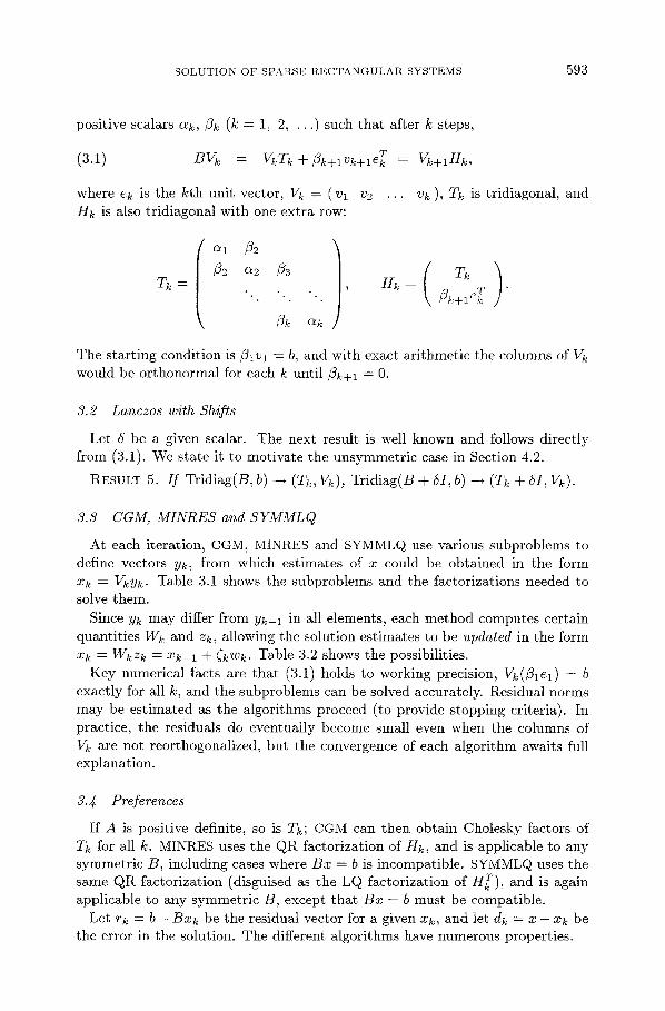
Tk -


593

positive scalars cxk, 13k (k = 1 ; 2, . . .) such that after k steps,

(3.1)

BVk = VkTk +/3k+1Vk+1ek = Vk+lHk,

where ek is the kth unit vector, Vk = (v 1 v2 . . . vk ), Tk is tridiagonal, andHk is also tridiagonal with one extra row :

/ a1 132

\02 a2 J33

TkHk =

~k+l ek

l3k ak f

The starting condition is j3 1v 1 = b, and with exact arithmetic the columns of Vkwould be orthonormal for each k until /3k+1 = 0-

3.2 Lanczos with Shifts

Let 6 be a given scalar . The next result is well known and follows directlyfrom (3.1) . We state it to motivate the unsymmetric case in Section 4 .2 .

RESULT 5 . If Tridiag(B, b) -~ (Tk, Vk), Tridiag(B + SI, b) -> (Tk + SI, Vk) .

3.3 CGM, MINRES and SYMMLQ

At each iteration, CGM, MINRES and SYMMLQ use various subproblems todefine vectors yk, from which estimates of x could be obtained in the formxk = Vkyk . Table 3 .1 shows the subproblems and the factorizations needed tosolve them .

Since Yk may differ from Yk_1 in all elements, each method computes certainquantities Wk and zk, allowing the solution estimates to be updated in the formxk = WkZk = xk_1 + (kwk . Table 3.2 shows the possibilities .Key numerical facts are that (3.1) holds to working precision, Vk(/3 1e 1 ) = b

exactly for all k, and the subproblems can be solved accurately . Residual normsmay be estimated as the algorithms proceed (to provide stopping criteria) . Inpractice, the residuals do eventually become small even when the columns ofVk are not reorthogonalized, but the convergence of each algorithm awaits fullexplanation .

3.4 Preferences

If A is positive definite, so is Tk; CGM can then obtain Cholesky factors ofTk for all k . MINRES uses the QR factorization of Hk, and is applicable to anysymmetric B, including cases where Bx = b is incompatible . SYMMLQ uses thesame QR factorization (disguised as the LQ factorization of Hk ), and is againapplicable to any symmetric B, except that Bx = b must be compatible.Let rk = b - Bxk be the residual vector for a given xk, and let dk = x - xk be

the error in the solution . The different algorithms have numerous properties .

594 M. A. SAUNDERS

Table 3.1: Subproblems defining Yk and xk = Vkyk for three algorithms .

Table 3.2: Definition of Wk and zk such that xk = Vkyk = Wkzk.

For example, the MINRES point xk solves the problem "min t' IIrk II such thatxk = Vky", so that IIrkll decreases monotonically, and there is no difficulty if thesystem is incompatible .

In contrast, SYMMLQ's point xk solves "mint IldkII such that xk = AVkt"[9, 15], so that IIdkII decreases . It also solves "mint' IlxkII such that xk = Vky andVkrk = 0", so that IjxkII increases, and the system must be compatible .

Note that SYMMLQ accumulates xk as a sequence of theoretically orthogonalsteps. The columns of Vk and Wk are not orthonormal in practice, but atleast IIwkII ~ 1 for SYMMLQ . On ill-conditioned systems, forming WkZk shouldinvolve less cancellation error than in MINRES (and perhaps even in CGM),where the columns of Wk could be very large .

Note also that f f rk II is often much larger for SYMMLQ than for the othermethods. Since the residual norms can be estimated cheaply, SYMMLQ hasprovision for transferring to the CGM point upon termination if the residual isthen smaller . Thus, if II rk+1 II < IIrk II, SYMMLQ takes a final step of the form

x+1 = xk + (k+lwk+l, where the last two items are already known. MINREScould transfer cheaply to the same CGM point if so desired .

Wk Zk Estimate of x

CGM Vk L-T LkDkZk = /31e1 xC = WkZk

MINRES VkRk 1 Qk~30

1 _rzk

xk = WkZk

SYMMLQI

Vk+iQk 0

bk+ li /

Lkzk = Nqiei xk = Wkzk

Method Subproblem Factorization Estimate of x

CGM Tkyk = B1e1 Tk = L kD k Lk xk = Vkyk

MINRES

SYMMLQ

min 11 Hkyk - Rlel11

min ~IYk+1II

QkHk = RO

HkQk _ (Lk 0)

xk = Vkyk

xk = Vk+lyk+1

s.t . Hkyk+l = 0lel

4 Iterative Methods for Rectangular Systems .

The preceding thoughts carry over to the methods we are interested in forsolving problems (1 .2)-(1 .4) . As described in [21, 22], LSQR and CRAIG arebased on the Golub-Kahan bidiagonalization procedure [11], which we shouldnow call a process .

4.1 The Golub-Kahan Process

Let Bidiag(A, b) -* (Bk, Uk+1 i Vk) or (Lk, Uk, Vk) denote the following process .Given a general matrix A and a starting vector b, the Golub-Kahan processgenerates vectors Uk, vk and positive scalars ak, /3k (k = 1, 2, . . .) such thatafter k steps,

AVk = Uk+1Bk = UkLk+/3k+luk+1 e k

ATUk+1 - VkBk + ak+lvk+lekk+l - Vk+IL +1,

where Uk = ( u1 u2 . . . Uk ), Vk = ( v1 V2

vk ), Lk is lower bidiagonal,and Bk is also bidiagonal with one extra row :

Lk =

The starting condition is 31 u 1 = b, and with exact arithmetic the columns of Ukand Vk would be orthonormal for each k until ak+1 = 0 or /3k+1 = 0-

4.2 Golub-Kahan with Regularization

Let S be a given scalar (> 0 without loss of generality), and define

(4.2)

AA =

6I


595

/ a1

1032 a2

A ak j

During Bidiag(A, b), orthogonal matricesplane rotations to form the quantities

k(B1)=(BOk)'

,

Qk

Bk =

Lk

0k+1ek

A=(A SI) .

may be constructed from 2k - 1

(Uk+l Yk) =(

Uk+1

where Bk (like Bk) is lower bidiagonal with dimensions (k + 1) x k . Alternatively,orthogonal matrices Qk may be constructed from 2k - 1 plane rotations to form

T

Vk

T(Lk SI )Q = (Lk 0),

(Vk Yk ) =

Uk Qk ,

596

M. A. SAUNDERS

where Lk (like Lk) is lower bidiagonal and k x k . The following results areobtained straightforwardly from (4.1)-(4 .4) .

RESULT 6 . If Bidiag(A, b) -3 (Bk, Uk+1, Vk), Bidiag(A, b) -* (Bk, Uk+1, Vk) .RESULT 7 . If Bidiag(A, b) - (Lk , Uk, Vk), Bidiag(A, b) -> (Lk, Uk, Vk)

In short, the bidiagonalizations of A = ( A) and A = (A 61) may be obtained81efficiently from the bidiagonalization of A itself . The mechanism is less trivialthan in the symmetric case. It motivates the subproblems used next .

/F.3 LSQR and CRAIG

As in the symmetric algorithms, LSQR and CRAIG use certain subproblemsto define vectors Yk and solution estimates xk = Vkyk . Table 4.1 shows thesubproblems and the factorizations needed to solve them. Table 4 .2 shows howthe factorizations are used to obtain updatable estimates xk = Wkzk .Note that Bidiag(A, b) is used in all cases . The subproblem that allows LSQR

to incorporate regularization was first proposed by Bjorck [3] . Result 6 helps toconfirm that the resulting algorithm is equivalent to applying the original LSQRto A and b . (Working backwards, the proof of Result 6 reveals the need for theorthogonal factorization (4.3), which in turn suggests the subproblem .)

Similarly, the subproblem that allows CRAIG to incorporate regularization wasoriginally just "written down", but Result 7 and its derivation now confirm thatthe resulting algorithm is equivalent to applying the original CRAIG to A and b .

4.4 The Extended CRAIG Algorithm

At last we have enough background to state the extended Craig-type algorithmfor solving the regularized least-squares problem (1 .3) in its equivalent form (1 .4),namely

min ~IxlJ 2 + 118112 subject to Ax + 6s = b .

At stage k of Bidiag(A, b), we solve the subproblem

(4 .5)

min JIM112 +

~ Itk112 subject to Lkyk + 6tk = /31e1,

using the LQ factorization in (4.4) :

(4 .6) (Lk 6I )QT = ( Lk 0),

LkZk = 131e1,

We then define solution estimates (xk, sk) as follows :

(Yktk

xk \1 _ Vkyk \1 _ Vk

( Vkyk \1 _

zk \1) Sk

/

Uktk/

Uk

tk/ -

6 /-V

k(4 .7

zk.

Since sk is not really needed, we use the top of half of VkZk to obtain xk =

WkZk, where Wk is defined in Table 4 .2 . Note that Yk is not needed either,but computation of Wk from Uk and Qk requires additional work and storage .(In contrast, LSQR does not need (Tk+l or Yk in (4.3), so incurs little cost withregularization .) Table 4 .3 compares the algorithms .


Table 4.1 : Subproblems defining yk and xk = Vkyk for four algorithms .

Table 4 .2 : Definition of Wk and Zk such that xk = Vkyk = Wkzk .

Table 4.3 : Comparison of algorithm costs with and without regularization .

597

Wk Zk

LSQR 6 = 0 VkRk 1 Q0161

zk=

~k+1

6 > 0 VkRk 1 Qk~Lel

} = Sk+I4k

CRAIG 6 = 0 Vk zk = yk

6 > 0 ( Vk 0 )Q( Ik

)k

O /Lkzk = 0lel

Method Subproblem Factorization

LSQR

6 = 0 min Bkyk - 01e11QkBkRk

=C )

0

6 > 0 minBk

~1 el Bk

-Rk

QkSI yk

0/

/061

0

CRAIG 6 = 0

6>0

Lkyk = /31e1

min Iyk112+ It k ll2 (Lk 6I)Qk =(Lk 0)

s .t . Lkyk + Stk = 131e1

Storage Work per iteration

LSQR, any 6CRAIG, 6 = 0CRAIG, 6 > 0

m + 3nm + 2nm + 3n

3m + 5n3m + 4n3m + 8n

598

M . A. SAUNDERS

4.5 Residuals

The solution of (4.5) satisfies

(4.10)

min

(4.11)

min

(

61

Lk

tk

eLk _6I )

)( tk'yk - ( X0 1 )

From (4.1) and (4 .8), we find that

(Si

A

sk

b+?/k/k+lUk+1AT -SI

Xk

0

where rtk is the last element of yk . Since Qk is computed as a product of planerotations,

Qk = (Ql,k+lQk+2,k+1) (Q2,k+2Qk+3,k+2) . . . (Qk-1,2k-lQ2k,2k-1) Qk,2k,

we have

Ilk = ekyk - eTN( 0)

- ekQk,2k(

0 ) = Ckekzk = Ck(k,

where ck is the cosine defining Qk,2k, and bk is the last element of zk . Thus,CRAIG may terminate when ICkCk/3k+lI is suitably small . (The analogous quan-tity when S = 0 is I(k,3k+1l [21] .)

4 .6 Transferring to the LSQR Point

Just as (1.4) is equivalent to (1 .3) when S :?~ 0, we see that the extended CRAIGsubproblem (4.5) is equivalent to the regularized least-squares problem

2

(SI) yk- ( 30l )which is very similar to the LSQR subproblem in Table 4 .1 :

( 5 )yk -

(

/3

0

2

,

This in turn is equivalent to the minimum-length problem

(4.12)

min Ilyk11 ' + Iltk+ll12 subject to Bkyk + Stk+1 - /31e1,

which we can easily solve using the LQ factorization (4.6) already available. Afinal step from the CRAIG point to the corresponding LSQR point can thereforebe taken if desired, just as SYMMLQ can transfer to a final CGM point .

Uk+1


599

4.7 Preferences

Let rk = b - Axk be the residual for a given Xk, let dk = x - xk be the error,and first suppose that there is no regularization .LSQR chooses xk to solve the problem "min t' 1Irk!j such that xk = Vky", so

that lirk jj decreases and the system may be incompatible .The properties of CRAIG are similar to those of SYMMLQ. The CRAIG point

solves "mint 11dk11 such that xk = ATUkt" and also "min5 !Ixk 1 ! such that xk =Vky and Ukrk = 0", so that IIdkI I decreases, IlEkI I increases, and the system mustbe compatible. A benefit is that xk is formed as a sequence of orthogonal steps .

Similar properties hold when regularization is introduced . However, for CRAIGit is estimates of the combined vector (s) that are formed via orthogonal steps .We cannot expect good accuracy in the final estimate of x if jjxjj << I1s1l .

5 The Broad Picture .

For completeness we state the following results, linking the regularized LSQRand CRAIG algorithms to hypothetical ones based on the symmetric Lanczosprocess. The equivalences are algebraic, and they generalize known results forthe case S = 0 . Result 9 closes a gap in existing theory .

5.1 Equivalence to CGM on Positive Definite Systems

RESULT 8 . The LSQR iterates xk are the same as the CGM iterates xk for theproblem (ATA + 521)x = ATb .RESULT 9 . The Extended CRAIG iterates xk are related to the CGM iterates

for the problem (AAT + 62I)t = b according to xk = ATtk .

5.2 Equivalence to CGM Subproblem for Indefinite Systems

As noted in Section 2, the augmented system

= ( 61

A ) (5.1)

KS ( s ) b,

KS

AT -S , b (0 )

is of interest when S > 0. From the Golub-Kahan process (4.1) we have

Kb(

and

SI Bk

Vk

BT -SI0

T+

ek+lak+lvk+1

Uk

_ Uk

61 Lk

13k+luk+l TKS

Vk

Vk

LT-sI +

0

) ek ,

600

M. A. SAUNDERS

which are equivalent to the Lanczos process Tridiag(K5, b) -- (T2k+1, V2k+1) and

(T2k, V2k) respectively, where

/ 6 a l

T2k+1 =

and

02S a2

ak -S

,3k+1

/3k+16 1

V2k+1

u2

uk

uk+12k+1 =

V1

V2

Vk

RESULT 10 . Subproblem k in LSQR is equivalent to subproblem 2k+1 in CGMfor the indefinite system (5.1) .

RESULT 11 . Subproblem k in Extended CRAIG is equivalent to subproblem 2kin CGM for the indefinite system (5.1) .

5 .3 Alternative Implementations

The equivalence of problems (1 .3) and (1.4) reveals that there are two dis-tinct ways of solving the regularized least-squares problem, based on distinctorthogonal factorizations . We may call these two implementations :

LSl FormQ ( 61 / _

( R ), set(d ) = Q ( / ,

and solve Rx = c .

LS2 Form (A SI )QT = (L 0), solve Lz = b, and form (X) = QT( zs

0

Similarly, there are two possible implementations of LSQR (when S > 0) and twooptions for extending CRAIG, based on two ways of solving the subproblems inTable 4 .1 :

LSQR1

Use QR factors of Bj , as in the standard LSQR .

LSQR2

Use LQ factors of (Bk SI ) .

CRAIGI Use QR factors of LkSICRAIG2 Use LQ factors of (Lk SI ), as in Section 4 .4 .

Experiments with Matlab indicate that the LSQRI matrix is typically betterconditioned than the other three shown . Hence, the standard LSQR implemen-tation is probably the most reliable (and fortunately also the most efficient) .

T2k

0 /3k+1

Uk+l

0

1

l

6 Numerical Tests.

We have compared LSQR and the extended CRAIG method on a range ofregularized least-squares problems in which A has one of the forms

A=Y(o )Z,

YDZ,

or Y(D 0)Z,

where D is a diagonal matrix containing specified singular values, and Y andZ are Householder matrices. (The problems are regularized versions of those in[21] .)Figure 6.1 shows how 11A'rk - S`xk 11 and the error I1 x - xk 11 varied on a

particular under-determined problem with A reasonably ill-conditioned (m =100, n = 200, cond(A) ;~_- 106, 11A11 = 1, jIblj ~~ 1, llxI ;z,- 1, 1Iril .:: 5 x 10_4 ,

6 = 10 -6 , machine precision c : 10-16 )

The plots for LSQR seem considerably preferable at first sight, and suggest thattransferring to the LSQR point may often be desirable . Since CRAIG minimizesthe error in the combined vector (x, s), the error in x itself may not be monotonic .The effect is exaggerated by the fact that 1 s 1l = 1 r 1l 16 ti 500 >> 11 x l l .In general, CRAIG performed well on systems of all shapes if (jrlj was not

too large and 6 was not too small (say lrlJ/6 < 104) . After transfer to theLSQR point, the final solution agreed closely with LSQR . Under more extremeconditions, it was apparent that I xk Il may exceed the exact 1IxI by a large factor,and cancellation can occur during transfer to the final LSQR point . This is adefinite disadvantage .

It was observed that LSQR also performed reliably on systems of all shapes (in-cluding ones that were strongly under-determined), with no apparent restrictionon jjrjj or 6 . We checked for cancellation in the LSQR update xk = (VkRk 1 )zk =xk_1 + (kwk by monitoring (k, lwkll and their product (at no cost, since jlwkIlis already needed for one of LSQR's stopping criteria) . We found that lwkjj wasindeed often large, but the corresponding ck was invariably small. (The largestchange to xk was always for k = 1!) Thus, we have not yet found cases toillustrate CRAIG's potential advantage . Future tests on the examples proposedin [13] may be more revealing .

7 Conclusions .

Since Craig's method is efficient and reliable for compatible systems Ax = b, ithas long seemed desirable to extend it to least-squares problems . The extensiongiven here is equivalent to applying the existing method to a compatible systemAx + 6s = b. It should therefore retain good numerical properties when 11s11/IIxI1is not too large . (Thus, 11b - Ax 11 should not be very large, and 6 should not betoo small.) Incompatible under-determined systems are likely candidates .The extended method is slightly more expensive than LSQR . A potential

advantage exists on problems for which the LSQR iterates are much larger thanthe solution : 11xkjj >> 11x11 . However, we have not yet found examples of suchproblems .


601

602

5

0m00)J -5

0

-100 50

Acknowledgements .

I owe special thanks to Chris Paige for encouraging this work and for laying thefoundations long ago. His comments on the manuscript were equally valuable . Iam also grateful to Ake Bjorck, Bernd Fischer, Gene Golub and the referee fortheir kind help at critical moments.

100

M. A. SAUNDERS

150 200 250

Figure 6 .1: Residuals II ATrk - S 2xk it for normal equations (A TA + 62I)x = ATb,and corresponding errors lix - xk 11 . LSQR -, CRAIG • • . .

A benefit of this research has been to observe that LSQR's reliable performanceon over-determined systems seems to hold for under-determined systems also(with or without regularization) .A further benefit has been to focus on the augmented system (2.2) and the

fact that cond(K8) : IIA11/S, suggesting a direct method for sparse equationsand least-squares problems based on indefinite Cholesky factors (see Section 2) .

The presentation has followed Paige [19] (and [20]) in emphasizing the sepa-ration of the Lanczos and Golub-Kahan processes from the subproblems used todefine particular solution methods . It also illustrates the parallels between thealgorithms for symmetric and unsymmetric equations, and unifies the bidiago-nalizations of A, ( S7) and (A SI ) .


603

REFERENCES1. M. Arioli, I. S. Duff and P . P. M . de Rijk, On the augmented system approach to

sparse least-squares problems, Numer. Math ., 55 (1989), pp . 667-684 .2 . A. Bjorck, Iterative refinement of linear least squares solutions I, BIT, 7 (1967),

pp. 257-278 .3 . A. Bjorck, A bidiagonalization algorithm for solving ill-posed systems of linear equa-

tions, Report LITH-MAT-R-80-33, Dept . of Mathematics, Linkoping University,Linkoping, Sweden, 1980 .

4 . A. Bjorck, Pivoting and stability in the augmented system method, in D. F . Griffithsand G. A. Watson (ads .), Numerical Analysis 1991 : Proceedings of the 14th DundeeConference, Pitman Research Notes in Mathematics 260, Longman Scientific andTechnical, Harlow, Essex, 1992 .

5. J . E. Craig, The N-step iteration procedures, J. Math . and Phys ., 34, 1 (1955), pp .64-73 .

6 . A. Dax, On row relaxation methods for large constrained least-squares problems,SIAM J . Sci. Comp., 14 (1993), pp . 570-584 .

7. I . S. Duff and J. K. Reid, Exploiting zeros on the diagonal in the direct solution ofindefinite sparse symmetric linear systems, ACM Trans. Math . Softw ., to appear .

8. D. K. Faddeev and V. N. Faddeeva, Computational Methods of Linear Algebra,Freeman, London, 1963 .

9. R. W. Freund, Uber einige CG-ahnliche Verfahren zur Losung linearer Gle-ichungssysteme, Ph.D. Thesis, Universitat Wiirzburg, FRG, 1983 .

10. P. E. Gill, M. A. Saunders and J . R. Shinnerl, On the stability of Cholesky factor-ization for quasi-definite systems, SIAM J. Mat. Anal., 17(1) (1996), to appear .

11. G. H. Golub and W . Kahan, Calculating the singular values and pseudoinverse ofa matrix, SIAM J . Numer. Anal., 2 (1965), pp . 205-224 .

12. G. H. Golub and C . F. Van Loan, Unsymmetric positive definite linear systems,Linear Alg. and its Appl., 28 (1979), pp . 85-98 .

13. P. C. Hansen, Test matrices for regularization methods, SIAM J . Sci. Comput .,16(2) (1995), pp . 506-512 .

14. G. T. Herman, A . Lent and H . Hurwitz, A storage-efficient algorithm for findingthe regularized solution of a large, inconsistent system of equations, J. Inst . Math .Appl., 25 (1980), pp. 361-366 .

15. D. P. O'Leary, Private communication, 1990 .16. C. Lanczos, An iteration method for the solution of the eigenvalue problem of linear

differential and integral operators, J . Res. Nat . Bur. Standards, 45 (1950), pp . 255-282 .

17. P. Matstoms, Sparse QR factorization in MATLAB, ACM Trans . Math. Software,20(1) (1994), pp . 136-159 .

18. C. C. Paige, Bidiagonalization of matrices and solution of linear equations, SIAMJ. Numer. Anal., 11 (1974), pp . 197-209.

19. C. C. Paige, Krylov subspace processes, Krylov subspace methods and iteration poly-nomials, in J. D . Brown, M. T. Chu, D . C. Ellison, and R . J. Plemmons, eds ., Pro-ceedings of the Cornelius Lanczos International Centenary Conference, Raleigh,NC, Dec. 1993, SIAM, Philadelphia, 1994, pp . 83-92 .

20. C. C. Paige and M . A. Saunders, Solution of sparse indefinite systems of linearequations, SIAM J. Numer. Anal., 12(4) (1975), pp . 617-629 .

604

M. A. SAUNDERS

21 . C. C. Paige and M . A. Saunders, LSQR: An algorithm for sparse linear equationsand sparse least squares, ACM Trans. Math. Software, 8(1) (1982), pp. 43-71 .

22. C. C. Paige and M . A. Saunders, Algorithm 583. LSQR: Sparse linear equationsand least squares problems, ACM Trans. Math. Software, 8(2) (1982), pp. 195-209 .

23. M. A. Saunders, Cholesky-based methods for sparse least squares : The benefits ofregularization, Report SOL 95-1, Dept . of Operations Research, Stanford Univer-sity, California, USA, 1995 .

24. R. J . Vanderbei, Symmetric quasi-definite matrices, SIAM J . Optim., 5(1) (1995),pp. 100-113 .

Documents

Solution of sparse rectangular systems using LSQR and CRAIG