Embed Size (px)
Citation preview

Master of Science Thesis
KTH School of Industrial Engineering and Management
Energy Technology EGI-2015-064MSC EKV1102
Division of Heat and Power Technology
SE-100 44 STOCKHOLM
Solar PV-CSP Hybridisation for
Baseload Generation
A Techno-economic Analysis for the Chilean
Market
Kevin Larchet

ii
Master of Science Thesis EGI-2015-064MSC
EKV1102
Solar PV-CSP Hybridisation for Baseload
Generation
A Techno-economic Analysis for the Chilean
Market
Kevin Larchet
Approved
Examiner
Björn Laumert
Supervisor
Rafael Guédez
Commissioner
Contact person
Abstract
The development of high capacity factor solar power plants is an interesting topic, especially when
considering the climate and economic conditions of a location such as the Chilean Atacama Desert. The
hybridisation of solar photovoltaic (PV) and concentrating solar power (CSP) technologies for such an
application is a promising collaboration. The low cost of PV and dispatchability of CSP, integrated with
thermal energy storage (TES), has the promise of delivering baseload electricity at a lower cost than what
could be achieved with CSP alone. Therefore, the objective of this work was to evaluate whether or not a
hybrid PV-CSP plant is more economically viable, than CSP alone or hybrid PV-diesel, for baseload
generation. To analyse this hypothesis, a techno-economic optimisation study of a PV-CSP hybrid plant
with battery storage and fossil fuel backup was performed. In doing so, a methodology for the
identification of optimum solar hybrid plant configurations, given current technology and costs, to best
satisfy specific location weather and economic conditions was developed. Building on existing models, for
the PV and CSP components, and developing models for further hybridisation, a complete PV-CSP
model was created that could satisfy a baseload demand. Multi-objective optimisations were performed to
identify optimal trade-offs between conflicting technical, economic and environmental performance
indicators. For the given economic and technical assumptions, CSP hybridised with fossil fuel backup was
shown to provide electricity at the lowest cost and have the lowest project capital expenditure. This
configuration showed a 42% and 52% reduction in the levelised cost of electricity in comparison to CSP
alone and hybrid PV-diesel, respectively. It also provides a 45% reduction in CAPEX in comparison to
CSP alone. PV-CSP integration increases capital costs and the cost of electricity, but reduced the use of
fossil fuel backup and thereby reduced emissions, when compared to CSP with fossil fuel backup.
However PV-CSP showed a 97% reduction in CO2 emissions when compared to hybrid
PV-diesel. Furthermore, it showed a 35% and 46% reduction in LCOE in comparison to CSP alone and
hybrid PV-diesel.

iii
Acknowledgments
Firstly I would like to express my utmost gratitude to my supervisor, Rafael Guédez, for his support and
inspiration throughout this master thesis project. Secondly I would like to thank Björn Laumert and the
rest of the Solar Power Research Group at KTH for giving me the opportunity to work with them for
these past months. Last but not least I would like thank all my master thesis colleagues and friends at
KTH for the support and the good times that were had during this intense but thoroughly enjoyable
period.

iv
Nomenclature
Abbreviations
AC Alternating Current
AHI Aqueous Hybrid Ion
a-Si Amorphous Silicon
BESS Battery Energy Storage System
BOP Balance of Plant
BOS Balance of Systems
C Condenser
Cont Contingency
Conv Converter
CPV Concentrating Solar PV
c-Si Crystalline Silicon
CSP Concentrating Solar Power
D Deaerator
DC Direct Current
DHI Diffuse Horizontal Irradiance
DNI Direct Normal Irradiance
DOD Depth of Discharge
DR Discount Rate
DYESOPT Dynamic Energy System Optimizer
E&C Engineering and Construction
EC Economiser
EOH Equivalent Operating Hours
EPC Engineering, Procurement and Construction
EV Evaporator
FC Fuel Consumption
FiT Feed-In Tariff
GB Gas Boiler
Genset Generator Set
GHI Global Horizontal Irradiance
HPT High Pressure Turbine
HTF Heat Transfer Fluid
HTL Hot Tank Level
Instal Installation
Inv Inverter
ISCC Integrated Solar Combined Cycle
LCOE Levelised Cost of Electricity
Li-Ion Lithium-Ion
Li-NMC Lithium Nickel Manganese Cobalt Oxide
LPT Low Pressure Turbine
LTO Lithium Titanate

v
MATLAB Matrix Laboratory
Misc Miscellaneous
MPP Maximum Power Point
MPPT Maximum Power Point Tracker
m-Si Monocrystalline Silicon
NG Natural Gas
NOCT Normal Operating Cell Temperature
NOH Normal Operating Hours
OCV Open Circuit Voltage
OM Operating Mode
OPEX Operating Expenditure
PB Power Block
PCS Power Conditioning System
PID Proportional Integral Derivative Controller
PLR Part Load Ratio
PLR Power Purchasing.Agreement
p-Si Polycrystalline Silicon
PV Photovoltaic
Ref Reference
RH Reheater
RSC Reference Site Data
SDR Degradation Factor
Serv Services
SEGS Solar Energy Generating Systems
SH Superheater
SF Solar Field
SING Sistema Interconectado del Norte Grande
SM Solar Multiple
SOC State of Charge
Soft Soft Costs
STC Standard Testing Conditions
STPP Solar Tower Power Plant
TES Thermal Energy Storage
TF Thin Film
TMY Typical Meteorlogical Year
TRNSYS Transient Systems Simulation Program

vi
Symbols
C Cost [$]
eqc OCV on charge [V]
eqd OCV on discharge [V]
F State of charge [-]
FCNG Fuelc consumption of NG [kg]
FCDG Fuel comsumption of diesel [kg]
gc Fractional SOC coefficient on charge [-]
gd Fractional SOC coefficient on discharge [-]
H Fractional SOC [-]
I Current [A]
IMPP MPP current [A]
Isc Short circuit current [A]
Iq max Charge current limit [A]
Iq min Discharge current limit [A]
mc Cell type parameter on charge [-]
md Cell type parameter on discharge [-]
Qc Capacity parameter on charge [-]
Qd Capacity parameter on discharge [-]
Qm Cell rated capacity [Ah]
Q Heat energy [W]
rqc Internal resistance on charge [Ω]
rqd Internal resistance on discharge [Ω]
V Voltage [V]
Vc Charge voltage limit [V]
Vd Discharge voltage limit [V]
VMPP MPP voltage [V]
Voc Open circuit voltage [V]
W Power [W]
η Efficiency [%]

vii
Table of Contents
Abstract ........................................................................................................................................................................... ii
Acknowledgments ........................................................................................................................................................ iii
Nomenclature ............................................................................................................................................................... iv
Abbreviations ........................................................................................................................................................... iv
Symbols ..................................................................................................................................................................... vi
Table of Contents ........................................................................................................................................................ vii
List of Figures ............................................................................................................................................................... ix
List of Tables................................................................................................................................................................. xi
1 Introduction .......................................................................................................................................................... 1
1.1 Previous Works ........................................................................................................................................... 2
1.2 Objectives ..................................................................................................................................................... 2
2 Literature Review ................................................................................................................................................. 3
2.1 Solar Energy ................................................................................................................................................. 3
2.1.1 Solar Energy Technologies ............................................................................................................... 4
2.1.2 Standard Terminology ....................................................................................................................... 4
2.2 Solar Photovoltaics ..................................................................................................................................... 6
2.2.1 Operation ............................................................................................................................................ 6
2.2.2 Intermittency ...................................................................................................................................... 6
2.2.3 PV Cell Types ..................................................................................................................................... 7
2.2.4 Performance ........................................................................................................................................ 7
2.2.5 PV Plant Configurations .................................................................................................................11
2.2.6 Electrical Energy Storage ................................................................................................................14
2.3 Concentrating Solar Power ......................................................................................................................19
2.3.1 Operation ..........................................................................................................................................19
2.3.2 CSP Plant Types ...............................................................................................................................19
2.3.3 Solar Field .........................................................................................................................................20
2.3.4 Thermal Energy Storage & Dispatchability .................................................................................21
2.3.5 Power Block ......................................................................................................................................22
2.3.6 Hybridisation & Backup .................................................................................................................23
2.4 Hybrid Solar PV & CSP ...........................................................................................................................25
2.4.2 Baseload Solar ...................................................................................................................................27
2.4.3 Current Projects ...............................................................................................................................27
2.5 Market: Chile ..............................................................................................................................................29
3 Methodology ....................................................................................................................................................... 31
3.1 DYESOPT .................................................................................................................................................31
3.2 Model Description & Steady State Design ...........................................................................................32
viii
3.2.1 CSP Model ........................................................................................................................................32
3.2.2 PV Model ..........................................................................................................................................33
3.2.3 Battery Model ...................................................................................................................................33
3.2.4 Boiler Model .....................................................................................................................................37
3.3 Combined Model ......................................................................................................................................38
3.3.1 Dispatch Strategy .............................................................................................................................40
3.3.2 Operating Modes .............................................................................................................................41
3.3.3 Dynamic Model ................................................................................................................................44
3.3.4 Techno-economic Calculations .....................................................................................................45
3.4 Model Verification ....................................................................................................................................48
3.4.1 STPP Model ......................................................................................................................................48
3.4.2 PV Plant Model ................................................................................................................................48
3.4.3 PV-CSP Model .................................................................................................................................49
3.5 Multi-Objective Optimisation .................................................................................................................50
3.5.1 Design Variables and Objectives ...................................................................................................51
4 Results .................................................................................................................................................................. 52
4.1 Case 1: Minimise LCOE and CAPEX...................................................................................................52
4.1.1 Single Capacity Case ........................................................................................................................55
4.2 Case 2: Minimise CO2 emissions and LCOE .......................................................................................56
4.2.1 Single Capacity Case ........................................................................................................................58
4.3 Dynamic Performance .............................................................................................................................61
4.4 Comparison with Competing Technologies .........................................................................................67
5 Discussion ........................................................................................................................................................... 69
6 Conclusions ......................................................................................................................................................... 71
6.1 Future Work ...............................................................................................................................................72
Bibliography ................................................................................................................................................................. 73
ix
List of Figures
Figure 1: Solar potential compared to other renewable sources [11] .................................................................... 3
Figure 2: Share of primary energy sources in world electricity generation mix 2008 [12] ................................. 4
Figure 3: Solar energy technologies [11] [13] ............................................................................................................ 4
Figure 4: Load curve definitions [15] ......................................................................................................................... 5
Figure 5: Operation of a PV cell [12] ......................................................................................................................... 6
Figure 6: PV power output intermittency [18] .......................................................................................................... 7
Figure 7: I-V curve and MMP [5] ............................................................................................................................... 8
Figure 8: I-V curve with varying solar irradiance [22] ............................................................................................. 8
Figure 9: I-V curve with varying temperature [22] ................................................................................................... 9
Figure 10: Addition of PV modules and strings to create arrays [5] ..................................................................... 9
Figure 11: Effect of partial shading on PV string I-V curve [10] ........................................................................10
Figure 12: Centralised PV configuration [29] .........................................................................................................11
Figure 13: String inverter configuration [29] ...........................................................................................................12
Figure 14: Multi-string inverter configuration [29] ................................................................................................12
Figure 15: Module inverter configuration [30]........................................................................................................13
Figure 16: AC coupling of BESS to centralized inverter PV plant .....................................................................17
Figure 17: DC coupling of BESS to multi-string inverter PV plant ...................................................................18
Figure 18: Single stage inverter/charge controller system [55] ............................................................................18
Figure 19: Main types of CSP plant [2] ....................................................................................................................19
Figure 20: Simplified CSP plant configuration [10] ...............................................................................................20
Figure 21: CSP dispatchability [4] .............................................................................................................................22
Figure 22: STPP reheat Rankine power block [66] ................................................................................................23
Figure 23: Utilisation of backup boiler [71] ............................................................................................................24
Figure 24: Back up boiler integrated into steam cycle ...........................................................................................24
Figure 25: PV-CSP rendering [75] ............................................................................................................................25
Figure 26: PV-CSP schematic [50] ............................................................................................................................25
Figure 27: Typical weekly operation of a PV-CSP plant with backup ................................................................26
Figure 28: Global DNI map [88] ..............................................................................................................................29
Figure 29: Installed capacity of SING 2015 [92] ....................................................................................................30
Figure 30: DYESOPT flow chart [93] .....................................................................................................................31
Figure 31: Rankine Cycle design flowchart .............................................................................................................32
Figure 32: HTF cycle flowchart ................................................................................................................................32
Figure 33: Field growth method in hybrid algorithm (Adapted from [99]) .......................................................32
Figure 34: BESS model validation discharge curve ...............................................................................................36
Figure 35: BESS model validation charge curve ....................................................................................................36
Figure 36: Boiler efficiency curve based on feedwater mass flowrate [71] ........................................................37
Figure 37: Annual DNI at Calama ............................................................................................................................39
Figure 38: Daily SING generation curve [113] .......................................................................................................39
Figure 39: Daily operation with dispatch strategy 1 and 2 ....................................................................................40
Figure 40: Dispatch strategy flow chart ...................................................................................................................41
Figure 41: Operating modes of hybrid PV-CSP plant...........................................................................................42
Figure 42: PID controller tuning [116] ....................................................................................................................45
Figure 43: Pareto curve illustration [129] ................................................................................................................50
Figure 44: Case 1 plant capacity results ...................................................................................................................52
Figure 45: Case 1 share of electricity generation results........................................................................................53
Figure 46: Case 1 solar muliple and TES results ....................................................................................................53
Figure 47: Case 1 NG consumption and OPEX results .......................................................................................54
Figure 48: Case 1 seasonal load results ....................................................................................................................54
Figure 49: Case 1 fixed capacity plant capacity results ..........................................................................................55

x
Figure 50: Case 1 fixed capacity share of electricity generation results ..............................................................55
Figure 51: Case 2 plant capacity results ..................................................................................................................56
Figure 52: Case 2 share of electricity generation results........................................................................................57
Figure 53: Case 2 seasonal load results ....................................................................................................................58
Figure 54: Case 2 CAPEX results .............................................................................................................................58
Figure 55: Case 2 fixed capacity plant capacity results ..........................................................................................59
Figure 56: Case 2 fixed capacity share of electricity generation results ..............................................................60
Figure 57: Case 2 fixed capacity CAPEX results ....................................................................................................60
Figure 58: Dynamic performance plant configurations ........................................................................................61
Figure 59: Week operation of Plant A1 ....................................................................................................................63
Figure 60: Week operation of Plant A2 ....................................................................................................................63
Figure 61: CAPEX and OPEX breakdown of plant A1 and A2 ..........................................................................64
Figure 62: Week operation of Plant B1 ....................................................................................................................65
Figure 63: Week operation of Plant B2 ....................................................................................................................66
Figure 64: CAPEX and OPEX breakdown of plant B1 and B2 ...........................................................................66

xi
List of Tables
Table 1: Advantages and disadvantages of PV inverter configurations [31]......................................................13
Table 2: Functions of BESS [38] ..............................................................................................................................14
Table 3: Battery technologies ....................................................................................................................................15
Table 4: Advantages and disadvantages of NG and diesel backup .....................................................................24
Table 5: Technical data for a planned PV-CSP plant in Copiapó .......................................................................28
Table 6: Technical data for the Atacama 1 and Atacama 2 PV-CSP plants ......................................................28
Table 7: Technical data for Redstone PV-CSP plant.............................................................................................29
Table 8: Important parameter definitions ...............................................................................................................34
Table 9: Battery model input parameters ................................................................................................................35
Table 10: Calama TMY data ......................................................................................................................................38
Table 11: Simulation RSC data ..................................................................................................................................38
Table 12: Operating modes of hybrid PV-CSP plant ............................................................................................43
Table 13: PID controller parameters ........................................................................................................................44
Table 14: STPP model design parameters ...............................................................................................................48
Table 15: STPP dynamic performance ....................................................................................................................48
Table 16: PV plant design parameters......................................................................................................................49
Table 17: PV plant dynamic performance ...............................................................................................................49
Table 18: PV-CSP plant dynamic performance ......................................................................................................49
Table 19: Multi-objective optimisation design variables .......................................................................................51
Table 20: Multi-objective optimisation design objectives .....................................................................................51
Table 21: Point A design parameters and performance indicators .....................................................................62
Table 22: Point B design parameters and performance indicators ......................................................................65
Table 23: Comparison on different cases and plant configurations ....................................................................67
Table 24: Model LCOE and real case PPA comparison .......................................................................................70

1
1 Introduction
The share of renewable energy technologies in the global energy mix has been steadily increasing,
particularly with regards to the energy sector [1]. The causes of this trend are numerous and can be mainly
attributed to several global challenges [2]. These challenges, which include the need of alternative sources
of energy, climate change and sustainable development, have been stimulating technological advancements
in the energy sector. However, if goals of reducing CO2 emissions are to be realised, these clean energy
technological developments must be accelerated [2].
One of the most promising sources for the generation of clean energy is solar energy. Solar energy is the
most abundant energy resource on the planet, with approximately 885 million TWh of energy reaching the
planet surface every year [2]. This staggering value completely dwarfs the annual energy consumption of
the human population, which was approximately 104,426 TWh in 2012 [3]. In other words, it takes the
sun 85 minutes to provide the earth with the amount of energy that it consumes in a year [4]. For the
same amount of energy to reach land only it would take little more than 4 hours 30 minutes [4]. There are
two main types of solar energy technologies that can harvest this abundant energy resource; solar
photovoltaics (PV) and concentrating solar power (CSP).
PV converts solar energy directly into electricity, through the photovoltaic process, and is one of the
fastest growing renewable energy technologies in the world today with more PV capacity added since 2010
than in the last four decades [5] [6]. Due to this, it expected to play a major role in the future global energy
mix. Solar PV modules are cheap, small and highly modular and can be used virtually anywhere [5].
However, one of the main characteristics of solar PV, and one of its main disadvantages, is that it is a
highly intermittent form of energy generation. This characteristic can cause issues regarding grid
integration and power supply stability. Storage can add a dimension of dispatchability but currently it is
too costly to be implemented at a large scale [6].
CSP converts solar energy into electricity through a thermoelectric process. CSP is also an intermittent
form of generation but has the added value of dispatchability when combined with thermal energy
storage (TES) [4]. TES is a cost effective way of decoupling the electrical output of a CSP plant from the
solar input, i.e. its reliance on the instantaneous solar irradiance [7]. Cost effective dispatchability gives
CSP a clear technological advantage over solar PV and other intermittent renewable energy technologies
and this has made CSP a very interesting technology for future sustainable energy generation.
The topic of this thesis is the hybridisation of solar PV and CSP technologies which otherwise would be
in competition with each other. The combination of low cost PV and dispatchable CSP makes a
promising collaboration from an economic point of view and is currently gaining some attention with one
hybrid project currently in development. The reduction of solar power plant costs is important in order
for these technologies to gain competitive advantage against traditional fossil fuel generation. Therefore
the topic of this thesis is the examination of the economic viability of combining these technologies for
baseload operation through techno-economic means.

2
1.1 Previous Works
1. “High Capacity Factor CSP-PV Hybrid Systems, 2015”, by Green, et al., 2015.
In this study, the performance of a high capacity factor PV-CSP plant was examined in Chile. The hourly
performance of the plant was evaluated through the use of SolarReserve’s SmartDispatch software. Using
this software, priority levels of plant power output were assigned. Annual simulations were carried out for
both a PV-CSP hybrid plant and a standard CSP plant. While this study performs analysis on hybrid
PV-CSP plants from a technical aspect, it neglects any form of economic analysis [8].
2. “Thermo-economic Evaluation of Solar Thermal and Photovoltaic Hybridisation Options
for Combined-cycle Power Plants”, by Spelling and Laumert, 2015.
In this study, the performance of CSP and solar PV hybridisation of combined-cycle plants were analysed
at a distribution level. The analysed hybrid plant configurations include solar PV combined-cycle plants,
integrated solar combined-cycle plants and hybrid gas turbine combined-cycle plants. Their performance
were analysed from a technical, economic and environmental aspect. While this study focuses on solar
energy hybridisation, it does not consider the hybridisation of CSP and PV [9].
3. “Techno-economic Analysis of Combined Hybrid Concentrating Solar and Photovoltaic
Power Plants: A Case Study for Optimizing Solar Energy Integration into the South
African Electricity Grid”, by Castillo, 2014.
This study, a previous master thesis project, focused on the analysis of hybrid PV-CSP systems for peak
load. It evaluated the feasibility of these hybrid plants, for the particular case of South Africa, and analysed
plant performance through techno-economic means. However, it did not consider the hybrid plant for
baseload operation. Furthermore a sensitivity analysis was conducted rather than a full optimisation [10].
To summarise, no previous works performed optimisation studies, whilst coupling the analysis of
detailed economics with technical aspects, for the design of hybrid PV-CSP plants for baseload
operation. In doing so, a methodology for the identification of optimum solar hybrid plant
configurations, given current technology and cost development, to best satisfy specific location
weather and economic conditions has been developed.
1.2 Objectives
The main objective of this thesis is to determine, for a specific location, whether or not a hybrid solar
PV-CSP power plant is more economical viable for baseload operation than CSP alone or PV-diesel
genset hybrid. In order to prove this hypothesis, some specific objectives must be accomplished.
Conduct a detailed and thorough literature review which includes theoretical background into the
technologies, the hybridisation of the technologies, potential markets and techno-economic
performance modelling.
Acquaintance of existing models and coupled PV-CSP hybrid model. This includes the validation
of PV and CSP models and the verification of the coupled model against known projects
Development and validation of hybridisation models to ensure baseload operation. This also
includes the implementation of hybrid plant coupling strategies and the dispatch strategy.
Perform a techno-economic study to analyse performance of a PV-CSP plant for a given location.
This is accomplished through multi-objective optimisation using key techno-economic
performance indicators as design objectives.
Other sub objectives include:
The investigation into the viability of large scale battery storage for solar power plants.

3
2 Literature Review
This section is a detailed summary of the extensive literature review conducted in the early stages of the
thesis. This study provides much of the theoretical framework behind the work which is important in
order to get a full understanding of the various aspects of the thesis. Firstly, the technologies involved are
discussed in great detail including their advantages and disadvantages. Secondly, the advantages and
disadvantages of combining the two technologies are discussed. A detailed investigation into the need of
further hybridisation, to ensure baseload is achieved, is summarised including methods of doing so. Finally
a suitable market is defined as well as reason it was chosen.
2.1 Solar Energy
As was mentioned in Chapter 1, solar energy is the most abundant energy resource in the world today and
is very promising for future of clean energy generation [4]. The staggering statistic that it takes the sun a
little over an hour to provide the earth with the amount of energy that the human race consumes annually
is testament to that. To further illustrate this resource potential, Figure 1 visualises the solar energy
potential in comparison to other energy sources available and the annual global energy consumption.
Figure 1: Solar potential compared to other renewable sources [11]
According to the International Energy Agency, 2011, the estimated reserves of oil, natural gas and coal are
46 years, 58 years and 150 years respectively [4]. These values are estimated from proven fuel reserves and
consumption at current rates. In the same sense, if the entire annual solar potential was harvested and
stored, it would represent over 6,000 years [4] Regardless of this potential, solar energy only accounts for a
tiny portion of the global energy mix. Even among other renewable energy sources, such as biomass,
hydro power and wind power, energy generated from solar energy is incredibly small. This is illustrated by
Figure 2, which describes the share of energy sources utilised for electricity generation in 2013. There are a
number of reasons why the full potential of solar energy has not been realised. The main reason is the
high cost related to the technologies. For the most part, support incentives from governments are
required in order for solar power to be competitive with conventional power generation [4].
4
Figure 2: Share of primary energy sources in world electricity generation mix 2013 [12]
2.1.1 Solar Energy Technologies
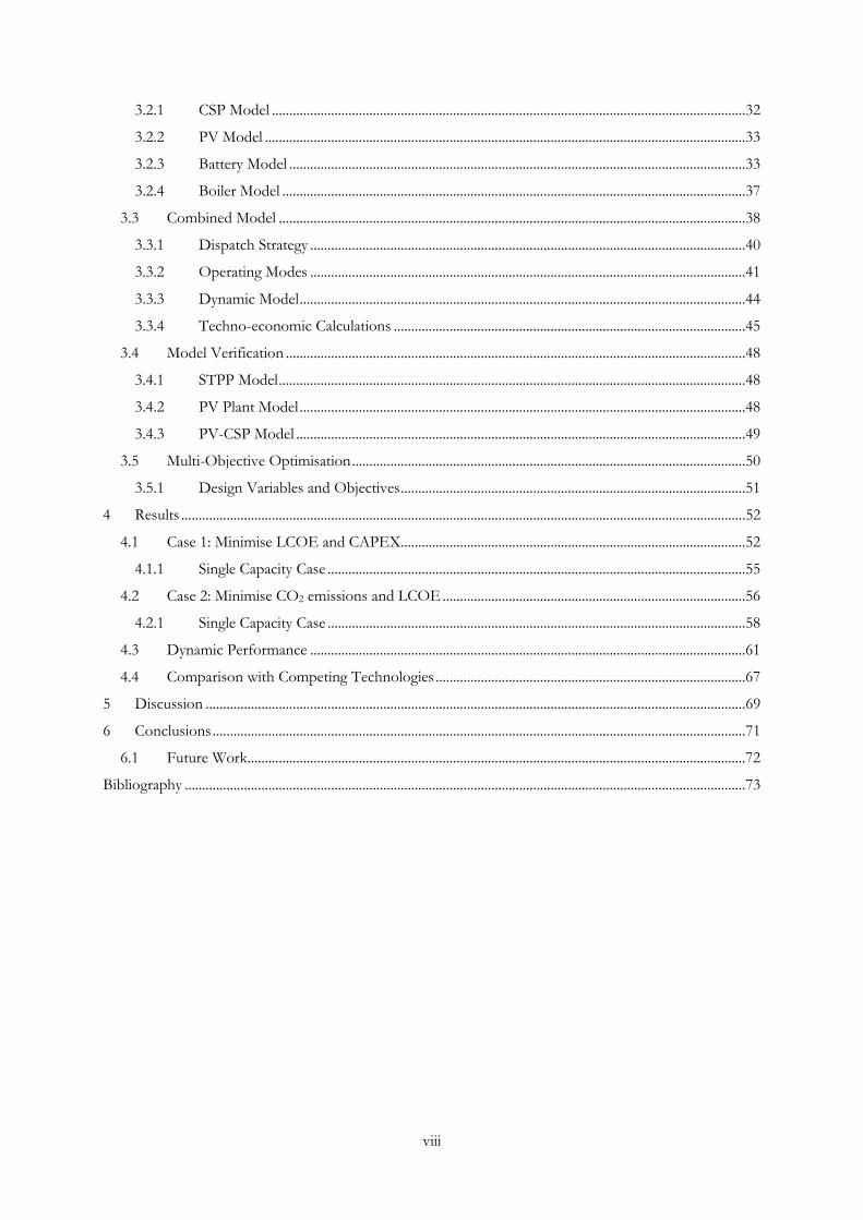
There are two main solar energy technologies currently available. These technologies operate from two
different fundamental methods of harvesting solar energy: heat and photoreaction [4]. Both technologies
cover a wide range of potential applications, ranging from domestic water heating to utility scale electricity
production. The two technologies, solar PV and CSP, are shown in Figure 3 below.
Figure 3: Solar energy technologies [11] [13]
2.1.2 Standard Terminology
The following section is a brief summary of common terminology utilised in the field of solar energy and
that are used in further discussions in this report.
Global Horizontal Irradiance
Global horizontal irradiance (GHI) is a measure of the quantity of available solar radiation per horizontal
surface area [4] [5]. It is defined as the sum of the direct normal irradiance (DNI) and diffuse horizontal
irradiance (DHI). The global irradiance can also be defined for different tilt angles which is necessary
when analysing the incoming solar radiation on solar PV modules.

5
Direct Normal Irradiance
Direct normal irradiance (DNI), also known as direct beam radiation, is a component of GHI. It is a
measure of beam irradiance per surface area and is defined as the solar radiation received on a
perpendicular surface from a narrow solid-angle [5]. This component can be maximised when the surface
is normal to the solar radiation, i.e. when single-axis or dual-axis tracking is utilised.
Diffuse Horizontal Irradiance
Diffuse horizontal irradiance (DHI) is also a component of GHI. It is defined as the amount of solar
irradiance, scattered by the atmosphere, received on a horizontal surface on the earth [5]. This includes
ground reflected radiation.
Peaking Load
Peak load refers to a period during the day where the electrical demand is significantly higher than the
average. These peaks can occur daily, monthly or even seasonally. Figure 4 illustrates peak load along with
the other load definitions. Technologies such as gas turbines and hydro are capable of covering these peak
periods due to their fast start-up [14].
Intermediate Load
The intermediate load is the load band in between the expected demand and the baseload. It usually is
characterised by periods of slow power variations [14].
Baseload
Baseload is the minimum level of demand on an electrical supply system over 24 hours. It is characterised
by plants operating continuously at very high capacity factors. These types of plants can usually produce
electricity at a lower cost than other production facilities available to the system. Examples of
conventional baseload plants are nuclear, coal, hydro amongst others [14].
Figure 4: Load curve definitions [15]

6
2.2 Solar Photovoltaics
Solar PV is the most cost effective solar energy technology on the market with prices drastically
decreasing in recent years [6]. According to the IEA, 2014, the levelised cost of electricity of PV systems
are below retail electricity prices in many countries and are rapidly approaching the level of generation
costs of traditional sources. Moreover, the technology is highly scalable and modular and so can be utilised
virtually anywhere [16]. This has made the technology incredibly fast growing with a current global
capacity of approximately 150 GW and its global share of electricity generation is predicted to reach 16%
by 2050 as opposed to 0.06% in 2008 [6] [17]. For this vision to be achieved, 4,600 GW of installed PV
capacity must be realised, which can result in an emissions avoidance of up to 4 Gt CO2 annually [6].
2.2.1 Operation
Solar PV utilises GHI to convert solar energy into electricity through the photovoltaic effect. When a
photon makes contact with a PV material, it can be absorbed, transmitted or reflected. If absorption
occurs and if the energy of the photon is greater than the band gap of the semiconductor, an electron is
released and removed through the aid of the p-n junction of the material. The electron is then free to flow
as current due to the electric field created between the n-type and p-type semiconductors [5]. The
operation of a PV cell is shown below in Figure 5.
Figure 5: Operation of a PV cell [17]
2.2.2 Intermittency
One of the main characteristics of PV electricity generation is what is known as intermittency.
Intermittency is a term to describe the variability in output of a power system due to a factor outside of
direct control. In other words, the output of a solar PV system is directly related to the amount of solar
irradiance at one given moment for a given location [6]. This characteristic could be mitigated through the
use of storage but currently large scale electrical energy storage for PV is too costly [18]. The reason for
this and a description of electrical energy storage technologies is presented in Chapter 2.2.6. The concept
of intermittency is visually represented by Figure 6, which shows the power output of a small PV farm
over three separate days. Day 3 is a normal day with a smooth output curve but day 1 and day 2 show
increased output variance. This is due to cloud cover that shade the PV array from incoming solar
radiation, decreasing the power output of the system.

7
Figure 6: PV power output intermittency [19]
2.2.3 PV Cell Types
The two main types of solar PV cells are crystalline silicon (c-Si) and thin film (TF). C-Si cells currently
dominate the market with a share of approximately 90%, while TF is represented by approximately 10%
of the market [6]. A third type called concentrating solar PV (CPV) exists but only accounts for less than
1% of the market share [6]. C-Si PV cells can be separated in monocrystalline (m-Si) and polycrystalline
cells (p-Si). In m-Si cells, the silicon comes in the form of a single crystal, without impurities. The main
advantage of this single crystal structure is that it achieves high efficiencies, typically about 14%-15% but
can also reach up to 24% [5]. However, these cells have a complicated manufacturing process resulting in
higher costs. P-Si cells consist of numerous grains of single crystal silicon and are less expensive to
manufacture but have efficiencies slightly lower than m-Si, typically of approximately 13%-15%. One
major disadvantage of c-Si cells is that their performance decreases with an increase in cell temperature, a
topic that will be covered in the next section. As such c-Si modules perform better in winter than summer
whilst the opposite can be said for amorphous silicon (a-Si) PV cells [20]. A-Si cells are arranged in a
thin homogeneous layer due to the fact that a-Si absorbs light more effectively. These PV cells have lower
manufacturing costs and are less affected by cell temperature [5]. However they operate with lower
efficiencies, of approximately 6%-7% [5].
2.2.4 Performance
The performance of a PV cell can be visualised with an I-V curve, as shown by Figure 7. The rated
performance of a PV module under specified conditions is usually represented by standard testing
conditions (STC) or normal operating cell temperature (NOCT) values provided by the manufacturer.
STC is defined as PV testing under standard conditions; an irradiance of 1000 W/m2 under cell
temperature conditions of 25 °C and assuming an airmass of 1.5.1. NOCT is a test that more closely
resembles real world conditions. In this case the solar irradiance is assumed to be 800 W/m2, an ambient
temperature is assumed to be 20 °C and an average wind speed of 1 m/s is assumed with the back of the
solar panel open to a breeze [21]. The performance of a PV module outside of rated conditions can be
calculated using temperature correction coefficients provided by the manufacturer [22].
1 Airmass is the optical path length through the Earth's atmosphere for light where the airmass at the equator is 1

8
If a PV cell is short circuited, the resulting current is at a maximum, also known as the short circuit
current (Isc) [5]. If a PV cell is open-circuited, the resulting voltage is at a maximum, also known as the
open circuit voltage (Voc). The power output of the cell, the product of the cell voltage and current, is
greater than zero between these two maximum values. The maximum power output that the cell can
achieve is called the maximum power point (MPP) and is the product of Impp and Vmpp, as shown in
Figure 7. In order to obtain the MPP a maximum power point tracker (MPPT) must be utilised. MPPTs
regulate and optimise the operating voltage of the module in order to maximise the module current and is
usually located in the inverter [5]. They can also be implemented at a string or module level, which can
have benefits in the overall performance of the array.
Figure 7: I-V curve and MMP [5]
There are two main parameters that affect the performance and MPP of a PV module.
Solar irradiance
Module temperature
Figure 8 describes the affect solar irradiance has on the performance of a PV module. It shows that, for a
fixed module temperature, the output current of the PV module increases proportionally with the solar
irradiance [23] [5]. For a fixed solar irradiance, the output voltage shows a decreasing trend with an
increase in module temperature, which is directly dependant on the ambient conditions [23] [5]. The VMPP
area represents the area at which the maximum power point voltage lies. Since a change in solar irradiance
has limited influence on the voltage, the MPP is primarily dependent on the module temperature [23].
Figure 8: I-V curve with varying solar irradiance [23]
9
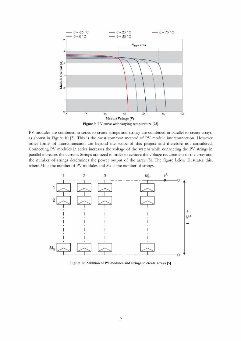
Figure 9: I-V curve with varying temperature [23]
PV modules are combined in series to create strings and strings are combined in parallel to create arrays,
as shown in Figure 10 [5]. This is the most common method of PV module interconnection. However
other forms of interconnection are beyond the scope of this project and therefore not considered.
Connecting PV modules in series increases the voltage of the system while connecting the PV strings in
parallel increases the current. Strings are sized in order to achieve the voltage requirement of the array and
the number of strings determines the power output of the array [5]. The figure below illustrates this,
where MS is the number of PV modules and MP is the number of strings.
Figure 10: Addition of PV modules and strings to create arrays [5]
10
2.2.4.1 Partial Shading & Soiling
One of the ways in which solar irradiance is reduced is through shading or soiling. Shading is the process
whereby clouds, trees, buildings or even other PV panels shade or partially shade a PV panel. This can
result in different I-V curves for both the shaded and non-shaded cells in the panel, creating a current
mismatch. Since cells are connected in series, this current mismatch can lead to cell damage and reduced
performance [24]. Cell damage comes in the form of hot spots which occur because the operating current
of a module is larger than the reduced short-circuit current of the shaded cell [25]. In terms of
performance, in order for a cell to allow the string current through it must operate in reserve bias,
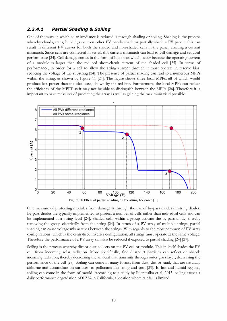
reducing the voltage of the substring [24]. The presence of partial shading can lead to a numerous MPPs
within the string, as shown by Figure 11 [24]. The figure shows three local MPPs, all of which would
produce less power than the ideal case, shown by the red line. Furthermore, the local MPPs can reduce
the efficiency of the MPPT as it may not be able to distinguish between the MPPs [26]. Therefore it is
important to have measures of protecting the array as well as gaining the maximum yield possible.
.
Figure 11: Effect of partial shading on PV string I-V curve [10]
One measure of protecting modules from damage is through the use of by-pass diodes or string diodes.
By-pass diodes are typically implemented to protect a number of cells rather than individual cells and can
be implemented at a string level [24]. Shaded cells within a group activate the by-pass diode, thereby
removing the group electrically from the string [24]. In terms of a PV array of multiple strings, partial
shading can cause voltage mismatches between the strings. With regards to the most common of PV array
configurations, which is the centralised inverter configuration, all strings must operate at the same voltage.
Therefore the performance of a PV array can also be reduced if exposed to partial shading [24] [27].
Soiling is the process whereby dirt or dust collects on the PV cell or module. This in itself shades the PV
cell from incoming solar radiation. More specifically, fine dust/dirt particles can reflect or absorb
incoming radiation, thereby decreasing the amount that transmits through outer glass layer, decreasing the
performance of the cell [28]. Soiling can come in many forms, from dust, dirt or sand, that are naturally
airborne and accumulate on surfaces, to pollutants like smog and soot [29]. In hot and humid regions,
soiling can come in the form of mould. According to a study by Fuentealba et al, 2015, soiling causes a
daily performance degradation of 0.2 % in California; a location where rainfall is limited.

11
2.2.5 PV Plant Configurations
This section describes the most common PV plant configurations used in large PV plants. The main
components of a PV plant are the PV modules and the inverter. Other components, such as transformers
and substations, are also necessary especially when considering grid-connected PV systems. The main
types of PV plant configurations are as follows:
Centralised inverter configuration
String inverter configuration
Module inverter configuration
2.2.5.1 Centralised Inverter Configuration
Figure 12: Centralised PV configuration [30]
The centralised inverter configuration, shown in Figure 12, consists of a number of PV modules
connected in series to form a string and a number of strings connected in parallel, all of which are
connected to one central inverter [30]. It is known as a single stage conversion process because the DC
power from the PV modules goes through one step to be converted into AC power [30]. This
configuration is the most common utilised in large scale PV plants due to its simplicity and low installation
costs [27]. However, it possesses some disadvantages. It is very susceptible to the negative effect of
voltage mismatches between the strings, as was mentioned in the previous chapter [31]. This is due to the
fact that the entire array operates from a single MPP, which can lead to high power losses [30] [31].

12
2.2.5.2 String Inverter Configuration
Figure 13: String inverter configuration [30]
The string inverter configuration, shown in Figure 13, consists of an inverter connected to each string of
the array. This alternate configuration, also single stage conversion, improves on the limitations of the
centralised inverter configuration in that every string has its own MPP and the voltage and power of each
string can altered independently from the others [30]. With this configuration, depending on the severity
and distribution of the shading and the system configuration, the power losses due to shading can be
reduced by 15% - 50% [32] [33]. This reduction in mismatching losses increases the overall efficiency of
the array but the cost of multiple smaller inverters is generally larger than one central inverter [31].
However a variation on this configuration exists, called a multi-string inverter configuration, where each
string is connected to a DC-DC power converter with a common inverter for the entire array, as shown in
Figure 14. This variation is what is known as a dual stage conversion process [30]. This variation has all
the benefits of the string configuration but is a more cost effective solution [27]. These DC-DC
converters, also known as power optimisers, contain the MPPT rather than the inverter. They can also
increase the number of PV modules per string, thereby decreasing the number of total strings leading to
reduction in costs associated with the inverters, wiring and other balance of system (BOS) costs [33] [34].
The length of a PV string is usually determined by the system maximum open circuit voltage (OCV) but a
power optimiser can limit the system operating voltage to below this even with more PV modules.
Figure 14: Multi-string inverter configuration [30]

13
2.2.5.3 Module Inverter Configuration
Figure 15: Module inverter configuration [31]
The module inverter configuration, shown in Figure 15, is less common in large scale systems than the
previous two configurations. It consists of microinverters operating the MPP of each PV module
individually. While this configuration also reduces the mismatching losses associated with the centralised
configuration, it is far more expensive and can also be linked with very high cable losses [31]. However,
according to Greentechmedia (2015), the prices of these microinverters are set to decrease in the coming
years [35]. As was with the previous case, there are variations with this configuration that include the use
of DC-DC converters but since this configuration is not so common at a large scale, it is not considered in
the final analysis. There are numerous advantages and disadvantages of each of the configurations
described, a summary of which is shown in Table 1. However only two were included in the thesis
analysis; the centralised inverter configuration and the multi-string inverter configuration. The
centralised inverter is chosen due to its simplicity and because it is the most common configuration used
to date [27]. Therefore it would not only be relevant but also simple to implement. The multi-string
inverter is also chosen because it is necessary to have at least one dual stage conversion configuration in
order to increase the model flexibility in relation to electrical energy storage coupling.
Table 1: Advantages and disadvantages of PV inverter configurations [31]
Centralised Inverter String Inverter Multi-String Inverter Module Inverter
Simple Reduced mismatching
losses
Reduced mismatching
losses
Low mismatching
losses
Low cost MPP per string MPP per string MPP per module
High mismatching losses String diodes not
necessary
String diodes not
necessary
String diodes not
necessary
One common MPP Expensive Lower cost than string
inverter Very expensive

14
2.2.6 Electrical Energy Storage
One topic of great interest is the implementation of battery electrical energy storage (BESS) for
integration with renewables and the grid at a utility scale. BESS has the capability to compensate for the
fluctuations of a variable energy resource, provide ancillary services and extend the operating hours of the
system thus increasing the capacity factor [18] [36]. However, due to high capital and maintenance cost
and current technical limitations, such as battery lifetime, self-discharge rates and battery degradation,
BESS have not been commonly used in large scale [18]. In fact, the global electrical energy storage
installed capacity is 99% pumped hydro systems, while electrochemical batteries account for
approximately less than 0.5% [37].
2.2.6.1 BESS Functions
BESS can be implemented for a variety of functions as can be seen by Table 2.
Table 2: Functions of BESS [38]
Function Purpose
Capacity factor increase Extend operation hours of plant
Energy time-shift
Energy arbitrage
Renewable energy integration
Electric supply capacity; avoid cost of new generation capacity
Upgrade deferral Avoid cost of infrastructure upgrade
Voltage support Avoid cost procuring voltage support services
Synchronous reserve Provide and avoid costs associated with reserve support
Non-synchronous reserve Provide and avoid costs associated with reserve support
Frequency regulation Provide and avoid costs associated with regulation support
Power reliability Avoid costs of new resources to meet reliability requirements
Power quality Avoid costs of new resources to meet power quality requirement
However, the purpose of the BESS in this case is to complement the PV component of the hybrid
PV-CSP plant. For this application three main functions can be applied to the BESS.
Capacity factor increase
Ramping support
Frequency regulation
2.2.6.1.1 Capacity factor increase
One of the main objectives for the implementation of BESS in a PV-CSP plant is to increase the capacity
factor of the system. One method of increasing the capacity factor of a PV-CSP plant would be to
increase the size of the PV in comparison to the CSP [8]. However this would inevitably lead to a
significant amount of PV curtailment2. With a BESS coupled, this curtailed energy could now be stored
and dispatched on demand. This is the most important function that the BESS will be attributed to.
2 Depends on the PV module and inverter specifications utilised as well as method of BESS coupling.

15
2.2.6.1.2 Ramping support
Traditional fossil fuel plants, such as combined-cycles, can only change their output within the limits
arising from the need to provide fuel or avoid thermal stresses [38]. The steam turbine component utilised
in the CSP component of the plant falls under these limits also. A major challenge with the combination
of PV and CSP technologies is that the CSP component cannot respond to sudden variations in PV
output. BESS can provide this support as some technologies can discharge at a very quick rate; for
example the lithium-ion technology developed by AltairNano can reach full power in milliseconds [39].
The final model does not take into account steam turbine ramping limitations and so this function is not
considered in the final simulations.
2.2.6.1.3 Frequency regulation
Frequency regulation is a critical aspect for electricity grids. As supply from the PV component varies, due
to its intermittency, energy must be provided to rapidly restore the frequency to within its limits [38]. This
is an ideal application for high-power batteries because they can respond quickly and the energy
requirement is low [38]. There is an increasing interest in utilising BESS for this type of application. For
example, a 2010 California Energy Commission study concluded, discussing about BESS, that “on an
incremental basis, storage can be up to two to three times as effective as adding a combustion turbine to the system for
regulation purposes” [40]. The final model neither takes into account the frequency of the electricity grid and
therefore this function is not consider in the final simulations either.
2.2.6.2 BESS Technologies
There are several different technologies available today for electrical energy storage, including flywheels
and supercapacitors, but the electrochemical battery is currently the most cost effective technology [41].
Electrochemical batteries themselves can be distinguished into several categories each of which have
specific energy and power densities and depth of discharge (DOD) that make them more suitable for long
term or short storage. For the application of a BESS for a PV-CSP plant, the technology must be able to
discharge quickly to match the fluctuations of the variable solar resource. Deep cycle batteries are the
technology of choice for PV applications as shallow cycle batteries would not be able to stand repeated
charge-discharge cycles typical of PV use [42]. Through detailed research suitable technologies and their
characteristics were found and shown Table 3.
Table 3: Battery technologies
Parameter
Specific
Energy
[Wh/kg]
Efficiency
[%]
Life
[cycles]
Cost
[$/kWh] Reference
Lead-Acid 30-50 85 2,220-4,500 50-310 [18] [43] [37]
Lithium-Ion 70-220 85-99 5,000 500-1500 [44] [43] [37]
Nickel-Cadmium 40-80 60-70 800-3,500 400-2400 [18] [43]
Sodium-Sulphur 100-250 75-86 4,500 180-600 [18] [43] [45]
Vanadium Redox
Flow ~40 60-85 >10,000 175-1000 [18] [43] [45]

16
Of the battery technologies listed in Table 3, four technologies were chosen for the final simulation;
Lead-Acid, Lithium Nickel Manganese Cobalt, Lithium Titanate and an Aqueous Hybrid Ion
technology. They were chosen based on their commercial availability and also due to their current, or
future, implementation in large scale BESS.
Of the many battery technologies used, lead-acid represents the most mature technology and is currently
utilised in PV applications [5]. Furthermore it is currently the standard technology for grid support
functions [18]. An example of this can be found in Puerto Rico, where a 20 MWe and 14 MWh lead acid
battery storage system for grid ancillary services for frequency control and spinning reserve is operational.
Lead acid batteries are simple and have low manufacturing costs but are slow to charge, have a limited
DOD and a limited amount of charge/discharge cycles [18]. The reason for their short life is due to
corrosion of the positive electrode, depletion of the active material and expansion of the positive plates.
These changes are most prevalent at higher operating temperatures [46].
Lithium-ion (Li-Ion) batteries are currently confined to the portable electronics market, but their
characteristics make them extremely attractive for renewable energy applications. These characteristics
include close to 100% storage efficiency, very high power and energy densities and low impedances [18]
[38]. The low impedance makes the technology attractive for frequency response and voltage regulation
services by reducing losses [38]. Round-trip charge/discharge efficiencies of greater than 95% have been
demonstrated [38]. The main factor hindering the scaling up of this technology is the high investment cost
and complicated charge management system [47] [18]. To give an idea of the potential of the technology, a
100 MW Li-Ion facility was announced in Southern California to provide peak load support in
replacement of gas fired power plants. However, such projects are not expected to be launched before
2021 [48]. Lithium nickel manganese cobalt (Li-NMC) is a variation of Li-Ion batteries and is
characterised by a very high energy density [44]. Atacama 1, a co-located PV-CSP power plant in
development in Chile will have 12 MW, 4 MWh BESS operating as spinning reserve, the technology of
which is Li-NMC [49]. A second PV-CSP plant, called Atacama 2, will have an identical BESS for the
same application. Lithium titanate (LTO) is another variation of the Li-Ion battery. LTO batteries offer an
impressive average efficiency that surpasses 90 percent total roundtrip for a 1 MW dispatch [50].
According to AltairNano, LTO can exhibit three times the power capabilities of existing batteries and can
be described as the combination of a battery and a supercapacitor [36]. Along with its high power density
it is also capable of charging and discharging at very high rates and also exhibits long life [50]. Copiapó,
the only hybrid PV-CSP currently in development in Chile, will have a form of BESS for the functions of
ramping support and frequency regulation with LTO likely to be the technology [51].
Aqueous hybrid ion (AHI) is a hybrid technology, currently developed by Aquion Energy, that utilises a
water-based sodium sulphate electrolyte and hybrid electrode configuration that is capable of long life and
low cost [52]. The technology can operate at 100% DOD, perform well in partial SOC applications, is
made with non-toxic and non-caustic materials and requires no thermal management [53]. Currently the
battery is used for low power, off-grid residential applications but will be expanded to cover grid scale
BESS in the near future. An important factor to be taken into consideration about batteries is also the
operating environment in which they work. High ambient temperatures must be avoided and proper
ventilation has to be provided [5]. This might reveal a hassle for CSP-PV integration, since the climatic
conditions of the geographic areas in which CSP can operate are not favourable in this regard.

17
2.2.6.3 BESS Coupling
One of the main challenges with regards mounting a BESS to a PV plant is the method of coupling. This
can be split into two main categories, which are as follows:
AC coupling
DC coupling
AC coupling involves coupling the BESS, through the use of an AC bus. This AC bus is located after the
PV array power is converted to AC using the inverter. DC coupling involves connecting the BESS
through the use of a DC bus prior to the inverter power conversion process. There is very little
information available on large scale BESS for use with utility scale solar plants and so the following
coupling methods employed is those taken from research papers and company publications rather than
real cases. The following method of AC coupling presented was adapted from AEG, a large company
operating in the field of large scale storage [54]. Figure 16 illustrates the coupling configuration which
comprises of the BESS coupled to a standard centralised inverter PV configuration.
Figure 16: AC coupling of BESS to centralized inverter PV plant
The method of DC coupling was taken from a study, conducted by Han, (2014), which focused on the
research of large scale grid-connected PV systems [41]. The system in question consists of a large PV array
and battery bank super capacitor hybrid storage system all coupled through a DC bus prior to the inverter.
This configuration is similar to one used in this study with the slight variation that it is combined with a
multi-string inverter PV configuration. This dual stage configuration can be seen in Figure 17.

18
Figure 17: DC coupling of BESS to multi-string inverter PV plant
A third case was examined initially, which consisted of a single stage conversion system connected to a
centralized inverter PV system. The system, is similar to that proposed by Tina and Pappalardo 2006, can
be seen by Figure 18 [55]. However, no information could be found on an inverter/charge controller of
this kind for large scale plants and therefore it was not considered in the final analysis.
Figure 18: Single stage inverter/charge controller system [56]

19
2.3 Concentrating Solar Power
CSP is an alternative solar energy technology, second to solar PV in global installed capacity; the installed
capacity of CSP is approximately 4 GW which is dwarfed by the same value for PV (150 GW) [2]. The
main reason CSP is behind PV, in terms of market share, is because of its high cost. However, CSP is a
proven technology and, with the addition of cost effective TES, is set to increase its share of the solar
market [7]. The two leading markets in CSP are Spain and the United States, which have an installed
capacity of 2.3 GW and 0.9 MW respectively. The technology was driven by feed-in tariffs, in the case of
Spain, and tax incentives and renewable portfolio standards in the U.S [57]. According to IEA, (2014),
solar thermal energy is predicted to produce 11% of the global electricity generation mix by 2050 [2]. If
this vision was to be reached, 2.1 Gt of CO2 would be avoided annually. Along with PV, the share of
electricity in 2050 generated by solar energy could be as high as 23%.
2.3.1 Operation
CSP, contrary to PV, does not directly convert solar radiation into electricity but rather uses secondary
energy carrier/carriers, e.g. molten salts or steam. Furthermore, CSP is only capable of harvesting DNI.
CSP is a very simple solar to mechanical to electrical energy concept where sunlight is concentrated to
produce heat, using mirrors. This heat can then be used in a traditional Rankine steam cycle to generate
electricity amongst other applications. The area needed for these plants is quite large so they are normally
built in non-fertile locations, e.g. deserts [5].
2.3.2 CSP Plant Types
There are four main types of CSP plant and they are outlined in Figure 19
Figure 19: Main types of CSP plant [2]

20
Due to the scope of the project, only the solar tower power plant configuration (STPP) is considered. The
advantages of STPPs are their ability to reach high temperatures, the options of multiple storage types,
and the great potential for efficiency improvement and cost reduction [58]. Figure 20 shows a typical
layout of a STPP with TES. In the solar field, solar radiation is reflected by the field of heliostats and
focused onto a single point at the top of the solar tower. The energy reflected is proportional to the
distance between the heliostat and the tower. The further away the heliostat, the lower the energy reaching
the receiver due to diffusion, i.e. scattering because of the presence of dust. The energy reaching the
receiver is transferred to the heat transfer fluid (HTF) travelling from the cold tank. Once heated, the
HTF is stored in the hot tank for later use or directly discharged at a specified flow rate to generate steam
for the steam cycle. The power block consists of a Rankine steam cycle similar to ones used in
conventional fossil fuel plants [59]. STPP configurations vary with HTFs and the inclusion of TES. HTFs
include air, molten salts or water/steam. Water as a HTF is currently utilised in a number of operating
STPPs. Water the cheapest HTF available but it has a major disadvantage in the fact it is difficult to
implement TES [58]. If molten salts are used, it can also be used as the storage medium, therefore
reducing the number of components and TES costs [58]. Furthermore higher temperatures can be
achieved, increasing the efficiency of the system [4]. However, it has a high freezing point of around
140-220 °C and therefore the HTF must be heated even when the plant is shutdown [58]. Due to the
advantaged listed, the particular type of STPP configuration considered for the thesis work is a STPP with
two-tank direct molten salts TES, as shown in the figure below.
Figure 20: Simplified CSP plant configuration [10]
2.3.3 Solar Field
The following section is a brief description into the various components of the STPP solar field.
2.3.3.1 Heliostats
The solar field is the largest single capital investment of a STPP and the largest cost components are the
heliostats [58]. The heliostats are important elements that consist of mounted mirrors that track the sun
on two axes and reflect sunlight accurately. They must concentrate the irradiance onto the tower located
between 100 m and 1000 m away [58]. There are a number of factors that affect the arrangement of CSP
heliostats. The first is in relation to the size and number of heliostats. There is no standard form of
heliostat so they vary wildly in shape and size, ranging from approximately 1 m2 to 160 m2. Experts have
divided views on what is the optimal design as both big and small designs have their advantages and

21
disadvantages [2]. One important factor is that they must have a sufficient distance from each other to
avoid shading and blocking. In lower latitudes the heliostats tend to be in a surround field configuration
around the tower, while in high latitudes they tend be concentrated on the polar side of the tower or north
field configuration [2]. North field configurations tend to perform more efficiently at solar noon and
during winter seasons. Surround field configurations tend to perform better in non-solar noon hours and
summer seasons and have a better annual performance [58]. Large solar fields tend to be surround field
also to limit the distance between the heliostats and the receiver [2]. The solar field at Crescent Dunes is
1,000,000 m2 and is perhaps close to the maximum efficient size [2] [58].
2.3.3.2 Solar Receiver
There are two main types of solar receiver; external and cavity. External receivers consist of vertical
piping that is exposed to solar flux, in which the HTF flows. The surface areas of these receivers must be
kept to a minimum in order to reduce heating losses [58]. In the case of the cavity design, the solar flux
enters a cavity in the form of a window. The cavity design is thought to be more efficient with a reduction
of heat losses but the angle of incoming flux is limited. Also if the heliostat field is circular in nature,
multiple cavity receivers are required. Correct aiming strategy must be implemented to maximise the solar
input while ensuring that the receivers do not get overheated [58] [2].
2.3.3.3 Solar Multiple
The solar multiple (SM) is an important factor in the design of a CSP plant. It is a design parameter used
for estimating how oversized a solar field is in comparison to the rest of the system. In other words it is
the real size of the solar field in comparison to a field size required to run the plant at rated capacity given
certain solar reference conditions, as shown by Equation 1 where ASF,real is the real solar field size and
ASF,rated is the rated solar field area. Equation 2 describes the calculation of the solar field energy from the
energy required by the power block and the SM. The SM is dependent on the reference conditions used as
the design point, e.g. solar noon at summer solstice or equinox [60]. A SM of 1 represents a solar field area
that produces a quantity of thermal energy capable of running the power block at its rated capacity while
higher SMs allow power plants to operate at full output even when the solar input is less than rated. This
allows for an increased capacity factor value, increased annual solar share and a better overall utilisation of
the power block. SM also depends on plant configuration as solar plants without storage tend to have an
optimal SM of 1.1 to 1.5 and storage integrated systems can have a SM up to 3 to 5 [60] [61].
ratedSF
realSF
A
ASM
,
, (1)
PBSF QSMQ (2)
2.3.4 Thermal Energy Storage & Dispatchability
What is unique about CSP technology is that it can be combined with TES, which has a number of
benefits if implemented. One of the main advantages is that the capacity factor can be increased from
20-25% of plants without storage to values up to 40-45%, associated with integrated storage capacity of
6-7 hours [62]. Recent projects, such as the Gemasolar plant, have installed even higher TES capacities of
15 hours, allowing for continuous operation. In fact, Gemasolar was the first CSP plant to repeatedly
reach 24 hours of uninterrupted operation [63]. Such features make CSP a suitable technology for
baseload operation. With the integration of TES, not only can CSP generate clean energy with an
increased capacity factor but also it can generate energy that is dispatchable, along with other operational
capabilities that support the electricity grid. Dispatchability is a term to describe power generation that has
its electrical output decoupled from the solar input [7]. It allows plants to increase their flexibility and
operational range resembling that of a traditional fossil fuel power plant. This added flexibility makes it
possible to shift power generation from periods of low demand, when the energy price is lower, to peak

22
demand periods associated with high prices of electricity, thus maximizing the economic performance of
the plant [64] [58]. Furthermore it also enables the plant to provide ancillary services [61]. As the adoption
of TES in CSP plants leads to increased capital costs, it might be expected that the levelised cost of
electricity (LCOE) would also increase. However, sources state that the LCOE is higher in systems with
no storage, making the implementation of TES convenient from an economic point of view as well [64]
[65]. Figure 21 illustrates the concept of dispatchability, where electricity production continues in periods
of the day when DNI is no longer present.
Figure 21: CSP dispatchability [4]
STPP TESs generally consist of direct double tank configurations employing molten salts as the storage
medium. In contrast to the relatively older and more established indirect systems, direct storage systems
are characterized by the use of the same fluid as both the HTF and the storage medium. The main reason
for the shift from an indirect to a direct system lies in the fact that higher maximum process temperatures
can be achieved with the latter option. Consequently, with the increased operating temperature of STPP,
the required tank volumes become smaller reducing the power required for pumping the storage medium
[66]. Due to the fact that almost half of the cost of indirect storage systems is covered by the salts, the
direct storage concept is estimated to lead to a 50% capacity-cost saving [62]
2.3.5 Power Block
The reheat Rankine cycles is the power block typically found in STPPs, as shown in Figure 22 [67]. The
cycle contains numerous mass flow extractions for the purpose of feed water preheating [67]. The thick
black lines represent the molten salts HTF cycle and the thin ones represent the water/steam cycle. The
turbines stages, namely the high pressure turbine stage and low pressure turbine stage, are denoted by
HPT and LPT while the steam generation train, consisting of an economiser, evaporator, superheater and
reheater are denoted by EC, EV, SH and RH respectively. C and D represent the air-cooled condenser
and deaerator. Reheating is a common modification of the standard Rankine cycle which involves the
addition of heat to the steam in-between the high pressure turbine and low pressure turbine stages [68].
The objective of this is to increase the power cycle net work done. The deaerator is an open feedwater
heater that is designed to heat the feedwater and remove all non-condensable gases from the cycle [68].
One issue with using Rankine cycles for STPP is that conventional power cycles are designed to run
continuously at rated power, which is usually not the case with STPPs. Therefore the power block must be
optimised to meet daily transient cycles and improve efficiencies during part-load operation. Furthermore,
minimising turbine start-up times is an important issue [58]. Frequent start-up and shutdown processes
also can reduce the life time of the turbine through propagation of thermal stresses [69].

23
Figure 22: STPP reheat Rankine power block [67]
2.3.6 Hybridisation & Backup
Hybridisation of CSP plants can comes in many forms. One form of hybridisation is the integration of
small solar field to a conventional fossil fuel thermal plant. For example, the addition of a solar field to
either a combined cycle or coal fired plant can lead to OPEX and CO2 emission reductions [9]. Integrated
solar combined cycles (ISCC) use solar fields to provide steam generation for use in a combined-cycle.
The high temperatures achieved with solar towers could also be used to heat pressurised air, up to
1000 °C, that is fed directly into a Brayton cycle turbine. Excess heat can be fed into the steam cycle to
run a second generator. This type of setup could produce a solar to electricity efficiency of higher than
30% [2] [58]. Solar boosters can be utilised in coal based thermal plants to boost the cycle efficiency, by
preheating the feedwater into the boiler.
It is also possible to combine a solar field to other renewable sources, such as biomass. This has been
demonstrated by the 22 MW Termosolar Borges plant in Spain. Two biomass burners heat the HTF when
the solar irradiance is insufficient [2]. The hybridisation of CSP and geothermal power has also be put
forward by Enel Green Power who plan on coupling a solar field to a 33 MWe geothermal plant in the
U.S. The concept is that the HTF from the solar field, which is pressurised demineralised water, will
provide extra heat to the geothermal fluid during the day increasing the efficiency of the system [2].
In reality, almost all existing CSP plants use fossil fuel backup systems, mainly for start-up purposes [70].
However these backup systems could also be utilised to maximise the power output of the plant, which is
necessary if we consider solar energy for baseload operation [71]. Furthermore the steam turbine would
not be negatively affected by the steam parameter variations brought about by solar fluctuations. In doing
so the turbine could expect a longer lifetime and lower maintenance costs [70]. This can be seen in the
solar energy generating systems (SEGS) built in California where natural gas (NG) is used to supplement
the generation from the solar plant [2]. Figure 23 describes how a backup NG system could be used along
with TES to maximise the output of a CSP plant.

24
Figure 23: Utilisation of backup boiler [72]
A common of form of fossil fuel backup for CSP plants is with a NG boiler. Currently most of these gas
boilers (GB) are integrated within the HTF cycle [70]. However energy is lost through the heat exchanger
process of the steam generation train and therefore backup should ideally be integrated directly within the
steam cycle [70]. Peterseim et al., 2012, states that other enhancements to CSP backup boilers can be
made to ensure that the boiler and that the turbine inlet conditions are stable and that the CSP plant can
ride through sharp DNI transients. A simplified boiler schematic integrated into the steam cycle is shown
in Figure 24. The boiler is integrated parallel to the steam train so that it can, if needed, provide enough
energy to run the Rankine Cycle alone. Fossil fuel backup can also come in the form of diesel generators;
however the described NG boiler configuration was favoured for the final simulations. Advantages and
disadvantages of both backup methods are listed in Table 4 to illustrate the justification of this choice.
Figure 24: Back up boiler integrated into steam cycle
Table 4: Advantages and disadvantages of NG and diesel backup
Diesel Generator Natural Gas Boiler Reference
Dirty burn Cleaner burn [73]
Huge variability in diesel costs for Chilean mines;
price swing of $0.33-$1.38/l in the last nine years
Simple integration directly into steam
cycle [70] [74]
Cost of electricity of utility scale diesel generators
in Chile are high; approx. $400 per MWh
Can increase the life and lower the
O&M costs of the turbine [70] [75]

25
2.4 Hybrid Solar PV & CSP
The concept of hybrid solar PV and CSP has been gaining interest in recent times. PV-CSP hybrids may
offer a more economical way of producing high capacity factor power generation than CSP alone [8]. This
interest has been driven by solar energy companies such as SolarReserve. Currently there is one hybrid
PV-CSP in development in Copiapó, which is located in the Atacama Desert, Chile. While there are no
other hybrid projects in development, there are co-located projects in development in South Africa and
also in Chile. These projects will be discusses in further detail later in this chapter. Figure 25 shows a
rendered image of what one of the projects in South Africa will look like.
Figure 25: PV-CSP rendering [76]
2.4.1.1 Operation
A simplified PV-CSP plant configuration is shown in Figure 26. The concept is that PV, with option of
storage, operates during the day at low cost, since PV generally has a lower LCOE than CSP [51] [8]. CSP
with TES operates supplementing the PV during the day, i.e. is dispatched in response to PV output, and
also operates at night, as shown by Figure 27. There is also an option for further fossil fuel hybridisation
for backup and to ensure the capacity factor is 100%.
Figure 26: PV-CSP schematic [51]

26
Figure 27: Typical weekly operation of a PV-CSP plant with backup
However, there are some inherent limitations to combining PV and CSP. Examples of such limitations are
listed below:
Turbine start-up/shutdown
Receiver start-up/shutdown
Turbine ramping limits
Part load turbine efficiency
Grid connection
The first limitation is with regards to turbine start-up and shutdown. One possible operation mode of a
hybrid PV-CSP plant is that the baseload demand is covered by the PV component only, with the CSP
component shutdown for a period in the day. This daily start-up and shutdown operation routine can lead
to increased maintenance costs and overhauls of the turbine [77]. Start-up and shutdown cycling of steam
turbines can lead to high thermomechanical stresses, thermal fatigue, rotor fracture, blade erosion
amongst other detrimental consequences that reduce the life of the turbine [77]. However, a PV-CSP plant
could be designed in such a way as to minimise turbine shutdown, something that is discussed in greater
detail in Chapter 3.2.2. Turbine start-up durations vary depending on the temperature of the key
components in the turbine, i.e. hot components result in a relatively quick “hot” start-up [77]. A hot
start-up of a steam turbine can take as long as 80-150 minutes [78]. Start-up durations and turbine
overhauls are not considered in the final model but the increased maintenance costs are, through use of
the term total equivalent operating hours (EOH). This term is defined at the number of hours of turbine
start up and the normal operating hours (NOH) of the turbine unit [77]. Start-up and shutdown transient
limitations exist for the solar receiver also. During start-up the receiver needs to overcome thermal inertia
and avoid receiver damage and receiver shutdown needs to be operated with the aim of minimising
thermal losses and reducing subsequent receiver start-up durations [79]. However these limitations are not
considered in the final model. Another limitation is the ramping limits associated with the steam turbine.
As was mentioned in Chapter 2.2.6, the limits of ramping up and down of power output are related
avoidance of thermal stresses or need to provide fuel [38]. These limits would make it difficult for the CSP
output to follow the fluctuating output of the PV output. Therefore without some kind of reserve support
the output of plant would not be a stable baseload output. According to Menictas et al, 2015, the average
ramping of a steam turbine is 1.8% of its dependable capacity per minute, i.e. for a 110 MW power block

27
the average ramping rate is approximately 2 MW per minute. Furthermore, the introduction of an unstable
electricity source could prove troublesome for the grid. If there is sudden loss in power from the PV
component, and the turbine is not capable of reacting quickly enough, energy must then be supplied to
restore the grid frequency to within its limits [38]. However, neither ramping limitations nor grid
frequency issues are considered and the turbine is assumed to be able to follow the output of the PV as
shown by the above figure. A final limitation example is the operation of the steam turbine in off-design
points, as it follows the PV output. Operating the turbine in part-load reduces the efficiency of the
turbine. This off-design operation is taken into account in the final model through the use of a turbine
efficiency curve based on the works by Cooke, 1983 [80].
2.4.1.2 Full Integration
Eventually the full integration of CSP and PV could be realised. Techniques for this type of integration
include spectrum splitting and PV topping [2]. Theoretically, these receivers could take advantage of
the full solar spectrum. Spectrum splitting involves the splitting the solar spectrum at different points on
its path from mirror to receiver and PV topping involves collecting losses from high temperature “topping”
solar cells. For example, for spectrum splitting, a layer of PV material could be placed on the mirrors of a
concentrating device, absorbing some of the high energy photons while the rest are used in a normal CSP
cycle. For PV topping, a PV layer could be fitted on the receiver itself and the PV conversion losses would
be collected by the HTF. These concepts are still very early in the development stage and are beyond the
scope of this thesis work [2].
2.4.2 Baseload Solar
Current STPP technologies with TES can operate at capacity factors of approximately 80% [8]. The
hybridisation of CSP with PV can increase this capacity factor further [81] [8]. Generally, to increase the
capacity factor of a STPP, the TES and solar field are increased relative to the power block. However
there may come a point where the small power block, relative to the other components, cannot convert all
the energy the plant is capable of collecting and storing. At this point the cost-effectiveness of the system
decreases. By combining the CSP plant with PV, high capacity factors may be realised at a lower cost than
CSP alone [8]. In order for a solar power plant to reach full baseload capacity, some form of backup is
needed, whether it sourced from fossil fuels sources or BESS.
2.4.3 Current Projects
The section describes the current PV-CSP projects, both hybrid or co-located, that are in development
and/or operational. These projects are Copiapó, Atacama 1 and Atacama 2 which are located in Chile and
the Redstone Project which is located in South Africa.
2.4.3.1 Copiapó
The Copiapó PV-CSP hybrid project, developed by SolarReserve, incorporates two 130 MW molten salt
CSP towers with a 150 MW PV plant and is designed to meet the baseload demand of the Copiapó mine
in the Atacama region. Using PV supplemented by CSP during the day and CSP during the night, the
plant is predicted to operate at below spot market prices [82]. Molten salt TES will be used as it offers the
most cost effective and efficient method of energy storage for this application and also because the
molten salts can be sourced locally in Chile. The technical aspects of the plant can be found in Table 5.

28
Table 5: Technical data for a planned PV-CSP plant in Copiapó
Parameter Value Unit Reference
Total capacity 410 MW [81]
CSP Capacity 260 MW [81]
PV Capacity 150 MW [81]
Power output 200-260 (220 typical) MW [81]
Heliostat area 115 m2 [81]
Storage capacity 14 h [81]
Tracking Fixed tilt - [81]
Net electricity output 1700 + GWh [81]
Capacity factor Baseload % [81]
No. of heliostats 20,000 – 35,000 - [81]
Field aperture 2,656,000 m2 [81]
Project cost 2000 $mill [83]
2.4.3.2 Atacama 1 & 2
Atacama 1 consists of a CSP tower plant co-located with a PV farm in Cerro Dominador. With a CSP
capacity of 110 MW and a PV capacity of 100 MW, the plant will be capable of supplying clean electricity
24 hours a day for a region where the electricity consumption is heavily tied with an active mining industry
[84]. The proposed Atacama 2 plant is a 210 MW CSP and PV solar project, very similar in configuration
to the Atacama 1 project. It is located in the Sierra Gorda municipality in the Antofagasta region where it
will also provide clean electricity to the northern electricity system [85]. The technical details of the plants
are shown in Table 6
Table 6: Technical data for the Atacama 1 and Atacama 2 PV-CSP plants
Parameter Atacama 1 Atacama 2 Unit Reference
Total capacity 210 210 MW [86]
CSP Capacity 110 110 MW [86]
PV Capacity 100 100 MW [85] [87]
Heliostat area 140 140 m2 [85] [87]
Storage capacity 17.5 17.5 h [86]
Tracking Fixed tilt Fixed tilt - [85] [87]
Capacity factor Baseload Baseload % [86]
No. of heliostats 10,600 11,000 - [86]
Field aperture 1,484,000 - m2 [86]
Project cost 1300 1200 $mill [88]

29
2.4.3.3 The Redstone Project
The Redstone CSP project is to be co-located with the Lesedi and Jasper PV plants that are currently in
operation. The three projects together will represent the world’s first combined PV-CSP solar park,
featuring 239 MW of total installed capacity. The technical details of the project are shown in Table 7.
Table 7: Technical data for Redstone PV-CSP plant
Parameter Value Unit Reference
Total capacity 239 MW [86]
CSP Capacity 100 MW [86]
PV Capacity 139 MW [89]
Storage capacity 12 h [86]
Tracking Fixed tilt - [89]
Project cost 1000 $mill [76]
2.5 Market: Chile
The following section is a description of chosen market for a hybrid PV-CSP plant for baseload operation.
For a baseload PV-CSP plant to be economically viable, the most important factor is that the location
must have good solar resources, both DNI and GHI. Specific frameworks and financial incentives such as
power purchasing agreements (PPA) and feed-in tariffs (FiT) are also desirable and was a factor in the
choice of market.
Figure 28: Global DNI map [90]
For this thesis project Chile, more specifically the Atacama Desert, was chosen to be the location for the
proposed hybrid PV-CSP plant. This choice was made for a number of reasons. First of all and mostly
importantly, Chile has very good solar resource and according to various sources, the Atacama Desert is
the best solar irradiated place in the world with an accumulated annual DNI and GHI of approximately
3,300 kWh/m2 and 2,400 kWh/m2 respectively [58] [90]. The specific location chosen is the region
surrounding the city of Calama, the capital of the El Loa Province and part of the Antofagasta Region.
This location receives approximately an average of 7.21 kWh/m2 of GHI daily which increases
significantly to 9.16 kWh/m2 in December [91]. According to the same source there is very little cloud
cover in this location and therefore shading would not really be an issue. One issue that could be brought

30
against the Atacama Desert as a location for CSP and PV systems would be soiling. The region suffers
from high quantities of dust from both ground and from mining activities [92]. This combined with the
fact that there is little to no rain in the region, which eliminates natural cleaning of the PV by rainwater,
may result in high soiling losses. According to a study on the effect of soiling on PV performance in the
Atacama Desert by Fuentaelba et al, 2015, the difference in energy yield of a clean m-Si cell compared to a
dirty one is approximately 14% [28].
Chile is an importer of fossil fuels as it does not have domestic production [8]. Even so, as can be seen in
Figure 29, the majority of the installed capacity the northern power grid, the Sistema Interconectado del
Norte Grande (SING), are fossil fuel plants. Whilst there is a lot of potential for solar power, with
projects in development, the energy mix is dominated by fossil fuels. One important fact to note here is
that there is a lot of NG is use, meaning there is a good distribution for the proposed NG boiler backup.
In 2012, the Chilean government initiated a National Energy Strategy for the promotion of a stronger,
more diverse electricity structure. In this energy strategy, the share of renewable sources is predicted to be
10% by 2024 with the introduction of incentives such as soft loans, tax incentives and subsidies. Also a 12
year guaranteed PPA scheme for renewable projects is also under consideration at this time [93].
Chile experiences the second highest electricity prices in the South American region, second only to
Uruguay. The Chilean power market is based on the concept of marginal cost pricing, where the last unit
to be dispatched is the one which determines the final electricity price. The use of costly diesel plants for
meeting the peak load causes the prices to climb, with a 400% increase experienced between 1998 and
2011, reaching $256.4 per MWh, far above the average price in the other OECD countries
($ 159.4 per MWh). This fact poses a window of opportunity for solar energy, which could make the
Chilean power market the first one to reach grid parity without need of incentives [93].
One of the most promising aspects of this market is the mining activities there. The Atacama Desert is
dominated by a large mining industry with stable baseload energy demand that accounts for about 80% of
the demand in the northern region [58]. With no domestic fossil fuels, a powerful community of
environmental stakeholders, no nearby hydropower and an abundance of land, this region is ideal for high
capacity factor solar projects [8]. According to SolarReserve, mines operate at approximately 70% to 90%
annual capacity in relation to their peak load, which can come at any time of the day. Due to the variability
of power generation of from PV and wind alone, they are not suitable for this type of off-grid power [81].
Figure 29: Installed capacity of SING 2015 [94]

31
3 Methodology
This section details the methodology of performance analysis of the proposed hybrid PV-CSP plant. It
was performed through a series of modelling and simulation steps, all of which are briefly described in the
following subsections. Through these means, a prediction of economic, energetic and operational
characteristics of the plant can be made. The simulation tool that is utilised in this thesis project is an
in-house tool from the KTH Solar Research Group called Dynamic Energy System Optimiser or
DYESOPT. This chapter is broken down into several subsections. Firstly a general introduction to the
tool is made along with how the simulations are performed. A brief discussion of each of existing models
in the tool is then made. New models that were created during this project are explained in great detail
thereafter. Finally, the coupling of the models to form the hybrid PV-CSP plant model is explained along
with its various operational modes. One important capability of DYESOPT is its ability to perform multi-
objective optimisations. Optimisations allow the user to find an optimal plant configuration for a range of
design variables for a given design objective. Multi-objective optimisation determines the trade-off
between two independent and often conflicting design objectives.
3.1 DYESOPT
DYESOPT is a techno-economic modelling and simulation tool that takes into account both the technical
and economic aspects of power plant performance, including constraints such as operational strategies,
economics of a location and electricity prices. The tool uses the integration of both TRNSYS (Transient
Systems Simulation Program) and MATLAB (Matrix Laboratory) software, for the technical
performance and design [95].
Figure 30: DYESOPT flow chart [95]
Figure 30 shows an illustrative flow of information of the main blocks of the software. These main blocks
are then coupled with the multi-objective optimiser to perform optimisation studies. The different input
values required are characterised by the different colours depending on the nature of the data: cost
functions (green), location related (blue) and design configuration (yellow). The flow of information from
the input data is processed in the model and lastly summarised in the form of performance indicators.
Every block of the flowchart is handled by different routines in the MATLAB environment except for the
dynamic simulation, which is handled in TRNSYS. The steady state design functions are presented in
green. Through means of an iterative process the power block is designed first, then the solar field and the
size of the variable volume TES with the PV plant sizing coming last. The transient functions and
operations are performed with TRNSYS (red colour in graph). Lastly in the techno-economic parameters
are calculated by combining the outputs from the steady state and dynamic simulations (blue colour in the
graph).

32
3.2 Model Description & Steady State Design
3.2.1 CSP Model
Firstly the power cycle is modelled by means of an iterative process from both on the steam side and on
the HTF side. The equations utilised in the power block calculations were based on works by Bergman et
al, 2011, and Staine, 1995 [96] [97]. With the regards to the steam cycle, a steam mass flow is assigned at
the beginning of each iteration step and each component is designed according to the input parameters
and the required power. The components, including the condenser, steam train and turbines, are designed
and sized by calculating pressure, temperatures and fluid properties at each thermodynamic state. The
component sizing includes efficiency and flow rates of the turbine and the heat transfers coefficients of
the steam train components, among other component parameters. The convergence of the iteration
process is checked at the power production as shown in Figure 31. Thereafter the design of HTF cycle is
performed, which was based on work by NREL, 2008 [98]. By knowing the enthalpy state at the reheater,
superheater and evaporator, it is possible to iterate to find the mass flow and thermodynamic state of the
HTF. Figure 32 illustrates the flowchart for the calculation of the HTF parameters.
Figure 31: Rankine Cycle design flowchart
Figure 32: HTF cycle flowchart
Once the heat requirement by the thermal cycle is known, the solar field can be designed. The algorithm
implemented in the tool is based on the DELSOL algorithm developed by Kistler [99] and the governing
equations were extracted from work by Spelling, 2013 [100]. The algorithm first evaluates the field area
and then decides the best spot for a heliostat. After it is placed, it evaluates once again the field to find the
subsequent best location and iterates the process. Figure 33 illustrates the flowchart of the method. Finally
the TES is sized based on the inputs of the model. Firstly the density of the salts is calculated with
correlations depending on the temperature. Thereafter, the volumes of the two tanks can be calculated
Figure 33: Field growth method in hybrid algorithm [101]
.

33
3.2.2 PV Model
The PV model is based in MATLAB and focuses on large utility scale PV farms with the aforementioned
configurations. The PV component is sized based on the capacity that is requested as an input. The sizing
process consists of establishing the maximum number of modules that can be put in series in one string,
the maximum number of strings per inverter and finally the total number of inverters, which leads to the
complete sizing of the PV arrays. The sizing procedure is based on work by Sulaiman et al., 2011 [102].
Firstly the voltage limit values of one PV module are calculated taking into account changes in the cell
temperature through the year. The changes in cell temperature are calculated using equations referenced in
works by Mattei et al, 2006, and Almaktar et al [103] [104]. Knowing these limit values the number of PV
modules per string is calculated using data from the inverter manufacturer. Similarly, the maximum
current that the inverter can accept as a input is the limiting factor for the maximum number of strings
that is possible to connect to a single inverter.
After the power plant is sized, the DC power output of the plant at each hour of the year is calculated. In
order to calculate this, it is first of all necessary to model the solar position throughout the year and the
corresponding irradiation on the tilted surface of the PV modules. The position of the sun is derived by
calculating typical astronomical parameters such as the declination angle, the hour angle, the solar zenith,
the solar azimuth, the elevation and incidence angles. With this information and the related equations, the
hourly solar irradiation on tilted surfaces can be estimated. The direct and global irradiance components
are given as an input with the rest of the meteorological data but the diffuse irradiance is calculated using
equation developed by Klucher, 1979 [105]. The model is also flexible in accepting different tracking
methods; in particular, 3 modes can be chosen: fixed tilt, single axis tracking and double axis tracking. For
each tracking method, different equations are implemented to properly model each case. The method of
implementing the different forms of tracking was taken from works by Stine and Geyer, 2001 [106].
The AC power is thereafter calculated using the equations from a model developed by Velasco et al., 2010
[107]. Controls are set to curtail the DC power input of the inverter in case it exceeds the maximum value
allowed by the manufacturer. Once the behaviour of the plant at each hour of the year is known, the
annual energy output can be calculated by simply summing all the hourly contributions.
3.2.3 Battery Model
The model chosen for the BESS is a simple mathematical model developed by C.M. Shepherd [108].
There are three types of models that can characterise the operation of a battery; electrochemical models,
mathematical models and electrical models. The first is used mainly in the optimisation of physical
battery design aspects, by characterising the mechanisms of power generation and relating design
parameters with macroscopic (battery voltage and current) and also microscopic (charge concentration)
information [109]. However, they are complex and require a lot of computation time for the application of
this thesis. The later types of model are electrical equivalent models of a battery comprising of voltage
sources, resistors and capacitors. These models are simpler and are less accurate than the electrochemical
models [109]. Mathematical models adopt mathematical methods of predicting battery efficiency, capacity,
voltage and current. These are perhaps the least accurate of the three types but are suitable for the
application of this thesis, mainly due to its reduced computational time.

34
3.2.3.1 BESS Model
The concept of this model is to characterise the state of charge (SOC), the voltage and the current varying
with time for a given charge/discharge rate [110]. The model consists of different parameters which can
be varied to represent various battery technologies. A study by Hussein, (2011), states that parameters can
be found with the use of test data by minimising the root mean square error between the model voltage
and the true voltage [111]. However, in this case, the parameters of the battery technologies were taken
from manufacturer specifications and determined through a curve matching process. The parameters in
question are defined in Table 8. The model bears much resemblance to the Type 47b battery component
in TRNSYS, which is also developed from the work of Shepherd. The developed model is designed to
receive power as an input and has the addition of the DOD in the core calculations. This was done so that
BESS operation satisfies the specified maximum DOD at all times. The main equations of the model are
shown by Equation 1, 2 and 3 [110].
HQ
Q
HmIrHgeV
m
d
d
qddqd 1 (if I < 0) (3)
HQ
Q
HmIrHgeV
m
c
c
qccqc 1 (if I > 0) (4)
I
I
dt
dQ
(if I < 0) (5)
(if I > 0)
Table 8: Important parameter definitions
Parameter Definition Unit
V Voltage V
eqd/eqc OCV at full charge, extrapolated from V vs I curves V
gd/gc Small-valued coefficients of H in voltage-current-SOC formulas -
H 1 – Fractional SOC -
F Fractional SOC (Q/Qm) -
I Current A
rqd/rqc Internal resistances at full charge when charging; discharging Ω
md/mc Cell-type parameters which determine I-V-Q characteristics -
Qd/Qc Capacity parameters on charge; discharge -
Qm Rated capacity of cell Ah
η Charging efficiency %
Vd/Vc Cut-off discharging / charging voltage V
Iq min/Iq max Cut-off discharging / charging current A

35
3.2.3.2 BESS Sizing & Implementation
The BESS is initially defined in the input parameters in MWh. However, depending on a number of
factors determined by the battery technology it changes during steady state design in MATLAB. The
factors in question are listed below.
DOD
Battery module voltage
Battery module capacity
Firstly the DOD of the battery is considered. Some battery technologies cannot be discharged below a
certain DOD without the lifecycles significantly decreasing [18]. Therefore the BESS must be oversized to
account for this. The battery model simulates the operation of a single battery cell but commercial
batteries come in the form of battery modules which have voltage and capacity values larger than a single
cell. The size of the BESS must adhere to an integer number of these modules. This can affect the overall
BESS size depending on the technology. Other important factors that are taken into account in the model
but do not affect the BESS sizing are listed below.
Lifecycles
Battery degradation
Self-discharge
The end of life of a battery defined as when the battery loses an acceptable amount of its capacity to
degradation [112]. There is no standard definition of a discharge cycle but for the purpose of this thesis
one full discharge cycle is defined as when the DOD of that particular battery technology has been
reached [113]. Any other form of discharge is considered as a half cycle. The lifecycles are defined by a
number of cycles to end of life at a certain DOD by the battery manufacturer. The remaining battery
capacity is also provided by the battery manufacturer and so using this value and the number of lifecycles
the degradation rate per cycle can be determined. Manufacturer specifications also provide a self-discharge
rate as a percentage discharge per week/month.
3.2.3.3 Model Validation
The model was developed on MATLAB and was then first validated through cross reference with the
model on TRNSYS. The design parameters, used represent a lead-acid battery, are shown in Table 9.
Table 9: Battery model input parameters
Parameter Value Unit
eqd/eqc 2.10 / 2.25 V
gd/gc 0.08 / 0.08 -
rqd/rqc 0.03/0.18 Ω
md/mc 1 / 0.864 -
Qd/Qc 19.65/-0.59 -
Qm 16.7 Ah
η 0.9 %
Vd/Vc 2.5 V / 1.75 V
Iq max/Iq min 3.33 / -3.33 A

36
The solid red line represents the developed model and the blue dashed line represents the reference
model. Figure 34 and Figure 35 show the discharge and charge curves for the battery model. Validations
were done with constant rates of charge and discharge. The validation figures show good agreement in
general. One point to note is that the TRNSYS model allows the charge to exceed the battery capacity
whilst the developed model does not, shown in Figure 35. The MATLAB code of the battery model and
the BESS sizing can be viewed in Appendix AA and AB. The dynamic simulation of the BESS is
performed in TRNSYS and has a similar code to the code in Appendix AA.
Figure 34: BESS model validation discharge curve
Figure 35: BESS model validation charge curve

37
3.2.4 Boiler Model
The boiler model implemented was a preprogramed steam boiler model from the TRNSYS TESS model
bank, based on works by ASHRAE, 2000 [114]. The steam boiler model takes in all forms of steam
(condensate, saturated or superheated steam) at the inlet and meets the user specified outlet conditions,
depending on some limiting constraints. The user provides a boiler efficiency curve and a combustion
efficiency curve, one that changes depending on the load of the boiler. The load curve used was similar to
one used in a study by Montes et al, 2009, but altered to fit the application of this thesis [72]. The curve
from the study, shown in Figure 36, is based on the feedwater mass flowrate while the model requires a
set amount of set data points relating to the part load ratio (PLR) and the boiler inlet temperature. The
curve shown in the figure describes an efficiency curve that is reasonably stable until the load drops under
25%. However for our application, the boiler only comes into effect as a last resort and operates almost
always at its nominal operating point.
Figure 36: Boiler efficiency curve based on feedwater mass flowrate [72]
The model itself first calculates the amount of heat available to make steam, which is limited only by the
capacity of the boiler. Thereafter, the amount of heat needed for the outlet steam conditions to be
achieved is calculated. Using these values the PLR can be found and the boiler and combustion efficiency
are retrieved from the data curve provided. Then using Equation 6, 7, 8 and 9 the required amount of fuel,
the fuel consumption and the associated losses are calculated.
boiler
steam
fuel
(6)
combustionfuelExhuast QQ 1 (7)
steamExhaustfuelLosses QQQQ (8)
NGNG
fuel
NGLHV
QFC
3600 (9)
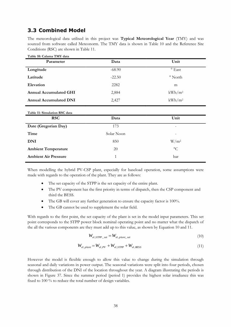
38
3.3 Combined Model
The meteorological data utilised in this project was Typical Meteorological Year (TMY) and was
sourced from software called Meteonorm. The TMY data is shown in Table 10 and the Reference Site
Conditions (RSC) are shown in Table 11.
Table 10: Calama TMY data
Parameter Data Unit
Longitude -68.90 ° East
Latitude -22.50 ° North
Elevation 2282 m
Annual Accumulated GHI 2,884 kWh/m2
Annual Accumulated DNI 2,427 kWh/m2
Table 11: Simulation RSC data
RSC Data Unit
Date (Gregorian Day) 173 -
Time Solar Noon -
DNI 850 W/m2
Ambient Temperature 20 °C
Ambient Air Pressure 1 bar
When modelling the hybrid PV-CSP plant, especially for baseload operation, some assumptions were
made with regards to the operation of the plant. They are as follows:
The set capacity of the STPP is the set capacity of the entire plant.
The PV component has the first priority in terms of dispatch, then the CSP component and
third the BESS.
The GB will cover any further generation to ensure the capacity factor is 100%.
The GB cannot be used to supplement the solar field.
With regards to the first point, the set capacity of the plant is set in the model input parameters. This set
point corresponds to the STPP power block nominal operating point and no matter what the dispatch of
the all the various components are they must add up to this value, as shown by Equation 10 and 11.
setplantelsetSTPPel WW _,_, (10)
BESSelSTPPelPVelplantel WWWW ,,,, (11)
However the model is flexible enough to allow this value to change during the simulation through
seasonal and daily variations in power output. The seasonal variations were split into four periods, chosen
through distribution of the DNI of the location throughout the year. A diagram illustrating the periods is
shown in Figure 37. Since the summer period (period 1) provides the highest solar irradiance this was
fixed to 100 % to reduce the total number of design variables.

39
Figure 37: Annual DNI at Calama
The daily variations were split into three periods throughout the day and were chosen based on the
standard daily electricity generation curves of the SING, the northern electricity system in Chile. These
periods are illustrated by the Figure 38. Since the peak hours are in period three, this period was fixed to
maximum load in the simulations to reduce the total number of decision variables.
Figure 38: Daily SING generation curve [115]

40
3.3.1 Dispatch Strategy
The plant can operate with two separate dispatch modes:
1. Prioritise the PV/BESS
2. Minimise the turbine shutdown
Using dispatch strategy 1, the PV and the BESS is prioritised over the CSP. That is to say that if the PV
capacity is large enough to cover the load, it does and the STPP is shutdown. The same can be said for the
BESS, i.e. if the BESS discharge capacity is large enough to cover the load, it does and the STPP is
shutdown for the period that the battery discharges. However, the STPP must be shutdown only if it
remains offline for a sufficient amount of time. As was mentioned previously, in Chapter 2.4.1, a turbine
hot start can take as long as 1-2 hours. Therefore it does not make sense to shutdown the plant for less
than 2 hours.
Implementing dispatch strategy 2, the minimisation of turbine shutdowns is the priority when the
different components are dispatched. This affects the dispatch of the PV, the BESS and the boiler in
certain aspects. The steam turbine has a minimum load, set at approximately 30% its gross power output,
and the dispatch ensures that the CSP power output never drops below this value [78]. The reasons for
this are because part load operation significantly reduces the efficiency of the turbine and also because
operating at such a load can cause failure in the turbine [116]. Due to this, if the electricity generated by
the PV is significant enough so that CSP power output approaches this value, additional PV electricity is
curtailed or used to charge the BESS. Furthermore the maximum discharge capacity of the BESS is set
that doesn’t exceed the same point. Examples of daily operation of these dispatch strategies can be found
in Figure 39.
Figure 39: Daily operation with dispatch strategy 1 and 2
Figure 40 shows a flow chart illustrating the flow logic of the plants dispatch, where TS is the timestep,
HTL is the hot tank level as a percentage, SOCBESS is the stage of charge of the BESS, DOD is the depth
of discharge of the BESS. WSET, WCSP, WPV and WBESS are the plant power output set point and the power
outputs of the respective plant components. Wmin_turb is the net minimum allowable power output from
the turbine. The flow chart, for the most part, represents dispatch strategy 2 while the grey boxes
represent the additional logic operations for dispatch strategy 1.

41
It can be seen by the figure that if the TES hot tank level is greater than 5%, the STPP will operate.
Thereafter, depending on the dispatch strategy and the capacity of the PV plant, the load is covered either
by the STPP alone, the PV plant alone or a combination of the STPP and the PV plant. If the TES hot
tank level is below 5%, the STPP shuts down. Thereafter, if there happens to be usable capacity in the
BESS and depending on the dispatch strategy and the capacity of the PV plant, the load is either covered
by the BESS entirely, by a combination of the BESS and the PV plant, a combination of the BESS and the
GB or the GB entirely. If the BESS is fully discharged then the load is covered by either a combination of
the GB and the PV plant or entirely by the GB.
Figure 40: Dispatch strategy flow chart
3.3.2 Operating Modes
The performance of the hybrid PV-CSP plant is dependent on the operating strategy implemented. For
the proposed plant, an operating strategy consisting of six different operating modes (OM) has been
defined. These OMs are visually represented by Figure 41 and described in detail in Table 12. It can be
seen in the table and figure that OM1a and OM3a are variations of OM1 and OM3 which have dispatch
strategy 1 implemented and have a PV capacity or BESS discharge capacity to cover the entire load. In the
figure the thick lines represent the molten salts HTF cycle and the thin lines represent the water/steam
cycle and the PV plant circuit. The black lines signify that there is energy stored or energy flowing in those
particular components or cycles. The grey lines signify that the plant components/cycle are currently idle
or shutdown.

42
Figure 41: Operating modes of hybrid PV-CSP plant

43
Table 12: Operating modes of hybrid PV-CSP plant
OM 1: PV is online , STPP is online, energy from solar field
The TES is charged by the energy from the solar field.
The TES discharges at a flow rate depending on how much power is needed to supplement the PV.
The PV power is constrained so that the turbine power never drops under its minimum value.
If there surplus energy from the PV it is used to charge the BESS.
If the BESS is fully charged the surplus energy is curtailed.
OM 1a: OM 1, PV power can cover full load, dispatch strategy 1
If PV generation is sufficient to cover the load, it does.
STPP is shutdown and energy coming from the solar field charges the TES.
If TES is fully charged then energy coming from the solar field is spilled.
If there surplus energy from the PV it is used to charge the BESS.
If the BESS is fully charged the surplus energy is curtailed.
OM 2: PV offline , STPP is online, no energy from solar field but enough in TES
The TES has enough energy to supply the demand.
During this mode no flow enters the TES hot tank, which simply discharges at the nominal flow rate.
No power coming from the PV.
BESS is idle.
OM 3: PV offline , STPP is online, no energy from solar field, not enough in TES, BESS charged
The TES does not have enough energy to supply the required demand and is idle.
The BESS is discharged but is constrained so that the turbine power never drops below its minimum
value.
The GB provides energy to the power block to supplement the BESS.
OM 3a: OM 3, BESS power can cover full load, dispatch strategy 1
If BESS capacity is sufficient to cover the load, it does.
STPP is shutdown.
OM 4: PV offline , STPP is online, no energy from solar field, not enough in TES, BESS discharged
The TES does not have enough energy to supply the required demand and is idle.
The GB provides the energy to the power block to cover the entire load.

44
3.3.3 Dynamic Model
The dynamic model is built using the TRNSYS software. The coupling of all the technologies occurs there
and therefore it is used to perform the transient simulations of the complete power plant. The dynamic
model requires the following as an input, which comes from the MATLAB steady state design and input
data. Using these inputs the dynamic model simulates plant operation for a year of operation gives the
relevant output necessary for the techno-economic calculations.
Weather data
Plant design point and component sizing
PV AC power output
The Wset taking into account the seasonal and daily variations in power output
Solar field efficiency
3.3.3.1 Control System
The most important coupling point is between the PV plant and the STPP, as the STPP output will need
to be regulated in accordance to the PV output at any given time. This is accomplished through a
proportional integral derivative (PID) controller. In this case the controlled variable is the net power
output from the STPP and is controlled by varying the mass flows rate of the HTF from the hot tank. The
tuning of the controller is carried out manually until the desired output is achieved [117]. The following
values for the PID controller at different simulation timesteps were developed.
Table 13: PID controller parameters
Timestep 10 minutes 30 minutes 1 hour
Gain Constant 5500 4000 4000
Integral Time 0.11 0.11 0.20
Derivative Time 0.1 0.05 0.01
These controller parameters are utilised to adjust the controller response time. With an increase time
response can lead to increased oscillations and decreased oscillations can lead to a slow response time. A
satisfactory trade-off between these two factors must be decided upon depending on the application of
controller. Figure 42 illustrates the operation of the PID controller and the trade-off between the
minimisation of the response time and oscillations. For a timestep of 10 minutes the simulation accuracy
was good but the computational time was too long. For a timestep of 1 hour, the computational time was
short but the accuracy suffered. For the final simulations, a timestep of 30 minutes was chosen because it
gave the satisfactory simulation accuracy with a reasonable computational time.

45
Figure 42: PID controller tuning [118]
3.3.4 Techno-economic Calculations
After the steady state and dynamic simulations are complete, the results are used in the techno-economic
calculations to calculate the performance indicators. This section describes the performance indicators and
the equations and cost functions used in these calculations
3.3.4.1 Levelised Cost of Electricity
The main performance indicator chosen to measure the economic performance of this plant is the
levelised cost of electricity (LCOE). The LCOE is a measure of cost per unit energy produced over the
course of the plant life. It is a very convenient indicator because it allows the comparison between
different energy technologies even if the scales of operation and level of investments are different [119]. It
is also particularly relevant for power plants operating baseload as they would need to produce a
maximum amount of electricity at a lowest cost possible. The LCOE of the proposed plant is the
combination of all the cash flows divided by the combined electricity production of all the plant
components during its lifetime and is shown by Equation 12.
N
n n
n
PVBESSCSP
N
n n
BESSBESS
N
n
N
n n
PVPVn
CSPCSP
DR
SDRFYEFYEFYE
DR
OPEXCAPEX
DR
OPEXCAPEX
DR
OPEXCAPEX
LCOE
1
11 1
1
1
111
(12)
where CAPEXCSP, CAPEXPV and CAPEXBESS stand for the investment cost of the CSP plant, PV plant
and the BESS respectively. The yearly fixed operational and maintenance costs of the components are
given by OPEXCSP, OPEXPV and OPEXBESS respectively. The CAPEX and OPEX of the boiler are
included in the cost of the CSP plant as it is implemented within the STPP. N and n correspond to the
total and current year of the project respectively [120]. This summation is accomplished using a discount
rate (DR). In this case we are assuming that the investment comes from a bank loan, and so the DR is set
to the interest rate; which can the real or the nominal interest rate. In order to adjust for years of
inflation, the real discount rate is preferred for long-term studies [119]. FYECSP, FYEPV and FYEBESS
correspond to the first year electrical output of each plant component. These values are also summed for
the lifetime of the plant using the DR. PV performance degrades with time and so a degradation factor
(SDR) is taken into account [120] [121]. The SDR is considered to be 0.79% of the nominal electricity
production as suggested in works by Jordan et al, 2012 [122]. As was mentioned in Chapter 3.2.3, the

46
battery performance also degrades with time. This form of degradation is characterised in terms of cycles
and has been taken into account within the FYEBESS prior to the LCOE calculation. The CSP plant also
has a degradation factor but the value is so small that it is considered negligible (0.2%) in this study [123].
A scenario is also examined in this case where the tax regulations of Chile allow for some certain tax
benefits, which can include tax deductions and an accelerated depreciation [124]. For this case, the tax
included in the CAPEX of all the components is returned and the value after tax of the fixed OPEX costs
is considered as a tax deduction. Furthermore, a depreciation tax shield can also be incorporated by
multiplying the current depreciation by the tax rate [124]. A double accelerated approach to calculate
depreciation was used in this thesis work. Accelerated depreciation currently exists in Chilean tax law but
the time scale is not known [125]. Therefore it is assumed that the valid time scale for the depreciation tax
benefits is 10 years. These modifications to the LCOE equations are shown in Equation 13 and 14.
YieldyElectricitLifetime
FlowsCashFlowsCashFlowsCashLCOE
BESSPVcsp
(13)
N
n
Nd
n nnTR
DR
DEPTR
DR
OPEXTAXCAPEXFlowsCash
1 11
11
(14)
3.3.4.2 Plant Cost Functions
The following section details the procedure used to calculate the CAPEX and OPEX of all plant
components including reference values. The cost functions are mainly based in typical reliability cost-
scaling equations, such as Equation 15, where the cost of component (Cn) is calculated using a reference
cost (Cref,n) multiplied by the ratio between the component size and its reference size. The scaling
coefficient varies for each cost component and is based on literature [126] [127]. Some cost functions,
mainly related to the PV and BESS, are based on specific costs ($/W) and so this cost-scaling approach
doesn’t apply. For the case of PV modules and inverters it was possible to obtain real quotations from
technology suppliers in the locations of interest.
yn
nref
nnrefn
X
XCC
,
, (15)
3.3.4.2.1 STPP
On the CSP side, the CAPEX is split into direct and indirect components, as shown by Equation 16. The
direct CAPEX consists of the investment associated to the power block (CPB) solar field (CSF), storage
(CTES), tower receiver (CTower), GB (CGB), (if necessary), balance of plant (CBOP), land adaptation and
contingency costs (CSite and Ccont). The indirect CAPEX covers all the remaining costs for the upfront
investment that are not directly related to the installation and purchase of equipment. These costs include
the tax costs (CTAX), the purchase of land (CLand) and the engineering, procurement and construction
(CEPC). The equations for the direct and indirect CAPEX are shown by Equations 17 and 18.
CSPdirectCSPdirectCSP CCCAPEX ,, (16)
ContSiteBOPGBTowerTESSFPBCSPdirect CCCCCCCCC , (17)

47
TAXLandEPCCSPindirect CCCC , (18)
The CSP OPEX is shown by Equation 19. The costs of utility (CUtility) represent services like water and
electricity, among others necessary to run the plant. The services costs (CServ) account for additional
services not related to the plant operation. The miscellaneous costs (Cmisc) account for the operation
overheads. The labour costs (CLabor) are related to the personnel necessary to operate the plant.
Additionally if the boiler backup is included, the fuel costs (CFuel) are added the overall OPEX. The costs
functions and technical/cost references used in the analysis can be found in Appendix K, L, M and O.
FuelInsuranceMiscUtilityServLaborCSP CCCCCCOPEX (19)
3.3.4.2.2 PV Plant
The PV component is also split into direct and indirect components. The direct components include the
cost of the PV modules (CPV), the cost of the inverters (CInv), the cost of the DC-DC converters (CConv),
the balance of system costs (CBOS), contingency costs (Ccont) and the cost of the tracking system (CTracking).
The indirect costs include the engineering costs (CE&D), land costs (CLand) and tax (CTAX). Equations 20, 21
and 22 represent the PV CAPEX equations.
PVindirectPVdirectPV CCCAPEX ,, (20)
contTrackingBOSConvInvPVPVdirect CCCCCCC , (21)
TAXLandDEPVindirect CCCC &, (22)
The OPEX equations are shown in Equation 23. In this case, the utility costs are included in the labour
costs (CLabor,PV). It is also includes PV panel cleaning and inverter maintenance. CInsurance,PV details the
insurance costs of the plant.
PVInsurancePVLaborPV CCOPEX ,, (23)
3.3.4.2.3 BESS
The economic analysis of the BESS is based on works by EPRI, 2013 [45]. As was with the CSP and PV
components, the BESS CAPEX structure is split into direct and indirect costs. In this case the direct
CAPEX costs are related to the battery modules (Cbat), the power conditioning system (PCS) (CPCS), the
balance of plant (CBOP) and the installation costs (Cinstal). The balance of plant costs are considered to be
the civil works costs only [128] [45]. If the BESS is coupled on the DC side then the cost of the PCS is
not considered as it is integrated with the PV PCS [45]. The indirect costs are characterised by the
engineering and contractor costs (CE&C), the softs costs (CSoft) which represent the process and project
contingency costs and the tax costs (CTAX). Equations 24, 25 and 26 represent the CAPEX calculations.
BESSindirectBESSdirectBESS CCCAPEX ,, (24)
instalBOPPCSbatBESSdirect CCCCC , (25)
TAXSoftCEBESSindirect CCCC &, (26)
The OPEX of the BESS consists of three main variables CFixed, CVariable and CReplacement. CFixed accounts for
the fixed O&M costs which mainly consist of maintenance of the PCS. CVariable represents the variable
costs associated of the discharge of the system; these costs include the cost of electrical losses used to

48
maintain the PCS and the battery during hot standby intervals [45] [129]. CReplacement represents the costs
associated with the replacement of the battery modules after their life has ended. The OPEX equation is
shown by Equation 27.
placementVariableFixedBESS CCCOPEX Re (27)
3.4 Model Verification
In order to verify that the model operates to a reasonable standard, the nominal design point and dynamic
performance of the model is compared to existing power plant configurations. The STPP and PV plant
are verified separately and the combined PV-CSP plant is also verified. Verification of the BESS model
could not be performed as real case data could not be acquired for comparison.
3.4.1 STPP Model
Table 14 and Table 15 show the plant design parameters and the dynamic performance of the CSP plant
model in comparison to the Redstone CSP power plant. The SM among various other parameters were
not known and therefore needed to be assumed. As can be seen by the tables, the CSP model shows good
agreement with the Redstone CSP plant in terms of both economic and technical aspects.
Table 14: STPP model design parameters
Parameter Redstone
Unit Reference CSP Model Reference
Capacity 100 100 MWel [86]
Storage Size 12 12 h [86]
Cooling Method Dry Dry - [86]
TES Medium Molten Salts Molten Salts - [86]
Storage Type Two-tank Direct Two-tank Direct - [86]
Table 15: STPP dynamic performance
Performance
Indicator
Redstone Unit Reference
CSP Model Reference
Net Electricity
Yield 498 480 GWh/yr [76]
LCOE/PPA 0.114 0.124 $/kWh [76]
Investment 519 500 $mill [130]
3.4.2 PV Plant Model
Table 16 and Table 17 show the design parameters and dynamic performance of the PV plant model in
comparison to real PV plants for the purpose of model verification. The PV plants chosen for the
comparative analysis are the Jasper and Lesedi PV plants currently operational in South Africa [89]. The
tilt angle of the PV modules was not known but it was assumed to be 28.43°, the latitude of the location.
The PV model shows good agreement with the real cases in terms of annual electrical yield and
investment costs. However there is some discrepancy regarding the number of PV modules, especially in
the case of Jasper.

49
Table 16: PV plant design parameters
Parameter Jasper Lesedi
Unit Reference PV Model Reference PV Model Reference
Capacity 75 75 64 64 MWac [89]
Tracking Fixed-tilt Fixed-tilt Fixed-tilt Fixed-tilt - [131]
Tilt angle 28.43 Unknown 28.43 Unknown °
PV module
Yingli
YL295P-
35b_295Wp
Yingli
YL295P-
35b_295Wp
Hanwha
SolarOne
SF270
Hanwha
SolarOne - [131] [132]
Inverter Ingecon Sun
PowerMax
Ingecon Sun
PowerMax
Ingecon Sun
PowerMax Unknown - [133] [132]
Table 17: PV plant dynamic performance
Performance
Indicator
Jasper Lesedi Unit Reference
PV Model Reference PV Model Reference
PV modules 287850 325480 263872 277632 - [133] [132]
Inverters 75 78 64 64 - [133]
Net Electricity
Yield 189 180 159 150 GWh/yr [89]
Investment 226 230 190 190 $mill [133] [132]
3.4.3 PV-CSP Model
Table 18 show the dynamic performance of the hybrid PV-CSP plant model in comparison to Copiapó
and Atacama 1. The design parameters of the two plants can be found in a previous chapter, Chapter
2.4.3. The solar multiple of the CSP plant components, along with other plant parameters, were unknown
and needed to be assumed. The analysis shows good agreement with regards to the net electrical yield and
the investment costs. There is some discrepancy between the LCOE and PPA of Atacama 1. The reason
for this is that the PPA issued is for the first year of operation while the LCOE takes into account the
entire life of the plant. The LCOE changes every year of operation due to the discount rate employed.
Table 18: PV-CSP plant dynamic performance
Performance
Indicator
Copiapó Atacama 1 Unit Reference
Model Reference Model Reference
Heliostats 11,816 13,750 15,808 10,600 - [81] [86]
PV Modules 313,348 Unknown 416,423 431,480 - [81] [87]
Capacity
Factor 99 Baseload 99 Baseload % [81] [87]
Net Electricity
Yield 949 850+ 958 950 GWh/yr [81] [134]
Investment 1,019 1,000 1,087 1,300 $mill [83] [88]
LCOE 139.47 Unknown 125.61 114.92 $/kWh [134]

50
3.5 Multi-Objective Optimisation
In order to carry out an effective analysis into the feasibility of the proposed power plant, optimisation
studies were performed. Optimisation is a method of determining the optimal plant configuration for a
given range of design variables, for a given design objective. Multi-objective optimisation is the
determination of a range of optimal plant configurations for multiple and often conflicting design
objectives. By solving these multi-objective problems, the solution gives rise to a trade-off curve, known
as a pareto curve [135]. An example of a pareto curve is illustrated by Figure 43.
The optimisation is based on an evolutionary algorithm that uses a population based approach. In this way
more than one solution participates in a solution iteration which in turn evolves to create new population.
The main advantages of these algorithms are that they are flexible, simple to implement and can be used
for a wide spread of applications. The evolutionary process is characterised by four main steps: selection,
cross-over, mutation and elite-preservation. The process stops when the user requirements are met or
when the maximum amount of iterations has been reached. The initial population was set with regards to
work by Leyland, 2002 [136]. The initial population evolves to the solution of the optimization through
means of two operations; where new individuals are created and individuals are removed. These
operations are known as cross-over and mutation [135] [136]. The cross-over operation selects two or
more individual solutions (parents) and creates a new individual (child) by exchanging information
amongst the parents. Mutation involves altering an individual slightly, much like the natural mutation
found in nature. In order to increase the likelihood of a “good” child, the parents can be selected from
better parts of the population, much like breeding. Lastly, the elite-preservation operator combines the
newly created population with the old one and keeps the better solutions for the next iterations. This step
is necessary to ensure a convergence to the optimal trade-offs curves [135].
Figure 43: Pareto curve illustration [136]

51
3.5.1 Design Variables and Objectives
Table 19 shows the design variables chosen for the multi-objective optimisations. Two cases were chosen
for comparison for the hybrid model. The design objectives of these cases are shown in Table 20. For
case 1, the minimisation of plant CAPEX was chosen as the second design objective. The reason for this
is because it is an important factor when it comes to investment in projects that contain relatively new
technologies, such as the proposed hybrid plant. For case 2, the minimisation of plant CO2 emissions was
chosen as the second design objective. This is an interesting case from a sustainability point of view but
also because of the plant location, i.e. Chile is focused on the promotion of renewable energy, not fossil
fuels. Two fixed capacity case optimisations were also performed. The design variables and objectives are
exactly the same, with the only difference being that the CSP capacity is removed as a variable.
Table 19: Multi-objective optimisation design variables
Variable Range Unit
STPP
CSP Net Power 50 -250 MW
Solar Multiple 1 - 4 -
Storage Size 10 - 22 h
Heliostat Area 46 - 160 m2
Receiver Diameter 8 - 22 m
Tower Height 145 - 280 m
Seasonal Output Variance 80 - 100 %
Daily Output Variance 80 - 100 %
PV Plant
PV Net Power 0 - 250 MWac
Tilt Angle 20 - 45 °
Tracking Mode 2 - 4 -
BESS
Battery Capacity 0 - 250 MWh
Battery Technology 1 - 4 -
Battery Dispatch Mode 1 - 2 -
Battery Coupling DC & AC -
Table 20: Multi-objective optimisation design objectives
Case Performance Indicator Objective Unit
Case 1 LCOE Minimise $/MWh
CAPEX Minimise $mill
Case 2 LCOE Minimise $/MWh
CO2 Emissions Minimise kg

52
4 Results
The section details the results of the multi-objective optimisation study of the complete PV-CSP hybrid
plant for the two aforementioned cases. The section also details the results of the fixed capacity cases.
They were performed to get a full understanding of how the contribution of different plant components
varies for a fixed plant capacity. Furthermore additional plant configurations were chosen and compared
against each other and completing technologies; CSP alone and PV-diesel genset hybrid.
4.1 Case 1: Minimise LCOE and CAPEX
The following figures show the optimal pareto curve in terms of the LCOE and CAPEX and a third
variable. The curve is constructed by a large quantity of dots, each of which represent a particular plant
configuration. The LCOE and CAPEX values are those which take into account the previously described
tax incentives. Figure 44 shows the optimal configurations in terms of the STPP/plant capacity, the PV
capacity and the BESS capacity. It should be noted that the valid pareto-front exists at the bottom section
of the curve until it reaches the bend. At this point the plant capacity has converged to a minimum. To
achieve lower LCOE values, the STPP/plant capacity increases while the PV capacity and the BESS
capacity have both converged to zero throughout. Therefore the CAPEX is entirely dependent on the
capacity of the STPP.
(a) (b)
(c)
Figure 44(a): STPP/plant capacity; (b): PV capacity; (c): BESS capacity

53
Figure 45 describes the percentage contribution of each plant component to the total annual electricity
yield. Throughout the valid pareto-front, the majority contribution comes from the STPP with the GB
supplementing the rest. Beyond this section, for very low CAPEX values, the contributions made by the
GB become more significant, contributing to 40-50% of the total generation. In this case the GB is
replacing the power lost from a decreasing solar field. Since the BESS and PV capacity converged to zero,
both make no contribution throughout the pareto-front. At this point it can be seen that the GB is
preferred over PV. Due to the design objectives applied, this is purely from an economical aspect.
(a) (b)
Figure 45(a): Ratio of annual power generation from STPP; (b): Ratio of annual power generation from GB
Figure 46 describes the SM and TES capacity for the range of optimal solutions. The SM converges to
approximately 2.5 through the pareto-front. The TES capacity shows an increasing trend with a decreasing
LCOE. The segregation that forms at the top of the curve, beyond the pareto-front, is due a decreasing
SM. The optimisation alters the SM to a degree of one decimal place, the result of which can be seen in
region of the curve. Figure 47 describes the utilisation of the GB in greater detail through the annual NG
consumption and OPEX, the latter of which can be seen to be almost entirely dependent on the former.
The GB is utilised the least at the end of the pareto-front where the CAPEX is the lowest.
(a) (b)
Figure 46(a): Solar multiple; (b): TES capacity

54
(a) (b)
Figure 47(a): Annual consumption of NG; (b): Annual OPEX
Figure 48 describe the variations in load in the spring and winter seasons. In the spring period the load
converges to almost 100%. A similar trend can be seen in the autumn period. This is the opposite for the
winter period however. Since this is the worst period in terms of DNI, the GB must operate for more
time. The curve tends to approximately 85% to reduce the use of the GB as this increases the annual
OPEX significantly. Beyond the valid pareto-front, the load values become more sporadic. The daily
period curves show the same convergence as the spring period.
(a) (b)
Figure 48(a): Output variations in spring period; (b): Output variations in winter period

55
4.1.1 Single Capacity Case
The following figures show the pareto optimal curve for case 1 for a fixed capacity. The capacity chosen
was 200 MW, as it was thought to be interesting to see how the pareto curve forms around such a high
capacity plant. Figure 49 describes the capacities of the PV component and the BESS component. As was
with the first study, both technologies have converged to a minimum.
(a) (b)
Figure 49(a): PV capacity; (b): BESS capacity
As was with the previous case, the SM converges to approximately 2.5 for lower LCOE values and
decreases for lower CAPEX values. In this case the segregation in the curve is more prominent due to the
capacity being fixed. Figure 50 shows the contribution made by the plant components to the total annual
electricity yield. The STPP covers the majority of the annual yield for lower LCOE values, with the GB
supplementing it with approximately 20% coverage. As the SM decreases, the power from the solar field
decreases and is replaced with energy from the GB. Since the capacities of the PV and BESS components
converged to zero, their contributions were both zero.
(a) (b)
Figure 50(a): Ratio of annual power generation from STPP; (b): Ratio of annual power generation from GB

56
4.2 Case 2: Minimise CO2 emissions and LCOE
The following pareto curve represents the design objectives, LCOE and CO2 emissions, in terms of a
third variable. Figure 51 shows the optimal pareto-front in terms of the individual plant components.
Furthermore, Figure 51(d) shows the ratio of the PV capacity to the STPP capacity. It should be noted
that the valid pareto-front exists from the upper left section of the curve until the bend. At this point the
plant capacity has converged to its minimum value, which does so to minimise the emissions. To achieve
lower LCOE values, the STPP/plant capacity increases resulting in increased CO2 emissions. In this
region, the SM and TES capacity converge to approximately 2.4 and 22 hours respectively. Even though
the CAPEX would naturally increase, the increased annual electrical yield results in a reduction in LCOE.
The PV capacity converges to very small capacities throughout the pareto-front but becomes more
significant beyond it in order to achieve low CO2 emissions; so much so that its capacity becomes larger
than the overall plant capacity. At this point an increased amount of PV power is spilled. This spilled
power accounts for both DC power curtailment due to the inverter and AC power curtailment due to
either the BESS being fully charged or that no BESS exists. In this region BESS capacity also increases
rapidly but the LCOE values are very high.
(a) (b)
(c) (d)
Figure 51(a): STPP/plant capacity; (b): PV capacity; (c): BESS capacity; (d): Ratio of PV capacity to CSP

57
(a) (b)
(c) (d)
Figure 52(a): Ratio of annual power generation from STPP; (b): Ratio of annual power generation from PV; (c): Ratio of annual power generation from BESS; (d): Ratio of annual power generation from GB
Figure 52 describes the contribution made by each plant component to the total annual electricity
generation. In the pareto-front, the contribution is made mainly by the STPP and supplemented by the
GB, whose contribution is limited to below 10%. At lower emission values, beyond the pareto-front, this
contribution is split between the STPP and the PV, the latter of which achieves up to 50%, with little to
nothing generated by the BESS or the GB. Figure 53 describes the variations in load for the spring and
winter period. The spring load increases from approximately 94%, as the LCOE decreases, and eventually
converges to a maximum value. The winter load converged to a minimum throughout the valid
pareto-front in order to mitigate the use of the GB. As was with the previous case, this is due to the poor
DNI values of the winter period in comparison to the other seasonal periods. The autumn and second
daily load values converged to approximately 88% and 94% respectively while the first daily load period
converged to a maximum.

58
(a) (b)
Figure 53(a): Output variations in Spring period; (b): Output variations in Winter period;
Figure 54 describes the variations in CAPEX throughout the pareto front. The region where the CAPEX
is at its lowest value is when the plant capacity is at its lowest and increases with an increase in capacity. As
the plant emissions are reduced further, the introduction of PV capacity also begins to increase the
CAPEX.
Figure 54: CAPEX
4.2.1 Single Capacity Case
A fixed capacity case was also performed for a capacity of 200 MW, the value of which was chosen the
sake of consistency. Figure 55 describes the capacities of the PV and BESS components, as well as the
ratio of PV capacity to CSP, throughout the pareto-front configurations. For low LCOE values the PV
capacity converges to zero but becomes more significant for low emissions values. In this region the PV
to CSP capacity ratio reaches approximately 1-1.2. A similar trend can be seen in the BESS capacity.
Furthermore, the SM converged to a value between 2 and 2.5 and the TES capacity converged to 22 hours
through the pareto-front.

59
(a) (b)
(c)
Figure 55(a): PV capacity; (b): BESS capacity; (c): Ratio of PV capacity to CSP capacity
Figure 56 shows the contribution made by the plant components to the total annual electricity yield. As
was with the previous case 2 analysis, the CSP dominates for low LCOE values with a maximum of 10%
covered by the GB. The contribution made by the PV increases to 30-40% for low emissions values.
While there is a contribution made by BESS, it is so small that it does not register in terms of yearly
operation and therefore is not shown in the figure. Figure 57 describes the variation of the CAPEX
through the pareto-front. In this case the CAPEX converges to a minimum of approximately
$1 billion for lower values of LCOE. This is because the capacity is fixed and the SM is relatively stable in
this region. For lower emissions values, the increase of the PV capacity results in a significant increase in
CAPEX to approximately $2 billion and more.

60
(a) (b)
(c)
Figure 56(a): Ratio of annual power generation from STPP; (b): Ratio of annual power generation from PV; (c): Ratio of annual power generation from GB
Figure 57: CAPEX

61
4.3 Dynamic Performance
Plant configurations were chosen from the pareto-fronts of all the above cases to examine their plant
configurations and their dynamic performance in greater detail. In Figure 58, Point A1, B1, A2 and B2
describes where these configurations lie in their respective pareto curves. Point A1 was chosen due to its
location on the pareto-front and because its capacity is standard in large CSP plants, i.e. the capacity of
Copiapó, Atacama 1 and Atacama 2. Point A2 was chosen with the same plant capacity of point A1 and
the lowest possible LCOE, so that a comparison could be made. Point B1, from the fixed capacity case of
case 1, was chosen due to its location at the bottom of the pareto curve. Point B2, from the fixed capacity
case of case 2, was chosen due its location of optimal trade-off. The key design parameters and
performance indicators for these plant configurations A1 and A2 are shown below in Table 21.
(a) (b)
(c) (d)
Figure 58(a): Case 1 Point A1 configuration; (b): Case 2 Point A2 configuration; (c): Case 1 Point B1 configuration; (d): Case 2 Point B2 configuration

62
Table 21: Point A design parameters and performance indicators
Parameter A1 A2 Unit
CSP Capacity 110 110 MW
SM 2.5 2.5 -
Storage 21 22 h
PV Capacity 0 1 MW
Tracking - Single-Axis -
Tilt - 22 °
BESS Capacity 0 6.12 MWh
Technology - Li-NMC -
Coupling - AC -
Dispatch Strategy - 2 -
Seasonal Power Output 0.99/0.81/0.99 0.86/0.84/0.93 Aut/Win/Spr
Daily Power Output 0.99/0.99 0.98/0.98 0-9h/10-20h
NG Consumed 26086 19834 m3/year
CO2 Emissions 50.09 38.08 MTon/year
Annual Electrical Yield 919.54 886.00 GWh/year
CAPEX 793.59 808.86 mil$
OPEX 25.57 21.76 mil$/year
LCOE 110.35 111.94 $/MWh
Capacity Factor 99.24 99.44 %
Figure 59 and Figure 60 describe the operation of plant configuration A1 and A2 over a week. The week
presents good variation in terms of solar resource quality, as can be seen by the power coming from the
solar field on day 1 and day 3. In this way, an in depth examination of the entire plant operation can be
carried out. Plant A1 describes a plant of standard CSP capacity with no PV or BESS. Instead it uses the
GB as backup when needed. With a large solar field and storage, which discharges to approximately 50%
on good solar days, it can cover the majority of its annual generation with the STPP alone. Therefore this
suggests that it more economical, from a combined LCOE and CAPEX point of view, to implement a
large solar field and TES system while sparingly utilising the GB instead of implementing either PV or
BESS. Plant A2 describes a plant of similar configuration but with an increase TES size and the
introduction of a small amount of PV. Both of these variations are implemented to limit the use of the
GB. This can be seen by the NG consumed, the CO2 emissions and OPEX of the two plant
configurations in Table 21. Furthermore the seasonal and daily output loads converge to smaller values to
mitigate the use of the GB further. All in all, these alterations result in an increased CAPEX and a
decreased annual electrical yield resulting in an overall larger LCOE. Finally it can be noted that the
capacity factors of both plant configurations are almost 100% thereby ensuring that baseload operation
has been satisfied

63
Figure 59: Week operation of Plant A1
Figure 60: Week operation of Plant A2
A full breakdown of the specific CAPEX and OPEX values for each plant component of both plant
configurations can be seen in Figure 61. The plant CAPEX values of both configurations are dominated
by the STPP costs while the OPEX are dominated by the OPEX values from the GB. The contribution
of the GB to the OPEX of plant A1 is larger because it operates from more time during the year. In the
case of plant A2 the PV capacity is small enough that it does not really impact the overall cost breakdown.

64
Figure 61: CAPEX and OPEX breakdown of plant A1 and A2
The plant parameters and key performance indicators of plant configuration B1 and B2 are shown in
Table 22. In this case optimal plant configurations were extracted from the 200 MW fixed cases. Plant B1
has relatively large solar field and a large TES of 22 hours. This allows the STPP to cover the majority of
the annual production. This can be seen in Figure 62 where, on a normal day, the TES discharges to
approximately 50%. This reiterates the point made with plant A1 that implementing a large solar field and
TES with limited use of the GB is more economical, in terms of LCOE, than implementing PV and
BESS. Plant B2 incorporates an equally sized TES and slightly smaller solar field but with the addition of
PV and BESS capacity. The PV-CSP ratio is approximately 0.4 and even though dispatch strategy two is
implemented the PV curtailment, seen in Figure 63, is from the DC side. This combined with the fact the
BESS is coupled from the AC side means that this curtailed power is spilled and not used to charge the
BESS. Perhaps if the simulation ran for more iterations the BESS would have converged entirely to zero.
With these variations, plant B2 consumes only 30% the amount of NG consumed by plant B1. This also is
evident in the weekly operation of this plant in Figure 63. The seasonal and daily load percentages are also
reduced to mitigate the use of the GB, as was with plant A2. As a result the emissions, OPEX and annual
electrical yield are reduced while the CAPEX and LCOE are increased. It can also be noted that these
plant configurations have satisfied their baseload operation with very high capacity factors.

65
Table 22: Point B design parameters and performance indicators
Parameter B1 B2 Unit
CSP Capacity 200 200 MW
SM 2.2 2.0 -
Storage 22 22 h
PV Capacity 0 81 MW
Tracking - Dual-Axis -
Tilt - 34 °
BESS Capacity 0 9 MWh
Technology - Li-NMC -
Coupling - AC -
Dispatch Strategy 2 2 -
Seasonal Power Output 0.86/0.82/0.97 0.80/0.81/0.88 Aut/Win/Spr
Daily Power Output 0.84/0.86 0.80/0.80 0-9h/10-20h
NG Consumed 43814 12859 m3/year
CO2 Emissions 84.12 24.67 MTon/year
Annual Electrical Yield 1452.32 1343.95 GWh/year
CAPEX 1230.04 1410.90 mil$
OPEX 41.34 24.28 mil$/year
LCOE 109.55 121.51 $/MWh
Capacity Factor 99.02 99.37 %
Figure 62: Week operation of Plant B1

66
Figure 63: Week operation of Plant B2
A full breakdown of the CAPEX and OPEX values of each component for each plant configuration can
be seen in Figure 64. The CAPEX of plant B1 is dominated by the STPP once more while the OPEX is
dominated by the GB. Plant B2 has a different breakdown of costs with the PV contributing to a portion
of the CAPEX and OPEX, approximately 14% and 11% respectively. Even though the GB operates less
during the year than plant B1, it still contributed to a 33% share of the overall OPEX.
Figure 64: CAPEX and OPEX breakdown of plant B1 and B2

67
4.4 Comparison with Competing Technologies
In this section, two proposed plant configurations from case 1 and 2 are compared to a CSP alone
configuration and a PV-diesel genset hybrid both designed for baseload operation. The proposed
configurations are taken from the comparison are plant B1 and plant B2. These values were then matched
with the other technologies, in terms of plant capacity, and the key performance indicators and plant
parameters were compared. The results of this comparison can be found in Table 23.
Table 23: Comparison on different cases and plant configurations
Parameter B1 B2 CSP alone PV Genset Unit
CSP /Plant Capacity 200 200 200 200 MW
SM 2.2 2.0 4 - -
Storage 22 22 22 - h
PV Capacity 0 81 0 201 MW
Tracking - Dual-Axis - Dual-Axis -
Tilt - 34 - 30 °
BESS Capacity 0 9 0 0 MWh
Technology - Li-NMC - - -
Coupling - AC - - -
Dispatch Strategy 2 2 - - -
Seasonal Power
Output
0.86/0.82/
0.97
0.80/0.81/
0.88
0.75/0.74/
0.71
0.99/0.99/
0.98 Aut/Win/Spr
Daily Power Output 0.84/0.86 0.80/0.80 0.80/0.82 0.98/1.00 0-9h/10-20h
NG/Diesel
Consumed 34.18 10.00 0 336247.70 m3/year
CO2 Emissions 84.12 24.67 0 717.56 MTon/year
Annual Electrical
Yield 1452.32 1343.95 1251.98 1734.14 GWh/year
CAPEX 1230.04 1410.90 2224.12 575.64 mil$
OPEX 41.34 24.28 23.25 322.54 mil$/year
LCOE 109.55 121.51 188.49 226.40 $/MWh
Capacity Factor 99.02 99.37 97.10 100 %

68
As Table 23 shows, Case 1 performs the best in terms of LCOE and CAPEX with values of
$109 per MWh and $1230 million respectively. This is because these performance indicators were the set
design objectives of that study. With the regards to the LCOE, case 1 provides a 42% reduction in
comparison to CSP alone case and a 52% reduction in comparison to PV-diesel genset hybrid case. In
terms of CAPEX, case 1 provides a 45% reduction and a 113% increase in comparison to CSP alone and
the PV hybrid cases respectively. The CAPEX of the PV hybrid is low because of the technologies
involved. It also shows the highest OPEX, out of the CSP configurations, due to its use of the GB. Case 2
performed second best in terms of the same performance indicators. In order to reduce the CO2
emissions, the CAPEX and LCOE increased as the operation of boiler was replaced by a combination of
TES, PV and BESS. Furthermore the total annual electrical yield was reduced due to a reduction in the
seasonal and daily load tiers. However, case 2 still performed better than CSP alone or the PV-diesel
genset case. In terms of LCOE, case 2 provides a reduction of 35% and 46% in comparison to the CSP
alone and PV hybrid cases respectively. Furthermore, a vast decrease in CO2 emissions can be seen in
comparison to the PV hybrid case, of approximately 97%. However, an increase in emissions can be seen
when compared to CSP alone. The CSP alone case performed the best in terms of CO2 emissions but
shows the highest CAPEX value. This is due to the fact that the solar field is significantly larger than the
first two cases in order to achieve such a high capacity factor. The PV-diesel genset hybrid plant performs
the worst in terms of LCOE and OPEX with values of $227 per MWh and $323 million per year
respectively. This is because the diesel genset covers approximately 60% of the total annual generation. It
also performs the worst in terms of CO2 emissions by emitting more than eight times that of case 1. A
study conducted by Bloomberg, 2011, states that the levelised cost of electricity from a utility scale diesel
system is in the range of $346 - $560 per MWh [75]. The addition of cheap PV has reduced the LCOE but
it is still high in comparison to the other cases.

69
5 Discussion
This section details some final discussions on case 1 and 2, the single capacity cases and the final
comparisons of the chosen plant configurations against the each other and competing hybrid and
non-hybrid technologies. One of the main observations, especially from case 1, was that the optimisation
favoured the use of fossil fuel backup rather than PV to reach a cost-effective baseload configuration. The
overall reason for this is because, for the assumed cost functions, the chosen design objectives and the
method in which the backup boiler is implemented, it is the more economical alternative in terms of
CAPEX and LCOE. This was true even if the gas price in Chile is high in relation to other countries
implementing CSP technologies [58]. Because of the high NG price it was somewhat expected that PV
would be implemented to replace the high cost of the solar field at higher capacities. At high capacities the
solar field has to be very large to overcome attenuation losses [58]. However, rather using PV and
increasing the CAPEX, the optimisation chose to utilise the NG boiler backup which adds no additional
CAPEX but increases the OPEX of the plant. In case 2, similar tends were seen for the main study with
the variation of larger TES and the addition of a small amount of PV. However the implementation of PV
was more prominent for the fixed capacity case. As was mentioned, the PV capacity was increased in
order to mitigate the use of the GB to reduce the emissions from the GB. While the emissions are
reduced they come at a price of an increased CAPEX and decreased annual electrical yield. These facts
result in an increased LCOE which reiterates the aforementioned conclusion from case 1.
Another point relating to this conclusion is regarding the exact laws and legislation of the location. The
laws and legislation regarding the maximum amount of NG that can be consumed is not known nor the
method implementing NG backup boilers to CSP plants in Chile. This is due to the difficulty of obtaining
this type of information. The optimisation carried out in this thesis neglects any laws regarding these
matters and leaves the model to decide how the GB is utilised. As was previously discussed in Chapter 2,
the method of coupling the GB to the STPP is the most efficient for this application. However, perhaps if
there are specific laws and legislation present regarding boiler coupling, the outcome of this analysis could
be different. For example, in Spain depending on the condition of operation, a maximum of 12% - 15%
of the total energy generated of a CSP plant could be sourced from NG [2]. There was similar legislation
relating to the total amount of NG used for the backup of the SEGS plants in the United States. In this
case a maximum of 25% of the primary energy generated by the plant could be sourced from NG [2]. In
terms of the method of coupling, in Spain the GB could only be coupled to the HTF cycle and not the
steam cycle [137]. Another example is the Shams 1 plant in the United Arab Emirates which was required
to have a GB coupled to the HTF cycle by the utility [2].
The BESS was not favoured for either cases and the main reason for this is the current capital costs of the
equipment [18]. Furthermore, according to EPRI, 2012, Li-Ion batteries in BESSs have to be replaced
every 5 years and all other technologies have to be replaced every 7.5 years [128]. This short life of current
battery technologies is major technical limitation and one that is preventing its widespread use in large
scale storage systems. In case 1 the BESS was not favoured throughout the pareto-front due to the vast
increase in CAPEX implementing such as system would result in. However for case 2, where very low
CO2 emissions were achieved, BESS was implemented. Having said that, the addition of high capacity PV
and BESS have increased the CAPEX of the system to large values, thereby increasing the LCOE to
ranges of $250-300 per MWh. These values are far from competing with traditional fossil fuel plants in
Chile. For example, coal and combined-cycle gas turbine plants can generate electricity at a range of $73-
$155 per MWh and $68-$111 per MWh respectively [75]. PV plants can achieve costs of electricity as low
as $119 per MWh [6]. Large scale PV projects, such as Letsatsi in South Africa, have signed PPAs for
approximately $225 per MWh [138]. One project in particular, located in Dubai, signed an extremely low
PPA of $58.4 per MWh [139].

70
The dynamic performance of the A and B plant configurations offered a different look into the operation
of the hybrid plant. Firstly, key plant parameters and performance indicators were compared. Secondly, a
standard week of operation was displayed and finally the CAPEX and OPEX breakdown of each plant
was illustrated. It was shown that the main difference between the plant configurations was that, for the
case 2 configurations, the boiler operation was mitigated by using a larger solar field and a larger TES or a
smaller solar field with a significant PV capacity. BESS was also implemented but on such a small scale to
the overall plant capacity that it provided a negligible contribution. Furthermore the seasonal and daily
outputs were limited for the same reasoning. By doing so, the CAPEX increased and the annual electricity
yield was reduced, resulting in larger LCOEs.
The final comparison was one made with potential competing technologies, a STPP plant and a PV-diesel
genset hybrid plant, both designed for baseload operation. The results show that not only can the
proposed hybrid configuration B1 can compete with these technologies, but the more expensive B2 plant
can also too. These competing technologies were chosen from renewable technologies that could be
deployed in the region. As was mentioned previously, there is no opportunity for hydro power nearby in
the region [8]. A comparison can also be made regarding the optimisation results and the known PPAs
from the discussed hybrid PV-CSP plants in development, namely Copiapó, Atacama 1 and Atacama 2.
Atacama 1 and 2 have been awarded 950 GWhe per year at a PPA of $114.82 per MWh [134]. Copiapó
has yet to sign a PPA agreement but, based on current average electricity prices for the mines in the
Atacama region, it can assumed to be approximately $150 per MWh [140]. In reality the final PPA will
probably be lower this but for the sake of comparison this value will be utilised. The configurations of
these plants can be found in Chapter 2.4.3 in Table 5 and Table 6. Optimal plant configurations were
chosen based on the plant capacity of Copiapó and Atacama 1 & 2 and the comparisons between the
LCOE and PPA values can be seen in Table 24. As it shows, the LCOES values from the optimal case 1
and case 2 plants are lower than the assumed PPAs of Copiapó and the Atacama plants.
Table 24: Model LCOE and real case PPA comparison
Plant PPA Case 1 Case 2 Unit
Atacama 1 & 2 114.82 110.35 111.94 $/MWh
Copiapó 150.00 110.93 112.28 $/MWh

71
6 Conclusions
To conclude, a brief summary of the thesis work and results are outlined, focusing on the main outcomes.
Thereafter some final conclusions are made as well as recommendations on potential future work. The
objective of the work was to determine, for the Chilean market, whether or not a hybrid PV-CSP baseload
plant is more economically viable than a CSP plant or a hybrid PV-diesel genset plant. These objectives
were achieved through a number of steps. Firstly, an extensive literature review was conducted to gain a
full understanding of the technologies and the market. Secondly, the existing models in the DYESOPT
tool were familiarised with and improved on if needed. The main improvements that were made are with
regards to the computational time of the PV model. Thereafter the development of two further methods
of hybridisation, the BESS and the GB, were developed along with a complex plant operation strategy,
which included the two dispatch strategies. However, the analysis of the PV-CSP plant was done through
techno-economic means; taking into account technical, economic and environmental aspects. Therefore
not only were technical models created but also economic and emission calculations were required.
Thereafter the complete hybrid model was verified, along with its separate components, against real cases.
Multi-objective techno-economic optimisation studies were then performed to find the optimal trade-off
between two design objectives, for two separate cases.
The main outcomes of case 1 (minimisation of CAPEX and LCOE) were that, for the cost and technical
assumptions made, it is more economical favourable to implement a GB to supplement the STPP to
achieve baseload, than implementing PV or BESS. A fixed capacity case for the same design objectives
reiterated these conclusions. Case 2 (minimisation of CO2 emissions and LCOE), and the second fixed
capacity case, preferred the implementation of PV and reduced seasonal and daily loads in order to
mitigate the use of the GB. BESS was not favoured in either case due to the high costs related to the
technologies. Plant configurations from case 1 and 2 were chosen and compared against CSP alone and
hybrid PV-diesel. Case 1 showed a 42% and 45% reduction in LCOE and CAPEX, respectively, when
compared to CSP alone and a 52% reduction in LCOE when compared to the hybrid PV-diesel. Case 2
showed a 35% reduction in LCOE in comparison to CSP alone and a 46% and 97% reduction in LCOE
and CO2 emissions, respectively, when compared to hybrid PV-diesel. The results have shown that it is
more economically viable for a hybrid PV-CSP plant to operate baseload in comparison to CSP alone or
hybrid PV-diesel and therefore the hypothesis can be considered validated.
The concept of PV-CSP hybrid plants is one of great interest, especially in regions such as Chile and
South Africa where the weather climate and economic conditions are favourable for such projects. This is
evident with the development of PV-CSP hybrid plants, such as Copiapó and Redstone. Chile, in
particular, is attractive of high capacity solar plants due to the fact that there is a very good solar resource,
energy intensive mines which require baseload energy are located there, land is abundant and there are no
opportunities for nearby hydropower [8]. One other important point is that the country does not have or
produce domestic fossil fuels and has a strong community of environmentally conscious stakeholders [8].
This means that there is a great interest in developing clean energy plants that can operate with as little
fossil fuel backup as possible. Therefore, while one of the main outcomes of the thesis work is that it is
more economically favourable to implement NG backup rather than PV, the dynamics of the location
must be considered. Since the Chilean Government have been implementing strategies in the promotion
of a more diverse energy structure, one that consists of more generation from renewable sources, the
commissioning of high capacity factor solar plants that generate electricity almost entirely from solar
energy would be of greater interest than one that generates electricity at a lower cost, but that utilises a
significant amount of NG [93].

72
6.1 Future Work
Here is a list of some limitations of the project and some recommendations for future work.
The model does not consider any laws and regulations that may exist for the implementation of
fossil fuel backup to large renewable energy power plants. This could be researched and
implemented in the model in order to give a more accurate depiction of the plant configurations
that may be found in the location in the future.
Currently the model only takes into account the LCOE, CAPEX and OPEX as the only
economic performance indicators. It could be interesting to introduce a financial model that
could implement other indicators such internal rate of return or PPA calculation.
The model currently does not take into account the technical limitations of the steam turbine, in
terms of ramping up and down. Nor does it take into account frequency regulations issues
regarding grid integration. In reality these issues could be a strong point for the utilisation of
BESS and could be implemented in the model.
The control system, for the output of the STPP, implemented in the model has issues in terms of
stability, specifically during shutdown and start-up. The STPP has a slow response time when it is
started up, after the GB or the PV component have been operation. This results in the demand
not being satisfied for a brief period. This can be seen in weekly operation figures in Chapter 4.3
and the fact that the capacity factor of the studied plant configurations is never 100%. The
control system could be refined or altered to fix this issue.
The model currently implements a NG boiler only in the steam cycle. The model could be
extended to allow the backup to be coupled to the HTF and also to accommodate for various
fossil fuels. Furthermore, additional battery technologies, such as flow batteries, could be added
to the model to increase its flexibility.
Currently the model takes into a single tower configuration. However, for large capacity plants,
the attenuation losses from the solar could be reduced if a multi-tower configuration is
considered [58]. The model could increase its flexibility, in this regard, which would allow it to
model plants such as Copiapó with increased accuracy.

73
Bibliography
[1] IEA, “World Energy Outlook 2013,” IEA, 2013.
[2] IEA, “Technology Roadmap: Solar Thermal Energy,” IEA, Paris, 2014.
[3] IEA, “Key World Energy Statistics,” IEA, 2014.
[4] IEA, “Solar Energy Perspectives,” IEA, Paris, 2011.
[5] S. A. Kalogirou, Solar Energy Engineering: Process and Systems, 2nd ed., Elsevier Ltd, 2014.
[6] IEA, “Technology Roadmap: Solar Photovoltaic Energy,” IEA, Paris, 2014.
[7] R. Guedez, M. Topel, I. Buezas, F. Ferragut, I. Callaba, J. Spelling, Z. Hassar, C. Perez-Segarra and
B. Laumert, “A Methodology for Determining Optimum Solar Tower Plant Configurations and
Operating Strategies to Maximise Profits Based on Hourly Electricity Market Prices,” San Diego,
2015.
[8] A. Green, R. Dunn, J. Dent and C. Diep, “High Capacity Factor CSP-PV Hybrid Systems,” Energy
Procedia, no. 69, pp. 2050-2059, 2015.
[9] J. Spelling and B. Laumert, “Thermo-economic Evaluation of Solar Thermal and Photovoltaic
Hybridisation Options for Combined-Cycle Power Plants,” Journal of Engineering for Gas Turbines and
Power, vol. 137, pp. 1-11, 2015.
[10] L. Castillo, “Techno-economic Analysis of Combined Hybrid Concentrating Solar and
Photovoltaic Power Plants: a case study for optimizing solar energy integration into the South
African electricity grid,” KTH, Stockholm, 2014.
[11] J. Spelling, “MJ2411: Renewable Energy Technology – Solar Power Fundamentals,” KTH,
Stockholm, 2012.
[12] REN21, “Renewables 2014: Global Status Report,” REN21, Paris, 2014.
[13] Reve, “Concentrated solar power (CSP) with storage could fill the gaps in intermittent renewable
generation,” Reve, 27 October 2014. [Online]. Available:
http://www.evwind.es/2014/10/27/concentrated-solar-power-csp-with-storage-could-fill-the-
gaps-in-intermittent-renewable-generation/48323. [Accessed 27 July 2015].
[14] S. C. Bhattacharyya, Energy Economics: Concepts, Issues, Markets and Governance, London:
Springer, 2011.
[15] Scandia, “How a Grid Manager Meets Demand,” Scandia, 2015. [Online]. Available:
http://energy.sandia.gov/infrastructure-security/electric-systems/renewable-energy/how-a-grid-
manager-meets-demand-load/. [Accessed 17 July 2015].
[16] IRENA, “Renewable Energy Technologies: Cost Analysis Series; Solar Photovoltaics,” IRENA,
2012.
[17] IPCC, “Renewable Energy Sources and Climate Change Mitigiation,” IPCC, 2012.
[18] A. Poullikkas, “A Comparative Overview of Large-Scale Battery Systems for Electricity Storage,”
Elsevier, Nicosia, 2013.

74
[19] J. Enslin, “Solutions for Integrating PV into the Grid,” ELP, 5 January 2011. [Online]. Available:
http://www.elp.com/articles/powergrid_international/print/volume-16/issue-
5/features/solutions-for-integrating-pv-into-the-grid.html. [Accessed 27 July 2015].
[20] G. Notton, V. Lazarov and L. Stoyanov, “Optimal sizing of a grid-connected PV system for
various PV module technologies and inclinations, inverter efficiency characteristics and locations,”
no. 35, 2010.
[21] AM Solar Inc, “Standard Test Conditions (STC) vs. Normal Operating Cell temperature (NOCT),”
AM Solar, 2015. [Online]. Available: http://www.amsolar.com/home/amr/page_164. [Accessed
09 February 2015].
[22] NREL, “Performance Parameters for Grid-Connected PV Systems,” NREL, Colorado, 2005.
[23] SMA, Planning of a PV Generator, SMA, 2013.
[24] C. Deline, Characterising Shading Losses on Partially Shaded PV Systems, Albuquerque: NREL, 2010.
[25] BP Solar, Analysis of Hot Spots in Crystalline Silicon Modules and their Impact on Roof Structures, BP Solar,
2011.
[26] I. R. Balasubramanian, S. I. Ganesan and N. Chilakapati, “Impact of partial shading on the output
power of PV,” IET Power Electronics, vol. 7, no. 3, pp. 657-666, 2013.
[27] H. Choi, M. Ciobotaru, M. Jang and V. G. Agelidis, “Performance of Medium-Voltage DC-Bus PV
System Architecture Utilizing High-Gain DC–DC Converter,” Transactions on Sustainable Energy, vol.
6, no. 2, pp. 464-473, 2015.
[28] E. Fuentealba, P. Ferrada, F. Araya, A. Marzo, C. Parrado and C. Portillo, “Photovoltaic
performance and LCoE comparison at the coastal zone of the Atacama Desert, Chile,” Energy
Conversion and Management, vol. 95, pp. 181-186, 2015.
[29] Kipp & Zonen, “Tackling Solar Energy’s Dust Problem,” Kipp & Zonen, 1 June 2015. [Online].
Available: http://www.kippzonen.com/News/606/Tackling-Solar-Energy-s-Dust-
Problem#.VcCd4vmqpBc. [Accessed 4 August 2015].
[30] M. R. Islam, Y. Guo and J. Zhu, Power Converters for Medium Voltage Networks, Berlin:
Springer, 2014.
[31] M. Brenna, A. Dolara, F. Foiadelli, G. C. Lazaroiu and S. Leva, “Transient Analysis of Large Scale
PV Systems with Floating DC Section,” Energies, pp. 3736-3752, 2012.
[32] C. Deline, B. Marion, J. Granata and S. Gonzalez, “A Performance and Economic Analysis of
Distributed Power Electronics in Photovoltaic Systems,” NREL, Colorado, 2011.
[33] C. Deline and S. MacAlpine, “Use Conditions and Efficiency Measurements of DC Power
Optimizers for Photovoltaic Systems,” NREL, Colorado, 2013.
[34] Ampt, “Ampt X,” 2014. [Online]. Available: http://www.ampt.com/. [Accessed 11 July 2015].
[35] H. K. Trabish, “The Microinverter-Optimizer Fight Moves to Commercial-Scale Solar,”
Greentechmedia, 30 May 2013. [Online]. Available:
https://www.greentechmedia.com/articles/read/The-Microinverter-Optimizer-Fight-Moves-to-
Commercial-Scale-Solar. [Accessed 28 July 2015].
[36] Altairnano, “Advanced Energy Storage Systems for Frequency Regulation,” Altarinano, 2012.

75
[37] EPRI, “Electricity Energy Storage Technology Options,” EPRI, Palo Alto, 2010.
[38] C. Menictas, M. Skyllas-Kazacos and T. Mariana Lim, Advances in Batteries for Medium and
Large-Scale Energy Storage, Elsevier Ltd, 2015.
[39] Altairnano, “Mitigating the Unpredictable and Rapid Changes of Renewable Generation,”
Altairnano, 2012.
[40] KEMA, “Reserach Evaluation of Wind Generation, Solar Generation and Storage Impact on the
California Grid,” KEMA, 2010.
[41] X. Han, X. Ai, Sun and Yingyun, “Research on Large-Scale Dispatchable Grid-Connected PV
Systems,” J. Mod. Power Syst. Clean Energy, vol. 2, no. 1, pp. 69-76, 2014.
[42] Wholesale Solar, “Wholesale Solar,” [Online]. Available: http://www.wholesalesolar.com/deep-
cycle-battery-info.html. [Accessed 13 February 2015].
[43] R. Carnegie, D. Gotham, D. Nderitu and P. Preckel, “Utility Scale Energy Storage Systems:
Benefits, Applications and Technologies,” State Utility Forecasting Group, West Lafayette, 2013.
[44] Battery University, “Types of Lithium-ion,” Battery University, 2015. [Online]. Available:
http://batteryuniversity.com/learn/article/types_of_lithium_ion. [Accessed 12 July 2015].
[45] DOE, EPRI, “Electricity Storage Handbook in Collaboration with NRECA,” EPRI, Albuquerque,
2013.
[46] Battery University, “Can the Lead-acid Battery Compete in Modern Times?,” [Online]. Available:
http://batteryuniversity.com/learn/article/can_the_lead_acid_battery_compete_in_modern_times
.
[47] N.-K. C. Nair and N. Garimella, “Battery Energy Storage Systems: Assessment for Small-Scale
Renewable Energy Integration,” Elsevier, Auckland, 2010.
[48] Erik Wesoff, “Greentechmedia,” 12 November 2014. [Online]. Available:
http://www.greentechmedia.com/articles/read/The-Worlds-Biggest-Battery-is-Being-Built-in-
Southern-California. [Accessed 13 February 2015].
[49] U.S. DOE, “Global Energy Storage Database,” 2015. [Online]. Available:
http://www.energystorageexchange.org/projects/global_search?q=atacama. [Accessed 29 April
2015].
[50] AltairNano, “Applications for Advanced Batteries in Microgrid Environments,” 2009.
[51] SolarReserve, “Brief Status and R&D Directions, IEA Roadmap Meeting,” Paris, 2014.
[52] Aquion Energy, “Large Format Aqueous Electrolyte Polyionic Devices for Low Cost, Multi-Hour
Stationary Energy Storage,” Aquion, 2015.
[53] Aquion, The Advantages of Aqueous Hybrid Ion Batteries over Li-ion Batteries, Aquion, 2014.
[54] AEG, “Battery Storage Aided Grid Connection PV Power Plant,” AEG.
[55] G. Tina and F. Pappalardo, “Grid-Connected Photovoltaic System with Battery Storage System
into Market Perspective,” in Sustainable Alternative Energy, Valencia, 2009.
[56] Conergy, Conergy ISA 3000/5000 backup inverter datasheet, Conergy, 2006.

76
[57] IRENA, “Renewable Energy Technologies: Concentrating Solar Power,” IRENA, 2012.
[58] CSP Today, “CSP Solar Tower Report 2014: Cost, Performance and Thermal Storage,” CSP
Today, 2014.
[59] R. Guedez, M. Topel, J. Spelling and B. Laumert, “Enhancing the profitability of solar tower power
plants through thermoeconomic analysis based on multi-objective optimization,” Beijing, 2014.
[60] R. Guedez, Multi-Objective Optimization: A review on optimization techniques and application to CSP design,
Stockholm, 2015.
[61] Concentrating Solar Power Alliance, “The Economic and Reliability Benefits of CSP with Thermal
Energy Storage: Recent Studies and Research Needs,” CSP Alliance, 2012.
[62] W.-D. Steinmann, “Thermal Energy Storage Systems for Concentrating Solar Power (CSP)
Technology,” in Concentrating Solar Power Technology: Power, Developments and Applications, Woodhead
Ltd, 2015.
[63] Renewable Energy World, 14 October 2011. [Online]. Available:
http://www.renewableenergyworld.com/rea/news/article/2011/10/gemasolar-achieves-24-hour-
operation. [Accessed Tuesday February 2015].
[64] R. Guedez, J. Spelling, B. Laumert and T. Fransson, “Optimization of thermal energy storage
integration strategies for peak power production by concentrating solar power plants,” Energy
Procedia, no. 49, pp. 1642-1651, 2014.
[65] I. Rodriguez, Solar Thermal Energy Lecture Notes, 2014.
[66] S. Ushak, A. Fernandez and M. Gradega, “Using Molten Salts and Other Liquid Sensible Storage
Media in Thermal Energy Storage (TES) Systems,” in Advances in Thermal Energy Storage Systems:
Methods and Applications, Elsevier Ltd, 2015.
[67] R. Guedez, J. Spelling and B. Laumert, “Thermoeconomic Optimization of Solar Thermal Power
Plants with Storage in High-Penetration Renewable Electricity Markets,” Energy Procedia, vol. 57, p.
541–550, 2014.
[68] K. Weston, “Fundamentals of Steam Power,” in Energy Conversion, Tulsa, PWS Publishers, 1992, pp.
35-84.
[69] A. Carlqvist, “Overview of Concentrating Solar Power for Electricity Generation with Emphasis
on Steam Turbine Aspects,” KTH, Stockholm, 2009.
[70] J. Peterseim, U. Hellwig, M. Guthikonda and P. Widera, “Quick Start-Up Auxiliary Boiler/Heater -
Optimising,” in SolarPACES 2012, Marrakech, 2012.
[71] H. Zhang, J. Baeyens, J. Degreve and G. Caceres, “Concentrated solar power plants: Review and
design methodology,” Renewable and Sustainable Energy Reviews, no. 22, pp. 466-481, 2013.
[72] M. Montes, A. Abanades and J. Martinez-Val, “Performance of a direct steam generation solar
thermal power plant for electricity production as a function of the solar multiple,” Solar Energy, no.
83, pp. 679-689, 2008.
[73] R. Acosta, “Comparing Natural Gas and Diesel Generator Sets,” Power Engineering, 13 February
2015. [Online]. Available: http://www.power-eng.com/articles/print/volume-119/issue-
2/features/comparing-natural-gas-and-diesel-generator-sets.html. [Accessed 16 August 2015].

77
[74] Engineer and Mining Journal, “Finding Energy-effective Solutions for Mine Pumping Systems,”
E&MJ, 22 October 2010. [Online]. Available: http://www.e-mj.com/features/580-finding-energy-
effective-solutions-for-mine-pumping-systems.html#.VdBYffmqpBc. [Accessed 10 August 2015].
[75] Bloomberg, Chile Levelised Cost of Electricity, Bloomberg, 2011.
[76] SolarReserve, ACWA, “South Africa Department of Energy Awards 100 MW Solar Thermal
Project to Consortium led by SolarReserve and ACWA,” SolarReserve, 2015.
[77] R. Guedez, J. Spelling and B. Laumert, “Reducing the Number of Turbine Starts in Concentrating
Solar Power Plants Through the Integration of Thermal Energy Storage,” Journal of Solar Engineering,
vol. 137, pp. 1-8, 2014.
[78] L. Balling, “Flexible Future for Combined Cycle,” Siemens, Erlangen, 2010.
[79] R. Terdalkar, D. Doupis, M. Clark, A. Joshi and C. Wang, “Transient simulation of high
temperature high pressure solar tower,” Energy Procedia, vol. 69, pp. 1451-1460, 2015.
[80] D. Cooke, “Modelling of Multistage Turbine Pressures by Stodola's Ellipse,” Bechel Power
Corporation, Virginia, 1983.
[81] SolarReserve, “Baseload Solar Power: Improving Mining Economies with Predictable Energy
Costs,” SolarReserve, Santa Monica, 2015.
[82] SolarReserve, “Meeting Mining's Need for Baseload Power with Solar Thermal with Storage,”
Toronto, 2014.
[83] D. Hristova, “SolarReserve prepares 260-MW CSP-PV project in Chile,” 20 October 2014.
[Online]. Available: http://renewables.seenews.com/news/solarreserve-prepares-260-mw-csp-pv-
project-in-chile-443894. [Accessed 9 March 2015].
[84] Abengoa Solar, “Atacama 1: factsheet,” 2015. [Online]. Available:
http://www.abengoa.com/export/sites/abengoa_corp/resources/pdf/noticias_y_publicaciones/d
estacado_cerro_dominador/Factsheet_Cerro_Dominador_en.pdf. [Accessed 16 March 2015].
[85] Chilean Environmental Assessment Service, “Environmental Impact Statement: Atacama 2 Solar
Plant,” Government of Chile, 2014.
[86] NREL, “Concentrating Solar Power Projects,” NREL, 18 February 2015. [Online]. Available:
http://www.nrel.gov/csp/solarpaces/. [Accessed 9 March 2015].
[87] Chilean Environmental Assessment Service, “Environmental Impact Statement: Cerro Dominador
Solar Plant,” Government of Chile, 2013.
[88] CSP World, “Planta Solar Cerro Dominador (Atacama 1),” CSP World, 2015. [Online]. Available:
http://www.csp-world.com/cspworldmap/planta-solar-cerro-dominador. [Accessed 9 March
2015].
[89] SolarReserve, “Photovoltaic Solar Power,” SolarReserve, 2015. [Online]. Available:
http://www.solarreserve.com/en/global-projects/pv. [Accessed 17 August 2015].
[90] SolarGIS, “Solar Radiation Maps,” SolarGIS, 2015. [Online]. Available:
http://solargis.info/doc/free-solar-radiation-maps. [Accessed 18 July 2015].
[91] Chilean Ministry of Energy, “Solar Resource Assessment,” Chilean Ministry of Energy, 2015.

78
[92] GTER, “Soiling,” GTER, 2015. [Online]. Available: http://www.gter.cl/en/soiling/. [Accessed 4
August 2015].
[93] CSP Today, “CSP Today Markets Report 2014,” CSP Today, 2014.
[94] Comision Nacional de Energia, “Statistics: Electricity,” May 2015. [Online]. Available:
http://www.cne.cl/estadisticas/energia/electricidad. [Accessed 4 August 2015].
[95] M. Topel, “Modeling Tools,” KTH, 02 02 2015. [Online]. Available:
https://www.kth.se/en/itm/inst/energiteknik/forskning/kraft_varme/ekv-researchgroups/csp-
group/modeling-tools-1.493747. [Accessed 06 02 2015].
[96] T. Bergman, A. Lavine, F. Incropera and D. DeWitt, Fundamentals of Heat and Mass Transfer,
John Wiley & Sons, Incorporated, 2011.
[97] F. Staine, “Intégration énergétique des procédés industriels par la méthode du pincement étendue
aux facteurs exergétiques,” École polytechnique fédérale de Lausanne EPFL, Lausanne , 1995.
[98] N. Blair, M. Mehos, C. Christensen and S. Janzou, “Solar Advisor Model User Guide for Version
2.0,” NREL, Colorado, 2008.
[99] B. L. Kistler, “A user manual for DELSOL3: A computer code for calculating the optical
performance and optimal system design for solar thermal central receiver plants,” Sandia National
Laboratories, Albuquerque, 1986.
[100] J. Spelling, “Hybrid Solar Gas-Turbine Power Plants: A Thermoeconomic Analysis,” KTH,
Stockholm, 2013.
[101] S. Lutchman, P. Gauché and A. Groenwold, “On selecting a method for heliostat field layout
optimization,” Stellenbosch University, 2013.
[102] S. Sulaiman, T. Rahman, I. Musirin and S. Shaari, “Sizing Grid-Connected Photovoltaic System
Using Genetic Algorithm,” in Symposium on Industrial Electronics and Applications, Langkawi, 2011.
[103] M. Mattei, G. Notton, C. Cristofari, M. Muselli and P. Poggi, “Calculation of the polycrystalline PV
module temperature using a simple method of energy balance,” Renewable Energy, vol. 31, pp. 553-
567, 2006.
[104] M. Almaktar, H. Abdul Rahman, M. Y. Hassan and S. Rahman, “Climate Based Empirical Model
for PV ModuleTemperature Estimation in Tropical Environment,” Applied Solar Energy, vol. 49, no.
4, pp. 192-201, 2013.
[105] T. M. Klucher, “Evaluation of Models to Predict Insolation on Tilted Surfaces,” Solar Energy, vol.
23, pp. 111-114, 1979.
[106] W. Stine and M. Geyer, Power From The Sun, Pomona, 2001.
[107] G. Velasco, R. Piqué, F. Guinjoan, F. Casellas and J. de la Hoz, “Power sizing factor design of
central inverter PV grid-connected systems: a simulation approach,” in International Power Electronics
and Motion Control Conference, Ohrid, 2010.
[108] C. Shepherd, “Design of Primary and Secondary Ceils II: An Equation Describing Battery
Discharge,” Journal of Electrochemical Society, vol. 112, no. 7, pp. 657-664, 1965.
[109] S. Kai and S. Qifang, “Overview of the types of Battery Models,” in Proceedings of the 30th Chinese
Control Conference, Yantai, 2011.

79
[110] TRNSYS 17, “TRNSYS 17 Documentation”.
[111] A. A.-H. Hussein and I. Batareh, “An Overview of Generic Battery Models,” IEEE, 2011.
[112] Battery University, “How to Define Battery Life,” Battery University, 2015. [Online]. Available:
http://batteryuniversity.com/learn/article/how_to_define_battery_life. [Accessed 21 July 2015].
[113] Battery University, “Basics About Discharging,” Battery University, 2015. [Online]. Available:
http://batteryuniversity.com/learn/article/discharge_methods. [Accessed 21 July 2015].
[114] ASHRAE, Systems and Equipment Handbook, ASHRAE, 2000.
[115] CDEC-SING, “2010 Annual Report,” CDEC-SING, 2010.
[116] TG Advisors, Inc, “Steam Turbine and Generator Reduced Minimum Load Considerations,” TG
Advisors, Inc, 2015. [Online]. Available:
http://www.tgadvisers.com/news_letter.php?id=3&title=Steam%20Turbine%20and%20Generato
%20r%20Reduced%20Minimum%20Load%20Considerations. [Accessed 15 August 2015].
[117] K. Åström and R. Murray, Feedback Systems: An Introduction for Scientists and Engineers,
Princeton: Princeton University Press, 2009.
[118] F. Haugen, Control Theory: Tuning a PID controller, Porsgrunn: Telemark University College.
[119] W. Short, D. J. Packey and T. Holt, “A Manual for the Economic Evaluation of Energy Efficiency
and Renewable Energy Technologies,” NREL, Colorado, 1995.
[120] S. B. Darling, F. You, T. Veselka and A. Velosa, “Assumptions and the Levelized Cost of Energy
for Photovoltaics,” Energy & Environmental Science, no. 4, pp. 3133-3139, 2011.
[121] M. Campbell, “Charting the Progress of PV Power Plant Energy generating Costs to Unsubsidised
Levels, Introducing the PV - LCOE Framework,” Richmond, 2011.
[122] D. C. Jordan and S. R. Kurtz, “Photovoltaic Degradation Rates — An Analytical Review,” NREL,
2012.
[123] J. Hernandez-Moro and J. Martinez-Duart, “Analytical Model for Solar PV and CSP Electricity
Costs: Present LCOE Values and their Future Evolution,” Renewable and Sustainable Energy Reviews,
no. 20, pp. 119-132, 2013.
[124] S. Reichelstein and M. Yorston, “The Prospects for Cost Competitive Solar PV Power,” Energy
Policy, pp. 1-11, 2012.
[125] J. Servert, E. Cerrajero, E. Fuentealba and M. Cortes, “Assessment of the impact of financial and
fiscal incentives for the development of utility-scale solar energy projects in northern Chile,” Energy
Procedia, vol. 49, pp. 1885-1895, 2013.
[126] M. C.Turchi, “Power Tower Reference Plant for Cost Modelling with the System Advisor Mode
l(SAM),” Proceedings of the World Renewable Energy Forum, Denver, 2012.
[127] WorleyParsons Group, “CSP Parabolic Trough Plant Cost Assessment,” Technical Report, NREL-
0-LS-019-0001, 2009.
[128] EPRI, “Energy Storage System Costs 2011 Update Executive Summary,” EPRI, 2011.
[129] EPRI, “EPRI-DOE Handbook Supplement of Energy Storage for Grid Energy Storage for Grid
Connected Wind Generation Applications,” EPRI, 2004.

80
[130] A. Castillo, “Getting access to cheaper financing is key to remaining competitive in 2015,” CSP
Today, 13 March 2015. [Online]. Available: http://social.csptoday.com/markets/getting-access-
cheaper-financing-key-remaining-competitive-2015. [Accessed 17 March 2015].
[131] T. Cheyney, “South African solar surge,” 12 November 2014. [Online]. Available:
http://www.solarcurator.com/2014/11/12/south-african-solar-surge/. [Accessed 10 March 2015].
[132] power-technology, “Lesedi Solar PV Project, Kimberly, South Africa,” power-technology, 2015.
[Online]. Available: http://www.power-technology.com/projects/lesedi-solar-pv-project-
kimberly/. [Accessed 10 March 2015].
[133] power-technology, “Jasper Solar Photovoltaic Power Plant, South Africa,” power-technology,
2015. [Online]. Available: http://www.power-technology.com/projects/jasper-solar-photovoltaic-
power-plant/. [Accessed 10 March 2015].
[134] HeliosCSP, “Abengoa secures PPA for its Concentrated Solar Power (CSP) and Photovoltaic (PV)
plants in Chile,” HeliosCSP, 14 December 2014. [Online]. Available:
http://www.helioscsp.com/noticia.php?id_not=2835. [Accessed 09 March 2015].
[135] K. Deb, “Multi-Objective Optimization Using Evolutionary Algorithms: An introduction,” Indian
Institute of Technology, Kanpur, 2011.
[136] G. B. Leyland, Multi-objective optimisation applied to industrial energy problems, Lousanne:
EPFL, 2002.
[137] S. Arias, Seminar II: Real case experience in CSP design, construction and operation, Stockholm, 2015.
[138] Japan Consulting Institute, “Letsatsi 74.96 MW Solar PV Project,” JCL, 2013.
[139] CSP World, “ACWA will build 200 MW PV plant in Dubai,” CSP World, 15 January 2015.
[Online]. Available: http://www.csp-world.com/news/20150115/001642/acwa-will-build-200-
mw-pv-plant-dubai. [Accessed 12 March 2015].
[140] Energy and Mines, “CSP-PV Hybrid to Deliver 90% of Mine's Energy Needs: Interview with
SolarReserve CEO, Kevin Smith,” Energy and Mines, Toronto, 2014.
[141] C. S. Turchi and G. A. Heath, “Molten Salt Power Tower Cost Model for the System Advisor
Model (SAM),” National Renewable Energy Laboratory.
[142] C. S. Turchi and M. J. Wagner, “POWER TOWER REFERENCE PLANT FOR COST
MODELING WITH THE SYSTEM ADVISOR MODEL (SAM),” 2012.
[143] G. Caceres, N. Anrique, A. Girard, J. Degreve and J. Baeyens, “Performance of Molten Salt Solar
Power Towers in Chile,” AIP: Journal of Renewable and Sustainable Energy, vol. 5, pp. 1-15, 2013.
[144] N. Corral, N. Anrique, D. Fernandes, C. Parrado and G. Caceres, “Power, placement and LEC
evaluation t oinstall CSP plants in northern Chile,” Renewable and Sustainable Energy Reviews, vol. 16,
pp. 6678-6685, 2012.
[145] EPA, “Large Stationary Diesel and All Stationary Dual-Fire Engines,” in AP 42: Compilation of Air
Pollutant Emission Factors, EPA, 1996, pp. 1-11.
[146] C. Roselund, “Microinverters and power optimizers – perspectives of distributed PV system
architecture in the residential market,” SolarServer, 4 April 2011. [Online]. Available:
http://www.solarserver.com/solar-magazine/solar-report/solar-report/microinverters-and-power-
optimizers-perspectives-of-distributed-pv-system-architecture-in-the-residential-market.html.

81
[Accessed 21 July 2015].
[147] CivicSolar, “SolarEdge P700-2NM4ARL 700W Power Optimizer w/MC4 connectors,” SolarEdge,
2015. [Online]. Available: http://www.civicsolar.com/product/solaredge-p700-2nm4arl-700w-
power-optimizer-wmc4-connectors. [Accessed 21 July 2015].
[148] M. Taylor, “Renewable Power Generation Cost in 2014,” IRENA, 2015.
[149] C. Ahlfeldt, “The Localisation Potential of Photovoltaics (PV) and a Strategy to Support Large
Scale Rool-Out in South Africa,” SAPVIA, WWF, DTI, 2013.
[150] S. Smith, “PV Trackers,” SolarPro Magazine, pp. 1-4, 13 March 2014.
[151] G. Barbose, N. Darghouth, S. Weaver and R. Wiser, “Tracking the Sun VI: An Historical Summary
of the Installed Price of Photovoltaics in the United States from 1998 to 2012,” SunShot, 2013.
[152] E. Harder, “The costs and benefits of large-scale solar photovoltaic power production in Abu
Dhabi, United Arab Emirates”.
[153] R. Tidball, J. Bluestein, N. Rodriguez and S. Knoke, “Cost and Performance Assumptions for
Modeling Electricity Generation Technologies,” NREL.
[154] C. Ahlfeldt, “THE LOCALISATION POTENTIAL OF PHOTOVOLTAICS (PV) AND A
STRATEGY TO SUPPORT LARGE SCALE ROLL-OUT IN SOUTH AFRICA,” EScience
Associates, 2013.
[155] M. Ismail, M. Moghavvemi and T. Moghavvemi, “Techno-economic analysis of an optimized
photovoltaic and diesel generator hybrid power system for remote houses in a tropical climate,”
Energy Conversion and Management, vol. 69, pp. 163-173, 2013.
[156] R. Dufo-López, J. Bernal-Agustín, J. Bernal-Agustín, J. Domínguez-Navarro, I. Ramírez-Rosado, J.
Lujano and I. Aso, “Multi-objective optimization minimizing cost and life cycle emissions of stand-
alone PV–wind–diesel systems with batteries storage,” Applied Energy, vol. 88, pp. 4033-4041, 2011.
[157] ESMAP, “Study of Equipment Prices in the Power Sector,” ESMAP, Washington, 2009.
[158] Comision Nacional de Energia, “Statistics: Hydrocarbons,” Gobierno de Chile, July 2015. [Online].
Available: http://www.cne.cl/estadisticas/energia/hidrocarburos. [Accessed 2 August 2015].
[159] D. Goswami and Y. Zhao, Proceedings of ISES World Congress 2007 (Vol.1-Vol.5) Solar Energy
and Human Settlement, Beijing: Springer, 2007.