Solar Power Variability and Spatial Diversification (2)

INTERNATIONAL JOURNAL OF ENERGY RESEARCHInt. J. Energy Res. (2012)

Published online in Wiley Online Library (wileyonlinelibrary.com). DOI: 10.1002/er.2903

Solar power variability and spatial diversification:implications from an electric grid load balancingperspectiveBrian Tarroja, Fabian Mueller and Scott Samuelsen*,†

Advanced Power and Energy Program (APEP), University of California, Irvine, Irvine, CA, USA

SUMMARY

Quantifying the severity of the intermittencies in solar irradiation is important for (i) understanding the potential impacts ofhigh solar power penetration levels on the electric grid and (ii) evaluating the need for technologies that may be necessary tocomplement solar power in order to balance the electric grid. This study uses a spectral method to distinguish between cloud-induced and diurnal cycle-induced transients and to quantify the severity of intermittencies occurring over a range oftimescales. The method is used to quantify variability between specific sites as well as to evaluate the sensitivity of solarpower variability to spatial diversification of the solar farm portfolio. Results indicate that increasing the spatial diversityof the solar farm portfolio reduces the magnitude of the fluctuations in power output as a fraction of the total system capacity.This behavior is associated with two forces: (i) a reduction in the influence of fluctuations occurring at an individual site onthe total profile and (ii) should the sites in question be sufficiently spaced apart, the fluctuations in solar irradiation that eachsite exhibits are uncorrelated and do not generally add up in tandem at short timescales. These effects reduce the degree ofuncertainty and variability associated with solar farm output and demonstrate a reduction in the maximum magnitude ofsolar power fluctuations for a given solar penetration level. The rate of increase of the maximum solar power deviation fromthe 1-h average associated with increases in desired solar penetration level decreases in an inverse exponential manner withthe number of sufficiently spaced sites composing the solar farm portfolio. These results imply that a lower amount ofregulation or energy storage capacity is needed to regulate solar intermittency if solar installations and the accommodatingtransmission infrastructure are designed and operated appropriately. Copyright © 2012 John Wiley & Sons, Ltd.

KEY WORDS

solar intermittency; solar dynamics; solar power integration; power spectral density

Correspondence

*Scott Samuelsen, Advanced Power and Energy Program (APEP), Engineering Laboratory Facility, University of California, Irvine,Irvine, CA 92697–3550, USA.†Email: [email protected]

Received 16 February 2011; Revised 22 January 2012; Accepted 23 January 2012

1. INTRODUCTION

Because of increasing concerns regarding national security,climate change, and the environmental impacts of currentstate-of-the-art electric power generators, renewable elec-tric power generation systems are receiving increasedattention in both public and private sectors. Althoughsolar power only accounts for a small fraction of the totalelectric generation at present, it is poised to become amajor contributor to a sustainable electric infrastructureand is growing at an accelerated pace. The cumulative elec-tric solar capacity in the USA has grown from about494MW in the year 2000 to 2108MW in 2009 [1] and isprojected to grow as a major asset in meeting state renew-able portfolio standards as well as other renewable-basedinitiatives [2]. Costs associated with solar power have

Copyright © 2012 John Wiley & Sons, Ltd.

decreased steadily over time and are projected to continuedeclining because of technology and manufacturingadvances [1].

Solar power exhibits a number of favorable characteris-tics as a renewable energy resource. Of the different resourcetypes, solar power exhibits the largest exergy influx into thetroposphere: approximately 5000TW is theoretically avail-able [3], only a minute fraction of which needs to be utilizedto meet a noticeable portion of the global energy demand.Although the amount of solar energy received per squaremeter of land area varies considerably with location andgeography, many of the world’s nations have access to areasof high solar irradiation. In the USA, high-resource areasexist particularly in the southwestern desert region andwestern coast areas, and reasonable-resource areas are pres-ent in many areas of the country [4,5].

Solar power variability: characterization and implicationsB. Tarroja, F. Mueller and S. Samuelsen

As solar power becomes an increasingly large fractionof the electric power generation portfolio, solar intermit-tency characteristics will become increasingly significant.Similar to wind power, solar power cannot be easilydispatched, and the power output of a given solar systemcan exhibit large, quick changes during the onset of inter-mittency events such as the passing of a broken cloudsequence. To maintain electric grid reliability, the variationin electric loads and solar power generation must becompensated for by dispatchable energy resources on thegrid. Dispatchable energy resources such as energy stor-age, gas turbines, or hydropower must balance the differ-ence between the electric demand and solar generation atall times. Specifically, these intermittencies have implica-tions for the scheduling of generators on the grid to meetdifferent operational criteria.

To address the different operational criteria, the followingthree categories can be specified to describe power genera-tion scenarios on the grid:

1. Bulk Capacity. The energy delivered by generatorsin this category is scheduled ahead of time to meetthe predicted load profile and energy demand forthe next day and next hour.

2. Regulation. The power capacity of generators in thiscategory is provided to compensate for variationsand uncertainties in the load demand in ‘real time’,because the load demand cannot be predicted exactlybeforehand.

3. Spinning Reserve. The power capacity of generatorsin this category is used to provide a generationreserve to compensate for contingency conditionson the grid.

The fluctuations in power output exhibited by renewableenergy resources such as wind or solar power can affect thebehavior of generators in all of these categories and candirectly affect the required regulation capacity. Currently,there is difficulty in predicting the occurrence of fluctuationsin solar power because of cloud passes that occur on shortertimescales. Therefore, the introduction of a large amount ofsolar power onto the electric grid will increase the amountof uncertainty and severity of variations that must bebalanced by dispatchable generators. In order to compensatefor this uncertainty, a larger amount of regulation capacity orancillary services may be required to ensure that the totalload demand is always exactly matched by the total powergeneration in real time. Therefore, characterizing and findingmethods to alter the character and magnitude of these fluc-tuations is important to determining the effects of reachinghigh solar penetration levels on electric load balancing.

2. BACKGROUND

Although solar power has a number of favorable character-istics, effective and economic utilization of solar powerpotential is hampered by a range of technical challenges

Int. J. Energy Res. (2012) © 2012 John Wiley & Sons, Ltd.DOI: 10.1002/er

on both the fundamental and the system levels. One keychallenge is the characterization and development strate-gies to handle the intermittent nature of solar power.

Historically, the majority of available data for solarirradiation or power output has consisted of databases withan hourly temporal resolution, such as the National SolarRadiation Database [4]. A majority of previous efforts tocharacterize solar intermittency has been performed usinghourly resolved solar irradiation data, and these efforts havegenerally viewed such intermittencies in terms of incidentenergy or availability or the fact that solar power by itselfis not dispatchable. Moharil and Kulkarni [6] used hourlyresolved data to develop a methodology for evaluating thereliability of solar photovoltaic systems, and Ehnberg andBollen [7] utilized data of the same resolution to perform areliability analysis of a stand-alone solar and hydropowerenergy system. Porter [8] utilized hourly resolved solarpower data as part of an intermittency analysis of renewableenergy, in combination with highly resolved data forparticular episode days at particular sites. Other studies haverelied on hourly resolved solar irradiation or power data orestimations [9,10] to carry out analyses that characterizesolar intermittency by using distributions or develop practi-cal methods to handle such intermittency in the energysystem of interest.

From examining the factors that cause nondiurnalvariation in the solar profile, it becomes apparent thatfluctuations in solar irradiation and therefore solar poweroccur on timescales faster than 1 h. Only recently have stud-ies that approach the issue of solar intermittency by usingdata with a high temporal resolution emerged. In particular,Tomson [11,12] and Tomson and Tamm [12] examinedsolar irradiation intermittencies caused by broken and scat-tered cloud patterns by using 1-s irradiation measurements.Days were classified as containing stable or unstable irradi-ation variations, and the severity of the intermittencies wasquantified in terms of the irradiation ramp rate. The distri-bution of these increments with respect to magnitude andduration was examined, and distribution laws were devel-oped from examination of these distributions. Vijayakumaret al. [13] examined what types of information are notcaptured when using hourly resolved irradiation data asopposed to more finely resolved data, noting a number ofinaccuracies in the former. Reikard [14] compared differentmethods of forecasting solar irradiation at high resolution,by using timescales as short as 5min.

Lave and Kleissl [15] performed an analysis of foursites in the state of Colorado, by utilizing 1- and 5-minresolution data for the year 2008. The sites were separatedby distances ranging from 19 to 197 km, and the statisticsof ramp rates as well as spectral energy were used asmetrics to quantify solar variability. It was found that asignificant smoothing effect was observed relative to theprofile of each site when all four sites were aggregatedtogether. The magnitude of extreme ramp rates and theprobability of such ramp rates occurring decreased signifi-cantly for timescales shorter than 12 h, and it was projectedthat such metrics would continue to decrease as more sites

Solar power variability: characterization and implications B. Tarroja, F. Mueller and S. Samuelsen

are added. A coherence analysis explained the effect bydisplaying low coherence between the sites at timescalesshorter than 12 h.

Mills [16] conducted a study that examined the sensitivityof solar fluctuation magnitudes on different timescales tothe number of sites in the aggregate profile and the dis-tance between sites. An estimation of the costs of requiredresources to balance solar profiles with different levelsof geographic diversification on the electric grid was alsodetermined, on the basis of North American ElectricReliability Corporation standards. With the use of cumula-tive probability density functions of ramp rates, it was foundthat solar irradiation did not follow a normal distribution andincreased levels of geographic diversification decreasedthe probability of large changes in power from occurring.The correlation of solar irradiation at different sites wasfound to decrease in a negative exponential manner, as sepa-ration distance is increased because of decoupling of cloudphenomena. Higher correlations were present at longertimescales. In addition, the costs required to manage solarintermittency on the electric grid was found to decreasesignificantly with geographic diversification, from $39.0/MWh for dynamics exhibited by a single site to $2.7/MWhfor dynamics exhibited by 25 aggregated sites.

Curtright and Apt [17] utilized a spectral method toexamine the character of power output and effect ofgeographic diversification from three solar photovoltaic sitesin the state of Arizona with a maximum separation distanceof 290 km. Data with a 10-min resolution for a period of2months were analyzed. The PSD of solar power from allsites exhibited peaks at timescales of 24, 12, 8, 6, and4.8 h, after which the magnitude of the PSD decreasedconsiderably. Solar power variability was measured by thestatistics of the individual and aggregate solar power vectors,and it was found that variability did not decrease consider-ably when the solar profile was geographically diversified.This is in contrast to the results of other findings and wasexplained as a result of a high correlation being presentbetween the sites stemming from large cloud fronts.

Efforts have also been focused on developing strategies tomitigate the impact of such intermittencies on the electricgrid. Sørensen [18,19] constructed and evaluated an energysystem configuration scenario for Northern Europe in 2060and addressed the issue of renewable intermittency throughthe use of energy storage and strong energy import/exportflows between national grids. Syed et al. [20] conductedsimulations of grid-connected buildings with high windand solar penetration levels in Canada and proposed thatthe geographic distribution of photovoltaic systems wouldlead to harmonic cancelations and decrease the net voltagedegradation on the grid caused by photovoltaic systems.For the distribution grid, Niemi and Lund [21] analyzed theeffectiveness of voltage control strategies such as cableimprovement, transformer management, demand-sidemanagement, energy storage, and line interconnection tomitigate the effect of local intermittent generation sources.

This study aims to characterize the implications of shorttimescale solar intermittency and its sensitivity to a single

key factor—spatial diversification—within the context ofits projected impact on the design and operation of loadbalancing resources in the electric grid infrastructure. Notethat this study does not intend to serve as a comprehensivedesign space analysis for solar power systems. The analysiswill be conducted from the standpoint of solar powergeneration and knowledge of balancing resource operationbut does not aim to directly model the electric grid and itsresponse to the introduction of solar power: that is a topicfor future work.

3. DATA ACQUISITION

The data used for this analysis were obtained from publiclyavailable databases provided by the Solar RadiationMonitoring Laboratory at the University of Oregon. Thisdatabase contains solar irradiation data for a network ofmonitoring stations spread across the states of Oregon,Washington, Idaho, and Montana, with some selected sitescontaining photovoltaic power data if such an array is presentat that particular site. The irradiation data itself containedseparate components (direct and diffuse), as well as the totaleffective irradiation incident on the surface of measurementwith resolutions as high as 5min at selected stations. Thenetwork of monitoring stations containing 5-min data andthe groupings of sites used in this analysis are presented inFigure 1.

Out of the total network, only 14 stations contained dataat a resolution of 5min. Of these monitoring stations, onlyeight were chosen for use in this analysis. The stationssituated in the state of Oregon were chosen because thesestations have a fairly uniform spatial distribution, which isadvantageous for examining the effect of spatial diversifica-tion. The data sets for the Bend and Cannon Beach sites didnot exhibit sufficient quality for use in this study (i.e., manydata gaps) and were therefore excluded from the site selec-tion. The total effective irradiation incident on a horizontalsurface (global) was used as the quantity of examinationand comparison.

The remaining sites were used to form groups, whichcumulatively add sites to their portfolio to span a largerland area. The normalized irradiation profile of each groupas a whole was examined. Specifically, the groups consistof the following sites presented in Table I.

4. QUANTIFYING SOLARINTERMITTENCY

4.1. Conventional methods: ramp rates

The most intuitive measure for quantifying the severity offluctuations in solar irradiation is the ramp rate, definedas the change in the magnitude of the total irradiation ona surface over a given time interval:

R ¼ ΔGΔt


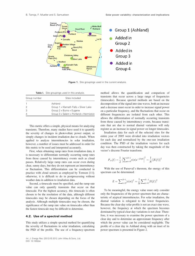
Figure 1. Site groupings used in the current analysis.

Table I. Site groupings used in this analysis.

Group number Sites included

1 Ashland2 Group 1+Klamath Falls +Silver Lake3 Group 2+Burns +Eugene4 Group 3+Salem+Portland+Hermiston


This metric offers a simple, physical means for analyzingtransients. Therefore, many studies have used it to quantifythe severity of changes in photovoltaic power output, orsimply changes in incident irradiation due to clouds. Whenapplied to analyze intermittencies in solar irradiation,however, a number of issues must be addressed in order forthis metric to be used and interpreted accurately.

First, when obtaining ramp rates from irradiation data, itis necessary to differentiate normally occurring ramp ratesfrom those caused by intermittency events such as cloudpasses. Relatively large ramp rates can occur even duringclear, sunny days, but they do not represent an intermittencyor fluctuation. This differentiation can be conducted inpractice with cloud sensors as employed by Tomson [11];otherwise, it is difficult to do in postprocessing withoutweather data in addition to irradiation data.

Second, a timescale must be specified, and the ramp ratevalue can only quantify transients that occur on thattimescale. For the highest accuracy, this timescale is oftenchosen to be the resolution of the data, although differenttimescales may be chosen depending on the focus of theanalysis. Although multiple timescales may be chosen, thesignificance of the ramp rate value on timescales other thanthe fastest timescale may be difficult to determine.

4.2. Use of a spectral method

This study utilizes a simple spectral method for quantifyingthe severity of fluctuations in solar irradiation, calculatingthe PSD of the profile. The use of a frequency-spectrum


method allows the quantification and comparison oftransients that occur across a large range of frequencies(timescales). Because spectral methods are based on thedecomposition of the signal into sine waves, both an increaseand a decrease must occur in order to increase signal poweron a particular frequency, and the fluctuations that occur ondifferent frequencies are isolated from each other. Thisallows the differentiation of normally occurring transientsfrom those caused by intermittency events, because transi-ents that are due to normal diurnal variations will onlyregister as an increase in signal power on longer timescales.

Irradiation data for each of the selected sites for theentire year of 2005 were divided into irradiation vectorsfor each day and normalized by the one-sun irradiationcondition. The PSD of the irradiation vectors for eachday was then constructed by taking the magnitude of thevector’s discrete Fourier transform:

Pxx fð Þ ¼ 12�XN-1

n¼0x nð Þe�j2pfn

��2¼ 1

NX fð Þk k2

With the use of Parseval’s theorem, the energy of thisspectrum can be determined:

E ¼XN-1

n¼0x nð Þj j2 ¼ 1

N

XN�1

n¼0X fð Þj j2

To be meaningful, the energy value must only consideronly the frequencies of the power spectrum that are charac-teristic of atypical intermittencies. For solar irradiation, thediurnal variation is relegated to the lower frequencies.Because the clear-day solar profile is not an exact sine wave,however, the frequency at which the spectrum becomesdominated by typical clear-day variations is not clear. There-fore, it was necessary to examine the power spectrum of aclear day and to determine an approximate frequency afterwhich the power value can be considered negligible. Theprofile of a clear day in Ashland along with an inset of itspower spectrum is presented in Figure 2.

Figure 2. Clear-day irradiation profile and corresponding power spectrum.


The value of the power spectrum for this clear day nomi-nally reaches zero at a frequency of approximately 400mHz,corresponding to a timescale of 0.7 h or 42min. At higherfrequencies, the value of the spectrum remains very lowcompared with that of the frequency components lower thanthis value. Note, however, that the criterion for determiningwhether the power value at a given frequency is negligibleis somewhat arbitrary. For this study, the frequency wherethe value of the spectrum dropped below 5(10-8) times themaximum value of the clear-day spectrum was determinedto be the dividing frequency. A different ratio can be usedif this method is utilized as long as the calculated energyvalue does not include significant contributions from spec-trum components that arose because of normal clear-dayvariation in solar irradiation while still capturing variationsthat occur on the timescale range of interest. Note that,because the dividing frequency is the lower bound of theportion of the spectrum used in calculating the signal energy,only transients that occur on frequencies equal to or higherthan this will be captured. This must also be consideredwhen determining the appropriate dividing frequency for agiven analysis.

The energy value for the ‘intermittent’ part of the powerspectrum is determined by integrating the spectrum fromthe established lower bound frequency to the highestfrequency allowed by the resolution of the data. For aclear-day profile as displayed in Figure 2, the correspondingspectrum has near-zero values over the domain of integration;

therefore, its energy value is very low in this case (0.285 J).Conversely, for a day that exhibits an irradiation profile withmultiple fluctuations of high magnitude on short timescales,the spectrumwill exhibit very high values over the domain ofintegration, and the corresponding energy value will be veryhigh, as shown for a day in Ashland in Figure 3.

The corresponding spectrum is significantly differentfrom that of the clear day, showing a general change in thelocation of peaks as well as significant signal power valuesover the domain of integration, yielding a high energy valueof 5112.9 J. Even though the portion of the spectrum belowthe dividing frequency is changed, it is difficult to determinewhether the contributions in these frequencies are due tointermittencies or normal clear-day variations; therefore, thisportion is not included in the calculation of the energy value.

The energy value for the appropriate subsection of thepower spectrum is calculated for each day, site, and group-ing, and the magnitude as well as the yearly distribution ofthe energy value is used as the metric for quantifying andcomparing the severity of solar intermittencies. As the irradi-ation profile of a single day exhibits an increasing amount ormagnitude of fluctuations because of factors other than thetypical diurnal variation (such as cloud passes), the energyvalue of the spectrum subsection increases. This trend wasdiscovered to be consistent for all of the days of the year.

Overall, a simple method based on Parseval’s theoremhas been developed to quantify solar intermittency acrossa range of timescales and allows the separation of normally


Figure 3. Irradiation profile of a highly transient day and corresponding power spectrum.


occurring changes in irradiation from changes caused byundesirable intermittency events such as cloud passes.Note that the accuracy of this method is highly dependenton the resolution of the data set in question, as using datawith a low temporal resolution can mask the presence offast transients. This work will base its results on a 5-minresolution, which is the highest resolution available fromthe source data, although it is important to note that itmay be possible for solar irradiation dynamics to occuron shorter timescales.

5. SPATIAL DIVERSIFICATION OFSOLAR FARMS AND EFFECTS ONINTERMITTENCY

5.1. Effect of regional solar farm portfoliodiversification on solar profile

This section examines the effect of the spatial diversifica-tion of the deployment of solar farms on the severity ofthe irradiation (and therefore power output) fluctuationsexhibited by the aggregated solar profile. This conceptcan apply to either the distribution of a given solar powercapacity or the successive addition of solar farms at adiverse array of sites that serves a larger area of the elec-tric grid. The sites are aggregated together in groups asdisplayed in Figure 1.


The irradiation profiles used for comparison are normal-ized by one-sun conditions and by the number of sitesincluded. For example, the irradiation profile for one site(Group 1) is created by normalizing the irradiation vectorby 1000W/m2 multiplied by the number of sites. Theirradiation profile for a group of three sites, such as Group2, is created by summing the irradiation vectors for each siteat every time step and by normalizing the resulting vectorby three times the one-sun condition, or 3� (1000W/m2).In general, for each time step,

Gn ¼XNs

i¼1Gi

� �=Ns

where Gn is the normalized irradiation, Gi is the raw irradi-ation value of site i, and Ns is the number of sites included.This normalization is carried out in order to render theprofiles comparable and operates under the assumption thata group of solar farms that cover larger land areas will servea larger, appropriately scaled portion of the load on theelectric grid. The object of examination is the magnitudeof power fluctuations that a solar farm or group of solarfarms will impart onto the electric grid as a fraction oftotal system size, even though for higher solar capacities,the absolute magnitude of the fluctuations (MW) may beincreased. Finally, all of the sites are assigned an equalweighting: each site contributes equally to the aggregateprofile. The normalized solar profiles of the different


groups for the most transient day of Group 1 are presentedin Figure 4.

As more sites are added to the total profile, the aggregatenormalized profile becomes smoother in comparison withthe one-site case. Dispersing the farms of the aggregateprofile across large distances appears to decrease the magni-tude of the fluctuations in the normalized profile, as well asslightly altering the shape. The energy values correspondingto each of the profiles are also displayed and are shown todrop considerably as more sites are added to the solar farmportfolio, decreasing by more than an order of magnitudein the transition from Group 1 (5119.2 J) to Group 4(372.4 J). This effect appears to be due to two maindriving forces.

First, because all of the groups with the exception of thefirst are composed of an aggregation of sites, the influenceof the fluctuations occurring at a single site on the aggre-gate profile is reduced as more sites are added. For the caseof Figure 4, the Ashland site experienced severe transientsin incident irradiation, whereas other sites in the state didnot. Therefore, when aggregated with the other sites, theeffect of the Ashland fluctuations was reduced by a factorof 3, 5, and 8 for Groups 2, 3, and 4, respectively. Second,it was found that the fluctuations at different sites did nottend to occur in tandem. When one site experienced asevere positive ramp rate, another site included within thesame group experienced either a very low ramp rate or anegative ramp rate that counterbalanced the behavior ofthe transient site.

Figure 4. Normalized solar profiles for Day 156 of (a) G

Overall, these effects only amount to reducing themagnitude of the fluctuations that appear in the normalizedprofile. These effects do not remove the occurrence ofthese fluctuations, except in the rare cases where exactcounterbalancing occurs. Additionally, these effects aremade possible because the fluctuations that occur at sitesthat are spaced a sufficient distance apart are decoupled.This will be further discussed in a later section.

The behavior exhibited by the most transient day (Day156) was found to be consistent with all other days of theyear. The distribution of the daily energy values for differ-ent individual sites is presented in Figure 5, and that for thesuccessive groupings is presented in Figure 6:

The energy value distributions are presented by way ofa modified histogram. Each figure plots the number of days(horizontal axis) that the energy value is equal to or abovea certain value (vertical axis). For example, the Hermistonsite exhibits approximately 100 days out of the year wherethe energy value is equal to or greater than approximately260 J, as indicated by the red dot and dashed lines inFigure 5(b). The point where the curve reaches the verticalaxis is representative of the energy level of that site orgroup’s highest energy level day. Of the four sitesdisplayed in Figure 5, the Hermiston site, followed by theAshland site, exhibits the lowest energy levels overall.

The energy levels drop significantly as more sites areadded to the farm portfolio. The largest decrease occurs inthe transition from a single site (Group 1) to three sites(Group 2), with slightly diminishing decreases as more sites

roup 1, (b) Group 2, (c) Group 3, and (d) Group 4.


Figure 5. Daily energy value distributions for different individual sites: (a) total and (b) inset.

Figure 6. Daily energy value distributions for site groupings: (a) total and (b) inset.


are added thereafter. The energy level of the worst day dropsfrom 5119.2 to 372.9 J in the transition from Group 1 toGroup 4, and in this particular case, the day with the highestenergy value remains Day 156. All of the multisite groupsexhibit energy levels that are lower than any of the individualsites alone. In general, the number of days that exhibitshigher energy levels decreases as more sites are added, indi-cating that the severity of the fluctuations in the normalizedirradiation profile of each group is reduced.

5.2. Solar irradiation dynamics andimplications for load balancing uncertainty

5.2.1. Uncertainty band and installed regulationcapacity

The short timescale fluctuations exhibited by intermittentrenewable energy sources such as wind or solar have impli-cations for how supporting generators on the grid such asgas turbines must operate to ensure that the load is balancedat all times. The inability to predict solar irradiation at shortertimescales with the accuracy needed for exact load balancingimplies that an increase in the required capacity on the regu-lation market will be necessary to handle the increaseduncertainty in the balance power that will arise withincreased solar penetration. Therefore, it is of interest toexamine the uncertainty associated with these fluctuationsand their sensitivity to effects such as spatial diversification.

The normalized solar profiles of each of the differentgroupings are presented in Figure 7, overlaidwith 1-h averageddata and maximum uncertainty bounds.


For this case, the degree of uncertainty will be explainedin terms of a set of parameters for ease of interpretation. Thequantity ‘l’ is defined as the magnitude of the deviation insolar irradiation from the 1-h average. This quantity waschosen because it is expected that the solar irradiation on a1-h timescale can be predicted with reasonable accuracyahead of time; therefore, the fluctuations from this averagewill determine the profile that must be directly met by regu-lation power. The lower bound of the uncertainty band isdetermined by subtracting the magnitude of the largestnegative l value from the 1-h average, whereas the upperbound is determined by adding the magnitude of the largestpositive l value to the 1-h average. The width of the uncer-tainty band (Λ) is defined as the width of the band formed bythe upper and lower bounds for each day. This metric isnominally representative of the regulation capacity requiredto ensure that the total load demand is always balanced bytotal generation, because there must be enough regulationor ramping capacity scheduled ahead of time to mitigatethe largest fluctuations that may occur during a given day.The maximum positive fluctuation from the 1-h average isthe amount that variable generators on the grid must be ableto turn down in power for that day. The maximum negativefluctuation from the 1-h average is the amount of power thatvariable generators must be able to increase to for that givenday. The range spanned by the two indicates the total operat-ing range of the variable generators, that is, the requiredregulation capacity for that day. Day 156 is used as the primeexample because it exhibits the most severe transients. Thediscussion is given in terms of power rather than irradiation,

Figure 7. Solar profiles of different spatial aggregations with maximum uncertainty bands for Day 156.

Figure 8. Distribution of daily Λ for different spatial aggregations.


because solar power is directly proportional to incident solarirradiation.

With only a single site, the amount of uncertainty in totalpower generation can be very large. In this particular case,the width of the uncertainty band of the normalized solarprofile exceeds a value of 1, indicating that the regulationcapacity that exceeds the rated capacity of the solar systemmust be scheduled to guarantee that loads will be met. There-fore, the installation of solar power in this case does notoffset any amount of required balance generation capacity.

As more sites are added to the portfolio, however, thewidth of the uncertainty band decreases. In transitioningfrom a single site (Group 1) to eight geographically spacedapart sites (Group 4), the width of the uncertainty banddecreases from 104% to 40% of the system’s rated capacity.This transition also shows the largest decrease, consistentwith trends displayed prior, indicating that the regulationcapacity required to compensate for power fluctuations as afraction of total system capacity is reduced. This is due tothe same reasons previously discussed: decreasing theinfluence of fluctuations that occur at individual sites andthe tendency of fluctuations exhibited by individual sitesdo not occur in tandem. This indicates that a main benefitof utilizing a spatially diverse solar farm portfolio is tobuffer the total effect of cloud-induced intermittencies onthe electric grid. Practically, this indicates that very largeamounts of energy storage may not be necessary to buffercloud intermittency if solar farms are spatially diversified.Spatial diversification can allow an initial reduction in therequired capacity or capabilities of auxiliary systems such

as energy storage as a fraction of the total generation capacityor total load demand.

The width of the uncertainty band (Λ) was calculatedfor each day of the year for each of the profiles and ispresented by a modified histogram in Figure 8.

The distribution is presented in a manner similar toFigure 5 and plots the total number of days that themaximum daily Λ of the normalized solar profile is equalto or above a certain value. As more sites are added, thenumber of days exhibiting higher maximum daily Λ isdecreased, showing that the decrease in the width of theuncertainty band that occurs with spatial aggregation tendsto occur as a whole and not only on select days. The largest



decrease in the number of days with a wide uncertainty bandoverall also occurs during the first transition from Group 1 toGroup 2, consistent with the trends presented prior.

From a grid design standpoint, the maximum yearly Λexhibited throughout the year is tied to the amount ofregulation capacity that must be installed on the grid (as afraction of nameplate solar capacity), such that all fluctua-tions in the remaining load demand profile after intermittentpower generation profile has been subtracted can be met.Therefore, in this study, the maximum yearly Λ is referredto as the maximum solar power fluctuation (Psf,max). Thismetric helps quantify the highest amount of variability dueto solar power that the electric grid infrastructure will haveto be capable of accommodating. The behavior of thisquantity with solar penetration level can provide someinsights into the scalability of solar power in terms of integra-tion onto the electric grid and is presented for the case ofsolar penetration in Oregon for solar profiles of differentspatial diversity levels in Figure 9. Therefore, if the solarcapacity required to reach a given level of solar penetrationis installed, the requirements to manage the fluctuations fromthat capacity of solar power from a diverse portfolio of sitesas opposed to installing the entire capacity at a single site canbe evaluated.

As the desired solar penetration level increases, Psf,maxincreases in a linear fashion. This linear trend is onlyapplicable, assuming that no curtailment of solar poweroccurs. Because peak solar power tends to occur in closetemporal proximity to the times of high load demand,however, curtailment will not be an issue at low solar pene-tration levels. Determining the appropriate penetration levelrange with different grid resource mixes is the subject offuture work.

This implies that for a given desired solar penetrationlevel, the amount of regulation capacity that the electricgrid must devote to managing all of the solar irradiationtransients for the year can be decreased if the solar portfo-lio is composed of a larger amount of solar sites. Forexample, suppose that the electric grid system for a given

Figure 9. Maximum solar power fluctuation versus solarpenetration level for Oregon using solar profiles of different

spatial diversity levels.


balancing region (in this case, the state of Oregon) is ableto accommodate only 4000MW of regulation capacityfor managing solar power transients. This capacity wouldbe sufficient to balance the intermittencies of a solar capac-ity equivalent to a 12% solar penetration level if all of thesolar power was produced from one site, whereas a solarpenetration level of 31% can be balanced if eight sites wereused. This is the direct implication of the decreased vari-ability (as a fraction of total system capacity) that comeswith the increased spatial diversification of solar powerinstallations. Spatial diversification of solar power installa-tions allows a larger capacity of solar power to be ac-commodated on the electric grid for a given amount ofdedicated regulation capacity for managing renewable in-termittency. This indicates that spatial diversification canpartially mitigate an obstacle that has hindered the scalingup of the solar power capacity on the grid.

Because Psf,max behaves linearly with desired solarpenetration level in the absence of power curtailment, theeffect of spatial diversity can be examined by calculatingthe slope of the curves presented in Figure 9 as a functionof the number of sites composing the solar profile, aspresented in Figure 10.

As implied by the previous results, the rate of increase ofPsf,max per percent solar penetration decreases as the solarfarm portfolio is composed of a larger amount of sites (i.e.,greater diversity). The largest decrease occurs when transi-tioning from one site to two sites (65MW/%), and smallerdecreases are garnered thereafter. As the number of sites isincreased, the slope of Psf,max with solar penetrationlevel appears to follow a decreasing exponential trend.This behavior makes sense because as single sites areincrementally added to the solar farm portfolio, the recentlyadded site has a smaller effect on the aggregate power signalfor solar farm portfolios that are already spatially diversebecause its contribution is a smaller fraction of the totalpower. This trend assumes that the nameplate power capacityof each of the different sites is equal and may becomedifferent should the weighting of solar power capacitychange between the sites.

Figure 10. Slope of maximum solar power fluctuation–solarpenetration curves versus number of sites.

Figure 11. Coherence spectrum of the Ashland–Hermistonsite pair.


Overall, the spatial diversification of a solar farm port-folio reduces the magnitude of the fluctuations in solarpower as a fraction of the total rated capacity. The energylevels of the short timescale fluctuations in irradiation arereduced as more sites are added, indicating a reduction inthe overall magnitude and amount of occurrences of thesefluctuations. The amount of uncertainty in solar powergeneration that must be prepared for in order to ensureexact load balancing is reduced significantly, implying adecrease in the required regulation capacity in comparisonwith a single-site case. As more sites are added to the solarfarm portfolio, the magnitude of the maximum solar powerfluctuation per percentage increase in solar penetrationlevel decreases, following an inverse exponential trendwith the number of sites composing the solar portfolio.This implies a decrease in the installed regulation capacityneeded to balance solar power fluctuations. This effectallows higher solar penetration levels to be reached for agiven amount of installed regulation capacity or a reduc-tion in the required capabilities of other auxiliary systemssuch as energy storage on the electric grid.

These effects arose because of two principal drivingforces: (i) the reduction in the influence of fluctuations atan individual site from affecting the aggregate and (ii)cloud-induced fluctuations of sufficiently spaced sites arenot simultaneous. This second driving force is examinedin detail herein by the use of the coherence function.

5.2.2. Coherence analysisThe coherence function for two signals x and y is

defined as a ratio of PSDs:

gxy ¼Gxy fð Þ�� 2

Gxx fð Þ�Gyy fð Þ

where Gxy is the cross spectral density as a function offrequency of the two signals and Gxx and Gyy are the PSDsas a function of frequency of the individual signals. Thecoherence function is a real-valued function that gives anindication of how correlated two signals are as a functionof frequency, bounded between 0 and 1, with a value of1 indicating that two signals vary perfectly in tandem onthat particular frequency. This is a useful measure for de-termining whether the variations in irradiation that occurat different sites tend to happen in tandem at a givenfrequency.

The coherence spectrum of one solar site pair, theAshland and Hermiston sites, is displayed in Figure 11.

Although only the coherence spectrum of the Ashland–Hermiston site pair is displayed, this plot is representativeof the coherence spectra of all of the site pairs. The coherencespectrum was calculated using pairs including the Ashlandsite in combination with each of the other sites considered.

The irradiation profiles tend to be correlated to a reason-able degree only on the lower frequencies (longer time-scales). The frequency that exhibits the highest coherencevalue (~0.99+) for the site pairs considered is approximately

11.40mHz, which corresponds to about a 24-h timescale.This makes sense because variations on this timescale aregoverned by the diurnal variation of the sun’s position inthe sky relative to the site in question, which affects all ofthe sites simultaneously. Above a certain frequency, how-ever, the coherence value for the different site pairs dropssignificantly (to less than 0.2). Distinct peaks in coherenceoccur at frequencies of 11.40mHz (1 day), 22.81mHz(12h), 34.21mHz (8 h), 45.62mHz (6 h), and 58.65mHz(4.8 h) for all site pairs, although the peaks that occur at thelatter frequency tend to exhibit low coherence values: about0.4 for the nearest site to Ashland (Klamath Falls) to 0.18for the farthest site from Ashland (Hermiston). Thesepeaks occur because the longer timescale variations are dueto diurnal effects or storm events that can affect sitessimultaneously.

At frequencies higher than 58.65 mHz, the coherencespectra of the different site pairs exhibit no particularpattern in terms of distinct peaks occurring at particularfrequencies or high coherence values. The value of thecoherence function at these faster frequencies tends toremain at a very low value, generally never rising above0.1 and strictly never rising above 0.2. This indicates thatthe short timescale fluctuations in irradiation that a givensite exhibits are not coupled with the similar events occur-ring at a different site.

This result is only reasonable given that the sites inquestion are spaced a sufficient distance apart. The shorttimescale variations are generally caused by the passing ofbroken or scattered cloud patterns over a site. The timescaleof an individual fluctuation in irradiation depends on theamount of time that a particular cloud is covering the siteand is dependent on the size and velocity of the cloud passingover the site or panel array. If the cloud in question movesvery slowly or is very large, the timescale of the fluctuationwill be long and vice versa. The magnitude of an individualfluctuation depends on the size of the cloud relative to theland area covered by the array at any given time. If the cloudin question covers a larger fraction of the array area, theassociated drop in power output will be larger. For the


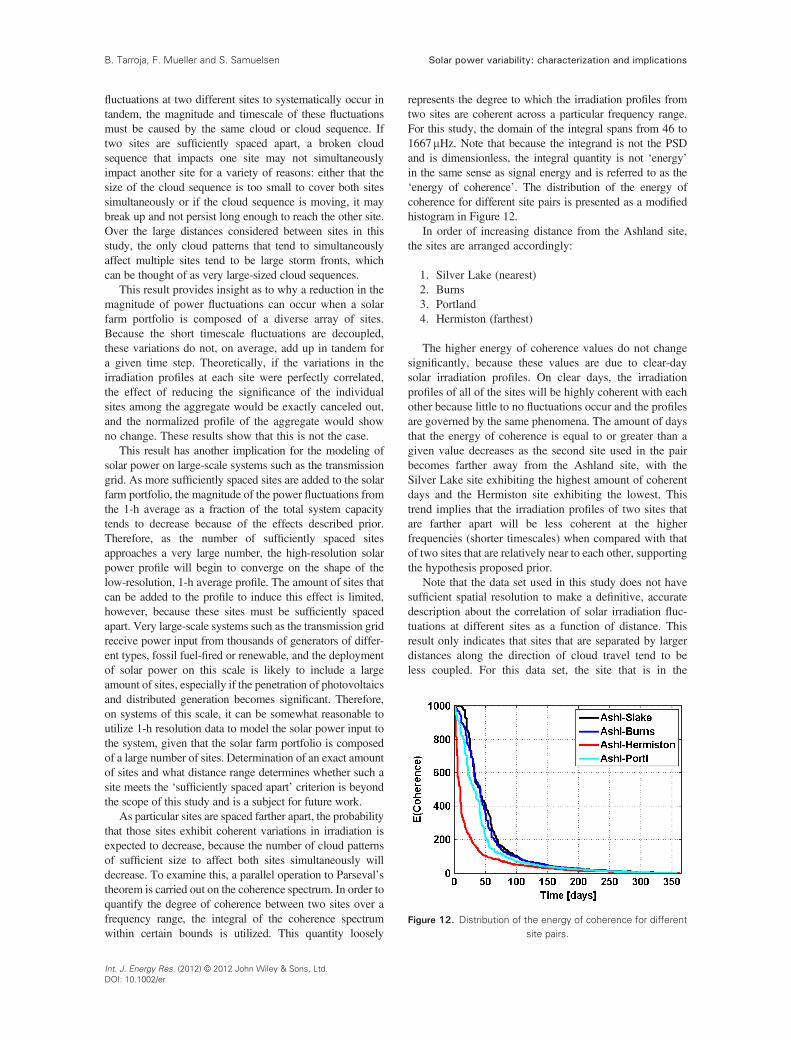
Figure 12. Distribution of the energy of coherence for differentsite pairs.


fluctuations at two different sites to systematically occur intandem, the magnitude and timescale of these fluctuationsmust be caused by the same cloud or cloud sequence. Iftwo sites are sufficiently spaced apart, a broken cloudsequence that impacts one site may not simultaneouslyimpact another site for a variety of reasons: either that thesize of the cloud sequence is too small to cover both sitessimultaneously or if the cloud sequence is moving, it maybreak up and not persist long enough to reach the other site.Over the large distances considered between sites in thisstudy, the only cloud patterns that tend to simultaneouslyaffect multiple sites tend to be large storm fronts, whichcan be thought of as very large-sized cloud sequences.

This result provides insight as to why a reduction in themagnitude of power fluctuations can occur when a solarfarm portfolio is composed of a diverse array of sites.Because the short timescale fluctuations are decoupled,these variations do not, on average, add up in tandem fora given time step. Theoretically, if the variations in theirradiation profiles at each site were perfectly correlated,the effect of reducing the significance of the individualsites among the aggregate would be exactly canceled out,and the normalized profile of the aggregate would showno change. These results show that this is not the case.

This result has another implication for the modeling ofsolar power on large-scale systems such as the transmissiongrid. As more sufficiently spaced sites are added to the solarfarm portfolio, the magnitude of the power fluctuations fromthe 1-h average as a fraction of the total system capacitytends to decrease because of the effects described prior.Therefore, as the number of sufficiently spaced sitesapproaches a very large number, the high-resolution solarpower profile will begin to converge on the shape of thelow-resolution, 1-h average profile. The amount of sites thatcan be added to the profile to induce this effect is limited,however, because these sites must be sufficiently spacedapart. Very large-scale systems such as the transmission gridreceive power input from thousands of generators of differ-ent types, fossil fuel-fired or renewable, and the deploymentof solar power on this scale is likely to include a largeamount of sites, especially if the penetration of photovoltaicsand distributed generation becomes significant. Therefore,on systems of this scale, it can be somewhat reasonable toutilize 1-h resolution data to model the solar power input tothe system, given that the solar farm portfolio is composedof a large number of sites. Determination of an exact amountof sites and what distance range determines whether such asite meets the ‘sufficiently spaced apart’ criterion is beyondthe scope of this study and is a subject for future work.

As particular sites are spaced farther apart, the probabilitythat those sites exhibit coherent variations in irradiation isexpected to decrease, because the number of cloud patternsof sufficient size to affect both sites simultaneously willdecrease. To examine this, a parallel operation to Parseval’stheorem is carried out on the coherence spectrum. In order toquantify the degree of coherence between two sites over afrequency range, the integral of the coherence spectrumwithin certain bounds is utilized. This quantity loosely


represents the degree to which the irradiation profiles fromtwo sites are coherent across a particular frequency range.For this study, the domain of the integral spans from 46 to1667mHz. Note that because the integrand is not the PSDand is dimensionless, the integral quantity is not ‘energy’in the same sense as signal energy and is referred to as the‘energy of coherence’. The distribution of the energy ofcoherence for different site pairs is presented as a modifiedhistogram in Figure 12.

In order of increasing distance from the Ashland site,the sites are arranged accordingly:

1. Silver Lake (nearest)2. Burns3. Portland4. Hermiston (farthest)

The higher energy of coherence values do not changesignificantly, because these values are due to clear-daysolar irradiation profiles. On clear days, the irradiationprofiles of all of the sites will be highly coherent with eachother because little to no fluctuations occur and the profilesare governed by the same phenomena. The amount of daysthat the energy of coherence is equal to or greater than agiven value decreases as the second site used in the pairbecomes farther away from the Ashland site, with theSilver Lake site exhibiting the highest amount of coherentdays and the Hermiston site exhibiting the lowest. Thistrend implies that the irradiation profiles of two sites thatare farther apart will be less coherent at the higherfrequencies (shorter timescales) when compared with thatof two sites that are relatively near to each other, supportingthe hypothesis proposed prior.

Note that the data set used in this study does not havesufficient spatial resolution to make a definitive, accuratedescription about the correlation of solar irradiation fluc-tuations at different sites as a function of distance. Thisresult only indicates that sites that are separated by largerdistances along the direction of cloud travel tend to beless coupled. For this data set, the site that is in the


closest proximity to the Ashland reference site is KlamathFalls, which is still approximately 70miles away. Thecoherence spectrum of the Ashland–Klamath Falls pairtends to show slightly higher coherence values than sitesthat are further away at the distinct frequencies mentionedprior, but that is not enough to create an expression thatmodels the degree of coherence as a function of distanceand direction. Such an expression will require an under-standing of regional weather patterns and a higher spatialresolution and is a topic for future work.

5.2.3. Discussion: solar variability and thetransmission system

The short timescale fluctuations of solar power have thepotential to affect not only the balancing of the bulk loaddemand but also the management of power flow within a

Figure 13. Combination of power flow from three solar farms.

Figure 14. Interconnection of three solar fa

balancing area and between different balancing areas(power imports and exports). This section discusses theimplications of solar power variability for electric gridoperations that occur within and between balancing areas.

In order for the full smoothing effect of the spatialdiversification of solar farms to be realized by othergenerators on the grid, the power flow from the individualfarms are combined with each other before being transmit-ted to serve a load center. With this arrangement, the shorttimescale fluctuations in solar power output will bereduced before being imposed on a load center or balanc-ing generator. A schematic of this arrangement is shownin Figure 13.

The interconnection of solar farms in the manner shownin Figure 13 is not always feasible, however. Because thesolar farm portfolio will be spatially diverse, the solarfarms will most likely be located far away from each other,and power flow from each farm may not be able tocombine with each other to create a smooth power signal.For example, power flow from a single solar farm maybe directed toward serving a load center that is located inclose proximity without having directly combined withpower flows from other solar farms. In this case, thesubstation and local balancing generators will locallyobserve the full magnitude of power output variation froma single solar farm, even though many solar farms areinstalled throughout the entire balancing area. A schematicof this arrangement, which more closely represents a solarinterconnection scenario, is presented in Figure 14.

Therefore, it is of key importance that not only theload balancing aspect of accommodating large amounts

rms with loads within a balancing area.



of solar power on the electric grid but also the designand operation of the transmission system be addressedsuch that benefits garnered by acts such as spatial diver-sification of solar farms can be realized. This is a subjectfor future work.

6. CONCLUSIONS

A method to quantify the severity of fluctuations in solarirradiation and power output exhibited by a givengeographic site accounting for the different timescales offluctuation has been utilized. The effect of utilizingsolar farm portfolios with increasing levels of spatialdiversification on the magnitude of irradiation or powerfluctuations as a fraction of the total system capacity hasbeen examined and compared with a single-site case as areference. The implications of the effect for balancegeneration have been discussed.

The key conclusions of this study are as follows:

1. The spatial diversification of the solar farm site portfo-lio allows for a reduction in the magnitude of normal-ized irradiation (and therefore power) fluctuations as afraction of the total system capacity installed on theelectric grid. This is due to two effects: (i) the reduc-tion in the influence of fluctuations at one site on theaggregate profile and (ii) the irradiation profilesbetween two sites that are sufficiently spaced apart soas to not be correlated.

2. The degree of variation associated with solar poweroutput as measured by the size of the uncertaintyband is decreased as more sufficiently spaced sitesare added to the total profile.

3. The maximum solar power fluctuation, which is tied tothe amount of regulation capacity that must beinstalled on the electric grid to balance all of the solarpower fluctuations for a given year, is decreased asthe solar farm portfolio becomes increasingly diverse.This indicates that higher solar penetration levels are tobe reached for a given amount of installed regulationcapacity or lower required increases in installed regu-lation capacity per unit increase in solar penetrationlevel. The rate of increase in required regulation capac-ity with increases in desired solar penetration leveldecreases in an exponentially decaying manner withthe number of sites composing the solar farm portfolio.

4. The fluctuations in solar irradiation that occur ontimescales faster than 6 h are uncorrelated betweensites that are sufficiently spaced apart. Therefore,the faster fluctuations that occur at each site did notoccur simultaneously and sometimes even counter-balanced each other.

5. Because of the low coherence between sufficientlyspaced apart sites at shorter timescales, it may bereasonable to utilize hourly resolved data to modelsolar power transients on very large-scale systemssuch as the transmission grid, under the condition


that the solar farm portfolio consists of a largeamount of sufficiently spaced apart sites.

Overall, utilizing a spatially diverse solar farm portfolioappears to offer a means of partially mitigating some ofthe disadvantages and concerns with the increased penetra-tion of solar power into the electric generation portfolio ofthe grid: namely issues concerned with the severe unpredict-ability of solar irradiation and associated dynamics. Theimplementation of spatial diversification renders theseconcerns to be more manageable than originally perceivedand has the potential to reduce the required capabilities ofauxiliary systems, which must manage the effect of theseissues such as balance generators or energy storage systems.

On the larger scale, however, novel energy managementstrategies will need to be developed to effectively androbustly utilize solar power along with a diverse portfolioof other renewable energy sources and conventionalsources in order to retain the stability of the electric gridwith increased renewables. In order to develop these strate-gies, it is important to understand what can be done at eachlevel in the electricity generation chain (generation, trans-mission, delivery, and use) to accommodate the behaviorof renewable energy resources. The benefits and deficien-cies of other renewable resources and the analysis of holis-tic approaches to attaining high levels of overall renewablepenetration into the electric grid and to identifying the typesof complexities required to manage renewable powerresources on the grid are the focuses for future work.

ACKNOWLEDGEMENTS

This document was prepared in part as a result of worksponsored by the California Energy Commission underContract No. PIR-08-033. It does not necessarily representthe views of the Energy Commission, its employees, or theState of California. The Energy Commission, the State ofCalifornia, its employees, contractors, and subcontractorsmake no warranty, express or implied, and assume no legalliability for the information in this document; nor does anyparty represent that the use of this information will notinfringe upon privately owned rights. This report has notbeen approved or disapproved by the Energy Commissionnor has the Energy Commission passed upon the accuracyof the information in this report. The authors would alsolike to express their appreciation to the University ofOregon for making irradiation data available in the publicdomain and to the National Science Foundation forsupporting the graduate studies of the lead author throughthe Graduate Research Fellowship Program.

REFERENCES

1. Sherwood L. 2009 Solar Industry Year in Review.Solar Energy Industries Association: Washington DC,2009; 1–12

2. CPUC. California Solar Initiative Program Hand-book. 2010.


3. Hermann WA. Quantifying global exergy resources.Energy 2006; 31(12):1685–1702.

4. NREL.National Solar Radiation Database. Departmentof Energy: U.S., 1991–2005

5. NREL. Concentrating Solar Resource of the UnitedStates. DOE: U.S., 2009.

6. Moharil RM, Kulkarni PS. Reliability analysis of solarphotovoltaic system using hourly mean solar radiationdata. Solar Energy 2008; 84(4):691–702.

7. Ehnberg SGJ, Bollen MHJ. Reliability of a smallpower system using solar power and hydro. ElectricPower Systems Research 2005; 74(1):119–127.

8. Porter K. Intermittency analysis project: final report.California Energy Commission, Public Interest EnergyResearch Program, 2007.

9. Vick B, Clark R, Mehos M. Improved electrical loadmatch in California by combining solar thermal powerplants with wind farms. In 37th ASES Annual Conference.San Diego, CA, 2008.

10. Larraín T, Escobar R, Vergara J. Performance modelto assist solar thermal power plant siting in northernChile based on backup fuel consumption. RenewableEnergy 2009; 35(8):1632–1643.

11. Tomson T. Fast dynamic processes of solar radiation.Solar Energy 2009; 84(2):318–323.

12. Tomson T, Tamm G. Short-term variability of solarradiation. Solar Energy 2006; 80(5):600–606.

13. Vijayakumar G, Kummert M, Klein SA, BeckmanWA. Analysis of short-term solar radiation data. SolarEnergy 2005; 79(5):495–504.

14. Reikard G. Predicting solar radiation at high resolutions:a comparison of time series forecasts. Solar Energy2009; 83(3):342–349.

15. Lave M, Kleissl J. Solar variability of four sites acrossthe state of Colorado. Renewable Energy 2010;35:2867–2873.

16. Mills A. Implications of Wide-Area GeographicDiversity for Short-Term Variability of Solar Power.DOE: Lawrence Berkeley National Laboratory, U.S.,2010.

17. Curtright A, Apt J. The character of power outputfrom utility-scale photovoltaic systems. Progress inPhotovoltaics: Research and Applications 2008;16:241–247.

18. Sørensen B. A sustainable energy future: constructionof demand and renewable energy supply scenarios.International Journal of Energy Research 2008; 32(5):436–470.

19. Sørensen B. A renewable energy and hydrogenscenario for northern Europe. International Journalof Energy Research 2008; 32(5):471–500.

20. Syed AM, Fung AS, Ugursal VI, Taherian H. Analysisof PV/wind potential in the Canadian residential sectorthrough high-resolution building energy simulation.International Journal of Energy Research 2009; 33(4):342–357.

21. Niemi R, Lund PD. Alternative ways for voltagecontrol in smart grids with distributed electricitygeneration. International Journal of Energy Research2011. DOI: 10.1002/er.1865


Documents

Solar Power Variability and Spatial Diversification (2)