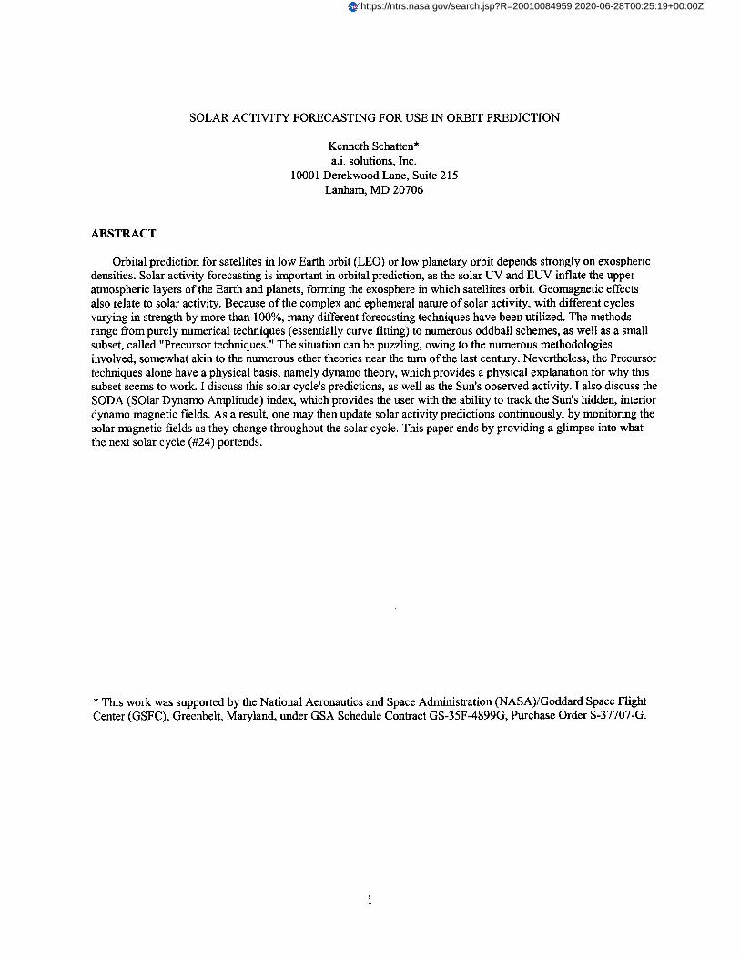
SOLAR ACTIVITY FORECASTING FOR USE IN ORBIT PREDICTION

Kenneth Schatten*

a.i. solutions, Inc.

10001 Derekwood Lane, Suite 215

Lanharn, MD 20706

ABSTRACT

Orbital prediction for satellites in low Earth orbit (LEO) or low planetary orbit depends strongly on exosphericdensities. Solar activity forecasting is important in orbital prediction, as the solar UV and EUV inflate the upper

atmospheric layers of the Earth and planets, forming the exosphere in which satellites orbit. Geomagnetic effectsalso relate to solar activity. Because of the complex and ephemeral nature of solar activity, with different cycles

varying in strength by more than 100%, many different forecasting techniques have been utilized. The methodsrange from purely numerical techniques (essentially curve fitting) to numerous oddball schemes, as well as a smallsubset, called "Precursor techniques." The situation can be puzzling, owing to the numerous methodologies

involved, somewhat akin to the numerous ether theories near the turn of the last century. Nevertheless, the Precursor

techniques alone have a physical basis, namely dynamo theory, which provides a physical explanation for why thissubset seems to work. I discuss this solar cycle's predictions, as well as the Sun's observed activity. I also discuss the

SODA (SOlar Dynamo Amplitude) index, which provides the user with the ability to track the Sun's hidden, interiordynamo magnetic fields. As a result, one may then update solar activity predictions continuously, by monitoring the

solar magnetic fields as they change throughout the solar cycle. This paper ends by providing a glimpse into whatthe next solar cycle (#24) portends.

* This work was supported by the National Aeronautics and Space Administration (NASA)/Goddard Space FlightCenter (GSFC), Greenbelt, Maryland, under GSA Schedule Contract GS-35F-4899G, Purchase Order S-37707-G.

https://ntrs.nasa.gov/search.jsp?R=20010084959 2020-06-28T00:25:19+00:00Z

INTRODUCTION

Thispaperwill focusonlongtermsolaractivitypredictions.I discusswhysolaractivityforecastingisusefulforsatelliteorbitdetermination,andthenconcentrateonsolaractivityforecastingmethods.I shallendthiswitharoughoutlineofhowthe"SOlarDynamoAmplitude"method(SODAindex)isusedtopredictsolaractivity,andalsothephysicalbasisofthesolardynamomethod.Thismethodhaspredicted3solarcyclesquitewell,havingfirstbeentestedwith8priorcyclesofdata.Thepaperbeginswithadiscussionofhowsolaractivityforecastingisusefulforflightdynamics.

SatellitesinlowEarthorbit(LEO)orlowplanetaryorbithavepathsthatdependstronglyon exosphericdensities, since these densities affect satellite drag. Of course, satellite and orbital properties (ballistic coefficient

related to drag vs. mass, orbital properties, etc.) are also important. It is not through the satellite properties, butrather through the variations in the exospheric densities, that solar activity plays a strong role in orbital paths.

Interestingly, the Sun, whose nearly constant energy source provides a very stable harbor for life on Earth,

provides a very unstable environment for satellites in orbit. The reason is that the solar UV and EUV irradiancesvary dramatically with solar activity (showing changes at certain wavelengths of more than 100%), and this energyinflates the upper atmospheric layers of the Earth and planets, forming the exosphere in which satellites orbit. The

solar UV radiation ionizes oxygen, forming ozone in the Earth's stratosphere; and above this, the more intense EUV

forms the hotter thermosphere and exosphere, in which terrestrial satellites orbit. Solar activity energy, as opposed tothe more constant solar luminosity, thus inflates the Earth's atmosphere into its upper layers. These upper layers varyexponentially with the exotic forms of solar radiation, making them more sensitive to the some of the most variable

forms of solar radiation. Hence sateUite drag is greatly magnified by solar activity. Consequently, solar activityforecasting is a valuable tool for orbit predictions. This exospheric behavior contrasts greatly with tropospheric

behavior, where meteorologists traditionally, yet safely, ignore solar irradiance changes. The solar irradiance iscalled as a misnomer, the "solar constant," since its changes are about 0. I%, much smaller than the EUV variations

which often exceed 100%! Let us now examine solar activity behavior and how this is predicted.

Figure 1 shows solar activity as measured by sunspots for the past few centuries. Firstly, the most prominentfeature is the famous 11-year Schwabe solar cycle. Additionally, there is "power" at a variety of other periods

(including days, months, 80 - 100 years, and even secular variations with longer periods not seen here), however, acloser examination of these periods shows that they are no_..Atstrictly periodic. They appear "chaotic;" unable to be

predicted on the basis of simple spectral techniques. Additionally, even the main 11-year periodicity is no_..Ata sharpperiod; some cycles have been as short at 8 years, and some as long as 17 years! Further, the amplitude of the cycles

varies by more than 100%, in a rather chaotic manner. This is even more striking, if one realizes that there were longperiods of time (50 - 100 years), most recently in the 1600's called the "Maunder minimum" when solar activity wasnear 0. Hence solar scientists have developed numerous methods in their attempts to forecast solar activity.

Unfortunately, a number of these techniques, although successful for some cycles, have failed in the long run.

Methods of solar activity forecasting may be placed in general categories. A NASA-funded NOAA panelinvestigating these methods several years ago (see Joselyn et al. l) chose the following general solar forecasting

categories: Even/Odd Behavior, Spectral, Recent Climatology, Climatology, Neural Networks, and Precursors.Briefly, these categories indicate the following:

• Even/Odd Behavior - uses the relationship that this century (see Figure 1), and for most of the last century as

well, the Odd numbered cycles have been larger than the preceding Even Numbered cycles.

• Spectral - analyzing activity by spectral methods, such as Fourier analysis.

• Recent Climatology - simply averaging recent cycles, say the last 5.

• Climatology - using statistics of the longest duration of solar cycles (although usually leaving out the MaunderMinimum) to obtain a mean cycle and standard deviation to obtain a simple mean and uncertainty.

• Neural Networks - using AI - artificial intelligence methods on solar activity.

• Precursors - physical phenomena related to future solar activity levels. The Precursor category has been

subdivided into geomagnetic and solar magnetic branches, since they gave slightly different prediction levelsfor this cycle 2.

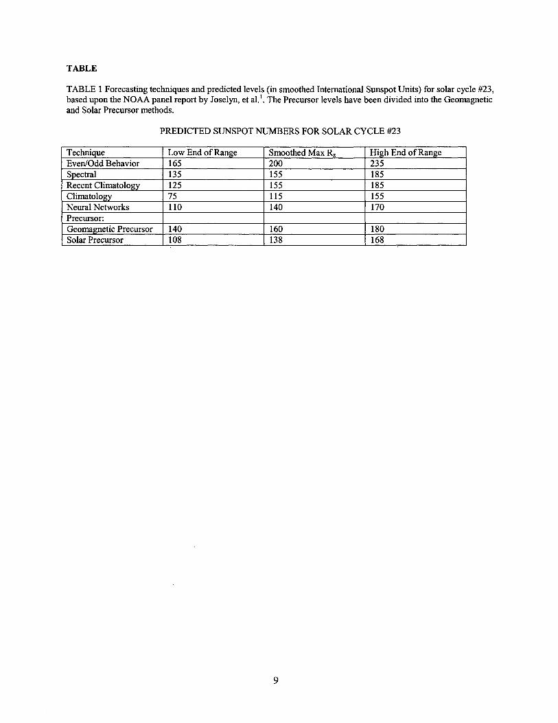
Theabovemethodssuggestthevaluesforsolarcycle#23'ssmoothedpeaksunspot numbers shown in Table 1.

It now appears from the behavior of this cycle that it will peak near a smoothed sunspot number near 125 + 15, or an

F10.7 Radio Flux of 180 + 15. The sunspot value is near the lower end of most estimates seen in Table 1. From an

examination of Table 1, one sees the solar cycle behavior, for this cycle, supports the Climatology, Neural

Networks, and Solar Precursor methods. Geomagnetic Precursors predicted too large a value, partially due to theGeomagnetic Precursors reaching their minimum values late. Additionally, the Even/Odd behavior predicted toolarge a value.

There are other methods that might be added to these categories, such as the McNish-Lincoln method 3, which

although not originally thought to be applicable to predictive capability beyond a year in advance, has been used by

MSFC for longer duration forecasts. It simply is a kind of"curve fitting" technique, with a regression towards amean cycle, and thus is considered in the climatological category. In addition, some have advocated using planetaryorbits, since Jupiter's 11-year period is close to a solar cycle. Hence gravitational changes in the solar system do

correlate for short intervals with solar activity, though any agreement is simply a fortuitous short-lived one.

I shall make a few general comments about these techniques and then concentrate upon Precursor methods,which have been shown to be generally useful over several solar cycles and have a physical basis, as well asstatistical support. As mentioned, the Precursor category may be subdivided into solar and geomagnetic varieties.

This past cycle the solar Precursors suggested a peak value 2 near smoothed sunspot number of 138 + 30 in 1996 and

F 10.7 values of 182 + 30 (Schatten, Myers, and Sofia2). This value was lower than the geomagnetic predictions. Let

us now go through the Table 1 list, and provide some comments about these "traditional" methods.

The first method, Even/Odd, can be seen in the 20 th century of Figure 1, wherein if one numbers the cycles (the

present one is #23), then for this past century all odd numbered cycles have been larger than the preceding even-numbered one. This Even/Odd effect seemed to us like a small statistical fluke. Consider that there have been only4 previous such pairs this century - cycles 14 through 21. If one takes the first pair, one or the other must be larger,

hence one can't count the first pair to support any effect. Hence, there are only 3 matching subsequent pairs, the

chance of these three agreeing with the first is only one in eight, or a significance of 87%, not highly significant! Ifone includes the last cenmry's cycles, one adds 4 more pairs, but only 3 agree with the pattern. Additionally, the

previous pair falls half within the previous century, but this pair disagrees with the Even/Odd effect. This marginallychanges the statistics. Additionally, using this method would suggest that cycle #23 should be the largest cycle ever,it being an odd cycle following the largest even numbered cycle! One is fortunate not to believe in the Even/Odd

effect, using the reason is that there was no physical basis for it because this enormous activity does not appear to behappening!

The second method, Spectral, has seen the most attention throughout the history of solar activity predictions,since Fourier analyses have been readily available, and the methods generally useful for periodic phenomena. In

recent times, however, with new knowledge of "chaotic" systems, it has become generally recognized that Fourier or

generally spectral methods do not lend themselves to understandings of chaotic phenomena. The most obvious areawhere this is seen is in weather prediction. A weather forecaster would not be well received if s/he tried to forecast

the weather at a location on Earth simply by taking parameters at that location and Fourier analyzing them. Thereason, of course, is that knowledge in a chaotic system becomes "lost," whereas in a Fourier or spectral method, the

coefficients are as dependent on what happened recently as on what happened in the distant past. Further,examination of long-term solar activity, using cosmogenic isotopes reveals that commonly accepted cycles (e.g. theGleissberg cycle of 80-100 years), do not bear out over long periods, with significant power in the solar activity

cycle over periods in the few hundred to thousand year range. This would be expected if one considers the "timeconstant" expected for changes, at the base of the convection zone, where magnetic fields are regenerated.

Next, we come to Recent Climatology, and Climatology. These basically, simply use the statistics of known

solar cycles, with climatology using the last few hundred years, from after the Maunder Minimum to present. Oneobtains a mean and standard deviation to get the chances of any size cycle. Recent climatology recognizes the

"chaotic nature" of solar activity, and thus eliminates the early data. One develops a "recent average" and "recentstatistical behavior" from the last few cycles. This method relies strictly upon "persistence," which is at the heart ofthe Precursor methods too, although they have an added physical component. One of the earliest solar activity

prediction methods in this category is the curve fitting techniques of McNish and Lincoln. In this method the recent

behaviorgraduallyblendsintotheaveragebehavior,however,thetechniquewastobeutilizedfornomorethanayearinadvance.

ThenextsetofmethodsisNeuralNetworks-usingAI -artificialintelligencemethodsonsolaractivity.Unfortunately,thesehavebeenusedprimarilyto"curvefit."AlthoughAIcanbeapowerfultechnique,butsince,atpresent,thismethodhasonlybeensuppliedwithpastactivity,aninadequatesourcetopredictfutureactivityfrom,thetechniquesuffersfromaninadequatedatabasetomakelongtermpredictions.Nevertheless,theAI techniqueseemstoprovideacurvefittingtechniquesimilartothatoftheMcNish-Lincolnmethod,whichworksforabout1yearinadvance.Overalongtimeinterval,thismethodrevertstotheclimatologicalmethod,andthusprovideslittlemorethananaverage.ThepapernowdiscussesPrecursormethodsmorefully,distinguishingsolarfromgeomagneticPrecursormethods.Ingeneral,formoreinformationonsolaractivitypredictionmethodsincludingPrecursormethods,theNOAApaneldiscussionsIprovidesanexcellentsource.Further,otherviewsincludingmoredetailonclimatologicalandstatisticalmethodsmaybefoundinHollandandVaughan4,Kerridge, et al: andHathaway, et al. 6.

SOLAR AND GEOMAGNETIC PRECURSOR METHODS

Geomagnetic Precursors

As far as geomagnetic Precursors, one of the first to point out the significance of the geomagnetic Aa index intracking long-term solar activity was Feynman 7. Although she never used the information for directly makingpredictions, it seems clear that Ohl s'9 and other Geomagnetic Precursor practitioners used the same or similar

methods to predict activity. Feynman separated the geomagnetic Aa index into two components: one in phase with

sunspot number, and one out of phase. This effectively led to "active" and "quiet" components. She found that thisquiet signal tracked the sunspot numbers several years in advance, similar to the Ohl results. The maximum in this

signal occurs at sunspot minimum and is proportional to the sunspot number during the following maximum. Howthis signal propagated or why it should be present, however, was not clear.

Precursor methods were developed by the Soviet geophysicist Ohl 8'9to make solar predictions and taken up byBrown and Williams t°, who later noticed an extremely high correlation (close to 1) between geomagnetic activity

near solar minimum and the size of the next solar cycle. High correlations were found between the number of

"geomagnetic abnormal quiet days" and the size of the next solar cycle. Although the abnormal quiet daygeomagnetic index was an unusual one, later the correlations remained high when objective geomagnetic indices,such as Ap, and Aa were employed. Barrels 11discusses these indices. Thompson 12 further improved upon the

relationships between geomagnetically "disturbed" days and the amplitude of the next sunspot maximum.

Let us move on to Precursor methods by pointing out that the correlations found by the geophysicists were very

puzzling because the Sun's activity might cause a terrestrial effect, but not vice versa! So the order of the causalityseemed to be reversed. Trying to unravel the mystery of how the Sun could broadcast to the Earth, in advance, thelevel of its future activity, Schatten et al. 13searched for a physical mechanism to understand the phenomena. To

place these puzzling correlations in a physical context meant relating these geomagnetic effects somehow to solardynamo theory. Let us examine how this is done.

Solar Dynamo Theory and Solar Precursors

In any MHD (magnetohydrodynamics) dynamo, there is a behavior similar to the simple "disk dynamo" shown

in Figure 2. This property is that the amplified magnetic field is proportional to the initial magnetic field. The solardynamo goes through more "gyrations" than the simple disk dynamo, but the previous behavior remains. Figure 3shows the Babcock dynamo, generally agreed upon for the Sun, as there are many observed solar features explained

by this model. Namely, in this model the Sun's polar fields near solar minimum are wrapped up by differentialrotation to form the toroidal fields, which later float to the Sun's surface and erupt to form active regions. As these

fields dissipate, they then regenerate the polar field allowing the solar cycle to recur. Modem helioseismologicalstudies have shed new light on the Sun's dynamo. For example, the solar community now knows that the buried

toroidal dynamo field is located just below the base of the convection zone. Nevertheless, the broad view outlinedby Babcock still remains valid.

4

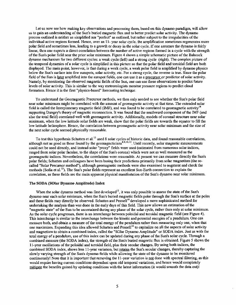
Letusnowseehowmakingkeyobservationsandprocessing them, based on this dynamo paradigm, will allow

us to gain an understanding of the Sun's buried magnetic flux and to better predict solar activity. The dynamoprocess outlined is neither as simplified nor "perfect" as outlined, but rather subject to the irregularities of theindividual active regions formed. Hence, over an 11- year solar cycle, the amplification sometimes regenerates more

polar field and sometimes less, leading to a growth or decay in the solar cycle. If one assumes the dynamo is fairlylinear, then one expects a direct correlation between the number of active regions formed in a cycle with the strength

of the Sun's polar field near the prior solar minimum. Figure 4 shows a simple schematic picture of the Babcockdynamo mechanism for two different cycles: a weak cycle (left) and a strong cycle (right). The complex picture of

the temporal dynamics of a solar cycle is simplified in this picture so that the polar field and toroidal field are bothdisplayed. The main point, however, is that during a weak cycle, a weak polar field is amplified by dynamo physicsbelow the Sun's surface into few sunspots, solar activity, etc. For a strong cycle, the reverse is true. Since the polar

field of the Sun is later amplified into the sunspot fields, one can use it as a precursor or predictor of solar activity.

Namely, by monitoring the observed magnetic fields of the Sun, one can use these observations to predict futurelevels of solar activity. This is similar to the way meteorologists monitor pressure regions to predict cloudformation. Hence it is the first "physics-based" forecasting technique.

To understand the Geomagnetic Precursor methods, we then only needed to see whether the Sun's polar field

near solar minimum might be correlated with the amount of geomagnetic activity at that time. The extended solarfield is called the Interplanetary magnetic field (IMF), and was found to be correlated to geomagnetic activity 14

supporting Dungey's theory of magnetic reconnection. It was found that the southward component of the IMF (andalso the total field) correlated well with geomagnetic activity. Additionally, models of coronal structure near solarminimum, when the low latitude solar fields are weak, show that the polar fields arc towards the equator to fill the

low latitude heliosphere. Hence, the correlation between geomagnetic activity near solar minimum and the size of

the next solar cycle seemed physically reasonable.

To test this hypothesis Schatten et al. 13used 8 solar cycles of historic data, and found reasonable correlations,

although not as good as those found by the geomagneticians 8'9'1°'12.Until recently, solar magnetic measurementscould not be used directly, and instead solar "proxy" fields were used (estimated from numerous solar indices,

ranged from solar polar faculae, to the shape of the Sun's corona) which were not as well measured as thegeomagnetic indices. Nevertheless, the correlations were reasonable. At present we can measure directly the Sun's

polar fields; Schatten and colleagues have been basing their predictions primarily from solar magnetism (the so-called "Solar Precursor method"), although geomagnetic methods were also examined to augment and check themethods (Sofia et al._5). The Sun's polar fields represent an excellent Sun-Earth connection to explain the

correlation, as these fields are the main apparent physical manifestation of the Sun's dynamo near solar minimum.

The SODA (SOlar Dynamo Amplitude) Index

When the solar dynamo method was first developed _3, it was only possible to assess the state of the Sun's

dynamo near each solar minimum, when the Sun's buried magnetic fields poke through the Sun's surface at the polesand these fields may directly be observed. Schatten and Pesnel116 developed a more sophisticated method for

undertaking the analysis than was done in the early days of this field. This now allows an estimation of the"magnetic state" of the Sun to be ascertained during any phase of the solar cycle, rather than only at solar minimum.As the solar cycle progresses, there is an interchange between poloidal and toroidal magnetic field (see Figure 4).

This interchange is similar to the interchange between the kinetic and potential energies of a pendulum. One canmeasure both, and obtain a measure of the total energy of the pendulum rather than measuring only one, when that

one maximizes. Expanding this idea allowed Schatten and Pesnell t6 to capitalize on all the aspects of solar activityand magnetism to obtain a combined index, called the "SOlar Dynamo Amplitude" or SODA index. Just as with the

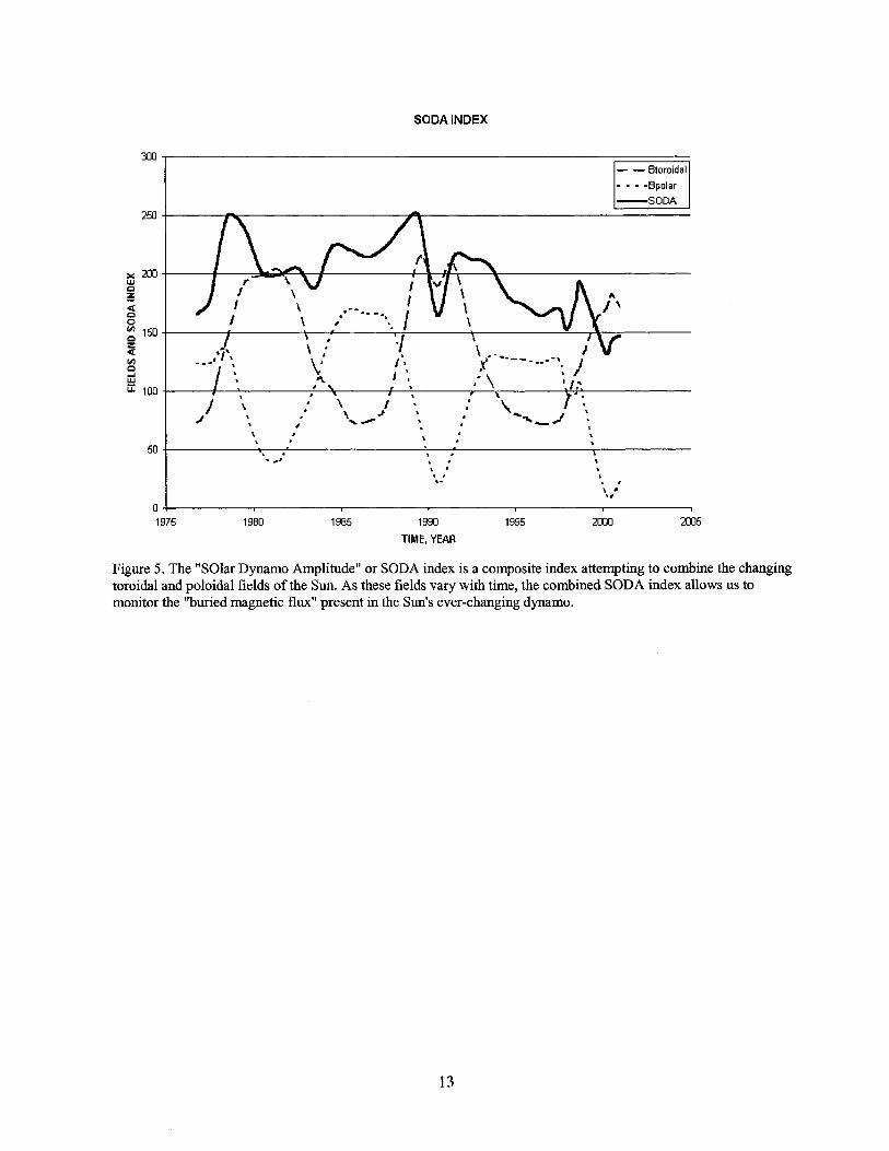
total energy of a pendulum, use of this index can be updated during any phase of the Sun's solar cycle. Through acombined measure (the SODA index), the strength of the Sun's buried magnetic flux is obtained. Figure 5 shows the

11-year oscillations of the poloidal and toroidal field, plus their secular changes. By using both indices, thecombined SODA index, shows less 11-year variation, but retains the Sun's secular changes, thereby capturing the

slowly varying strength of the Sun's dynamo fields while allowing the state of the dynamo to be monitoredcontinuously! Note that it is important that removing the 11-year variation is not done with spectral filtering, as thiswould require having current conditions dependant upon old temporal variations, and hence would completely

mitigate_ the benefits gained by updating conditions with the latest information (it would smooth the data out)!

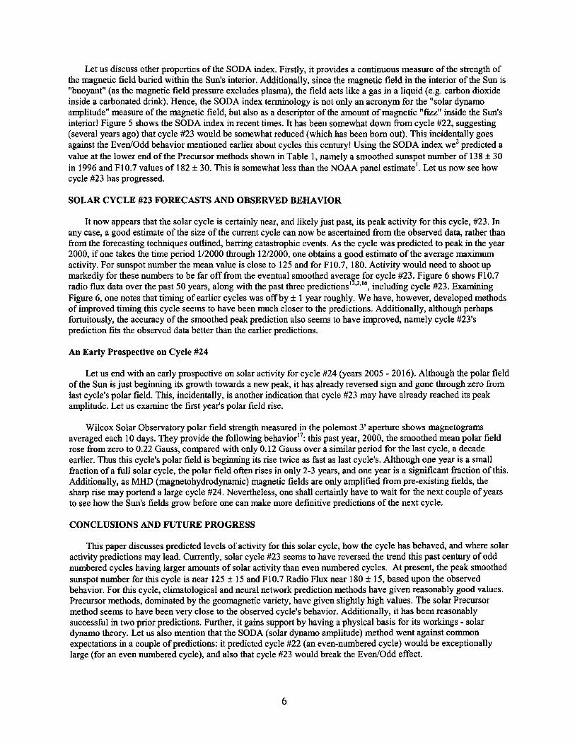
Letusdiscussotherpropertiesof the SODA index. Firstly, it provides a continuous measure of the strength ofthe magnetic field buried within the Sun's interior. Additionally, since the magnetic field in the interior of the Sun is"buoyant" (as the magnetic field pressure excludes plasma), the field acts like a gas in a liquid (e.g. carbon dioxide

inside a carbonated drink). Hence, the SODA index terminology is not only an acronym for the "solar dynamoamplitude" measure of the magnetic field, but also as a descriptor of the amount of magnetic "fizz" inside the Sun's

interior! Figure 5 shows the SODA index in recent times. It has been somewhat down from cycle #22, suggesting(several years ago) that cycle #23 would be somewhat reduced (which has been born out). This incidentally goesagainst the Even/Odd behavior mentioned earlier about cycles this century! Using the SODA index we 2 predicted a

value at the lower end of the Precursor methods shown in Table 1, namely a smoothed sunspot number of 138 + 30

in 1996 and F10.7 values of 182 + 30. This is somewhat less than the NOAA panel estimate 1. Let us now see howcycle #23 has progressed.

SOLAR CYCLE #23 FORECASTS AND OBSERVED BEHAVIOR

It now appears that the solar cycle is certainly near, and likely just past, its peak activity for this cycle, #23. Inany case, a good estimate of the size of the current cycle can now be ascertained from the observed data, rather thanfrom the forecasting techniques outlined, barring catastrophic events. As the cycle was predicted to peak in the year

2000, if one takes the time period 1/2000 through 12/2000, one obtains a good estimate of the average maximumactivity. For sunspot number the mean value is close to 125 and for F10.7, 180. Activity would need to shoot up

markedly for these numbers to be far off from the eventual smoothed average for cycle #23. Figure 6 shows F 10.713216

radio flux data over the past 50 years, along with the past three predictions ' ' , including cycle #23. Examining

Figure 6, one notes that timing of earlier cycles was off by + 1 year roughly. We have, however, developed methods

of improved timing this cycle seems to have been much closer to the predictions. Additionally, although perhapsfortuitously, the accuracy of the smoothed peak prediction also seems to have improved, namely cycle #23's

prediction fits the observed data better than the earlier predictions.

An Early Prospective on Cycle #24

Let us end with an early prospective on solar activity for cycle #24 (years 2005 - 2016). Although the polar fieldof the Sun is just beginning its growth towards a new peak, it has already reversed sign and gone through zero from

last cycle's polar field. This, incidentally, is another indication that cycle #23 may have already reached its peakamplitude. Let us examine the first year's polar field rise.

Wilcox Solar Observatory polar field strength measured in the polemost 3' aperture shows magnetogramsaveraged each 10 days. They provide the following behaviorS7: this past year, 2000, the smoothed mean polar field

rose from zero to 0.22 Gauss, compared with only 0.12 Gauss over a similar period for the last cycle, a decadeearlier. Thus this cycle's polar field is beginning its rise twice as fast as last cycle's. Although one year is a small

fraction of a full solar cycle, the polar field often rises in only 2-3 years, and one year is a significant fraction of this.

Additionally, as MHD (magnetohydrodynamic) magnetic fields are only amplified from pre-existing fields, thesharp rise may portend a large cycle #24. Nevertheless, one shall certainly have to wait for the next couple of yearsto see how the Sun's fields grow before one can make more defmitive predictions of the next cycle.

CONCLUSIONS AND FUTURE PROGRESS

This paper discusses predicted levels of activity for this solar cycle, how the cycle has behaved, and where solar

activity predictions may lead. Currently, solar cycle #23 seems to have reversed the trend this past century of oddnumbered cycles having larger amounts of solar activity than even numbered cycles. At present, the peak smoothed

sunspot number for this cycle is near 125 + 15 and F10.7 Radio Flux near 180 + 15, based upon the observed

behavior. For this cycle, climatological and neural network prediction methods have given reasonably good values.Precursor methods, dominated by the geomagnetic variety, have given slightly high values. The solar Precursor

method seems to have been very close to the observed cycle's behavior. Additionally, it has been reasonablysuccessful in two prior predictions. Further, it gains support by having a physical basis for its workings - solardynamo theory. Let us also mention that the SODA (solar dynamo amplitude) method went against common

expectations in a couple of predictions: it predicted cycle #22 (an even-numbered cycle) would be exceptionallylarge (for an even numbered cycle), and also that cycle #23 would break the Even/Odd effect.

Thus,asfarasthefieldofsolaractivityprediction,thereissomesupportthatjustasintheearlydaysofweatherforecasting,wehavehitsandmisses,butthefieldasawholeismakinggainsbothinunderstandingandimprovementsinforecastingskills.Nevertheless,therearestillareaswherethefieldofsolaractivitypredictionhaslittleorminimalability.Letusatleastmentiontheareaswherethesolarcommunityhaslittleabilityandhencewhereimprovementswouldbehelpful.Evenif embarrassing,discussingtheseareasatleastpointsthewaywhereroomexistsforfutureprogress.

Solaractivityprediction/forecastingislacking,orcouldmakeimprovementsinthefollowingareas:

1. ShortTimeScales- Solar predictions on short time scales, less than decadal, have not been highlysuccessful. For each time scale, one needs to consider the data involved, and must utilize sufficient

observations consistent with the time scale one wishes to predict. Since solar variations occur both on veryshort time scales (days) and moderate time scales (monthly to yearly), there certainly is room for improved

prediction on these time scales. High quality data sources with appropriate physical methods would need tobe employed, considering Sun-Earth geometry, the location of active regions on the Sun's disk, etc.

2. Solar Cycle Timing - Although progress in this area is has been made by utilizing the equatorward march of

active regions as the cycle progresses, a number of solar physicists have pointed out the inadequacies inhow one labels and number solar cycles. Namely, solar physicists do this numbering from solar minimum,

which is an ill-defined quantity, subject to minor fluctuations in a number near zero! This just points out

one of many inadequacies in our methodologies.3. Solar Activity "Size" - By this is meant the indices, levels, strength, or generically "size" of solar activity as

it is quantified. From sunspot number to the present day, commonly used F10.7 radio flux, the field useseither ill-defined indices or indices which only approximately measure what really is needed. Namely, forflight dynamics as an example, one often uses F10.7 Radio Flux, and geomagnetic activity levels to

calculate exospheric densities. The real exospheric densities in which satellites orbit, are affected by upperatmospheric processes and their interaction with solar UV and EUV fluxes, as well as geomagnetic

behavior. Thus if one were to search for improvements in satellite orbital prediction on short time scales,one might find that our overall indices scheme (e.g. F10.7) is inadequate to quantify the solar flux. Thus,one would need better ways to quantify solar activity. Tobiska 19and colleagues are making progress in this

area.

4. Solar Activity "Shape" - This may be folded into time scales. However, one may consider "shape" a

separate topic here. The point is, that even though the curve one uses for predictions may capture"average" behavior reasonably well, one could also use updated solar observations to make shape changes,not just to improve the overall level. For example, just as the SODA index updates the state of buried solar

magnetic flux, one could, in principal, use updated solar field information for details of future activity"shape." If solar magnetism increases on the Sun at a particular latitude, one could ascertain where andwhen this magnetism would be amplified and affect future solar activity levels. Although this may seem atall order, it should be mentioned that there is some basis for this; for the past few cycles I have examined

North vs. South solar activity levels and find some correlation with polar field levels in those hemispheres!

So, even though this is at a global level, it has the hope of being directed more locally in the future.

Thus, the field of solar activity predictions is interesting scientifically and practically, both for the valuableinformation it provides in dynamo physics and for its usefulness to NASA and other agencies interested in solar

activity related phenomena, ranging from power grid spikes, to communication blackouts, to satellite orbital

dynamics.

REFERENCES

. Joselyn, J.A., J.B. Anderson, H. Coffey, K. Harvey, D. Hathaway, G. Heckman, E. Hildner, W. Mende, K.

Schatten, R. Thompson, A.W.P. Thomson, and O.R. White, "Panel achieves consensus prediction of Solar

Cycle 23", EOS, Trans. Amer. Geophys. Union, 78, pp. 205, 211-212, 1997.

2. Schatten, K. H., Myers, D. J., and Sofia, S., "Solar Activity Forecast for Solar Cycle 23", Geophys. Res. Lett., 6,605-608, 1996.

3. McNish, A.G., and J.V. Lincoln, Prediction of Sunspot Numbers, Eos, Trans. Amer. Geophys. Union, 30, p.673, 1949.

4. Holland, R.L. and W.W. Vaughan, Lagrangian Least-Squares Prediction of Solar Flux (F 10.7), J. Geophys.Res., 89, 11-16, 1984.

5. Kerridge, D.J., V. Carlaw, and D. Beamish, "A Review of Methods for Solar and Geomagnetic Activity

Forecasting for Application in Space Missions Planning", BGS Technical Report, WM/89/14C (62 pp.)1989.

6. Hathaway, D. Wilson, R., and Reichmarm, d. Geophys. Res. 104, 22,375-22, 388, 1999.

7. Feyma_n, J., and X.Y. Gu, "Prediction of geomagnetic activity on time scales of one to ten years", Rev.

Geophys.,24, 650, 1986.

8. Ohl, A. I. Soln. Dann. No. 12, 84, 1966.

9. Ohl, A. I. and Ohl, G. I. in R. Donnelly, ed. Solar - Terr. Pred. Proc. Boulder, CO, USA. Vol 2, p 246, 1979.

10. Brown, G. M. and Williams, W. R., "Some Properties of the Day-to-Day Variability of Sq(H)", Planet. Sp. Sci.,

17, 455-469, 1969.

11. Bartels, J., "Discussion of time variations of geomagnetic activity indices Kp and Ap, 1932-1961", Ann.

Geophys., 19, 1, 1963.

12. Thompson, R. J., "A Technique for Predicting the Amplitude of the Solar Cycle", Solar Phys. 148_ 383, 1993.

13. Schatten, K. H., Scherrer, P. H., Svalgaard L., and Wilcox, J. M., "Using Dynamo Theory to Predict the

Sunspot Number During Solar Cycle 21", Geophys. Res. Lett., 5, 411, 1978.

14. Schatten, K. H. and Wilcox, J. M., "Response of the Geomagnetic Activity Index Kp to the Interplanetary

Magnetic Field," J. Geophys. Res., 72, 5185, 1967.

15. Sofia, S., Fox, P., Schatten, K., "Forecast Update for Activity Cycle 23 from a Dynamo-Based Method",

Geophys. Res. Lett., 25, # 22, pp. 4149-4152, 1998.

16. Schatten, K.H., and W.D. Pesnell, "An early solar dynamo prediction: Cycle 23 ~ Cycle 22," Geophys. Res.Lett, 20, 2275-2278, 1993.

17. Wilcox Solar Observatory Polar Field strengths, 3' aperture, 20 nhz low pass filter, 2001.

18. Schatten, K. H. and J. A. Orosz "A Solar Cycle Timing Predictor--The Latitude of Active Regions, "Solar

Physics, 125, 185-189, 1990.

19. Tobiska, W.K, et al., "The SOLAR2000 empirical solar irradiance model and forecast tool," d. Atm. Solar Terr.

Phys., 62, 1233-1250, 2000.

TABLE

TABLE1Forecastingtechniquesandpredictedlevels(insmoothedInternationalSunspotUnits)forsolarcycle#23,basedupontheNOAApanelreportbyJoselyn,etal).ThePrecursorlevelshavebeendividedintotheGeomagneticandSolarPrecursormethods.

PREDICTEDSUNSPOTNUMBERSFORSOLARCYCLE#23

TechniqueEven/Odd Behavior

Spectral

Recent ClimatologyClimatologyNeural Networks

Low End of Range165

135

125

75

Smoothed Max Rz2OO

155

155

115

High End of Range235

185

185

155

110 140 170

Precursor:

Geomagnetic Precursor 140 160 180Solar Precursor 108 138 168

Sunspot Number

o1750 1800 1850 1900 1950 2000

Year

Figure 1. Sunspot Number vs. time for the past few centuries. The figure shows "power" in a wide variety of periodsbeyond the famous 11-year Schwabe periodicity. Additionally, major variations exist both on longer and shortertimescales. Further, amplitudes of the cycles vary by more than 100%, in a rather chaotic manner. Epochs occur,

such as during the "Maunder minimum," when solar activity dropped precipitously to near 0. The numbering on thechart shows the "Even/Odd" effect, where this century odd numbered cycles have always been larger than the

previous even numbered cycle (e.g. cycle #19 > cycle #18).

10

Di_sk Dyn_amok3 Bi

iiiiiiiiiii

iiiiiiiiiiiii

Figure 2. Model of a simple Disk Dynamo is shown. The rotation of a conductor inside a magnetic field generates anelectric field. The electric field drives a current, amplifying the initial magnetic field. The resultant amplifiedmagnetic field is then proportional to the initial magnetic field.

Physical basis for solar andgeomagnetic precursor_e¢hniques

Solar Dynamo

Id) lel If)

Figure 3. In the Babcock dynamo, the Sun's polar fields near solar minimum (a) are wrapped up by differentialrotation (b) to form toroidal fields (c). These fields, later in the cycle, float to the Sun's surface and erupt (d) to formactive regions containing sunspots (e). The breakup of these active region fields regenerate the Sun's polar field witha reverse sign (f), allowing the process to repeat anti-symmetrically.

11

SOLAR DYNAMO

PHOTOSPHERE

BASEOF

ZONE

WEAK POLAR FIELD-FEW SUNSPOTS

STRONG POLAR FiELD--MANY SUNSPOTS

°':BPOLAR

Figure 4. Shown is a simple schematic picture of the Babcock dynamo mechanism for two different cycles: a weak

cycle (left) and a strong cycle (right). The complex picture of the temporal dynamics of a solar cycle is simplified in

this picture so that the polar fields and toroidal fields of each cycle are both displayed.

12

$ODAINDEX

300

250 I

-- -- Btoroidal

.... Bpolar--SODA

x 200g_

E

00

150Z

100

5O

1975 1980 1985 1990 1995 2000 2005

TIME,YEAR

Figure 5. The "SOlar Dynamo Amplitude" or SODA index is a composite index attempting to combine the changing

toroida] and po|oidal fields of the Sun. As these fields vary with time, the combined SODA index allows us to

monitor the "buried magnetic flux" present in the Sun's ever-changing dynamo.

13

F10.7 RADIO FLUX OBSERVED AND PREDICTED

350

3O0

250

X

2oo_o

5o

.... F10.7- obse_ed

--F10.7 - Pred cted

(

I

; IJ:lJ& iI.t_i

, _*_1,*._ I')l

: J..--, ,:_E_,:,1' ;i ,',,:_;4',I,li 4 i j _'--I= I,

o_ t j,, te =

,',.I ,, ;:,_ ;,.i, : ._. _._Ii., I ¢ t,,,c_

,l( : , ,vt ,$ I_ |_tiII i. i i wI' ,. , 1',;._

_ I _., . , _: i; k.,.'J I _ . | a=.

_! ;, .; "_. _:L • _'1' "

., i

o194o 195o 196o 197o 198o 1990 2000 2OlO

YEAR

Figure 6. Shown is F10.7 Radio Flux for the past 50 years, and Schatten et al. predictions for the last 3 cycles,

published in advance. Note that cycle #23, the present cycle, seems to be a better fit to the predicted values, both in

timing and amplitude than previous cycles. Although this may be fortuitous, it may also be a sign that our skill level

is increasing.

14