SOILS, HYDROLOGY AND VEGETATION DISTRIBUTION by

SOILS, HYDROLOGY AND VEGETATION DISTRIBUTION

ON A SALINE LANDSCAPE AT HAILSTONE

NATIONAL WILDLIFE REFUGE

by

Russell Fairchild Smith

A thesis submitted in partial fulfillment of the requirements for the degree

of

Master of Science

in

Land Resources and Environmental Sciences

MONTANA STATE UNIVERSITY Bozeman, Montana

May 2012

© COPYRIGHT

By

Russell Fairchild Smith

2012

All Rights Reserved

ii

APPROVAL

of a thesis submitted by

Russell Fairchild Smith This thesis has been read by each member of the thesis committee and has been found to be satisfactory regarding content, English usage, format, citation, bibliographic style, and consistency and is ready for submission to The Graduate School.

Dr. James Bauder (Co-Chair)

Dr. Catherine Zabinski (Co-Chair)

Approved for the Department of Land Resources and Environmental Sciences

Dr. Tracy Sterling

Approved for The Graduate School

Dr. Carl A. Fox

iii

STATEMENT OF PERMISSION TO USE

In presenting this thesis in partial fulfillment of the requirements for a master’s

degree at Montana State University, I agree that the Library shall make it available to

borrowers under the rules of the Library.

If I have indicated my intention to copyright this thesis by including a copyright

notice page, copying is allowable only for scholarly purposes, consistent with “fair use”

as prescribed in the U.S. Copyright Law. Requests for permission for extended quotation

from or reproduction of this thesis in whole or in parts may be granted only by the

copyright holder.

Russell Fairchild Smith May, 2012

iv

DEDICATION I dedicate this thesis to Terri, River and Brooks for their unwavering love and support. Without their patience and understanding, this work would not have been complete. In addition, this thesis is dedicated to the Apsáalooke people that once hunted on the banks of Hailstone Creek. “The ground on which we stand is sacred ground. It is the blood of our ancestors.” -Chief Plenty Coups

v

ACKNOWLEDGEMENTS

I would like to thank Dr. James Bauder and Dr. Cathy Zabinski for their immense

generosity, guidance and patience during the process of field study and writing. In

addition, I owe a great deal of thanks to Robert Dunn and Laura Smith for introducing me

to this project and for their encouragement and support. Lastly, I thank Karen Nelson and

the US Fish and Wildlife Service for sponsoring this research project and supplying the

background information that formed the foundation of this study.

vi

TABLE OF CONTENTS

1. INTRODUCTION ...........................................................................................................1

Landscape Salinization ....................................................................................................1 Saline Seep ...............................................................................................................2 Environmental Stress in Plants ................................................................................3

Salinity Stress...............................................................................................4 Saturation-Anoxia Stress .............................................................................6

Plants as Indicators of Environmental Condition ....................................................6 Zonation and Environmental Gradient.....................................................................7

Thesis Purpose and Study Objectives .............................................................................8

2. SALINIZATION OF A NORTHERN ROCKY MOUNTAIN WILDLIFE REFUGE ....................................................................................................11

Background ...................................................................................................................11 Study Site ......................................................................................................................11

Climate ...................................................................................................................11 Geology ..................................................................................................................13 Soils........................................................................................................................13 Hydrology ..............................................................................................................14 Saline Seep at Hailstone.........................................................................................14

Study Methods ...............................................................................................................16 Vegetation ..............................................................................................................19 Hydrology ..............................................................................................................20 Soils........................................................................................................................21 Data Compilation and Statistical Analysis ............................................................23

3. VEGETATION CHARACTERISTICS OF A SALINE LAKESHORE ENVIRONMENT ..........................................................................................................26

Results ...........................................................................................................................26

Vegetation Band A .................................................................................................26 Vegetation Band B .................................................................................................28 Vegetation Band C .................................................................................................29 Vegetation Band D .................................................................................................30 Plant Diversity .......................................................................................................31 Wetland Indicator Status by Position .....................................................................33 Common Species within Bands .............................................................................34

Salicornia ...................................................................................................34 Suaeda calceoliformis ................................................................................36 Distichlis spicata ........................................................................................37 Poa pratensis .............................................................................................38

vii

TABLE OF CONTENTS – CONTINUED

Vegetation and Position .........................................................................................38

Conclusions ...................................................................................................................38

4. ABIOTIC CONDITIONS OF A SALINE LAKESHORE ENVIRONMENT..............41

Results ...........................................................................................................................42

Landscape Characteristics ......................................................................................42

Hydrology ..............................................................................................................42

Position A...................................................................................................45

Position B ...................................................................................................45

Position C ...................................................................................................45

Position D...................................................................................................45

Soils........................................................................................................................46

Position A...................................................................................................46

Position B ...................................................................................................47

Position C ...................................................................................................49

Position D...................................................................................................49

Position, Saturation, and Salinity ...........................................................................50

Nutrients .................................................................................................................52

Conclusions ...................................................................................................................55

5. DISCUSSION ................................................................................................................56

Synopsis.........................................................................................................................56

Synthesis ................................................................................................................57

Biotic Factors .............................................................................................60

Applications ...........................................................................................................60

Revegetation Zone 1 ..................................................................................65



Conclusions ...................................................................................................................71

REFERENCES ..................................................................................................................74

APPENDICES ...................................................................................................................81

APPENDIX A: Vegetation Percent Cover ...................................................................82

APPENDIX B: Tables of Statistical Analysis ..............................................................84

viii

LIST OF TABLES

Table Page

1. Landscape characteristics .................................................................................. 19

2. U.S. USFWS Wetland Indicator Categories ..................................................... 20

3. Passive hydrologic indicators. .......................................................................... 21

4. Soil chemistry parameters analyzed.................................................................. 22

5. Salt affected soils classification ........................................................................ 25

6. Vegetation at Hailstone organized by family.................................................... 27

7. Band A vegetation summary ............................................................................. 28

8. Band B vegetation summary ............................................................................. 29

9. Band C vegetation summary ............................................................................. 30

10. Band D vegetation summary ........................................................................... 31

11. Two diversity indices with richness, by vegetation band position. ................ 33

12. Vegetation type and mean percent coverage summary by band. .................... 34

13. Prioritization of most common species for within-position analysis .............. 35

14. Length, height differential from point A to D ................................................. 43

15. Mean sample points distance from water surface ........................................... 43

16. Mean depth to saturation ................................................................................. 44

17. Soil Summary – Position A............................................................................. 47

18. Soil Summary – Position B ............................................................................. 48

19. Soil Summary – Position C ............................................................................. 49

ix

LIST OF TABLES - CONTINUED

Table Page

20. Soil Summary – Position D............................................................................. 50

21. Average depth weighted N, nitrate-N, and ammonium .................................. 52

22. Average depth weighted total P (Bray-1) and orthophosphate ....................... 53

23. Average depth weighted potassium and sodium concentrations .................... 54

24. Hailstone salinity/saturation conditions by revegetation zone........................ 65

25. Hailstone vegetation guide by zone. ............................................................... 65

x

LIST OF FIGURES

Figure Page

1. The process of saline seep on a landscape .......................................................... 3

2. Environmental conditions examined................................................................... 9

3. Location Map of Hailstone National Wildlife Refuge ...................................... 12

4. 1941 Aerial Photograph of Hailstone Lake ...................................................... 15

5. Sample point locations ...................................................................................... 17

6. An example of vegetative banding ................................................................... 18

7. Transect 105 ...................................................................................................... 18

8. Percent bare ground by position ....................................................................... 32

9. Inverse Simpson’s and Shannon Wiener diversity indices. .............................. 33

10. Percent canopy cover across A-D positions.................................................... 40

11. Position vs. sample point elevation and depth to saturation ........................... 44

12. Percent OM vs. position by depth. .................................................................. 47

13. Periodic soil-saturation ................................................................................... 48

14. Averaged depth-weighted EC ......................................................................... 51

15. EC depth profile by position ........................................................................... 51

16. Conceptual model ........................................................................................... 57

17. Scatter plot of depth weighted EC .................................................................. 62

18. Mean depth weighted EC for short transects vs. long transects ..................... 62

19. Revegetation profile for three zones. .............................................................. 68

xi

LIST OF FIGURES - CONTINUED

Figure Page

20. A conceptual map of revegetation zones ........................................................ 69

21. Example of vegetated islands and banding ..................................................... 71

xii

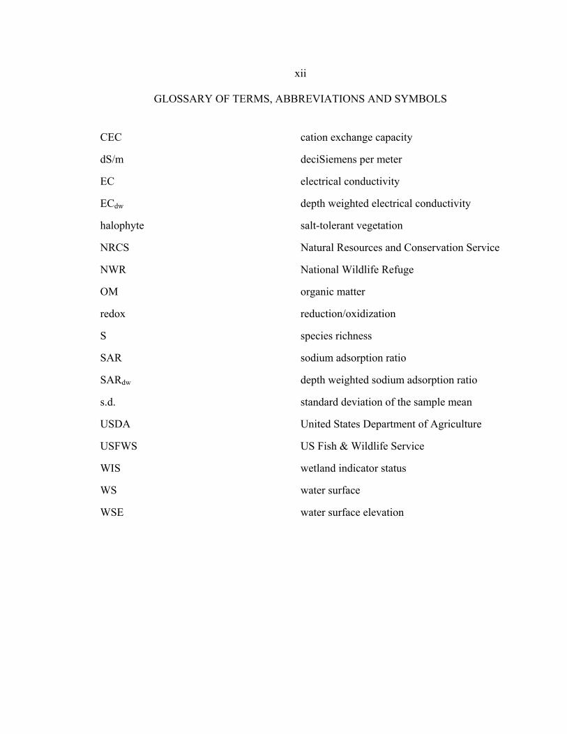
GLOSSARY OF TERMS, ABBREVIATIONS AND SYMBOLS

CEC cation exchange capacity

dS/m deciSiemens per meter

EC electrical conductivity

ECdw depth weighted electrical conductivity

halophyte salt-tolerant vegetation

NRCS Natural Resources and Conservation Service

NWR National Wildlife Refuge

OM organic matter

redox reduction/oxidization

S species richness

SAR sodium adsorption ratio

SARdw depth weighted sodium adsorption ratio

s.d. standard deviation of the sample mean

USDA United States Department of Agriculture

USFWS US Fish & Wildlife Service

WIS wetland indicator status

WS water surface

WSE water surface elevation

xiii

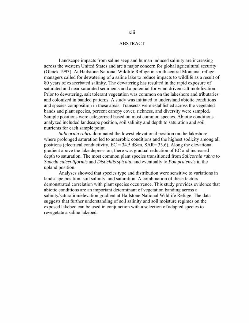
ABSTRACT

Landscape impacts from saline seep and human induced salinity are increasing across the western United States and are a major concern for global agricultural security (Gleick 1993). At Hailstone National Wildlife Refuge in south central Montana, refuge managers called for dewatering of a saline lake to reduce impacts to wildlife as a result of 80 years of exacerbated salinity. The dewatering has resulted in the rapid exposure of saturated and near-saturated sediments and a potential for wind driven salt mobilization. Prior to dewatering, salt tolerant vegetation was common on the lakeshore and tributaries and colonized in banded patterns. A study was initiated to understand abiotic conditions and species composition in these areas. Transects were established across the vegetated bands and plant species, percent canopy cover, richness, and diversity were sampled. Sample positions were categorized based on most common species. Abiotic conditions analyzed included landscape position, soil salinity and depth to saturation and soil nutrients for each sample point. Salicornia rubra dominated the lowest elevational position on the lakeshore, where prolonged saturation led to anaerobic conditions and the highest sodicity among all positions (electrical conductivity, EC = 34.5 dS/m, SAR= 33.6). Along the elevational gradient above the lake depression, there was gradual reduction of EC and increased depth to saturation. The most common plant species transitioned from Salicornia rubra to Suaeda calceoliformis and Distichlis spicata, and eventually to Poa pratensis in the upland position. Analyses showed that species type and distribution were sensitive to variations in landscape position, soil salinity, and saturation. A combination of these factors demonstrated correlation with plant species occurrence. This study provides evidence that abiotic conditions are an important determinant of vegetation banding across a salinity/saturation/elevation gradient at Hailstone National Wildlife Refuge. The data suggests that further understanding of soil salinity and soil moisture regimes on the exposed lakebed can be used in conjunction with a selection of adapted species to revegetate a saline lakebed.

1

INTRODUCTION

Landscape Salinization

Across the globe, soil salinization has become an important landscape degradation

problem. Primary minerals in exposed layers of the earth’s crust are the main source of

salts and these constituents are mobilized by the process of chemical weathering via

hydrolysis, hydration, solution, oxidization, and carbonation (Sandoval and Gould 1978).

Naturally occurring salinity on the surface of the landscape prior to modern agricultural

practices has been well documented. According to oral history, the Apsáalooke people

who migrated throughout the northern and southern plains of North America, “came upon

lakes with salt on their banks” (Crow 2012). During their travels across the northern

Great Plains in the early 19th Century, Lewis and Clark documented many areas where

the white crusts of surface salts occurred on the landscape. In these areas, soils contained

sufficient salts on the surface to negatively affect the growth of most plants, as William

Clark noted in his journals.

“…[T]he granulated salt is found on the surface of a compact and hard earth composed of fine sand with a small proportion of clay producing no vegitable [sic] substance of any kind.” (Lewis et al. 2002). Three factors contribute to depressing plant growth on saline landscapes: 1) salts

prevent plant roots from soil water uptake as a result of increased osmotic tension, 2)

chemical effects of salts disrupt nutritional and metabolic function in plants, and 3) salts

alter soil structure by changing permeability for air and water (Thorne and Peterson

2

1949). These environmental conditions occur as a result of unique geologic and

hydrologic conditions and certain land use practices such as alternate crop fallow can

exacerbate salinization of soils and affect water quality.

Saline Seep

During the early 20th century, native grasslands in the Northern Plains were

plowed for agricultural production (Holzer et al. 1995). After the 1950’s, more efficient

farming equipment was used to plow larger areas of native sod while at the same time,

widespread initiation of alternative crop-fallow farming systems in the Northern Plains

began. The practice of crop-fallow increases soil moisture for subsequent use by crops in

the following growing season, and like a plowed field, can increase the rate and amount

of water infiltration past the rooting zone. The process of saline seep is initiated when

excess moisture leaves the rooting zone and migrates downward. When water encounters

soil discontinuity, such as bedrock or clay (aquatard), it moves laterally, solubilizing and

mobilizing salts as it travels to a discharge area on the soil surface, creating a seep

(Figure 1). As the water evaporates on the ground surface, the salts are left behind. In

times of increased rainfall, salinity problems can be more severe due to greater recharge

and therefore accumulation of salt-laden water in the recharge zone (Abrol et al. 1988).

By 1983 it was estimated that over 800,000 hectares of agricultural production in the

United States and Canada had been affected by saline seep (Nelson and Reiten 2009).

3

Figure 1. The process of saline seep on a landscape begins with excessive moisture moving past the rooting zone (top left), downward and laterally across a less permeable layer, mobilizing solutes as the water moves down-gradient. If the water interacts with the surface, the solutes are deposited on the soil through evapoconcentration (bottom right) and a seep results. (Figure courtesy of MSU Extension Services, Soil & Water Management Module No. 2. McCauley and Jones 2005.)

Typically, landscapes associated with seep maintain a soil salinity gradient, or a

transition from high to low salt concentration in an outward direction, away from the

source of water contributing to the seep. Plant species tend to follow these gradients

based on their respective toleration to the environmental stress. With advances in seep

reclamation over the last two decades, researchers came to the conclusion that salinized

soils could be stabilized and their detrimental effects on the landscape could be alleviated

by planting halophytes (salt tolerant plants) as well as altering hydrologic regimes

(Holzer et al. 1995; Sanderson et al. 2008). Understanding the effect of stress on

vegetation is crucial in reclamation of saline seep.

Environmental Stress in Plants

At the plant level, stress can be defined as “any external factor that negatively

influences plant growth, productivity, reproductive capacity or survival” (Rhodes and

LESS PERMEABLE LAYER

4

Nadolska-Orczyk 2001). This includes a wide range of causes, which can be generally

separated into two main groups: environmental stress factors (abiotic) and biological

stress factors (biotic). At the community level, researchers have posited that

environmental stress (both abiotic and biotic) is a primary driver of species composition.

Bertness and Callaway (1994) proposed a conceptual model that predicted higher

frequency of positive interaction (facilitation) between species at high abiotic stress

where tolerant species promote subsequent growth for other species. Concurrently, the

frequency of competition is higher at low abiotic stress as a result of the ability of more

species to tolerate lower stress levels. Two primary stress factors affecting plant growth

at Hailstone are salinity stress and anoxia/saturation stress.

Salinity Stress. Plants vary in their degree of salt tolerance and in the means by

which they regulate salt content in their tissues. Most plants are salt sensitive

(glycophytes), and these species show little tolerance to elevated root-zone salinity.

Excessive salts in the soil (low osmotic potential) limits the uptake of water by plants,

and may result in the lowering of tissue turgor, resulting in wilting (Zhu 2001). Many of

these naturally occurring saline lands maintain plant communities that have, through

evolutionary processes, adapted to these conditions. Halophytes are ecologically,

physiologically and biochemically specialized plants, capable of producing green mass

and seeds while growing in a saline substrate (Wickens 1989; Shamsutdinov and

Shamsutdinov 2009), but most halophytes exhibit decreased growth at extremely high

salt concentrations (Nilsen et al. 1996; Glenn et al. 1999; Barrett-Lennard 2002; Tester

and Davenport 2003). In addition, salt tolerant plants of arid regions have also become

5

adapted to harsh xerothermic effects, such as extreme air and soil dryness, as well as high

summer and low winter temperatures (Shevyakova et al. 2003).

Halophytes respond to saline environments through tolerance, which is the

capability to preserve normal metabolic activity even in the presence of high intracellular

salt levels (salt accumulators); and avoidance, where the plants do not allow the

penetration of salt ions into their cells (Manousaki and Kalogerakios 2011). Plants utilize

avoidance mechanisms in three ways: 1) exclusion through low permeability to salts, 2)

excretion of some penetrating ions, and 3) isolation through ion retention (Mozafar and

Goodin 1970; Flowers et al. 1977; Ramadan 1998; Glenn et al. 1999). Glycophytes

maintain similar function but at lower rates, and are not as effective in reducing salt stress

(Nilsen et al. 1996; Nelson et al. 1998).

Plants require macronutrients and micronutrients in various forms for normal

functioning and growth as well as to deal with increasing stress. Nutrient levels outside of

the optimum level for sufficient plant growth will cause overall health and growth to

decline due to either a deficiency or toxicity (Jones and Jacobsen 2005a). Sodium is a

functional nutrient for many plants (Subbarao et. al. 2003) but because of its ubiquitous

presence in soils, it is rarely considered limiting. Plants utilize three biochemical

mechanisms for fixing carbon in tissue growth: C3, C4 and CAM photosynthesis. While

C3 and C4 plants are named for their carbon molecules present in the first product of

carbon fixation, CAM (Crassulacean acid metabolism) is an adaptation for increased

efficiency in the use of water and is typically found in plants growing in arid

environments (Herrera 2008). In C4 plants, sodium (Na+) is a micronutrient that aids in

6

metabolism and synthesis of chlorophyll (Kering 2008) and in some species it substitutes

for potassium in several roles, such as maintaining turgor pressure and aiding in the

opening and closing of stomata (Subbarao et al. 2003). Nevertheless, beyond optimal

levels, sodium and salts negatively affect plant growth. In addition to stress induced by

salinity, plants also face stress from lack of oxygen in saturated soils.

Saturation-Anoxia Stress. Plant growth is dictated in part by oxygen availability

in the soil, as roots require oxygen for cellular respiration, which fuels virtually all

metabolic processes in plants. Under aerobic conditions, plants produce up to 19 times

more ATP molecules than plants under anaerobic conditions (Barrett-Lennard 2002).

Wetland plants have developed physiological adaptations to anoxic conditions to increase

oxygen access to the roots. These include 1) aerenchyma: hollow root channels, 2)

adventitious roots: that which grows from an unusual location such as the base of a tree to

avoid soil saturation/anoxia, and 3) hypertrophy: e.g. enlarged lenticels where cell

aggregation creates a channel on the stem surface which allows for gas exchange. Plants

species’ distribution varies across moisture gradients because of species’ varying degrees

of tolerance to the effects of saturated soil and because of plants’ varying tolerances to

lack of moisture.

Plants as Indicators of Environmental Condition

The presence of a plant species at an individual location will depend on a variety

of edaphic, biotic, and climatic factors as well as the effect of individual factors, such as

depth and duration of soil saturation or inundation (Cowardin 1978). In 1988, The U.S.

7

Fish and Wildlife Service (USFWS) in cooperation with a federal inter-agency review

panel developed a national list of plant species that occur in wetlands (Reed 1988;

USFWS 1988). This inventory was compiled as a list of over 7,000 plants in 13 separate

regions of the United States. A plant’s wetland indicator status (WIS) is applied to the

species as a whole within each USFWS region where differences exist with ecotypic

variation (Tiner 1991). This classification scheme has found widespread use as a general

reference tool for grouping plants based on their known tolerance to saturation/anoxia.

Utilizing known indices for associating species with tolerance to saturation (or salinity)

can form the basis of comparing vegetation characteristics to the formation of zones

based on environmental condition.

Zonation and Environmental Gradient

Zonation is defined as the formation of distinct features, common physical

characteristics or components, (Biology Online 2012) and is a patent growth

characteristic of vegetation in many wetlands (Stewart and Kantrud 1971; Snow and

Vince 1984; Mitsch and Gosselink 2007). Wetland plant species tend to occupy a

characteristic vertical range in relation to a water body, and species assemblages often

appear as bands on the landscape. Environmental conditions within each band may

represent optimal habitat for resident plant species (Snow and Vince 1984). Sanderson et

al. (2008) described how abiotic environmental gradients governed vegetation zonation in

an intermountain playa and found through reciprocal transplant experiments that plant

species produced maximum biomass in their native zone and plant zonation appeared

particularly strong on the most stressful ends of the abiotic gradient. Horsnell et al.

8

(2009) described the importance of temporal hydroperiod thresholds on the growth of

various halophytes, mesophytes, phreatophytes, and xerophytes at a site in Western

Australia, and in order to understand sensitivity to waterlogging and salinity, the authors

established a ‘coping’ range for plants targeted for conservation.

Waterlogging and salinity at the soil surface are important factors that regulate

plant growth and establishment. McFarlane and Williamson (2002) found that water-

logging may be more of an inhibitor to plant growth than salt even at high salt levels. The

interaction of salt and water is synergistic for plants; some plants utilize additional water

to offset the negative effects of increased salinity via osmoregulation and other adaptive

mechanisms (Hasegawa et al. 2000). Studies have also suggested that plants compete

more in less stressful conditions and poorer competitors are displaced to more stressful

habitats, and that both biotic and abiotic factors play a role in plant species zonation

(Bertness and Ellison 1987; Keddy 1989; Rand 2000; Costa et al. 2003).

Thesis Purpose and Study Objectives

The primary objective of this study was to examine patterns of plant assemblages

on a saline lake shoreline and to elucidate the abiotic characteristics occurring in

association with them. Although biotic factors (i.e. facilitation, competition, etc.) likely

played a role in the pattern of vegetation growth at the site, the purpose of this study was

to understand the abiotic processes to support future approaches for revegetation of

exposed saline soils where little or no vegetation grows.

9

The study was conducted in the summer of 2010 along the shoreline of Hailstone

Lake, the primary landscape feature on a National Wildlife Refuge in south-central

Montana. I examined plant species composition, percent ground cover and diversity;

landscape position, soil saturation and salinity. Figure 2 depicts the environmental

characteristics that were examined and served to guide the approach of the observational

study.

Figure 2. Environmental conditions examined in a study of plant growth characteristics at Hailstone National Wildlife Refuge.

The objectives for the study were as follows:

1) Vegetation. Identify vegetation on selected sampling points, measure canopy

cover by species, determine species richness and calculate diversity. Classify

plants using known indices for anoxia/saturation and saline tolerance.

Vegetation

Species Type

% Canopy Cover

Species Richness

Species Diversity

Landscape

Transect Length

Point Elevation

Point Distance to WS

Hydrology

Pit Depth to

Saturation

Pit Depth to Free Water

Soils

Texture

Electrical Conductivity

OM

Nutrients

10

2) Landscape. Measure physical characteristics of transects and sampling points

including transect length, point elevation from water surface and point distance

from water surface.

3) Hydrology. Measure soil depth to saturation and passive indications of

hydrologic influence such as drifted organic matter and oxidized root channels.

4) Soils. Measure soil chemistry (nutrients, pH, EC), texture-by-feel and visual

indications of reduction/oxidation.

5) Association. Identify significant associations between abiotic conditions and

vegetation characteristics.

6) Recommendations. Using collected data and interpretation of associations,

provide land managers with recommendations for revegetation.

In the arid Rocky Mountain west, there are increasing pressures on fresh water

resources from agriculture, urban development and from potential modification of

regional hydrology with changing global climate dynamics. Given these pressures,

solutions are needed to address the adverse impacts of salinization and apply knowledge

of vegetation response to abiotic factors that affect spatial distributions of vegetation.

This thesis will contribute to our understanding of vegetation spatial patterns in inland

saline environments.

11

SALINIZATION OF A NORTHERN ROCKY MOUNTAIN

WILDLIFE REFUGE

Background

This study was conducted in response to high salinity conditions at Hailstone

National Wildlife Refuge in northern Stillwater County (Figure 3), 46° 00’ 24” N, 109°

10’ 50” W, south-central Montana. Hailstone was characterized as one of the ten most

endangered wildlife refuges in the USFWS refuge system (Schlyer 2007) and in 2009, the

USFWS identified the primary management challenges as waterfowl and shorebird

mortality due to high salt concentrations. Elevated selenium was also a contributing

factor to wildlife mortality (although not examined in this study) and these solutes were

concentrated in Hailstone reservoir, the primary aquatic feature and waterfowl attractant

on the refuge. In addition, blowing salt dust from exposed lakeshore and saline seeps

proved to be a nuisance to adjacent landowners and land managers (Nelson and Reiten

2009), and solutions to stabilize exposed soils at the refuge were initiated.

Study Site

Climate

Hailstone and Lake Basin have a semiarid climate with cold winters and hot

summers. The local region is at the convergence of the Great Basin and Rocky

Mountains, and is climatically influenced by both (Nelson and Reiten 2009). Average

precipitation, based on Western Regional Climate Center records, is approximately 33

cm, 43 percent of which falls during April through June (WRCC 2011). Average air

12

Figure 3. Location Map of Hailstone National Wildlife Refuge, Northern Stillwater County, MT. From USGS-SDSS 2012.

Hailstone Lake

13

temperature for the region is 9.1 °C with an average maximum of 15.4 °C and a

minimum of 2.8 °C. The 30-year average growing degree days for calendar dates March

1st through November 26nd for the nearby community of Rapelje, MT, is 1,810 (NOAA

2011).

Geology

Hailstone Basin is located near the crest of the Big Coulee-Hailstone structural

dome and is found on the northern fringe of the Lake Basin (Lopez 2000). The northern

Hailstone Basin is made of Eagle Sandstone and the southern boundary lies on a fault

zone made of steeply dipping rock of the Cretaceous Montana Group. The subsurface of

the basin is made up of marine shale, primarily the Niobrara formation and are the source

of salts at Hailstone (Nelson and Reiten 2009). This layer acts as a barrier to movement

of groundwater (aquatard) and is one cause of exacerbated salinization within the basin.

A narrow breach in the fault zone once allowed (albeit infrequently) surface drainage to

flow out of Hailstone Basin into the internally drained Lake Basin (Nelson and Reiten

2009).

Soils

Soils along the lakeshore vary from Lardell clay loam, to Absher clay loam

(USDA, NRCS 2012) and though soil survey mapping data are known to omit small-

scale soil units (inclusions), they are largely representative of the area.

14

Hydrology

The watershed basin is approximately 12,633 hectares in size and prior to refuge

establishment, an earthen dam was constructed across Hailstone Creek in 1938 as a

Works Progress Administration project (Nelson and Reiten 2009), resulting in the

formation of Hailstone Lake. The 1,112-hectare wildlife refuge was created in 1942 as a

breeding ground for waterfowl and shorebirds. The lake initially inundated a small

oxbow of Hailstone Creek and backwater wetland (Figure 4) approximately 65 hectares

in area, but by 1979 expanded to a salty playa of nearly 259 hectares. Hailstone Lake was

approximately 226 hectares but rarely did it get high enough to allow water to exit the

concrete spillway. Almost all losses were through evaporation, which was the primary

cause of elevated salt concentrations in the lake.

Prior to the commencement of dewatering in 2010-11, groundwater flow in the

basin moved generally from the edges toward the reservoir and was perched on Niobrara

shale (Nelson and Reiten 2009). Recharge potential was greater at the higher

permeability margins where loose colluvial sediments from adjacent hill slopes fell, and

decreased toward the center of the basin where denser alluvial sediments accumulated. A

majority of the earthen embankment and the entire concrete spillway was removed in the

summer of 2011, and historic flow regimes were restored to the lower channel.

Saline Seep at Hailstone

In 1974 the Montana Department of State Lands ranked Stillwater County as

having the most saline-affected dryland acres in the state at approximately 9,300 hectares

15

Figure 4. 1941 Aerial Photograph of Hailstone Lake, three years after the earthen dam was constructed on the perennial channel (highlighted in red). Note surface salinity in white at the top of photo. Photo courtesy of Nelson and Reiten 2009.

(Kellogg 1984), and it was estimated in 1980 that saline seeps were increasing at a rate of

10 percent annually (Miller et al. 1980). Inspection of aerial photographs revealed that

Hailstone Basin experienced wide development of saline seep since dam construction and

crop-fallow farming practices were initiated in the late 1940’s. The saline seeps

developed in groundwater transitions zones where a slight rise in bedrock forced water

toward the land surface (Nelson and Reiten 2009).

Dominant soluble salts found in the soils at Hailstone are sodium, magnesium,

calcium chloride, sulfates and bicarbonates. Water moving from the recharge area (as a

result of precipitation infiltration) to the discharge area (seep) accumulates approximately

50 mg/L of total dissolved solids (TDS) per foot of movement, depending on rate of

16

groundwater flow and concentrations of available salts (Nelson and Reiten 2009). A lack

of sufficient seasonal flushing resulted in further concentration and accumulation of salts.

Miller et al. (1980) calculated that there may be enough sodium in the shallow aquifer to

sustain seeps from 25 to 100+ years.

Study Methods

Vegetation, landscape position, soils and hydrology on the shoreline of Hailstone

Lake were the focus of this study. In 2010, ten transects were established along the

transition from the shore of the lake and tributaries to adjacent native upland prairie

(Figure 5). It was postulated that environmental characteristics would change with the

dewatering of the lake, so the study was initiated as a ‘point-in-time’.

Transect locations were chosen based on the presence of vegetation bands with

visually distinct dominant species. These distinct vegetation assemblages generally

paralleled the shoreline and appeared to represent a transition, progressing from wetland

to an upland environment (Figure 6). Transects were oriented perpendicularly from the

shore (or tributary swale) and across the bands of vegetation. Along each of the 10

transects, 1 sample point was randomly located within each of the 4 vegetation

assemblages (n=40). Sample points were labeled A through D; ‘A’ being closest to the

lake (or swale) and ‘D’ furthest away into the upland position (Figure 7). Landscape

characteristics (Table 1) were measured at the 40 sample points.

17

Figure 5. Sample point locations (black circles) at Hailstone National Wildlife Refuge. From USGS-SDSS 2012. Note: Lake level depicted in this map was not reflective of conditions at time of sampling. All transects and sample points were on or outside the margins of the lake.

18

Figure 6. An example of vegetative banding on the western shore of Hailstone Lake in March 2010.

Figure 7. Transect 105 and approximate sample point locations in July 2010 oriented across a dry inflow channel to the northwest of the impoundment. Sample points were codified to reflect their relative position on the landscape; A (channel bottom) through D (upland).

D C AB

A

B

CD

19

A benchmark was created at each transect origin, representing approximately the

closest point of the lake at the time of measurement, or, in the case of tributary transects,

the bottom of the channel. (At the time of sampling, July 7 to August 3, 2010, tributaries

were not flowing.)

Table 1. Landscape characteristics that were measured for each transect and at sample points.

Physical Parameter Units

GPS location lat / long

Elevation from water surface meters

Point distance from water surface meters

Transect length from A - D meters

Transect aspect northing

General location (lakeshore, tributary) as applicable

Vegetation

A 50 cm x 50 cm vegetation sampling frame was randomly placed within each

dominant band of vegetation and all plants occurring within the sampling frame were

identified to species using Dorn (1984), Flora of North America (1993), and Weeds of the

West (Whitson 1991). The Plants Database (USDA, NRCS 2012) was used for final

taxonomic nomenclature. Percent foliar cover (percentage of ground covered by aerial

portions of the plants) of each species was also estimated and recorded.

Species were categorized using USFWS Wetland Indicator Status (Table 2) for

the North Plains Region 4 (Eastern Montana). These indicators reflect the range of

estimated probabilities of a species occurring in wetlands versus non-wetlands across the

entire known distribution of the species. This classification scheme is not indicative of

moisture status throughout the growing season, but rather an indication that sufficient

20

moisture is available for maintenance of vegetation during the growing season. These

classes are intentionally broad and can represent a range of intra- and interspecific

moisture tolerances (USFWS 1988). For this study, they were useful in grouping

sampling points based on moisture affinity and were not intended to be used as indicators

of species abundance.

Hydrology

Indication(s) of active hydrology (free-water and/or saturation) was examined at

each sampling point. In addition to visual observations of conditions on the soil surface,

primary observation pits were dug to 60 cm with a shovel and left open for approximately

20 minutes at each sampling point to allow for groundwater seepage (as free-water,

where present) to flow into the pits.

Table 2. U.S. USFWS Wetland Indicator Categories used in this observational study. From USFWS Biological Report 88 [26.9] 1988, Revised 1993.

Indicator Code

Wetland Type

Comment

OBL Obligate Wetland

Occurs almost always (estimated probability 99%) under natural conditions in wetlands.

FACW Facultative Wetland

Usually occurs in wetlands (estimated probability 67%-99%), but occasionally found in non-wetlands.

FAC Facultative Equally likely to occur in wetlands or non-wetlands (estimated probability 34%-66%).

FACU Facultative Upland

Usually occurs in non-wetlands (estimated probability 67%-99%), but occasionally found on wetlands (estimated probability 1%-33%).

UPL Obligate Upland

Occurs in wetlands in another region, but occurs almost always (estimated probability 99%) under natural conditions in non-wetlands in the regions specified. If a species does not occur in wetlands in any region, it is not on the National List.

NI No indicator Insufficient information was available to determine an indicator status.

21

In pits having no free-water, saturation depth was measured to the presence

glistening soils on the pit walls. This latter condition indicated that water was either

actively draining downward or wicking upward at some point between field capacity and

saturation. Many factors can affect a soil under this condition but in this study, this

assumption was meant to serve as a practical measure of soil water having influence on

vegetation at the sample pit. In addition, Table 3 describes passive indications of

hydrology, and served to support evidence of hydrologic influence at sample points if

seasonal hydrology had ceased or was transitory in nature.

Table 3. Passive hydrologic indicators.

Passive Hydrologic Indicators

High-water Marks

OM Drift Lines

Drainage Patterns

Oxidized Root Channel

Water-stained Leaves

Soils

At each sampling point, soil samples were taken from a primary pit

(approximately 20 cm in diameter) and two smaller pits (for the purpose of composite

sampling), all of which were dug approximately within the 0.5 m sample frame location.

Soils from all three pits were collected in increments of 0-2 cm (surface), 2-5 cm, 5-10

cm and 10-20 cm, composited in a sealed plastic bag by depth increment, labeled and

placed in a cooler. Depth increments were chosen based on the influence that nutrients,

salinity and saturation have on plant seed germination (0-2 cm), seedling growth (2-5 cm)

22

and mature plant establishment (5-20 cm) during various growth stages. Soils were

returned to the laboratory, thoroughly mixed, placed in a soil bag, dried at 43 °C ± 2 °C

for no less than one week, shipped to Ag Source Harris (Omaha, NE) and analyzed for

soil chemistry. Table 4 lists the parameters and unit value for each parameter.

Table 4. Soil chemistry parameters analyzed.

Soil chemistry parameter

Units

Organic Matter % of dry soil

N mg/kg dry soil

P - Bray 1 mg/kg dry soil

K mg/kg dry soil

pH - log H+ in solution

Na mg/kg dry soil

CEC meq H+/100g

EC dS/m

Na meq/l

Ca meq/l

Mg meq/l

NH4 mg/kg dry soil

NO3 mg/kg dry soil

PO4 mg/kg dry soil

SAR – Sodium Adsorption Ratio

[Na+] / [(Mg2+ + Ca2+)/2]0.5

where cation concentrations are in meq/l – Unitless ratio

At each sampling point, the sample core from the primary pit was inspected for

the presence or absence of redoximorphic soil characteristics using the USDA Field

Indicators of Hydric Soils (USDA, NRCS 2010). This observation was used to compare

hydromorphic condition, i.e., physical evidence of inundation and saturation, with plant

type and landscape position. In addition, soil texture (Thien 1979) was observed for each

soil sample and recorded.

23

Data Compilation and Statistical Analysis

Ten transects had 4 sample points for each position A – D, which served as

replications. Vegetation, landscape, soils, and hydrologic data was compiled using

Microsoft Excel®, and basic statistical analysis was done using the IBM© SPSS©

Statistics 19 environment. One-way analysis of variance (ANOVA) was used in

comparing means among position for the following soil parameters: percent organic

matter (OM), pH, CEC, EC and SAR by position (A, B, C, D). One-way ANOVA was

used in comparing pH, CEC, EC and SAR by depth within each position. Data on percent

OM by position and SAR by depth (position A) failed Levene’s test of equality of error

variance so ANOVA was not calculated. Least square difference tests were used for post

hoc comparisons of within group means. Statistical significance was determined using p-

values at 0.05 or less. Correlations were calculated using Pearson’s test. Sigma Plot® 10

was also used for graphing box plots, which show mean and first quartile, and the

whiskers designate the extreme ends of the variable range (set to extend to 1.5 times the

length of the interquartile range). Points located outside the range of the whiskers (dots

and stars) were considered to be outliers.

To measure plant diversity, Simpson’s (Equation 1) and Shannon-Wiener

(Equation 2) indices were calculated for vegetation samples. A vegetation assemblage

containing only one species would have a Simpson’s value of 1.0; therefore the inverse

was used to show greater values representing higher diversity.

24

Equation 1. Simpson's Diversity Index

1

Where: n = the total proportion (as percent cover or number of individuals) of a particular species

= species richness

Equation 2. Shannon-Wiener Diversity Index.

ln

Where: = proportion of organisms (as percent cover) of a particular species relative to the total number of species.

= species richness

Subscripts are used in reporting and denote soil depth in centimeters or indicate

that a depth weighting transformation was performed (e.g. ECdw) on some soil chemical

parameters. Depth weighing is used to simplify sample point values in some analyses and

is calculated by multiplying the soil depth increment by the parameter value and dividing

the sum of all incremental values by the total sample depth (20 cm).

Equation 3. Depth weighting formula for a 20 cm deep soil sample.

∑ ν

Where: ν parameter value

25

depth increment (cm)

depth total (cm)

Sodium adsorption ratio (SAR) measures the relationship between three dominant

cations; sodium (Na+) to magnesium (Mg2+) and calcium (Ca2+) and is useful in

determining the proportion of sodium in a soil sample (Equation 4). SAR is calculated as

follows and is reported as a unitless measure:

Equation 4. Calculating sodium adsorption ratio (unitless measure) where cation concentrations are in meq/l.

SAR [Na+]

([Mg2+]+ [Ca2+])÷ 2

Electrical conductivity measures the ability of a saturated soil sample to pass a

small electrical charge, and will be higher with increasing abundance of ions such as

sodium, magnesium, sulfate and calcium. Elevated EC levels indicate high concentrations

of these ions and are characteristic of saline soils. If sodium is elevated in the soils (in

proportion to Mg and Ca) it is considered to be sodic. Both saline and sodic conditions

can limit a plants’ growth potential. Table 5 outlines the chemical conditions which

classify soils as saline, sodic or both.

Table 5. Salt affected soils classification (USDA, NRCS 1991).

Soil Classification EC (dS/m) SAR pH

Saline > 4.0 < 12 < 8.5

Sodic < 4.0 > 12 > 8.5

Saline-Sodic > 4.0 > 12 < 8.5

26

VEGETATION CHARACTERISTICS OF A SALINE

LAKESHORE ENVIRONMENT

Vegetation generally grew in distinct bands that paralleled the shoreline at

Hailstone, and I hypothesized that environmental conditions varied among bands. This

chapter discusses vegetation characteristics among bands based on the results of the field

study. (Chapter 4 addresses the abiotic conditions found at each position.)

Results

Vegetation bands were referred to as A through D, with A being closest to the

lake and generally consisting of wetland vegetation, and D occupying the highest position

and generally consisting of upland vegetation. Twenty-one plant species were identified

within the 40 sample points, including 9 native and 11 non-native plant species, and 1

unidentified forb. All the species are known to occur in USDA Region 4 (Eastern

Montana), which includes Hailstone NWR. (Note: 9 species were not indicated in

Stillwater County, MT and gaps are known to occur in NRCS reporting. USDA, NRCS

2012) Species included 3 small shrub species, 11 graminoid species, and 7

forb/herbaceous species (Table 6).

Vegetation Band A

The range of percent plant cover in the A position for all transects was from 56%

to 96%, with a mean cover of 74% (median 76%). This band had the lowest diversity

among positions (1.12 and 0.05 for Simpson’s and Shannon-Weiner Diversity Indices,

27

respectively) and a total richness of three species. The A position was dominated by the

annual chenopod, Salicornia rubra (mean canopy cover of 70%). This obligate wetland

species is highly tolerant of salinity and inundation (USDA, NRCS 2012) as are

Puccinellia nuttalliana (OBL) and Suaeda calceoliformis (FACW), which commonly

occurred along the shoreline (Table 7). All species in position A had a high tolerance to

salinity.

Table 6. Vegetation at Hailstone organized by family. (From USDA PLANTS Database 2012.) Family abbreviations: P=perennial, A/B=annual/biennial, A=annual. Growth habit abbreviations: F/H=forb/herb, S=shrub, G=graminoid. Native status abbreviations: N=native, I=introduced, N/I=native/introduced. Salinity tolerance: H=high, M=medium, L=low

Species Family Dura-tion

Growth Habit

Native Status

Saline Toler.

Crepis runcinata Torr. & A. Gray Asteraceae P F/H N M

Lactuca serriola L. Asteraceae A/B F/H I N/A

Onopordum sp. L. Asteraceae B F/H I N/A

Mustard sp. Brassicaceae A F/H I N/A

Thlaspi arvense L. Brassicaceae Al F/H I M

Bassia prostrata L. Chenopodiaceae P S I H

Salicornia rubra A. Nelson Chenopodiaceae A S N H

Suaeda calceoliformis Hook. Moq. Chenopodiaceae A/P S N H

Medicago sativa L. Fabaceae A/P F/H I M

Triglochin maritima L. Juncaginaceae P G N H

Alopecurus arundinaceus Poir. Poaceae P G I H

Bromus arvensis L. Poaceae A G I L

Bromus tectorum L. Poaceae A G I L

Distichlis spicata (L.) Greene Poaceae P G N H

Hordeum jubatum L. Poaceae P G N H

Pascopyrum smithii (Rydb.) Á. Löve Poaceae P G N H

Poa pratensis L. Poaceae P G N/I L

Poa secunda J. Presl Poaceae P G N L Puccinellia nuttalliana (Schult.) Hitchc.

Poaceae P G N H

Thinopyrum intermedium (Host) Barkworth & D.R. Dewey

Poaceae P G I M

28

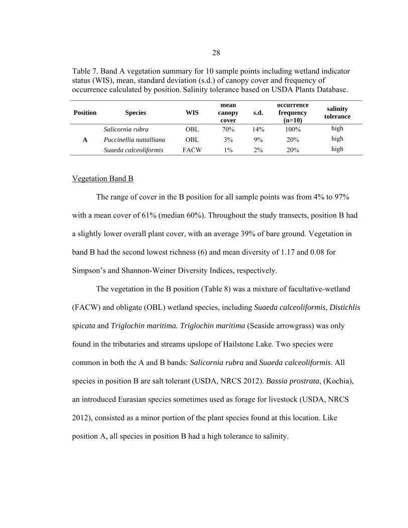
Table 7. Band A vegetation summary for 10 sample points including wetland indicator status (WIS), mean, standard deviation (s.d.) of canopy cover and frequency of occurrence calculated by position. Salinity tolerance based on USDA Plants Database.

Position Species WIS mean

canopy cover

s.d. occurrence frequency

(n=10)

salinity tolerance

A

Salicornia rubra OBL 70% 14% 100% high

Puccinellia nuttalliana OBL 3% 9% 20% high

Suaeda calceoliformis FACW 1% 2% 20% high

Vegetation Band B

The range of cover in the B position for all sample points was from 4% to 97%

with a mean cover of 61% (median 60%). Throughout the study transects, position B had

a slightly lower overall plant cover, with an average 39% of bare ground. Vegetation in

band B had the second lowest richness (6) and mean diversity of 1.17 and 0.08 for

Simpson’s and Shannon-Weiner Diversity Indices, respectively.

The vegetation in the B position (Table 8) was a mixture of facultative-wetland

(FACW) and obligate (OBL) wetland species, including Suaeda calceoliformis, Distichlis

spicata and Triglochin maritima. Triglochin maritima (Seaside arrowgrass) was only

found in the tributaries and streams upslope of Hailstone Lake. Two species were

common in both the A and B bands: Salicornia rubra and Suaeda calceoliformis. All

species in position B are salt tolerant (USDA, NRCS 2012). Bassia prostrata, (Kochia),

an introduced Eurasian species sometimes used as forage for livestock (USDA, NRCS

2012), consisted as a minor portion of the plant species found at this location. Like

position A, all species in position B had a high tolerance to salinity.

29

Table 8. Band B vegetation summary for 10 sample points including wetland indicator status (WIS), mean, standard deviation (s.d.) of canopy cover and frequency of occurrence calculated by position. Salinity tolerance based on USDA Plants Database.


canopy cover


(n=10)

salinity tolerance

B

Suaeda calceoliformis FACW 22% 30% 40% high

Triglochin maritima OBL 18% 39% 20% high

Distichlis spicata FACW 11% 29% 30% high



Bassia prostrata NI 1% 2% 10% high

Vegetation Band C

Thirteen species were found in the C position (Table 9). There were obligate

wetland species in this position but at a lower percent cover (12% OBL), compared to the

adjacent B and A positions. There was less bare ground than the neighboring B position

and the range of percent canopy cover in the C position for all sample points was 44% to

96% with a mean cover of 74% (median 80%). The C position vegetation was more

diverse than A and B positions with values of 1.79 and 0.28 for Simpson’s and Shannon-

Weiner Diversity Indices, respectively. Of the 13 species identified in the 10 position C

sample points, only 2 also occurred in both A and B vegetation bands, Salicornia rubra

and Puccinellia nuttalliana. The rhizomatous species, Distichlis spicata also occurred in

bands B and D. There was a range from high to low salinity tolerance among species in

position C.

30

Table 9. Band C vegetation summary for 10 sample points including wetland indicator status (WIS), mean, standard deviation (s.d.) of canopy cover and frequency of occurrence calculated by position. Salinity tolerance based on USDA Plants Database.


canopy cover


(n=10)

salinity tolerance

C


Thinopyrum intermedium UPL 11% 19% 30% medium

Poa pratensis FACU 10% 17% 40% low

Crepis runcinata FAC 8% 17% 20% medium

Bassia prostrata NI 7% 19% 20% high


Bromus arvensis FACU 6% 15% 20% low

unk. annual N/A 6% 19% 10% n/a


Mustard sp. NA 1% 3% 20% n/a

Hordeum jubatum FACW 1% 3% 10% high

Bromus tectorum UPL <1% 1% 10% low

Thlaspsi arvense UPL <1% 1% 10% medium

Vegetation Band D

Upland species dominated vegetation band D (Table 10). The range of percent

canopy cover for all sample points was from 64% to 100%, with a mean cover of 86%

(median 90%). Position D (like C) had a total species richness of 13 and the second

highest mean diversity with a value of 1.45 and 0.18 for Simpson’s and Shannon-Weiner

diversity indices, respectively. Distichlis spicata, Pascopyrum smithii, Alopecurus

arundinaceous, Hordeum jubatum are species known to have a high tolerance of salinity

(USDA, NRCS 2012) and 9 of the 13 species found in the D position are grasses.

Distichlis spicata, Thinopyrum intermedium, Poa pratensis, and Thlaspsi arvense are also

found in the C position. Bromus tectorum (cheatgrass) is considered invasive and

Onopordum (cotton thistle) is listed as non-native. Overall, there is less evenness of

31

species distribution among the 13 species in position D compared to the 13 species in

position C. There are more rare species (≤1% canopy cover) in position D (7) compared

to position C (5). Figure 8 depicts the mean percent bareground for all positions.

Table 10. Band D vegetation summary for 10 sample points including wetland indicator status (WIS), mean, standard deviation (s.d.) of canopy cover and frequency of occurrence calculated by position. Salinity tolerance based on USDA Plants Database.


canopy cover


(n=10)

salinity tolerance

D

Poa pratensis FACU 33% 39% 50% low


Thinopyrum intermedium UPL 10% 28% 30% medium

Poa secunda FAC 9% 29% 10% low

Pascopyrum smithii FACU 9% 25% 20% high

Alopecurus arundinaceus NI 6% 20% 10% high

Hordeum jubatum FACW 1% 3% 20% high

Lactuca serriola FACU 1% 2% 20% low

Bromus tectorum UPL 1% 3% 10% low

Bromus arvensis FACU <1% 1% 10% low

Thlaspsi arvense NI <1% 1% 10% medium

Medicago sativa NI <1% 1% 10% medium

Onopordum sp. NI <1% 1% 10% low

Plant Diversity

Table 11 shows mean plant diversity using two indices for each position (A-D).

The two indices were used to compare the effect of dominant species versus rare species.

Simpson’s index of diversity considers the number of species (richness), the proportion

of the assemblage occupied by each species (as percent cover) and gives more weight to

the most dominant species, as a result of squaring the proportion of each species

(Simpson 1949).

32

Figure 8. Percent bare ground by position within 10 transects at Hailstone National Wildlife Refuge. Error bars ± 1 standard deviation.

The Shannon-Weiner index gives more weight to rare species (Shannon 1948),

therefore the effective number of species from the Simpson index will always be less than

or equal to the effective number of species from the Shannon-Wiener index. The two

indices were proportionally equal and generally paralleled each other by position (Figure

9), which indicates that rare species did not affect the diversity in any position. C had the

highest mean plant diversity among positions regardless of either weighting scheme

followed by position D. Positions A and B have low diversity, lower richness and it can

be concluded that more species can tolerate environmental conditions in the higher

positions than are adaptable to the lower positions.

33

Table 11. Two diversity indices with richness (S), by vegetation band position.

Position Richness

(S) Inverse

Simpson’s (1/D)

Shannon-Wiener

(H’) A 3 1.12 0.05

B 6 1.17 0.08

C 13 1.79 0.28

D 13 1.45 0.18

Figure 9. Inverse Simpson’s and Shannon Wiener diversity indices plotted by position.

Wetland Indicator Status by Position

Table 12 shows the percentage cover and species richness (S) by vegetation type,

i.e., WIS, at positions A, B, C, and D. Obligate (OBL) and facultative wetland (FACW)

species have greater percentage canopy cover in the lower positions (A and B), and

upland plants (UPL) are denser (and more abundant) in drier positions. The distribution

and density among positions aligns with wetland plant indicator status assigned to the

various species for Region 4 (USDA, NRCS 2012).

Position

A B C D

Inve

rse

Sim

pso

n's

(1/D

)

1.0

1.2

1.4

1.6

1.8

2.0

Sha

nnon

Wie

ner

(H')

0.00

0.05

0.10

0.15

0.20

0.25

0.30

Simpson's Shannon-Wiener

34

Table 12. Vegetation type and mean percent coverage summary by bands A – D. s.d. indicates one standard deviation. (S) = species richness by WIS.

% Cover by Vegetation Type (WIS)

position OBL FACW FAC FACU UPL

mean s.d. (S) mean s.d. (S) mean s.d. (S) mean s.d. (S) mean s.d. (S)

A 74 12 ( 2 ) 1 2 ( 1 ) 0 0 ( 0 ) 0 0 ( 0 ) 0 0 ( 0 )

B 28 40 ( 3 ) 33 31 ( 2 ) 0 0 ( 0 ) 0 0 ( 0 ) 1 2 ( 1 )

C 8 19 ( 2 ) 16 25 ( 2 ) 8 17 ( 1 ) 16 21 ( 2 ) 26 27 ( 6 )

D 0 0 ( 0 ) 13 22 ( 2 ) 11 29 ( 1 ) 43 41 ( 3 ) 19 31 ( 7 )

Common Species within Bands

Characterization of plant assemblages using the most common species for

description and statistical analysis has been established in other studies (Sanderson et al.

2008). Most common species by position are shown in Table 13. Although present in

three positions, Salicornia rubra dominated the A position, whereas Distichlis spicata

was found in relatively even distribution across positions B, C and D. The overlap of

some species across vegetation bands may be reflective of species niche, and while

certain species dominated the bands, the vegetation in each band was not necessarily a

unique community type. The most common species among zones are discussed in detail.

Salicornia. Salicornia species (common name: glasswort, swamp samphire,

pickleweed) is a cosmopolitan genera native to North American, Europe, South Africa

and South Asia. They are a pioneer species and are included among a group of halophytes

35

Table 13. Prioritization of most common species for within-position analysis and these species were selected to represent their respective positions for later analysis. Mean and standard deviation (s.d.) are shown. Salinity tolerance based on USDA Plants Database.


canopy cover


salinity tolerance

A Salicornia rubra OBL 70% 14% 100% high

B Suaeda calceoliformis FACW 22% 30% 40% high

C Distichlis spicata FACW 16% 26% 30% high

D Poa pratensis FACU 33% 39% 50% low

that benefits from sodium concentrations above a level required as a micronutrient for a

majority of plants. Mahall (1976) found increased biomass production of Salicornia

species with increasingly saline waterlogged soils. Although they can tolerate a wide

range of salinities, they exhibit maximum growth at salinity of 10,000 mg/l

(approximately 12.5 dS/m) and are outcompeted in soils that lack salt (Zedler 1982;

Lewis 1982; Josselyn et al. 1983; Allison 1992). In addition, Noe and Zedler (2001)

found that extended spring rainfall may lead to increased germination as a result of

salinity dilution during the crucial emergence stage. Ungar et al. (1979) found that

competition determines the distributions of many halophytes and species interactions can

be especially affected by soil salinity levels. Although Salicornia species occur in

freshwater sediments (Griffith, unpublished data), it is easily outcompeted by plants

better adapted to such conditions (Mahall and Park 1976).

Salicornia rubra is a succulent chenopod (C4 plant), is commonly found in coastal

ecosystems as well as inland salty playas and saline seeps, and in USFWS Region 4, S.

rubra is an obligate wetland plant (OBL). It is an annual plant with a hermaphroditic

flower that is wind pollinated and contains a single seed (Flora of North America 1993).

36

Khan et al. (2001) found that S. rubra grew in concentric circles with other salt tolerant

species around a saltpan lake near Goshen, UT. This small annual forb was found nearest

the saltpan followed by the perennial forb, Salicornia utahensis. Pennings and Callaway

(1992) concluded that in a southern California salt marsh, competition was the factor

limiting establishment of S. rubra in the drier and more saline Arthrocnemum (Parish’s

glasswort) zone, but in a central California salt marsh, it was observed competing with

non-native upland plants (Wasson and Woolfolk 2011).

Suaeda calceoliformis. Like Salicornia rubra, Suaeda calceoliformis (common

name: Pursh seepweed, horned sea-blight), is a succulent halophyte and has been

documented to grow in areas of high soil salinity and alkalinity on areas identical to

Hailstone; playas, salt flats and other wetlands. It is an annual herb (C4 plant) and is more

common in higher salinity substrates when growing in a prostrate form, where it can

retain more water (Youngman and Heckathorn 1997). Suaeda calceoliformis is a FACW

plant in Region 4 (USDA, NRCS 2012).

Keiffer and Ungar (1997) conducted a germination study of Suaeda

calceoliformis (among others) by simulating seed exposure to high salinity. Two species

had a significant increase in the germination rate when compared to seeds germinated in

distilled water. Baseline germination data from seeds placed in 0, 1, 2, and 3% NaCl

solutions indicated that Salicornia europaea and Suaeda calceoliformis were the only

species to germinate in the 3% NaCl solution. The author concluded that prolonged

exposure to saline solutions can inhibit or stimulate germination in certain species and the

37

resulting germination and recovery responses are related to the duration and intensity of

their exposure to salt in their natural habitats.

Distichlis spicata. Distichlis spicata (saltgrass) is a halophytic graminoid (C4

plant) that inhabits upper/high marsh (irregularly flooded) areas, in which the water

levels vary between 5 cm above the soil surface and 15 cm below the soil surface. It is

also commonly present in the arid west, where it is one of the most drought-tolerant

species. Saltgrass is located in both organic alkaline and in saline soils (USDA, NRCS

2012). An important pioneer plant in early stages of succession in saline areas, the sharp-

pointed rhizomes of Distichlis spicata with its numerous epidermal silica cells, and the

aerenchymatous network of the rhizome, leaf sheath, and roots facilitate development of

the plant in anoxic conditions; heavy clays, shales, and inundated soils. In salt marshes of

southern Utah, Distichlis spicata contributes to a hummock-building process (increased

OM) that favors localized removal of salts by capillary action and evaporation. The

greatest amount of growth of Distichlis spicata takes place when temperatures are cool

and soil moisture is high during the early spring. During periods of high salt and water

stress, morphological and anatomical adaptations of saltgrass are important for survival

(Hansen et al. 1976). In a greenhouse investigation, Smart and Barko (1980) grew

Distichlis spicata from seed on freshwater, brackish and marine sediments. They found

that although the availability of nitrogen ultimately determined biomass accrual, sediment

salinity negatively affected growth rate.

38

Poa pratensis. Kentucky bluegrass is a cool-season perennial sod-forming grass

and is the only C3 plant of the four most common plants. The roots are shallow, often

within the upper 8 cm of the soil surface. Kentucky bluegrass is found most abundantly

on sites that are cool and humid. It has become naturalized across North America and

often occurs as a dominant species in the herbaceous layer. The active growth stage of

Poa pratensis begins in late winter/early spring and, by midsummer it is nearly dominant

on its sites. Cool temperatures in fall promote growth when other species are dying back.

It spreads by rhizomes, produces abundant seed, and can become established on disturbed

sites faster than other plant species. It is an aggressive competitor with native species and

has a low tolerance to salinity (USDA, NRCS 2012).

Vegetation and Position

Figure 10 shows the percent cover for the most common species across the four

positions. The composition of plant species occurring in bands may partially reflect

differences in the degree of adaptation to saturated conditions at Hailstone. For example

Salicornia rubra and Suaeda calceoliformis predominantly occupy wetter, lower A and B

positions, whereas Poa pratensis predominantly occupies the higher, drier D position.

The FACW species Distichlis spicata occurs in mesic and drier upslope positions and

seems to tolerate a wide range of growing conditions.

Conclusions

Vegetation communities on the shores at Hailstone appear to follow distinct,

patterns of colonization that generally follow the topography of the lakeshore. Vegetation

39

found at near-shoreline positions is predominantly wetland, salt-tolerant and

inundation/saturation-tolerant annual halophytes, with a single species dominating the

plant community (Figure 10). Moving away from the lake, vegetation occurs in repeated

patterns, with differences in amount of canopy cover, species diversity, and wetland

indicator status (WIS). The most common plant in the D position, Poa pratensis was the

only C3 plant of the four most common species, and the only species to have a low

tolerance to salinity. These findings are consistent with previously reported research

findings from sites similar to those observed at Hailstone National Wildlife Refuge.

Figure 10. Percent canopy cover across A-D positions for the four dominant species in each sample position at Hailstone National Wildlife Refuge.

40

Each position had a single predominant species and rare species had little effect

on diversity. The pattern of indices among positions, as calculated by two methods, was

nearly proportional, and diversity is greatest at position C, followed by position D.

Diversity was relatively low and similar for positions A and B. These data support the

conclusion that more commonly occurring species are adaptable to positions C and D,

farthest from the shoreline (and the abiotic conditions found there) than at positions A

and B. Vegetation establishment on positions A and B will likely be limited to only a

very few, select species, while on C and D substantially more species are capable of

establishing, offering a greater likelihood of success in vegetation establishment at these

positions. By comparing vegetation, it became evident that bands likely represented

similar abiotic environmental characteristics and further analysis was undertaken to

explore similarities or differences in abiotic conditions among vegetated bands.

41

ABIOTIC CONDTIONS OF A SALINE

LAKESHORE ENVIRONMENT

Abiotic conditions were compared among positions to determine whether salinity

and saturation vary significantly among vegetation bands that appear to radiate out from

the edges of the lake. This data was analyzed to whether these differences support the

occurrence of plants along a saturation/salinity gradient, based on their documented

tolerances.

Results

Landscape Characteristics

Sample point elevation above the lake water surface and depth to saturation were

examined for the 40 observation points at the Hailstone study site. Transect slope, length,

and sample point distance from the lake and/or channel bottom varied widely among

transects (Table 14). Vegetated banding occurred along transects of various lengths and

slopes and was a repeated visual feature regardless of these conditions.

Hydrology

Free-water in the sampling pits was a result of the presence of groundwater at a

point above the maximum depth of the pit. However because groundwater levels

fluctuate over time, indications of soil saturation were also documented. It should be

noted that presence of saturation does not indicate whether the uppermost level of

saturation was wicking upward or moving downward with lake dewatering.

42

Table 14. Length, height differential from point A to D in meters and mean slope for each transect. Slope equals height/length as a percentage. The distribution of the sample population is non-normal, 8 of 10 transect lengths are 25% or less of the maximum value. Mean, minimum, maximum and standard deviations (s.d.) are given to demonstrate the variability among transects.

Transect ID Length (m) Height (m) Slope

101 14.6 1.19 8.1%

102 10.1 0.49 4.9%

103 11.9 0.61 5.1%

104 10.7 0.73 6.8%

105 10.7 0.43 4.0%

106 96.9 1.28 1.3%

107 61.0 0.59 1.0%

108 24.4 1.05 4.3%

109 22.9 0.75 3.3%

110 26.5 0.46 1.7%

mean 29.0 0.8 2.6%

s.d. 28.3 0.3 2.3%

min 10.1 0.4 1.0%

max 96.9 1.3 8.1%

Table 15. Mean sample points distance (m) from water surface for each position; s.d. is one standard deviation. Sample points were not equally spaced across transects and were randomly chosen based on visual homogeneity of plant communities. The flatter transects had longer distances between sample points.

Sample position distance to water surface (m) A B C D

mean s.d. mean s.d. mean s.d. mean s.d.

1.13 1.84 9.52 8.47 18.90 19.46 30.08 27.65

Table 16 shows mean depth to saturation and standard deviation for all sample

points by position. Sample point elevation from the lake water surface is closely tied to

saturation depth as seen in Figure 11. As elevation of the sampling point increased (and

moved away from the water body), depth to saturation increased; concurrently, saturation

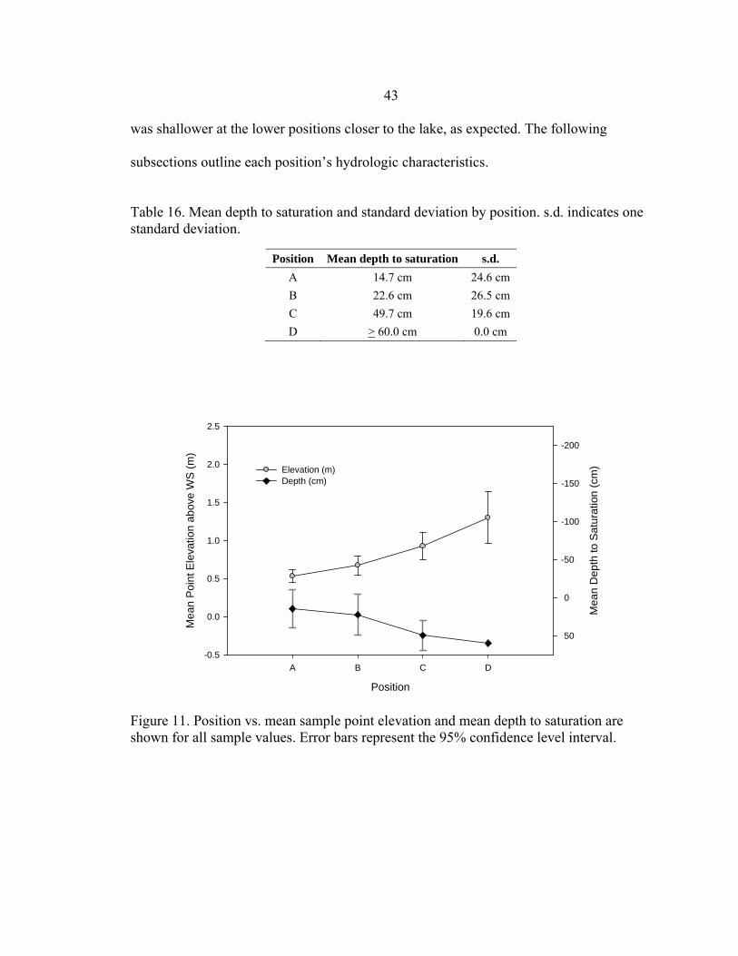
43

was shallower at the lower positions closer to the lake, as expected. The following

subsections outline each position’s hydrologic characteristics.

Table 16. Mean depth to saturation and standard deviation by position. s.d. indicates one standard deviation.

Position Mean depth to saturation s.d.

A 14.7 cm 24.6 cm

B 22.6 cm 26.5 cm

C 49.7 cm 19.6 cm

D > 60.0 cm 0.0 cm

Figure 11. Position vs. mean sample point elevation and mean depth to saturation are shown for all sample values. Error bars represent the 95% confidence level interval.

Position

A B C D

Mea

n P

oint

Ele

vatio

n ab

ove

WS

(m

)

-0.5

0.0

0.5

1.0

1.5

2.0

2.5

Mea

n D

epth

to S

atur

atio

n (

cm)

-200

-150

-100

-50

0

50

Elevation (m)Depth (cm)

44

Position A. In the A position, proximity to the lake influenced pit hydrology

(mean depth to saturation 14.7 cm, mean elevation above origin 7 cm). In observation

pits that had no free-water during the sampling period, other indications of wetting/drying

such as drift lines, oxidized root channels and water stained organic matter were

observed. Three pits in the A position had free-water which averaged 24 cm.

Position B. Like Position A, the proximity to the lake influenced hydrology in B

(median depth to saturation 10 cm, mean elevation above origin 24 cm) and there were

numerous indications of lake influence on the surface such as drift lines and water stained

organic matter. During sampling, the mean saturation depth was 22.6 cm and three pits in

the B position had free-water at an average depth of 35 cm.

Position C. This position had fewer hydrologic characteristics in common with the

two lower, wetter positions. Mean depth to saturation was approximately 50 cm (mean

Position C sample point elevation above WS: 45 cm), and there were fewer passive

indications of saturation or inundation at this position. In only one position C pit (102 C)

was free-water shallower than 60 cm during sampling (57 cm), and can likely be

explained by the close horizontal distance of this particular sample point to the lake (10

m). This sampling point was only 15 cm higher than the adjacent B position where depth

to saturation was 1 cm.

Position D. Position D is the upland position and all sample pits were dry. The

mean elevation of Position D sample points was 87 cm above lake water surface. There

was an absence of evidence indicating cyclic wetting-drying and/or aerobic-anaerobic

45

conditions and there were no passive hydrologic indicators such as drift lines or deposited

organic matter from the lake.

Soils

The soils at the sample sites are mapped primarily as Lardell clay loam (USDA,

NRCS 2012b). pH values among sample points and depths ranged from 6.8 to 9.5, and

were lowest at the upland positions, typical of semi-arid, calcareous soils of central

Montana. Percent OM (Figure 12) did not vary significantly between positions (F3, 156 =

2.287; p = 0.081). Differences in soil chemistry could be seen among positions and data

are reported by position.

Position A. Soils in Position A (Table 17) were characterized as saline-sodic

(mean EC0-2: 56 dS/m; average SAR0-2: 60) and at 20 cm, EC was 30 dS/m. pH and EC

differed significantly across the four depths (pH: F3, 36 = 8.016; p < 0.001. EC: F3, 36 =

8.074; p < 0.001). Position A had an average pH of 8.9 at the 0-5 cm horizon. Soil texture

was primarily sandy silt loam and had a predominance of redoximorphic features

providing evidence of seasonal inundation and saturation. Though reduction potential

was not quantitatively measured in this study, redox features indicated presence of anoxic

condition. Figure 13 shows a typical surface soil at Position A. The white crusts are

precipitated salts on the surface and the desiccated plants are Salicornia rubra from the

previous growing season.

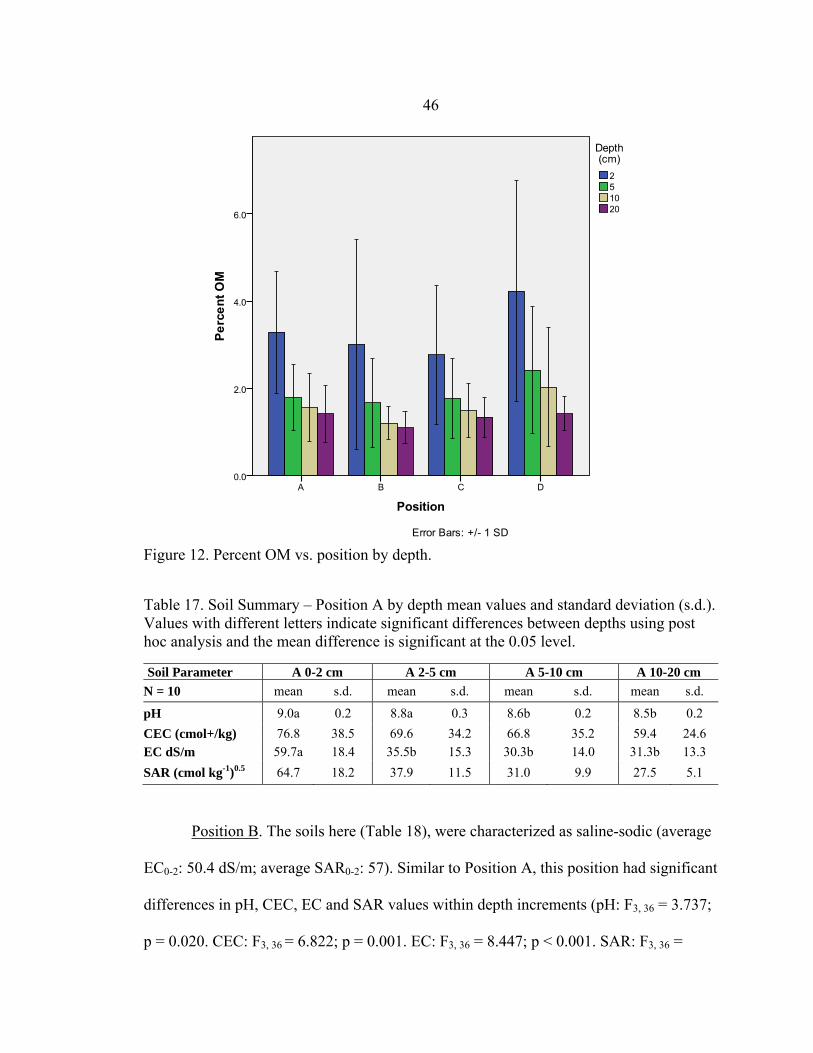
46

Figure 12. Percent OM vs. position by depth.

Table 17. Soil Summary – Position A by depth mean values and standard deviation (s.d.). Values with different letters indicate significant differences between depths using post hoc analysis and the mean difference is significant at the 0.05 level.

Soil Parameter A 0-2 cm A 2-5 cm A 5-10 cm A 10-20 cm

N = 10 mean s.d. mean s.d. mean s.d. mean s.d.

pH 9.0a 0.2 8.8a 0.3 8.6b 0.2 8.5b 0.2

CEC (cmol+/kg) 76.8 38.5 69.6 34.2 66.8 35.2 59.4 24.6 EC dS/m 59.7a 18.4 35.5b 15.3 30.3b 14.0 31.3b 13.3

SAR (cmol kg-1)0.5 64.7 18.2 37.9 11.5 31.0 9.9 27.5 5.1

Position B. The soils here (Table 18), were characterized as saline-sodic (average

EC0-2: 50.4 dS/m; average SAR0-2: 57). Similar to Position A, this position had significant

differences in pH, CEC, EC and SAR values within depth increments (pH: F3, 36 = 3.737;

p = 0.020. CEC: F3, 36 = 6.822; p = 0.001. EC: F3, 36 = 8.447; p < 0.001. SAR: F3, 36 =

47

16.839; p < 0.001). Soils in this position were primarily sandy silt loam and redox

features and saturated soil conditions indicated alternating wetting/drying,

aerobic/anaerobic, oxic/anoxic conditions. The average pH at the 0-5 cm horizon was 8.9.

Figure 13. Periodic soil-saturation results in the formation of mobile ferrous iron. The migrating groundwater redistributes the iron throughout the soil profile. During drainage, some areas around pores, cracks, and root channels become dry and aerated more quickly than the rest of the soil. Ferric iron precipitates in these places, forming reddish-brown spots. This pattern of spots or blotches of different color or a shade of color interspersed with the dominant color is called soil mottling (from Fletcher and Veneman 2012).

Table 18. Soil Summary – Position B mean values and standard deviation (s.d.). Values with different letters indicate significant differences between depths using post hoc analysis and the mean difference is significant at the 0.05 level.

Soil Parameter B 0-2 cm B 2-5 cm B 5-10 cm B 10-20 cm N = 10 mean s.d. mean s.d. mean s.d. mean s.d.

pH 9.0a 0.2 8.8ab 0.2 8.6b 0.3 8.7b 0.3

CEC (cmol+/kg) 79.7a 16.0 58.3b 18.5 53.5b 17.6 47.8b 15.3

EC dS/m 50.4a 17.4 28.5b 11.4 26.2b 11.2 24.9b 11.3

SAR (cmol kg-1)0.5 57.4a 18.5 31.2b 10.7 26.2b 9.8 21.9b 7.2

48

Position C. The Position C soils were characterized as saline-sodic (average

EC0-2: 14 dS/m; average SAR0-2: 18) but had a much lower level of salinity and sodicity

compared to Positions A and B. Unlike the two adjacent, lower positions, there was no

significant difference in EC values between depths (F3, 36 = 0.142; p = 0.934). Soils in

this position were primarily silt loam and had few visual redoximorphic features.

Compared to the Positions A and B, these soils were lower in soluble salts and sodium,

and had an average pH of approximately 8.4 in the 0-5 cm horizon. Table 19 summarizes

mean values for selected soil characteristics for Position C.

Table 19. Soil Summary – Position C mean values and standard deviation (s.d.). Values with different letters indicate significant differences between depths using post hoc analysis and the mean difference is significant at the 0.05 level.

Soil Parameter C 0-2 cm C 2-5 cm C 5-10 cm C 10-20 cm

N = 10 mean s.d. mean s.d. mean s.d. mean s.d. pH 8.43 .24 8.45 .24 8.45 .28 7.86 .44

CEC (cmol+/kg) 45.10 22.90 35.90 13.01 37.56 11.10 21.32 10.59

EC dS/m 14.02 12.48 12.20 6.82 12.05 5.11 4.19 4.87 SAR (cmol kg-1)0.5 17.7 16.7 16.8 11.6 17.3 9.0 19.6 8.5

Position D. There were significant differences in pH among depths in position D

(F3, 35 = 3.95; p = 0.016; Table 20). The soils here had an average EC0-2 of 4.2 dS/m and

an average SAR0-2 of 5.9, making them saline. There were no significant differences in

EC between depths; (F3, 35 = 1.596; p = 0.208), and there were no significant differences

in SAR levels between depths (F3, 35 = 2.469; p = 0.078). Soils in this position were

primarily silt loam and had no redoximorphic features. The soils in Position D were

comparatively neutral with an average pH of 7.9 at the 0-2 cm horizon. This position had

49

the highest content of organic matter (mean 4.7 % at 0-2 cm) compared to the averages of

the other three positions at the same depth.

Table 20. Soil Summary – Position D mean values and standard deviation (s.d.). Values with different letters indicate significant differences between depths using post hoc analysis and the mean difference is significant at the 0.05 level.

Soil Parameter D 0-2 cm D 2-5 cm D 5-10 cm D 10-20 cm

N = 10 mean s.d. mean s.d. mean s.d. mean s.d.

pH 7.9a 0.4 8.1ab 0.4 8.3bc 0.3 8.4c 0.3

CEC (cmol+/kg) 21.3 10.6 20.4 7.1 26.1 18.90 34.0 18.9 EC dS/m 4.2 4.9 5.0 4.60 6.9 5.2 9.0 5.1

SAR (cmol kg-1)0.5 5.9a 6.6 8.7ab 7.3 12.6ab 9.2 17.1b 12.4

Position, Saturation, and Salinity

ECdw by position are shown in Figure 14. In the A and B positions, EC is highest

on the soil surface compared to other depths. In the C and D positions, EC values are

similar throughout the entire soil column (as indicated by their relatively straight salinity

curves). Figure 15 shows mean EC depth profiles for all positions. All EC values by

position occupy a distinct location, from near shore to far, and from lower EC’s at pit

bottom to higher EC’s on the land surface. There is a bi-directional (vertical and

horizontal) salinity concentration gradient at positions A and B.

At Hailstone, soil saturation is a vector for solute transport. Saturated soil solution

EC and saturation depth are significantly correlated (r = -0.346, p < 0.001) across all

sample positions. Salinity and saturation follow a gradient from high soil EC and shallow

depth to saturation at Position A, to low soil EC and deep depth to saturation at Position

D. At the lower, wetter positions closer to the lake, the saturation/salinity profiles suggest

that solutes tend to move upward with wicking as driven by evaporation (resulting in

50

solute concentration at the surface) where at higher positions further from the lake,

solutes are moving slightly downward or laterally (see Figure 15).

Figure 14. Averaged depth-weighted EC among positions for all sample sites at Hailstone National Wildlife Refuge. Error bars represent 5% of the mean values.

Figure 15. EC depth profile by position. Mean point values and 5% error bars are shown for all sample values. EC values are highest at the surface, closest to the shoreline in positions A and B. At these positions, solutes are carried upward via evapoconcentration, and accumulate on the soil surface.

0.0 5.0 10.0 15.0 20.0 25.0 30.0 35.0 40.0

A

B

C

D

ECdw dS/m

Position

0

5

10

15

20

0 10 20 30 40 50 60

Depth (cm

)

Average EC (dS/m)

A

B

C

D

51

Nutrients Nutrient availability can affect the competitive dynamics between salt tolerant

plants and their position across environmental gradients in saturation stress (Emery et al.

2001). Primary macronutrients (N-P-K) concentrations for each position were examined

to determine whether nutrient concentrations might limit growth of vegetation at

Hailstone.

The levels of depth weighted N (F3, 36 = 1.55; p = 0.22), NO3 (F3, 36 = 1.44; p =

0.25), and NH4 (F3, 36 = 0.23; p = 0.83) did not differ across positions. Table 21 shows

depth-weighted means for all forms of nitrogen. The high cation exchange capacity

(CEC) in Hailstone soils may have also tied up plant available NH4, anoxic conditions in

lower positions may have increased atmospheric losses via denitrification, and given

relative concentrations of all forms, nitrogen may have been moderately limiting to plant

growth at the lower positions.

Table 21. Average depth weighted N, nitrate-N, and ammonium mean concentrations across all sampling positions.

Depth weighted mean

Position 1N mg/kg 2NO3 mg/kg 2NH4 mg/kg

A 2.9 2.7 6.9

B 2.8 2.9 6.1

C 6.3 10.0 6.2

D 3.7 5.4 7.3 1 was measured as exchangeable. 2 determined by saturated paste extraction (1:1 dilution).

52

Table 22 shows the means for total Pdw and the highly available plant available

orthophosphate (PO4) across all positions. Phosphorus was analyzed using the Bray 1

extraction method and because of higher pH levels, this method likely overestimated

plant available P. Total Pdw did not differ among positions (P: F3, 36 = 1.987; p = 0.133)

and PO4 levels did not differ among positions (F3, 36 = 1.393; p = 0.261). Phosphates

adsorb strongly to calcium carbonates (CaCO3), and at pH levels commonly found at

Hailstone, calcium carbonates can tie up large amounts of plant available P in the soil

(Jones and Jacobsen 2005b). Soil concentrations of PO4 are considered low for optimal

plant growth for all positions at Hailstone.

Table 22. Average depth weighted total P (Bray-1) and orthophosphate concentrations across all sampling positions. Values with different letters indicate significant differences between depths at the position.

Depth weighted mean

Position 1P mg/kg 2PO4 mg/kg

A 16.5a 0.6

B 11.0a 0.5

C 9.7b 0.4

D 11.4a 0.7 1 was measured as exchangeable. 2 determined by saturated paste extraction (1:1 dilution).

Potassium (K) concentrations in the soils at Hailstone averaged 236 mg/kg and

varied widely (min 115, max 401, s.d. 67 mg/kg). Mean differences did not exist between

positions (F3, 36 = 2.508; p = 0.074), and K levels may be considered normal for Montana

soils. Nevertheless, in soils with high levels of Ca and Mg, competition among exchange

sites can limit K uptake. K absorption is most limited by saturated soil conditions (Korb

et al. 2002), therefore actual plant available K may be limiting.

53

Depth-weighted Na levels by position are given in Table 23. Sodium levels were

significantly different among positions (F3, 36 = 12.428; p < 0.001) and post hoc tests

revealed significant differences between the two lowest positions (A and B) and C and D

(Table 23). Mean SARdw was significantly different along sample positions (F3, 36 =

10.958; p < 0.001).

Table 23. Average depth weighted potassium and sodium concentrations across all sampling positions. Values with different letters indicate significant differences between depths at the position.

Depth weighted mean

Position 1K mg/kg 2Na meq/L

A 227.2 4270.6a

B 205.3 3414.7a

C 232.4 2048.3b

D 280.9 1272.3b 1 was measured as exchangeable. 2 determined by saturated paste extraction (1:1 dilution).

Potassium and sodium are closely tied in their effects on osmoregulation in plant

tissues. In order to isolate Na and prevent root uptake in saline environments, plants use

K in abundance. In a study by Smart and Barko (1980), analysis of plant tissues and the

sediment interstitial water at the end of an investigation revealed selective uptake of

potassium and exclusion of sodium. These processes increased the ratio of sodium to

potassium in the interstitial waters and also resulted in increased sediment salinities

(Smart and Barko 1980).

54

Conclusions

The four positions (A-D) studied at Hailstone varied in their abiotic (length,

differential elevation and slope), soil chemistry and hydrologic characteristics. pH values

were highest at the A position, and the major nutrients did not vary across positions. EC

values were greater and depths to saturation were closer to the surface at positions closer

to the lake. This data suggests that point proximity to the lake determines soil salinity and

depth to saturation among the four positions and saturation and salinity are closely linked

at this environment. The connection between landscape position, soil chemistry and

hydrologic connectivity at Hailstone may be used to understand the presence of

environmental stress gradients and how plants grow near the lake and swales.

55

DISCUSSION

Synopsis

Vegetation grew in repeated patterns of plant assemblages, distinct from each

other, between the surface water and the upslope areas of Hailstone Lake. These plant

assemblages, appearing as banded growth patterns, were monotypic at some positions

relative to the lakeshore and consisting of mixed species at other positions relative to the

lakeshore. Sample points were chosen randomly within the four vegetated bands closest

to the lake, based on visual differences in vegetation type and density. Because of lake

basin topography, these sample points were distributed from a low elevation position, to

an outward and upward position from the lake depression and were labeled A through D.

Species richness was lowest at the A position (S=3), and was highest in positions C and

D (S=13). Species diversity was highest in the C position.

Depth to saturation was shallowest near the lakeshore and increased to ≥ 60 cm in

the upland D positions. Salinity (EC) was highest closest to the lake and incrementally

lower with adjacent positions away from the lakeshore. In positions A and B, salinity was

highest at the surface and decreased with depth (20 cm) and salinity (EC) and saturation

(depth) were correlated (r = -0.346, P < 0.001). The following conceptual model (Figure

16) represents the relationships between dominant vegetation and the abiotic

environmental characteristics that will be used as the basis for discussion.

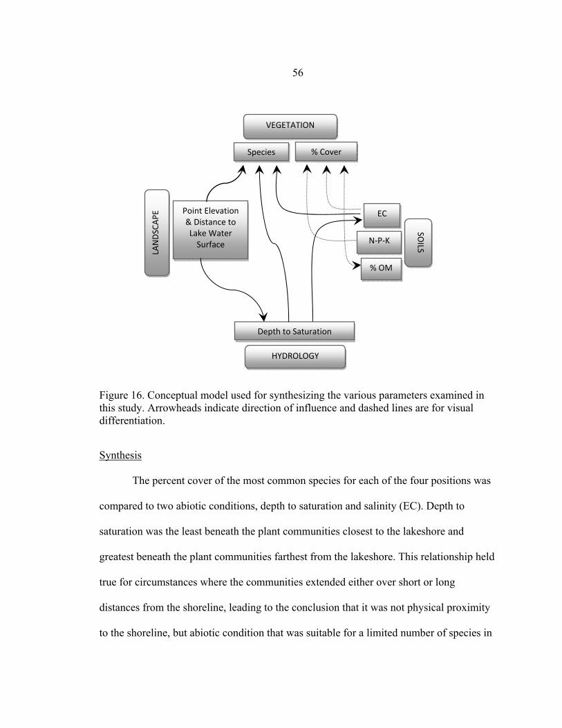
56

VEGETATION

Point Elevation & Distance to Lake Water Surface

% CoverSpecies LANDSCAPE EC

N‐P‐K

SOILS

% OM

Depth to Saturation

HYDROLOGY

Figure 16. Conceptual model used for synthesizing the various parameters examined in this study. Arrowheads indicate direction of influence and dashed lines are for visual differentiation.

Synthesis

The percent cover of the most common species for each of the four positions was

compared to two abiotic conditions, depth to saturation and salinity (EC). Depth to

saturation was the least beneath the plant communities closest to the lakeshore and

greatest beneath the plant communities farthest from the lakeshore. This relationship held

true for circumstances where the communities extended either over short or long

distances from the shoreline, leading to the conclusion that it was not physical proximity

to the shoreline, but abiotic condition that was suitable for a limited number of species in

57

some instances, i.e., positions A and B. These conditions likely represented the two most

stressful abiotic factors potentially affecting plant growth at Hailstone.

The A position was dominated by Salicornia rubra (OBL) but no other positions

had a single dominant species. S. rubra only occurred twice in position C and once in

position D. Salicornia rubra can be considered a pioneer species on the salty lakeshore.

As a short statured annual, it may have difficulty competing with perennial obligate

halophytes that also tolerate saturation and high salinity under circumstances which favor

alternate species to grow. In a personal observation, Puccinellia nuttalliana (Nuttall’s

alkaligrass) was found in higher abundance in the A positions (after field sampling) in

later months of 2010 and in 2011. Other factors (not explored in this study) may have

contributed to this condition including facilitation by Salicornia rubra, lower lake and

soil salinities during germination (as a result of above average precipitation in 2010 and

2011), and cooler springtime temperatures, which led to optimal establishment

conditions.

Suaeda calceoliformis (Pursh seepweed), the most abundant species in position B,

occurred in the wetter, more saline A position only twice (both points 4%) and did not

occur in the drier, higher C and D positions. The most abundant species in position C,

Distichlis spicata (inland saltgrass) can survive in areas of both fresh and salt waters

(lacunae tissue allows for gas exchange and survival in inundated conditions) and is also

one of the most drought-tolerant species in the dry, western interior of the United States

(Kitzes and Connor 2003). Its wide tolerance to wetness, drought, and salinity aligns with

its presence at Hailstone in a mesic position (C). Poa pratensis (Kentucky bluegrass)

58

does not tolerate extended anoxia and soil salinity (USDA, NRCS 2012) which makes it a

very good candidate for establishment and growth at the higher (elevational) position

along the saturation/salinity gradient within position D.

In the two years the study was conducted, the lower observation points (A and B)

were completely inundated in the spring. Moving away from the lake, saturation/salinity

stress was incrementally lower in positions C and D. These positions were occupied by

thirteen species apiece and had higher diversity. Based on these observations, the three

most prevalent species in positions A, B and D may be used to distinguish stress

gradients at Hailstone. Position C’s most abundant species, Distichlis spicata, grows well

along much of the saturation/salinity gradient, and, as a result, it is a difficult species for

which to characterize preferential soil chemistry and saturation tolerance alone on the

landscape. This species likely finds a niche within the mesic position as a result of

adaptation to salinity and saturation where other species cannot. Furthermore, even

though this species is extremely well adapted to a wide range of conditions, it most often

occurs in distinct bands across the study plots at Hailstone.

Lower positions may experience a different type of abiotic (physical) stress: wave

action and ice scour/deposition, which could inhibit seedling establishment, survival,

and/or growth, resulting in lower density and species richness. In the A position

Salicornia rubra may be less affected by harsh winter conditions as an annual plant, and

in the C position the highly rhizomatous saltgrass may be able to tolerate physical

scouring. Steeper slopes may be more affected by wave action whereas longer, flatter

transects tend to attenuate and dissipate wave energy across a longer distance.

59

Given the open and flat landscape of Hailstone, there are likely only small

differences in solar insolation (albeit without field measurement) that would affect plant

growth. This circumstance likely normalizes the differences in evapotranspiration, solar

gain, heat units, etc., at the landscape scale. However, based on anecdotal observations of

the effects shading/surface roughness has on the growth of plants, these factors may play

a critical role in lowering sun and wind driven evaporation, reducing soil temperature,

and generally conserving moisture at the plant scale.

Biotic Factors. The effects of competition and facilitation should not go

unmentioned in the process of vegetation zonation. Hacker and Gaines (1997) described

an increase in species diversity at the harsh end of the environmental stress gradient

because of facilitation; species colonize areas where they would not normally be able to

tolerate as a result of benefit derived from the presence of other species. This was not

observed at the A position at Hailstone and the lack of observed facilitation there may be

a result of the extreme salinities found in the lake and along the lakeshore. Facilitation

may be more of a factor in determining species diversity in the B and C positions where

salinities are reduced. Nevertheless, organic matter inputs from the accumulation of

biomass may alleviate the negative effects of salinity as well as change the hydrologic

response of precipitation inundation via preferential flow along rooting channels.

Applications

Figure 17 shows a scatter plot of ECdw with distance to the origin (lake).

Although this data represents a bimodal data distribution (i.e., 36 of the values cluster

60

between 0 and 30 m from the water and 4 values, 3 of which are < 10, fall more than 40

m out from the water), it represents a salinity gradient that took many years to develop.

The final location of the restored Hailstone Creek will ultimately drive the formation of a

new salinity/saturation gradient that will likely look much different from that of the

existing shoreline, based on years of submersion by highly saline waters. Salinity profiles

may not vary much along similar transect lengths, and it may take many human

generations for stable profiles to develop as fresh rainwater pushes surface salts

downward in the highest positions, or as wicking drives salinity upward in the lowest

areas. Hailstone Creek salinity will also affect soil salinities in the areas adjacent to the

stream.

Figure 18 shows the mean ECdw values of the two shortest, steepest transects and

two longest, flattest transects. These data suggest that there is no difference in depth

weighted ECdw between short-steep and long-flat slope at positions C or D. There are

larger differences in ECdw between the two transects types at the A and B positions. This

may be indicative of longer seasonal inundation (and solute residence time) at the lower

positions in the long-flatter transects.

In the absence of detailed depth to saturation and salinity data across much of the

exposed lakebed, lakebed elevation from the water (Hailstone Creek) may be a useful

metric to predict potential plant responses to altered hydrology. Combined with the data

from this study and a small number of field measurements, a conceptual design for

revegetation planning could be generated.

61

Figure 17. Scatter plot of depth weighted EC and distance from the origin (lake). The trend line (exponential) shows that ECdw values decrease with increasing distance from lake.

Figure 18. Mean depth weighted EC for short transects vs. long transects by position. Error bars represent 5 % value.

R² = 0.3340

10

20

30

40

50

60

70

0 20 40 60 80 100 120

ECdw dS/m

Distance from lake (m)

0.0 10.0 20.0 30.0 40.0 50.0

A

B

C

D

Mean EC (dS/m)

Position

short‐steep

flat‐long

62

Based on salinity/saturation and vegetation by position, the advancement of

conceptual revegetation zones is put forth here. Zonation determination in this conceptual

model was based on several assumptions:

1) As shown in the data, saturation is closely tied to salinity and will be an important

factor in determining species germination, establishment and long term survival. It is

uncertain at what location lakebed saturation will equilibrate with stream water and

groundwater (as tied to the influence of the surrounding geohydrology) until the effects

of dewatering are fully realized.

2) Following the evacuation of a majority of lake water in 2011, a single soil sample

was taken from the exposed lakebed between the A position and the new water surface on

the western shoreline. Soil ECdw, was approximately 32 dS/m, a value that fell between

the A and B positions from the 2010 study. It is important to emphasize that actual soil

salinities may vary across the lakebed and can only be confirmed by multiple samples. It

is assumed in this model that the newly exposed lakebed will likely have soil salinities

close to the single 2011 sample point which is similar to the salinities found at the 2010

A and B study positions.

3) It is unlikely that salinity conditions found at the study position D will be found at

any location on the exposed lakebed. Only through slow movement of salts downward

with precipitation will the exposed landscape return to an upland environment

comparable to the D position, therefore, conceptual revegetation zones contain species

only found in positions A through C. Some species observed in this study are considered

invasive or have deleterious effects to livestock. The use of these species or additional

63

species not found on the site, but having potential reclamation application, should be

reviewed by USFWS botanists prior to initiation of revegetation activities.

4) At the time of this writing, conditions at Hailstone were not conducive to vehicle

traffic on the lakebed. It is unknown to what extent conditions will improve based on soil

drainage patterns and groundwater influences on soil stability. These conditions will

affect the type of revegetation techniques that can be deployed on site. In addition, certain

constituents in the soil and water are toxic to humans (selenium) and a thorough analysis

of their mobilization, transport and fate should be understood prior to exposing personnel

to disturbed soils.

The primary criteria used for establishment of zones were projections and assumptions of

developing salinity and saturation conditions. Table 24 outlines the depth to saturated soil

and ECdw values for each proposed zone. The justification for each zone was based

broadly on the primary abiotic conditions observed during the 2010 field study between

positions A, B and C. The threshold values for depth to saturation and ECdw between

zones are very broad and meant to be a general guideline. In some instances, these model

parameters should be adjusted for actual field conditions. For instance, if there are areas

of surface saturation within Zone 3, OBL plants not listed for that zone should be used

within the saturated area.

Table 25 outlines the 9 species recommended for planting in 3 zones. These

species are a mix of the most salt tolerant native plants found on the A, B and C positions

during the study and was the first criterion used for selection. The next criterion used was

adaptation to anoxia/saturation and the selected species were positioned within their

64

respective zones in terms of their relative tolerance of this condition. Figure 19 shows a

lakebed profile with revegetation zones in order to illustrate their position and relative

elevation on the lakebed surface.

Table 24. Hailstone salinity/saturation conditions by revegetation zone.

Revegetation Zone

Depth to Saturation (cm)

ECdw (dS/m)

1 < 15 > 30 2 15 – 30 25 ± 5 3 30 - 60 < 20

Table 25. Hailstone vegetation guide by zone. Species shown are only those found in the species pool in this study and some species are recommended in more than one zone. The use of introduced and invasive species may or may not be practicable, only as allowed by USFWS management. N=native, I=introduced, H=high salt tolerance, M=medium salt tolerance.

Revegetation Zone

Species WIS Native Status

Saline Toler.

1

Salicornia rubra OBL N H

Puccinellia nuttalliana OBL N H

Triglochin maritima OBL N H

2 Suaeda calceoliformis FACW N H

Triglochin maritima OBL N H

Distichlis spicata FACW N H

Hordeum jubatum FACW N H

3

Distichlis spicata FACW N H

Pascopyrum smithii UPL N H

Alopecurus arundinaceus NI I H

Thinopyrum intermedium UPL I M

Revegetation Zone 1. This zone is closest to the restored Hailstone Creek and will

be most similar in hydrology to Position A. There will likely be a wetted perimeter

extending along the margins of the creek and backwater channels. Depths to saturation in

65

this zone must support obligate wetland species of plants and therefore should be within

15 cm of the soil surface as was found in Position A in the 2010 study. The width of the

wetted perimeter that will support obligate wetland species will likely vary depending on

streambank slope, and although the stream is now slow moving, solute residence time

may be shorter in this zone than that found in position A, depending on seasonal

precipitation patterns and flushing. In contrast to the increasing and constant salinization

within the lake, seasonal flushing may lower salinities (compared to existing conditions)

along the wetted perimeter of the creek. Ultimately, source water salinities will drive

accumulation or flushing of salts from the streambank soils. If salinities are lower during

crucial germination periods (seasonal high-water), conditions may favor species such as

Puccinellia nuttalliana. This obligate wetland species is well adapted to all soil types, has

high tolerance to anoxia, does not require a cold stratification and grows in a wide range

of soil pH (USDA, NRCS 2012). Triglochin maritima has also been selected for use in

Zone 1 as a result of its observed rooting potential in the swale sample transects. This

species may be a good candidate for streambank slope stabilization but, this species is

also is known for producing cyanogenic compounds (prussic acid) in the mesophyll cells

(leaf tissues) and may be harmful to livestock (NDSU 2012).

Revegetation Zone 2. As discussed, soil salinities may be relatively homogenous

across the new lakebed and expected EC levels throughout Zone 2 will be similar to Zone

1. Unlike the lower zone, saturation will likely be deeper here (15-30 cm) and plants must

be more adapted to these hydrologic conditions, yet still have high tolerance to salinity.

Species selected for this zone will overlap with Zones 1 and 3 and depending on actual

66

topography (and relative depth to groundwater) this zone may vary widely in species

composition. The first three species have been discussed previously in detail and their

ecologic characteristics are well suited for this position. The last species, Hordeum

jubatum is a facultative wetland plant that has a high tolerance to salinity, a wide range of

moisture regimes and pH levels. Hordeum jubatum is a pioneer species and rapidly

invades areas exposed by a receding water table (USDA, NRCS 2012). This is a native

species and has been found useful in reclamation of saline lands, but is considered a

weedy species and has been identified to be harmful to wildlife and livestock as a result

of its upward-pointing barb-like awns becoming easily embedded into an animal’s tissue,

causing irritation. These less desirable traits should be carefully weighed against potential

reclamation benefits prior to widespread use, but it is likely that this plant will colonize

naturally at Hailstone.

Revegetation Zone 3. This zone will be limited to plants that can tolerate both arid

and saline conditions. As discussed previously, obligate and facultative wetland, salt

tolerant plants are able to utilize the available water in order to osmoregulate tissue turgor

and function optimally, but at Zone 3, water will not likely be available at depths

shallower than 60 cm (post-dewatering). The most stressful end of the environmental

gradient may eventually be found here. Species chosen for this zone have characteristics

of salinity tolerance as well as some adaptation to drier conditions. Distichlis spicata has

been discussed in detail and this species will likely be a primary candidate across the

entire site for revegetation. Alopecurus arundinaceus is an introduced cultivar that has a

high rate of spread and can be invasive. It may be a useful species because of its highly

67

rhizomatous roots and high tolerance to salinity. Western wheatgrass (Pascopyrum

smithii) has been shown to tolerate high salinities and a wide range of soil pH, and is

moderately tolerant of anoxic conditions (USDA NRCS 2012). It is a rhizomatous plant

and has a rapid rate of growth. In conjunction with intermediate wheatgrass (Thinopyrum

intermedium), these species can provide decent forage for wildlife and livestock.

Thinopyrum intermedium may be most suited for the highest positions on the lakebed as

it has the lowest tolerance to salinity of all chosen species (medium).

Figure 19. Revegetation profile for three zones. Distance from stream varies by location.

Figure 20 depicts a preliminary revegetation model for three planting zones based

on a land and lake bathymetry survey (Ducks Unlimited 2009). Revegetation zones were

generally based on the predicted lakebed elevations from Hailstone Creek as related to

depth to groundwater. It cannot be overemphasized that confirmation of depth to

saturation should be made prior to initiating any revegetation planting.

Reveg Zone1S. rubra

P. nuttallianaT. maritima

Reveg Zone 2S. calceoliformisT. maritimaD. spicataH. jubatum

Reveg Zone 3D. spicata

A. arundinaceusP. smithii

T. intermedium

0.00

0.50

1.00

1.50

2.00

2.50

3.00

Elevation from

stream (m)

Distance from stream (m)

68

Figure 20. A conceptual map of revegetation zones based on digital elevation modeling using lake bathymetry and land survey points to predict hydrologic response to dewatering and partial dam removal.

69

The newly exposed lakebed will be difficult to access by machinery and people

while sediments drain and dry. Places close to the creek and tributaries may be

indefinitely unrealistic to access as a result of persistent saturation. A large-scale

revegetation effort may also be unrealistic in terms of available financial resources.

Therefore, phased treatments should be considered. As opposed to a large scale seeding,

smaller ‘islands’ or banded patterns of vegetation should be considered (Figure 21). Once

established, these areas may encourage OM accumulation and natural spreading of

vegetation. Utilization of limited fresh-water precipitation and organic matter

accumulation (leaf litter) by islands or bands will facilitate further plant growth by

enhancing root macropore development and infiltration (salt flushing). Increasing surface

roughness also assists in aeolian deposition of OM and seed. Vegetated bands could be

positioned at inflow seeps, perpendicular to the slope to intercept incoming water.

Surface runoff intercepted by these bands will become run-on and infiltrate water on the

up-slope side. The band may move gradually upslope as OM accumulates. Bare areas

between bands or islands will be smoother and form soil crusts and these inter-canopy

areas will allow rainfall to flow downslope into other bands and infiltrate beneath the

larger plants. The larger plants will harvest rainfall from the ground immediately up-

slope (Tongway and Ludwig 2001).

As allowable, larger plant sizes (pre-grown containerized nursery stock) should be

used as a method of increasing plant establishment. Deeper roots in a containerized plant

may have access to soil depths where salinities are lower and supporting soil water is

present. Supplemental OM along with soil manipulation (roughening) and creation of

70

shade-inducing structures should also be considered to enhance growth performance in

focused revegetation areas. These treatments may be most important and relevant in

Revegetation Zone 3 where soil moisture is lowest and salinities are high.

Figure 21. Example of vegetated islands and banding within Revegetation Zones 2 and 3.

Conclusions

At Hailstone Lake, up-gradient saline seeps, eighty years of impounded lake

water and the lack of precipitation have resulted in exacerbated soil and water

salinization. In this study, I learned that the four positions varied in their physical, soil

chemistry and hydrologic characteristics. The connection between landscape position,

71

soil chemistry and hydrology were used to understand the presence of plant distributions.

Vegetation responds to soil salinity and saturation levels, and it is likely that the banded

growth patterns are indicative of a combination of the stress tolerance of the individual

species and their ability to colonize, occupy, or compete for suitable sites (e.g. higher

diversity of species found in C and D positions).

Environmental stress gradients in plant community ecology have been studied in

detail and abiotic environmental stress (e.g. prolonged saturation/anoxia and high

salinity, drought, extreme cold) is a primary cause of lower species richness (Keddy

1989; Engels 2010). Where species’ distributions overlap, biotic factors such as

interspecies competition may be important in determining the observed banding patterns.

Although not a focus of this study, biotic effects of competition and facilitation almost

certainly play a role in vegetation assemblage formation at Hailstone, particularly at

positions C and D. Ultimately, understanding salinity and saturation conditions will likely

determine what suite of plants will be most appropriate to focus on future revegetation

efforts.

The information elucidated in this study can be used to stabilize and revegetate

landscapes impacted by saline seep, abandoned saline-sodic lakebeds and other denuded

lands. Halophytes, selected for a high degree of salinity tolerance, could be grown

specifically for the planting on the exposed lakebed, and when guided by predicted

saturation/salinity conditions as modeled from existing data sources, could provide for

long term establishment of vegetation. The challenge in performing these activities under

a yet unknown hydrologic regime must not go unmentioned. Nevertheless, understanding

72

the nature of fluctuating hydrology, plant ecophysiology and saline soil chemistry,

coupled with the use of selected plant materials on the newly exposed lakebed, could

increase the potential for revegetation success over time.

73

REFERENCES

Abrol, I. P., Yadav, J. S. P., Massoud, F.I. (1988). Salt-Affected Soils and Their Management. Rome, Food and Agriculture Organization of the United Nations.

Allison, S. K. (1992). The influence of rainfall variability on the species composition of a

northern salt marsh plant assemblage. Vegetation. 101(2): 145-160. Barrett-Lennard, E. (2002). "Restoration of saline land through revegetation."

Agricultural Water Management 53(1-3): 213-226. Bauder, J. (2010). Pesonal communication, Hailstone project discussion, Montana State

University, Bozeman MT. [email protected]. Bertness, M. D. and Callaway, R. (1994). "Positive interactions in communities." Trends

in Ecology & Evolution 9: 191-193. Bertness, M. D. and Ellison, A. M. (1987). "Determinants of pattern in a New England

salt marsh plant community." Ecological Monographs 57(2): 129-147. Biology Online (2012). Zonation definition. Accessed March 19, 2012.

http://www.biology-online.org/dictionary/Zonation. Costa, C. S. B., Marangoni, J. C., Azeveda, A.M.G. (2003). "Plant zonation in irregularly

flooded salt marshes: Relative importance of stress tolerance and biological interactions." Journal of Ecology 91(6): 951-965.

Cowardin, L. M. (1978). "Wetland classification in the United States." Journal of

Forestry 76(10): 666-668. Crow Tribe, Official Site of the. (2012). "History of the Apsáalooke." Accessed April 25,

2012. http://www.crowtribe.com/history.htm. Dorn, R. D.(1984). Vascular Plants of Montana. Mountain West Publishing, Cheyenne,

WY. 276 p. Ducks Unlimited. (2009). Lake bathymetry and ground survey data. Used by permission. Emery, N. C., Ewanchuk, P. J., Bertness, M.D. (2001). "Competition and salt-marsh plant

zonation: stress tolerators may be dominant competitors." Ecology 82(9): 2471-2485.

74

Engels, J. A. (2010). Drivers of marsh plant zonation and diversity patterns along estuarine stress gradients. Ph.D, University of Hamburg.

Fletcher, P. and Veneman, P. (2012). "Soil morphology as an indicator of seasonal high

water tables." Accessed November 14, 2011. http://nesoil.com/properties/eshwt.htm.

Flora of North America Editorial Committee. (1993). Flora of North America: North of

Mexico. New York, Oxford University Press. Flowers, T. J., Troke, P. F., Yeo, A.R. (1977). "The mechanism of salt tolerance in

halophytes." Annual Review of Plant Physiology 28: 89-121. Giri, B. and Mukeriji, K. G. (2004). "Mycorrhizal inoculant alleviates salt stress in

Sesbania aegyptiaca and Sesbnia grandiflora under field conditions: Evidence for reduced sodium and improved magnesium uptake." Mycorrhiza 14: 307-312.

Gleick, P. H. (1993). "Water and conflict - fresh water resources and international

security." International Security 18(1): 79-112. Glenn, E. P., Brown, J. J., Blumwald, E. (1999). "Salt tolerance and crop potential of

halophytes." Critical Review Plant Science 18: 227-255. Griffith, K. A. Unpublished data. (2009). The interacting effects of salinity and nutrient

additions to pickleweed and dodder. Univeristy of California, Santa Cruz. [email protected].

Hacker, S. D. and Gaines, S. D. (1997). "Some implications of direct positive interactions

for community species diversity." Ecology 78: 1990-2003. Hansen, D. J., Dayanandan, P., Kaufman, P.B., Brotherson, J.D. (1976). "Ecological

adaptations of salt marsh grass, Distichlis spicata (Gramineae), and environmental factors affecting its growth and distribution." American Journal of Botany 63(5): 635-650.

Hasegawa, P. M., Bressan, R. A., Zhu, J, Bohnert, H. J. (2000). Plant cellular and

molecular responses to high salinity. Annual Review of Physiology and Plant Molecular Biology. 51:463-99.

Herrera, A. (2008). "Crassulacean acid metabolism and fitness under water deficit stress:

If not for carbon gain, what is facultative CAM good for?" Annals of Botany 103(4): 645-653.

75

Holzer, J., Miller, M. R., Brown, S.K., Leagare, R.G., Von Stien, J.J. (1995). Dryland salinity problems in the Great Plains of Montana: Hydrogeology aspects and control programs. International Association of Hydrogeologists Congress XXVI-Drylands Salinity, Edmonton, AB Canada.

Horsnell, T. K., Smettem, K. R. J., Reynolds, D. A., Mattiske, E. (2009). "Composition

and relative health of remnant vegetation fringing lakes along a salinity and waterlogging gradient." Wetlands Ecology and Management 17(5): 489-502.

Jones, C., Jacobsen, J. (2005a). Plant nutrition and soil fertility. Nutrient Mangement

Module No. 2. Montana State University Extension Service Publication 4449-2. Jones, C., Jacobsen, J. (2005b). Phosphorus cycling, testing and fertilier

recommendations. Nutrient Mangement Module No. 4. Montana State University Extension Service Publication 4449-4.

Josselyn, M., National Coastal Ecosystems Team (U.S.), United States Army Corps of

Engineers. (1983). The ecology of San Francisco Bay tidal marshes: A community profile. Washington, D.C.

Keddy, P. A. (1989). "Effects of competition from shrubs on herbaceous wetland plants:

A four year field experiment." Canadian Journal of Botany 67: 708-716. Keiffer, C. H. and Ungar, I. A. (1997). "The effect of extedned exposure to hypersaline

conditions on the germination of five inland halophyte species." American Journal of Botany 84(1): 104-111.

Kellogg, S. P. (1984). An overviewof saline seeps in stillwater county. S. C. District: 46. Kering, M. K. (2008). Manganese nutrition and photosynthesis in NAD-malic enzyme C4

plants Ph.D. dissertation. Ph.D, University of Missouri-Columbia. Khan, M.A., Gul, B. Weber, D. J. (2001). "Effect of salinity on the growth of ion content

of Salicornia rubra." Communications in Soil Science and Plant Analysis. 32(17): 2965-2977.

Kitzes, J. and Connor, J. (2003). "Distichlis spicata." Marine Botany. Accessed March 4,

2012. http://www.mbari.org/staff/conn/botany/seagrass/justin/index.htm. Korb, N. A., Jones, C., Jacobsen, J. (2002). Potassium cycling, testing and fertilizer

recommendations. Nutrient Management Module No. 5. MSU Extension Sevice, MSU: 12 p.

76

Lewis, M., Clark, W., Moulton, G. E., Dunlay, T. W., (2002). The definitive journals of Lewis & Clark. Lincoln, University of Nebraska Press.

Lewis, R. R. (1982). Creation and Restoration of Coastal Plant Communities. CRC Press

Boca Raton, FL. 219 p. Lopez, D. A. (2000). Geologic Map of the Billings 30' x 60' Quadrangle, Montana,

Montana Bureau of Mines and Geology: Geologic Map 59, 51:100,000. Mahall, B. E. and Park, R. B. (1976). "Ecotone between Spartina foliosa Trin. and

Salicornia virginica L. in salt marshes of northern San Fransisco Bay." Journal of Ecology 64(3): 793-809.

Manousaki, E. and Kalogerakios, N. (2011). "Halophytes - An emerging trend in

phytoremediation." International Journal of Phytoremediation 13(10) 959-969. McCauley, A., and Jones, C. (2005). Salinity and sodicity managment. Soil and Water

Management Module 2. Montana State University Extension Service Publications 4481-2.

McFarlane, D. J. and Williamson, D. R. (2002). "An overview of waterlogging and

salinity in southwestern Australia as related to the ‘Ucarro’ experimental catchment." Agricultural Water Management 53(1-3): 5-29.

Miller, M. R., Donovan, J., Bergantino, R.N., Sonderegger, J. L., Schmidt, F. A. (1980).

Saline-seep development and control in the North American Great Plains: hydrogeological aspects. Montana Bureau of Mines and Geology 4: 15-23.

Mitsch, W. J. and Gosselink, J. G. (2007). Wetlands. Hoboken, N.J., Wiley. Mozafar, A. and Goodin, J. R. (1970). "Vesiculated hairs - A mechanism for salt

tolerance in Atriplex halimus L." Plant Physiology 45(1): 62-65. NDSU. (2012). Prussic acid poisoning. North Dakota State University Department of

Agriculutre V-1150. Accessed April 12, 2012. http://www.ag.ndsu.edu/pubs/ansci/livestoc/v1150w.htm.

Nelson, D., Rammesmayer, G., Bohnert, H. J. (1998). "Regulation of cell-specific

inositol metabolism and transport in plant salinity tolerance." Plant Cell 10(5): 753-764.

Nelson, K. J. and Reiten, J. C. (2009). "Saline seep impacts on Hailstone and Halfbreed

National Wildlife Refuges in south-central Montana." US Fish and Wildlife Service Report.

77

Nilsen, E. T., Orcutt, D. M., Hale, M. G. (1996). The Physiology of Plants Under Stress.

Vol 1: Abiotic Factors. 689 pp. New York, Wiley. NOAA. (2011). "Total Growing Degree Days (corn)." Accessed December 29, 2011.

http://www.cpc.ncep.noaa.gov/products/analysis_monitoring/cdus/degree_days/grodgree.txt.

Noe, G. and Zedler, J. (2001). "Variable rainfall limits the germination of upper intertidal

marsh plants in southern California." Estuaries 24(1): 30-40. Pennings, S. C. and Callaway, R. M. (1992). "Salt marsh plant zonation - The relative

importance of competition and physical factors." Ecology 73(2): 681-690. Ramadan, T. (1998). "Ecophysiology of salt excretion in the xero-halophyte Reaumuria

hirtella." New Phytologist 139(2): 273-281. Rand, T. A. (2000). "Seed dispersal, habitat suitability and the distribution of halophytes

across a salt marsh tidal gradient." Journal of Ecology 88: 608-621. Reed, P.B. (1988). National List of Plant Species That Occur in Wetlands: National

Summary. U.S. Fisha and Wildlife Service. Rep 88(24). 244 pp. Rhodes, D., Nodolska-Orczyk, A. (2001). Plant Stress Physiology. Encyclopedia of Life

Sciences. Nature Publishing Group. Sanderson, J. S., Kotliar, N. B., Steingraeber, D. A. (2008). "Opposing environmental

gradients govern vegetation zonation in an intermountain playa." Wetlands 28(4): 1060-1070.

Sandoval, F. M. and Gould, W. L. (1978). Improvement of saline- and sodium-

affected disturbed lands. Reclamation of Drastically Disturbed Lands. pp 485-504. Madison, WI, American Society of Agronomy.

Schlyer, K. W (2007). Defenders of Wildlife. America's 10 most endangered wildlife

refuges 2007. Refuges at Risk. p 8. Shamsutdinov, N. Z. and Shamsutdinov, Z. (2009). Halophytes usage for soil desalting

and sustainable development of agriculture in arid regions of Russia. Kostyakov All-Russian Research Institute of Hydraulic Engineering and Land Reclamation.

Shannon, C. E. (1948). "A mathematical theory of communication." Bell System

Technical Journal 27: 379-423 and 623-656.

78

Shevyakova, N., Netronina, I., Aronova, E. E., Kuznetsov, V.V. (2003). "Compartmentation of cadmium and iron in Mesembryanthemum crystallinum plants during the adaptation to cadmium stress." Russian Journal of Plant Physiology 50(5): 678-685.

Simpson, E. H. (1949). "Measurement of Diversity." Nature 163: 688. Smart, M. R. and Barko, J. W. (1980). "Nitrogen nutrition and salinity tolerance of

Distichlis spicata and Spartina alterniflora." Ecology 61(3): 630-638. Snow, A. A. and Vince, S. W. (1984). "Plant zonation in an Alaskan salt marsh . An

experimental study of the role of edaphic conditions." Journal of Ecology 72(2): 669-684.

Stewart, R. E. and Kantrud, H. A. (1971). Classification of natural ponds and lakes in the

glaciated prairie region. Washington, U.S. Bureau of Sport Fisheries and Wildlife. Resource Publication 92: 57 pp.

Subbarao, G. V., Ito, O., Berry, W. L., Wheeler, R. M. (2003). "Sodium: A functional

plant nutrient." Critical Reviews in Plant Sciences 22(5): 391-416. Tester, M. and Davenport, R. (2003). "Na+ tolerance and Na+ transport in higher plants."

Annals of Botany 91(5): 503-527. Thein, S. J. (1979). Soil Texture by Feel. Journal of Agronomy Education. K. S.

University Extension Publication MF-2243. Thorne, D. W. and Peterson, H. B. (1949). Irrigated soils, their fertility and management.

Philadelphia, Blakiston Co. 288 pp. Tiner, R. W. (1991). "The concept of a hydrophyte for wetland identification - Individual

plants adapt to wet environments." Bioscience 41(4): 236-247. Tongway, D. J. and Ludwig, J. A. (2001). Theories on the origins, maintenance,

dynamics and functioning of banded landscapes. In, Banded vegetation patterning in arid and semiarid environments: ecological processes and consequences for management, ed. D. J. Tongway, C. Valenin, and J. Segheri, pp 20-31. Springer-Verlag, New York.

Ungar, I. A., Benner, D. K., McGraw, D. C. (1979). "Distribution and growth of

Salicornia europaea on an inland saltpan." Ecology 60(2): 329-336. USDA, NRCS. (1991). Management of saline/sodic soils. Accessed March 22, 2011.

http://www.nrcs.usda.gov/Internet/FSE_DOCUMENTS/stelprdb1044792.pdf.

79

USDA, NRCS. (2010). Field Indicators of Hydric Soils in the United States,

Version 7.0. L.M. Vasilas, G.W. Hurt, and C.V. Noble (eds.). USDA, NRCS, in cooperation with the National Technical Committee for Hydric Soils.

USDA, NRCS. (2012). The PLANTS Database. National Plant Data Team, Greensboro, NC 27401-4901. Accessed March 23, 2012. http://plants.usda.gov.

USDA, NRCS. (2012b). Web Soil Survey. Stillwater County Area, Montana (MT655).

Accessed March 24, 2012. http://websoilsurvey.nrcs.usda.gov/app/HomePage.htm.

USFWS (1988). Wetland Indicator Categories U.S. USFWS Biological Report 88 [26.9]

1988, Revised 1993. Wasson, K. and Woolfolk, A. (2011). "Salt marsh-upland ecotones in central California:

Vulnerability to invasions and anthropogenic stressors." Wetlands 31(2): 1-14. Whitson, T. D., (1991). Weeds of the West. Western Society of Weed Science X. 630 p. Wickens, G. E. (1989). Economic Halophytes - A Global Review, Springer. WRCC, (2011). LCD Summaries for the Western US. Accessed December 5, 2011.

http://www.wrcc.dri.edu/summary/bil.mt.html. Youngman, A. L. and Heckathorn, S. A. (1992). "Effect of salinity on water relations of

two growth forms of Suaeda calceoliformis." Functional Ecology 6(6): 686-692. Zedler, J. B. (1982). The ecology of southern California coastal salt marshes: a

community profile. Washington, D.C., U.S. Fish & Wildlife Service, FWS/OBS-81/54, 110 pp.

Zhu, J. K. (2001). "Plant salt tolerance." Trends in Plant Science 6(2): 66-71.

80

APPENDICES

81

APPENDIX A

VEGETATION PERCENT COVER

Vegetation Percent Cover

S rub

P nut

T mar

D spi

H jub

L lat

S calc

P pra

B jap

C run

L ser

K pro

T int

B tec

P smi

A lyr

T arv

M sat

Ono A aru

must Ann A cri S het

101A 0.56 0 0 0 0 0 0 0 0 0 0 0 0 0 0 0 0 0 0 0 0 0 0 0

102A 0.48 0.28 0 0 0 0 0 0 0 0 0 0 0 0 0 0 0 0 0 0 0 0 0 0

103A 0.56 0 0 0 0 0 0 0 0 0 0 0 0 0 0 0 0 0 0 0 0 0 0 0

104A 0.72 0 0 0 0 0 0 0 0 0 0 0 0 0 0 0 0 0 0 0 0 0 0 0

105C 0.92 0.04 0 0 0 0 0 0 0 0 0 0 0 0 0 0 0 0 0 0 0 0 0 0

106A 0.76 0 0 0 0 0 0.04 0 0 0 0 0 0 0 0 0 0 0 0 0 0 0 0 0

107A 0.8 0 0 0 0 0 0 0 0 0 0 0 0 0 0 0 0 0 0 0 0 0 0 0

108A 0.84 0 0 0 0 0 0 0 0 0 0 0 0 0 0 0 0 0 0 0 0 0 0 0

109A 0.76 0 0 0 0 0 0 0 0 0 0 0 0 0 0 0 0 0 0 0 0 0 0 0

110A 0.64 0 0 0 0 0 0.04 0 0 0 0 0 0 0 0 0 0 0 0 0 0 0 0 0

101B 0 0 0 0.92 0 0 0 0 0 0 0 0.05 0 0 0 0 0 0 0 0 0 0 0 0

102B 0 0 0 0.16 0 0 0 0 0 0 0 0 0 0 0 0 0 0 0 0 0 0 0 0

103B 0.44 0.24 0 0 0 0 0 0 0 0 0 0 0 0 0 0 0 0 0 0 0 0 0 0

104B 0 0 0.88 0.04 0 0 0 0 0 0 0 0 0 0 0 0 0 0 0 0 0 0 0 0

105B 0.04 0 0 0 0 0 0 0 0 0 0 0 0 0 0 0 0 0 0 0 0 0 0 0

106B 0.04 0 0 0 0 0 0.36 0 0 0 0 0 0 0 0 0 0 0 0 0 0 0 0 0

107B 0.12 0.04 0 0 0 0 0.68 0 0 0 0 0 0 0 0 0 0 0 0 0 0 0 0 0

108B 0 0 0.96 0 0 0 0 0 0 0 0 0 0 0 0 0 0 0 0 0 0 0 0 0

109B 0 0 0 0 0 0 0.4 0 0 0 0 0 0 0 0 0 0 0 0 0 0 0 0 0

110B 0 0 0 0 0 0 0.72 0 0 0 0 0 0 0 0 0 0 0 0 0 0 0 0 0

101C 0 0 0 0 0 0 0 0.24 0.2 j 0 0 0 0 0 0 0 0 0 0 0 0 0 0

102C 0 0.6 0 0 0 0 0 0 0 0 0 0 0.32 0 0 0 0 0 0 0 0 0 0 0

103C 0.02 0 0 0.44 0 0 0 0 0 0 0 0.08 0 0 0 0 0 0 0 0 0 0 0 0

104C 0 0 0 0 0 0 0 0.04 0 0.28 0 0 0.28 0 0 0 0 0 0 0 0 0 0 0

105E 0 0 0 0 0.08 0 0 0.24 0 0 0 0 0.52 0.04 0 0 0 0 0 0 0 0 0 0

106C 0 0 0 0.68 0 0 0 0 0 0 0 0 0 0 0 0 0 0 0 0 0.02 0 0 0

107C 0.12 0 0 0 0 0 0 0 0 0 0 0.6 0 0 0 0 0 0 0 0 0.08 0 0 0

108C 0 0 0 0 0 0 0 0.48 0 0.48 0 0 0 0 0 0 0 0 0 0 0 0 0 0

82

109C 0 0 0 0.44 0 0 0 0 0.44 0 0 0 0 0 0 0 0.04 0 0 0 0 0 0 0

110C 0 0.04 0 0 0 0 0 0 0 0 0 0 0 0 0 0 0 0 0 0 0 0.6 0 0

101D 0 0 0 0 0 0 0 0.92 0 0 0 0 0 0 0 0 0 0 0.02 0 0 0 0 0

102D 0 0 0 0 0 0 0 0 0 0 0 0 0 0 0.8 0 0 0 0 0 0 0 0 0

103D 0 0 0 0 0 0 0 0 0 0.16 0 0 0 0 0 0 0 0 0 0.64 0 0 0 0

104D 0 0 0 0 0.08 0 0 0.8 0 0 0 0 0.08 0 0 0 0 0 0 0 0 0 0 0

105A 0 0 0 0.32 0 0 0 0.24 0 0 0 0 0 0.08 0 0 0 0 0 0 0 0 0 0

106D 0 0 0 0 0 0 0 0.92 0 0 0 0 0.04 0 0 0 0 0 0 0 0 0 0 0

107D 0 0 0 0.6 0 0 0 0 0.04 0 0.04 0 0 0 0 0 0 0 0 0 0 0 0 0

108D 0 0 0 0.28 0.04 0 0 0.6 0 0 0.04 0 0 0 0 0 0 0.04 0 0 0 0 0 0

109D 0 0 0 0 0 0 0 0.76 0 0 0 0 0 0 0.12 0 0.04 0 0 0 0 0 0 0

110D 0 0 0 0 0 0 0 0 0 0 0 0 0.88 0 0 0 0 0 0 0 0 0 0 0

count if 16 6 2 9 3 0 6 10 3 3 2 3 6 2 2 0 2 1 1 1 2 1 0 0

freq 0.35 0.13 0.04 0.20 0.07 0.00 0.13 0.22 0.07 0.07 0.04 0.07 0.13 0.04 0.04 0.00 0.04 0.02 0.02 0.02 0.04 0.02 0.00 0.00

83

84

APPENDIX B

TABLES OF STATISTICAL ANALYSIS

85

Tables of Statistical Analysis

ANOVA

Dependent Variable: OM pct

Source df F Sig.

Corrected Model 3 2.287 .081

Intercept 1 313.308 .000

Position 3 2.287 .081

Error 156

Total 160

Corrected Total 159

a. R Squared = .042 (Adjusted R Squared = .024)

Levene's Test of Equality of Error Variancesa

Dependent Variable:OM_pct

F df1 df2 Sig.

13.475 3 156 .000

Tests the null hypothesis that the error variance

of the dependent variable is equal across groups.

a. Design: Intercept + Depth_cm

Position A - pH x depth

ANOVA

Dependent Variable:pH

Source df F Sig.

Depth_cm 3 8.016 .000

Error 36

Total 40

Corrected Total 39

86

ANOVA


Source df F Sig.

Depth_cm 3 8.016 .000

Error 36

Total 40

Corrected Total 39


Multiple Comparisons

pH

LSD

(I) Depth_cm (J) Depth_cm

Mean Difference

(I-J) Sig.

2 3 .150 .138

5 .350* .001

10 .440* .000

3 2 -.150 .138

5 .200 .051

10 .290* .006

5 2 -.350* .001

3 -.200 .051

10 .090 .369

10 2 -.440* .000

3 -.290* .006

5 -.090 .369

Based on observed means.

The error term is Mean Square(Error) = .049.

*. The mean difference is significant at the 0.05 level.

87

A – EC x Depth

Tests of Between-Subjects Effects

Dependent Variable: EC

Source df F Sig.

Depth_cm 3 8.074 .000

Error 36

Total 40

Corrected Total 39



EC

LSD


Mean Difference

(I-J) Sig.

2 3 24.130* .001

5 29.402* .000

10 28.323* .000

3 2 -24.130* .001

5 5.272 .449

10 4.193 .546

5 2 -29.402* .000

3 -5.272 .449

10 -1.079 .876

10 2 -28.323* .000

3 -4.193 .546

5 1.079 .876


The error term is Mean Square(Error) = 236.922.

88


EC

LSD


Mean Difference

(I-J) Sig.

2 3 24.130* .001

5 29.402* .000

10 28.323* .000

3 2 -24.130* .001

5 5.272 .449

10 4.193 .546

5 2 -29.402* .000

3 -5.272 .449

10 -1.079 .876

10 2 -28.323* .000

3 -4.193 .546

5 1.079 .876




A – CEC x Depth

ANOVA

Dependent Variable: CEC

Source df F Sig.

Depth_cm 3 .458 .713

Error 36

Total 40

Corrected Total 39

89

ANOVA


Source df F Sig.

Depth_cm 3 .458 .713

Error 36

Total 40

Corrected Total 39

a. R Squared = .037 (Adjusted R Squared = -.044)

SARdw by Position

ANOVA

Dependent Variable: SAR_DW

Source df F Sig.

Position 3 10.958 .000

Error 36

Total 40

Corrected Total 39



SAR_DW

LSD

(I) Position (J) Position

Mean

Difference (I-J) Sig.

A B 5.730 .148

C 15.220* .000

D 20.070* .000

90

B A -5.730 .148

C 9.490* .019

D 14.340* .001

C A -15.220* .000

B -9.490* .019

D 4.850 .219

D A -20.070* .000

B -14.340* .001

C -4.850 .219



*. The mean difference is significant at the .05 level.

A – SAR x depth


Dependent Variable:SAR

F df1 df2 Sig.

6.753 3 36 .001



a. Design: Intercept + Depth_cm

91

Position B- pH x depth

ANOVA


Source df F Sig.

Depth_cm 3 3.737 .020

Error 36

Total 40

Corrected Total 39



pH

LSD


Mean Difference

(I-J) Sig.

2 3 .230 .059

5 .360* .004

10 .320* .010

3 2 -.230 .059

5 .130 .277

10 .090 .450

5 2 -.360* .004

3 -.130 .277

10 -.040 .736

10 2 -.320* .010

3 -.090 .450

5 .040 .736



92


pH

LSD


Mean Difference

(I-J) Sig.

2 3 .230 .059

5 .360* .004

10 .320* .010

3 2 -.230 .059

5 .130 .277

10 .090 .450

5 2 -.360* .004

3 -.130 .277

10 -.040 .736

10 2 -.320* .010

3 -.090 .450

5 .040 .736




B – CEC x depth

ANOVA


Source df F Sig.

Depth_cm 3 6.822 .001

Error 36

Total 40

Corrected Total 39

93

ANOVA


Source df F Sig.

Depth_cm 3 6.822 .001

Error 36

Total 40

Corrected Total 39



CEC

LSD


Mean Difference

(I-J) Sig.

2 3 21.430* .007

5 26.260* .001

10 32.000* .000

3 2 -21.430* .007

5 4.830 .527

10 10.570 .171

5 2 -26.260* .001

3 -4.830 .527

10 5.740 .453

10 2 -32.000* .000

3 -10.570 .171

5 -5.740 .453




94

B – EC x depth

ANOVA


Source df F Sig.

Depth_cm 3 8.447 .000

Error 36

Total 40

Corrected Total 39



EC

LSD


Mean Difference

(I-J) Sig.

2 3 21.923* .001

5 24.168* .000

10 25.532* .000

3 2 -21.923* .001

5 2.245 .704

10 3.609 .541

5 2 -24.168* .000

3 -2.245 .704

10 1.364 .817

10 2 -25.532* .000

3 -3.609 .541

5 -1.364 .817




95

B- SAR x depth

ANOVA

Dependent Variable: SAR

Source df F Sig.

Depth_cm 3 16.839 .000

Error 36

Total 40

Corrected Total 39



SAR

LSD


Mean Difference

(I-J) Sig.

2 3 26.194* .000

5 31.148* .000

10 35.465* .000

3 2 -26.194* .000

5 4.954 .373

10 9.271 .100

5 2 -31.148* .000

3 -4.954 .373

10 4.317 .437

10 2 -35.465* .000

3 -9.271 .100

5 -4.317 .437



96


SAR

LSD


Mean Difference

(I-J) Sig.

2 3 26.194* .000

5 31.148* .000

10 35.465* .000

3 2 -26.194* .000

5 4.954 .373

10 9.271 .100

5 2 -31.148* .000

3 -4.954 .373

10 4.317 .437

10 2 -35.465* .000

3 -9.271 .100

5 -4.317 .437




Position C- pH x depth

ANOVA


Source df F Sig.

Depth_cm 3 .140 .935

Error 36

Total 40

Corrected Total 39


97

C - CEC x depth

ANOVA


Source df F Sig.

Depth_cm 3 1.162 .338

Error 36

Total 40

Corrected Total 39


C- EC x depth



Source df F Sig.

Depth_cm 3 .142 .934

Error 36

Total 40

Corrected Total 39


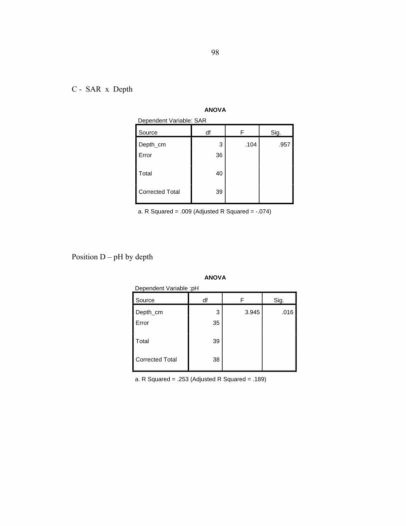
98

C - SAR x Depth

ANOVA


Source df F Sig.

Depth_cm 3 .104 .957

Error 36

Total 40

Corrected Total 39


Position D – pH by depth

ANOVA

Dependent Variable :pH

Source df F Sig.

Depth_cm 3 3.945 .016

Error 35

Total 39

Corrected Total 38


99


pH

LSD


Mean Difference

(I-J) Sig.

2 3 -.102 .484

5 -.322* .032

10 -.442* .004

3 2 .102 .484

5 -.220 .127

10 -.340* .021

5 2 .322* .032

3 .220 .127

10 -.120 .400

10 2 .442* .004

3 .340* .021

5 .120 .400




D - CEC x depth

ANOVA

Dependent Variable:CEC

Source df F Sig.

Depth_cm 3 2.353 .089

Error 35

Total 39

Corrected Total 38


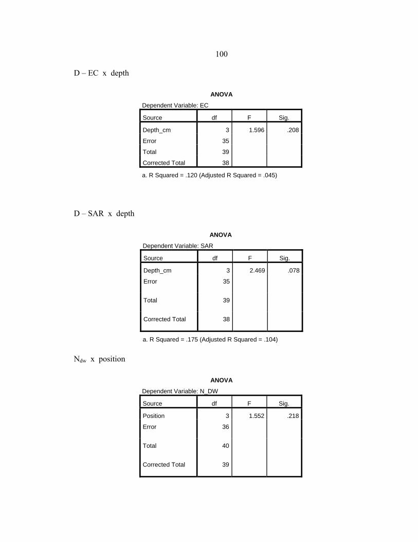
100

D – EC x depth

ANOVA


Source df F Sig.

Depth_cm 3 1.596 .208

Error 35

Total 39

Corrected Total 38


D – SAR x depth

ANOVA


Source df F Sig.

Depth_cm 3 2.469 .078

Error 35

Total 39

Corrected Total 38


Ndw x position

ANOVA

Dependent Variable: N_DW

Source df F Sig.

Position 3 1.552 .218

Error 36

Total 40

Corrected Total 39

101

ANOVA

Dependent Variable: N_DW

Source df F Sig.

Position 3 1.552 .218

Error 36

Total 40

Corrected Total 39


NO3dw x position


Dependent Variable:NO3_DW

Source df F Sig.

Position 3 1.439 .248

Error 36

Total 40

Corrected Total 39


102

NH4 dw x Position

ANOVA

Dependent Variable: NH4_DW

Source df F Sig.

Position 3 .292 .831

Error 36

Total 40

Corrected Total 39


Position N mg/kg NO3 mg/kg Position NH4 mg/kg

Aa

0-2 cm A mean 4.3 8.8

A

10.9

s.d. 6.1 16.6 6.4

2-5 cm A mean 2.8 3.3 6.6

s.d. 1.2 2.8 3.3

5-10 cm A mean 2.5 2.1 6.3

s.d. 0.7 1.0 2.7

10-20 cm A mean 2.8 1.7 6.4

s.d. 1.0 0.8 3.5

Ba 0-2 cm B mean 4.2 6.1

B 9.2

s.d. 4.0 6.5 3.3

103

2-5 cm B mean 3.1 3.1 5.7

s.d. 2.2 3.0 2.4

5-10 cm B mean 2.6 2.5 5.0

s.d. 1.1 2.3 1.6

10-20 cm B mean 2.6 2.5 6.2

s.d. 1.1 2.2 2.4

Cb

0-2 cm C mean 12.6 20.2

C

9.9

s.d. 14.6 25.7 5.3

2-5 cm C mean 7.5 13.0 6.6

s.d. 7.8 18.3 3.4

5-10 cm C mean 6.3 9.5 5.9

s.d. 8.3 15.5 2.5

10-20 cm C mean 4.6 7.3 5.5

s.d. 5.4 13.8 2.1

Dab

0-2 cm D mean 6.2 11.2

D

14.0

s.d. 4.8 10.7 18.0

2-5 cm D mean 4.1 6.9 7.8

s.d. 3.4 7.2 7.0

5-10 cm D mean 3.6 4.9 7.0

s.d. 2.7 6.1 5.0

10-20 cm D mean 3.2 4.0 5.9

s.d. 3.2 6.7 2.3

104

Phosphorus

P mg/kg PO4 mg/kg

Aa

0-2 cm A mean 29.3 2.3

s.d. 14.0 1.0

2-5 cm A mean 17.1 0.6

s.d. 5.3 0.5

5-10 cm A mean 14.1 0.5

s.d. 5.2 0.4

10-20 cm A mean 15.0 0.4

Ba

s.d. 7.1 0.3

0-2 cm B mean 22.9 1.7

s.d. 17.3 1.5

2-5 cm B mean 14.0 0.5

s.d. 9.4 0.3

5-10 cm B mean 9.4 0.4

s.d. 6.1 0.2

10-20 cm B mean 8.5 0.3

C

s.d. 5.0 0.2

0-2 cm C mean 22.4 1.2

s.d. 15.3 1.2

2-5 cm C mean 12.2 0.4

s.d. 8.4 0.3

5-10 cm C mean 8.6 0.4

s.d. 6.5 0.2

10-20 cm C mean 7.0 0.3

105

Da

s.d. 4.7 0.2

0-2 cm D mean 26.0 1.5

s.d. 18.6 1.1

2-5 cm D mean 15.5 0.9

s.d. 10.6 0.7

5-10 cm D mean 10.4 0.7

s.d. 7.5 0.6

10-20 cm D mean 7.8 0.5

s.d. 7.8 0.3

Pdw by position

ANOVA

Dependent Variable: P_DW

Source df F Sig.

Position 3 1.987 .133

Error 36

Total 40

Corrected Total 39


106

PO4 dw x position

ANOVA

Dependent Variable: PO4_DW

Source df F Sig.

Position 3 1.393 .261

Error 36

Total 40

Corrected Total 39


Kdw by position

ANOVA

Dependent Variable: K_DW

Source df F Sig.

Position 3 2.508 .074

Error 36

Total 40

Corrected Total 39


107

K mg/kg Na mg/kg

Aa

0-2 cm A mean 254.0

A

5630.6

s.d. 71.5 3167.9

2-5 cm A mean 226.1 4381.9

s.d. 62.4 1903.2

5-10 cm A mean 232.1 4251.2

s.d. 68.8 2065.1

10-20 cm A mean 219.8 3975.0

s.d. 62.7 1781.1

Ba

0-2 cm B mean 274.4

B

4634.8

s.d. 92.8 1049.1

2-5 cm B mean 229.0 3617.5

s.d. 92.6 934.9

5-10 cm B mean 204.0 3307.1

s.d. 80.9 1116.7

10-20 cm B mean 185.0 3163.6

s.d. 66.1 1201.0

Ca

0-2 cm C mean 288.8

C

1797.1

s.d. 63.3 1355.4

2-5 cm C mean 253.7 1830.5

s.d. 50.8 1186.0

5-10 cm C mean 237.8 1972.5

s.d. 58.8 1018.9

10-20 cm C mean 212.1 2201.7

s.d. 52.2 1027.1

D 0-2 cm D mean 333.2 D 513.4

108

s.d. 118.2 685.9

2-5 cm D mean 321.7 716.3

s.d. 117.7 632.2

5-10 cm D mean 298.0 1187.7

s.d. 60.8 963.4

10-20 cm D mean 249.7 1633.1

s.d. 64.4 1093.3

Na dw by position

ANOVA

Dependent Variable:Na_DW

Source df F Sig.

Position 3 12.428 .000

Error 36

Total 40

Corrected Total 39



Na_DW

LSD

(I) Position (J) Position

Mean

Difference (I-J) Sig.

A B 855.960 .121

C 2222.390* .000

D 2998.370* .000

B A -855.960 .121

C 1366.430* .016

109

D 2142.410* .000

C A -2222.390* .000

B -1366.430* .016

D 775.980 .159

D A -2998.370* .000

B -2142.410* .000

C -775.980 .159





Dependent Variable: EC_DW

F df1 df2 Sig.

5.036 3 36 .005



a. Design: Intercept + Position

Correlations

Saturation_Depth EC

Saturation_Depth Pearson Correlation 1 -.346**

Sig. (2-tailed) .000

N 160 160

EC Pearson Correlation -.346** 1


N 160 160

**. Correlation is significant at the 0.01 level (2-tailed).

110

Correlations

depth_saturation

Sal_rub Pearson Correlation -.497**


N 40

Sua_calc Pearson Correlation .173


N 40

Dist_spic Pearson Correlation .056


N 40

Poa_pra Pearson Correlation .291


N 40

**. Correlation is significant at the 0.01 level (2-tailed).

Correlations

EC_0-2 cm

Sal_rub Pearson Correlation .665**


N 40

Sua_calc Pearson Correlation .315*


N 40

Dist_spic Pearson Correlation -.229


N 40

Poa_pra Pearson Correlation -.429**


N 40

111

Correlations

EC_0-2 cm

Sal_rub Pearson Correlation .665**


N 40

Sua_calc Pearson Correlation .315*


N 40

Dist_spic Pearson Correlation -.229


N 40

Poa_pra Pearson Correlation -.429**


N 40

**. Correlation is significant at the 0.01 level (2-

tailed).

*. Correlation is significant at the 0.05 level (2-

tailed).

Documents

SOILS, HYDROLOGY AND VEGETATION DISTRIBUTION by