Soil Moisture Active Passive (SMAP) Project Assessment

1

Soil Moisture Active Passive (SMAP) Project Assessment Report for the L2SMSP

Beta-Release Data Products Citation: Das, Narendra N., D. Entekhabi, S. Dunbar, S. Kim, S. Yueh, A. Colliander, T. J. Jackson, P. E. O’Neill, M. Cosh, T. Caldwell, J. Walker, A. Berg, T. Rowlandson, J. Martínez-Fernández, Á. González-Zamora, P. Starks, C. Holifield-Collins, J. Prueger, and E. Lopez-Baeza, November 1, 2017. Assessment Report for the L2_SM_SP Beta Release Data Products, SMAP Project, JPL D-56549, Jet Propulsion Laboratory, Pasadena, CA.

Paper copies of this document may not be current and should not be relied on for official purposes. The current version is in the Product Data Management System (PDMS): https://pdms.jpl.nasa.gov/ Nov 1, 2017

JPL D-56549

National Aeronautics and Space Administration

Jet Propulsion Laboratory 4800 Oak Grove Drive Pasadena, California 91109-8099 California Institute of Technology

© 2017 California Institute of Technology. Government sponsorship acknowledged.

2

Contributors to this report: Das, Narendra.1, D. Entekhabi2, S. Dunbar1, S. Kim1, S. Yueh1, A. Colliander1, T. J. Jackson3, P. E. O’Neill4, M. Cosh3, T. Caldwell5, J. Walker6, A. Berg7, T. Rowlandson8, J. Martínez-Fernández9, Á. González-Zamora9, P. Starks10, C. Holifield-Collins11, J. Prueger12, and E. Lopez-Baeza13

1Jet Propulsion Laboratory, California Institute of Technology, Pasadena, CA 91109 USA

2Massachusetts Institute of Technology, Cambridge, MA 02139 USA 3USDA ARS Hydrology and Remote Sensing Lab, Beltsville, MD 20705 USA 5Goddard Space Flight Center, NASA, Greenbelt, MD 20771, USA 5University of Texas, Austin, TX 78713 USA 6Monash University, Clayton, Australia 7University of Guelph, Guelph, Canada 8Comisión Nacional de Actividades Espaciales (CONAE), Buenos Aires, Argentina 9University of Salamanca, Salamanca, Spain 10USDA ARS Grazinglands Research Laboratory, El Reno, OK 73036 USA 11USDA ARS Southwest Watershed Research Center, Tucson, AZ 85719 USA 12USDA ARS National Laboratory for Agriculture and the Environment, Ames, IA 50011 USA 13University of Salamanca, Salamanca, Spain

3

TABLE OF CONTENTS

1 EXECUTIVE SUMMARY ....................................................................................................... 4

2 OBJECTIVES OF CAL/VAL .................................................................................................... 6

3 BRIEF INTRODUCTION OF THE SMAP‐SENTINEL ACTIVE‐PASSIVE ALGORITHM .................. 8

4 IMPACT of L1C RADIOMETER DATA AND Sentinel Radar Data on L2SMSP ....................... 11

5 L2SMSP ALGORITHM FLOW ............................................................................................. 14

6 APPROACH FOR L2 CAL/VAL: METHODOLOGIES .............................................................. 16

7 PROCESS USED FOR BETA RELEASE ASSESSMENT ............................................................ 17

8 ASSESSMENTS ................................................................................................................. 18 8.1 Stability of Algorithm Parameters ......................................................................................... 18 8.2 Soil Moisture Patterns and Features in L2SMSP product ....................................................... 20 8.3 Evaluation of L2SMSP Against SMAPEx Airborne Data .......................................................... 21 8.4 Core Validation Sites (CVS) ................................................................................................... 26 8.5 Sparse Network Analysis ...................................................................................................... 29 8.6 Summary .............................................................................................................................. 31

9 OUTLOOK AND PLAN BEYOND BETA RELEASE .................................................................. 33

10 Appendix ......................................................................................................................... 35 10.1 Appendix A: L2SMSP Maps Surrounding SMAP CVS ............................................................ 35 10.2 Appendix B: SMAP CVS Matchup Time Series at 3 [km] EASE Grid ...................................... 40 10.3 Appendix C: SMAP CVS L2SMSP Matchup Time Series at 9 [km] EASE Grid ......................... 48

11 ACKNOWLEDGEMENTS .................................................................................................... 61

12 REFERENCES .................................................................................................................... 62

4

1 EXECUTIVE SUMMARY

NASA’s Soil Moisture Active Passive (SMAP) mission was launched on January 31st, 2015. SMAP has an L-band radiometer and an L-band radar. The SMAP radiometer and radar shared a rotating 6-meter mesh reflector antenna. On 7th July 2015, the SMAP radar malfunctioned, and is currently inoperable. Since then the SMAP project explored ways to recover the high-resolution soil moisture capability of the SMAP mission. Specifically use of other active microwave measurements based on other satellites was investigated. Global coverage, availability of data and microwave channel wavelength were among the trade-offs considered in selecting other sources of active radar measurements. The Copernicus Project Sentinel-1A/1B synthetic aperture radar (SAR) data are found to be suitable for this purpose since Sentinel has a similar orbit configuration that provides overlap with the SMAP swath and minimizes the time difference, which is key to the SMAP active-passive algorithm. The global coverage based on both Sentinel-1A and Sentinel-1B are the best among available SAR systems. The Sentinel acquisition mode provides the co-pol and cross-pol observations required for the SMAP active-passive algorithm. Some differences do exist between the SMAP SAR data and Sentinel SAR data that include: 1) Sentinel has C-band SAR and SMAP had an L-band SAR; 2) Sentinel has multi incidence angles within its swath, whereas SMAP had a single incidence angle; and 3) Sentinel swath width is ~250 km as compared to SMAP 1000 km swath width. With regard to the last point, the SMAP and Sentinel overlap covers only ~250 km within the 1000 km swath width of the SMAP observations. Therefore, the temporal resolution (revisit interval) for the SMAP active-passive data is degraded from 3 days to 12 days when Sentinel 1A/1B data are used. One advantage of using Sentinel-1A/1B data in the SMAP active-passive algorithm is the potential of obtaining the disaggregated brightness temperature and soil moisture at much finer spatial resolutions (<= 3 km) with reasonable accuracy.

This document describes the initial assessment of the SMAP-Sentinel Level 2 Soil Moisture Active-Passive (L2SMSP) product for the Beta Release. The SMAP L2SMSP product is available from 1st May 2015 to present. The L2SMSP product replaces the SMAP L2SMAP product that was discontinued due to lack of SMAP radar data

For the post-launch period of the SMAP mission, there are two objectives pertaining to Cal/Val Phase for each science product team: 1) calibrate, verify, and improve the performance of the science algorithms, and 2) validate accuracies of the science data products as specified in the L1 science requirements according to the Cal/Val timeline.

To achieve the abovementioned objectives, assessment of the L2SMSP product is essential. Assessment methodologies utilized include comparisons of SMAP L2SMSP high-resolution disaggregated brightness temperatures with airborne L-band microwave remote sensing data and high-resolution soil moisture retrievals with in situ soil moisture observations from core validation sites (CVS). These analyses meet some of the standards established by the Committee on Earth Observing Satellites (CEOS) Stage 2 validation [1], which supports the Beta Release of the data based on a limited set of CVS.

The SMAP-Sentinel active-passive algorithm disaggregates the coarse resolution SMAP radiometer-based brightness temperature (TB) and soil moisture by using the finer spatial resolution of the Sentinel radar (SAR) data and parameters derived from a relationship between the brightness temperature and SAR data. The implementation of the L2SMSP algorithm is elaborated further in a subsequent section.

The disaggregated high-resolution brightness temperatures from the SMAP-Sentinel active passive algorithm are subjected to a radiative transfer model to retrieve soil moisture. Analyses showed that some refinements of parameters were required for the radiative transfer model (tau-omega) single channel algorithm (SCA). During the initial validation the tau-omega parameters used to generate the L2SMSP product are similar to the parameters applied in the SCA of the SMAP Level 2 Soil Moisture Passive (L2SMP/L2SMP_E) product. This implementation is important to maintain consistency with the SMAP L2SMP/P_E product.

5

The L2SMSP product uses the Sentinel-1A/1B SAR data to disaggregate SMAP L-band radiometer measurements from the ~40 km (half-power or -3 [dB] definition) radiometer measurement to a 3 and 9 [km] gridded product. The C-band SAR data adds spatial information to the radiometer product. It also adds the noise associated with radar measurements (instrument noise, complex surface scattering, etc.). It is expected that the spatial features in the L2SMSP product to be at higher resolution than the SMAP Level 2 Soil Moisture Passive (L2SMP/L2SMP_E) product. But the temporal behavior is expected to be comparable between the two products. These differences in the expected temporal and spatial characteristics affects the assessments based on different ground-based data sources.

The assessment of the L2SMSP product for initial validation was primarily done using comparison statistics and time series plots with high-resolution airborne-based L-band data, the SMAP CVS and the sparse soil moisture network data. Each of these assessment approaches has advantages as well as shortcomings.

The CVS are time-series of in situ stations within SMAP grids that have been spatially averaged. They thus have no information on the spatial patterns of surface soil moisture but should be robust indicators of the temporal changes in soil moisture. In this respect the CVS are not indicative of the spatial resolution advantages of L2SMSP. The temporal statistics should be equal but not appreciably worse when comparing L2SMP_E versus CVS match-up time series and comparing L2SMSP versus CVS match-up time-series.

The spatial resolution performance of the L2SMSP can only be assessed with more complete ground sampling which is possible only with airborne field campaigns. These experiments provide a unique opportunity to demonstrate the spatial resolution advantages of L2SMSP when compared to L2SMP-E. We use available airborne data sets in this assessment report. However airborne field campaigns are performed over short periods and sporadically. So comparisons of temporal statistics are not possible with these data sources for assessment.

These analyses indicated that the SMAP-Sentinel active-passive algorithm implemented at 3 km to obtain disaggregated brightness temperatures at V-pol and subsequent soil moisture retrievals had reasonable unbiased root-mean-square errors (ubRMSE), bias, and correlation. The overall ubRMSE of the L2SMSP product is ~0.05 m3/m3. Based on these assessments, the Beta version of the L2SMSP product is of sufficient level of maturity and quality that it can be approved for distribution to and used by the larger science and application communities.

However, the science and application communities should take certain caveats into consideration before using the L2SMSP product. There is a tradeoff between adding spatial resolution with C-band SAR data and noise-levels. The L2SMSP high resolution (3 km) comes at a cost of degradation in temporal statistics of disaggregated brightness temperature and retrieved soil moisture. Whereas the more spatially-averaged L2SMP-E product may have less temporal noise and temporal uncertainty when compared to L2SMSP, the L2SMSP will have more spatial resolution in term of resolving sharp and large-contrast features below the radiometer resolution. The degradation in accuracies is mainly imparted due to: 1) difficulties in comprehensively characterizing the active radar signal interactions with land surface components, 2) the uncertainties in the active-passive algorithm parameters used in the disaggregation of brightness temperature, and 3) the random errors and biases in the static and dynamic ancillary data used for soil moisture retrievals. The high resolution L2SMSP product captures the spatial details and patterns of soil moisture that are not present in the SMAP radiometer-only enhanced product (L2SMP_E). Therefore, those users of SMAP data who require more frequent revisit and temporal accuracy can use the L2SMP_E product (which is posted at 9 km), and those users who need high resolution soil moisture patterns and details with slightly degraded accuracy and less frequent revisit can use L2SMSP data (posted at 3 km) for their science studies and geophysical applications.

The beta version of the L2SMSP product is made available to the public in November 2017.

6

2 OBJECTIVES OF CAL/VAL

During the post-launch cal/val Phase of SMAP there are two objectives for each science product team:

Calibrate, verify, and improve the performance of the science algorithms, and Validate accuracies of the science data products as specified in L1 science requirements

according to the Cal/Val timeline.

The process is illustrated in Figure 2.1. In this Assessment Report, the progress of the L2 Soil Moisture Active-Passive Team in addressing these objectives for Beta Release is described. The approaches and procedures utilized follow those described in the SMAP Cal/Val Plan [2] and Algorithm Theoretical Basis Document for the Level 2 & 3 Soil Moisture (Active-Passive) Data Products [3].

Figure 2.1. Overview of the SMAP Cal/Val Process.

SMAP established a unified definition base in order to effectively address the mission requirements. These are documented in the SMAP Handbook/Science Terms and Definitions, where Calibration and Validation are defined as follows:

Calibration: The set of operations that establish, under specified conditions, the relationship between sets of values or quantities indicated by a measuring instrument or measuring system and the corresponding values realized by standards.

Validation: The process of assessing by independent means the quality of the data products derived from the system outputs.

The maturity of the L2SMSP products in the Beta Release is defined as follows:

All users conducting research and studies can use this Beta Release. The product is validated using airborne data L-band data and core validation sites.

7

The general research community is encouraged to participate in the quality assessment and validation of this product, but should to be aware that product quality improvement is ongoing.

Data may be used in publications. Users are urged to contact Science Team representatives if they have any question regarding the data for publications.

The estimated uncertainties are documented in the product.

In assessing the maturity of the L2SMSP product, the L2SMSP team also considered the guidance provided by the Committee on Earth Observation Satellites (CEOS) Working Group on Calibration and Validation (WGCV) [1]:

Stage 1: Product accuracy is assessed from a small (typically < 30) set of locations and time periods by comparison with in situ or other suitable reference data.

Stage 2: Product accuracy is estimated over a significant set of locations and time periods by comparison with reference in situ or other suitable reference data. Spatial and temporal consistency of the product and with similar products has been evaluated over globally representative locations and time periods. Results are published in the peer-reviewed literature.

Stage 3: Uncertainties in the product and its associated structure are well quantified from comparison with reference in situ or other suitable reference data. Uncertainties are characterized in a statistically robust way over multiple locations and time periods representing global conditions. Spatial and temporal consistency of the product and with similar products has been evaluated over globally representative locations and periods. Results are published in the peer-reviewed literature.

Stage 4: Validation results for stage 3 are systematically updated when new product versions are released and as the time-series expands.

For the Beta Release the L2SMSP team has completed Stage 1 (global assessment). However, the Cal/Val and the Science Team will keep working to improve the L2SMSP product.

8

3 BRIEF INTRODUCTION OF THE SMAP-SENTINEL ACTIVE-PASSIVE ALGORITHM

The legacy SMAP Active-Passive algorithm [4] is shown in Eq. 3.1:

∙ ∙ (3.1)

where, [K] is the radiometer-based brightness temperature at coarse resolution (~36 km).

The radar backscatter aggregated to coarse-resolution is [dB] and [dB], co-pol and x-pol, respectively. The radar backscatters [dB] and [dB] are at the desired high-resolution (3 km or 9 km). [K/dB] and [-] are parameters of the algorithm. The parameter β(C) represents the co-variation between and of the SMAP radiometer

and radar observations, respectively, and the parameter represents the heterogeneity within the coarse resolution that is detected by the high-resolution and observations. The parameter β(C) can be statistically estimated based on a time-series regression using pairs of SMAP radiometer and spatially-averaged radar data from successive overpasses

over the same Earth grid are used in the statistical linear time-series regression

∙ . Clearly these parameters are effective across scale C. is

estimated as ≡ . is specific to the particular grid cell . It is estimated based on the

collection of co-polarization and cross-polarization radar backscatter cross-section within each grid cell . Complete description of the algorithm is available in [3] and [4].

The SMAP-Sentinel Active-Passive algorithm draws heavily from the abovementioned algorithm. Eq. 3.1 is now modified to work in emissivity space instead of brightness temperature space and the Sentinel backscatter are in linear scale [-]. Certain aspects of implementation are changed to make it more effective and applicable to accommodate the 12 days revisit interval of the Sentinel satellite. This modification is essential as with the 12 days Sentinel revisit the

and time series is too sparse, and this makes the parameter estimation through

time series approach ineffective. Therefore, a snapshot retrieval approach [5] is adopted to estimate the co-variation parameter from the SMAP radiometer and the Sentinel radar observations. The SMAP-Sentinel Active-Passive algorithm used in the L2SMSP product is shown in Eq. 3.2:

∙ ∙ ∙ (3.2)

where, Ts [K] is the effective surface temperature of the top ~5 cm of the soil profile. The parameter [-] is estimated the same way as mentioned above, however, in a linear scale. The parameter [-] is estimated in a snapshot approach because the Sentinel revisit interval of

9

12 days makes the time series of the Sentinel [-] and [-] data very sparse. The snapshot is shown in Eq. 3.2:

∙ (3.3)

where, � [-] is the effective single scattering albedo, ⁄ [-] is the vegetation loss term, and [rad] is the incidence angle. The nadir vegetation opacity � [-] is related to the physical characteristics of the vegetation layer, such as the vegetation water content (VWC).

is co-polarized backscatter, where ≡ , and is cross-

polarized backscatter, where ≡ . is the same as of Eq. 3.2, except using a linear regression of backscattering coefficients ( [-], [-]) at fine scale (3 km) within each coarse-resolution TB grid cell ( ). Detailed derivation of Eq. 3.3 is

elaborated in [5]. In a nutshell, is formed by eliminating surface reflectivity between emission and backscatter equations. This physically-based Eq. 3.3 to retrieve also accounts for the effects of vegetation/roughness on emission as well as on backscatter. This approach to derive physically-based does not require any time series of and

. For evaluation of retrieved in snapshot approach, a comparison was made with derived from the time series purely obtained from data of the SMAP mission. Both

approaches converge with the values almost similar to as shown in Fig. 3.1, except over locations were the time series do not have significant correlations, i.e., the dynamic range of

and is not observed, especially over very arid regions.

Figure 3.1: Comparison plot and at global extent for ~2.5 months period.

10

Equation 3.2 is a disaggregation of brightness temperature. A similar formulation can also be used to disaggregate soil moisture Θ [m3/m3] retrieved from coarse resolution brightness temperature . Equation 3.4 is the soil moisture disaggregation:

Θ Θ ∙ ∙ (3.4)

where, Θ [m3/m3] is the disaggregated soil moisture at desired high-resolution, and the backscatter terms and parameter are exactly same as Eq. 3.2. However, the parameter = -1.3 ∙ .

The algorithms (Eq. 3.2 and Eq. 3.4) operate on a coinciding coarse resolution EASE grid (33 km) over a fine resolution EASE grids of 3 km. The EASE grid resolution of 33 km is used to make the L2SMSP algorithms compatible with the spatial resolution (support scale) of

and Θ available through the L2SMP_E product. The grid topologies are described in detail in Section 5. A more complete description of the SMAP-Sentinel active-passive algorithms will be available in the ATBD.

11

4 IMPACT OF L1C RADIOMETER DATA AND SENTINEL RADAR DATA ON L2SMSP

The L2SMSP soil moisture retrievals are based on the Validated Release versions of the radiometer Level 1C brightness temperature (L1CTB_E Version 3) data gridded at 9 km, L2SMP_E (Version 1) retrieved soil moisture data gridded at 9 km, and Sentinel High-Resolution Radar backscatter data gridded at 1 km. The primary inputs to L2SMSP processing are L1CTB_E vertical polarization (V pol) brightness temperature data that are corrected for the presence of water bodies available through L2SMP_E, co- (vv) and cross- (vh) polarized Sentinel radar backscatter data gridded to EASE2 resolution at 1 km (averaged to 3 km during the algorithm processing), and relevant quality flags from L2SMP_E. A detailed assessment of the data qualities of L1CTB_E and L2SMP_E are available at NSIDC, from which the material in this section is drawn.

Table 4.1 lists the contribution of error sources to the disaggregated brightness temperature at 3 km resulting from inputs available through L2SMP_E and Sentinel data for the algorithm [3, 4, and 5]. The first numbered row in Table 4.1 is the estimated error in the L1CTB_E (~33 km) which is due to the instrument, geophysical contributions to Earth surface brightness temperatures, and the gridding process. Effects of water bodies are removed from the brightness temperature. Assuming a nominal 5% error in the estimation of inland water bodies, the estimated contribution of error is about 0.7 K. The errors due to misspecification of inland water bodies are dependent on the absolute percent of water fraction. A 5% error is assumed with 5% water body fraction for the error budget computation. It should be noted that the source of error in the water body could be very large. For example, if a pixel contains 10% inland water and there is 10% error in its specification, the impact on brightness temperature correction can be as large as ~2.0 K uncertainty. As a nominal case 5% error on 5% water coverage is considered. The permanent water bodies within a radiometer pixel are estimated from existing data such as the MOD44W from MODIS data.

Table 4.1. Error budget for L2SMSP brightness temperature at 3 km. * error requirement of 1.3 K is based on a 30 km swath grid.

The waterbody adjusted brightness temperature root-sum-of-squares (RSS) is reported in row three of

Table 4.1. The L2SMSP algorithm uses the Sentinel radar backscatter cross-section and SMAP brightness temperature to produce disaggregated 3 km brightness temperature. The contribution of the Sentinel radar backscatter cross-section calibration and contamination noise is 0.0 K, assuming a Kp value of ~0.0. This

Error Sources (1 std) Estimated Error

1

Radiometer precision and calibration stability, Faraday rotation, atmospheric gases, non-precipitating clouds, and gridding

1.3* K

2 Waterbody fraction surface heterogeneity 5% error 0.70 K

3 Adjusted Corrected TB RSS 1.47 K

4 Radar calibration and contamination error 0.0 K

5 Algorithm parameter error 3.2 K

6 Disaggregated TB (3 km) estimation RSS 3.5 K

12

is because the aggregation of the Sentinel backscatter from very high-resolution (~20 m) to 1 km EASE grid resolution includes nearly ~10000 backscatter cross-sections, making the random noise almost negligible and leading to Kp value of 0.0. Another important source of error in the SMAP-Sentinel Active-Passive algorithm is the uncertainties in algorithm parameters. Nominal values of 20% uncertainties are used for the algorithm parameters to evaluate the error contribution in the disaggregated 3 km brightness temperature, and the error is 3.2 K (shown in row 5 of Table 4.1) estimated through an analytical solution. The total 3 km disaggregated brightness temperature error of 3.5 K is shown as an RSS in the sixth row of Table 4.1.

Table 4.2 represents the same error budget but with more detail and in units of percent volumetric soil moisture cm3/cm3. Tables 4.1 and 4.2 are different from seventh row onwards of Table 4.2. The disaggregated brightness temperatures are subjected to the single channel algorithm (SCA) for soil moisture retrievals. The subsequent rows in Table 4.2 show uncertainty contribution of ancillary data and retrieval model in percent volumetric soil moisture cm3/cm3. The table highlights the uncertainties expected in various parameters and variables that are needed to establish the uncertainties in the L2SMSP product. The table illustrates the upper limit of the Vegetation Water Content (VWC) of 3 kg/m2 because the Sentinel C-band SAR is expected to saturate in the presence of moderately high vegetation cover. The tentative limit of 3 kg/m2 will be investigated before the Validated Release of the L2SMSP product. Table 4.2 illustrates errors (rows seven through ten) in retrieved soil moisture (at 3 km resolution) due to 3 K error in land surface temperature, 10% uncertainty in 3 kg/m2VWC, 5% error in dielectric model percent sand and clay specification, and 5% error on major model parameters. The total retrieval uncertainty is shown in the last row of Table 4.2.

Table 4.2: Error budget in volumetric soil moisture m3/m3

13

As shown in Table 4.2, if the terms in the error budget are correct, the soil moisture retrievals in the L2SMSP product should be able to achieve a 0.04 m3/m3 accuracy at 3 kg/m2 VWC level. The above error budget (Table 4.2) is developed based on Monte Carlo analysis of a nominal set of conditions, e.g., mean VWC level, waterbody fraction, soil texture, soil moisture, etc. The error and uncertainty depend on these conditions and hence do not apply to each and every grid cell of the SMAP-Sentinel L2SMSP granule. An analytical uncertainty analysis formulation was developed that is based on existing conditions in an EASE2 grid cell during the SMAP overpass and is implemented in the L2SMSP processing. Under nominal conditions, the analytical solutions for uncertainty estimates are almost similar to the Monte Carlo results. This analytical uncertainty estimate accompanies every L2SMSP soil moisture retrieval in the science product data files.

14

5 L2SMSP ALGORITHM FLOW

The baseline approach (Eq. 3.2) of the L2SMSP algorithm (Fig. 5.1a) is the disaggregation of the coarse resolution SMAP radiometer brightness temperature by using the overlapping fine resolution Sentinel radar backscatter. The disaggregated brightness temperature from the baseline approach is then subjected to SCA to retrieve soil moisture at 3 km.

Figure 5.1. (a): Baseline Approach - Grid definition of the radiometer , radar , and merge

product, where nf and nm are the number of area pixels of radar and merged product, respectively, within one radiometer area pixel nc. (b) Optional Approach - Grid definition of the radiometer-based Θ , radar , and merge product where nf and nm are the number of area pixels of radar and merged product, respectively, within one radiometer area pixel nc.

Another variant of the L2SMSP algorithms (Eq. 3.4) is shown in Fig. 5.1b. This is the Optional algorithm that directly disaggregates the soil moisture available in L2SMP_E at a resolution of 33 km but gridded at 9 km using the Sentinel backscatter cross-sections. Fig. 5.1b illustrates this variant that results in the final product of active-passive soil moisture at 3 km EASE2 grid resolution. This Optional algorithm approach does not require any new soil moisture retrieval within L2SMSP processing in contrast to the Baseline algorithm.

The Beta Release L2SMSP contains soil moisture fields produced by both the Baseline and the Optional Algorithms as shown in Fig. 5.1. Given the results from the recent L2SMSP Cal/Val analyses, the Baseline algorithm delivers comparable performance to the Optional algorithm at 3 km. Further analysis after the Beta Release will decide which variant will become the Baseline algorithm.

The above approaches are achieved by simultaneous processing of the SMAP and the Sentinel data. Figure 5.2 illustrates a simplistic flow diagram of the SMAP-Sentinel L2SMSP algorithm processing data flow in the JPL Science Data System. The final data product is packaged in the HDF5 file format that includes all the relevant data elements and metadata information.

a) Baseline Approach b) Optional Approach

15

Figure 5.2: Process flow of the SMAP-Sentinel L2SMSP algorithm in the JPL Science Data System.

16

6 APPROACH FOR L2 CAL/VAL: METHODOLOGIES

Validation is critical for accurate and credible product usage and must be based on quantitative estimates of uncertainty. For satellite-based retrievals, validation should include a direct comparison with independent correlative measurements. The assessment of uncertainty must also be conducted and presented to the community in normally used metrics in order to facilitate acceptance and implementation.

During the mission definition and development, the SMAP Science Team and Cal/Val Working Group identified the metrics and methodologies that would be used for L2-L4 product assessment. These metrics and methodologies were vetted in community Cal/Val Workshops and tested in SMAP pre-launch Cal/Val rehearsal campaigns. The methodologies identified and their general roles are;

Core Validation Sites (CVS): Accurate estimates of products at matching scales for a limited set of conditions

Sparse Networks: One point in the grid cell for a wide range of conditions Satellite Products: Estimates over a very wide range of conditions at matching scales Model Products: Estimates over a very wide range of conditions at matching scales Field Campaigns: Detailed estimates for a very limited set of conditions

In the case of the L2SMSP data product, all of these methodologies can contribute to product assessment and improvement. With regard to the CEOS Cal/Val stages, CVS address Stage 1 and Satellite and Model Products are used for Stage 2 and beyond. For this release the validation is done using the CVS (Stage 1) and Field Campaign data.

17

7 PROCESS USED FOR BETA RELEASE ASSESSMENT

The SMAP L2SMSP team chose to define the beta release assessment period as May 01, 2015 to March 31, 2017. This is the period of data availability from the SMAP and Sentinel missions. The assessment period depends on the co-availability of the SMAP and the Sentinel data. Sentinel-1A data became operational in May 2014, and SMAP became operational in March 31st, 2015. Therefore, the assessment period start date was based on when the SMAP radiometer was judged to be stable following instrument start-up operations. The Sentinel-1B data also became available on October 2016, and after that the rate of the SAR data Sentinel-1A and Sentinel-1B SAR data increased significantly with a revisit interval of almost 12 days.. The team conducted assessments reported here and will continue to do this throughout the period of data availability after every L2SMSP product version update due to parameter calibration or other fixes.

Many reviews of performance based upon CVS were conducted for the selected period of record (May 01, 2015 to March 31, 2017) that captured a range of conditions over various parts of the world. These analyses included the intercomparison of two SMAP-Sentinel L2SMSP retrieval algorithms that established consistent levels and patterns of performance. Four algorithm-related actions were taken based on these performance reviews. First, a median filter was applied to the Sentinel data to remove outliers due mostly to urban areas, manmade structures, and small water bodies. These small urban areas, manmade structures, and small water bodies are not available in the masks used to quality control the SMAP and the Sentinel data. Second, surface flags were introduced to identify regions on the edge of the Sentinel granule to warn users about the poor quality of the algorithm parameter estimates there that may lead to inferior disaggregation of the SMAP-based brightness temperature and soil moisture. Third, another surface flag was introduced to indicate to users about the Sentinel backscatter values that are designated as outliers. Fourth, a flag in the retrieval quality now shows whether the retrievals are more than the expected soil porosity (computed from the soil texture ancillary data) of the given EASE grid cell.

It should be noted that a small underestimation bias should be expected when comparing satellite retrievals to in situ soil moisture sensors (Chan et al., 2017). Satellite L-band microwave signals respond to a surface layer of a depth that varies with soil moisture (this depth is taken to be ~0-5 cm for average soils under average conditions). The in situ measurement is centered at 5 cm and measures a layer from ~ 3 to 7 cm. For some surface conditions and climates, it is expected that the surface will be slightly drier than the layer measured by the in situ sensors. For example, Adams et al. [7] reported that a mean difference of 0.018 m3/m3 existed between the measurements obtained by inserting a probe from the surface versus horizontally at 5 cm for agricultural fields in Manitoba, Canada. Drier conditions were obtained using the surface measurement and this difference was more pronounced for mid to dry conditions and minimized during wet conditions. Initial results from studies have also shown that at 9 km the upscaling errors of in situ soil moisture sensors from CVS are (on average) >= 0.015 m3/ m3 (personal communication with Dr. Wade Crow/USDA ARS; SMAP Science Team Member).

18

8 ASSESSMENTS

8.1 Stability of Algorithm Parameters

The baseline SMAP L2SMSP algorithm has two parameters ( and ), as shown in Eq. 3.2. The performance of the brightness temperature disaggregation that results in the 3 km soil moisture retrievals is heavily dependent on robust estimates of the parameters and . The parameters are specific to a given location and reflect the local roughness and vegetation cover conditions. Figure 8.1a and Fig. 8.1b illustrate the mean and coefficient of variation (CV) of at global extent using all data from May 1, 2015 to April 30, 2017. The global evolution of mean (Fig. 8.1.1a) shows the typical feature of reducing magnitude (approaching zero) with increasing VWC. However, the CV in Fig. 8.1.1b represents high variability except over very arid regions. This is a clear indication of seasonality/variability in and the gradually changing values with the surface conditions, especially VWC.

Figure 8.1.1: mean and CV computed using all the available SMAP radiometer data and Sentinel 1A/1B data from May 01, 2015 to April 30, 2017.

The parameter is determined statistically for any particular overpass using the radar backscatter and at the finest available resolution (in this case at 1 km) that are encompassed within the 33 km

grid cell. Figure 8.1.2 illustrates the mean and CV of values over the global extent using all

19

data from May 1, 2015 to April 30, 2017. This algorithm parameter is spatial and temporally more stable than . At a global scale, the mean values range from 2.5 to 4.5 with a median of 3.5. The CV in is also very low for any given location, indicating temporal stability of this parameter.

Figure 8.1.2: mean and CV computed using all the available SMAP radiometer data and Sentinel 1A/1B data from May 01, 2015 to April 30, 2017.

The evolution of and over the global domain is consistent and has expected behavior that is comparable to results from field campaigns (e.g., SMAPEx 2015, SMAPVEX15).

20

8.2 Soil Moisture Patterns and Features in L2SMSP product

In this section, prior to the quantitative assessments that follow, the general features of global images are reviewed for the baseline L2SMSP product. In tandem, the Sentinel-1A and Sentinel-1B spacecraft have a revisit interval of 12 days. Therefore the composite of L2SMSP for 12 days should nearly cover most parts of the Earth. The image in Fig. 8.2.1 shows a 12-day composite of L2SMSP granules from 1st May 2017 to 12th May 2017 which illustrates the amount of global coverage between 60° and 60° latitudes.

Figure 8.2.1: Twelve Days Coverage of SMAP-Sentinel L2SMSP high-resolution (3 km) soil moisture data from 1st May, 2017 to 12th May, 2017.

The regions that are expected to be very dry (i.e., the Sahara desert) and wet (i.e., the Amazon Basin) reflect the expected levels of retrieved soil moisture and the global patterns of expected soil moisture variability. There are a number of quality flags that are applied to L2SMSP products. Some of these flags indicate that the data should be used with caution while others imply that the data should not be used at all. A complete description of the flags and flag thresholds used in L2SMSP processing can be found in the Product Specification Document [L2SMSP Product Specification Document, JPL D-56548]. The reliability of soil moisture retrieval algorithms is known to decrease when the VWC exceeds a certain threshold. For the L2SMSP product, a 3 kg/m2 VWC value is used as a flag threshold to indicate areas of high vegetation where soil moisture retrievals are possibly less accurate. It is anticipated that some of the

flag thresholds may be relaxed in time as the algorithms are improved for the presence of certain currently problematic surface conditions. Other areas that are flagged include regions with topography features (mountain ranges) and presence of large water bodies (coastal regions and areas near large lakes).

Figure 8.2.2: Example of an L2SMSP granule from Manitoba, Canada for date 15th May, 2015, showing enhancement of spatial details of soil moisture retrievals through application of the L2SMSP algorithm.

21

The L2SMSP algorithm captures high-resolution spatial features of soil moisture through Sentinel observations and disaggregates them. Figure 8.2.2 shows one such example. Appendix A contains further examples of L2SMSP fields. These fields surround the SMAP CVS. The example fields in Appendix A show that the L2SMSP product has the same general spatial features as the L2SMP-E. But the L2SMSP fields have more spatial definition and spatial resolution. The small-scale features also have higher dynamic range associated with less spatial smoothing. The statistics using CVS matchup time-series do not capture this spatial resolution characteristic.

8.3 Evaluation of L2SMSP Against SMAPEx Airborne Data

A part of the Stage 1 assessment for the L2SMSP algorithm is the comparison of disaggregated high-resolution brightness temperatures with L-band airborne remote sensing data. For the beta release, validation is done using airborne data from the SMAPEx 2015 campaign held in Southeastern Australia [8]. The brightness temperature data from SMAPEx 2015 has a resolution of ~1 km with varying incidence angles. For better comparison with SMAP satellite data, the SMAPEx airborne data are subjected to normalization to bring all the observations to a uniform 40 deg incidence angle. This process introduced an error of ~4-5 K in the SMAPEx airborne data [8]. The normalized data are actually used for assessment of the L2SMSP disaggregated high-resolution brightness temperature. On two days (May 5th, 2015 and May 13th, 2015) SMAP, Sentinel, and Polarimetric L-band Microwave Radiometer (PLMR) airborne data from the SMAPEx field campaign are available. These concurrent acquisitions of data from different platforms provide the ideal combination to validate the L2SMSP high-resolution disaggregated brightness temperature. These specific dates of SMAPEx airborne data are also considered due to very different surface conditions in the observation domain: a) May 5th, 2015, low vegetation cover (~1 kg/m2); and b) September 13th, 2015, moderately high vegetation cover (~2.7 kg/m2). A Google map of the SMAPEx 2015 domain is shown in Fig. 8.3.1.

As illustrated in Fig. 8.3.1, the SMAPEx study domain contains many urban areas, small manmade structures, and waterbodies. SMAPEx or L2SMSP data over urban areas and waterbodies are undesirable for assessment purposes. Therefore, such data need to be flagged or masked during L2SMSP Science Application Software (SAS) processing. Some of the bigger urban area locations are noted in the SMAP project’s urban area Mask. When implemented in the SAS processing, this mask flags the L2SMSP data from the urban areas. It was noticed during analysis of the SMAPEx domain that some small urban areas and waterbodies are not identified/flagged properly during the L2SMSP processing because the urban area and waterbody masks are erroneous at very high resolution.

22

Figure 8.3.1: Study domain of SMAPEx Airborne campaign.

Figure 8.3.2a shows the PLMR airborne data, Fig. 8.3.2b shows the Sentinel data, and Fig. 8.3.2c shows the Sentinel data from May 5th, 2015 over the SMAPEx study area. It is apparent that PLMR from SMAPEx are not impacted adversely by small urban areas or manmade structures, unlike the Sentinel and data. The small urban areas and manmade structures are visible as unexpectedly high backscatter. Figure 8.3.2b/c also show that in the Sentinel data, the large urban areas are masked and removed but the small urban areas and manmade structures are not identified and masked. These types of undesirable outliers in the Sentinel backscatter data create anomalies in the L2SMSP disaggregated

data. A [3X3] Median Filter (MFil) at 1 km resolution is applied to overcome the outliers in the Sentinel observations. The MFil removed most of the outliers from the Sentinel and data (Figure 8.3.3), although a mild smoothing effect is also clearly visible. Since the SMAP-Sentinel product baseline spatial resolution is 3 km, the smoothing effect does not impact results at 3 km EASE grid.

Figure 8.3.2: PLMR and the Sentinel observations at EASE grid 1 km resolution over the SMAPEx study domain on May 5th, 2015.

Even after applying the MFil on the Sentinel observations, some residual impact of urban areas is still visible because there are locations where the urban areas are greater than the [3X3] window at 1 km EASE grid resolution. The MFil data are now used in the Science

23

Algorithm Software (SAS) to produce the L2SMSP product.

Figure 8.3.3: Median Filtered Sentinel observations at EASE grid 1 km resolution over the SMAPEx study domain on May 5th, 2015.

Examples of disaggregated high-resolution 3 km from L2SMSP data are shown in Fig. 8.3.4a and Fig. 8.3.4b, and compared against the SMAPEx PLMR data and the SMAP L2SMP_E ( data corrected for presence of water) data gridded at 9 km for May 5th, 2015 and Sep. 13th, 2015, respectively. The plots in Fig. 8.3.4 show the finer details captured by the L2SMSP algorithm through the MFil Sentinel observations, and the finer spatial features are very similar to the PLMR data. To evaluate the SMAP-Sentinel Active-Passive algorithm performance, the L2SMSP high-resolution disaggregated are compared against Minimum Performance criteria to determine the value of combining Sentinel radar data with SMAP L2SMP_E brightness temperature data. The Minimum Performance is the SMAP L2SMP_E that is applied to all the 3 km EASE grid cells within the overlapping 9 km EASE grid cell; in other words, it can be obtained by setting 0 in Eq. 3.2.

Ideally the slope and correlation between the L2SMSP brightness temperature and airborne high-resolution brightness temperature should be one (unity). In Fig. 8.3.5 we show the slope and correlation between Minimum Performance and airborne data, between L2SMSP and airborne data and ideal performance. In the two available airborne images (May 5th, 2015and Sep 13th, 2015) the slope and correlation between L2SMSP and airborne data are higher than the Minimum Performance (and approaching Ideal). A similar analysis conducted at EASE grid 9 km also shows (Fig. 8.3.6) that the L2SMSP aggregated to 9 km has better slopes and correlations when compared

against L2SMP_E . These results (Fig. 8.3.5 and Fig. 8.3.6) clearly indicate that Sentinel and bring valuable information to disaggregate the coarse-resolution L2SMP_E to obtain

L2SMSP that matches better with the high-resolution spatial features as observed by the

SMAPEx PLMR platform.

24

Figure 8.3.4: Output of L2SMSP compared against PLMR data from SMAPEx and the Minimum Performance (TBv from L2SMP_E at 9 km).

25

Figure 8.3.5: Scatter plots of SMAPEx PLMR observations against L2SMSP (black scatter) at 3 km

and Minimum Performance (TBv from L2SMP_E, red scatter) at 3 km.

26

Figure 8.3.6: Scatter plots of SMAPEx PLMR observations against L2SMSP (black scatter) at 9 km

and Minimum Performance (TBv from L2SMP_E , red scatter) at 9 km.

8.4 Core Validation Sites (CVS)

In situ data are critical in the assessment of the SMAP products. These comparisons provide error estimates and a basis for modifying algorithms and/or parameters. A robust analysis will require many sites representing diverse conditions. However, there are relatively few sites that can provide the type and quality of data required. SMAP established a Cal/Val Partners program in order to foster cooperation with these sites and to encourage the enhancement of these resources to better support the SMAP Cal/Val. The current set of candidate sites that could provide validation data at the L2SMSP resolution are listed in Table 8.4.1.

The Stage 1 assessment for the L2SMSP soil moisture is a comparison of retrievals at 3 km with ground-based observations that have been verified as providing a spatial average of soil moisture at the same scale, referred to as core validation sites (CVS) in the SMAP Calibration/Validation Plan [9]. For SMAP and this analysis, a CVS at 3 km is valid if it has 3 in situ sensor sites within a 3 km EASE grid cell. Based on this criterion only a handful of the candidate sites are eligible as CVS.

Not all of the candidate sites in Table 8.4.1 have reached a level of maturity that would support them being used as CVS. Prior to initiating beta release assessments, the L2SMSP and Cal/Val Teams reviewed the status of all sites to determine which sites were ready to be designated as CVS for this product. The basic process for CVS selection that is adopted across all the SMAP Level-2 products is mentioned below:

Assess the site for conditions that would introduce uncertainty Determine if the number of points is large enough to provide reliable estimates Assess the geographic distribution of the in situ points Determine if the instrumentation has been either widely used and known to be well-calibrated or

calibrated for the specific site in question Perform quality assessment of each point in the network Establish a scaling function (default function is a linear average of all stations) Review any supplemental studies that have been performed to verify that the network represents

the SMAP product over the grid domain

The status of candidate sites will be periodically reviewed to determine if they should be classified as CVS. Only the CVS and some mature candidate sites (to increase the number of sites) will be used in the quantitative assessment of algorithm performance for the beta release and the subsequent validated release. A total of 9 CVS/candidate sites (highlighted in Table 8.4.1) that meets the basic requirements to be categorized as a CVS site at 3 km were used in this assessment.

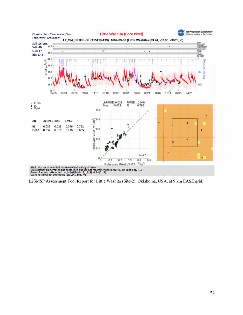
The key tool used in L2SMSP analyses is the chart illustrated in Figures 8.4.1 – 8.4.21. The charts show the comparison of the upscaled in situ soil moisture observations with the coinciding soil moisture retrievals. These charts include a time series plot of upscaled in situ and retrieved soil moisture as well as flags that were triggered on a given day, an XY scatter plot of SMAP-Sentinel L2SMSP retrieved soil moisture compared to the average in situ soil moisture, and the quantitative statistical metrics. Each CVS/candidate site is carefully reviewed and discussed by the L2SMSP Team and Cal/Val Partners. Systematic differences and anomalies are identified for further investigation. All sites are then compiled to summarize the metrics and compute the overall performance.

27

Table 8.4.1. SMAP Cal/Val Partner sites providing in situ data for L2SMSP assessment.

Site Name Site PI Area Climate regime IGBP Land Cover

Walnut Gulch*# M. Cosh USA (Arizona) Arid Shrub open Reynolds Creek M. Cosh USA (Idaho) Arid Grasslands

Fort Cobb# M. Cosh USA (Oklahoma) Temperate Grasslands

Little Washita# M. Cosh USA (Oklahoma) Temperate Grasslands

South Fork# M. Cosh USA (Iowa) Cold Croplands

Little River M. Cosh USA (Georgia) Temperate Cropland/natural mosaic

TxSON*# T. Caldwell USA (Texas) Temperate Grasslands

Millbrook M. Temimi USA (New York) Cold Deciduous broadleaf Tonzi Ranch M. Moghaddam USA (California) Temperate Savannas

Kenaston# A. Berg Canada Cold Croplands

Carman H. McNairn Canada Cold Croplands

Monte Buey M. Thibeault Argentina Arid Croplands Bell Ville M. Thibeault Argentina Arid Croplands

REMEDHUS# J. Martinez Spain Temperate Croplands

Valencia* J. Martinez Spain Arid Shrub (open)

Twente Z. Su Holland Temperate Cropland/natural mosaic Kuwait H. Jassar Kuwait Temperate Barren/sparse

Niger T. Pellarin Niger Arid Grasslands

Benin T. Pellarin Benin Arid Savannas Naqu Z. Su Tibet Polar Grasslands

Maqu Z. Su Tibet Cold Grasslands

Ngari Z. Su Tibet Arid Barren/sparse MAHASRI JAXA Mongolia Cold Grasslands

Yanco*# J. Walker Australia Arid Croplands

Kyeamba J. Walker Australia Temperate Croplands *=CVS used in L2SMSP 3 km assessment, # = CVS used in L2SMSP 9 km assessment

Table 8.4.2, and Table 8.4.3 give the overall results for the Beta Release dataset. The tables are for CVS comparison at EASE grids of 3 km and 9 km. Only 8 sites qualify to become as CVS for the 3 km EASE grid. This is a severe limitation when only a handful of CVS sites are used for validating the L2SMSP product at 3 km resolution. More sites need to be prepared or explored to improve the robustness of CVS assessment at 3 km. However, 8 sites are now used for the Beta Release assessment and it does provide insight and a path forward for further improvement of the L2SMSP product on the 3 km EASE grid.

Another strategy was developed to overcome the limitation of L2SMSP at 3 km assessment due to a low number of CVS sites. This strategy involve validating the L2SMSP product at 9 km by aggregating all nine L2SMSP 3 km EASE grid cells within the 9 km EASE grid and use most of the CVS sites developed for the SMAP-only Active-Passive L2SMAP 9 km product. This approach optimizes the CVS site usage and has potential to evaluate the spatially upscaled L2SMSP product at 9 km.

The figures in Appendix B illustrate the CVS assessment at 3 km EASE grid resolutions. They correspond to the map of the sites in Appendix A. Appendix C contains the CVS assessment at 9 km EASE grid resolutions.

28

Table 8.4.2. SMAP-Sentinel L2SMSP Beta Release CVS Assessment at 3 km

ubRMSE (m3/m3) Bias (m3/m3) RMSE (m3/m3) R

Site name BL Opt-1 BL Opt-1 BL Opt-1 BL Opt-1

Walnut Gulch 0.053 0.055 0.073 0.070 0.091 0.089 0.767 0.770

TxSON 0.029 0.032 -0.028 -0.016 0.041 0.035 0.921 0.924

TxSON 0.032 0.029 -0.034 -0.018 0.047 0.034 0.836 0.901

South Fork 0.061 0.060 -0.079 -0.077 0.104 0.098 0.817 0.836

Kenaston 0.056 0.044 -0.092 -0.087 0.107 0.097 0.317 0.482

Valencia 0.034 0.033 0.013 -0.001 0.037 0.033 0.516 0.531

Yanco 0.064 0.060 -0.013 0.003 0.065 0.060 0.778 0.834

Yanco 0.066 0.059 0.059 0.060 0.088 0.084 0.918 0.929

Average 0.050 0.046 -0.010 -0.009 0.075 0.071 0.731 0.777

Averages are based on the values reported for each CVS

Table 8.4.3. SMAP-Sentinel L2SMSP Beta Release CVS Assessment at 9 km

ubRMSE (m3/m3) Bias (m3/m3) RMSE (m3/m3) R

Site name BL Opt-1 BL Opt-1 BL Opt-1 BL Opt-1

Walnut Gulch 0.034 0.032 0.052 0.050 0.062 0.062 0.896 0.896

TxSON 0.021 0.024 0.017 0.003 0.027 0.024 0.914 0.912

TxSON 0.028 0.029 0.000 -0.001 0.028 0.029 0.946 0.955

Fort Cobb 0.029 0.029 -0.051 -0.048 0.058 0.056 0.885 0.886

Fort Cobb 0.034 0.034 -0.039 -0.038 0.051 0.051 0.761 0.750

Little Washita 0.041 0.037 -0.058 -0.061 0.071 0.071 0.751 0.805

Little Washita 0.039 0.032 0.023 0.016 0.046 0.036 0.792 0.855

Little Washita 0.026 0.025 -0.024 -0.022 0.035 0.033 0.883 0.885

South Fork 0.076 0.071 -0.060 -0.056 0.097 0.091 0.716 0.0741

Kenaston 0.048 0.037 -0.050 -0.058 0.069 0.068 0.436 0.0581

Kenaston 0.035 0.026 -0.050 -0.068 0.061 0.073 0.714 0.774

Remedhus 0.045 0.046 0.103 0.090 0.113 0.101 0.878 0.877

Yanco 0.052 0.050 0.025 0.034 0.057 0.060 0.891 0.924

Average 0.039 0.036 -0.008 -0.012 0.059 0.058 0.804 0.833

Averages are based on the values reported for each CVS

The key results of this assessment are summarized in the results in Table 8.4.2, and Table 8.4.3 for the SMAP L2SMSP algorithms applied at 3 km and 9 km, respectively. Table 8.4.2 highlights the results for Baseline and Option-1 of L2SMSP at 3 km. Although the Baseline and Option-1 algorithms have comparable performance for all the metrics (ubRMSE, Bias, RMSE, and R-value), Option-1 (direct soil moisture disaggregation) has sightly better ubRMSE. The Baseline algorithm (brightness temperature

29

disaggregation and then soil moisture retrievals) can likely be further improved in the future by the inclusion of better high-resolution ancillary information/data (e.g., soil texture map, actual NDVI, and surface temperature data) and optimization of tau-omega parameters at 3 km resolution. This might help in reducing the high bias now observed for most of the CVS sites at 3 km. For the subsequent Validated Release, we expect to have more CVS at 3 km for a robust assessment.

Table 8.4.3 summarizes the alternative approach for assessing the L2SMSP at 9 km EASE grid by maximizing the use of available CVS at 9 km originally prepared for the L2SMAP product. The results from Table 8.4.3 are encouraging. Both the Baseline and Option-1 have similar performance and high R values. The Baseline algorithm has better bias and meets the L1 accuracy requirement of the SMAP mission previously applied to the SMAP L2SMAP product. It is expected that the performance of the Baseline algorithm at 3 km will improve further, consequently improving the statistics of the Baseline algorithm at 9 km.

Based upon the metrics and considerations discussed, it is recommended that the L2SMSP Baseline algorithm be carried forward for the Beta Release because it has reasonable ubRMSE, bias, and correlation (R) as compared to the Option-1 algorithm, with the high probability of further improvement of these statistics for the validated release next year.

8.5 Sparse Network Analysis

Another form of assessment besides the CVS is the use of the sparse soil moisture network available across the continental United States and around the world. Examples of sparse networks include the USDA Soil Climate Analysis Network (SCAN), the NOAA Climate Research Network (CRN), the Oklahoma Mesonet, Pampas, GPS, COSMOS, SMOSMania, and Mahasri. The density of soil moisture observations from these networks is low, usually resulting in one point per footprint. These sparse network soil moisture observations cannot be used for assessment without addressing two issues: verifying that they provide a reliable estimate of the 0-5 cm surface soil moisture layer and that the one measurement point is representative of the SMAP footprint or grid cell. A bias between the point-scale sparse network soil moisture observations and coarse-scale satellite retrievals is likely because of the different area of measurements they support.

Table 8.5.1 shows statistics of one-to-one comparison of L2SMSP at 3 km with the sparse network sites (e.g., SCAN, CRN, Oklahoma Mesonet). The ubRMSE is ~0.054 for the SMAP-Sentinel active-passive baseline algorithm. The relative performance of the algorithms based on ubRMSE of sparse network analysis is similar to that obtained from the CVS analysis. However, the sparse network values are higher for ubRMSE and bias and lower for R, which is expected due to the significant change in scale between a point and the grid-based coarser scale L2SMSP product. The baseline algorithm performance is still good and provides additional confidence in the previous conclusions based on the CVS. Table 8.5.1: Statistics of comparison between the L2SMSP 3 km soil moisture retrievals and sparse network observations from CONUS and around the world. BL is the baseline TB disaggregation algorithm, DSM is the disaggregated soil moisture algorithm (Option-1), and N is the number of sites of a particular landcover.

30

31

8.6 Summary

The L2SMSP product uses the Sentinel-1A/1B SAR data to disaggregate SMAP L-band radiometer measurements from the ~40 km (half-power or -3 [dB] definition) radiometer measurement to a 3 and 9 [km] gridded product. The C-band SAR data adds spatial information to the radiometer product. It also adds the noise associated with radar measurements (instrument noise, complex surface scattering, etc.). It is expected that the spatial features in the L2SMSP product to be at higher resolution than the SMAP Level 2 Soil Moisture Passive (L2SMP/L2SMP_E) product. But the temporal behavior is expected to be comparable between the two products. These differences in the expected temporal and spatial characteristics affects the assessments based on different ground-based data sources.

The assessment of the L2SMSP product for initial assessment was primarily done using comparison statistics and time series plots with high-resolution airborne-based L-band data, the SMAP CVS and the sparse soil moisture network data. Each of these assessment approaches has advantages as well as shortcomings.

The CVS are time-series of in situ stations within SMAP grids that have been spatially averaged. They thus have no information on the spatial patterns of surface soil moisture but should be robust indicators of the temporal changes in soil moisture. In this respect the CVS are not indicative of the spatial resolution advantages of L2SMSP. The temporal statistics should be equal but not appreciably worse when comparing L2SMP_E versus CVS match-up time series and comparing L2SMSP versus CVS match-up time-series.

The spatial resolution performance of the L2SMSP can only be assessed with more complete ground sampling which is possible only with airborne field campaigns. These experiments provide a unique opportunity to demonstrate the spatial resolution advantages of L2SMSP when compared to L2SMP-E. We use available airborne data sets in this assessment report. However airborne field campaigns are performed over short periods and sporadically. So comparisons of temporal statistics are not possible with these data sources for assessment.

For the Beta Release, the goal was to conduct a Stage 1 validation assessment based primarily on airborne data and CVS comparisons using metrics and time series plots. The comparison of L2SMSP disaggregated brightness temperature with the SMAPEx 2015 airborne data showed that the Sentinel data do provide valuable surface information that is critical for obtaining high-resolution brightness temperature. The CVS and the sparse network analyses indicated that the baseline algorithm has comparable unbiased root-mean-square-errors (ubRMSE), bias, and correlation R to the Option-1 algorithm and also has a chance of further improvement in performance statistics. Based on these results, it is recommended that the Baseline approach be used as the primary algorithm for the Beta Release. In the CVS analysis, the overall ubRMSE of the SMAP-Sentinel active-passive baseline algorithm at 9 km is 0.039 m3/m3, which is below the SMAP mission L1 accuracy requirement for the original SMAP active-passive 9-km product.

However, the science and application communities should take certain caveats into consideration before using the L2SMSP product. There is a tradeoff between adding spatial resolution with C-band SAR data and noise-levels. The L2SMSP high resolution (3 km) comes at a cost of degradation in temporal statistics of disaggregated brightness temperature and retrieved soil moisture. Whereas the more spatially-averaged L2SMP-E product may have less temporal noise and temporal uncertainty when compared to L2SMSP, the L2SMSP will have more spatial resolution in term of resolving sharp and large-contrast features below the radiometer resolution. The degradation in accuracies is mainly imparted due to: 1) difficulties in comprehensively characterizing the active radar signal interactions with land surface components, 2) the uncertainties in the active-passive algorithm parameters used in the

32

disaggregation of brightness temperature, and 3) the random errors and biases in the static and dynamic ancillary data used for soil moisture retrievals. The high resolution L2SMSP product captures the spatial details and patterns of soil moisture that are not present in the SMAP radiometer-only enhanced product (L2SMP_E). Therefore, those users of SMAP data who require more frequent revisit and temporal accuracy can use the L2SMP_E product (which is posted at 9 km), and those users who need high resolution soil moisture patterns and details with slightly degraded accuracy and less frequent revisit can use L2SMSP data (posted at 3 km) for their science studies and geophysical applications.

-

33

9 OUTLOOK AND PLAN BEYOND BETA RELEASE

Satellite passive microwave retrieval of soil moisture has been the subject of intensive study and assessment for approximately the past fifteen years. Over this time there have been improvements in the microwave instruments used, primarily in the availability of L-band sensors on orbit. The soil moisture retrievals from such radiometer have spatial resolution ranging from ~40-50 km.

The SMAP observatory was the first of its kind delivering coincident and collocated measurements using an L-band radar and an L-band radiometer. The SMAP radar stopped working on 7th July 2015, but the SMAP radiometer continues to provide high-quality brightness temperature data. The SMAP active-passive algorithm produced data for nearly ~85 days at 9 km resolution before the SMAP radar stopped functioning. However, the SMAP Active-Passive algorithm has potential to use other satellite radar observations. This provides a unique opportunity to obtain the status of geophysical information such as soil moisture at much higher spatial resolutions by incorporating the Sentinel SAR data in the SMAP active-passive algorithm. The higher resolution SMAP-Sentinel Active-Passive (L2SMSP) soil moisture retrievals require assessment in order to assess their accuracy and uncertainty. It is expected that there will always be heterogeneity within the satellite footprint that will influence the accuracy of the retrieved soil moisture as well as its assessment. As a result, one should not expect that the assessment metric ubRMSE will ever approach zero except in very homogeneous domains. Bias tends to be indicative of a systematic error, possibly related to algorithm parameterization and model structure. Quality data are needed to discover and address these systematic errors. Some issues that should be considered beyond the Beta Release include the following:

The Stage 2+ validated product. In a future release, we expect to improve the Baseline algorithm parameters and the tau-omega model parameters, ultimately improving the absolute RMSE, bias and unbiased RMSE. With this, the L2SMSP assessment should exceed Stage 2+.

Inclusion of high-resolution ancillary data. Most of the ancillary data except NDVI that are used in soil moisture retrievals have coarser resolution than 3 km. Bringing in new data with high-resolution and better quality will improve the L2SMSP Baseline soil moisture retrieval performance. The soil texture map is one such ancillary data set. A new soil texture database from Soil Grid 1 km (from ISRIC) will be explored in the future to be included in L2SMSP processing. Soil surface temperature data are another candidate that need improvement. The current surface temperature data are from GMAO and have a resolution of ~25 km. Finding a new dataset for surface temperature will also be explored.

Increasing the number of CVS. There are only a limited number of sites that qualify as CVS at 3 km. Efforts have to be made to increase the number of CVS. This is key for a more robust assessment at 3 km.

Evaluate the impacts of algorithm structure and components on retrieval. There are some aspects of soil moisture retrieval algorithms that are used because they facilitate operational soil moisture retrieval. One of these simplifying aspects is the use of the Fresnel equations that specify that conditions in the microwave contributing depth are uniform. While there is ample evidence that this is true in most cases, it should be recognized that this assumption is a potential source of error – some effort should be made to evaluate when and where it limits soil moisture retrieval accuracy. Another assumption is that a single dielectric mixing model applies under all conditions globally. Any of the commonly-used dielectric models is highly dependent on the robustness of the data set used in its development. The impact of this assumption on retrieval error needs further evaluation.

Use of retrieved Tau. For the Beta Release, the parameter set defined in the L2SMP ATBD was implemented for computing tau using the climatology of vegetation-water-content (VWC).

34

Using a retrieved tau or alternatively, the real-year VWC (based on real-year NDVI) instead of climatology may help reduce the high unbiased RMSE observed for some cropland regions. The tau and omega parameters may also be used on alternate algorithms which use both horizontal and vertical polarization to remove the need for reliance on NDVI data altogether.

A median filter is implemented in L2SMSP SAS to remove outliers in the Sentinel data that are mostly observed over urban areas and manmade structures. The Median Filter is fairly successful in removing most of the outliers in the Sentinel data and ultimately improves the quality of the L2SMSP soil moisture product at 3 km. However, the appropriate way to remove the outliers is while processing and aggregating the Sentinel data from very high-resolution (~20 meters) to 1 km EASE grid data that becomes the input to L2SMSP SAS. Various approaches to quality control will be explored in the future to remove the Sentinel data outliers that do not represent the surface conditions pertaining to soil moisture features and retrievals. It is expected that during the Validated Release of the L2SMSP product, the filtering and quality control of the Sentinel data will be done outside of L2SMSP SAS.

35

10 APPENDIX

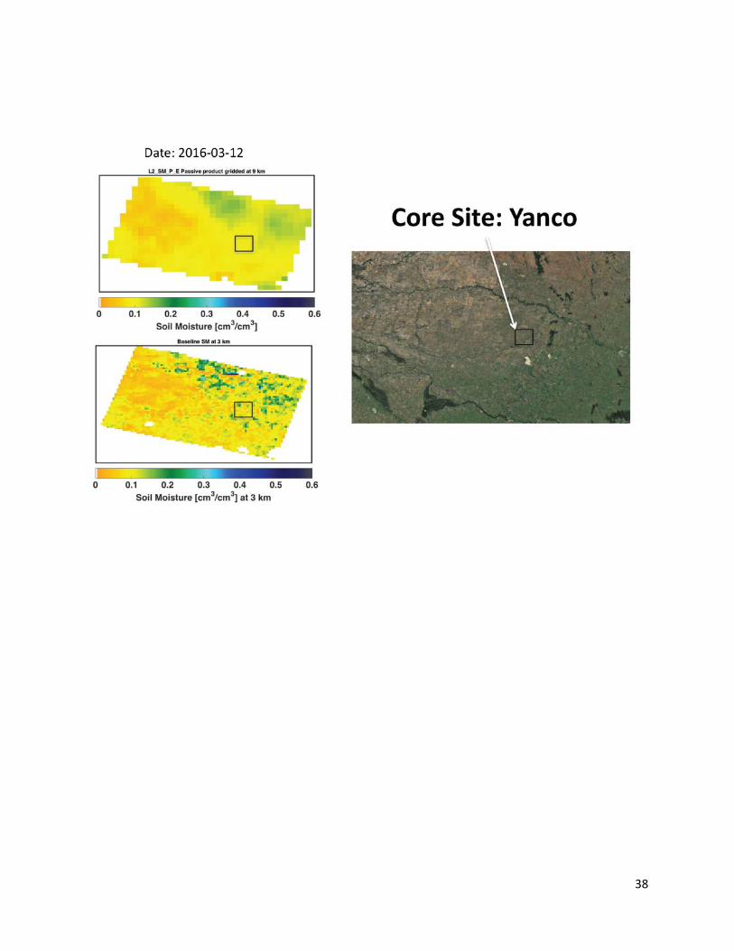
10.1 Appendix A: L2SMSP Maps Surrounding SMAP CVS

36

37

38

39

40

10.2 Appendix B: SMAP CVS Matchup Time Series at 3 [km] EASE Grid

L2SMSP Assessment Tool Report for Walnut Gulch, Arizona, USA, at 3 km EASE grid.

41

L2SMSP Assessment Tool Report for TxSON (Site-1), Texas, USA, at 3 km EASE grid.

42


43

L2SMSP Assessment Tool Report for Kenaston, Canada, at 3 km EASE grid.

44

L2SMSP Assessment Tool Report for South Fork, Iowa, USA, at 3 km EASE grid.

45

L2SMSP Assessment Tool Report for Valencia, Spain, at 3 km EASE grid.

46

L2SMSP Assessment Tool Report for Yanco (Site -1), Australia, at 3 km EASE grid.

47

L2SMSP Assessment Tool Report for Yanco (Site -1), Australia, at 3 km EASE grid.

48

10.3 Appendix C: SMAP CVS L2SMSP Matchup Time Series at 9 [km] EASE Grid

L2SMSP Assessment Tool Report for Walnut Gulch, Arizona, USA, at 9 km EASE grid.

49


50


51

L2SMSP Assessment Tool Report for Fort Cobb (Site-1), Oklahoma, USA, at 9 km EASE grid.

52

L2SMSP Assessment Tool Report for Fort Cobb (Site-2), Oklahoma, USA, at 9 km EASE grid.

53

L2SMSP Assessment Tool Report for Little Washita (Site-1), Oklahoma, USA, at 9 km EASE grid.

54


55


56

L2SMSP Assessment Tool Report for South Fork, Iowa, USA, at 9 km EASE grid.

57

L2SMSP Assessment Tool Report for Kenaston (Site-1), Canada, at 9 km EASE grid.

58

L2SMSP Assessment Tool Report for Kenaston (Site-2), Canada, at 9 km EASE grid.

59

L2SMSP Assessment Tool Report for Remedhus, Spain, at 9 km EASE grid.

60

L2SMSP Assessment Tool Report for Yanco, Australia, at 9 km EASE grid.

61

11 ACKNOWLEDGEMENTS

The research was carried out at the Jet Propulsion Laboratory, California Institute of Technology, under a contract with the National Aeronautics and Space Administration.

This document resulted from many hours of diligent analyses and constructive discussion among the L2SMSP Team, Cal/Val Partners, and other members of the SMAP Project Team. We acknowledge the collaboration of the Copernicus Sentinel Satellites Project. We also thank to the Copernicus Sentinel Satellites Project to accommodate the request of data acquisition of the Sentinel 1A/1B in SDV mode to cover most parts of the world. The authors of this report would like to express their gratitude for contributions by the following individuals, who collectively make this document an important milestone for the SMAP project: Jeffery Walker/University of Monash, Australia (for the SMAPEx data), the SMAP Algorithm Development Team, SMAP Science Team, and JPL Science Data System Team.

Acknowledgement for data: Sentinel-1A/B data are from the Copernicus Sentinel Satellites Project and processed by ESA.

62

12 REFERENCES

[1] Committee on Earth Observation Satellites (CEOS) Working Group on Calibration and Validation (WGCV): http://calvalportal.ceos.org/CalValPortal/welcome.do and WWW: Land Products Sub-Group of Committee on Earth Observation Satellites (CEOS) Working Group on Calibration and Validation (WGCV): http://lpvs.gsfc.nasa.gov.

[2] SMAP Level 1 Mission Requirements and Success Criteria. (Appendix O to the Earth Systematic Missions Program Plan: Program-Level Requirements on the Soil Moisture Active-Passive Project.). NASA Headquarters/Earth Science Division, Washington, DC, version 5, 2013.

[3] Dara et al., “Algorithm Theoretical Basis Document (ATBD): L2/3_SM_AP,” Initial Release, v.3, October 1, 2015. Available at http://smap.jpl.nasa.gov/science/dataproducts/ATBD/.

[4] Entekhabi, D., S. Yueh, P. O’Neill, K. Kellogg et al., SMAP Handbook, JPL Publication JPL 400-1567, Jet Propulsion Laboratory, Pasadena, California, 182 pages, July, 2014.

[5] Jagdhuber, T., M. Baur, M. Link, N. N. Das, and D. Entekhabi, Retrieval of active-passive microwave covariation Using the SMAP and Sentinel-1 data. IEEE Transactions on Geoscience and Remote Sensing, In Press.

[6] Das, N. N., D. Entekhabi, E. Njoku, J. Shi, J. Johnson, and A. Colliander, Tests of the SMAP combined radar and radiometer algorithm using airborne field campaign observations and simulated data, IEEE Transactions on Geoscience and Remote Sensing, vol. 52, pp. 2018–2028, 2014.

[7] Adams, J. R., McNairn, H., Berg, A. A., and Champagne, C. Evaluation of near-surface soil moisture data from an AAFC monitoring network in Manitoba, Canada: Implications for L-band satellite validation. Journal of Hydrology 521: 82-592, 2015.

[8] Ye, N., J. P. Walker, and C. Rudiger, A cumulative distribution function method for normalizing variable-angle microwave observations, IEEE Transactions on Geoscience and Remote Sensing, vol. 55, No. 7, pp. 3906–3916, 2015.

[9] Science Data Calibration and Validation Plan Release A, March 14, 2014 JPL D-52544.

[10] Chan S. K., Bindlish R., O’Neill P. E., Njoku E., Jackson T., Colliander A., Chen F., Burgin M., Dunbar S., Piepmeier J., Yueh S., Entekhabi D., Cosh M. H., Caldwell T., Walker J., Wu X., Berg A., Rowlandson T., Pacheco A., McNairn H., Thibeault M., Martínez-Fernández J., González-Zamora A., Seyfried M., Bosch D., Starks P., Goodrich D., Prueger J., Palecki M., Small E. E., Zreda M., Calvet J., Crow W. T., and Kerr Y., Assessment of the SMAP Passive Soil Moisture product, IEEE Transactions on Geoscience and Remote Sensing, DOI: 10.1109/TGRS.2016.2561938, 2016.

Documents

Soil Moisture Active Passive (SMAP) Project Assessment