1

SOIL MECHANICS SOIL MECHANICS

BASIC CONCEPTSBASIC CONCEPTS

1.1. PhysicalPhysical and index and index propertiesproperties of of soilssoils . . SoilSoil classificationsclassifications

2.2. Stresses in Stresses in soilssoils , , geostaticgeostatic stresses, stresses due to surface stresses, stresses due to surface loadsloads

3.3. Constitutive Constitutive lawslaws of of materialsmaterials

4.4. Water in Water in soilssoils

5.5. SoilSoil deformabilitydeformability and and soilsoil strengthstrength1.1. Consolidation and Consolidation and settlementsettlement of of soilssoils2.2. ShearShear strengthstrength . . BehaviourBehaviour of of sandysandy and and clayeyclayey soilssoils ..

Application to the case of the plane Application to the case of the plane failurefailure

SoilSoil mechanicsmechanics –– Basic conceptsBasic concepts

2

1.1. PhysicalPhysical and index and index propertiespropertiesof of soilssoils . .

SoilSoil classificationsclassifications

Physical properties of soils

• Definitions– Volumes

• V or Vt : Total volume of soil• Vs : Volume of solid grains• Vw : Volume of soil water • Va : Volume of soil air• Vv : Volume of voids (partly or totally filled with water)

– Weights• W ou Wt : Total weight of soil• Ws : Weight of solid grains• Ww : Weight of soil water• Wa : Weight of soil air (Wa = 0)

3

Schematic representation of soil, as a tree-phase med ium

Solid grains

air

water

WeightsVolumes

Wa = 0

Ww

Ws

Va

Vw

Vs

Phase diagram illustration of a soil that exhibits a total volume V and total weight WV = Vs + Vw + Va ; W = Ws + Ww + Wa

• Unit weights– Unit weight of grains: γs = Ws / Vs

– Unit weight of water: γw = Ww / Vw

– Unit weight of natural soil: γ = W / V– Unit weight of dry soil: γd = Ws / V– Unit weight of saturated soil: γsat = Wsat / Vsat

• Void ratio, porosity– Void ratio: e = Vv / Vs

– Relative density: Dr = (emax – e)/(emax – emin)– Porosity: n = Vv / Vt

– Effective porosity of saturated soil: ne = Vfree water / Vt

• Water content, saturation degree– Water content: w = Ww / Ws

– Water content of saturated soil: wsat = γw . Vv / Ws

– Saturation degree: S = Vw / Vv

4

Relationships between physical parameters

Solid grains

air

water

WeightsVolumes

Wa = 0

Ww = w. γs

Ws = γs

Va = (1 – S).e

Vw = S.e

Vs = 1

Vv = e

Phase diagram illustration with the hypothesis of Vs = 1 that allowseasily establishing relationships between physical parameters

Relationships between parameters(γs et γw being given)

� n = e / (1 + e)

� e = n / (1 - n)� γd = γs / (1 + e) = γs . (1 – n) � γ = γs . (1 + w) / (1 + e)

� w . γs = γw . S . e In case of a saturated soil, then: e ~ 2.7 . w

• Dry soil (w = 0, S = 0): one parameter among (γ = γd, γsat, e, n) is used to calculate the other parameters;

• Saturated soil (S = 1): one parameter among (γd, γ = γsat, e, n, w) is used to calculate the other parameters;

• Unsaturated soil: two independant parameters among (γd, γsat, e, n) and (γ, w, S) are used to calculate the other parameters.

5

Minerals and unit weights (kN.m -3)

23.0Attapulgite

27.5 – 27.8Montmorillonite

26.0 – 28.6Illite

25.5Halloysite (2H 2O)

25.5Kaolinite

26.2 – 26.6Serpentine

28.4Pyrophyllite

26.0 – 29.0Chlorite

28.0 – 32.0Biotite

27.0 – 31.0Muscovite

28.5Dolomite

27.2Calcite

26.2 – 27.6Na-Ca-Feldspath

25.4 – 25.7K-Feldspath

26.5Quartz

23.714.612460.140.85Silty sand and gravel

19.312.329550.401.20Micaceoussand

22.513.917490.200.95Fine to coarsesand

20.814.223470.300.90Silty sand

19.312.929520.401,10Uniform inorganic silt

19.313.529500.401.00Uniform clean sand

18.015.033440.500.80Ottawa standard sand

20.014.12647.60.350.92Uniform spheres

γdmaxγdminnminnmaxeminemax

Dry unit weightsPorosityVoid ratioDescription

Void ratios, porosities and dry unit weights of soils

6

Numerical values of phyisical parameters, after:

7

Cranularity – Granulometry – sedimentometryGrain size distribution curves

• Definition : Granularity is given by the distribution of grain weights as a function of size (width or equivalent diameter)

• Granulometry uses a sieve column for particle sizes more than 40µm or 80µm.

• Sedimentometry uses an hydrometer or a sedimentometer for particle sizes less than< 40µm or 80µm.

Granulometric curve

% in

wei

ghto

f tot

al s

oil

Particle diameters decreasing (logarithmic scale)

100%

0%

50%

(100 – y)% = retained on D y diameter sieve

y% = passing through the D y diameter sieve

y%

Dy

8

% in

wei

ghto

f tot

al s

oil

Particle diameters decreasing (logarithmic scale)

100%

0%

50%

y%

Dy

y’%

Dy’

This soil contains (y – y’) % in weight of total soil,made up of particles with diameters between Dy and Dy’ .

Well sorted soils or poorly graded soils

% in

wei

ghto

f tot

al s

oil

Particle diameters decreasing (logarithmic scale)

100%

0%

50%

y%

Dy

y’%

Dy’

This soil is well sorted or poorly graded. The grain size distribution curve is uniform.

This may be a sediment that has undergone a grain sorting:

� in the marine environment�Example: Fontainebleau sand, with Dy’ = 100µm and Dy = 300µm

� in the continental environment�Example: aeolian silt or loess, with Dy’ = 10µm and Dy = 50µm

9

Poorly sorted soils or well graded soils%

in w

eigh

tof t

otal

soi

l

Particle diameters decreasing (logarithmic scale)

100%

0%

y%

Dy

y’%

Dy’

This soil is poorly sorted or well graded. The soil exhibits a large range of particle diameters.

This may be a sediment that has undergone gravitational or fluvial transport, such as mountain screes or alluvial sands and gravels.

� Example: Screes, with Dy’ = 1mm and Dy = 50cm

� Example: Alluvium, with Dy’ = 100µm and Dy = 10cm

10

Granulometric indices

Fractiles: D25, D75, D50 = median value

Deciles: D10, D90

Uniformity coefficient: Cu = D60/D10Example: Cu<2: well sorted sands, uniform grain size curve

Sorting coefficient: S0 = D75/D25Example: S0<2.5: well sorted sediment (marine or aeolian sediment)

S0>4.5: poorly sorted sediment (gravitational, torrential, glacial sediment)

Coefficient of curvature: Cc = D302/(D60.D10)

Some of these indices are used for soil classifications

11

Sol 1: Gb, grave propre bien graduée, Cu = 30, Cc = 1,15Sol 2: Gm, grave propre mal graduée, Cu = 50, Cc = 0,25Sol 3: GL, grave limoneuse, WL = 45%, IP = 12%Sol 4: GA, grave argileuse, WL = 70%, IP = 40%

Sol 5: Sb, sable propre bien gradué, Cu=7,2, Cc= 1,14Sol 6: Sm, Sable propre mal gradué, Cu=2, Cc=1,0Sol 7: SL: sable limoneux, WL = 55%, IP = 22%Sol 8: SA, sable argileux, WL = 66%, IP = 37%

Soil 1: GW, clean well graded gravels, Cu = 30, Cc = 1,15Soil 2: GP, clean poorly graded gravels, Cu = 50, Cc = 0,25Soil 3: GM, silty gravels, WL = 45%, IP = 12%Soil 4: GC, clayey gravels, WL = 70%, IP = 40%

Soil 5: SW, clean well graded sands, Cu=7,2, Cc= 1,14Soil 6: SP, clean poorly graded sands, Cu=2, Cc=1,0Soil 7: SM: silty sands, WL = 55%, IP = 22%Soil 8: SC, clayey sands, WL = 66%, IP = 37%

12

Compactability of soils – Proctor curves

Normal Proctor Test and Modified Proctor Test

13

Caracterization of fine particles

Fine particles (<2µm) exhibit surface properties when in contact with water.These properties are named « activity » and can be described as cohesion, plasticity, shrinkage, swelling.

These properties result from:� the small size of clayey particles (<2µm, such as kaolinite, illite, smectite) and the corresponding

high external specific surface;� the crystal structure of phyllosilicates and the corresponding high internal specific structure,

especially for smectite, sepiolite, attapulgite;� the adsorption complex of clayey minerals with a general deficit of electric charges

and the possibility to adsorb dipolar water molecules and cations.

Kaolinite

Smectite7.2 Å

15 Å

General scheme of crystal structures of clayey mineral s

14

Activity of fine soils – Atterberg limits

Measurement of Liquid limit,using the Casagrande apparatus

15

Atterberg limits and indices

• Plasticity index: I P = wL - wP• 0 < IP < 5 Non-plastic soil• 5 < IP < 15 Moderately plastic soil• 15 < IP < 40 Plastic soil• IP > 40 Very plastic soil

• Consistency index: I c = (wL – w) / IP• Ic < 0 Soil with liquid consistence• 0 < Ic < 0,25 Soil with pasty or very soft consistence• 0,25 < Ic< 0,50 Soil with soft consistence• 0,50 < Ic< 0,75 Soil with firm consistence• 0,75 < Ic< 1 Soil with very firm consistence• Ic > 1 Soil with stiff consistence

• Skempton or activity index: A = I P / (%< 2µm)• A < 0,50 Soil with very low activity• 0,50 < A < 0,75 Soil with low activity• 0,75 < A < 1,25 Soil with medium activity• 1,25 < A < 2 Soil with high activity• A > 2 Soil with very high activity

Casagrande plasticity chart

A line

16

7.6120150270HAttapulgite

29.2223759Fe

28.7233154Mg

24.5112738Ca

25.3202949K

26.8213253NaKaolinite

15.36149110Fe

14.7494695Mg

16.85545100Ca

17.56060120K

15.46753120NaIllite

10.321575290Fe

14.735060410Mg

10.542981510Ca

9.356298660K

9.965654710NaMontmorillonite

ShrinkageLimit (%)

PlasticityIndex (%)

PlasticityLimit (%)

Liquid Limit(%)

Exchangeablecations

Mineral

Clayey minerals and Atterberg limits

17

N°200 sieve: 0.075 mmN°4 sieve: 4.75 mm

G: gravel, S: sand, M: silt, C: clay,O: organic soil, PT: peat, highly organic soilW: well graded, P: poorly gradedL: low plasticity, H: high plasticity

Soil classification

18

G: gravel, S: sand, M: silt, C: clay,O: organic soil, PT: peat, highly organic soilW: well graded, P: poorly gradedL: low plasticity, H: high plasticity

Engineering use chart

19

Approximate classification of cohesive soils and rocks

2. Stresses in 2. Stresses in soilssoils ,,

GeostaticGeostatic stresses,stresses,

Stresses due to surface Stresses due to surface loadsloads ,,

StrainsStrains in in soilssoils

20

Stress vector

Conventional notations

Stress tensor (1/2)

21

Stress tensor (2/2)

22

Mohr’s circle

23

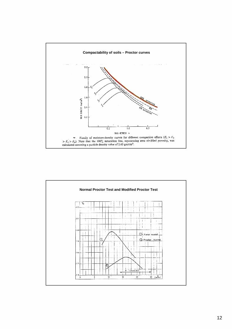
An exercise: calculation of the octaedral stresses

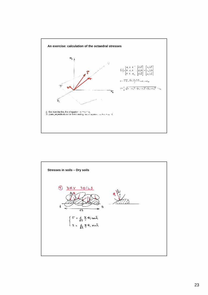
Stresses in soils – Dry soils

24

Stresses in soils – Saturated soils

Terzaghi’s equation

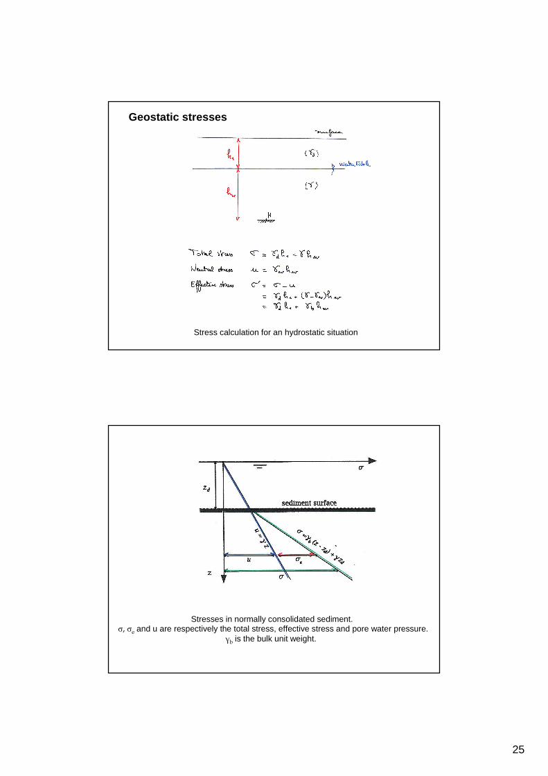
25

Stress calculation for an hydrostatic situation

Geostatic stresses

Stresses in normally consolidated sediment. �, �e and u are respectively the total stress, effective stress and pore water pressure.

γb is the bulk unit weight.

26

Pore water pressure forces acting on a submerged cylinder

Stresses due to surface loads

Stresses on elements due to concentrated load Q.(a) Rectangular coordinate notation. (b) Polar coordinate notation

27

Induced loads

Boussinesq Formula

Distribution of vertical stresses �z induced by point load Q. Dashed lines represent the �z distribution for various �z values at depth z.

Solid lines connect points of equal stress.

Bulbs of induced stresses

28

Example of approximate �z avg calculation on plane at depth z, using a simplified model

Geostatic stresses,stress increments,Stress path

29

Strain tensor (1/2)

Strain tensor (2/2)

30

3. Constitutive 3. Constitutive lawslaws of of materialsmaterials

Three fundamentalmechanical specific test:

�Loading test,

�Creep test,

�Stress relaxation test.

31

Perfectly elastic solid

Isotropic linear elasticity 1/2

h

∆h

S = π.r2

F

�1 = F/S �2 = �3 = 0

ε1 = ∆h/h ε2 = ε3 = ∆r/r

32

Isotropic linear elasticity 2/2

Viscous fluid/solid

33

Perfectly plastic solid and elasto-plastic solid

Elasto-plastic solid with hardening

ε

�

�1

�2

�3Failure

Plasticity thresholds

34

Examples of mechanical models of materials with different rheology:(a): ideal plastic (�0 = strength); (b): Bingham visco-plastic body;(c): Maxwell visco-elastic body; (d): Kelvin visco-elastic body

Examples of stress-strain diagramsfor different mechanical behaviours

Stress-strain diagram for an ideal plastic body

Stress plotted against rate of strain for a Bingham plastic body

35

Examples of strain-time diagramsfor different mechanical behaviours

Strain-time diagram for a Maxwell bodywhen the applied stress is held constant

Strain-time diagram for a Kelvin bodywhen the applied stress is held constant

Common types of stress-strain tests in laboratory

36

Oedometers

Triaxial apparatus

37

Direct shear box

4. Water in 4. Water in soilssoils

38

Water in soils 1/6

Water in soils 2/6

39

Water in soils 3/6

Water in soils 4/6

40

Water in soils 5/6

Water in soils 6/6

41

Seepage apparatus and test resultsillustrating Darcy’s law

Diagram of a typical setup for the field permeability test(after J.N. Cernica, 1995)

42

Example of calculation of the critical gradient

i = [(h + L + Z) – (L + Z)] / L = h/L

�’/L = γb – γw.h/L = γb – i.γw

�’ = 0 ↔ i = γb / γw

Example of pore water pressure calculation for an hydrodynamic case

43

Flow net for a thin cutoff wall

Flow net for steady-state flow through a homogeneous dam

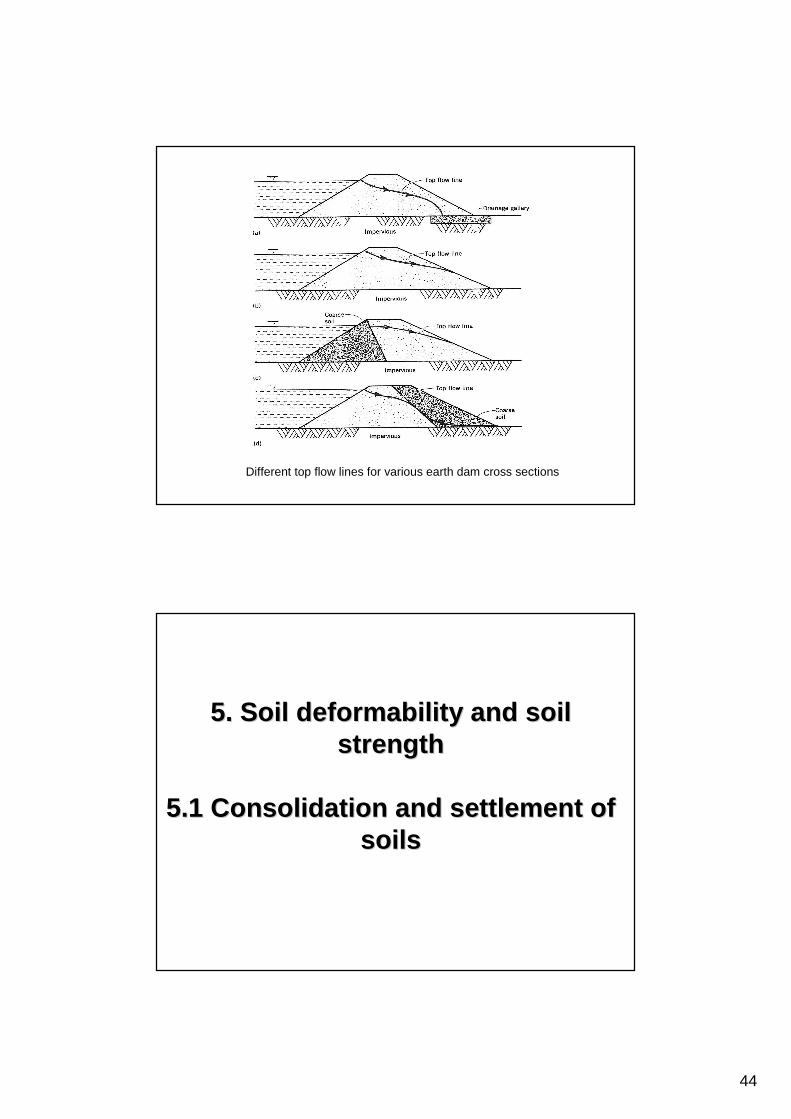
44

Different top flow lines for various earth dam cross sections

5. 5. SoilSoil deformabilitydeformability and and soilsoilstrengthstrength

5.1 Consolidation and 5.1 Consolidation and settlementsettlement of of soilssoils

45

Cross-section of a typical fixed-ring consolidometer

46

Unidimensional model of consolidation

0,1,2: the cell contains air = dry soil

3, 4: the cell contains water = saturated soil

1, 2, 3, 4, 5: the force F is applied

2, 4: the upper tap is open

5: the lower tap is open

(0)

Settlement curves:settlement w as a function of time t

Corresponding components used in the mechanical analogy model

47

Consolidation curve, for a given load �

The consolidation curve represents the void ratio as a function of timewhen a given load � is applied on the sample in the oedometer.

It allows to determine the amount of settlement for a given load �and the coefficient of consolidation Cv that accounts for the consolidation velocity

Oedometric curve

The oedometric curve results from the compilation of n (6 or 8) consolidation curves.

It allows to determine: the preconsolidation pressure Pc or �’c

and the compression index Cc.

48

Example of consolidation curves (arithmetic scale for time)

Determination of the theoretical 100% consolidation,the primary time effect and the secondary time effect

49

Determination of the coefficient Cα that accounts for the secondary compression

Schematic representation of the three usual components of settlement:1: immediate settlement

(different in the oedometer by comparaison to field conditions);2: primary consolidation (or Terzaghi consolidation);3: secondary compression (or secondary consolidation).

50

Example of experimental oedometric curves (pressure – void ratio curves)of an undisturbed precompressed clay soil.

(a): arithmetic scale; (b): logarithmic scale

Practical conditions for settlement calculations, usin g the oedometric curve

The amount of settlement

51

Principal causes of differential compaction or differential settlement

A: Difference in original thickness;

B: Difference in compactibility of mixed lithologies;

C: Differential compaction rates, in this caseproduced by a well, or well fieldlocated at the center of the illustration.

Original configuration is at left in each illustration, compacted configuration at right.

Compaction is to scale, with sand compacting from original porosity of 40 percent to a final 20 percent,clay from 80 percent to 20 percent.

C was assumed to be be precompacted, with initial sand porosity of 25 percent,initial clay porosity of 50 percent and final porosities as above.

52

Consolidation: Evolution of excess pore water pressures within a clayey layeras a function of time.Case of a compressible layer intercalated between two permeable layers

Consolidation ratio as a function of depth and time

The time dependent settlement

Average consolidation ratio: linear initial excess pore water pressure.(a) Graphical interpretation of average consolidation ratio U;(b) U versus T: time factor, U = F(T) = F(Tv) T = Tv = Cv t / H2

53

Average percent consolidation versus time factor U = F(T)

5. 5. SoilSoil deformabilitydeformability and and soilsoilstrengthstrength

5.2 5.2 ShearShear strengthstrength . . BehaviourBehaviour of of sandysandy and and clayeyclayey soilssoils ..

Application to the case of the plane Application to the case of the plane failurefailure

54

a) Ideal elasto-plastic materialb) Elasto-plastic material

Loose sand;Normally consolidated clay.

a) Elasto-plastic material with work softeningDense sand;Overconsolidated clay.

Examples of some elasto-plastic behaviours

55

Other examples of elasto-plastic behaviours

p = (�1 + �2)/2; q = (�1 - �2)/2

56

Unconfined compression testDefinition of cohesion C and internal friction angle φ

Envelope or intrinsic curve at failure

57

Mohr’s circles for various cases of stress

Results of direct shear test on sands

58

Shearing of a loose sand,with negative dilatancy or contractancy

Shearing of a dense sand,with positive dilatancy

Results of direct shear test on claysPeak shear strength and residual shear strength

59

Triaxial test – CD test

CD test1) Consolidated while �3 is applied2) Drained while (�1 - �3) is increasing until failure

Triaxial test – UU test

UU test1) Uconsolidated while �3 is applied2) Undrained while (�1 - �3) is increasing until failure

60

Triaxial test – CU test

CU test1) Consolidated while �3 is applied2) Undrained while (�1 - �3) is increasing, with measurement of u, until failure

Triaxial test – CU test

Measurement of Cu as a function of �1’