Evaluation of soil parameters.

By

Mr.Shashank Chakraborty

IIIrd year Department of Civil Engineering

Jalpaiguri Government Engineering College Jalpaiguri, West Bengal

Guided By

Dr.Biswajit Paul,

Environment science and Engineering,

Indian School of Mines, Dhanbad. Date: June-July, 2015

2

Table of Contents

Introduction 4

interpretation of parameters 13

Soil parameters 14

Experiment 22

Specific gravity 22

Porosity 23

Grain size analysis 24

Liquid limit plastic limit 28

Water content- dry density relation 33

Direct shear test 37

Conclusion 40

Bibliography 41

3

Acknowledgements

I would take this opportunity to thank the Principal, Jalpaiguri Government Engineering

College, Jalpaiguri (W.B) Professor J. Jhampati for providing me the opportunity to work

in this esteemed institution.

My, Head of the Department, department of Civil engineering, Professor Utpal Kumar

Mondol, for inspiring me to work in the field of engineering.

My guide, Dr. Biswajit Paul, Chair-professor, Department of Environment Science

Engineering, Indian school of mines, Dhanbad (Jharkhand) for his relentless help and

untiring support. His dedication and constant encouragement helped understand

intricacies of the subject.

My parents, their blessings help my fingers move.

Last but not the least, God Almighty.

4

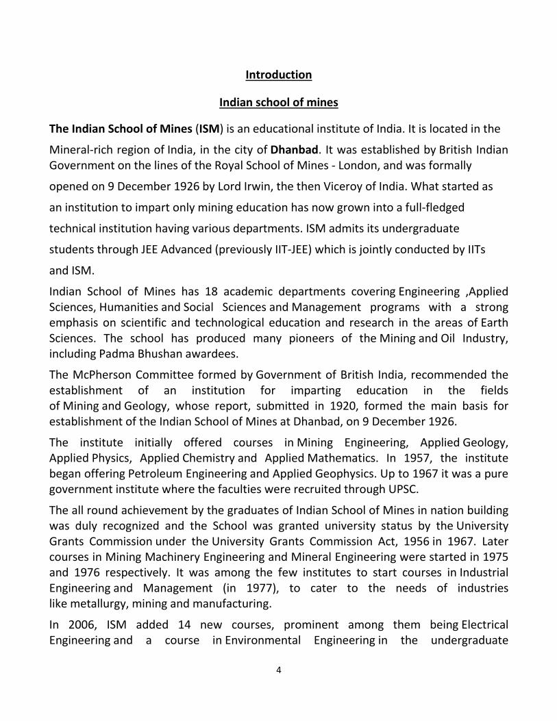
Introduction

Indian school of mines

The Indian School of Mines (ISM) is an educational institute of India. It is located in the

Mineral-rich region of India, in the city of Dhanbad. It was established by British Indian Government on the lines of the Royal School of Mines - London, and was formally

opened on 9 December 1926 by Lord Irwin, the then Viceroy of India. What started as

an institution to impart only mining education has now grown into a full-fledged

technical institution having various departments. ISM admits its undergraduate

students through JEE Advanced (previously IIT-JEE) which is jointly conducted by IITs

and ISM.

Indian School of Mines has 18 academic departments covering Engineering ,Applied Sciences, Humanities and Social Sciences and Management programs with a strong emphasis on scientific and technological education and research in the areas of Earth Sciences. The school has produced many pioneers of the Mining and Oil Industry, including Padma Bhushan awardees.

The McPherson Committee formed by Government of British India, recommended the establishment of an institution for imparting education in the fields of Mining and Geology, whose report, submitted in 1920, formed the main basis for establishment of the Indian School of Mines at Dhanbad, on 9 December 1926.

The institute initially offered courses in Mining Engineering, Applied Geology, Applied Physics, Applied Chemistry and Applied Mathematics. In 1957, the institute began offering Petroleum Engineering and Applied Geophysics. Up to 1967 it was a pure government institute where the faculties were recruited through UPSC.

The all round achievement by the graduates of Indian School of Mines in nation building was duly recognized and the School was granted university status by the University Grants Commission under the University Grants Commission Act, 1956 in 1967. Later courses in Mining Machinery Engineering and Mineral Engineering were started in 1975 and 1976 respectively. It was among the few institutes to start courses in Industrial Engineering and Management (in 1977), to cater to the needs of industries like metallurgy, mining and manufacturing.

In 2006, ISM added 14 new courses, prominent among them being Electrical Engineering and a course in Environmental Engineering in the undergraduate

5

curriculum. From 2006, ISM also started offering Integrated Master of Science (Int. M.Sc) in Applied Physics, Applied Chemistry and Mathematics & Computing, and Integrated Master of Science and Technology (Int. M.Sc Tech) courses for Applied Geology and Applied Geophysics. In 2011 ISM offered a B.Tech programme in Chemical Engineering. The institute introduced Civil Engineering in 2013 and Engineering Physics in 2014.

Departments and centres

ISM has the following Departments and Centres:

Engineering

Department of Chemical Engineering

Department of Civil Engineering

Department of Computer Science and Engineering

Department of Electrical Engineering

Department of Electronics Engineering

Department of Environmental Engineering

Department of Fuel and Mineral Engineering

Department of Mechanical Engineering

Department of Mining Engineering

Department of Mining Machinery Engineering

Department of Petroleum Engineering

Applied Sciences

Department of Applied Chemistry

Department of Applied Geology

Department of Applied Geophysics

Department of Applied Mathematics

Department of Applied Physics

Social Sciences

Department of Humanities and Social Science

Business

Department of Management Studies (Formerly Industrial Engineering & Management)

6

Centres

Centre of Mining Environment

Computer Centre

Center for Renewable Energy

Center of Societal Mission

Research Centers

An eight storey Central Research Facility is being set up at ISM as a Centre of National Importance. It is most likely to have an international accreditation.

Extension Centre in Kolkata

And an upcoming extension in New Delhi

An extension centre of ISM has been established in Salt Lake City, Kolkata, for promoting closer interaction with the industries.

CENTRE OF MINING ENVIRONMENT (CME): A Centre of Excellence of MOEF/ GOI

About the Center

A unique Centre of its kind ever since its establishment in 1987 under the sponsorship of

Ministry of Environment & Forests, Govt. of India, the Centre has been carrying out

advanced research in Environmental Science and Engineering with special emphasis on

Mining Environment.

The Centre has been conducting various types of Executive Development Programs

since its inception. The Centre has successfully completed two mega World Bank

assisted Projects on Environmental Capacity Building for Coal India Limited and also

build the capacity of Non- coal Mining Sector under World Bank assisted project of

Ministry of Environment and Forests /GOI.

The Centre has developed various modular Executive Development Programs on

Environmental Management in Mining Areas, Environmental Impact Assessment, Water

Management, Land Management, Air and Noise Pollution Management, Noise and

Human Response, Socio-economics and Mitigation and Social Impacts and

Environmental Legislation and its Implications, EIA & Auditing.

The Centre has organised over 100 training programmes with the training of over 1000

in-service personnel and other stakeholders and offers regular training of 1-2-4-6-13

7

weeks duration as per the requirements of the industry. The training program of 13

weeks duration has been recognized as fulfillment of requirement for environmental

cadre of its executives by CIL. The Centre is currently offering programmes as per the

requirement of the industry. It also offers consultancy services to the industry in the

areas of EIA, environmental management, environmental auditing, air and water

pollution control, wastewater management, reclamation of degraded lands, solid waste

management, noise abatement, etc.

The Centre has resulted Manuals, Books and Compilations, which serves the mineral

industry as reference material. The Centre’s Faculty won many laurels which include

National Mineral Award, Bala Tandan and M.L.Rungta Awards (MGMI & MEAI),

Institution of Engineer(s) Gold Medal, Subarna and Sashibhusan Memorial Award,

Bharat Jyoti Award, Michael Madhusudan Award, etc. The Centre assisted the

regulatory agencies (CPCB/MOEF) in developing environmental standards for coal

mining areas, guidelines for dust suppressant chemicals, mining in the forest land and

also preparation of operation Damodar Clean Action Plan. The Centre faculty served

various high level committees of Government of India including MOEF/GOI, BIS, DGMS,

MOC etc. Professor Gurdeep Singh is currently the Member Environmental Expert

Appraisal Committee (Mining) of MOEF/GOI.

ENVIS CENTRE

The Environmental Information System (ENVIS) at Centre of Mining Environment

(CME), Indian School of Mines (ISM), was established in 1991 by the Ministry of

Environment and Forests (MoEF), Government of India, for collection, storage,

retrieval and dissemination of information in the area of mining environment.

Our ENVIS Centre is accessible online since September 14, 2001 with a distinctive

website “http://www.geocities.com/envis_ism” which was launched by Shri

P.V.Jaykrishnan(IAS), Secretary to Government of India, MoEF. This website has

also been provided on NIC platform with a distinctive URL

“http://www.ismenvis.nic.in”.

The website has links to different organizations viz., different ENVIS Centres, Coal

& non-coal Organizations, Central Govt(Ministries) & Apex/Independent

organizations, Mineral rich States, Scientific Institutions, Universities, Organizations

related to Environment and Mining. Centre has provided variety of information in

the website viz., subject area, Best Practices Management, environmental

clearance related to mining, legislation, publications, database, experts, workshop

8

report, important Institutes, environmental awareness, research papers, research

projects, current events, current news, do you know section, equipments, photo

gallery, special lectures including Prof. S.K.Bose Memorial Lectures, query form,

feedback form, etc.

Centre also collected many Reports, Research articles, Proceedings and

Newsletters from various sources. All these hard documents are kept in the ENVIS

library for ready references.

Centre results publications on regular basis and till date 54 Newsletters, 14

Monographs, 9 Books have been published and 7 Compilations of Research

Publications of CME have also been made.

Department of Environment science and engineering

The Department of Environmental Science & Engineering is created out of existing

Centre of Mining Environment ( Established in 1987 as centre of excellence in the field

of mine environment by the Ministry of Environment and Forests, Govt. of India) at

Indian School of Mines in June 2007 with the commencement of a regular B.Tech

program in Environmental Engineering under IIT-JEE (first of its kind offered by any

national institute).

B.Tech. Environmental Engineering covering the following:

• Basic engineering and science subjects.

• Subjects on Air, Water and Soil Quality Monitoring, Assessment and Management,

Socio-economics, Environmental Legislation, EIA, Audit, Environmental Chemistry,

Environmental Ecology & Microbiology, Environmental Geotechnology, Wastewater

Engineering, Soil Mechanics, Fluid Mechanics & Hydraulics, Remote Sensing & GIS, etc.

• Environmental Leadership Projects.

• State of the art facilities for laboratory practical and hands on training.

• To cater the needs of industries: Chemical, Petroleum, Pulp & Paper, Textiles

Industries, Metallurgical, Mining and Allied Industries, Energy sectors, etc.

The Department also offers a regular M.Tech program in Environmental Science and

Engineering (since 1990) apart from Ph.D programs in Environmental Science and

Environmental Science and Engineering disciplines, respectively. It also offers a number

9

of courses at various levels in a number of B.Tech and M.Tech programmes of the

University. Well equipped laboratories and qualified faculty make it an ideal

Department for carrying out academic activities (Teaching, Research, HRD and

Consultancy). The Centre now functions within the Department of Environmental

Science & Engineering.

INFRASTRUCTURE

The Department has following well equipped laboratories for environmental

monitoring, assessment and pollution control:

LABORATORIES

Instrumentation Laboratory

Spectrophotometer (UV-VIS-IR, Shimadzu UV-256). Gas Chromatograph

AAS – GBC Avanta & GBC-902 including Graphite Furnace GBC GF 3000;

Mercury Analyser (MA 5800E)

Particle Size Analyser (CILAS/1064 liquid/dry, USA), laser based attached with

online image capturing facilities.

TCLP Apparatus including Zero Head Space Extractor, Dispensing Pressure Vessels,

Rotary Agitator & Vacuum Pressure Pump(Millipore)

Soil Quality & Soil Mechanics Laboratory

Field Kits for Water Holding Capacity, Infiltration Rate etc.

Sieve shaker, Muffle furnace;

pH & Conductivity Meters, Atterburg Limit Apparatus

Cone Penetrometer, Infra-red Moisture Meter

Triaxial Test Apparatus (AIMIL Digi Tritest), Permeameter (Falling & Constant head)

Consolidation Test Setup (AIMIL)

Hydrometer apparatus (SHIVALIK FHP motor)

CBR & Proctor Compaction Apparatus (Hydraulic and Engg. Instrument(HEICO))

Relative Density Apparatus,

Sedimentation Test Setup,

De-airing Apparatus (AIMIL).

Water Chemistry Laboratory

pH Meter with combined glass-calomel electrode (Cyber Scan 510, MEPC);

TDS/Conductivity Meter (Cyber Scan 200, MERCK);

Spectrophotometer (Spectroquant, NOVA 60, MERCK;

Flame Photometer (Microprocessor based, Model 128);

10

COD Meter (Spectroquant, TR 320 MERCK) (148°C);

Turbidity Meter (MERC, Turbiquant 3000T; 0-1000 NTU);

Immersion Thermostat (LAUDA, E100) – Bath/Circulation Thermostats

BOD Incubators;COD Reflux Units;Double Distillation Units.

Environmental Microbiology Lab

Continuous Weather Monitoring Station (Envirotech WM-300) – 1 no;

Mechanical Wind Recorder (Wilh Lambercht Gmbtt Gottingen Type-1482) – 3 nos;

Raingauge

Micrometeorological Lab

Universal Trinocular Research Microscope (OLYMPUS, BX60) – Digital Camera with

online image capturing & analysis, Micro Image lite 4.0

Trinocular Stereozoom Microscope (LEICA, 56D, 6.3:1) – Cold light illumination

system, Leica CLS 150 X

Millipore Membrane filtration for Coliform Organisms, Chlorophyl content meter

Colony Counter (Electronic); Laminar Flow Chamber (horizontal)

Leaf Area Meter (Systronics), Research Centrifuge (REMI R24)

Autoclave, ph & EC meter, Student Binocular Micrscope (NIKON) – 10Nos

Student Stereozoom Microscope – 10 Nos (LEICA)

Land Use & Hydrogeology Lab

Stereoscopic Microscope

Ground truth Radiometer

Optical Pentograph with 5x magnification, Clinometer, Rotameter

Liquid Permeameter (Ruska Haustan)

Electronic Digital Planimeter, Automatic Water Level Recorder.

AQUA CHEM and Aquifer Pro Software’s

Noise Quality Monitoring Lab

Modular Precision Sound Level Meter with octave filter set (Bruel & Kjaer)

Sound Level Meter (CRL-703A, Cirrus)

Modular Sound Analyzer (Bruel & Kjaer)

Noise Dose Meter (Bruel & Kjaer,)

Dosimeter (CEL 420), Audiometer (AP 251, Alfred Peters Ltd)

Radiation Lab

Alpha – Counter (Nucleonix, AP165)

Beta- Counter (Nucleonix, Minibin, MB 403)

Lead Chamber (Nucleonix, Minibin, MB 403)

11

Radon Bubblers (Polltech Instruments)

Radiation Survey Meter (Nucleonix, UR705)

Nal (T1) Detector (International Environment, 4K MCA with software 127A102/5A)

Radon Counter (Polltech Instruments, PS1-PCS1)

Lucas Cell (Polltech Instruments, PS1-RCD1)

Radioactive Standards (Nucleonix)

Fluid Mechanics Lab

Venturimeter, Orificemeter, Bernoullie’s Apparatus

Reynold’s Apparatus Pitot Tube, Display Model of Centrifugal Pump

Air Pollution Lab

High Volume Air Sampler & Respirable Dust Sampler (Envirotech)

Real Time Aerosol Monitor (RAM-1), Gravimetric Dust Sampler

Cascade Impacter (Sera Anderson), Fume Hood Chamber

Personal Dust Sampler (Envirotech), Stack Monitoring kit (Envirotech)

HVS Calibration kit (Envirotech)

Green House Gas Monitor , Portable CO Monitor (ENDEE)

Auto Exhaust Monitors for Diesel & Retrol Driven Vehicles (CO & HC)

Wastewater Engg. Lab

SBR, UASB, Hybrid and ASP Reactors,

Temperature Controlled Incubator cum Shaker

High Speed Refrigerated Centrifuge

Digesdhal Apparatus , COD Reactor, Stirrers

Soxhlet Extraction Assembly , Microprocessor based Muffle Furnace

UV-Visible Spectrophotometer , Gas Chromatograph &Vacuum Filtration Unit

Weather Station

The Department has an automatic weather station to provide the weather related

information (Max. Min. Temp, R.H, Wind Speed and Direction, Rainfall, etc.) to the

public on regular basis.

Land Surveying

Theodolite, Levels, Chain Survey Setup, Ranging rods, Plane Table Survey Setups,

Magnetic compass

Experimental Area

The Department is also equipped to carry out various studies on pilot scale levels

at the experimental plots for its transfer to real world situations.

Computer Laboratory

12

2 No. computer lab with 50 No’s of high end P- IV Computers with LAN & Internet

facility

Remote Sensing & GIS Lab

ERDAS 9.1, A0 Size HP T1100 Plotter, A0 Size HP 4500 Scanner, Recent & Archive

satellite data of different coalfields

The above laboratories are being further strengthened and modernized and a new

GIS/Remote Sensing Laboratory is being developed.

13

Interpretations of soil parameters.

Geotechnical engineering- an Introduction.

For some “soil” means just the top layer of soil, but for an engineer, soil means all

naturally occurring, relatively unconsolidated earth materials- organic or inorganic in

character-that lie above the bed rock. Now, soil can be broken into their constituent

particles relatively easily, such as by agitation in water. But rocks which are the source

of soils are an agglomeration of mineral particles bonded together by strong molecular

force. And this difference is not often clear. Hard soils can be termed as soft rocks or

vice versa.

Geotechnical engineering is a relatively new term which includes both rock and soil

mechanics and engineering portions.

History- During medieval times and even before that, humans had started using soil as a

construction material. There are many evidences of such structures in history. The

pyramids of Egypt, the famous Hanging Gardens built by Babylonian King

Nebuchadnezzar and the Great Wall of China. The Code of Hammurabi (2250 BC)

(Harper, R.F. (1904)) was one of the first attempts to codify building laws. In the Middle

Ages, the European engineers understood the problems associated with soil

settlements. The settlements of Leaning Tower of Pisa (Italy) and the Archbishop’s

Cathedral in Riga are well known examples.

It was early in the 18th century that the first attempts were made to develop some

theories regarding design of foundations and other constructions. Coulomb (1776), a

French scientist formulated classical theory on earth pressures. Concepts of frictional

resistance and cohesive resistance for soil bodies were introduced. Darcy’s law of

permeability and Stokes’ law of velocity of solid particles were developed in 1856.

Mohr’s rupture theory and Mohr’s stress circle developed in 1871 are extensively used

for analysis of shear strength of soils.

The beginning of 20th century witnessed some important developments related to

physical properties of soil. Atterberg (1911), defined consistency limits for cohesive

soils. Pioneering work in this field was done by the Swedish Geotechnical Commission of

the State Railways of Sweden. Though the progress was remarkable from 1900 to 1925.

14

This subject got a boost from its infancy only after 1925, due to the efforts of an

Austrian, Karl Terzhagi. The first publication on this subject was Terzhagi,

Erdbaumechanik (German; translates to soil mechanics in English). Other prominent

contributors were A. Casagrande, Taylor, Peck, Skempton et al.

During the Second World War, the air strips made on different soils possessing different

behavior led to a comprehensive study of soil and rock properties both physical and

chemical. Thus after the War the development of this subject was phenomenal. This fact

is documented in the International Conferences on Soil Mechanics and Foundations.

15

Soil parameters:

Specific gravity – Specific gravity of solids (Gs), is defined as the ratio of the weight of a

given volume of solid to the weight of an equivalent amount of water at 4ºC. Also be

defined as the ratio of the unit weight of solids to that of water.

The value of specific gravity is required in the determination of unit weight of solids,

unit weight of soil, void ratio, porosity, water content and other such parameters.

The value of Gs for majority of soils lies in the range of 2.65-2.80. Lower values are for

coarse grained sands. The presence of organic matter leads to very low values. Soils high

in metal or inorganic content (like mica or iron) return higher values.

Thus from specific gravity of a soil, one can guess up to a certain extent the type of

impurity present in the soil (like in case of higher values, heavy metals can be present,

which can cause ground water pollution or in case of low values, the soil might be high

in humus content). Moreover, void ratio and other important physical characteristics

required for calculation can be determined.

In order to measure the specific gravity of soil in laboratories, an apparatus called

Pycnometer is used.

Water Content- Direct or indirect measures of soil water are needed practically in every

kind of soil study. In the field, the knowledge of the water available for plant growth

requires a direct measure of some index of water content. In the laboratory,

determining and reporting many physical and chemical properties of soil requires the

knowledge of the water content of the soil. In soils work, water content has traditionally

being expressed as a ratio of the mass of water present in the sample to the mass of

sample after it has been dried to a constant weight. It is in fact a pure ratio.

To determine water content, the sample is dried. But a criterion must exist to determine

when a soil is ‘dry’. But in situations where precision or reproducibility is not required, a

precise definition of ‘dry’ is also not required. When high precision is a requirement

16

then a definition for ‘dry’ should exist followed by the method used for the

determination of water content of soil. Traditionally the most frequent definition of dry

being the constant weight of the soil after it has been dried in an oven at a temperature

of 100 -110 ºC.

If water content is desired on a volume basis, the volume from which sample is taken

must be known. A sampling device which takes a known volume of soil (Richard &

Stumpf, 1960) may be used; or the bulk density of the soil, as obtained from

independent masses in the same area.

Taylor (1955), working with Millville loam (which is a relatively uniform soil in so far as

physical and chemical properties are concerned), reported coefficients of variation of 17

and 20% for gravimetric measurements of water content of samples of soil from field

plots under irrigation by furrow and sprinkler methods, respectively. When water is

applied to soil by irrigation or rainfall, the quantity applied is reported as the depth of

water if it were accumulated in a layer. To obtain the volume of water applied to a given

area would require multiplication of the depth by the area, measured in the same

length units. In similar manner, the quantity of water in a soil profile may be reported as

the depth of water present if it were to be accumulated in a layer.

Direct methods are regarded as those methods wherein the water is removed from a

sample using evaporation, leaching or chemical reactions, with the amount removed

being determined. The key problem regarding water content determination in porous

materials has to do with the definition of ‘dry’ state.

Porosity- The structure of soil is related to many important soil physical properties

especially those pertaining to the retention and transport of solutions, gases and heat.

Soil structure can be measured in various ways, but perhaps it is most meaningfully

evaluated through some knowledge of the amount, size, configuration, or distribution of

soil pores. It is often the information concerning these pores, rather than particle size or

17

particle distribution which aids us in characterizing the soil as a medium for plant

growth or other use. Within the soil matrix there exists an array of complex

intraaggregate and interaggregate cavities which vary in amount, shape, size, tortuosity,

continuity. Precise quantification is not possible as their variation is large and nature

complicated. However, with the help of some assumptions, the size distribution of the

larger pores can be made with at least useful accuracy for both laboratories and field

purpose.

An important problem associated with characterization of pores is the unavailability of

standard terminology related to their classification into distinct size ranges. The need for

a standard classification scheme or index has been identified and various attempts

made. Cary and Hayden (1973), suggested the classification of micro-, meso- and

microporosity by Luxmoore (1981), and the responses of Bouma (1981), Beven (1981)

and Skopp (1981). Secondly, another problem arises, identifying pore sizes in terms of

cylindrical diameters. Commonly the equivalent diameters are measured with respect to

capillary pressure and liquid retention. Nitrogen sorption is an established practice for

determination of pore-sizes, but although widely used, method has limitations when it

comes to the wide range of pores that can be present in a sample. Wilkins et al. (1977)0

have described a procedure for direct measurement of soil pores larger than 20 μm by

vacuum impregnation with a fluorescent resin followed by sectioning and

photographing under black light.

The presence of pores in a soil gives an idea of it’s cohesiveness. A soil like clay will be

less porous and more cohesive whereas a soil like sand will be more porous and less

cohesive.

Particle size analysis- it is a measurement of the size distribution of individual particles

in a soil sample. The major features being destruction or dispersion of soil aggregates

into discrete units by chemical, mechanical, or ultrasonic means and the separation of

particles according to size limits by sieving and sedimentation. Soil particles cover an

extreme range of size, varying from stones and rocks to submicron clays. Various

18

systems of soil classifications have been used to define arbitrary limits and ranges of soil

particles.

Unified soil classification system (USCS), originally developed by Arthur Casagrande

(1948) was intended for airfield construction during the Second World War According to

this classification, coarse-grained soils are classified on the basis of their grain-size

distribution and fine grained soils classified on the basis of their plasticity.

AASHTO soil classification system was developed by the US Bureau of Public Roads was

developed, in the late twenties, a classification system called Public Roads

Administration which was specifically meant for road construction. The present AASHTO

(1978) is a revised version of the system in use in 1945.

Indian Standard Soil Classification System (ISSCS) was published in 1959 and revised in

1970. The revision is based on the USCS with the modifications that the fine grained

soils have been subdivided into three categories of low, medium and high

compressibility as against two in USCS.

Compaction- it is a process in which soil is restructured such that in theoretical language

one can say that there are no voids left in the soil. Practically this never happens. But

this process is utilized nonetheless, to improve the effort of soil as building material. The

soil gains get rearranged more closely, thus an increase in density is observed.

Compaction generally leads to increased shear strength values and helps improve

stability and bearing capacity of soil. Also reducing compressibility and permeability of

soil. Detrimental settlements, shrinkages can be avoided or controlled. Smooth wheel

rollers, pneumatic-tyred rollers, vibratory rollers etc. are most commonly used for field

compaction.

Usually the water content in a compacted soil is referenced as OMC. Thus, soils are said

to be compacted dry of optimum or wet of optimum. Permeability of a soil decreases

sharply with increase in water content on the dry of optimum. Minima occurs at or

slightly greater than the OMC. On the wet side of optimum it might show slight chances

19

of increase. The slight increase in permeability is due to the affect of a decrease in the

dry unit weight which is more pronounced than effect of improved orientation.

During compaction of man-made fills in layers, the soil below will be subjected to

normal and shear stresses. These induce pore water pressures. Soil compacted wet of

optimum will have higher pore water pressure compared to soils compacted dry of

optimum which have initially negative pore water pressure. (Punmia, 2001)

Atterberg limits- consistency is a term used to describe the degree of firmness of soil in

a qualitative manner using description such as soft medium, firm, stiff or hard. It

indicates the relative ease with which a soil can be deformed.

Depending on the water content, the four stages of consistency are used to define the

consistency of clayey soil: i) liquid state ii) plastic state iii) semi-solid state iv) solid state.

The boundary water contents at which the soil undergoes a change from one state to

another are called “consistency limits”. In 1911, Atterberg, a Swedish scientist, first

demonstrated the significance of these limits. They are also known as “Atterberg

Limits”.

When a fine grained soil is mixed with a large quantity of water, the resulting

suspension is in a liquid state, offering practically no resistance to the flow. Soil has

virtually no shear strength. If the water content is gradually reduced keeping the

consistency of the sample uniform, a stage comes when it starts offering resistance to

flow. This is the stage when the sample changes from possessing no shearing strength to

infinitesimal shear strength and changes from liquid to plastic state. The boundary

water content between the liquid state and the plastic state is called “liquid limit”.

If the water content is further reduced, the clay sample changes from the plastic state to

the semi-solid state at a boundary water condition called “plastic limit”. In a semi-solid

state, the soil doesn’t have plasticity; it becomes brittle. When pressure is applied, it

simply crumbles.

20

A further reduction in the water content, brings about a state when a decrease in

moisture, the volume of soil doesn’t change. The sample changes from semi-solid to

solid state. The boundary water content is called “shrinkage limit”. Below this the soil

begins to dry up and it is no longer fully saturated.

Shear strength of soil- Capacity of soil to resist shear stress. It is defined as the

maximum value of shear stress that can be mobilized within a soil mass. If this value is

equaled by the shear stress at any plane or surface, failure will occur in the soil because

of movement of a portion of the soil mass along that plane or surface. The soil is then

said to have failed in shear.

Slopes of all kinds, hills, mountains, embankments etc. remain stable only if the shear

strength of the composite material is adequate, otherwise failure takes place.

All stability analysis which normally use the limiting equilibrium approach, require the

determination of limiting shearing resistance. The shear strength is not merely a

property of the material but also a function of magnitude as well as manner of

application of load. Besides, the previous stress history of a natural soil deposit is also a

very significant factor in influencing its shear strength.

21

Experiments

Specific gravity

(IS 2720: Part III : Sec 1&2 :1980)

Aim- To determine specific gravity of soil.

Apparatus-

1. Pycnometer

2. Mixing tub and IS sieves 4.75mm

3. Balance –accurate to 0.01 g

4. Mechanical shaker

Procedure –

1. A sample weighing 200g in case of fine grained soils and 400g in case of coarse

grained soil needs to be prepared in accordance to the standard sample

preparation measures for disturbed soil. This sample should be oven dried and

then stored in an air tight container until required.

2. The weight of the gas jar and ground glass plate should be measured(to the

nearest 0.2g) , this is m1.

3. Approximately 200g of fine grained or coarse grained soil is to be introduced in

the jar and weighed (to the nearest 0.2g), this is m2.

4. Approximately 500ml of water is added within a temperature of ±2 ºC of the

average room temperature during the test.

5. Depending on the type of soil, for coarse grained soils the gas jar and contents

shall be set aside for a period of 4 hours. But for fine grained soil, the gas jar shall

be shaken by hand until the particles are in suspension and then placed in a

shaking apparatus and shaken for a period of 20-30 minutes.

6. Stopper of the jar is removed and inspected, in case of frothing, it is neutralized

by a fine spray of water and if some soil is stuck to the stopper it is washed clean.

Water is then added to within 2mm of the top.

7. Taking care not to trap air under the plate, the gas jar shall be dried carefully and

weighed(to the nearest 0.2g), this is m3.

22

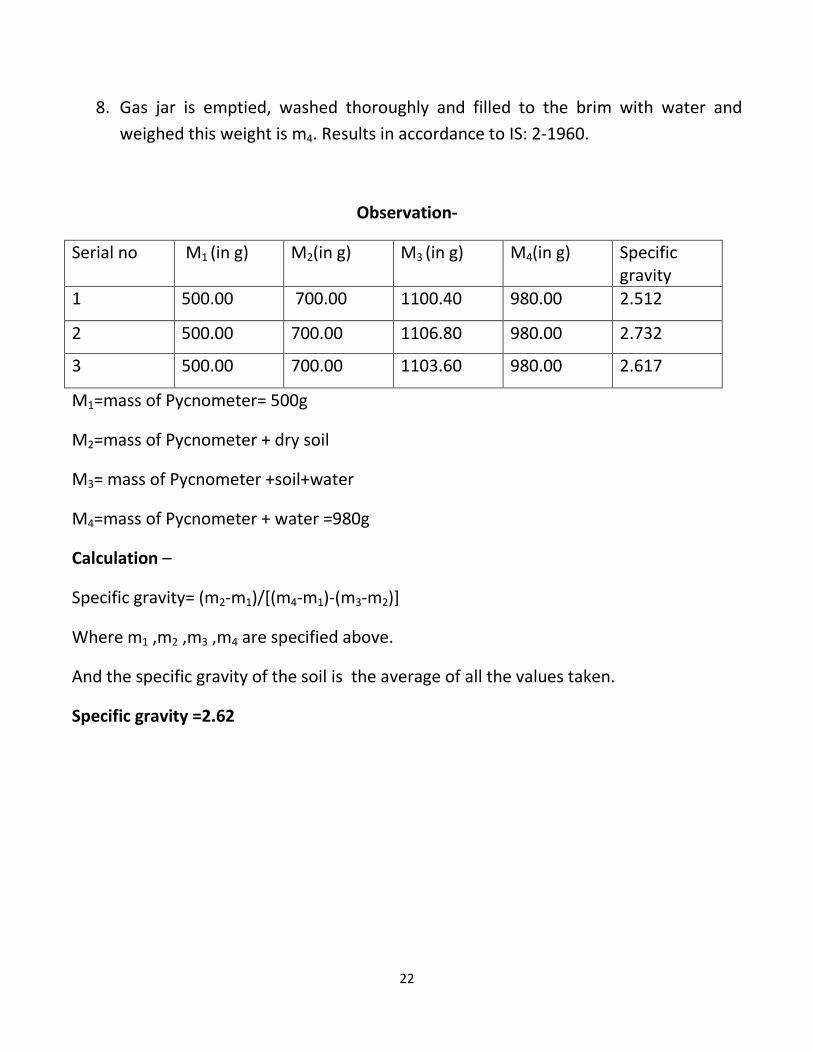
8. Gas jar is emptied, washed thoroughly and filled to the brim with water and

weighed this weight is m4. Results in accordance to IS: 2-1960.

Observation-

Serial no M1 (in g) M2(in g) M3 (in g) M4(in g) Specific gravity

1 500.00 700.00 1100.40 980.00 2.512

2 500.00 700.00 1106.80 980.00 2.732

3 500.00 700.00 1103.60 980.00 2.617

M1=mass of Pycnometer= 500g

M2=mass of Pycnometer + dry soil

M3= mass of Pycnometer +soil+water

M4=mass of Pycnometer + water =980g

Calculation –

Specific gravity= (m2-m1)/[(m4-m1)-(m3-m2)]

Where m1 ,m2 ,m3 ,m4 are specified above.

And the specific gravity of the soil is the average of all the values taken.

Specific gravity =2.62

23

Porosity test

Aim- To determine the void percentage or porosity of a soil.

Apparatus

1. Measuring cylinder.

2. Burette

3. Spatula

Procedure

1. An oven dried soil sample is placed in a measuring cylinder, it’s volume is

measured. This volume is Vs(volume of solid).

2. Distilled water is added to the sample by the means of a burette, drop by drop

until the soil is fully saturated or water starts accumulating over the top surface of

soil.

3. The volume of water used for this purpose is equal to the volume of voids (VV).

4. The process is repeated at least 3 times.

Calculations

The void percentage is calculated as,

e=(Vv/Vs)x100

Observation

Volume of solid (in ml)

Initial level in (ml)

Final level(in ml)

Difference(volume of water)

Void ratio e(%)

1 45 0 22.0 22.0 48.89 2 40 22.0 41.6 19.6 49

3 50 41.6 66.0 24.4 48.80

Void ratio is taken as the average of the 3 values, e =48.90

24

Grain size analysis

(IS 2720: Part IV : 1985)

Objectives

The purpose of this lab is to determine the grain size distribution and texture of an

unconsolidated sediment sample, using a standard sieve set, a Ro-tap automatic shaker

and graphical methods of data analysis. Definitions pertaining to IS 2809-1972 shall be

applicable.

Procedure

1. The sieves to be used are first measured and the weight recorded.

2. A kilogram of the soil sample is taken, sample should be oven-dried (at about 60

C) and free of large twigs, leaves or other organic debris. 25-30 grams of dried

sample is taken, the sample is carefully weighed, and the initial weight is

recorded. The sieve stack with largest mesh spacings on the top, progressively

smaller mesh spacings downward, and a pan on the bottom. Pour the sample in

the top sieve, Ro-tap for 20 minutes, and record the weight retained in each pan.

We will weigh by difference, so first record the weight of the weighing paper or

weighing tray. Then record the gross weight (weighing paper + sand retained)

and finally subtract the paper weight from the gross weight to obtain the net

sample weight retained. Results reported in accordance to IS: 2-1960.

3. Plotting the graph of the percentage soil retained versus the soil particle size

gives the detail of the type of soil. Actual range is given in IS: 1498-1970.

25

Observations

Sieve size (in mm)

Weight of sieve( in g)

Weight of sieve + soil (in g)

Soil retained (in g)

Cumulative weight(in g)

Percentage retained (%)

4.75mm 440 440 00 00 00 2mm 540 625 115 115 21.26

1mm 284 355 71 186 34.38

0.06mm 376 512 136 322 59.52 0.0425mm 257 331 74 396 73.12

0.0212mm 370 430 60 456 84.29 0.0150mm 225 280 55 511 94.45

0.0075mm 309 321 12 523 98.34 Pan 308 326 18 541 100

Calculations

Total weight retained=541 g

Difference between initial weight of sample and total weight retained: 1000-541=459 g

Note:

Gross weight = sieve weight + sample weight

Sieve weight = weight of the empty sieve

Net sample weight = gross weight – sieve weight

Total weight retained = sum of all individual sample weight

Individual weight percent = [(net sample weight)/ (total weight retained)] x 100

Cumulative weight percent = (sum of weights of all previous (larger) sand fractions)

+ (weight of current sand fraction)

26

Figure 1

Discussions

Engineering geologists and engineers use grain size analysis for site evaluations, building

and roadway construction, well construction and to evaluate slope stability. This is the

most common use of grain size analysis. These professionals use the d50 value as a quick

reference for grain size of a sample, and sometimes calculate the mean, median, mode,

sorting or skewness of a sample using the equations from the last section.

Other geologists have attempted to use grain size data to interpret the environment of

deposition for a sample. Some environmental interpretations are obvious: dunes and

beaches contain well sorted sediment, river sediment is moderately sorted, and glacial

sediment is poorly sorted. The problem with environmental interpretations is the

overlap between different environments. Many environments produce sediment with

similar textural properties.

4.75mm, 0

2mm, 21.26

1mm, 34.38

0.06mm, 59.52

0.0425mm, 73.12

0.0212mm, 84.29

0.0150mm, 94.450.0075mm, 98.34

Pan, 100

0

10

20

30

40

50

60

70

80

90

100

% retained

27

Sedimentary grains become more rounded as they move farther from the source, so

roundness may also provide environmental information. One complication with this

approach is that different minerals have different resistance to weathering. A quartz

grain may be transported 100’s or 1000’s of kilometers before it becomes rounded,

while a volcanic rock fragment may be rounded within a few kilometers.

28

Liquid limit and plastic limit test for soil

(IS 2720: Part V : 1985)

Aim – Determination of Atterberg Limits (liquid limit and plastic limit). Definitions

pertaining to IS: 2809-1972 shall be applicable.

Apparatus for liquid limit-

1. Casagrande’s apparatus or cone penetrator

2. Spatula

3. Grooving tool (Conforms to IS: 9259-1979)

4. Evaporating dish or petri dish

5. Oven

6. Balance

7. Distilled water

Procedure-

Soil sample preparation- As the sample taken is clayey(cohesive soil), it has been soaked

in water for a period not less than 24 hours before the test can be carried out. In case of

cohesion-less soil like sand, required water can be added such that the soil is in

suspension and the test can be carried out. (obtained in accordance to IS: 2720-1983)

The soil sample is to be remixed thoroughly before the test. A portion of the paste is to

be placed in the cup above the spot where the cup rests on the base, squeezed down

and spread into position with as few strokes as possible of the spatula and at the same

time trimmed to a depth of 1 centimeter at the point of maximum thickness, returning

excess soil to the dish.

A representative slice of the soil shall be taken in a container and it’s moisture content

expressed as a percentage of oven dry weight.

The cup is now fitted and dropped by turning the crank at a rate of 2 revolutions/second

until the two halves of the groove of the soil cake come in contact with bottom of the

groove along a distance of 12 millimeters. The length shall be measured with the means

of a grooving tool or ruler.

29

Now soil sample is to be tested, in each case the number of blows shall be recorded and

the moisture content determined by placing a nominal amount of sample in oven(which

is initially weighed) and the difference in the weights of the wet and the oven dried

sample gives the weight of water in that particular sample of soil.

The test should proceed from drier to wetter condition of the soil. The test may also be

conducted from wetter to drier condition provided drying is achieved by kneading of soil

and not by addition of dry soil.

WL , liquid limit of soil corresponding to 25 drops is taken.

Observations:

Water content, W is given by:

W=[(W2-W3)/(W3-W1)]*100

Soil sample no.

1 2 3 4 5

No of blows 17 21 25 28 32

W1(empty plate)(in g)

40.00 38.00 42.00 53.00 38.00

W2(empty plate +soil)(in g)

55.00 53.00 59.00 68.00 53.00

W3(oven dried soil)(in g)

52.34 49.63 54.21 64.12 50.46

W (water content)(in %)

21.17 28.97 40.95 34.89 19.04

WL=41% (rounded off to the nearest whole no.)

0

5

10

15

20

25

30

35

40

45

17 21

30

Figure 2

(rounded off to the nearest whole no.)

25 28 32

no of blows

water content

water content

31

Determination of plastic limit

Aim- To determine the plastic limit of a soil.

Apparatus- It shall conform to IS: 11196-1985.

1. Porcelain evaporating dish

2. Flat glass plate

3. Spatula

4. Palette knife

5. Surface for rolling

6. Air-tight containers

7. Balance

8. Thermostatically heated oven

9. Rod- 3mm in diameter and 10cm in length

Soil sample- Taking the soil earlier prepared for liquid limit test, the soil mass after

addition of water becomes plastic enough to be shaped into a ball.

Procedure-

1. After the soil is rolled into a ball, it is rolled between the fingers and the glass

plate with just sufficient pressure to roll the mass into a thread having a diameter

of 3mm.

2. The soil shall then be kneaded and rolled again. In order to measure if the thread

has a diameter of 3mm a rod having diameter 3mm is provided.

3. This process is continued until the soil can no longer be rolled into a thread, soil

crumbles before reaching a diameter of 3mm. This is considered a satisfactory

end point provided the soil has been rolled into a thread of 3mm in diameter

immediately before.

4. Care should be taken such that due to application of pressure, soil crumbles at

3mm diameter. Few pieces of crumbled soils are collected and their moisture

content determined. (according with IS: 2720 (Part 2)-1973)

32

Observations:

1 2 3 4 5

W1(in g) 40 38 42 53 38

W2(in g) 57 61 66 71 61

W3(in g) 52.33 56.32 60.34 67.47 57.14

W(%) 37.87 25.55 30.86 24.40 20.67

W1 weight of empty dish

W2 weight of dish + soil sample

W3 weight of dish + oven dry sample

Calculations:

Plastic limit WP=average of the water content=27.87%=28% (rounded to the nearest

whole no.)

Plasticity index (IP)= WL-WP= 41-28=13%

Flow index(IF)=( W1-W2)/log10(N2/N1)=7.75

Where W1 and W2 are water content corresponding to liquid limit and N1 and N2 are

corresponding drops.

If W1=21.17 W2=19.04 N1=17 N2=32

Toughness index (IT)=IP/IF =1.678

Liquidity index (IL)= (WO-WP)/IP =8%

Where WO is natural moisture content

WO=average of the water content obtained in liquid limit test=29.04

Consistency index (IC)=(WL-WO)/IP=0.996

33

Determination of water content-dry density relation using light compaction.

(IS 2720: Part VIII :1980)

Objective

To establish a relation between the dry density and water content. Also shows the

properties of soil as a construction material.

Apparatus- Definitions given in IS: 2809-1972 shall be applicable.

1. Cylindrical metal mould with base plate and collar- The cylindrical metal mould

has a diameter of 10 cm and height of 12.73 cm (measured by tape and slide

calipers).

2. Sample extruders

3. Balances-2 balances are required. One sensitive to 1g and other sensitive to

0.01g.

4. Oven- thermostatically heated oven.

5. Container – suitable non-corrodible air tight container to determine the water

content for tests conducted in the laboratory.

6. Steel-straightedge

7. Sieve -4.75mm and 20mm sieves as per IS requirements.

8. Mixing tools- pan, trowel, spatula etc.

9. Metal rammer having a weight of 2.5 kg. (conform to IS: 9198-1979)

Procedure

1. About 5 kg of sieved sample is obtained and weighed.

2. As the soil taken is clayey, distilled water equivalent to 8% of the mass is added to

the entire sample and mixed properly. Then the soil is stored in a air tight

container for a period of 24 hours.

3. The cylindrical mould with the base plate is weighed and its weight noted.

4. The sample is now filled to roughly one-third of the cylindrical mould fitted with

the metal collar, the metal rammer is used to compact the soil with 25 blows.

Care should be taken such that in each blow, the metal rammer is extended to the

full extent that is 31 cm.

34

5. After compacting the one third, sample is added to the cylindrical mould filling it

to two third of the mould. The soil is again compacted by 25 blows of the metal

hammer.

6. Further, soil is added to the mould. Care should be taken such that it does not

exceed the metal collar by 5 cm. This is again compacted by 25 blows of the metal

rammer.

7. After compaction is done, the collar is removed and the excess soil is removed

with the means of a metal straightedge. Then the mould with the soil is weighed.

Some soil sample is collected in a Petri dish (the empty weight is already

measured) and its weight measured. Then the Petri dish is kept in an oven at a

temperature of 110 ºC for a period of 24 hrs. Then its weight is measured and

water content determined. (as in IS: 2720-1973 Part II)

8. To the rest of the sample extra water equivalent to 3% of the soil mass is added

and the process is repeated.

9. In this way 5 readings are taken each having 3% more water than the previous

one.

10. The readings are recorded in the observation table.

Calculation

w=[(W2-W3]/(W3-W1)]x100

Volume of mould = πxD2xH/4=1000 ml

If D=10 cm and H=12.73 cm

Where, bulk density(ϒt ) and dry density (ϒd) is given by,

ϒt=W/V

ϒd=ϒt/(1+w)

Mass of mould is 5459 g or 5.459 kg

Mass of compacted soil= mass of (mould + soil) –mass of mould

35

Observation

Water content table:

1 2 3 4 5

W1 (in g) 40.00 38.00 42 53 38

W2 (in g) 55.00 53.00 57 68 53 W3 (in g) 53.88 51.73 55.52 66.31 51.91

w (in %) 8.10 9.25 10.91 12.65 14.35

Dry density-bulk density table:

1 2 3 4 5

Volume of mould (in ml)

1000 1000 1000 1000 1000

Mass of mould (in g)

5459 5459 5459 5459 5459

Mass of (mould +soil )(in g)

7375 7502 7617 7589 7505

Mass of compacted soil (in g)

1916 2043 2158 2130 2046

Bulk density ϒt (g/ml)

1.92 2.04 2.16 2.13 2.05

w (in %) 8.10 9.25 10.91 12.65 14.35

Dry density ϒd (g/ml)

1.78 1.87 1.94 1.89 1.79

36

Figure 3

Thus from Figure 3 it is clear that the optimum moisture content of the soil is

10.91% at a dry density of 1.94 g/ml.

Discussion

The importance of soil compaction can be understood from the fact that in modern

construction, concrete is widely and most commonly used. But this material has a

weakness, it is susceptible to damage from tensile forces. This happens when the soil

is not evenly compacted, thus swelling of soil occurs due to pore pressure and after

drying the soil settles again but due to this upheaval of soil, the concrete structures

develop cracks or can collapse. The most common example of improper soil

compaction being the Leaning Tower of Pisa, Italy.

1.78

1.87

1.94

1.89

1.79

1.7

1.75

1.8

1.85

1.9

1.95

2

8.1 9.25 10.91 12.65 14.35

w

a

t

e

r

c

o

n

t

e

n

t

(

%)

ϒd

37

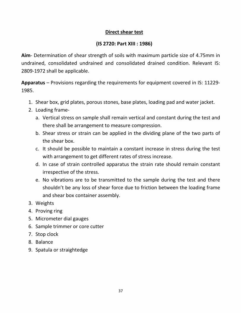
Direct shear test

(IS 2720: Part XIII : 1986)

Aim- Determination of shear strength of soils with maximum particle size of 4.75mm in

undrained, consolidated undrained and consolidated drained condition. Relevant IS:

2809-1972 shall be applicable.

Apparatus – Provisions regarding the requirements for equipment covered in IS: 11229-

1985.

1. Shear box, grid plates, porous stones, base plates, loading pad and water jacket.

2. Loading frame-

a. Vertical stress on sample shall remain vertical and constant during the test and

there shall be arrangement to measure compression.

b. Shear stress or strain can be applied in the dividing plane of the two parts of

the shear box.

c. It should be possible to maintain a constant increase in stress during the test

with arrangement to get different rates of stress increase.

d. In case of strain controlled apparatus the strain rate should remain constant

irrespective of the stress.

e. No vibrations are to be transmitted to the sample during the test and there

shouldn’t be any loss of shear force due to friction between the loading frame

and shear box container assembly.

3. Weights

4. Proving ring

5. Micrometer dial gauges

6. Sample trimmer or core cutter

7. Stop clock

8. Balance

9. Spatula or straightedge

38

Procedure

1. The soil specimen, sand in this case, is confined in a metal box of square

cross section that is split into two horizontal halves. The dimensions of the

box are to be measured.

2. As the sand specimen is dry, perforated plates are not required.

3. Porous stones are placed above and below the specimen which in turn is

placed between 2 metal grid plates.

4. Now the shear box or the metal box is placed in the trolley and the fixing

screws taken out.

5. A vertical load is applied, initially 0.5 kg/cm2, and the box is sheared

gradually.

6. The shear stress is measured by the micrometer dial gauge in the proving

ring, the shear is normally applied at a constant rate of strain.

7. The horizontal displacement is measured by means of another micrometer

gauge.

8. This process is carried repeated 2 times.

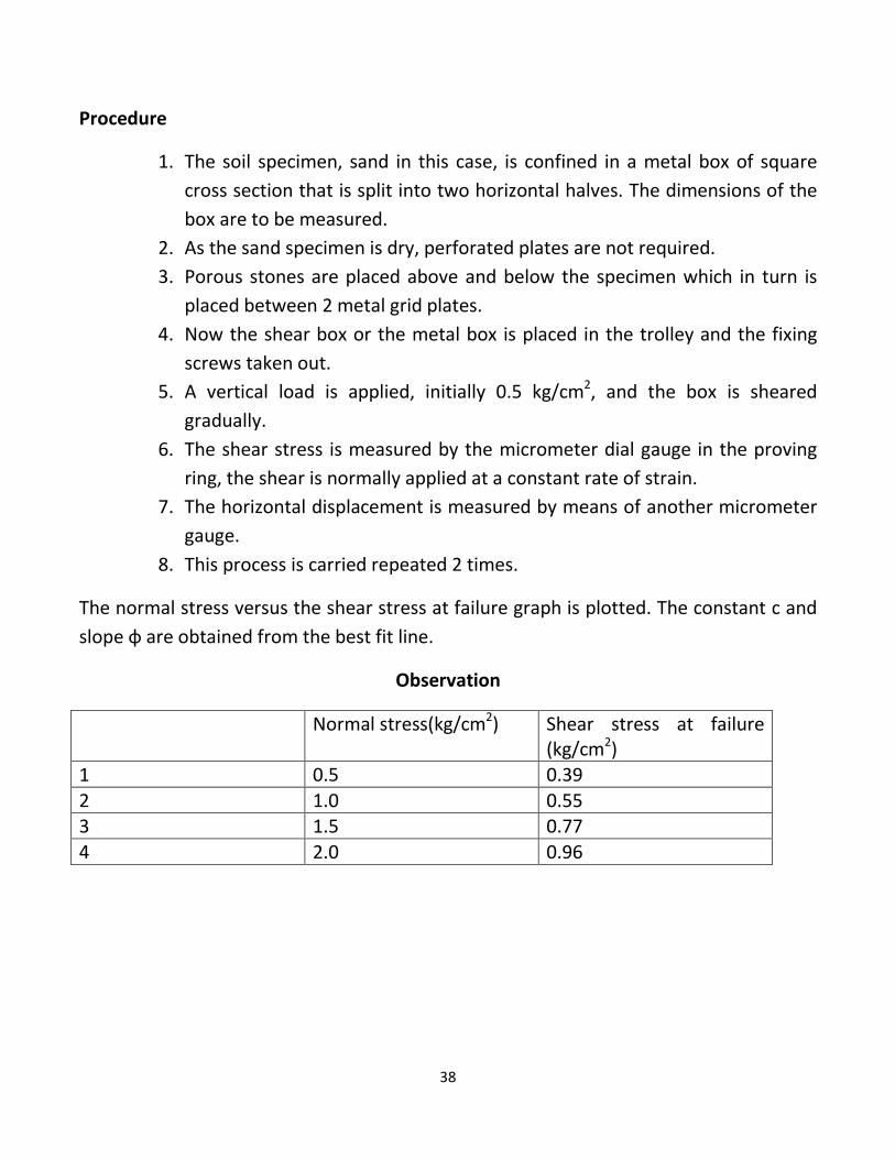
The normal stress versus the shear stress at failure graph is plotted. The constant c and

slope ɸ are obtained from the best fit line.

Observation

Normal stress(kg/cm2) Shear stress at failure (kg/cm2)

1 0.5 0.39

2 1.0 0.55 3 1.5 0.77

4 2.0 0.96

39

Figure 4

Thus from figure 4,

Value of c=0.14 kg/cm2

And ɸ=23º.

0

0.2

0.4

0.6

0.8

1

1.2

0.5 1 1.5 2

n

o

r

m

a

l

s

t

r

e

s

s

shear stress

shear stress

40

Conclusion

The soil taken for specific gravity test returned a specific gravity of 2.62 signifying

presence of organic matter. The soil sample taken is silty sand.

Taking the same soil sample, the porosity test is performed which returns a value of

48.90% of voids, thus the soil sample can be stated as porous. But porosity values of soil

like sands are even higher.

Grain size analysis is done on the sample and graphical interpretation leads to

concluding the soil as poorly graded sand.

The shear test performed on the sample gives us a constant c of 0.14, thus indicating the

soil to be sand with granules or some other impurities. The Mohr’s angle is 23º.

Thus the soil sample can be termed as poorly graded silty sand.

41

Bibliography

Atterberg, A. (1911),’Uber die physikalische Bodenunterasuchang, und uber die

Plastizitat der Tone’, Internationale Mitteilugen fur Bodenkunde, Verlag fur

Fachliteratur, Vol.1, Berlin, pp 301-310.

Coulomb, C.A. (1776),’Essai sur une Applications des Regles de Maximis et Minimis a

quelques Problems de Statique Relatifs a l’ Architecture’, Royal Academic des Sciences,

Vol. 7, Paris, pp 125-130.

Darcy, H. (1956), ‘Les Fountaines publiques de la ville de Dijon’, Paris, Victor Dalmount,

Editeur, pp 111-115.

Harper, R.F. (1904),’The Code of Hammurabi, King of Babylon, About 2550B.C.’, Chicago,

University Of Chicago Press, 2nd Edition, pp 90-112.

Lambe, T.W. and Whitman, R.V. (1969),’Soil Mechanics’, John Wiley and Sons, Inc., New

York, pp 102-106.

Rankine, W.J.M. (1857),’On the stability of Loose Earth’, Phil. Trans Royal Soc., Vol. 147,

London.

Rao, A.S.R. and Ranjan, G. (2013),’Principles of soil mechanics’, pp- 80-157.

Terzaghi, K. (1925),’Erdbaumechanik auf Bodenphysikalischer Grundlage’, Leipzig and

Wein, Franz Delicke, pp 112-114.