Embed Size (px)
Citation preview

Manual Software for Design of
Wastewater Treatment Plants
© by BITControl

The information and data in this publication can be changed without preliminary notice by the publisher at any time.
No part of this publication may be copied, reproduced or transmitted for any pur-pose, in any form or by any means, regardless whether electronical or mechanical without the written permission of Aqua Office.
The present software was carefully designed and tested. Nevertheless we cannot guarantee it being completely error-free. Furthermore we stress that the responsibil-ity of the plant designer is not transferred on the program or programmer by using the AQUA DESIGNER Software for plant design.
在不提前通知客户的前提下本公司仍然享有对软件内数据和说明进行更改的权利。
没有BITControl公司的明确授权本软件的任何部分不得以任何目的任何方式进行复制
与转载。
本软件已进行了认真地设置与调试。然而我们不能完全保证本软件没有任何纰漏。此
外特别提示您,由于错误操作所造成的损失本公司不承担任何连带责任。
February 2010, All rights reserved
© BITControl GmbH, Arzfeld, Germany

PREFACE
Welcome to AQUA DESIGNER, the new efficient tool for the design of wastewater plants. This software offers extensive help to solve routine tasks quickly and relia-bly. It will, thus, leave you time to spend on the more conceptional and creative as-pects of your work.
All calculation routines and variations have been thoroughly verified to ensure en-dorsement of your chosen concepts. You will save unexpected meetings and un-necessary feedback questions.
The supplemental part of the program in the ‘Extras’ allows an economic compari-son of the choices. Furthermore, extensive information for the subsequent design phases are supplied to you.
You will come to realise how easily and quickly effects of design changes can be reviewed and how they affect different parameters, e.g. effect on the activated sludge and secondary treatment through correlated changes in dry matter concen-tration and choice of a phosphate precipitation. Within minutes you will be able to determine the most economic choice through mass evaluation and evaluation of operating expenses. Your contractors will be convinced by the efficient design.


Content - 1 -
CONTENT
PREFACE................................................................................................................1
CONTENT................................................................................................................1
INTRODUCTION......................................................................................................7
Why AQUA DESIGNER? .....................................................................................7
New in AQUA DESIGNER ...................................................................................7
New in AQUA DESIGNER 6.3..............................................................................8
What is included in the package?......................................................................9
System Requirements ........................................................................................9
Conventions ........................................................................................................9
Software Installation......................................................................................... 10
Starting AQUA DESIGNER................................................................................ 10
HANDLING ............................................................................................................ 12
Menu Bar ........................................................................................................... 12
Fields and Boxes .............................................................................................. 14
Keyboard Functions ......................................................................................... 16
FIRST STEPS ........................................................................................................ 17
Demo Mode ....................................................................................................... 17
Introduction....................................................................................................... 17
Calculation based on ATV A131....................................................................... 18
Process............................................................................................................ 19
Waste Water Load........................................................................................... 19
Secondary Sedimentation Tank ....................................................................... 21
Clarified Water Outflow.................................................................................... 22
Basic Data ....................................................................................................... 22
Multiple Lines................................................................................................... 24
Activated Sludge Tank..................................................................................... 25
Aeration ........................................................................................................... 26
Sludge Recirculation........................................................................................ 28
Save Data........................................................................................................ 29
Sludge Storage................................................................................................ 29
Design Assembly .............................................................................................. 31
DIMENSIONING .................................................................................................... 33
Introduction....................................................................................................... 33
Dimensioning Limits......................................................................................... 33

- 2 - AQUA DESIGNER
Theory ............................................................................................................... 34
Activated Sludge System................................................................................. 34
Loading and Sludge Age ................................................................................. 36
Decomposition of Organic Matter .................................................................... 36
Nitrogen Decomposition .................................................................................. 37
Phosphorus Decomposition............................................................................. 39
Handling............................................................................................................ 41
Title- and Menubar .......................................................................................... 41
Main Window................................................................................................... 41
Fields .............................................................................................................. 42
Forms.............................................................................................................. 43
Loading ............................................................................................................. 44
Input Options................................................................................................... 45
Specific Values................................................................................................ 45
Absolute Values .............................................................................................. 48
Internal Response ........................................................................................... 49
Industrial Loads............................................................................................... 52
Total Load ....................................................................................................... 52
Pre Sedimentation ............................................................................................ 53
Choosing an ATV-Guideline ............................................................................ 53
Clarification Method......................................................................................... 55
Only Carbon Degradation................................................................................ 55
Only Nitrification .............................................................................................. 56
Nitrification and Denitrification ......................................................................... 57
Simultaneous Aerobic Sludge Stabilization...................................................... 67
External C-Dosage .......................................................................................... 68
Basic Data ......................................................................................................... 81
Organic Load and Sludge Volume Index ......................................................... 81
MLSS-Concentration / Sludge Tank ................................................................ 83
MLSS-Concentration / Influent ........................................................................ 84
Sludge Age and Excess Sludge ...................................................................... 84
Sludge and Volume Load ................................................................................ 86
Activated Sludge Tank Volume Requirements ................................................ 87
Return Sludge Ratio ........................................................................................ 88
Nitrification ...................................................................................................... 89
Denitrification .................................................................................................. 89
Phosphate Removal ........................................................................................ 92

Content - 3 -
Total Waste Sludge Production ....................................................................... 96
BOD5-Degradation .......................................................................................... 97
University Algorythm ........................................................................................ 98
Scope .............................................................................................................. 99
Variation of Method.......................................................................................... 99
Inflow ............................................................................................................. 100
Outflow Requirements ................................................................................... 100
Calculative Algorythm .................................................................................... 101
Constant Values ............................................................................................ 106
Continuous Flowed ASS................................................................................. 108
Upstream Anaerobic Chamber....................................................................... 108
Upflow Aerobic Selector................................................................................. 110
Secondary Sedimentation Tank ..................................................................... 113
Clarified Water Outlet .................................................................................... 129
Activated Sludge Tank................................................................................... 131
Aeration ......................................................................................................... 141
Return Sludge Transport ............................................................................... 160
Membrane System .......................................................................................... 161
Activated Chamber ........................................................................................ 161
Membrane Dimensioning ............................................................................... 162
Sequencing Batch Reactor............................................................................. 163
Process and Operational Variations............................................................... 163
Cycle Period .................................................................................................. 164
Reactor Volume............................................................................................. 165
Completed Computation ................................................................................ 174
Grit Chamber Design ...................................................................................... 175
Dimensioning ................................................................................................. 175
Equipment ..................................................................................................... 181
DATABANK ......................................................................................................... 185
Pumps.............................................................................................................. 187
Mixer ................................................................................................................ 188
Blower.............................................................................................................. 189
MENU DOCUMENTATION .................................................................................. 191
Operation......................................................................................................... 191
Description ...................................................................................................... 192
Dimensioning .................................................................................................. 193
Scaled Drawing.............................................................................................. 194

- 4 - AQUA DESIGNER
Supplememtary Calculations......................................................................... 194
Operating Costs.............................................................................................. 196
Control Keys.................................................................................................. 196
Energy Costs................................................................................................. 196
Sludge Disposal ............................................................................................ 202
Personnel Costs............................................................................................ 204
Total Operation Costs ................................................................................... 205
Benefits from the Anaerobic Digestion .......................................................... 205
MENU EXTRAS................................................................................................... 206
Components ................................................................................................... 206
Sludge Treatment ........................................................................................... 206
Thickener ...................................................................................................... 206
Sludge Tank.................................................................................................. 207
Anaerobic Sludge Digestion .......................................................................... 209
Separate Aerobic Sludge Treatment ............................................................. 213
Load Variation ................................................................................................ 218
Sludge Balance............................................................................................... 219
Pipelines.......................................................................................................... 220
Oxygen Efficiency........................................................................................... 221
MENU DRAWING................................................................................................ 225
Drawings ......................................................................................................... 225
Fields ............................................................................................................ 227
Membrane Aeration System .......................................................................... 230
Control Picture .............................................................................................. 231
Output of Drawings ....................................................................................... 231
Mass Calculation ............................................................................................ 232
Bouyancy ........................................................................................................ 233
VERIFYING ......................................................................................................... 235
Secondary Sedimentation Tank..................................................................... 235
Calculation .................................................................................................... 235
Hints.............................................................................................................. 238
Activated Sludge Chamber ............................................................................ 239
Guideline ....................................................................................................... 240
Type of Tanks ............................................................................................... 240
Phosphate Removal ...................................................................................... 241
Aeration......................................................................................................... 241
MENU OPTIONS................................................................................................. 242

Content - 5 -
Language......................................................................................................... 242
Settings............................................................................................................ 242
Options .......................................................................................................... 242
Documentation............................................................................................... 248
Operation Costs............................................................................................. 248
Export to Word............................................................................................... 248
Message Window .......................................................................................... 249
Process............................................................................................................ 249
General Constants .......................................................................................... 250
Generell ......................................................................................................... 250
Nitrogen Balance ........................................................................................... 250
Sludge Treatment .......................................................................................... 251
Buildings / Equipment .................................................................................... 252
Precipitant...................................................................................................... 252
Constants COD ............................................................................................... 253
Constants Hochschulgruppe ......................................................................... 253
Details.............................................................................................................. 254
FORMULAIC SYMBOLS ..................................................................................... 256
LITERATURE....................................................................................................... 262
SERVICE ............................................................................................................. 274

Introduction - 7 -
INTRODUCTION
Why AQUA DESIGNER?
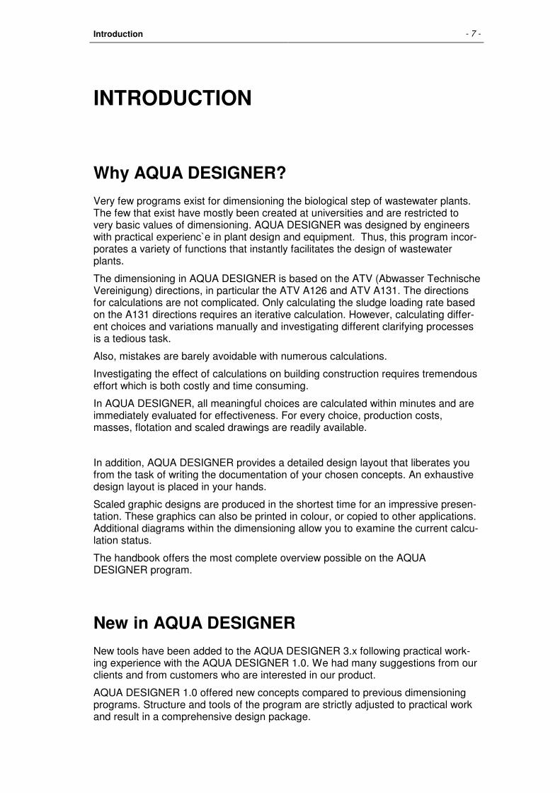
Very few programs exist for dimensioning the biological step of wastewater plants. The few that exist have mostly been created at universities and are restricted to very basic values of dimensioning. AQUA DESIGNER was designed by engineers with practical experienc`e in plant design and equipment. Thus, this program incor-porates a variety of functions that instantly facilitates the design of wastewater plants.
The dimensioning in AQUA DESIGNER is based on the ATV (Abwasser Technische Vereinigung) directions, in particular the ATV A126 and ATV A131. The directions for calculations are not complicated. Only calculating the sludge loading rate based on the A131 directions requires an iterative calculation. However, calculating differ-ent choices and variations manually and investigating different clarifying processes is a tedious task.
Also, mistakes are barely avoidable with numerous calculations.
Investigating the effect of calculations on building construction requires tremendous effort which is both costly and time consuming.
In AQUA DESIGNER, all meaningful choices are calculated within minutes and are immediately evaluated for effectiveness. For every choice, production costs, masses, flotation and scaled drawings are readily available.
In addition, AQUA DESIGNER provides a detailed design layout that liberates you from the task of writing the documentation of your chosen concepts. An exhaustive design layout is placed in your hands.
Scaled graphic designs are produced in the shortest time for an impressive presen-tation. These graphics can also be printed in colour, or copied to other applications. Additional diagrams within the dimensioning allow you to examine the current calcu-lation status.
The handbook offers the most complete overview possible on the AQUA DESIGNER program.
New in AQUA DESIGNER
New tools have been added to the AQUA DESIGNER 3.x following practical work-ing experience with the AQUA DESIGNER 1.0. We had many suggestions from our clients and from customers who are interested in our product.
AQUA DESIGNER 1.0 offered new concepts compared to previous dimensioning programs. Structure and tools of the program are strictly adjusted to practical work and result in a comprehensive design package.
- 8 - AQUA DESIGNER
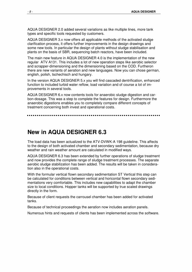
AQUA DESIGNER 2.0 added several variations as like multiple lines, more tank types and specific tools requested by customers.
AQUA DESIGNER 3.x now offers all applicable methods of the activated sludge clarification process, it offers further improvements in the design drawings and some new tools. In particular the design of plants without sludge stabilisation and plants on the basis of SBR, sequencing batch reactors, have been included.
The main new feature in AQUA DESIGNER 4.0 is the implementation of the new regular ATV A131. This includes a lot of new operation steps like aerobic selector and scrapper-dimensioning and the dimensioning based on the COD. Furtheron there are new variants of aeration and new languages. Now you can chose german, english, polish, tschechisch and hungary.
In the version AQUA DESIGNER 5.x you will find cascaded dentrification, enhanced function to included turbid water reflow, load variation and of course a lot of im-provements in several tools.
AQUA DESIGNER 6.x now contents tools for anaerobic sludge digestion and car-bon-dosage. This was a step to complete the features for design. Furthermore the anaerobic digestions enables you to completely compare different concepts of treatment concerning both invest and operational costs.
New in AQUA DESIGNER 6.3
The load data has been actualized to the ATV-DVWK-A 198 guideline. This affects to the design of both activated chamber and secondary sedimentation, because dry weather and rain weather amount are calculated in modified ways.
AQUA DESIGNER 6.3 has been extended by further operations of sludge treatment and now provides the complete range of sludge treatment processes. The separate aerobic sludge stabilization has been added. The results will be taken in considera-tion also in the operational costs.
With the formular vertical flown secondary sedimentation ST Vertical this step can be calculated for conditions between vertical and horicontal flown secondary sedi-mentations very comfortable. This includes new capabilities to adapt the chamber size to local conditions. Hopper tanks will be supported by true scaled drawings directly in the form.
Because of client requests the carrousel chamber has been added for activated tanks.
Because of technical proceedings the aeration now includes aeration panels.
Numerous hints and requests of clients has been implemented across the software.
Introduction - 9 -
What is included in the package?
The AQUA DESIGNER package consists of:
• AQUA DESIGNER program CD
• AQUA DESIGNER manuel
• Hardware keyfor a single-user version
This list of contents does not apply to the Demo-Version.
System Requirements
AQUA DESIGNER requires a PC with at least a Pentium processor, a minimum of 16 MB (32 MB recommended) memory and about 40 MB of hard disk space, that is compatible with indows 95, NT, XP or VISTA.
AQUA DESIGNER is a software working with a graphic user interface using win-dows features. This is why Windows must be installed on your computer prior to running AQUA DESIGNER.
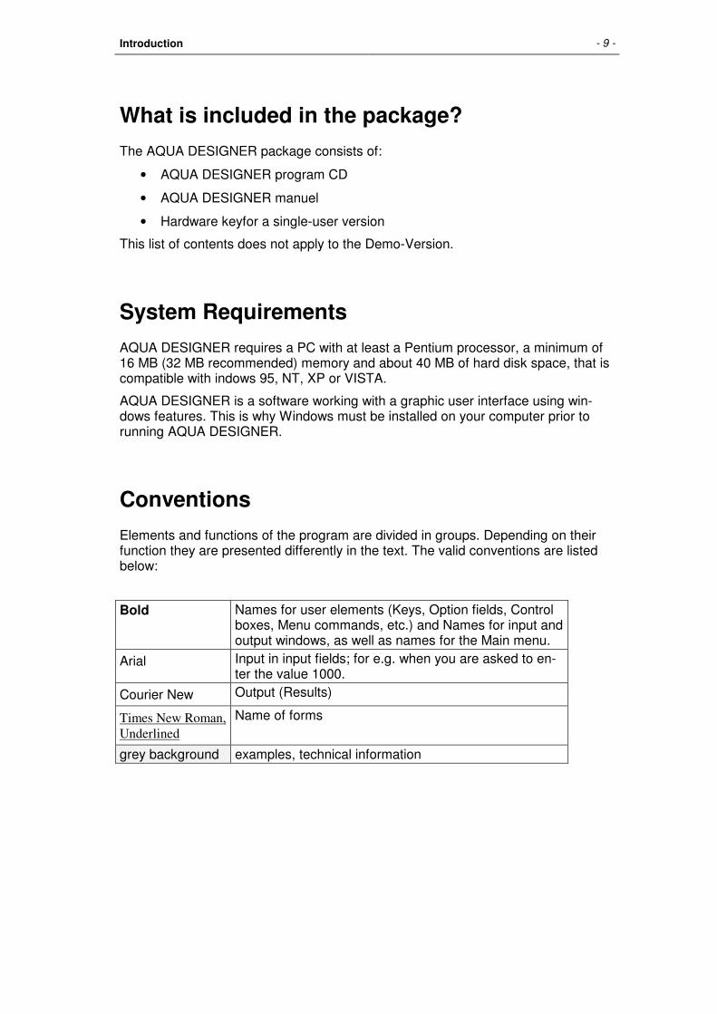
Conventions
Elements and functions of the program are divided in groups. Depending on their function they are presented differently in the text. The valid conventions are listed below:
Bold Names for user elements (Keys, Option fields, Control boxes, Menu commands, etc.) and Names for input and output windows, as well as names for the Main menu.
Arial Input in input fields; for e.g. when you are asked to en-ter the value 1000.
Courier New Output (Results)
Times New Roman,
Underlined
Name of forms
grey background examples, technical information

- 10 - AQUA DESIGNER
Software Installation
Is one of the above versions of Windows installed? If so, then you can begin to in-stall AQUA DESIGNER and the supplementary data files.
A special installation program that guides you through the installation process is included in the disk.
Installation with Autorun (Self Starting)
Insert the BITControl CD.
After the CD started, an installation window will occure.
Fig. 1: Autorun
Press Install AQUA DESIGNER.
Installation without Autorun (Start by Explorer)
Start the Explorer and go to the CD
In the directory “CD:\Aqua_Designer\installation” you will find the file “Setup.exe”. Start the file Setup.exe.
Problem Handling
If you get an error message concerning the MSVBVM60.DLL“, this means that this file is already existing on your system and just in use. Choose „Ignore“ and the in-stallation will continue.
If you received a demo version, the installation will be finished.
Starting AQUA DESIGNER
You can start AQUA DESIGNER in two different ways.

Introduction - 11 -
From the Start Menue
Click on Start > Programs > BITControl > AQUA DESIGNER.
Using Explorer
You can launch AQUA DESIGNER from the Explorer by double clicking on the file AD63.exe present in the application directory.
Copy Protection
AQUA DESIGNER is equipped with a dongle for copy protection. You have to plug it into an USB interface. If not, the software starts as a demo version.
Connect Files
With the file manager of MS windows you can connect the file typ *.AD1 with the software AD63.exe.

- 12 - AQUA DESIGNER
HANDLING
The Windows-Interface offers the possibility of working with either the mouse or the keyboard. The conventions for using the keyboard have been widely incorporated into AQUA DESIGNER.
Menu Bar
The menu bar contains almost all the required commands for operating AQUA DESIGNER.
Clicking on a menu, for example File, opens a menu window containing different commands. To operate one of the displayed commands simply click on it with the mouse.
Fig. 2: Menu File
The following table gives you an overview of the functions of the menu bar.
Menu Menu Commands Description
New To start a new project Open To open an existing project Save as To save a project under a new title Save To save a project Data Bank To save a project data in an access data
base Printer Properties To set the properties of the printer
File
Fonts The chosen typeface is not always available at the operating system. You can than choose another typeface and type size for operating surface, display and soft copy.

Handling - 13 -
List of recently opened files
Starting the programme for the very first time you must open the data through File-Open. After that you can open the recently used files directly from the list.
Exit To quit the programme. Eventually you will be asked, if you want to save the actual project.
Discription A description of the chosen methods and chosen machines. The description of every chosen vitalization method can be shown separately.
Dimensioning Accounting verification of the performed calculation, separate for each calculated method.
Calculation Grit Chamber
Accounting verification of the sand trap cal-culation
Operating Costs Calculation of electricity, sludge disposal, rotting means and staff costs, separate for each method
Short Documentation A summary of the most important calculated values on one page.
Documenta-tion
Results per Step Accounting verification of single modules A131, SBR,… A form to choose a vitalizing method Selection
Grit and Grease Chamber
A form to choose a sand and fat colleting method.
Thickener Design of the thickener Separate Aerobic Stabilisation
Design of the separate aerobic stabilisation
Anaerobic Sludge Degistion
Design of the anaerobic sludge degistion
Sludge Treatment
Sludge Tank Design of the sludge tank Drawings To go directly to the true scaled drwaing
function View Drawing To print or export (dxf) the drawing Mass Calculation To open the form for the mass calculation
with the drawing of the pit
Drawings
Bouancy To open the form for the bouancy Secondary Settling Tank
Recalculation of existing basin, determina-tion of a permitted hydraulic feed
Activated Chamber Recalculation of existing vitalizing sludge basin, determination of permitted freights
Verify
Aeration Determination of the aeration capacity of the permitted freights of an existing vitaliza-tion.

- 14 - AQUA DESIGNER
Components A choice of additional modules, which have an influence on the operating costs and the expositional report.
Sludge treatment Design of the sludge treatment: thickener, sludge tank, anaerobic sludge degistion with gas production
Loading Variation Variants of the calculation based on a per-formed and calculated method. Variation of temperature, pollution and dry matter concentration.
Sludge Removal Sludge balance for clearance basin down steam and return sludge flow suction sys-tem.
Pipelines Several important diameters of water, sludge and aeration pipelines.
Oxygen Efficiency Economic efficiency of the aeration system in kgO2/kWh.
Extras
Buffer Tank Calculation of the required volume of a buffer tank at SBR-constructions.
Language Choice of the operating and print out lan-guage
Settings Various settings for the calculation process, the complexity of the calculation, the scale and kind of prints outs.
Process Setting of the denitrification method, the aeration technique and several other vari-ants.
General Constants Parameters for various formulas, margin conditions and dimensions of constructions.
Constants COD Parameters for formulas of the dimension-ing based on COD
Options
Constants Hochschulgruppe
As mentioned above, constants for the commitment of the university group.
About AQUA DESIGNER
Version, licence, addresses
About BITControl Opens www.bitcontrol.info
Information
?
? Appeal to the off-line help, as F1
Fields and Boxes
Input Fields
Move the mouse pointer into an input field and double click on the field to mark the displayed value. An input entered via the keyboard overrides the displayed value.

Handling - 15 -
Leave the input field using the mouse or the keyboard. The last value typed in is then accepted.
Example The form Basic Data includes an Input field Sludge volume index. Move the mouse pointer into the white input field and double click. The value 100 or a value typed in before is marked in blue. Type a number of your choice with the keyboard overwriting the marked value.
Option Fields
Among different forms, you have the choice of selecting various options. In contrast to the control boxes you have to decide on selecting one option only. Upon opening a form, one option is always marked.
Fig. 3: Option Fields
Example In the form A126 Basic Data options for the organic load are shown. The option low is selected when the form is first opened. Clicking on the option high or high and varying, the program automatically calculates using the latest selected choice and the resulting effects.
Control Boxes
Clarifying processes or construction groups can be selected as additive modules. Marking the respective control box includes the selected module in the design.
Fig. 4: Control Box
Example
In Form A126 Basic data the control boxes for Denitrification and Phos-
phate Removal are included. Upon opening it for the first time, neither of the two boxes are checked. By clicking on them you mark and select deni-trification and/or phosphate removal.

- 16 - AQUA DESIGNER
Keyboard Functions
The operation elements can be called through the keyboard.
A few keyboard functions are listed below. All are in accordance with Windows stan-dard.
Function key
F10 The first menu on the menu bar is activated
Keyboard combinations
Ctrl + Esc Switches to another active Windows application
Alt + Tab Returns to the previously used application program
Alt + Print Screen Copies image of the active Window to the clipboard
Print Screen Copies the entire screen to the clipboard
Alt + Space bar Opens system menu
Alt + F4 Ends program
Alt The first menu in the menu bar is activated (in this case file)
As you can see from the list of keyboard functions, it is possible to simultaneously open other windows applications apart from AQUA DESIGNER. Thus, you can work in a word processing program or spreadsheet program at the same time. This can be very useful when you want to compare and check calculations performed in other programs with dimensioning in AQUA DESIGNER.

First Steps - 17 -
FIRST STEPS
Demo Mode
If a Demo Version is installed, the functions are limited. After starting AQUA DESIGNER a Demo Form occurs.
Fig. 5: Start Form
Here you are requested to choose your language.
After clicking on OK the Start-Windows of AQUA DESIGNER opens.
A new project will be started by File > New.
Please note, that in the Demo Mode its only possible to test AQUA DESIGNER with 5555 or 55555 inhabitants. That’s the limitation of the Demo Version.
Introduction
Using two examples presented below, you will be able to learn about the proce-dures involved in calculating the biological treatment step of a wastewater plant. Following this, you will assemble a plant design consisting of a detailed report, technical wastewater plant calculations and maintenance cost estimates.
After saving the project in a file, you will calculate the masses of concrete, steel and earth. With the chosen masses, you will evaluate the critical buoyancy factor of the pond(s). Finally, you will save the entire project.

- 18 - AQUA DESIGNER
In the first example, you will calculate a project using the ATV A126 guideline with-out considering options like denitrification, phosphate elimination or commercial wastewater volumes. In the second example, you will conduct a calculation in ac-cordance with the ATV A131. guideline. Here possible clarifying processes and other additional functions are considered.
Viewing and directly working on a completed project is possible by loading and us-ing one of the file examples from the Aqua_dir directory of AQUA DESIGNER. With File > Open you can load these files and continue the project with tasks like draw-ings or mass calculation.
Calculation based on ATV A131
To create or develop a new project, choose File > New on the menu bar.
The Main Window - the central operations interface - for the dimensioning appears. In this Main Window you will be guided through the calculations by coloured option fields.
Available options for all current calculation phases are distinguished by white back-grounds. If a calculation is actually performed, then the white background changes to a green background.
Unavailable fields have a grey background.
The control box Load has a white background at the beginning of the dimensioning process.
Fig. 6: First available step “Load” in the main window

First Steps - 19 -
Process
The kind of process is defined in the form Options > Process.
Fig. 7: Form Process for defining the kind of denitrification and the basis of calculaton
As standard, the intermittend denitrification is pre selected. If you start with File-New, the intermittend denitrification is automatically chosen.
Also in this example we will design a biological stage with intermittend denitrifica-tion.
Waste Water Load
Click on the field Load. This opens a form Waste Water Load. Here you will input the basic data for the wastewater plant load.
After leaving the field and clicking to another object, the specific wastewater amount will appear in the field Spec. Wasterwater Amount. Also the divisor of the daily peek occurs.

- 20 - AQUA DESIGNER
Fig. 8: Form Waste Water Load
Move the mouse pointer to the field marked Project and enter a project name.
With the mouse or tab key you can shift to the input field Population Equivalent. Enter 50000.
After leaving the field for Population Equivalent, by using the mouse or keyboard, the value 173 l/(Pxd) appears in the field Spec. Domestic Wastewater.
This is an ATV recommended value.
Also an hour index of 12, recommended by the ATV-DVWK A118 will be suggested.
Now use the mouse and go directly to Calculate. Next to the input field a window titled raw waste water appears. In this window Daily Charges (Loads) and Waste-water Volumes are displayed.
Clicking OK will take you out of the form Load and will take you back to the Main
Window.
In the Main Window the field for Basic Data based on the A131 guideline has a white background.
According to the ATV one can calculate in A126 or A131 choosing a population equivalent <= 5.000 inhabitants. As we had chosen 50,000 inhabitants, the A126 is not available for this example. With the new guideline A131 its also permitted to design small plants. So the A126 in practice is no longer in use.

First Steps - 21 -
Secondary Sedimentation Tank
In the Main Window you have the choice between a horizontal sedimentation tank and a vertical sedimentation tank as hopper tank or tank with flat floor.
In the Main Window choose the field ST horizontal (horizontal flown sedimentation tank) in the left part for A131.
This opens the form A 131 Sedimentation for horizontal flow.
Fig. 9: Form: Vertical flow secondary sedimentation tank based on ATV A126
In the left part you see the sludge properties. Here you can adapt the design to the sludge conditions of your project. The resulting diameter is 29.86 m. In practice tanks are built in steps of half a meter. So for practical demands its recommended to chose 30 meters as diameter.
Also in this example we reduced the diameter of the inflow building from 4.91 to 4.00 meters. We accept the displayed water level of 4.50 meters.
The secondary sedimentation tank is hereby calculated.
Now you can press the button Control picture to get a true scaled drawing ot the sedimentation tank. By clicking OK you will come back to the form of the secondary sedimentation.
Leave the form ST horizontal A131 by clicking on OK with the mouse.

- 22 - AQUA DESIGNER
Clarified Water Outflow
In the form Clear Water Outflow choose the option One sided overflow.
The limit for the hydraulic load of the one sided overflow weir is 10m3/(m*h). Click on Two sided overflow. You will get more distance to the limit of 6.00 m3/(m*h).
Fig. 10: Clear water outflow with two sided overflow weir
For smaller plants usually a one sided overflow is sufficient. For larger plants you have to change to two sided overflow.
Basic Data
Select Basic data for the calculation based on the ATV A131 guideline. Click on it with the mouse or move to it using the arrow keys on the keyboard.
The form A 131 Basic data appears.
The MLSS, mixed liquor suspended solids concentration, is a result of the calcu-lated sedimentation chamber. So its not recommended to take a higher value for this item.
At the top of the form you see, that we are calculating for simultaneous aerobic sludge stabilization in this example. So the biological part will be calculated based on a chosen sludge age of 25 days. This is the recommended minimum sludge age to get a stabilized surpluse sludge.
For phosphate elimination a simultaneous dosage of iron salt is chosen.
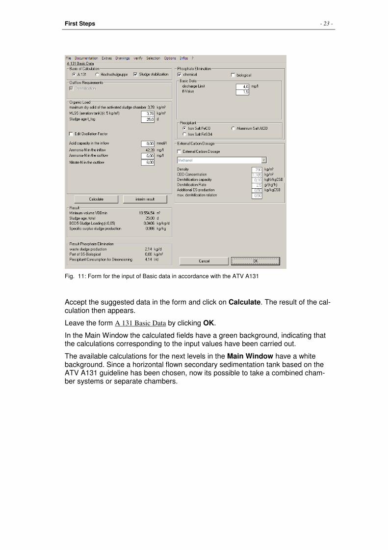
First Steps - 23 -
Fig. 11: Form for the input of Basic data in accordance with the ATV A131
Accept the suggested data in the form and click on Calculate. The result of the cal-culation then appears.
Leave the form A 131 Basic Data by clicking OK.
In the Main Window the calculated fields have a green background, indicating that the calculations corresponding to the input values have been carried out.
The available calculations for the next levels in the Main Window have a white background. Since a horizontal flown secondary sedimentation tank based on the ATV A131 guideline has been chosen, now its possible to take a combined cham-ber systems or separate chambers.

- 24 - AQUA DESIGNER
Fig. 12: Main window with calculated steps
Multiple Lines
In this example we will take two separate activated chambers. To take more than one line, we have to activate the multiple line property. In the menu bar under Op-tions > Settings, in the register Options, you can activate the multiline property.
Fig. 13: Activating the multiple line property with Options > Settings

First Steps - 25 -
Activated Sludge Tank
Select the field AT (ST extern).
ST extern signifies that the secondary sedimentation tank is a separate chamber.
Fig. 14: Activated sludge tank and secondary sedimentation tank as divided chamber system
Fig. 15: Activated sludge tank and secondary sedimentation tank as combined chamber system
The form A131 Activated Sludge Tank opens.
You can test different tank proportions by inputting various water levels.
Fig. 16: Calculation form for the activated sludge tank based on ATV A 131, as oxidation ditch, plug flow reactor

- 26 - AQUA DESIGNER
Choose a depth of 5 m and click on the field Calculate. In three steps you get the dimensions of an oxidation ditch. Take 22 for the width and 101 for the length.
Click on Control Graph. A scaled drawing of the selected tank is then displayed.
Leave the window by clicking on OK.
Aeration
Choose the field Aeration. A window Oxygen Transfer appears. Due to the se-lected calculation path, combined aeration and mixing is preselected.
You have the possibility to separately choose aeration and mixing. You can do this by selecting the option field Divided Mixing.
Fig. 17: Oxygen transfer with combined mixing and aeration
Accept the preselected values and click on Calculate.
The result of the calculation is displayed.
An additional window Blowers will automatically open to allow you to select com-pressors for providing compressed air.
A number of 4 blowers, as 2 blowers for each activated chamber is pre selected.
Click on the button Databank. This opens the window Blower Databank. The best matching blower from the databank will be suggested. You can find further informa-tion about the selection criteria in the chapter “Databank”.

First Steps - 27 -
Fig. 18: Selection of blowers
Click on Apply return to the form Aeration.
A window for the selection of mixers appears. Enter a number of 8 mixers. Click on Data Bank.
Slowe rotation mixers can be identified by the mixer diameter. Large diameters are corresponding with slow rotation. After selecting the mixers in the same way, you can design the aeration system.
Click on Membrane Aerator.
The standard suggestion for the aeration system is 8 lattices and 1 mixer per group. In this form usually its necessary to edit some values to get a good solution.
Example: Change the following fields: Mixer 1 Group to 2 Number Lattices to 14 Option: AERATION ONE SIDE Lattices Distance 1 m Tubular Aerators Load 6 m³/(mxh) Click the button Equipment and Change the value mixers – distance in front of mixers to 12 m.
Click on View Drawing after you have entered the above values. The drawings are displayed and updated. In a second window a single lattice is displayed and to its left detailed technical data of the pictured lattice and the aeration of the according chamber (tank) are listed.

- 28 - AQUA DESIGNER
Fig. 19: Form Membrane Aerator
Leave the Window Membrane Aeration with OK and select Return Sludge in the Main Window.
Sludge Recirculation
In the form Return Sludge Transport you have three options for the sludge transport.
Choose Centrifugal pump for the sludge conveyor. A window Centrifugal Pump then opens.
Fig. 1: Sludge transport with centrifugal pumps
Enter 2 into the input field for Number of Pumps and click on Data Bank.

First Steps - 29 -
Accept the recommended pump.
Leave the form Return Sludge Transport with OK.
Save Data
With this you have completed one calculation using the ATV Arbeitsblatt A131. This is visible by a continuous green line leading from Load up to Sludge Tank in the Main Window.
Fig. 20: Main Window with completed calculation
At this stage it is prudent to save the completed calculation to avoid losing data.
In the menu File choose the command Save as. The Standard-Windows menu ap-pears.
All AQUA DESIGNER data files are identified by the extension .AD1. Keep this ex-tension so that AQUA DESIGNER can automatically recognise the files.
Sludge Storage
You will find the sludge tank under Extras > Sludge Treatment > Sludge Tank.
In the form Sludge Tank enter the values as shown in the picture and click on Calcu-
late. The required volume of the container is displayed for the selected detention time and thickening.
Mark the control box for Mixer. This means that a mixer is selected to optimise the sludge thickening.
It is required to select the control box for Pump as well when there is no equipment for sludge removal available.

- 30 - AQUA DESIGNER
Fig. 21: Calculation form for sludge tank
Move the mouse to the input field Chosen Diameter and substitute the 7 with 14.
Click on Calculate. The required height appears.
In the window Mixer click on the button Data Bank and accept the recommended mixer by clicking on Take.
Click on OK to leave the form.
The documentation of the sludge tank design will appear. Click OK again.

First Steps - 31 -
Design Assembly
In the menu Documentation you can now view the result of the wastewater plant calculations. Furthermore, using different additional functions, you can assemble a final presentation-in quality design that can be submitted to official authorities for approval. The output may be viewed on the monitor, or routed to a printer, or imported into a word processing program.
The extras - selection of construction components for the preliminary treatment, evaluation of steel, concrete and earth masses, buoyancy calculations, dimension-ing of pipelines - are handled in detail in later chapters of the handbook.
The documentation of the design is constructed in such a manner that it can be presented to any contractor, or submitted to official authorities without any addi-tional changes.
All required documents for proof of the selected concept are included.
Design contents:
• Description
• Waste water plant calculations
• Operating costs
Description
In the menu Documentation choose the command Description. The Title of the description appears.
Click on the button >>, to view the description of the individual construction groups.
If the text exceeds the screen height, you can scroll the text vertically using the scroll bar.
Calculation
In the menu Documentation choose the command Dimensioning. The Title of the waste water plant calculation appears with the project name and waste water plant size.
In the wastewater plant calculation you will find several additional results:
• Determination of pipeline diameter
• Heat removal from the blower room.
The button Drawing will directly take you to the scaled drawing of the biological step. This drawing follows the secondary sedimentation tank in the waste water plant calculation. With the button << you will not return to the previous screen, but to the calculation documentation of the secondary sedimentation tank.

- 32 - AQUA DESIGNER
Operating Costs
Choose Documentation > Operation Costs. The title page Operation Costs appears.
After depressing the button >> the window Power Consumption appears. All en-ergy consuming devices are listed here.
Fig. 22: Basic data for evaluation of energy costs
With OK accept the preselected values of the form.
Do the same in the forms Sludge Removal and Staff.
After depressing the button OK in the form Personnel, the output of the operating cost result appears on the screen.
Using the scroll bar you can view the entire calculation.
With OK return to the Main Window.

Dimensioning - 33 -
DIMENSIONING
Introduction
Dimensioning comprises the biological step calculation which consists of aeration, secondary sedimentation and return sludge transport, including machinery and building design.
Furthermore, computation of sludge storage and excess activated sludge transport is also included.
All computations are based on guidelines contained in the ATV Worksheets and the Hochschulansatz, developed by a group of Universitys.
You can access dimensioning with file > new.
A previously calculated computation can be loaded by using file > open. The stan-dard Windows dialogue appears. Most of the menus are inactive until the dimen-sioning process is completed.
The commands in the Recalculation and Option menus remain active. Also it is al-ways possible to switch at anytime between German, English, Polish or Hungarian as the working computation language. With Options > Details you have access to numerous calculation factors.
Dimensioning Limits
With AQUA DESIGNER you calculate continuous and discontinuous flowed acti-vated sludge systems. With the actual version 3.0 you are not longer limited to si-multaneous aerobic sludge stabilization.
The intermittent denitrification method is preselected for nitrogen elimination. This is the most meaningful method for the most problems. Other methods like pre stage denitrification, only C-degradation or only nitrification can be chosen by the Menu.
Oxygen is introduced into the activated sludge pond by membrane aeration or sur-face aeration. Mixing devices are used when separated mixing and aeration is cho-sen.
For the air supply aerator tubes, plates and aerator panels are availbale. For divided mixing and aeration you can also add the mixers.The population equivalent may be chosen between 50 and 3.000.000 population equivalents. The economically viable upper and lower limits must be examined individually. Contineous and discontineous processes can be calculted parallel. This is only possible if you take the same de-sign procedere for both variants.

- 34 - AQUA DESIGNER
Theory
Using AQUA DESIGNER, wastewater plant dimensions are calculated based on the activated sludge process. The occurrence of the breakdown of organic materials, nitrogen and phosphate compounds is investigated.
Activated Sludge System
Constituents
Specific loads in raw sewage (Germany):
BOD5 60 g/(E*d) Ratio COD/BOD5 2:1 COD 120 g/(E*d) filterable solids 70 g/(E*d) P total 2,5 g/(E*d) N total 11 g/(E*d) undissolved components 30 % dissolved components 70 %
Key concentrations in raw sewage:
BOD5 200 – 300 mg/l COD 400 – 600 mg/l P total 5 – 20 mg/l N total 30 – 80 mg/l
The total nitrogen concentration in raw sewage is predominantly present as Total Kjeldahl Nitrogen (TKN) consisting of the unoxidised organic nitrogen and the am-moniacal nitrogen: Norg + NH4-N.
History
The activated sludge process was developed in 1912 by the Chief Chemist Ardern and his assistant Lockett, at the wastewater plant in Manchester, England.
Initial experiments for wastewater treatment with precipitation / flocculation and then irrigation and soil filtration provided unsatisfactory results with unacceptable after effects. Better results were achieved by wastewater treatment plants operating with resident micro-organisms.
Lockett was inspired to batch experiments with micro-organisms in suspension from reports of experiments with resident organisms performed in the USA. Initially, he filled wastewater into a cylinder and aerated the wastewater until nitrification took place. He then allowed the developing sludge flocs to settle and only disposed of the residual water. Repeating this experiment several times resulted in sludge con-centration in the cylinder with subsequently shorter time for wastewater clarification.

Dimensioning - 35 -
Based on these experiments and the conclusions Lockett and Ardern developed the activated sludge process in a flow-through system.
They presented the activated sludge process on April 3rd, 1914 to the British Soci-ety of Chemists in Manchester.
As early as 1916, the first large wastewater plants using the activated sludge proc-ess were in operation in England and the USA. /13/
Description of Operation
In the activated sludge process the required tank volume is minimised by integrating the return activated sludge or returned biomass in the operational process. Thus, the concentration of biologically active micro-organisms in the tank is not solely de-pendent on their growth rate. Increase in the micro-organism concentration by using the return activated sludge process, of the settled and collected sludge in the sec-ondary sedimentation step, increases concentration of biomass (micro-organisms) and thus increases metabolic turnover rate.
Fig. 23: Activated sludge process (BB = Activated Sludge Tank, NKB = Sec Sedimatation Tank, RS = Sludge Recirculation, ÜS = Excess Sludge)
In the activated sludge pond (BB) mainly organic matter, nitrogen and phosphorus compounds, are transformed and removed from the wastewater by distinct proc-esses.
The simultaneous aerobic sludge stabilisation determines a high sludge age result-ing in a good purification rate regarding the BOD5 and COD (chemical oxygen de-mand) parameters.
Wastewater plants with simultaneous aerobic sludge stabilisation are dimensioned for large volumes because of a high sludge age. As a result they are insensitive to the commonly occurring variations of wastewater volume and concentration.
This results in high safety and stability of the operational processes.
The produced sludge is stabilised aerobically and does not require further treat-ment. A mechanical thickening and possibly lime conditioning is necessary for lar-ger wastewater treatment plants.
With the long detention time, nearly complete nitrogen elimination is possible in spite of low nutrient concentration in the activated sludge pond.

- 36 - AQUA DESIGNER
Loading and Sludge Age
The composition of the biological association and therefore the type of transforming processes in the activated sludge is dependant on the sludge load.
Die BOD5 sludge load BTS stands for the amount of organic substrate entering the plant and is measured as BOD (biochemical oxygen demand) per kg activated sludge and day.
Load:
d * kg
kg
1000 * VR * SS
BOD * Q = B
R
5SS
BSS BOD5-sludge load kg/(kg*d) Q Inflow Volume m³/d BOD5 Concentration in Activated Chamber (BB) -
Influent mg/l
SSR Mixed liquor suspended solids kg/m³ VR Volume of Activated Sludge Tank m³
The micro-organism growth rate and, thus, the sludge production depend on the amount of substrate or loading. In case of high loading rates, the amount of bio-mass produced is high and is removed from the system as excess sludge. The ex-cess sludge production (ÜS) relates the sludge age to the loading .
The sludge age results from the ratio of total sludge mass in the system to daily sludge production. It determines how long an activated sludge floc remains in the system. No species with a reproduction time longer than the sludge age can estab-lish itself in the system.
Sludge Age:
][*
dWS
VSSt
B
RRSS =
WSB Excess Sludge Production [kg/d]
Decomposition of Organic Matter
The organic wastewater components of the influent are predominantly decomposed in the activated sludge pond.
To a large extent, initially insoluble organic substances are adsorbed to cell walls and subsequently transformed into soluble substances by hydrolysis. This makes them available for biodegradation.
The heterotrophic micro-organism in the activated sludge mainly transform the or-ganic compounds into CO2, H2O and biomass by aerobic and anoxic processes.
Rheinheimer /12/ presents an equation for the aerobic and anoxic metabolism of soluble organic substances.
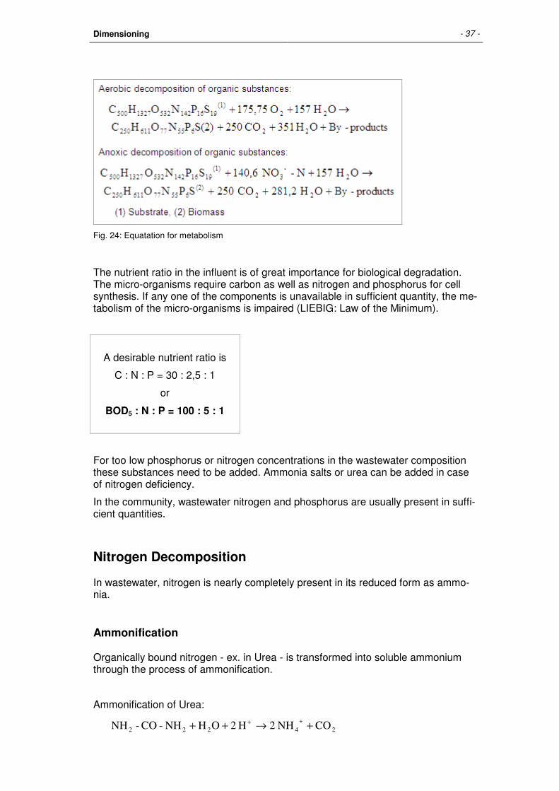
Dimensioning - 37 -
Fig. 24: Equatation for metabolism
The nutrient ratio in the influent is of great importance for biological degradation. The micro-organisms require carbon as well as nitrogen and phosphorus for cell synthesis. If any one of the components is unavailable in sufficient quantity, the me-tabolism of the micro-organisms is impaired (LIEBIG: Law of the Minimum).
A desirable nutrient ratio is
C : N : P = 30 : 2,5 : 1
or
BOD5 : N : P = 100 : 5 : 1
For too low phosphorus or nitrogen concentrations in the wastewater composition these substances need to be added. Ammonia salts or urea can be added in case of nitrogen deficiency.
In the community, wastewater nitrogen and phosphorus are usually present in suffi-cient quantities.
Nitrogen Decomposition
In wastewater, nitrogen is nearly completely present in its reduced form as ammo-nia.
Ammonification
Organically bound nitrogen - ex. in Urea - is transformed into soluble ammonium through the process of ammonification.
Ammonification of Urea:
24222 CO NH 2H 2 OH NH-CO-NH +→++++

- 38 - AQUA DESIGNER
If it goes directly into the receiving water, ammonium oxidises to nitrate in the self-purification process. The oxygen requirements are high for nitrification and, as a result, the oxygen concentration in the surface waters would be considerably re-duced. This leads to further oxygen depletion of eutrophic waters. Furthermore, in surface waters, ammonium when twelve times lower in concentration than nitrate has a disturbing influence on biological processes. Therefore, it is useful to go through the nitrification process in the wastewater plant itself.
For every one ammonium molecule that is formed one H+-Ion is used. Initially, this has a positive effect on the buffer capacity of the wastewater. The equation for nitri-fication will show that H+-Ions are released and the buffer capacity of the water is again reduced.
Nitrification
The nitrification process has various negative effects on the condition of natural (surface) waters. Therefore, it is desirable to go through the nitrification process within a controlled technical system.
The autotrophic nitrifying bacteria nitrosomonas and nitrobacter gain energy for their metabolism and cell synthesis from oxidising ammonium.
The oxidation of ammonium takes place in two steps:
1. Nitrosomonas: Nitrite
++++→+ H 4 OH 2 NO 2 O 3 NH 2 2
-
224
2. Nitrobacter: Nitrate
-
32
-
2 NO 2 O NO 2 →+
The carbon source for the nitrifying bacteria is inorganic carbon, ex. the dissolved CO2. Dissolved CO2 is available from the metabolism of heterotrophic microorgan-isms and the degradation of organic compounds.
Denitrification
The nitrogen has been transformed from the reduced form to the oxidised form by nitrification. However, it is still present as nutrient in the wastewater. By denitrifica-tion the soluble nitrate and nitrite nitrogen are transformed to elementary nitrogen or, in the worst case, to a slight degree reduced to N2O (laughing gas, nitrous oxide) and escape as gas.
A large part of the heterotrophic micro-organism is able to satisfy its oxygen de-mand by reduction of nitrate and nitrite nitrogen when dissolved oxygen is not pre-sent. The portion of these organisms in relation to the total existing heterotrophic micro-organisms present in the system generally is between 70 and 90 %.
The basic equation for the denitrification is as follows:
2223 O 2,5 OH N H 2 NO 2 ++→+ +−

Dimensioning - 39 -
Denitrification is achieved, for example, by aerating and mixing the wastewater al-ternately and mixing it only after meeting an upper limit for nitrate concentration. The heterotrophic bacteria use the nitrate as energy source during the non aerated phases. The aeration switches on again after a lower limit for the nitrate concentra-tion is reached. This technique is called intermittent denitrification.
Almost complete denitrification is achieved by using a time switch in case of un-available measuring techniques for automating the denitrification process.
Phosphorus Decomposition
Phosphorus in the wastewater is predominantly present as orthophosphate. The soluble inorganic polyphosphates and organic phosphorus compounds are trans-formed into orthophosphates in the course of the decomposition processes. This is the only form for cell uptake by the micro-organisms.
Biological Phosphorus Removal
The natural P-content of the dry cell mass is around 3%. Phosphorus has an impor-tant role, for example, in the energy metabolism with the energy carriers ADP/ATP.
Phosphorus is stored as polyphosphate in different cell compartments in the en-hanced biological uptake of phosphorus.
An enhancement of phosphorus in the activated sludge is promoted by the alterna-tion of aerobic and anaerobic conditions where P-storing bacteria are particularly well adapted. For this, an anaerobic tank can precede the activated sludge tank. This technique is not included in the current version of the program.
The anaerobic phase can be integrated in the processes of the activated sludge tank especially with the methods of simultaneous aerobic sludge stabilisation and intermittent aeration by prolonging the unaerated phase over the Deni-phase. True anaerobic conditions then exist in the activated sludge tank./10/
Anaerobic Volume
The anaerobic phase should not be included into the evaluation of the sludge age as there is very reduced biological activity and barely any sludge growth present. Thus an anaerobic volume should be added to the activated sludge volume.
The calculation of the anaerobic volume is based on a publication by the Technical University Darmstadt /17/.
The following qualifying factors encourage biological phosphorus removal.
• decomposed raw sewage, for example, generated from pressure pipes with organic acid concentrations of >= 50 mg acetic acid/l
• BOD1/BOD5 ratio >= 0.3 or BOD5-filtrate/BOD5-original >= ca. 0.4
• Industrial wastewater with high organic load
• N/BOD5 ratio in the denitrification inflow <=0.25
• None or short presedimentation
• mechanical thickening of primary and excess sludge

- 40 - AQUA DESIGNER
• low P-load following the sludge treatment
• Separate sewerage system with little extraneous water
The computation is based on the contact time during the anaerobic phase. The dry weather inflow and the return sludge must be taken into account when dimensioning the anaerobic tank.
Boll/17/ recommends an anaerobic contact time of 0.75 – 1.0 hours for the ideal case when most of the above listed conditions apply.
For less ideal conditions, he recommends a contact time of 1.0 – 2.0 hours. This recommendation is also valid for activated sludge systems with simultaneous sludge stabilisation and low loading.
AQUA DESIGNER suggests an anaerobic contact time of 1.0 h on the basis of the recommendations for the biological phosphorus removal with intermittent aeration and the recommendations of Boll.
Chemical Phosphorus Removal
A limit of 2,0 mg/l for phosphorus concentration during the operational process is not always maintained with biological phosphorus removal. Therefore, it is neces-sary to provide for a chemical precipitation step. The chemical precipitation is a phase transition process where dissolved phosphate forms an insoluble compound with another dissolved precipitant/flocculant and sediments in the secondary sedi-mentation tank.
For this process the precipitants FeCl3 and AlCl3 are available in the program.
Dimensioning - 41 -
Handling
Title- and Menubar
Path name and file name of the current file are on the Titlebar.
On the Menubar, only the file menu is active until completion of the computation. However, the language menu is an exception: You can switch at any time between English and German.
In the Main Window frame the project name is displayed. For the case File > New, no name initially appears as the project name.
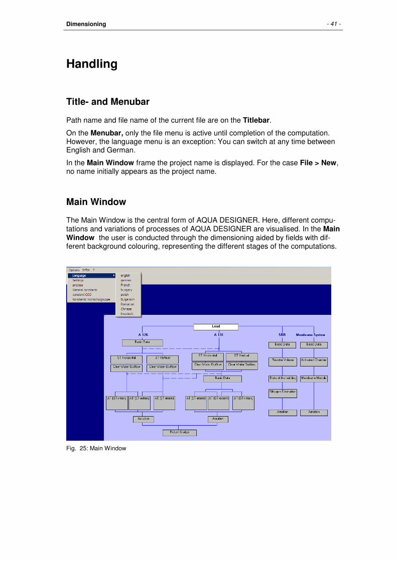
Main Window
The Main Window is the central form of AQUA DESIGNER. Here, different compu-tations and variations of processes of AQUA DESIGNER are visualised. In the Main Window the user is conducted through the dimensioning aided by fields with dif-ferent background colouring, representing the different stages of the computations.
Fig. 25: Main Window

- 42 - AQUA DESIGNER
Advantages of the Main Window
• Access to completed computations and dimensioning results is possible at any time
• Corrections can begin on any level of the tree diagram
• Variations can be calculated in parallel and can also be compared
• Variations of methods presented as flow diagrams in the Main Window
• Conduction through the AQUA DESIGNER steps with coloured fields
• Display of the most current computation status and options
Fields
Main window fields, in principal, are links where the different forms for input and computation are found.
Different background colouring represent the different stages of the design work and computation. So the different choices in the most current computation are marked by white backgrounds. For example, opening the Main Window with File > New only the field Load has a white background.
The field is marked green after completion of the respective computation. Unavail-able fields are marked grey.
The dimensioning of the biological treatment step is completed when one passage of the diagram beginning from Load and ending at Return Sludge has been com-pletely calculated and is, thus, marked green all the way through.
Fig. 26: Completed Computation
Dimensioning - 43 -
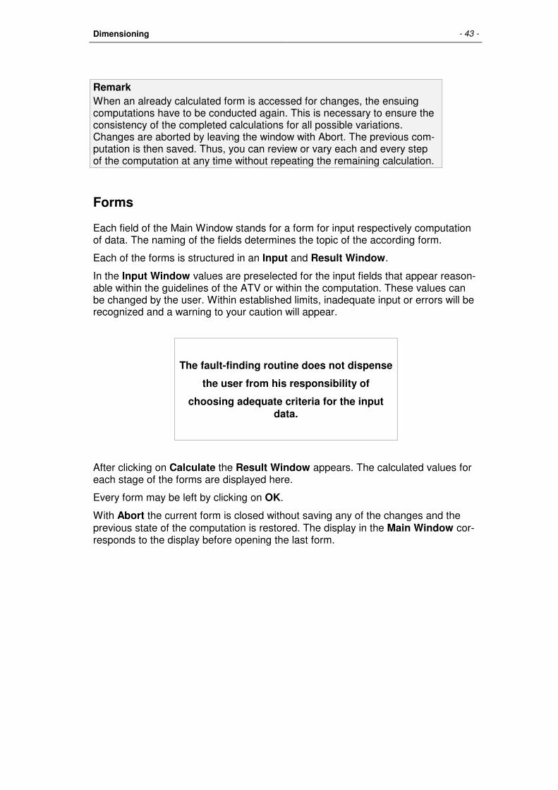
Remark When an already calculated form is accessed for changes, the ensuing computations have to be conducted again. This is necessary to ensure the consistency of the completed calculations for all possible variations. Changes are aborted by leaving the window with Abort. The previous com-putation is then saved. Thus, you can review or vary each and every step of the computation at any time without repeating the remaining calculation.
Forms
Each field of the Main Window stands for a form for input respectively computation of data. The naming of the fields determines the topic of the according form.
Each of the forms is structured in an Input and Result Window.
In the Input Window values are preselected for the input fields that appear reason-able within the guidelines of the ATV or within the computation. These values can be changed by the user. Within established limits, inadequate input or errors will be recognized and a warning to your caution will appear.
The fault-finding routine does not dispense
the user from his responsibility of
choosing adequate criteria for the input data.
After clicking on Calculate the Result Window appears. The calculated values for each stage of the forms are displayed here.
Every form may be left by clicking on OK.
With Abort the current form is closed without saving any of the changes and the previous state of the computation is restored. The display in the Main Window cor-responds to the display before opening the last form.

- 44 - AQUA DESIGNER
Loading
The values for calculating the inflow sewage loads and water volumes are entered in the form Load. Apart from data of the municipal loading, industrial wastewater loads and internal response as turbid water may be incorporated.
Fig. 27: Form on loading selecting all parameters
ATV-DVWK-A 198 from april 2003 is basis for calculating loading parameters.
The evaluated Loads can be edited.
Industrial parts has to be entered by the user.
If you select the primary sedimentation, you get the reduced loads and concentra-tions depending on the retention time. This values are valid for the biology.

Dimensioning - 45 -
Input Options
The form Load enables you to enter inflow data individually and flexibly. It is possi-ble to enter the hydraulic data and constituents as specific or absolute values. They may also be entered as inflow concentrations. From the selected type of values the corresponding values are automatically calculated.
Fig. 28: Form on loading, selecting the option for specific values
Specific Values
The option on specific values is active upon opening a new project and the form Loads. First enter the Population Equivalent before selecting a different option for the load values. This step is required for the automated conversion of values within the different options.
After entering the PE you may change to the option for absolute values. If you do this, please read the part on absolute values of the handbook.
ATV standard values are preselected for municipal wastewater sewage loads and volumes. These values may be changed independently.
Industrial and trade loading are entered by the AQUA DESIGNER user.
Municipal Loading
The population equivalent in the window population equivalent only encounters the municipal wastewater load.
The input is limited to values ranging between 50 and 3 000 000 inhabitants.
Wastewater Inflow
After entering the Population Equivalent, a peak factor will be presetted, based on the ATV-DVWK A 198 /56/.
The evaluation of specific values and water amounts is mainly based of chapter 4.2.3, „Abflussdaten anhand von Erfahrungswerten“.

- 46 - AQUA DESIGNER
Dry weather flow
QT,aM = QS,aM + QF,aM l/s
slqGGAEdwSEZ
aMQS /*,86400
,*, +=
Daily peak flow at dry weather for the yearly average
aMQFxQ
aMQSQT ,
max
,*24max, +=
For the divisor xQmax an intervall is given, which defines the interval between QT,h,max and QT,2h,max. AQUA DESIGNER presets the lower value QT,h,max.
Fig. 29: Divisor xQmax depending on PE /56/
The rain water flow QM will be evaluated by fS,QM. Also this value will be interpo-lated, depending on the PE.
Fig. 30: Interval of fS,QM for the evaluation of the rainwater flow to the wwtp /56/

Dimensioning - 47 -
QM = fS,QM * QS,aM + QF,aM
Deutsch:
QT,aM Yearly average of dry weather flow l/s
QS,aM yearly rainwater flow l/s
QF,aM Yearly average of infiltration water l/s
wS,d specific wastewater amount 100 – 150 l/(E*d)
fS,QM Factor for the evaluation of the acurate rainwater inflow
l/s
The infiltration water has to be estimated by experience and will be entered as a percentage of the domestic wastewater.
Loads
The given loads for organic loading (BOD5), nitrogen (TKN) and phosphate (P) are in accordance with ATV guidelines without consideration of a preliminary step.
In this form, only those values are selected that are relevant for the computation in accordance with both guidelines. The filterable solids are considered in the dimen-sioning based on A131, and are entered later after selecting the computation method.
The daily loads are evaluated using specific loads and the population equivalent.
Daily load = population * specific. load [kg/d]
The specific BOD5-load of 60 gO2/(PE*d) is suggested. This value can be either accepted or modified by the user.
The value of 60 gO2/(PE*d) results from a BOD5-inflow load without a primary sedi-mentation step. When a primary sedimentation step is selected, the value for the specific inflow load decreases depending on the detention period in the primary sedimentation step. The corresponding parameters are available in the ATV A131 guideline.
The same applies to nitrogen and phosphate loads.
Parameter Raw wastewater
Retention time in the presedimentation at Qt
0,5-1,0 h 1,5-2,0 h BSB5 60 45 40 CSB 120 90 80 Abf. Stoffe 70 35 25 N 11 10 10 P 1,8 1,6 1,6 Table 1 from ATV A131 guideline: Wastewater loads in gO2/(PE*d), undershot in 85% of the days, without consideration of sludge liquor

- 48 - AQUA DESIGNER
Absolute Values
It is very useful to enter actual hydraulic masses and waste concentrations or loads from data analysis when they are available.
Select the option for Absolute Values after entering a value for the population equivalent. The window for entering the absolute values appears. Here, values are preselected based on the specific data of the previously entered PE.
AQUA DESIGNER calculates these absolute values based on the ATV guideline recommended specific values and the previously entered population equivalent. This applies to the volumes as well as to the sewage contents.
Fig. 31: Form on loads selecting the option specific values
Wastewater Inflow
In addition to the daily dry-weather flow, a value for extraneous water may be en-tered to enable the conversion from specific values to absolute values. In the spe-cific values option the extraneous water is included in the displayed value for dry-weather flow. The daily extraneous water is not included in the value for daily dry-weather flow.
Loads
In the window for absolute values it is again possible to enter the constituents in two separate ways. For data from analysis that are usually given as concentrations choose the option Concentrations in the window for Absolute Values. AQUA DESIGNER will calculate the load based on the concentrations and the inflow vol-ume.

Dimensioning - 49 -
Fig. 32: Form on load, constituents when selecting concentrations.
In any case, values for the concentrations of constituents will be suggested based on the previously entered and calculated loads.
Now enter the actual concentrations. AQUA DESIGNER calculates the loads based on the concentrations and the inflow when choosing the option loads. The results from the conversion of absolute values to specific values are displayed when choos-ing the option specific values.
Values for extraneous water, dry-weather flow and the daily inflow for different con-stituents have been entered in the window for absolute values. Thus, the fraction of domestic wastewater is known and all specific values can be calculated.
Internal Response
Analysis Supernatant Parameter Minimum
mg/l Maximum
mg/l Average
mg/l BOD5 12 3420 690 COD 70 285002) 2196 Ntot 258 1810 1025 NH4-N 66 1462 746 Ptot 0,4 1169 86 Extract of Table 3 from ATV Arbeitsbericht „Maschinelle Schlammentwässerung /42/“: Concentration in Supernatant and municipal waste water

- 50 - AQUA DESIGNER
COD mg/l
NH4-N mg/l
PO4-P mg/l
Average 8000 550 12 Scale 2000 – 12000 300 – 750 1 – 31 Table 6 from /41/: Concentrations in supernatant of primary sludge thickening (0,45 µ m fitrated)
Handling
Internal responses out of the supernatant of the sludge treatment can be consid-ered very detailled.
Fig. 33: Flow scheme for supernatant flows
Simple Calculation
Concentrations
Concentrations of the supernatant can be entered. The loads of the internal re-sponse will be calculated based on the concentrations and the resulting supernatant amount.
Waste Sludge (WS):
=
d
m
m
kgMLSS
d
kgB
kgBOD
kgSSWS
Q
WS
BODdd
WS
³
³
* 5,
5
0,

Dimensioning - 51 -
Thickened and dewatered waste sludge:
=
d
m
m
kgMLSS
d
kgB
kgBOD
kgSSWS
Q
WS
BODdd
WS
³
³
*
1
5,
5
1,
Supernatant as difference of above volumes:
Load with volume flow and concentrations:
=
d
kg
kg
gl
mgc
d
mQ
BSISI
SId
1000
*³
,
Percentual Part of the Inlet
The internal response can be chosen as a relation of the inlet loads. The relation will be build to the loads before pre sedimentation.
Enhanced Calculation
Especially in larger plants you usually have to steps of thickening respectively de-watering. The concentrations of the supernatant out of the thickening in a first step are very different to the concentrations in the supernatant of the dewatering. Ther-fore an detailled form for the concentrations of these to steps is provided.
Dimensioning
The loads of the internal response will not be reduced by the pre sedimentation. They are directly added to the inflow loads of the biological stage.

- 52 - AQUA DESIGNER
Industrial Loads
A daily water volume of 0 m³/d is preselected for the trade and industrial compo-nent, meaning no commercial or industrial wastewater is present.
Wastewater Inflow
If a trade or industrial component needs to be considered, the daily water volume must be entered in the input Industrial Waste Water.
By leaving the input field, another window opens for entering the wastewater con-centration and the hour index
The hourly wastewater volume results from the daily wastewater volume and hour index.
=
h
m
h
average
di
i
³,
=
h
m
x
dg
g
³,
Qi, Qid hourly or daily industrial inflow, respec-
tively [m³/h]
Qg, Qg,d hourly or daily trade wastewater inflow, respectively
[m³/h]
haverage hour index [h/d] x hourly average [h/d]
Loads
The daily loads for business and industry are evaluated using the given water vol-umes and concentrations.
=
d
kgcQLoadDaily
gigi
1000
* ,,
ci/g concentration of wastewater component mg/l Qi/g wastewater volume current m³/d
Total Load
After entering all basic data, click on the button Calculate. A Result Window with the hourly water volume and daily load appears.
The result contains the municipal, trade, and industrial loads and water volumes.
Leave the form with OK.

Dimensioning - 53 -
Pre Sedimentation
If the Pre Sedimentation has been chosen in the Load-Form, this step also will oc-cure in the main-form.
The volume will be chosen by the retention time of the load form. It is based on the dry weather flow.
If you want to include more than one chamber, you can enter this in under Options.
Choosing an ATV-Guideline
AQUA DESIGNER is designed for wastewater plants with simultaneous aerobic sludge stabilisation. The method is restricted to the activated sludge process with nitrification and intermittent denitrification. Biological and chemical phosphorus re-moval can be included in the computation by selecting the respective parameters.
The basis for the layout of the biology are the ATV guidelines A126 and A131. De-pending on the population equivalent, different characteristic values and directions for the calculations arise for dimensioning.
Fig. 34: Main Window for 500 <= PE <= 5000
For population equivalents over 5000 only the field Basic Data for A131 is active in the Main Window. For population equivalents smaller than 5000 both Basic Data fields are active.

- 54 - AQUA DESIGNER
ATV-A131
The A131 includes the dimensioning of wastewater treatment plants with simultane-ous aerobic sludge stabilisation, and treatment plants with pre-treatment and an-aerobic sludge digestion.
The ATV A131 guideline applies to loads representing a population equivalent of more than 5000. The dimensioning and the evaluation of oxygen demand based on the A131 guideline may also be useful when special clarifying processes for lower population equivalents are required.
The dimension of the secondary sedimentation tanks can be calculated based on the ATV 131 guideline for lower population equivalents as well. This may result in improved tank dimensions under certain influent conditions.
ATV-A126
The ATV A126 guideline is employed for wastewater plants operating with the acti-vated sludge process with simultaneous sludge stabilisation for population equiva-lents of 500 to 5000.
The wastewater plant design based on the ATV 126 guideline is a useful choice in the event of unusually high wastewater volumes with a population equivalent of less than 500.
University Algorythm
You can choose the University algorythm, if the waste water compostion is very different to municipal waste water or to compare the calculation with ATV A 131.

Dimensioning - 55 -
Clarification Method
In AQUA DESIGNER different clarification methods are at your choice. Select the clarification method on the menu bar with Options > Process.
You must restart with the Basic Data form when the method for nitrogen removal is to be changed after a computation has been completed already.
Selecting the method for nitrogen removal is only possible on the level of the Main Window. The menu bar options are inactive while working in computation forms.
The outflow requirements must always be reviewed after selecting a new clarifica-tion method as the previously selected outflow values might not meet with the new conditions. For example the nitrate outflow value must be reviewed in the Basic Data form when the method for nitrogen removal has changed from ‘Only nitrification’ to ‘Intermittent nitrification’.
Fig. 35: Selecting a method for nitrogen removal from the menu bar
Only Carbon Degradation
Dimensioning the biological step solely on the carbon compound degradation is available in the ATV guideline A131.
The sludge age for the sole carbon compound degradation is listed in Table 2 of the A131 guideline.

- 56 - AQUA DESIGNER
Standard of purification up to 20000 PT
more than 100000 PT
Wastewater clarification without nitrification
5
4
Table 2 from the A131:Minimum sludge age in days depending on the standard of purification and the wastewater plant size (Intermediate values are to be estimated)
Values between the population equivalent of 20000 and 100000 are interpolated linear.
In the aeration the factors fC and fN are adapted to the selected method of purifica-tion.
Only Nitrification
Dimensioning the biological step with sole nitrification is available based on the ATV guideline and based on the university algorithm.
ATV-A131 Guideline
The ATV A131 guideline also gives reference values for the required sludge age in nitrification.
Standard of purification
<= 20000 EW > 100000 EW
10°C 12°C 10°C 12°C Wastewater clarifi-cation with nitrifica-tion
10 8,2 8 6,6
Table 2 from ATV-A131
Oszilation factor <= 20000 EW > 100000 EW SF 1,8 1,45
Intermediate values has to be interpolated.
Aerobic sludge adge:
TSS,A = SF * 3,4 * 1,103(15-T) [d]
SF = safety factor for nitrification
If there are longer periods with a temperature less than 12°C, the dimensioning has to be done with 10°C.

Dimensioning - 57 -
ATV-A126 Guideline
Selecting the ATV-A126 automatically includes the aerobic sludge stabilization method. Here the dimensioning based on the sole nitrification method must be re-viewed for economical reasons.
University Algorithm
The dimensioning based on the university algorithm is described separately.
Nitrification and Denitrification
Generell
Three methods, the combined nitrification/denitrification, the simultaneous and the intermittent denitrification, are available for dimensioning the biological step on the basis of nitrification and denitrification.
ATV-A126
The dimensioning based on the ATV A126 guideline only applies to the intermittent denitrification. The selected method of clarification only affects the aeration period.
ATV-A131 Basis BSB
First the aerobic sludge age is calculated based on the following equation:
[ ]dSFt TSS
)15(103,1*4,3* −=
Total sludge age:
[ ]d
V
VSFt
AT
D
TSS
−
= −
1
1*103,1*4,3* )15(
Denitrification ratio
Simultaneous, intermittend denitrification:
][*9,2
*75,0
5
,
,5
,3
mgBOD
mgN
V
VOU
C
S
AT
DBODC
ZBBOD
DNO=
Separate stage denitrification:

- 58 - AQUA DESIGNER
][**9,2
**
9,2
*75,0
5,
,2
75,0
,
,5
,3
mgBOD
mgN
CQ
SQ
V
VOU
C
S
ZBBOD
ABORI
AT
DBODC
ZBBOD
DNO−
=
Oxygen demand:
][**17,01
**15,056,0
5
2
,kgBOD
kgO
FTt
FTtOU
TS
TSBODC
++=
Interpolated Values:
Fig. 36: Table 4 from ATV A131, 4/99 for 10°C-12°C
Case: separate stage, alternated denitrification
0,13 capacityation denitrific 0,11 ≤≤
2,011,0*11,013,0
2,03,0
5
,3+
−
−
−=
BOD
S
V
V DNO
AT
D
0,15 capacityation denitrific 0,1 ≤<
3,013,0*13,015,0
3,05,0
5
,3+
−
−
−=
BOD
S
V
V DNO
AT
D
Case: simultaneous, intermittend denitrification
0,15 capacityation denitrific 0,05 ≤≤

Dimensioning - 59 -
2,006,0*06,015,0
2,05,0
5
,3+
−
−
−=
BOD
S
V
V DNO
AT
D
Way of Calculation:
tss = f(VD/VAT, T):
[ ]d
V
VSFt
AT
D
Tss
−
= −
1
1*103,1*4,3* )15(
OUC = f(T,tSS) :
++=
5
2,
**17,01
**15,056,0
kgBOD
kgO
FTt
FTtOU
SS
SSBODC
ATV-A131 Basis CSB
=
mgCOD
mgN
C
S
C
S
ZBBOD
DNO
ZBCOD
DNO
,
,3
,
,3*5,0
=
mgCOD
mgN
V
VOU
CODC
S
AT
DBODC
ZB
DNO*
9,2
*75,0*5,0 ,
,
,3
Oxygen uptake:
−−=
d
kgOXSCQOU WSSTeinertATid
Cd2,,,
,1000
)(*
−−=
kgCOD
kgO
B
XSCQdOU
CODd
WSSTeinertATi
C2
,
,,,
1000*
)(*
OUc oxygen uptake for carbon removal kg/kg OUd,c daily oxygen uptake for carbon removal kg/d Sinert, e,ST concentration effluent sedimentation tank mg/l XWS concentration of waste sludge mg/l Ci, AT concentration influent activated tank mg/l
The subsequent calculations are found in the Basic Data chapter beginning from the section on sludge age.

- 60 - AQUA DESIGNER
Variant dimensioning temperatures
A 131, 2000 recommends to increase the denitrification capacity at the dimension-ing temperatures higher than 10 – 12°C by 1 % per 1°C. According to both edditions of A 131 this is applied to the denitrificaton at the upstream process stage. The for-mulas for intermittent and simultaneous denitrification are available. Here the in-creased dimensioning temperature has its influence.
The denitrification proportion for the following required denitrification capacity is determined for the increased dimensioning temperature
According to A 131,2000:
01,0*)12(1
1*
5
3
5
3
−+
−=
−
TBSB
NNO
BSB
NNO D
T
D
University Algorithm
The dimensioning based on the university algorithm is described in a seperate chapter.
Intermittent Denitrification
The oxidation of ammonium to nitrate and the reduction of nitrate to water is managed by alternate aerated and unaerated periods in the intermittent deni-trification. The unaerated period per day is equal to the evaluated ratio of the denitrification volume to the total volume. This evaluated aeration period is suggested in the programs aeration window.
This implies that the aeration period in intermittent denitrification must be designed larger than the aeration periodin the combined nitrification/denitrification and the simultaneous denitrification.
The mixing devices are designed for the total volume.
The good controllability and the theoretically high denitrification rates by high inter-nal recirculation are the advantages of the intermittent denitrification method. While in the combined nitrification/denitrification method a maximum recirculation rate of 4 is recommended the completely mixed tanks may be suggested for recirculation rates of 20.

Dimensioning - 61 -
Seperate Stage Denitrification
The required recirculation rate results from the outflow requirements for ammonium and nitrate.
Recirculation rate (RZ):
1][][
][][
33
4 −−−−
−−=
oNNOeNNO
eNNHoNRZ total
From this value the return ratio must be deducted to get the internal recirculation rate.
Internal recirculation:
RC = RCtotal – RS
RS = Return sludge ratio
The graphical surfaces and the constructional values are not available to the same extend in the combined nitrification/denitrification method as is the case for the other clarification methods. A separation into denitrification and nitrification volume for the constructions are not yet available in this AQUA DESIGNER version.
External tanks are available as circular tanks or rectangular tanks after deciding on the secondary sedimentation tank. In the form A131 for the activated sludge tank the external measurements of the construction are determined. A separation into nitrification and denitrification tank is not available in the graphical display. In the computation and the documentation ,however, the separation is included and con-firmed.
The values given in the A131 form on the activated sludge tank, however, are suffi-cient to determine the aeration and mixing.
An aeration period of 24 hours and aeration without separate mixing in the nitrifica-tion tank are suggested in the A131 aeration form when combined nitrifica-tion/denitrification is selected.
The mixing design is based on the denitrification volume only.
The type and size of the screens are determined in the graphical surface on mem-brane aeration.
The drawing of the tank shows the nitrification volume only.
Drawings covering the whole biology are not available in the combined nitrifica-tion/denitrification. A print out of the nitrification tank is available. Thus, a graphical display of the distribution of the aeration is possible for documentation.
The calculation of operation costs is fully available in the combined nitrifica-tion/denitrification. The recirculation rate is included into the calculation of operation costs.

- 62 - AQUA DESIGNER
Cascaded Denitrification
Generell
Cascaded Denitrification means that waste water or sludge will run through subse-quent basins, i.e. a basin cascade. The procedural advantages of a Cascaded Deni-trification arise from the way the waste water stream is distributed to the cascades.
In the simplest form the returned activated sludge is fed to the first cascade, while the incoming material is equally distributed to all of the cascades.
Fig. 37: MLSS for RS = 1 resp. QRS = Qges; “TS” means SS
The figure above shows a cascade of four stages. 25% of the inlet is distributed to each of the cascades. The recirculation ratio for the following explanations is as-sumed to be RV = 1. The Cascaded Denitrification offers two procedural advan-tages that allow for higher constructural expenditures under certain circumstances.
MLSS-Concentration
Since the waste water inlet is equally distributed to the cascades the mixing ratio of inlet and return sludge corresponding to the ratio of an uncascaded basin is only reached within the last cascade.
MLSS in the first basin:
==
+=
³40,6*
25,1
1
25,0*
*1,
m
kgSS
SSQSS RS
totRS
RSRSAT
with SSRS = 8 kg/m³ and QRS = Qges

Dimensioning - 63 -
MLSS in the second basin:
==
+
+=
³33,54,6*
5,1
25,1
5,0*
*)25,0*( 1,
2,m
kg
SSQQSS
totRS
ATtotRS
AT
MLSS in the third basin:
==
+
+=
³56,433,5*
75,1
5,1
75,0*
*)5,0*( 2,
3,m
kg
SSQQSS
totRS
ATtotRS
AT
MLSS in the fourth basin:
==
+
+=
³99,356,4*
2
75,1*)75,0*( 3,
4,m
kg
SSQQSS
totRS
ATtotRS
AT
Average MLSS with equal distribution to equally sized basins:
=
+++=
³1,5
4
99,356,433,540,6
m
kgSS AT
The average MLSS increases because of keeping the basins as cascades from 4,00 to 5,10 kg/m³.
SSAT MLSS in the Chamber kg/m³ SSRS MLSS in the Return Sludge kg/m³ QRS Return sludge volume m³/h Qtot Total inflow m³/h SSi Inflow MLSS for each chamber kg/m³
Separate Stage Denitrification
The Cascaded Denitrification is mostly connected to a separate stage denitrification. Should the separate stage denitrification be represented by several cascades which succeed each other, it will be possible to denitrify the nitrate from denitrification stage n in the following denitrification stage n+1.
Assuming a complete nitrification and denitrification (as for the separate stage deni-trification) within the basins an efficiency factor depending on the number of stages can be determined.
( ) ( )eNNORSQNNHn
QNit −+=− 34 *)1(**
( )( ) ( ) )1(*
11
33
3
RSnNNONNO
NNO
eD
DD
+−=
−+−
−=η

- 64 - AQUA DESIGNER
Since the denitrification‘s efficiency factor arises from a pure mass balance where a complete nitrification and denitrification in the individual stages is assumed the ni-trate outlet is not mentioned; it is a part of the mass balance.
Intermitting, Simultanuous Denitrification
Within the intermitting denitrification the possible nitrate reduction is not restricted by the mass flow in defined zones. The theoretical recirculation rate compared to the separate stage denitrification is relatively high. Therefore the possible nitrate reduction is governed by the denitrification capacity.
Given outlet values for ammonia and nitrate are resulting in necessary denitrification capacity and denitrification ratio. Looking at the balance of the cascade basins it is obvious that the mass balance for each basin is the same.
This condition is valid assuming a BOD5-concentration of 0 mg/l in the return sludge. Even if assuming a BOD5 value of more than 0 only a slight change in the necessary denitrification capacity and the resulting denitrification ratio will be ob-served.
Following those assumptions the denitrification ratio in each cascade basin is the same, should you have chosen intermitting denitrification. The same is true for the simultanuous denitrification.
Operating
Choosing Process
Regardless of which denitrification procedure you have chosen (i.e. intermitting, simultanuous or separate stage denitrification) you are able to choose cascaded denitrification. Your chosen denitrification process will then be assumed to take place within the individual cascade basin.
Therefore Cascaded Denitrification means a combination of a denitrification proce-dure and a certain arrangement of the basins within the cascade.
In the menu bar choose Options > Process. Within the nitrogen elimination a cleaning process is always given as an option. You can now tick the Cascaded De-nitrification on or off.
User Screen
Should you have chosen Cascaded Denitrification then there will only be a little more input for the Form Basic Data necessary.
Giving the separate stage denitrification the nitrate outlet concentration is given by the mass balance. Given the simultanuous and the intermitting denitrification the denitrification ratio results from the nitrate outlet value.

Dimensioning - 65 -
The dry solid concentration is caclulated by the dry solid concentration within the return sludge and the mixing ratio.
As soon as you have finished the input in the form basic data you reach the screen Calculation Data for the Cascaded Denitrification by hitting OK. Here you have ex-tensive tools at your disposal that allow for a multitude of different dimensioning variations for the Cascaded Denitrification.
Fig. 38: Form Cascaded Denitrification
Number of Cascades
From the list Number of Cascades you can choose up to four cascades.
Volume of Cascades
The necessary volume of the cascades is calculated on the basis of the current in-put data and is equally distributed on each cascade. You can edit the proposed val-ues of the volumina in the text fields Volume, i.e. you can define different volumina to each cascade. If you choose smaller or larger volumina as they are defined by the minimum dimensioning process new dimensions, based on your choice, will be calculated. Therefore the sludge can in- or decrease compared to the minimum di-mensioning process.
You can define own values for the cascade volume and the distribution by entering those into the text fields. If you choose the option As Input Data all the calculations will be based on your defined values. As it is the case in the calculation without cas-cades the results in the proof calculation differ from the minimum dimensioning.

- 66 - AQUA DESIGNER
Variations
The cascades can be loaded and designed using different ways. AQUA DESIGNER allows for the following cases:
• Calculation on basis of directly entered volumina and ways of loading
• Calculation for same volumina. You can choose the loading, thus the volu-mina remains the same.
• Same loading and same volumina. For the operation it is best to have the same operational conditions in each basin. That makes it more manageable and controllable for the operating personal.
• Same volumina and same sludge loading. The sludge loading is crucial to the biological processes. The same sludge loading is reached by chosing dif-ferent loading rates for the cascade basins. If you have chosen this option the loading rate is calculated through an iteration process.
• Same volumina, loading rate and denitrification conditions. This setting is the most manageable concerning operation. Each basin will be dealt with equally and each basin has the same geometry. You will certainly have different sludge loading rates. Using a state of the art measurement and regulating equipment the aeration is adjusted independently. It is not mathematically possible to have the same denitrification conditions in ieach basin. There will always be different conditions for BOD5/NO3 as in the following basins, since at this point only nitrate from the returning sludge is denitrified.This is solved by increasing the denitrification volume in the first basin. The overall volume of the basin is not changed, therefore the nitrification volume de-creases.Since the aerobic volume is reduced the system is calculated re-peatedly until the aerobic sludge age is within an acceptable range. I.e. same denitrification conditions lead to a overall volume that is slightly higher than that which is necessary for a minimum dimensioning.
Results
The calculation screen shows the results in detail. The design parameters of each cascade are shown. Additionally the mass balance of each cascade basin is given according to the freight in a tabular format.
The overall results result form the average contents of dry solids in the whole sys-tem and the nitrogen balance.
Simultaneous Denitrification
The aeration period is suggested as 24 hours as is the case in the combined nitrifi-cation/denitrification. The mixing devices are designed for the total volume.
The regulation of the simultaneous denitrification is inexact as nitrification and deni-trification periods are induced by the change of aerated and unaerated periods.
In the calculation based on the university algorithm the respiration elevation factor for simultaneous denitrification is set as a = 1. This is explained separately in the chapter on the university algorithm.

Dimensioning - 67 -
Simultaneous Aerobic Sludge Stabilization
Sludge stabilization is available in the Basic Data form. Click on the control box for Sludge Stabilization in the algorythm-frame. A sludge age may be preselected when sludge stabilization is chosen.
The sludge load, volumetric loading and the resulting required tank volume are computed after entering the sludge age and the TS-(MLSS-) concentration in the inflow and in the activated sludge tank.
A sludge age of 25 days is recommended for simultaneous sludge stabilization to guarantee the sludge stabilization in temperatures of 10 Degrees C as well. Several Operators ,however, consider a sludge age of 20 days as satisfactory. In this case a partially incomplete sludge stabilization in the winter months is accepted.
Standard of purification plant size up to
20.000 PE more than
100.000 PE wastewater clarification with nitrification, denitrifi-cation and sludge stabili-zation
25
not recommended
Table: Sludge age from ATV A131, Table 2
Three different sludge ages are calculated when simultaneous aerobic sludge stabi-lization and a method for denitrification have been selected.
The minimum required aerobic sludge age is the minimum required sludge age at the selected dimensioning temperature for guaranteeing a stable nitrification.
The VN/V ration is calculated for the preselected sludge age. From this the aerobic sludge age for sludge stabilization results.
After deciding on the activated sludge tank the actual sludge age is again calcu-lated. The real aerobic sludge age results with VN/V.
ATV A126
There is no verification of the sludge age in the computation based on the ATV A126 guideline. It is not possible to influence the dimensioning of biological proc-esses by the sludge age. ´
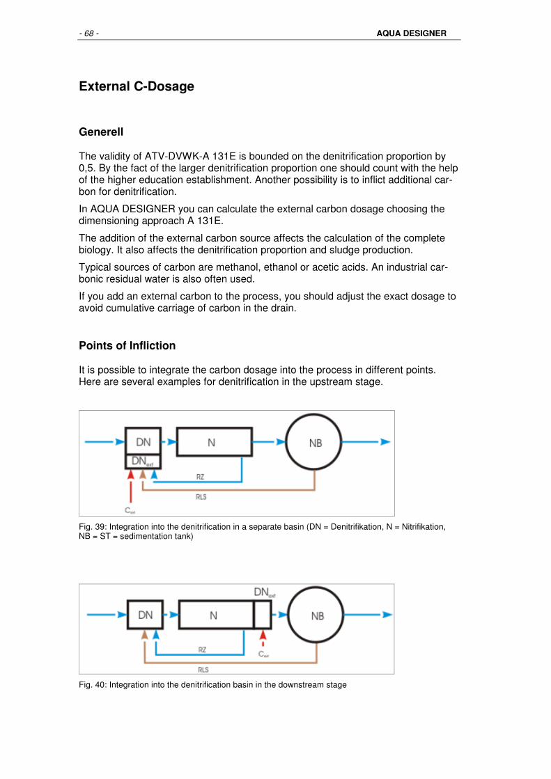
- 68 - AQUA DESIGNER
External C-Dosage
Generell
The validity of ATV-DVWK-A 131E is bounded on the denitrification proportion by 0,5. By the fact of the larger denitrification proportion one should count with the help of the higher education establishment. Another possibility is to inflict additional car-bon for denitrification.
In AQUA DESIGNER you can calculate the external carbon dosage choosing the dimensioning approach A 131E.
The addition of the external carbon source affects the calculation of the complete biology. It also affects the denitrification proportion and sludge production.
Typical sources of carbon are methanol, ethanol or acetic acids. An industrial car-bonic residual water is also often used.
If you add an external carbon to the process, you should adjust the exact dosage to avoid cumulative carriage of carbon in the drain.
Points of Infliction
It is possible to integrate the carbon dosage into the process in different points. Here are several examples for denitrification in the upstream stage.
Fig. 39: Integration into the denitrification in a separate basin (DN = Denitrifikation, N = Nitrifikation, NB = ST = sedimentation tank)
Fig. 40: Integration into the denitrification basin in the downstream stage

Dimensioning - 69 -
Fig. 41: Only the denitrification of the return sludge with external C
Milieu Conditions
The denitrification is affected by several different parameters. Besides the kind of the substate, resp. its disposability for the microorganisms, you should take into account the milieu conditions. The essential parameters are the concentration of the solute oxygen, the temperature and the pH.
Oxygen Concentration
An increasing oxygen concentration slows down the denitrification. In the literature you can find contradicting information concerning the dimension of the obstraction. Generally one can assume that the oxygen concentration of 0,2-0,5 mg/l is toler-able. As the oxygen solubility is stongly affected by the temperature, it was sug-gested that one should rate the obstraction according to the relative saturation /55/. According to Metcalf & Eddy /56/ simplified linear connections between oxygen con-centration and denitrification are specified. So with the concentration of 0,5 mg/l the denitrification level is only 50% and with 1 mg/l it goes towards zero. The most of the other authors go by the assumption of a non-linear connection, what also relates better in congruence with the generall kinetics of biological processes. The impact of the concentration of the solute oxygen is represented according to the different information sources by the illustration /17,50,52/ .
Fig. 42: Correction for the solute oxygen

- 70 - AQUA DESIGNER
For calculations in AQUA DESIGNER it is assumed, that the level of the solute oxy-gen concentration is so low, that the denitrification is not affected. If you want to take the impact of the solute oxygen into account, you can change the speed of the denitrification.
Temperature
As a matter of principle the impact of the temperature on the denitrification level is also dependent on the kind of the substate. But according to the previous experi-ments a differentiation makes no sense. The correction factor for the temperature is represented according to the different information sources by the illustration /17, 52, 53, 54, 2/ .
Fig. 43: Correction of temperature
PH-Value
Also the impact of pH is dependent on the substrate. If the sludge is well adopted, the impact is normally less. The optimal level for the denitrification is approximately ph 7-8. The impact is represented according to the different information sources by the illustration /53, 54, 50/.

Dimensioning - 71 -
Fig. 44: Correction of pH
Calculation
If the denitrification proportion resulted from an unfavourable BOD5/N-Proportion is larger than 0,5, you get the clue.
Message: The denitrification proportion is larger than 0,5. Choose the help of the higher education establishment or the external C-dosage to calcu-late this special case.
AQUA DESIGNER performs no calculations acoording to A 131E in this case.
In order to avoid high denitrification proportions, substates with high percentage of carbon can be added. To find out the required quantity and the impact on the calcu-lation, choose the selection box external carbon.
Fig. 45: External C-Dosage

- 72 - AQUA DESIGNER
A window to specify the basics for carbon infliction would appear.
Different dosage means would be provided in a panel. The material characteristics are taken from the AQUA DESIGNER data base and would be here presented.
Calculation basics
The proportion of denitrificated nitrate to carbon determines the denitrification pro-portion. This interrelation for simultaneuos and intermittent denitrification is stated in A 131E.
=
5
5,
,5
,3*
9,2
*75,0
mgBOD
mgN
V
VOU
C
S
AT
DBODC
IATBOD
DNO
The formula for the denitrification in the upstream stage is printed in yellow. In the valid version of the A 131E this interrelation for the denitrification in the upstream stage is only presented in a form of a chart.
=
−
5
765,0
,
,5
,3*
9,2
*75,0
mgBOD
mgN
V
VOU
C
S
AT
DBSBC
IATBOD
DNO
By the factor of 0,75 the decelerated respiration reaction while using nitrate instead of oxygen is taken into account.
During the process of the denitrification 2,86 g of oxygen per one gramm of nitrate-nitrogen are regained and used during the oxidation of organic substances. (2,86 g O2/g NO3- N).
The above-mentioned relations are valid for 12°C. Varien temperaturen are taken into account through the following formula:
01,0*)12(1
1*
5
3
5
3
−+
−=
−
TBOD
NNO
BOD
NNO D
T
D
The denitrifikation is a respiration process. For the decrease of the oxygen demand the following formula is valid
++=
5
2,
**17,01
**15,056,0
kgBOD
kgO
Ft
FtOU
TSS
TSSBODC
FT = 1,072(T-15) Temperature factor
The relation between the proportions BOD5/N und VD/V for different denitrification methods can be stated in curves. These curves you can find in the chapter Denitri-fication in this Handbook. The nitrogen balance for determination of denitrificated nitrate-nitrogen is also described there.
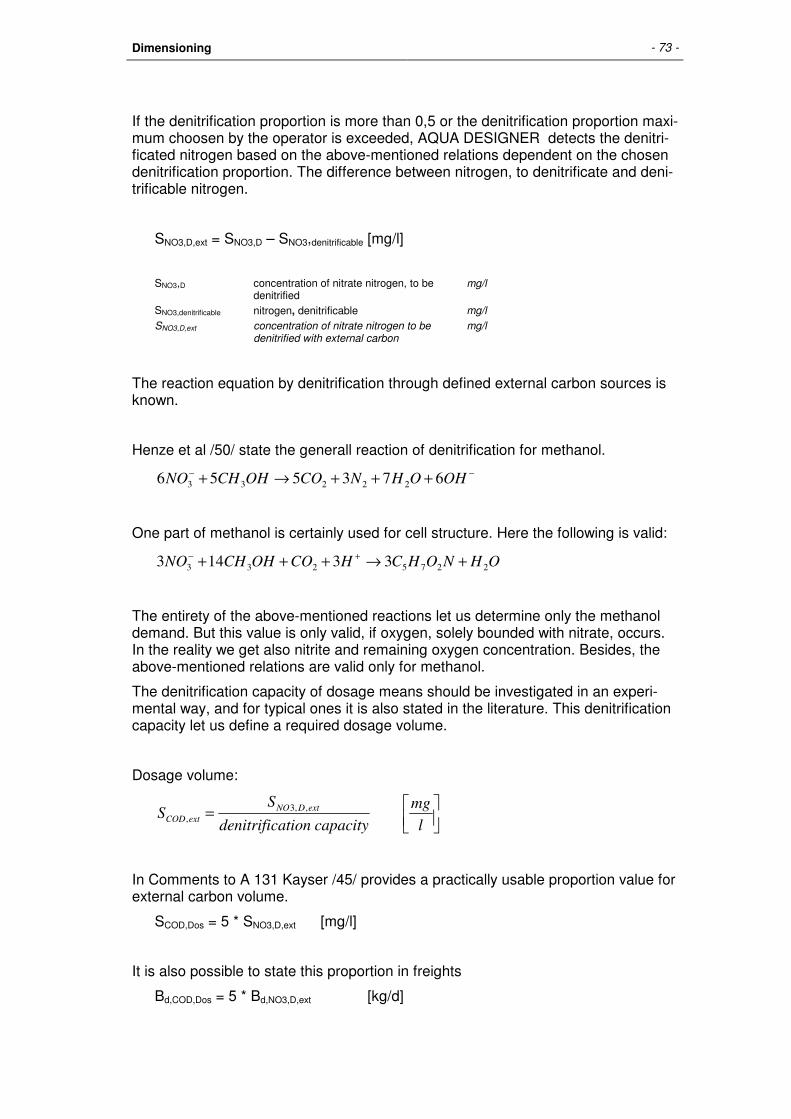
Dimensioning - 73 -
If the denitrification proportion is more than 0,5 or the denitrification proportion maxi-mum choosen by the operator is exceeded, AQUA DESIGNER detects the denitri-ficated nitrogen based on the above-mentioned relations dependent on the chosen denitrification proportion. The difference between nitrogen, to denitrificate and deni-trificable nitrogen.
SNO3,D,ext = SNO3,D – SNO3,denitrificable [mg/l]
SNO3,D concentration of nitrate nitrogen, to be
denitrified
mg/l
SNO3,denitrificable nitrogen, denitrificable mg/l SNO3,D,ext concentration of nitrate nitrogen to be
denitrified with external carbon mg/l
The reaction equation by denitrification through defined external carbon sources is known.
Henze et al /50/ state the generall reaction of denitrification for methanol.
−− +++→+ OHOHNCOOHCHNO 673556 22233
One part of methanol is certainly used for cell structure. Here the following is valid:
OHNOHCHCOOHCHNO 2275233 33143 +→+++ +−
The entirety of the above-mentioned reactions let us determine only the methanol demand. But this value is only valid, if oxygen, solely bounded with nitrate, occurs. In the reality we get also nitrite and remaining oxygen concentration. Besides, the above-mentioned relations are valid only for methanol.
The denitrification capacity of dosage means should be investigated in an experi-mental way, and for typical ones it is also stated in the literature. This denitrification capacity let us define a required dosage volume.
Dosage volume:
=
l
mg
capacityationdenitrific
SS extDNO
extCOD,,3
,
In Comments to A 131 Kayser /45/ provides a practically usable proportion value for external carbon volume.
SCOD,Dos = 5 * SNO3,D,ext [mg/l]
It is also possible to state this proportion in freights
Bd,COD,Dos = 5 * Bd,NO3,D,ext [kg/d]

- 74 - AQUA DESIGNER
This corresponds the denitrification capacity of 0,2 kgN/kgCOD.
In Comments to A 131E /45/ the material characteristics of the most important dos-age means are stated.
Parameter Unit Methanol Ethanol Acetic acid
Density kg/m3 790 780 1060 COD kg/kg 1,50 2,09 1,07 COD g/l 1.185 1.630 1.135 Table 4 from /45/
This is valid for the amount of dosage means
=
d
mQ
capacityationdenitrifik
SQ dextDNO
Dosd
³
1000*,,3
,
Precipitent
The list of dosage means, as well as their material characteristics are determined, resp. entered in the form General Constants. The common dosage means, such as methanol and acetic acids are supplied in the data base. You should go from the menu window to Options > General Constants and chose the register map Pre-cipitent.
Fig. 46: Register map Precipitent under Options > General Constants

Dimensioning - 75 -
The parameters in the register map Precipitent give a good picture on several im-potant dimensioning parameters and treatment technics varients.
• Different dosage means would be provided in a panel. The dosage means are laid down in the AQUA DESIGNER data base. It is possible here to add new dosage means or adapt the available ones.
• The ATV gives recommendations for different parameters. These parame-ters are listed here. You can decide, if you use the value for the dosage mean, which is laid down, or the recommended by the ATV.
• The organic part of the vitalized sludge is calculated. If the information about the deviated organic part of the sludge is provided, it is possible to determine here the organic part.
• It is possible to integrate the dosage basin at different points of the vitalizing sludge circulation. Above in this chapter is shown, that this affects the put-ting on dry matter concentration and the material balances, which require to be checked.
The dimensioning of the dosage means is determined based on the denitrification capacity. This is a material characteristic. You can edit this value in the form Basic data or in General Constants.
Further it is possible to adopt the maximum denitrification proportion. So it is not only possible to assess till the maximum admissible denitrification proportion, you can specifically lay down a low denitrification proportion.
This is also possible without receiving the message about the maximum denitrifica-tion proportion. You can always co-opt an external C-Dosage in the dimensioning.
Additional Denitrification Volume
At first the required quantity of revitalized sludge is determined based on the reac-tion speed of the nitrate reduction through the organic part of the vitalized sludge. With the help of the dry matter concentration in the vitalized sludge system the re-quired volume arises.
Denitrification Speed
The denitrification speed depens on the material as the followed table shows.
r20°C
−
hgoSS
mg NNO
*
3
Ethanol 5,1 Acetate/Azetat 4,9 Propionate 5,1 Methanol 2,5 Butyrate 5,1 Household waste water 3,3 Endogenous respiration 1,5 goSS Concentration of an organic dry matter g/l, Table from Degremont Handbook

- 76 - AQUA DESIGNER
Temperature Adjustment
rT = r20°C*1,116(T-20)
according to A 131E.
A low denitrification speed is calculated for the loading condition winter. This influ-ences the nitrogen balance and therewith the calculation of oxygen demand for the low temperatures.
Sludge Volume
Required Volume of biologically active sludge MSS:
[ ]kg
hg
mgrT
d
kgBd
MSS
=
**24
1000*
Volume
The volume is determined by:
[ ]
[ ]³
³
m
m
kgSS
kgMSSVDext
=
SS = SSAT for the point of dosage before of after vitalizing basin
SS = SSRS for the point of dosage in return sludge flow
It is obvious from the above-mentioned treatment variants, that it is possible the additional denitrification volumes affiliate to the vitalizing basin or intergrate into the return sludge flow. That is why it is possible to choose the dry matter in return sludge flow or in the vitalizing sludge basin to determine the volume.
Organic Part of MLSS
The organic parts are taken from the instruction ATV-DVWK-M 368 /47/ .
Primary Sludge
Dependent on the dwell time the organic part in the primary sludge is determined with 0,67. This has no influence on the calculation of the required volume of the dosage basin. However it must be taken into account while stating the organic part for the calculation of the rotting process.

Dimensioning - 77 -
Average Sludge Production
Fig. 47: Proportion oTS / TS in the vitalized sludge (TS=SS); from Table 3 /47/, raw sludge accruement and quality structure dependent on different clearance methods and operations conditions /Stearns&Wheler/
The organic part in the vitalized sludge correlates with the loss of ignition GV.
Interrelation oSS/SS in vitalized sludge:
=
³m
kg
GV
oSSSS
SS dry matter concentration in vitalizing basin kg/m³
oSS concentration of the organic dry matter in vitalizing basin
kg/m³
GV loss of ignition
Reguired Denitrification Volume
Dry matter concentration in vitalized sludge basin or in return sludge circulation, dependent on the choice.
[ ]
[ ]³
³
, m
m
kgSS
kgMSSV extD
=
Overage Sludge Production
The additional overage sludge production resulted from the inflicted carbon is sim-ply fixed as a material characteristic.
Overage sludge production resulted from the dosage:
WS = fWS * Bd,COD,Ext [kg/d]
fWS specific overage sludge production kgTS/kgCOD,ext Bd,COD,ext daily COD-freight of dosage means kgCOD/d

- 78 - AQUA DESIGNER
Material Balance Check
In operation a return flow interrelation is used for the material balances. This RS-Operation has the standart value 1.
If the dosage basin occurs before the vitalizing or is intergrated into the return sludge flow, it must be checked, if the return flows are so large scaled, that, as based on the nitrogen balance, they must be denitrificated through external carbon dosage.
extD,NO3,dRLSNO3,RLSRCNO3,RC S * Q S*Q S*Q >+
Fig. 48: Infliction in the denitrification in a separate basin
extD,NO3,dRLSNO3,RLS S * Q S*Q >
Fig. 49: Only the denitrification of the return sludge flow with external C
If the dosage basin occurs after the nitrification basin, it must be taken into account while calculating of the recirculation.
Fig. 50: Infliction in a denitrification basin in a down-stream stage
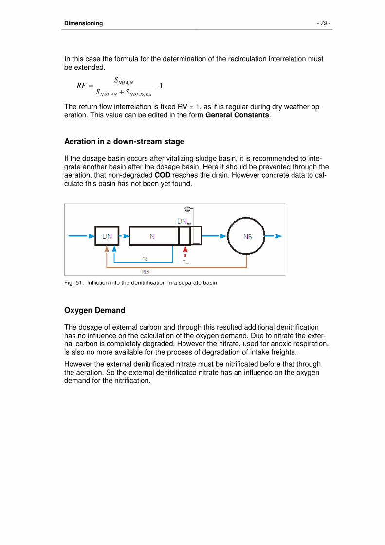
Dimensioning - 79 -
In this case the formula for the determination of the recirculation interrelation must be extended.
1,,3,3
,4−
+=
ExtDNOANNO
NNH
SS
SRF
The return flow interrelation is fixed RV = 1, as it is regular during dry weather op-eration. This value can be edited in the form General Constants.
Aeration in a down-stream stage
If the dosage basin occurs after vitalizing sludge basin, it is recommended to inte-grate another basin after the dosage basin. Here it should be prevented through the aeration, that non-degraded COD reaches the drain. However concrete data to cal-culate this basin has not been yet found.
Fig. 51: Infliction into the denitrification in a separate basin
Oxygen Demand
The dosage of external carbon and through this resulted additional denitrification has no influence on the calculation of the oxygen demand. Due to nitrate the exter-nal carbon is completely degraded. However the nitrate, used for anoxic respiration, is also no more available for the process of degradation of intake freights.
However the external denitrificated nitrate must be nitrificated before that through the aeration. So the external denitrificated nitrate has an influence on the oxygen demand for the nitrification.
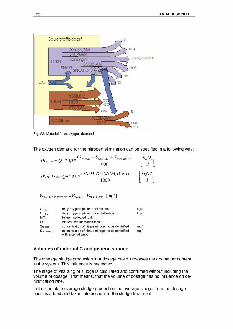
- 80 - AQUA DESIGNER
Fig. 52: Material flows oxygen demand
The oxygen demand for the nitrogen elimination can be specified in a following way:
+−=
d
kgOSSSQOU ESTNOIATNODNO
dNd2,3,3,3
,1000
)(*3,4*
−−=
d
kgOextDSNODSNOQdDOVd
2
1000
),,3,3(*9,2*,
SNO3,D,denitrificable = SNO3,D –SNO3,D,ext [mg/l]
OUd,N daily oxygen uptake for nitrifikation kg/d OUd,D daily oxygen uptake for denitrifikation kg/d IAT influent activated tank EST effluent sedimentation tank SNO3,D concentration of nitrate nitrogen to be denitrified mg/l SNO3,D,ext concentration of nitrate nitrogen to be denitrified
with external carbon
mg/l
Volumes of external C and general volume
The overage sludge production in a dosage basin increases the dry matter content in the system. This influence is neglected.
The stage of vitalizing of sludge is calculated and confirmed without including the volume of dosage. That means, that the volume of dosage has no influence on de-nitrification rate.
In the complete overage sludge production the overage sludge from the dosage basin is added and taken into account in the sludge treatment.

Dimensioning - 81 -
Basic Data
In the computation form for Basic Data the data for the dimensioning of the acti-vated sludge tank and secondary sedimentation tank are entered. The dimensioning includes the technical equipment as well ex. for mixing and aeration.
The clarifying processes of denitrification and phosphorus precipitation are at your choice. They are selected by clicking on the respective control box.
Fig. 53: Basic data without selecting denitrification or phosphorus removal (A126)
Organic Load and Sludge Volume Index
In the A131 and A126 guidelines different preselections are given for the organic load in the influent of the activated sludge tank.
Depending on the BOD5 concentration in the influent or the fraction of the organic trade load ,respectively, values for the sludge volume index (ISV) are preselected in both guidelines. These values may be adapted to individual requirements by the user.
The sludge volume index is a measure for the settleability of the activated sludge in the secondary sedimentation tank. The lower the ISV the better the settleability and the smaller the volume requirements for the secondary sedimentation tank. In other words, the higher the load, the larger the dimensions for the secondary sedi-mentation tank.

- 82 - AQUA DESIGNER
Technical Information: The Sludge Volume Index is a measure for the settleability of the activated sludge in the secondary sedimentation tank. It determines the volume of an unit of solid matter settling within a fixed time in a settling cylinder. Therefore, a high value for the sludge volume index means a delayed settling of the sludge. A sludge volume index of 80 - 100 ml/g characterises a sludge with good settleabil-ity. For activated sludge plants with the common municipal influent, and aerobic sludge stabilisation a ISV of 100 ml/g can be postulated for the dimensioning. High loads and high concentrations of biologically degradable organic substances in the influent cause a delay in settling or a higher sludge volume index , respec-tively. The upper limit for the required ISV is recommended by the A131 guideline (4.2.1 Anwendungsgrenzen und Abflußbeschaffenheit) as ISV <= 180 ml/g. Adding precipitants or flocculants in the form of iron or aluminium salts improves the settleability.
A131
In the option fields you may select a low or a high organic load for wastewater loading. The sludge volume index (ISV) is preselected depending on the selection and in accordance with the A131 guidelines.
Wastewater with ISV ml/g
low organic load 75 - 100 high organic load 100 - 150 Table: ISV and influent conditions
A126
In the option fields you may select loads with low, high or high and varying or-ganic load.
The value for the Sludge Volume Index (ISV) is preselected in accordance with the ATV guideline. In contrast to the A131 guideline, and depending on the amount of loading values for the mixed liquor suspended solids MLSS, concentration values in the activated sludge tank (SSAT) and values for volume loading (BR) are recom-mended here. The sludge load (BSS,BOD) results from these data.
Wastewater with ISV
g
ml
BSS,BOD
(F/M)
d*kg
kg
SSAT
(MLSS)
³m
kg
BR,BOD
d*m³
kg
low organic load 75 - 100 <= 0,05 <= 5 <= 0,25
high organic load 100 - 150 <= 0,05 <= 4 <= 0,20
high and extremely varying organic load
150 - 200 <= 0,05 <= 3 <= 0,15
Table: Organic Load (A126)

Dimensioning - 83 -
MLSS-Concentration / Sludge Tank
The volumes for the activated sludge tank and the secondary sedimentation tank are greatly influenced by the mixed liquor suspended solids concentration (SS-concentration) in the activated sludge tank.
Technical Information The SS(MLSS)-Concentration demonstrates the correlation between the activated sludge tank and the secondary sedimentation tank: To reduce the activated sludge tank volume it is possible to increase the SSAT. However this results in a larger surface area for the secondary sedimentation tank (or additionally to a deeper secondary sedimentation tank in the A131 respectively). On the other hand a larger volume for the activated sludge tank must be selected if the secondary sedimentation tank has to be designed to be smaller.
The mixed liquor suspended solids concentration SSAT value should not exceed 5 kg/m³ in the activated sludge tank.
A mixed liquor suspended solids concentration SSAT of < 2,5 kg/m³ should be cho-sen in the event of a high sludge volume index, or when the sludge settles with diffi-culties (ATV A131, 4.1.3).
A131
A value of 4,0 kg/m³ for the MLSS-concentration in the activated sludge tank is pre-selected based on the A131.
The ATV recommends the following values:
Standard of Purification SSAT (kg/m³) without pretreatment
With Nitrification (and Denitrification)
3,5 - 4,5
Sludge stabilisation (digestion) 4,0 - 5,0 Phosphorus removal (simultaneous precipitation)
4,0 - 5,0
Table: TS-Concentration in the activated sludge tank
A126
In contrast to the A131, the mixed liquor suspended solids concentration, in the ac-tivated sludge tank (SSAT) for the A126 guideline, is preselected depending on the amount of organic loading (Compare with the chapter ‘Organic Loading’).
- 84 - AQUA DESIGNER
MLSS-Concentration / Influent
The filterable solids or mixed liquor suspended solids in the inflow to the activated chamber are named SSo. For wastewater plants without pre-treatment step values for raw water must be entered.
A131
The mixed liquor suspended solids concentration (MLSS-Concentration) in the in-fluent for the activated sludge tank effects the sludge load and the sludge age.
The higher the SS-Concentration in the influent, the lower the sludge load. This re-sults in a larger volume for the activated sludge tank with an increase of SS-Concentration in the influent.
An increase of SS-Concentration in the influent increases the excess sludge pro-duction and , therefore, the sludge age decreases.
The absolute load of mixed liquor suspended solids is calculated with the above specific value and the municipal population equivalent. No specific SSo value is suggested for trade or industrial wastewater inflow. The specific SSo value must be adapted for including industrial or trade wastewater when their SSo is known. Devide the total SSo load by the municipal PE to obtain the new specific value. En-ter this value in the field SSo, Inflow Biological Chamber.
A126
The true MLSS-Concentration in the influent is not taken into account for the di-mensioning of the wastewater plant based on the A126 guideline. Therefore no in-put field appears. Compared to the A131, a simplified calculation is used for calculating the sludge load. The sludge age is not required for the dimensioning.
Sludge Age and Excess Sludge
Sludge Age
A131
Sludge Age for Denitrification, see Nitrification and Denitrification page 57.
The dimensioning of the activated sludge tank, in accordance with the ATV A131 guideline, is based on the sludge age in the AQUA DESIGNER Program.
Sludge load, volumetric loading and the required tank volume are calculated after choosing sludge age and TS-concentration in the influent and the activated sludge tank.

Dimensioning - 85 -
A sludge age of 25 d is recommended for the simultaneous aerobic sludge stabilisa-tion method to secure a sludge stabilisation in temperatures of 10°C. Different op-erators, however, consider a sludge age of 20 d sufficient enough, occasionally accepting only partial stabilisation of the sludge during winter months.
Plant Layout Standard of Purification up to
20.000 PT over
100.000 PT Wastewater treat-ment with Nitrifica-tion, Denitrification and Sludge stabili-sation
25
not
recommended
Table: Sludge age from ATV A131, Table 2
A126
A calculation based on the sludge age is not required.
Biological Excess Sludge Production
A131, 2000
For the biological waste sludge production WSBOD :
( )][
**17,01
**75,0*17,0*2,01*6,075,0
5,
,
,kgBOD
kgTS
Ft
Ft
C
XWS
TSS
TSS
IATBOD
IATSS
Cd+
−−+=
Basis COD
XWS = Xinert,IAT + XBM + Xinert,BM [mg/l]
XBM = Cdeg * Y – XBM * tSS * b * FT [mg/l]
+=
l
mg
FtbYCX
TSS
BM**1
1**deg
Inert solids from endogeneous degradation:
Xinert,BM = 0,2 * XBM * tSS * b * FT

- 86 - AQUA DESIGNER
International: Deutsch:
FT Temperature factor FT Temperaturabhängiger Fak-tor
-
tSS,min Sludge age (Input value) tTSmin Schlammalter (Eingabewert) d
Y Yield Y = 0,67 Ertragsfaktor gCSB/gCSBabb
b Degradation coefficient b = 0,17 Zerfallskoeffizient (T=15°C) 1/d
Cdeg Biodegradable COD Cabb,ZB Abbaubarer CSB mg/l
XBM COD-Konzentration of the biomass
XBM Als CSB gemessene Kon-zentration der Biomasse, bezogen auf Qt
mg/l
Xinert Concentration of inert COD
Xinert,BM Inerte Feststoffe aus endo-genem Zerfall der Biomasse
mg/l
XWS Concentration of excess sludge as COD
XÜS Als CSB gemessene Kon-zentration des Über-schußschlammes
mg/l
Xi-
nert,IAT Inert partikular COD (influent of the activated tank)
Xinert,ZB Inerter Anteil des partikulären CSB
mg/l
The total excess sludge production (WSB) results from the biological excess sludge and the ‘chemical’ excess sludge from phosphorus precipitation. (see the Chapters ‘Chemical Excess Sludge Production’ and ‘Total Excess Sludge Production’).
A126
Based on the A126 guideline a fixed value is postulated for the biological excess sludge production:
5
5 1kgBOD
kgSSWS BOD =
Sludge and Volume Load
A131
The sludge load results from the total waste sludge production (WSB) and the se-lected minimum sludge age (tSS,min):
=
dkg
kg
tWS SSB **
1 BSS
min,
The volume load (BR) results from the selected dry solids concentration in the acti-vated sludge tank (SSAT) and from the sludge loading rate (BSS).
=
dm
kg
*³SS * B B ATSSR
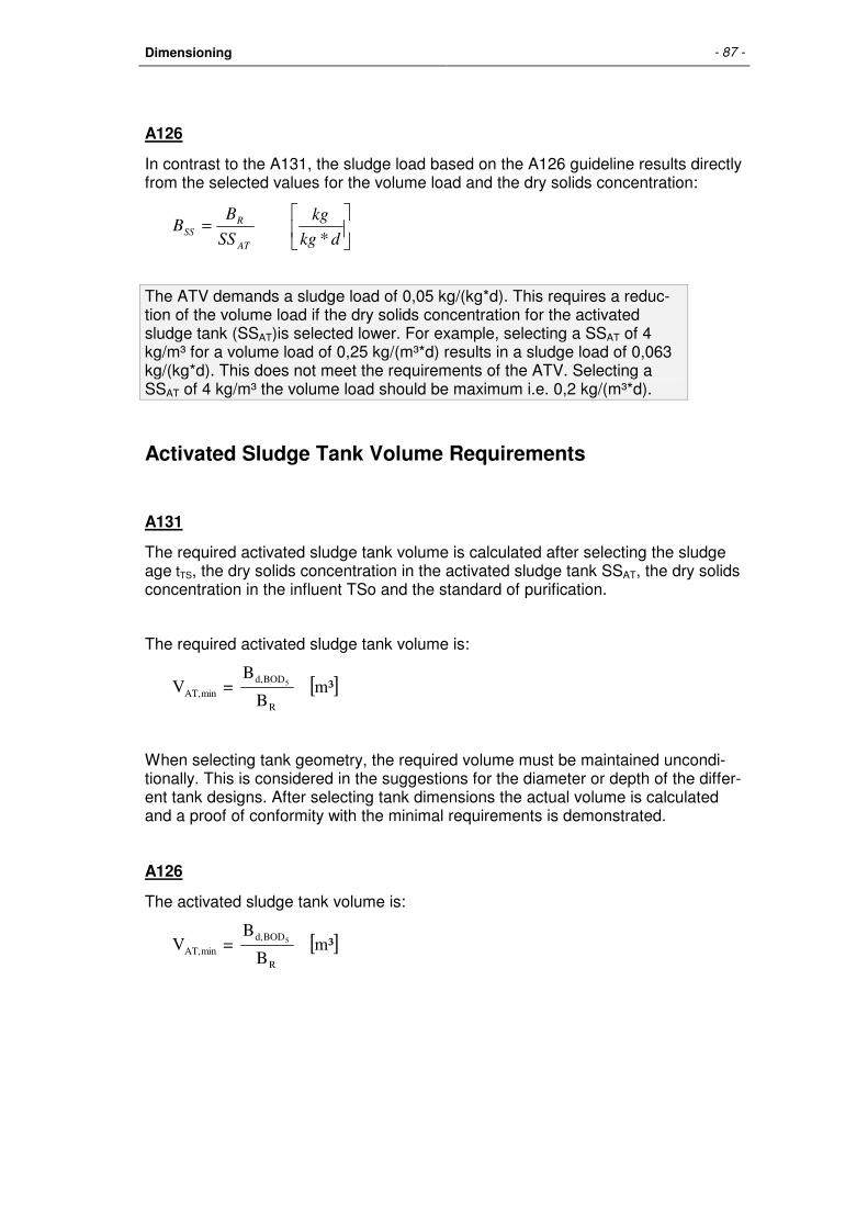
Dimensioning - 87 -
A126
In contrast to the A131, the sludge load based on the A126 guideline results directly from the selected values for the volume load and the dry solids concentration:
=
dkg
kg
SS
BB
AT
RSS
*
The ATV demands a sludge load of 0,05 kg/(kg*d). This requires a reduc-tion of the volume load if the dry solids concentration for the activated sludge tank (SSAT)is selected lower. For example, selecting a SSAT of 4 kg/m³ for a volume load of 0,25 kg/(m³*d) results in a sludge load of 0,063 kg/(kg*d). This does not meet the requirements of the ATV. Selecting a SSAT of 4 kg/m³ the volume load should be maximum i.e. 0,2 kg/(m³*d).
Activated Sludge Tank Volume Requirements
A131
The required activated sludge tank volume is calculated after selecting the sludge age tTS, the dry solids concentration in the activated sludge tank SSAT, the dry solids concentration in the influent TSo and the standard of purification.
The required activated sludge tank volume is:
[ ]m³ B
B = V
R
BODd,
minAT,
5
When selecting tank geometry, the required volume must be maintained uncondi-tionally. This is considered in the suggestions for the diameter or depth of the differ-ent tank designs. After selecting tank dimensions the actual volume is calculated and a proof of conformity with the minimal requirements is demonstrated.
A126
The activated sludge tank volume is:
[ ]m³ B
B = V
R
BODd,
minAT,
5

- 88 - AQUA DESIGNER
Return Sludge Ratio
A131
The return sludge ratio (RS) is included in the dimensioning of the activated sludge tank within the calculation step for different depths. The return sludge ratio is se-lected by the user and determines the ratio between the MLSS-concentration in the activated sludge tank and in the return sludge.
ATRS
AT
SSSS
SSRS
−=
The selection of a transport unit in the form Return Sludge Transport is based on the values entered in the form Basic Data.
The ATV report:„Anwendungshinweise zum ATV-Arbeitsblatt A131 – Teil Nachklär-becken” /7/ advises return sludge ratio limits under different hydraulic conditions.
A maximum return sludge ratio of 0.75 * Qstormwater is advised for the dimensioning of secondary sedimentation and activated sludge tank in the selection of the horizontal flow secondary sedimentation tank. The machines for return sludge transport should be set for a capacity of 1.0 * Qstormwater for the operation.
A maximum ratio of 1.0 * Qstormwater for the dimensioning with the vertical flow sedi-mentation tank is recommended in the above mentioned report. The capacity of the transport machinery should cover 1.5 * Qstormwater for operation.
The ATV recommends Qdryweather values as well. The basic value for the horizon-tal flow sedimentation tank is recommended as 1.5 * Qdryweather; and for the vertical flow sedimentation tank a maximum return sludge ratio of 2.0 * Qdryweather is recom-mended.
AQUA DESIGNER reviews the input data and indicates when limiting values are exceeded. The Software also examines whether a selected return ratio for Qm with combined wastewater inflow and stormwater is within limits for the dry weather con-dition as well. If this is not the case AQUA DESIGNER will point this out with a hint. In any case it is possible to continue the calculation with the selected values and conditions.
A126
In contrast to the A131 guideline the return sludge ratio is not considered in the di-mensioning of the secondary sedimentation tank based on the A126 guideline.
The selection of the transport unit for the return sludge transportation is based on the return sludge ratio.

Dimensioning - 89 -
Nitrification
Sludge Age for Nitrification, see Only Nitrification page 56.
The sludge age is sufficient for the nitrification process in activated sludge plants designed for aerobic sludge stabilisation. Therefore nitrification continuously takes place if satisfactory aeration is guaranteed.
The ATV guidelines demand a measuring/operating/ process design temperature of 10°C.
This value may be accessed and adapted in the list of details under Options > De-tails.
Denitrification
Sludge Age for Denitrification, see Nitrification and Denitrification page 57.
Denitrification may be selected in the menu under Options > System of Nutrient Elimination.
Denitrification is treated differently by the A131 and A126 guidelines which affects the aeration.
A131
The oxygen requirement and the aeration period are affected when Denitrification is selected. These values are later suggested in the window Aeration.
An input field Nitrate-N in Effluent (Ne) appears with a preselected value for the nitrate nitrogen in the effluent (NO3-N mg/l). The same applies to the Ammonia-N in Effluent (NH4-N)e.
From the nitrate nitrogen in the effluent the nitrogen load for denitrification is com-puted. The value for the nitrate-N is preselected as 3 mg/l, ammonia nitrogen in the effluent is selected as NH4-N = 1 mg/l.

- 90 - AQUA DESIGNER
Fig. 54: Basic data based on ATV A131 with denitrification
The nitrogen balance is calculated using the ammonia NH4-N concentration in the influent and outflow, and the Nitrate NO3-N concentration in the outflow. The result gives the values for nitrificated and denitrificated nitrogen.
The ammonia concentration in the influent corresponds with the nitrogen load en-tered into the form Load. The values in the input fields for ammonia nitrogen and nitrate nitrogen in the outflow are suggestions representing the recommended de-gree of purification.
A fraction of 0.04 - 0.05 kg nutrient per kg BOD5 is used by the micro-organism me-tabolism and incorporated into the biomass. This fraction is removed from the sys-tem with the excess sludge and, thus, is not included in the computation for the nitrification/denitrification or the nitrogen balance.
The fraction of incorporated nitrogen may be accessed in the list of details under options > details. The value may be changed in this list.
Design for nitrogen removal (nitrogen loads in kg/d)
Nbio = fNbio * Nzu [kg/d]
NNitri = Nzu - Nbio [kg/d]
NDeni = Nzu - Nbio - Nab [kg/d]
Here the design differs from the ATV guideline. According to the ATV conventions it is:
Nab = NO3-Ne (ATV) and NDeni = NO3-ND (ATV) [mg/l]

Dimensioning - 91 -
A131, 2000
SNO3,D = CN,ZB–Corg,AN–SNH4,AN–SNO3,AN–XorgN,ÜS [mg/l]
Technical Information Denitrification processes in the activated sludge tank result in different positive effects.
In the nitrification oxygen is used for the oxidation of ammonia to nitrate. In the denitrification part of the used oxygen is again utilised by the heterotro-phic bacteria. This has a positive effect on the total oxygen requirements in the nitrogen removal process provided by aeration. The operating costs for aeration are reduced with reduced oxygen re-quirements. However, it should be noted that lower oxygen requirements have to be transferred in a shorter time period with reduced aeration peri-ods. This leads to higher investment costs for the aeration system which, however, generally does not invalidate the positive effect of the reduction in operating costs.
In the nitrification H+-Ions are released. This reduces the buffer capacity of the wastewater. In the denitrification this process is partly reversed through binding of H+-Ions. This has a positive effect on the pH value and, thus, the process stability.
Decisive for the success of the denitrification and biological phosphorus removal is the TKN/BOD5-Ratio in the activated sludge tank influent. It is important to ensure that the complete BOD5 of the influent is available for the above mentioned processes if the ratio is too large, ex. larger than 0,2. /13/ These cases should be computed without the primary sedimentation or with a shorter primary step respectively as in the here available processes.
It should be noted that the intermittent denitrification is disadvantageous, as carbon compounds are degraded in the aerobic phase that are not available in the anoxic phase.
You will find further information about denitrification in the part on aeration and oxy-gen requirement.
A126
In the computation based on the A126 guideline no value for the nitrate in the efflu-ent is required and thus, there is no nitrate nitrogen balance.
In contrast to the A131 guideline the choice of Denitrification only has an effect on the aeration period.
The aeration period is preselected as 16 h/d in the form Aeration. During the 8 hour anoxic phase denitrification takes place.
The separate mixing and aeration option is preselected choosing denitrification.
Mixing devices are required that maintain circulation during the denitrifica-tion period without aeration.
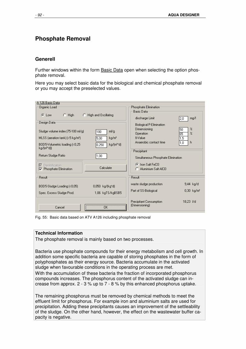
- 92 - AQUA DESIGNER
Phosphate Removal
Generell
Further windows within the form Basic Data open when selecting the option phos-phate removal.
Here you may select basic data for the biological and chemical phosphate removal or you may accept the preselected values.
Fig. 55: Basic data based on ATV A126 including phosphate removal
Technical Information The phosphate removal is mainly based on two processes. Bacteria use phosphate compounds for their energy metabolism and cell growth. In addition some specific bacteria are capable of storing phosphates in the form of polyphosphates as their energy source. Bacteria accumulate in the activated sludge when favourable conditions in the operating process are met. With the accumulation of these bacteria the fraction of incorporated phosphorus compounds increases. The phosphorus content of the activated sludge can in-crease from approx. 2 - 3 % up to 7 - 8 % by this enhanced phosphorus uptake. The remaining phosphorus must be removed by chemical methods to meet the effluent limit for phosphorus. For example iron and aluminium salts are used for precipitation. Adding these precipitants causes an improvement of the settleability of the sludge. On the other hand, however, the effect on the wastewater buffer ca-pacity is negative.

Dimensioning - 93 -
An effluent limit of 2 mg/l can be met during the summer months with solely bio-logical phosphorus removal as operating experiences with one step activated sludge plants show. The biological phosphorus removal is dependent on the wastewater contents, the sludge load and the selected clarification method. Intermittent denitrification is use-ful for the biological phosphorus removal with almost anaerobic conditions present towards the end of the Deni-phase. This stress situation favours bacteria with en-hanced phosphorus uptake to accumulate in the activated sludge. A high concentration of easily biodegradable organic compounds improves the bio-logical phosphorus removal. The efficiency for the biological phosphorus removal reduces during the winter months in that a chemical precipitation should be considered for keeping the limit of 2 mg/l. Metal salts are mainly used as precipitants. The solute metal ions together with the solute phosphorus compounds form an insoluble compound precipitating as flocs in the activated sludge. The addition of metal ions has a negative effect on the wastewater buffer capacity as H+-Ions are released with the formation of the metal phosphate complex. Formation of metal phosphate Me3+ + H2PO4
- � MePO4 + 2 H+ Formation of metal hydroxide Me3+ + 3 H2O � Me(OH)3 + 3 H+
Fig. 56: Possible points of application in the simultaneous precipitation

- 94 - AQUA DESIGNER
Biological Removal
Part of the phosphorus load in the influent is degraded by micro-organism. The theoretical foundation is discussed earlier in the part on degradation of phosphorus compounds.
The fraction of the biologically removed phosphorus load from the total phosphorus load in the influent is preselected with different values in two input fields of the form Basic Data: The biologically removed fraction is selected lower for the precipitation than for the estimate of the operation costs. This is on the one hand necessary to secure the phosphate precipitation in the winter period and on the other hand to only calculate with the average consumption for the operating cost.
The excess sludge from biological phosphorus removal may be disregarded for the A131 guideline.
Fig. 57: Example: Phoredox-System; (AB = anerobic tank, DN = denitrification zone, N = nitrifikation zone, NB = sedimentation tank)
The required anaerobic volume is dimensioned in accordance with the recommen-dations given by Boll /1/. The suggested period of contact in the input field for An-aerobic contact period is related to the influent and the return sludge. Further information is available in the chapter on ‘Theoretical Foundations’.
Chemical Removal
The ß-value is the molar ratio of the amount of added iron or aluminium ions ex-ceeding the stoichiometrically required value. It represents the ATV A202 recom-mendations and its methods for elimination of phosphorus from the wastewater (ATV A202, Verfahren zur Elimination von Phosphor aus Abwasser).
From Table 1 of the ATV A202 guideline the most frequently used precipitants were selected that are aluminium chloride AlCl3 and iron(III)-chloride FeCl3
.6H2O.
Both precipitants are presumed as 40-% solutions.
Chemical Form of Supply Effective Ion Dosage for ß = 1,5
AlCl3 approx. 40-% Solution
Al3+ 65 mg/l AlCl3
FeCl3.6H2O approx. 40-%
Solution Fe3+ 79 mg/l
Extract from Table 1: Precipitants; ATV-A202

Dimensioning - 95 -
The method of choice is the simultaneous precipitation.. In this method the precipi-tant is directly added to the biological step. The point of application for the precipi-tant is the biological reactor or the return sludge pump station. An adequate mixing of the liquor with the precipitant is essential.
The Concentration of precipitant and the specific weight can be edited in Options > General Constants in the register Sludge Treatment/Precipitants.
Precipitant Requirement
The precipitant requirement results from the molar ratio ß for the addition and the composition of the precipitant.
Ratio of the atomic masses of iron and phosphorus:
1,8 = 30,97
55,85 =
M
M
P
Fe
0,87 = 30,97
27,00 =
M
M
P
Al
MFe Atomic mass iron [g/mol] MAl Atomic mass aluminium [g/mol]
The added metal mass results for ß = 1,5 to:
salt aluminiumfor gAl/gP 1,3
saltiron for gFe/gP 2,7*
=
=ßM
M
P
Chemical Waste Sludge Production
Additional excess sludge results from the phosphate precipitation and is included into the computation for the dimensioning of the activated sludge tank based on the A131 guideline. Depending on the nature of the precipitant different chemical ex-cess sludge productions result.
For precipitation with iron salt:
5BODd,
elim
PkgBOD
kgSS
B
P * 6,8 =
5
WS
For precipitation with aluminium salt:
5BODd,
elim
PkgBOD
kgSS
B
P * 5,3 =
5
WS
WSP sludge production from chemical phosphorus re-moval
kg/kg
Pelim P-load for removal (elimination) [kg/d] Bd,BOD5 BOD5-Influent [kg/d]
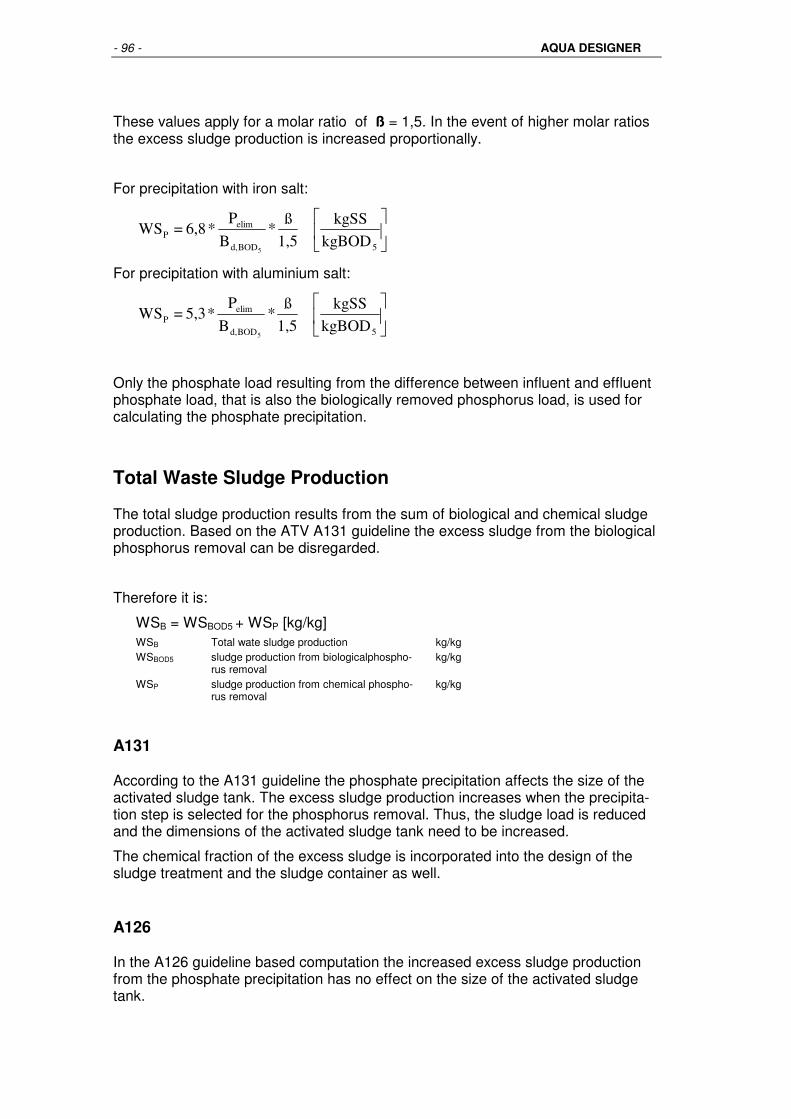
- 96 - AQUA DESIGNER
These values apply for a molar ratio of ß = 1,5. In the event of higher molar ratios the excess sludge production is increased proportionally.
For precipitation with iron salt:
5BODd,
elim
PkgBOD
kgSS
1,5
ß *
B
P * 6,8 = WS
5
For precipitation with aluminium salt:
5BODd,
elim
PkgBOD
kgSS
1,5
ß *
B
P * 5,3 = WS
5
Only the phosphate load resulting from the difference between influent and effluent phosphate load, that is also the biologically removed phosphorus load, is used for calculating the phosphate precipitation.
Total Waste Sludge Production
The total sludge production results from the sum of biological and chemical sludge production. Based on the ATV A131 guideline the excess sludge from the biological phosphorus removal can be disregarded.
Therefore it is:
WSB = WSBOD5 + WSP [kg/kg] WSB Total wate sludge production kg/kg WSBOD5 sludge production from biologicalphospho-
rus removal kg/kg
WSP sludge production from chemical phospho-rus removal
kg/kg
A131
According to the A131 guideline the phosphate precipitation affects the size of the activated sludge tank. The excess sludge production increases when the precipita-tion step is selected for the phosphorus removal. Thus, the sludge load is reduced and the dimensions of the activated sludge tank need to be increased.
The chemical fraction of the excess sludge is incorporated into the design of the sludge treatment and the sludge container as well.
A126
In the A126 guideline based computation the increased excess sludge production from the phosphate precipitation has no effect on the size of the activated sludge tank.

Dimensioning - 97 -
BOD5-Degradation
The degradation of BOD5 is determined by degree of degradation and sludge load-ing.
Fig. 58: BOD5 degradation (BSB5-Abbau) depending on sludge loading (Schlammbelastung)
The sludge age ofdimensioning by AQUA DESIGNER is between 3 and 25 days. This means a BOD5 degradation of 92-93 %.

- 98 - AQUA DESIGNER
University Algorythm
In 1988 a work group was constituted that in following developed a dimensioning method as a basis for computation models. This dimensioning method resulted from the exchange of exprience of 11 universities and since has been modified and adapted to practical experience. The University Algorythm and the ATV guideline A131 fundamentally have the same basis.
The dimensioning approach was published in 1989. A supplement was published in 1993 when particularly some constant values were modified.
Additionally to the ATV dimensioning guidelines the university algorythm is an im-portant tool for the dimensioning of activated sludge waste water clarification sys-tems. The university algorythm offers the oppertunity to compute outflow values on the basis of kinetic laws. It therefore offers superior results.
The university algorythm suggests differing partly lower volumes in certain condi-tions. Here a comparitive computation is useful for economic reasons.
The AQUA DESIGNER dimensioning is primarily based on the following publica-tions:
• Dimensioning of nitrogen elimination in the wastewater plant 8/89 /19/
• Dimensioning of wastewater plants for nitrogen elimination, compare ATV A131- HSG 2/91 /20/
• Dimensioning of activated sludge tanks based on the university algorythm -HSG-Ansatz- 8/93 /21/
Fig. 59: Primary data based on the university algorythm considering phosphate removal and without simultanous aerobic sludge stabilization

Dimensioning - 99 -
Scope
The university algorythm is applicable for single and multistage wastewater plants with domestic wastewater or wastewater comparable to domestic wastewater.
Wastewater plants for limits of NH4-N lower than 3 mg/l can not be dimensioned.
The calculated nitrate outflow values are average operating values. Limits for the nitrate outflow concentrations can not be obtained from the university algorythm.
Variation of Method
The below listed variations of method may be selected from the menu bar with Op-tions > Process for nitrogen removal. You may only select these methods from the Main Window level. You must begin the computation from the Basic Data form if a new method was selected.
Fig. 60: Selecting a method for nitrogen removal from the menu bar
Nitrification
The aerobic sludge age equals the total sludge age when only nitrification was se-lected. The aeration period is suggested as 24 hours. The nitrate outflow concentra-tion appears as result of the computation.
Intermittant Denitrification
The daily aeration period equals the ratio of nitrification volume to total volume. As the actual aeration takes place over a shorter period it must be adapted accordingly and designed larger in the dimensioning. Mixing devices are required when select-ing compressed air aeration to keep the activated sludge in suspension during the aeration free period and to obtain a satisfactory mixture.

- 100 - AQUA DESIGNER
Combined Nitrification / Denitrification
The aeration period is suggested as 24 hours. The mixing devices are only dimen-sioned for the denitrification tank volume. One mixing device is suggested per line. More devices must be selected accordingly if multiple denitrification tanks are con-structed in one line. The required recirculation energy will automatically be included in the calculation for the operation costs.
Simultaneous Denitrification
The aeration period is 24 hours. Mixing devices are required for compressed air aeration to maintain the circulation and keep the activated sludge in suspension also in the non-aerated sections. There is no increased initial respiration in the si-multaneous denitrificaion affecting the dimensioning. The factor of increased respi-ration a is equal to 1.
Inflow
The inflow data were previously entered into the form for Loads. These data are processed in the dimensioning based on the A131 guideline as well as based on the university algorythm.
In addition to the data for the form on Loads the following data are entered into the Basic Data form:
TS0 filterable particles in the inflow kg/PT/d
(NO3-N)0 Nitrate concentration in the inflow mg/l
TS0 is of great influence on the dimensioning and must be selected carefully. You will find the information on the TS0 value ranges in the dimensioning guideline for the A131.
Outflow Requirements
The outflow limits for nitrogen and phosphate are entered into the Basic Data form. The dimensioning of nitrogen removal is based on its peak values and average val-ues.
Preselected Values
Standard outflow values are preselected.
control limits daily peak value
daily average
Nanorg mg/l 18 I) 18 12 NH4-N mg/l 5 - 10 II) 5 - 10 1 - 2 NO3-N mg/l - - 10 I) ÜW Appendix 1; II) ÜW Appendix 1, 10 mg/l

Dimensioning - 101 -
The outflow concentration for organically bound nitrogen is 2 mg/l.
Calculated Values
Average outflow values may be calculated on the basis of the peak values. Click on the control box Outflow Values in the frame for Calculate Values to calculate the average values.
The input fields for the average ouflow values will disappear as they are calculated.
NH4-N median value in dimensioning = NH4-N peak value in dimensioning / 5
NO3-N = N anorg.(ÜW) / 1,5 - NH4-N (median value in dimensioning)
Calculative Algorythm
Aerobic Sludge Age
The daily fluctuation in the wastewater nitrogen load is considered in the dimension-ing by including a fluctuation factor. The above listed literature demands that a fluc-tuation factor should whenever possible be calculated from data obtained through measurement. These data should be obtained through the period of at least one sludge age.
Fluctuation factor:
24,4,
,4,
*)][(
*)][(
QNNHN
QNNHNS
memn
PPePn
−−
−−=
S Fluctuation factor Nn,P Nitificable peak ammonia inlet mg/l Nn,m Average (middle) nitificable ammonia inlet mg/l QP Inflow according to nitrificable nutrient con-
centration m³/h
Q24 24-hours average inflow m³/h
It is possible to calculate the fluctuation factor based on measurements when se-lecting the university algorythm computation in the Basic Data form.
Click on the control box for the Fluctuation Factor in the frame for Calculate Val-ues. Input fields for nitrogen inflow peak values and correspondent wastewater vol-umes will appear.
The fluctuation factor is fixed in accordance with the university algorythm in the case of no available measurement data and no specified data entered into the pro-gram.
The following values are applied in the case of no available measurement data:
Population equivalent of < 20000 PT: S = 2,0
Population equivalent of >= 20000 PT: S = 1,7

- 102 - AQUA DESIGNER
The theoretical sludge age is calculated based on the work of Monod on ammonium outflow concentration and rate of growth of nitrate bacteria. The influence of tem-perature is considered by the use modifying temperature factors.
The safety factor f' comprises operating effects like partially insufficient oxygen con-centration, fluctuating pH value or the effect of inhibiting factors on nitrate bacteria.
An adequate nitrification rate requires a minimum oxygen concentration of 0,5 mg/l in the overall nitrification volume. Therefore the aeration should be designed for 2 mgO2/l. This is considered in the dimensioning of the aeration system.
Theoretical aerobic sludge age requirement:
][
**][
][*
max
'
,,
,4
,4
, d
fbfNNHK
NNH
S
ft
bATAAT
PeN
PeASS
−−+
−=
µ
f’ safety factor - fT,A temperatur factor for autotrophic growth - fT,bA temperatur factor for autotrophic die rate - KN half life constant for Nmax mg/l bA die rate of autotrophic organismen 1/d µmax growth rate -
Excess Sludge Production
The excess sludge production is of major importance for dimensioning the biological step. Different processes and conditions affect the activated sludge composition and the excess sludge production.
The filterable particles found in the wastewater plant inflow are of great influence on the excess sludge production. It is important to enter a realistic value. Approximate values based on Böhnke, B. und Pinnekamp, J. may be entered in the case of no available measurement data. These approximations are used in the A131 guideline as well.
Type of wastewater plant
Typical Value of So
mg/l
Typical Value of TSo mg/l
TSo/So
Without primary treat-ment
300 360 1,2
With primary treatment 210 170 0,8 conv. 2-step 50 50 1,0 Adsorption-Step 150 50 0,33 Tab:Typical (Characteristic) values for So and Tso in the nitrification/dentrification step inflow depending on the primary treatment

Dimensioning - 103 -
Biomass in the Activated Sludge
The autotrophic microorganism are responsible for nitrification. The fraction of auto-trophic microorganism is primarily fixed by the aerobic sludge age.
Fraction of autotrophic microorganism:
+
−−=
³**1
**)][(*
,,
,,4,
m
kgSS
tfb
tqRNNHNyx
ASSbATA
totalSSmemnA
A
XA Part of autotrophic organismen in actvated sludge
-
YA Yield of autotrophic biomass mg/mg Nn,m Average (middle) nitificable ammonia inlet mg/l qR Volume loading m³/(m³*d) bA Die rate of autotrophic organismen 1/d fT,bA Temperatur factor for autotrophic die rate - tSS,A Aerobic sludge age d tSS,total Total sludge age d
The heterotrophic microorganism reduce the organic load and use the nitrate pro-duced in nitrification for the nitrate respiration. Thus, they are responsible for denitri-fication.
Fraction of heterotrophic microorganism:
+=
³**1
*'***
,,
,
m
kgSS
tfb
tqRSoyx
totalSSbHTH
totalSSH
H
η
XH part of heterotrophic organismen in actvated sludge
-
YH yield of heterotrophic biomass mg/mg η yield of BOD-degradation - So’ Inflow-BOD-concentration mg/l fT,bH temperature factor for heterotrophic die rate -
The inactive fraction of the activated sludge is composed of the inflowing load of filterable particles and the fraction of dead heterotrophic and autotrophic biomass.
Fraction of inactive particles :
+
+=
³****
*******
,,
,,,
m
kgSStxfbfi
txfbfitqRSSofx
ASSAbAtA
totalSSHbHTHtotalSSPI
fP Part of inert solids -
Fraction of precipitation sludge:
++=
³*)*9,2*9,1**5,1( ,
m
kgSStAlFeQPx GSSF

- 104 - AQUA DESIGNER
The phosphate precipitation increases the solids concentration in the activated sludge tank. AQUA DESIGNER always designs the activated sludge tank on the basis of the preselected solids concentration. In the case of phosphate precipitation the activated sludge xH+xA+xI fraction is reduced in steps until the dry solids concen-tration in the activated sludge tank including the precipitation sediment equals the preselected dry solids concentration.
When 3,75 kg/m³ was entered for MLSS in the activated sludge tank:
=+++=
³ 3,75 xxx x SS FHAIAT
m
kgSS
The total excess sludge is the sum of the above described and produced fraction of the activated sludge devided by the sludge age. This results from the definition of sludge age as the average detention time of the activated sludge.
Waste sludge production:
+++=
dm
kgSS
t
xxxxWS
totalSS
FIAHR
*³,
Buffer Capacity
The wastewater buffer capacity is reduced by different processes in the activated sludge tank. The effects of nitrification, denitrification and phosphate precipitation are discussed in detail in the chapter on the Theoretical Foundations.
The university algorythm defines the buffer capacity in the biological step outflow as follows.
Buffer capacity:
−++−
−−−+−+
−−=
l
mmolPePoAlFe
NeNONoNONeNH
NoNHSKoSKe
)(*03,0*03,0*06,0
)(*14
1
*14/1
334
4
Sko Buffer capacity in the biological step inflow

Dimensioning - 105 -
Respiration Increasing Factor
The respiratory activity in the denitrification tank is increased in the event of pre-set/preliminary denitrification because of concentrated substrate feed. The intermit-tant denitrification is treated like the preset/preliminary denitrification in the ATV131 guideline. Here as well an increased respiratory activity is taken into account. In the simultaneous denitrification the respiratory elevation factor is a=1.
Pre stage (RF <10), intermittant denitrification:
235,0
*100*95,2
−
=
V
Va D
Simultaneous denitrification:
a = 1
VN/V-Ratio Evaluation
The equations on the denitrificable Nd,m1 and the nitrogen to be denitrificated, Nd,m2, must result in the same sum to evaluate the VN/V-ratio.
The factor for increased respiration is incorporated into the equation for evaluating the oxidized nitrogen.
Denitrificable nitrogen:
+
+
=
l
mg
V
Vtfb
fV
VAty
V
VSo
faN
N
ASSbHTH
bHT
N
SSH
DDmd
***1
**,**24,0
5,0*
'***86,2
*
,,
,
1, η
Nd,m1 concentration of denitrificable nitrigen mg/l YH yield of heterotrophic biomass mg/mg η yield of BOD-degradation - So’ inflow-BOD-Concentration mg/l fT,bH temperature factor for heterotrophic die rate -
The fraction of incorporated nitrogen NÜS is included in the equation for evaluating the oxidized nitrogen. A factor for nitrogen return load is introduced as nitrogen from sludge storage and sludge treatment may return into the circulation with the turbid water. This factor rx has a standard value of 0 meaning that the nitrogen return load is primarily not considered.
The rx value may be adapted in the list of constant values under Options > Con-stant Values HSG if the nitrogen return load is to be considered.

- 106 - AQUA DESIGNER
Denitrificated nitrogen:
−−−−−−
++=
l
mgNÜSorgNeNNONNH
NFKNÜSrxmTKNoN
eme
md
][][
*,
3,4
2,
rx Fraction of nitrogen return load Standard value rx = 0
Nd,m2 Concentration of denitrificated nitrogen mg/l orgNe
Organic nitrogen in the outflow Standard value orgNe = 2 mg/l
mg/l
NFK Nitrogen from external sludge addition
The NFK fraction ist not treated separately in AQUA DESIGNER. The external sludge may be entered in the industriell sludge fraction in the Basic Data form.
Incorporated nitrogen fraction of the activated sludge:
++=
l
mg
qRt
xiixixiN
GSS
IABHBWS
*
***
,
Volume Load
The required volume is calculated from the Volume Load and the daily wastewater inflow. First the constant P is calculated for evaluating the Volume Load.
++
−−+
++
+
++
=
l
mgAlFe
NNHNyAtfbA
tfbAfi
SoyHtfbH
tfbHfi
TSofpP
memn
ATSbAT
ATSbAT
GSSbHT
GSSbHT
*0,4*5,2
)]4[(****1
***1
*****1
***1
*
,,
,,
,,
,,
,,η
=
dm
m
P
WSRqR
*³
³
Constant Values
The listed constant values are an internal part of the university algorythm. They should not be changed without significant reason as consequently the calculations will not follow the recommendations of the university algorythm anymore.
Exeptions are the fraction of phosphate in the activated sludge ip and the fraction of the nitrogen return load rx.

Dimensioning - 107 -
The fraction of phosphate in the activated sludge can be selected up to ip = 0,08 when biological phosphate removal is assumed or operationally enhanced.
f' 1,25 fD 0,75 fi 0,20 fT,A 1,103 fT,bA 1,090 fT,bH 1,073 fp 0,60
0,95 rx 0,55 bA 0,05 d-1 bH 0,17 d-1 iB 0,12 kgN/kgBiomas
s iI 0,01 kgN/kgTS ip 0,03 KN 0,70 mg/l nmax,A 0,52 d-1 YH 0,75 YA 0,15 B 0,12

- 108 - AQUA DESIGNER
Continuous Flowed ASS
Upstream Anaerobic Chamber
The theoretical basis will be found at Chapter “Biological Phosphate Elimination”
Choosing a Chamber
Its possible to integrate the anaerobic volume into the volume of the activated chamber. This is usefull for example together with the intermittend denitrification. The basics will be found in /10/. In an intermittend denitrification process you will have totally anaerobic conditions at the end of the denitrification phase. So you can extend the anaerated phase and add an anaerobic phase.
Choose Options > Process and in the frame Basis of Design A131 the Option Separate Stage Anaerobic Mix Tank.
Fig. 61: Options > Process: Selection of an upflow anaerobic mix tank
In the flow diagram a new field Anaerobic Mix Tank will occure.
If you have chosen an anaerobic mix tank, in Basic Data the Biological Phos-phate Elimination is presetted and cannot be deactivated.

Dimensioning - 109 -
Fig. 62: Biological P-elimination pre selected, in combination with upflow anaerobic chambe
Design of the Chamber
By the DWA A131 the retention time is the parameter for the design of the anaero-bic volume. Its recommend with 0,5 – 1,0 h. Please note that the retention time re-lates to inflow and return sludge flow.
³][mQQdw
tV
RS
RAC
+=
VAB Volume of the Anaerobic Chamber tR Retention Time
Fig. 63: Design upstream anaerobic mix tank
Rectangular and circular chambers are available. Typical or suitable values are al-ways presetted.

- 110 - AQUA DESIGNER
If you want to select more than one line, go to Options and enter the number of lines for the anaerobic chamber. Its also possible to define the mixing devices by pushing the button Mixing.
Upflow Aerobic Selector
In case to prevent the grow of filamentous bacteria it proved effectively to integrate an upflow aerobic selector as a high loaded fermenter before the activated cham-ber. The upflow high loaded reactor inhibits the growth of filamentous bacteria and so the growth of bulking sludge /31/.
In the selector air will be injected. This will however not effect to the aeration of the biological chamber. As the infected oxygen will be totally used up here, there will be no negativ effect to a following denitrification. As there is no definitely declaration whether the oxygen supported to the selector can be deducted from the oxygen demand in the activated chamber, the designer can decide this for himself in Aqua Designer.
Varations of Aeration
Fig. 64: Variations of the aration of selector and activated chamber
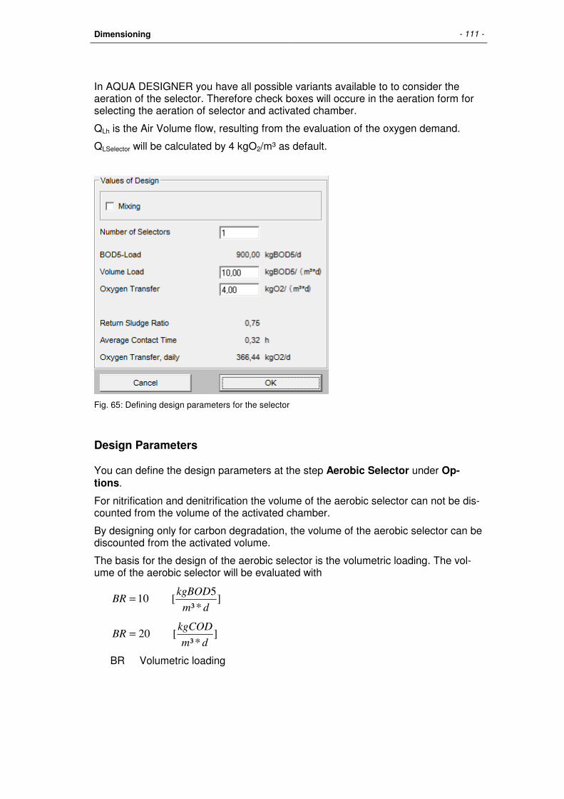
Dimensioning - 111 -
In AQUA DESIGNER you have all possible variants available to to consider the aeration of the selector. Therefore check boxes will occure in the aeration form for selecting the aeration of selector and activated chamber.
QLh is the Air Volume flow, resulting from the evaluation of the oxygen demand.
QLSelector will be calculated by 4 kgO2/m³ as default.
Fig. 65: Defining design parameters for the selector
Design Parameters
You can define the design parameters at the step Aerobic Selector under Op-tions.
For nitrification and denitrification the volume of the aerobic selector can not be dis-counted from the volume of the activated chamber.
By designing only for carbon degradation, the volume of the aerobic selector can be discounted from the activated volume.
The basis for the design of the aerobic selector is the volumetric loading. The vol-ume of the aerobic selector will be evaluated with
]*³
5[10
dm
kgBODBR =
]*³
[20dm
kgCODBR =
BR Volumetric loading

- 112 - AQUA DESIGNER
The volume is:
³][10
BV
BOD5d;
BOD5AS, m=
³][20
BV
CODd;
CODAS, m=
The oxygen input should be:
]*_³
2[4
dVolumeChamberm
kgOOC =α
Mixing Device
To include the mixer for the selector, activate the check box Mixing in the form Val-ues of Design. By leaving the active form Values of Design you will come back to the main formular for the selector. Now a button Mixing is visible.
Here you can select the mixer or a number of mixers out of the Data Bank.
Fig. 66: Selecting mixers for the selector
If you have chosen more than one selectors, here the number of mixers means one chamber.
By clicking OK you come back to the flow diagram.

Dimensioning - 113 -
Secondary Sedimentation Tank
Design Variations
The particular advantage of AQUA DESIGNER is the opportunity of selecting a va-riety of different sedimentation chambers. You may select vertical or horizontal flow sedimentation chambers, hopper-bottom tanks and tanks with flat bottom, rectangu-lar tanks or circular tanks. It is possible to calculate chambers in parallel and com-pare them while calculating. Through these features you are enabled to determine the most economical solution.
Several different designs for secondary sedimentation tanks are available to you.
ATV Guideline: A 126 A 131
Methods: horizontal flow vertical flow
Construction styles: Chambers with flat bottom and slope (Plate remover or Sludge scrapers) Chambers with flat bottom without slope (Suction remover) Hopper-Bottom Tanks Circular Tanks Rectangular Tanks
The vertical flow or upward flow secondary sedimentation tank is available as hop-per-bottom tank construction with the following advantages: Moveable mechanical equipment for sludge removal is not required, and there is a more effective sedi-mentation than in the horizontal-flow tank with an even base.
Fig. 67: Main Window with available choices for secondary sedimentation tanks

- 114 - AQUA DESIGNER
Depending on the conditions of the ground and ground water, however, hopper-bottom tanks are only constructed economically up to a limited hydraulic load.
Horizontal-flow tanks with sludge scrapers are used in the event of hydraulic loads that are above this limit.
A131
Both choices for secondary sedimentation tanks, the vertical- or horizontal-flow tank, may be computed in parallel and may be compared in a comparative window. A secondary sedimentation tank design based on the ATV A126 is not possible for a population equivalent above 5000 as this is not considered in the ATV.
Chambers with flat bottom or hopper-bottom tanks may be calculated in the form for SC vertical. You may switch between the two options for comparison while the re-sults will be save.
A126
Alternatively the ATV A126 guideline allows the secondary sedimentation design based on the ATV A131 guideline. Therefore selecting the dimensioning based on the ATV A126 guideline, all available choices in the Main Window on the level for the secondary sedimentation are marked white after entering the basic data. All choices of secondary sedimentation tanks can be calculated in parallel and com-pared in a comparative window.
Fig. 68: Design of a secondary sedimentation tank / vertical flow
Vertical flow sedimentation tanks with flat bottom are only available in the A131 guideline. Therefore the A131 guideline must be selected for calculating a vertical flow chamber with flat bottom.

Dimensioning - 115 -
Circular Chamber
Vertical-Flow
Click on NB vertical. The form for computation of the vertical-flow sedimentation tank opens.
Required Diameter
The surface loading rate (qA) is the most critical parameter for the dimensioning and computation of secondary sedimentation tanks. It results from the surface sol-ids loading rate (qSV) and the already above mentioned parameters SSAT and ISV.
Using the volume current in the inlet (Qm or Qt) the required surface area for the secondary sedimentation tank (ANB) is thus calculated with the following directions:
A131, 2000:
]*²
[650 = qSVhm
l
for XSS,AN ≤ 20 mg/l
=
h
m
ISVSS
qqA
AT
SV
*
AST = QWW/qA [m²]
for devided system QWW=QDW
DW Dry weather WW Wet weather mg/l
SVq Suldge volume surface loading rate l/(m²*h)
qA Surface owerflow rate of secondary settling tanks m/h SSAT Susoended soil concentration in the biological
reactor kg/m³
ISV Sludge volume index ml/g AST Surface area of secondary settling tanks m²
The required secondary sedimentation tank diameter (DST) is calculated from the required surface area of the secondary sedimentation tank (AST) and of the inlet chamber (AD).
AD = 1/36 * AST [m²]
DST = f (AD + AST) [m]
The design of the inlet chambers for different secondary sedimentation tanks is ex-plained later.

- 116 - AQUA DESIGNER
Actual Diameter (A131, A126)
In the input field Diameter, chosen a rounded value for the secondary sedimenta-tion tank diameter is suggested. Here the diameter of the inlet tank is already in-cluded.
Fig. 69:Vertical-flow secondary sedimentation tank
Accept this value with Calculate.
A vertical-flow secondary sedimentation tank may only be selected if the total depth of water does not exceed 15,0 m. Greater water depths are considered uneconomical.
You may select an angle between 60° and 80°.
Horizontal-Flow
Click on NB horizontal.
The form for the computation of a horizontal-flow secondary sedimentation tank opens.
Required Diameter
As with the vertical-flow secondary sedimentation tank the required tank diameter is calculated from the required surface area for the secondary sedimentation tank and the inlet chamber. The directions for the calculation are analogeous as well. For the

Dimensioning - 117 -
horizontal-flow secondary sedimentation tank, however, the surface solids loading rate is selected lower. It is:
A131, 2000:
]*²
[500 = qSVhm
l
für XSS,EST ≤ 20 mg/l
Actual Diameter
In the input field Diameter, chosen a rounded diameter is preselected.
Fig. 70: Horizontal-flow secondary sedimentation tank based on the ATV A 126
A131
The ATV A131 guideline recommends a vertical-flow sedimentation tank for secon-dary sedimentation tanks with a diameter of less than 20 m. (Part 4.2.6.1 on hori-zontal-flow tanks).
Note the calculation of the water depth by using a higher diameter than required.
A126
The ATV A126 guideline requires to maintain a minimum diameter of 12 m for hori-zontal-flow secondary sedimentation tanks. After clicking on Calculate a reminder

- 118 - AQUA DESIGNER
will appear if the diameter in the input field is smaller than 12 m. However, you may continue calculating with a smaller diameter.
Rectangular Chamber
In addition to a circular chamber, a rectangular chamber may be selected for the sedimentation chamber. The rectangular chamber is available as horizontal-flow tank in the A126 and the A131 guidelines. The required surface area for the cham-ber is displayed and a tank width is suggested in the AQUA DESIGNER.
The tank width may be changed in the input field Width in the window Tank width. (To the required length, resulting of the width and the surface, an inlet zone is added). A hint on how to dimension this inlet zone that is a zone of turbu-lence/disturbance is found in the A131 guideline, 4.2.6.1 on horizontal-flow cham-bers and rectangular chambers.
Fig. 71: Rectangular tank measurements (Length of zones)
The length of the inlet zone (turbulent inflow area) may be assumed as equal to the water depth. AQUA DESIGNER therefore suggests the water depth for the length of the inlet zone (turbulent inflow area). The value may be changed in the field for the Length of the Inlet Zone.
In the given total length this inlet zone (turbulent inflow area) is included.
To compare circular and rectangular chambers only change the options by clicking on the according option fields in the form NB horizontal. The results will be save. The active option is selected as the basis for the subsequent calculation.
Even for small plants a minimum length of 30 m is recommended. The length should be selected between 30 – 60 m.

Dimensioning - 119 -
Inlet Chamber
From the inlet chamber the wastewater flows into the secondary sedimentation tank. The inlet should be designed to enable ventilation of the inflowing wastewater and activated sludge mixture.
Diameter of Inlet Chamber
The diameter of all inlet chamber (DD) constructions - vertical, horizontal, A126, A131 - is selected as 1/6 of the diameter that results from the required surface area for the secondary sedimentation tank:
ATD AD ∗∗=π
4
6
1
Inflow Level of Inlet Chamber
For the evaluation of the inflow level the different construction types and directions for computation need to be taken into account.
A131
The inflow into the secondary sedimentation tank is located in the storage zone. Accordingly the level of the invert (he) is selected as follows:
he = HAT - h4 - h3/2 [m] h3 Depth of Storage Zone [m] h4 Depth of Thickening and Removal Zone [m]
This applies for tanks with flat base as well as for hopper-bottom tanks.
A126
The inflow level for vertical-flow tanks according to the A126 guideline is calcu-lated depending on the depth of the secondary sedimentation tank cylinder (hz):
he = 1,2 * hz [m]
The inflow level is not clearly determined for horizontal-flow tanks in the ATV guidelines. Here an inflow level of
he = 0,8 * peripheral depth [m]
is assumed.

- 120 - AQUA DESIGNER
Chamber Depth
A131
The evaluation of the liquid depth for secondary sedimentation tanks based on the A131 guideline differs very much from the one based on the A126. The secondary sedimentation tank for smaller wastewater plants is designed using the required surface area and minimal depth only. However, the volume of individual zones in the secondary sedimentation tank is a significant dimensioning parameter for popu-lation equivalents above 5000.
A131 Horizontal-Flow
The liquid depth consists of altogether four levels or liquid zones h1 to h4. Distinct solid-liquid separation processes take place in these zones.
Clear Water Zone:
m 0,5 h1 =
Settling Zone:
][1000/1
)1(**5,02 m
VSV
RSqAh
−
+=
Storage Zone:
][500
)1(**5,1***3,03 m
RVqAISVTSBBh
+=
Thickening and Scraping Zone:
[m]TS
t* RV)+(1 *qA *TS h4
BS
EBB=
[ ]hISVTS
t BSE
3
1000
*
=
With this formula you get with the chosen SS-concentration (TSBB) and the return sludge ration (RV) as result the two parameters sludge thickening detention period (tE) and depth of thickening zone (h4).
The return sludge process connects the activated sludge tank with the secondary sedimentation tank thickening and scraping zone. The user selected TS-concentration decisively influences the design of the secondary sedimentation tank.
The recirculation ratio and TS-concentration in the activated sludge tank determine the required solids concentration in the return sludge.

Dimensioning - 121 -
+=
³
*
m
kg
RV
RVTSTSTS BBBB
RS
Short circuit currents need to be considered for removing the sludge from the sludge collecting hopper. Therefore a higher sludge concentration is needed at the tank base than is required for the return sludge.
For sludge scraper it is:
SSBS = SSRS / 0,7 [kg/m³]
SSBS TS-Concentration at the secondary sedimentation tank base
SSRS TS-Concentration of the return sludge
For sludge withdrawal pipes (suction pipes) a coefficient of 0,5 - 0,7 is recom-mended. The AQUA DESIGNER suggests the factor 0,7. You may change this fac-tor in the form Basic Data.
The thickening detention period (tE) is:
][1000
*3
hISVSSBS
tE
=
C = 300 * tE + 500 [l/m³]
C Concentration depending on the sludge thickening de-tention period
With the presented algorithms the thickening detention period and in following the depth of the thickening and removal zone h4 result from the selected TS-concentration for the activated sludge tank and the recirculation ratio.
Hint: A notice to your attention appears when the thickening detention period exceeds 2,0 hours. The A131 guideline indicates sludge buoyancy for thickening detention periods above 2,0 hours. The sludge buoyancy results from denitrification processes in the secondary sedimentation tank. It par-ticularly occurs for uncompleted denitrification in the activated sludge tank.
The calculated total depth HNB for the secondary sedimentation tank applies to 2/3 of the flow distance. The flow distance (FS) is the distance from the inlet chamber to the outlet of the secondary sedimentation tank.
Flow distance:

- 122 - AQUA DESIGNER
][2
mDD
FS DNB −=
Fig. 72: Horizontal-Flow Secondary Sedimentation Tank
The tank bottom slope is empirically selected as 1:15. The height for the wall results from the slope and the total depth. You may change the slope value by accessing the Details.
Height of wall:
HNBper = HNB - Slope * FS/3 [m]
A hint appears when the ATV based minimum heights are not ensured.
The ATV recommends a minimum height of 3,0 m for two third of the flow distance.
The peripheral depth must not be lower than 2,5 m.
The minimum height over the tank base at the central cylinder should be 4,0 m.
Incorporating the True Diameter
In the form SC horizontal, a minimum diameter had been calculated and a real di-ameter was suggested. You may choose a larger diameter in the according input field. The chosen diameter will be incorporated into the calculation of the water depth.
The actual or real surface loading qAtats is calculated from the real diameter.
qAreal = Qm/ASC [m/h]
A new sludge volume loading results from qAreal and the fixed values for the SSAT /MLSS and ISB.

Dimensioning - 123 -
=
hm
l
*² ISV * SS * qA qsv ATtats tats
The calculation of the required water depth is based on qAreal and qsvreal. You may choose a higher value for the water depth.
A131 Vertical-Flow
Flat Bottom
The calculation for the liquid level zones h1 to h4 is comparable to the calculation in the horizontal flow sedimentation tank using a sludge volume loading of 6500 l/(m²*h) according to A131, 2000.
=
hm
l
*² 650 qsv
The concentration of the mixed liquor suspended solids MLSS is
SSRS = 0,5 – 0,7 * TSBS [kg/m³]
For the vertical flow sedimentation tank with flat bottom the real diameter qsvreal is not used in the calculation of the water depth. Therefore a larger tank diameter does not affect a lower tank.
The sludge volume loading of qsV = 600 l/(m²/h) is always in effect for the calcula-tion of the vertical flow secondary sedimentation tank water depth.
Please see the following for evaluating the water depth in the hopper-bottom tank.
Hopper-Bottom Tank
Initially a vertical-flow tank with flat base (cylindrical tank) is assumed for dimension-ing the hopper-bottom tank. The calculation of the liquid level zones h1 to h4 is car-ried out analogue to the horizontal-flow secondary sedimentation tank, however, using a sludge volume load of 600 1/(m²*h).
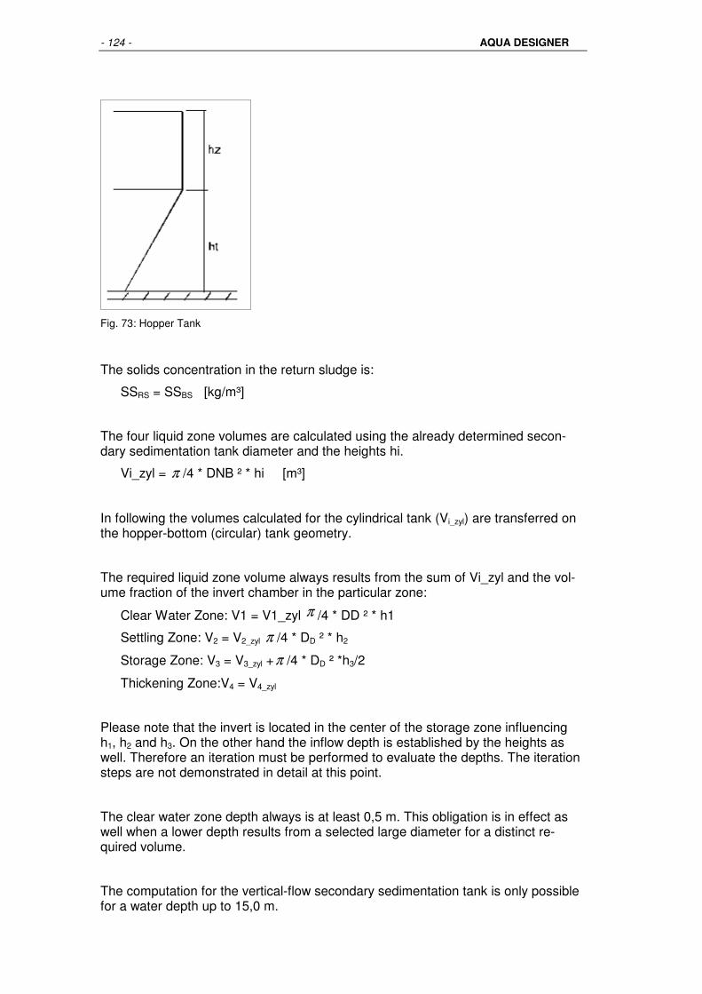
- 124 - AQUA DESIGNER
Fig. 73: Hopper Tank
The solids concentration in the return sludge is:
SSRS = SSBS [kg/m³]
The four liquid zone volumes are calculated using the already determined secon-dary sedimentation tank diameter and the heights hi.
Vi_zyl = π /4 * DNB ² * hi [m³]
In following the volumes calculated for the cylindrical tank (Vi_zyl) are transferred on the hopper-bottom (circular) tank geometry.
The required liquid zone volume always results from the sum of Vi_zyl and the vol-ume fraction of the invert chamber in the particular zone:
Clear Water Zone: V1 = V1_zyl π /4 * DD ² * h1
Settling Zone: V2 = V2_zyl π /4 * DD ² * h2
Storage Zone: V3 = V3_zyl +π /4 * DD ² *h3/2
Thickening Zone:V4 = V4_zyl
Please note that the invert is located in the center of the storage zone influencing h1, h2 and h3. On the other hand the inflow depth is established by the heights as well. Therefore an iteration must be performed to evaluate the depths. The iteration steps are not demonstrated in detail at this point.
The clear water zone depth always is at least 0,5 m. This obligation is in effect as well when a lower depth results from a selected large diameter for a distinct re-quired volume.
The computation for the vertical-flow secondary sedimentation tank is only possible for a water depth up to 15,0 m.
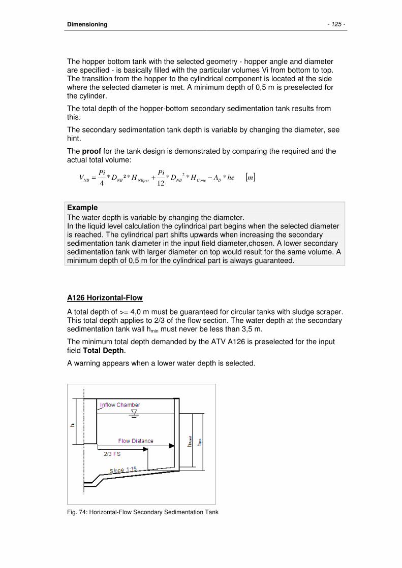
Dimensioning - 125 -
The hopper bottom tank with the selected geometry - hopper angle and diameter are specified - is basically filled with the particular volumes Vi from bottom to top. The transition from the hopper to the cylindrical component is located at the side where the selected diameter is met. A minimum depth of 0,5 m is preselected for the cylinder.
The total depth of the hopper-bottom secondary sedimentation tank results from this.
The secondary sedimentation tank depth is variable by changing the diameter, see hint.
The proof for the tank design is demonstrated by comparing the required and the actual total volume:
[ ]mheAHDPi
HDPi
V DConeNBNBperNBNB ***12
*²*4
2−+=
Example The water depth is variable by changing the diameter. In the liquid level calculation the cylindrical part begins when the selected diameter is reached. The cylindrical part shifts upwards when increasing the secondary sedimentation tank diameter in the input field diameter,chosen. A lower secondary sedimentation tank with larger diameter on top would result for the same volume. A minimum depth of 0,5 m for the cylindrical part is always guaranteed.
A126 Horizontal-Flow
A total depth of >= 4,0 m must be guaranteed for circular tanks with sludge scraper. This total depth applies to 2/3 of the flow section. The water depth at the secondary sedimentation tank wall hmin must never be less than 3,5 m.
The minimum total depth demanded by the ATV A126 is preselected for the input field Total Depth.
A warning appears when a lower water depth is selected.
Fig. 74: Horizontal-Flow Secondary Sedimentation Tank
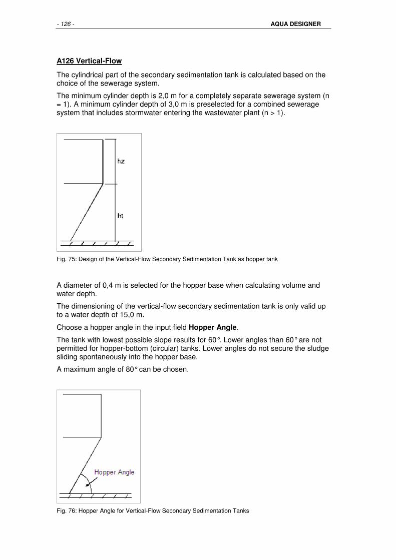
- 126 - AQUA DESIGNER
A126 Vertical-Flow
The cylindrical part of the secondary sedimentation tank is calculated based on the choice of the sewerage system.
The minimum cylinder depth is 2,0 m for a completely separate sewerage system (n = 1). A minimum cylinder depth of 3,0 m is preselected for a combined sewerage system that includes stormwater entering the wastewater plant (n > 1).
Fig. 75: Design of the Vertical-Flow Secondary Sedimentation Tank as hopper tank
A diameter of 0,4 m is selected for the hopper base when calculating volume and water depth.
The dimensioning of the vertical-flow secondary sedimentation tank is only valid up to a water depth of 15,0 m.
Choose a hopper angle in the input field Hopper Angle.
The tank with lowest possible slope results for 60°. Lower angles than 60° are not permitted for hopper-bottom (circular) tanks. Lower angles do not secure the sludge sliding spontaneously into the hopper base.
A maximum angle of 80° can be chosen.
Fig. 76: Hopper Angle for Vertical-Flow Secondary Sedimentation Tanks

Dimensioning - 127 -
A lower angle than 60° can not be chosen as this does not secure the sludge sliding from the tank walls into the hopper. Special constructions should comply with this minimum angle in their angle of intersection.
Partly vertical flown
The limits for the partly vertical flow and the interpolated qSV are
hV/hH <= 0,33 horicontal flown
hV/hH >= 0,50 vertical flown
A relation of 0,33 for example means
hH = 12,0 m
hV = 3,96 m
If the chamber is deaper, hV/hH will increase. The sludge volume load can be higher and the surface decreases.
Fig. 77: Flow conditions in the secondary sedimentaton
Fig. 78: Table11, DWA A 131, Permitted values for partly vertical flown chambers

- 128 - AQUA DESIGNER
Fig. 79: Dimensioning of the partly vertical flown settling tank

Dimensioning - 129 -
Clarified Water Outlet
Two systems are available for the clarified water outlet.
Outlet channels are particularly suitable for small and medium sized horizontal-flow secondary sedimentation tanks.
Immersed pipes are recommended for vertical-flow secondary sedimentation tanks by the ATV.
In AQUA DESIGNER outlet channels may be selected for vertical- and horizontal-flow secondary sedimentation tanks. Immersed pipes are only available for vertical-flow secondary sedimentation tanks.
Immersed Pipes
The outlet pipes located below the water surface are recommended by the ATV for hopper-bottom tanks or vertical-flow secondary sedimentation tanks respec-tively.´The immersed pipes are dimensioned for maximum flow velocity with maxi-mum inflow.
The following upper limits are effective:
Velocity of Flow m/s
Perforations 0,25 Immersed Pipes 1,0 Outlet Pipe 1,0
The immersed pipes are radially arranged and are equally distributed over the sur-face. Their length results from the distance between the inlet and the secondary sedimentation tank wall.
Fig. 80: Immersed Outlet Pipes
The required diameter of the immersed pipes is calculated from the number of pipes and the permitted flow velocity. A standard diameter is suggested from the result.
In the computation form for Immersed Pipes there is the possibility of varying the diameter of the perforations as well as the number of immersed pipes. Selecting a smaller diameter increases the number of perforations.

- 130 - AQUA DESIGNER
Selecting a large number of immersed pipes the required diameter decreases and at the same time the number of perforations per immersed pipe decreases.
Fig. 81: Design of Immersed Pipes
Overflow Weirs
The clarified wastewater leaves the tank via overflow weirs or outlet channels with preceding baffle walls respectively. An outlet channel fixed in 0,5 m distance from the secondary sedimentation tank wall is assumed. The weir loading is calculated from the maximum flow.
Fig. 82: Left: Double-sided overflow weirs; Right: Outlet Channel with preceding Baffle Wall
This is the only available clarified water outlet system for the horizontal-flow circular tank.
For the rectangular chamber overflow weirs may be designed with an overflow to one side or to two sides. The weir load is reduced by half when selecting the over-flow to two sides.
A 126
According to the ATV A126 the weir load is not to exceed 10 m³/(m*h).

Dimensioning - 131 -
A 131
Based on the ATV A131 guideline the weir load should whenever possible stay be-low 10 m³/(m*h) for the single-sided overflow weir and below 6 m³/(m*h) on both sides of the double-sided overflow weir.These values should be further reduced in the case of light sludge with a sludge index above 150 ml/g.
Activated Sludge Tank
Generell
The activated sludge tank was computed in the form Basic Data. The computation steps for evaluating the required volumes were demonstrated. The actual tank ge-ometry is determined in the form Activated Sludge Tank. The proof of the selected design is demonstrated on this basis.
Chamber Construction
Different types of tanks are available for the activated chamber.
The circular or rectangular tank may be selected for the separate construction of activated chamber and sedimentation chamber.
The compact construction system is available either as combined system or circular chamber with flat bottom or as compact system with central hopper-bottom tank.
The compact or separated construction is available for the sedimentation tanks of flat-bottom type or hopper bottom type with the activated chamber as circular or rectangular tank.
Combined systems with central sedimenta-tion with flat bottom
Compact system with central hopper tank
Separate Chamber as circular chamber
Separate chamber as rectangular chamber
Separate chamber as oxidation ditch
Fig. 83: Variation of chamber construction

- 132 - AQUA DESIGNER
Combined Tank System
In the computation form AC (NB intern) in the Main Window NB horizontal tree line a tank geometry for a circular tank with central horizontal-flow secondary sedimen-tation tank is computed. This type of tank is also called a package plant.
Fig. 84: Diagram of a package plant
The required activated sludge tank volume resulting from the computation in the form Basic Data is displayed.
Diameter
The given required diameter is the overall diameter of the package plant. This di-ameter incorporates the inner secondary sedimentation tank wall with its thickness of 30 cm as shown in the form Details. No minimum distance is preselected between the activated sludge tank and the secondary sedimentation tank.
Fig. 85: Form for a package plant design based on the ATV A131
In the input field Diameter, selected the given rounded value may be accepted or another value may be entered.

Dimensioning - 133 -
Water Depth
The indicated depth is equal to the water depth and results from the package plant tank geometry.
The floor level of the activated sludge tank corresponds to the secondary sedimen-tation tank floor level at the rim. You will find this demonstrated in the above draw-ing of a package plant. Because of the hydraulic loss the height of the water level in the activated sludge tank is assumed 10 cm higher than the water level in the sec-ondary sedimentation tank. This value can be changed in the form Details.
Volume
The true activated sludge tank volume is calculated from the water depth and the value that was entered in the input field for Diameter, selected, thus, the dimen-sioning is verified.
True activated sludge tank volume:
VAT = Pi/4* HAT * (DAT2 - (DST + 0,6)2) >= VAT,min
HAT = HNBper + 0,1 (respective chosen level distance)
HAT Water Depth of Activated Sludge Tank [m] DAT Outer free Diameter of the Activated Sludge Tank [m] DST Free Diameter of the Secondary Sed. Tank [m] HSTper Peripheral Water Depth of the Secondary Sed. Tank [m]
A value of 0,3 m is taken into account for the thickness of the secondary sedimenta-tion tank wall.

- 134 - AQUA DESIGNER
Compact Plant
The secondary sedimentation tank is a hopper-bottom tank arranged as centre unit within the activated sludge tank
This tank construction is called a compact plant in following.
Water Depth
The activated sludge tank water depth is selected by the user. The required diame-ter for the activated sludge tank is calculated from the selected water depth and the required volume.
Fig. 86: Compact plant with even base, maximum water depth
A water level difference of 10 cm is taken into account between the activated sludge tank and the secondary sedimentation tank when the tank geometry is determined.
It is only possible to select a water depth smaller or equal to the water depth for a compact plant with even base.
Meaning, the maximum water depth in the activated sludge tank is 10 cm higher than the secondary sedimentation tank water depth.
In Figure 48 ***the base of the secondary sedimentation tank and the activated sludge tank are level. For deep secondary sedimentation tanks it is useful to design the activated sludge tank more flat. In this case a concrete placement funnel is in-troduced into the activated sludge tank base. In following the part of the secondary sedimentation tank above the tank base may be constructed out of metal (alumin-ium or stainless steel) or concrete. An according tank is displayed in the Control Picture.

Dimensioning - 135 -
Fig. 87: Form Compact plant
Diameter
A minimum diameter is calculated for the activated sludge tank using the required volume and the selected water depth.
For compact plants with even base the tank volumes of the activated sludge proc-ess and secondary sedimentation are added and from the result the required acti-vated sludge tank diameter is calculated. For tanks with deeper secondary sedimentation the volume below the tank base is deducted from the secondary sedimentation tank volume.
The difference between the diameters of the activated sludge tank and the secon-dary sedimentation tank should be at least 1,5 m.
In the figur below ***a compact plant with centrally located vertical-flow secondary sedimentation tank is outlined. The hopper ends on one level with the base. The user is free to select a more even activated sludge tank. In this event the hopper base is lower than the base of the activated sludge tank. This is considered when calculating the volume.
Technical Information Circular tanks may be constructed economically as scaled chambers. The tanks offered by the construction companies are levelled in steps. The di-ameters should be selected in 0,5 m steps if this is to be considered in the design. The total depth of the tank is levelled in 0,5 m steps as well whereas the remaining free board may be varied here.
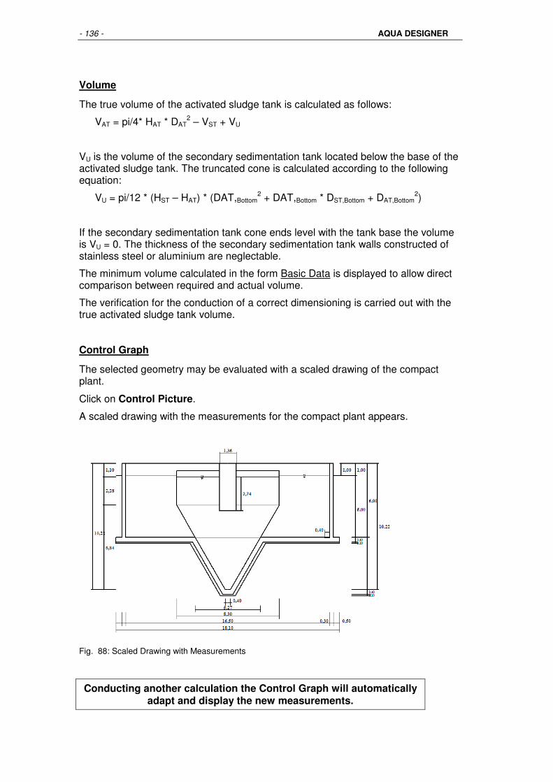
- 136 - AQUA DESIGNER
Volume
The true volume of the activated sludge tank is calculated as follows:
VAT = pi/4* HAT * DAT2 – VST + VU
VU is the volume of the secondary sedimentation tank located below the base of the activated sludge tank. The truncated cone is calculated according to the following equation:
VU = pi/12 * (HST – HAT) * (DAT,Bottom2 + DAT,Bottom * DST,Bottom + DAT,Bottom
2)
If the secondary sedimentation tank cone ends level with the tank base the volume is VU = 0. The thickness of the secondary sedimentation tank walls constructed of stainless steel or aluminium are neglectable.
The minimum volume calculated in the form Basic Data is displayed to allow direct comparison between required and actual volume.
The verification for the conduction of a correct dimensioning is carried out with the true activated sludge tank volume.
Control Graph
The selected geometry may be evaluated with a scaled drawing of the compact plant.
Click on Control Picture.
A scaled drawing with the measurements for the compact plant appears.
Fig. 88: Scaled Drawing with Measurements
Conducting another calculation the Control Graph will automatically adapt and display the new measurements.
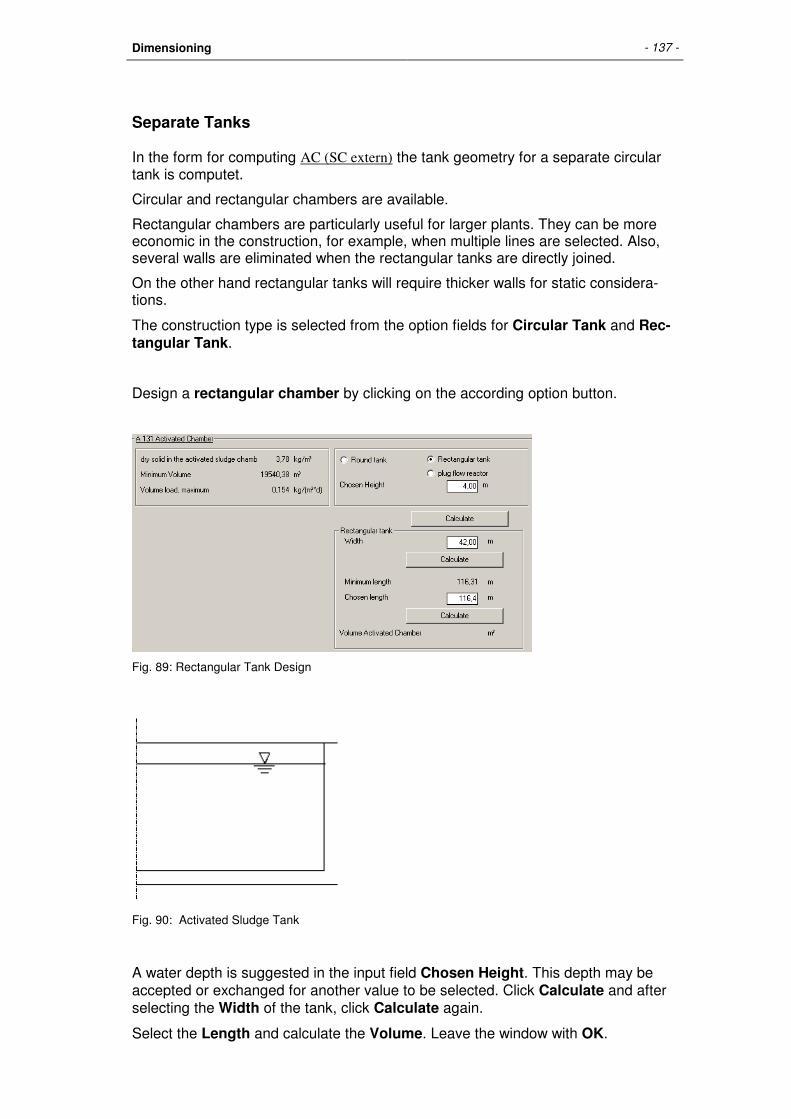
Dimensioning - 137 -
Separate Tanks
In the form for computing AC (SC extern) the tank geometry for a separate circular tank is computet.
Circular and rectangular chambers are available.
Rectangular chambers are particularly useful for larger plants. They can be more economic in the construction, for example, when multiple lines are selected. Also, several walls are eliminated when the rectangular tanks are directly joined.
On the other hand rectangular tanks will require thicker walls for static considera-tions.
The construction type is selected from the option fields for Circular Tank and Rec-tangular Tank.
Design a rectangular chamber by clicking on the according option button.
Fig. 89: Rectangular Tank Design
Fig. 90: Activated Sludge Tank
A water depth is suggested in the input field Chosen Height. This depth may be accepted or exchanged for another value to be selected. Click Calculate and after selecting the Width of the tank, click Calculate again.
Select the Length and calculate the Volume. Leave the window with OK.
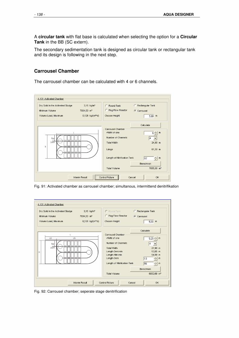
- 138 - AQUA DESIGNER
A circular tank with flat base is calculated when selecting the option for a Circular Tank in the BB (SC extern).
The secondary sedimentation tank is designed as circular tank or rectangular tank and its design is following in the next step.
Carrousel Chamber
The carrousel chamber can be calculated with 4 or 6 channels.
Fig. 91: Activated chamber as carrousel chamber; simultanous, intermittend denitrifikation
Fig. 92: Carrousel chamber; seperate stage denitrification

Dimensioning - 139 -
Volume
Real volume of the activated sludge chamber:
1. Circular chamber
][mD * H * 4
= V 32
ATATAT
π
2. Rectangular chamber
][mB * H * = V 3
ATATAtAT L
Using the real activated sludge tank volume the verification of the dimensioning is conducted.
Technical Information: Deep activated sludge tanks A report of the ATV work group 2.6 on „Aerobe biologische Abwasserre-inigungsverfahren“ (‘Aerobic biological wastewater clarification processes’) points out operational problems with deep activated sludge tanks and fol-lowing conventional secondary sedimentation tanks. More carbon dioxyd is dissolved in the wastewater because of the higher partial pressure in the deep tank. This results in a carbonate balance shift and possibly in a problematic pH value decrease. The pH value decrease may impair nitrification, disintegrate activated sludge flocs and amplify cor-rosion of the concrete. The accumulation of carbon dioxide is enhanced by the low requirement for oxygen as the stripping effect is smaller than in flat tanks. With increased partial pressure in the liquid more nitrogen is dissolved in the wastewater. This dissolved nitrogen will be released with reduced par-tial pressure. The developing gas bubbles may lead to flotation and, thus, sludge loss.
Verification
The activated sludge tank geometry may be influenced by the user through the in-put fields for water depth or diameter. Therefore a verification is required for the different parameters of the ATV guidelines A126 und A131. The verification of the dimensioning can be reviewed in the print-out of the technical wastewater plant computation.
A131
The dimensioning based on the A131 is verified through the sludge age. Initially the real sludge load is evaluated:

- 140 - AQUA DESIGNER
d*kg
kg
SS * V
B = B
ATAT
BOD5d,
SS
The real sludge age tTS is calculated according to the following equation:
d*kg
kg
t* ) WS+ (WS
1 = B
SSPBOD5
SS
Note that the biological excess sludge production is dependent on the sludge age as well. A quadratic equation results that is to be solved for tTS.
A126
The verification for the A126 is simplified and results from the sludge load:
d*kg
kg
TS * V
B = B
ATAT
BODd,
SS5
In contrast to the A131 the sludge age is not considered in the dimensioning of the activated sludge process.

Dimensioning - 141 -
Aeration
Generell
The oxygen demand with the resulting air consumption is computed and the accord-ing machinery is selected taking into account the tank geometry.
Preselections have been made depending on the selected clarification processes. For example a mixing device is automatically suggested when denitrification is se-lected.
The required blowers and mixing devices are available from data banks.
For designing the aeration a detailed form membrane aeration is available. It offers a particularly flexible and individual design of the aerator elements and distribution.
Oxygen Demand
ATV-A131, Specific Oxygen Demand
The BOD5- and N-load as well as the selected clarification processes are the foun-dation for the computation of the oxygen demand.
The specific oxygen demand (OVC and OVN) results mainly from the degradation of organic carbon compounds and nitrogen compounds by micro-organism.
OVC names the specific oxygen demand for the degradation of carbon compounds and results from the following equation:
ATV-A131, 2000
For CCOD,ZB/CBOD,ZB ≤ 2:
++=
5
2,
*17,0*1
**15,056,0
kgBOD
kgO
Ft
FtOU
TSS
TSSCd
F = 1,072(T-15) Temperature Faktor TSS Sludge Age [d]
For CCOD,ZB/CBOD,ZB >2 the specific oxygen demand has to be calculated based on the COD.
Information: The higher the sludge age the better the degradation of the organic matter and thus, the degree of sludge mineralisation. Oxygen is required for the degradation steps. Therefore the specific oxygen demand for carbon com-pound degradation OVC increases with increasing sludge age. The velocity of chemical and biological reactions increases with an in-crease of the temperature. Hence the oxygen demand rises with the tem-perature as well.

- 142 - AQUA DESIGNER
The upper value limit for the OVC is 1,6 kgO2/kgBOD5. according to the ATV A131 guideline.
T °C Sludge Age in Days 15 25 10 1,32 1,55 12 1,38 1,60 15 1,46 1,60 18 1,54 1,60 20 1,60 1,60
Excerpt from Table 10, A131; Specific Oxygen Demand OVC in kgO2/kgBOD5
The specific oxygen demand for the degradation of nitrogen compounds OVN is dependent on the selection of nitrification and/or denitrification for clarifying proc-esses. In the nitrification process oxygen is required for oxidation of ammonia to nitrite and nitrate as demonstrated in the chemical equations in the chapter on the foundations.
The nitrate is reduced to elementary nitrogen and in a small amount to N2O in the denitrification process. The nitrate nitrogen is used for the anoxic respiration. The denitrification reduces the required oxygen demand for nitrogen compound degra-dation.
On the basis of the above described processes OVN results in:
+−=
d
kgOSSSQOU ANNOZBNODNO
dNd
2
1000*3,4*
,3,3,3
,
−=
d
kgOSQOU DNO
dDd
2
1000*9,2*
,3
,
NO3-Ne Nitrate-N concentration in outlet (outflow) [mg/l] NO3-ND Denitrified nitrate concentration [mg/l] BOD5 BOD5 concentration in inlet (inflow) [mg/l]
ATV-A131, Oxygen Charge
Shock loads must be considered for evaluating the oxygen charge. Therefore shock factors (fC, fN) are introduced for nitrogen and carbon compounds. These are pre-sented in the following table referring to the range of application in the AQUA DESIGNER and based on the ATV A131.
Sludge Age in Days T in °C 15 25
fC 1,15 1,10 fN for <= 20.000 EW 2,00 1,50 fN for > 100.000 EW 1,50 -
Table 10, Shock factors according to ATV A131
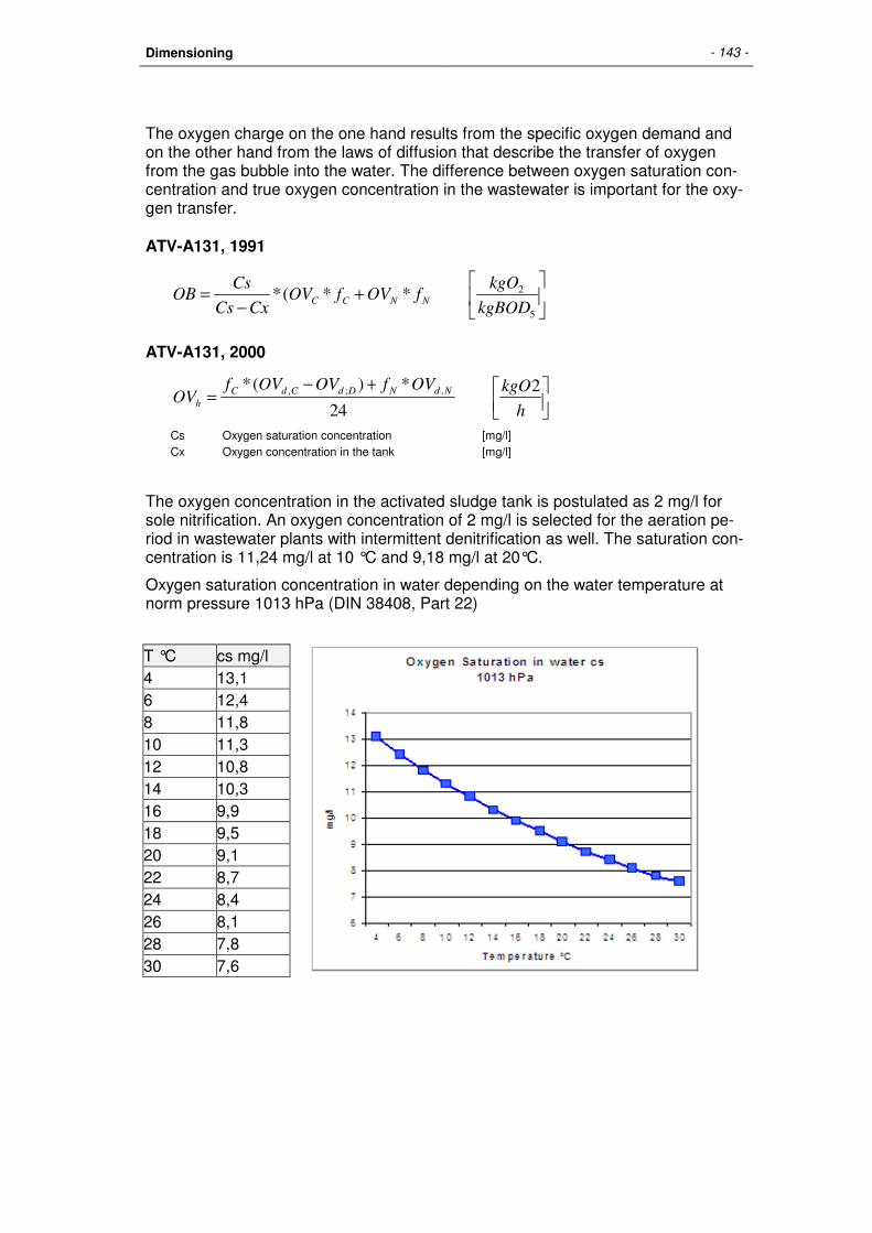
Dimensioning - 143 -
The oxygen charge on the one hand results from the specific oxygen demand and on the other hand from the laws of diffusion that describe the transfer of oxygen from the gas bubble into the water. The difference between oxygen saturation con-centration and true oxygen concentration in the wastewater is important for the oxy-gen transfer.
ATV-A131, 1991
+
−=
5
2**(*kgBOD
kgOfOVfOV
CxCs
CsOB NNCC
ATV-A131, 2000
+−=
h
kgOOVfOVOVfOV NdNDdCdC
h
2
24
*)(* ,;,
Cs Oxygen saturation concentration [mg/l] Cx Oxygen concentration in the tank [mg/l]
The oxygen concentration in the activated sludge tank is postulated as 2 mg/l for sole nitrification. An oxygen concentration of 2 mg/l is selected for the aeration pe-riod in wastewater plants with intermittent denitrification as well. The saturation con-centration is 11,24 mg/l at 10 °C and 9,18 mg/l at 20°C.
Oxygen saturation concentration in water depending on the water temperature at norm pressure 1013 hPa (DIN 38408, Part 22)
T °C cs mg/l 4 13,1 6 12,4 8 11,8 10 11,3 12 10,8 14 10,3 16 9,9 18 9,5 20 9,1 22 8,7 24 8,4 26 8,1 28 7,8 30 7,6
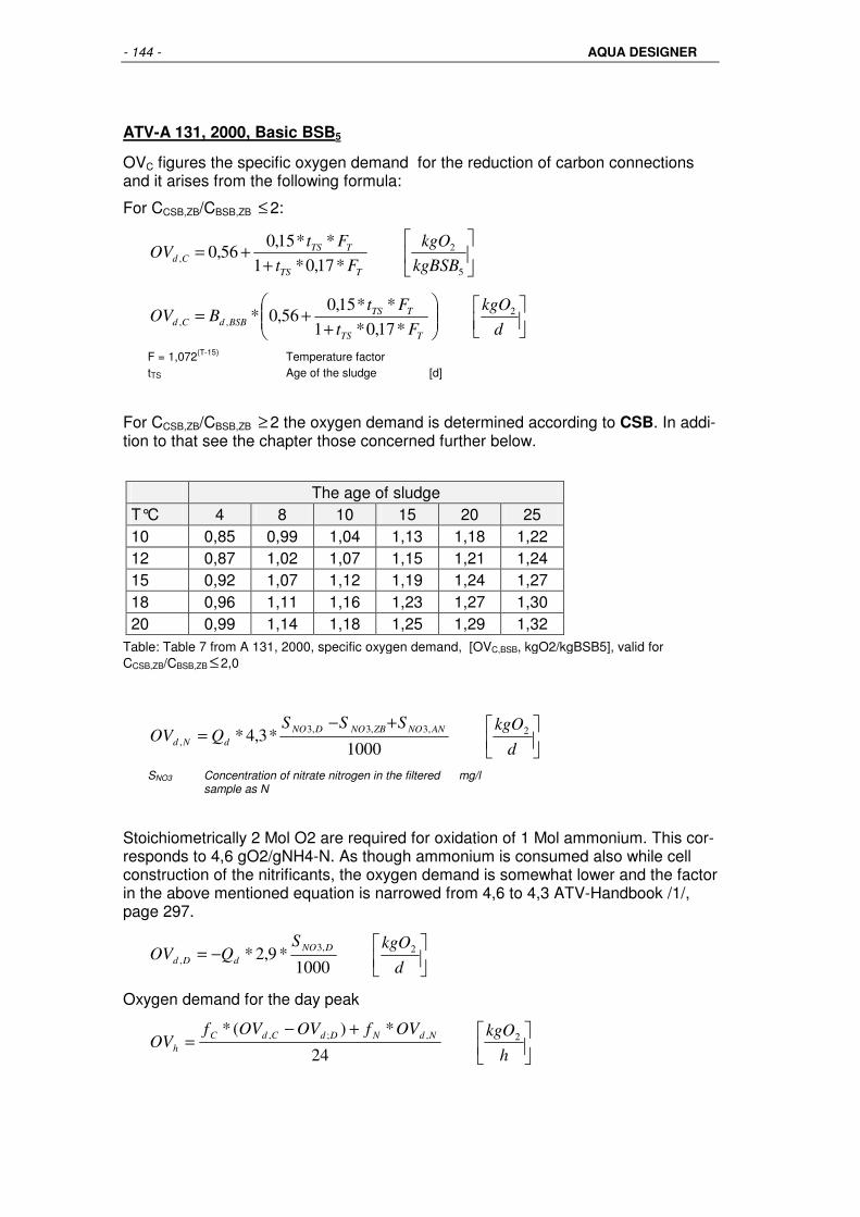
- 144 - AQUA DESIGNER
ATV-A 131, 2000, Basic BSB5
OVC figures the specific oxygen demand for the reduction of carbon connections and it arises from the following formula:
For CCSB,ZB/CBSB,ZB ≤ 2:
++=
5
2,
*17,0*1
**15,056,0
kgBSB
kgO
Ft
FtOV
TTS
TTSCd
++=
d
kgO
Ft
FtBOV
TTS
TTSBSBdCd
2,,
*17,0*1
**15,056,0*
F = 1,072(T-15) Temperature factor tTS Age of the sludge [d]
For CCSB,ZB/CBSB,ZB ≥ 2 the oxygen demand is determined according to CSB. In addi-tion to that see the chapter those concerned further below.
The age of sludge T°C 4 8 10 15 20 25 10 0,85 0,99 1,04 1,13 1,18 1,22 12 0,87 1,02 1,07 1,15 1,21 1,24 15 0,92 1,07 1,12 1,19 1,24 1,27 18 0,96 1,11 1,16 1,23 1,27 1,30 20 0,99 1,14 1,18 1,25 1,29 1,32
Table: Table 7 from A 131, 2000, specific oxygen demand, [OVC,BSB, kgO2/kgBSB5], valid for CCSB,ZB/CBSB,ZB ≤ 2,0
+−=
d
kgOSSSQOV ANNOZBNODNO
dNd2,3,3,3
,1000
*3,4*
SNO3 Concentration of nitrate nitrogen in the filtered sample as N
mg/l
Stoichiometrically 2 Mol O2 are required for oxidation of 1 Mol ammonium. This cor-responds to 4,6 gO2/gNH4-N. As though ammonium is consumed also while cell construction of the nitrificants, the oxygen demand is somewhat lower and the factor in the above mentioned equation is narrowed from 4,6 to 4,3 ATV-Handbook /1/, page 297.
−=
d
kgOSQOV DNO
dDd2,3
,1000
*9,2*
Oxygen demand for the day peak
+−=
h
kgOOVfOVOVfOV NdNDdCdC
h2,;,
24
*)(*

Dimensioning - 145 -
Age of sludge in days 4 6 8 10 15 25 fC 1,3 1,2
5 1,2 1,2 1,1
5 1,10
fN for <= 20.000 EW - - - 2,5 2,00
1,50
fN for > 100.000 EW - - 2,0 1,8 1,50
-
Table: Impact factors for the oxygen demand (to cover, 2-h-peak opposite to 24-h-means, if no meas-urements are available.); Table 8 from A 131, 2000
The impact factor fN reflects the interrelation between the ammonium freight in the peak hour and the average freight.
At fC it is not the case, for the hydrolysis of the sediments affect in a compensative way.
Required oxygen supply for continuously aerated basins:
−=
h
kgOOV
CxCs
CsOCerf h
2*.α
Required oxygen supply for intermittent aeration:
−−=
h
kgO
VVOV
CxCs
CsOCerf
BBD
h2
/1
1**.α
Cx Content of oxygen in an aerated part during aeration
period mg/l
Cs Concentration of oxygen saturation mg/l
Cx= 2 mg/l
Whitlow basins with simultaneous denitrification and surface aerators:
Cx = 0,5 mg/l
Low Loads
If the load of the plant is less than 30% in comparison with the average calculated capacity, it is necessary to determine the supply of oxygen fN = 1 and fC = 1 for the real load. This value serves for the better gradation of the fans, resp. aeration units. You can easily determine the gradation through the consideration of loading condi-tions under Extras > Calculation of loading conditions.

- 146 - AQUA DESIGNER
Adaption of Saturation Concentration
Conversion based on working pressure
The concentration of oxygen saturation is dependent on the working pressure. While the pressure increases, the solubility of oxygen also intensifies. It means for the determination of the oxygen demand at compressed aeration, that the concen-tration of oxygen saturation is higher at the blow-in point than at the water surface. The dependence of the solubility upon the depth level of the blow-in point is taken into account through average pressure. The average pressure corresponds to the hydrostatic pressure at the half depth of the blow-in point.
For the conversion of the solubility of oxygen from environment pressure into the pressure at the half blow-in point Wagner /28/ indicates a correction factor:
][7,20
1*,l
mgdecsmcs
+=
de Depth of the blow-in point m 20,7/2 =10,33 Pressure at 1013,25hPa mWS
In the A131 this correction factor was not indicated. In comments to A131 from Kay-ser /45/ this adjustment was however also applied. Therefore in practice it should be taken into account.
Higher reaction temperature
If you select higher reaction temperature, resp. dimensioning temperature higher than 10°C, the loading conditions for maximum C and N-pollution are also calcu-lated for the selected temperature and taken into account while choosing the maxi-mum of the loading conditions.
According to Lutz Härtel /1/ the concentration of oxygen saturation can be calcu-lated dependent on the temperature.
]³
[)93,45(
34,2234 theor.Cs, 2
31403,1 m
gO
T +=
Pöpel additionally indicates a correction factor for the depth of the blow-in point.
]³
[hE) * 0,1 (1 * theor.cs, HCs, 2
m
gO+=
ATV-A 131, 2000, Basic CSB
OVC figures the specific oxygen demand for the reduction of the carbon connec-tions and based on CSB results in

Dimensioning - 147 -
Oxygen demand:
][,,l
mgXSCOV ÜSANinertZBCSBC −−=
][1000
)(*2,
,d
kgOXSCQdOV ÜSANinertZB
Cd
−−=
][1000*
)(*2
,
,
kgCSB
kgO
B
XSCQdOV
CSBd
ÜSANinertZB
C
−−=
The further calculations are represented as in the preceding chapter for BSB5.
Loading conditions
ATV-A131
To determine the maximum oxygen load, various loading conditions are calculated : three different temperatures are taken into account.
Loading condition winter The temperature, which is also accepted while calculating the volumes of the vitalizing sludge basin under loading conditions winter, is also accepted as the lowest tempera-ture. It is the lowest 2 weeks average temperature in win-ter. Here in Germany the temperature of is usually accepted.
Dimensioning temperature
The average loading condition is the oxygen demand at the measured temperature. The recommended measured temperature is 12°C in Germany.
Highest temperature 20°C is usually accepted as the highest temperature. Due to lower solubility of oxygen in water at higher tempera-tures, this temperature is determined to be the most unfa-vourable loading condition for the aeration.
Different loads are computed to evaluate the maximum oxygen charge:
Nitrification/Denitrification
Temperature 10 °C
• Maximum C-load, medium N-load
• Medium C-load, maximum N-load
Temperature 20 °C
• Maximum C-load, medium N-load
• Medium C-load, Maximum N-load

- 148 - AQUA DESIGNER
Nitrification
Temperature 10 °C
• Maximum C-load, medium N-load
• Medium C-load, maximum N-load
Medium N-load always refers to a shock factor of fN equal to 1. This applies ana-logue to the medium C-load.
Altogether six events of loads are reviewed when selecting nitrifica-tion/denitrification. Without denitrification only the two loads for 10°C result. The oxygen charge results as maximum from the examined load cases. Note that different aeration periods apply for nitrification and denitrification.
Technical Information The metabolism for degradation of organic compounds and nitrification is dependent on the oxygen concentration in the activated sludge tank. The higher the oxygen concentration in the activated sludge tank the faster the biochemical reactions. The relation corresponds to 1st class chemical reac-tions.
)(* CCskLadt
dc−=
Experiments show an economic operation of the aeration when maintaining an oxygen concentration of about 2 mg/l. For maintaining higher oxygen concentrations in the activated sludge tank the additional aeration energy consumption in the activated sludge tank outweighs the increase in metabolism. The nitrification reaction velocity reduces considerably for oxygen concen-trations below about 0,5 mg/l.
The oxygen charge evaluated according to the described algorithm is valid for oxy-gen transfer in clear water. Consumptive processes occur in the wastewater. There-fore more oxygen must be transferred into the wastewater in order to maintain the selected oxygen concentration.
The oxygen supply factor α is introduced for the conversion of the oxygen demand of clear water to wastewater. The oxygen supply factor is dependent on the se-lected aeration system and on the water depth. Pöpel gives oxygen supply factors for different aeration systems /15/.
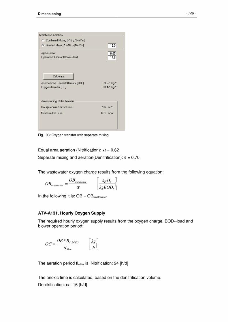
Dimensioning - 149 -
Fig. 93: Oxygen transfer with separate mixing
Equal area aeration (Nitrification): α = 0,62
Separate mixing and aeration(Denitrification):α = 0,70
The wastewater oxygen charge results from the following equation:
=
5
2
kgBOD
kgOOBOB purewater
wastewaterα
In the following it is: OB = OBwastewater.
ATV-A131, Hourly Oxygen Supply
The required hourly oxygen supply results from the oxygen charge, BOD5-load and blower operation period:
=
h
kg
tL
BOBOC BODd
dim
5,*
The aeration period tLdim is: Nitrification: 24 [h/d]
The anoxic time is calculated, based on the denitrification volume.
Denitrification: ca. 16 [h/d]

- 150 - AQUA DESIGNER
ATV-A126
The tubular diffuser fine bubble aeration with combined and separate mixing is the available aeration system.
In contrast to the A131 a value is preselected for the oxygen charge:
OB = 3,0 [kg/kg]
The hourly oxygen supply results as follows:
=
h
kg
tL
BOBOC BODd
dim
5,*
Aeration Period tLdim:
Nitrification: 24 [h/d]
Denitrification: 16 [h/d]
This value generally covers the micro-organism oxygen consumption for nitrogen and carbon oxidation. Is the ratio
TKN : BOD5 < 1 : 3,5 in the influent
above the limit, it is recommended to demonstrate the required oxygen demand for nitrogen oxidation separately.
Membrane Aeration
Most commonly the air is introduced with tubular diffusers in pneumatic aeration. For this type of aeration suitable values are preselected in the AQUA DESIGNER forms. Product specific data may be entered into the according input fields for dif-ferent types of aerators, for example ceramic aerators.
Air Consumption
In the form Aeration an oxygen transfer capacity of 8 g/(m³*m) is preselected for the combined mixing and aeration. Here the ATV recommends
−=
m*m³
g 1082fO
The separate mixing and aeration is recommended for wastewater plants serving a population equivalent of more than 600. This also applies when denitrification is not required. Otherwise sludge deposition in critical tank areas is to be expected.
The oxygen transfer is preselected as 12 g/(m³*m). Here the ATV guideline recom-mends
−=
m*m³
g 15122fO

Dimensioning - 151 -
The required hourly air volume results from the evaluated hourly oxygen supply and the immersion depth.
h
m
h * fO
1000 * OC = Q
3
E2
L
QL req. hourly air volume [m³/h] fO2 Oxygen transfer factor [g/(m³*m)] hE Immersion depth [m] OC Oxygen supply [kg/h]
Technical Information: The immersion depth is set 30 cm above the tank base being 30 cm less than the activated sludge tank water depth. This is an effect of the aeration system construction. The aeration plugs or discs are fixed to aeration screens set up on the activated sludge tank base. In the form for Details (Menu Options → Details) you can access the im-mersion depth and change the distance between injection depth and water depth.
Fig. 94:Immersion depth
Blower
The number of blowers is entered in the window for selecting the blowers. The re-quired blower air volume results from the calculation of the required air volume and the number of blowers.
The blowers are selected from the data bank. See the chapter on data banks for details on data bank function and operation.

- 152 - AQUA DESIGNER
Fig. 2: Selecting the blower
A stand by blower is not considered in this calculation. Thus, when selecting three blowers these three blowers are used in the further set up of the aeration operation.
When selecting multiple parallel lines or multiple activated chambers, respectively, two blowers are suggested for each line by the program appearing in the field Num-ber of Blowers. You may enter any other number of blowers. The total capacity of the blowers will be equally distributed on the lines.
Aeration Devices
Clicking on Membrane Aeration leads you to the aeration system design after hav-ing completed the previous calculations in the aeration form.
The Membrane Aeration form consists of three parts.
The left part allows the design of the aeration unit by entering data and selecting options.
The right upper part displays the complete unit arrangement for one chamber.
The right lower part displays a magnified lattice. In this window characteristic data of the complete system and of one lattice are presented.
Fig. 95: Characteristic data for one lattice
All values displayed in the Membrane Aeration form refer to one chamber only.

Dimensioning - 153 -
Design of Lattices
In the window for the design of the lattices the aeration lattices are designed and the distribution of aeration and circulation in one activated chamber is determined.
The input field Number of Lattices determines the number of lattices distributed in each chamber. AQUA DESIGNER calculates the required number of tubes or discs per lattice based on the required air volume and the number of lattices. The air vol-ume flow results from the blower capacity.
You may select tubular diffusers or aerator discs by clicking on the according option in the program.
The field Mixer 1 Group enables you to distribute the mixers in the chamber. One mixer per group is preselected by the program. This determines the uniform distri-bution of the mixers around the circumference (for circular chambers) or over the length (for rectangular chambers).
Fig. 96: Selection of mixers per group, one mixer per group in the left example and two mixers per group in the right example
Enter the value 2 into the input field Mixer 1 Group for placing two mixers close together or two mixers per group. Two segments are set up in the chamber when selecting a total of four mixers for one chamber and two mixers per group.
The type of lattice is determined by entering the Number of Header Pipes in the window for Design of Header Pipes. This decides over the connection of the aera-tors to the central pipe or to distributing header pipes.
Fig. 97: Aeration lattice without header pipes, Schlauchbelüfter = tubular aerators, Zentralrohr = center pipe

- 154 - AQUA DESIGNER
Fig. 98: Aeration lattice with header pipes
Schlauchbelüfter = tubular aerators Zentralrohr = center pipe Querverteiler = header pipe
When selecting more than one header pipe the equal or graded distribution of membrane aerators is available. For example for the circular chamber it may be useful to reduce the number of tubes or discs towards the centre as the water vol-ume is larger in the outer parts and more air volume is required here.
When selecting aerator discs corresponding header pipes must selected as it is not possible to connect discs directly to the central pipe.
In the input field for Steps (Grading) the graded distribution of discs or tubes is selected and modified.. This is particularly useful for lattices with disc aerators. A large number of header pipes is usually selected for disc aerators. By entering 3 for the grading it is possible to reduce the number of discs on each header pipe after every third header pipe.
You have 3 options to choose the kind of aera-tor:
• Tubular aeraters
• Aeration discs
• Aerator panel
In the window for tubular diffuser and disc aera-tor the geometry of the aerators is determined and the load per aeration unit is entered. When selecting tubular diffusers the according window is open. Here the length for one aeration unit and the load per meter of aerator is entered.
Fig. 99: Window for determining lattices

Dimensioning - 155 -
The required aeration plug length results from the recommended aerator load that is the introduced air volume per aerator length.
][mB
QLL
Aerator
Aerator =
LAerattor effective aerator length [m] QL hourly air volume current [m³/h] BAerator Aerator load [m³/(m*h)]
The aerator load is preselected in the input field Load of Aerators, max. The user may select a higher or lower aerator capacity.
Economic operational results are achieved with plug capacities of about
h * m
m³ 7,5 = BAerator
Technical Hints: With an increase of the aerator load the pressure drop increases. This has a negative impact on the operation costs. Therefore operation and invest-ment costs are to be weighed in the layout. The aerators are produced in different lengths. One segment usually con-sists of two plugs of 0,75 m or 1,0 m length. From that a construction group results consisting of two plugs with a total length of 1,5 m or 2,0 m. These plugs are arranged at distributing pipes as a screen.
When disc aerators were selected the according window is open. Enter the diame-ter of the disc aerators into the input field for Diameter of disc aerators. The value depends on the selected manufacturer. The suggested value is based on the most common designs.
Note that the disc aerator design is not based on its surface area. The aerator load is given per aerator unit or per disc as commonly practised.
nTeller
TellerB
QL=
Ndiscs Number of discs QL Hourly air volume current [m³/h] BDisc Disc aerator load [m³/(Disc*h)]
h * disc
m³ 8,0 = BTeller
For aerator panels the surface loading defines the number of aerators. The size and geometrie will be entered here.

- 156 - AQUA DESIGNER
Fig. 100: Aerator panel in a nitrification chamber
*
n
panelpanel
panelAB
QL=
ndiscs Number of discs QL Hourly air volume [m³/h] Bpanel Surface loading of panels [m³/(m²*h)] Apanel Surface of the panels m²
h * disc
m³ 25,0 = Bpanel
Equipment
Further aeration design is available through the Equipment option. Here the dis-tance of the lattices from the tank wall and the distance between plugs and discs may be varied.
Fig. 3: Window for Construction through according button

Dimensioning - 157 -
For example a more uniform distribution of discs on the tank base may be obtained through this option. For narrow circular tanks, for example small compact tanks, it may be useful to reduce the distance between the lattices and the tank wall.
Output
Click on Output to update the graphical display after changing data in the windows for Construction or Determining lattices.
Mixing Devices
Combined mixing and aeration defines the introduction of the required oxygen into the activated sludge tank and at the same time the maintenance of the activated sludge suspension by means of aeration. An additional mixing device is unneces-sary. Mixing devices are installed in the case of separate mixing processes.
Combined Mixing and Aeration
In pure nitrification operation the circulation may take place through the aeration only. In this case extended periods without aeration must be avoided in the reactor. In the past it has been demonstrated that population equivalents above 600 require mixing devices to avoid deposition of material in the rim areas.
Separate Mixing
The circulation is maintained through mixing devices selected from the data bank. Enter the number of mixers into the input field Number of Mixers. One mixer for each chamber or line is preselected by the program.
For example one mixing device per activated chamber is present when three mixing devices are suggested in the input field for the Number of mixing devices and when three activated chambers were selected.
Fig. 101: Selecting the mixing device
See the chapter on data banks for details on data bank function and operation.
The ATV A126 suggests an energy input of 3 - 8 W/m³ by the mixing device. Lower values are sufficient for favourable tank types. The selection of a lower energy input should be co-ordinated with the mixing device manufacturer. Suggestions for ar-rangement and design are readily carried out by the supplier.

- 158 - AQUA DESIGNER
Technical Information It is recommended to use slow circulating mixers for mixing the activated sludge if the tank measurements allow. These mixers have large propeller diameters and are more economic than fast rotating mixers. The energy consumption of the mixers strongly influence the energy costs as the mix-ing devices are generally operated around the clock. In the Aeration form the mixer data bank lists several slow rotating mixers of established manufacturers/ companies. In the evaluation of the operation costs the major part of the energy costs are the costs for aeration. Therefore the aeration system should be care-fully designed. A uniform distribution of the aeration over the tank base surface improves the economy of the aerators. A fine tuning of the blowers improves their efficiency.
Surface Aeration
Membrane aeration or surface aeration may be selected for oxygenation. AQUA DESIGNER offers two different sets of machinery for the surface aeration that is the surface mechanical aerator with vertical or horicontal axis. For the vertical axis aera-tor the use in mixing chambers or circulation systems is defined.
Required Oxygenation
The required oxygenation is evaluated from the ratio of oxygen transfer capacity to BOD5-load related to the volume. This value allows the calculation of the required energy density and thus, the selection of the aeration machinery.
Required oxygenation:
=
hm
kgO
V
OBOCA
AT
serSchmutzwas
*³
2
The required values are evaluated for three different cases based on the recom-mendations of Wagner /28/,. The desired case is selected with the menu bar op-tions.
Evaluating the required oxygenation in different operating states:

Dimensioning - 159 -
Rotor in the tank with circulating flow:
Oxygen transfer capacity:
+=
hm
gOLDOCA
BB *³*40,175,11 2
Oxygen transfer efficiency:
−=
kWh
kgOLDON 2*0058,097,110
Surface mechanical aerator with vertical axis in the tank with circulating flow:
Oxygen transfer capacity:
+−=
hm
gOLDOCA
BB *³*58,205,2 2
Oxygen transfer efficiency(statistically unproved):
−=
kWh
kgOLDON 2*0121,036,210
Surface mechanical aerator with vertical axis in the mixing chamber:
Oxygen transfer capacity:
+−=
hm
gOLDOCA
BB *³*96,173,10 2
Oxygen transfer efficiency:
+=
kWh
kgOLDON 2*0055,041,110
The above cases were statistically evaluated and thus, represent average values for different methods of aeration under the different given conditions.
Selected Oxygenation
After evaluating the required oxygenation there is the possibility to enter a value of your own choice, for example on the base of operational experience. The aeration machinery is calculated based on the selected oxygenation. Enter the desired num-ber of aeration sets. In following the required capacity for one set is given. For se-lecting a defined aerator with variable motor power the capacity of the selected aerator may be entered into the field for Selected capacity per aerator.

- 160 - AQUA DESIGNER
Leave Form
Leave the form with OK. Changes in the input are accepted and saved by the pro-gram without using the Output button. In this case the graphical display, however, will not show the latest changes.
Leaving the form with Cancel the latest changes are not saved.
Return Sludge Transport
The recirculation ratio was determined in the form Basic Data. The secondary sedi-mentation is dimensioned with the previously selected recirculation ratio.
In the form Return Sludge the machinery for the return sludge transport is selected. The capacity of the selected units is not considered in the dimensioning of the sec-ondary sedimentation tank. It is assumed that the selected recirculation ratio is maintained by automatic control and regulatory mechanisms.
In the form Return Sludge Transport three different transport units are offered. The recirculation ratio selected in the form Basic Data is displayed. Decide by selecting an option field.
The chapter on Loads also covers control processes and limits for the recirculation ratio.
Recirculation Rate QRS
The required transport volume is displayed in the window for dimensioning the transport unit. The transport volume results from the recirculation ratio that was en-tered into the form for Basic Data.
The displayed flow rate is:
QRS = RV * Qm [m³/h]
The ATV A131 guideline, part 4.2.3., offers recommendations for the design of the return sludge recirculation unit.
Horizontal flow secondary sedimentation tank: QRS <= 1,5 * Qt
Vertical flow secondary sedimentation tank: QRS <= 2,0 * Qt
The ATV work sheet ‘A131-Secondary Sedimentation Tanks’ adds that for com-bined wastewater inflow the transport unit should be designed for a maximum flow rate of 1,0 * Qm. For vertical flow secondary sedimentation tanks the maximum re-circulation ratio of QRS = 1,0 * Qm can be selected in the design. The pumps should be designed for 1,5 * Qm.
This should be considered when selecting a transport unit from the data bank. Thus, compared to the displayed flow rate a larger unit should be selected.

Dimensioning - 161 -
Membrane System
Membrane Activated Sludge SystemBasic of the Calculation is a Worksheed of the ATV-DVWK-Fachausschusses KA-7 "Membranbelebungsverfahren", opend in Kor-respondenz Abwasser 10/2000.
Activated Chamber
General basic of the Calculation is the Guideline ATV-DVWK-A131 (2000). This means also the Excess-Sludge-Production and Oxygen demand for MLSS-Concentrations less than 5 kg/m³.
Oxygen demand and oxygen input
Oxygen input for Carbon-Degradation:
][
*1
*
**1
5
2
/
0/
0/0
kgBSB
kgO
tmY
Y
tYmOV
TSS
SX
X
TSXC
+
+=
TS kg/m³ 5 10 15 20 α -Wert 0,73 0,42 0,22 0,15
Excess Sludge Production
( )5/
/
55
5**1
)*1(**1***
kgBSB
kgTS
tYm
fcYfc
BSB
TSoa
BSB
PcÜS
TSSXS
PFällSXPFällFällBSB
+
−+−+=
Coeffizient Value Description Dimension YX/S 0,6 Yield, for BOD5
5kgBSB
kgX
YX/O 1,2 Yield, for Oxygen
2kgO
kgX
mS 0,133 obtaining coefficient, for BOD5
dkgX
kgBSB
*
5
mO 0,24 obtaining coefficient, for Oxygen
dkgX
kgO
*
2
a 0,5 Inert parts of Tso (Dry Solids, inflow) - cFäll 9 (Fe)
7 (Al) for chemical Phosphate-El.
FällkgP
kgTS
fP 0,025 Phosphate in the biomass and in inert parts of inflow dry solids
-

- 162 - AQUA DESIGNER
Membrane Dimensioning
Specific Permeate Flow:
]*²
[*1
hm
l
T
VP
AMAM
PPvP
∆
∆==
Maximum Operation Flows 25 - 30 l/(m²*h) for 10°C.
Transmembrane Pressure Difference
][2
barPPPKpF
PTM −+
=∆
Hydraulical Permeability
]**²
[barhm
l
PTS
VPLP
∆=
QP 1/h PP bar vP l/(m²*h) QF 1/h PF bar QK 1/h PK bar AM m² wÜ m/s
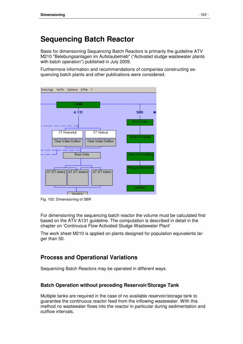
Dimensioning - 163 -
Sequencing Batch Reactor
Basis for dimensioning Sequencing Batch Reactors is primarily the guideline ATV M210 "Belebungsanlagen im Aufstaubetrieb" (“Activated sludge wastewater plants with batch operation”) published in July 2009.
Furthermore information and recommendations of companies constructing se-quencing batch plants and other publications were considered.
Fig. 102: Dimensioning of SBR
For dimensioning the sequencing batch reactor the volume must be calculated first based on the ATV A131 guideline. The computation is described in detail in the chapter on ‘Continuous Flow Activated Sludge Wastewater Plant’
The work sheet M210 is applied on plants designed for population equivalents lar-ger than 50.
Process and Operational Variations
Sequencing Batch Reactors may be operated in different ways.
Batch Operation without preceding Reservoir/Storage Tank
Multiple tanks are required in the case of no available reservoir/storage tank to guarantee the continuous reactor feed from the inflowing wastewater. With this method no wastewater flows into the reactor in particular during sedimentation and outflow intervals.

- 164 - AQUA DESIGNER
Batch Operation with preceding Reservoir
A preceding reservoir/storage tank offers the convenient opportunity to design the operation in one cycle. High organic particle concentrations are achieved in the start interval through short-time input,thus, improving sludge properties and enhancing respiration.
Improved results from denitrification are achieved when the wastewater progresses in multible batches.
Variation of Method
Wastewater plants may be designed on the basis of constant inflow volume or con-stant cycle period in addition to the method of input. The design based on constant cycle period has been widely accepted in practice as it offers transparency during operation. Particularly with multible tanks the current status of each tank is always known.
Cycle Period
The hydraulic detention period may be specified as the ratio of the hydraulic deten-tion period in continuous flow wastewater plants. (Equation 4, work sheet M210)
tZ = ΘH * fA [h] tZ Cycle period h ΘH Hydraulic detention period in the continuous flow activated sludge
reactor h
fA Exchange ratio
The volume exchange ratio is the ratio of the removed volume during one cycle to the reactor volume with maximum fluid level.
VR
VfA
∆=
The wastewater inflow per day must be treated in the present reactors determining the required single reactor volume. The cycle phases are entered into the form Re-
actor Volume.
Period
The cycle period for storm weather and dry weather conditions are entered. The required hydraulic volume depends on the inflow. The required hydraulic volume is reduced when a shorter cycle period is accepted for combined wastewater inflow. The result window displays the unfavorable volume from the calculation of storm weather and dry weather cycle period.

Dimensioning - 165 -
Period of anaerobic Phase
An enhanced biological phosphate removal is achieved by including an anaerobic cycle phase as for continuous flow plants. The period of the anaerobic phase in the sequencing batch reactor is selected based on the recommendations of Boll for continuous flow wastewater plants.
Detention period before Sedimentation
A detention period before sedimentation is required for the reactor contents after the end of the reaction cycle. It is therefore useful to include a retardation period before the start of the sedimentation period.
Period of Sedimentation
The period of sedimentation is determined from practical experience. From the sedimentation line you can review the selected period of sedimentation.
The rate of descent is selected with the field sedimentation line.
The program will warn you about inadequate safety limits in the distance between water and sludge level when the sedimentation period is selected too short.
Period of Clarified Water Removal
The period for clarified water removal is based on practical experience. It is among others dependant on the utilized outflow system.
Length of Retardation Period
You may include retardation periods into the computation and dimensioning when for safety reasons or others the start of each following cycle should not immidiatly commence after the end of the previous cylce.
Reactor Volume
[ ]³*24*
**m
fAn
tZQd
nR
HQdVR =
Θ=
For combined wastewater inflow the cycle periods for storm-weather and dry-weather conditions are entered into the form for Reactor Volume. The program will continue to calculate with the most unfavourable volume result.
Shorter cycle periods are selected for the storm-weather condition than for the dry-weather condition in the case of combined wastewater lines. Thus, deficiencies in the wastewater clarification process are accepted compared to the dry-weather condition.

- 166 - AQUA DESIGNER
The operation status of the dry-weather condition additionally to the storm-weather condition is always documented. The documentation is found in the form for Basic Contruction Data based on the actually selected tank measurements.
Sluge Age
The required sludge age will be calculated according to the ATV-DVWK A 131. See chapter “Continuous Flown Activated Sludge System”.
Sequencing batch wastewater plants are correlated to wastewater plants with con-tinuous flow operation and pre-set/preliminary denitrification. Sequencing batch re-actors with continuous flow and intermittent denitrification are correlated to continuous flow wastewater plants with simultaneous denitrificaiton and thus com-puted correspondingly.
The computation result based on the A131 guideline is displayed in the form for Reactor Volume.
Volume
A relation between the computation of continuous flow activated sludge wastewater plants and sequencing batch plants results from cycle period and reaction period.
[ ]kgtR
tZTSBBVBBTSRVRn *)*(** =
SSAT Dry solid matter concentration kg/m³ SSR Dry solid matter concentration for SBR kg/m³ VAT Volume based on A131 m³ VR Volume for SBR m³ tZ Total cycle period h tR Reaction period h n Number of reactors
The above equation results in the same biomass for the SBR-plant as for the con-tinuous flow wastewater plant offering comparable biological conditions.
As a second precondition the plant volume must meet the hydraulic conditions. The maximum required volume for maximum inflow conditions must be used in the com-putation.
Hydraulically required Volume
[ ]³max,
max0 m
fA
dtQ
VR
t
∫=
The biologically required volume increases with decreasing cycle period while the hydraulically required volume decreases. Thus, it is useful to approximate both the

Dimensioning - 167 -
volumes by adapting the cycle period. In AQUA DESIGNER this is achieved in short course.
fA,vor = 0,4
The hydraulic volume is precalculated with the suggested factor favor based on the M210 guideline.
The result of greater volume derived from the biological and hydraulic calculation is used in the following computation. The dry solid matter concentration for the acti-vated sludge tank must be recalculated for a possible unfavorable hydraulic volume.
=
³)(
)log(*)log()(
m
kg
hydraulicVR
icalbioVRischbioMLSShydraulicMLSS
Volume Exchange Ratio
For the hydraulic calculation the validity of the preselected Volume exchange ratio must be reviewed. A minimum distance is required from the clear water outlet to the sludge level.
AQUA DESIGNER assumes a constant outflow capacity of the clear water outlet during the total selected outflow period.
Sludge level after the settling process is completed:
][1000
** m
ISVTSRhwhs =
hs sludge level m hw maximum waterlevel m ISV sludge volume index ml/g
Sedimentation Line
The sedimentation line results from the sludge rate of descent. In the SBR the sludge volume load (Schlammvolumenbeschickung) is set as qSV = 650 l/(m2h) for the favorable settling conditions.
Sludge rate of descent:
=
h
m
ISVSSRvs
*
650

- 168 - AQUA DESIGNER
Fig. 103: Sink line in the form for Basic Construction Data
The sink line is graphically presented in the forms for Reactor Volume and Basic Construction Data.
The outlet device must maintain a minimum distance of o,1 hw or not less than 0,25 m , respectively, from the sludge level during the outflow process. Thus, the follow-ing two conditions must be met:
1,01000
*1max,:50,2 −
−≤≥
ISVSSRfAmhw
hw
ISVSSRfAmhw
25,0
1000
*1max,:50,2 −
−≤≤
If the hydraulic volume is valid, the SSR (hydraulic) must be used.
The sludge volume is too high in the case of the above equation not meeting the selected fA,max. This will be indicated in the form Reactor volume and a lower Dry matter concentration must be entered into the according input field.
Minimum Water Level
With the selected fA,max the minimum water level and the minimum filling volume is calculated.
A separate calculation of the water level under dry weather conditions is beneficial:
hw,min = hw * (1 - fA,max) [m]
Vmin = VR * (1 - fA,max) [m³]

Dimensioning - 169 -
The average wastewater inflow under dry weather conditions is calculated for the 24 hour period.
[ ]³mn
tz*QTWVTW =∆
VR,TW = Vmin + ∆VTW [m³]
TW,VR
VTWTW,fA
∆=
=
³,*,
m
kg
TWVR
VRSSRTWSSR
The distance of the clear water outlet to the sludge level must be reevaluated for the dry weather condition. The sedimentation velocity is slower in the case of a greater dry solid matter concentration.
Denitrification
Denitrification is established by unaerated periods within the reaction phase. Simul-taneous denitrification is present when sequencing batch reactors are continuously operated with intermittent aeration.
There should be no initial aeration when multiple tanks are operated. The nitrate present in the reactor then is reduced comparable to the preset vorgeschaltete deni-trification process.
Best results are achieved with the sequencing batch method. Multiple batches result in greater effectiveness for the denitrification.
For equal sized batches tN and constant periods tD the following applies:
Reaction period:
tR = z * (tD + tN) [h]
tD + tN ≤ 2 h
Reaction period, denitrification period:
][* h
z
tR
VAT
VDtD =
Available ammonium concentration:
NH4-NNit = TKNo - NÜS – orgNe [mg/l]
Based on the data to A131 and the university algorhytm it is:
NÜS = ca. 0,04 * AT5 [mg/l]
orgNe = 2 [mg/l]

- 170 - AQUA DESIGNER
The nitrate outflow concentration results from a mass balance:
∆+
∆−=−
l
mg
)VminV(*z
V*NNit4NHNe3NO
Or from:
VminV
VfA
∆+
∆=
−=−
l
mg
z
fA*NNit4NHNe3NO
In the above equation the volume exchange ratio for the dry weather condition is used being the most common operating condition.
This mass balance is based on the following:
• end of the denitrificaiton phase with NO3-N = 0.
• end of the nitrification phase with NH4-N = 0.
• no denitrification during the nitrification phase.
• no nitrification during the denitrification phase.
The form Nitrogen removal reviews the denitrification capacity based on the A131 guideline. The program assesses the denitrification capacity for completely reducing the nitrate with the selected design of the cycle reaction period.
NO3-ND = NH4-NNit - NO3-Ne [mg/l]
ATV-A131, 1991:
=
−
5*
9,2
*75,0*8,0
5
3
kgBOD
kgN
VAT
VDOUC
BOD
NDNO
tR
tD
VAT
VD=
[ ]kgNBODtR
tDOUCNDNO 5**
9,2
*75,0*8,03 =−
The number of equal volume wastewater batches added during one reaction phase is set when entering the number of batches. This practically presents preset denitri-fication ( vorgeschaltete Denitrification) based on the above described preconditions for complete nitrification and denitrification. The right window presents the evaluated denitrification capacity.

Dimensioning - 171 -
Fig. 104: Form for nitrogen removal
A warning appears when the denitrification capacity for the available denitrification volume is insufficient.
Oxygen demand
The calculation of oxygen demand is analog to the calculation based on the ATV A131 guideline. The case of ‘sole nitrification at 10 C’ is obsolete when the plant is designed for denitrification at this temperature.
The calculation of oxygen consumption OV [kg/h] is transferred from the continuous operating wastewater plant system to the SBR system
+
−
=h
kgBODBdOUNfNOUCfC
tRmz
VAT
VDOU 5,***(*
*
1*
1
1
The required oxygen supply for the reactor is
−=
hkg
n
OU
CxCs
CsOC *α
oxygen saturation concentration mg/l operating oxygen concentration = 2 mg/l
Excess Sludge
The excess sludge results analog to the ATV A131 guideline. The amount of ex-cess sludge is transferred on the cycle phases.
=
Zyklus
kgtR
tSS
SSRVRSSÜSVÜS
24*
**

- 172 - AQUA DESIGNER
The excess sludge production per day is:
ÜSd = VÜS * SSÜS * n * mz [kg/d]
Storage Tank
As described above it is favorable to design a storage tank preceding the sequenc-ing batch reactor(s). It is then possible to facilely alter the phases within a cycle for optimizing the nitrogen elimination.
The required storage period is calculated based on the following values.
Storage period:
[ ]hdStills
tKlarwasser
tabsetz
t
Schüben
Rn
anaerobt
TWRt
St
tan*
)(+++
+
=
tS Storage period h tR(TW) Reaction period for dry weather condition h tanaerob Period of anaerobic cycle phase h nR Number of batch reactors nSchuebe Number of feeds within a cycle tabsetz Period of the sedimentation/settling phase h tKlarwasser Period of clear water outlet phase h tStillstand Period of pause before initialization of the next cycle h
Storage volume
The volume for the prestorage tank results from the inflow volume and the required storage/detention time.
Volume of storage tank for SBR
[ ]hdStills
tKlarwasser
tabsetz
t
Schüben
Rn
anaerobt
TWRt
St
tan*
)(+++
+
=
[ ]³mtS
QtVS =
VS Volume of storage tank m3 Qt hourly dry weather inflow m3/h tS storage time/detention time h

Dimensioning - 173 -
Operation
Select a storage tank in the menue bar Extras > Storage Tank (SBR).
The prestorage tank is only computed after computing the sequencing batch reac-tors as value data from the latter is required in the computation of the prestorage tank. For example the number of reactors, the cycle period and the number of batches per cycle must be known for computing the prestorage tank.
The required volume for the prestorage tank is displayed after selecting the storage tank (SBR).
In the window for tank structure (shape, form, construction) it is now possible to select the tank shape as a circular or rectancular tank with clicking on the according option.
In following it is possible to freely design the dimensions of the tank. It may be de-signed larger than required for example in the case of necessary adoptions to stan-dardized tank sizes.
Leave the form with OK. A documentation of the computation appears. The opera-tion of this surface is in accordance with the general operation of documentation surfaces described in the according chapter.
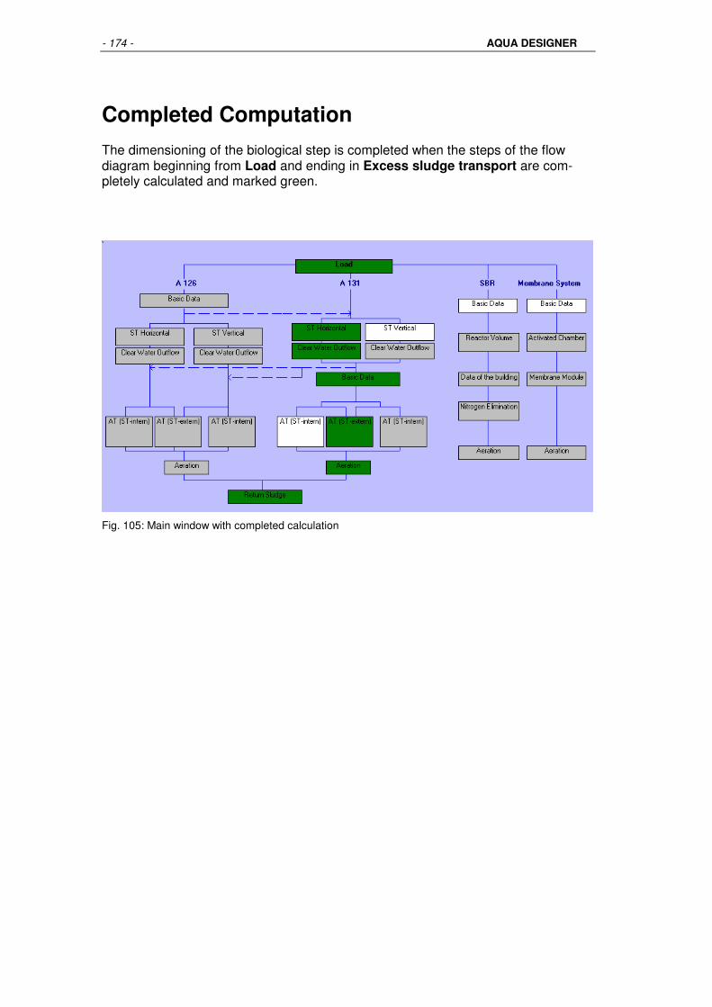
- 174 - AQUA DESIGNER
Completed Computation
The dimensioning of the biological step is completed when the steps of the flow diagram beginning from Load and ending in Excess sludge transport are com-pletely calculated and marked green.
Fig. 105: Main window with completed calculation

Dimensioning - 175 -
Grit Chamber Design
Circular and aerated Grit Chambers are included. Aerated grit chambers can be combined with grease chambers.
You reach the dimensioning site via Selection in the menu bar.
Dimensioning
Screen Grit and Grease Chamber
The screen is similar to the one known from the dimensioning of biological stages in AQUA DESIGNER.
You can make calculations for aerated grit chambers, grease traps, and circular grit chambers. The equipment components necessary for the dimensioning such as sand transportation, aerator, grease trap, and sand washer will be calculated or chosen.
After having finished the dimensioning you are able to calculate operating costs, to proof the calculation mathematically, to create an explanatory report, and to print drawings.
Fig. 106:Choosing of the screen Grease and Grit Chamber
Should you be on the screen for the biological stages you can reach the dimension-ing for the grit chamber via Menu > Selection > Grit and Grease Chamber.
Fig. 107: Screen for different kinds of grease and grit chambers

- 176 - AQUA DESIGNER
The documentation is at your disposal as soon as the calculations are made. As it is in the biological dimensioning the calculations for sewage treatment, operating costs, reports, and drawings can be found in the menu bar.
Circular Grit Chamber
The dimensioning of circular grit chambers is more specific to the producer than those of an aerated rectangular grit chamber. Sources in this field are sparse. The following publications a fundamentally based on the research from Kalbskopf from 1966.
Kalbskopf, K.H.: Die Bemessung von Sandfängen unter Berücksichtigung der Strö-mungsturbulenzen; Kommunalwirtschft 1966, Heft 9
The waste water is tangentially introduced into a round shallow funnel and flows horizontally through it. The circular stream creates a cross stream with a downward movement on the edges which drags down the desposited matter. The water level drops towards the centre of the circle while the horizontal flow velocity increases. The sand will be deposited in the centre of the funnel and can be centrally ex-tracted.
Fig. 108:Stream in Circular Grit Chamber
Dimensioning Basis
Kalbskopf
Input velocity: < 0.50 – 0.60 m/s
Outlet velocity: < 0.40 – 0.50 m/s
Theoretical retention period without sand accumulation area 30-45s
Outlet base approx. 10 – 15 cm higher than inlet base
With air lift pump: sand accumulation shaft depth = aeratio depth >= extraction height over water level + extraction length * 0.01

Dimensioning - 177 -
ATV Manual Mechanical Waste Water Treatment
Input velocity: < 0.75 – 1.0 m/s
Outlet velocity:< 0.80 m/s
Theoretical retention period without sand accumulation area 30-45s
Maximum input tR > 25s
Only one half of the truncated cone like grit chamber area is used to determine the hydraulic retention time. To simplify the calculations of the usable surface area an inner surface area is determined using half the diameter and is then substracted from the total surface area.
The funnel is designed for a complete dry-weather-flow. The water level only reaches the vertical or cylindrical part of the funnel if there is combined wast water flow.
The recommended funnel slope is 1 : 1.5.
A pile up can be achieved by introducing a following Venturi-channel.
Handling
You can predefine the number of lines. The waste water input will then be equally distributed to the chosen number of lines.
The sand accumulation shaft is shown on the control screen as being open down-wards. The depth of the shaft depends on the chosen sand extractor. The shaft will be deeper than the pumps if air lift pump is chosen. The diameter of the shaft is governed by the necessary area for the extracting machine, the diametral aeration system, and the desired sand storage capacity.
Fig. 109: Screen Circular Chamber

- 178 - AQUA DESIGNER
The screen will only be calculated when all steps are gone through. Only then will the results be processed for further steps.
Aerated Rectangular Grit Chamber
Aerated grit chambers can be constructed either with or without a grease and float-ing sludge channel at the side. Sand can be extracted through a suction device or a scrapper. The necessary air demand is governed by the basin‘s cross section area and length.
The calculation data is summarised below.
Fig. 110: Cross section of an aerated grit chamber
The dimensioning of aerated rectangular grit chambers with or without grease trap is based on the following literature.
ATV-Handbuch Mechanische Abwassereinigung
Abwassertechnische Vereinigung e.V., Bad Hennef Ernst & Sohn, Berlin, 1996
M. Boes, Anordnung und Bemessung der Luftzufuhr von belüfteten Sandfän-gen Korrespondenz Abwasser 7/90
A. Stein Ein Beitrag zur Gestaltung belüfteter Sandfänge Korrespondenz Abwasser 4/92
J. Londong Beitrag zur Bemessung belüfteter Sandfänge Korrespondenz Abwasser 1/88
ATV-Arbeitsbericht der ATV-Arbeitsgruppe 2.5.1 "Sandfänge" im ATV-Fachausschuß 2.5 Absetzverfahren Sandabscheideanlagen (Sandfänge und Sandfanggutaufberreitungsanlagen) Korrespondenz Abwasser 3/98
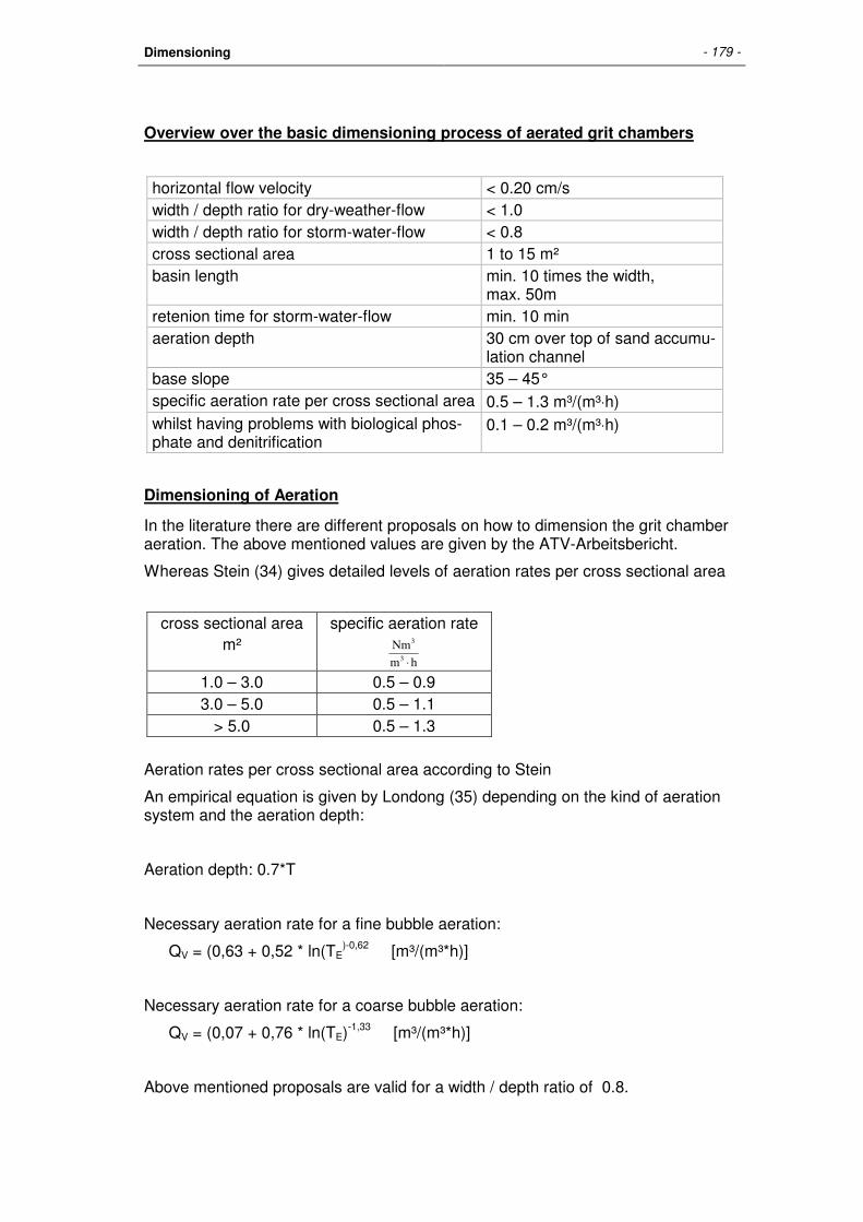
Dimensioning - 179 -
Overview over the basic dimensioning process of aerated grit chambers
horizontal flow velocity < 0.20 cm/s width / depth ratio for dry-weather-flow < 1.0 width / depth ratio for storm-water-flow < 0.8 cross sectional area 1 to 15 m² basin length min. 10 times the width,
max. 50m retenion time for storm-water-flow min. 10 min aeration depth 30 cm over top of sand accumu-
lation channel base slope 35 – 45° specific aeration rate per cross sectional area 0.5 – 1.3 m³/(m³⋅h) whilst having problems with biological phos-phate and denitrification
0.1 – 0.2 m³/(m³⋅h)
Dimensioning of Aeration
In the literature there are different proposals on how to dimension the grit chamber aeration. The above mentioned values are given by the ATV-Arbeitsbericht.
Whereas Stein (34) gives detailed levels of aeration rates per cross sectional area
cross sectional area m²
specific aeration rate
hm
Nm3
3
⋅
1.0 – 3.0 0.5 – 0.9 3.0 – 5.0 0.5 – 1.1
> 5.0 0.5 – 1.3
Aeration rates per cross sectional area according to Stein
An empirical equation is given by Londong (35) depending on the kind of aeration system and the aeration depth:
Aeration depth: 0.7*T
Necessary aeration rate for a fine bubble aeration:
QV = (0,63 + 0,52 * ln(TE)-0,62 [m³/(m³*h)]
Necessary aeration rate for a coarse bubble aeration:
QV = (0,07 + 0,76 * ln(TE)-1,33 [m³/(m³*h)]
Above mentioned proposals are valid for a width / depth ratio of 0.8.

- 180 - AQUA DESIGNER
Grease Trap
The ATV-Arbeitsbericht gives references on how to dimension a grease trap.
The width of the grease trap can be chosen to be about 0.2 to 0.5 times bSF.
A dimensioning depending on the surface loading rate is possible, too. The surface loading rate should then be <= 25 m/h.
Handling
You can predefine the number of Lines. The waste water input will then be equally distributed to the chosen number of Lines.
Fig. 111: Screen Rectangular Grit Chamber
The grease trap can be either chosen or not. That can be done by ticking the check box Grease Trap on or off. Should the grease trap be deactivated then there will be no channel at the side.
The basis for the data can be found above in this chapter.
The screen will only be calculated when all steps are gone through. Only then will the results be processed for further steps.
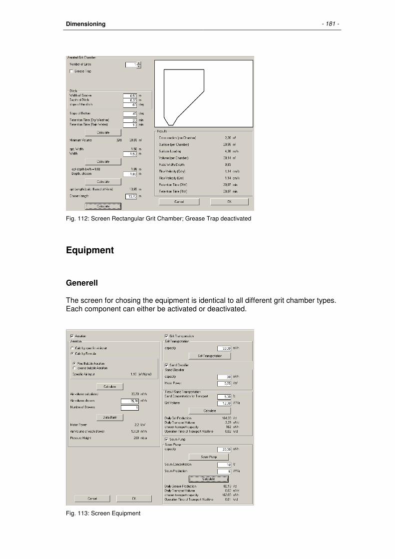
Dimensioning - 181 -
Fig. 112: Screen Rectangular Grit Chamber; Grease Trap deactivated
Equipment
Generell
The screen for chosing the equipment is identical to all different grit chamber types. Each component can either be activated or deactivated.
Fig. 113: Screen Equipment

- 182 - AQUA DESIGNER
Aeration
As mentioned in the dimensioning basis the aeration rate can be chosen either fol-lowing the ATV-Arbeitsbericht (36) or different empirical proposals. If the empirical proposal after Londong is chosen it can be further distinguished between fine and coarse bubble aeration.
First determine the necessary aeration rate.
You can then choose a fitting compactor from the data base.
Sand Extraction
First choose the sand extraction rate. The sand extraction rate is not calculated as being continuous, it will rather be done in intervals. The capacity of the sand extrac-tion device has to be chosen according to operational aspects. The extraction rate is mostly around 30m³/h.
Afterwards you can choose a compressed air lever, a fitting compactor, or a cen-trifugal pump respectively.
According to the chosen extraction rate, the calculated amount of sand and the con-centration of sand within the extracted material, a daily time of operation for the ex-traction device can be determiend.
Circular Grit Chamber
Aearation
Usually a circular aeration system will be situated within the pump pit of the circular grit chamber. This circular aeration system is loosening the sand on the bottom and cleans it of organic compounds.
The aearation ring is directly situated in the sand accumulation sump. The air leaves the ring through holes. The compressed air is introduced into the grit cham-ber by means of an air compressor.
The usual aeration rate of a circular grit chambers is approx. 30 m³/h.
The aeration can be done continuously in order to keep the water within the circular grit chamber fresh.
Yet, it makes sense to activate the aeration before the extraction process begins, in order to loosening the sand and cleaning it of organic compounds as described above.
Sand Extraction
For sand extraction both centrifugal pump and circular aearation system are possi-ble.
The rotors of centrifugal pumps are quickly worn, even if they are made out of hard-ened material.
More suitable for the sand extraction are compressed air levers. When using those the circular grit chamber has to be designed respectively, i.e. the aeration depth

Dimensioning - 183 -
should be no less than the extraction height plus 10% of the total extraction length. Therefore the sand accumulation sump has to be sufficiently deep.
Grease Separation
Circular grit chambers are ususally not designed to separate grease from the rest. Some separation can be achieved, though, e.g by introducing a scumboard at the outlet or certain constructions which are specific to the constructor. The grease is then pumped to a grease accumulation pit, from where the additional water has to be recirculated into the system.
Aerated Grit and Grease Chamber
Aeration
The geometry of the aeration is described within the dimensioning basis. Nowadays membrane aerators are used for the grit chamber aeration. They are put in row and line against the steep wall of the grit chamber.
Sand Extraction
The sand has to be transported to the sand accumulation sump at the top end of the grit chamber by a scrapper, or the collector pumps the sand-water-mixture di-rectly into the channel at the side of the grit chamber.
Sand Classifier
The sand will usually be seperated from the water in a sand classifier. The remain-ing water will then be recirculated into the system. When chosing the sand classifier it has to be taken care of that the capacity of the sand extraction device is not higher than the capacity of the sand classifier, i.e. that they have to have similar capacities. Should those capacities differ from each other, you will be notified.
Grease Extraction
Attached to the grit chamber cleaner is a grease plate, that transports the floating grease from the grease chamber into a grease accumulation pit. The grease is ac-cumulated in the upper section of the pit.´
Sand and Grease Volume
The absolute sand and grease volume can be calculated from the population equivalent and the chosen values for the specific sand and grease volume.
volumesand absolute365*1000
PE * volumesand specific=

- 184 - AQUA DESIGNER
volumegrease absolute365*1000
PE * volumegrease specific=
spec. sand/grease vol. volume after water separation l/(P*a) PE number of people P absolute amount amount after water separation m³/d
The extractable mixture volume can be calculated through the sand and grease concentration.
]d
m³[
10*c
amount absoluteQ
S/F
S/F =
QS daily sand-water-mixture output
d
m³
cS concentration of sand within the sand-water-mixture
%
5 % equals 50 kg sand per extracted m³

Databank - 185 -
DATABANK
In the databank the machines required for the operation of the wastewater plant are specified with their technical data and reference costs. Alltogether four different databanks for mixing devices, srew pumps, centrifugal pumps and blowers are available.
In the form Aeration the databanks for blower and mixing devices are available.
In the form Return Sludge the databanks for screw pumps, centrifugalpumps and air lift
pump blowers are accessed.
In the form Sludge Container a databank for selecting mixing devices is connected.
Clicking on DATA BANK in each of the above mentioned forms will open and give access to the databank.
When opening a databank a suitable machine is suggested selected according to specific criteria. The selection procedure for each databank is described below. Next to the databank window another window is placed displaying the relevant data for the selection of the according installation.

- 186 - AQUA DESIGNER
Fig. 114: Databank Window for Blowers with selected Installation
The recommended unit may be accepted or another unit may be chosen from the available selection.
Selecting another unit from the databank the directive keys are used. The outer buttons will bring you to the first and last available choice in the databank. The inner buttons will lead to the previous or next choice.
With the Search key the most suitable machine from the databank is selected by the program. This may be useful for returning to the original choice after browsing through the databank. Furthermore the last choice of the databank is selected with Search if no suitable installation was found.
You may ad data or installation choices respectively to the databank by clicking on New when no suitable installation is available from the databank.
An empty mask will appear for entering new data. Enter the key values of the cho-sen new installation into the according input fields.
Click on Save Data and to enter further choices select the appearing Further Data by clicking on Yes.
Again an empty mask appears to enter another set of data.
To leave this form by saving the last data set click on save data. The question Fur-ther Data appears. Click on No. You can also leave the form by Cancel. However in this case the last entered data are not saved.
Now the databank is automatically updated and the entered data sets are available for all future computations.

Databank - 187 -
Pumps
Left to the databank window the minimum requirements for the selection of the cor-responding pump are displayed. Here the transport capacity results from the re-quired total transport volume devided by the number of operating pumps.
Fig. 115: Minimum Required Values
AQUA DESIGNER will suggest an installation when the databank is accessed dur-ing the dimensioning. Primarily the program will take the transportation height into account and secondarily the transport volume.
Fig. 116: Specific Data for Pumps in the databank
The transportation height is the manometric transportation height. The Capacity is the maximum transport volume. It should be larger or equal to the previous dis-played transport volume.
The nominal motor power of the engine corresponds with the specification on the engine type plate. The power consumption is the power requirement at the opera-tion point.
The given type of pump enables you to find pump characteristics in a pump catalog.

- 188 - AQUA DESIGNER
Fig. 117: Pump Characteristics and Capacity
Mixer
For the sludge container and the activated sludge tank mixing devices are selected.
The required dimensioning data for selecting a mixing device or mixing devices re-spectively are displayed when accessing a databank window during the dimension-ing process.
AQUA DESIGNER will suggest a unit that is selected according to the nominal ca-pacity of the mixer engine. The mixer with the next in order nominal capacity is se-lected depending on the required energy input.
The recommended mixer may be accepted or another mixer may be chosen from the available selection.
The required energy input from the dimensioning is accepted for the power con-sumption.The investment costs are evaluated with this value.
Activated Sludge Tank
A specific energy input is suggested or selected by the user in the window Mixing Device of the Aeration form. The databank suggests an adequat mixing device for the chosen specific energy input. Choosing a smaller mixing device than necessary for the chosen specific energy input the required quantity of mixers is calculated automatically.
Example: The activated sludge tank volume is 1000 m³ and the specific energy input 3 W/m³. AQUA DESIGNER suggests a mixer with minimum nominal capacity of 3 kW after accessing the databank. Now choose a mixer with 1,3 kW nominal capacity. You will require at least three of the selected mixers to secure the required energy input. 3 * 1,3 kW = 3,9 kW > 3,0 kW For the following computation three mixers with each 1,3 kW are selected.

Databank - 189 -
Sludge Container
In the form Sludge Container a specific energy input is preselected or chosen by the user as well. The databank selects a mixing device with a nominal capacity meeting the minimum requirements for the energy input.
The user may select a smaller mixing device.
In contrast to the selection process in the form Aeration however, the number of mixers is not increased.
The dimensioning will still take only one unit into account selecting a mixer with a nominal capacity lower than the chosen energy input.
You may ad data or installation choices respectively to the databank by clicking on New when no suitable mixing device is available from the databank. An empty mask will appear for entering new data.
In the left window the required data from the computation are displayed.
The nominal capacity is the nominal capacity of the engine and is in accordance with the motor-type plate.
Technical Informations Usually slow rotating mixers are used in the biology. The diameter of the mixer is up to 2500 mm in these units with slow revolving propeller.
Blower
Blower are required for the aeration of the activated sludge tank and the return sludge transport.
In the dimensions considered here mainly rotary piston blower are used for the aeration. Compressors may be installed in small wastewater plants.
Predominantly compressors are used for the return sludge transport. This method of transport is particularly suitable for small plants.
Aeration
The quantity of blowers is entered in the Aeration form. The required total hourly air volume is devided by the number of blowers.
Clicking on Databank the databank opens for the selection of blowers for the acti-vated sludge tank aeration.
In the Value window the blower counter pressure and the required hourly air volume per blower is shown.
The counter pressure consists of the immersion depth and the aeration system losses.

- 190 - AQUA DESIGNER
The immersion depth is the water depth minus the installation level of the aerators. The installation level for the aerators is set as 30 cm above the tank base and a constructiv empirical value. The losses of the aeration system -pipe line losses and pressure losses of the aerator- are added with 150 mbar to the immersion depth.
Example: The water depth was selected as 4,8 m. The immersion depth is 4,5 m. This results in a counter pressure of 450 mbar. The pressure loss in the pipe line and aeration sysstem is 150 mbar. Thus the counter pressure for the dimensioning of the blower is 600 mbar.
Return Sludge Transport
Blower are available from the corresponding databank when choosing the option Air Lift Pump in the Return Sludge form.
Predominantly compressors are available for this application as air lift pumps are particularly suitable for small wastewater plants.
Compressors are economic for small air volumes.
Enter the number of blowers in the Air Lift Pump window. The required air volume is devided by the entered number of blowers.
Here the counter pressure results directly form the secondary sedimentation tank water depth (he = WT).
Primarily AQUA DESIGNER selects from the databank based on the counter pres-sure.
The introduction level for the compressed air should preferably be as deep as pos-sible for the most effective result. The pipe line losses are small.
Example: Having selected a tank with a water depth of 6,5 m in the Secondary Sedi-mentation Tank form a counter pressure of 6,5 mWS is displayed in the databank Required Value window. The databank selects a blower based on this value.
The selection is primarily based on the counter pressure and secondarily on the transport volume.
The power consumption is the power requirement at the operation point.
The given type of pump enables you to find pump characteristics in a pump catalog.

Menu Documentation - 191 -
MENU DOCUMENTATION
The design layout contains a complete documentation of the selected processes and chosen concepts.
It includes the description, the documentation of the computations and a summary of the operating and investment costs.
Fig. 118: Menue Design Layout
The design layout is prepared in a way that it is presentable as documentation or validation without requiring further editional work.
Please note that the text may be printed in English as well as German using the menue bar language option.
You will find the individual components of the design layout under the keyword Documentation in the menue.
Operation
Keys and Scroll Bars
Fig. 119: Buttons for display and output functions

- 192 - AQUA DESIGNER
Different keys are available to you in the design layout.
With the >> and << keys you can go forward and backward in the document.
A scroll bar is available for longer texts. Clicking on the scroll bar to the right of the screen will move the text vertically up or down.
Return to the Main Window clicking on OK.
Printing
You may instantly print individual design components by clicking on Print. In AQUA DESIGNER only the complete text will be printed for the Description and the calcu-lation of operating and investment costs.
Individual parts may be printed from the technical wastewater plant dimensioning. Choose Print from the menue bar located on the right. A window appears asking for Print All or Print Current Page. Choosing Print Current Page will print the current page on the screen. The complete technical wastewater computation will be printed with Print All.
The printer configuration can not be changed in the AQUA DESIGNER program. The printer settings should be on DIN A4, Portrait Orientation before starting to print. You can set up the printer configuration in another WINDOWS program e.x. Word or Excel or in the Print Manager.
Description
The selected wastewater plant concept is described in detail in the Description. The textblocks are assembled according to the Component Selection for the Pretreat-ment Step, Outflow and the operation building. These construction groups were not covered in the preceding computation process. They are to be selected separately. You will find the details in the chapter on ‘Extras’.
The description of the biological step is automatically assembled following the ac-cording computation. The according documentation will be presented in the descrip-tion depending on the selection of denitrification and phosphorus removal.
The Description is accessable with Design Layout > Description.
A title page for the description appears. The complete description may be printed on this page.
Clicking on Title Page will print a cover page for the complete design layout with description, technical wastewater plant computations and operation and investment cost evaluation.

Menu Documentation - 193 -
Dimensioning
The dimensioning is documented in detail in the calculation validation or the techni-cal wastewater plant computation respectively. The calculation steps are presented in detail to enable confirmation and validation.
Sections of the Technical Plant Dimensioning:
Basic Data
• Wastewater Inflow
• Loads
• Selected Concept
Biological Step
• Activated Sludge Tank
• Construction
• Oxygen Demand (Denitrification optional)
• Technical Equipment
• Heat Removal in the blower room
• Phosphorus Removal (optional)
• Secondary Sedimentation Tank
• Construction
• Technical Equipment
• Clear Water Outlet (Effluent Outlet)
• (Scaled) Drawing
Return Sludge Pump Station
• Excess Sludge Pump Station
• Sludge Treatment Construction
• Technical Equipment
The technical wastewater dimensioning documents the conducted computation in the AQUA DESIGNER program and thus, refers only to the biological step.
The technical wastewater dimensioning is accessable with Documentation > Di-mensioning.
The title page for the technical wastewater dimensioning appears.
- 194 - AQUA DESIGNER
Scaled Drawing
You can go directly to the scaled drawing with the Drawing key facilitating the re-view of the computation.
The drawing is a scaled drawing.
It is automatically and stepwise adapted to the page setting of the print
The drawings consist of a top view and section with construction measurements. The selected construction is presented in the drawing corresponding with the cho-sen construction type e.x. separate tanks, package plants, compact plants.
The display on the screen depends on the chosen screen view. The print automati-cally adapts to the chosen printer parameter.
The scale resulting from the adaption is shown.
Clicking OK on any page will bring you back to the Main Window.
Supplememtary Calculations
Additional calculations are conducted on the basis of the dimensioning data and documented in the technical wastewater dimensioning.
Industrial and Trade Components
Two different values are indicated for the concentrations of wastewater components in the basic data.
Initially the data are shown as entered in the form Basic Data viewing each single part of inflow.
The concentrations of the municipal, trade and industrial wastewater components are related to the Dry Weather Flow in the following table for Wastewater Inflow. Thus, the fraction of each component in relation to the total inflow is shown. The single concentrations in the table add to the total concentration of the corresponding components.
Air Exchange in the Blower Room
Care has to be taken for the room temperature not to rise too high when the blow-ersare installed within a building. The heat emission from the engines must be con-ducted off the room.
Part of the heat is transmitted off the room by the blowers that are constantly draw-ing in air from outside and transmit warm air into the activated chamber.

Menu Documentation - 195 -
If this process of heat removal is incomplete an additional Ventilator must be in-stalled that removes any remaining heat with an adequate airflow.
The radiated heat from the engines results from the (thermal) efficiency. A total of 15 % of the nominal capacity of the engine is set as heat loss.
The required air volume for heat removal is dependent from the specific heat capac-ity of the air and the density.
The required flow for the heat removal results to:
[ ]h
mdTrLcp
ePnnGQL
³*
3600***
+=
nG Blower Quantity Pn Nominal Capacity [kW] ε Heat Loss Share of the Motor Capacity cP Specific Heat Capacity [kJ/(kg * K)] ρL Density of Air [kg/l] dT Tolerated Temperature Increase
in the Blower Room [K]
The physical characteristics of the air -specific heat capacity cp and density ρ L - are taken from the VDI-Wärmeatlas /16/.
Physical Characteristics at 25°C and 1 bar:
cp = 1,007 [kJ/(kg*K)]
ρL = 1,168 [kg/m³]
It is possible to install the blowers outside a building. In this case no addi-tional heat removal is necessary. For small population equivalents the blowers are often sufficient to remove the produced air with the air flow for the biology. No ventilation is required in this case. It is not permitted to directly use the warm air from the blower room for the temperation of the screen room. This is prohibitted because the screen room is defined as hazardous area.
Pipelines
The siphon pipe from the activated sludge tank into the secondary sedimentation tank is designed for a maximum flow velocity of 0,5 m/s.
The outlet pipe is designed for a maximum flow velocity of 1,0 m/s.

- 196 - AQUA DESIGNER
Operating Costs
Choose description > operating costs from the menue bar. The title window op-erating costs opens.
Control Keys
Go back to the Main Window from any page with clicking on OK.
Return from the result display window to the basic data input fields for the operating cost calculation with the >> key.
Go directly to the window for entering the basic data for the operating cost calcula-tion with the << key. Changes in the calculation may be conducted fast with these keys.
Obtain a printout of the operating cost calculation with clicking on Print.
Choose >>. The windows for entering the basic data of the operating costs opens.
The calculation of the operating costs incorporates the energy costs, sludge and residual material disposal costs and the personnel costs.
The basic data for the operating cost calculation are entered corresponding with the selection of components and the dimensioning.
Only the operating costs for the biological step in accordance with the selected cal-culation method are evaluated when no additional components were chosen.
The basic data for the evaluation of the operating costs is entered one after another into three different forms. These forms correspond with the categorization of the operating costs.
Efficiency and delivery head for pumps as well as population equivalents of further Verbraucher are entered in the form Energy Consumption.
The amount of accumulating sludge based on empirical values and the dimension-ing is preselected for the form Sludge Disposal and Disposal Costs.
Labour requirements depending on the size of the wastewater plant and the design features are selected by the user in the Personnel form.
Energy Costs
Generell
Pump efficiency and delivery head is entered in the window Energy Consumption. The mean transport volumes are calculated based on the dimensioning.
Only the pumps for return sludge and excess sludge transport will be listed in the energy form when no additional components were selected.
Additional energy consuming devices are automatically shown when further con-struction groups were selected in the component selection.

Menu Documentation - 197 -
Pumping Stations
For the pumping stations:
• Inflow Pumping Station
• Intermediate Pumping Station
• Outflow Pumping Station
The delivery head must be reviewed individually and adapted manually as this value depends very much on the individual local conditions.
Technical Informations: In the inflow pumping station the mechanical step particularly the screen should be served evenly. Screw pumps are particularly suited for this purpose. Using centrifugal pumps in the inflow e.x. an even flow is enabled by frequency regulated engines. It is to be noted that unclarified wastewater is transported. The free passage of the pumps should be at least 100 mm. The pressure pipe should at least be selected as DN 100. A plant efficiency of 65 % may be assumed as directive value for pumping station with centrifugal pumps. Screw Pumps are particularly suitable to lift large water volumes over small height differences. Also they are suitable for the regular and even wastewater transport in the influent area. Using screw pumps for the return sludge transport is economical for large wastewater plants. Also the return sludge is transported with care, thus the activated sludge flocs stay intact and unbroken. A plant efficiency of 75 % may be assumed for screw pumps, if the operating point recommends the choise of this kind of pump. Air Lift Pumps are used for the return sludge transport. This method of transport goes with high operational costs. However, this is outweight by favorable invest-ment costs and a careful activated sludge transport in small plants. The air lift pump efficiency is around 45 %.
Combined (Sewer) System
The frequency of rain may be selected when the collector is constructed as com-bined (sewer) system. It determines the expected frequency of rain water occur-rence. This value is taken into account in the evaluation of energy costs for pumping.
A yearly precipitation of 600 - 1000 ml can be accepted for Germany depending on the climate area. In case of a rainstorm only the initial high loaded peak is collected and reduced in volume flow before entering the wastewater plant. In the event of continuous rain the storage tank will only refill the discharged amount. Thus the ratio of the combined sewerage inflow to the total wastewater inflow depends on the lenght of period of a stormrain event.
The rain frequency depending on the number of rain days is to be entered for the region where the wastewater plant will be located.#
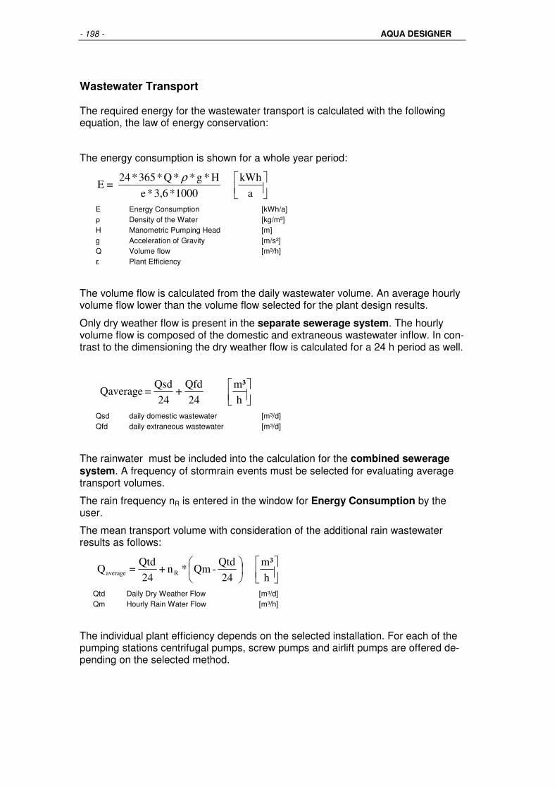
- 198 - AQUA DESIGNER
Wastewater Transport
The required energy for the wastewater transport is calculated with the following equation, the law of energy conservation:
The energy consumption is shown for a whole year period:
a
kWh
1000*3,6 * e
H * g * * Q * 365 * 24 = E
ρ
E Energy Consumption [kWh/a] ρ Density of the Water [kg/m³] H Manometric Pumping Head [m] g Acceleration of Gravity [m/s²] Q Volume flow [m³/h] ε Plant Efficiency
The volume flow is calculated from the daily wastewater volume. An average hourly volume flow lower than the volume flow selected for the plant design results.
Only dry weather flow is present in the separate sewerage system. The hourly volume flow is composed of the domestic and extraneous wastewater inflow. In con-trast to the dimensioning the dry weather flow is calculated for a 24 h period as well.
h
m³
24
Qfd +
24
Qsd = Qaverage
Qsd daily domestic wastewater [m³/d] Qfd daily extraneous wastewater [m³/d]
The rainwater must be included into the calculation for the combined sewerage system. A frequency of stormrain events must be selected for evaluating average transport volumes.
The rain frequency nR is entered in the window for Energy Consumption by the user.
The mean transport volume with consideration of the additional rain wastewater results as follows:
h
m³
24
Qtd-Qm * n+
24
Qtd = Q Raverage
Qtd Daily Dry Weather Flow [m³/d] Qm Hourly Rain Water Flow [m³/h]
The individual plant efficiency depends on the selected installation. For each of the pumping stations centrifugal pumps, screw pumps and airlift pumps are offered de-pending on the selected method.

Menu Documentation - 199 -
Other Installations
The energy costs for the other installations is evaluated depending on the operating time and the nominal capacity.
Mechanical Clarification
The size of the mechanical (preliminary) clarification correspond with the technical data of commonly used installations.
The operation period for the screen is preselected as 6 h/d based on an empirical value.
An operation period of 12 h/d is set when an aerated grit chamber is selected.
Air lift pumps transport the grit. The air lift pump is installed at the entrance of the grit chamber in the grit collecting channel. It resumes operation when the scraper reaches his start position. The operation period of the air lift pump is preselected as 2 h/d.
The operation period of the grit classifier corresponds with the air lift pump opera-tion period that is 2 h/d.
The grease separator operates 2 h/d as well.
The operation of the grit chamber scraper is initiated through a time program (oder: controlled by a time switch). An operation period of 3 h/d is assu med.
Commonly Square Grit Chambers have only a short aeration period for the grit aeration and a grit transport mechanism. Here an air lift pump is assumed for the grit transport.
The power consumption is preselected according to experiences with well known installations.
Biological Step
The rotary piston blower were selected from the databank during the dimensioning. There an aeration period was shown. The blowers were designed according to the air demand for the selected aeration period.
The blower output is generally slightly higher than the required air volume.
Furthermore the design oxygen load OB does not corresponds with the average oxygen load. In the design OB peak loads are included.
Mean oxygen load based on the ATV A131
The mean oxygen load is calculated based on the A131, however. the calculation does not include the peak loads or shock loads.
The shock factors fC and fN are selected as 1 in the equation for calculating the oxy-gen load.
Without shock factors OB, respectively OBSchmutzwasser is
In pure water:

- 200 - AQUA DESIGNER
5
2
NC
xs
s
purewaterkgBOD
kgO ) OU + (OU *
C - C
C = OB
In wastewater:
5
2purewater
wastewaterOB
OB = OB
kgBOD
kgO
α
The mean yearly water temperature is selected as 15°C.
The oxygen saturation concentration for saturated water vapor air and standard pressure (101,325 kPa) is described as a temperature dependent value only /1/.
m³
gO
45,93) + (T
2234,34 = C 2
1,31403theors,
Thus the oxygen saturation concentration in 15°C is 10,09 mg/l.
For intermittent aeration:
1,25 = 2,0 - 10,09
10,09 =
C - C
C
xs
s
Cs Oxygen Saturation Concentration mg/l Cx Operating Oxygen Concentration during
the Aeration Period mg/l
OUN is selected depending on the chosen clarification process of nitrification or de-nitrification. OUC as well as OUN are known from the dimensioning.
5
2
NCmittelkgBOD
kgO )OU + (OU *
Cx - Cs
Cs = OB
Mean oxygen load based on the ATV A126
A fixed mean OB is assumed for the evaluation of the blower operation period based on the A126. The mean OB is:
=
kgBOD
kgO 5,2
5
2
mittelOB
The daily air demand for the blower is calculated with the above evaluated mean OB. The average blower operation period results with the output capacity of the selected blower.
d
m³
hE*fO
1000 * B * OB = QL
2
BOD5d,mittel
Betrieb

Menu Documentation - 201 -
QLBetrieb Daily Mean Air Demand [m³/d]
The true blower operation period is lower than the operation period based on the dimensioning because of the above described operating conditions.
Blower Operation Period:
d
h
n * QL
QL= tL
GebläseGebläse
BetriebOperation
QLBlower Selected Blower Output [m³/h]
The blower power consumption is obtained from the databank.
AQUA DESIGNER allows the user to choose a blower with a lower than required capacity. In this case a notice to your attention appears in the Aeration form point-ing out the selection. In the calculation there is the possibility of a result of more than 24 h for the blower operation period if a much smaller blower is selected than suggested in the dimen-sioning process. In this event the operation period will automatically be fixed at 24 h/d. Only a maximum operation period of 24 h/d is possible for the blowers. This design corresponds with the operation reality. The tank aeration is insufficient when blowers of insufficient size are selected even with their continuous operation.
Operation Period of the Mixers
The mixers are usually operated continously. They keep the activated sludge in sus-pension during the unaerated period and ensure a complete mixing of wastewater and activated sludge. The additional circulation improves the oxygenintake during the aerated phase.
The power comsumption corresponds with the required energy supply in the dimen-sioning.
Sludge Treatment
The sludge tank mixer is operated only for short periods to improve the settleability of the sludge. The power comsumption corresponds with the required energy supply in the dimensioning and the operation period is 2 h.
The pump is designed for a default power of 1,5 kW and a daily operation period of 0,5 h. It is only required for the tank drainage.
The energy demand for pumping is listed at the pumping stations above.
The energy demand of the thickener and the mixing in the digester is based on ex-perience and literature, like /44/.
You are able to edit these values in the form.

- 202 - AQUA DESIGNER
Total Energy Costs
The yearly energy consumption for each installation is assembled and summarized in a table.
Enter the prize for energy in $/kWh into the Energy Consumption form.
The yearly energy costs result as a product from the yearly energy consumption and the specific energy prize.
Heat demand of the sludge treatment
The sludge treatment, especially the digestion itself needs a part of the produced heat for the digestion process. Therefor an average part of the produced heat is included in the energy balance. Its priced with the same tax as the produced heat.
Sludge Disposal
Different sludge types accumulate in the primary and biological treatment plant de-pending on the selected method of treatment.
In the preliminary treatment screenings and grit collect. Primary sludge from the primary sedimentation tank collects if a primary sedimentation tank was selected. Excess sludge from the biological step is collected and must be disposed of.
In the above form not all building blocks of a wastewater plant are included. All building blocks must have been previously selected in the component selection to obtain a complete assembly. The groups will automatically be displayed if they were already selected in the Description. In this form only the components resulting from the dimensioning will appear. This is the appearance when no additional components were cho-sen.
Fig. 120: Collected Sludge and Disposal Costs with individual groups

Menu Documentation - 203 -
Preliminary Treatment
Screen Contents
AQUA DESIGNER considers the volume of collected screenings when a screen was selected for the preliminary treatment in the component selection.
From experience in the wastewater plant operation an unpressed screenings vol-ume of about 32 l/(E*a) collects. Usually the screening step is followed by a screen-ings press to reduce the screenings volume to 16 l/(E*a). The suggested value may be altered by the user.
Information: The investment for a screenings press usually pays off fast as costs for disposal of screenings have become very expensive.
Grit
The collecting grit is considered in the operation costs if a detritor, an aerated grit chamber,a grease trap or a compact installation is selected in the component selec-tion.
The collected grit volume is classified and set as 16 l/(E*a). This value may be al-tered by the user.
Grit dewatering is not considered. In small wastewater plants container with bottom sieve screen and gate valves are used. In larger wastewater plants a grit classifier preceeds the container.
Grease
The collecting grease is considered in the operation costs when an aerated grit chamber and grease trap or a compact installation with grease trap is selected in the component selection.
Grease is usually separated in aerated grit chambers. The collecting grease is set as 6 l/(E*a) on the basis of wastewater pant operation experience. This value may be altered by the user.
Primary Sludge
The collecting primary sludge is considered in the calculation of the operating costs when a primary treatment is selected in the component selection.
The collecting primary sludge volume is set as about 40 l/(E*a).
Disposal Costs for Primary Treatment
Costs for the disposal of the screenings, grease and grit disposal come from ex-periences with costs for landfill disposal. The costs vary largely for different regions and we recommend for the user to inquire on the local costs for disposal.

- 204 - AQUA DESIGNER
Excess Sludge
The amount of collecting excess sludge results from the technical wastewater plant calculation.
The chemical sludge from the phophate precipitation is included in the indicated amount of excess sludge.
The relevant sludge volume for the operation costs results after the thickening in the sludge container.
The disposal costs in the window Sludge Disposal-Disposal Costs applies to agri-cultural disposal. These costs vary in different regions as well and should be in-quired locally.
Personnel Costs
The costs for personnel depend on the selected methods, the degree of automation and the wastewater plant size.
The report of the special ATV committee 2.12 for the operation of wastewater plants and personnel for the operation of wastewater plants (Arbeitsbericht des ATV-Fachausschusses 2.12 „Betrieb von Kläranlagen“ Personalbedarf für den Betrieb von Kläranlagen) includes recommendations for evaluating personnel requirements.
The report indicates the personnel requirements for wastewater plants serving population equivalents between 2000 and 250.000.
These costs should be evaluated with particular care as costs for personnel particu-larly in small wastewater plants may be of significant economic influence for a se-lected design.
The daily working period must be calculated from the working hours per week if the plant is not staffed daily.
E.x. a daily working period of 0,8 h/d results if the wastewater plant is staffed for half a day per week or 4 hours per week only.
The yearly costs for personnel are calculated as follows:
a
€
8
td * G * P = P ana
Pa Costs for Personnel €/a Pn Number of Staff Members Ga Yearly Salary €/a td Daily Working Time h/d

Menu Documentation - 205 -
Total Operation Costs
At the end the yearly operation costs consisting of energy costs, sludge disposal costs and costs for personnel are assembled and summarized.
The specific operation costs per population equivalent are shown in addition to the total operation costs.
Benefits from the Anaerobic Digestion
If an anaerobic digestion is part of the design, its possible to produve current and heat. Its assumed, that the current will be delivered to the power supplier by a fee. The heat can be used for the operation buildings. The fee of the current and the cost savings because of the use of the heat are listed at the end of the operating costs.

- 206 - AQUA DESIGNER
MENU EXTRAS
Components
Additional components like inflow pumping station or screens can be selected in case to complete the documentation and the operational costs.
All parts which are calculated and designed with AQUA DESIGNER are not part of the components list.
Sludge Treatment
The concept of sludge treatment depends on the kind of process of the water line.
If simultaneous aerobic sludge stabilization is chosen, its possible to dimension one or more sludge storage tanks.
If the water line is designed for separate sludge stabilization, tools for anaerobic sludge stabilization are available.
Fig. 121: Menu > Extras > Sludge Treatment
Thickener
Before treating the sludge, it should be thickened in a static thickener to 20 – 40 kg/m³.
The formular for the design of a thickener is available via Extras > Sludge Treat-ment > Thickener.
The thickener is simply designet for the retention time, oriented on the recommen-dations of Imhoff /44/.
You can edit the concentration after thickening at Options > Generel Constants > Sludge Treatment/Precipitants.
Also herefor you find recommendations at Imhoff: “Handbuch der Stadtentwässe-rung”/44/ and also in the ATV-“Handbuch Klärschlamm”.

Menu Extras - 207 -
Kind of Sludge Thickening Time
Possive DS-Concentrations
Raw Sludge 1 d 8,0 % Activated Sludge 1 – 5 % Sludge from Aero-bic Thermophil Sludge Treatment (ATS)
3 – 5 %
Mixed Sludge 3 – 7 %
The common device for thickening is the rabble rake. If you choose the rabble rake, its energy demand will be considered in the operating costs.
The anaerobic digester has to be feeded from the thickener. Therefor here you can select a progressive cavity pump. The energy for feeding will then also be consid-ered in the operating costs.
Fig. 122: Collected sludge and disposal costs with individual groups
The supernatant will also be considered in the total balances and is taken in ac-count for the internal flows.
Sludge Tank
For sludge treatment the storage in one or several sludge containers with gravita-tional thickening is planned.
Clicking on Menu > Extras > Sludge Treatment > Sludge Tank the form for di-mensioning the sludge container opens.

- 208 - AQUA DESIGNER
Fig. 123: Form Sludge Container
Sludge Detention Period
A sludge detention period of 90 d is suggested. This value may be altered in the corresponding input field by the user.
The sludge detention period depends on the wastewater plant size, the method of disposal and any further sludge treatment. A sludge detention period of 180 d is often demanded for small wastewater plants. A minimum period of 3 months - the nonvegetation time- has to be maintained for agricultural disposal. This corresponds with the above value.
The sludge detention period may be reduced depending on the operational re-quirements if a sludge dewatering process is planned. A common value for the sludge detention period is 20 d. This applies for a mobile mechanical sludge dewa-tering as well.
Thickening
Through sole gravitational thickening of aerobically stabilized sludge a maximum solids concentration of 5 % or 50 kg/m³ respectively is achieved.
Using preliminary dewatering processes (like centrifuges or drum sieves) the sludge is thickened to a value of about 8 %.
Adding flocculants increases the solids concentration.
Container Quantity
The construction of several containers is recommended for large wastewater plants. Operational advantages include the possibility of alternate loading of the containers and consequently the increase of the detention period for gravitational thickening.

Menu Extras - 209 -
Clicking on the first field for Calculate the required volume for each container is shown. Choosing two containers the displayed volume represents half of the re-quired total volume.
A diameter is preselected. Clicking on the second field for Calculate the corre-sponding water depth appears. Selecting a different diameter in the input field Di-ameter, selected the geometry of the sludge container may be altered.
Mixing Device
The contents of the sludge container are mixed in intervals to dissolve water accu-mulations in the sludge. A specific energy of 30 W/m³ applied by the mixing device is suggested for the above solids concentration and sole thickening of about 5 %.
This value is preselected in the window Mixing Device. It may be altered by the user entering another value in the input field Spec. energy input.
Choosing a lower specific energy for the mixing device is recommended for lower thickening rates selected by the user.
Clicking on Databank the databank for the mixing devices appears. The best matching mixing device from the databank is suggested.
See the chapter on databanks for details on databank function and operation..
Return to the Main Window with OK.
Anaerobic Sludge Digestion
Generell
Before calculating the sludge treatment, the water line has to be completed.
The instructions leaflet ATV-VDWK-M 368 defines the oeconomical limit for the an-aerobic stabilization of sludge at 10.000 – 50.000 population values /47/. Due to the changed funding situation through the subsidies for regenerative energy and con-stantly increasing energy costs it is necessary to check this evaluation. Due to the tendencies at the energy market the anaerobic stabilization of sludge is sure to eco-nomically efficient for ever-decreasing constructions. Withal the condition is, that the utilisation of gas occurs through a cogeneration unit (CHP) . It is really necessary to check this, resp. include it in planning, while choosing the anaerobic stabilization of sludge.
The treatment methods of the anaerobic stabilization of sludge are multifaceted. It involves as well the method of dewatering in single dewatering stages, as the rotting process and finally gas utilisation itself.
AQUA DESIGNER provides the basic scheme. With this basic scheme you can measure the single positions and receive sufficient exact information about the vol-ume of sludge and energy questions for the draft stage. The dewatering aims for preliminary dewatering; in most cases as static thickening or dewatering of the full-rotten sludge, usually through mechanical sludge dewatering, can be determined in the form General constants. In addition see the section Dry matter content some-what further below.
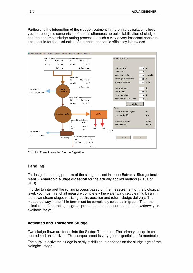
- 210 - AQUA DESIGNER
Particularly the integration of the sludge treatment in the entire calculation allows you the energetic comparison of the simultaneous aerobic stabilization of sludge and the anaerobic sludge rotting process. In such a way a very important construc-tion module for the evaluation of the entire economic efficiency is provided.
Fig. 124: Form Anaerobic Sludge Digestion
Handling
To design the rotting process of the sludge, select in menu Extras > Sludge treat-ment > Anaerobic sludge digestion for the actually applied method (A 131 or SBR).
In order to interpret the rotting process based on the measurement of the biological level, you must first of all measure completely the water way, i.e.: clearing basin in the down-steam stage, vitalizing basin, aeration and return sludge delivery. The measured way in the fill-in form must be completely selected in green. Than the calculation of the rotting stage, appropriate to the measurement of the waterway, is available for you.
Activated and Thickened Sludge
Two sludge flows are feede into the Sludge Treatment. The primary sludge is un-treated and unstabilized. This compartiment is very good digestible or fermentable.
The surplus activated sludge is partly stabilized. It depends on the sludge age of the biological stage.
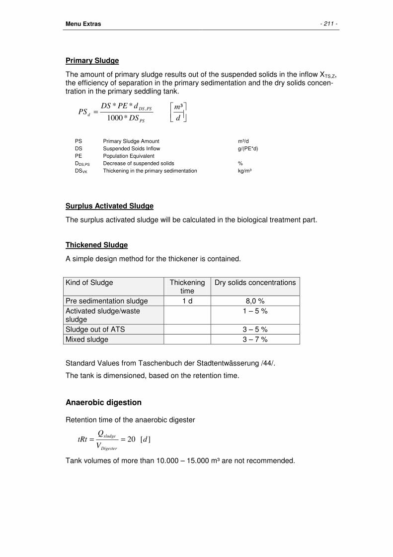
Menu Extras - 211 -
Primary Sludge
The amount of primary sludge results out of the suspended solids in the inflow XTS,Z, the efficiency of separation in the primary sedimentation and the dry solids concen-tration in the primary seddling tank.
=
d
m
DS
dPEDSPS
PS
PSDS
d
³
*1000
** ,
PS Primary Sludge Amount m³/d DS Suspended Soids Inflow g/(PE*d) PE Population Equivalent DDS,PS Decrease of suspended solids % DSVK Thickening in the primary sedimentation kg/m³
Surplus Activated Sludge
The surplus activated sludge will be calculated in the biological treatment part.
Thickened Sludge
A simple design method for the thickener is contained.
Kind of Sludge Thickening time
Dry solids concentrations
Pre sedimentation sludge 1 d 8,0 % Activated sludge/waste sludge
1 – 5 %
Sludge out of ATS 3 – 5 % Mixed sludge 3 – 7 %
Standard Values from Taschenbuch der Stadtentwässerung /44/.
The tank is dimensioned, based on the retention time.
Anaerobic digestion
Retention time of the anaerobic digester
][20 dV
QtRt
Digester
sludge==
Tank volumes of more than 10.000 – 15.000 m³ are not recommended.

- 212 - AQUA DESIGNER
Load Hydraulic Retention Time (tR)
d
Organic Dry Solids Volume Loading
dm
kgoTS
⋅³
Smaller Plants < 50.000 PE
20 2,0
Middle Sized Plants 50.000 – 100.000 PE
15 – 20 2,0-3,5
Large Sized Plants > 100.000 E
15 3,5-5,0
Table 4.2-10 /49/. Standard Values for digester design (summary)
For above recommended standard values the following conditions should be com-plied /49/:
• Municipal, pre thickened sludge, without specific industrial influence
• Primary Sludge without inhibiting compartiments
• Fermenter Temperature 35 – 37 °C
• Pre Heating of the sludge to fermenter temperature
• Mixing of the fermenter about 5 times per day and 20 operation hours per day
• Feed of the fermenter in multiple charges, minimum 3 charges per day
• With included rainwater treatment or chemical precipitation ann additional volume of 20 % is recommended.
Further to the retention time the organic volume loading should be verified. /44/
]³
[100
%*
100
%*
dm
kgoTR
V
GVDSQ
BRFF
rawsludge
rawsludge
⋅=
BRF = 2 – 3 kgorgTS/(m³xd) Middle sized plants kgorgTS/(m³xd) BRF = 2 – 3 kgorgTS/(m³xd) Large sized plants kgorgTS/(m³xd) BRF Organic volume loading kgOTR/(m³*d) GV Volatile, loss on ignition VF Volume Fermenter m³
Mixing
The specific power density for mixing has to be 5 – 15 W/m³, depending on the dry solids concentration in the tank.

Menu Extras - 213 -
Heating
To secure the process temperature of about 37 °C, the digester has to be provided with heat. This heat is usually produced out of the gas. An average value for the heat demand of the process will be 30 % of the produced heat.
Gas Production
An intensive mixing is important for good gas production. Also static conditions of raw sludge feeding and temperature are very important.
Kind of operation of the biological stage Organical Load Expected
biogas production 1. Sludge age activated chamber
(AC)tTS = 8 d (Nitrification in summer, partly denitrification)
Inflow activated stage 35 g BOD5/(PE x d) (large sized primary sed.)
Average: 20,7 l/(PE x d) Intervall: 16,5 – 25 l/(PE x d)
2. Sludge age (AC) tTS = 15 d (Nitrification and Denitrification)
Inflow activated stage 35 gBOD5/(PE x d)
Average: 18,3 l/( PE x d) Intervall: 10,5 – 15,9 l/( PE x d)
3. Sludge age (AC) tTS = 15 d
Inflow activated stage 48 gBBO5/(PE x d) (no primary sed.,rough desilting)
Average: 13,2 l/(Ewxd) Intervall: f10,5 – 15,9 l/( PE x d)
4. Sludge age (AC)tTS = 15 d
Inflow activated stage 60 gBOD5/(PE x d) (without primary sed.)
Average: 7,8 l/( PE x d) Intervall: 6,2 – 9,4 l/( PE x d)
5. Extended aeration min tTS = 25 d
Inflow activated stage 50 gBOD5/(PE x d) (without primary sed.)
Average: 4,4 l/( PE x d) Intervall: 3,5 – 5,3 l/( PE x d)
Table 5 /46/: Dependance of the expected biogas production from the process ofe wastwater
Recommended values for gas production:
/44/ Imhoff, 450 l/kgoMLSS
/47, DWA, 400 – 500 l/kgoMLSS
The energy content of biogas with 60 -70 Vol% Methan is about 6,0 – 7,0 kWh/m³. /46/ /49/
Separate Aerobic Sludge Treatment
Generell
The design is based on the leaflet ATV-DVWK-M 368 /47/ „Biologische Stabilis-ierung von Klärschlamm“. Two processes for separate aerobic sludge stablization are available. These are the Stabilization at environmental temperature and the sta-bilization at high temperature respectively aerobic thermophile sludge stabilization.
Operation, Handling

- 214 - AQUA DESIGNER
The separate aerobic sludge stabilization is available by the menu Sludge Treat-ment > Separate aerobic sludge stabilization > A131 or SBR. The menu ist only active if a waterline calculation A126, A131,SBR or MBR is completed.
Fig. 125: Menu seperate aerob stabilization
Primary and Surplus Sludge
The sludge treatment is feeded by to sludge flows. The primary sludge from the primary sedimentation is completely untreated and not stabilized.
The excess sludge or surplus sludge is partly stabilized. The degree of stabilization depends on the sludge age in the activated sludge system.
The primary sludge results of the settleable compounds in the inflow XTS,Z, the col-lection efficiency and the given dry solids concentration.
The following formula describes the primary sludge amount:
=
d
m
TS
dEWTSPS
VK
VKTSd
³
*1000
** ,
PS Primary Sludge m³/d TS Dry solids in the inflow g/(E*d) EW PE Population Equivalent dTS,VK Reduction of solids in the primary sedimentation % TSVK Thickening in the primary sedimenttation kg/m³
The excess sludge is calculated in the part of the activated sludge system.
Thickened Sludge
You can select the thickening of primary and surplus sludge. The degree of thicken-ing is determined in the menu general constants, because this value is also used in other parts of the program.
The degree of thickening can be edited separately for primary and surplus sludge. After the thickening the two sludge flows will be collected.

Menu Extras - 215 -
Fig. 126: Flows of thickening
Its recommded to thicken the primary sludge by sedimentation and the surplus sludge mechanical /47/.
Stuff Balance of Thickening
Fig. 127: Balance of thickining
Supernatant
QTW = QPS1 – QPS2 m³/d
d
m
TS
PS
TS
PSQ
PS
d
PS
dTW
³
21
−=
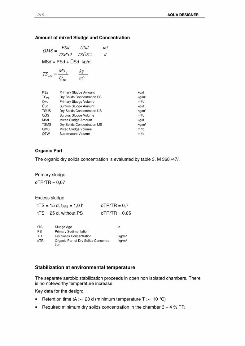
- 216 - AQUA DESIGNER
Amount of mixed Sludge and Concentration
d
m
TSÜS
ÜSd
TSPS
PSdQMS
³
22+=
MSd = PSd + ÜSd kg/d
³m
kg
Q
MSTS
MS
dMS =
PSd Primary Sludge Amount kg/d TSPS Dry Solids Concentration PS kg/m³ QPS Primary Sludge Volume m³/d ÜSd Surplus Sludge Amount kg/d TSÜS Dry Solids Concentration ÜS kg/m³ QÜS Surplus Sludge Volume m³/d MSd Mixed Sludge Amount kg/d TSMS Dry Solids Concentration MS kg/m³ QMS Mixed Sludge Volume m³/d QTW Supernatant Volume m³/d
Organic Part
The organic dry solids concentration is evaluated by table 3, M 368 /47/.
Primary sludge
oTR/TR = 0,67
Excess sludge
tTS = 15 d, tAPS = 1,0 h oTR/TR = 0,7
tTS = 25 d, without PS oTR/TR = 0,65
tTS Sludge Age d PS Primary Sedimentation TR Dry Solids Concentration kg/m³ oTR Organic Part of Dry Solids Concentra-
tion kg/m³
Stabilization at environmental temperature
The separate aerobic stabilization proceeds in open non isolated chambers. There is no noteworthy temperature increase.
Key data for the design:
• Retention time tA >= 20 d (minimum temperature T >= 10 °C)
• Required minimum dry solids concentration in the chamber 3 – 4 % TR

Menu Extras - 217 -
• Required aeration capacity OC >= 2,2 kgO2/(m³*d), for an oTR-degredation of 30 – 35 %
• Required power density for aeration and mixing NR >= 50 W/m³
Air Demand
h
m
WTfO
QMSOCQL
³
24**2*
*
α=
OC Oxygen Demand kgO2/(m³*d) QMS Volume of Mixed Sludge m³/d α Oxygen input factor, ca. 0,3 because of the
high solids concentration fO2 Oxygen input capability of the chosen
aerator gO2/(m³*m) WT Water level m
Thermophile Sludge Stabilization
Because of the exothermic degredation processes the sludge is heating up to 45 – 65 °C in isolated and covered tanks. At the higher temperature the degredation processes are running faster and you get a simultaneous disinfection.
Key data for the design:
• Retention time tA >= 5 d (minimum temperature T >= 10 °C)
• Required minimum dry solids concentration in the chamber ,53 – 6,5 % TR
• Required aeration capacity OC >= 2,2 kgO2/(m³*d), for an oTR-degredation of 30 – 35 %
• Required power density for aeration and mixing NR >= 80 – 180 W/m³
Air Demand:
h
m
tAO
VRCSBrohQL
³
24**2
***367,3*2,1
∆=
α
3,367 Conversion Factor m³L/kgO2 1,2 Safety Factor kgO2/kgCSBabg α CSB-Degredation CSBroh CSB-Concentration in Raw Sludge, ca. 1,6 kg/kg tA Stabilization Time d VR Reactor Volume m³

- 218 - AQUA DESIGNER
Load Variation
The oxygen transfer capability is described in the ATV M209 guideline. For pure water is the oxygen transfer capability specified in this text as the value is usually requested for analysis.
Oxygen transfer capability:
=
kWh
kg
P
OCOP
OC is the oxygen mass transferred into a pure water tank of given size within one hour by an aeration system at an oxygen concentration of C = 0 mg/l, a water tem-perature of 20°C and under standard pressure (atmospheric normal pressure of 1,103 hPa).
Oxygen transfer into pure water (20°C):
=
h
kgCskLaVOC
1000
20,*20*
kLa20 is evaluated when measuring the oxygen transfer.
Here the oxygen transfer capability is evaluated based on the design data. The oxy-gen transfer is calculated analogue to the calculation for the air demand.
The following applies to the air demand, calculated from the oxygen demand, in the case of fine bubble compressed air ventilation:
h
m
h * fO
1000 * OC = Q
3
E2
L
QL Required air volume per hour [m³/h] fO2 Oxygen transfer factor [g/(m³*m)] hE injection depth [m] OC Oxygen supply [kg/h]
The hourly air volune is established by the selected blower. The oxygen transfer factor (oxygen transfer capacity, fO2) is a characteristic value of the selected aera-tor. The expected operating value may be entered into the form for the oxygen transfer capability. The value does not need to meet the dimensioning value as that often is preselected comprising safety ranges.
Oxygen supply:
=
h
kghEfOQLOC Operation
1000
*2*

Menu Extras - 219 -
P is the power consumption of the aeration and the circulation units. It is useful to inquire about the power consumption of the circulation unit with the supplying com-pany as it usually differs considerably from the rated power. The power consump-tion of the blowers is known from the data bank.
Sludge Balance
The retention time of sludge in the secondary sedimentation depends on the sludge removal process and the return sludge flow.
Mainly there are two kinds of sludge removal devices, sludge scraper and suction devices.
Short-Circuit Sludge Flow
As the sludge removal flow rate QSR is oftgen smaller than the return sludge flow rate QRS, with sludge scrapers, a short-circuit sludge flow rate Qshort occurs be-tween inlet and sludge removal point (hopper) and wirth suction facilitiers from the zone above the thickening zone.
The following applies:
QShort = QRS – QSR [m³/h]
Solid matter balance:
QRS * SSRS = QSR * SSBS + QShort * SSEAT [kg/h]
Short-circuit sludge flow QShort:
h
m
SS
SSBSQrSSRSQRSQ
EAT
Short
³** −=
QShort short-circuit sludge flow in sedimentation hambers m³ / h QRS return sludge flow m³ / h QSR removal sludge flow rate m³ / h SSRS suspended solids concentration in return sludge kg / m³ TSBS suspended solids concentration in the bottom sludge of secondary
sedimentations kg / m³
SSEAT suspended solids concentration in the effluent of the biological reactor
kg / m³

- 220 - AQUA DESIGNER
Bottom Sludge and Return Sludge
Recommended thickening time:
• Activated chamber without nitrification: 1,5 - 2,0 (te in h)
• Activated chamber with nitrification: 1,0 - 1,5 (te in h)
• Activated chamber with denitrification: 2,0 - ( 2,5 ) (te in h)
The sludge removal device has to designed so, that the thickening time not will be exceeded.
Suspended solids concentration in bottom sludge:
The decrease of concentration because of short circuit sludge flow will be taken into account by the removal factor:
• scraper : SSRS ca. 0,7 * SSBS
• suction device: SSRS ca. 0,5 - 0,7 * SSBS
Pipelines
Choose Extras > Pipelines.
The diameters of the pipelines are calculated based on the flow velocity. Its not an hydraulical calculation.
The flow velocities for the evaluation of the pipeline diameters are available at Generell Constants in the folder Buildings/Equipment. In the frame Flow Velocities you can edit the velocity for water and air.
Water Pipes
The connecting pipelines between the treatment building have to be designed for various water flows. The flow in the return sludge pipes depends on the return sludge ratio. The pipeline between activated chamber and secondary sedimentaton has to transport the inflow and the return sludge.
Air Suport Pipelines
The air support pipeline system is usually very ramified. Here you get a list of the various diameters.

Menu Extras - 221 -
1 Connecting Pipe
2 Collecting Pipe
3 Ring Pipe arround a chamber
4 Pipe to the aeration devices
Fig. 128: Air supply pipeline system
Oxygen Efficiency
The oxygen efficiency is described in the ATV Paper M 209 /23/. Further information will be found at Wagner /28/.
Here the oxygen efficiency in pure water will be evaluated, because this parameter usually has to be verified.
Definition
=
kWh
kg
P
OCOP
Also declared as SAE, Standard Aeration Efficiency.
OC is the amount of oxygen, which should be solved from a oxygen concentration C = 0 mg/l, at a water temperature of 20 °C at an atmospharical pressure of 1,103 hPa within an hour into a chamber of a defined size, filled with pure water.
=
h
kgCskLaVOC
1000
20,*20*
Kla20 will be evaluated by the oxygen input measuring.
Membrane Aeration
AQUA DESIGNER evaluates the oxygen efficiency based on the design values. The oxygen supply will be calculated like in the calculation of the oxygen demand.

- 222 - AQUA DESIGNER
Fig. 129: Oxygen Efficiency
Air demand, evaluated from the oxygen demand:
h
m
h * fO
1000 * OC = Q
3
E2
L
QL Hourly Air Supply [m³/h] fO2 Oxygen Transfer Capability [g/(m³*m)] hE Immersion Depth [m] OC Oxygen Demand [kg/h]
The hourly air supply is defined by the selected blowers. The oxygen transfer capa-bility is a parameter of the aeration device. The value in operation can be defined in the formular Oxygen Efficiency. It can differ from the design value, because often the design value is chosen with security factors.
Oxygen Input:
=
h
kghEoperationfOQLOC
1000
*2*
P is the power consumption of the blowers and mixers. For the mixing devices its recommend to request the aggregats by a supplier to get detaild values for the power consumption. The power consumption of the blowers is known out of the data bank. Mechanical losses and the efficiency of the motor are considered.

Menu Extras - 223 -
Blowers
The coupling power is known out of the data bank. Mechanical losses are consid-ered by a value of 5 %. Also important is the efficiency of the motor. At 5,5 kW you can assume an efficiency of about 83 %. At 100 kW motor power the efficiency is about 95 %.
The power consumption can be estimated by
Motor
Coupling
elA
PP
η
05,1*, =
Following you find some average values of the motor efficiency of roots blowers.
2-pole Motors (3000 min-1)
Nominal power kW
4,0 11,0 45,0 110 500
Efficiency % 83 87 93,7 95,4 97
4-pole Motors (1500 min-1)
Nominal power kW
4,0 11,0 45,0 110 500
Efficiency % 83 86 93 95,1 96,8
Surface Aeration
At Wagner /28/ you will find experimental evaluated models for the different aeration types.
Oxygen efficiency of horicontal axis aerators (rotors)
=
kWh
kgO2LD * 0,0058 - 1,97 ON10
Oxygen efficiency of vertical axis aerators in plug flow reactors
=
kWh
kgO2LD * 0,0121 - 2,36 ON10
(not statistical verfied)
Oxygen efficiency of vertical axis aerators in mixed reactors
+=
kWh
kgO2LD * 0,0055 1,41 ON10

- 224 - AQUA DESIGNER
Mixing
If Mixers are selected, the power will be considered in the oxygen efficieny. Be-cause the power consumption of the mixing will not be calculated in AQUA DESIGERN, here the nominal power is taken into account. If the power consump-tion is known by the suppliers data, you can enter this value into the input field Power Consumption per Mixer.

Menu Drawing - 225 -
MENU DRAWING
The true scaled drawings are a powerfull component of AQUA DESIGNER to verify the way of design and to add drawings to your documentations. For an experienced engineer, the drawing will show immediately while calculating, wether the design is matching to his demands and all aspects are accurately.
The mass calculation and bouyancy supports you with additional information to proof oekonomical aspects or to hand out additional information for the tendering.
Drawings
Clicking on Drawings > Drawings > A126/A131 the form for editing the true scaled drawings opens.
Fig. 130: Menu Drawings
If you have designed separated chambers for sedimentation and activated cham-ber, an intermedient form will occur. Here you have to decide what chamber you want to display.
Fig. 131: Form Intermediate form for chosing activated or sedimentation chamber
Here for example, you want to see the activated chamber.
After clicking OK the form for editing the drawings will occur.

- 226 - AQUA DESIGNER
Fig. 132: Form drawings for activated chamber
Fig. 133: Form drawings for compact chamber system
You are able to edit the true scaled drawings directly in AQUA DESIGNER. As the dimensions of the chamber are results of the design, these values are fixed. The diameter of the chambers cannot be changed after finishing the design. Also, if you
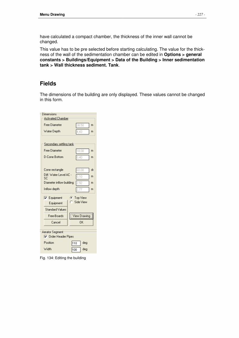
Menu Drawing - 227 -
have calculated a compact chamber, the thickness of the inner wall cannot be changed.
This value has to be pre selected before starting calculating. The value for the thick-ness of the wall of the sedimentation chamber can be edited in Options > general constants > Buildings/Equipment > Data of the Building > Inner sedimentation tank > Wall thickness sediment. Tank.
Fields
The dimensions of the building are only displayed. These values cannot be changed in this form.
Fig. 134: Editing the building

- 228 - AQUA DESIGNER
Fig. 135: Form for oxidation ditch
Middle Wall The middle wall can be inactivated. After inactivating, the middle wall will be removed.
Equipment The aeration system and the mixers are displayed in the drawing, for example to verify wether the dimensions are fitting to the size of the chamber. By inactivating the label Equipment, only the building will be drawn.
Buttons Values to be edited are available by the buttons Equipment, Stan-dard Values and Free-Boards.
Equipment
Distance to Wall Distance of the lattice to the outer ring wall. Distance of the Tubes Distance between the aerator tubes, fixed on the header pipes. Distance of Discs As before for aeration discs Mixers Its strongly recommended to let enough space betwenn the mixer and the aeration equiment. This space can be edited here.
Free Boards

Menu Drawing - 229 -
Standard Values
Thickness Wall Activated Chamber Outer Wall of an activated or combined chamber system.
Wall thickness sedimentation tank Outer wall of a sedimentation tank, or inner wall of a combined chamber sys-tem. In combined chamber systems this value can only be edited before starting the calculation in the form general con-stants.
Diameter Sludge Cone
Width or the Spur
WxL low point
At the low point you can dewater the chamber.
Order Header Pipes

- 230 - AQUA DESIGNER
Membrane Aeration System
After calculating the oxygen and air demand for surpressed air systems and select-ing blowers ander mixers, the aeration and mixing system is displayed inside of the activated chamber also as true scaled drawing.
Fig. 136: Activated chamber aeration system
Fig. 137: Combined chamber system, aeration placement

Menu Drawing - 231 -
The form opens in Top View modus. The properties of the aeration system can be edited on the left side. At the bottom part of the form, a detailled drawing of one aeration lattice is displayed.
Control Picture
At the calculation step for the sedimentation tank and at the activated chamber you are able to view the design of the chamber.
After calculating a sedimentation chamber or an activated chamber press the button Control Picture.
A true scaled drawing of the chamber will appear.
You are able to display as top view or side view.
Output of Drawings
You are able to Print the drawings, or to export them as a DXF-File.
For output of the drawings you have to open the form drawings with Drawings > drawing or with Control Picture or in Membrane Aerator.
After the drawing is displayed on the screen, select Drawings > View Drawing > Print or DXF.
Fig. 138: Menu for output of drawings

- 232 - AQUA DESIGNER
Mass Calculation
Before calculating the masses of concrete and excavation you may edit the draw-ing. The masses are based on the chosen values for wall thickness, spur and free boards.
Clicking on Drawing > Mass Calculation > A126/A131 the form for mass calcula-tion opens.
Fig. 139: Form for mass calculation
Only the values for the Slope of the Pit and the Work Space has to be selected. Then, all information for calculating concrete and excavation is provided.
Fig. 140: Pit for activated chamber

Menu Drawing - 233 -
Fig. 141: Pit for a compact chamber, Neigungswinkel = Slope, Arbeitsraum = Work Space
Bouyancy
Before calculating the bouyancy for a chamber you may edit the drawing. The masses are based on the chosen values for wall thickness, spur and free boards.
Clicking on Drawings > Bouyancy > A126/A131 the form for bouyancy opens.
Fig. 142: Form for calculation of bouyoncy

- 234 - AQUA DESIGNER
The weight of the technical equipment will not be considered.
The bouyancy will be calculated based on the mass of the building. The resulting permitted ground water level is ment for an empty chamber.
If there is chosen a spur, the concrete of the spur and also the soil mass on the spur is considered for the mass of the chamber.
The friction rectangle depends on the properties of the soil.

Verifying - 235 -
VERIFYING
With the help of the Recalculation menu you are able to assess the actual (theoreti-cal) capacity of the currently operating wastewater plant or of parts of the plant.
Fig. 143: Menu > Verify
The actual capacity of many of the existing plants is not known as they were dimen-sioned on the basis of currently outdated regulations. It is, therefore, necessary to recalculate the plant capacity on the basis of the most current regulations for any expansion or addition of lines.
For this purpose, the previously demonstrated dimensioning process is reversed. This means that based on the evaluated dimensions, the permitted charges and loads are recalculated.
AQUA DESIGNER enables you to recalculate different tank variations on the basis of the ATV guideline A131 and A126.
Secondary Sedimentation Tank
It is possible to recalculate existing sedimentation chambers based on the ATV guidelines A126 and A131. The data for dimensioning the surface area and the wa-ter depths are entered first. The permitted hydraulic load of the existing chamber is calculated from the selected MLSS for the activated sludge chamber, the return sludge ratio and the data for the sludge characteristics.
Calculation
Surface Area
You have the choice of circular, rectangular or hopper-bottom tanks.
Choose Other Tanks and enter a surface when the existing type of tank is not listed.
Flow
You can choose the Vertical or Horizontal Flow option for recalculating an existing circular chamber.

- 236 - AQUA DESIGNER
For a deep sedimentation chamber, it is useful to examine the possibility of calculat-ing a vertical flow sedimentation.
Choose Vertical Flow in the Flow window to calculate this variation.
The present sedimentation chamber will now be considered a vertical flow sedimen-tation tank. The sludge volume loading is preselected as 650 l/(m²*h). AQUA DESIGNER calculates the inflow depth in accordance with the applicable guideline and examines the feasability of vertical flow for the chamber. If the preconditions for a vertical flow tank are not satisfied, AQUA DESIGNER will not continue with the computation. At this point, change to the Horizontal Flow option to continue the calculation.
Fig. 144:Existing Circular Chamber
For a horizontal flow sedimentation tank the sludge load volume is preselected as qsv = 450 l/(m²*h).
A hopper-bottom tank is calculated as vertical flow chamber by the program.
Rectangular tanks and tanks entered into the Other Tanks option are calculated as horizontal-flow chambers.
For rectangular sedimentation tanks the disturbing or inlet zone is not included into the effective surface area. According to the ATV, the water depth will be suggested as length of this zone. Please see the part on Secondary Sedimentation tanks as Rectangular Tanks in the Dimensioning Chapter as well.
Water Depth
The peripheral water depth and the water depth at the central inlet is required for calculating the secondary sedimentation tank slope. The slope and the total depth at 2/3 of the flow distance are calculated from the peripheral and central water depths.
Central Inlet
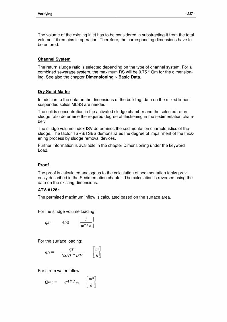
Verifying - 237 -
The volume of the existing inlet has to be considered in substracting it from the total volume if it remains in operation. Therefore, the corresponding dimensions have to be entered.
Channel System
The return sludge ratio is selected depending on the type of channel system. For a combined sewerage system, the maximum RS will be 0.75 * Qm for the dimension-ing. See also the chapter Dimensioning > Basic Data.
Dry Solid Matter
In addition to the data on the dimensions of the building, data on the mixed liquor suspended solids MLSS are needed.
The solids concentration in the activated sludge chamber and the selected return sludge ratio determine the required degree of thickening in the sedimentation cham-ber.
The sludge volume index ISV determines the sedimentation characteristics of the sludge. The factor TSRS/TSBS demonstrates the degree of impairment of the thick-ening process by sludge removal devices.
Further information is available in the chapter Dimensioning under the keyword Load.
Proof
The proof is calculated analogous to the calculation of sedimentation tanks previ-ously described in the Sedimentation chapter. The calculation is reversed using the data on the existing dimensions.
ATV-A126:
The permitted maximum inflow is calculated based on the surface area.
For the sludge volume loading:
=
hm
lqsv
*²450
For the surface loading:
=
h
m
ISVSSAT
qsvqA
*
For strom water inflow:
=
h
mAqAQmz NB
³*

- 238 - AQUA DESIGNER
Hints
A hint appears when an existing horizontal flow sedimenation tank can also be cal-culated as a vertical flow chamber. This is the case for an inflow depth larger than half the horizontal flow distance.
A hint appears when the vertical flow option has been selected and the condition of inflow > flow distance/2 is not fullfilled. The program will not allow you to continue the calculation with the vertical flow option.
A hint appears when the conditions for minimum depths are not guaranteed. Again the program will not allow you to continue the calculation.
The following minimum depths are required:
Peripheral Depth: >= 3.5 m
Total Depth: >= 4.0 m
Hopper-bottom Tanks:
Height Cylinder: >= 1/3 Height Cone
Height Cylinder >= 2.0 m for separated sewer system
Height Cylinder >= 3.0 m for combined sewer system
ATV-A131
The levels of the sedimentation chamber liquid zones for the present sedimentation chamber are evaluated using an iteration with qsv and qA until the total depth cor-responds with the liquid level zones.
The sludge thickening time and the sludge concentration factor are calculated on the basis of the entered values for the MLSS in the activated sludge chamber, the return sludge ratio and the sludge volume index.
+=
³
*
m
kg
RV
RVSSSSSS ATAT
RS
=
³/ m
kg
SSBSSSRS
SSRSSSBS
[ ]hISVSS
tE BS
3
1000
*
=
C = 300 * tE + 500 [kg/m³]
The maximum qsv is 450 l/(m²*h) for the horizontal flow sedimentation and 600 l/(m²*h) for the vertical flow sedimenation.

Verifying - 239 -
A hint appears when an existing horizontal flow sedimenation tank can also be cal-culated as a vertical flow chamber. This is the case for an inflow depth larger than half the horizontal flow distance.
A hint appears when the vertical flow option has been selected and the condition of inflow > flow distance/2 is not fullfilled. The program will not allow you to continue the calculation with the vertical flow option.
A hint appears when the conditions for minimum depths are not guaranteed. Again the program will not allow you to continue the calculation.
The following minimum depths are required:
Peripheral Depth: 2.5 m
Total Depth: 2.0 m
Activated Sludge Chamber
Existing activated sludge chambers can be recalculated following the guidelines A131 and A126 of the ATV. The calculation inludes the permissible BOD5 load and the required air volume and aerator length resulting from the water depth and the aerator loading.
Fig. 145: Inputs for the dimensioning according to A131

- 240 - AQUA DESIGNER
Guideline
A126
Bd,BOD5 = BR * VAT [kg/(kg*d)]
A131
In the A131 guideline, the sludge age is the basis for the recalculation analogous to the dimensioning of a new wastewater plant. In the A126 guideline the sludge vol-ume loading is the basis for the recalculation. The phosphate removal process may be considered as a basis for recalculating an existing activated sludge chamber.
The biological excess sludge production is iterated.
WSBOD5 = f(SSo, BOD5, tts)
The calculation for the chemical excess sludge production from phosphate precipi-tation was described before in the Dimensioning chapter.
The sludge load is calculated as:
=
dkg
kg
tTSWSBBSS
*min*
1
BR = BTS * SSAT [kg/(m³*d)
Bd,BOD5 = VAT * BR [kg/(kg*d)]
The true sludge age is calculated after entering the selected BOD5 load in the ac-cording input field. The aeration system is calculated using the calculated sludge age and the selected BOD5 load.
Type of Tanks
Circular chambers, rectangular chambers and ring chambers with central sedimen-tation are available. Ring chambers are the activated sludge chamber part of a com-pact system with the activated sludge chamber arranged around a central secondary sedimentation tank.
Compact systems with central hopper-tank are not available. To calculate this varia-tion enter the volume of the activated sludge chamber into the according field in the option Other Tanks.

Verifying - 241 -
Phosphate Removal
A phosphate outflow limit value can be taken into account in the calculation.
A calculation that includes a phosphate removal process is available in the A131 guidelines only.
Select Phosphate Removal by clicking on the according control box. A window Phosphate Removal appears, analogous to the window in Basic Data.
The suggested or selected anaerobic volume will be substracted from the total acti-vated sludge tank volume. It is not included into the evaluation of the permissible BOD5 load.
Aeration
Oxygen demand, air demand and aerator length are calculated analogous to the calculation for a new wastewater plant after the BOD5 load of the existing activated sludge tank has been evaluated. See the chapter Dimensioning - Aeration for the calculation of the oxygen supply.
Fig. 146: Left: Basic Data for the calculation of oxygen- and air demand according to A131; Right: Data for the nutrient balance
The selected BOD5 load and the resulting sludge age are the basis for calculating the oxygen and air demand of an existing activated sludge tank.

- 242 - AQUA DESIGNER
MENU OPTIONS
Several tools are available from the menu Options that increase the flexibility of the calculations. Also there is the possibility to change the working language and lan-guage for print outs.
Language
Click on Menu > Options > Language and choose one them.
If you change from a CE (central european)-font to the chinese or the cyrillic font, you first have to activate the according font on your PC and to make a new start of your PC.
Fig. 147: Menu > Options > Language
Settings
Click on Menu > Options > Settings. A formular to choose different parameter for the calculation process or the documentation appears.
Options
Multiline
Clicking on Multiline the program allows you to calculate several parallel lines in the biological step. Selecting Multiple Lines the option is marked.

Menu Options - 243 -
Fig. 148: Menu Options > Settings
Intermediate windows will appear for the Multiple Lines and the Incorporating Existing Plant Components in the Options asking you for the number of lines to be installed for the secondary sedimentation tanks or the activated sludge tanks.
Secondary Sedimentation Tank
Select a sedimentation chamber by clicking on the according field after completing the Basic Data form. If the Multiple Lines option has been selected, an intermedi-ate window will appear. Here the desired number of parallel lines or chambers is entered.
Clicking on OK, the familiar form for calculating secondary sedimentation chambers will appear.
All data in this form are linked with one secondary sedimentation chamber. The di-mensioning is based on the wastewater inflow volume for one line.
It is only possible to calculate parallel lines of the same size.
Preexisting lines that are incorporated into the dimensioning may differ from the size of new constructed lines.
Activated Sludge Tank
Enter the desired number of parallel lines or chambers into the field Number of Activated Sludge Chambers of the intermediate window. In the form for the di-mensioning of activated sludge chambers one chamber is calculated only based on the load for one line. All data in this form are linked to one line or one chamber.

- 244 - AQUA DESIGNER
Aeration
The oxygen demand and required air volume is calculated for the entire wastewater plant and displayed accordingly.
Blower
The number of blowers for the entire wastewater plant is listed in the field: Number of Blowers. The default value is set for two blowers for each line. You may enter any number of blowers. For example 8 blowers are suggested by AQUA DESIGNER when choosing 4 lines. It is, however, possible to set 3 blowers for 4 lines. The total capacity of all blowers chosen from the databank will be equally dis-tributed over all the lines.
Mixer
One mixer is selected for each line. The number of mixers entered must be divide-able through the number of lines. For example you will enter 4, 8, 12 or 16 mixers when choosing four lines.
Aeration
In the Aeration form all the values are based on one sedimentation tank only. Also the result display for one aeration screen in the lower right window is calculated for one sedimentation tank only.
Considering existing plants
Existing plant components may be incorporated into the calculation of new lines or the expansion of an existing plant.
Click on Options > Incorporate Existing Plant Components
An intermediate window appears in the main window after clicking on Secondary Sedimentation Tank and Activated Sludge Tank as before with choosing the op-tion Multiple Lines.
Sedimentation Tanks
Click on (Re)Calculate Existing (Secondary Sedimentation) Tank in the Existing Sedimentation Tank window. You can recalculate an existing secondary sedimen-tation tank with this procedure and include the result into the design.

Menu Options - 245 -
Fig. 149: Intermediate windows for taking existing sedimentation tanks into account
Operational instructions for the Recalculation forms were previously available in this chapter under the keyword Recalculation.
Values like the sludge volume index or the return sludge ratio that were entered previously into the form Basic Data will be only displayed in this section and cannot be changed anymore.
The resulting hydraulic load is displayed in the form Recalculation. You may accept the displayed result in the field Selected Combined Wastewater Inflow (Qmz) or enter another value. For example, it may be helpful to enter half the hydraulic load at this point when the construction of a second line of the same size is planned.
The value entered in the field for Selected Combined Wastewater Inflow (Qmz) is incorporated into the computation and deducted from the total inflow. The dimen-sioning of one or more secondary sedimentation tanks is conducted with the re-maining inflow.
The remaining inflow will be divided by the the number of selected lines when Mul-tiple Lines were selected. Therefore, it is possible to incorporate an existing tank into the computation or calculate an expansion with an increase in the number of lines.
Activated Chamber
Similar to the dimensioning of the sedimenation tanks you can incorporte an exist-ing activated sludge tank in the dimensioning of the activated sludge chamber. Val-ues previously entered in the form Basic Data cannot be changed at this point.
The BOD5 load of the existing plant will be substracted from the total BOD5 load. The new chambers/tanks will be dimensioned for the remaining BOD5 load.
Aeration
Calculating the oxygen intake and supply there is again the choice of only calculat-ing the capacity for an existing plant or to calculate the required aeration capacity for the total load of a new plant.
Clicking on the control box as demonstrated in the picture above, the fraction of the existing plant will not be included in the calculation for the new plant.
Leaving the control box blank, the aeration for the new activated sludge tanks is calculated based on the total load.
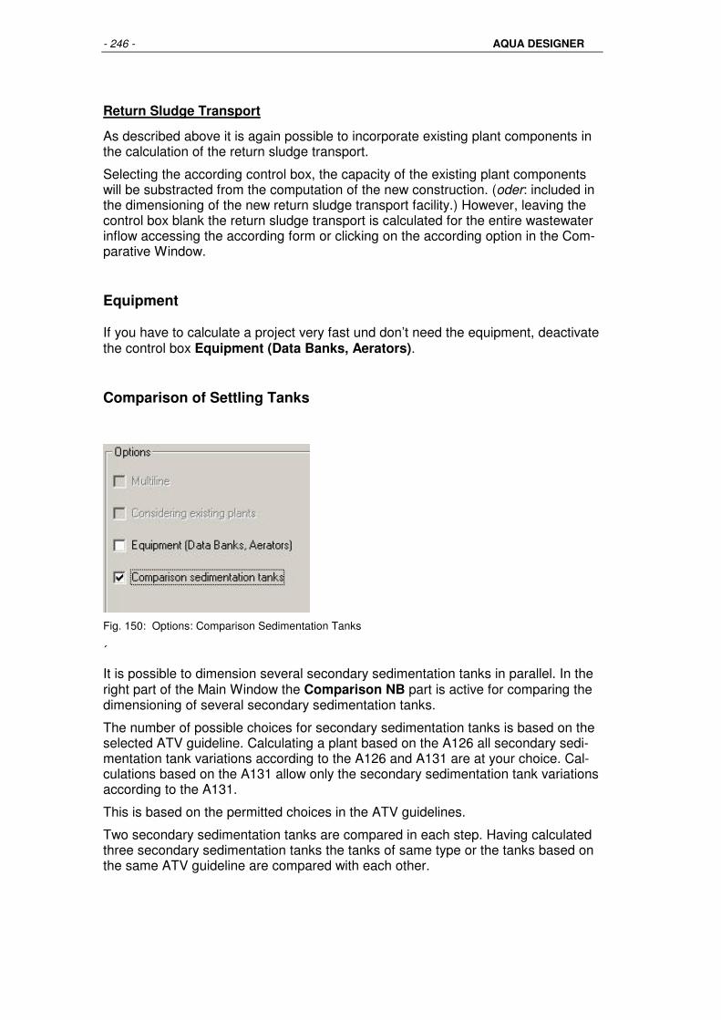
- 246 - AQUA DESIGNER
Return Sludge Transport
As described above it is again possible to incorporate existing plant components in the calculation of the return sludge transport.
Selecting the according control box, the capacity of the existing plant components will be substracted from the computation of the new construction. (oder: included in the dimensioning of the new return sludge transport facility.) However, leaving the control box blank the return sludge transport is calculated for the entire wastewater inflow accessing the according form or clicking on the according option in the Com-parative Window.
Equipment
If you have to calculate a project very fast und don’t need the equipment, deactivate the control box Equipment (Data Banks, Aerators).
Comparison of Settling Tanks
Fig. 150: Options: Comparison Sedimentation Tanks
´
It is possible to dimension several secondary sedimentation tanks in parallel. In the right part of the Main Window the Comparison NB part is active for comparing the dimensioning of several secondary sedimentation tanks.
The number of possible choices for secondary sedimentation tanks is based on the selected ATV guideline. Calculating a plant based on the A126 all secondary sedi-mentation tank variations according to the A126 and A131 are at your choice. Cal-culations based on the A131 allow only the secondary sedimentation tank variations according to the A131.
This is based on the permitted choices in the ATV guidelines.
Two secondary sedimentation tanks are compared in each step. Having calculated three secondary sedimentation tanks the tanks of same type or the tanks based on the same ATV guideline are compared with each other.

Menu Options - 247 -
Fig. 151: Comparison of Secondary Sedimentation Tanks
Example: Calculate the vertical-flow secondary sedimentation tank based on the ATV A126 and ATV A131. In the right part of the Main Window the field Comparison NB with the field vertical A126/A131 is activated. Additionally calculate the horizontal-flow secondary sedimentation tank based on the A126. Now the fields A126 horizontal/vertical and vertical A126/A131 are activated.
Clicking on any active field opens a window that compares selected values of the secondary sedimentation tanks. Select one of the computed secondary sedimenta-tion tanks by clicking on the according option field.
Without an individual selection at this time the very first computed secondary sedi-mentation tank is preselected by the program.
Leave the window by clicking on OK.
The dimensions of the selected tank are used for the subsequent computation.
Example: Calculate the vertical-flow secondary sedimentation tank based on the ATV A126 and ATV A131. In the right part of the Main Window the field Comparison NB with the field vertical A126/A131 becomes activ. Additionally calculate the horizontal-flow secondary sedimentation tank based on the A126. Now the fields A126 horizontal/vertical and vertical A126/A131 are activ.
Clicking on an activ field opens a window with comparative values for the secondary sedimentation tanks. Choosing an option field one of the computed secondary sedi-mentation tanks is selected.
Without an individual selection the very first computed secondary sedimentation tank is preselected by the program.
Leave the window clicking on OK.
The values of the selected tank are used for the subsequent computation.

- 248 - AQUA DESIGNER
Documentation
If you chose these items they will appear in the documentation.
Fig. 152: Options > Settings > Documentation
Operation Costs
As in Documentation, some items can be selected.
Fig. 153: Options > Settings > Operation Costs
Export to Word
All Documentation can be exported to Word. If the Formular Editor is not installed, instead of the formulas an Error will appear. In the chineses language version this also can occur if you work with an chineses operation system.
If its not possible to solve this problem in Word, you are able to change the export conditions for formulas.
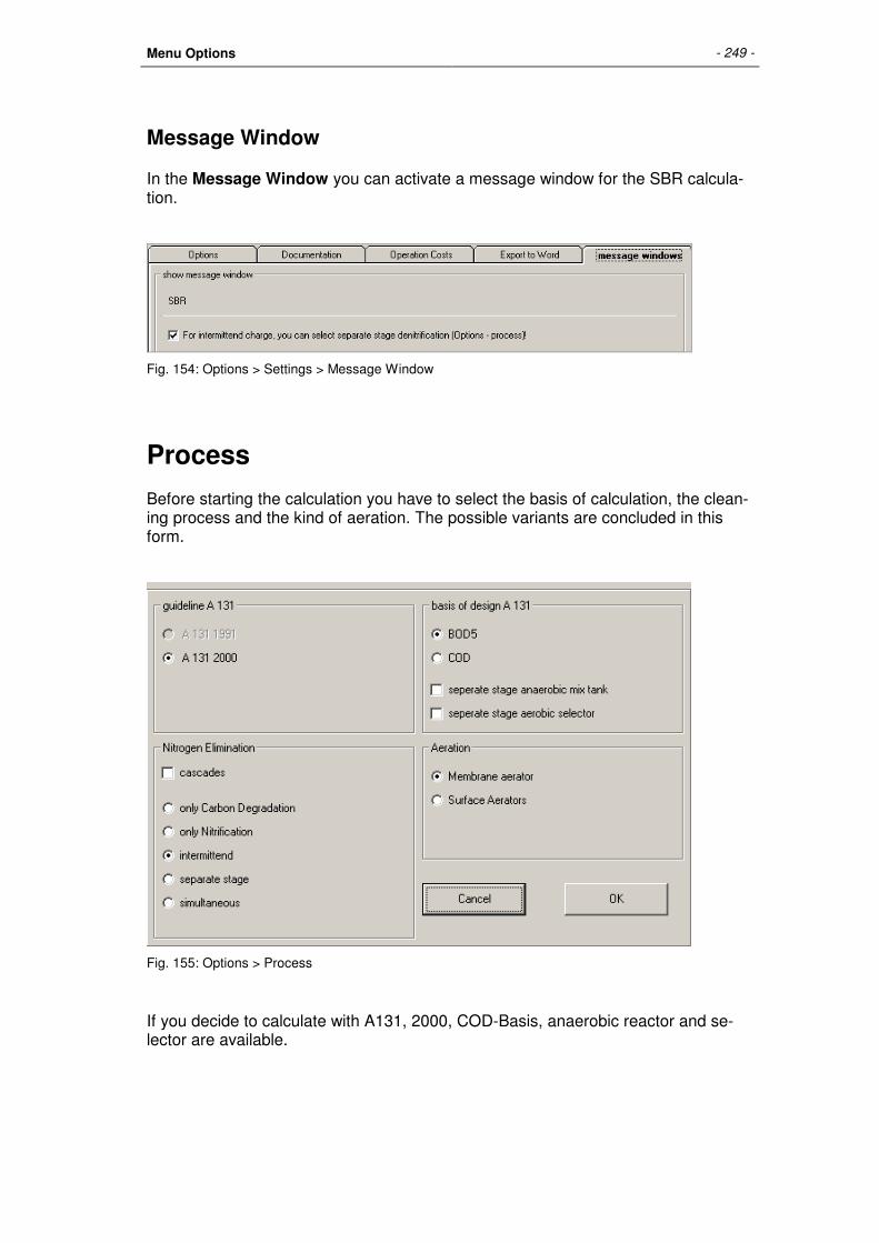
Menu Options - 249 -
Message Window
In the Message Window you can activate a message window for the SBR calcula-tion.
Fig. 154: Options > Settings > Message Window
Process
Before starting the calculation you have to select the basis of calculation, the clean-ing process and the kind of aeration. The possible variants are concluded in this form.
Fig. 155: Options > Process
If you decide to calculate with A131, 2000, COD-Basis, anaerobic reactor and se-lector are available.

- 250 - AQUA DESIGNER
General Constants
Generell
Fig. 156: Options > Generell Constants: Generell
When calculating the sludge load, the temperature is taken into account based on a selected sludge age and in accordance with the ATV A131. For climate conditions very different from those in western Europe it is necessary to change the tempera-ture. For example an average temperature of 20 or 25 °C should be selected for (most) african countries.
Nitrogen Balance
N-Incorporation in the biomass
The preselected value for the fraction of microorganisms nitrogen incorporation is a recommended value from the ATV guideline. For special or extraordinary composi-tions and differing ratios of the BOD5 and nutrients in the wastewater, it is neces-sary to determine the composition and select suitable values in the program.
Fig. 157: Options > Process: Nitrogen Balance

Menu Options - 251 -
Sludge Treatment
Fig. 158: Options > Generell Constants: Sludge Treatment
The MLSS of several sludge treatment steps are based on experience. In AQUA DESIGNER everytime you get recommended values, based on literature. The dry solids concentration depends on the kind of thickening or dewatering process. For example in a filter belt you get a different concentration than in a filter press or a decanter.
Therefore it is able to edit these values and to enter your own MLSS concentration for each step.
The chosen dry solids concentrations also have influence on the supernatant amount.
Fig. 159: Steps of Sludge Treatment

- 252 - AQUA DESIGNER
Buildings / Equipment
Choose Options > Generell Constants > Building / Equipment. Enter your data for building, machines, aeration and flow velocity.
Fig. 160: Options > Generell Constants: Buildings / Equipment
Precipitant
Click on Options > Generell Constants > Precipitant.
Here you can enter new precipitants and choose other parameters for the external C-Dosage. On the left site you could vary some parameters of iron and aluminium salt.
Fig. 161: Options > Generell Constants: Precipitant

Menu Options - 253 -
Constants COD
Click on Options > Constants COD. In the formular you set the arguments for the Chemical oxygen demand COD.
Fig. 162: Options > Constants COD
Constants Hochschulgruppe
Choose Options > Constants Hochschulgruppe. In this formular you can vary a lot of parameters, like kinetic, stöchiometric or oscillation factors.
Fig. 163: Options > Constants Hochschulgruppe

- 254 - AQUA DESIGNER
Details
Shock Factors for Oxygen Supply
The ATV guideline is not universely accepted and employed in all its details in Ger-man counties. This particularly affects the dimensioning of aeration systems. The program can adapt to different values for carbondioxide and nitrogen respiration. However, the ATV values offer a safe alternative for dimensioning the oxygen sup-ply.
Immersion Depth
The difference between water depth and immersion depth depends on the construc-tion of the aeration system. A distance of 30 cm is applicable for most of the sys-tems. You may enter another value for other construction plans. For example, in case of pressure loss at a limit for blowers you may enter a lower difference to in-crease the immersion depth.(Changing the immersion depth makes it possible to achieve a lower or higher pressure for the blowers.)
Pressure Losses in the Air Pipes
The pressure loss in the air pipes are automatically added to the immersion depth for dimensioning of the blowers. This pressure loss depends on the total length of the pipes, the pipe layout, and to a large extent on the selected aeration equipment and aerator load. The preselected value has been proven to be sufficient in prac-tice. However, you can change this factor when you are sure about a lower pressure loss of your system and thus, the system will work more economically lowering op-erating costs.
SSRS / SSBS
The ratio of the mixed liqour suspended solids concentration at the bottem of the sedimentation tank and in the return sludge is dependent on the selected sludge removal system.
A ratio of 0.5 is suggested for a suction remover. A value of 0.7 should ideally be selected for a sludge scraper. The ratio will automatically be selected as 1 for the hopper-bottomed secondary sedimentation tank as there is no special removal sys-tem required.
Water Level Difference
The water level difference of the activated chamber and the sedimentation chamber results from a hydraulic calculation. The hydraulic calculation is not yet part of

Menu Options - 255 -
AQUA DESIGNER. An average value 10 – 30 cm is suggested. The lower value is in effect for compact systems, the higher value for separate chambers.
Sedimentation Tank Wall Thickness
For a compact system, the thickness of the sedimentation tank wall is taken into account when calculating the activated sludge tank outer diameter and volume.
It is not possible to change this value in the form drawings. For changing the wall thickness value, it is necessary to recalculate the activated chamber starting from the sedimentation tank step.
Bottom Slope /Circular Chambers
For the bottom slope of the sedimentation chamber the commonly applied value of 1/15 or 3.8° is preselected.
Enter a slope of 0° when using a suction remover and remember then to change the MLSS ratio. This is not automatically done by the program as the factor of 0.5 is not explicitly required.
Bottom Slope / Rectangular Chambers
A lower angle for the slope can be selected for a rectangular chamber. In AQUA DESIGNER, like the value for circular chambers, the default value is set as 1/15 or 3,8°.
Cone Base Diameter
A cone is present in several constructions for sedimentation tanks. For compact chambers the basic diameter is the diameter at the bottom of the tank. This value will be taken into account for calculating the hopper-bottom tank water depth.
For sedimentation tanks with flat bottoms, the basic diameter is the diameter at the bottom of the sludge collecting cone.
Flow Velocities
The diameter of air and water pipe lines is calculated using the flow velocity of water and air. For more information see the chapter Extras > Pipe Lines.

Formulaic Symbols - 256 -
FORMULAIC SYMBOLS
German English Unit Description
a A Respiration growth factor ADüker Asyphon m² Surface of the inlet in sedimentation chambers ANB AST m² Surface of the Sedimenation Chamber
Al Al mg/l Precipitant amount in Aluminium
αOC α Quotient of oxygen transfer in activated sludge and in clean water
B B Part of nutrient in biomass (xH+xA), Hochschu-lansatz
bA bA d-1 die rates of autotrophic organism, Hochschulan-satz
bH bH d-1 Die rates of heterotrophic organism, Hoschu-lansatz
BB AT Activated Chamber/ Aeration Tank BBelüfter BAerator m³/(m*h) Load of the Aerators Bd,BSB5 Bd,BOD5
F/M* kg/d BOD5-Charge
BR BR,BOD5 kg/(m³*d) BOD5-volume loading BSB5 BOD5 mg/l Biological oxygen demand in 5 days BSB5zu BOD5i mg/l Inflow concentration to the activated chamber BTS BSS,BOD kg/(kg*d) BOD5-sludge loading C C l/m³ Suldge concentration depending on the thickening
time in the sedimentation chamber ci/g ci/g mg/l Concentration of industriell or trade waste water
components cp Cp kJ/(kg*K) specific heat capacity Cs Cs mg/l Dissolved oxygen saturation concentration de-
pendent on the temperature and partial pressure Cs,theor Cs,theor mg/l Oxygen Saturation Concentration at an average
temperature CSB COD mg/l Chemical oxygen demand Cx Cx mg/l Desired dissolved oxygen concentration in aeration
tanks (DO) DBB DAT m Outer free diameter of the activated chamber DBBSohle DAT,Bottom m Diameter of the sedimentation chamber at the bot-
tom of the activated chamber (compact plant) DDüker Dsyphon m Diameter of the inlet fo sedimentation chambers DNB DST m Diameter of the sedimentation chamber Dspitze Dbottom m Diameter of hopper tanks at the bottom dT dT K Increasment of temperature DTrichter Dhopper m Diameter of the sludge collecting cone in horicontal
floaded sedimentation chambers E I I Inhabitants

Formulaic Symbols - 257 -
ε ε Part of heat emission of the motor power E E kWh/a Yearly energy demand for wastewater transport Eh Eh kWh/h Hourly energy demand for wastewater transport EW PT - Total number of inhabitants and population equiva-
lents referred to the parameters BOD or COD fA fA Volume exchange ratio fA,max fA,max Maximum volume exchange ratio fA,vor fA,vor Proposed volume exchange ratio fA,TW fA,TW Volume exchange ratio at dry weather fC fC - Peak factor for carbon respiration fN fN - Peak factor for ammonium respiration fO2 fO2 gO2/(m³*
m) Oxygen transfer capacity
Fe Fe mg/l Precipitant amount in Fe FS FS m Flow distance in the sedimentation chamber ftbh ftbh - Conversion factor for temperature influent G G m/s² Gravitation factor Ga Ga Dollar/a Yearly salary for one person f' F' Safety factor FD FD Decreasing of respiration at anoxic conditions Fi Fi Inert part out of biomass degradation fT,A fT,A Temperature factor for autotrophic growth fT,bA fT,bA Temperature factor for the autotrophic die rate fT,bH fT,bH Temperature factor for the heterotrophic die Fp Fp Part of inert solids
η η Yield of BOD-degradation
H H M Manometric transportation height (pumping head) h1 h1 M Height of the clear water zone in the sedimentation
chamber h2 h2 M Height of the dividing zone in the sedimentation
chamber h3 h3 m Height of the storage zone in the sedimentation
chamber h4 h4 m Height of the thickening zone in the sedimentation
chamber HBB HAT m Water depth of the activated Chamber he He m Infiltration height of the inlet hE HE m Immersion depth of air hges hges m Water depth in the sedimentation chamber HKegel HCone m Difference between the peripheral water depth and
the depth at the sludge collecting cone in the sedi-mentation chamber
HMitte Hmiddle m Water depth at the sludge collecting cone in the sedimentation chamber
hmittel haverage h/d Hour index hNB hST m Water depth in the sedimentation chamber

- 258 - AQUA DESIGNER
HNBRand HNBper m Peripheral water depth in the sedimentation cham-ber
hs Sludge level ht Ht m Cone height of a hopper tank hw Hw m Water level hz Hz m Cylindrical height of a hopper tank ISV ISV ml/g Sludge volume index iB IB Part of Nutrient in the Biomass iI iI Part of Nutrient in the inert mass ip ip Part of phosphate in the biomas kLa kLa - Aeration factor at temperature T KN Half-life constant for Nmax LBelüfter LAerator m Aerator length MAl Mal g/mol Atom mass Aluminium MFe MFe g/mol Atom mass Iron MP MP g/mol Atom mass Phosphorus mz Number of cycles n N Rainwater factor Nab Ne kg/d Nutrient in the effluent NB NB Sedimentation Chamber Nbio Nbio mg/l Inkorporated nutrient Nd,m1 e denitrificable nutrient Nd,m2 Nutrient to be denitrificated Neigung Slope Slope of the bottom at horizontal floaded sedimen-
tation tanks nG nG Number of blowers NDeni kg/d Denitrificated nutrient NH4-Ne,Sp
mg/l Peak ammonia outlet nitrification
NH4-Ne,m
mg/l Middle ammonia outlet concentration
Nn,Sp mg/l Nitrificable peak ammonia inlet Nn,m mg/l Averabge nitrificable ammonia inlet Nanorg mg/l Anorganic nutrient concentration outlet Norg mg/l Organic nutrient concentration outlet NO3-N NO3-N mg/l Nitrate-N NO3-ND NO3-ND mg/l Denitrificated Nitrate-N-Concentration NO3-Ne NO3-Ne mg/l Nitratd-N in the effluent NNitri kg/d Nitrificated nutrient nR nR Rain frequency NÜS Nutrient in waste sludge Nzu Nzu mg/l Nutrient-N-Concentration in the inflow nmax,A Maximum growth rate, OB OB kg/kg Oxygen charge OBmittel OBaverage kg/kg Oxygen charge without stress factors OC Oxygen transfer capacity

Formulaic Symbols - 259 -
OCA Minimum oxygen input for surface aeration OP Oxygen efficiency OV Oxygen consumption OVC OVC kg/kg Specific oxygen demand for BOD5-degradation
OVN OVN kg/kg Specific oxygen demand for the oxidation of
nutrient, related to BOD5 Po Phosphate concentration inlet Pe Phophate concentration outlet P mg/l Orthophosphate concentration Pa Pa DM/a Yearly staff costs Pelim kg/d Phospate for removal Pn Pn - Number of persons qA qA m/h Surface loading Qf Qf m³/h Inflow of extraneous water per hour Qfd Qfd m³/d Inflow of extraneous water per day Qg Qg m³/h Inflow of trade wastewater per hour Qgd Qgd m³/d Inflow of trade wastewater per day Qh Qh m³/h Inflow of domestic wastewater per hour Qi Qi m³/h Inflow of industriell wastewater per hour Qid Qid m³/d Inflow of industriell wastewater per day QL QL m³/h Air volume flow per hour QLGebläse QLBlower m³/h Capacity of a blower QLBetrieb QLBetrieb m³/d Daily air demand in operation Qm Qm m³/h Stormwater inflow Qmittel Qaverage m³/h Average hourly inflow QR QRS
Qr* m³/h Return sludge flow
Qs Qs m³/h Inflow of wastewater per hour Qsd Qsd m³/d Inflow of wastewater per day qsv qsv l/(m²*h) Sludge volume loading QSp Inflow according to nitrificabel nutrient concentra-
tion Q24 24-hours average Qt Qt m³/h Inflow at dry weather per hour Qtd Qtd m³/d Inflow at dry weather per day Qzu Qzu m³/d Inflow of Wastewater per day ρ ρ kg/m³ Density ρL ρL kg/m³ Density of air RS RS - Return Sludge RV RV - Return sludge relation RZ Recirculation ratio RZges Recirculation ratio including return sludge rx Part of returned nutrient out of waste sludge ß ß - Molar relations for precipitants in the phosphate
elimination

- 260 - AQUA DESIGNER
S T °C Wastewater temperature So' td h/d Daily working time of 1 person SKe Alkalinity outlet SKo Alkalinity inlet T Temperature td Daily working time
tE tE h Thickening time for TSBS (MLSS) at the Bottom of
the sedimentation tank TKN TKN mg/l Kjeldahl-nutrient-concentration (Ammonia-N and
organic N) tL tL h/d Operation time of the blowers tLdim tLdim h/d Aeration time out of the dimensioning tS Storage time TSBB TSBB
MLSS* kg/m3 Mixed liqour suspended solids in the activated
chamber
TSBS TSBS kg/m³ Concentration of TS (MLSS) at the bottom of the sedimentation tank
TSo TSo mg/l TS in the inflow of the activated chamber TSR TSR kg/m³ TS in the reactor (here the activated chamber) TSRS TSRS
XR* kg/m³ Solids concentration in the return line
TSR,TW tTS tTS
θc* d Sludge age, cell residence time
tTS,A d Aerobic sludge age tTS,G d Total sludge age tZ Time of cycle tR Time of reaction tD Time of denitrification tN Time of nitrification θH Hydraulical retention time in an activated sludge
system ÜS ÜS
Px* Excess sludge
* /17/ Hochschulansatz ÜSB ÜSB
kg/kg Specific excess sludge production related to BOD5
ÜSBSB5 ÜSBOD5 kg/kg Part of the biological excess sludge production ÜSp ÜSp kg/kg Part of the chemical excess sludge production V1 V1 m³ Volume of the clearwater zone V2 V2 m³ Volume of the dividing zone V3 V3 m³ Volume of the storage zone V4 V4 m³ Volume of the thickening zone VBB VBB m³ Volume of the activated chamber VD Denitrification volume VN Nitrification volume VR VR m³ Volume of the reactor

Formulaic Symbols - 261 -
VR,TW Volume at dry weather Vmin VBBmin m³ Minimum volume of the activated chamber ∆V Exchange volume ∆VTW Exchange volume at dry weather VSV Sludge volume (by the dilution method) vs Settling volocity
VU VU m³ Volume of the sedimentation chamber under the
bottom of the activated chamber at compact plants VÜS Volume of waste sludge ws Water usage from A126, A131 x h/d hour index from A118 xA Part of autotrophic organism in activated sludge xH Part of heterotrophic organism in activated sludge xI Inert part in activated sludge xF Precipitation sludge in activated sludge YH Yield of heterotrophic biomass YA Yield of autotrophic biomass

- 262 - AQUA DESIGNER
LITERATURE
/1/ Härtel, Lutz (1990): Modellansätze zur dynamischen Simulation des Belebtschlammverfahrens WAR Schriftenreihe, Darmstadt, Nr. 47
/2/ ATV Arbeitsblatt A 131, (1991): Bemessung von einstufigen Belebungsanlagen ab 5000 Einwohnerwerten Gesellschaft zur Förderung der Abwassertechnik e.V. (GfA), Hennef
/3/ ATV Arbeitsblatt A 126, (1993): Grundsätze für die Abwasserbehandlung in Kläranlagen nach dem Bele-bungsverfahren mit gemeinsamer Schlammstabilisierung bei Anschlußwerten zwischen 500 und 5000 Einwohnerwerten Gesellschaft zur Förderung der Abwassertechnik e.V. (GfA), Hennef
/4/ ATV Arbeitsblatt A 202, (1992): Verfahren zur Elimination von Phosphor aus Abwasser Gesellschaft zur Förderung der Abwassertechnik e.V. (GfA), Hennef
/5/ Boll, Dr. Ing. R.: Kläranlagen ab 5000 EW (A 131, AB 2.5/2.6, 2/93) ATV-Regelwerkskurs Abwasserreinigung 27. - 29.11.95 in Weimar
/6/ ATV Arbeitsblatt A 203, (1995): Abwasserfiltration durch Raumfilter nach biologischer Reinigung (GfA), Hennef
/7/ ATV-Arbeitsberichte: Anwendungshinweise zum ATV Arbeitsblatt A 131-Teil Nachklärbecken Korrespondenz Abwasser 2/93
/8/ Arbeitsbericht des ATV-Fachausschusses 2.12 „Betrieb von Kläranlagen“ Personalbedarf für den Betrieb von Kläranlagen Korrespondenz Abwasser, 6/94
/9/ Heinz Patt, Andreas Stein: Einsatz belüfteter Sandfänge auf Kläranlagen Korrespondenz Abwasser 9/96
/10/ Norbert Meyer: Biologische Phosphatelimination und simultane Denitrifikation Abwassertechnik 4/94, Bauverlag GmbH, Wiesbaden
/11/ von der Emde, Univ.-Prof. Dr.-Ing Wilhelm: Achtzig Jahre Belebungsverfahren KA-Betriebs-Info, Hennef, 4/95
/12/ Rheinheimer G., Hebemann W., Raff J. Sekoulov I.: Stickstoffkreislauf im Wasser R. Oldenbourg-Verlag, München-Wien, 1988
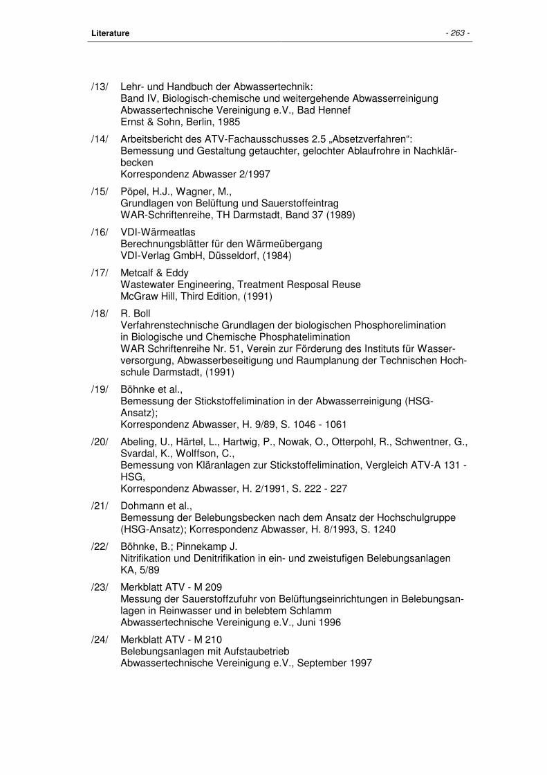
Literature - 263 -
/13/ Lehr- und Handbuch der Abwassertechnik: Band IV, Biologisch-chemische und weitergehende Abwasserreinigung Abwassertechnische Vereinigung e.V., Bad Hennef Ernst & Sohn, Berlin, 1985
/14/ Arbeitsbericht des ATV-Fachausschusses 2.5 „Absetzverfahren“: Bemessung und Gestaltung getauchter, gelochter Ablaufrohre in Nachklär-becken Korrespondenz Abwasser 2/1997
/15/ Pöpel, H.J., Wagner, M., Grundlagen von Belüftung und Sauerstoffeintrag WAR-Schriftenreihe, TH Darmstadt, Band 37 (1989)
/16/ VDI-Wärmeatlas Berechnungsblätter für den Wärmeübergang VDI-Verlag GmbH, Düsseldorf, (1984)
/17/ Metcalf & Eddy Wastewater Engineering, Treatment Resposal Reuse McGraw Hill, Third Edition, (1991)
/18/ R. Boll Verfahrenstechnische Grundlagen der biologischen Phosphorelimination in Biologische und Chemische Phosphatelimination WAR Schriftenreihe Nr. 51, Verein zur Förderung des Instituts für Wasser-versorgung, Abwasserbeseitigung und Raumplanung der Technischen Hoch-schule Darmstadt, (1991)
/19/ Böhnke et al., Bemessung der Stickstoffelimination in der Abwasserreinigung (HSG-Ansatz); Korrespondenz Abwasser, H. 9/89, S. 1046 - 1061
/20/ Abeling, U., Härtel, L., Hartwig, P., Nowak, O., Otterpohl, R., Schwentner, G., Svardal, K., Wolffson, C., Bemessung von Kläranlagen zur Stickstoffelimination, Vergleich ATV-A 131 - HSG, Korrespondenz Abwasser, H. 2/1991, S. 222 - 227
/21/ Dohmann et al., Bemessung der Belebungsbecken nach dem Ansatz der Hochschulgruppe (HSG-Ansatz); Korrespondenz Abwasser, H. 8/1993, S. 1240
/22/ Böhnke, B.; Pinnekamp J. Nitrifikation und Denitrifikation in ein- und zweistufigen Belebungsanlagen KA, 5/89
/23/ Merkblatt ATV - M 209 Messung der Sauerstoffzufuhr von Belüftungseinrichtungen in Belebungsan-lagen in Reinwasser und in belebtem Schlamm Abwassertechnische Vereinigung e.V., Juni 1996
/24/ Merkblatt ATV - M 210 Belebungsanlagen mit Aufstaubetrieb Abwassertechnische Vereinigung e.V., September 1997

- 264 - AQUA DESIGNER
/25/ Konrad Stania, Manfred Lehner, Raimund Haberl Denitrifikation in intermittierend betriebenen Belebungsanlagen (SBR) Korrespondenz Abwasser, 1/97, S. 61 – 65
/26/ 4. Abwasser-Tagung SBR-Technik - Anlagenbauer und Planer berichten über ihre Erfahrungen in Deutschland Verband Deutscher Maschinen- und Anlagenbauer e.V., 11/97
/27/ Bever, Stein, Teichmann Weitergehende Abwasserreinigung Oldenbourg-Verlag, 2.Auflage
/28/ Dr.-Ing. Martin Wagner Sauerstoffeintrag und Sauerstoffertrag von Belüftungssystemen und deren Bestimmung mit modernen Messmethoden Schriftenreihe WAR des Instituts WAR der TU Darmstadt, Darmstadt 1997
/29/ H.J. Pöpel Grundlagen der chemischen Phosphorelimination WAR Schriftenreihe Nr. 51, Verein zur Förderung des Instituts für Wasser-versorgung, Abwasserbeseitigung und Raumplanung der Technischen Hoch-schule Darmstadt, (1991)
/30/ Arbeitsbericht der ATV-Arbeitsgruppe 2.6.6 “Biologische Phosphorentfer-nung” Korrespondenz Abwasser 3/89
/31/ Arbeitsbericht der ATV-Arbeitsgruppe 2.6.1 Blähschlamm, Schwimmschlamm und Schaum in Belebungsanlagen – Ursachen und Bekämpfung Korrespondenz Abwasser 10/98
/32/ ATV-Handbuch Mechanische Abwassereinigung Abwassertechnische Vereinigung e.V., Bad Hennef Ernst & Sohn, Berlin, 1996
/33/ M. Boes, Anordnung und Bemessung der Luftzufuhr von belüfteten Sandfängen Korrespondenz Abwasser 7/90
/34/ A. Stein Ein Beitrag zur Gestaltung belüfteter Sandfänge Korrespondenz Abwasser 4/92
/35/ J. Londong Beitrag zur Bemessung belüfteter Sandfänge Korrespondenz Abwasser 1/88
/36/ ATV-Arbeitsbericht der ATV-Arbeitsgruppe 2.5.1 "Sandfänge" im ATV-Fachausschuß 2.5 Absetzverfahren Sandabscheideanlgen (Sandfänge und Sandfanggutaufberreitungsanlagen) Korrespondenz Abwasser 3/98
/37/ Kalbskopf, K.H.: Die Bemessung von Sandfängen unter Berücksichtigung der Strömungstur-bulenzen; Kommunalwirtschft 1966, Heft 9

Literature - 265 -
/38/ Martin Wagner, Peter Cornel, Stefan Krause (Darmstadt) Sauerstoffeintrag und α-Werte in Membranbelebungsanlagen Korrespondenz Abwasser 11/2001
/39/ ATV-DVWK Arbeitsblatt A 131, (2000): Bemessung von einstufigen Belebungsanlagen Gesellschaft zur Förderung der Abwassertechnik e.V. (GfA), Hennef
/40/ Thomas Werner Beitrag zur Bemessung von einstufigen Belebungsanlagen mit Kaskadende-nitrifikation Berichte zur Siedlungswasserwirtschaft, Nr. 9 TU Berlin, FG Siedlungswasserwirtschaft, 1998
/41/ N. Jardin Rückläufe aus der Schlammbehandlung – Menge, Beschaffenheit und Aus-wirkungen WAR Schriftenreihe Nr. 66, Verein zur Förderung des Instituts für Wasser-versorgung, Abwasserbeseitigung und Raumplanung der Technischen Hoch-schule Darmstadt, (1993)
/42/ ATV Arbeitsbericht 3.2 Maschinelle Schlammentwässerung Korrespondenz Abwasser 2/1995
/43/ Fachausschuss KA-5 „Absetzverfahren“ Vorklärbecken in modernen Kläranlagen Korrespondenz Abwasser 8/2003
/44/ Karl und Klaus R. Imhoff Taschenbuch der Stadtentwässerung 29. Auflage, 1999 R. Oldenbourg Verlag München Wien
/45/ Rolf Kayser ATV-DVWK-Kommentar zum ATV-DVWK-Regelwerk Bemessung von Belebungs- und SBR-Anlagen Deutsche Vereinigung für Wasserwirtschaft, Abwasser und Abfall e.V. Hen-nef, 2001
/46/ Merkblatt ATV-DVWK-M 363 Herkunft, Aufbereitung und Verwertung von Biogasen Deutsche Vereinigung für Wasserwirtschaft, Abwasser und Abfall e.V. Hen-nef, 8/2002
/47/ Merkblatt ATV-DVWK-M 368 Biologische Stabilisierung von Klärschlämmen Deutsche Vereinigung für Wasserwirtschaft, Abwasser und Abfall e.V. Hen-nef, 4/2003
/48/ Rolf Otte Witte Rückbelastung der Kläranlage aus der Schlammbehandlung ATV-Handbuch Klärschlamm 4. Auflage Ernst & Sohn, Berlin, 1996
/49/ Bischofsberger, Dichtl, Rosenwinkel, Seyfried, Böhnke Anaerobtechnik 2. Auflage, Springer Verlag, 2005
- 266 - AQUA DESIGNER
/50/ Henz, Harremoës, la Cour Jansen, Arvin Wastewater Treatment Biological and Chemical Processes Third Edition, Springer Verlag, 2002
/51/ N.F. Gray, Biology of Wastewater Treatment, 2nd Edition 2004, Imperal College Press
/52/ C.W. Randall, J.L. Barnard, H.D. STensel, Water Quality Maanagement Li-brary Volume 5: Design and Retrofit of Wastewater Treatment Plats for Biological Nutrient Removal Technomic Publishing, 1992
/53/ Valerie Naidoo, Municipal Wastewater Characterization Dissertation 1999, University of Nata, Durban
/54/ Aarne Vesilind, Wastewater Treatment Plant Design, Water Environment Federation, IWA Publishing, 2004
/55/ N.F.Gray: Biology of Wastewater Treatment; 2nd Edition 2004; Imperial Col-lege Press
/56/ Metcalf & Eddy: Wastewater Engineering - Treatment Disposal Reuse; 3rd Edition 1991; McGraw-Hill
/57/ Merkblatt ATV-DVWK-M 198 Vereinheitlichung und Herleitung von Bemessungswerten für Abwasseranla-gen, Deutsche Vereinigung für Wasserwirtschaft, Abwasser und Abfall e.V. Hennef, 4/2003

Literature - 267 -
Index
Aanaerobic tank ............................. 39
Activated chamber
separate.................................... 137
Activated sludge plant .................... 89
Activated sludge process
theory.......................................... 34
Activated sludge tank ................... 131
activated chamber....................... 25
minimum diameter .................... 135
real sludge age ......................... 140
tank proportions .......................... 25
true volume ............................... 136
verification................................. 139
Actual volume................................. 87
Aerated grit chamber.................... 199
Aeration.......................................... 26
dimensioning temperature......... 146
loading condition ....................... 147
Aeration lattice
construction .............................. 156
header pipes ............................. 153
Aeration lattices............................ 153
Aeration period............................... 91
Aerator disc.................................. 153
Aerator load ................................. 155
Aerobic selector ........................... 110
Aerobic Sludge Stabilization
Aerob Thermophile ................... 217
Air Demand............................... 217
Environmental Temperature...... 216
Key Data ................................... 216
Aerobic Sludge Treatment
Environmental Temperature...... 213
Handling.................................... 214
Sludge Thickening .................... 214
Air consumption ........................... 141
Air volume
hourly ........................................ 151
AlCl3 ............................................... 40
Aluminium................................. 82, 94
Aluminium chloride ......................... 94
Ammonia ........................................ 37
Ammonia nitrogen in effluent .......... 89
Ammonification............................... 37
Anaerobic phase............................. 39
Anaerobic stabilization of sludge .. 209
Ardern ............................................ 34
Atomic masses ............................... 95
ATV A118....................................... 45
ATV A126 guideline........ 54, 114, 117
ATV A131 guideline................ 54, 117
ATV A202....................................... 94
ATV guidelines ............................... 53
ATV worksheets ............................. 33
ATV-Committee 2.12 .................... 204
ATV-Fachausschuss 2.12............. 204
Autotrophic bacteria........................ 38
Basic data ............................... 22, 81
Belastung
Abwasserzufluß........................... 45
Biodegradation ............................... 36
Biological association ..................... 36
Biological excess sludge production85
Biologically active micro-organisms 35
Biologically removed phosphorus ... 94
Blower .......................................... 151
room temperature...................... 194
BOD5 ............................................. 47
BOD5-sludge load........................... 36
Bouyancy...................................... 233
Buffer capacity................................ 38
Cascaded denitrification ................. 62

- 268 - AQUA DESIGNER
Centrifugal fan ..............................158
Chemical precipitation.....................40
Clarified water outlet .....................129
Clear water zone...................120, 124
Combined heat and power unit .....209
Compact plant ..............................134
scaled drawing...........................136
Comparative window.....................114
Comparing sedimentation tanks ...246
Completed dimensioning ................42
Component selection ....................196
Compressor ..................................190
Conformity ......................................87
Control box .....................................15
Control graph..........................26, 136
Conventions......................................9
Counter pressure..........................189
Cycle period..................................164
Databank ................................26, 185
air lift pump................................190
blower..................................26, 189
further data................................186
mixer .........................................188
mixing devices ...........................188
new data....................................186
new key .....................................186
pumps .......................................187
save data...................................186
search key.................................186
transport capacity ......................187
Deep secondary sedimentation.....134
Denitrification......................81, 89, 91
cascaded.....................................62
Denitrification process ..................142
Description..............................31, 192
Design temperature ........................89
Detention time ................................35
Diameter ...................................... 116
Dimensioning ............................31, 33
Dimensioning temperature ........... 146
denitrification capacity................. 60
increased .................................... 60
Disc aerator
diameter.................................... 155
load........................................... 155
Disposal costs.............................. 204
Disposal of grit and grease .......... 203
Disposal of screenings ................. 203
Double-sided overflow weir .......... 131
Drawing...................................31, 225
aeration system ........................ 230
export........................................ 231
print........................................... 231
Energy consumption .................... 148
Energy input................................. 157
English ........................................... 33
Enhanced biological uptake ........... 39
Equation for the denitrification........ 38
Eutrophic waters ............................ 38
Excess sludge...........................36, 95
production ............84, 85, 102, 104
volume ...................................... 204
Extension ....................................... 29
Extern-C-dosage
calculation................................... 71
carbon sources ........................... 68
infliction....................................... 68
milieu .......................................... 69
organic partl ................................ 76
pH............................................... 70
precipitent ................................... 74
temperatur .................................. 70
FeCl3 .............................................. 40
Fermenter temperature ................ 212

Literature - 269 -
Filamentous bacteria .................... 110
File name ....................................... 41
Filterable solids .............................. 47
Flocculant..................................... 208
Floor level .................................... 133
Flow distance ............................... 121
Form .............................................. 43
Free boards ................................ 228
Friction rectangle.......................... 234
German.......................................... 33
Gravitational thickening ................ 208
Grease ......................................... 203
separator................................... 199
volume ...................................... 203
Grit
chamber scraper ....................... 199
classifier.................................... 203
classifier opperation period ....... 199
dewatering ................................ 203
transport.................................... 199
Growth rate .............................. 35, 36
Guidelines ...................................... 33
H+-Ion............................................. 38
Header pipes................................ 229
Heat removal................................ 195
Heterotrophic micro-organism .. 36, 38
High loaded peak ......................... 197
Hopper angle ....................... 125, 126
Hopper bottom tank.......113, 114, 125
Horizontal flow secondary sedimentation tank.................... 117
Horizontal flow tanks .................... 114
Hydrolysis....................................... 36
Immersed pipes............................ 129
Immersion depth .......................... 151
Inactive particles .......................... 103
Industrial ........................................ 52
Inflow level ................................... 119
Inlet chamber................................ 119
Inorganic carbon............................. 38
Inorganic polyphosphates............... 39
Input field........................................ 14
Input window................................... 43
Insoluble organic substances ......... 36
Installation ...................................... 10
autorun........................................ 10
by explorer .................................. 10
Intermitted denitrification
cascaded..................................... 64
Intermittent denitrification ............... 33
Invert ............................................ 124
Iron ........................................... 82, 94
Iron(III)-chloride .............................. 94
ISV ................................................. 82
Keyboard function........................... 16
Language ................................. 33, 41
Law of the minimum ....................... 37
Layout
concentrations........................... 194
dry weather flow ........................ 194
scroll bar.................................... 192
title page ................................... 192
Lime conditioning............................ 35
Links............................................... 42
Liquid depth.................................. 120
Liquid level zones ......................... 123
Liquor suspended solids ................. 82
Load ............................................... 44
for organic ................................... 47
industrial...................................... 44
industriell inflow........................... 52
specific ........................................ 47
Loading conditions
aeration ..................................... 147
Lockett............................................ 34
- 270 - AQUA DESIGNER
Main window...................................41
Mass calculation ...........................232
Mechanical thickening.....................35
Membrane aeration...............152, 161
aerator disc................................153
transmembrane pressure difference...............................................162
tubular diffuser...........................153
Menu bar ..................................12, 41
Metabolic turnover ..........................35
Metal mass .....................................95
Minimum diameter ........................117
Minimum heights...........................122
Mixed liquor suspended solids ..83, 84
A126............................................83
Mixing ...........................................157
Mixing devices ..........................33, 91
MLSS..............................................83
influent.........................................84
sludge treatment........................251
Molar ratio.................................94, 96
N2O.................................................38
New project.....................................18
Nitrate-N ........................................89
Nitrification................................89, 91
Nitrobacter ......................................38
Nitrogen..........................................47
deficiency ....................................37
elimination ...................................33
load .............................................89
removal........................................90
Nitrosomonas .................................38
Non vegetation time......................208
Nutrient ratio ...................................37
Operating cost calculation.............196
Operation building.........................192
Operation period...........................199
Operation period of screen ...........199
Option field..................................... 15
Organic load..............................81, 82
Organic load, table A126................ 82
Organic phosphorus....................... 39
Orthophosphate ............................. 39
Outflow......................................... 192
Outlet channels ............................ 130
Outlet pipe ................................... 195
Overflow weirs ............................. 130
Oxidation........................................ 38
Oxidation of ammonia .................. 142
Oxygen charge............................. 142
Oxygen concentration ...........143, 148
Oxygen demand....................141, 150
BSB5-Basic, new ...................... 144
CSB-Basic ................................ 146
specific...................................... 141
Oxygen efficiency......................... 221
Oxygen requirements................38, 91
Oxygen saturation concentration.. 143
Oxygen supply ............................. 149
factor ........................................ 148
hourly........................................ 150
Oxygen transfer ........................... 148
Oxygen transfer capacity
surface aeration ........................ 159
Oxygenation
surface aeration ........................ 158
Package plant .............................. 132
Partial stabilisation ......................... 85
Path name ..................................... 41
P-content ....................................... 39
Personnel costs ........................... 204
Personnel requirement................. 204
Phosphate...................................... 47
aluminium salt ........................95, 96
biological phosphorus removal.... 92

Literature - 271 -
iron salt ................................. 95, 96
precipitation ................................ 96
removal ....................................... 92
Phosphorus.................................... 39
precipitant requirement ............... 95
precipitation ................................ 81
simultaneous precipitation........... 95
Plant efficiency............................. 198
Polyphosphate ............................... 39
Pöpel............................................ 148
Population equivalent ....20, 33, 45, 47
Power consumption........................ 32
Pre sedimentation .......................... 53
retention time .............................. 53
Precipitant application .................... 95
Precipitation sludge...................... 103
Preliminary clarification ................ 199
Preliminary step ............................. 47
Presentation................................... 31
Pretreatment step......................... 192
Primary sedimentation.................... 47
Project name.................................. 20
Pumping stations.......................... 197
Pumps
capacity..................................... 187
centrifugal ................................... 28
power consumption................... 187
pumping head ........................... 187
Pure nitrification ........................... 157
Rain frequency..................... 197, 198
Recirculation ratio ................ 120, 160
A126 ........................................... 88
A131 ........................................... 88
Reduction of nitrate ........................ 38
Reproduction time .......................... 36
Return sludge transportation .... 28, 88
Returned biomass .......................... 35
Rotary piston blower ............. 189, 199
Rotting process ............................ 209
SAE
air demand ................................ 222
membrane aeration ................... 221
mixers ....................................... 224
surface aeration ........................ 223
Safety ............................................. 35
Scraping zone .............................. 120
Screenings
press ......................................... 203
volume....................................... 203
Secondary sedimentation tank ... 21, 246
extern .......................................... 25
variations................................... 114
variations................................... 246
Sedimentation ................................ 35
Selector ........................................ 110
aeration ..................................... 111
design ....................................... 111
mixing........................................ 112
Separate mixing.............................. 26
Separate sewerage system .. 126, 198
Separate stage denitrification
cascaded..................................... 63
Settleability ..................................... 82
Settling zone................................. 120
Sewer system, combined.............. 197
Shock factors................................ 142
Side view ...................................... 231
Single-sided overflow weir ............ 131
Siphon pipe .................................. 195
Slope ............................................ 233
Sludge
age.............................................. 84
buoyancy................................... 121
detention period......................... 208

- 272 - AQUA DESIGNER
detention time..............................29
load .................................36, 82, 84
load, A126 .............................84, 87
Organic Part ..............................216
production....................................36
scraper ......................................121
stabilisation..................................85
tank .....................................29, 207
tank, specific energy..................209
thickening ....................................29
withdrawal pipes ........................121
Sludge treatment ..................206, 207
combined heat and power unit...209
range of application ...................209
Sludge Treatment
Aerob Thermophile ....................217
Aerobic ......................................213
Sludge volume index.................81, 82
Solids concentration in the return sludge........................................120
Specific heat capacity ...................195
Specific operation costs................205
Spur..............................................234
Square grit chamber .....................199
Stability ...........................................35
Stabilizing of sludge
anaerobic...................................209
Staff ................................................32
Standard aeration efficiency .........221
Standard values............................229
Start................................................10
Storage tank .................................197
Storage zone ........................119, 120
Stundensatz ..................................45
Supernatant
concentrations .............................50
loads............................................51
Surface area.................................115
Surface loading rate..................... 115
System requirements ....................... 9
Tank
design ....................................... 125
geometry................................... 131
volume ........................................ 35
Temperature ................................ 146
Thermal efficiency........................ 195
Thickener ..................................... 206
Thickening ................................... 214
Thickening and scraping zone...... 120
Thickening detention period ......... 121
Thickening zone ....................119, 120
Thickening, gravitational .............. 207
Time switch .................................... 39
Title bar.....................................31, 41
TKN................................................ 47
Top view....................................... 231
Total depth................................... 125
Total excess sludge production...... 86
Total sludge production.................. 96
Trade ............................................. 52
Trade load...................................... 81
Transfer of oxygen ....................... 143
Transmembrane pressure difference................................................. 162
True scaled drawings ................... 225
Tubular diffuser .....................150, 153
Unaerated phase ........................... 39
Upflow aerobic selector ................ 110
Urea............................................... 37
Variations of wastewater ................ 35
Verification
sludge load ............................... 140
Vertical flow sedimentation tank.. 113, 115, 126
VN/V-ratio .................................... 105
Volume activated sludge tank

Literature - 273 -
126.............................................. 87
A131 ........................................... 87
Volume flow ................................. 198
Volume loading .............................. 82
Volumetric loading.......................... 84
Wastewater inflow ........................ 194
Water depth.................................. 133
Weir load ...................................... 130
Work space .................................. 232

- 274 - AQUA DESIGNER
SERVICE
BITControl GmbH
Heilenbacherstraße 6
54636 Schleid
Telefon: +49 65 69 / 962 55-11
Telefax: +49 65 69 / 962 55-19
www.bitcontrol.info