B.Sc. Hons. in Software Engineering

CW228

Research Manual

Project Title: Number Plate f

Recognition f

Supervisor: Nigel Whyte __ f

Student ID: C00131013 f

Student Name: Ronghua Ou f

Date: 21 November 2010 f

Table of Contents1. Introduction...............................................................................................................................3

1.1. What is NPR system?.......................................................................................................3

1.2. The process of NPR system.............................................................................................4

2. Existing System..........................................................................................................................6

2.1. Fixed Camera LPR Systems(CDFS)...................................................................................6

2.2. Intertraff Parking Manager..............................................................................................7

2.3. High-definition, multilane ANPR from Watchman...........................................................7

2.4. Conclusion.......................................................................................................................8

3. How to identify a Number Plate................................................................................................9

3.1. Pre-processing.................................................................................................................9

3.1.1. Converting Color to Grayscale............................................................................9

3.1.2. Image smoothing..............................................................................................10

3.2. Edge Detection..............................................................................................................12

3.2.1. Sobel Operator.................................................................................................12

3.2.2. Canny Edge Detection......................................................................................13

3.2.3. Prewitt Operator..............................................................................................17

3.2.4. Roberts' Cross Operator...................................................................................18

3.2.5. Conclusion........................................................................................................19

3.3. Number Plate Localization............................................................................................21

2

3.3.1. Number Plate Isolation.....................................................................................22

3.3.2. Number Plate Localization Based on HSV Color Space.....................................24

3.4 Character Segmentation.................................................................................................26

3.4.1 Character Segmentation with Vertical Projection..................................................26

3.4.2 Character Segmentation with Log-Gabor filters...............................................27

3.4. Character Recognition...................................................................................................29

3.4.1. Projection Method...........................................................................................29

3.4.2. Recognizing of characters using neural networks............................................30

3.4.3. Grid Feature Method........................................................................................31

3.4.4. Conclusion........................................................................................................32

4. Programming Languages.........................................................................................................33

4.1. Programming Language................................................................................................33

4.2. Conclusion.....................................................................................................................35

5. NPR System Conclusion...........................................................................................................35

6. Bibliography.............................................................................................................................36

3

1. Introduction

1.1. What is NPR system?

NPR (Number Plate Recognition as know as Car Plate Recognition (CPR), Automatic Number Plate

Recognition (ANPR), and Car Plate Reader (CPR)) is an image-processing technology used for

automatically identifying vehicles by their number plate captured from a camera, allowing these

details to be compared against database records. NPR systems are used in various security and

traffic application, such as police enforcement, access-control, and excessive speed and so on.

For example jurisdictions in the U.S. have stated a number of reasons for ALPR surveillance

cameras, ranging from locating drivers with suspended licenses or no insurance, to finding stolen

vehicles and "Amber Alerts". With funding from the insurance lobby, Oklahoma introduced ALPR

with the promise of eliminating uninsured motorists, and unmarked police vehicles used for

intelligence gathering.

Figure 1-1 NPR used in police enforcement [1]

1.2. The process of NPR system

This the original image.

4

Figure 2-2 Original image

The first step of NPR process Image Pre-prpcessing, convert colorimage into grayscale

Figure 3-3 grayscale image convert by Original image

Next step is canny Edge Detection, detect edges from gray image of the first step.

Figure 4-4 edge detection image

Then we do Number Plate Localization which including number plate isolation and orientation

and sizing

Figure 5-5 localization of number plate from edge detection image

After Number Plate Localization, the number of plate should be separated for the final

recognition, the step called Segmentation.

5

Figure 6-6 segmentation

The final step is recognition. The number of plate can be identified to optical character that will

compare with the records in the database to show the related information.

Figure 7-7 Number plate recognition

6

2.Existing System

2.1. Fixed Camera LPR Systems(CDFS)

License Plate Recognition (LPR) is the one of the fastest growing technologies in both the private and public safety security markets. Simply stated, LPR has three components: [2]

1) Capturing a vehicle license plate using a specialized video camera

2) Creating data records and logging the capture attributes

3) Generating alert notifications as ‘target vehicles’ are identified (Sounding the Alarm)

Product Applications

LPR is an invaluable tool for keeping a watchful eye on

your business or territory. Having the mission of keeping our communities safe, secure and

protected, LPR is the ultimate choice that provides wide scale data distribution, in conjunction

with data history, and pays out useful dividends for years to come. From monitoring traffic flow

and controlling access points to criminal activity deterence and target vehicle detections, LPR

should be your leading technology choice for today’s security solution.

7

Figure 2-1 Screenshot of LPR System[2]

Applications Uses Benefits

Toll & roadways Data collection Solve crimes with shared data

Parking structures Target vehicle alerts Archive location data

Gate access People tracking Deter criminal activity

Airports ITS - traffic monitoring Advanced security

Residential areas Campus security Access control

2.2. Intertraff Parking Manager

Intertraff Parking Manager is ANPR (Automatic Number Plate Recognition) software which allows

keeping track of vehicles entering and exiting a

Parking Lot. Once installed and running

Operator has the ability to monitor each

vehicle's registration plate which enters and

exits the Parking Lot. Each license plate is

saved to a database along with the date and

time of capture, lane entry/exit details, and

options to store images to disk. Options are

also available to set audible alert tones to

inform Operator that the vehicles exiting the

Parking Lot is not authorized to do it or can

alert that a visitor is entering outside visiting

dates. Intertraff Parking Manager Operator may manipulate the database by searching for records

using a wide range of search methods enabling searches to be made with only partial criteria. By

the use of our Barrier Interface board, the Parking Manager may control the opening of one or

more automatic barriers. [3]

2.3. High-definition, multilane ANPR from Watchman

8

Figure 2-2 Screenshots of Intertraff Parking Manager [3]

Watchman’s latest automatic number plate

recognition (ANPR) HD system allows up to four

lanes of traffic to be simultaneously monitored

using just one camera. The Oldham, UK-based

company, a specialist in the development and

manufacture of intelligent traffic systems

including ANPR, traffic calming and mobile

camera systems, claims the new product offers

unrivalled 24/7 high definition vehicle surveillance. The Watchman ANPR HD system incorporates

intelligent vehicle tracking throughout the field of view, including bi-direction and junction

mapping, and is capable of high-speed plate recognition from multiple lanes with fast moving

high-density traffic. The system features a new trigger algorithm, which can locate multiple

number plates in the same field of

view and read them much faster than

standard ANPR systems. Each plate is

processed a number of times to

provide accuracies typically in excess

of 98%. The Watchman camera

captures two megapixel images,

whatever the time of day or night or

the weather conditions, and feeds that

data to the ANPR HD engine. The

images are then processed to produce a

recognition ‘event’ that is accompanied by the plate read, the time and date stamp, and, if

necessary, a lane identifier, ensuring a fully accurate record of all vehicle movement at any time

of the day. Watchman claims the ANPR HD is ideal for monitoring multiple lane motorway traffic,

but says it can be used in other applications, such as control barriers and traffic lights monitoring.

Up to 200 HD cameras can be supported on a single system enabling vehicle journeys to be

monitored over much larger road networks. Watchman director Jim Barnard, says, “This ANPR

HD system is a highly sophisticated addition to Watchman’s intelligent traffic management range.

Not only does the single camera reduce a customer’s hardware costs and installation time, but

the quality of the data it is able to capture and the way that information can now be processed

and used takes vehicle tracking and counting to a different level.” [4]

9

Figure 2-3 Screenshots of Watchman [4]

Figure 2-4 Screenshots of SPEC [5]

2.4. Conclusion

A lot of ANPR systems are use neural network to recognize character, because neural network

technology is superior to any template based Optical Character Recognition (OCR) ANPR system,

offering significantly higher performance and accuracy.

10

3.How to identify a Number Plate

3.1. Pre-processing

3.1.1.Converting Color to Grayscale

How do you convert a color image to grayscale? If each color pixel is described by a triple (R, G, B)

of intensities for red, green, and blue, how do you map that to a single number giving a grayscale

value? There are three algorithms.

The lightness method averages the most prominent and least prominent colors: (max(R, G, B) +

min(R, G, B)) / 2.

The average method simply averages the values: (R + G + B) / 3.

The luminosity method is a more sophisticated version of the average method. It also averages

the values, but it forms a weighted average to account for human perception. We’re more

sensitive to green than other colors, so green is weighted most heavily. The formula for

luminosity is 0.21 R + 0.71 G + 0.07 B. [6] The example sunflower images below:

Original image Average

11

Lightness Luminosity

The lightness method tends to reduce contrast. The luminosity method works best overall. That

is mean I choose the luminosity method for grayscale the image of my project.

3.1.2.Image smoothing

A Gaussian blur (also known as Gaussian smoothing) is the result of blurring an image by a Gaussian function. It is a widely used effect in graphics software, typically to reduce image noise and reduce detail. The visual effect of this blurring technique is a smooth blur resembling that of viewing the image through a translucent screen, distinctly different from the bokeh effect produced by an out-of-focus lens or the shadow of an object under usual illumination. Gaussian smoothing is also used as a pre-processing stage in computer vision algorithms in order to enhance image structures at different scales—see scale-space representation and scale-space implementation. [7]

Original image Image blurred using Gaussian blur with σ = 2

Gaussian smoothing is commonly used with edge detection. Most edge-detection algorithms are sensitive to noise; the 2-D Laplacian filter, built from a discretization of the Laplace operator [8], is highly sensitive to noisy environments. Using a Gaussian Blur filter before edge detection aims to reduce the level of noise in the image, which improves the result of the following edge-detection algorithm. [7]

12

Figure 3-1 Screenshots of Grayscale [6]

Figure 3-2 Screenshots of Gaussian blur [7]

This shows how smoothing affects edge detection. The first cat image is convert to edge detection image immediately from grayscale image without being smooth by Gaussian smoothing. The second one is also edge detection image, but from a smoother grayscale image. We can see noises is reduce compare with the first one. It is that mead, a smoother image can make a clear edges detection image? The answer is yes. Each of five image above is convert from smoother image than last one. The last one is from the smoothest image. It shows that with more smoothing, fewer edges are detected. With fewer edges we can easy to identify a number from a image. That is why I will use this algorithm for my project.

13

Figure 3-3 this shows how smoothing affects edge detection. With more smoothing, fewer edges are detected [7]

3.2. Edge Detection

3.2.1. Sobel Operator

The Sobel operator is used in image processing, particularly within edge detection algorithms. Technically, it is a discrete differentiation operator, computing an approximation of the gradient of the image intensity function. At each point in the image, the result of the Sobel operator is either the corresponding gradient vector or the norm of this vector. The Sobel operator is based on convolving the image with a small, separable, and integer valued filter in horizontal and vertical direction and is therefore relatively inexpensive in terms of computations. On the other hand, the gradient approximation which it produces is relatively crude, in particular for high frequency variations in the image.Mathematically, the gradient of a two-variable function is at each image point a 2D vector with the components given by the derivatives in the horizontal and vertical directions. At each image point, the gradient vector points in the direction of largest possible intensity increase, and the length of the gradient vector corresponds to the rate of change in that direction. This implies that the result of the Sobel operator at an image point which is in a region of constant image intensity is a zero vector and at a point on an edge is a vector which points across the edge, from darker to brighter values.

The operator uses two 3×3 kernels which are convolved with the original image to calculate approximations of the derivatives - one for horizontal changes, and one for vertical. If we define A as the source image, and Gx and Gy are two images which at each point contain the horizontal and vertical derivative approximations, the computations are as follows[9]:

where * here denotes the 2-dimensional convolution operation.

The x-coordinate is here defined as increasing in the "right"-direction, and the y-coordinate is defined as increasing in the "down"-direction. At each point in the image, the resulting gradient approximations can be combined to give the gradient magnitude, using [10]:

14

Figure 3-4 filters of Sobel Operator [10]

Using this information, we can also calculate the gradient's direction [10]:

Figure 3-5 Image of a steam engine [9] Figure 3-6 The Sobel operator applied to that image. [9]

3.2.2. Canny Edge Detection

The Canny edge detection algorithm is known to many as the optimal edge detector. Canny's

intentions were to enhance the many edge detectors already out at the time he started his work.

He was very successful in achieving his goal and his ideas and methods can be found in his paper,

"A Computational Approach to Edge Detection". In his paper, he followed a list of criteria to

improve current methods of edge detection. The first and most obvious is low error rate. It is

important that edges occuring in images should not be missed and that there be NO responses to

non-edges. The second criterion is that the edge points be well localized. In other words, the

distance between the edge pixels as found by the detector and the actual edge is to be at a

minimum. A third criterion is to have only one response to a single edge. This was implemented

because the first 2 were not substantial enough to completely eliminate the possibility of multiple

responses to an edge.

15

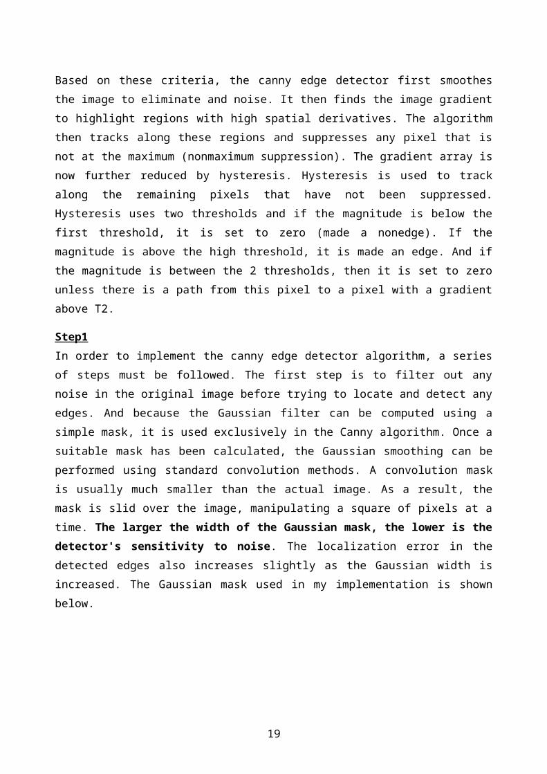
Based on these criteria, the canny edge detector first smoothes the image to eliminate and noise.

It then finds the image gradient to highlight regions with high spatial derivatives. The algorithm

then tracks along these regions and suppresses any pixel that is not at the maximum

(nonmaximum suppression). The gradient array is now further reduced by hysteresis. Hysteresis is

used to track along the remaining pixels that have not been suppressed. Hysteresis uses two

thresholds and if the magnitude is below the first threshold, it is set to zero (made a nonedge). If

the magnitude is above the high threshold, it is made an edge. And if the magnitude is between

the 2 thresholds, then it is set to zero unless there is a path from this pixel to a pixel with a

gradient above T2.

Step1

In order to implement the canny edge detector algorithm, a series of steps must be followed. The

first step is to filter out any noise in the original image before trying to locate and detect any

edges. And because the Gaussian filter can be computed using a simple mask, it is used

exclusively in the Canny algorithm. Once a suitable mask has been calculated, the Gaussian

smoothing can be performed using standard convolution methods. A convolution mask is usually

much smaller than the actual image. As a result, the mask is slid over the image, manipulating a

square of pixels at a time. The larger the width of the Gaussian mask, the lower is the detector's

sensitivity to noise. The localization error in the detected edges also increases slightly as the

Gaussian width is increased. The Gaussian mask used in my implementation is shown below.

16

Step2

After smoothing the image and eliminating the noise, the next step is to find the edge strength by

taking the gradient of the image. The Sobel operator performs a 2-D spatial gradient

measurement on an image. Then, the approximate absolute gradient magnitude (edge strength)

at each point can be found. The Sobel operator uses a pair of 3x3 convolution masks, one

estimating the gradient in the x-direction (columns) and the other estimating the gradient in the

y-direction (rows). They are shown below:

The magnitude, or EDGE STRENGTH, of the gradient is then approximated using the formula:

|G| = |Gx| + |Gy|

Step3

Finding the edge direction is trivial once the gradient in the x and y directions are known.

However, you will generate an error whenever sumX is equal to zero. So in the code there has to

be a restriction set whenever this takes place. Whenever the gradient in the x direction is equal to

zero, the edge direction has to be equal to 90 degrees or 0 degrees, depending on what the value

of the gradient in the y-direction is equal to. If GY has a value of zero, the edge direction will equal

0 degrees. Otherwise the edge direction will equal 90 degrees. The formula for finding the edge

direction is just:

theta = invtan (Gy / Gx)

17

Step4

Once the edge direction is known, the next step is to relate the edge direction to a direction that

can be traced in an image. So if the pixels of a 5x5 image are aligned as follows:

x x x x x

x x x x x

x x a x x

x x x x x

x x x x x

Then, it can be seen by looking at pixel "a", there are only four possible directions when

describing the surrounding pixels - 0 degrees (in the horizontal direction), 45 degrees (along the

positive diagonal), 90 degrees (in the vertical direction), or 135 degrees (along the negative

diagonal). So now the edge orientation has to be resolved into one of these four directions

depending on which direction it is closest to (e.g. if the orientation angle is found to be 3 degrees,

make it zero degrees). Think of this as taking a semicircle and dividing it into 5 regions.

18

Therefore, any edge direction falling within the yellow range (0 to 22.5 & 157.5 to 180 degrees) is

set to 0 degrees. Any edge direction falling in the green range (22.5 to 67.5 degrees) is set to 45

degrees. Any edge direction falling in the blue range (67.5 to 112.5 degrees) is set to 90 degrees.

And finally, any edge direction falling within the red range (112.5 to 157.5 degrees) is set to 135

degrees.

Step5

After the edge directions are known, nonmaximum suppression now has to be applied.

Nonmaximum suppression is used to trace along the edge in the edge direction and suppress any

pixel value (sets it equal to 0) that is not considered to be an edge. This will give a thin line in the

output image.

Step6

Finally, hysteresis is used as a means of eliminating streaking. Streaking is the breaking up of an

edge contour caused by the operator output fluctuating above and below the threshold. If a

single threshold, T1 is applied to an image, and an edge has an average strength equal to T1, then

due to noise, there will be instances where the edge dips below the threshold. Equally it will also

extend above the threshold making an edge look like a dashed line. To avoid this, hysteresis uses

2 thresholds, a high and a low. Any pixel in the image that has a value greater than T1 is

presumed to be an edge pixel, and is marked as such immediately. Then, any pixels that are

connected to this edge pixel and that have a value greater than T2 are also selected as edge

pixels. If you think of following an edge, you need a gradient of T2 to start but you don't stop till

you hit a gradient below T1. [11]

Figure 3-7 image before Canny edge detection [9] Figure 3-8 image after Canny edge detection [9]

19

3.2.3. Prewitt Operator

The Prewitt edge detection masks are one of the oldest and best understood methods of detecting edges in images. Basically, there are two masks, one for detecting image derivatives in X and one for detecting image derivatives in Y. To find edges, a user convolves an image with both masks, producing two derivative images. The strength of the edge at any given image location is then the square root of the sum of the squares of these two derivatives.

In practice, usually one thresholds is used in Prewitt edge detection, in order to produce a discrete set of edges. Bellowing figures show a source image and the thresholded result of Prewitt edge detection: [12]

Figure 3-9 image before Prewitt edge detection [12] Figure 3-10 image after Prewitt edge detection [12]

3.2.4.Roberts' Cross Operator

According to Roberts, an edge detector should have the following properties: the produced edges

should be well-defined, the background should contribute as little noise as possible, and the

intensity of edges should correspond as close as possible to what a human would perceive. With

these criteria in mind and based on then prevailing psychophysical theory Roberts proposed the

following equations:

20

Where x is the initial intensity value in the image, z is the computed derivative and i,j represent

the location in the image. [13]

In order to perform edge detection with the Roberts operator we first convolve the original

image, with the following two kernels:

Figure 3-11 Roberts Cross masks [13]

Figure 3-12 image before Roberts' edge detection[13] Figure 3-13 image after Roberts' edge detection[13]

Roberts' Cross is still in use due to the speed of computation, but performance compared to the

other method is poor, with noise sensitivity a significant problem.

3.2.5.Conclusion

Let’s compare with these edge detection algorithms above:

21

Grayscale image of a brick wall & a bike rack

Figure 3-11 compare with Robert Cross, Sobel, and Prewitt operator [13]

We notice that the lines corresponding to edges have become thicker compared with the Roberts

Cross output due to the increased smoothing of the Sobel operator and Prewitt operator.

To compare with Robert Cross, Sobel and Canny operator we use the image below which

contains Gaussian noise with a standard deviation of 15.

Figure 3-12 Original image to compare with Robert Cross, Sobel, and Canny operator [16]

22

Figure 3-13 Figure 3-14 Figure 3-15Robert Cross operator [17] Sobel operator [18] Canny operator [16]

Neither the Roberts Cross nor the Sobel operator are able to detect the edges of the object while removing all the noise in the image. Applying the Canny operator using a standard deviation of 1.0 yields a very clear edge image that all of the edges have been detected and almost all of the noise has been removed. The Gaussian smoothing in the Canny edge detector fulfills two purposes: first it can be used to control the amount of detail that appears in the edge image and second, it can be used to suppress noise. After compared the above edge detection algorithms, I choose Canny edge detection for my project, because this algorithm can effectively suppress noise, retaining continuous, clear edges.

3.3. Number Plate Localization

Registration marks on number plates in Ireland issued since 1987 have the format YY-CC-SSSSSS

where the components are:

* YY — a 2-digit year (e.g. 87 for 1987; 05 for 2005)

* CC — a 1- or 2-character county identifier (e.g. D for Dublin; SO for Sligo).

* SSSSSS — a 1- to 6-digit sequence number, starting with the first vehicle registered in the

county that year. [14]

23

Figure 3-16 example of current standard Irish number plate [15]

Figure 3-17 example of current standard Irish number plate [14]

The Irish number plate is white background with

black characters on it and surrounded by a black border having a stroke width of 5 millimeters.

The external size of the plate shall be 520 millimeters in width and 110 millimeters in height. The

flag of the European Communities with letters IRL is in the left side of plate in blue background.

The characters shall have a height of 70 millimeters and a stroke width of 10 millimeters. The

width of each character (other than the letter “I” or the number “1”) shall be not less than

36millimetres and not more than 50 millimeters. The distances between adjoining letters and

adjoining figures shall be not less than 8 millimeters [15].

24

Figure 3-18 Ireland county code [14]

3.3.1.Number Plate Isolation

After applying edge detection algorithm, the edge information of the area which contains the

number plate is much richer than the other areas. This is because there are many characters

which contains a lot of strokes internal the number plate. At the same time, number plate area is

a relatively rectangle surrounded by straight lines. Therefore, we first define a window which has

the same ratio of length and width of number plate but larger than it. And then move this

window around in the image and count the number of white pixel within the window, because

the edge information is most concentrated in the sub-image which contains the number plate,

we can identify that the sub-image which has the maximum number of white pixel is the area

contains number plate.

In the following figure, the red rectangular is a slide-window which moves around in the picture

until find the sub-image contains the maximum number of white pixel and this sub-image usually

contains the number plate.

Figure 3-19 using slide-window to isolate plate

At first, identify the top and bottom boundaries of number plate. This algorithm scans line by line

from top to bottom, count the times of pixel changes (from 0 to 1 or from 1 to 0) between

adjacent pixels. When the time of changes in one certain line is greater than a threshold value

and the same as the following n lines, we can assume this line is the top line of the number plate.

And then continue scans line by line until find a certain line has the times of changes less than

threshold value and assume this line is the bottom line of the number plate.

25

Define an array with value 0 for its entire element to record the times of gray-scale changes in

each horizon line, the length of the array equals to the height of the sub-image.

Scan the sub-image line by line from top to bottom, count the time of gray-scale changes in each

line, if the value of time > threshold then stores 1 into the corresponding position of the array.

After the whole sub-image scanned, check the array from its first element, if there are n

continues elements have value 1 then we can assume the line related to the first element is the

top line of the number plate. The bottom line can be found in same method by check the array

from its last element.

Figure 3-20 original image Figure 3-21 image after locate top and bottom boundary

In above figure, the number plate has 8 characters, each character at least has two times of pixel

changes when a line scans cross the plate, so set the threshold value as 16. The top and bottom

border of the plate has been removed.

The second step is Identify the left and right boundaries of number plate.

Define an array with value 0 for its elements to store the projection information of each vertical

line.

Scan the sub-image line by line in vertical direction. If the number of white pixel > n, then change

the value of the corresponding element in the array into 1.

After the whole sub-image scanned, first check the array from its first element until finds the n

continues elements have value 0, and assume the line related to the first element which has

value 1 after these elements is the left boundary of the number plate. The right boundary can be

found by in same method by check the array from its last element.

3.3.2. Number Plate Localization Based on HSV Color Space

There is always a blue rectangle part with the flag of the European Communities and letters “IRL”

on the left side of the number plate. So, after isolate the number plate, we can confirm whether

26

the sub-image contains the number plate by check whether there is a blue rectangle in the left

side of the sub-image. Because the height of the blue rectangle is also the height of the number

plate, so the top line and the bottom line is also the top and bottom boundary of the number

plate. Also because the aspect ratio of number plate is fixed, so the length of the plate can be

calculated after we know the height of the plate.

It is very complicate and time-consuming to identify colors in RGB color space, so we use HSV

color space instead.

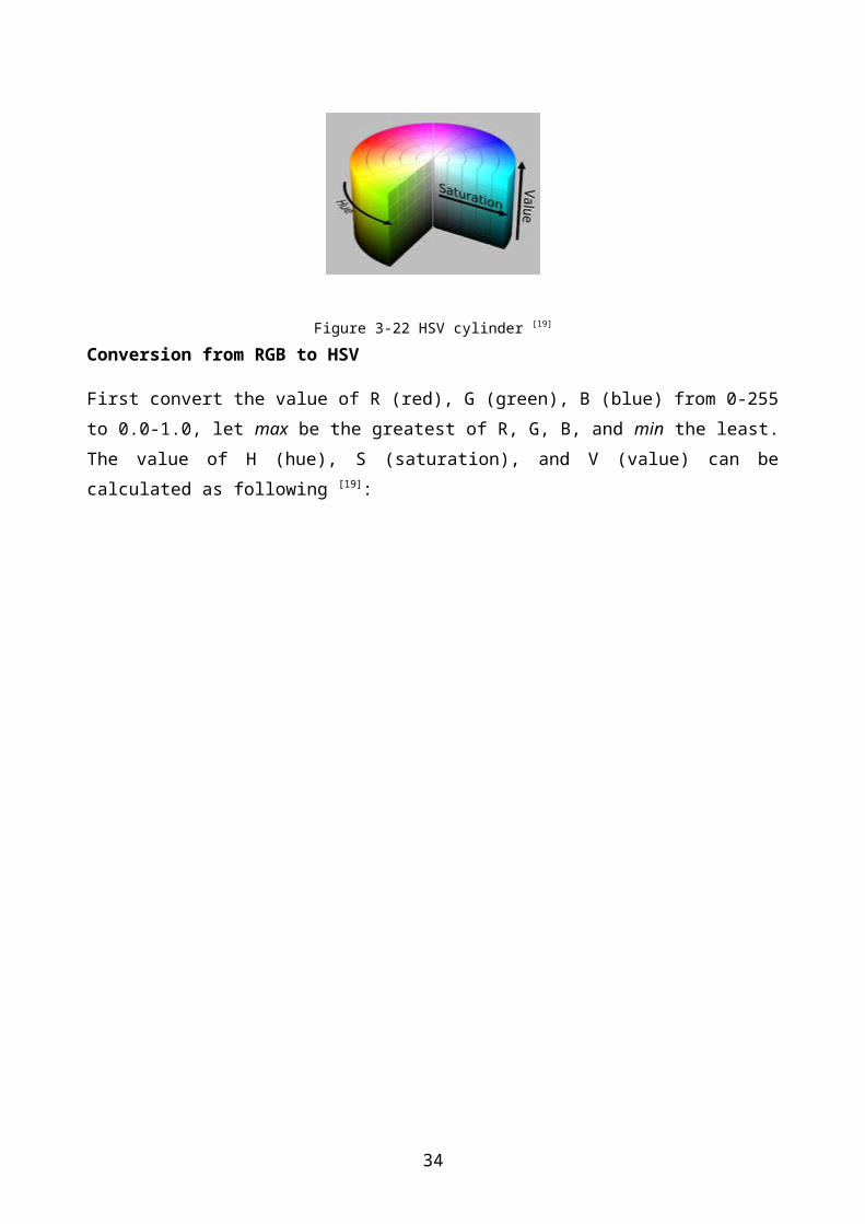
HSV can be thought of as describing colors as points in a cylinder (called a color solid) whose

central axis ranges from black at the bottom to white at the top, with neutral colors between

them. The angle around the axis corresponds to “hue”, the distance from the axis corresponds to

“saturation”, and the distance along the axis corresponds to “lightness”, “value” or “brightness” [19].

Figure 3-22 HSV cylinder [19]

Conversion from RGB to HSV

First convert the value of R (red), G (green), B (blue) from 0-255 to 0.0-1.0, let max be the

greatest of R, G, B, and min the least. The value of H (hue), S (saturation), and V (value) can be

calculated as following [19]:

27

Find the blue rectangle area in the sub-image

After convert RGB to HSV, scans the whole sub-image to find the blue rectangle area by check the

value of H (hue) in each pixel.

Figure 3-23 hue region for different value [19]

Value of H (0-360) Hue Region0-60 Red-Yellow60-120 Yellow-Green120-180 Green-Cyan180-240 Cyan-Blue240-300 Blue-Magenta300-360 Magenta-Red

28

3.4 Character Segmentation

The format of Irish number plate is YY-CC-SSSSSS where YY is a 2 digit year, CC a 1 or 2 letter

county identifier and SSSSSS is a 1 to 6 digit sequence number. So the length of number plate is

from 4 characters (2 numbers + 1 letter +1 number) to 10 characters (2 numbers + 2 letters + 6

numbers). There are always gaps between characters in number plate, so vertical projection

method can also be used to separate characters.

3.4.1 Character Segmentation with Vertical Projection

First scans the number plate area line by line in vertical direction, count the number of white

pixel in each line. Because the projection of numbers and letters are continues, then if the

number of white pixel in n adjacent lines less than a threshold value, we can assume these lines is

a gap area between characters.

Figure 3-24 Original image of a number plate [20]

29

Figure 3-25 vertical projection of a number plate [20]

Define an array with value 0 for its elements to store the projection information of each vertical

line.

Scan the sub-image line by line in vertical direction. If the number of white pixel > n, then change

the value of the corresponding element in the array into 1.

After the whole sub-image scanned, check the array from its first element, if one element has

value 0 and next element has value 1, we can assume these lines are the beginning position of a

character, or vice versa.

3.4.2 Character Segmentation with Log-Gabor filters

In order to segment characters properly, we need to have simultaneously spatial information to

locate the character separation in the image and frequency information to use gray level

variation to detect these separations. Gabor filters could be a choice to address this problem.

30

Gabor filters have been extensively used to characterize texture and more specifically in our

context to detect and localize text into an image. In this aim, Gabor filters are quite time

consuming because several directions and frequencies must be used to handle the variability in

character sizes and orientations. Gabor filters present a limitation in the bandwidth where only

bandwidth of 1 octave maximum could be designed. Log-Gabor filters, proposed by Field,

circumvent this limitation. They always have a null DC component and can be constructed with

arbitrary bandwidth and the bandwidth can be optimized to produce a filter with minimal spatial

extent.

Log-Gabor filters in frequency domain can be defined in polar coordinates by H(f, θ) = Hf × Hθ

where Hf is the radial component and Hθ, the angular one:

with f0, the central frequency, θ0, the filter direction, σf , which defines the radial bandwidth B in

octaves with B = and σθ, which defines the angular bandwidth

As we are looking for vertical separation between characters, we use only two directions for the

filter, the horizontal and the vertical one. Hence, for each directional filter, we got a fixed angular

bandwidth of ΔΩ = Π/2. Log-Gabor filters are not really strict with directions and defining only

two directions enables to handle italic and/or misaligned characters.

Only two parameters remain to define, f0 and σf, used to compute the radial bandwidth.

The central frequency f0 is used to handle gray level variations to detect separation between

characters. It is quite logical to get a central frequency close to the inverse of the thickness of

characters to get those variations. Nevertheless, the thickness of characters can not be very

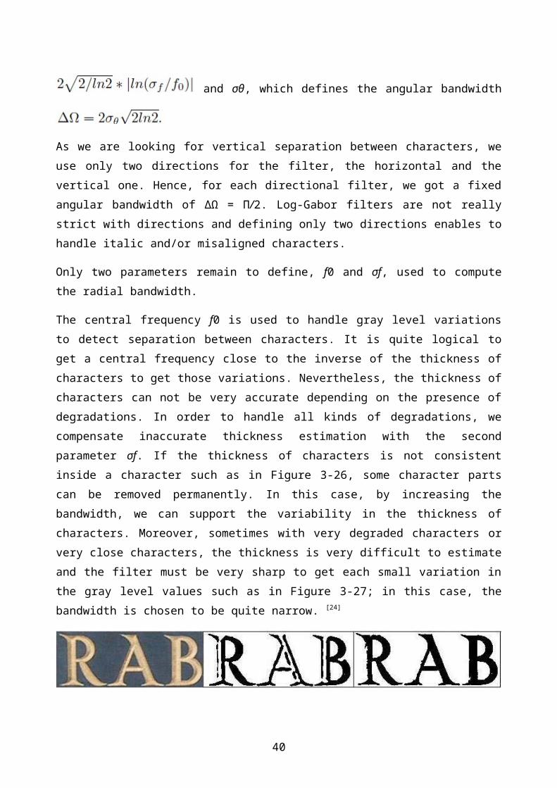
accurate depending on the presence of degradations. In order to handle all kinds of degradations,

we compensate inaccurate thickness estimation with the second parameter σf. If the thickness of

characters is not consistent inside a character such as in Figure 3-26, some character parts can be

removed permanently. In this case, by increasing the bandwidth, we can support the variability in

the thickness of characters. Moreover, sometimes with very degraded characters or very close

characters, the thickness is very difficult to estimate and the filter must be very sharp to get each

31

small variation in the gray level values such as in Figure 3-27; in this case, the bandwidth is

chosen to be quite narrow. [24]

Figure 3-26 from left to right: original image, segmentation with misestimated thickness, segmentation with the same

thickness corrected by a larger bandwidth [24]

Figure 3-27 Original image (top left), binary version (top right), segmentation with large bandwidth (bottom left),

segmentation with narrow bandwidth (bottom right) [24]

3.4. Character Recognition

3.4.1. Projection Method

This method first each character bitmap is projected in both vertical and horizontal direction, and

then count number of peaks in vertical direction, the number of peaks in horizontal direction, the

number of end points of the character and the number of junctions of the character.

32

Figure 3-28 vertical and horizontal projection for character “6” [22].

The character bitmap might contain all characters. The algorithm starts with determining the

number of peaks in the vertical direction and the number of peaks in horizontal direction.

The characters {5, 6, 8, 9, B, G} all have 2 vertical peaks and 3 horizontal peaks. The other

characters cannot be contained in this bitmap. The second step of the recognition algorithm is

determined by the result of the first step. In this case, the algorithm determines the number of

endpoints and junctions.

From the remaining characters {5, 6, 8, 9, B, G}, the characters {6, 9} are the only characters with

1 endpoint and 1 junction. The third step of the classification algorithm is dependent on the

result of the second step. In this case, the algorithm determines the row position of the endpoint

with respect to the junction.

From the remaining characters {6, 9} is {6} the only character that has an endpoint that is higher

than its junction.

33

Number of peaks in vertical direction: 2

Number of peaks in horizontal direction: 3

Number of end point: 1

Number of junction point: 1

Conclusion: the character contained in this bitmap is a 6. [22]

3.4.2. Recognizing of characters using neural networks

The character sequence of license plate uniquely identifies the vehicle. It is proposed to use

artificial neural networks for recognizing of license plate characters, taking into account their

properties to be as an associative memory. Using neural network has advantage from existing

correlation and statistics template techniques that allow being stable to noises and some position

modifications of characters on license plate. [25]

Figure 3-29 The topology of the designed neural network [26]

The training process has been completed approximately in 20000 iterations. When off-line

training is completed, a neural network is designed using the obtained weights as seen in figure

3-29.

34

3.4.3. Grid Feature Method

In this method, two features are extracted. The first one grid feature is extracted by divide the

bitmap into 3*3= 9 small grids and counts the white pixels in each grid to form a 9-dimentinal

vector. Another one is cross-point feature which get by drawing two vertical lines onto the

bitmap to divide it into three equal parts in vertical direction, and draw two horizontal lines onto

the bitmap to divide it into three equal parts in horizontal direction, then count the number of

cross-point for each line to form a 4-dimensional vector. Connect the two vectors together to

form a 13-dementional vector. Use this method we first create vector templates for all the

characters. So, when need to identify a character, first get the 13-dementional vector from the

bitmap and compare it with the templates to find the most similar template [21].

The following figure gives an example of grid feature method for character “6”.

Figure 3-30 applying grid feature method on character “6”

Figure 3-31 analysis transfer detected character by matrix mapping [23]

35

Apply gird feature method on character “6” to form a 13-demantional vector:

Dimensionalnumber

1 2 3 4 5 6 7

value 24 36 10 52 32 40 31Dimensional number

8 9 10 11 12 13

value 28 38 3 3 1 2

3.4.4. Conclusion

the problems of projection method that are very much alike is the characters B and 8, 0 and

D, and 2 and Z are often not distinguishable, but the characters S and 5, V and Y, and C and G are.

To avoid these problems we can first classify the character. The only letters in number plate is the

1 or 2 character county identifier, so we can first divide the plate to three parts: 2-digit year part,

1- or 2-letter part and 1- to 6-digit part, and then recognize them part by part, this can improve

the recognition rate.

Grid Feature Method makes full use of the distribution information of pixels in images. On the

other hand, it does not require thinning the characters, thus avoiding the broken and adhesions

of strokes caused by thinning, so that increased the rate of character recognition.

4.Programming Languages

4.1. Programming Language

Java

Java was launched by SUN company during SUN WORLD 95 MEETING. Though java is not an

official sequel of C++, it uses a large member of grammar from C++. It threw away a lot of the

complex function of C++ to form a compact and easy-learned language. Unlike C++, Java

mandatory object-oriented programming. "Virtual machine" mechanism, garbage collection and

no pointer make it easy to achieve a reliable application.

C

C language is more advanced than assembly language. It uses a process-oriented programming

method. At the same time, it is kind of machine-oriented programming language and still very

close to assembly language. It is one of the most efficient high-level programming languages. Its

36

platform compatibility is very good, and almost all systems have the C language compiler. It is

suitable for developing operating system and other programming which direct operate hardware

and it is also suitable for all kinds of programmer, especially for beginners.

C++

With the continuous expansion of the size of the software, people found that the traditional use

of: “data structure + algorithm” structured programming model has been difficult to adapt to the

development of the software. At this time, the object-oriented programming idea was attracted

programmers’ attention. The first C + + languages was published by AT & T's Bell Labs in 1985. It

is based on C language, and adds the object-oriented thinking. It is support three programming

modes: process-oriented, object-oriented and template. It has become one of the most popular

programming languages.

Pascal

Pascal language was designed by Nicolas Wirth in the early 1970s. Pascal was originally strictly

designed to be used in teaching, eventually, a large number of advocates to promote it into the

commercial programming. Compared to the previous programming language, Pascal language is

a structured language, it has a wealth of data types and control structure, and it is easy to

understand, it is particularly suitable for teaching. Pascal language is also a self-compiled

language, which greatly enhanced its reliability.

C#

C# is an object-oriented language which works with Microsoft .NET framework, and it integrates

the advantages of a lot of other language, like Java, C++, VB and Delphi. It not only can be used

for the development of WEB services, but also the development of powerful system-level

program.

Comparison:

Language Name CAdvantage 1) Process-oriented development and function-centred. Simple and

effective.

2) Machine-oriented, so that users can manipulate the machines more

37

efficient.

3) High-performance, widely used in all kinds of computer fields. Very

effective for simple project.

Disadvantage

1) The ability of package data is week, grammar is not strict restrictions,

which make the C language a lot of weaknesses in data safety.

2) Control the machine too strong means depends on machine too strong.

Because of too concentrate on efficiency, when we use C to

programming, we should consider the machines mach more than the

problem itself.

3) Unsuitable for develop large project.

PortabilityThe portability of C language limited to process control, memory management and simple document handling. Other things related to the relevant platform.

Language Name C++

Advantage1) Much better than C when develop large project. 2) Has a good support for object-oriented mechanism. 3) Universal data structure.

Disadvantage1) Very large and complex.2) Grammar is not strict restrictions as C language. 3) Slower than C.

PortabilityMuch better than the C language, but still not very optimistic. Because it has the same shortcomings with the C language.

Language Name Pascal

Advantage1) Easy to learn.2) Has a very good platform (Delphi).

Disadvantage The standard of language is not accepted by compiler developers.Portability Very poor. Language functions changes in different platform.

Language Name JavaDisadvantage 1) Binary code can be ported to other platforms.

2) Application can run on the webpage.

38

3) Its class libraries are very standard and extremely strong. 4) Automatic allocation and garbage collection can avoid leakage of resources.

DrawbackUse a "virtual machine" to run portable byte code rather than the local machine code, its compile and running speed are much slower than other local application.

PortabilityThe best. Low-level code has a very high portability, but a lot of new features are unstable in some platform.

Language Name C#

Advantage1) Simple, easy to learn and understand.2) No pointer.3) Garbage collector can manage memory automatically.

Disadvantage Only few components and libraries can be used now.

PortabilityNot very good. Software developed by using C# requires .NET runtime as basis, and it only can work in Windows system.

4.2. Conclusion

After compare the advantages, disadvantages and portability of the above language, I decide to

use Java as my programming language. Because Java not only has extremely powerful class

libraries and the best portability, but also very easy to use and I am good at java. So, I would like

to use Java as my programming language.

39

5.NPR System Conclusion

There are lots of different ways are found to implement each part of the NPR system after the

two months research. But only few of them need to be choosing for my project. At first, I will use

luminosity method for converting image to grayscale. Because the other methods are tend to

reduce contrast. The luminosity method works best overall. Secondly, for better edge detection,

using Gaussian blur to process image smoothing. Gaussian smoothing will contain in canny

operator which I choose for edge detection. After compare with other operator, we know that

canny operator can effectively suppress noise, retaining continuous, clear edges. Following edge

detection, we do vertical projection for character segmentation. Finally, Grid Feature Method

will take the responsibility of character recognition. Cause it makes full use of the distribution

information of pixels in images. On the other hand, it does not require thinning the characters,

thus avoiding the broken and adhesions of strokes caused by thinning, but projection method

cannot.

6.Bibliography

[1] http://en.wikipedia.org/wiki/Automatic_number_plate_recognition

[2] http://www.vigilantvideo.com/CarDetector_Fixed.htm

[3] http://www.filebuzz.com/fileinfo/36485/Intertraff_Parking_Manager.html

[4] http://www.traffictechnologytoday.com/news.php?NewsID=8072

[5] http://www.flickr.com/photos/rockmanzym/4323307686/

[6] http://www.johndcook.com/blog/2009/08/24/algorithms-convert-color-grayscale/

[7] http://en.wikipedia.org/wiki/Gaussian_blur

[8] http://en.wikipedia.org/wiki/Laplace_operator

40

[9] http://en.wikipedia.org/wiki/Sobel_operator

[10] http://en.wikipedia.org/wiki/Edge_detection

[11] http://www.pages.drexel.edu/~weg22/can_tut.html

[12] http://www.cs.colostate.edu/cameron/prewitt.html

[13] http://en.wikipedia.org/wiki/Roberts_Cross

[14] http://en.wikipedia.org/wiki/Vehicle_registration_plates_of_Ireland

[15] http://www.craigsplates.ie/irish-number-plate-law

[16] http://homepages.inf.ed.ac.uk/rbf/HIPR2/canny.htm

[17] http://homepages.inf.ed.ac.uk/rbf/HIPR2/roberts.htm

[18] http://homepages.inf.ed.ac.uk/rbf/HIPR2/sobel.htm

[19] http://en.wikipedia.org/wiki/HSV_color_space

[20] http://theblogfor.net/index.php/2010/01/character-segmentation-from-the-image-1-line/

[21] Seong Whan Lee, Dong-June Lee, Hee-Seon Park. New methodology for ray-scale character

segmentation and recognition. IEEE Transactions on pattern Analysis and Machine

Intelligence, 1996, 1045-1050

[22] Lee J Nelson. Recent Advances in License Plate Recognition. Advanced Imaging, 2002, 18-21,

53

[23] http://www.codeproject.com/KB/recipes/UnicodeOCR.aspx

[24] http://tcts.fpms.ac.be/publications/papers/2006/icpr2006_cmtbg.pdf

[25] http://www.jatit.org/volumes/research-papers/Vol12No1/5Vol12No1.pdf

[26] http://www.emo.org.tr/ekler/c3dee15d074d783_ek.pdf

41