Soft Computing-based Life-Cycle Cost Analysis Tools for

Soft Computing-based Life-Cycle Cost Analysis Tools for Transportation Infrastructure Management

Chen Chen

Dissertation submitted to the faculty of the Virginia Polytechnic Institute and State University in partial fulfillment of the requirements for the degree of

Doctor of Philosophy

In Civil and Environmental Engineering

Gerardo W. Flintsch, Committee Chair Imad L. Al-Qadi James W. Bryant Amara Loulizi

Antonio A. Trani Linbing Wang

June 7th, 2007 Blacksburg, Virginia

Keywords: Life-cycle Costs Analysis (LCCA), Pavement Management, Fuzzy Logic

System, Neuro-fuzzy System, Project Selection

Copyright 2007, Chen Chen

Soft Computing-based Life-Cycle Cost Analysis Tools

for Transportation Infrastructure Management

Chen Chen

ABSTRACT Increasing demands, shrinking financial and human resources, and increased

infrastructure deterioration have made the task of maintaining the infrastructure systems

more challenging than ever before. Life-cycle cost analysis (LCCA) is an important tool

for transportation infrastructure management, which is used extensively to support

project level decisions, and is increasingly being applied to enhance network level

analysis. However, traditional LCCA tools cannot practically and effectively utilize

expert knowledge and handle ambiguous uncertainties.

The main objective of this dissertation was to develop enhanced LCCA models using soft

computing (mainly fuzzy logic) techniques. The proposed models use available “real-

world” information to forecast life-cycle costs of competing maintenance and

rehabilitation strategies and support infrastructure management decisions.

A critical review of available soft computing techniques and their applications in

infrastructure management suggested that these techniques provide appealing alternatives

for supporting many of the infrastructure management functions. In particular, LCCA

often utilizes information that is uncertain, ambiguous and incomplete, which is obtained

from both existing databases and expert opinion. Consequently, fuzzy logic techniques

were selected to enhance life-cycle cost analysis of transportation infrastructure

investments because they provide a formal approach for the effective treatment of these

types of information.

The dissertation first proposes a fuzzy-logic-based decision-support model, whose

inference rules can be customized according to agency’s management policies and expert

opinion. The feasibility and practicality of the proposed model is illustrated by its

iii

implementation in a life-cycle cost analysis algorithm for comparing and selecting

pavement maintenance, rehabilitation and reconstruction (MR&R) policies.

To enhance the traditional probabilistic LCCA model, the fuzzy-logic-based model is

then incorporated into the risk analysis process. A fuzzy logic approach for determining

the timing of pavement MR&R treatments in a probabilistic LCCA model for selecting

pavement MR&R strategies is proposed. The proposed approach uses performance

curves and fuzzy-logic triggering models to determine the most effective timing of

pavement MR&R activities. The application of the approach in a case study

demonstrates that the fuzzy-logic-based risk analysis model for LCCA can effectively

produce results that are at least comparable to those of the benchmark methods while

effectively considering some of the ambiguous uncertainty inherent to the process.

Finally, the research establishes a systematic method to calibrate the fuzzy-logic based

rehabilitation decision model using real cases extracted from the Long Term Pavement

Performance (LTPP) database. By reinterpreting the model in the form of a neuro-fuzzy

system, the calibration algorithm takes advantage of the learning capabilities of artificial

neural networks for tuning the fuzzy membership functions and rules. The practicality of

the method is demonstrated by successfully tuning the treatment selection model to

distinguish between rehabilitation (light overlay) and do-nothing cases.

iv

ACKNOWLEDGEMENTS

I would like to express my sincere gratitude to Dr. Gerardo W. Flintsch for his guidance,

encouragement, and support during this research. Special thanks are also given to the

committee members, Dr. Imad Al-Qadi, Dr. James Bryant, Dr. Amara Loulizi, Dr.

Antonio Trani, and Dr. Linbing Wang for the time and expertise contributed to the

enhancement of this research. Dr. Dusan Teodorovic, as a former committee member, is

greatly appreciated for his guidance on the theory of soft computing techniques.

Sincere gratitude goes to my parents, Xuean Chen and Mei Zhang, my brother, Guang

Chen, and all other members of my family for their love and encouragement. Their pride

in my accomplishments guided me throughout the best and the worst moments of my

work from 7,000 miles away.

Also to all my friends at Virginia Tech and Blacksburg, who made my life as a Hokie

most enjoyable and honorable, goes my sincere thanks.

Finally, this dissertation is dedicated to my wife, Yinli, for her love, belief in me, and

constant support. Her guidance, patience and understanding helped me finalize this

research.

v

Table of Contents

Chapter 1: Introduction ................................................................................................... 1 Background..................................................................................................................... 2

Life-Cycle Cost Analysis ............................................................................................. 2 LCCA in Transportation ............................................................................................. 3

Problem Statement .......................................................................................................... 5 Research Objective ......................................................................................................... 5 Organization of the Dissertation ..................................................................................... 6 Results and Significance................................................................................................. 8 References....................................................................................................................... 9

Chapter 2: Soft Computing Applications in Infrastructure Management................ 10 Abstract......................................................................................................................... 11 Introduction................................................................................................................... 12 Infrastructure Management Systems ............................................................................ 13 Functional Framework for Infrastructure Asset Management...................................... 15 Soft Computing............................................................................................................. 16

Artificial neural networks ......................................................................................... 18 Fuzzy logic systems ................................................................................................... 18 Genetic Algorithms ................................................................................................... 19 Hybrid Systems.......................................................................................................... 20

Soft Computing Applications in Infrastructure Management....................................... 20 Condition Assessment ............................................................................................... 22 Performance Prediction............................................................................................ 24 Need analysis ............................................................................................................ 24 Prioritization............................................................................................................. 25 Optimization.............................................................................................................. 26

Implementation Issues .................................................................................................. 27 Summary and Conclusions ........................................................................................... 29 Acknowledgement ........................................................................................................ 30 References..................................................................................................................... 31

Chapter 3: Fuzzy Logic-Based Life-Cycle Costs Analysis Model for Pavement and Asset Management .......................................................................................................... 38

Abstract......................................................................................................................... 39 Introduction................................................................................................................... 40 Engineering economic analysis .................................................................................... 41 Soft computing applications for Pavement Management ............................................. 45

Utilizing Soft Computing for Engineering Economic Analysis................................. 46 Fuzzy Logic Systems ................................................................................................. 47

vi

Fuzzy Logic-Based LCCA Algorithm.......................................................................... 48 Agency Costs Model.................................................................................................. 49 User Costs Considerations ....................................................................................... 50

Case Study .................................................................................................................... 51 Decision Making Model............................................................................................ 51 MR&R Policies ......................................................................................................... 52

Discussion..................................................................................................................... 57 Conclusion .................................................................................................................... 57 References..................................................................................................................... 58

Chapter 4: Fuzzy Logic Pavement Maintenance and Rehabilitation Triggering Approach for Probabilistic Life-Cycle Cost Analysis.................................................. 61

Abstract......................................................................................................................... 62 Introduction................................................................................................................... 63 Objective....................................................................................................................... 65 Life-cycle cost analysis................................................................................................. 66

Common Assumptions............................................................................................... 66 Deterministic LCCA.................................................................................................. 67 Probabilistic LCCA................................................................................................... 67

Uncertainties in LCCA Inputs ...................................................................................... 68 Discount Rate............................................................................................................ 70 Initial Construction Costs ......................................................................................... 70 Rehabilitation Costs.................................................................................................. 71 Rehabilitation Timings.............................................................................................. 72 Potential Error Sources in Probabilistic LCCA ....................................................... 73

Fuzzy-logic-based LCCA Algorithm............................................................................ 74 Fuzzy Logic Systems ................................................................................................. 74 Determination of Rehabilitation Timing................................................................... 75

Comparative case study ................................................................................................ 77 Distributions of Input Variables ............................................................................... 79 Performance Models and Decision Models.............................................................. 80 LCCA Results ............................................................................................................ 81 Sensitivity Analysis.................................................................................................... 84

Summary and conclusions ............................................................................................ 86 Future enhancement ...................................................................................................... 87 Reference ...................................................................................................................... 88

Chapter 5: Calibrating Fuzzy-Logic-based Rehabilitation Decision Models Using LTPP database ................................................................................................................ 90

Abstract......................................................................................................................... 91 Introduction................................................................................................................... 92 Objective....................................................................................................................... 93

vii

Fuzzy-logic-based decision model................................................................................ 94 Data Preparation ........................................................................................................... 95

Geographical Area of Interest .................................................................................. 96 Pavement Condition Indicators ................................................................................ 96 Rehabilitation Treatments......................................................................................... 97 Deficient Records...................................................................................................... 97 Building Dataset for Calibration.............................................................................. 97

Design of Fuzzy logic systems ..................................................................................... 99 Membership Functions............................................................................................ 100 Inference Rules........................................................................................................ 101 Fuzzy Basis Functions............................................................................................. 102 Steepest Descent Method ........................................................................................ 103 Tuning Fuzzy Logic Systems ................................................................................... 103

Model Calibration ....................................................................................................... 104 Neural Fuzzy System............................................................................................... 106 Calibrating the Decision-support Models .............................................................. 107

Discussion................................................................................................................... 111 Data Preparation.................................................................................................... 112 Architecture Design of Fuzzy Logic Systems .......................................................... 112 Impacts of Distress(es) on Rehabilitation Decision................................................ 113

Summary and conclusions .......................................................................................... 113 References................................................................................................................... 115

Chapter 6: Summary, Conclusions and Future Works............................................. 117 Findings ...................................................................................................................... 118 Conclusions................................................................................................................. 119 Implementation Issues ................................................................................................ 120 Recommendations and Suggestions for Future Research........................................... 121

Appendix A: Matlab Scripts ........................................................................................ 123 Traditional Deterministic LCCA Model..................................................................... 124 Traditional Probabilistic LCCA Model ...................................................................... 130 Fuzzy-Logic-based LCCA Model .............................................................................. 142 Calibration Algorithm for Fuzzy-logic-based Decision Support Models................... 154

viii

List of Tables Chapter 2: Soft Computing Applications in Infrastructure Management

Table 2.1. Summary of AI and Soft Computing Applications in Infrastructure Management.................................................................................................................. 21 Table 2.2. Soft Computing Technique and Their Applicability for Asset Management...................................................................................................................................... 28

Chapter 3: Fuzzy Logic-Based Life-Cycle Costs Analysis Model for Pavement and Asset Management

Table 3.1. Advantages of the main soft computing techniques (after Flintsch 2003a). 46 Table 3.2. Example of fuzzy logic-based project selection model ............................... 53 Table 3.3. Cost and effect of the MR&R treatments considered.................................. 54 Table 3.4. Results obtained with the fuzzy logic-based LCCA model......................... 55

Chapter 4: Fuzzy Logic Pavement Maintenance and Rehabilitation Triggering Approach for Probabilistic Life-Cycle Cost Analysis

Table 4.1. Engineering Design Parameters for Alternatives A and B .......................... 77 Table 4.2. Input Variables for Different LCCA Models and Assumed Statistics for Each Variable................................................................................................................ 78 Table 4.3. Correlation Sensitivity for Alternatives A and B ........................................ 86

Chapter 5: Calibrating Fuzzy-Logic-based Rehabilitation Decision Models Using LTPP Database

Table 5.1. Rehabilitation Cases .................................................................................... 98 Table 5.2. Inference Rule Bases of the Decision Model ............................................ 102 Table 5.3. Fuzzy-Logic-based Decision Model.......................................................... 111

ix

List of Figures Chapter 2: Soft Computing Applications in Infrastructure Management

Figure 2.1. Generic Asset Management Framework (after FHWA 1999) ................... 15 Figure 2.2. Intelligent Infrastructure Asset Management System Framework............. 15 Figure 2.3. Example of Neuro-Fuzzy System............................................................... 23

Chapter 3: Fuzzy Logic-Based Life-Cycle Costs Analysis Model for Pavement and Asset Management

Figure 3.1. Pavement management system framework (Flintsch, 2003a).................... 41 Figure 3.2. Membership functions for the various pavement variables considered. .... 48 Figure 3.3. Fuzzy logic-based LCCA framework......................................................... 50 Figure 3.4. Fuzzy logic-based project selection algorithm........................................... 52 Figure 3.5. Priority progression for the medium overlay policy .................................. 55 Figure 3.6. Priority progression for the reconstruction policy...................................... 55 Figure 3.7. Expenditure stream for the medium overlay policy. .................................. 56 Figure 3.8. Expenditure stream for the reconstruction policy. ..................................... 56

Chapter 4: Fuzzy Logic Pavement Maintenance and Rehabilitation Triggering Approach for Probabilistic Life-Cycle Cost Analysis

Figure 4.1. Probabilistic LCCA result example............................................................ 64 Figure 4.2. Relationship map of LCCA input variables and parameters ...................... 69 Figure 4.3. (a) Fuzzy-logic MR&R triggering algorithm; (b) Solution surfaces produced by the fuzzy logic models ............................................................................. 76 Figure 4.4. Expenditure stream diagram for alternative A and B using deterministic method .......................................................................................................................... 82 Figure 4.5. Risk profile of PV for alternatives A and B using (a) threshold trigger model and (b) fuzzy-logic triggering model ................................................................ 83 Figure 4.6. Probability of rehabilitation timing using (a) threshold trigger model and (b) fuzzy-logic triggering model................................................................................... 85

Chapter 5: Calibrating Fuzzy-Logic-based Rehabilitation Decision Models Using LTPP database

Figure 5.1. Fuzzy Logic based Decision Model (Chen et al., 2004) ............................ 95 Figure 5.2. Procedure for Extracting Training Data from LTPP Database .................. 96 Figure 5.3. Data Extracted from LTPP Database ......................................................... 98 Figure 5.4. Reinterpreting Decision Model in the form of Neural Fuzzy System...... 105 Figure 5.5. Cases of Overlay Treatment ..................................................................... 110 Figure 5.6. Number of cases with mistaken decisions decreasing through multi-pass calibration ................................................................................................................... 110

1

CHAPTER 1: INTRODUCTION

2

BACKGROUND

Transportation systems provide mobility, access, opportunity and choice for people. Sound

transportation infrastructure systems play a vital role in encouraging a productive and competitive

national economy (GAO, 2000). With 8,315,121 lane-miles of roadway, 593,813 bridges, 19,820

airports and more than 12,000 miles of inland waterways, the United States is well connected

(BTS, 2005). However, many of the nation’s infrastructure systems are reaching the end of their

service lives. Infrastructure systems have gradually deteriorated with age as a result of

environmental action and use that, in many cases, significantly exceeds the design expectations.

Shortfalls in funding and changing population patterns have placed an even larger burden on our

aging power plants, water systems, airports, bridges, highways, and school facilities. For

example, in a recent survey conducted by the American Society of Civil Engineers (ASCE,

2005), America’s infrastructure, the nation’s critically important foundation for economic

prosperity, only received an average grade of D.

Managing the nation’s transportation infrastructure assets cost-effectively is important for

sustaining economic growth, maintaining our quality of life, and promoting sustainable

development. However, increasing demands, shrinking financial and human resources, and

increased infrastructure deterioration have made the task more challenging than ever before.

Decision-makers are faced with competing investment demands and must distribute limited

resources so that the infrastructure systems are maintained in the best possible condition. To

support these decisions, transportation infrastructure managers often resort to engineering

management systems designed for a specific type of infrastructure (e.g., pavement and bridges) as

well as for holistically managing all types of infrastructure assets.

Life-Cycle Cost Analysis

These engineering management systems often include life-cycle cost analysis (LCCA) as part of

the decision support modules. Life-cycle costing (LCC) is a concept originally developed by the

3

U.S. Department of Defense (DoD) in the early 1960s to increase the effectiveness of government

procurement. Two related purposes were to encourage a longer planning horizon that would

include operating and support costs and increase cost saving by increasing spending on design

and development. This represented a dramatic shift away from cost cutting to cost control design

(Emblemsvag, 2003). From the very beginning, LCC has been closely related to design and

development because it was realized early that it is better to eliminate costs before they are

incurred instead of trying to cut costs after they are incurred.

The concept of LCC has spread from defense-related matters to a variety of areas. When the

approach is applied by public and private agencies, the common characteristic of the projects are

the systems to be studied are dynamic; the properties of the system evolve over time and change

with its environment. Assessing and managing the costs incurred during projects’ life-span, as

well as their associated risks and uncertainties, are therefore vital for both public and private

agencies because (Emblemsvag, 2003):

• The MR&R costs after construction will most likely be very significant and should

therefore play a major role in project-selection decisions.

• The knowledge about future MR&R costs and their associated risks and uncertainty can

be used during negotiations both when it comes to costs/ pricing and risk management.

• The estimation of future costs while designing the projects may allow eliminating some

costs even before they are incurred.

LCCA in Transportation

In the field of transportation asset management, LCCA provides decision-support in the design

and operation of major transportation systems or components. The Transportation Equity Act for

the 21st Century (TEA21) defined LCCA as “… a process for evaluating the total economic

worth of a usable project segment by analyzing initial costs and discounted future costs, such as

maintenance, user, reconstruction, rehabilitation, restoring, and resurfacing costs, over the life of

4

the project segment.” A usable project segment is defined as a portion of a highway that, when

completed, could be open to traffic independent of some larger overall project (FHWA, 1998).

For transportation infrastructure projects, LCCA should include costs for construction, operation,

maintenance, and disposal. All relevant economic variables should be considered, including both

user and nonuser (agency) costs. LCCA plays an important role in many transportation agencies

business processes, such as alternative evaluation and project selection. This type of analysis not

only provides economic indicators for alternative projects, but also supports agency budget

allocation. Since 1996, FHWA has encouraged the use of LCCA when analyzing major

investment decisions and it has mandate this type of analysis in particular federally-funded

projects (FHWA, 1998).

Currently, there are mainly two categories of LCCA approaches used by local and state agencies:

deterministic and probabilistic (risk analysis approach). Deterministic methods are relatively

simpler and easier to implement but they cannot evaluate the risk emerging from the

consideration of the uncertainty associated with future events. Probabilistic methods can account

for the uncertainty in the different input variables, but it is relatively difficult to collect all

information needed for applying these models. Furthermore, traditional probabilistic approaches

do not include procedures for effectively considering ambiguous input and expert opinion.

Soft computing is an umbrella of artificial intelligence techniques that can be used to develop

decision-support tools that effectively handle both subjective and numerical information and

“tolerates imprecision, uncertainty, ambiguity, and partial truth to achieve tractability,

robustness, and better rapport with reality” (Zadeh, 1997). Therefore, soft computing techniques

could be a powerful enhancement for transportation infrastructure LCCA. Some soft computing-

based LCCA methods have already been studied. For example, Usher and Whifield used fuzzy

theory for evaluating and selecting used-systems by means of life cycle cost (Usher and Whifield,

1993). Their method determines the equivalent uniform annual cost of a used system based on a

linguistic evaluation of its components.

5

PROBLEM STATEMENT

LCCA, as a decision-support tool, has the following characteristics:

1. Available data may be uncertain, ambiguous, and incomplete (information availability for

different transportation infrastructure projects is highly variable).

2. Both objective (numerical) and subjective (linguistic) information need to be considered

in the analysis. While some relevant factors are easily quantifiable in economic

(monetary) terms, other factors, such as environmental effects, comfort, aesthetics,

versatility, and mobility considerations, may be better evaluated using subjective terms.

3. Estimates of future maintenance and rehabilitation actions and costs often require a lot of

expert knowledge and engineering judgments.

Both deterministic and probabilistic LCCA approaches have been used in transportation

infrastructure management, but neither of them could comprehensively handle and evaluate all

uncertainties involved in LCCA. A method that is capable of processing ambiguous, subjective,

and/or empirical information is necessary.

RESEARCH OBJECTIVE

The main objective of this dissertation is to develop an enhanced LCCA model using soft

computing (mainly fuzzy logic) techniques. The proposed fuzzy-logic-based decision-support

model uses available “real-world” information to forecast life-cycle costs of transportation

infrastructures and support asset management decisions. The feasibility and practicality of the

proposed model is illustrated by its implementation in a life-cycle cost analysis algorithm for

comparing and selecting pavement maintenance, rehabilitation and reconstruction (MR&R)

policies.

In order to achieve the overall objective of the investigation, the following tasks were completed:

• Evaluate the feasibility of application of soft computing techniques in transportation

infrastructure management. A critical review of available soft computing techniques and

6

their applications in infrastructure management was conducted. This review suggested

that these techniques provide appealing alternatives for supporting many of the

infrastructure management functions and in particular LCCA.

• Develop a LCCA model using fuzzy logic techniques. The algorithm for the project

selection was developed as a rule-based fuzzy logic system in which the user can define

rules to reflect the agency policies and strategies. The inference rules can be customized

according to agency’s management policies and expert opinion.

• Incorporate the fuzzy logic-based LCCA model into transportation infrastructure

investment risk analysis. A fuzzy logic approach for determining the timing of pavement

MR&R treatments in a probabilistic LCCA model for selecting pavement MR&R

strategies was developed to enhance the traditional probabilistic LCCA model. The

novel approach uses performance curves and fuzzy-logic triggering models to determine

the most effective timing of pavement MR&R activities.

• Calibrate the decision-support model using numeric data. A systematic method to

calibrate the fuzzy-logic based rehabilitation decision model using real cases extracted

from the Long Term Pavement Performance (LTPP) database was produced. By

reinterpreting the model in the form of a neuro-fuzzy system, the calibration algorithm

takes advantage of the learning capabilities of artificial neural networks for tuning the

fuzzy membership functions and rules.

ORGANIZATION OF THE DISSERTATION

This dissertation follows a manuscript format which includes four manuscripts. Each manuscript

is used as an individual chapter of the dissertation. They represent the main research work in

which the author was involved at Virginia Tech during the duration of the doctoral studies. The

first chapter of the dissertation is this introduction, which provides an outline for the rest of the

document. The following four chapters consist of the manuscripts.

7

Chapter 2: Soft Computing Applications in Infrastructure Management. This paper, published in

the Journal of Infrastructure Systems (vol. 10, no. 4), contains an extensive literature review on

applications of soft computing techniques in infrastructure management. The paper highlights the

advantages over traditional approaches and provides an overview of the soft computing

techniques that hold the most promise to enhance the various infrastructure management

processes. In particular, the review recommends the use of fuzzy stems for project selection.

Chapter 3: Fuzzy Logic-based Life-Cycle Costs Analysis Model for Pavement and Asset

Management. This paper, published in the proceedings of 6th International Conference on

Managing Pavements, presents the conceptual design of a fuzzy-logic-based decision-support

model. The model consist of LCCA fuzzy system for project selection whose inference rules can

be customized according to agency’s management policies and expert opinion. The feasibility

and practicality of the proposed model is illustrated by its implementation in a life-cycle cost

analysis algorithm for comparing and selecting pavement maintenance, rehabilitation and

reconstruction (MR&R) policies.

Chapter 4: Fuzzy Logic Pavement Maintenance and Rehabilitation Triggering Approach for

Probabilistic Life-Cycle Cost Analysis. This paper, accepted for publication in the Journal of

Transportation Research Board in 2007, explores the incorporation of the fuzzy-logic-based

models into the risk analysis process to further enhance the traditional probabilistic LCCA

method. The paper proposes a novel approach that uses performance curves and fuzzy-logic

triggering models to determine the most effective timing of pavement MR&R activities. This

paper also compares the proposed approach with the traditional threshold trigger model used in

the deterministic and probabilistic LCCA methods. The application of the approach in a case

study demonstrates that the fuzzy-logic-based risk analysis model for LCCA can effectively

produce results that are at least comparable to those of the benchmark methods while effectively

considering some of the ambiguous uncertainty inherent to the process.

8

Chapter 5: Calibrating Fuzzy-Logic-based Rehabilitation Decision Models using LTPP

Database. The last paper presents a systematic method to calibrate the fuzzy-logic-based LCCA

decision-support model proposed in Chapter 2. By reinterpreting the model in the form of a

neuro-fuzzy system, the calibration algorithm takes advantage of the learning capabilities of

artificial neural networks for tuning the fuzzy membership functions and rules. The steepest

descent method and back-propagation learning are used to tune the model. The practicality of the

methods is demonstrated by successfully training the treatment selection model to distinguish

between rehabilitation (light overlay) and do-nothing rehabilitation cases extracted from LTPP

database.

Finally, Chapter 6 summarizes the key findings and conclusions and provides recommendations

for future research to further explore the potential of applying soft computing techniques in life-

cycle cost analysis and other decision-support business functions in transportation infrastructure

asset management.

RESULTS AND SIGNIFICANCE

The main outcome of this dissertation is a model for transportation infrastructure LCCA with the

capability of evaluating risk and uncertainty realistically. The model can help decision-makers

assessing alternatives for their relative advantages over each other and can be easily integrated

into the asset management practices of transportation agencies.

The conducted research is significant because it produced an innovative application of fuzzy set

theory for LCCA. This novel approach allows a better assessment of all uncertainties involved in

the cost management of transportation assets. The developed models, algorithms, and tools are

expected to support more realistic economic analyses than those achieved using traditional LCCA

methods and thus, will support better asset management decisions.

Furthermore, if the proposed tools increase the efficiency of the decisions regarding the

management our transportation systems, they could help provide more reliable transportation

9

systems at a lower cost. This would eventually translate into enhanced mobility, lower

transportation cost, more economic growth, and better quality of life.

REFERENCES

ASCE (2005). The 2005 Report Card for America's Infrastructure, American Society of Civil

Engineers.

BTS (2005). Chapter1: The Transportation System, National Transportation Statistics 2005.

Statistics, Bureau of Transportation.

Emblemsvag, J. (2003). Life-Cycle Costing: Using Activity-Based Costing and Monte Carlo

Methods to Manage Future Costs and Risks, John Wiley & Sons, New York.

FHWA (1998). Life-Cycle Cost Analysis in Pavement Design - Interim Technical Bulletin,

Federal Highway Administration, Washington, DC.

GAO (2000). U.S. Infrastructure, Funding Trends and Opportunities to Improve Investment

Decisions, Report to the Congress GAO/RCE/AIMD-00-35. U.S. General Accounting

Office, Washington, DC.

Usher, J. S. and G. M. Whifield (1993). "Evaluation of used-system life cycle costs using fuzzy

set theory." IIE Transactions 25(6): 84-88.

Zadeh, L. A. (1997). The Role of Fuzzy Logic and Soft Computing in the Conception, Design,

and Deployment of Intelligent Systems. Software agents and soft computing, Springer,

New York.

10

CHAPTER 2: SOFT COMPUTING APPLICATIONS IN INFRASTRUCTURE MANAGEMENT

Reproduced with permission from the Journal of Infrastructure Management (vol. 10, no. 4), American Society of Civil Engineers, Reston, VA, 2004, pp. 157-166.

11

Soft Computing Applications in Infrastructure Management

By

Gerardo W. Flintsch,1 P.E., Member, ASCE, and Chen Chen2

ABSTRACT: Infrastructure management decisions, such as condition assessment, performance

prediction, needs analysis, prioritization, and optimization, are often based on data that is uncertain,

ambiguous, and incomplete and incorporate engineering judgment and expert opinion. Soft computing

techniques are particularly appropriate to support these types of decisions because these techniques are

very efficient at handling imprecise, uncertain, ambiguous, incomplete, and subjective data. This paper

presents a review of the application of soft computing techniques in infrastructure management. The

three most used soft computing constituents, artificial neural networks, fuzzy systems, and genetic

algorithms, are reviewed, and the most promising techniques for the different infrastructure management

functions are identified. Based on the applications reviewed, it can be concluded that soft computing

techniques provide appealing alternatives for supporting many of the infrastructure management

functions. Although the soft computing constituents have several advantages when used individually, the

development of practical and efficient intelligent tools is expected to require a synergistic integration of

complementary techniques into hybrid models.

1 Associate Professor, The Via Department of Civil and Environmental Engineering, Virginia Tech, 200 Patton

Hall, Blacksburg, VA 24061-0105, voice (540) 231 9748, fax (540) 231 7532, email: [email protected]

2 Graduate Research Assistant, The Via Department of Civil and Environmental Engineering, Virginia Tech,

200 Patton Hall, Blacksburg, VA 24061-0105, voice (540) 231 3363, email: [email protected]

Key Words: infrastructure, management, transportation, artificial intelligence, neural networks, fuzzy sets,

evolutionary computation

12

INTRODUCTION

Infrastructure management is a very timely issue. On one hand, sound infrastructure systems play a vital

role in encouraging a more productive and competitive national economy (GAO, 2000). On the other

hand, increasing demands, shrinking financial and human resources, and increased infrastructure

deterioration have made the task of maintaining our infrastructure more challenging than ever before.

Many of the nation’s infrastructure systems are reaching the end of their service lives.

Infrastructure systems have gradually deteriorated with age as a result of environmental action and use

that, in many cases, significantly exceeds the design expectations. For example, in a recent survey

conducted by the American Society of Civil Engineers (ASCE 2003), America’s infrastructure, the

nation’s critically important foundation for economic prosperity, only received a cumulative grade of D+.

Under these circumstances, decision makers are faced with competing investment demands and

must distribute limited resources so that the infrastructure systems are maintained in the best possible

condition. Infrastructure management systems have emerged as tools to support these decisions, and as

such, they may help bridge the gap between infrastructure condition and user expectations. Engineering

management systems have been developed by local, state, and national agencies for a specific type of

infrastructure (e.g., pavement and bridges) as well as for holistic management of many types of

infrastructure assets, as discussed in the following section.

In many cases, infrastructure management decisions, such as condition assessment, performance

prediction, needs analysis, prioritization, and optimization, are based on data that is uncertain, ambiguous

and sometimes incomplete; furthermore, they incorporate engineering judgment and expert opinion. The

uncertainty and ambiguity in the data has been addressed through optimization methods such as

sensitivity analysis, stochastic programming, latent Markov decision process, and adaptive control.

However, soft computing applications offer an appealing alternative because this emerging computational

paradigm combines several problem-solving technologies that provide complementary reasoning and

searching methods to solve real-word problems that involve imprecision, uncertainty, subjectivity, and

partial truth. The main technologies included in the soft computing umbrella are artificial neural

13

networks, fuzzy logic and probabilistic reasoning (including genetic algorithms, evolutionary computing,

and belief networks). The objective of this paper is to review applications of soft computing techniques

in infrastructure management, highlighting the advantages over traditional approaches. It also provides a

quick overview of the soft computing techniques that hold the most promise to enhance the infrastructure

management process. Several references for each of the presented applications are provided.

INFRASTRUCTURE MANAGEMENT SYSTEMS

Public and private agencies have always tried to maintain their infrastructure assets in good and

serviceable condition at a minimum cost, and thus they practiced infrastructure management. However,

as most of the nation’s infrastructure systems reached maturity and the demands started to rapidly

increase in the mid-1960s, infrastructure agencies started to focus on a systems approach for

infrastructure management. The process started with the development of pavement management systems

(PMS), continued with bridge management systems (BMS) and infrastructure management systems, and

has recently evolved into asset management.

One milestone in the development of engineering management systems is the concept of

integrated infrastructure management systems. Hudson et al. (1997) defined an infrastructure

management system as “the operational package that enables the systematic, coordinated planning and

programming of investments or expenditure, design, construction, maintenance, rehabilitation, and

renovation, operation, and in-service evaluation of physical facilities.” The system includes methods,

procedures, data, software, policies, and decision means necessary for providing and maintaining

infrastructure at a level of service that is acceptable to the public or owners.

The evolution towards asset management follows the practice of the private sector. Industry

leaders develop tailored asset management systems to monitor and assess the status and condition of their

physical and financial assets (real estate, physical plants, inventories, and investments) both individually

and collectively. Similarly, public sector officials responsible for the nation's infrastructure need tools

that allow them to maintain, replace, and preserve the nation’s infrastructure assets in the best possible

14

condition. This can be achieved effectively using asset management, a systematic process of maintaining,

upgrading, and operating physical assets cost-effectively (FHWA 1999).

Asset management combines engineering principles with business practice and economic theory,

and it has been proposed as a solution for balancing growing demands, aging infrastructure, and

constrained resources in the transportation sector (FHWA 1999). The objectives of asset management

include building and preserving facilities more cost effectively and with more satisfying performance,

delivering the best value for the available resources to customers, and enhancing the accountability of the

agencies (AASHTO 2002). As with all engineering management systems, efficient asset management

(Figure 2.1) relies on accurate asset inventory, condition, and system performance information; considers

the entire life-cycle cost of the asset; and combines engineering principles with economic methods, thus

seeking economic efficiently and cost-effectiveness. The asset inventory, condition, and performance

data is used to develop feasible alternatives based on the agency goals and policies, user expectations, and

available resources. Alternative investments and funding scenarios are then evaluated to determine their

impact on system performance and their compliance with current and future user expectations and

agencies’ financial constraints. Decision-makers use this information to prepare short and long-term

plans that are more systematic, broader in scope, and more supportable by field data than those

determined using traditional approaches. Once the plans are implemented, the performance results are

monitored to verify the assumptions and predictions made at the planning stages (FHWA 1999).

In its broadest interpretation, asset management covers not only physical assets but also human

resources, equipment and materials, and other items of value, such as information, computer systems,

right-of-way, etc. A recent national study expanded the framework presented in Figure 2.1 and proposed

an approach that focuses on the more strategic aspects of asset management as a philosophy, process, and

resource allocation and utilization process (AASHTO 2002). This holistic approach concentrates on the

relationships between the different asset management functions and stakeholders.

15

Short- & Long-Term Plans (Project Selection)Short- & Long-Term Plans (Project Selection)

Alternative Evaluation/ Program OptimizationAlternative Evaluation/ Program Optimization

Program ImplementationProgram Implementation

Performance Monitoring (Feedback)Performance Monitoring (Feedback)

Goals & PoliciesGoals & Policies

Condition Assessment/ Performance PredictionCondition Assessment/ Performance Prediction

Asset InventoryAsset InventoryBudget/

AllocationsBudget/

Allocations

Short- & Long-Term Plans (Project Selection)Short- & Long-Term Plans (Project Selection)Short- & Long-Term Plans (Project Selection)Short- & Long-Term Plans (Project Selection)

Alternative Evaluation/ Program OptimizationAlternative Evaluation/ Program OptimizationAlternative Evaluation/ Program OptimizationAlternative Evaluation/ Program Optimization

Program ImplementationProgram ImplementationProgram ImplementationProgram Implementation

Performance Monitoring (Feedback)Performance Monitoring (Feedback)Performance Monitoring (Feedback)Performance Monitoring (Feedback)

Goals & PoliciesGoals & Policies

Condition Assessment/ Performance PredictionCondition Assessment/ Performance PredictionCondition Assessment/ Performance PredictionCondition Assessment/ Performance Prediction

Asset InventoryAsset InventoryAsset InventoryAsset InventoryBudget/

AllocationsBudget/

Allocations

FIGURE 2.1 Generic Asset Management Framework

FUNCTIONAL FRAMEWORK FOR INFRASTRUCTURE ASSET MANAGEMENT

A general functional framework for an infrastructure asset management system is presented in Figure 2.2.

This framework builds upon the scheme presented in Figure 2.1 and consists of modules (tools and

methods) that can be used for various types of infrastructure assets, individually or holistically.

NETWORK-LEVEL REPORTS

Performance AssessmentNetwork NeedsFacility Life-cycle Cost Optimized M&R ProgramPerformance-based Budget

CONSTRUCTION DOCUMENTS

GRAPHICAL DISPLAYS

PRODUCTSDATABASE

INV

EN

TO

RY

INV

EN

TO

RY CONDITION CONDITION

USAGEUSAGE

MAINTENANCESTRATEGIES


INFORMATION MANAGEMENTINFORMATION MANAGEMENT

Goals & PoliciesSystem Performance

Economic / Social & Env.


Economic / Social & Env.Budget

AllocationsBudget

Allocations

WORK PROGRAM EXECUTIONWORK PROGRAM EXECUTION

PERFORMANCEMONITORING


PROJECT LEVEL ANALYSIS (Design)


NETWORK-LEVEL ANALYSIS

NEEDSANALYSISNEEDS

ANALYSIS

PRIORITIZATION / OPTIMIZATION


PROGRAMMINGPROJECT SELECTION


STRATEGIC ANALYSISSTRATEGIC ANALYSIS

FEEDBACKFEEDBACK

CONDITION ASSESSMENTCONDITION

ASSESSMENT

PERFORMANCE PREDICTION





GRAPHICAL DISPLAYS

PRODUCTS




GRAPHICAL DISPLAYS

PRODUCTSDATABASE

INV

EN

TO

RY

INV

EN

TO


USAGEUSAGE








AllocationsBudget

Allocations







NEEDSANALYSISNEEDS

ANALYSIS






FEEDBACKFEEDBACK


ASSESSMENT



FIGURE 2.2 Intelligent Infrastructure Asset Management System Framework.

16

The foundation of the system is a database that includes asset inventory, condition, usage, and

treatment information. The information is integrated and analyzed though a series of modular

applications. Strategic decision-support tools allow the overall goals of system performance and the

agency policies to be set by analyzing tradeoffs among competing infrastructure classes and programs.

Network- or program-level tools are used to evaluate and predict asset performance over time; to

identify appropriate maintenance, rehabilitation, replacement, or expansion investment strategies for each

asset; to evaluate the different alternatives; to prioritize or optimize the allocation of resources; and to

generate plans, programs, and budgets. These tools produce reports and graphical displays tailored to

different organizational levels of management and executive levels, as well as to the public.

Projects included in the work program are designed using project-level analysis tools. The

infrastructure management cycle continues with the execution of the specified work. Changes in the

infrastructure assets resulting from the work conducted, as well as from normal deterioration, are

periodically monitored, preferably by means of nondestructive techniques, and input into the system.

Asset management require specialized tools for condition assessment, performance prediction,

need analysis, project prioritization, and program optimization. This paper reviews how soft computing

techniques can be used to develop some of these tools.

SOFT COMPUTING

Soft computing is an umbrella of computational techniques that tolerates imprecision, uncertainty,

ambiguity, and partial truth. Soft computing includes three principal constituents: fuzzy mathematical

programming, neural networks, and probabilistic reasoning –subsuming belief networks, genetic

algorithms, chaotic programming, and parts of machine learning (Zadeh 1997 and 2001). Although the

specific techniques included under the soft computing umbrella have evolved since the introduction of the

term, the overarching concept has been the same: the integration of complementary reasoning techniques

to develop systems that “tolerate imprecision, uncertainty, and partial truth to achieve tractability,

robustness, and better rapport with reality” (Zadeh 1997).

17

There are several infrastructure asset management characteristics that make this approach

particularly attractive for the use of soft computing techniques. These characteristics are described

below:

1. Available information may be imprecise, uncertain, ambiguous, subjective (expert opinion)

and incomplete (the amount of information available for different assets is highly variable).

Although many infrastructure agencies are currently in the process of improving their data

collection and management practices, existing databases often show many of the

aforementioned limitations, and agencies have to make the most efficient use of these

available data. Furthermore, while some relevant factors are easily quantifiable, other factors

or performance objectives, such as environmental effects, comfort, aesthetics, versatility, and

mobility considerations, may be better evaluated using subjective terms.

2. Infrastructure management decisions, such as needs analysis, often involve sophisticated

inference rules and require a great deal of expert knowledge. For example, decisions about

alternatives for correcting current infrastructure condition problems are more suitable to base

on inference rules than on mathematical calculations. Furthermore, resource allocation

tradeoffs often involve conflicting asset performance, economical objectives, and constraints.

3. The analysis at the network-level often considers large amount of assets as well as several

feasible treatments, which can be applied at many different times along the life of the assets,

creating difficult optimization problems. In the case of large networks, some traditional

optimization approaches, such as integer programming, may be very time-consuming.

Because of these reasons, the infrastructure management field has been a fertile ground for the

application of soft computing techniques as demonstrated by the many applications that have been

reported in the literature. Both symbolic, production systems (rule-based) and connectionist or distributed

(such as artificial neural networks) models have been used to assist with infrastructure management

decisions. The first attempts concentrated on the application of rule-based expert systems, mostly for

18

project and treatment selection. Knowledge acquisition has been a significant obstacle in the

development of these rule-based expert systems.

Many soft computing techniques (mainly artificial neural networks, fuzzy systems, and genetic

algorithms) have been used in infrastructure management with various degrees of success. Flintsch

(2003) presented a comprehensive review of the application of soft computing techniques in pavement

management. Table 2.1 expands this list to include applications relevant to other infrastructure asset

types. A brief description of the most often used soft computing techniques follows.

Artificial Neural Networks

Artificial neural networks are models structured upon the organization of a human brain that can learn if

provided with a range of examples and that can produce valid answers from noisy data (Taylor 1995).

Computational neural networks imitate, to a small extent, some of the operations perceived in biological

neurons: they can be trained to assess an observed function when its shape is unknown. Neural networks

are able to recognize without defining, which characterizes a highly intelligent behavior (Kosko 1992).

This property enables these systems to make generalizations. The architecture of a neural network is

characterized by a large number of simple neuron-like processing units interconnected by a large number

of connections. The pattern of connectivity among the processing units and the strength of the

connections encode the knowledge of a network. Their main weakness of this technology is that neural

networks act as a "black box," and it is not possible to easily integrate prior (expert) knowledge or to

extract the path followed to explain a solution. The main advantages of neural networks are their learning

capabilities and their distributed architecture, which allows for highly parallel implementation. In

addition, they have excellent pattern recognition capabilities, can make generalizations, and are

particularly appropriate in those cases in which there is a significant amount of examples available.

Fuzzy Logic Systems

Fuzzy logic systems (Zadeh 1965 and 1973) are an extension of the traditional rule-based reasoning

(expert systems), which incorporate imprecise, qualitative data in the decision-making process by

19

combining descriptive linguistic rules through fuzzy logic. The design of the fuzzy system requires the

definition of a set of membership functions and a set of fuzzy rules. When various rules are activated, the

binary rules that define conventional expert systems usually result in discontinuities at the exit of a

system. This does not resemble human behavior, where a smooth relation usually exists between cause

and consequence. Smooth relationships can be achieved by using fuzzy rules that include descriptive

expressions, such as poor, fair, or good, to categorize linguistic input and output variables. Fuzzy logic

was developed to provide soft algorithms for data processing that can both make inferences about

imprecise data and use the data. It enables the variables to partially (up to a certain degree) belong to a

particular set and, at the same time, makes use of the generalizations of conventional Boolean logic

operators in data processing. Fuzzy systems are convenient to model expert opinions because they handle

linguistic rules efficiently and are fault-tolerant regarding small changes in the input or system

parameters. One of the limitations of fuzzy systems is that they do not have formal algorithms to learn

from existing data. The main advantage of this approach is the possibility of introducing and using rules

from experience, intuition, and heuristics, and the fact that a model of the process is not required. Fuzzy

systems also provide functional transparency.

Genetic Algorithms

Genetic algorithms are some of the most common evolutionary computing techniques. The evolutionary

models of computation also include evolutionary strategies, classifier systems, and evolutionary

programming. Genetic algorithms represent search techniques based on the mechanics of natural

selection used in solving complex combinatorial optimization problems. These algorithms were

developed by analogy with Darwin’s theory of evolution and the basic principle of “survival of the

fittest.” Significant contributions in the field of genetic algorithms were achieved by Holland (1975) and

Goldberg (1989). The search is run in parallel from a population of solutions. New generations of

solutions are generated through reproduction, crossover, and mutation until a pre-specified stopping

condition is satisfied. The main advantage of this approach is that, in many cases, it is very efficient in

20

producing “good” solutions for difficult combinatorial optimization problems. However, as with any

heuristic, genetic algorithms may not find the true optimum solution.

Hybrid Systems

Although the soft computing constituents have several advantages when used individually, the

development of a practical and efficient system often requires a synergistic integration of the

complementary members into hybrid systems (Zadeh 2001). For example, while assessing the feasibility

of using fuzzy technologies for life-cycle cost analysis for complex weapon design, Senglaub and Bahill

(1995) concluded that the technique had potential only in a hybridized environment--not as a stand alone

solution. A combined hybrid system makes it possible to “achieve tractability, robustness, low solution

cost, and better rapport with reality” (Zadeh 1997). The full potential of soft computing techniques

resides in the development of truly “intelligent” decision-support tools. Hybrid soft computing

architectures can cleverly combine several techniques that add to their capabilities and benefits. Fuzzy

logic provides a methodology for approximate reasoning and for computing with words; neural networks

are efficient for curve fitting learning and system identification; genetic algorithms are efficient random

search and optimization heuristics. The combined tools may handle uncertain, subjective, incomplete,

and/or ambiguous information; generate knowledge by learning from examples and/or experts; and

improve their performance as they are used.

SOFT COMPUTING APPLICATIONS IN INFRASTRUCTURE MANAGEMENT

Soft computing has been used to enhance several asset management functions, as discussed in the many

references listed in Table 2.1. Some of the most significant implemented and potential infrastructure

management applications are discussed in the following sections.

21

TABLE 2.1 Summary of AI and Soft Computing Applications in Infrastructure Management.

Asset Performance Needs Analysis Tradeoff AnalysisTechnology

(1) Reference

(2) Condition

Asses. (3)

Perform. Prediction

(4)

Project Selection

(5)

Treatment Selection

(6)

Prioriti-zation

(7)

Optimi-zation

(8) Pant et al. (1993)

Kaseko & Ritchie (1993) Hajek & Hurdal (1993)

Fwa & Chan (1993) Eldin & Senouci (1995)

Flintsch et al. (1996) Razaqpur et al. (1996)

Cattan & Mohammadi (1997) Huang & Moore (1997)

Alsugair & Al-Qudrah (1998) La Torre et al. (1998) Owusu-Ababia (1998)

Shekharan (1998) Wang et al. (1998)

Van der Gryp et al. (1998) Martinelli & Shoukry (2000)

Lou et al. (2001) Farias et al. (2003) Felker et al. (2003) Fontul et al. (2003) Lee & Lee (2004) Lin et al. (2003)

Sadek et al. (2003)

Artificial Neural

Networks

Yang et al. (2003) Elton & Juang (1988)

Zhang et al. (1993) Grivas & Shen (1995)

Prechaverakul & Hadipriono (1995) Shoukry et al. (1997) Wang & Liu (1997)

Fwa & Shanmugam (1998) Cheng et al. (1999)

Saitoh & Fukuda (2000)

Fuzzy Logic

Systems

Bandara & Gunaratne (2001) Fwa et al. (1996) Liu et al. (1997)

Pilson et al. (1999) Shekharan (2000)

Miyamoto et al. (2000) Chan et al. (2001)

Hedfi & Stephanos (2001)

Genetic

Algorithms

Ferreira et al. (2002) Ritchie et al. (1991) Chou et al. (1995)

Taha & Hanna (1995) Martinelli et al. (1995)

Abdelrahim & George (2000) Chiang et al. (2000)

Chae & Abraham (2001) Liang et al. (2001)

Other Hybrid

Systems

Flintsch (2002)

22

Condition Assessment

Condition assessment and performance prediction are two key functions for most Infrastructure

Management Systems. These two areas have received significant attention over the last two decades.

Most infrastructure management systems include a module that analyzes the condition of the assets and

reduces this condition into one or more indices that reflect the overall structural and/or functional

condition of the assets.

Generally, condition indices are based on parameters of different natures. Soft computing

techniques are particularly appropriate in such cases because they can estimate functions from samples

without requiring a mathematical formulation of the dependence of output on input values.

Backpropagation neural networks (Pant et al. 1993, Eldin and Senouci 1995, Van der Gryp et al. 1998)

and fuzzy systems (Elton and Juang 1988, Zhang et al. 1993, Shoukry et al. 1997, Fwa and Shanmugam

1998, Bandara & Gunaratne 2001) have been used to combine different pavement condition indicators

into a condition index or pavement rating assignment.

Furthermore, a combination of neural and fuzzy systems, or neuro-fuzzy models (Nauck et al.

1997), can add the advantages of both techniques. They can be easily trained and have known properties

of convergence and stability, as do neural networks, and they can provide a certain amount of functional

transparency through the rule dependency, which is important to understand the problem’s solution. An

example is presented in Figure 2.3. The model depicted has the typical structure of a multilayer neural

network, but the weights are modeled as fuzzy sets and the activation, output, and propagation functions

implement a conventional fuzzy inference path. Training is conducted using supervised learning, as in

multi-layer neural networks. In the example, each input unit, ξi, represents a numerical input (e.g.,

pavement condition parameter). The connections between layer 1 and 2, μi, represent a fuzzy number

associated with a linguistic term that quantifies the magnitude of a particular input parameter, ξi, in a

particular rule, Rj, (for example, "very low" or "average"). One difference from neural networks is that

some fuzzy connections (μi and νi) are associated with the same linguistic terms. These connections are

23

linked connections and, thus, must be represented by the same fuzzy set (they must be changed

simultaneously). The connections between layers 2 and 3 represent linguistic terms that describe the level

of association between a fuzzy rule, Rj, and a particular output, ηk. For example, the rule highlighted in

Figure 2.3 could be the folowing:

IF cracking (ξ1) is very low (μ1) and rutting (ξ2) is very low (μ1)

THEN most probably (ν1) the pavement condition index would be excellent (η1).

ξ1 ξ2 ξν

R1 R2 Rμ

η1 ηο

μ1 μ2

μ1

…

…

…

ν1

μk

ν2

ν3 νl

μ2

ξ1 ξ2 ξν

R1 R2 Rμ

η1 ηο

μ1 μ2

μ1

…

……

……

ν1

μk

ν2

ν3 νl

μ2

FIGURE 2.3 Example of Neuro-Fuzzy System.

The original structure of the system is based on past experience and knowledge of the process, but the

network architecture can be further refined using training with examples (from existing databases)

relating the various distresses with the overall condition index in order to learn the criteria applied in the

past. During training, the system adjusts the membership functions associated with the fuzzy connection

until the compound error between the target and actual output (at the output layer) falls below a tolerance

value, or until the number of training epochs exceeds a user-defined maximum threshold.

24

Another interesting condition assessment aspect that has received significant contribution from

the use of soft computing technologies is the automatic distress identification. Neural (Kaseko and

Ritchie 1993, Wang et al. 1998), fuzzy (Cheng et al. 1999), and hybrid systems (Ritchie et al. 1991, Chou

et al. 1995) have been used for detecting and classifying distresses from visual images. An application of

a neural network to classify individual ultrasonic signals obtained from a range of defective and non-

defective concrete specimens has been proven to be reasonably accurate (Martinelli and Shoukry 2000).

Performance Prediction

Prediction of the future condition of assets based on the present condition, characteristics of and around

the asset, and forecasted use is necessary for all decision making levels. The most common traditional

approaches for performance prediction are regression analysis and Markov chains. Other approaches

include empirical-mechanistic, mechanistic, survivor curves, semi-Markov, and Bayesian models

(AASHTO 2001). Neural networks and other soft computing techniques are increasingly` used instead of

the traditional regression methods because this process involves significant subjectivity and uncertainty.

Neural models have been used for predicting pavement roughness (Huang and Moore 1997; La Torre et

al. 1998), cracking development (Owusu-Ababia 1998, Lou et al. 2001), and the pavement Present

Serviceability Rating (Sherkharan 1998). A fuzzy Markov model was formulated that based pavement

condition prediction on subjective assessments of the pavement deterioration rates (Bandara and

Gunaratne 2001). Genetic algorithms have also been used to develop several pavement deterioration

models (Shekharan 2000) and to combine expert knowledge and performance data for the development of

transition provability matrices (Hedfi and Stephanos 2001).

Need Analysis

The identification of assets in need of maintenance, rehabilitation, replacement, or improvement,

as well as appropriate strategies for these assets, is a critical asset management function that involves a

great deal of knowledge about the condition of the assets, the effectiveness of the corrective strategies,

and the impact of the action on the system performance. The timing and type of works should be based

25

on the level of service that the agencies want to provide to their customers, the using public. Decision

trees are commonly used for the identification of assets in need of attention and feasible strategies.

Trigger values are established for various functional and structural condition parameters (AASHTO

2001). Significant improvements could be obtained if the system could learn and adapt these decision

trees based on the adopted actions’ actual effect on the infrastructure system’s performance. Thus, neural

networks and fuzzy systems have been considered for enhancing or replacing the traditional decision

trees, as depicted by some of the examples discussed below.

Early on, the performance of rule-based expert systems was compared with artificial neural

networks for selecting sections for crack routing and sealing (Hajek and Hurda 1993). It was concluded

that the two techniques exhibited complementary strengths; thus, it was recommended that these

techniques be combined into a hybrid system. A case study was reported in which a fuzzy logic system

was developed for selecting pavement maintenance and rehabilitation (M&R) treatments (Grivas and

Shen 1995). The system also provided the degree of confidence (certainty) in the proposed treatment. A

fuzzy logic, multi-objective, decision-making model has been used for selecting an M&R treatment from

a set of feasible treatments prepared using a rule-based expert system (Prechaverakul and Hadipriono

1995). Similarly, neural network have been used for selecting candidate pavement rehabilitation projects

(Flintsch et al. 1996), and for recommending appropriate pavement M&R treatments based on pavement

distress (Alsugair and Al-Qudrah 1998). Genetic adaptive neural networks have been used for selecting

“optimum” M&R strategies (Taha and Hanna 1995, Abdelrahim and George 2000). An adaptive neuro-

fuzzy model, which allows for the combination of expert knowledge with knowledge acquired from

examples, has recently been proposed for pavement treatment selection (Flintsch 2002).

Prioritization

Since the M&R needs identified usually exceed the available resources, infrastructure decision-makers

often must evaluate different investment alternatives and prioritize or optimize the allocation of resources

in accordance with user-provided criteria, performance requirements, and budget allocations. Many

26

agencies use simple ranking systems for the prioritization of the competing investment options, while

other agencies have already adopted life-cycle cost analysis approaches.

Typical project prioritization decisions entail evaluating a set of alternatives in terms of a set of

decision criteria (goals, attributes). The decision-maker has to select alternatives from a set of known

decision alternatives. The alternatives are screened, prioritized, and eventually ranked. Attributes

represent the different angles from which every alternative can be viewed and studied, and very often,

attributes conflict with each other. For example, a maintenance strategy may maximize the asset

performance, but it may also have the highest cost. Therefore, a Multi-Attribute Decision Making

method is often necessary to weigh the importance assigned to every attribute.

Reported soft computing-based prioritization schemes include the uses of neural networks for

prioritization (Fwa and Chan 1993) and a ranking scheme based on analysis of fuzzy condition indexes

(Bandara and Gunaratne 2001). A combined multi-attribute decision-making method, which can handle

deterministic, stochastic, and fuzzy attributes provides an appealing alternative to include subjective

linguistic evaluations of the relative contribution to each alternative to achieve a particular goal, uncertain

numerical data, and possibly conflicting objectives.

Optimization

Many infrastructure management agencies conduct mathematical optimization to generate

programs and budgets consistent with their performance goals and financial constrains. Linear

programming is the most commonly used technique. Nonlinear, integer, and dynamic programming, as

well as heuristic techniques, have also been used (Zimmerman 1995).

The most common linear programming formulations allow determining for the length or

percentage of the network that should receive each of the various treatments considered to be determined

in order to maximize or minimize an utility function (e.g. minimize total costs) while satisfying a set of

budgetary and system performance constraints. One problem associated with this approach is that, in

general, the optimization does not provide information for selecting specific rehabilitation projects. On

the other hand, integer programming formulations allow all infrastructure assets and feasible treatments to

27

be considered, but for large networks, the solution space becomes so large that it is difficult to search

utilizing traditional optimization techniques. Genetic algorithms are heuristics, which are particularly

efficient for finding optimum –or near-optimum– solutions in large solution spaces, whose size is beyond

the capability of mathematical optimization techniques. This technique has been used for pavement

management project-level analysis (Pilson et al. 1999), network-level pavement maintenance and

rehabilitation programming (Fwa et al. 1996, Ferreira at al. 2002), bridge deck rehabilitation projects

selection (Liu et al. 1997), and bridge maintenance optimization (Miyamoto et al. 2000).

Fuzzy optimization techniques have been proposed as an alternative for dealing with imprecise or

incomplete input data in the optimization process. These techniques are able to resolve linear or dynamic

programming problems when some of the parameters in the model are fuzzy numbers. Depending on the

nature of fuzziness, fuzzy numbers can represent coefficients in an objective function and/or set of

constraints. Fuzziness might also appear in the formulation of the constraints (the requirement that

quantity x is “approximately less than”). This approach may also help solve the perceived problem with

strict mathematical optimization formulations, in which the solution, in some cases, may be too sensitive

to small changes in the constraining parameters. Under certain conditions, small changes in the budget

allocation can result in significant changes in the optimized work program. A network optimization

procedure that utilizes a fuzzy objective function has been proposed by Wang and Liu (1997).

IMPLEMENTATION ISSUES

There are many potential advantages for using soft computing to support infrastructure asset management

processes. However, the most appropriate techniques for supporting each function will ultimately depend

on the particular conditions of the infrastructure management decision being considered. The soft

computing techniques that may be considered as alternatives for the various infrastructure management

functions discussed in this paper are summarized in Table 2.2.

28

TABLE 2.2 Soft Computing Techniques and Their Applicability for Asset Management.

Technique (1)

Condition Assessment

(2)

Performance Prediction

(3)

Need Analysis

(4)

Prioriti- zation

(5)

Optimi-zation

(6)


Fuzzy Logic Systems (type-I and II)

Fuzzy Mathematical Programming

Fuzzy Multi-Attribute Decision Making

Genetic Algorithms

Neuro-Fuzzy Systems

Although the reviewed applications consists mostly of research efforts rather than implementation

projects, these should not lead one to the conclusion that practical benefits from these emerging

technologies are still far away. Soft computing has already found its way into mainstream infrastructure

management, as it has (almost unnoticed) become part of our daily life. For example, fuzzy logic systems

are used to improve image quality in digital camcorders, and artificial neural networks predict stock

prices and detect credit card fraud. In addition, in the infrastructure management field, artificial neural

networks are an integral part of the new concrete pavement 2002 AASHTO design procedure; fuzzy

systems are often used for condition evaluation, and genetic algorithms are used for resource allocation

optimization.

However, some agencies and transportation practitioners still have reservations about

implementing such techniques. These reservations are usually the result of one or more of the following:

resistance to change, difficulty in integrating the principles and techniques with existing practices and

legacy systems, lack of understanding of some techniques, lack of quantitative evidence supporting the

benefits of using the technologies, and lack of data to develop reliable models. Therefore, a wide

implementation of soft computing would require the following: (i) top management commitment; (ii) a

comprehensive education effort to promote an understanding of the principles and algorithms used; (iii) a

29

clear quantification of the benefits of adopting the emerging decision-support technologies; and (iv) tools

that are user-friendly and compatible with existing asset management tools and agency practices.

Summary and Conclusions

Infrastructure management decisions, such as condition assessment, performance prediction, need

analysis, prioritization, and optimization, are often based on data that is uncertain, ambiguous, and

incomplete; furthermore, these decisions incorporate engineering judgment and expert opinion. Soft

computing tools are particularly appropriate for supporting these types of decisions. A general modular

framework for an Infrastructure Management System, considering its relationship with asset management

and the different levels of decision-making, was identified. The most promising techniques for the

different infrastructure management functions include the following:

• Neural, fuzzy, and neuro-fuzzy models appear to have potential for enhancing condition

assessment and performance prediction. Adaptive hybrid soft computing applications, which

are able to acquire knowledge, could be used to develop infrastructure condition assessment

and performance models that are updated automatically as part of the feedback process.

• Models that allow for the combination of expert knowledge with knowledge acquired from

examples (numerical data) are appropriate for project and treatment selection, and

prioritization. Neural networks, fuzzy systems, and a combination thereof have been used

with successful outcomes in most of the cases.

• Genetic algorithms, fuzzy mathematical programming, and advanced hybrid systems provide

appealing alternatives to the traditional optimization procedures.

Although the soft computing constituents have several advantages when used individually, the

development of practical and efficient intelligent tools is expected to require a synergistic integration of

the complementary members into hybrid systems.

30

ACKNOWLEDGEMENT

This material is based upon work partially supported by the National Science Foundation under Grant No.

0236694. Any opinions, findings, and conclusions or recommendations expressed in this material are

those of the author(s) and do not necessarily reflect the views of the National Science Foundation. The

contribution of Professor Dusan Teodorovic of Virginia Tech, who reviewed the soft computing

techniques, is greatly appreciated. The authors are also very grateful for the thoughtful comments

provided by three anonymous reviewers, which helped improved the clarity and organization of the paper.

31

REFERENCES

AASHTO. (2001) Pavement Management Guide. American Association of State Highway and

Transportation Officials, Washington, DC.

AASHTO. (2002) Transportation Asset Management Guide. American Association of State Highway and

Transportation Officials. http://downloads.transportation.org/amguide.pdf, March 2004.

Abdelrahim, A.M. and George, K.P. (2000). “Artificial Neural Network for Enhancing Selection of

Pavement Maintenance Strategy.” Transport Research Record No. 1669, Transportation Research

Board, Washington DC, 16-22.

Alsugair, A.M. and Al-Qudrah, A.A. (1998). “Artificial Neural Network Approach for Pavement

Maintenance.” Journal of Computing in Civil Engineering, ASCE, 12 (4), 249-255.

ASCE. (2003). “Report Card for America’s Infrastructure, 2003 Progress Report. American Society of

Civil Engineers.” http://www.asce.org/reportcard/ (March 2004).

Bandara, N. and Gunaratne, M. (2001). “Current and Future Pavement Maintenance Prioritization Based

on Rapid Visual Condition Evaluation.” Journal of Transportation Engineering, ASCE, 127 (2),

116-123.

Cattan, J. and Mohammadi, J. (1997). “Analysis of Bridge Condition Rating Data Using Neural

Networks.” Microcomputers in Civil Engineering, Blackwell Publishers, Boston, MA, 12 (6),

419-429.

Chan, W.T., Fwa, T.F., and Hoque, K.Z. (2001). “Constraint Handling Methods in Pavement

Maintenance Programming.” Transportation Research. Part C: Emerging Technologies, 9 (3),

175-190.

Chae, M.J. and Abraham D.M. (2001). “Neuro-Fuzzy Approaches Sanitary Sewer Pipeline Condition

Assessment.” Journal of Computer in Civil Engineering, ASCE, 15(1), 4-14.

Cheng, H.D., Chen, J., Glazier, C. and Hu, Y.G. (1999). “Novel Approach to Pavement Cracking

Detection Based on Fuzzy Set Theory.” Journal of Computing in Civil Engineering, ASCE,

13(4), 270-280.

32

Chiang, W., Liu, K.F. and Lee, J. (2000). “Bridge Damage Assessment Through Fuzzy Petri Net Based

Expert System. Journal of Computing in Civil Engineering, ASCE 14(2), 141-149.

Chou, J., O’Neill, W.A. and Cheng, H. (1995).” Pavement Distress Evaluation Using Fuzzy Logic and

Moment Invariants. Transportation Research Record 1505, Transportation Research Board,

Washington, DC. 39-46.

Eldin, N.N. and Senouci, A.B. (1995). “A Pavement Condition Rating Model Using Backpropagation

Neural Network.” Microcomputers in Civil Engineering, 10 (6), 433-441.

Elton, D.J. and Juang, C.H. (1988). “Asphalt Pavement Evaluation Using Fuzzy Sets.” Transportation

Research Record 1196, Transportation Research Board, Washington DC, 1-6.

Farias, M.M., Neto, S.A.D. and Souza, R.O. (2003). “Prediction of Longitudinal Roughness Using Neural

Network.” MAIREPAV03 – Third International Symposium on Maintenance and Rehabilitation

of Pavements and Technological Control, July 7-10, 2003, Guimarães, Portugal, 87-97.

Felker, V., Hossain, M. Najjar, Y. and Barezinsky, R. (2003). “Modeling the Roughness of Kansas PCC

Pavements: a Dynamic ANN Approach.” 82th Transportation Research Board Annual Meeting

(CD-ROM), Washington DC.

Ferreira, A., Antunes, A., and Picado-Dantos, L. (2002). “Probabilistic Segment-Linked Pavement

Management Optimization Model.” Journal of Transportation Engineering, ASCE, 128(6), 569-

577.

FHWA. (1999). Asset Management Primer, Office of Asset Management, Federal Highway

Administration, Washington, DC.

Flintsch, G.W., Zaniewski, J.P., and Delton, J. (1996). “An Artificial Neural Network for Selecting

Pavement Rehabilitation Projects.” Transport Research Record No. 1524, Transportation

Research Board, Washington DC, 185-193.

Flintsch, G. W. (2002). “Soft Computing Applications in Transportation Infrastructure Asset

Management.” Application of Advanced Technologies in Transportation 2002, ASCE, August

2002, Cambridge, MA, 449-456.

33

Flintsch, G. W. (2003) “Pavement Management Enhancement Using Soft Computing.” MAIREPAV03 –

Third International Symposium on Maintenance and Rehabilitation of Pavements and

Technological Control, July 7-10, 2003, Guimarães, Portugal, 783-792.

Fontul, S., Autunes, M. and Marcelino, J. (2003). “Structural Evaluation of Pavements Using Neural

Networks.” MAIREPAV03 – Third International Symposium on Maintenance and Rehabilitation

of Pavements and Technological Control, July 7-10, 2003, Guimarães, Portugal, 119-127.

Fwa, T.F. and Chan, W.T. (1993). “Priority Rating of Highway Needs by Neural Networks.” Journal of

Transportation Engineering, ASCE, 119(3), 419-432.

Fwa, T.F., Chan, W.T., and Tan, C.Y. (1996). “Genetic-Algorithm Programming of Road Maintenance

and Rehabilitation.” Journal of Transportation Engineering, ASCE 122(3), 246-253.

Fwa, T.F. and Shanmugam, R. (1998). “Fuzzy Logic Technique for Pavement Condition Rating and

Maintenance-Needs Assessment.” Proceedings of the Fourth International Conference on

Managing Pavements, May 1998, Durban, South Africa, 465-476.

GAO (2000). U.S. Infrastructure, Funding Trends and opportunities to Improve Investment Decisions,

Report to the Congress GAO/RCE/AIMD-00-35, U.S. General Accounting Office, Washington,

DC.

Goldberg, D. (1989). Genetic Algorithms in Search, Optimization and Machine Learning. Reading, MA:

Addison-Wesley.

Grivas, D. and Shen, Y.C. (1995). “Use of Fuzzy Relations to Manage Decisions in Preserving Civil

Infrastructure.” Transportation Research record 1497, Transportation Research Board,

Washington DC, 10-18.

Hajek, J.J. and Hurdal, B. (1993). “Comparison of Rule-Based and Neural Network Solutions for a

Structured Selection Problem.” Transportation Research Record, 1399, Transportation Research


Hedfi, A. and Stephanos, P. (2001). “Pavement Performance Modeling: An Applied Approach at the State

of Maryland.” Fifth International Conference on Managing Pavements (CD-ROM), Seattle, WA.

34

Holland, J. (1975). Adaptation in Natural and Artificial Systems. Ann Arbor: University of Michigan

Press.

Huang, Y. and Moore, R.K. (1997). “Roughness Level Probability Prediction Using Artificial Neural

Networks.” Transportation Research Record 1592, Transportation Research Board, Washington

DC, 89-97.

Hudson, W. R., R. C. Haas, and W. Uddin. (1997) Infrastructure Management. McGraw-Hill.

Kaseko, M.S. and Ritchie, S.G. (1993). “A Neural Network-Based Methodology for Pavement Crack

Detection and Classification.” Transportation Research, Part C: Emerging Technologies, 1C,

275-291.

Kosko, B. (1992). Neural Networks and Fuzzy Systems: A Dynamical Systems Approach to Machine

Intelligence. Englewood Cliffs, NJ: Prentice-Hall.

La Torre, F., Domenichini, L., and Darter, M.I. (1998). « Roughness Prediction Based on the Artificial

Neural Network Approach.” Proceedings of the Fourth International Conference on Managing

Pavements, volume 2, May 1998, Durban, South Africa, 599-612.

Lee, B.J. and Lee, H. (2004). “Position Invariant Neural Network for Digital Pavement Crack Analysis.”

Computer-Aided Civil and Infrastructure Engineering, Blackwell, 12(2), 105-108.

Liang, M., Wu, J. and Liang, C. (2001). “Multiple Layer Fuzzy Evaluation for Existing Reinforced

Concrete Bridges.” Journal of Infrastructure Systems, ASCE, 7(4), 144-159.

Lin, J., Yau, J. and Hsiao, L. (2003). “Correlation Analysis Between International Roughness Index (IRI)

and Pavement Distress by Neural network.” 82th Transportation Research Board Annual Meeting

(CD-ROM), Washington, DC.

Liu, C., Hammad, A., and Itoh, Y. (1997). Maintenance Strategy Optimization of Bridge Decks Using

Genetic Algorithm. Journal of Transportation Engineering, ASCE 123(2), 91-100.

Lou, Z., Gunaratne, M., Lu, J.J. and Dietrich, B. (2001). “Application of a Neural Network Model to

Forecast Short-Term Pavement Crack Condition: Florida Case Study.” Journal of Infrastructure

Systems, ASCE, 7(4), 166-174.

35

Martinelli, D., Shoukry, S.N., and Varadarajan, S.T. (1995). “Hybrid Artificial Intelligence Approach to

Continuous Bridge Monitoring.” Transportation Research Record 1497, Transportation Research

Board, Washington, DC, 77-82.

Martinelli, D. and Shoukry, S.N (2000). “Performance Evaluation of Neural Network in Concrete

Condition Assessment.” Transportation Research Record 1739, Transportation Research Board,

Washington, DC, 76-82.

Miyamoto, A., Kawamura, K., and Nakamura, H. (2000). “Bridge Management System and Maintenance

Optimization for Existing Bridges.” Computer-Aided Civil and Infrastructure Engineering. 15(1),

45-55.

Nauck, D., Klawonn, F., and Kruse, R. (1997). Foundations of Neuro-Fuzzy Systems. John Wiley & Sons.

Owusu-Ababia, S. (1998). “Effect of Neural Network Topology on Flexible Pavement Cracking

Prediction.” Computer-Aided Civil and Infrastructure Engineering, 13 (5), 349-355.

Pant, D.P., Zhou, X., Arudi, R.S., Bodocsi A., and Aktan, A.E. (1993). “Neural-Network-Based

Procedure for Condition Assessment of Utility Cuts in Flexible Pavements.” Transportation

Research Record 1399, Transportation Research Board, Washington, DC, 8-13.

Pilson, C., Hudson, W.R., and Anderson, V. (1999). “Multiobjective Optimization in Pavement

Management by Using Genetic Algorithms and Efficient Surfaces,” Transportation Research

Record 1655, Transportation Research Board, Washington, DC, 42-48.

Prechaverakul, S. and Hadipriono, F.C. (1995). “Using a Knowledge-Based Expert System and Fuzzy

Logic for Minor Rehabilitation Projects in Ohio.” Transportation Research Record 1497,

Transportation Research Board, Washington, DC. 19-26.

Razaqpur, A.G., Abd El Halim, A.O., and Mohamed, H.A. (1996). “Bridge Management by Dynamic

Programming and Neural Networks.” Canadian Journal of Civil Engineering, Canada, 5(23),

1064-1069.

36

Ritchie, S.G., Kaseko, M., and Bavarian, B. (1991). “Development of an Intelligent System for

Automated Pavement Evaluation.” Transportation Research Record 1311, Transportation

Research Board, Washington, DC, 112-119.

Sadek, A.W., Shoukry, S.N. and Riad, M. (2003). “Dynamic Artificial Neural Networks for Dowel

Bending Moment Prediction from Temperature Gradient Profile in Concrete Slabs.” 82th

Transportation Research Board Annual Meeting (CD-ROM), Washington DC.

Saitoh, M. and Fukuda, T. (2000). Modelling an Asphalt Pavement Repair System Considering Fuzziness

of Budget Constraints. Computer-Aided Civil and Infrastructure Engineering, 15(1), 39-44.

Senglaub M. and Bahill, A. T. (1995). “Application of Fuzzy Technology to Risk-Based Design and

Decision Problems. Risk and Safety Assessment: Where is the Balance?” American Society of

Mechanical Engineers, Pressure Vessel and Piping Division, 296, 191-197

Shekharan, A.R. (1998). “Effect of Noisy Data on Pavement Performance Prediction by Artificial Neural

Networks.” Transportation Research Record 1643, Transportation Research Board, Washington,

DC, 7-13.

Shekharan, A.R. (2000). “Solution of Pavement Deterioration Equations by Genetic Algorithms.”

Transportation Research Record 1669, Transportation Research Board, Washington, DC, 101-

106.

Shoukry, S.N., Martinelli, D.R., and Reigle, J.A. (1997). “Universal Pavement Distress Evaluator based

on Fuzzy Sets.” Transportation Research Record 1592, Transportation Research Board,


Taha, M.A. and Hanna, A.S. (1995). “Evolutionary Neural Network Model for the Selection of Pavement

Maintenance Strategy.” Transportation Research Record 1497, Transportation Research Board,


Taylor, J.C. (1995). “Chapter 1: The Promise of Neural Networks.” Neural Networks, Alfred Waller

Limited, Henley on Thames, United Kingdom.

37

Van der Gryp, A., Bredenhann, S.J., Henderson, M.G., and Rohde, G.T. (1998). “Determining the Visual

Condition Index of Flexible Pavements using Artificial Neural Networks.” Proceedings of the

Fourth International Conference on Managing Pavements, Durban, South Africa, 115-129.

Wang, K.C.P. and Liu, F. (1997). “Fuzzy Set-Based and Performance-Oriented Pavement Network

Optimization System.” Journal of Infrastructure Systems, ASCE, 3(4), 154-159.

Wang, K.C.P., Nallamothu, S., and Elliot R.P. (1998). “Classification of Pavement Surface Distress with

an Embedded Neural Net Chip.” Artificial Neural Networks for Civil Engineers: Advanced

Features and Applications, American Society of Civil Engineers, Reston, VA, 131-161.

Yang, J., Lu, J.J., Gunaratne, M. and Xiang, Q. (2003). “Overall Pavement Condition Forecasting Using

Neural Networks – an application to Florida Highway Network.” 82th Transportation Research

Board Annual Meeting (CD-ROM), Washington DC.

Zadeh, L.A. (1965). “Fuzzy Sets.” Information and Control, 8, 338-353.

Zadeh, L.A. (1973). “Outline of a New Approach to the Analysis of Complex Systems and Decision

Processes.” IEEE Transactions on Systems, Man and Cybernetics, SMC 3, 28-44.

Zadeh, L.A. (1997). “The Role of Fuzzy Logic and Soft Computing in the Conception, Design, and

Deployment of Intelligent Systems.” Software Agents and Soft Computing, Springer.

Zadeh, L.A. (2001). “Applied Soft Computing – Foreword.” Applied Soft Computing, Elsevier, 1(1), 1-2.

Zhang, Z., Singh, N. and Hudson, W.R. (1993). “Comprehensive Ranking Index for Flexible Pavement

Using Fuzzy Sets Model.” Transportation Research Record 1397. Transportation Research


Zimmerman, K. (1995). Pavement Management Methodologies to Select Projects and Recommend

Preservation Treatments. National Cooperative Highway Research Program Synthesis of the

Highway Practice 222, Transportation Research Board, Washington, DC

38

CHAPTER 3: FUZZY LOGIC-BASED LIFE-CYCLE COSTS ANALYSIS MODEL FOR PAVEMENT AND ASSET MANAGEMENT

Published in the proceedings of 6th International Conference on Managing Pavements, Oct. 19-24, 2004. Brisbane, Australia.

39

Fuzzy Logic-Based Life-Cycle Costs Analysis Model for Pavement and Asset Management

By

Chen Chen, Gerardo W. Flintsch, and Imad L. Al-Qadi

The Via Department of Civil and Environmental Engineering Virginia Polytechnic Institute and State University

Blacksburg, VA 24061-0105

ABSTRACT: Life cycle cost analysis (LCCA) is a key component in the pavement

management process. LCCA is used extensively to support project level decisions, and it has started to be

used as a network level analysis tool. Both deterministic and probabilistic LCCA approaches have been

used by transportation agencies. Probabilistic methods allow decision makers to evaluate the risk of an

investment utilizing uncertain input variables, assumptions, or estimates. However, if the uncertainty in

the input is of an ambiguous rather than random nature, soft computing applications can be more

appropriate than the probabilistic methods. This paper explores the development of enhanced pavement

LCCA tools using soft computing techniques. A fuzzy logic-based algorithm for LCCA (considering only

agency costs) is presented. The algorithm for the project selection is a rule-based fuzzy logic system in

which the user can define rules to reflect the agency policies and strategies. This algorithm is part of a

proposed generic framework, which includes user costs, uses of other soft computing techniques, and

handles other types of infrastructure assets.

40

INTRODUCTION

Coupled with increased pavement deterioration, increasing demands, as well as shrinking financial and

human resources, have made the task of maintaining existing pavement networks more challenging than

ever before. Highway systems have gradually deteriorated due to environmental wear and general use

that, in many cases, significantly exceeded the design expectations. This has resulted in a decrease in the

level of service provided to the public. In the United States (U.S.) this decrease has been clearly

manifested in a recent survey conducted by the American Society of Civil Engineers (ASCE 2003).

According to this survey, one third of U.S. roads are in poor or mediocre condition, and road conditions

contribute to as many as 13,800 highway fatalities annually.

Pavement management systems (PMS) have proven successful in closing the gap between

pavement condition and user expectations. For this reason, PMS have been widely used by highway

agencies. Furthermore, transportation agencies are integrating PMS with other highway management

systems and embracing an asset management philosophy. Asset management combines engineering

principles with business practice and economic theory, serving as today’s best approach for balancing

growing demands, aging infrastructure, and constrained resources (FHWA 1999; OECD 2001). This

management philosophy requires the use of objective performance-oriented tools, such as engineering

economic analysis, to select projects and to evaluate the consequences of different budget and

performance scenarios. Pavement Management Systems are a key component of transportation asset

management and have provided the framework for their development. A general functional framework

for a PMS, considering its relationship with asset management and the different levels of decision-

making, is presented in Figure 3.1 (Flintsch 2003a).

Life-cycle cost analysis (LCCA) is an economic analysis tool that is increasingly being used to

support pavement and asset management decisions. This technique relies on estimates of future of

pavement performance, maintenance and rehabilitation actions, and user cost. Since these estimates are

41

often based upon uncertain, ambiguous (different solutions for the same set of data), subjective, and

sometimes incomplete information, soft computing techniques emerge as a very appealing alternative for

developing LCCA tools. Soft computing encompasses computational techniques that tolerate

imprecision, uncertainty, and ambiguity. In particular, fuzzy logic systems provide a formal approach for

the treatment of these types of information. This paper evaluates the feasibility of developing enhanced

soft computing-based life-cycle cost analysis (LCCA) tools. The paper also provides a brief overview of

fuzzy logic systems concepts and proposes a generic framework for their use along with other soft

computing techniques for supporting the development of robust and efficient tools for economic analysis

of pavement maintenance, rehabilitation and rehabilitation (MR&R) projects.




GRAPHICAL DISPLAYS

PRODUCTSDATABASE

INV

EN

TO

RY

INV

EN

TO


USAGEUSAGE








AllocationsBudget

Allocations







NEEDSANALYSISNEEDS

ANALYSIS






FEEDBACKFEEDBACK


ASSESSMENT






GRAPHICAL DISPLAYS

PRODUCTS




GRAPHICAL DISPLAYS

PRODUCTSDATABASE

INV

EN

TO

RY

INV

EN

TO


USAGEUSAGE








AllocationsBudget

Allocations







NEEDSANALYSISNEEDS

ANALYSIS






FEEDBACKFEEDBACK


ASSESSMENT



FIGURE 3.1. Pavement management system framework (Flintsch, 2003a).

ENGINEERING ECONOMIC ANALYSIS

Engineering economic analysis encompasses a collection of techniques that can be used to select,

evaluate, recommend, and prioritize investment options according to their level of economic efficiency.

Tools such as life-cycle cost analysis (LCCA), benefit cost analysis (BCA), risk analysis, and impact

42

analysis can be used to either identify possible alternatives to achieve performance objectives at the

lowest long-term cost or to provide maximum benefits for a given investment level. Economic analysis is

a critical component of a comprehensive project evaluation methodology, since it can identify, quantify,

and value the economic benefits and costs of the projects for a multiyear period (FHWA 2003).

Life-cycle cost analysis is a decision-support tool commonly used to account for all costs

associated with a certain investment. For pavement projects, LCCA includes costs for construction,

operation, maintenance, and disposal, and it also includes both user and nonuser (agency) costs. LCCA

includes the following activities: (1) developing alternatives to accomplish the objectives of a project, (2)

determining the schedule of initial and future activities necessary for each alternative, (3) estimating the

costs associated with these activities (or expenditure streams), (4) discounting and adding these costs to

compute the total life-cycle costs, and (5) evaluating the results (FHWA 2002). Life-cycle cost analysis

can play an important role in pavement management, supporting alternative evaluation, project selection,

and budget allocation. The Federal Highway Administration (FHWA) has encouraged and in some cases

mandated the use of LCCA in analyzing all major investment decisions (FHWA 1998).

The successful implementation of LCCA is affected by several technical issues (FHWA 1999):

selecting an appropriate discount rate, quantifying non-agency costs such as user costs, securing

creditable supporting data, including traffic data, projecting costs and travel demand throughout the

analysis period, estimating salvage value and useful life, estimating maintenance costs and effectiveness,

and modeling asset deterioration.

Before conducting an LCCA, the analyst must define the general parameters, such as analysis

period and discount rate. The analysis period should be long enough to reflect the performance difference

among alternative projects. The FHWA (1998) recommends an analysis period of at least 35 years, but

some Departments of Transportation (DOTs) require a longer analysis period (e.g., 50 years in Virginia).

Walls and Smith (1998) and Kirk and Dell’Isola (1995) recommend the use of real discount rates and real

dollars. In the United States, the Office of Management and Budget (OMB) annually publishes the

discount rate for economic analysis in Appendix C of its Circular A-94.

43

Once the analysis period is determined, the following five categories of costs should be evaluated

and calculated for the project’s life-cycle (NCHRP 2001):

• Agency Costs (construction, rehabilitation, maintenance, salvage return, engineering and

administration, and investment)

• Vehicle Operating Costs (gas, tires, vehicle maintenance, depreciation, etc.)

• Travel Time Costs (dollar value of time spent on the roadway)

• Accident Costs

• Environmental Costs

Agency costs are those associated with the design, construction, and maintenance of the facilities.

For many agencies, existing management systems provide pavement condition and usage information, as

well as pavement deterioration models and appropriate maintenance and rehabilitation options and costs.

The other four categories of costs are associated with the use of the facility. Many agencies in the U.S.

only consider project costs in their LCCA procedures because of the difficulties associated with the

quantification of user costs. However, user cost can account for up to 95% of the total highway

transportation cost and should not be ignored. Several models for estimating direct user costs as a

function of pavement condition and user delay costs as a function of lane closure practices have been

proposed (Memmott et al. 1999; Kerali 1999; Pappagiannakis and Delwar 2001; Walls and Smith 1998).

However, since the uncertainty in these costs is usually very high and their estimation requires a large

amount of information that it is not always available, the use of soft computing tools, which are effective

for handling uncertain, subjective, and incomplete data, may help incorporate these user costs into the

LCCA process.

Currently, there are two main LCCA approaches used by local and state agencies: deterministic

and probabilistic. Deterministic methods are relatively easier to implement, but they cannot evaluate the

risk emerging from the uncertainty associated with future events.

44

In the deterministic methods, all input variables (costs) are assumed to be known and given a

single, fixed value. The primary formula used to calculate the total present worth over the life-cycle of

the facility under investigation is the following:

∑=

⎥⎦

⎤⎢⎣

⎡+

×+=n

kkk i

FutureCosttInitialCosLCC1

)( )1(1

(1)

where,

LCC = total present worth of life-cycle costs

InitialCost = project costs in the first year

FutureCost(k) = project costs in year k

K = year

N = analysis period

I = discount rate

The uncertainty in the physical and economic aspects considered in the engineering economic

analysis has been addressed by adopting probabilistic (risk analysis) approaches. Probabilistic LCCA

methods allow for consideration of the variability associated with the different costs incurred over the

life-cycle of the pavement or facility studied. However, it is relatively difficult to collect all of the

information that is needed for applying this approach.

In a probabilistic model, each variable is given an associated probability distribution function

(PDF). Probabilistic LCCA tools conduct a simulation (typically using Monte Carlo simulation) to

sample the input and generate a PDF for the different economic indicators considered in the analysis.

Walls and Smith (1998) proposed a probabilistic methodology for pavement LCCA, which used Monte

Carlo simulation and risk analysis Excel Add-in tools. StratBencost (NCHRP 2001) uses a similar

approach and provides default median and ranges for all variables relevant to the user costs.

The main advantage of the probabilistic approach is that it allows decision makers to evaluate the

risk of an investment due to uncertain input variables, assumptions, or estimates (FHWA 1998). The

probabilistic approach implicitly assumes that the uncertainty is of random nature and that it can be

45

modeled using a PDF. If the uncertainty in the input is of an ambiguous nature, soft computing

applications may provide a better alternative than the probabilistic approach.

SOFT COMPUTING APPLICATIONS FOR PAVEMENT MANAGEMENT

Soft computing is an umbrella of computational techniques that handles both subjective and numerical

information, and it also tolerates imprecision, uncertainty, and ambiguity. Soft computing includes three

principal constituents: neural networks, fuzzy mathematical programming, and evolutionary computing

(including genetic algorithms). Minor components include probabilistic programming, chaotic

programming, and machine learning, among others (Zadeh 1997).

Table 3.1 presents a summary of the main advantages for these soft computing techniques.

However, each soft computing constituent has its own limitations to develop a practical and efficient

system. Artificial Neural Networks always require reliable training pattern information which is often

difficult to obtain. And it won’t perform well when the inputs are out of the range of the training set.

Fuzzy Logic Systems need carefully defined membership functions and inference rules. Expert opinions

are one of the major sources to design the fuzzy system, but inevitably, subjective bias would be included

in the system. Evolutionary computing could produce “good” solutions but can not guarantee the

solutions are true optimum. These limitations could be offset to some extent by using hybrid systems

(Zadeh 2001). Obviously, more efforts are needed to develop and implement such a system.

Soft computing techniques have proven effective for pavement and infrastructure management

applications because they allow for the handling and processing of subjective and ambiguous information,

as well as incomplete data sets. Many soft computing techniques, artificial neural networks, fuzzy

systems, and genetic algorithms, have been used in infrastructure management with various degrees of

success (Flintsch 2003b).

46

TABLE 3.1. Advantages of the main soft computing techniques (after Flintsch 2003a).

Technique Main characteristics


Excellent pattern recognition capabilities. Can be trained to save, recognize, and search the shapes or elements of databases, solve combinatorial optimization problems, recognize without definitions, and make generalizations.

Fuzzy Logic Systems

Possibility of introducing and using subjective information (including rules from experience, intuition, and heuristics) and providing functional transparency. Type-2 Fuzzy Logic Systems are also capable of handling uncertainty.

Evolutionary Computation Can produce “good” solutions for difficult combinatorial optimization problems, can tune Fuzzy Logic Systems, and can be used in the Neural Networks training process.

Hybrid Systems Synergistically integrate complementary members to combine their advantages and allow achieving tractability, robustness, low solution cost, and better rapport with reality.

Utilizing Soft Computing for Engineering Economic Analysis

Soft computing techniques were selected for the development of robust and flexible engineering

economic analysis procedures and tools for the following reasons:

1. Available information may be uncertain, ambiguous, and incomplete (information availability for

different pavement projects is highly variable).

2. Both objective (numerical) and subjective (linguistic) information may be available and should be

considered in the analysis. While some relevant factors are easily quantifiable in economic

(monetary) terms, other factors, such as environmental effects, comfort, aesthetics, versatility,

and mobility considerations, may be better evaluated using subjective terms.

3. Economic analysis of pavement projects often requires a great deal of expert knowledge, and the

resource allocation tradeoffs that LCCA supports often involve conflicting asset performance and

economical objectives and constraints.

Soft-computed based LCCA applications have already been developed for other constructed

facilities and objects. For example, Furuta et al. (1998) used genetic algorithms for highway bridge deck

47

network-level LCCA optimization. Usher and Whifield (1993) used fuzzy theory for evaluating and

selecting used-systems by means of life cycle cost. Their study provided a method for determining the

equivalent uniform annual cost (EUAC) of a used-system through linguistic evaluation of its components

using of fuzzy set theory.

Fuzzy Logic Systems

The LCCA model presented in this paper uses fuzzy logic to estimate future pavement maintenance and

rehabilitation costs. Fuzzy logic systems are an extension of the traditional rule-based reasoning (expert

systems), which incorporate imprecise, qualitative data in the decision-making process by combining

descriptive linguistic rules through fuzzy logic (Zadeh 1973). The design of the fuzzy system requires the

definition of a set of membership functions (which enable the system to handle uncertainty), and a set of

rules. Smooth relationships can be achieved by using descriptive expressions, such as poor, fair, or good

(Figure 3.2), to categorize linguistic input and output variables. Fuzzy logic was developed to provide

soft algorithms for data processing that can both make inferences about imprecise data and use the data.

It enables the variables to partially belong to a particular set, and at the same time, it makes use of the

generalizations of conventional Boolean logic operators in data processing.

Fuzzy logic systems use fuzzy sets. While a traditional crisp set only allows its members’

membership function to take values of one or zero (either belongs to the set or not, respectively),

members of a fuzzy set can have a membership function in the interval [0, 1]. As a result, a member can

belong to a fuzzy set with a certain degree of membership between zero and one.

A rule-based fuzzy logic system is composed by four parts (Zadeh, 2001): a rule base, an input

processor (fuzzifier), an inference engine, and an output processor (defuzzifier). The rules of the fuzzy

logic system store the knowledge of the system. The rules can be provided by experts, extracted from

collected cases or examples, or derived from a combination of both. The rules in fuzzy logic systems are

often expressed in the form of IF-THEN statements. The input and output processors provide mappings

between crisp numbers or verbal statements and fuzzy sets. The inference engine handles the application

of pertinent rules.

48

FIGURE 3.2. Membership functions for the various pavement variables considered.

The selection of membership functions, rules, and inference engines depends upon the

information available and the condition of each individual case. In general, manually building a fuzzy

logic system is difficult and time consuming. Neuro-fuzzy systems have been recommended for

extracting rules from existing data. These hybrid soft computing tools take advantage of the learning

algorithms used in artificial neural networks (Nauck et al., 1997; Flintsch, 2002).

FUZZY LOGIC-BASED LCCA ALGORITHM

As mentioned, the determination of all the cost incurred through the life-cycle of a facility is by nature

uncertain and often requires significant subjective judgment and expert knowledge Thus, a fuzzy logic

Very Poor Poor Medium Good Excellent

0

1

0 1 2 3 4 5PSI

Mem

bers

hip

Func

tion

Very Short Short Medium Long Very Long

0

1

0 4 8 12 16 20 24 28Time Gap

Mem

bers

hip

Func

tion

Very Low Low Medium High Very High

0

1

0 0.2 0.4 0.6 0.8 1Priority

Mem

bers

hip

Func

tion

Very Poor Poor Medium Good Excellent

0

1

0 10 20 30 40 50 60 70 80 90 100PCI

Mem

bers

hip

Func

tion

49

approach emerges as an appealing alternative for developing robust LCCA tools. This section presents a

simple fuzzy logic-based LCCA model developed to test this hypothesis.

Agency Costs Model

Agency Cost determination is a major part of LCCA; it includes the evaluation of all pavement

construction, maintenance, and rehabilitation costs incurred during the analysis period. Although they

can be uncertain, initial construction costs can generally be obtained with a certain degree of precision

from construction bids, contracts, or pavement management systems. On the other hand, future treatment

and expenditures are unknown at the time of conducting the LCCA and can only be estimated based upon

agency policies (e.g., PMS) or treatment cost of similar projects. Therefore, the main source of

uncertainty in the agency cost comes from unknown pavement performance and future pavement

maintenance, rehabilitation, and repaving actions. As a first step and to demonstrate the feasibility of the

approach, fuzzy systems were used for project selection; however, they can also be used for modeling

pavement deterioration as discussed later in the paper.

Agency decisions concerning the timing and type of maintenance, rehabilitation, and repaving

(MR&R) actions are mainly based upon pavement condition and/or time since last treatment. Fuzzy logic

techniques could be used to predict future pavement conditions and to determine the necessary MR&R

actions. The prototype model presented in this paper (Figure 3.3) uses deterministic models to predict

pavement condition based upon pavement structure, age, and traffic, as well as a fuzzy logic model to

select treatments based upon pavement condition and time since last treatment.

50

PavementAlternatives

Construction Costs

YearYear

TrafficTraffic

Pavement Configuration

Pavement Configuration Deteriorated

Pavement Conditions

Structural ConditionStructural Condition

Functional ConditionFunctional Condition

EngineeringEngineering

ConstructionConstruction

DelayDelay

Traffic ControlTraffic Control

NoYear = Year + 1

Updated Conditions



Yes

Year = Year + 1

MR & RCosts

Life CycleCosts

MR & RRule-Based (FL)

User Costs

Year = 1

PavementAlternatives

Construction Costs

YearYear

TrafficTraffic



YearYear

TrafficTraffic


Pavement Configuration Deteriorated

Pavement Conditions



Deteriorated Pavement Conditions





DelayDelay




DelayDelay


NoYear = Year + 1

Updated Conditions



Updated Conditions



Yes

Year = Year + 1

MR & RCosts

Life CycleCosts

MR & RRule-Based (FL)

User Costs

Year = 1

FIGURE 3.3. Fuzzy logic-based LCCA framework.

User Costs Considerations

User cost may include vehicle operating costs, travel time, and accident and environmental costs.

Accident cost analysis involves an estimation of accident rate; that is, which kind of accident and how

often it will happen. The estimation should be based upon the roadway geometric characteristics,

pavement condition, and traffic distribution, among other factors. Both vehicle operating and travel time

cost estimation need information about traffic and pavement condition, as well as cost of time, gasoline,

repairs, etc. Environmental costs include emissions and noise, among other factors. These costs cannot

easily be computed. Rather, they are estimated based upon often uncertain, incomplete, and sometimes

ambiguous information. Although the user costs are of great importance, they were not considered in

this, the feasibility study, because it was preferred to have a simpler application for evaluating the

51

technology. This is also consistent with current agency practices in the U.S., which in general do not

consider user costs. However, the overall framework of the application being considered includes user

cost as shown by dotted lines in Figure 3.2.

CASE STUDY

This section presents an example that illustrates the use of the developed fuzzy logic model for project-

level LCCA. The example evaluates different MR&R policies for a flexible pavement structure, which

consisted of 40mm (1.5in) of hot mix asphalt (HMA) wearing course, a 180mm (7in) HMA base layer, a

75mm (3in) asphalt-treated open-graded drainage layer, and 220mm (8.5in) of cement-treated aggregate

subbase. Cost data from the Virginia Department of Transportation (VDOT, 2002) were used to calculate

the project cost. The initial construction cost (without considering non-pavement items) was $204,475.92

per lane-mile. Routine maintenance costs were assumed similar for all alternatives. Initial traffic was

306,301 annual equivalent single axle loads (ESALs), and a traffic growth rate of 4% was assumed.

Future MR&R costs were estimated using fuzzy logic models that select treatments based upon

user-defined rules. The variables considered are pavement structural and functional condition, which

were measured using the Present Serviceability Index (PSI) and Pavement Condition Index (PCI)

respectively, and time since last treatment (time gap). The AASHTO pavement design equation

(AASHTO 1993) was used to predict PSI progression. An S-shaped regression equation that was

developed for new flexible pavements at the Washington State DOT (Jackson and Mahoney 1990) was

used for predicting PCI.

Decision Making Model

Figure 3.4 presents the project selection algorithm used in this example. The algorithm consists of two

rule-based fuzzy logic models, a trigger model, and a policy model. Users can define rules for both

models. The trigger model computes the priority of a do-nothing policy, while the policy model is used

to evaluate the priority of specific MR&R treatments.

52

PSIPSI

PCIPCI

Time GapTime Gap

……

PSIPSI

PCIPCI

Time GapTime Gap

……

Fuzzy Policy Model

Fuzzy TriggerModel

MR & RAction

YearYear

TrafficTraffic

StructureStructure

……

Deterioration Model

YearYear

TrafficTraffic

StructureStructure

……

Deterioration Model

ΔPSIΔPSI

ΔPCIΔPCI

Time Gap = 0Time Gap = 0

……

ΔPSIΔPSI

ΔPCIΔPCI

Time Gap = 0Time Gap = 0

……Yes

Life Cycle Co$t

Year = Year + 1

No

Year = Year + 1

FIGURE 3.4. Fuzzy logic-based project selection algorithm.

For each year, the algorithm evaluates the priorities of a do-nothing policy and the various

treatments defined by the policies/criteria provided in the form of user-defined fuzzy rules. If the priority

of a treatment exceeds that of the do-nothing alternative, the treatment is applied and the pavement

variables adjusted accordingly. Otherwise, only routine maintenance is applied and the pavement is

deteriorated according to the default prediction curves. The process is repeated for each year in the

analysis period. The life-cycle costs are then computed annually using user-defined typical cost for the

different treatments. The algorithm was implemented in a MatLab-based computer program that provides

default values for all the input variables and criteria.

MR&R Policies

The membership functions for the various pavement variables and levels (linguistic descriptions)

considered in this case study were presented in Figure 3.2. Table 3.2 summarizes the fuzzy logic-based

model.

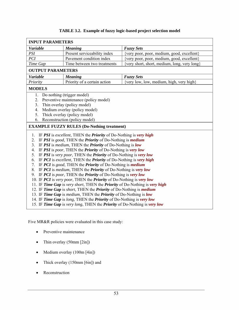
53

TABLE 3.2. Example of fuzzy logic-based project selection model

INPUT PARAMETERS Variable Meaning Fuzzy Sets PSI Present serviceability index {very poor, poor, medium, good, excellent} PCI Pavement condition index {very poor, poor, medium, good, excellent} Time Gap Time between two treatments {very short, short, medium, long, very long} OUTPUT PARAMETERS Variable Meaning Fuzzy Sets Priority Priority of a certain action {very low, low, medium, high, very high} MODELS

1. Do nothing (trigger model) 2. Preventive maintenance (policy model) 3. Thin overlay (policy model) 4. Medium overlay (policy model) 5. Thick overlay (policy model) 6. Reconstruction (policy model)

EXAMPLE FUZZY RULES (Do-Nothing treatment)

1. IF PSI is excellent, THEN the Priority of Do-Nothing is very high 2. IF PSI is good, THEN the Priority of Do-Nothing is medium 3. IF PSI is medium, THEN the Priority of Do-Nothing is low 4. IF PSI is poor, THEN the Priority of Do-Nothing is very low 5. IF PSI is very poor, THEN the Priority of Do-Nothing is very low 6. IF PCI is excellent, THEN the Priority of Do-Nothing is very high 7. IF PCI is good, THEN the Priority of Do-Nothing is medium 8. IF PCI is medium, THEN the Priority of Do-Nothing is very low 9. IF PCI is poor, THEN the Priority of Do-Nothing is very low 10. IF PCI is very poor, THEN the Priority of Do-Nothing is very low 11. IF Time Gap is very short, THEN the Priority of Do-Nothing is very high 12. IF Time Gap is short, THEN the Priority of Do-Nothing is medium 13. IF Time Gap is medium, THEN the Priority of Do-Nothing is low 14. IF Time Gap is long, THEN the Priority of Do-Nothing is very low 15. IF Time Gap is very long, THEN the Priority of Do-Nothing is very low

Five MR&R policies were evaluated in this case study:

• Preventive maintenance

• Thin overlay (50mm [2in])

• Medium overlay (100m [4in])

• Thick overlay (150mm [6in]) and

• Reconstruction

54

Six groups of fuzzy logic rules were developed – one for the do-nothing policy (trigger model)

and one for each of the five policies investigated. The case study only considered one treatment in each

policy. This is a simplification used only to illustrate the effectiveness of the approach and verify the

reasonableness of the algorithms.

The case study was run using a fifty-year analysis period and a discount rate of 4%. The MR&R

activities and their timing were determined by the fuzzy logic models. The agency costs were then

computed for each policy using the various treatment costs presented in Table 3.3. This table also

presents the effect of treatments on pavement condition variables PSI, PCI, and time gap. The salvage

values were considered proportional to the remaining service life (based on PSI) at the end of the analysis

period and the reconstruction cost. Pavement condition parameters were reset after a treatment in

accordance with the treatment effect indicated in Table 3.3.

TABLE 3.3. Cost and effect of the MR&R treatments considered

Treatment Effect Treatment Cost

(per lane-mile) PSI PCI Time Gap Preventive Maintenance $ 10,560.00 min(PSI+0.5, 4.5) min(PCI+20, 100) Reset to 0

Thin Overlay $ 37,875,20 4.5 100 Reset to 0 Medium Overlay $ 68,710.40 4.5 100 Reset to 0 Thick Overlay $ 99,575.60 4.5 100 Reset to 0 Reconstruction $ 218,552.92 4.5 100 Reset to 0

The present worth of the total life-cycle costs over the 50 years for the five policies evaluated is

presented in Table 3.4. Figures 3.5 and 3.6 present the priority progression with time for medium overlay

and reconstruction policies, respectively. The expenditure stream diagrams for the two policies are as

shown in Figures 3.7 an 3.8.

55

TABLE 3.4. Results obtained with the fuzzy logic-based LCCA model

Fuzzy Logic Based LCCA Result Policy Total Cost

(Present worth) Average PSI Average PCI

Preventive Maintenance $ 233,720.44 3.77 98.9 Thin Overlay $ 240,163.68 4.05 93.3 Medium Overlay $ 263,609.52 4.14 89.2 Thick Overlay $ 279,239.19 4.13 85.6 Reconstruction $ 258,110,28 3.38 80.2

0.00

0.20

0.40

0.60

0.80

1.00

0 10 20 30 40 50

Time (years)

Prio

rity

Do Nothing Medium Overlay

FIGURE 3.5. Priority progression for the medium overlay policy.

0.00

0.20

0.40

0.60

0.80

1.00

0 10 20 30 40 50

Time (years)

Prio

rity

Do Nothing Reconstruction

FIGURE 3.6. Priority progression for the reconstruction policy.

56

-250

-200

-150

-100

-50

0

50

100

150

200

250

1 3 5 7 9 11 13 15 17 19 21 23 25 27 29 31 33 35 37 39 41 43 45 47 49 51

Time (years)

Exp

endi

ture

(Tho

usan

d $)

FIGURE 3.7. Expenditure stream for the medium overlay policy.

-250

-200

-150

-100

-50

0

50

100

150

200

250

1 3 5 7 9 11 13 15 17 19 21 23 25 27 29 31 33 35 37 39 41 43 45 47 49 51

Time (years)

Exp

endi

ture

(Tho

usan

d $)

FIGURE 3.8. Expenditure stream for the reconstruction policy.

The results show a reasonable tendency among different policies. The preventive maintenance

policy has the lowest LCC and results in the highest average PCI. However, the average PSI is the lowest

because of the low effect of this treatment on PSI, as shown in Table 3.3; preventive maintenance mainly

retards the deterioration progress. The three overlay policies result in similar and acceptable average PSI

and PCI throughout the analysis period. The total present worth of agency costs increases with the

thickness of overlay. This tendency indicates that a treatment applied earlier could save more money than

a thick overlay applied later, while providing a similar average serviceability level. The reconstruction

policy has the lowest average PSI and PCI values. While the policies studied represent only a

57

hypothetical and simplified version of those generally considered by most highway agencies, the results

are very promising and suggests the feasibility of the approach.

DISCUSSION

Although the example presented in this paper helped establish the feasibility of the proposed approach,

there are still many possible enhancements to the model. For example, soft computing-based multi-

attribute decision support algorithms may facilitate the incorporation of non-monetary factors (e.g.,

environmental impacts and sustainability) into the engineering economic analysis process. This could be

a step towards the development of reliable procedures for long-term LCCA and BCA (i.e., 100 years and

more). Soft-computing based models for predicting pavement performance may also further enhance the

capabilities of the model. Furthermore, although the algorithms in this paper were developed for the

LCCA of pavements, they have been designed considering future expansion for their use with other

infrastructure assets. The use of consistent LCCA procedures for different kinds of transportation assets

(e.g., pavements, bridges, signs, and tunnels) is expected to facilitate the holistic integration of the

decision-making process for asset management.

CONCLUSION

Life cycle cost analysis (LCCA) is a key component in the pavement management process. LCCA is used

extensively to support project level decisions, and it has started to be used as a network level analysis

tool. Since LCCA is often based upon uncertain, ambiguous, subjective, and sometimes incomplete

information, soft computing techniques are particularly appropriate. Fuzzy logic systems provide a

formal approach for the treatment of these types of information. The feasibility and practicality of using

soft computing for developing LCCA tools was illustrated with the formulation and testing of a fuzzy

logic-based algorithm. Planned enhancements for the LCCA model include the incorporation of user

costs and the potential use of other soft computing techniques for performance modeling and for

incorporating non-monetary variable into the analysis process. The algorithm has the capability to be

expanded to handle other types of infrastructure assets.

58

REFERENCES

American Association of State Highway and Transportation Officials, (1993), Guide for Design of

Pavement Structures, AASHTO.

American Society of Civil Engineers, (2003), The 2001 Report Card for America’s Infrastructure.

http://www.asce.org/reportcard/, ASCE, accessed January 22, 2003.

Federal Highway Administration, (1998), Life-Cycle Cost Analysis in Pavement Design – Interim

Technical Bulletin, FHWA, Washington, DC.

Federal Highway Administration, (1999), Asset Management Primer. Office of Asset Management,

FHWA, Washington, DC.

Federal Highway Administration, (2002), Life Cycle Cost Analysis Primer. Office of Asset Management,


Federal Highway Administration, (2003), Economic Analysis Primer. Office of Asset Management,


Flintsch, G. W., (2002), Soft Computing Applications in Transportation Infrastructure Asset

Management. Application of Advanced Technologies in Transportation 2002, ASCE, August 2002.

Flintsch, G.W., (2003a) Soft Computing Applications in Pavement and Infrastructure Management: State-

of-the-Art. 82nd Transportation Research Board Annual Meeting, Washington, DC, 2003.

Flintsch, G.W., (2003b), Pavement Management Enhancement Using Soft Computing. MAIREPAV03 -

Third International Symposium on Maintenance and Rehabilitation of Pavements and Technological

Control, Guimarães, Portugal, 2003.

Furuta, H., Kanamori, A. and Dogaki, M., (1998), Optimal maintenance for RC decks of bridge network

based upon life cycle cost. Journal of the society of materials science, Japan, 47(12), 1245-1250.,

1998.

General Accounting Office, (2000), U.S. Infrastructure, Funding Trends and opportunities to Improve

Investment Decisions. Report to the Congress GAO/RCE/AIMD-00-35. General Accounting Office,

Washington, DC, 2000.

59

Jackson, N., and Mahoney, J., (1990), Washington State Pavement Management System, Federal

Highway Administration. Text for Advanced Course on Pavement Management, Nov. 1990.

Kerali, H., (1999), HDM-4 Highway Design & Management, Overview, Pre-Release. The Highway

Development and Management Series: The World Road Association (PIARC), 1999.

Kirk, S. J. and Dell'Isola, A. J, (1995), Life Cycle Costing for Design Professionals. McGraw-Hill, New

York, 1995.

Memmott, J. L., Richter, M., Castano-Pardo, A., and Widenthal, A., (1999) MicroBENCOST User

Manual Prepared for NCHRP project 7-12 (2): Metrification and enhancement of MicroBENCOST

software package. Transportation Research Board, NAS-NRC, Washington, DC, 1999.

National Cooperative Highway Research Program, (2001), Development and Demonstration of

StratBENCOST Procedure. Research Result Digest no 252, Summary of NCHRP 2-18 (3) and 2-18

(4), Transportation Research Board, NAS-NRC, Washington, DC, 2001.

Nauck, D., Klawonn, F., and Kruse, R., (1997), Foundations of neuro-fuzzy systems. John Wiley & Sons.,

1997.

Organization for Economic Cooperation and Development, (2001), Asset Management for the Roads

Sector. OECD, Paris, 2001.

Pappagiannakis, T. and Delwar, M., (2001), Computer Model for Life-Cycle Cost Analysis of Roadway

Pavements. Journal of Computing in Civil Engineering, Vol. 15, No. 2, 2001, pp. 152-156.

Usher, J.S. and Whifield, G.M., (1993), Evaluation of used-system life cycle costs using fuzzy set theory.

IIE Transactions, 25(6), 84-88., 1993.

Virginia Department of Transportation, (2002), Life Cycle Cost Analysis Pavement Options, Virginia

Department of Transportation, Materials Division/ Virginia Transportation Research Council, May

2002, 22 pp.

Walls, J., III and Smith, M. R., (1998), Life-Cycle Cost Analysis in Pavement Design. Technical Bulletin,

FHWA-98-079, Federal Highway Administration, Washington, DC, 1998.

60

Zadeh, L. A., (1973), Outline of a New Approach to the Analysis of Complex Systems and Decision

Processes. IEEE Transactions on Systems, Man and Cybernetics, SMC 3, 1973, pp. 28-44.

Zadeh, L. A., (1997), The Role of Fuzzy Logic and Soft Computing in the Conception, Design, and

Deployment of Intelligent Systems. In Software Agents and Soft Computing, Springer, 1997, pp.

183-190.

Zadeh, L. A., (2001), Apply Soft Computing – Foreword. Applied Soft Computing, Elsevier, 1(1), pp. 1-2.

61

CHAPTER 4: FUZZY LOGIC PAVEMENT MAINTENANCE AND REHABILITATION TRIGGERING APPROACH FOR PROBABILISTIC

LIFE-CYCLE COST ANALYSIS

Scheduled for publication in the Journal of Transportation Research Board in 2007.

TRB Paper Number: 07-2979

62

Fuzzy Logic Pavement Maintenance and Rehabilitation Triggering Approach for Probabilistic Life-Cycle Cost Analysis

By

Chen Chen1 and Gerardo W. Flintsch2

ABSTRACT: Life-cycle cost analysis (LCCA) is an important tool in the transportation Asset

Management process. Transportation agencies have used both deterministic and probabilistic LCCA

approaches. Probabilistic approaches allow decision makers to evaluate the risk of an investment

utilizing uncertain input variables, assumptions, or estimates. This paper explores the incorporation of

fuzzy-logic-based models into the risk analysis process to further enhance the traditional probabilistic

LCCA method. It proposes a fuzzy logic approach for determining the timing of pavement maintenance,

rehabilitation and reconstruction (MR&R) treatments in a probabilistic LCCA model for selecting

pavement MR&R strategies. Instead of using predefined service life for initial construction and future

rehabilitations, the proposed approach uses performance curves and fuzzy-logic triggering models to

determine the most effective timing of MR&R activities. The paper also compares this new approach to

the deterministic and traditional probabilistic approaches in a simple case study. The case study

demonstrates that the fuzzy-logic-based risk analysis model for LCCA can effectively produce results that

are at least comparable to those of the benchmark methods while effectively considering some of the

uncertainty inherent to the process.

1 Pavement Management Engineer, Asset Management Division, Virginia Department of Transportation, 1401

East Broad Street, Richmond, VA 23219, voice: (804) 662-9802, email: [email protected]

2 Associate Professor, The Via Department of Civil and Environmental Engineering; Director, Center for Safe

and Sustainable Infrastructure, Virginia Tech Transportation Institute, 3500 Transportation Research Plaza,

Virginia Polytechnic Institute and State University, Blacksburg, VA 24061-0105, voice: (540) 231-9748,

fax: (540) 231-7532, email: [email protected]

63

INTRODUCTION

Economic analysis is a critical component of today’s transportation Asset Management [1, 2].

Transportation Asset Management combines engineering principles and economic theory to facilitate a

more organized, logical approach to decision making [3]. Valuing the costs and impacts of highway

projects is an effective way to assess project-level alternatives, network-level plans, and strategic-level

policies. At the state-of-the-art level, the concept of economic analysis has been applied to every aspect

of the transportation Asset Management framework.

Life-cycle cost analysis (LCCA) is an important economic analysis tool in highway project

decision making. The concept of LCCA was originally developed by the U.S. Department of Defense in

the early 1960s to increase the effectiveness of government procurement. Since then, the concept of

LCCA has spread from defense-related issues to a variety of areas. From the very beginning, LCCA has

been closely related to design and development because it allows costs to be eliminated before they are

incurred as opposed to cutting costs afterward [4]. A common characteristic shared by most projects to

which LCCA is applied is that the studied systems are dynamic, which means their properties evolve over

time and change with their environments. This characteristic introduces a variety of uncertainties and risk

assessment requirements into the LCCA process.

The main purpose of LCCA in transportation is to support decisions in the planning, design, and

operation of major transportation projects. FHWA policy recommends LCCA as a decision support tool,

emphasizing that the results are not decisions in and of themselves. Often, the logical-analytical

framework implied in such analyses is as important as the LCCA results themselves [5].

The progress toward transportation Asset Management requires efficient economic analysis tools

to help state highway agencies with investment decisions. However, transportation agencies tend to avoid

LCCA and other economic analysis tools or hesitate to use their results as a reliable source to support

their decisions because:

64

1. The parameters and variables used in economic analysis are always uncertain and often

produce results that are also uncertain and possibly hard to interpret.

2. Agencies have the impression that economic analysis requires a lot of effort to determine

input values, run scenario iterations, and generate final results.

3. The scenarios recommended by the economic analysis tools may conflict with some of the

practices of the transportation agencies.

Some of these problems are due to misunderstanding of today’s economic analysis. For example,

economic analysis does not require significantly more information once the appropriate engineering

details are obtained. The level of effort required should reflect project costs, complexity, and possible

controversy over the evaluated project.

The traditional economic analysis approaches have some limitations. For LCCA, deterministic

methods cannot access the inherent uncertainty surrounding the input variables of economic analysis.

Thus this approach often ignores information that could improve the decision. A limited sensitivity

analysis may be conducted with various combinations of inputs, but it still often conceals uncertainty that

may be crucial to the decision-making process and may lead to debate over the validity of the results.

20 25 30 35 400

0.1

0.2

0.3

0.4

0.5

0.6

0.7

0.8

0.9

1(a)

Present Value ($ Millions)

Rel

ativ

e P

roba

bilit

y

Alternative AAlternative B

20 25 30 35 400

0.1

0.2

0.3

0.4

0.5

0.6

0.7

0.8

0.9

1(b)

Present Value ($ Millions)

Rel

ativ

e P

roba

bilit

y


FIGURE 4.1. Probabilistic LCCA result example

65

The probabilistic LCCA approach considers the random uncertainty in the LCCA process.

However, in many cases, the decisions based on understanding of the risks associated with different

alternatives are not straightforward. Figure 4.1 shows examples of the risk analysis results of an LCCA.

In Figure 4.1(a) alternative A has higher total life-cycle costs but a smaller variance than alternative B.

Since lower costs are preferred under normal situations, alternative B would be selected with an

acceptable risk (the shade area). However, LCCA may predict a larger variability (uncertainty) in the

results, as in Figure 4.1(b). If the decision maker prefers smaller risk, alternative A would be selected,

even if the mean life-cycle costs of the alternatives are same with the example in Figure 4.1(a).

While the probabilistic approach is more powerful than the deterministic one in terms of

uncertainty evaluation, it cannot handle all the sources of variability inherent in LCCA. Because the

information about initial construction is more complete and reliable, the majority of uncertainty in

economic analysis comes from future activities. Properly scheduling future activities in economic

analysis is a prerequisite for accurately estimating risks; this paper proposes a fuzzy logic solution to this

problem.

OBJECTIVE

This paper explores the incorporation of fuzzy-logic-based models into the risk analysis process for

selecting pavement maintenance, rehabilitation and reconstruction (MR&R) strategies using LCCA.

Instead of using predefined service life for initial construction and future rehabilitations, this research

used performance models coupled with a fuzzy-logic-based decision model to determine the timing of

MR&R activities. The prototype fuzzy-logic-based LCCA model was proposed by Chen et al. [6]. This

paper compares this approach with the traditional threshold trigger model used in the deterministic and

probabilistic LCCA methods. The practicality of the approach is illustrated with a simple case study.

66

LIFE-CYCLE COST ANALYSIS

The framework of LCCA approach includes five sequential steps [7]:

1. Establish design alternatives.

2. Determine activity timing.

3. Estimate costs (agency and user).

4. Compute life-cycle costs.

5. Analyze the results.

In terms of uncertainty consideration, there are two traditional LCCA approaches: deterministic

and probabilistic (risk analysis). Deterministic methods are simpler and easier to implement, but they do

not assess any risk that might be incurred. Probabilistic methods can account for the uncertainty in

variables, parameters, and results. Both methods require rehabilitation timings and costs as input

variables to their models.

Common Assumptions

Before any analysis can take place, several basic assumptions are needed, such as the same-benefit

assumption, analysis period length, and inclusion or exclusion of user costs. These issues directly affect

the reliability of final results. For example, if the same-benefit assumption does not hold, LCCA method

should not be used in the selection process. Other methods, like benefit-cost analysis, are more

appropriate in such conditions. Furthermore, if the selected period length is shorter than the design

service life of an alternative’s initial design, the results of LCCA would not be sufficient to reflect the

performance difference among different alternatives. Inclusion or exclusion of user costs is another

critical question faced by analysts in LCCA. While including user costs can make the final decision

making more justified, the credibility of available user-cost models is still disputed. The difficulty of

quantifying user-cost data discourages transportation agencies from considering this portion of costs.

67

Deterministic LCCA

In the deterministic LCCA method, all input variables and parameters are assumed to be known and are

assigned single, fixed values. The basic formula, as shown in Equation (1), calculates the present value

(PV) of costs over a facility’s life cycle.

1

1Initial_Cost Rehab_Cost(1 ) k

N

k nk

PVi=

⎡ ⎤= + ⎢ ⎥+⎣ ⎦

∑ (1)

where:

PV = present value of life-cycle costs,

Initial_Cost = initial construction costs,

Rehab_Cost = rehabilitation costs,

i = discount rate,

n = year of expenditure, and

k = rehabilitation number.

Interpretation of deterministic LCCA results is simple and straightforward. The alternative with

lowest expected life-cycle costs is favored. However, deterministic LCCA does not evaluate any

uncertainties. This limitation may lead to debates over the final results.

Probabilistic LCCA

The uncertainty in engineering economic analysis has been partially addressed by adopting probabilistic

methods and simulation techniques. Probabilistic LCCA methods allow the model to consider the

variability associated with input parameters over the life cycle of a project. Each input variable is

associated with a probability density function (PDF). Then, a simulation model is run for a certain

number of iterations or until some criteria are met. The statistical characteristics of output results, such as

mean and variance, represent the risk associated with future outcomes. A variety of computer-based tools

can realize such functions. Probabilistic LCCA assesses three basic questions about risk [5]:

1. What can happen?

2. What is the likelihood of it happening?

68

3. What are the consequences of it happening?

The computational capability of today’s computers has made possible the use of simulation for

risk analysis. Monte Carlo simulation is widely used in risk analysis. The statistical characteristics of

output variables can be captured with sufficient accuracy by running the simulation thousands or even

tens of thousands of times. For probabilistic LCCA, the final outputs would be the full range of possible

life-cycle costs and the relative probability of any particular total cost actually occurring.

The interpretation of probabilistic LCCA results goes beyond a simple comparison of the

alternatives’ mean life-cycle costs. The risks associated with each alternative are also important in

decision making. Alternatives with lower mean cost but higher risk would be difficult to compare to

those with higher mean cost but lower risk if the difference of mean values is not significant, as is the

case in Figure 4.1(b). Selection of an alternative would thus depend on the decision makers’ tolerance to

risk. Such judgments require reliable estimations of risk associated with alternatives. Otherwise, the

analysis will lead decision makers to an erroneous understanding of the risks associated with the

alternatives and thus compromise the efficiency of the decisions.

Therefore, the decision can be better supported when final outputs approach the realities. As

previously mentioned, both overestimated and underestimated risks may lead to sub-efficient decisions.

Since the variances of final outputs are determined by both input variables and internal inference

mechanics and since the quality of input information is generally given, increasing the accuracy of results

by improving the model’s internal inference mechanics is more realistic than improving data qualities.

UNCERTAINTIES IN LCCA INPUTS

Equation (1) describes the fundamental concept behind LCCA calculation: discounting all the costs

associated with the facility over its life cycle and summing them up. The variables in the equation

include initial construction costs, future rehabilitation costs, rehabilitation timing, and discount rate.

Figure 4.2 shows that these variables, except for discount rate, depend on more elementary items and are

69

often interrelated. For simplicity, the policies considered in this paper use only one type of maintenance

and rehabilitation treatment per alternative, but the treatment can be applied more than once. This

assumption simplifies the decision-making task to a to-do or not-to-do choice in the asset’s life cycle,

which eliminates the needs to first select proper type of rehabilitation and then determine the optimal

timing. The simplification is acceptable because the objective of LCCA is to investigate the relative

advantage between alternatives. As long as the model treats different alternatives in the same manner, the

results will not be affected. Many examples of such simplification can be found in the literature [5, 7].

Preliminary Engineering

Preliminary Engineering

Environ. Effects

Environ. Effects

Current Traffic

Current Traffic

Pavement Performance

Pavement Performance

Routine Maintenance

Routine Maintenance

Rehab. CostsRehab. CostsConstruction Management

Construction Management

Discount Rate

Discount RateGrowth RateGrowth Rate

Material Costs

Material Costs

Future Traffic

Future Traffic

Agency Policies

Agency Policies

Rehab. Timing

Rehab. Timing

Initial CostsInitial Costs

FIGURE 4.2. Relationship map of LCCA input variables and parameters

This section discusses the uncertainties in the four variables of the general LCCA model: discount

rate, initial construction costs, rehabilitation costs, and rehabilitation timing. Although the uncertainties

and their relationships can be analytically studied, the mathematical formulations will be significantly

cumbersome. This is one major reason why it is more practical to conduct a computer simulation as

previously discussed.

70

Discount Rate

As shown in Figure 4.2, discount rate is a stand-alone variable within the framework of LCCA. LCCA

has two options for discount rates: real or nominal. Real discount rates reflect the true monetary

opportunity value of time with no inflation components while nominal discount rates consider inflation

components as part of discounting concerns. In public transportation agencies, real discount rates should

be used because public sector project benefits should be dependent only on real gains (costing savings or

expanded output) rather than purely price effects [7].

A technical FHWA bulletin recommends a range of 3 to 5% as typical values for real discount

rates [5]. A symmetrical triangular distribution with a minimum, most likely, and maximum of 3, 4, and

5%, respectively, was used in this study.

Initial Construction Costs

An alternative’s initial construction costs pertain to putting the asset into initial service. Data on

construction are usually obtained from historical records, current bids, and engineering judgment. Since

nearly every alternative is more or less different from other alternatives, appropriate calculation and

deduction is necessary to obtain good estimations. According to Figure 4.2, the factors affecting the

estimation of initial construction costs include preliminary engineering (or engineering design), material

costs, and construction management. A simplified formula to estimate initial construction costs could be:

1

Initial_Costn

i ii

UC X=

= ⋅∑ (2)

where:

Initial_Cost = initial construction costs,

i = material type,

UCi = unit cost of material i, and

Xi = quantity of material i.

71

The quantity of each type of material is determined by engineering design and construction

management. In this research, the quantities and unit costs of materials for each pavement layer are

simulated using independent random variables. Using equation(2), the initial costs of alternatives are

calculated in each iteration of simulation. The quantity of materials (pavement layer thicknesses)

required by engineering design is also used in the performance prediction models.

Rehabilitation Costs

As a rule of thumb, rehabilitation activity needs to be applied to the asset at least once over its life cycle

to be able to capture long-term cost differences associated with reasonable design strategies. The purpose

of such activity is to maintain the asset above some predetermined condition, performance, and safety

level. With the assumption of single rehabilitation type, the costs of rehabilitation are related to the same

factors as initial construction costs: preliminary engineering, materials costs, and construction

management. The formula to estimate rehabilitation costs is shown in Equation 3:

1

Rehab_Costn

i ii

UC X=

= ⋅∑ (3)

Similar to the estimation of initial construction costs, the quantity and unit cost of materials are

simulated using independent random variables. The quantity of materials (layer thickness) of each

rehabilitation activity is incorporated with those of previous construction and rehabilitation activities to

predict the project’s performance.

The material quantity and unit cost variability of the rehabilitation treatments are considered to be

independent of each other. This is reasonable because it is unlikely that an agency would hire the same

contractor, use the same techniques, and manage the project with same level of quality on all activities. It

is more realistic to use independent random variables to simulate the activities rather than one random

variable for all rehabilitation events in the simulation.

72

Rehabilitation Timings

Traditionally, maintenance and rehabilitation in a project’s analysis period are determined using

predefined service life (SL). Some probabilistic LCCA methods consider a random variable for the SL of

initial construction and another independent random variable for all the rehabilitations [5]. A major

drawback of such a method is that rehabilitation activities are not likely to have same service lives. A

modified method uses a new independent random variable to predict the SL of each new rehabilitation

activity. However, this technique implies that the SLs of initial construction and rehabilitation are

independent of each other, which is apparently not true; the correlation between construction and

rehabilitation activities will be explained analytically in this section.

Rehabilitation costs are discounted using the present worth factor given by Equation (4):

1(1 )nPWF

i=

+ (4)

Thus, Equation (1) could be reformulated as Equation (5) by expanding the summation notation

and substituting the present worth factors of each activity into the equation:

1 1Initial_Cost Rehab_Cost Rehab_Cost N NPV PWF PWF= + × + + ×… (5)

Let PW_Rehabk denote Rehab_Costk kPWF× . Then Equation (5) becomes:

1Initial_Cost PW_Rehab PW_RehabNPV = + + +… (6)

Then the expected value of the final results of LCCA is:

1( ) (Initial_Cost) (PW_Rehab ) (PW_Rehab )NE PV E E E= + + +… (7)

And the variance of the final results of LCCA is:

73

1

1 1

2 2

var( ) var(Initial_Cost) var(PW_Rehab ) var(PW_Rehab )

2corr(Initial_Cost,PW_Rehab ) var(Initial_Cost) var(PW_Rehab )

2corr(Initial_Cost,PW_Rehab ) var(Initial_Cost) var(PW_Rehab )

2corr(Initial_Cost

NPV = + + +

+

+

+

+

…

…

1 2 1 2

1 1

N-1 N-1

,PW_Rehab ) var(Initial_Cost) var(PW_Rehab )

2corr(PW_Rehab ,PW_Rehab ) var(PW_Rehab ) var(PW_Rehab )

2corr(PW_Rehab ,PW_Rehab ) var(PW_Rehab ) var(PW_Rehab )

2corr(PW_Rehab ,PW_Rehab ) var(PW_Rehab

N N

N N

N

+

+

+

+

+

…

…

) var(PW_Rehab )N

(8)

The impacts of correlation between construction and rehabilitation events are represented by the

correlation coefficient items in Equation (8). For example, if an agency invests more today, it is likely

that the rehabilitation costs will happen later in the future. This relationship implies negative correlation

between adjacent events in LCCA. Therefore, if the correlation is properly considered, the variance of

final results should be reduced and could provide decision makers better supporting information.

As depicted in Figure 4.2, rehabilitation timing is the variable with the most explanatory factors

among the four inputs of LCCA models. It is determined by the studied project’s performance and the

rehabilitation policy, which determines the conditions under which the rehabilitation activity is applied.

The project’s performance can be predicted based on the engineering design, traffic load, and routine

maintenance level. Rehabilitation policies or strategies should be extracted from the agency’s previous

practices and knowledge. These practices can be simulated in LCCA by using either fuzzy logic

models—as proposed in this research—or threshold trigger models.

Potential Error Sources in Probabilistic LCCA

The primary source of error in simulation modeling is failure to recognize the dependent relationship

between input variables and parameters [5]. For accurate risk estimation, every iteration of a risk analysis

simulation must be of a scenario that can actually occur. For example, as shown in Figure 4.2, traffic and

pavement performance are correlated. The number of Equivalent Single-Axle Loads (ESALs) can be

used for traffic measurement and SL for pavement performance. For the same pavement structure,

74

greater ESALs will result in shorter SLs. Therefore, if the sampling mechanics for the two variables are

independent, unrealistic scenarios with high SL and high ESAL could occur in the simulation.

One way to consider the relationship among the variables is by using a correlation matrix in the

random sampling process. However, it would be very time and energy consuming to obtain the matrix

analytically. Most available pavement LCCA tools leave such tasks to the user. But if reliable

performance models are available, it is possible to incorporate them with decision models to predict

rehabilitation timing. The performance-based method implicitly considers the correlation between

rehabilitation events, as shown in Equation (8), and thus could estimate the variance of LCCA results

more accurately.

FUZZY-LOGIC-BASED LCCA ALGORITHM

Fuzzy logic systems were developed to provide soft algorithms for data processing that can make

inferences based on imprecise data. There are several characteristics of transportation asset LCCA that

make it particularly appropriate for using fuzzy logic techniques [8]. For example, the decisions about

rehabilitation level and timing are usually based on linguistic information like “good condition” or “poor

condition,” which is perfectly compatible with the inference pattern of fuzzy logic systems. This section

will briefly introduce the mechanics of fuzzy logic systems and review the fuzzy-logic-based

rehabilitation scheduling algorithm proposed by Chen et al. [6].

Fuzzy Logic Systems

The fuzzy logic system is an extension of the traditional rule-based reasoning (expert systems) that

incorporates imprecise, qualitative data in the decision-making process by combining descriptive

linguistic rules through fuzzy logic [9]. A typical framework of fuzzy logic systems includes four parts:

input processors (fuzzifier), rule base, inference engine, and output processors (defuzzifier). The fuzzifier

and defuzzifier provide mapping between crisp values and fuzzy sets. The concept of fuzzy set is the

fundamental basis of fuzzy logic systems. A fuzzy set is a set whose members have an associated

membership function value between 0 and 1, while the traditional crisp sets allow its members to take

75

values of only 0 or 1. The rule base is where the knowledge of models is stored. The knowledge can be

provided by experts, extracted from collected data, or both. The inference engine determine how the rules

are triggered and processed to map input values into outputs [10].

Determination of Rehabilitation Timing

Fuzzy logic systems can process uncertain information efficiently and can often generate good solutions

even with incomplete or imprecise data. This feature has been used in this research to determine asset

rehabilitation timing based on agency policies and performance models. Figure 4.3(a) presents the fuzzy-

logic-based MR&R triggering algorithm [6]. The algorithm consists of two rule-based fuzzy logic

models, a trigger model, and a policy model. Rules for both models can be customized according to the

agency’s policies or expert opinions. The trigger model computes the priority of a do-nothing policy,

while the policy model is used to evaluate the priority of specific rehabilitation treatments. Figure 4.3(b)

presents an example of the priority surfaces of three strategies five years after the initial construction for a

particular pavement structure and traffic level.

In this research, the fuzzy-logic-based trigger and policy model use same definition of

membership functions of input and output variables. A group of distinct inference rules are defined for

each model in the form of IF-THEN statements such as:

IF PSI is excellent, THEN the Priority of Do-Nothing is very high.

A complete description of membership functions and rules could be found elsewhere in [6]. The

algorithm evaluates the priorities of do-nothing activity and rehabilitation treatment year by year. If the

priority of rehabilitation exceeds that of the do-nothing activity, the treatment schedule is set to the year,

and all pavement conditions are adjusted accordingly. Otherwise, only routine maintenance is applied,

and the pavement is deteriorated following predefined performance models. The process is repeated for

every year in the analysis period. Finally, a schedule of rehabilitation events is generated for every

iteration and then used to calculate present worth factors.

76

Deterioration Model

SC1SC1

FC1FC1

SC2SC2

……

Fuzzy Policy Model

Fuzzy TriggerModel

MR & RAction

StructureStructure

LoadLoad

EnvironmentEnvironment

……

ΔSC1ΔSC1

ΔFC1ΔFC1

ΔSC2ΔSC2

……

Yes

Life Cycle Co$t

Year = Year + 1

No

Year = Year + 1

(a)

0 1 2 3 4 5

020

4060

80100

0

0.2

0.40.6

0.8

1

PSI

Do-nothing Model

PCI

Prio

rity

0 1 2 3 4 5

020

4060

80100

00.2

0.4

0.6

0.81

PSI

Thin Overlay Model

PCI

Prio

rity

0 1 2 3 4 5

020

4060

80100

00.2

0.4

0.6

0.81

PSI

Thick Overlay Model

PCI

Prio

rity

(b)

FIGURE 4.3. (a) Fuzzy-logic MR&R triggering algorithm; (b) Solution surfaces produced by the fuzzy logic models

Alternative A Alternative B

Policy Model Thin Overlay Thick Overlay

Trigger Model Do-nothing Do-nothing

77

COMPARATIVE CASE STUDY

This section presents a case study to compare the three LCCA approaches: (1) deterministic approach

with threshold trigger decision models; (2) probabilistic approach with threshold trigger decision models;

and (3) probabilistic approach with fuzzy logic triggering models. The objective of this case study is to

compare two MR&R strategies on one flexible pavement segment: thin overlay and thick overlay.

The segment is a single-lane, one-direction, one-mile-long, twelve-foot-wide section. As shown

in Table 4.1, its pavement structure consists of a 50-mm (2-inch) hot-mix asphalt (HMA) wearing course;

a 125-mm (5-inch) HMA intermediate layer; a 225-mm (9-inch) base layer; and a 150-mm (6-inch)

cement-treated aggregate subbase layer. The subgrade modulus is 5,000 psi. The two rehabilitation

strategies, thin overlay (Alternative A) and thick overlay (Alternative B), are also summarized in the

table. The initial average daily traffic was 12,000 vehicles. The traffic loads have a growth rate of 6%

according to the traffic monitoring data on Interstate Highway I–81 from 1997 to 2002.

TABLE 4.1. Engineering Design Parameters for Alternatives A and B

Variable Alternative A (thin-overlay)

Alternative B (thick-overlay)

Initial Construction Surface Layer Thickness (in.) 2 inch Intermediate Layer Thickness (in.) 5 inch Base Layer Thick 9 inch Traffic growth rate (yearly) 6 inch Rehabilitation Mill Depth (in.) 1 inch 2 inch Surface Layer Thickness (in.) 2 inch 2 inch Intermediate Layer Thickness (in.) 0 inch 4 inch

Cost data from the Virginia Department of Transportation (VDOT) were used to estimate mean

construction and rehabilitation costs [11] shown in Table 4.2. While the uncertainty of user costs could

be reflected in a higher variance in the results using the presented models, to simplify the example, user

costs were not considered in the case study. The analysis period in this study is selected as 50 years,

which is sufficient to reflect the performance difference of alternatives.

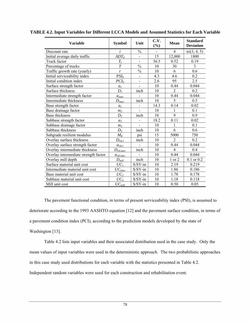
78

TABLE 4.2. Input Variables for Different LCCA Models and Assumed Statistics for Each Variable

Variable Symbol Unit C.V. (%) Mean Standard

Deviation Discount rate i % - 4 tri(3, 4, 5) Initial average daily traffic ADT0 - 15 12,000 1800 Truck factor Tf - 36.5 0.52 0.19 Percentage of trucks T % 10 30 3 Traffic growth rate (yearly) r % 10 6 0.6 Initial serviceability index PSI0 - 4.3 4.6 0.2 Initial condition index PCI0 - 2.6 95 2.5 Surface strength factor a1 - 10 0.44 0.044 Surface thickness D1 inch 10 2 0.2 Intermediate strength factor ainter - 10 0.44 0.044 Intermediate thickness Dinter inch 10 5 0.5 Base strength factor a2 - 14.3 0.14 0.02 Base drainage factor m2 - 10 1 0.1 Base thickness D2 inch 10 9 0.9 Subbase strength factor a3 - 18.2 0.11 0.02 Subbase drainage factor m3 - 10 1 0.1 Subbase thickness D3 inch 10 6 0.6 Subgrade resilient modulus MR psi 15 5000 750 Overlay surface thickness DOL1 inch 10 2 0.2 Overlay surface strength factor aOL1 - 10 0.44 0.044 Overlay intermediate thickness DOLinter inch 10 4 0.4 Overlay intermediate strength factor aOLinter - 10 0.44 0.044 Overlay mill depth Dmill inch 10 1 or 2 0.1 or 0.2 Surface material unit cost UC1 $/SY-in 10 2.19 0.219 Intermediate material unit cost UCinter $/SY-in 10 1.86 0.186 Base material unit cost UC2 $/SY-in 10 1.78 0.178 Subbase material unit cost UC3 $/SY-in 10 1.18 0.118 Mill unit cost UCmill $/SY-in 10 0.50 0.05

The pavement functional condition, in terms of present serviceability index (PSI), is assumed to

deteriorate according to the 1993 AASHTO equation [12] and the pavement surface condition, in terms of

a pavement condition index (PCI), according to the prediction models developed by the state of

Washington [13].

Table 4.2 lists input variables and their associated distribution used in the case study. Only the

mean values of input variables were used in the deterministic approach. The two probabilistic approaches

in this case study used distributions for each variable with the statistics presented in Table 4.2.

Independent random variables were used for each construction and rehabilitation event.

79

In the second approach, rehabilitation treatments were triggered at threshold performance

indexes. This was different from most of the state-of-the-practice methods used by many LCCA tools on

the market whose rehabilitation timing is determined by predefined service lives of initial construction or

rehabilitations. The fuzzy-logic-based model uses the fuzzy-logic MR&R triggering model and the same

pavement performance models to determine rehabilitation timings. Both simulation models were run for

1,000 iterations.

Distributions of Input Variables

According to the distribution determination method, input variables can be divided into two groups:

elementary variables and derived variables. Distribution of elementary variables can be obtained from

existing data or expert opinion. When existing data are available, such as bid price list and tested

structural capacity, both the distribution type and related controlling parameters need to be investigated.

The goodness-of-fit test is required to justify specific distributions. If no data exist, eliciting information

from expert opinion would be an effective way to set up distributions and evaluate the possible

interrelationships and codependencies among the input variables.

In this case study, truncated normal distributions were assumed for all variables to eliminate

unrealistic negative values. The only exception is with the discount rate, which was modeled using a

triangular distribution. The ranges of truncated normal distributions are the length of four standard

deviations. Therefore, for a symmetric distribution, its range is from two standard deviations less than the

mean value to two standard deviations greater than the mean value.

The coefficient of variations for the pavement performance parameters and other elementary

variables were obtained from Huang [14] when available. One exception is the initial serviceability

index. The 1993 AASHTO pavement design guide recommended using a value of 4.6 instead of the 4.2

used in the original 1986 guide based on a survey of the practices of the country [12]. Therefore, a

standard deviation of 0.2 is the maximum variance that could possibly have been considered in this study

80

to avoid an unrealistic PSI value larger than 5.0. Since there is no information available for the variances

of unit costs of materials, they were all assigned a coefficient of variation of 10% based on engineering

judgment.

Derived variables include initial construction costs, rehabilitation costs, rehabilitation timing, and

final total present worth. Their variances are all determined during the simulation. The initial

construction and rehabilitation costs are calculated using Equations (2) and (3), respectively. The total

present worth, which is actually the final output of LCCA, is calculated using Equation (1).

Performance Models and Decision Models

As previously mentioned, the AASHTO pavement design equation and pavement condition index

developed by the state of Washington were used to predict the pavement PSI and PCI, respectively. The

original AASHTO pavement design equation was rewritten to estimate PSI based on traffic loads,

structure number, and subgrade modulus as shown in Equations (9) and (10):

0tPSI PSI PSI= − Δ (9)

[ ]5.19

10940.4 log 9.36 log( 1) 0.2 2.32 log 8.07( 1)(4.2 1.5) 10

t RW SN MSNPSI

⎛ ⎞+ × − + + − +⎜ ⎟⎜ ⎟+⎝ ⎠Δ = − × (10)

where:

PSIt = predicted PSI at year t,

∆PSI = difference between the initial PSI and current PSI,

SN = structural number (adjusted after every rehabilitation according to overlay thicknesses),

Wt = cumulative ESALs applied to pavement from the last construction/rehabilitation, and

MR = subgrade modulus.

The reliability item was removed from the equation because the variability of the variables was

considered by directly assigning a distribution to them as shown in Table 4.2. The structure number of

pavement was adjusted according to the mill depth and overlay thicknesses every time a rehabilitation

activity was applied.

81

The following PCI models developed for Washington were used for the different types of

pavement [13]:

1. New flexible pavement:

2.00 0.22( )PCI PCI AGE= − (11)

2. AC overlay (1.2 inches to 2.4 inches):

1.750 0.76( )PCI PCI AGE= − (12)

3. AC overlay (over 2.4 inches):

1.750 0.54( )PCI PCI AGE= − (13)

After every rehabilitation activity, both PSI and PCI were reset to their new condition values,

which were randomly sampled from an independent distribution according to Table 4.2. Then, the

performance of pavement progressed according to the corresponding models.

The decision models proposed in this research are the fuzzy-logic-based models described in the

previous section. They are compared with traditional threshold trigger models used in deterministic and

probabilistic methods. For thin overlay policy (Alternative A), the thresholds values considered were 3.5

for PSI and 65 for PCI, whichever comes first; for thick overlay policy (Alternative B), they were 2.5 for

PSI and 45 for PCI, whichever comes first. These were adopted based on engineering judgment.

LCCA Results

The results of the deterministic LCCA method are summarized in Figure 4.4. Figure 4.5 presents the risk

analysis results using (a) the threshold trigger model and (b) the fuzzy-logic triggering model. As

expected, the mean values of the probabilistic model’s outputs are close to the results of the deterministic

model; the differences are due mostly to the random sampling of the simulation model.

82

0 10 20 30 40 50-300

-200

-100

0

100

200

300

Year

Cos

ts ($

1,00

0)

Expenditure stream diagram for Alternative A

0 10 20 30 40 50-300

-200

-100

0

100

200

300

Year

Cos

ts ($

1000

)

Expenditure stream diagram for Alternative B

PV = $281,600

PV = $311,800

FIGURE 4.4. Expenditure stream diagram for alternative A and B using deterministic method

Although the decision-making mechanics are different, the risk analysis results of the method

using fuzzy-logic-based models are also comparable with the results using threshold trigger models.

However, in fuzzy-logic-based models, a group of rules is defined according to the policy of

transportation agencies and activated by the inference engine to determine the rehabilitation timing. Such

mechanism allows the fuzzy-logic-based models to make decisions that mimic common human behavior

better than simple threshold trigger methods. The use of more elementary variables in the inference

process, such as layer thicknesses, also improves the credibility of final results.

83

200 250 300 350 4000

50

100

150

200

Present Value ($1000)

Freq

uenc

y

Alternative A

200 250 300 350 4000

50

100

150

200


Freq

uenc

y

Alternative B

200 250 300 350 4000

0.2

0.4

0.6

0.8

1


Cum

ulat

ive

Pro

babi

lity

Cumulative probability


(a)

200 250 300 350 4000

50

100

150

200Alternative A


Freq

uenc

y

200 250 300 350 4000

50

100

150

200Alternative B


Freq

uenc

y

200 250 300 350 4000

0.2

0.4

0.6

0.8

1Cumulative Probability


Cum

ulat

ive

Pro

babi

lity


(b)

FIGURE 4.5. Risk profile of PV for alternatives A and B using (a) threshold trigger model and (b) fuzzy-logic triggering model

Basic Statistic Alternative A Alternative BMean 286,540.00$ 321,720.00$ Std. Dev. 15,221.00$ 15,752.00$ C.V. 5.31% 4.90%

Basic Statistic Alternative A Alternative BMean 285,350.00$ 314,130.00$ Std. Dev. 15,973.00$ 15,987.00$ C.V. 5.60% 5.09%

84

It can be seen that the results of all three models favor Alternative A in the case study. This is

reasonable because thin-overlay treatments applied earlier are in general more economic than thicker-

overlays applied later. In the deterministic method, Alternative A is preferred because its PV of $297,530

is lower than that of Alternative B, $311,800. In the threshold-trigger-model-based probabilistic method,

Alternative A is preferred again because it has lower PV costs and similar variance. However, because

the cost distributions of the two alternatives have a large overlap, the risk of selecting B over A solely

based on lower PV costs is high. In the fuzzy-logic-based probabilistic method, the decision also favors

Alternative A in terms of lower PV costs and similar variance. One interesting finding is the fuzzy-logic-

based risk analysis gives a slightly lower variance than trigger-model-based risk analysis. This feature is

desirable in decision making because it increases the significance of alternative preference. However,

more extensive research is needed to draw a solid conclusion about it.

The results of the case study indicate that the statistical characteristics of output results could be

effectively captured in the risk analysis of fuzzy-logic-based LCCA algorithms. When rehabilitations are

triggered by performance and decision models, the correlations are implicit in the simulation; thus, they

accurately estimate the variance of final PV results.

Sensitivity Analysis

Figure 4.6 illustrates the probability of performing rehabilitation, via thin or thick overlay, at a particular

year for both models. The probabilities of rehabilitation timing using the threshold-trigger-model-based

probabilistic LCCA method concentrate more on several discrete years while the probability distribution

using fuzzy-logic-based decision models spread over a 4- or 5-year period flatly. This could be a sign

that if the results of the probabilistic LCCA approach are sensitive to the decision models, a small change

of threshold value in the traditional trigger decision model could cause a big difference in the final

decision. Considering threshold values as the only parameters in trigger decision models, a sensitivity

analysis was performed to evaluate the effects of PSI and PCI threshold values on final results. Its results

85

were compared with the findings by Chen and Flintsch [15] on the sensitivity analysis for fuzzy-logic-

based LCCA approaches.

0 10 20 30 40 500

100

200

300

400

500

600Alternative A

Year

Freq

uenc

y

0 10 20 30 40 500

100

200

300

400

500

600Alternative B

Year

Freq

uenc

y

(a)

0 10 20 30 40 500

100

200

300

400

500

600

Year

Freq

uenc

y

Alternative A

0 10 20 30 40 500

100

200

300

400

500

600

Year

Freq

uenc

y

Alternative B

(b)

FIGURE 4.6. Probability of rehabilitation timing using (a) threshold trigger model and (b) fuzzy-logic triggering model

The sensitivity analyses were implemented separately for Alternative A and Alternative B. The

variation ranges for PSI and PCI threshold were [3.0, 4.0] and [55, 75], respectively, for Alternative A

86

and [2.0, 3.0] and [35, 55], respectively, for Alternative B. The resulting correlation coefficients are as

shown in Table 4.3. It is significant that final PV results were highly correlated with the threshold values.

This relationship indicates that the quality of the decisions based on LCCA results of the probabilistic

approach using trigger models is greatly affected by the threshold values. If the threshold values are not

properly selected or cannot accurately represent the agency’s practices, decision makers may be misled by

the LCCA results.

TABLE 4.3. Correlation Sensitivity for Alternatives A and B

Alternative A (thin-overlay)

Alternative B (thick-overlay) Variable

Interval Mean Std. Dev. Interval Mean Std. Dev.

PSI Threshold [3.0, 4.0] 0.9130 0.8917 [2.0, 3.0] 0.9401 0.7824

PCI Threshold [55, 75] 0.9869 -0.3094 [35, 55] 0.9952 0.6722

With a similar case study, the research by Chen and Flintsch [15] found that as long as the system

structure could correctly capture the decision process practiced by an agency, the LCCA results and final

preference based on them were relatively stable when small changes were made on membership functions

of fuzzy logic systems. Compared to the finding in sensitivity analysis of trigger-model-based LCCA, the

stability of fuzzy-logic-based model is more desirable for transportation agencies in decision making

because a stable LCCA model means the decisions based on it will be consistent.

SUMMARY AND CONCLUSIONS

LCCA is a powerful economic analysis tool for supporting transportation Asset Management decision

making. It is used to support project-level decisions and to evaluate agency-level Asset Management

strategies. Fuzzy logic systems provide a formal approach for making inferences based on the uncertain,

ambiguous, and subjective information commonly available for LCCA. This paper proposes a fuzzy-

logic-based approach for determining the timing for pavement MR&R treatments in a probabilistic LCCA

model for selecting pavement MR&R strategies. This approach enhances the traditional probabilistic

87

LCCA method by adding the capability of processing some of the ambiguous uncertainty involved in the

decision process. The paper illustrates the feasibility of the proposed approach through a comparative

case study. The case study compared threshold trigger-based deterministic, threshold-trigger-based

probabilistic, and fuzzy-logic-based probabilistic approaches. The example demonstrated that the fuzzy-

logic-based risk analysis model for LCCA can effectively produce results that are at least comparable to

those of the benchmark methods, while allowing consideration of some of the ambiguous uncertainty

inherent to the process.

FUTURE ENHANCEMENT

While the research shows the feasibility and some potential advantages of fuzzy-logic-based probabilistic

method, further efforts are necessary to improve the methodology and promote its application in

pavement management practice. The following list discusses some of the possible improvements:

1. One advantage of fuzzy logic system is it can include linguistic information as well as

numerical information. Considering today’s pavement management practices rely on

engineering experience heavily while more and more numeric data are accumulated, fuzzy

logic techniques provide a unique solution to combine the two categories of information.

Mendel [10] indicated that using fuzzy basis functions (FBF) could produce strong coupling

between rules from knowledge mining and numeric data. The next phase of this research is

to tune the fuzzy logic models with real world data, such as the pavement conditions before

appropriate MR&R treatment.

2. Accurately capturing the probability distribution of input variables is a prerequisite of

efficient decision-support from probabilistic LCCA. Although normal distribution and

symmetric triangular distribution are popular choices in most cases, more accurate

distribution functions could be built based on real information. Defining more reliable

distribution functions would help produce results and risk evaluations closer to the actual

conditions.

88

REFERENCES

1. FHWA, Asset Management Primer, Office of Asset Management, Federal Highway

Administration, Washington, DC. 1999.

2. OECD, Asset Management for the Roads Sector, Organisation for Economic Co-Operation and

Development, OECD, Paris, France. 2001.

3. FHWA and AASHTO, Asset Management: Advancing the State of the Art Into the 21st Century

Through Public-Private Dialogue, Federal Highway Administration, Washington, DC. 1996.

4. Emblemsvag, J., Life-cycle Costing: Using Activity-based Costing and Monte Carlo Methods to

Manage Future Costs and Risks, John Wiley & Sons, New York. 2003.

5. FHWA, Life-Cycle Cost Analysis in Pavement Design - Interim Technical Bulletin, Federal

Highway Administration, Washington, DC. 1998.

6. Chen, C., G. W. Flintsch, and I. L. Al-Qadi. Fuzzy Logic-based Life-Cycle Costs Analysis model

for Pavement and Asset Management. in 6th International Conference on Managing Pavements,

Oct. 19-24, 2004. Brisbane, Australia. 2004

7. FHWA, Life-Cycle Cost Analysis Primer, Office of Asset Management, Federal Highway

Administration, Washington, DC. 2002.

8. Flintsch, G. W. and C. Chen, Soft computing applications in Infrastructure Management. Journal

of Infrastructure Systems, ASCE. 10(4), 2004, p. 157-166.

9. Zadeh, L. A. Outline of a new approach to the analysis of complex systems and decision

processes. in IEEE Transactions on Systems, Man and Cybernetics, SMC3 1973

10. Mendel, J. M., Uncertain Rule-Based Fuzzy Logic Systems: Introduction and New Directions,

Upper Saddle River, NJ, Prentice Hall. 2001.

11. VDOT, Life Cycle Cost Analysis Pavement Options, Materials Division/ Virginia Transportation

Research Council, Virginia Department of Transportation. 2002. p. 22.

89

12. AASHTO, Guide for Design of Pavement Structures, American Association of State Highway

and Transportation Officials, Washington DC. 1993.

13. Jackson, N. and J. Mahoney, Washington State Pavement Management System, in Text for

Advanced Course on Pavement Management, Federal Highway Administration. 1990.

14. Huang, Y. H., Pavement Analysis and Design, Upper Saddle River, NJ, Prentice Hall, Inc. 1993.

503-504.

15. Chen, C. and G. W. Flintsch. Sensitivity Analysis for Fuzzy-Logic-Based Life-cycle Cost Analysis

Approach. in 6th National Conference on Transportation Asset Management, Nov 1-3, 2004.

Kansas City, MO, USA. 2005

90

CHAPTER 5: CALIBRATING FUZZY-LOGIC-BASED PAVEMENT REHABILITATION DECISION MODELS USING THE LTPP DATABASE

91

Calibrating Fuzzy-Logic-based Pavement Rehabilitation Decision Models Using the LTPP Database

By

Chen Chen1 and Gerardo W. Flintsch2

ABSTRACT: This paper establishes a systematic method to calibrate a fuzzy-logic-based

pavement rehabilitation decision model using real cases extracted from the Long Term Pavement

Performance (LTPP) database. The fuzzy system was developed to conduct life cycle costs analysis

(LCCA) of transportation infrastructure assets. The following tasks had to be completed to develop the

proposed method: (1) extract representative rehabilitation events and related pavement information from

the database; (2) identify proper input areas for engineering knowledge and numeric data; and (3)

simultaneously tune two fuzzy logic systems with shared membership functions for input variables. A

total of eight tables in the LTPP database were used to extract pavement performance and rehabilitation

information. The investigation started with 62 rehabilitation cases but only six overlay rehabilitations

with thicknesses between 1.5 and 2.5 inches had all the required information and were thus selected to

calibrate the decision model. To make the dataset unbiased, six do-nothing cases were created based on

the rehabilitation cases. By reinterpreting the model in the form of neural fuzzy system, the calibration

algorithm was able to successfully tune the decision model to distinguish between the rehabilitation and

do-nothing cases.

1 Pavement Management Engineer, Asset Management Division, Virginia Department of Transportation, 1401

East Broad Street, Richmond, VA 23219, voice: (804) 662-9802, email: [email protected]

2 Associate Professor, The Via Department of Civil and Environmental Engineering; Director, Center for Safe

and Sustainable Infrastructure, Virginia Tech Transportation Institute, 3500 Transportation Research Plaza,

Virginia Polytechnic Institute and State University, Blacksburg, VA 24061-0105, voice: (540) 231-9748,

fax: (540) 231-7532, email: [email protected]

92

INTRODUCTION

Business decisions regarding pavement, bridges, and other infrastructure assets are made daily in the

operation of transportation agencies. Engineering management systems have been developed by local,

state, and national agencies to support these decisions. The process started with the development of

pavement management systems (Hudson et al., 1968), continued with bridge management systems

(Hudson et al., 1987) and infrastructure management systems (Hudson and Hudson, 1994), and has

recently evolved into asset management. The implementation of these systems allows transportation

agencies integrating massive data management, intensive computing capability, and sound engineering

experience from engineering and management staff to support their transportation infrastructure

investment decisions.

Transportation asset management decisions generally consist of two steps: (1) collecting quality

supporting information and (2) using the information, together with previous experience and knowledge

on the issue, to reach a decision. Modern engineering techniques such as automated data collection and

information technologies have made it possible for a transportation agency to obtain quality information

in an acceptable timeframe and at reasonable cost; however, the development of a sound knowledge base

still requires considerable time and tremendous efforts to achieve. The discovery of procedures and

approaches for effectively summarizing and extracting engineering knowledge from previous experience

is important for advancing transportation asset management.

Engineering economic analysis is a widely accepted technique to evaluate and measure the effectiveness

of decision options in transportation asset management (FHWA, 1999; OECD, 2001). Valuing the costs

and impacts of transportation projects in a monetary form is an objective way to assess project-level

alternatives, network-level plans, and strategic-level policies. Most economic analysis methods used in

transportation asset management, such as benefit cost analysis (BCA) and life cycle cost analysis

93

(LCCA), require the prediction of future project performance and future expenditures to control or correct

the deterioration of transportation infrastructures. Therefore, performance prediction models are critical

to support maintenance, rehabilitation and reconstruction (MR&R) decisions, which are based on the

progression of those dynamic properties (e.g., pavement roughness and cracking).

Infrastructure management MR&R decisions often consider many factors such as infrastructure design

and rehabilitation models, policies, availability of funding, and agency experience (FHWA, 1999). From

an engineer’s point of view, the most relevant factors are the infrastructure condition and treatment

effectiveness. The condition of a facility is usually determined by its structural and functional properties.

Studies to predict the condition of pavement, bridges, and other transportation assets are abundant in the

literature (Cattan and Mohammadi, 1997; Huang and Moore, 1997; Owusu-Ababia, 1998).

While asset performance models are abudant, efforts that summarize and consolidate real life decision-

making cases and experiences are rare in the transportation field. However, in practice project-level

decisions are often based on engineering judgment and experience. With first-hand management

experience and the best knowledge of their assets, engineers and asset managers are making decisions

everyday regarding pavements, bridges and other assets. Therefore, it would be appropriate to use an

agency’s specific experience to predict future MR&R activities in engineering economic analysis.

Utilizing the opinion and experience of the asset management staff should lead to realistic predictions.

OBJECTIVE

This paper establishes a systematic method for calibrating the fuzzy-logic-based rehabilitation decision

model proposed by Chen et al. (2004) using real cases extracted from the Long Term Pavement

Performance (LTPP) database. The steepest descent method and back-propagation learning algorithm

were used to tune the model. To achieve the objective, the following tasks had to be accomplished:

1. Extract reliable cases of overlay treatment from the LTPP database;

2. Identify proper input areas for engineering knowledge and numeric data;

94

3. Simultaneously tune two fuzzy logic systems with shared membership functions for input

variables.

FUZZY-LOGIC-BASED DECISION MODEL

The decision model to be calibrated in this research was first proposed by Chen et al. (2004) as a module

to schedule rehabilitation activities for LCCA. As shown in Figure 5.1, the decision model consists of

two fuzzy logic systems, namely, Fuzzy Trigger Model and Fuzzy Policy Model. Rules for both models

can be customized according to the agency’s policies or expert opinions. The trigger model computes the

priority of a do-nothing policy, and the policy model evaluates the priority of specific rehabilitation

treatments. The LCCA algorithm simulates the two mutually exclusive activities, do nothing and

rehabilitation, selects the most appropriate treatment for each year, and produces a rehabilitation schedule

for the analysis period. The algorithm compares the priorities computed by the two fuzzy logic models

each year, and the treatment with the highest priority is selected for that year.

Figure 5.1 shows that the algorithm’s prediction relies heavily on the deterioration model and the fuzzy-

logic-based decision model. With the help of modern mathematic techniques, including statistical

methods and adaptive modeling, the deterioration model could be established and calibrated to be used in

a specific geographic region with confidence. However, the studies of project-level decision models are

not abundant in today’s transportation asset management literature. An optimal, or adequate, decision

requires proper understanding of the properties of assets and the impacts of MR&R treatments. When

reliable history records are not available, the major, if not the only, source of information for constructing

the decision models is expert opinions and engineering experience. In this case, the decision-support

model can be initially developed based on the subjective experience. As objective data becomes

available, the decision models can be improved by calibrating these models with the accumulation of real

cases, which accurately reflect an agency’s MR&R practice. Therefore, a systematic approach is required

to incorporate existing expert knowledge and accumulated actual cases.

95

Deterioration Model

Distress(1)Distress(1)



……

Fuzzy Policy Model

Fuzzy TriggerModel

MR & RAction

YearYear

TrafficTraffic

StructureStructure

……

Δ Distress(1)Δ Distress(1)



……

Yes

Life Cycle Cost

Year = Year + 1

No

Year = Year + 1

FIGURE 5.1. Fuzzy-Logic-based Decision Model (Chen et al., 2004)

DATA PREPARATION

Ideally, if not enough historical information is available at the time of developing of the models, the

fuzzy-logic-based decision model can be initially designed mainly using expert knowledge and then

periodically reviewed and tuned as quality data accumulates. This approach was followed in this

research. The data used to tune the decision model were extracted from the LTPP database. The LTPP

program, initiated under the Strategic Highway Research Program (SHRP), has accumulated substantial

pavement condition information from in-service pavements throughout the United States and Canada.

The LTPP database is probably the largest pavement condition data source in the world available for

public access. This fact makes it an ideal data source for this research. Figure 5.2 summarizes the

procedure used for extracting the required data from the database. The main steps of this process are

elaborated following.

96

EXTRACT PAVEMENT DATA• Performance Condition• Rehabilitation Type• Rehabilitation Reason

EXTRACT PAVEMENT DATA• Performance Condition• Rehabilitation Type• Rehabilitation Reason

IDENTIFY GEOGRAPHICAL REGION• Virginia• and Vicinity Regions (DC, DE, MD, WV, NC)

IDENTIFY GEOGRAPHICAL REGION• Virginia• and Vicinity Regions (DC, DE, MD, WV, NC)

REMOVE DEFICIENT CASES• with Incomplete Pavement Condition• with rehabilitation for Non-Pavement Reason• with conflicted condition data (2 types)

REMOVE DEFICIENT CASES• with Incomplete Pavement Condition• with rehabilitation for Non-Pavement Reason• with conflicted condition data (2 types)

SELECT REHABILITATION TYPE• 2” Asphalt Overlay• and Overlay Thickness within 2 ± 0.5”

SELECT REHABILITATION TYPE• 2” Asphalt Overlay• and Overlay Thickness within 2 ± 0.5”

FIGURE 5.2. Procedure for Extracting Training Data from LTPP Database

Geographical Area of Interest

Since climate and environment have significant impacts on pavement performance and rehabilitation

effectiveness, it is inevitable that rehabilitation decisions are also affected by the factors. Therefore,

identifying a specific region from which to extract cases would be helpful to reduce the complexity of the

model. The state of Virginia is the area of interest in this research. However, to have enough data for the

calibration study, five neighboring Mid-Atlantic States (the District of Columbia, Delaware, Maryland,

West Virginia, and North Carolina) were also included in the queries.

Pavement Condition Indicators

Pavement condition is usually measured by the severity of the distresses preset in the surface. Three

types of distresses were considered in the research: alligator cracking, rutting, and roughness. Alligator

cracking generally occurs when the pavement has been reached its fatigue life because of repetitive axle

load application. Rutting is depressions occurring in the pavement’s wheel path as a result of traffic

loads. Wire-line rut indices were used in this research for rutting measurement because the method

usually obtains rutting values with a wider range compared with traditional straight-edge methods. The

97

two distresses have been widely accepted as important indicators of soundness of pavement structures.

Pavement roughness is a measure of the surface deviations that produce a response in the suspension

system of the vehicles traveling over the road. It is important because it is directly noticeable to the

traveling public. The decision model was calibrated based on the pavement conditions immediately

before a certain type of rehabilitation.

Rehabilitation Treatments

The prevailing type of rehabilitation in Virginia is 1.5-inch overlay after pretreatment of the existing

pavement. However, other states might have different practices. After reviewing the rehabilitation

records of sections in the LTPP database, overlays between 1.5 and 2.5 inches were categorized as one

rehabilitation type. This rehabilitation type was referred as thin overlay for this research. Usually, an

overlay with thickness in this range is selected to repair pavements that have not suffered severe losses in

structural capacity, at which point major rehabilitation or reconstruction has yet become necessary.

Deficient Records

Not all rehabilitation records were ready to be used to calibrate a decision model capable of reflecting the

intended practices. Three types of deficient records were removed from the dataset to be used in

calibration. The first group is those with some desired information missing, such as no roughness data

collected before rehabilitation. Then, rehabilitations incurred by reasons other than poor pavement

conditions are deleted because this research only focuses on decisions due to engineering considerations.

The records removed in a last step are those conflicting with their sections’ major trend. Typical

abnormalities are unexpected performance improvement without any documented rehabilitations.

Building Dataset for Calibration

Once the rehabilitation events have been identified, section information, rehabilitation type and data, and

pavement conditions were extracted from the database to build the dataset as shown in Figure 5.3. Sixty-

98

two cases were originally extracted. However, after the cleansing, a total of six cases, as listed in Table

5.1, were finally used to calibrate the fuzzy-logic-based decision model in this study.

EXPERIMENT_SECTION• Maintenance State• Pavement Type• Section ID

EXPERIMENT_SECTION• Maintenance State• Pavement Type• Section ID

LTPPLTPP

Administration (ADM)

MON_DIS_AC_REVMON_DIS_PADIAS_ACMON_DIS_PADIAS42_AC• Alligator Cracking

MON_DIS_AC_REVMON_DIS_PADIAS_ACMON_DIS_PADIAS42_AC• Alligator Cracking

Monitoring (MON)

RHB_IMP• Rehabilitation Type• Rehabilitation Date• Overlay Thickness

RHB_IMP• Rehabilitation Type• Rehabilitation Date• Overlay Thickness

Rehabilitation (RHB)

RHB_CAUSE_INFO• Rehabilitation Reason

RHB_CAUSE_INFO• Rehabilitation Reason

MON_T_PROF_INDEX_SECTION• Rutting (wire line)

MON_T_PROF_INDEX_SECTION• Rutting (wire line)

MON_PROFILE_MASTER• Roughness

MON_PROFILE_MASTER• Roughness

Section QuerySection Query

Rehabilitation QueryRehabilitation Query

Condition QueryCondition Query

FIGURE 5.3. Data Extracted from the LTPP Database

TABLE 5.1. Rehabilitation Cases

Alligator Cracking Rutting Roughness Overlay

Thickness Case # State ID

(%) (inches) (inches/mile) (inches) 1 MD 0505 18.42% 0.24 116.11 2.0 2 MD 0561 23.90% 0.39 70.96 2.5 3 VA 1002 6.15% 0.20 172.74 1.5 4 VA 1023 4.59% 0.63 121.14 1.5 5 VA 1417 3.71% 0.24 175.63 1.5 6 VA 1423 5.09% 0.28 137.36 1.5

One potential drawback of the dataset is that all of the cases lead to the decision of thin-overlay treatment

which might introduce bias to the calibrated model. The solution is to add cases that lead to do-nothing

decisions. However, it is not easy to directly find suitable cases from the LTPP database because what

99

the dataset needs are cases such that current pavement conditions lead to do-nothing, but any further

development of distress would lead to rehabilitation. Conceptually, the rehabilitation cases were used to

create do-nothing cases by reducing the current distresses by 15%. The percentage was selected based on

engineering judgment. Adding these do-nothing cases made the dataset balanced. As a result, only a very

small dataset was used; however, it was large enough to illustrate the practicality of the approach.

DESIGN OF FUZZY LOGIC SYSTEMS

Fuzzy logic systems are an extension of the traditional rule-based reasoning (expert systems) that

incorporate imprecise, qualitative data in the decision-making process by combining descriptive linguistic

rules through fuzzy logic (Zadeh, 1973). A typical fuzzy logic system consists of four components:

fuzzifier (input processor), rule base, inference engine, and defuzzifier (output processor). The fuzzifier

and defuzzifier provide mapping between crisp values and fuzzy sets. The concept of fuzzy sets provides

the basis of fuzzy logic systems. There have been many references that explain the concept (Lin and Lee,

1996; Mendel, 2001). A fuzzy set is a set whose members have an associated membership function value

between 0 and 1, while the traditional crisp sets only allow its members to take value of 0 or 1. The rule

base is where the knowledge of models is stored. The knowledge needed to build the rules can be

provided by experts, extracted from collected data, or both. A form of IF-THEN clauses is often used to

store the knowledge. The inference engine determines how the rules are triggered and processed to map

input values into outputs.

Each of the four components has multiple options in designing the architecture of a fuzzy logic system,

which create almost infinite possibilities. The fuzzifier could be either singleton or non-singleton. The

membership functions could be triangular, trapezoidal, or Gaussian, among others. Typical composition

methods (operations) include max-min, max-product, etc. Examples of defuzzifier schemes include

centroid, height, and modified height. For simplicity, the fuzzy logic systems studied in this research

were designed using singleton fuzzification, Gaussian membership functions, product implication and t-

100

norm operations, and height defuzzification. The following discussion will focus on this specific

architecture unless indicated otherwise.

Selecting the architecture for a fuzzy logic system is more or less arbitrary and relies heavily on the

previous knowledge of a specific configuration. When numerical training data are also available, the

design methods could be categorized into the following 3 groups:

1. Let the data determine the key parameters for the fuzzy sets of input and output variables and

then establish inference rules;

2. Pre-define fuzzy sets for input and output variables and use data to determine inference rules; and

3. Manually design the architecture and then use the data to optimize its parameters according to

performance measures.

The first two approaches are called “one-pass methods” (Mendel, 2001) because the training data are only

used once in the design of the fuzzy logic system. The third approach usually needs to visit the training

data many times to obtain the best possible performance and therefore is called a “multiple-pass

methods”. When available data are accurate and sufficient for designing fuzzy logic systems, the two

one-pass methods may suffice. However, if it is time-consuming to collect quality information, the third

design method provides a more practical solution because it allows fully relying on expert knowledge at

the beginning and fine-tuning the model as quality information becomes available. This paper uses the

multiple-pass method to optimize the parameters of fuzzy-logic-based decision models.

Membership Functions

Gaussian functions are used in this paper to define the membership of each element in a fuzzy set. So for

a single input value of x, its fuzzy membership is given in equation (1).

2

2

( )( ) exp

2

lk

lk

lk

F

F

F

x mxμ

σ

−= −

⎛ ⎞⎜ ⎟⎜ ⎟⎝ ⎠

i = 1, …, N (1)

101

Where lkF

m = the mean value of Gaussian function of the kth input in the lth rule;

lkF

σ = the standard deviation of Gaussian function of the kth input in the lth rule.

The number of membership function terms for a specific input or output variable depends on the previous

experience about how many categories are enough. The simplest configuration (used in this research) is

categorizing each pavement distress condition into two groups: good or poor. For example, the rutting

condition was defined by two membership functions, one for good rutting condition and one for poor. A

specific rutting value could partially belong to good and poor at the same time in fuzzy logic systems.

Inference Rules

The Rule-bases store the knowledge of fuzzy logic systems. To fully utilize available expert knowledge,

the proposed tuning method starts by defining inference rules. If a fuzzy logic system has p inputs x1, x2,

…, xp, one output y, and M inference rules, then the lth rule has the form:

1 1: IF is and and is , THEN is is ;l l l l

p pR x F x F y G l = 1, …, M

Where lkF is the membership function term of the kth input (k = 1, …, p) in the lth rule and lG is the

membership function term of the output.

Since the decision model has three distress conditions as inputs, at least eight inference rules are required

to fully cover all possible premise conditions. Table 5.2 gives the inference rules and initial mean values

of output membership functions of the two fuzzy logic systems utilized in this research. If all three

conditions are good, the do-nothing option is of the highest priority, 1, and the rehabilitation option is of

the lowest priority, 0. As the pavement conditions deteriorate, the priorities of do-nothing decrease while

those of rehabilitation increase. Finally, when all three conditions are poor, rehabilitation gains an

overwhelming priority, 1, over do-nothing, 0.

102

TABLE 5.2. Inference Rule Bases of the Decision Model

Rule Alligator Cracking Rutting Roughness Do-Nothing

Priority Rehabilitation

Priority Premise Consequences

1 Good Good Good 1 0 2 Poor Good Good 0.75 0.25 3 Good Poor Good 0.75 0.25 4 Good Good Poor 0.75 0.25 5 Poor Poor Good 0.25 0.75 6 Poor Good Poor 0.25 0.75 7 Good Poor Poor 0.25 0.75 8 Poor Poor Poor 0 1

The logic behind this rule base is valid from the engineering perspective; do nothing to pavements in

good condition and rehabilitate pavements in poor condition. However, the challenge is to find the

correct value for priorities in each rule and the parameters, mean values and standard deviations, of the

various membership functions to make the decision model consistent with previous practices. To achieve

this ultimate goal, it is necessary to have a systematic procedure to calibrate the model using real cases.

The multi-pass method to tune a single fuzzy logic system based on system feedback was selected. This

method uses fuzzy basis function as a bridge connecting rule-based fuzzy logic system and mathematic

programming techniques.

Fuzzy Basis Functions

The concept of fuzzy basis functions was first introduced by Wang and Mendel (1992). Their objective

was to develop a mathematical formula representing how a crisp input x is mapped into a crisp output y =

f (x) through fuzzy logic systems. Let l

y denote the mean value of output membership function in the lth

rule. The mapping formula was constructed as follows:

1

( ) ( )lM

lly f y φ

== = ∑x x l =1, …, M (2)

Where ( )lφ x is the fuzzy basis function which is given based on specific choices for fuzzifier,

membership functions, composition, implication, t-norm and defuzzifier. For the architecture used in this

study, the fuzzy basis function is:

103

1

1 1

( )( )

( )

lk

lk

p

kk F

l pM

kl k F

x

x

μφ

μ

=

= =

=∏

∑ ∏x (3)

Where ( )lk

kFxμ is the value of membership of the kth input (k = 1, …, p) in the lth rule (l = 1, …, M).

Equation (2) indicates that, for output membership functions, only their mean values have impacts on

final results; the standard deviations do not affect the outputs when using the height defuzzification

method. The concept of fuzzy basis functions is very useful because it provides a general form of

function approximation for fuzzy logic systems. More explanation about fuzzy basis functions can be

found elsewhere (Wang and Mendel, 1992).

Steepest Descent Method

Steepest descent methods are also known as gradient descent methods. These methods have been widely

applied for solving nonlinear programming problems, such as learning algorithms of neural network. To

find the optimal solution, i.e., the maximum or minimum of a cost function f (x), it starts from a pre-

selected initial position, 0P , and as many times as needed, moves from iP to 1iP+ along the direction of

steepest gradient, ( )if P−∇ . Selecting the initial position is critical to the convergence of the solution.

Poorly selected initial positions may cause extremely long converging time and even result in stopping at

a local optimal position. However, expert knowledge usually gives a start point close to the optimal. If

this is the case, the tuning process would be dramatically simplified and expedited.

Tuning Fuzzy Logic Systems

Based on the idea of steepest descent method, Mendel (2001) developed a method to tune the antecedent

and consequent parameters in fuzzy logic systems. This method was used as the basis of the calibration

algorithm used in the paper and is briefly explained in this section.

If N groups of paired input-output data are available to tune a fuzzy logic system and x denotes the inputs

and y for output, the cost function for the ith group can be defined as follows:

104

2( ) ( )

( )( )

2

i i

sif y

e−

=⎡ ⎤⎣ ⎦x

i = 1, …, N (4)

Following the principle of steepest descent methods, three equations were developed to minimize ( )ie (i =

1, …, N, l = 1, …, M and k = 1, …, p):

( ) ( ) ( )

( )

( )

2

( 1) ( ) ( ) ( ) ( )

( )( )

( )

l lk k

lk

l

lk

li i i

m s sF F

i

k F i

F

m i m i f y y i f

x m i

i

α

φσ

+ = − − −

−×

⎡ ⎤⎡ ⎤⎣ ⎦ ⎣ ⎦⎡ ⎤⎣ ⎦

x x

x (5)

( ) ( ) ( )( 1) ( ) ( ) ( )l

l l i i i

syy i y i f yα φ+ = − −⎡ ⎤⎣ ⎦x x (6)

( ) ( ) ( )

2( )

( )

3

( 1) ( ) ( ) ( ) ( )

( )( )

( )

l lk k

lk

l

lk

li i i

s sF F

i

k F i

F

i i f y y i f

x m i

i

σσ σ α

φσ

+ = − − −

−×

⎡ ⎤⎡ ⎤⎣ ⎦ ⎣ ⎦

⎡ ⎤⎣ ⎦

x x

x (7)

Becausel

y , lkF

m and lkF

σ are parameters associated with membership functions for physically

meaningful quantities, it is usually possible to obtain very good initial values for them. Choosing them

smartly will help this algorithm to converge much faster (Chu and Mendel, 1994). The learning

parameters, mα , yα and σα must also be chosen with some care. Frequently, the same value of α is

chosen for all three equations.

MODEL CALIBRATION

A challenge associated with the tuning of the decision model in Figure 5.1 is how to simultaneously

optimize the design of two fuzzy logic systems. Since they share the same input variables, it will be ideal

if they would share the definition of membership functions of each input variable. Using the same

language in the two fuzzy logic systems facilitates expert knowledge acquisition and makes the model

easier to understand and accept by decision makers. However, this also means one more objective and

105

several more constraints in the calibration phase, which usually makes the nonlinear programming

problem more difficult to solve.

Fortunately, shared membership functions also provide direct connections between the two systems.

With these connections, the competition among two fuzzy logic systems can be reinterpreted as an

integrated neural fuzzy system. As shown in Figure 5.4, a feed-forward multilayer network was

constructed to describe the decision model in terms of a neural fuzzy system. The membership functions

and inference rules connected by solid lines are components of the trigger model and those connected by

broken lines belong to the policy model.

0

1

0

1

0

1

0

1

0

1

0

1

0

1

0

1

0

1

0

1

0

1

0

1

0

1

0

1

0

1

0

1

…


Priority_TPriority_T

Priority_PPriority_P

∑+1

-1

0: Do Nothing;1: MR&R Treatment.

y⎧

= ⎨⎩

…

IF THENIF THEN

IF THENIF THEN


Distress(p)Distress(p)

…IF THENIF THEN

IF THENIF THEN

IF THENIF THEN

IF THENIF THEN…

IF THENIF THEN

IF THENIF THEN

0

1

0

1

0

1

0

1

……

FIGURE 5.4. Reinterpreting the Decision Model in the form of a Neural Fuzzy System

Under this network structure, the input nodes represent transportation infrastructure conditions; the

hidden layers consist of nodes functioning as membership functions, fuzzy logic rules, and comparison of

priorities; and the output layer represents final decisions. The detailed explanation of the layers is as

follows:

106

• Input: Input nodes represent current condition of transportation assets. They are measured by the

extent or magnitude of the distresses considered.

• Hidden Layer 1: Each single node in this layer performs one membership function for a certain

input variable, i.e., a distress type in this study. Therefore, links between layer 1 and input nodes

only occur when the nodes are designated to a specific distress type.

• Hidden Layer 2: This layer represents the inference rules designed for the two fuzzy logic

models. It is possible to have multiple inputs for nodes of this layer when the represented rule

has multiple antecedents.

• Hidden Layer 3: Nodes in this layer are essentially the membership functions for the output

variables, the priorities of do-nothing or rehabilitation. Together with layer 2, this layer functions

as the inference engine of the two fuzzy logic models.

• Hidden Layer 4: The layer combines the outputs from the fuzzy logic rules in each of the two

models. A defuzzification method has to be pre-specified in the initial design phase.

• Output: The output layer gives the final recommended treatment. It compares the two output

priorities and selects a winner, i.e., the treatment with the higher priority. Therefore, the weight

of link is 1 between output node and the priority of the policy model and -1 for the priority of the

trigger model.

The five-layer neural fuzzy system makes it possible to use neural network learning techniques for this

research. The following section will further explain the benefits from integrating fuzzy logic and neural

network for calibrating the decision-support model.

Neural Fuzzy System

It has been widely accepted that fuzzy logic and neural networks are complementary technologies. When

expert knowledge is the major source for constructing a fuzzy logic system, the design process is more or

107

less arbitrary. Once the system is constructed, it will be difficult to identify the part to tune according to

numeric training data. On the other side, neural networks are good at learning from historic data, but the

links and nodes in hidden layers are usually hard to assign meaningful roles in a model. Combining them

into one integrated system allows for combining their advantages and minimizing the drawbacks.

Several previous studies suggested that the complementary features and characteristics of fuzzy systems

and neural networks warrant their integration (Werbos, 1992; Bersini et al., 1993; Pedrycz, 1993). On the

neural network side, by combining it with a fuzzy system, the structure provides more transparency and

allows a possible interpretation of the links and nodes following the learning stage. On the fuzzy set side,

neural networks’ learning algorithms allow automatic tuning of the parameters that characterize the fuzzy

system. Therefore, neural networks can improve their transparency, while fuzzy systems can self-adapt.

One major advantage of using the concept of neural fuzzy systems in this research is that the learning

abilities from neural networks make fuzzy systems adaptive to the process of accumulating reliable

MR&R cases. The membership functions were fine-tuned using the training data. At the same time, the

model also provides human-understandable meaning to the feed-forward multilayer neural network in

which the nodes are often opaque to users (Lin and Lee, 1996). This feature makes it possible to use

expert knowledge in both initial design and final validation phases.

Calibrating the Decision-support Models

With the network-structured decision model in Figure 5.4, it is a natural choice to use a back-propagation

(BP) learning algorithm to do the calibration work. The concept of BP learning was one of the most

important developments in neural networks (Werbos, 1974; Rumelhart and Zipser, 1986). In the

algorithm, the error(s) at the output layer is propagated backward to adjust the connection weights of

preceding layers to minimize output errors. After a number of iterations, multilayer feed-forward

networks can be systematically optimized by this algorithm. The back-propagation algorithm is

employed in most neural network applications.

108

As shown in Figure 5.4, the proposed decision-support model of this research consists of two fuzzy logic

systems. The definitions of the membership functions for the individual input variables are shared by the

two models, but each rule of the two systems has its own output membership function. The reasons for

such design are the following: (1) using the same language for input variables provides extra convenience

to incorporate expert knowledge; but (2) more flexibility is desired for the output membership functions

to improve the tuning of the model.

To implement the back-propagation learning algorithm, an error function is required to measure the

deviation from target output values. Mathematically, the outputs are 0 for do-nothing or 1 for thin-

overlay in this research. Because the raw data from the LTPP database are assumed to be pavement

conditions at which thin overlay rehabilitations are properly and timely triggered, the priority from policy

model is desired to be slightly larger than the priority from trigger model. Similarly, for the do-nothing

cases, the pavement conditions are assumed to be just before thin-overlay rehabilitation is properly

triggered. Therefore, when pavement conditions are deteriorated to a level just severe enough for

triggering thin overlay rehabilitation, the priority from the policy model is desired to be slightly lower

than the priority from trigger model. In other words, for the pavement conditions used in calibration, the

outputs from two fuzzy logic systems expected to be very close but still capable differentiate do-nothing

cases from rehabilitation cases. Based on this consideration, the error function was formulated as:

( ) ( ) ( ) ( ) ( )( ) Priority Priorityi i i i ipolicy triggere d f= − − (8)

Where ( )id = the desired decision based on the ith pair of pavement conditions;

( )if = the decision by decision model based on the ith pair of pavement conditions;

( )Priority ipolicy = the priority of rehabilitation produced by policy model;

( )Priority itrigger = the priority of do-nothing produced by trigger model;

109

The errors calculated by equation (8) are for the entire neural fuzzy system. Following the principle of

back-propagation method, the error propagated to trigger model is ( )ie− ; the error propagated to policy

model is ( )ie . The calibration essentially becomes tuning the two fuzzy logic systems. The parameters to

be tuned in the decision model include 6 mean values and 6 standard deviations for input membership

functions shared by the two fuzzy logic systems, and 16 mean values for output membership functions

(their standard deviations do not influence final results). An epoch is defined as the collection of N

training cases. It is important to notice that each of the 28 parameters only need to be updated once using

equations (5), (6) and (7) based on the error from one case. The six mean values and six standard

deviations for the input variables have to be updated simultaneously for both fuzzy logic systems.

Otherwise, their updating is not synchronous with the mean values of output membership functions which

may make it hard, or impossible, for the model to converge.

A number of variations of the algorithm exist by preprocessing the training dataset differently and/or

using different convergence criteria. The training dataset was preprocessed in the way shown in Figure

5.5. A calibration dataset was constructed by increasing the pavement distresses of do-nothing cases by

5% and decreasing those of rehabilitation cases by 5%. The preprocessing means that the decision model

is subject to a stricter calibration dataset but still the target is to differentiate the original do-nothing cases

from rehabilitation cases. Since only six cases were used, the convergence criteria used in this research

was to run the calibration until the decisions regarding all cases could be accurately predicted. As shown

in Figure 5.6, a total of 72 epochs were sufficient to get the decision model to converge.

Table 5.3 gives the values of the parameters of the decision model before and after calibration. All values

are rounded to numbers that are easily understandable from an engineer’s perspective. The principles to

determine the initial values are simple. First, the mean values of membership functions for good and poor

conditions should cover the range of training set. Secondly, the standard deviations are roughly one third

to half of the ranges.

110

Distress 1

Distress 2

Case 1: Distress 1, 2, …

0.85

Case 2

Case 3

Case 4

Case 5Case N …

1

Real Cases for Overlay Treatment

Fuzzy Zone in Calibration

Populated Cases used in Calibration


Populated Cases used in Testing

Real Cases for Overlay Treatment

Fuzzy Zone in Calibration



Populated Cases used in Testing

FIGURE 5.5. Cases of Overlay Treatment

0 10 20 30 40 50 60 70 80 90 1000

1

2

3

4

5

Epochs

Num

ber o

f Cas

es w

ith M

ista

ken

Dec

isio

n

FIGURE 5.6. Number of cases with mistaken decisions decreasing through multi-pass calibration

111

TABLE 5.3. Fuzzy-Logic-based Decision Model

Initial Values Values after Tuning Variable Membership

Function m σ m σ Good 5% 10% 0% 11% Alligator

Cracking Poor 25% 10% 17% 18% Good 0.1 0.3 0.07 0.32 Rutting Poor 1 0.3 0.92 0.45 Good 50 50 50 50 Roughness Poor 200 50 200 50 Rule 1 1 - 0.88 - Rule 2 0.75 - 0.60 - Rule 3 0.75 - 0.77 - Rule 4 0.75 - 0.75 - Rule 5 0.25 - 0.30 - Rule 6 0.25 - 0.25 - Rule 7 0.25 - 0.25 -

Do-Nothing Priority

Rule 8 0 - 0.00 - Rule 1 0 - 0.12 - Rule 2 0.25 - 0.40 - Rule 3 0.25 - 0.23 - Rule 4 0.25 - 0.25 - Rule 5 0.75 - 0.70 - Rule 6 0.75 - 0.75 - Rule 7 0.75 - 0.75 -

Rehabilitation Priority

Rule 8 1 - 1.00 -

DISCUSSION

The procedures for data extraction, initial design, and model calibration proposed in this research can be

readily adopted by transportation agencies to develop their own regional decision-support models. The

region could be state, district(s), or county(s) where the rehabilitation activities are conducted under

consistent policies. Building such models would benefit a specific area’s asset management from at least

two aspects. First, the engineering economic analysis can more accurately evaluate the impacts of

alternatives to the area because the decision models are based on their actual practices. Second, besides

the application in engineering economic analysis, the results of model calibration could also be used to

compare the impacts on rehabilitation decisions of a single distress and/or a combination of several

distresses.

112

Data Preparation

Although data from six states were initially selected for consideration, finally only six cases from two

states (Virginia and Maryland) were identified as adequate to be used in this research. There were 62

rehabilitation events recorded in the database. Most of them were deleted due to incomplete information.

The LTPP program requires pavement conditions data to be collected before and after any rehabilitation

events (Elkins et al., 2005). Participating agencies are requested to notify the LTPP regional office for

anticipated rehabilitation events. However, the LTPP database does not contain complete data for all

rehabilitation events. Although not in the database, it is reasonable to expect that most of the missing

information could be located somewhere in the responsible transportation agency because, usually,

rehabilitation is applied to address the issues that have been discovered. When similar research is

conducted to investigate the decision behaviors of an agency, it is recommended to exhaust all possible

sources before excluding a rehabilitation case. Useful complementary information might be found in

pavement condition reports, project proposals, and/or district records. The pool of rehabilitation events

would be significantly enlarged if the information about them is completed.

The phase of data extraction also suggested that the table, RHB_CAUSE_INFO, would have provided

useful information to the study of decision behaviors if its data were more complete. However, it looks

like the table has not received the same degree of attention as have other tables containing numeric data.

If the rehabilitation reasons are coded and recorded as other data, the table could be used to categorize

rehabilitation events and help to locate those events of interests.

Architecture Design of Fuzzy Logic Systems

The initial design of decision model is essentially a process of consolidating engineering experience and

expert knowledge. For simplicity, only two fuzzy terms, good or poor, were defined for each input

variable in the research. The architecture could be further elaborated to implement an agency’s existing

113

policy or reflect the understanding of engineering professionals by adding more fuzzy terms to the input

variables to compare several rehabilitation options (Chen et al., 2004).

Another variation of the architecture design could be to incorporate some fixed rules into the system. For

considerations such as safety, traffic, environmental, etc., some crisp rules are required for rehabilitation

decisions. The research had all parameters tunable but, with the help of fuzzy basis functions, it would be

convenient to incorporate such rules. Also considering that today’s pavement management relies on both

engineering experience and accumulated numeric data, fuzzy logic techniques provide a quite unique

solution to combine the two categories of information. Mendel (2001) indicated that using fuzzy basis

functions (FBF) could produce strong coupling between rules from knowledge mining and numeric data.

Impacts of Distress(es) on Rehabilitation Decision

It is no surprise that different types of distress have different impacts on rehabilitation decisions. The

results of model calibration give a quantified comparison. In this research, the premises of rules 2, 3 and

4 have only one type of distress in poor condition. For example, by comparing the mean values of their

output membership functions, the finding is that alligator cracking has a higher impact than rutting and

roughness. When two types of distress are present, the combination of alligator cracking and rutting has

the highest impact, as can be seen in Table 5.3.

SUMMARY AND CONCLUSIONS

This paper proposes a systematic method to calibrate a fuzzy-logic-based rehabilitation decision model

using real cases extracted from the Long Term Pavement Performance (LTPP) database. A total of six

complete overlay rehabilitation events with thickness between 1.5 and 2.5 inches were obtained to

calibrate the decision model. To make the dataset unbiased, six do-nothing cases were created from the

rehabilitation cases. The initial architecture of fuzzy-logic-based decision model was designed based on

engineering knowledge; inference rules were developed to cover all possible combinations of the three

pavement distresses considered. The decision-support model was tuned to distinguish between

114

rehabilitation cases and do-nothing cases by reinterpreting the model as a neuron-fuzzy system. The

application of the proposed method in a simple example to select thin overlay treatments demonstrated

that the approach is feasible and practical.

The results of the investigation suggest that accumulated numeric data can help study the decision

behavior of a transportation agency. If properly designed and maintained, a DOT asset management

database stores the corporate knowledge of the agency. Fuzzy systems were found suitable to study the

decision behavior. Rule-based fuzzy logic systems provided a user-friendly platform to elicit experts’

opinions and agency practices. Rules with the form of “IF-THEN” are easily understood by engineering

and managing professionals. By reinterpreting the model in the form of a neuro-fuzzy system, the

calibration algorithm takes advantage of the learning capabilities of artificial neural networks for tuning

the fuzzy membership functions and rules. With limited time and effort, the initial model was tuned to

reflect the rehabilitation decisions made on the LTPP sections.

115

REFERENCES

Bersini, H., J. P. Nordvik and A. Bonarini (1993). A Simple Direct Adaptive Fuzzy Controller Derived

from its Neural Equivalent. Proceedings of IEEE International Conference of Fuzzy Systems. San

Francisco.

Cattan, J. and J. Mohammadi (1997). "Analysis of bridge condition rating data using neural networks."

Microcomputers in Civil Engineering 12(6): 419-429.

Chen, C., G. W. Flintsch and I. L. Al-Qadi (2004). Fuzzy Logic-based Life-Cycle Costs Analysis model

for Pavement and Asset Management. 6th International Conference on Managing Pavements,

Oct. 19-24, 2004, Brisbane, Australia.

Chu, P. and J. M. Mendel (1994). "First Break Refraction Event Picking Using Fuzzy Logic Systems."

IEEE Transactions on Fuzzy Systems 2: 255-266.

Elkins, G. E., P. Schmalzer, T. Thompson and A. Simpson (2005). Long-Term Pavement Performance

Information Management System: Pavement Performance Database User Guide, FHWA-RD-03-

088, Fderal Highway Administration.

FHWA (1999). Asset Management Primer. Management, Office of Asset, Federal Highway

Administration, Washington, DC.

Huang, Y. and R. K. Moore (1997). "Roughness level probability prediction using artificial neural

networks." Transport Research Record, TRB(1592): 89-97.

Hudson, S. W., R. F. Charmichael, L. O. Moser, W. R. Hudson and W. J. Wilkers (1987). Bridge

Management Systems, National Cooperative Highway Research Project Report 300,

Transportation Research Board, National Research Council, Washington DC.

Hudson, W. R., F. N. Finn, F. H. McCullough, K. Nair and B. A. Vallerga (1968). Systems Approach

Applied to Pavement System Formulation, Performance Definition and Materials

characterization, Final Report National Cooperative Highway Research Project 1-10.

116

Hudson, W. R. and S. W. Hudson (1994). Pavement Management Systems Lead the Way for

Infrastructure Management Systems. Proceedings of the Third International Conference on

Managing Pavements. San Antonio, Texas.

Lin, C.-T. and C. S. G. Lee (1996). Neural Fuzzy Systems, Prentice-Hall PTR, Upper Saddle River, NJ.

Mendel, J. M. (2001). Uncertain Rule-Based Fuzzy Logic Systems: Introduction and New Directions.

Upper Saddle River, NJ, Prentice Hall.

OECD (2001). Asset Management for the Roads Sector. Development, Organisation for Economic Co-

Operation and, OECD, Paris, France.

Owusu-Ababia, S. (1998). "Effect of neural network topology on flexible pavement cracking prediction."

Computer Aided Civil Infrastructure Engineering 13(5): 349-355.

Pedrycz, W. (1993). "Fuzzy Neural Networks and Neurocomputations." Fuzzy Sets System 56: 1-28.

Rumelhart, D. E. and D. Zipser (1986). "Learning Representations by Back-propagation Errors." Nature

323: 533-536.

Wang, L. X. and J. M. Mendel (1992). "Fuzzy Basis Functions, Universal approximation, and Orthogonal

Least Squares Learning." IEEE Transactions on Neural Networks 3: 807-813.

Werbos, P. J. (1974). Beyond Regression: New Tools for Prediction and Analysis in the Behavioral

Sciences, Harvard University. Doctoral Dissertation.

Werbos, P. J. (1992). "Neurocontrol and Fuzzy Logic: Connections and Designs." International Journal of

Approximate Reasoning 6: 185-219.

Zadeh, L. A. (1973). Outline of a new approach to the analysis of complex systems and decision

processes. IEEE Transactions on Systems, Man and Cybernetics, SMC3

117

CHAPTER 6: SUMMARY, CONCLUSIONS AND FUTURE WORKS

118

Transportation infrastructure asset management decisions, such as need analysis, project

selection, prioritization, and optimization, are often based on data that is uncertain, ambiguous,

and incomplete, and often incorporate engineering judgment and expert opinion. Life cycle cost

analysis is a powerful economic analysis tool that is used for supporting both project and network

level decisions. However, traditional LCCA tools can not effectively evaluate and process all

uncertainties involved in predicting future project expenditures. The dissertation produced

enhanced LCCA models using soft computing (mainly fuzzy logic) techniques. The proposed

models use available “real-world” information to forecast life-cycle costs of competing

maintenance and rehabilitation strategies and support infrastructure management decisions.

Furthermore, these models can be easily adopted by transportation agencies and calibrated with

limited time and efforts.

FINDINGS

Each chapter of this dissertation represented a different stage of the research undertaken and

includes its specific finding and conclusions. The major findings from the research can be

summarized as follows.

• Soft computing tools provide appealing alternatives for supporting many of the

infrastructure management functions. The development of practical and efficient

“intelligent” soft-computing-based tools can enhance the existing decision-support tools

because these decisions are commonly based on a combination of numerical data and

expert opinion, which are often uncertain, ambiguous, and/or incomplete.

• Fuzzy logic systems provide a formal approach for processing the often uncertain,

ambiguous, and subjective information considered in LCCA. The development of fuzzy-

logic-based LCCA models is feasible and results in decision-support tools that can be

customized according to agency’s management policies and practices. Furthermore, the

approach is practical, as illustrated by its implementation in the case study presented in

119

Chapter 3 for comparing and selecting pavement maintenance, rehabilitation and

reconstruction (MR&R) policies.

• The fuzzy logic-based LCCA model is compatible, and can be integrated, with the

traditional risk analysis framework for LCCA. A comparison of threshold-trigger-based

deterministic and probabilistic approaches, with the fuzzy-logic-based approach,

demonstrated that the fuzzy-logic-based risk analysis model for LCCA can effectively

produce results that are at least comparable to those of the benchmark methods, while

allowing consideration of the ambiguous uncertainty inherent to the process.

• The fuzzy-logic LCCA model can be initially designed based on expert opinion and then

calibrated using real cases extracted from existing infrastructure management databases.

The membership function and inference rules in a simple case study were calibrated to

distinguish between rehabilitation (light overlay) and do-nothing cases extracted the Long

Term Pavement Performance (LTPP) database. By reinterpreting the model in the form

of a neuro-fuzzy system, the calibration algorithm takes advantage of the learning

capabilities of artificial neural networks. This hybrid soft computing application could be

extrapolated to other applications that need to acquire knowledge from a combination of

expert knowledge and numerical data.

CONCLUSIONS

The dissertation proposed an innovative application of fuzzy set theory for infrastructure LCCA.

A fuzzy logic-based LCCA model was developed for selecting pavement MR&R treatments and

supporting transportation infrastructure asset management decisions. The model’s rule-based

inference module provides a user-friendly platform to elicit experts’ opinions. The model is

capable of predicting future project expenditures that mimic the practices of a specific

transportation agency. The incorporation of the fuzzy system into the traditional risk analysis

framework resulted in an algorithm capable of processing both the ambiguous and random

120

uncertainties involved in LCCA. Finally, the re-interpretation of the fuzzy system in the form of

neuro-fuzzy system provided a practical methodology to calibrate the fuzzy system using numeric

data.

The proposed LCCA model and calibration methodology have the potential to support more

realistic economic analyses than those achieved using traditional LCCA methods. These

enhanced methods could results in more efficient transportation infrastructure investments which

would eventually help provide more reliable transportation systems at a lower cost.

IMPLEMENTATION ISSUES

The proposed models can be easily applied in the infrastructure management of transportation

agencies. As shown in chapter 5, the fuzzy logic based model could be calibrated to reflect the

management practices of engineering professionals. With more rehabilitation cases accumulated,

the decision model needs to be re-calibrated. The target is to obtain a final product that can

successfully predict proper decisions to infrastructures under different combinations of condition

measurements. Since the model is adaptive, more reliable cases will lead the resulted model to a

higher accuracy. Therefore building a pool of rehabilitation examples is a critical step of

implementation.

Many aspects of transportation asset management will benefit from the well calibrated models.

As a major tool of engineering economic analysis, LCCA is fully compatible with the fuzzy logic

based decision models. Replacing predefined scenarios of maintenance and rehabilitation with

fuzzy decision models lets analysis procedure better imitate the real practices of infrastructure

management. Besides project level LCCA, the models could be further used in project selection

and prioritization level by developing models for different levels of maintenance and

rehabilitation (as shown in chapter 3). At the network level, the proposed models could help to

quickly assess individual infrastructures and generate aggregated system results.

121

The biggest challenge of implementation is on the user’s side. Most transportation asset

management practitioners still have reservations about implementing soft computing techniques.

Additional potential obstacles include resistance to change and the difficulty in integrating the

new techniques with existing systems. To fully achieve the benefits of the developed models, an

agency needs firstly to obtain the commitment from top management. A comprehensive

education effort to promote an understanding of the principles and algorithms used is also needed.

Finally, it is extremely helpful to the successes of implementation to deploy tools that are user-

friendly and compatible with existing asset management tools and agency practices.

RECOMMENDATIONS AND SUGGESTIONS FOR FUTURE RESEARCH

While the presented research demonstrates the feasibility and potential advantages of a fuzzy-

logic approach for LCCA, further efforts are necessary to improve the methodology and promote

its application in transportation infrastructure management practice. The following list presents

some of the possible improvements:

• Incorporating user costs: User costs, including vehicle operating costs, travel time costs,

accident costs and environmental costs, cannot easily be computed. However, they can

provide valuable information for project level decisions and incorporating them into the

overall LCCA model should improve the quality of the decisions supported. Since theses

costs are estimated based upon often uncertain, incomplete, and sometimes ambiguous

information, soft computing techniques could facilitate their calculation.

• Determining more realistic probability distribution function for the LCCA inputs:

Accurately capturing the probability distribution of the input variables is necessary for an

accurate probabilistic LCCA. Although normal distribution and symmetric triangular

distribution are popular choices in most cases, more accurate distribution functions could

be built based on real information. Defining more reliable distribution functions would

help produce results and risk evaluations closer to the actual conditions.

122

• Further calibration of the model using more extensive data sources: it is recommended to

explore the availability of other reliable data source for calibrating the fuzzy-logic-based

LCCA model. Both expert knowledge and knowledge from numeric data will help

improve the model. It is desired to develop different family models for different

maintenance strategies, such as preventive maintenance, corrective maintenance,

restorative maintenance, and combinations thereafter. A complete set of decision-support

models will help decision-makers select optimal strategy for infrastructure management.

• Application of the neuro-fuzzy calibration method to other asset management problems:

Accumulated numeric data could be of critical help to study the decision behavior of a

transportation agency in other business functions not considered in this research. While

rules with the form of “IF-THEN” could be easily understood and reviewed by

engineering and managing professionals, an effective decision-support system need to

have the ability of acquiring knowledge from objective historical records. The learning

capability of neural networks plays a key role in the hybrid neuron-fuzzy system. With

limited time and efforts, the initial model can easily be tuned to reflect past agency

practices.

123

APPENDIX A: MATLAB SCRIPTS

124

TRADITIONAL DETERMINISTIC LCCA MODEL

%*************************************************** % Common Parameters %*************************************************** % General Configuration Ana_Period = 50; Iteration_Num = 1; Disc_Rate = 0.04; % Generate Traffic Information ADT = 12000; T = 0.30; Tf = 0.52; DDF= 0.50; LF = 0.90; ESAL0 = ADT.*T.*Tf*DDF*LF*365; Growth_Rate = 0.06; ESAL = zeros(Ana_Period,1); for year=1:Ana_Period ESAL(year) = ESAL0.*(1+Growth_Rate).^(year-1); end % Unit costs of initial construction ($/SY-inch) Initial_Surface_UC = 2.19; Initial_Inter_UC = 1.86; Initial_Base_UC = 1.78; Initial_Subbase_UC = 1.18; % Unit costs of rehabilitation: thin overlay and thick overlay Mill_UC = 0.50; % ($/SY-in) OL_Surface_UC = 2.19; % ($/SY-in) OL_Inter_UC = 1.86; % ($/SY-in) % Initial Pavement Design (Layer thickness) Area = 7040; % Unit: Sq-yard; based on one mile long 12 feet width %% AC Surface Layer Surface_Thickness = 2; % (in) Surface_Coeff = 0.44; %% AC Intermediate Layer Inter_Thickness = 5; % (in) Inter_Coeff = 0.44; %% Base Layer Base_Thickness = 9; % (in) Base_Coeff = 0.14; Base_Drain = 1; %% Subbase Layer Subbase_Thickness = 6; % (in) Subbase_Coeff = 0.11; Subbase_Drain = 1; %% Subgrade Subgrade_Mr = 5000; % (psi)

125

%*************************************************** %% Alternative A: Thin Overlay Rehabilitation (2-in) %*************************************************** % Rehabilitation Design (Overlay thickness) OL_Mill_A = 1; OL_Surface_A = 2; OL_Inter_A = 0; % Calculate Initial Construction Costs Initial_Cost_A = Area*Surface_Thickness*Initial_Surface_UC + ... Area*Inter_Thickness*Initial_Inter_UC + ... Area*Base_Thickness*Initial_Base_UC + ... Area*Subbase_Thickness*Initial_Subbase_UC; % Calculate Initial SN iSN_A = ones(Iteration_Num, 1)*(Surface_Thickness*Surface_Coeff +... Inter_Thickness*Inter_Coeff + ... Base_Thickness*Base_Coeff*Base_Drain + ... Subbase_Thickness*Subbase_Coeff*Subbase_Drain); % PSI and PCI PSI_A = zeros(Iteration_Num, Ana_Period+1); PSI_A(:,1) = 4.5; iPSI_A = PSI_A(:,1); PCI_A = zeros(Iteration_Num, Ana_Period+1); PCI_A(:,1) = 95; iPCI_A = PCI_A(:,1); TGap_A = zeros(Iteration_Num, Ana_Period+1); % Reliability R_A = 0.50; S0_A = 0; % Variables to save iteration information Rehab_Cost_A = zeros(Iteration_Num,1); Rehab_Timing_A = zeros(Iteration_Num,1); Salvage_A = zeros(Iteration_Num,1); % Predict pavement performance: PSI, and PCI and schedule Rehabilitation % activities. for iteration = 1: Iteration_Num % Iteration Parameters (Initial Conditions) cESAL_A = 0; HMA_Thickness = Surface_Thickness + Inter_Thickness; Rehab_Num = 0; pavement_type_A = 2; % new pavement for year = 1: Ana_Period %Year means the end of a year

126

% Calculate the cumulative traffic volume (ESAL) cESAL_A = cESAL_A + ESAL(year); % If pavement conditions hit the threshhold values, schedule a % rehabilitation activity at current year if PSI_A(iteration, year)<=3.5 || PCI_A(iteration, year)<=65 Rehab_Num = Rehab_Num + 1; if size(Rehab_Cost_A,2)<Rehab_Num Rehab_Cost_A = [Rehab_Cost_A, zeros(Iteration_Num,1)]; end Rehab_Cost_A(iteration, Rehab_Num) = Area*OL_Mill_A*Mill_UC+... Area*OL_Surface_A*OL_Surface_UC + ... Area*OL_Inter_A*OL_Inter_UC; Rehab_Timing_A(iteration, Rehab_Num) = year; SN_eff_A(iteration,Rehab_Num) = ... sneff(cESAL_A, iPSI_A(iteration, Rehab_Num),... iSN_A(iteration, Rehab_Num), Subgrade_Mr(iteration),... R_A, S0_A); iSN_A(iteration, Rehab_Num+1) = ... SN_eff_A(iteration,Rehab_Num)-... - OL_Mill_A*... (Surface_Coeff - ... (iSN_A(iteration, Rehab_Num)-... SN_eff_A(iteration,Rehab_Num))/HMA_Thickness)+... OL_Surface_A*Surface_Coeff +... OL_Inter_A*Inter_Coeff; iPSI_A(iteration, Rehab_Num+1) = iPSI_A(iteration, Rehab_Num); iPCI_A(iteration, Rehab_Num+1) = iPCI_A(iteration, Rehab_Num); pavement_type_A = 7; % pavement with overlay < 2.4in HMA_Thickness = HMA_Thickness - OL_Mill_A +... OL_Surface_A + OL_Inter_A; TGap_A(iteration, year) = 0; PSI_A(iteration, year) = iPSI_A(iteration, Rehab_Num+1); PCI_A(iteration, year) = iPCI_A(iteration, Rehab_Num+1); TGap_A(iteration, year+1) = TGap_A(iteration,year)+1; PSI_A(iteration, year+1) = iPSI_A(iteration, Rehab_Num+1) - ... psiloss(ESAL(year), iSN_A(iteration, Rehab_Num+1),... Subgrade_Mr, R_A, S0_A); PCI_A(iteration, year+1) = ... pci_predict(TGap_A(iteration,year+1),pavement_type_A,... iPCI_A(iteration, Rehab_Num+1)); cESAL_A = ESAL(year); else TGap_A(iteration, year+1) = TGap_A(iteration,year)+1; PSI_A(iteration, year+1) = iPSI_A(iteration, Rehab_Num+1) - ... psiloss(cESAL_A, iSN_A(iteration, Rehab_Num+1),... Subgrade_Mr, R_A, S0_A); PCI_A(iteration, year+1) = ...

127

pci_predict(TGap_A(iteration,year+1),pavement_type_A,... iPCI_A(iteration, Rehab_Num+1)); end end end % Salvage value Salvage_A = Initial_Cost_A.*(PSI_A(:,Ana_Period+1)-1.5)./(PSI_A(:,1)-1.5); % Present Worth Factor PWF_A = (kron((1+Disc_Rate)',ones(size(Rehab_Cost_A,2),1))').^(-Rehab_Timing_A); NPV_A = [Initial_Cost_A, Rehab_Cost_A.*PWF_A, -Salvage_A.*(1+Disc_Rate).^(-Ana_Period)]; LCC_A = sum(NPV_A')'; hold off; cdfplot(LCC_A); LCC_Mean_A = mean(LCC_A) LCC_Std_A = std(LCC_A) disp('Alternative A has been done...'); %*************************************************** %% Alternative B: Thick Overlay Rehabilitation (6-in) %*************************************************** % Rehabilitation Design (Overlay thickness) OL_Mill_B = 2; OL_Surface_B = 2; OL_Inter_B = 4; % Calculate Initial Construction Costs Initial_Cost_B = Area*Surface_Thickness*Initial_Surface_UC + ... Area*Inter_Thickness*Initial_Inter_UC + ... Area*Base_Thickness*Initial_Base_UC + ... Area*Subbase_Thickness*Initial_Subbase_UC; % Calculate Initial SN iSN_B = ones(Iteration_Num, 1)*(Surface_Thickness*Surface_Coeff +... Inter_Thickness*Inter_Coeff + ... Base_Thickness*Base_Coeff*Base_Drain + ... Subbase_Thickness*Subbase_Coeff*Subbase_Drain); % PSI and PCI PSI_B = zeros(Iteration_Num, Ana_Period+1); PSI_B(:,1) = 4.5; iPSI_B = PSI_A(:,1); PCI_B = zeros(Iteration_Num, Ana_Period+1); PCI_B(:,1) = 95; iPCI_B = PCI_A(:,1); TGap_B = zeros(Iteration_Num, Ana_Period+1);

128

% Reliability R_B = 0.50; S0_B = 0; % Variables to save iteration information Rehab_Cost_B = zeros(Iteration_Num,1); Rehab_Timing_B = zeros(Iteration_Num,1); Salvage_B = zeros(Iteration_Num,1); % Predict pavement performance: PSI, and PCI and schedule Rehabilitation % activities. for iteration = 1: Iteration_Num % Iteration Parameters (Initial Conditions) cESAL_B = 0; HMA_Thickness = Surface_Thickness + Inter_Thickness; Rehab_Num = 0; pavement_type_B = 2; % new pavement for year = 1: Ana_Period %Year means the end of a year % Calculate the cumulative traffic volume (ESAL) cESAL_B = cESAL_B + ESAL(year); % If pavement conditions hit the threshhold values, schedule a % rehabilitation activity at current year if PSI_B(iteration, year)<=2.5 || PCI_B(iteration, year)<=45 Rehab_Num = Rehab_Num + 1; if size(Rehab_Cost_B,2)<Rehab_Num Rehab_Cost_B = [Rehab_Cost_B, zeros(Iteration_Num,1)]; end Rehab_Cost_B(iteration, Rehab_Num) = Area*OL_Mill_B*Mill_UC+... Area*OL_Surface_B*OL_Surface_UC + ... Area*OL_Inter_B*OL_Inter_UC; Rehab_Timing_B(iteration, Rehab_Num) = year; SN_eff_B(iteration,Rehab_Num) = ... sneff(cESAL_B, iPSI_B(iteration, Rehab_Num),... iSN_B(iteration, Rehab_Num), Subgrade_Mr(iteration),... R_B, S0_B); iSN_B(iteration, Rehab_Num+1) = SN_eff_B(iteration,Rehab_Num)-... - OL_Mill_B*... (Surface_Coeff - ... (iSN_B(iteration, Rehab_Num)-... SN_eff_B(iteration,Rehab_Num))/HMA_Thickness)+... OL_Surface_B*Surface_Coeff +... OL_Inter_B*Inter_Coeff; iPSI_B(iteration, Rehab_Num+1) = iPSI_B(iteration, Rehab_Num);

129

iPCI_B(iteration, Rehab_Num+1) = iPCI_B(iteration, Rehab_Num); pavement_type_B = 8; % pavement with overlay > 2.4in HMA_Thickness = HMA_Thickness - OL_Mill_B +... OL_Surface_B + OL_Inter_B; TGap_B(iteration, year) = 0; PSI_B(iteration, year) = iPSI_B(iteration, Rehab_Num+1); PCI_B(iteration, year) = iPCI_B(iteration, Rehab_Num+1); TGap_B(iteration, year+1) = TGap_B(iteration,year)+1; PSI_B(iteration, year+1) = iPSI_B(iteration, Rehab_Num+1) - ... psiloss(ESAL(year), iSN_B(iteration, Rehab_Num+1),... Subgrade_Mr, R_B, S0_B); PCI_B(iteration, year+1) = ... pci_predict(TGap_B(iteration,year+1),pavement_type_B,... iPCI_B(iteration, Rehab_Num+1)); cESAL_B = ESAL(year); else TGap_B(iteration, year+1) = TGap_B(iteration,year)+1; PSI_B(iteration, year+1) = iPSI_B(iteration, Rehab_Num+1) - ... psiloss(cESAL_B, iSN_B(iteration, Rehab_Num+1),... Subgrade_Mr, R_B, S0_B); PCI_B(iteration, year+1) = ... pci_predict(TGap_B(iteration,year+1),pavement_type_B,... iPCI_B(iteration, Rehab_Num+1)); end end end % Salvage value Salvage_B = Initial_Cost_B.*(PSI_B(:,Ana_Period+1)-1.5)./(PSI_B(:,1)-1.5); % Present Worth Factor PWF_B = (kron((1+Disc_Rate)',ones(size(Rehab_Cost_B,2),1))')... .^(-Rehab_Timing_B); NPV_B = [Initial_Cost_B, Rehab_Cost_B.*PWF_B,... -Salvage_B.*(1+Disc_Rate).^(-Ana_Period)]; LCC_B = sum(NPV_B')'; hold on; cdfplot(LCC_B); LCC_Mean_B = mean(LCC_B) LCC_Std_B = std(LCC_B) disp('Alternative B has been done...');

130

TRADITIONAL PROBABILISTIC LCCA MODEL

%*************************************************** % Common Parameters %*************************************************** % General Configuration Ana_Period = 50; Iteration_Num = 1000; Disc_Rate = lhsdraw('tri', [0.03,0.04,0.05], Iteration_Num); Std_Width = 2; % Generate Traffic Information ADT_Mean = 12000; ADT_COV = 0.15; ADT = trnormdraw(ADT_Mean,ADT_COV,Std_Width,Iteration_Num); T_Mean = 0.30; T_COV = 0.1; T = trnormdraw(T_Mean,T_COV,Std_Width,Iteration_Num); Tf_Mean = 0.52; Tf_COV = 0.365; Tf = trnormdraw(Tf_Mean,Tf_COV,Std_Width,Iteration_Num); DDF= 0.50; LF = 0.90; ESAL0 = ADT.*T.*Tf*DDF*LF*365; Growth_Rate_Mean = 0.06; Growth_Rate_COV = 0.1; Growth_Rate = trnormdraw(Growth_Rate_Mean,Growth_Rate_COV,... Std_Width,Iteration_Num); ESAL = zeros(Iteration_Num,Ana_Period); for year=1:Ana_Period ESAL(:,year) = ESAL0.*(1+Growth_Rate).^(year-1); end % Unit costs of initial construction ($/SY-inch) Initial_Surface_UC_Mean = 2.19; Initial_Surface_UC_COV = 0.1; Initial_Surface_UC = trnormdraw(Initial_Surface_UC_Mean,... Initial_Surface_UC_COV,Std_Width,Iteration_Num); Initial_Inter_UC_Mean = 1.86; Initial_Inter_UC_COV = 0.1; Initial_Inter_UC = trnormdraw(Initial_Inter_UC_Mean,... Initial_Inter_UC_COV,Std_Width,Iteration_Num); Initial_Base_UC_Mean = 1.78; Initial_Base_UC_COV = 0.1; Initial_Base_UC = trnormdraw(Initial_Base_UC_Mean,... Initial_Base_UC_COV,Std_Width,Iteration_Num); Initial_Subbase_UC_Mean = 1.18; Initial_Subbase_UC_COV = 0.1; Initial_Subbase_UC = trnormdraw(Initial_Subbase_UC_Mean,... Initial_Subbase_UC_COV,Std_Width,Iteration_Num); % Unit costs of rehabilitation: thin overlay and thick overlay ($/SY-in) Mill_UC_Mean = 0.50; Mill_UC_COV = 0.1; Mill_UC = trnormdraw(Mill_UC_Mean,... Mill_UC_COV,Std_Width,Iteration_Num); OL_Surface_UC_Mean = 2.19; OL_Surface_UC_COV = 0.1; OL_Surface_UC = trnormdraw(OL_Surface_UC_Mean,... OL_Surface_UC_COV,Std_Width,Iteration_Num); OL_Inter_UC_Mean = 1.86; OL_Inter_UC_COV= 0.1;

131

OL_Inter_UC = trnormdraw(OL_Inter_UC_Mean,... OL_Inter_UC_COV,Std_Width,Iteration_Num); % Initial Pavement Design (Layer thickness) Area = 7040; % Unit: Sq-yard; based on one mile long 12 feet width %% AC Surface Layer Surface_Thickness_Mean = 2; % (in) Surface_Thickness_COV = 0.1; Surface_Thickness = trnormdraw(Surface_Thickness_Mean,... Surface_Thickness_COV,Std_Width,Iteration_Num); Surface_Coeff_Mean = 0.44; Surface_Coeff_COV = 0.1; Surface_Coeff = trnormdraw(Surface_Coeff_Mean,... Surface_Coeff_COV,Std_Width,Iteration_Num); %% AC Intermediate Layer Inter_Thickness_Mean = 5; % (in) Inter_Thickness_COV = 0.1; Inter_Thickness = trnormdraw(Inter_Thickness_Mean,... Inter_Thickness_COV,Std_Width,Iteration_Num); Inter_Coeff_Mean = 0.44; Inter_Coeff_COV = 0.1; Inter_Coeff = trnormdraw(Inter_Coeff_Mean,... Inter_Coeff_COV,Std_Width,Iteration_Num); %% Base Layer Base_Thickness_Mean = 9; % (in) Base_Thickness_COV = 0.1; Base_Thickness = trnormdraw(Base_Thickness_Mean,... Base_Thickness_COV,Std_Width,Iteration_Num); Base_Coeff_Mean = 0.14; Base_Coeff_COV = 0.143; Base_Coeff = trnormdraw(Base_Coeff_Mean,... Base_Coeff_COV,Std_Width,Iteration_Num); Base_Drain_Mean = 1; Base_Drain_COV = 0.1; Base_Drain = trnormdraw(Base_Drain_Mean,... Base_Drain_COV,Std_Width,Iteration_Num); %% Subbase Layer Subbase_Thickness_Mean = 6; % (in) Subbase_Thickness_COV = 0.1; Subbase_Thickness = trnormdraw(Subbase_Thickness_Mean,... Subbase_Thickness_COV,Std_Width,Iteration_Num); Subbase_Coeff_Mean = 0.11; Subbase_Coeff_COV = 0.182; Subbase_Coeff = trnormdraw(Subbase_Coeff_Mean,... Subbase_Coeff_COV,Std_Width,Iteration_Num); Subbase_Drain_Mean = 1; Subbase_Drain_COV = 0.1; Subbase_Drain = trnormdraw(Subbase_Drain_Mean,... Subbase_Drain_COV,Std_Width,Iteration_Num); %% Subgrade Subgrade_Mr_Mean = 5000; % (psi) Subgrade_Mr_COV = 0.15; Subgrade_Mr = trnormdraw(Subgrade_Mr_Mean,... Subgrade_Mr_COV,Std_Width,Iteration_Num); % Variables to extract random values from

132

Rnd_Mill_UC = Mill_UC; Rnd_OL_Surface_UC = OL_Surface_UC; Rnd_OL_Inter_UC = OL_Inter_UC; Rnd_Surface_Coeff = Surface_Coeff; Rnd_Inter_Coeff = Inter_Coeff; %%*************************************************** %% Alternative A: Thin Overlay Rehabilitation (2-in) %%*************************************************** % Rehabilitation Design (Overlay thickness) OL_Mill_A_Mean = 1; OL_Mill_A_COV = 0.1; OL_Mill_A = trnormdraw(OL_Mill_A_Mean,... OL_Mill_A_COV,Std_Width,Iteration_Num); OL_Surface_A_Mean = 2; OL_Surface_A_COV = 0.1; OL_Surface_A = trnormdraw(OL_Surface_A_Mean,... OL_Surface_A_COV,Std_Width,Iteration_Num); OL_Inter_A_Mean = 0; OL_Inter_A_COV = 0.1; OL_Inter_A = trnormdraw(OL_Inter_A_Mean,... OL_Inter_A_COV,Std_Width,Iteration_Num); % Calculate Initial Construction Costs Initial_Cost_A = Area*Surface_Thickness.*Initial_Surface_UC + ... Area*Inter_Thickness.*Initial_Inter_UC + ... Area*Base_Thickness.*Initial_Base_UC + ... Area*Subbase_Thickness.*Initial_Subbase_UC; % Calculate Initial SN iSN_A = Surface_Thickness.*Surface_Coeff(:,1) +... Inter_Thickness.*Inter_Coeff(:,1) + ... Base_Thickness.*Base_Coeff.*Base_Drain + ... Subbase_Thickness.*Subbase_Coeff.*Subbase_Drain; % PSI and PCI PSI_A = zeros(Iteration_Num, Ana_Period+1); PSI_A(:,1) = lhsdraw('normaltrunc',[4.2,5.0,4.6,0.2],Iteration_Num); iPSI_A = PSI_A(:,1); PCI_A = zeros(Iteration_Num, Ana_Period+1); PCI_A(:,1) = lhsdraw('normaltrunc',[90,100,95,2.5],Iteration_Num); iPCI_A = PCI_A(:,1); TGap_A = zeros(Iteration_Num, Ana_Period+1); % Reliability R_A = 0.50; S0_A = 0; % 07/20/2006 Stop here % Variables to extract random values from Rnd_OL_Mill_A = OL_Mill_A; Rnd_OL_Surface_A = OL_Surface_A; Rnd_OL_Inter_A = OL_Inter_A; Rnd_iPSI_A = iPSI_A; Rnd_iPCI_A = iPCI_A; % Variables to save iteration information Rehab_Cost_A = zeros(Iteration_Num,1);

133

Rehab_Timing_A = zeros(Iteration_Num,1); Salvage_A = zeros(Iteration_Num,1); SN_eff_A = zeros(Iteration_Num,1); % Predict pavement performance: PSI, and PCI and schedule Rehabilitation % activities. for iteration = 1: Iteration_Num % Iteration Parameters (Initial Conditions) pavement_type_A = 2; % new pavement cESAL_A = 0; HMA_Thickness = Surface_Thickness(iteration)+... Inter_Thickness(iteration); Rehab_Num = 0; for year = 1: Ana_Period %Year means the end of a year % Calculate the cumulative traffic volume (ESAL) cESAL_A = cESAL_A + ESAL(iteration,year); % If pavement conditions hit the threshhold values, schedule a % rehabilitation activity at current year if PSI_A(iteration, year)<=3.5 || PCI_A(iteration, year)<=65 Rehab_Num = Rehab_Num + 1; %Check Random source size. Generate random data if not enough if size(Rnd_Mill_UC,2)<Rehab_Num Rnd_Mill_UC = [Rnd_Mill_UC, trnormdraw(Mill_UC_Mean,... Mill_UC_COV,Std_Width,Iteration_Num)]; end if size(Rnd_OL_Surface_UC,2)<Rehab_Num Rnd_OL_Surface_UC = [Rnd_OL_Surface_UC,... trnormdraw(OL_Surface_UC_Mean,... OL_Surface_UC_COV,Std_Width,Iteration_Num)]; end if size(Rnd_OL_Inter_UC,2)<Rehab_Num Rnd_OL_Inter_UC = [Rnd_OL_Inter_UC,... trnormdraw(OL_Inter_UC_Mean,... OL_Inter_UC_COV,Std_Width,Iteration_Num)]; end if size(Rnd_Surface_Coeff,2)<Rehab_Num+1 Rnd_Surface_Coeff = [Rnd_Surface_Coeff,... trnormdraw(Surface_Coeff_Mean,... Surface_Coeff_COV,Std_Width,Iteration_Num)]; end if size(Rnd_Inter_Coeff,2)<Rehab_Num+1 Rnd_Inter_Coeff = [Rnd_Inter_Coeff,... trnormdraw(Inter_Coeff_Mean,... Inter_Coeff_COV,Std_Width,Iteration_Num)]; end if size(Rnd_OL_Mill_A,2)<Rehab_Num Rnd_OL_Mill_A = [Rnd_OL_Mill_A,... trnormdraw(OL_Mill_A_Mean,...

134

OL_Mill_A_COV,Std_Width,Iteration_Num)]; end if size(Rnd_OL_Surface_A,2)<Rehab_Num Rnd_OL_Surface_A = [Rnd_OL_Surface_A,... trnormdraw(OL_Surface_A_Mean,... OL_Surface_A_COV,Std_Width,Iteration_Num)]; end if size(Rnd_OL_Inter_A,2)<Rehab_Num Rnd_OL_Inter_A = [Rnd_OL_Inter_A,... trnormdraw(OL_Inter_A_Mean,... OL_Inter_A_COV,Std_Width,Iteration_Num)]; end if size(Rnd_iPSI_A,2)<Rehab_Num+1 Rnd_iPSI_A = [Rnd_iPSI_A,... lhsdraw('normaltrunc',[4.2,5.0,4.6,0.2],... Iteration_Num)]; end if size(Rnd_iPCI_A,2)<Rehab_Num+1 Rnd_iPCI_A = [Rnd_iPCI_A,... lhsdraw('normaltrunc',[90,100,95,2.5],... Iteration_Num)]; end %Check data record dimension if size(Mill_UC,2)<Rehab_Num Mill_UC = [Mill_UC, zeros(Iteration_Num,1)]; end if size(OL_Surface_UC,2)<Rehab_Num OL_Surface_UC = [OL_Surface_UC, zeros(Iteration_Num,1)]; end if size(OL_Inter_UC,2)<Rehab_Num OL_Inter_UC = [OL_Inter_UC, zeros(Iteration_Num,1)]; end if size(Surface_Coeff,2)<Rehab_Num+1 Surface_Coeff = [Surface_Coeff, zeros(Iteration_Num,1)]; end if size(Inter_Coeff,2)<Rehab_Num+1 Inter_Coeff = [Inter_Coeff, zeros(Iteration_Num,1)]; end if size(OL_Mill_A,2)<Rehab_Num OL_Mill_A = [OL_Mill_A, zeros(Iteration_Num,1)]; end if size(OL_Surface_A,2)<Rehab_Num OL_Surface_A = [OL_Surface_A, zeros(Iteration_Num,1)]; end if size(OL_Inter_A,2)<Rehab_Num OL_Inter_A = [OL_Inter_A, zeros(Iteration_Num,1)]; end if size(iPSI_A,2)<Rehab_Num+1 iPSI_A = [iPSI_A, zeros(Iteration_Num,1)]; end if size(iPCI_A,2)<Rehab_Num+1 iPCI_A = [iPCI_A, zeros(Iteration_Num,1)]; end % Assign random values to data records Mill_UC(iteration, Rehab_Num) = ...

135

Rnd_Mill_UC(iteration, Rehab_Num); OL_Surface_UC(iteration, Rehab_Num) = ... Rnd_OL_Surface_UC(iteration, Rehab_Num); OL_Inter_UC(iteration, Rehab_Num) = ... Rnd_OL_Inter_UC(iteration, Rehab_Num); Surface_Coeff(iteration, Rehab_Num+1) = ... Rnd_Surface_Coeff(iteration, Rehab_Num+1); Inter_Coeff(iteration, Rehab_Num+1) = ... Rnd_Inter_Coeff(iteration, Rehab_Num+1); OL_Mill_A(iteration, Rehab_Num) = ... Rnd_OL_Mill_A(iteration, Rehab_Num); OL_Surface_A(iteration, Rehab_Num) = ... Rnd_OL_Surface_A(iteration, Rehab_Num); OL_Inter_A(iteration, Rehab_Num) = ... Rnd_OL_Inter_A(iteration, Rehab_Num); iPSI_A(iteration, Rehab_Num+1) = ... Rnd_iPSI_A(iteration, Rehab_Num+1); iPCI_A(iteration, Rehab_Num+1) = ... Rnd_iPCI_A(iteration, Rehab_Num+1); % Rehabilitation cost and timing record Rehab_Cost_A(iteration, Rehab_Num) = Area*(... Mill_UC(iteration, Rehab_Num)*... OL_Mill_A(iteration, Rehab_Num)+... OL_Surface_UC(iteration, Rehab_Num)*... OL_Surface_A(iteration, Rehab_Num)+... OL_Inter_UC(iteration, Rehab_Num)*... OL_Inter_A(iteration, Rehab_Num)); Rehab_Timing_A(iteration, Rehab_Num) = year; SN_eff_A(iteration,Rehab_Num) = ... sneff(cESAL_A, iPSI_A(iteration, Rehab_Num),... iSN_A(iteration, Rehab_Num), Subgrade_Mr(iteration),... R_A, S0_A); iSN_A(iteration, Rehab_Num+1) = ... SN_eff_A(iteration,Rehab_Num)-... - OL_Mill_A(iteration, Rehab_Num)*... (Surface_Coeff(iteration, Rehab_Num) - ... (iSN_A(iteration, Rehab_Num)-... SN_eff_A(iteration,Rehab_Num))/HMA_Thickness)+... OL_Surface_A(iteration, Rehab_Num)*... Surface_Coeff(iteration, Rehab_Num+1) +... OL_Inter_A(iteration, Rehab_Num)*... Inter_Coeff(iteration, Rehab_Num+1); pavement_type_A = 7; % pavement with overlay < 2.4in HMA_Thickness = HMA_Thickness -... OL_Mill_A(iteration, Rehab_Num) +... OL_Surface_A(iteration, Rehab_Num) + ... OL_Inter_A(iteration, Rehab_Num); TGap_A(iteration, year) = 0; PSI_A(iteration, year) = iPSI_A(iteration, Rehab_Num+1); PCI_A(iteration, year) = iPCI_A(iteration, Rehab_Num+1); TGap_A(iteration, year+1) = TGap_A(iteration,year)+1; PSI_A(iteration, year+1) = iPSI_A(iteration, Rehab_Num+1) - ...

136

psiloss(ESAL(year), iSN_A(iteration, Rehab_Num+1),... Subgrade_Mr(iteration), R_A, S0_A); PCI_A(iteration, year+1) = ... pci_predict(TGap_A(iteration,year+1),pavement_type_A,... iPCI_A(iteration, Rehab_Num+1)); cESAL_A = ESAL(year); else TGap_A(iteration, year+1) = TGap_A(iteration,year)+1; PSI_A(iteration, year+1) = iPSI_A(iteration, Rehab_Num+1) - ... psiloss(cESAL_A, iSN_A(iteration, Rehab_Num+1),... Subgrade_Mr(iteration), R_A, S0_A); PCI_A(iteration, year+1) = ... pci_predict(TGap_A(iteration,year+1),pavement_type_A,... iPCI_A(iteration, Rehab_Num+1)); end end end % Salvage value Salvage_A = Initial_Cost_A.*(PSI_A(:,Ana_Period+1)-1.5)./(PSI_A(:,1)-1.5); % Present Worth Factor PWF_A = (kron((1+Disc_Rate)',ones(size(Rehab_Cost_A,2),1))').^(-Rehab_Timing_A); NPV_A = [Initial_Cost_A, Rehab_Cost_A.*PWF_A, -Salvage_A.*(1+Disc_Rate).^(-Ana_Period)]; LCC_A = sum(NPV_A')'; hold off; cdfplot(LCC_A); LCC_Mean_A = mean(LCC_A) LCC_Std_A = std(LCC_A) disp('Alternative A has been done...'); %*************************************************** %% Alternative B: Thick Overlay Rehabilitation (6-in) %%*************************************************** % Rehabilitation Design (Overlay thickness) OL_Mill_B_Mean = 2; OL_Mill_B_COV = 0.1; OL_Mill_B = trnormdraw(OL_Mill_B_Mean,... OL_Mill_B_COV,Std_Width,Iteration_Num); OL_Surface_B_Mean = 2; OL_Surface_B_COV = 0.1; OL_Surface_B = trnormdraw(OL_Surface_B_Mean,... OL_Surface_B_COV,Std_Width,Iteration_Num); OL_Inter_B_Mean = 4; OL_Inter_B_COV = 0.1; OL_Inter_B = trnormdraw(OL_Inter_B_Mean,... OL_Inter_B_COV,Std_Width,Iteration_Num); % Calculate Initial Construction Costs Initial_Cost_B = Area*Surface_Thickness.*Initial_Surface_UC + ...

137

Area*Inter_Thickness.*Initial_Inter_UC + ... Area*Base_Thickness.*Initial_Base_UC + ... Area*Subbase_Thickness.*Initial_Subbase_UC; % Calculate Initial SN iSN_B = Surface_Thickness.*Surface_Coeff(:,1) +... Inter_Thickness.*Inter_Coeff(:,1) + ... Base_Thickness.*Base_Coeff.*Base_Drain + ... Subbase_Thickness.*Subbase_Coeff.*Subbase_Drain; % PSI and PCI PSI_B = zeros(Iteration_Num, Ana_Period+1); PSI_B(:,1) = lhsdraw('normaltrunc',[4.2,5.0,4.6,0.2],Iteration_Num); iPSI_B = PSI_B(:,1); PCI_B = zeros(Iteration_Num, Ana_Period+1); PCI_B(:,1) = lhsdraw('normaltrunc',[90,100,95,2.5],Iteration_Num); iPCI_B = PCI_B(:,1); TGap_B = zeros(Iteration_Num, Ana_Period+1); % Reliability R_B = 0.50; S0_B = 0; % 07/20/2006 Stop here % Variables to extract random values from Rnd_OL_Mill_B = OL_Mill_B; Rnd_OL_Surface_B = OL_Surface_B; Rnd_OL_Inter_B = OL_Inter_B; Rnd_iPSI_B = iPSI_B; Rnd_iPCI_B = iPCI_B; % Variables to save iteration information Rehab_Cost_B = zeros(Iteration_Num,1); Rehab_Timing_B = zeros(Iteration_Num,1); Salvage_B = zeros(Iteration_Num,1); SN_eff_B = zeros(Iteration_Num,1); % Predict pavement performance: PSI, and PCI and schedule Rehabilitation % activities. for iteration = 1: Iteration_Num % Iteration Parameters (Initial Conditions) pavement_type_B = 2; % new pavement cESAL_B = 0; HMA_Thickness = Surface_Thickness(iteration)+... Inter_Thickness(iteration); Rehab_Num = 0; for year = 1: Ana_Period %Year means the end of a year % Calculate the cumulative traffic volume (ESAL) cESAL_B = cESAL_B + ESAL(iteration,year);

138

% If pavement conditions hit the threshhold values, schedule a % rehabilitation activity at current year if PSI_B(iteration, year)<=2.5 || PCI_B(iteration, year)<=45 Rehab_Num = Rehab_Num + 1; %Check Random source size. Generate random data if not enough if size(Rnd_Mill_UC,2)<Rehab_Num Rnd_Mill_UC = [Rnd_Mill_UC, trnormdraw(Mill_UC_Mean,... Mill_UC_COV,Std_Width,Iteration_Num)]; end if size(Rnd_OL_Surface_UC,2)<Rehab_Num Rnd_OL_Surface_UC = [Rnd_OL_Surface_UC,... trnormdraw(OL_Surface_UC_Mean,... OL_Surface_UC_COV,Std_Width,Iteration_Num)]; end if size(Rnd_OL_Inter_UC,2)<Rehab_Num Rnd_OL_Inter_UC = [Rnd_OL_Inter_UC,... trnormdraw(OL_Inter_UC_Mean,... OL_Inter_UC_COV,Std_Width,Iteration_Num)]; end if size(Rnd_Surface_Coeff,2)<Rehab_Num+1 Rnd_Surface_Coeff = [Rnd_Surface_Coeff,... trnormdraw(Surface_Coeff_Mean,... Surface_Coeff_COV,Std_Width,Iteration_Num)]; end if size(Rnd_Inter_Coeff,2)<Rehab_Num+1 Rnd_Inter_Coeff = [Rnd_Inter_Coeff,... trnormdraw(Inter_Coeff_Mean,... Inter_Coeff_COV,Std_Width,Iteration_Num)]; end if size(Rnd_OL_Mill_B,2)<Rehab_Num Rnd_OL_Mill_B = [Rnd_OL_Mill_B,... trnormdraw(OL_Mill_B_Mean,... OL_Mill_B_COV,Std_Width,Iteration_Num)]; end if size(Rnd_OL_Surface_B,2)<Rehab_Num Rnd_OL_Surface_B = [Rnd_OL_Surface_B,... trnormdraw(OL_Surface_B_Mean,... OL_Surface_B_COV,Std_Width,Iteration_Num)]; end if size(Rnd_OL_Inter_B,2)<Rehab_Num Rnd_OL_Inter_B = [Rnd_OL_Inter_B,... trnormdraw(OL_Inter_B_Mean,... OL_Inter_B_COV,Std_Width,Iteration_Num)]; end if size(Rnd_iPSI_B,2)<Rehab_Num+1 Rnd_iPSI_B = [Rnd_iPSI_B,... lhsdraw('normaltrunc',[4.2,5.0,4.6,0.2],... Iteration_Num)]; end if size(Rnd_iPCI_B,2)<Rehab_Num+1 Rnd_iPCI_B = [Rnd_iPCI_B,... lhsdraw('normaltrunc',[90,100,95,2.5],... Iteration_Num)]; end %Check data record dimension if size(Mill_UC,2)<Rehab_Num

139

Mill_UC = [Mill_UC, zeros(Iteration_Num,1)]; end if size(OL_Surface_UC,2)<Rehab_Num OL_Surface_UC = [OL_Surface_UC, zeros(Iteration_Num,1)]; end if size(OL_Inter_UC,2)<Rehab_Num OL_Inter_UC = [OL_Inter_UC, zeros(Iteration_Num,1)]; end if size(Surface_Coeff,2)<Rehab_Num+1 Surface_Coeff = [Surface_Coeff, zeros(Iteration_Num,1)]; end if size(Inter_Coeff,2)<Rehab_Num+1 Inter_Coeff = [Inter_Coeff, zeros(Iteration_Num,1)]; end if size(OL_Mill_B,2)<Rehab_Num OL_Mill_B = [OL_Mill_B, zeros(Iteration_Num,1)]; end if size(OL_Surface_B,2)<Rehab_Num OL_Surface_B = [OL_Surface_B, zeros(Iteration_Num,1)]; end if size(OL_Inter_B,2)<Rehab_Num OL_Inter_B = [OL_Inter_B, zeros(Iteration_Num,1)]; end if size(iPSI_B,2)<Rehab_Num+1 iPSI_B = [iPSI_B, zeros(Iteration_Num,1)]; end if size(iPCI_B,2)<Rehab_Num+1 iPCI_B = [iPCI_B, zeros(Iteration_Num,1)]; end % Assign random values to data records Mill_UC(iteration, Rehab_Num) = ... Rnd_Mill_UC(iteration, Rehab_Num); OL_Surface_UC(iteration, Rehab_Num) = ... Rnd_OL_Surface_UC(iteration, Rehab_Num); OL_Inter_UC(iteration, Rehab_Num) = ... Rnd_OL_Inter_UC(iteration, Rehab_Num); Surface_Coeff(iteration, Rehab_Num+1) = ... Rnd_Surface_Coeff(iteration, Rehab_Num+1); Inter_Coeff(iteration, Rehab_Num+1) = ... Rnd_Inter_Coeff(iteration, Rehab_Num+1); OL_Mill_B(iteration, Rehab_Num) = ... Rnd_OL_Mill_B(iteration, Rehab_Num); OL_Surface_B(iteration, Rehab_Num) = ... Rnd_OL_Surface_B(iteration, Rehab_Num); OL_Inter_B(iteration, Rehab_Num) = ... Rnd_OL_Inter_B(iteration, Rehab_Num); iPSI_B(iteration, Rehab_Num+1) = ... Rnd_iPSI_B(iteration, Rehab_Num+1); iPCI_B(iteration, Rehab_Num+1) = ... Rnd_iPCI_B(iteration, Rehab_Num+1); % Rehabilitation cost and timing record Rehab_Cost_B(iteration, Rehab_Num) = Area*(... Mill_UC(iteration, Rehab_Num)*... OL_Mill_B(iteration, Rehab_Num)+...

140

OL_Surface_UC(iteration, Rehab_Num)*... OL_Surface_B(iteration, Rehab_Num)+... OL_Inter_UC(iteration, Rehab_Num)*... OL_Inter_B(iteration, Rehab_Num)); Rehab_Timing_B(iteration, Rehab_Num) = year; SN_eff_B(iteration,Rehab_Num) = ... sneff(cESAL_B, iPSI_B(iteration, Rehab_Num),... iSN_B(iteration, Rehab_Num), Subgrade_Mr(iteration),... R_B, S0_B); iSN_B(iteration, Rehab_Num+1) = SN_eff_B(iteration,Rehab_Num)-... - OL_Mill_B(iteration, Rehab_Num)*... (Surface_Coeff(iteration, Rehab_Num) - ... (iSN_B(iteration, Rehab_Num)-... SN_eff_B(iteration,Rehab_Num))/HMA_Thickness)+... OL_Surface_B(iteration, Rehab_Num)*... Surface_Coeff(iteration, Rehab_Num+1) +... OL_Inter_B(iteration, Rehab_Num)*... Inter_Coeff(iteration, Rehab_Num+1); pavement_type_B = 8; % pavement with overlay > 2.4in HMA_Thickness = HMA_Thickness -... OL_Mill_B(iteration, Rehab_Num) +... OL_Surface_B(iteration, Rehab_Num) + ... OL_Inter_B(iteration, Rehab_Num); TGap_B(iteration, year) = 0; PSI_B(iteration, year) = iPSI_B(iteration, Rehab_Num+1); PCI_B(iteration, year) = iPCI_B(iteration, Rehab_Num+1); TGap_B(iteration, year+1) = TGap_B(iteration,year)+1; PSI_B(iteration, year+1) = iPSI_B(iteration, Rehab_Num+1) - ... psiloss(ESAL(year), iSN_B(iteration, Rehab_Num+1),... Subgrade_Mr(iteration), R_B, S0_B); PCI_B(iteration, year+1) = ... pci_predict(TGap_B(iteration,year+1),pavement_type_B,... iPCI_B(iteration, Rehab_Num+1)); cESAL_B = ESAL(year); else TGap_B(iteration, year+1) = TGap_B(iteration,year)+1; PSI_B(iteration, year+1) = iPSI_B(iteration, Rehab_Num+1) - ... psiloss(cESAL_B, iSN_B(iteration, Rehab_Num+1),... Subgrade_Mr(iteration), R_B, S0_B); PCI_B(iteration, year+1) = ... pci_predict(TGap_B(iteration,year+1),pavement_type_B,... iPCI_B(iteration, Rehab_Num+1)); end end end % Salvage value Salvage_B = Initial_Cost_B.*(PSI_B(:,Ana_Period+1)-1.5)./(PSI_B(:,1)-1.5);

141

% Present Worth Factor PWF_B = (kron((1+Disc_Rate)',ones(size(Rehab_Cost_B,2),1))').^(-Rehab_Timing_B); NPV_B = [Initial_Cost_B, Rehab_Cost_B.*PWF_B, -Salvage_B.*(1+Disc_Rate).^(-Ana_Period)]; LCC_B = sum(NPV_B')'; hold on; cdfplot(LCC_B); LCC_Mean_B = mean(LCC_B) LCC_Std_B = std(LCC_B) disp('Alternative B has been done...');

142

FUZZY-LOGIC-BASED LCCA MODEL

%*************************************************** % Common Parameters %*************************************************** % General Configuration Ana_Period = 50; Iteration_Num = 1000; Disc_Rate = lhsdraw('tri', [0.03,0.04,0.05], Iteration_Num); Std_Width = 2; % Construct Fuzzy Models donth=readfis('DoNth.fis'); policy_A=readfis('ThnOL.fis'); policy_B=readfis('ThkOL.fis'); % Generate Traffic Information ADT_Mean = 12000; ADT_COV = 0.15; ADT = trnormdraw(ADT_Mean,ADT_COV,Std_Width,Iteration_Num); T_Mean = 0.30; T_COV = 0.1; T = trnormdraw(T_Mean,T_COV,Std_Width,Iteration_Num); Tf_Mean = 0.52; Tf_COV = 0.365; Tf = trnormdraw(Tf_Mean,Tf_COV,Std_Width,Iteration_Num); DDF= 0.50; LF = 0.90; ESAL0 = ADT.*T.*Tf*DDF*LF*365; Growth_Rate_Mean = 0.06; Growth_Rate_COV = 0.1; Growth_Rate = trnormdraw(Growth_Rate_Mean,Growth_Rate_COV,... Std_Width,Iteration_Num); ESAL = zeros(Iteration_Num,Ana_Period); for year=1:Ana_Period ESAL(:,year) = ESAL0.*(1+Growth_Rate).^(year-1); end % Unit costs of initial construction ($/SY-inch) Initial_Surface_UC_Mean = 2.19; Initial_Surface_UC_COV = 0.1; Initial_Surface_UC = trnormdraw(Initial_Surface_UC_Mean,... Initial_Surface_UC_COV,Std_Width,Iteration_Num); Initial_Inter_UC_Mean = 1.86; Initial_Inter_UC_COV = 0.1; Initial_Inter_UC = trnormdraw(Initial_Inter_UC_Mean,... Initial_Inter_UC_COV,Std_Width,Iteration_Num); Initial_Base_UC_Mean = 1.78; Initial_Base_UC_COV = 0.1; Initial_Base_UC = trnormdraw(Initial_Base_UC_Mean,... Initial_Base_UC_COV,Std_Width,Iteration_Num); Initial_Subbase_UC_Mean = 1.18; Initial_Subbase_UC_COV = 0.1; Initial_Subbase_UC = trnormdraw(Initial_Subbase_UC_Mean,... Initial_Subbase_UC_COV,Std_Width,Iteration_Num); % Unit costs of rehabilitation: thin overlay and thick overlay ($/SY-in) Mill_UC_Mean = 0.50; Mill_UC_COV = 0.1; Mill_UC = trnormdraw(Mill_UC_Mean,...

143

Mill_UC_COV,Std_Width,Iteration_Num); OL_Surface_UC_Mean = 2.19; OL_Surface_UC_COV = 0.1; OL_Surface_UC = trnormdraw(OL_Surface_UC_Mean,... OL_Surface_UC_COV,Std_Width,Iteration_Num); OL_Inter_UC_Mean = 1.86; OL_Inter_UC_COV= 0.1; OL_Inter_UC = trnormdraw(OL_Inter_UC_Mean,... OL_Inter_UC_COV,Std_Width,Iteration_Num); % Initial Pavement Design (Layer thickness) Area = 7040; % Unit: Sq-yard; based on one mile long 12 feet width %% AC Surface Layer Surface_Thickness_Mean = 2; % (in) Surface_Thickness_COV = 0.1; Surface_Thickness = trnormdraw(Surface_Thickness_Mean,... Surface_Thickness_COV,Std_Width,Iteration_Num); Surface_Coeff_Mean = 0.44; Surface_Coeff_COV = 0.1; Surface_Coeff = trnormdraw(Surface_Coeff_Mean,... Surface_Coeff_COV,Std_Width,Iteration_Num); %% AC Intermediate Layer Inter_Thickness_Mean = 5; % (in) Inter_Thickness_COV = 0.1; Inter_Thickness = trnormdraw(Inter_Thickness_Mean,... Inter_Thickness_COV,Std_Width,Iteration_Num); Inter_Coeff_Mean = 0.44; Inter_Coeff_COV = 0.1; Inter_Coeff = trnormdraw(Inter_Coeff_Mean,... Inter_Coeff_COV,Std_Width,Iteration_Num); %% Base Layer Base_Thickness_Mean = 9; % (in) Base_Thickness_COV = 0.1; Base_Thickness = trnormdraw(Base_Thickness_Mean,... Base_Thickness_COV,Std_Width,Iteration_Num); Base_Coeff_Mean = 0.14; Base_Coeff_COV = 0.143; Base_Coeff = trnormdraw(Base_Coeff_Mean,... Base_Coeff_COV,Std_Width,Iteration_Num); Base_Drain_Mean = 1; Base_Drain_COV = 0.1; Base_Drain = trnormdraw(Base_Drain_Mean,... Base_Drain_COV,Std_Width,Iteration_Num); %% Subbase Layer Subbase_Thickness_Mean = 6; % (in) Subbase_Thickness_COV = 0.1; Subbase_Thickness = trnormdraw(Subbase_Thickness_Mean,... Subbase_Thickness_COV,Std_Width,Iteration_Num); Subbase_Coeff_Mean = 0.11; Subbase_Coeff_COV = 0.182; Subbase_Coeff = trnormdraw(Subbase_Coeff_Mean,... Subbase_Coeff_COV,Std_Width,Iteration_Num); Subbase_Drain_Mean = 1; Subbase_Drain_COV = 0.1; Subbase_Drain = trnormdraw(Subbase_Drain_Mean,... Subbase_Drain_COV,Std_Width,Iteration_Num); %% Subgrade Subgrade_Mr_Mean = 5000; % (psi) Subgrade_Mr_COV = 0.15;

144

Subgrade_Mr = trnormdraw(Subgrade_Mr_Mean,... Subgrade_Mr_COV,Std_Width,Iteration_Num); % Variables to extract random values from Rnd_Mill_UC = Mill_UC; Rnd_OL_Surface_UC = OL_Surface_UC; Rnd_OL_Inter_UC = OL_Inter_UC; Rnd_Surface_Coeff = Surface_Coeff; Rnd_Inter_Coeff = Inter_Coeff; %*************************************************** %% Alternative A: Thin Overlay Rehabilitation (2-in) %*************************************************** % Rehabilitation Design (Overlay thickness) OL_Mill_A_Mean = 1; OL_Mill_A_COV = 0.1; OL_Mill_A = trnormdraw(OL_Mill_A_Mean,... OL_Mill_A_COV,Std_Width,Iteration_Num); OL_Surface_A_Mean = 2; OL_Surface_A_COV = 0.1; OL_Surface_A = trnormdraw(OL_Surface_A_Mean,... OL_Surface_A_COV,Std_Width,Iteration_Num); OL_Inter_A_Mean = 0; OL_Inter_A_COV = 0.1; OL_Inter_A = trnormdraw(OL_Inter_A_Mean,... OL_Inter_A_COV,Std_Width,Iteration_Num); % Calculate Initial Construction Costs Initial_Cost_A = Area*Surface_Thickness.*Initial_Surface_UC + ... Area*Inter_Thickness.*Initial_Inter_UC + ... Area*Base_Thickness.*Initial_Base_UC + ... Area*Subbase_Thickness.*Initial_Subbase_UC; % Calculate Initial SN iSN_A = Surface_Thickness.*Surface_Coeff(:,1) +... Inter_Thickness.*Inter_Coeff(:,1) + ... Base_Thickness.*Base_Coeff.*Base_Drain + ... Subbase_Thickness.*Subbase_Coeff.*Subbase_Drain; % PSI and PCI PSI_A = zeros(Iteration_Num, Ana_Period+1); PSI_A(:,1) = lhsdraw('normaltrunc',[4.2,5.0,4.6,0.2],Iteration_Num); iPSI_A = PSI_A(:,1); PCI_A = zeros(Iteration_Num, Ana_Period+1); PCI_A(:,1) = lhsdraw('normaltrunc',[90,100,95,2.5],Iteration_Num); iPCI_A = PCI_A(:,1); TGap_A = zeros(Iteration_Num, Ana_Period+1); % Reliability R_A = 0.50; S0_A = 0; % 07/20/2006 Stop here % Variables to extract random values from Rnd_OL_Mill_A = OL_Mill_A; Rnd_OL_Surface_A = OL_Surface_A; Rnd_OL_Inter_A = OL_Inter_A; Rnd_iPSI_A = iPSI_A;

145

Rnd_iPCI_A = iPCI_A; % Variables to save iteration information Rehab_Cost_A = zeros(Iteration_Num,1); Rehab_Timing_A = zeros(Iteration_Num,1); Salvage_A = zeros(Iteration_Num,1); SN_eff_A = zeros(Iteration_Num,1); % Predict pavement performance: PSI, and PCI and schedule Rehabilitation % activities. for iteration = 1: Iteration_Num % Iteration Parameters (Initial Conditions) pavement_type_A = 2; % new pavement cESAL_A = 0; HMA_Thickness = Surface_Thickness(iteration)+... Inter_Thickness(iteration); Rehab_Num = 0; for year = 1: Ana_Period %Year means the end of a year % Calculate the cumulative traffic volume (ESAL) cESAL_A = cESAL_A + ESAL(iteration,year); % Evaluate fuzzy models at the beginning of analysis period Priority_Donth_A(iteration,year) = evalfis(... [PSI_A(iteration,year), TGap_A(iteration,year),... PCI_A(iteration,year)], donth); Priority_Policy_A(iteration,year) = evalfis(... [PSI_A(iteration,year), TGap_A(iteration,year),... PCI_A(iteration,year)], policy_A); % If priority of rehabilitation is higher than donoth, schedule a % rehabilitation activity at current year if Priority_Policy_A(iteration,year)>=... Priority_Donth_A(iteration,year) Rehab_Num = Rehab_Num + 1; %Check Random source size. Generate random data if not enough if size(Rnd_Mill_UC,2)<Rehab_Num Rnd_Mill_UC = [Rnd_Mill_UC, trnormdraw(Mill_UC_Mean,... Mill_UC_COV,Std_Width,Iteration_Num)]; end if size(Rnd_OL_Surface_UC,2)<Rehab_Num Rnd_OL_Surface_UC = [Rnd_OL_Surface_UC,... trnormdraw(OL_Surface_UC_Mean,... OL_Surface_UC_COV,Std_Width,Iteration_Num)]; end if size(Rnd_OL_Inter_UC,2)<Rehab_Num Rnd_OL_Inter_UC = [Rnd_OL_Inter_UC,... trnormdraw(OL_Inter_UC_Mean,...

146

OL_Inter_UC_COV,Std_Width,Iteration_Num)]; end if size(Rnd_Surface_Coeff,2)<Rehab_Num+1 Rnd_Surface_Coeff = [Rnd_Surface_Coeff,... trnormdraw(Surface_Coeff_Mean,... Surface_Coeff_COV,Std_Width,Iteration_Num)]; end if size(Rnd_Inter_Coeff,2)<Rehab_Num+1 Rnd_Inter_Coeff = [Rnd_Inter_Coeff,... trnormdraw(Inter_Coeff_Mean,... Inter_Coeff_COV,Std_Width,Iteration_Num)]; end if size(Rnd_OL_Mill_A,2)<Rehab_Num Rnd_OL_Mill_A = [Rnd_OL_Mill_A,... trnormdraw(OL_Mill_A_Mean,... OL_Mill_A_COV,Std_Width,Iteration_Num)]; end if size(Rnd_OL_Surface_A,2)<Rehab_Num Rnd_OL_Surface_A = [Rnd_OL_Surface_A,... trnormdraw(OL_Surface_A_Mean,... OL_Surface_A_COV,Std_Width,Iteration_Num)]; end if size(Rnd_OL_Inter_A,2)<Rehab_Num Rnd_OL_Inter_A = [Rnd_OL_Inter_A,... trnormdraw(OL_Inter_A_Mean,... OL_Inter_A_COV,Std_Width,Iteration_Num)]; end if size(Rnd_iPSI_A,2)<Rehab_Num+1 Rnd_iPSI_A = [Rnd_iPSI_A,... lhsdraw('normaltrunc',[4.2,5.0,4.6,0.2],... Iteration_Num)]; end if size(Rnd_iPCI_A,2)<Rehab_Num+1 Rnd_iPCI_A = [Rnd_iPCI_A,... lhsdraw('normaltrunc',[90,100,95,2.5],... Iteration_Num)]; end %Check data record dimension if size(Mill_UC,2)<Rehab_Num Mill_UC = [Mill_UC, zeros(Iteration_Num,1)]; end if size(OL_Surface_UC,2)<Rehab_Num OL_Surface_UC = [OL_Surface_UC, zeros(Iteration_Num,1)]; end if size(OL_Inter_UC,2)<Rehab_Num OL_Inter_UC = [OL_Inter_UC, zeros(Iteration_Num,1)]; end if size(Surface_Coeff,2)<Rehab_Num+1 Surface_Coeff = [Surface_Coeff, zeros(Iteration_Num,1)]; end if size(Inter_Coeff,2)<Rehab_Num+1 Inter_Coeff = [Inter_Coeff, zeros(Iteration_Num,1)]; end if size(OL_Mill_A,2)<Rehab_Num OL_Mill_A = [OL_Mill_A, zeros(Iteration_Num,1)];

147

end if size(OL_Surface_A,2)<Rehab_Num OL_Surface_A = [OL_Surface_A, zeros(Iteration_Num,1)]; end if size(OL_Inter_A,2)<Rehab_Num OL_Inter_A = [OL_Inter_A, zeros(Iteration_Num,1)]; end if size(iPSI_A,2)<Rehab_Num+1 iPSI_A = [iPSI_A, zeros(Iteration_Num,1)]; end if size(iPCI_A,2)<Rehab_Num+1 iPCI_A = [iPCI_A, zeros(Iteration_Num,1)]; end % Assign random values to data records Mill_UC(iteration, Rehab_Num) = ... Rnd_Mill_UC(iteration, Rehab_Num); OL_Surface_UC(iteration, Rehab_Num) = ... Rnd_OL_Surface_UC(iteration, Rehab_Num); OL_Inter_UC(iteration, Rehab_Num) = ... Rnd_OL_Inter_UC(iteration, Rehab_Num); Surface_Coeff(iteration, Rehab_Num+1) = ... Rnd_Surface_Coeff(iteration, Rehab_Num+1); Inter_Coeff(iteration, Rehab_Num+1) = ... Rnd_Inter_Coeff(iteration, Rehab_Num+1); OL_Mill_A(iteration, Rehab_Num) = ... Rnd_OL_Mill_A(iteration, Rehab_Num); OL_Surface_A(iteration, Rehab_Num) = ... Rnd_OL_Surface_A(iteration, Rehab_Num); OL_Inter_A(iteration, Rehab_Num) = ... Rnd_OL_Inter_A(iteration, Rehab_Num); iPSI_A(iteration, Rehab_Num+1) = ... Rnd_iPSI_A(iteration, Rehab_Num+1); iPCI_A(iteration, Rehab_Num+1) = ... Rnd_iPCI_A(iteration, Rehab_Num+1); % Rehabilitation cost and timing record Rehab_Cost_A(iteration, Rehab_Num) = Area*(... Mill_UC(iteration, Rehab_Num)*... OL_Mill_A(iteration, Rehab_Num)+... OL_Surface_UC(iteration, Rehab_Num)*... OL_Surface_A(iteration, Rehab_Num)+... OL_Inter_UC(iteration, Rehab_Num)*... OL_Inter_A(iteration, Rehab_Num)); Rehab_Timing_A(iteration, Rehab_Num) = year; SN_eff_A(iteration,Rehab_Num) = ... sneff(cESAL_A, iPSI_A(iteration, Rehab_Num),... iSN_A(iteration, Rehab_Num), Subgrade_Mr(iteration),... R_A, S0_A); iSN_A(iteration, Rehab_Num+1) = ... SN_eff_A(iteration,Rehab_Num)-... - OL_Mill_A(iteration, Rehab_Num)*... (Surface_Coeff(iteration, Rehab_Num) - ... (iSN_A(iteration, Rehab_Num)-... SN_eff_A(iteration,Rehab_Num))/HMA_Thickness)+... OL_Surface_A(iteration, Rehab_Num)*...

148

Surface_Coeff(iteration, Rehab_Num+1) +... OL_Inter_A(iteration, Rehab_Num)*... Inter_Coeff(iteration, Rehab_Num+1); pavement_type_A = 7; % pavement with overlay < 2.4in HMA_Thickness = HMA_Thickness -... OL_Mill_A(iteration, Rehab_Num) +... OL_Surface_A(iteration, Rehab_Num) + ... OL_Inter_A(iteration, Rehab_Num); TGap_A(iteration, year) = 0; PSI_A(iteration, year) = iPSI_A(iteration, Rehab_Num+1); PCI_A(iteration, year) = iPCI_A(iteration, Rehab_Num+1); TGap_A(iteration, year+1) = TGap_A(iteration,year)+1; PSI_A(iteration, year+1) = iPSI_A(iteration, Rehab_Num+1) - ... psiloss(ESAL(year), iSN_A(iteration, Rehab_Num+1),... Subgrade_Mr(iteration), R_A, S0_A); PCI_A(iteration, year+1) = ... pci_predict(TGap_A(iteration,year+1),pavement_type_A,... iPCI_A(iteration, Rehab_Num+1)); cESAL_A = ESAL(year); else TGap_A(iteration, year+1) = TGap_A(iteration,year)+1; PSI_A(iteration, year+1) = iPSI_A(iteration, Rehab_Num+1) - ... psiloss(cESAL_A, iSN_A(iteration, Rehab_Num+1),... Subgrade_Mr(iteration), R_A, S0_A); PCI_A(iteration, year+1) = ... pci_predict(TGap_A(iteration,year+1),pavement_type_A,... iPCI_A(iteration, Rehab_Num+1)); end end end % Salvage value Salvage_A = Initial_Cost_A.*(PSI_A(:,Ana_Period+1)-1.5)./(PSI_A(:,1)-1.5); % Present Worth Factor PWF_A = (kron((1+Disc_Rate)',ones(size(Rehab_Cost_A,2),1))').^(-Rehab_Timing_A); NPV_A = [Initial_Cost_A, Rehab_Cost_A.*PWF_A, -Salvage_A.*(1+Disc_Rate).^(-Ana_Period)]; LCC_A = sum(NPV_A')'; hold off; cdfplot(LCC_A); LCC_Mean_A = mean(LCC_A) LCC_Std_A = std(LCC_A) disp('Alternative A has been done...'); %*************************************************** %% Alternative B: Thick Overlay Rehabilitation (6-in) %***************************************************

149

% Rehabilitation Design (Overlay thickness) OL_Mill_B_Mean = 2; OL_Mill_B_COV = 0.1; OL_Mill_B = trnormdraw(OL_Mill_B_Mean,... OL_Mill_B_COV,Std_Width,Iteration_Num); OL_Surface_B_Mean = 2; OL_Surface_B_COV = 0.1; OL_Surface_B = trnormdraw(OL_Surface_B_Mean,... OL_Surface_B_COV,Std_Width,Iteration_Num); OL_Inter_B_Mean = 4; OL_Inter_B_COV = 0.1; OL_Inter_B = trnormdraw(OL_Inter_B_Mean,... OL_Inter_B_COV,Std_Width,Iteration_Num); % Calculate Initial Construction Costs Initial_Cost_B = Area*Surface_Thickness.*Initial_Surface_UC + ... Area*Inter_Thickness.*Initial_Inter_UC + ... Area*Base_Thickness.*Initial_Base_UC + ... Area*Subbase_Thickness.*Initial_Subbase_UC; % Calculate Initial SN iSN_B = Surface_Thickness.*Surface_Coeff(:,1) +... Inter_Thickness.*Inter_Coeff(:,1) + ... Base_Thickness.*Base_Coeff.*Base_Drain + ... Subbase_Thickness.*Subbase_Coeff.*Subbase_Drain; % PSI and PCI PSI_B = zeros(Iteration_Num, Ana_Period+1); PSI_B(:,1) = lhsdraw('normaltrunc',[4.2,5.0,4.6,0.2],Iteration_Num); iPSI_B = PSI_B(:,1); PCI_B = zeros(Iteration_Num, Ana_Period+1); PCI_B(:,1) = lhsdraw('normaltrunc',[90,100,95,2.5],Iteration_Num); iPCI_B = PCI_B(:,1); TGap_B = zeros(Iteration_Num, Ana_Period+1); % Reliability R_B = 0.50; S0_B = 0; % 07/20/2006 Stop here % Variables to extract random values from Rnd_OL_Mill_B = OL_Mill_B; Rnd_OL_Surface_B = OL_Surface_B; Rnd_OL_Inter_B = OL_Inter_B; Rnd_iPSI_B = iPSI_B; Rnd_iPCI_B = iPCI_B; % Variables to save iteration information Rehab_Cost_B = zeros(Iteration_Num,1); Rehab_Timing_B = zeros(Iteration_Num,1); Salvage_B = zeros(Iteration_Num,1); SN_eff_B = zeros(Iteration_Num,1); % Predict pavement performance: PSI, and PCI and schedule Rehabilitation % activities. for iteration = 1: Iteration_Num

150

% Iteration Parameters (Initial Conditions) pavement_type_B = 2; % new pavement cESAL_B = 0; HMA_Thickness = Surface_Thickness(iteration)+... Inter_Thickness(iteration); Rehab_Num = 0; for year = 1: Ana_Period %Year means the end of a year % Calculate the cumulative traffic volume (ESAL) cESAL_B = cESAL_B + ESAL(iteration,year); % Evaluate fuzzy models at the beginning of analysis period Priority_Donth_B(iteration,year) = evalfis(... [PSI_B(iteration,year), TGap_B(iteration,year),... PCI_B(iteration,year)], donth); Priority_Policy_B(iteration,year) = evalfis(... [PSI_B(iteration,year), TGap_B(iteration,year),... PCI_B(iteration,year)], policy_B); % If priority of rehabilitation is higher than donoth, schedule a % rehabilitation activity at current year if Priority_Policy_B(iteration,year)>=... Priority_Donth_B(iteration,year) Rehab_Num = Rehab_Num + 1; %Check Random source size. Generate random data if not enough if size(Rnd_Mill_UC,2)<Rehab_Num Rnd_Mill_UC = [Rnd_Mill_UC, trnormdraw(Mill_UC_Mean,... Mill_UC_COV,Std_Width,Iteration_Num)]; end if size(Rnd_OL_Surface_UC,2)<Rehab_Num Rnd_OL_Surface_UC = [Rnd_OL_Surface_UC,... trnormdraw(OL_Surface_UC_Mean,... OL_Surface_UC_COV,Std_Width,Iteration_Num)]; end if size(Rnd_OL_Inter_UC,2)<Rehab_Num Rnd_OL_Inter_UC = [Rnd_OL_Inter_UC,... trnormdraw(OL_Inter_UC_Mean,... OL_Inter_UC_COV,Std_Width,Iteration_Num)]; end if size(Rnd_Surface_Coeff,2)<Rehab_Num+1 Rnd_Surface_Coeff = [Rnd_Surface_Coeff,... trnormdraw(Surface_Coeff_Mean,... Surface_Coeff_COV,Std_Width,Iteration_Num)]; end if size(Rnd_Inter_Coeff,2)<Rehab_Num+1 Rnd_Inter_Coeff = [Rnd_Inter_Coeff,... trnormdraw(Inter_Coeff_Mean,... Inter_Coeff_COV,Std_Width,Iteration_Num)]; end if size(Rnd_OL_Mill_B,2)<Rehab_Num Rnd_OL_Mill_B = [Rnd_OL_Mill_B,... trnormdraw(OL_Mill_B_Mean,...

151

OL_Mill_B_COV,Std_Width,Iteration_Num)]; end if size(Rnd_OL_Surface_B,2)<Rehab_Num Rnd_OL_Surface_B = [Rnd_OL_Surface_B,... trnormdraw(OL_Surface_B_Mean,... OL_Surface_B_COV,Std_Width,Iteration_Num)]; end if size(Rnd_OL_Inter_B,2)<Rehab_Num Rnd_OL_Inter_B = [Rnd_OL_Inter_B,... trnormdraw(OL_Inter_B_Mean,... OL_Inter_B_COV,Std_Width,Iteration_Num)]; end if size(Rnd_iPSI_B,2)<Rehab_Num+1 Rnd_iPSI_B = [Rnd_iPSI_B,... lhsdraw('normaltrunc',[4.2,5.0,4.6,0.2],... Iteration_Num)]; end if size(Rnd_iPCI_B,2)<Rehab_Num+1 Rnd_iPCI_B = [Rnd_iPCI_B,... lhsdraw('normaltrunc',[90,100,95,2.5],... Iteration_Num)]; end %Check data record dimension if size(Mill_UC,2)<Rehab_Num Mill_UC = [Mill_UC, zeros(Iteration_Num,1)]; end if size(OL_Surface_UC,2)<Rehab_Num OL_Surface_UC = [OL_Surface_UC, zeros(Iteration_Num,1)]; end if size(OL_Inter_UC,2)<Rehab_Num OL_Inter_UC = [OL_Inter_UC, zeros(Iteration_Num,1)]; end if size(Surface_Coeff,2)<Rehab_Num+1 Surface_Coeff = [Surface_Coeff, zeros(Iteration_Num,1)]; end if size(Inter_Coeff,2)<Rehab_Num+1 Inter_Coeff = [Inter_Coeff, zeros(Iteration_Num,1)]; end if size(OL_Mill_B,2)<Rehab_Num OL_Mill_B = [OL_Mill_B, zeros(Iteration_Num,1)]; end if size(OL_Surface_B,2)<Rehab_Num OL_Surface_B = [OL_Surface_B, zeros(Iteration_Num,1)]; end if size(OL_Inter_B,2)<Rehab_Num OL_Inter_B = [OL_Inter_B, zeros(Iteration_Num,1)]; end if size(iPSI_B,2)<Rehab_Num+1 iPSI_B = [iPSI_B, zeros(Iteration_Num,1)]; end if size(iPCI_B,2)<Rehab_Num+1 iPCI_B = [iPCI_B, zeros(Iteration_Num,1)]; end % Assign random values to data records Mill_UC(iteration, Rehab_Num) = ...

152

Rnd_Mill_UC(iteration, Rehab_Num); OL_Surface_UC(iteration, Rehab_Num) = ... Rnd_OL_Surface_UC(iteration, Rehab_Num); OL_Inter_UC(iteration, Rehab_Num) = ... Rnd_OL_Inter_UC(iteration, Rehab_Num); Surface_Coeff(iteration, Rehab_Num+1) = ... Rnd_Surface_Coeff(iteration, Rehab_Num+1); Inter_Coeff(iteration, Rehab_Num+1) = ... Rnd_Inter_Coeff(iteration, Rehab_Num+1); OL_Mill_B(iteration, Rehab_Num) = ... Rnd_OL_Mill_B(iteration, Rehab_Num); OL_Surface_B(iteration, Rehab_Num) = ... Rnd_OL_Surface_B(iteration, Rehab_Num); OL_Inter_B(iteration, Rehab_Num) = ... Rnd_OL_Inter_B(iteration, Rehab_Num); iPSI_B(iteration, Rehab_Num+1) = ... Rnd_iPSI_B(iteration, Rehab_Num+1); iPCI_B(iteration, Rehab_Num+1) = ... Rnd_iPCI_B(iteration, Rehab_Num+1); % Rehabilitation cost and timing record Rehab_Cost_B(iteration, Rehab_Num) = Area*(... Mill_UC(iteration, Rehab_Num)*... OL_Mill_B(iteration, Rehab_Num)+... OL_Surface_UC(iteration, Rehab_Num)*... OL_Surface_B(iteration, Rehab_Num)+... OL_Inter_UC(iteration, Rehab_Num)*... OL_Inter_B(iteration, Rehab_Num)); Rehab_Timing_B(iteration, Rehab_Num) = year; SN_eff_B(iteration,Rehab_Num) = sneff(cESAL_B, iPSI_B(iteration, Rehab_Num),... iSN_B(iteration, Rehab_Num), Subgrade_Mr(iteration),... R_B, S0_B); iSN_B(iteration, Rehab_Num+1) = SN_eff_B(iteration,Rehab_Num)-... - OL_Mill_B(iteration, Rehab_Num)*... (Surface_Coeff(iteration, Rehab_Num) - ... (iSN_B(iteration, Rehab_Num)-... SN_eff_B(iteration,Rehab_Num))/HMA_Thickness)+... OL_Surface_B(iteration, Rehab_Num)*... Surface_Coeff(iteration, Rehab_Num+1) +... OL_Inter_B(iteration, Rehab_Num)*... Inter_Coeff(iteration, Rehab_Num+1); pavement_type_B = 8; % pavement with overlay > 2.4in HMA_Thickness = HMA_Thickness -... OL_Mill_B(iteration, Rehab_Num) +... OL_Surface_B(iteration, Rehab_Num) + ... OL_Inter_B(iteration, Rehab_Num); TGap_B(iteration, year) = 0; PSI_B(iteration, year) = iPSI_B(iteration, Rehab_Num+1); PCI_B(iteration, year) = iPCI_B(iteration, Rehab_Num+1); TGap_B(iteration, year+1) = TGap_B(iteration,year)+1; PSI_B(iteration, year+1) = iPSI_B(iteration, Rehab_Num+1) - ...

153

psiloss(ESAL(year), iSN_B(iteration, Rehab_Num+1),... Subgrade_Mr(iteration), R_B, S0_B); PCI_B(iteration, year+1) = ... pci_predict(TGap_B(iteration,year+1),pavement_type_B,... iPCI_B(iteration, Rehab_Num+1)); cESAL_B = ESAL(year); else TGap_B(iteration, year+1) = TGap_B(iteration,year)+1; PSI_B(iteration, year+1) = iPSI_B(iteration, Rehab_Num+1) - ... psiloss(cESAL_B, iSN_B(iteration, Rehab_Num+1),... Subgrade_Mr(iteration), R_B, S0_B); PCI_B(iteration, year+1) = ... pci_predict(TGap_B(iteration,year+1),pavement_type_B,... iPCI_B(iteration, Rehab_Num+1)); end end end % Salvage value Salvage_B = Initial_Cost_B.*(PSI_B(:,Ana_Period+1)-1.5)./(PSI_B(:,1)-1.5); % Present Worth Factor PWF_B = (kron((1+Disc_Rate)',ones(size(Rehab_Cost_B,2),1))').^(-Rehab_Timing_B); NPV_B = [Initial_Cost_B, Rehab_Cost_B.*PWF_B, -Salvage_B.*(1+Disc_Rate).^(-Ana_Period)]; LCC_B = sum(NPV_B')'; hold on; cdfplot(LCC_B); LCC_Mean_B = mean(LCC_B) LCC_Std_B = std(LCC_B) disp('Alternative B has been done...');

154

CALIBRATION ALGORITHM FOR FUZZY-LOGIC-BASED DECISION SUPPORT MODELS

%% Written by Chen Chen @ 10/20/2006 % The function tunes a fuzzy-logic-based decision model for one epoch using % the training dataset. % A training dataset and the model's structure are inputed into the % function. Final output is the tuned decision model. % Two fuzzy-logic systems are defined in the decision model. They share % the membership functions of input and output variables. However, % the rules are different. % The function was written temparily for FLS with three input variables % and one output variables. The sequence of output MF should be specified % in an input parameter in the future, but is directly given now. %% Calib_FDM.m function [M,sigma,T_C,P_C,MSE,F,Priority_Before,Priority_After]=Calib_FDM(X,T_Rule,P_Rule,M,sigma,T_C,P_C,alpha) % X: Training data set; % T_Rule: Rule Array for Trigger Model; % P_Rule: Rule Array for Policy Model; % M: the mean of antecedent MFs. The array should be defined by variables. % Each variable takes one row. The number of MFs should be same for each % variable. % sigma: the std of antecedent MFs. The array is defined by variables. % Each variable takes one row. The number of MFs should be same for each % variable. % T_C: the height of consequences in Trigger Model. % P_C: the height of consequences in Policy Model. % alpha: the learning parameter (rate). The array has three elements: the % learing rate for M, sigma, and c0, respectively. %% Step 1: Validate Inputs and Get Dimensional Information. % 1. T_Rule should be of the same dimension of P_Rule; % 2. The column number of Training dataset, X, shoudl equal to the column % number of T _Rule number; % 3. The row number of M and sigma should be less by one than the coulmn % number of T_Rule number; % 4. T_C should be of the same dimension of P_C;

155

% 5. The vector length of T_c0 should be same as the row number of T_rule; % 6. alpha is a 3 by 1 verctor. % Read total case number, variable number, MF number and rule number. % The variable number only includes input variables. % rule_number = MF_number^var_number case_number=size(X,1); var_number=size(M,1); % MF_number=size(M,2); rule_number=size(T_Rule,1); alpha_M = alpha(1); alpha_sigma = alpha(2); alpha_C = alpha(3); %% Step 2: Calibrate Models F = []; for i=1:case_number E_Trigger=[]; E_Policy=[]; C_Trigger=[]; C_Policy=[]; U_Trigger=0; U_Policy=0; V_Trigger=0; V_Policy=0; % Calculate output of each rule in Trigger Model for j=1:rule_number u=1; for t=1:var_number u=u*(gaussmf(X(i,t),[sigma(t,T_Rule(j,t)),M(t,T_Rule(j,t))])); end C_Trigger = [C_Trigger; T_C(T_Rule(j,var_number+1))]; E_Trigger=[E_Trigger,u]; end V_Trigger=sum(E_Trigger); fa_Trigger=E_Trigger/V_Trigger; % Fuzzy Basis Function U_Trigger=E_Trigger*C_Trigger; f_Trigger=U_Trigger/V_Trigger; % Height Defuzzification % Calculate output of each rule in Policy Model for j=1:rule_number u=1; for t=1:var_number u=u*(gaussmf(X(i,t),[sigma(t,P_Rule(j,t)),M(t,P_Rule(j,t))])); end C_Policy = [C_Policy; P_C(P_Rule(j,var_number+1))]; E_Policy=[E_Policy,u]; end V_Policy=sum(E_Policy); fa_Policy=E_Policy/V_Policy; % Fuzzy Basis Function U_Policy=E_Policy*C_Policy; f_Policy=U_Policy/V_Policy; % Height Defuzzification

156

% Priority Records Priority_Before(i,:)=[f_Policy,f_Trigger]; % Error Item % could e be (f_Policy-f_Trigger)? f = hardlim(f_Policy-f_Trigger); e=(X(i,var_number+1)-f)*abs(f_Policy-f_Trigger); F= [F, f]; % dU_M = zeros(var_number, MF_number); % dV_M = zeros(var_number, MF_number); % dU_sigma = zeros(var_number, MF_number); % dV_sigma = zeros(var_number, MF_number); % Save original system parameters M0=M; %var_number by MF_number sigma0=sigma; %var_number by MF_number T_C0=T_C; % rule_number by 1 P_C0=P_C; % rule_number by 1 % Trigger Model for j=1:rule_number % for t=1:var_number-1 % M(t, T_Rule(j,t)) = M(t, T_Rule(j,t))+... % alpha_M*e*((X(i,t)-M0(t,T_Rule(j,t)))/... % (sigma0(t,T_Rule(j,t))^2))*... % (c00(T_Rule(j,var_number))-f)*... % E_Trigger(j)/sum(E_Trigger); % sigma(t, T_Rule(j,t)) = sigma(t,T_Rule(j,t))+... % alpha_sigma*e*(((X(i,t)-M0(t,T_Rule(j,t)))^2)/... % (sigma0(t,T_Rule(j,t))^3))*... % (c00(T_Rule(j,var_number))-f)*... % E_Trigger(j)/sum(E_Trigger); % end T_C(T_Rule(j,var_number+1)) =... T_C0(T_Rule(j,var_number+1))-alpha_C*e*... E_Trigger(j)/sum(E_Trigger); end % Policy Model for j=1:rule_number for t=1:var_number M(t, P_Rule(j,t)) = M(t, P_Rule(j,t))+... alpha_M*e*((X(i,t)-M0(t,P_Rule(j,t)))/... (sigma0(t,P_Rule(j,t))^2))*... (P_C0(P_Rule(j,var_number+1))-f_Policy)*... E_Policy(j)/sum(E_Policy); sigma(t, P_Rule(j,t)) = sigma(t,P_Rule(j,t))+... alpha_sigma*e*(((X(i,t)-M0(t,P_Rule(j,t)))^2)/... (sigma0(t,P_Rule(j,t))^3))*... (P_C0(P_Rule(j,var_number+1))-f_Policy)*... E_Policy(j)/sum(E_Policy); end P_C(P_Rule(j,var_number+1)) =... P_C0(P_Rule(j,var_number+1))+alpha_C*e*...

157

E_Policy(j)/sum(E_Policy); end end %% Step 3: Calculate Mean Squared Error (MSE) MSE = 0; for i=1:case_number E_Trigger=[]; E_Policy=[]; C_Trigger=[]; C_Policy=[]; U_Trigger=0; U_Policy=0; V_Trigger=0; V_Policy=0; % Calculate output of each rule in Trigger Model for j=1:rule_number u=1; for t=1:var_number u=u*(gaussmf(X(i,t),[sigma(t,T_Rule(j,t)),M(t,T_Rule(j,t))])); end C_Trigger = [C_Trigger; T_C(T_Rule(j,var_number+1))]; E_Trigger=[E_Trigger,u]; end V_Trigger=sum(E_Trigger); fa_Trigger=E_Trigger/V_Trigger; % Fuzzy Basis Function U_Trigger=E_Trigger*C_Trigger; f_Trigger=U_Trigger/V_Trigger; % Height Defuzzification % Calculate output of each rule in Trigger Model for j=1:rule_number u=1; for t=1:var_number u=u*(gaussmf(X(i,t),[sigma(t,P_Rule(j,t)),M(t,P_Rule(j,t))])); end C_Policy = [C_Policy; P_C(P_Rule(j,var_number+1))]; E_Policy=[E_Policy,u]; end V_Policy=sum(E_Policy); fa_Policy=E_Policy/V_Policy; % Fuzzy Basis Function U_Policy=E_Policy*C_Policy; f_Policy=U_Policy/V_Policy; % Height Defuzzification % Priority after calibration Priority_After(i,:)=[f_Policy,f_Trigger]; % Error Item f = hardlim(f_Policy-f_Trigger); e=X(i,var_number+1)-f; MSE = MSE + e^2; end

Documents

Soft Computing-based Life-Cycle Cost Analysis Tools for